CREN S CENTRO RICERCHE ECONOMICHE NORD SUD Università di Cagliari Università di Sassari

HOW TO MEASURE THE UNOBSERVABLE: A PANEL TECHNIQUE FOR THE ANALYSIS

OF TFP CONVERGENCE

Adriana Di Liberto Roberto Mura

Francesco Pigl iaru

WORKING PAPERS

2 0 0 4 / 0 5

C O N T R I B U T I D I R I C E R C A C R E N O S

CUEC

Adriana Di Liberto UCL London, Università di Cagliari and CRENoS

Roberto Mura University of York, Università di Cagliari and CRENoS

Francesco Pigliaru Università di Cagliari and CRENoS

HOW TO MEASURE THE UNOBSERVABLE: A PANEL TECHNIQUE FOR THE ANALYSIS OF TFP

CONVERGENCE Abstract This paper proposes a fixed-effect panel methodology based on Islam (2000) to assess the existence of technology convergence across the Italian regions between 1963 and 1993. Our results find strong support to both the presence of TFP heterogeneity across Italian regions and to the hypothesis that TFP convergence has been a key factor in the process of aggregate regional convergence observed in Italy up to the mid-seventies. However, this period of TFP convergence has not generated a significant, persistent decrease in the degree of cross-region inequality in per capita income. Finally, our human capital measures has been found to be highly positively correlated with TFP levels. This evidence confirms one of the hypothesis of the Nelson and Phelps approach, namely that human capital is the main determinant of technological catch-up. Our results are robust to the use of different estimation procedure such as simple LSDV, Kiviet-corrected LSDV, and GMM à la Arellano and Bond (1991). To the best of our knowledge, this is the first time that evidence on TFP convergence across Italian regions has been produced in a context in which the traditional Solovian-type of convergence is simultaneously taken into account. We gratefully acknowledge financial support from MIUR Cofin "I fattori che influenzano i processi di crescita economica e di convergenza tra le regioni europee". We would like to thank Paul Cheshire, Anna Soci, Bernard Fingleton, Wendy Carlin and the participants at the ERSA Conference (Jyvaskila, 2003) and EEFS Conference (Bologna, 2003) for their helpful comments and suggestions.

February 2004

2

1. Introduction

In early studies on growth differentials across countries and regions, technology was regarded as a pure public good, freely available to all, with heterogeneity in technological levels ruled out by assumption1. More recent papers show how misleading can be such an assumption: indeed, differences in totals factor productivity (TFP) levels are a major component of the observed large cross-country differences in per capita income.2 Typically, these studies show that up to 60% of cross-country per capita income differences are left unexplained after taking account of differences in physical or human capital. Even cross-region datasets reveal a similar picture. Remarkable differences in TFP have been detected in highly integrated areas or across regions of a single country.3

Nowadays, few economists would dispute these findings4. More controversial is the question of whether such differences in TFP are stationary or not – that is, whether TFP convergence is taking place, at what speed, under what conditions. The controversy is largely due to the fact that measuring TFP levels is not an easy task, and measuring it at different points in time is even more difficult, given the current availability of data in most of the existing cross-country and cross-region datasets. As a result of this, we often do not know how much of the observed convergence is TFP convergence (which, in turn, might be due to technological catch-up) or convergence in

1 See Mankiw Romer and Weil (1992). 2 Among the most influential, see Klenow and Rodriguez Clare (1997) and Hall and

Jones (1999). The role of TFP heterogeneity in cross-country analysis is also stressed in Parente and Prescott (2000), Easterly and Levine (2001), and Lucas (2000), among many others.

3 Using a sample of 101 EU regions Boldrin and Canova (2001) find that per capita GDP is much more correlated with their measure of TFP than with capital-labour ratios. See also Aiello and Scoppa (2000), and Marrocu, Paci and Pala (2001) for the Italian regions, and De la Fuente (2002) for the Spanish regions.

4 For a different viewpoint on the role of TFP, see Young [(1994) and (1995)] and, more recently, Baier, Dwyer and Tamura (2002).Using growth accounting techniques in a sample of 145 countries Baier et al. (2002) finds that TFP growth is an unimportant part of average output growth (about 8%).

3

capital-labour ratios.5 Recently, things have improved on both the analytical and on the

empirical side. On the analytical side, simple models in which technology-driven TFP convergence and capital-deepening can be studied within a common framework are now available. In these models the transitional dynamics is simple enough to be useful for empirical analysis.6

On the empirical side, the literature has identified a number of different methodologies to measure TFP at different points in time. In early studies, per capita (or per worker) GDP levels have often been used as a proxy for technology and the estimated coefficient on this variable has been interpreted as a technological convergence coefficient. This methodology has been used by two pioneering works on this subject, Dowrick and Nguyen (1989) and Benhabib and Spiegel (1994) and it is still a popular approach [See, for example, Dowrick and Rogers (2002)]. A second approach computes technology levels as a residual once the contribution of factors of production to per capita GDP has been taken into account [See Klenow and Rodriguez-Clare (1997), Hall and Jones (1999) and Aiyar and Feyrer (2002)]. Here technology is measured indirectly, as the residual component of GDP growth that cannot be explained by the growth of the assumed inputs of production.

In this paper we build upon a methodology in which the presence of TFP heterogeneity in cross-country convergence analysis is tested by using an appropriate fixed-effects panel estimator. Originally, this methodology was designed to measure cross-country convergence in capital-labour ratios while controlling for stationary differences in TFP levels7. In particular, we show that the same methodology can be extended to analyse cases in which TFP differences in levels are not stationary, and therefore might be

5 See, among many, Bernard and Jones (1996). This problem remains unsolved in another

stream of research in a non neoclassical tradition, where technology diffusion is regarded as the crucial source of convergence [for instance, Dowrick and Nguyen (1989) and Fagerberg and Verspagen (1996)]. Here the whole observed convergence is typically assigned to the catch-up mechanism, in a context where other mechanisms (such as capital-deepening) are neglected on a priori grounds, rather than tested.

6 See for instance, De la Fuente (1997) and (2002), and Pigliaru (2003). 7 See Islam (1995) and Caselli et al. (1996), among others.

4

converging.8 The methodology we use is as follows. First, we use data on GDP per worker to estimate the standard convergence equation with a fixed effects estimator over two sub-periods. Second, we use the values of the individual intercepts to compute our regional TFP levels.9 The robustness of our results is assessed by comparing the estimates obtained using different estimators – namely, a Least Square with Dummy Variable (LSDV) estimator, a biased-corrected LSDV estimator and a GMM (Arellano-Bond) estimator. Third, we analyse the two TFP series to test whether the observed pattern over time is consistent either with the technological catch-up hypothesis or with the hypothesis that the current degree of TFP heterogeneity is at its stationary value.

Our case-study is Italy and its persistent regional divide. From a methodological point of view, using regional data has two main advantages. First, various unobservable components are supposed to be far more homogeneous across regions than across countries. This feature makes the interpretation of the fixed-effects in panel regressions far easier, since a number of components such as culture, institutions, geography are far more homogeneous across regions than across countries. Second, data comparability is also easier. Consider human capital, a crucial variable for convergence analysis. One of the main criticism with cross-country datasets is the limited comparability of the different schooling institutions. The use of a regional dataset allows us to limit this type of problem.

Finally, we study the Italian regional data (from 1963 to 1993) because Italy is characterized by a well-known remarkable degree of regional heterogeneity in variables such as per capita income levels and human capital stocks,10 and because the available time-series are rather long. Moreover, although the Italian case is one of the best known and most analysed cases of a regional divide, the existing papers focusing on the role of TFP do not apply the fixed-effect methodology used in this paper and, more importantly, do not

8 See also Islam (2000). 9 On similar lines see Paci and Pigliaru (2002), in which convergence across EU regions is

analysed using LSDV estimates. 10 Paci and Pigliaru (1995), Di Liberto (2000), Boltho, Carlin and Scaramozzino (1999),

among several others.

5

examine how this cross-region TFP distribution evolves over time.11 In other words, our paper yields the first explicit analysis of TFP convergence across Italian regions.

The remaining of the paper is organized as follows. In section 2 we review the literature on Italian regional inequalities. In section 3 we discuss how a panel data technique can be used to test for both the presence of TFP heterogeneity and convergence. In section 4 we discuss how to select the estimator that suits our case better. Section 5 presents our evidence on the degree of cross-region TFP heterogeneity, while section 6 shows how much TFP convergence can be detected in our dataset. Finally, in section 7 we test if our regional TFP estimates are positively correlated with the observed regional human capital endowments. Conclusions are in section 8.

2. Regional inequality in Italy: a brief outline

We start with a brief summary of the main stylised facts about regional inequality and convergence in Italy. When measured by GDP per worker,12 the degree regional inequality in Italy appears to be significantly higher than in the rest of Europe. For instance, in 1950 it was twice the average dispersion characterizing the other European countries. Nowadays, the degree of regional inequality in Italy is still the highest across all the EU countries.13 Such high inequality reflects the old and persistent North-South divide within the country.

In some of their influential papers on convergence, Barro and Sala-i-Martin find a speed of convergence of 2 percent in all regional samples examined, including the Italian regions. In other words, they see no evidence that poor regions, such as those in southern Italy, are being systematically left behind in the growth process. Nowadays, many other authors have disputed these somehow optimistic conclusions and point to a far more complex picture. First, the process of regional convergence is not persistent: decreasing dispersion in regional per capita GDP, while strong during the 60s, all

11 See Aiello and Scoppa (2000), and Marrocu, Paci and Pala (2001). 12 Using per capita GDP would not alter significantly the results listed in this section. 13 See Barro and Sala-i-Martin (2004).

6

but ceased after 197514. Explanations for this abound. There was a decrease in migration from the South to the North following a more uniform national wage rate imposed by law in 1969. Moreover, there were deep changes in the policies directed to foster the development of the more backward regions. In particular, the Italian Government’s efforts to boost industrial investment in the South during the 60s and part of the 70s is well documented.15 After that period, there was a shift in policy from investments to income maintenance in the form of direct transfers and by means of a significant expansion of the Public Sector. Finally, the rapid increase of oil prices in 1973-74 is thought to have influenced investment patterns, technology and additional factors that may have affected the convergence process internationally. 16

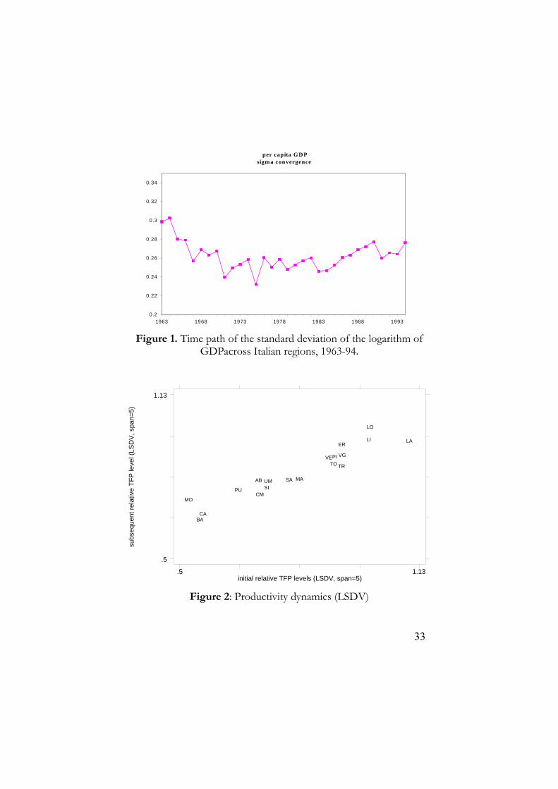
Whatever the reason, the pre- and post-1970 pattern is strongly confirmed by the pattern of σ-convergence for the Italian regions as shown in Figure 1.

As for the distance between top and the bottom regions, during the 1960s per capita income in the richest region, Valle d’Aosta, was 42% (and in Lombardia 38%) wealthier than in the average Italian region. On the other side, the poorest regions, Calabria and Basilicata, had a 38% disadvantage with respect to the Italian average. This is a very large regional gap by any European standard. This gap has diminished during the last three decades but, again, the decrease was neither persistent nor uniform, and came to a halt in the mid-1970s.

3. A Panel Data approach to estimate TFP convergence

Our aim is to test for the presence of TFP heterogeneity and convergence in cross-country convergence analysis by using an appropriate fixed-effect panel estimator. As said above, TFP levels are measured by means of two main methodologies, namely the level

14 See Mauro and Podrecca (1994), Di Liberto (1994), Boltho, Carlin and Scaramozzino

(1999), Paci and Pigliaru (1995) among others. 15 See Graziani (1978). 16 Indeed, stops and goes in regional convergence has been detected in several other

countries. See de la Fuente (1997) for Spanish regions and Sala-i-Martin (1996) for examples from other OECD countries.

7

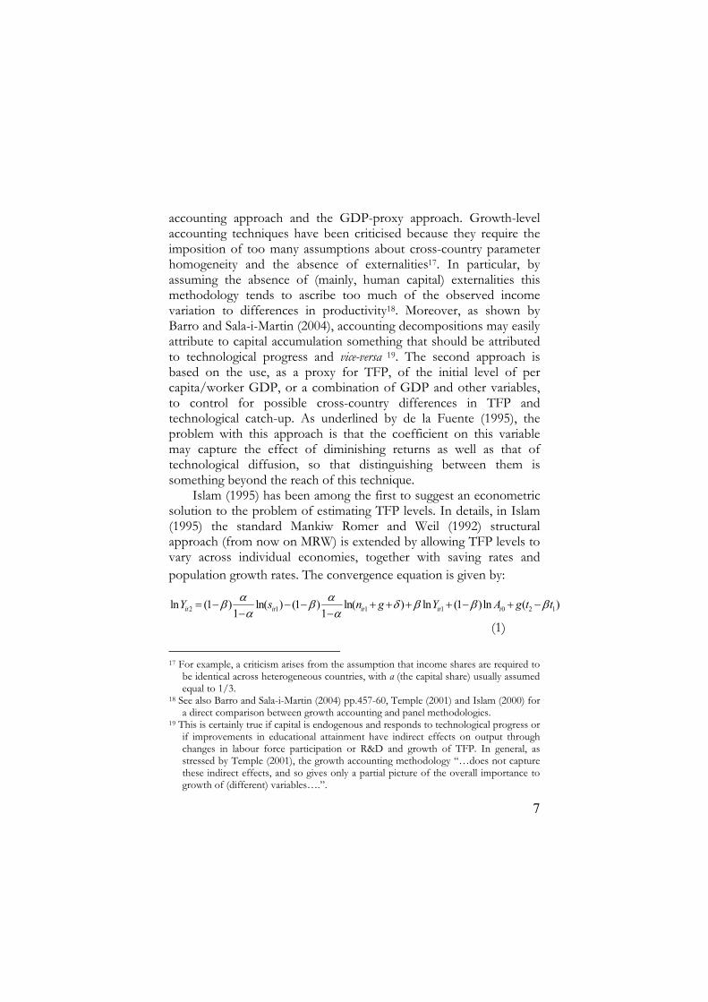
accounting approach and the GDP-proxy approach. Growth-level accounting techniques have been criticised because they require the imposition of too many assumptions about cross-country parameter homogeneity and the absence of externalities17. In particular, by assuming the absence of (mainly, human capital) externalities this methodology tends to ascribe too much of the observed income variation to differences in productivity18. Moreover, as shown by Barro and Sala-i-Martin (2004), accounting decompositions may easily attribute to capital accumulation something that should be attributed to technological progress and vice-versa 19. The second approach is based on the use, as a proxy for TFP, of the initial level of per capita/worker GDP, or a combination of GDP and other variables, to control for possible cross-country differences in TFP and technological catch-up. As underlined by de la Fuente (1995), the problem with this approach is that the coefficient on this variable may capture the effect of diminishing returns as well as that of technological diffusion, so that distinguishing between them is something beyond the reach of this technique.

Islam (1995) has been among the first to suggest an econometric solution to the problem of estimating TFP levels. In details, in Islam (1995) the standard Mankiw Romer and Weil (1992) structural approach (from now on MRW) is extended by allowing TFP levels to vary across individual economies, together with saving rates and population growth rates. The convergence equation is given by:

2 1 1 1 0 2 1ln (1 ) ln( ) (1 ) ln( ) ln (1 )ln ( )1 1it it it it iY s n g Y A g t tα αβ β δ β β β

α α= − − − + + + + − + −

− − (1)

17 For example, a criticism arises from the assumption that income shares are required to

be identical across heterogeneous countries, with α (the capital share) usually assumed equal to 1/3.

18 See also Barro and Sala-i-Martin (2004) pp.457-60, Temple (2001) and Islam (2000) for a direct comparison between growth accounting and panel methodologies.

19 This is certainly true if capital is endogenous and responds to technological progress or if improvements in educational attainment have indirect effects on output through changes in labour force participation or R&D and growth of TFP. In general, as stressed by Temple (2001), the growth accounting methodology “…does not capture these indirect effects, and so gives only a partial picture of the overall importance to growth of (different) variables….”.

8

where

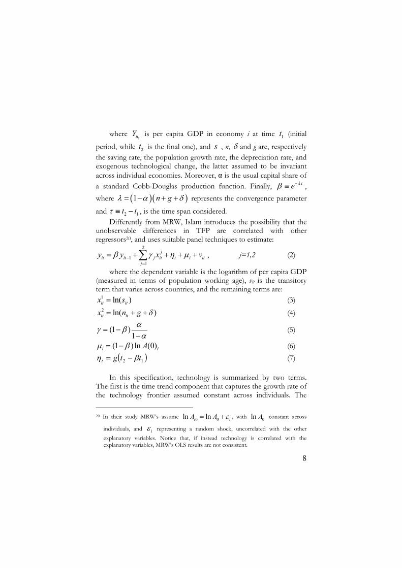
1itY is per capita GDP in economy i at time 1t (initial

period, while 2t is the final one), and s , n, δ and g are, respectively the saving rate, the population growth rate, the depreciation rate, and exogenous technological change, the latter assumed to be invariant across individual economies. Moreover, α is the usual capital share of a standard Cobb-Douglas production function. Finally, e λτβ −≡ , where ( )( )1 n gλ α δ= − + + represents the convergence parameter

and 2 1t tτ ≡ − , is the time span considered. Differently from MRW, Islam introduces the possibility that the

unobservable differences in TFP are correlated with other regressors20, and uses suitable panel techniques to estimate:

2

11

jit it j it t i it

j

y y x vβ γ η µ−=

= + + + +∑ , j=1,2 (2)

where the dependent variable is the logarithm of per capita GDP (measured in terms of population working age), vit is the transitory term that varies across countries, and the remaining terms are:

1 ln( )it itx s= (3) 2 ln( )it itx n g δ= + + (4)

(1 )1αγ βα

= −−

(5)

(1 ) ln (0)i iAµ β= − (6) ( )12 ttgt βη −= (7)

In this specification, technology is summarized by two terms.

The first is the time trend component that captures the growth rate of the technology frontier assumed constant across individuals. The 20 In their study MRW’s assume 0 0ln lni iA A ε= + , with 0ln A constant across

individuals, and iε representing a random shock, uncorrelated with the other explanatory variables. Notice that, if instead technology is correlated with the explanatory variables, MRW’s OLS results are not consistent.

9

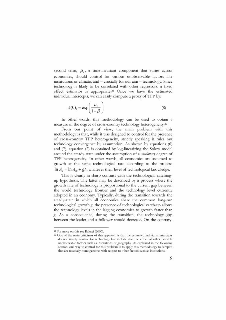
second term, iµ , a time-invariant component that varies across economies, should control for various unobservable factors like institutions or climate, and – crucially for our aim – technology. Since technology is likely to be correlated with other regressors, a fixed effect estimator is appropriate.21 Once we have the estimated individual intercepts, we can easily compute a proxy of TFP by:

(0) exp1

iiA µ

β⎛ ⎞

= ⎜ ⎟−⎝ ⎠ (8)

In other words, this methodology can be used to obtain a measure of the degree of cross-country technology heterogeneity.22

From our point of view, the main problem with this methodology is that, while it was designed to control for the presence of cross-country TFP heterogeneity, strictly speaking it rules out technology convergence by assumption. As shown by equations (6) and (7), equation (2) is obtained by log-linearizing the Solow model around the steady-state under the assumption of a stationary degree of TFP heterogeneity. In other words, all economies are assumed to growth at the same technological rate according to the process

0ln lnit iA A gt= + , whatever their level of technological knowledge. This is clearly in sharp contrast with the technological catching-

up hypothesis. The latter may be described by a process where the growth rate of technology is proportional to the current gap between the world technology frontier and the technology level currently adopted in an economy. Typically, during the transition towards the steady-state in which all economies share the common long-run technological growth g, the presence of technological catch-up allows the technology levels in the lagging economies to growth faster than g. As a consequence, during the transition, the technology gap between the leader and a follower should decrease. On the contrary,

21 For more on this see Baltagi (2003). 22 One of the main criticisms of this approach is that the estimated individual intercepts

do not simply control for technology but include also the effect of other possible unobservable factors such as institutions or geography. As explained in the following section, one way to control for this problem is to apply this methodology to samples that are relatively homogeneous with respect to other factors such as institutions.

10

if no systematic process of technology diffusion is at work, this gap should stay constant over time, since all economies grow at a common rate of technology growth.

How can we use equation (2) to test for the presence/absence of technological convergence? First, notice that, the longer the time dimension of the panel, the higher the risk that differences in TFP levels are not stationary within the sample period, since technological diffusion is more likely to be at work. As a consequence, in the presence of technological convergence equation (2) should be regarded as an approximation of the real process – an approximation that worsens as the length of the period under analysis increases.

Second, and consequently, the presence of technological convergence should be detected by comparing the TFP values obtained by estimating (8) over different periods. This type of comparison should reveal whether the observed pattern of TFP values is consistent either with the catching-up hypothesis or with the alternative hypothesis that the current degree of technology heterogeneity is at its stationary value.

The technique we use follows several, simple steps. First, we estimate equation (2) over different sub-periods, in order to obtain a sequence of estimated values of individual intercepts. Second, the latter values are used to compute the individual values of ln iA .23 Third, we analyse the evolution over time of the distribution of ln iA in order to test for the presence of technological convergence. Indeed, while technology convergence implies a variance of ln iA that decreases over time while approaching its stationary value, the alternative hypothesis implies that the variance of ln iA is at its stationary value, and thus no significant trend in its value should be detected.

23 A similar approach has been previously introduced by Islam (2000)., where the author

compares the distribution of the estimated fixed effects over two points in time. However, in his paper the possibility that technology convergence lies behind the observed changes in the distribution is neither discussed nor tested.

11

4. Comparing the available estimation procedures

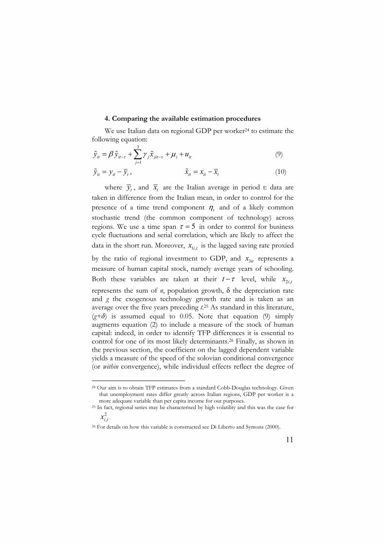
We use Italian data on regional GDP per worker24 to estimate the following equation:

3

1it it j jit i it

j

y y x uτ τβ γ µ− −=

= + + +∑% % % (9)

it it ty y y= −% , it it tx x x= −% (10)

where ty , and tx are the Italian average in period t: data are taken in difference from the Italian mean, in order to control for the presence of a time trend component tη and of a likely common stochastic trend (the common component of technology) across regions. We use a time span 5τ = in order to control for business cycle fluctuations and serial correlation, which are likely to affect the data in the short run. Moreover, 1 ,i tx is the lagged saving rate proxied

by the ratio of regional investment to GDP, and 3itx represents a measure of human capital stock, namely average years of schooling. Both these variables are taken at their t τ− level, while 2 ,i tx represents the sum of n, population growth, δ the depreciation rate and g the exogenous technology growth rate and is taken as an average over the five years preceding t.25 As standard in this literature, (g+δ) is assumed equal to 0.05. Note that equation (9) simply augments equation (2) to include a measure of the stock of human capital: indeed, in order to identify TFP differences it is essential to control for one of its most likely determinants.26 Finally, as shown in the previous section, the coefficient on the lagged dependent variable yields a measure of the speed of the solovian conditional convergence (or within convergence), while individual effects reflect the degree of

24 Our aim is to obtain TFP estimates from a standard Cobb-Douglas technology. Given

that unemployment rates differ greatly across Italian regions, GDP per worker is a more adequate variable than per capita income for our purposes.

25 In fact, regional series may be characterised by high volatility and this was the case for 2,i tx .

26 For details on how this variable is constructed see Di Liberto and Symons (2000).

12

TFP heterogeneity. The first problem we face when we estimate a dynamic panel

data model such as the one represented by equation (9) is which estimator suits our case better. The answer is not simple. It is still true today what Kiviet wrote a few years ago: “As yet, no technique is available that has shown uniform superiority in finite samples over a wide range of relevant situations as far as the true parameter values and the further properties of the DGP are concerned.”27 Indeed, the LSDV estimator, while consistent for large T,28 is characterised by small sample problems and, in particular, it is well known to produce downward biased estimates in small samples. Conversely, the Arellano and Bond (1991) estimator (GMM-AB from now on) is becoming increasingly popular since it has both the advantage of producing consistent estimates in a dynamic panel regression with both (i) endogenous right hand side variables, and (ii) presence of measurement error. Moreover, it is more efficient than other standard IV estimators such as the Anderson-Hsiao estimator. However, it has been recently shown29 that, when T is small, and either the autoregressive parameter is close to one (highly persistent series), or the variance of the individual effect is high relative to the variance of the transient shock, then even the GMM-AB estimator is biased30 and, in particular, downward biased. Note that the presence of a relatively small number of time periods and persistent time series are typical features of macro-growth datasets like ours.

To control for this problem, Kiviet (1995) put forward a more direct approach to the problem of the LSDV finite sample bias by estimating a small sample correction to the LSDV estimator. Monte Carlo analysis31 finds that for small T (such as the one we find in the convergence literature) LSDV estimates corrected for the bias (KIVIET from now on) seem more attractive than GMM. In particular, these Monte Carlo studies explicitly analyse typical macro 27 See Kiviet (1995) pp.72. 28 See Amemyia (1967). 29 See Blundell and Bond (1998) and Bond-Hoeffler-Temple (2001). 30 It may be that the inclusion of additional explanatory variables among regressors and

the inclusion of additional lags of these regressors among instruments will improve the performance of this estimator. See Bond-Hoeffler-Temple (2001).

31 See Kiviet (1995) and Judson and Owen (1996).

13

dynamic panels and find that for 20T ≤ and 50N ≤ , as in our case, the KIVIET and Anderson-Hsiao estimators consistently outperform GMM-AB. Moreover, despite having a higher average bias, KIVIET turns out to be more efficient than Anderson-Hsiao. Overall, these Monte Carlo analyses suggest that a reasonable strategy would be to use the KIVIET estimator for smaller panels ( 10T ≤ ), while Anderson-Hsiao should be preferred for larger panels, as the efficiency of the latter improves with T (Anderson-Hsiao has the additional advantage of being computationally simpler than the former).

Let us now turn to our specific case. Our Italian regional panel includes the period 1963-93 for 19 regions.32 Using the five-year time span implies that we are left with T=7 observations for each of the N=19 regions, corresponding to 1963, 1968, 1973, 1978, 1983, 1988, and 1993. Since, as we noticed above, no technique shows a clear superiority in finite samples, in the following we will use several estimators and will compare their results in order to assess their robustness. In doing this, given the dimension of our panel and the above discussion, the Kiviet-corrected LSDV estimator will be used as our benchmark.33

Since all these estimators perform poorly in small samples, to evaluate how each of them performs in our case we start our empirical analysis by using the whole sample 1963-93. Table 1 shows our results for this case. For each regression we include the estimates obtained and the implied λ̂ , i.e. the speed of solovian convergence parameter.34

Let us start by comparing the results obtained by using the pooling-OLS estimator and the (uncorrected) LSDV estimator. As expected, when we introduce the pooling-OLS estimator (Model 1), the coefficient on the lagged dependent variable is high compared with other individual effects estimators, with a corresponding speed

32 The Italian regions are 20. We have excluded Valle d’Aosta because it represents an

outlier. Nevertheless, results do not change if we include this region. 33 To implement the Kiviet’s small-sample correction we use the STATA routine

proposed by Adam (1998). 34 From te λβ −=

14

of solovian convergence of 3%. Among the regressors, only the coefficients on the lagged dependent variable and on population growth are significant, while both the coefficient on the investment share and on human capital are not significant. These results are robust as they remain stable when other estimation procedure are introduced. When equation (9) is estimated with LSDV (Model 5) we find a lower AR(1) coefficient and a correspondingly higher speed of solovian convergence of 9%.

Let us now extend our comparison to the other available estimators. Both the GMM-AB and the Kiviet correction require us to drop one initial observation.35 Consequently, in order to compare the results of all the different estimators we perform again the regressions discussed in the previous paragraph excluding the first observation. With this reduced sample, the estimated AR(1) OLS parameter (Model 2) is lower than before and equal to 0.80, while the estimated AR(1) LSDV parameter (Model 6) declines to 0.51. The use of the Kiviet correction procedure increases the LSDV parameter from 0.51 to 0.67, with a decline in the corresponding speed of convergence coefficient from 13% to 8%. Note that KIVIET only corrects the bias in the LSDV estimated parameters but does not produce alternative or corrected standard errors. This is why they are not shown among results.

The GMM-AB estimates are shown together with the p-value of the AB-2 statistic and the Sargan test as in Arellano and Bond (1991). The first statistic tests for the presence of serial correlation. In particular, since the final regression equation is in first differences, it tests for second order serial correlation in the error term. The latter must be absent for the assumption of no serial correlation in the model in levels to be accepted. The presence of second-order serial correlation would imply that the estimates are inconsistent. The second statistics tests the validity of overidentifying restrictions. The consistency of this estimation procedure crucially depends on the identifying assumption that lagged values of both income and other explanatory variables are valid instruments in these growth 35 To compute the estimated bias the methodology requires the use of a consistent

estimator, such as Anderson-Hsiao or GMM, and the routine used to calculate KIVIET cannot handle missing observation. See Adam (1998).

15

regressions. The GMM-AB estimator may be performed under very different assumptions on the endogeneity of included regressors. In this study we specify two different hypothesis on the 'x s . First, Model 3 (or model GMM-AB1) in Table 1 assumes that all regressors are predetermined, that is [ ] 0it isE x u ≠ for t s< , and [ ] 0it isE x u = for t s≥ . Second, Model 4 (or model GMM-AB2) assumes instead that all 'x s are strictly exogenous, that is, [ ] 0it isE x u = for all t and s.

The results in Table 1 show that both specifications are valid: the p-values of the AB-2 and Sargan tests say that it is not possible to reject the null hypothesis of absence of second-order autocorrelation and that the over-identifying restrictions are valid. Then, the choice between these two specification is not obvious, even if the increase of the p-value of the Sargan test in GMM-AB1 indicates that treating the included regressors as predetermined makes it more difficult to reject the null and, thus, that Model 3 should be preferred to Model 4.

However, these estimates may be biased. To detect a possible bias in our GMM-AB models we follow the procedure (a sort of rule of thumb) suggested by Bond, Hoeffler and Temple (2001). Given that it is well known that OLS is biased upwards in dynamic panels and LSDV is biased downwards, these authors suggest that a consistent estimate should therefore lie between the two. Since we expect that the true parameter values lie somewhere between ˆ

olsβ

and ˆLSDVβ , in our case we expect its value to be between 0.80 and

0.51. The estimated AR(1) coefficient on GMM-AB2 is higher than that obtained with OLS, where the latter should be characterized by upward bias. Consequently, we exclude GMM-AB2 from the following analysis. Conversely, the estimated AR(1) coefficient on GMM-AB1, 0.696, is very similar to that obtained in KIVIET, 0.669. With a value included between ˆ

olsβ and ˆLSDVβ 36, this estimate does

36 The AR(1) coefficient in GMM-AB1 is lower than that in GMM-AB2 also because

treating included regressors as predetermined instead of strictly exogenous increases the size of the instrument matrix and, while additional instruments increase efficiency

16

not suggest any obvious presence of bias. Thus, to sum up, in this section we have seen that previous

Monte Carlo analysis suggest KIVIET as the best estimation procedure to estimate model (9) with samples with similar characteristics as ours. Nevertheless, since LSDV and GMM-AB are both employed estimators in this literature, in the following section we will use LSDV, KIVIET and GMM-AB1 to compute our regional TFP levels and compare the results obtained.

5. Testing for TFP heterogeneity With these estimates in hand we now move on to compute our

regional TFP measures. In our LSDV estimates the regional dummy coefficients, ˆ iµ , are almost invariably statistically significant. As for the GMM-AB (1 and 2) estimator, note that the latter controls for fixed effects by transforming data in first difference and, thus, the individual effects are not directly estimated. Following Caselli, Esquivel and Lefort (1996), we obtain estimates of iµ by:

( )2

1 1 11

ˆ ˆˆ ˆ ˆi it it it j jit itj

u y by x hµ γ ξ− − −=

+ = − − −∑ %% % % (11)

( )1ˆ ˆ ˆi i ituTµ µ= +∑ (12)

The same procedure has been used to obtain ˆ iµ and, through

equation (8) ( )ˆ 0i

A , using KIVIET. In all cases, the TFP estimates

are then used to compute the ratio ( ) ( )ˆ ˆ0 0i Lom

A A , with ( )ˆ 0Lom

A being the estimated TFP value for Lombardia, currently the richest, most industrialised and arguably the most technologically advanced Italian region.

Table 2a includes the estimates of the relative (to Lombardia) levels of regional TFP obtained by applying each different estimator. Moreover, to make the interpretation of results easier, Table 2b shows the ranking that each region obtain with the different

of the GMM procedure, they may also increase the downward bias in a small panel. See also Ayiar and Feyrer (2002).

17

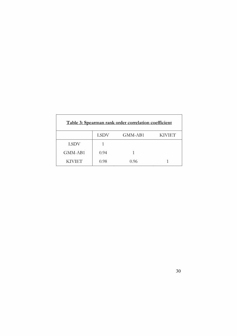
methodologies. Overall, these results suggest that different econometric

methodologies produce similar TFP estimates. This conclusion is confirmed by the analysis of the Spearman rank order coefficient (see Table 3).

As expected, the estimates of the regional relative TFP levels obtained by LSDV and KIVIET are very similar, with a correlation coefficient equal to 0.98. Eight regions out of nineteen hold the same ranking, three regions (Abruzzo, Liguria and Sardegna) change their rank by two positions, while for the remaining regions the rank changes by only one position. A lower but still very high ranking correspondence if found between the LSDV, KIVIET and GMM-AB1 estimates.37

To sum up, the close correspondence found in this section among the TFP estimates obtained with different estimation procedures support the conclusion that our results can be confortably regarded as robust.

More generally, the overall picture emerging from our estimates is an interesting one. In particular, it strongly confirms that TFP differences can be significantly large even across regions, and that an important part of the Italian economic divide seems to be due to such differences. For instance, in 1968 the GDP per worker in Basilicata (the poorest region) was 53% of Lombardia value; in our estimates, the corresponding relative TFP value is even higher (an average of 67,7%: see Table 2a). Moreover, we find confirmation that the northern and richer regions are also the most technologically advanced areas in the country, and that at the bottom end are the southern, less developed areas.

The pattern and the magnitude of TFP heterogeneity as measured by our estimates suggest that a potential for technological catch-up does exist for the lagging regions. In turn, this implies that any analysis of aggregate convergence across Italian regions should

37 For GMM-AB2 the Spearman rank correlation coefficient was lower, ranging from

0.94 (with GMM-AB1) and 0.92 (with LSDV). We have also checked the rank correlation between the initial level of income and the different TFP measures obtained. In this case, the Spearman rank correlation coefficient is 0,87 (with LSDV), 0,82 (with KIVIET), and 0,76 (with GMM-AB1).

18

take this potential source of convergence into account. This is what we will do in the next section.

6. Detecting technological convergence: Empirical results

In the previous section we have shown that a high degree of TFP heterogeneity does exist across the Italian regions. In this section we investigate whether this degree of hereogeneity is either stationary or is the source of a process of TFP convergence. As suggested by Islam (2003) and Pigliaru (2003), to test for the presence of TFP convergence we need to generate TFP-level indices for several consecutive time periods, so that the TFP dynamics can be directly analysed. The indices produced by panel methods may be used to this end as “…they contain ordinal as well as cardinal information, which can both be helpful in answering questions regarding TFP-convergence”.38 The main difficulty with this procedure is that, in order to generate different TFP-level indices for consecutive time periods we need to further reduce the time dimension of the estimated samples, thus worsening the problems associated with small sample bias discussed above. Note that using a time span equal to 5 implies that we are left with T=7 observations, which in turn implies T=6 in LSDV because of the presence of the lagged dependent variable among regressors, and T=5 with Kiviet since it uses the Anderson-Hsiao estimates to calculate the bias.39

With such a dataset it is possible to obtain two sub-samples and to apply LSDV to estimate regional TFP levels, but the implementation of the KIVIET correction procedure to these short sub-samples becomes infeasible. A possible alternative is to gain degrees of freedom by using a shorter time span. For example, a time span equal to three ( 3τ = ) yields T=11 (i.e., T=10 with LSDV and T=9 with KIVIET). Clearly, using a shorter time span has the obvious disadvantage that it increases the problems related to short

38 See Islam (2003), pp.349. 39 In this case data are taken in first difference and levels of the dependent variable

(lagged twice and further) are introduced as instruments. For more details see Baltagi (2003).

19

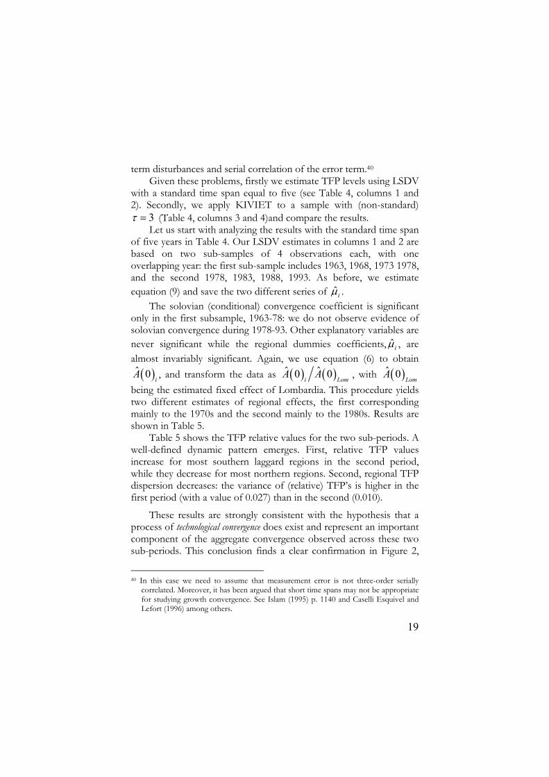
term disturbances and serial correlation of the error term.40 Given these problems, firstly we estimate TFP levels using LSDV

with a standard time span equal to five (see Table 4, columns 1 and 2). Secondly, we apply KIVIET to a sample with (non-standard)

3τ = (Table 4, columns 3 and 4)and compare the results. Let us start with analyzing the results with the standard time span

of five years in Table 4. Our LSDV estimates in columns 1 and 2 are based on two sub-samples of 4 observations each, with one overlapping year: the first sub-sample includes 1963, 1968, 1973 1978, and the second 1978, 1983, 1988, 1993. As before, we estimate equation (9) and save the two different series of ˆ iµ .

The solovian (conditional) convergence coefficient is significant only in the first subsample, 1963-78: we do not observe evidence of solovian convergence during 1978-93. Other explanatory variables are never significant while the regional dummies coefficients, ˆ iµ , are almost invariably significant. Again, we use equation (6) to obtain ( )ˆ 0

iA , and transform the data as ( ) ( )ˆ ˆ0 0

i LomA A , with ( )ˆ 0

LomA

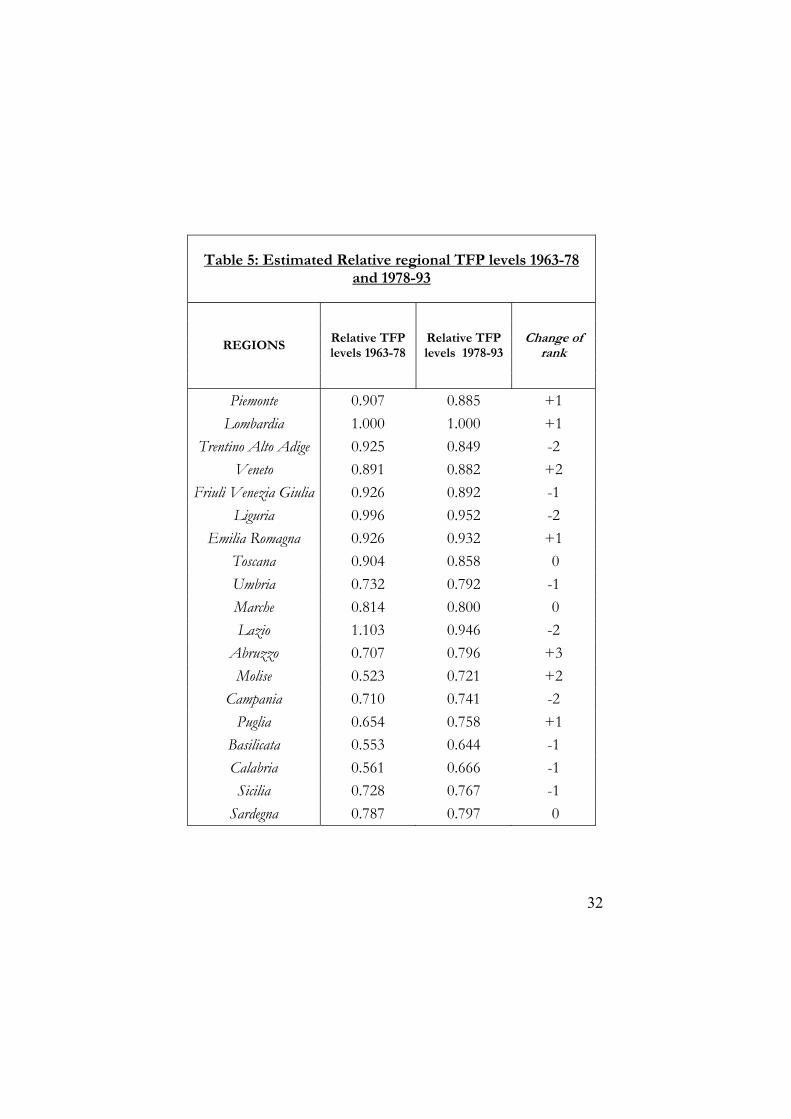
being the estimated fixed effect of Lombardia. This procedure yields two different estimates of regional effects, the first corresponding mainly to the 1970s and the second mainly to the 1980s. Results are shown in Table 5.

Table 5 shows the TFP relative values for the two sub-periods. A well-defined dynamic pattern emerges. First, relative TFP values increase for most southern laggard regions in the second period, while they decrease for most northern regions. Second, regional TFP dispersion decreases: the variance of (relative) TFP’s is higher in the first period (with a value of 0.027) than in the second (0.010).

These results are strongly consistent with the hypothesis that a process of technological convergence does exist and represent an important component of the aggregate convergence observed across these two sub-periods. This conclusion finds a clear confirmation in Figure 2,

40 In this case we need to assume that measurement error is not three-order serially

correlated. Moreover, it has been argued that short time spans may not be appropriate for studying growth convergence. See Islam (1995) p. 1140 and Caselli Esquivel and Lefort (1996) among others.

20

where the relationship existing between the TFP estimated for the 1963-79 interval and the subsequent one is shown.

The dotted 45 degree line shows the locus where the relative TFP level in each region would be unchanged between the two periods. Most southern regions are clearly above the 45 degree line41 as they performed consistently better in term of relative TFP growth, while six (northern) regions are below the 45 degree line. This pattern is consistent with the hypothesis of TFP convergence.

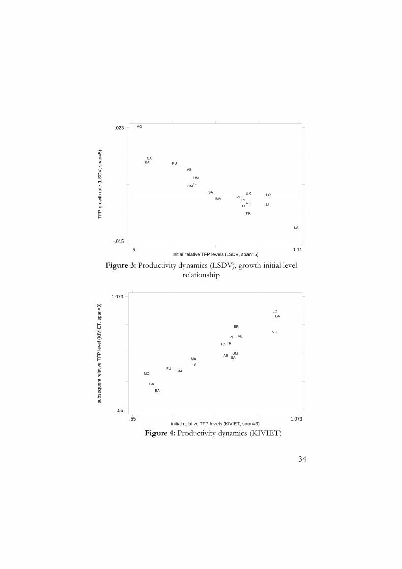
The same data may be rearranged to analyse this result in terms of a typical growth-initial level convergence relationship. In Figure 3 the Y-axis represents the rate of growth of relative TFP, while the X-axis represents the initial relative TFP level. Convergence implies a negative correlation between the initial level of TFP and its subsequent growth rate. This is exactly what our data reveal. Nevertheless, in spite of this clear convergence pattern the distance between northern and southern regions in terms of relative TFP was still significant in the second sub-period, as shown by Table 5.

Let us now go back to Table 4, columns 3 and 4, in order to assess the robustness of our LSDV result by applying the Kiviet-corrected LSDV estimator. When we use the latter, the two sub-samples each include 5 observations, with one overlapping year. The first sub-sample includes 1969, 1972, 1975 1978, 1981, while the second 1981, 1984, 1987, 1990, 1993.42

Models 3 and 4 in Table 4 suggest that, in contrast with LSDV, the solovian (conditional) convergence coefficient is significant in both sub-periods. In the first subsample analysed, the other variables included are never significant, while in the second both ln( )s and ln( )n gδ+ + are negative and significant. Human capital is never significant.

With respect to the TFP estimates, our previous result based on the LSDV estimator does not change significantly. Again, the estimated variance of relative TFP’s is higher in the first period (with 41 These are Molise, Basilicata, Calabria, Puglia, Abruzzo, Umbria Sicilia and Campania. 42 Note that there is not a perfect correspondence between the samples used in LSDV

and KIVIET and, thus, the evidence obtained in the two cases is not perfectly comparable.

21

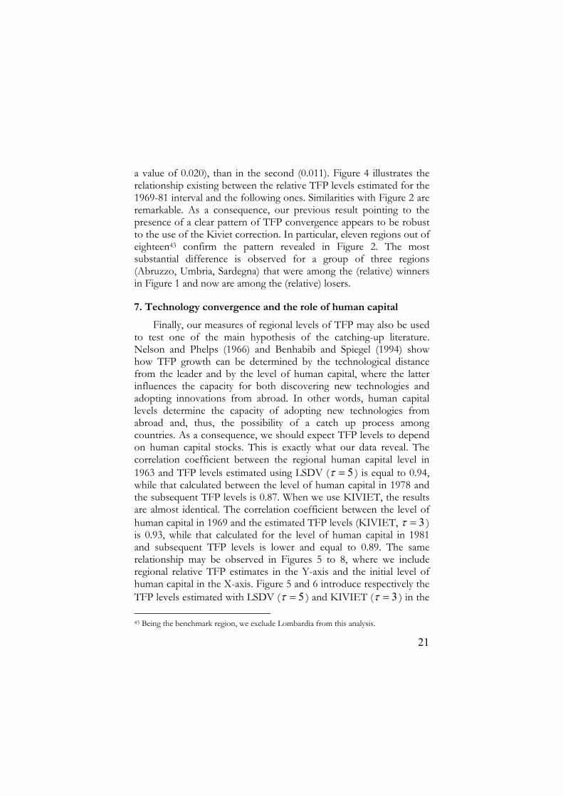
a value of 0.020), than in the second (0.011). Figure 4 illustrates the relationship existing between the relative TFP levels estimated for the 1969-81 interval and the following ones. Similarities with Figure 2 are remarkable. As a consequence, our previous result pointing to the presence of a clear pattern of TFP convergence appears to be robust to the use of the Kiviet correction. In particular, eleven regions out of eighteen43 confirm the pattern revealed in Figure 2. The most substantial difference is observed for a group of three regions (Abruzzo, Umbria, Sardegna) that were among the (relative) winners in Figure 1 and now are among the (relative) losers.

7. Technology convergence and the role of human capital

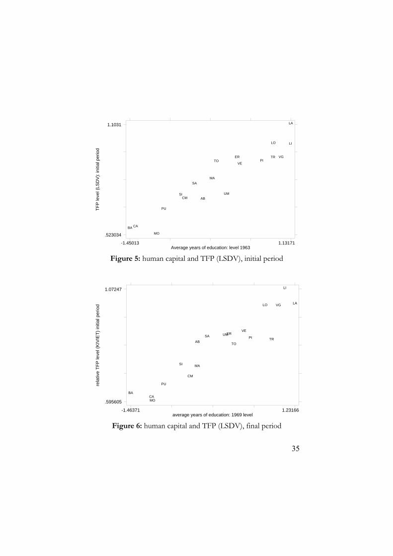
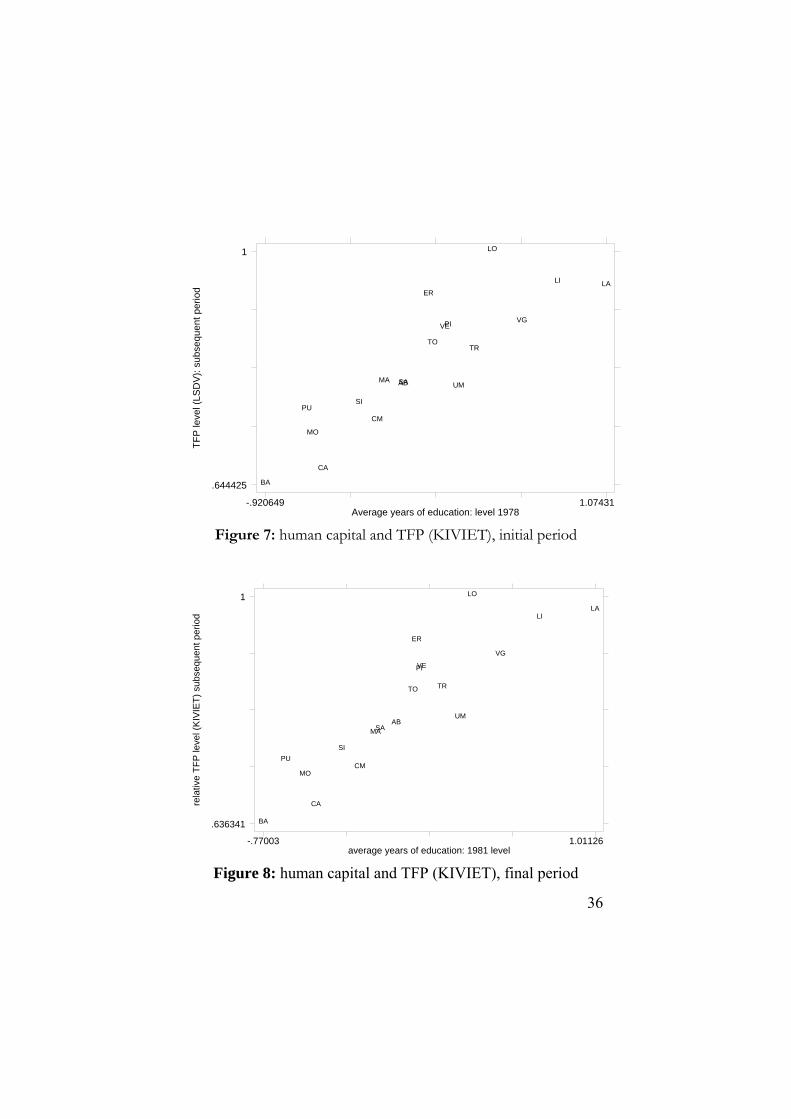
Finally, our measures of regional levels of TFP may also be used to test one of the main hypothesis of the catching-up literature. Nelson and Phelps (1966) and Benhabib and Spiegel (1994) show how TFP growth can be determined by the technological distance from the leader and by the level of human capital, where the latter influences the capacity for both discovering new technologies and adopting innovations from abroad. In other words, human capital levels determine the capacity of adopting new technologies from abroad and, thus, the possibility of a catch up process among countries. As a consequence, we should expect TFP levels to depend on human capital stocks. This is exactly what our data reveal. The correlation coefficient between the regional human capital level in 1963 and TFP levels estimated using LSDV ( 5τ = ) is equal to 0.94, while that calculated between the level of human capital in 1978 and the subsequent TFP levels is 0.87. When we use KIVIET, the results are almost identical. The correlation coefficient between the level of human capital in 1969 and the estimated TFP levels (KIVIET, 3τ = ) is 0.93, while that calculated for the level of human capital in 1981 and subsequent TFP levels is lower and equal to 0.89. The same relationship may be observed in Figures 5 to 8, where we include regional relative TFP estimates in the Y-axis and the initial level of human capital in the X-axis. Figure 5 and 6 introduce respectively the TFP levels estimated with LSDV ( 5τ = ) and KIVIET ( 3τ = ) in the 43 Being the benchmark region, we exclude Lombardia from this analysis.

22

first sub-period of the analysis, while Figure 7 and 8 introduce the same analysis for the second sub-period. In general, this evidence, together with the absence of significance of the human capital variable in our regressions, corroborate the hypothesis of a relationship between human capital and TFP as described by the Nelson and Phelps approach.

8. Conclusion The aim of this paper was to assess the existence of technology

convergence across the Italian regions between 1963 and 1993. Different methodologies have been proposed to measure TFP heterogeneity across countries, but only a few of them try to capture the presence of technology convergence as a separate component from the standard solovian (capital-deepening) source of convergence. To distinguish between these two component of convergence, we have proposed and applied a fixed-effect panel methodology.

Our results show, first of all, the presence of a TFP heterogeneity across Italian regions. This result is robust to the use of different estimation procedure such as simple LSDV, Kiviet-corrected LSDV, and GMM à la Arellano and Bond (1991). Second, we find strong support to the hypothesis that a significant process of TFP convergence has been a key factor in the observed aggregate regional convergence that took place in Italy up to the mid-seventies. To the best of our knowledge, this is the first time that evidence on TFP convergence across Italian regions has been produced in a context in which the traditional Solovian-type of convergence is simultaneously taken into account.

Moreover, our results show that a period of significant convergence in TFP has not generated a significant, persistent decrease in the degree of cross-region inequality in per capita income. The solution to this puzzle may be a simple one. Our evidence shows that technology convergence took place between the two sub-periods of our analysis (1963-78 and 1978-93), while nothing can be inferred on what has happened, in terms of technology diffusion, within the second sub-period. So, one possibility is that the halt of aggregate convergence in this sub-period is due to a halt of technology

23

diffusion. More data and research are needed to test this additional hypothesis.

Finally, our human capital measures has been found to be highly positively correlated with TFP levels. This result confirms one of the hypothesis of the Nelson and Phelps approach, namely that human capital is the main determinant of technological catch-up. This latter result suggests an explanation for the existence of persistent differences in regional GDP per worker: this might be due to the fact that the backward regions never caught-up with the the northern and richest ones in terms of their human capital endowments.

24

References

Adam, C. S. (1998), “Implementing Small-Sample Bias Corrections in Dynamic Panel Data Estimators Using Stata.” Mimeo, University of Oxford.

Aiello and Scoppa (2000), Uneven Regional Development in Italy: Explaining Differences in Productivity Levels, Giornale Degli Economisti e Annali di Economia, 59, 270-98

Aiyar and Feyrer (2002), “A contribution to the empirics of TFP”, mimeo.

Amemiya, T. (1967), “A Note on the Estimation of Balestra-Nerlove Models.” Institute for Mathematical Studies in Social Sciences Technical Report No. 4. Stanford University, Stanford.

Arellano M., and Bond S. (1991), “Some Tests of Specification for Panel Data: Monte Carlo Evidence and an Application to Employment Equations”, Review of Economic Studies 58, 277-97

Baltagi, B. H. 2003. Econometric Analysis of Panel Data. Chichester: John Wiley and Sons.

Barro R. and Sala-i-Martin X. (2004), Economic growth, New York: McGraw-Hill.

Barro, R.J., and Sala-i-Martin, X. (1991), “Convergence Across States and Regions.” Brookings Paper of Economic Activity 0, 107-182.

Baier S. L., Dwyer G. P. and Tamura R. (2002) “How Important are Capital and Total Factor Productivity for Economic Growth?”, Working Paper, Federal Reserve Bank of Atlanta.

Benhabib, J., and Spiegel, M.M. (1994), “The role of human capital in economic development. Evidence from aggregate cross-country data.” Journal of Monetary Economics 34, 143-173.

Bernard A.B. and Jones C.I. (1996), Technology and convergence, Economic Journal, 106, 1037-44.

Boldrin and Canova (2001), Inequality and convergence: reconsidering European regional policies, Economic Policy, n. 32, 205-245

Boltho A., Carlin W. And Scaramozzino P. (1999), Will East Germany become a new Mezzogiorno?, in: J. Adams and F. Pigliaru, editors, Economic Growth and Change. National and Regional Patterns of Convergence and Divergence, Cheltenham: Edward Elgar.

Blundell R. and Bond S. (1998), “Initial Conditions and Moment Restrictions in Dynamic Panel Data Models.” Journal of Econometrics, 87, 115-143.

Bond, S., Hoeffler , A. and Temple, J. (2001), “GMM Estimation of Empirical

25

Growth Models.” Mimeo.

Caselli, F., Esquivel, G., and Lefort, F. (1996), “Reopening the Convergence Debate: a New Look at Cross Country Growth Empirics.” Journal of Economic Growth 1, 363-89.

de la Fuente A. (1997), The empirics of growth and convergence, Journal of Economic Dynamics and Control, 21, 23-77

de la Fuente A. (2002), On the source of convergence: a closer look at the Spanish regions, European Economic Review, 46, 569-599.

Di Liberto A. (1994), “Convergence Across Italian regions.” Nota di Lavoro Fondazione ENI Enrico Mattei No. 68/94. Milano.

Di Liberto (2001) "Stock di Capitale Umano e Crescita delle Regioni Italiane: un Approccio Panel", Politica Economica, 17: 159-184.

Dowrick S. and Nguyen D. (1989), OECD comparative economic growth 1950-85: catch-up and convergence, American Economic Review, 79, 1010-30.

Dowrick and Rogers M. (2002), Classical and technological convergence: beyond the Solow-Swan growth model, Oxford Economic Papers, 54, 369-385.

Easterly W. and Levine R. (2001), . It's Not Factor Accumulation: Stylized Facts and Growth Models, World Bank Economic Review, 15, 177-219.

Fagerberg J. and Verspagen B. (1996), Heading for divergence. Regional growth in Europe riconsidered, Journal of Common Market Studies, 34, 431-48.

Graziani A. (1978), “The Mezzogiorno in the Italian Economy.” Cambridge Journal of Economics 2, 355-72.

Judson, R. and Owen, A. (1996), “Estimating DPD models: a Practical Guide for Macroeconomists.” Federal Reserve Board of Governors mimeo.

Hall R.E. and Jones C.I. (1999), Why do some countries produce so much more output per worker than others?, Quartely Journal of Economics, 114, 83-116.

Islam N. (1995), Growth empirics: a panel data approach, Quarterly Journal of Economics, 110, 1127-1170.

Islam N. (2000), Productivity dynamics in a large sample of countries: a panel study, Emory University, mimeo.

Islam, N. (2003), “What Have we Learnt from the Convergence Debate?.” Journal of Economic Survey 17, 309-62.

Kiviet, J. (1995), “On Bias, Inconsistency, and Efficiency of Various

26

Estimators in Dynamicc Panel Data Models.” Journal of Econometrics, 68, pp. 53-78.

Klenow P.J. and Rodriguez-Clare A. (1997), Economic Growth: A Review Essay, Journal of Monetary Economics, 40, 597-617.

Lucas R. E. (2000), Some macroeconomics for the 21st century, Journal of Economic Perspectives, 14, 159-168.

Mankiw N.G., Romer D. and Weil D. (1992), A contribution to the empirics of economic growth, Quarterly Journal of Economics, 107, 407-37.

Marrocu E., Paci R. and Pala R. (2001), Estimation of Total Factor Productivity for Regions and Sectors in Italy: A Panel Cointegration Approach, Rivista Internazionale di Scienze Economiche e Commerciali, 48, 533-558.

Mauro, L., and Podrecca, E. (1994), “The case of Italian Regions: Convergence or Dualism?” Economic Notes 24, 447-472.

Nelson, R. R., and Phelps, E. S. (1966), “Investments in Humans, Technological Diffusion, and Economic Growth.” American Economic Review 56, 69-75.

Paci R. and Pigliaru F. (1995), Differenziali di crescita nelle regioni italiane: un'analisi cross-section, Rivista di Politica Economica, LXXXV, pp. 3-34.

Paci R. and Pigliaru F. (2002), Technological diffusion, spatial spillovers and regional convergence in Europe, in: J.R. Cuadrado-Roura and M. Parellada (eds), Regional convergence in the European Union, Berlin: Springer, 273-292.

Parente S.L. and Prescott E.C. (2000), Barriers to the Riches, Boston: MIT Press.

Pigliaru F. (2003), Detecting technological catch-up in economic convergence, Metroeconomica, 54, 161-178

Sala-i-Martin X. (1996), “The Classical Approach to Convergence Analysis.” The Economic Journal 106, 1019-1036.

Temple J. (2001), “Growth Effects of Education and Social Capital in the OECD Countries.” Mimeo, University of Bristol.

Young, A. (1994), “Lessons from the East Asian NIC’s. A Contrarian View.” European Economic Reviw 38, 964-73.

Young, A. (1995), “Confronting the Statistical Realities of the East Asian Growth Experience.” Quarterly Journal of Economics 110, 641-80.

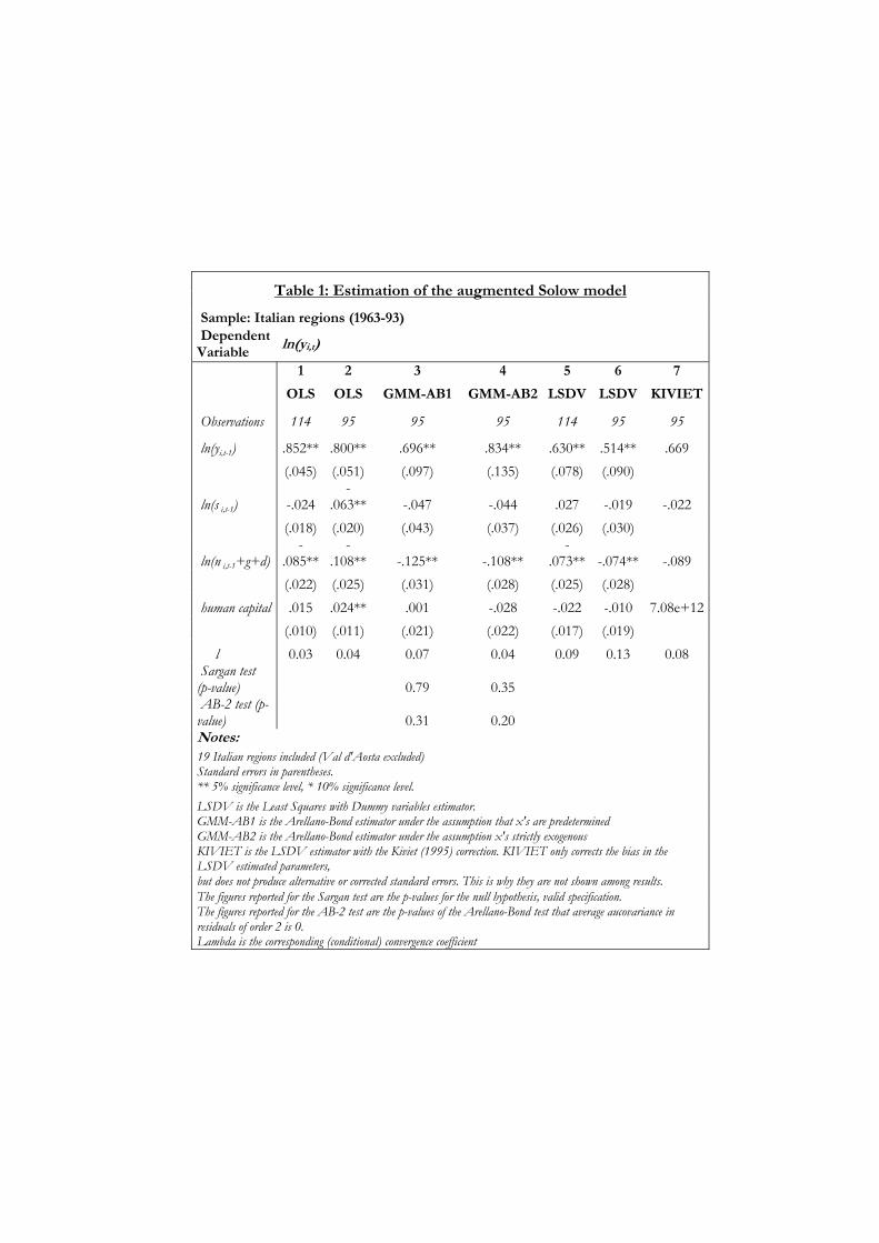
Table 1: Estimation of the augmented Solow model

Sample: Italian regions (1963-93) Dependent Variable

ln(yi,t) 1 2 3 4 5 6 7

OLS OLS GMM-AB1 GMM-AB2 LSDV LSDV KIVIET

Observations 114 95 95 95 114 95 95

ln(yi,t-1) .852** .800** .696** .834** .630** .514** .669 (.045) (.051) (.097) (.135) (.078) (.090)

ln(s i,t-1) -.024 -

.063** -.047 -.044 .027 -.019 -.022 (.018) (.020) (.043) (.037) (.026) (.030)

ln(n i,t-1+g+d)-

.085** -

.108** -.125** -.108** -

.073** -.074** -.089 (.022) (.025) (.031) (.028) (.025) (.028) human capital .015 .024** .001 -.028 -.022 -.010 7.08e+12 (.010) (.011) (.021) (.022) (.017) (.019) l 0.03 0.04 0.07 0.04 0.09 0.13 0.08 Sargan test (p-value) 0.79 0.35 AB-2 test (p-value) 0.31 0.20 Notes: 19 Italian regions included (Val d'Aosta excluded) Standard errors in parentheses. ** 5% significance level, * 10% significance level. LSDV is the Least Squares with Dummy variables estimator. GMM-AB1 is the Arellano-Bond estimator under the assumption that x's are predetermined GMM-AB2 is the Arellano-Bond estimator under the assumption x's strictly exogenous KIVIET is the LSDV estimator with the Kiviet (1995) correction. KIVIET only corrects the bias in the LSDV estimated parameters, but does not produce alternative or corrected standard errors. This is why they are not shown among results. The figures reported for the Sargan test are the p-values for the null hypothesis, valid specification. The figures reported for the AB-2 test are the p-values of the Arellano-Bond test that average aucovariance in residuals of order 2 is 0. Lambda is the corresponding (conditional) convergence coefficient

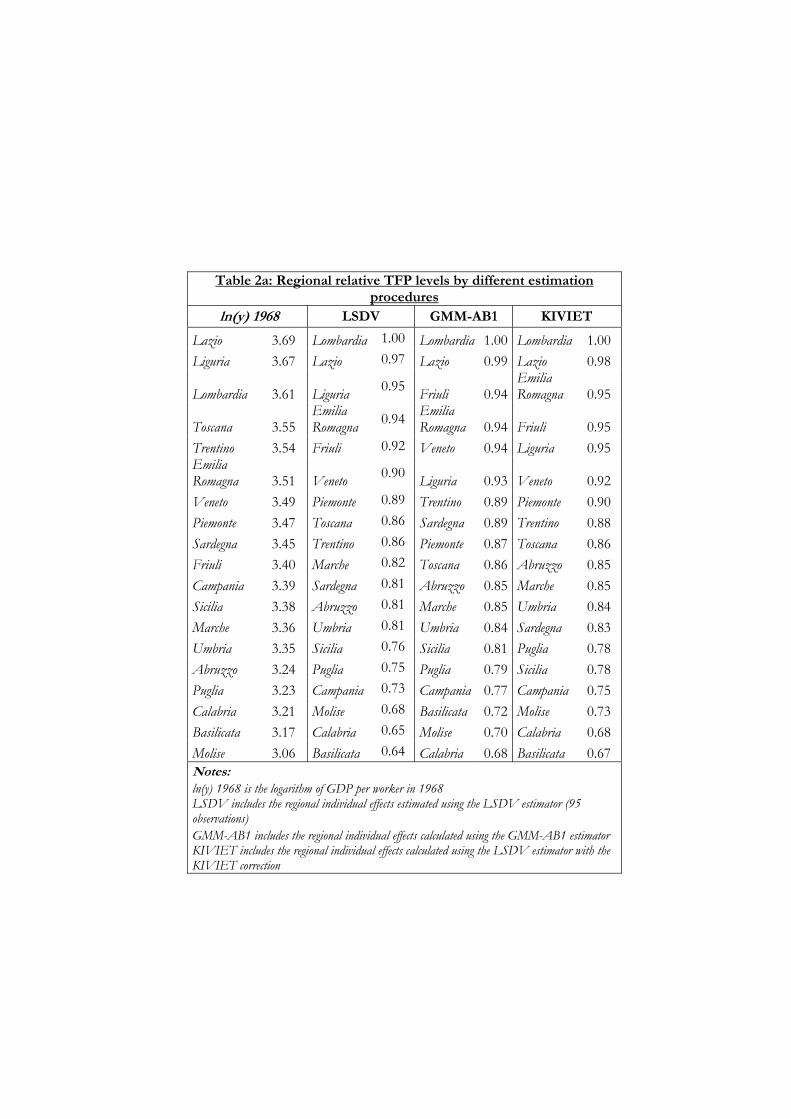
Table 2a: Regional relative TFP levels by different estimation procedures

ln(y) 1968 LSDV GMM-AB1 KIVIET

Lazio 3.69 Lombardia 1.00 Lombardia 1.00 Lombardia 1.00 Liguria 3.67 Lazio 0.97 Lazio 0.99 Lazio 0.98

Lombardia 3.61 Liguria 0.95 Friuli 0.94Emilia Romagna 0.95

Toscana 3.55 Emilia Romagna 0.94 Emilia

Romagna 0.94 Friuli 0.95 Trentino 3.54 Friuli 0.92 Veneto 0.94 Liguria 0.95 Emilia Romagna 3.51 Veneto 0.90 Liguria 0.93 Veneto 0.92 Veneto 3.49 Piemonte 0.89 Trentino 0.89 Piemonte 0.90 Piemonte 3.47 Toscana 0.86 Sardegna 0.89 Trentino 0.88 Sardegna 3.45 Trentino 0.86 Piemonte 0.87 Toscana 0.86 Friuli 3.40 Marche 0.82 Toscana 0.86 Abruzzo 0.85 Campania 3.39 Sardegna 0.81 Abruzzo 0.85 Marche 0.85 Sicilia 3.38 Abruzzo 0.81 Marche 0.85 Umbria 0.84 Marche 3.36 Umbria 0.81 Umbria 0.84 Sardegna 0.83 Umbria 3.35 Sicilia 0.76 Sicilia 0.81 Puglia 0.78 Abruzzo 3.24 Puglia 0.75 Puglia 0.79 Sicilia 0.78 Puglia 3.23 Campania 0.73 Campania 0.77 Campania 0.75 Calabria 3.21 Molise 0.68 Basilicata 0.72 Molise 0.73 Basilicata 3.17 Calabria 0.65 Molise 0.70 Calabria 0.68 Molise 3.06 Basilicata 0.64 Calabria 0.68 Basilicata 0.67 Notes: ln(y) 1968 is the logarithm of GDP per worker in 1968 LSDV includes the regional individual effects estimated using the LSDV estimator (95 observations) GMM-AB1 includes the regional individual effects calculated using the GMM-AB1 estimator KIVIET includes the regional individual effects calculated using the LSDV estimator with the KIVIET correction

29

Table 2b: Regional TFP ranks by different estimation procedures

Regions Rank with

LSDV Rank with GMM-AB1

Rank with GMM-AB2

Rank with KIVIET

Abruzzo 12 11 9 10

Basilicata 19 17 18 19

Calabria 18 19 19 18

Campania 16 16 15 16

Emilia Romagna 4 4 6 3

Friuli 5 3 1 4

Lazio 2 2 2 2

Liguria 3 6 4 5

Lombardia 1 1 3 1

Marche 10 12 12 11

Molise 17 18 17 17

Piemonte 7 9 10 7

Puglia 15 15 16 14

Sardegna 11 8 11 13

Sicilia 14 14 14 15

Toscana 8 10 13 9

Trentino 9 7 7 8

Umbria 13 13 8 12

Veneto 6 5 5 6 Notes: LSDV includes the rank of regional individual effects estimated using the LSDV estimator (95 observations)

GMM-AB1 includes the rank of regional individual effects calculated using the GMM-AB1 estimator KIVIET includes the rank of regional individual effects calculated using the LSDV estimator with the KIVIET correction

30

Table 3: Spearman rank order correlation coefficient

LSDV GMM-AB1 KIVIET

LSDV 1

GMM-AB1 0.94 1

KIVIET 0.98 0.96 1

31

Table 4: Estimation of the augmented Solow model (two subsamples)

Sample: Italian regions 1963-978 and 1978-93 Dependent Variable ln(yi,t) 1 2 3 4

time span=5 time span=5 time span=3 time span=3 1963-1978 1978-1993 1963-1981 1981-1993

LSDV LSDV KIVIET KIVIET

Observations 57 57 95 95

ln(yi,t-1) .480** .015 .760** .386** (.141) (.124) ln(s i,t-1) .055 -.051 -.068 -.061** (.049) (.036) ln(n i,t-

1+g+d) -.061 -.069** -.047 -.062** (.052) (.027) human capital -.051 .006 -.30 .013 (.052) (.044) l 0.15 0.84 0.09 0.32 Notes: 19 Italian regions included (Val d'Aosta excluded) Standard errors in parentheses. ** 5% significance level, * 10% significance level LSDV is the Least Squares with Dummy variables estimator. KIVIET is the LSDV estimator with the Kiviet (1995) correction and only corrects the bias in the estimated parameters. It does not produce alternative or corrected standard errors. This is why they are not shown among results. Lambda is the corresponding (conditional) convergence coefficient

32

Table 5: Estimated Relative regional TFP levels 1963-78 and 1978-93

REGIONS Relative TFP levels 1963-78

Relative TFP levels 1978-93

Change of rank

Piemonte 0.907 0.885 +1 Lombardia 1.000 1.000 +1

Trentino Alto Adige 0.925 0.849 -2 Veneto 0.891 0.882 +2

Friuli Venezia Giulia 0.926 0.892 -1 Liguria 0.996 0.952 -2

Emilia Romagna 0.926 0.932 +1 Toscana 0.904 0.858 0 Umbria 0.732 0.792 -1 Marche 0.814 0.800 0 Lazio 1.103 0.946 -2

Abruzzo 0.707 0.796 +3 Molise 0.523 0.721 +2

Campania 0.710 0.741 -2 Puglia 0.654 0.758 +1

Basilicata 0.553 0.644 -1 Calabria 0.561 0.666 -1 Sicilia 0.728 0.767 -1

Sardegna 0.787 0.797 0

33

Figure 1. Time path of the standard deviation of the logarithm of GDPacross Italian regions, 1963-94.

Figure 1

Figure 2: Productivity dynamics (LSDV)

Figure 2: Productivity dynamics (LSDV)

subs

eque

nt re

lativ

e TF

P le

vel (

LSD

V, s

pan=

5)

initial relative TFP levels (LSDV, span=5).5 1.13

.5

1.13

PI

LO

TR

VE VG

LIER

TO

UM MA

LA

AB

MOCM

PU

BACA

SISA

per capita GD Psigm a convergence

0.2

0.22

0.24

0.26

0.28

0.3

0.32

0.34

1963 1968 1973 1978 1983 1988 1993

34

TFP

gro

wth

rate

(LS

DV

, spa

n=5)

initial relative TFP levels (LSDV, span=5).5 1.11

-.015

.023

PILO

TR

VE

VG LI

ER

TO

UM

MA

LA

AB

MO

CM

PUBACA

SI

SA

Figure 3: Productivity dynamics (LSDV), growth-initial level

relationship

Figure 4: Productivity dynamics (KIVIET)

Figure 4: Productivity dynamics (KIVIET)

subs

eque

nt re

lativ

e TF

P le

vel (

KIV

IET,

spa

n=3)

initial relative TFP levels (KIVIET, span=3).55 1.073

.55

1.073

PI

LO

TR

VEVG

LI

ER

TO

UMMA

LA

AB

MOCM

PU

BA

CA

SI

SA

35

TFP

leve

l (LS

DV

): in

itial

per

iod

Average years of education: level 1963-1.45013 1.13171

.523034

1.1031

PI

LO

TR

VE

VG

LI

ERTO

UM

MA

LA

AB

MO

CM

PU

BA CA

SI

SA

Figure 5: human capital and TFP (LSDV), initial period

rela

tive

TFP

leve

l (K

IVIE

T) in

itial

per

iod

average years of education: 1969 level-1.46371 1.23166

.595605

1.07247

PI

LO

TR

VE

VG

LI

ER

TO

UM

MA

LA

AB

MO

CM

PU

BACA

SI

SA

Figure 6: human capital and TFP (LSDV), final period

36

TFP

leve

l (LS

DV

): su

bseq

uent

per

iod

Average years of education: level 1978-.920649 1.07431

.644425

1

PI

LO

TR

VEVG

LI

ER

TO

UMMA

LA

AB

MO

CMPU

BA

CA

SI

SA

Figure 7: human capital and TFP (KIVIET), initial period

rela

tive

TFP

leve

l (K

IVIE

T) s

ubse

quen

t per

iod

average years of education: 1981 level-.77003 1.01126

.636341

1

PI

LO

TR

VE

VG

LI

ER

TO

UM

MA

LA

AB

MOCM

PU

BA

CA

SI

SA

Figure 8: human capital and TFP (KIVIET), final period