Working Paper Series - European Central Bank · 2015-06-17 · Working Paper Series Capturing the...

Working Paper Series Capturing the financial cycle in Europe

Hanno Stremmel

No 1811 / June 2015

Note: This Working Paper should not be reported as representing the views of the European Central Bank (ECB). The views expressed are those of the authors and do not necessarily reflect those of the ECB

ABSTRACT

In this study, we approximate the financial cycle in Europe bycombining potential common and relevant financial indicators.We consider different credit aggregates and asset prices butalso incorporate banking sector indicators for 11 Europeancountries. We develop seven different synthetic financial cyclemeasures in order to best capture the characteristics of thefinancial cycle. We assess the various financial cycle measuresusing both graphical and statistical investigation techniques.The best fitted financial cycle measure includes the followingfinancial ingredients: credit to GDP ratio, credit growth andhouse prices to income ratio. This study also highlightspotential applications for the financial cycle measure in themacro prudential policy context.

JEL Classification: E30, E44, E61, G18, G28Keywords: financial cycle, financial regulation, medium term, financial crises.

ECB Working Paper 1811, June 2015 1

Non technical Summary

The global financial crisis of 2007 has drawn significant attention to the analysis of financialstability and the causes of financial crises. Macro prudential policy has emerged as animportant policy area designated to safeguard financial stability. The vulnerabilities withinthe financial system are often based on cyclical movements of financial variables (e.g.booms or busts phases). These are fraught with risks and may lead to serious financial andmacroeconomic tensions. Therefore, the understanding of the financial cycle and its driversis essential for the conduct of macro prudential policy. This has particular relevance foractivating certain macro prudential tools, such as time varying capital buffers, that arelinked to certain stages in the financial cycle.

In contrast to cyclical movements in the real economy (business cycle), no “natural” cyclemeasure is available for the financial sector. In comparison to business cycles, financialcycles evolve over the medium term and their analysis goes beyond the shorter term focusof business cycle theory. The cyclical movements of financial variables may amplifyeconomic fluctuations, trigger imbalances, lead to macroeconomic destabilisation and/orthreaten financial stability.

In this paper, we review different construction techniques to create a financial cycle forEuropean countries. We consider various financial indicators (e.g. asset prices, creditaggregates and banking sector variables) in the process. We create different syntheticfinancial cycle measures that vary in the involved variables and identify the mostappropriate measure by employing graphical and statistical assessment techniques. The keyingredients of the best fitted financial cycle measure for Europe include credit aggregates(credit to GDP ratio, credit growth) and assets prices (house prices to income ratio).

Our paper contributes to the literature by developing a commonly applicable financial cyclemeasure for Europe. This paper further highlights potential applications of the financialcycle metric in financial stability analysis and contributes to the ongoing discussion onmacro prudential policy. We investigate the characteristics of business and financial cyclesand provide evidence that financial cycles are often associated with the onset of financialcrises. We also investigate the synchronicity of financial cycles across various Europeancountries and find evidence that financial cycles are more correlated during stress timesthan in boom periods an insight that should be taken into account in the policy makingprocess. Lastly, the paper provides a starting point for further analysis regarding thepotential drivers of the duration and amplitude of the financial cycle as well as theirimportance for macro prudential policy.


1 Introduction

The recent global financial crisis of 2007 has triggered a re evaluation of the macroeconomicpolicy. In particular the crisis has drawn significant attention to the analysis of financialstability and the causes of financial crises, such as financial linkages and systemic risks. As aresponse to the crisis, more attention is paid to the development of macro prudential policytools and the establishment of a new institutional framework for the conduct of macroprudential policy. The new institutional setting is often similar to that of monetary policyand comes with the definition of new policy mandates and objectives. However, macroprudential policy faces huge challenges. In the literature there is an ongoing debate on howto define macro prudential objectives and how to measure systemic risk or the financialcycle (Hansen, 2012). This uncertainty may lead to either inactivity of policy makers bydeferring necessary policy decisions or to dubious decisions that are not accepted orproperly understood by market participants. Despite these open issues, the newly designedmacro prudential entities in Europe have begun to conduct macro prudential policy (ESRB,2014). Overall, policy making seems to be ahead of the empirical underpinning.

Cyclical movements of the financial indicators are a recurring influencing factor forvulnerabilities within the financial system. During the last few decades academics havestarted endeavours to obtain a better understanding of empirical regularities of the“financial cycle”. Cyclical financial movements such as expansions or booms andcontractions (or busts) phases are fraught with risks and may lead to serious financial andmacroeconomic tensions. In particular, the behaviour and development of the credit cyclehas been explored for a long time. Although credit booms are the foundation of creditcrunches, causes of financial crises and vulnerabilities may have more than just the creditdimensions. Moreover, also other financial variables with unstable expansion maycontribute to the vulnerability.

The understanding of the financial cycle and its drivers, as well as policy makers’ awarenessof the actual phase in the financial cycle, is essential for the conduct of macro prudentialpolicy (e.g. Borio, 2013). The activation of macro prudential measures, such as time varyingcapital buffers, refers to stages in the financial cycle (Detken et al, 2013).

In contrast to business cycles, no obvious “natural” financial cycle measure is available.Recent literature shares a broad description of the financial cycle but struggles to come upwith an appropriate indicator. Financial cycles can be distinguished from business cyclesthrough their amplitude and frequency. Financial cycles evolve over the medium term andtheir analysis should go beyond the shorter term focus of business cycle theory. This meansthat the completion of full peak to trough cycles may last up to decades (Aikman et al, 2010,2014). Borio (2012) defines financial cycles as “self reinforcing interactions betweenperceptions of value and risk, attitudes towards risk and financing constraints, whichtranslate into booms followed by busts”. The interactions may amplify economic


fluctuations, trigger imbalance and lead to macroeconomic destabilisation and/or threatenfinancial stability. In this study, we follow this financial cycle definition.

In this paper, we aim to reduce the uncertainty arising from the unclear definition of thefinancial cycle by creating a synthetic or artificial financial cycle measure. Individual cyclicalmeasures may neglect important developments in other financial market segments.Accordingly, it appears more sensible to construct cycle measures for the whole financialsector. We try to capture the financial cycle in Europe by accounting for and combining thedifferent influences of financial indicators. A synthetic measure allows us to analyse thejoint behaviour of different potential influence factors. Our goal is to come up with acommon synthetic measure that is suitable to capture the financial cycle for Europeancountries. It should be emphasised that a common measure is needed to ensureaccountability and comparability of the cycle among countries and for macro prudentialpolicy purposes.

Before capturing financial cyclical movements and creating a synthetic financial cycle, webriefly review the literature. One strand of literature describes financial cycles indirectly andobtains findings of financial cycles en passant their respective analytical goals. Studies relatefinancial indicators such as asset prices or credit aggregates to economic activities (e.g.Detken and Smets (2004), Goodhart and Hofmann (2008), Schularick and Taylor (2012),Aizenman et al. (2013), Borio et al. (2013), Bracke (2013)). Others use financial factors asleading indicators in early warning systems (e.g. Borio and Lowe (2002, 2004), English et al.(2005), Borio and Drehmann (2009), Alessi and Detken (2011), Ng (2011)).

The direct way of characterising the financial cycles started in the aftermath of the GlobalFinancial Crisis. Aikman et al. (2010, 2014) investigate credit cycle characteristics across 14advanced countries over a long period (1870–2008). Claessens et al. (2011a, b) analysecyclical movements of credit, housing and equity prices for 21 advanced countries from1960 to 2007. Both analyses provide evidence of high synchronicity of the individual series,in particular between the credit and house price cycle. The paper by Drehmann et al. (2012)is the first attempt to construct a synthetic financial cycle measure by combining mediumterm fluctuations of financial variables for seven advanced countries from 1960 to 2011. Thecombination of credit aggregates and house prices works well, whereas equity prices tendto be destructive rather than beneficial. They also show that a financial cycle’s amplitudeand duration have increased since the mid 1980s. Aikman et al. (2010, 2014) and Drehmannet al. (2012) exhibit tight links between peaks of financial cycles and systemic banking crises.Although the literature employs different metrics, it provides similar conclusions and


insights: Compared to business cycles, financial cycles tend to have a higher amplitude andlower frequency.1

Closely linked to the literature on financial cycles, our study is also related to the macroprudential policy framework. An increasing amount of literature is devoted to investigatingthe effectiveness of the cyclical movement of credit measures (e.g. credit to GDP gap) fordefining the counter cyclical capital buffer rate. The cyclical movement of this creditmeasure is used as an early warning indicator to spot the build up of financialvulnerabilities, although the predictive power of various credit aggregate measures varies(e.g. Detken et al. (2014), Drehmann and Tsatsaronis (2014), Wezel (2014)). Recent studiesconfirm the ability of the credit to GDP gap to spot vulnerabilities within the financialsystem in a cross country framework (e.g. Bush et al. (2014), Detken et al. (2014), Giese etal. (2014), Hiebert et al. (2014)). In addition to these studies on the effectiveness, there isalso an emerging strand of literature providing guidance on the implementation andcalibration of the counter cyclical capital buffer (e.g. Behn et al. (2013), Detken et al. (2014),Drehmann and Juselius (2014)).

Our paper contributes to the literature in four ways. First, we use a wider country sample todetermine the financial cycle measure. Thereby, we focus on European countries andincorporate as many countries as possible. In doing so, we develop a commonly applicablefinancial cycle measure. Second, we enlarge the scope of financial indicators. Besidestraditional credit and asset price indicators, we also include banking sector variables. Third,we perform a ‘horse race’ of different financial cycle measures using graphical and statisticaltechniques to determine the potentially best measure to describe the financial cycle. Lastly,our paper highlights various potential application options of the financial cycle metric.

The remainder of this paper is organised as follows. In the next section we describe theunderlying data for the construction of the financial cycle. The third section explains themethodologies used for constructing financial cycles, whereas Section 4 constructs differentfinancial cycle measures for a European sample. The fifth section employs various tools toassess the different synthetic financial cycle measures with respect to their fit. Section 6elaborates on potential applications of these financial cycle measures, before concludingand discussing the policy implications in Section 7.

2 Data Description

To capture the financial cycle we aim to incorporate as many European countries as possiblein our empirical exercise. The selection of EU Member States in our sample is driven purelyby the data availability. We require a country’s variables to have long time spans to be ableto characterise financial cycle patterns and to draw conclusions regarding the

1 Busch (2012) confirms these findings for Germany by exploring the cyclical nature of credit measures andbusiness cycles.


appropriateness of financial cycle measures. Accounting for these constraints and usingquarterly data, we construct financial cycle measures for 11 countries (Belgium, Denmark,Finland, France, Germany, Ireland, Italy, the Netherlands, Spain, and United Kingdom) forthe period of 1980Q1 to 2012Q4.

The literature on financial cycles is relatively new and less researched than business cycletheory. In constructing the synthetic financial cycle we follow the approach by Drehmann etal. (2012) and combine different individual filtered time series. The variable choice is notobvious due to the lack of a common financial cycle definition. Also the requirement of longtime horizons cancels out many potential financial variables (e.g. default rates or riskpremiums).

In total, we consider seven different potential components of financial cycles. Four potentialingredients describe financial sector developments (asset prices and credit aggregates). Thechoice of the financial sector variables follows the spirit of Kindleberger (1978) and Minsky(1972, 1982, 1986) as well as recent financial cycle literature (Aikman et al. (2010, 2013),Claessens et al. (2011a, b), Drehmann et al. (2012)):

a) For assets prices we include the development of property prices by using thenominal house prices to nominal disposable income (per head). Both underlying timeseries are sourced through the ECB Statistical Data Warehouse (SDW) and are basedon European Member States national statistics.

b) To capture credit developments we incorporate the credit to GDP ratio. Thismeasure is often employed in macro prudential literature (e.g. Detken et al, 2014).As a credit measure we use the ‘nominal bank credit to households and non financialcounterparties’ from the BIS credit database. The GDP is sourced via the IMF’sInternational Financial Statistic database and is included in nominal terms.2

In addition, we calculate growth rates using the data series from (a) and (b), respectively.These growth figures are designed to capture different movements of acceleration andspeed of the indicators:

c) Annual growth rates of the nominal bank credit to households and non financialcounterparties.

d) Annual growth rates of house prices.

Moreover, we incorporate three bank balance sheet data variables which characterise thebehaviour of the banking institutions directly. We source the potential banking sectorvariables through the OECD Banking Statistics database.3 This database is not an optimal

2 We also applied various credit data (series of credit levels vs growth rate) and the credit source (IMF vs BIS),but our results do not depend on this choice. The results are available upon request.3 OECD series are yearly data and only available until the year 2010. The series are transformed from annualinto quarterly series to meet the units of the remaining variables.


source, since the availability of the data is heavily constrained in comparison to the formerfinancial indicators.4 However, to the best of our knowledge, this is the most comprehensivedatabase on balance sheet variables from the banking sector. We consider the followingvariables:

e) (Short term) Funding to total assets accounts for cyclical behaviour in bank funding.f) Net income to total assets captures profitability of the banking sector over the cycle.g) Proportion of loans to total assets captures banking sector lending over the cycle.

All indicators are incorporated in nominal terms and are normalised to a common level toensure comparability of their units. The two growth variables are the four quarterdifference in log levels, whereas the other indicators are in percentage points. We alsoincorporate real variables, but the results do not depend on this choice.

For assessment and evaluation purposes of the potential synthetic cycle measures, weutilise two banking crises databases. On the one hand, we adopt the European System ofCentral Banks (ESCB) Heads of Research Group Banking Crises Database as described inDetken et al. (2014). On the other hand, we cross check the results with the Laeven andValencia (2008, 2010, 2012, 2013) Systemic Banking Crises Database. The two databasescontain different crisis events due to the diverging compiling strategies. The former onecondenses different banking crisis databases but also involves a discretionary judgment bylocal authorities whereas the latter database follows a purely rule based approach. Toovercome potential divergences and issues, we employ both crisis indicators forinvestigating the coincidence of synthetic financial cycle measures with financial crises. Weadjust and control both measures for the post crisis bias identified by Bussiere andFratzscher (2006) by considering only the start period of the crisis. Remaining periods of theon going crisis are omitted to avoid any influences to the leading indicators after the onsetof the crisis.

3 Methods to Construct the Financial Cycle

Previous literature has delivered first insights in financial cycles but falls short of developinga commonly accepted medium term financial cycle measure for a heterogeneous set ofcountries. Indeed, the literature diverges both on the construction techniques and theingredients of the cycle. We try to tackle this by creating and analysing various syntheticallycombined financial cycle measures for European countries. Our goal is to identify the bestmeasure for approximating empirically the financial cycle.

Synthetic cycles are obtained by aggregating individual financial indicator cycles. The ideabehind synthetic measures is to capture a range of potential influences without quantifying

4 The database does not provide any data for the United Kingdom. For other countries such as Ireland or Italycertain years are not available.


their exact relationship. Before presenting the creation and selection process of thesynthetic financial cycle indicators, it is important to discuss the range of constructiontechniques. The methodologies used are adapted from business cycle literature. Recentfinancial cycle literature portrays two analytical approaches (e.g. Aikman et al. (2010, 2013),Claessens et al. (2011a, b), Drehmann et al. (2012)). The turning point analysis determinescyclical peaks and troughs within the time series using an algorithm, whereas the frequencybased filter analysis is a statistical filter technique to isolate fluctuations with differentfrequencies.

The turning point analysis allows peaks and troughs of a certain underlying time series to bedetermined. The algorithm was developed to identify the turning points of business cycles(e.g. Burns and Mitchell (1946), Bry and Boschan (1971), Harding and Pagan (2002)). Theintuition behind the procedure is to identify local minima and maxima of a time series. Thisenables the algorithm to disentangle contraction and expansion phases of the time series.5

The frequency based filter is a technique to study the behaviour of cyclical movements byisolating the cyclical pattern of the underlying time series. In recent literature two dominanttypes of frequency based filters are used to visualise cyclical behaviours: the HodrickPrescott (HP) filter and the band pass filter (BP). The HP filter, developed by Hodrick andPrescott (1981, 1997)6, basically splits the data series into trend and cycle components byapplying a criterion function to penalise deviations from the trend by using pre specifiedweights (Comin and Gertler, 2006). The two sided HP filter incorporates both historic andfuture information on the time series, whereas the one sided HP filter only employshistorical data. One sided HP filters are often used in the macro prudential literature due tousing only past information (e.g. Dekten et al, 2014).7 The second frequency based filtertechnique is the BP filter developed by Christiano and Fitzgerald (2003). This is basically atwo sided moving average filter isolating certain frequencies in the time series.

In the following, we employ the frequency based filters due to their favourablecharacteristics from an analytical perspective. Given that single frequency filtered timeseries are additive (Drehmann et al, 2012), we consider them as a proper tool to construct asynthetic financial cycle measure. In this study, we opt for the band pass filter, although theresults do not depend on the choice of filter used.8

5 The procedure requires certain conditions. One of these conditions is an alternating pattern of peaks andtroughs. Details of this procedure are explained in Bry and Boschan (1971), and Harding and Pagan (2002).6 The filter technique was originally proposed by Leser (1961, 1963) and employs methods that weredeveloped earlier by Whittaker (1923).7 This development is mainly driven by the literature on the counter cycle capital buffer and the implied workon the Credit to GDP ratio (e.g. Borio and Lowe (2002), Borio and Drehmann (2009), Basel Committee onBanking Supervision (2010, 2011), Drehmann et al. (2011)). It is obvious that a prudential tool has to relypurely on historic information, so that it is equipped to be handy in the future.8 See Drehmann et al. (2012) for more information.


4 Creating a Financial Cycle Measure

The construction of synthetic financial cycle measures involves two steps. In the first step,we apply the frequency based band pass filter to each individual series to compare thebehaviour of medium term cycles. In the second step, we combine several financialindicators to build the synthetic financial cycle measures.

To ensure consistency within the macro prudential literature, we rely on the recommendedsettings for frequency based filters. In detail, we transfer the proposed HP filter settings(lambda of 400.000) by the Basel Committee on Banking Supervision (2010), Borio (2012)and Detken et al. (2014) to the BP filter. The resulting parameter choice is in line with recentfinancial cycle literature (Drehmann et al, 2012), however the choice of the parameterremains more or less arbitrary. Recent literature argues that the length of the financial cycleis four times the length of a business cycle (Ravn and Uhlig (2002), Gerdrup et al. (2013),Detken et al. (2014)). Therefore, the duration of a financial cycle spans from 32 to 120quarters (or 8 to 30 years) using this band pass methodology. The rationale behind choosingthe BP filtered time series is not only that their cycles are smoother than HP filtered seriesbut also the comparison of time series is easier. 9

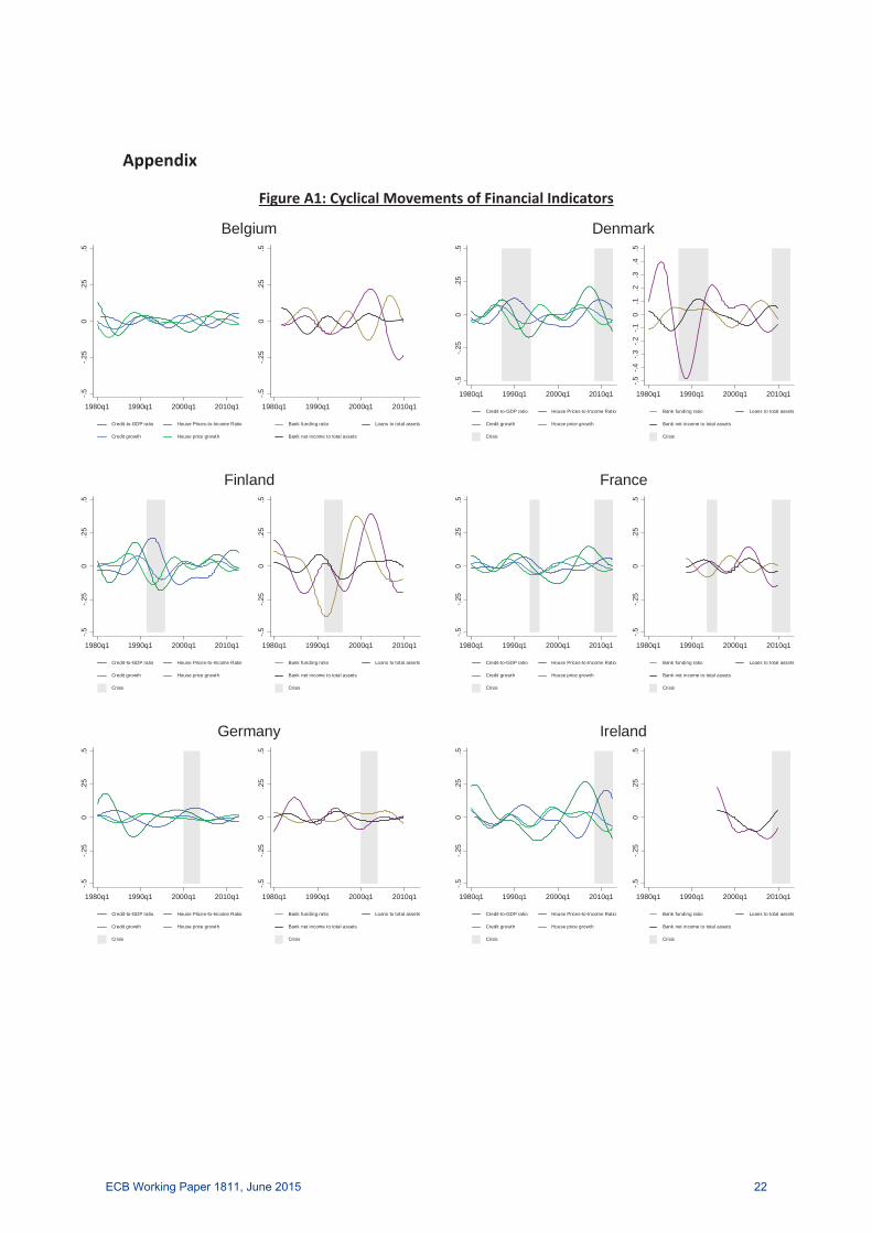
In the first step, we develop medium term cyclical components for each of the six individualindicators: credit to GDP ratio, house prices to income ratio, credit growth, house pricegrowth, bank funding ratio, bank net income to total assets ratio and loans to total assetsratio. However, due to the data constraints not all series are available for all countries at allpoints in time. In Figure 1, we exemplify the patterns of individual cycles by illustrating themfor Sweden. The individual graphs of the cyclical movements of the seven financialindicators for the remaining countries suggest a similar conclusion and are provided in theAppendix (Figure A1). The grey shaded areas in the figures reflect financial crisis periodsidentified by the ESCB Heads of Research Group Banking Crises Database.

9 Comin and Gertler (2006) apply the settings of 2 and 32 quarters for business cycles. Alternatively, one mayargue to use these BP settings for medium frequency components by Comin and Gertler (2006). However bothlines of reasoning imply the same parameters. Like Drehmann et al. (2012), we restrict the upper bound to 30years due to the constrained data availability.


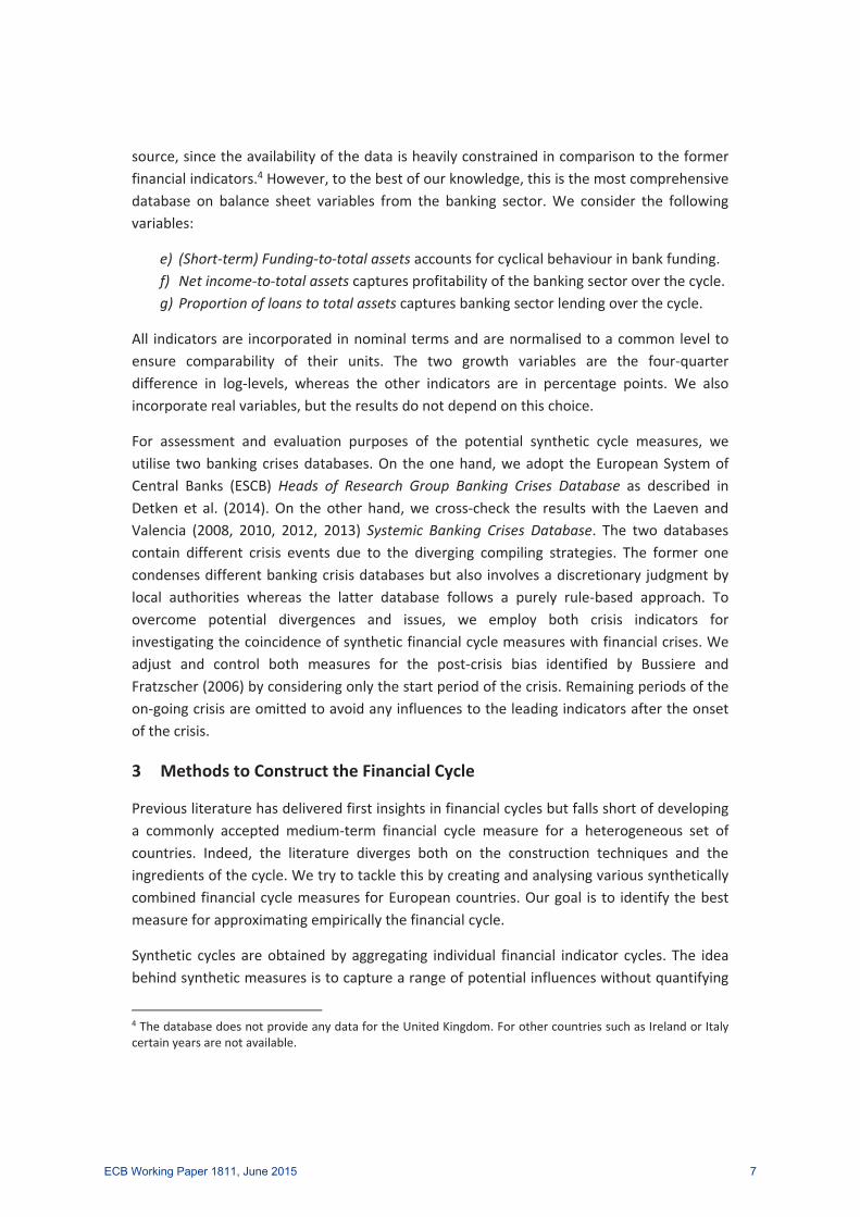
Figure 1: Cyclical Movements of Financial Indicators

The left panel of Figure 1 shows the cyclical components of the credit to GDP ratio, houseprices to income ratio, as well as credit growth and house price growth, whereas the rightpanel outlines the cyclical components of bank funding, loans to total assets and bank netincome to total assets ratios. Both panels help us to characterise the underlying indicatorsand to make statements about their potential usefulness. An obvious caveat of thisinvestigation is the limited number of full cycles incorporated in this time period.

The left panel reveals that cyclical components of credit aggregates and asset prices concurclosely. The peaks and troughs of the individual time series occur within a tight time frame.In addition, the frequencies of the time series are similar, whereas the amplitudes appear tobe divergent. Two of the four measures – both growth rates – tend to pick up quickly,whereas the other indicators adjust more gradually. In total, both growth rates tend tobehave as leading indicators, whereas the credit to GDP ratio seems to be rather a laggingone. All asset and credit indicators peak around the outbreak of financial distress in theearly 1990s and the late 2000s.

The data coverage in the right panel is a major concern and potential interpretations shouldbe drawn carefully considering that for some countries the available data is much moreconstrained (e.g. United Kingdom). The explanatory power and the concurrence of thebanking sector variables tend to diverge among countries. The frequencies but also theamplitudes appear to be different. In detail, for Sweden the peaks of the individual series inthe right panel are less closely aligned than in the left panel. The funding and income ratiospick up the development more quickly than the loans to total assets ratio. In comparison toasset prices and credit aggregates, banking variables are lagging and feature higheramplitudes.


Combining both panel interpretations, the graphical investigation reveals that variablescapturing asset prices and credit aggregates are more suitable for visualising cyclicalpatterns of the financial variables than banking sector variables.

These results provide a first indication of the relative importance of individual financialindicators for characterising the financial cycle. However, the validity of these cyclicalmovements is limited because single measures may miss certain developments in thefinancial markets. Accordingly, we construct cycle measures for the whole financial sector.Since no obvious financial cycle measure is available, we derive synthetic measures. Ofcourse, synthetic financial cycles have to be checked for their appropriateness beforedrawing any conclusion. Due to the favourable characteristics of frequency based filterseries, we are able to create aggregated synthetic financial cycle measures by averaging theunderlying frequency based filtered individual cycles for each point in time.10

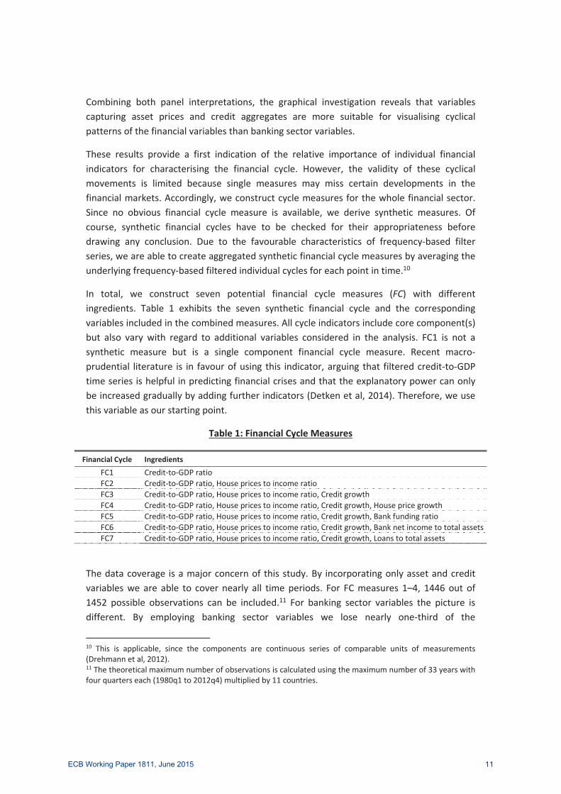
In total, we construct seven potential financial cycle measures (FC) with differentingredients. Table 1 exhibits the seven synthetic financial cycle and the correspondingvariables included in the combined measures. All cycle indicators include core component(s)but also vary with regard to additional variables considered in the analysis. FC1 is not asynthetic measure but is a single component financial cycle measure. Recent macroprudential literature is in favour of using this indicator, arguing that filtered credit to GDPtime series is helpful in predicting financial crises and that the explanatory power can onlybe increased gradually by adding further indicators (Detken et al, 2014). Therefore, we usethis variable as our starting point.

Table 1: Financial Cycle Measures

Financial Cycle Ingredients

FC1 Credit to GDP ratioFC2 Credit to GDP ratio, House prices to income ratioFC3 Credit to GDP ratio, House prices to income ratio, Credit growthFC4 Credit to GDP ratio, House prices to income ratio, Credit growth, House price growthFC5 Credit to GDP ratio, House prices to income ratio, Credit growth, Bank funding ratioFC6 Credit to GDP ratio, House prices to income ratio, Credit growth, Bank net income to total assetsFC7 Credit to GDP ratio, House prices to income ratio, Credit growth, Loans to total assets

The data coverage is a major concern of this study. By incorporating only asset and creditvariables we are able to cover nearly all time periods. For FC measures 1–4, 1446 out of1452 possible observations can be included.11 For banking sector variables the picture isdifferent. By employing banking sector variables we lose nearly one third of the

10 This is applicable, since the components are continuous series of comparable units of measurements(Drehmann et al, 2012).11 The theoretical maximum number of observations is calculated using the maximum number of 33 years withfour quarters each (1980q1 to 2012q4) multiplied by 11 countries.


observations. We are able to include for FC measure 4–7 only 1019, 1076 and 1076observations, respectively. Based on this coverage restriction, it would be advisable toemploy one of the former four financial cycle measures to ensure a wider data coverage.However, we assess and compare all different financial cycle measures in our analysis.

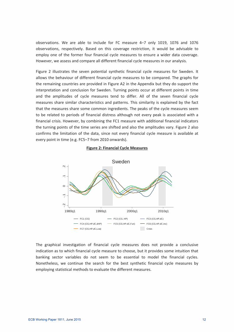
Figure 2 illustrates the seven potential synthetic financial cycle measures for Sweden. Itallows the behaviour of different financial cycle measures to be compared. The graphs forthe remaining countries are provided in Figure A2 in the Appendix but they do support theinterpretation and conclusion for Sweden. Turning points occur at different points in timeand the amplitudes of cycle measures tend to differ. All of the seven financial cyclemeasures share similar characteristics and patterns. This similarity is explained by the factthat the measures share some common ingredients. The peaks of the cycle measures seemto be related to periods of financial distress although not every peak is associated with afinancial crisis. However, by combining the FC1 measure with additional financial indicatorsthe turning points of the time series are shifted and also the amplitudes vary. Figure 2 alsoconfirms the limitation of the data, since not every financial cycle measure is available atevery point in time (e.g. FC5–7 from 2010 onwards).

Figure 2: Financial Cycle Measures

The graphical investigation of financial cycle measures does not provide a conclusiveindication as to which financial cycle measure to choose, but it provides some intuition thatbanking sector variables do not seem to be essential to model the financial cycles.Nonetheless, we continue the search for the best synthetic financial cycle measures byemploying statistical methods to evaluate the different measures.

-.2-.1

0.1

.2

1980q1 1990q1 2000q1 2010q1

FC1 (CG) FC2 (CG, HP) FC3 (CG,HP,dC)

FC4 (CG,HP,dC,dHP) FC5 (CG,HP,dC,Fun) FC6 (CG,HP,dC,Inc)

FC7 (CG,HP,dC,Loa) Crisis

Sweden


5 Assessment/Evaluation

The previous section focused on the graphical investigation in order to identify the bestfinancial cycle measure. In this section we extend the analysis by employing statisticalmethods to assess the various measures and to determine the best financial cycle measure.On the one hand, we analyse the concordance of the financial cycle measures and theiringredients. On the other hand, we explore the fitting of the financial cycle measures byinvestigating the development of synthetic cycle measures with regard to the outbreak offinancial crises.

In the first step, we investigate the synchronicity between the cyclical characteristics offinancial cycle ingredients and the aggregated financial cycle measures. For this purpose weuse a bivariate index of synchronisation, called the concordance index. This statisticalmeasure was developed by Harding and Pagan (2002). Basically, it expresses the timeperiods in which two time series are in the same phase in relation to all periods. If both timeseries are expanding or contracting, the index will be at 100% (positively concorded). Incases when the series are in different phases, the concordance measure is zero (negativelyconcorded).

Table 2: Concordance Measures for Medium term Cycles

Cycle Measure FC1 FC2 FC3 FC4 FC5 FC6 FC7

Concordance 100% 79% 76% 73% 74% 67% 72%

Table 2 exhibits the concordance measures for the ingredients of the financial cycle and itssynthetic financial cycle measure. Each number reflects the average of the underlyingconcordance measures of the synthetic financial cycle measure and its corresponding timeseries. More specifically, it represents the fraction of time in which the individual underlyingtime series components and the corresponding financial cycle share a common phase. Thefinancial cycle measures FC2 and FC3 show very distinctive values in the concordance indexindicating a close co movement of the financial cycle ingredients and that the synchronicityof the individual ingredients with the synthetic financial cycles is high. Other cycle measurestend to be less harmonised. Moreover, it is worth noting that the credit to GDP ratio seemsto be in comparison to other ingredients less concorded with the financial cycle. Typically,the concordance is around 50 60% for the credit to GDP ratio, whereas the concordanceindex of other indicators is considerably higher.12

In the next step, we explore the relationship between financial cycles and financial crises. Indetail, we study the coincidence and timing of a financial cycle’s peak and the outbreak of a

12 This finding may also deliver some insight that cyclical movements can be grouped into leading and laggingparameters. As noted in Section 4, the growth rates of credit and house prices seem to act as leadingindicators in our sample. The credit to GDP ratio seems to act rather as a lagging indicator.


financial crisis. It is important to stress that we do not attempt to forecast crises as in earlywarning literature. Therefore, we restrain from employing usefulness measures orspecifying any policy loss function which is typically used in this type of literature to gaugethe model’s predictive ability (e.g. Alessi and Detken (2011), Detken et al. (2014)). Rather,we are interested in evaluating the goodness of fit properties of financial cycle measures inan early warning framework.

In the spirit of Bush et al. (2014), we utilise the well established statistical measure “AreaUnder the Receiver Operating Characteristic” (AUROC) to assess the goodness of fit of eachfinancial cycle specification (e.g. Detken et al. (2014), Drehmann and Juselius (2014),Drehmann and Tsatsaronis (2014), Giese et al. (2014)). This technique does not require anyassumption on possible threshold values and weights of the signal ratio against the noiseratio. The AUROC summary statistics are bounded between 0 and 1, whereas higher AUROCvalues reflect more informative models. A value of 1 would represent a perfect fit, whereasa value below 0.5 corresponds with an uninformative specification.

In line with the dominating strand of the macro prudential literature, we employ a simplisticunivariate standard panel logistic model approach.13

.

In turn, we incorporate two financial crisis variables Heads of Research Group Banking CrisesDatabase by the ESCB and Systemic Banking Crises Database by Laeven and Valencia as thedependent Crisis variable. As independent variables we include a constant term C and onesynthetic financial cycle measure FC at a time. Our estimation procedure involves multiplesteps. To determine the power of each financial cycle measure in explaining crisis events,we estimate the specification for each financial cycle measure separately. Furthermore, weconsider 13 consecutive time horizons. We specify for each synthetic financial cyclemeasure a separate model, lagging the independent variable up to 3 years (12 quarters). Intotal, we estimate 12 regressions for each financial cycle measure. For each specification,we determine the AUROC which allows us to judge the model’s adequacy and the goodnessof fit. We repeat this estimation procedure for both measures.14

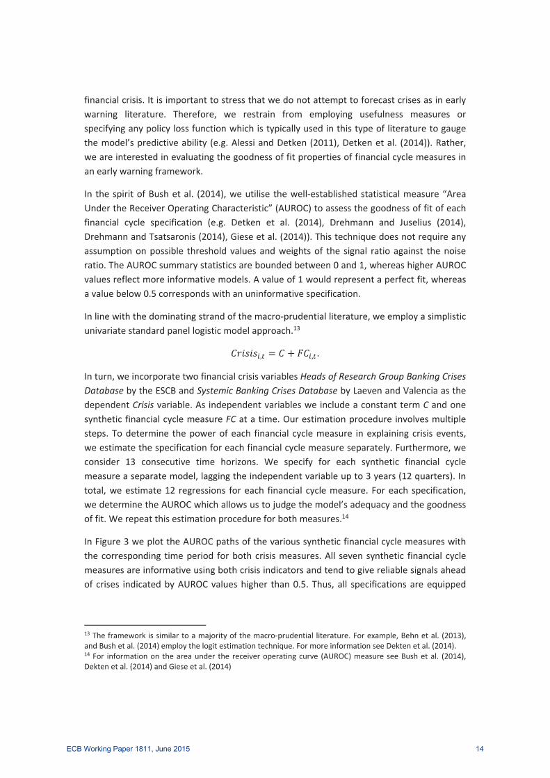
In Figure 3 we plot the AUROC paths of the various synthetic financial cycle measures withthe corresponding time period for both crisis measures. All seven synthetic financial cyclemeasures are informative using both crisis indicators and tend to give reliable signals aheadof crises indicated by AUROC values higher than 0.5. Thus, all specifications are equipped

13 The framework is similar to a majority of the macro prudential literature. For example, Behn et al. (2013),and Bush et al. (2014) employ the logit estimation technique. For more information see Dekten et al. (2014).14 For information on the area under the receiver operating curve (AUROC) measure see Bush et al. (2014),Dekten et al. (2014) and Giese et al. (2014)


with well behaving characteristics and are well determined. In particular, the higher theAUROC curve, the better is the performance of the model.

Figure 3: AUROC of Financial Cycle Measures Over Time

Both panels in Figure 3 show similar patterns. In both panels, the measures tend to behavequite similarly (except for FC1 and FC6) and it is challenging to distinguish between thevarious cycle measures as well as to identity the best performing measure. Nonetheless, thefigure reveals that specific financial cycles tend to be more informative than others. In theleft panel (Heads of Research Group Banking Crises Database) the FC3 and FC7 measureshave the highest AUROC values and can be described as the best performing models. In theright panel (Systemic Banking Crises Database) the FC2 and FC3 measures provide thehighest AUROC values. For both financial crisis measures, indicator FC3 is in the top ranksover all horizons and the value starts to decline slightly six quarters before the crisis. Incomparison, AUROC values of the FC1 measure which is the sole credit to GDP ratio declinesteadily with each further lag. In addition to that, it is observable that the explanatorypower of the financial cycle measures in terms of the AUROC value can be improved byadding further variables to the credit to GDP ratio. For example, in the left panel the AUROCvalue of the FC1 measure is much lower during the period of T( 12) until T( 3) than for theother cycle measures.

Taking the graphical and statistical examinations as well as the data availability concernsinto account, we conclude that the FC3 measure consisting of the credit to GDP ratio, creditgrowth and house prices to income ratio seems to be the best choice for a syntheticfinancial cycle measure. In comparison with other measures, this indicator is constantlyranked among the top in different graphical and statistical investigations.

6 Applications of the Financial Cycle Measure

After deriving the best fitting financial cycle indicator, we turn to some possible applicationsof the financial cycle measure. The synthetic financial cycle could be of help for variouspolicy purposes such as early warning indicators for detecting exuberance or distress within


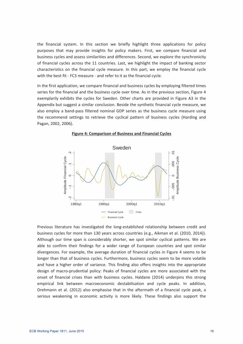
the financial system. In this section we briefly highlight three applications for policypurposes that may provide insights for policy makers. First, we compare financial andbusiness cycles and assess similarities and differences. Second, we explore the synchronicityof financial cycles across the 11 countries. Last, we highlight the impact of banking sectorcharacteristics on the financial cycle measure. In this part, we employ the financial cyclewith the best fit FC3 measure and refer to it as the financial cycle.

In the first application, we compare financial and business cycles by employing filtered timesseries for the financial and the business cycle over time. As in the previous section, Figure 4exemplarily exhibits the cycles for Sweden. Other charts are provided in Figure A3 in theAppendix but suggest a similar conclusion. Beside the synthetic financial cycle measure, wealso employ a band pass filtered nominal GDP series as the business cycle measure usingthe recommend settings to retrieve the cyclical pattern of business cycles (Harding andPagan, 2002, 2006).

Figure 4: Comparison of Business and Financial Cycles

Previous literature has investigated the long established relationship between credit andbusiness cycles for more than 130 years across countries (e.g., Aikman et al. (2010, 2014)).Although our time span is considerably shorter, we spot similar cyclical patterns. We areable to confirm their findings for a wider range of European countries and spot similardivergences. For example, the average duration of financial cycles in Figure 4 seems to belonger than that of business cycles. Furthermore, business cycles seem to be more volatileand have a higher order of variance. This finding also offers insights into the appropriatedesign of macro prudential policy: Peaks of financial cycles are more associated with theonset of financial crises than with business cycles. Haldane (2014) underpins this strongempirical link between macroeconomic destabilisation and cycle peaks. In addition,Drehmann et al. (2012) also emphasise that in the aftermath of a financial cycle peak, aserious weakening in economic activity is more likely. These findings also support the

-.01

-.005

0.0

05.0

1A

mpl

itude

Bus

ines

s C

ycle

-.2-.1

0.1

.2Am

plitu

de F

inan

cial

Cyc

le

1980q1 1990q1 2000q1 2010q1

Financial Cycle Crisis

Business Cycle

Sweden


intuition that dampening the financial cycle is an important element of policy measuresaiming at enhancing financial and macroeconomic stability as well.

In a second application, we analyse the synchronicity of financial cycles across the 11European countries. We define the cycle dispersion or synchronicity as the one year crosscountry standard deviation of filtered time series.15 This dispersion measure can be used toevaluate whether cycles converge or diverge over time. A lower dispersion measurerepresents a higher synchronicity and, vice versa, a lower synchronicity constitutes a higherdispersion.

Figure 5: Synchronicity of Cycles

Figure 5 offers an important insight: In awakening of cross border financial stress events(darker shaded line and labelled as “Early 1980s recession”, “1987 stock market crash”,“Nordic banking crisis”, “European exchange rate mechanism crisis”, “Burst of the dotcombubble”, “Global financial crisis”) the financial cycle dispersion tends to decrease andfinancial synchronicity tends to increase.16 Or to put it the other way around, financial cyclesare less synchronised in good times.17 This divergence of financial cycles calls fordifferentiated and well targeted policy responses that take into account the cyclical positionof individual Member States.

In a third and last step, we shed light on the potential drivers of the financial cycleamplitude and its importance for macro prudential policy purposes. Based on the newly

15 There are multiple options to analyse and model the synchronicity of cycles. For a detailed review ondifferent synchronisation measures see Gächter et al. (2012, 2013).16 The different shading during the Global financial crisis refers to the European Debit Crisis.17 Straetmans (2014) also finds that cross asset crisis spill overs – co movement of stocks, bonds andcommodities prices – become more pronounced and thus diversifying portfolio risks becomes more difficultduring recessions. Straetmans (2014) defines recessions in relation to the business cycle.


available instruments within the Capital Requirements Regulation and Directive (CRR/CRDIV) framework in Europe, designated macro prudential authorities obtain the power toimplement and calibrate certain capital buffers. The financial sectors feature differentcyclical and structural characteristics across Member States, suggesting that capital buffersshould be calibrated and implemented differently. Moreover, the timing of introducingmacro prudential measures in the financial cycle appears to be a key question to minimiseunintended economic costs. From a financial stability perspective, awareness of the driversof the financial cycle as well as its current state is essential to determine the adequate policyactions. For instance, our synthetic financial cycle measure could be employed as anindicator in the early warning system to assess countries’ financial sectors.

A detailed analysis of the relationship between certain structural features of the bankingsector and the financial cycle is undertaken by Stremmel and Zsámboki (2015). The authorsidentify bank concentration, the market share of foreign banks as well as the share offoreign currency loans in total loans which explain a significant part of the variation of thefinancial cycle amplitude. In addition, they also argue that macro prudential measuresaddressing cyclical movements and structural characteristics of the banking system could beconsidered in combination.

7 Conclusion

In this paper we identify key ingredients for the financial cycle in Europe. We reviewconstruction techniques and contrast different financial indicators such as credit aggregates,asset prices and banking sector variables and create various synthetic financial cyclemeasures to guide our choice. Employing various graphical and statistical assessments, weidentify the most appropriate financial cycle measures. Our results suggest that the bestfitted synthetic financial cycle measure contains the credit to GDP ratio, credit growth andhouse prices to income ratio.

Moreover, our paper elaborates on different potential applications of the financial cyclemeasure, contributing to the on going discussion on macro prudential policy. Awareness ofthe drivers of the financial cycle as well as its current state is essential to take the correctpolicy actions. We investigate the synchronicity of financial cycles in Europe. Our resultssuggest that financial cycles are highly correlated during stress times and diverge in boomperiods that should be taken into account in policy actions.

Further, we provide examples for potential application of the financial cycle measure. Thispaper paves the way for further avenues of research. From a research perspective it may beinteresting to further elaborate on the decomposition of financial cycles and whether therelative influence of individual components varies over time. In addition, our study providesalso the foundation to employ the financial cycle measures in other econometricframeworks. A possible application could involve using the financial cycle measures in VARmodels to conduct impact studies. Another interesting application is related to early


warning systems. This financial cycle metric could be employed in the early warningframework to assess the cyclical position of financial systems in countries and to issuesignals if emerging vulnerabilities are detected.


ReferencesAIKMAN, D., A.G. HALDANE and B. NELSON (2010): “Curbing the Credit Cycle”, Speech given at the Columbia University

Center on Capitalism and Society Annual Conference, New York, November.AIKMAN, D., A.G. HALDANE and B. NELSON (2014): “Curbing the Credit Cycle”, The Economic Journal, forthcoming.AIZENMAN, J., B. PINTO and S. VLADYSLAV (2013): "Financial Sector Ups and Downs and the Real Sector in the Open

Economy: Up by the Stairs, Down by the Parachute", Emerging Markets Review, 16(C), 1–30.ALESSI, L. and C. DETKEN, (2011): “Real Time Early Warning Indicators for Costly Asset Price Boom/Bust Cycles: A Role

for Global Liquidity”, European Journal of Political Economy, 27(3), 520–33.BASEL COMMITTEE ON BANKING SUPERVISION (BCBS) (2010): “Guidance for National Authorities Operating the

Countercyclical Capital Buffer”, Available at http://www.bis.org/publ/bcbs187.pdf.BASEL COMMITTEE ON BANKING SUPERVISION (BCBS) (2011): “Basel III: A Global Regulatory Framework for more

Resilient Banks and Banking Systems”, Available at http://www.bis.org/publ/bcbs189.pdf.BEHN, M., C. DETKEN, T. PELTONEN, and W. SCHUDEL (2013): “Setting Countercyclical Capital Buffers Based on Early

Warning Models: Would it Work?”, ECB Working Paper, No 1604.BORIO, C. and P. LOWE (2002): “Assessing the Risk of Banking Crises”, BIS Quarterly Review, December 2002, 43–54.BORIO, C. and P. LOWE (2004): “Securing Sustainable Price Stability, Should Credit Come back from the Wilderness?”,

BIS Working Paper, No 157.BORIO, C. and M. DREHMANN (2009): “Assessing the Risk of Banking Crises – Revisited”, BIS Quarterly Review, March

2009, 29–46.BORIO, C. (2012): “The Financial Cycle and Macroeconomics: What Have We Learnt?“, BIS Working Paper, No 395.BORIO, C. (2013): “Macroprudential Policy and the Financial Cycle: Some Stylized Facts and Policy Suggestions”, Speech

given at the “Rethinking Macro Policy II: First Steps and Early Lessons” hosted by the IMF in Washington, DC.BORIO, C., P. DISYATAT, and M. JUSELIUS (2013): “Rethinking Potential Output: Embedding Information about the

Financial Cycle”, BIS Working Paper, No 404.BRACKE, P. (2013): "How Long Do Housing Cycles Last? A Duration Analysis for 19 OECD Countries", Journal of Housing

Economics, 22, 213–30.BRY, G. and C. BOSCHAN (1971): “Cyclical Analysis of Time Series: Selected Procedures and Computer Programs”, NBER

Technical Paper, No 20.BURNS, A. F., and W. C. MITCHELL (1946): “Measuring Business Cycles”, Columbia Univ. Press.BUSCH, U. (2012): “Credit Cycles and Business Cycles in Germany: A Comovement Analysis”, Manuscript.BUSH, O., R. GUIMARAES and H. STREMMEL (2014): “Beyond the Credit Gap: Quantity and Price of Risk Indicators for

Macro–Prudential Policy”, Bank of England, Manuscript.BUSSIÈRE, M. and M. FRATZSCHER (2006): “Towards a New Early Warning System of Financial Crisis”, Journal of

International Money and Finance 25(6), 953–73.CHRISTIANO, L. and T. FITZERALD (2003): “The Band–Pass Filter”, International Economic Review, 44(2), 435–65.CLAESSENS, S., M. KOSE and M. TERRONES (2011a): “Financial Cycles: What? How? When?”, IMF Working Paper, No

WP/11/76.CLAESSENS, S., M. KOSE and M. TERRONES (2011b): “How Do Business and Financial Cycles Interact?”, IMF Working

Paper, No WP/11/88.COMIN, D. and M. GERTLER (2006): “Medium–Term Business Cycles”, American Economic Review, 96(3), 523–51.DETKEN, C. and F. SMETS (2004): "Asset Price Booms and Monetary Policy", ECB Working Paper, No 364.DETKEN, C., O. WEEKEN, L. ALESSI, D. BONFIM, M. M. BOUCINHA, C. CASTRO, S. FRONTCZAK, G. GIORDANA, J. GIESE,

N. JAHN, J. KAKES, B. KLAUS, J. H. LANG, N. PUZANOVA and P. WELZ (2014): “Operationalizing theCountercyclical Capital Buffer: Indicator Selection, Threshold Identification and Calibration Options”, ESRBOccasional Paper, 5.

DREHMANN, M., C. BORIO and K. TSATSARONIS (2011): “Anchoring Countercyclical Capital Buffers: The Role of CreditAggregates”, International Journal of Central Banking, 7(4), 189–240.

DREHMANN, M., C. BORIO and K. TSATSARONIS (2012): “Characterising the Financial Cycle: Don't Lose Sight of TheMedium Term!”, BIS Working Paper, No 380.

DREHMANN, M. and K. TSATSARONIS (2014): “The Credit–to–GDP Gap and Countercyclical Capital Buffers: Questionsand Answers”, BIS Quarterly Review, March 2014.

DREHMANN, M. and M. JUSELIUS (2014): “Evaluating Early Warning Indicators of Banking Crises: Satisfying PolicyRequirements“, International Journal of Forecasting, 30(3), 759 780.

ENGLISH, W, K. TSATSARONIS and E. ZOLI (2005): "Assessing the Predictive Power of Measures of Financial Conditionsfor Macroeconomic Variables", BIS Papers, No 22.

EUROPEAN SYSTEMIC RISK BOARD (ESRB) (2014): Macro prudential policy actions,https://www.esrb.europa.eu/mppa/html/index.en.html.


GÄCHTER,M., RIEDL, A. and D. RITZBERGER–GRÜNWALD (2012): "Business Cycle Synchronization in the Euro Area andthe Impact of the Financial Crisis", Monetary Policy & the Economy, Oesterreichische Nationalbank (AustrianCentral Bank), 2, 33–60.

GÄCHTER, M., RIEDL, A. and D. RITZBERGER–GRÜNWALD (2013):"Business Cycle Convergence or Decoupling?", BOFITDiscussion Paper, No 3/2013.

GERDRUP, K., A. KVINLOG and E. SCHAANNING (2013): “Key Indicators for a Countercyclical Capital Buffer in Norway– Trends and Uncertainty”, Norges Bank Staff Memo, No 13/2013.

GIESE, J., H. ANDERSEN, O. BUSH, C. CASTRO, M. FARAG, and S. KAPADIA (2014), “The credit to GDP gap andcomplementary indicators for macroprudential policy: Evidence from the UK”, International Journal ofFinance & Economics, 19(1), 25 47.

GOODHART, C and B HOFMANN (2008): "House Prices, Money, Credit, and the Macroeconomy", Oxford Review ofEconomic Policy, 24, 180–205.

HALDANE, A. (2014): “Ambidexterity”, Speech given at the 2014 American Economic Association Annual Meeting inPhiladelphia.

HANSEN, L. P.: “Challenges in Identifying and Measuring Systemic Risk”, NBER Working Paper, No 18505.HARDING, D. and A. PAGAN (2002): “Dissecting the Cycle: A Methodological Investigation”, Journal of Monetary

Economics, 49(2), 365–81.HARDING, D. and A. PAGAN (2006): "Synchronization of Cycles", Journal of Econometrics, 132, 59–79.HIEBERT, P., B. KLAUS, T. PELTONEN, Y. SCHÜLER and P. WELZ (2014): "Capturing the Financial Cycle in Euro Area

Countries", ECB Financial Stability Review – November 2014, Special Feature B.HODRICK, R. and E. PRESCOTT (1981): “Post–war U.S. Business Cycles: An Empirical Investigation”, Working Paper.

Reprinted in: Journal of Money, Credit and Banking (1997), 29(1), 1–16.KINDLEBERGER, C. P. (1978): “Manias, Panics, and Crashes: A History of Financial Crisis”, 1 , Basic Books.LAEVEN, L. and F. VALENCIA (2008): “Systemic Banking Crises: A New Database”, IM Working Paper, No 08/224.LAEVEN, L. and F. VALENCIA (2010): “Resolution of Banking Crises: The Good, the Bad, and the Ugly”, IMF Working

Paper, No 10/146.LAEVEN, L. and F. VALENCIA (2012): “Systemic Banking Crises Database: An Update”, IMF Working Paper, No 12/163.LAEVEN, L. and F. VALENCIA (2013): “Systemic Banking Crises Database”, IMF Economic Review 61 (2), 225 270.LESER, C. E. V. (1961): “A Simple Method of Trend Construction”, Journal of the Royal Statistical Society, Series B

(Methodological), 23, 91–107.LESER, C. E. V. (1963): “Estimation of Quasi–Linear Trend and Seasonal Variation”, Journal of the American Statistical

Association, 58, 1033–43.MINSKY, HYMAN P. (1972): “Financial Instability Revisited: The Economics of Disaster.” Reappraisal of the Federal

Reserve Discount Mechanism, 3, 97–136.MINSKY, HYMAN P. (1982): “The Financial Instability Hypothesis: Capitalistic Processes and the Behavior of the

Economy”, in “Financial Crises: Theory, History, and Policy”, Cambridge University Press, 12–29.MINSKY, HYMAN P. (1986): “Stabilizing an Unstable Economy”, Yale University Press.NG, T. (2011): “The Predictive Content of Financial Cycle Measures For Output Fluctuations”, BIS Quarterly Review,

June 2011, 53–65.RAVN, M. O. and H. UHLIG (2002): “On Adjusting the Hodrick–Prescott Filter for the Frequency of Observations”, The

Review of Economics and Statistics, 84(2), 371–80.SCHULARICK, M. and TAYLOR, A. M. (2012): “Credit Booms Gone Bust: Monetary Policy, Leverage Cycles and Financial

Crises, 1870–2008”, American Economic Review, 102(2), 1029–1061.STRAETMANS, S. (2014): “Financial Crisis, Crisis Spillovers and the Business Cycle”, Manuscript.STREMMEL, H. and B. ZSAMBOKI (2015). “The Relationship between Structural and Cyclical Features of the EU

Financial Sector”, ECB Working Paper Series, No 1812.UHDE, A. and U. HEIMESHOFF (2009): "Consolidation in Banking and Financial Stability in Europe: Empirical Evidence",

Journal of Banking & Finance, 33(7), 1299–1311.WEZEL, T. (2014): “Rightsizing the Countercyclical Capital Buffer for EU Countries – A Residual Loss Approach”,

European Central Bank, Manuscript.WHITTAKER, E. T. (1923): “On a New Method of Graduation”, Proceedings of the Edinburgh Mathematical Society,

41, 63–75.


Appendix

Figure A1: Cyclical Movements of Financial Indicators

-.5-.2

50

.25

.5

1980q1 1990q1 2000q1 2010q1

Credit-to-GDP ratio House Prices-to-Income Ratio

Credit growth House price growth

-.5-.2

50

.25

.5

1980q1 1990q1 2000q1 2010q1

Bank funding ratio Loans to total assets

Bank net income to total assets

Belgium

-.5-.2

50

.25

.5

1980q1 1990q1 2000q1 2010q1



Crisis

-.5-.4

-.3-.2

-.10

.1.2

.3.4

.5

1980q1 1990q1 2000q1 2010q1



Crisis

Denmark

-.5-.2

50

.25

.5

1980q1 1990q1 2000q1 2010q1



Crisis

-.5-.2

50

.25

.5

1980q1 1990q1 2000q1 2010q1



Crisis

Finland-.5

-.25

0.2

5.5

1980q1 1990q1 2000q1 2010q1



Crisis

-.5-.2

50

.25

.51980q1 1990q1 2000q1 2010q1



Crisis

France

-.5-.2

50

.25

.5

1980q1 1990q1 2000q1 2010q1



Crisis

-.5-.2

50

.25

.5

1980q1 1990q1 2000q1 2010q1



Crisis

Germany

-.5-.2

50

.25

.5

1980q1 1990q1 2000q1 2010q1



Crisis

-.5-.2

50

.25

.5

1980q1 1990q1 2000q1 2010q1



Crisis

Ireland


Each panel reflects the cyclical movements for seven different financial indicators. The cyclical movements are obtained using the described methodology in Section 3. Theleft part of each panel, represent the cyclic components of macro financial variables such as credit to GDP ratio, house prices to income ratio, credit growth, whereas theright part of each panel represents the cyclical components of banking balance variables such as bank funding, loans to total assets, and bank ne income to total assetsratios. This figure reveals that coverage of the banking sector balance sheet variables differs across the countries. For example, in the Italian case for some periods no data isavailable, whereas for the United Kingdom no balance sheet data is available at all. Other countries such as Spain have considerable higher data coverage. The grey shadedareas refer to financial crisis periods identified by ESCB Heads of Research Group Banking Crises Database for the corresponding country. For a detailed interpretation, please

see Section 4.

-.5-.2

50

.25

.5

1980q1 1990q1 2000q1 2010q1



Crisis

-.5-.2

50

.25

.5

1980q1 1990q1 2000q1 2010q1



Crisis

Italy

-.5-.2

50

.25

.5

1980q1 1990q1 2000q1 2010q1



Crisis

-.5-.2

50

.25

.5

1980q1 1990q1 2000q1 2010q1



Crisis

Netherlands

-.5-.2

50

.25

.5

1980q1 1990q1 2000q1 2010q1



Crisis

-.5-.2

50

.25

.5

1980q1 1990q1 2000q1 2010q1



Crisis

Spain

-.5-.2

50

.25

.5

1980q1 1990q1 2000q1 2010q1



Crisis

-.5-.2

50

.25

.5

1980q1 1990q1 2000q1 2010q1



Crisis

Sweden

-.5-.2

50

.25

.5

1980q1 1990q1 2000q1 2010q1



Crisis

-.5-.2

50

.25

.5

1980q1 1990q1 2000q1 2010q1



Crisis

United Kingdom


Figure A2: Financial Cycle Measures

Each country panels reflects seven constructed individual synthetic financial cycle measures. We use the following ingredients:FC1: Credit to GDP ratio (CG).FC2: Credit to GDP ratio (CG), House prices to income ratio (HP).FC3: Credit to GDP ratio (CG), House prices to income ratio (HP), Credit growth (dC).FC4: Credit to GDP ratio (CG), House prices to income ratio (HP), Credit growth (dC), House price growth (dHP).FC5: Credit to GDP ratio (CG), House prices to income ratio (HP), Credit growth (dC), Bank funding ratio (Fun).FC6: Credit to GDP ratio (CG), House prices to income ratio (HP), Credit growth (dC), Bank net income to total assets (Inc).FC7: Credit to GDP ratio (CG), House prices to income ratio (HP), Credit growth (dC), Loans to total assets (Loa).

Grey shaded areas reflect financial crisis periods identified by ESCB Heads of Research Group Banking Crises Database for the corresponding country. In line with Figure A1,for the United Kingdom the financial cycle measures FC5, FC6, and FC7 are not available due to the lack of balance sheet variables. For an interpretation of these countrypanels please see Section 4.

-.2-.1

0.1

.2

1980q1 1990q1 2000q1 2010q1



FC7 (CG,HP,dC,Loa)

Belgium

-.2-.1

0.1

.2

1980q1 1990q1 2000q1 2010q1




Denmark

-.2-.1

0.1

.2

1980q1 1990q1 2000q1 2010q1




Finland

-.2-.1

0.1

.2

1980q1 1990q1 2000q1 2010q1




France

-.2-.1

0.1

.2

1980q1 1990q1 2000q1 2010q1




Germany

-.2-.1

0.1

.2

1980q1 1990q1 2000q1 2010q1




Netherlands

-.2-.1

0.1

.2

1980q1 1990q1 2000q1 2010q1




Italy

-.2-.1

0.1

.2

1980q1 1990q1 2000q1 2010q1




Ireland

-.2-.1

0.1

.2

1980q1 1990q1 2000q1 2010q1




Sweden

-.2-.1

0.1

.2

1980q1 1990q1 2000q1 2010q1




Spain

-.2-.1

0.1

.2

1980q1 1990q1 2000q1 2010q1




United Kingdom


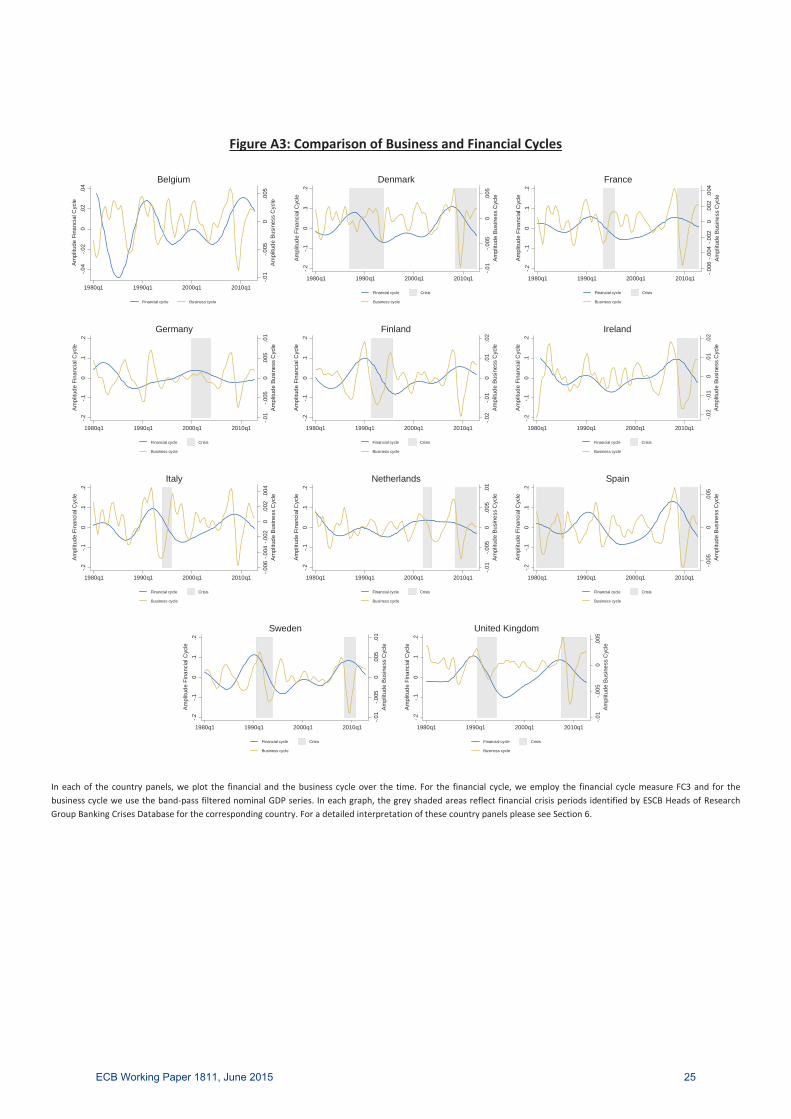
Figure A3: Comparison of Business and Financial Cycles

In each of the country panels, we plot the financial and the business cycle over the time. For the financial cycle, we employ the financial cycle measure FC3 and for thebusiness cycle we use the band pass filtered nominal GDP series. In each graph, the grey shaded areas reflect financial crisis periods identified by ESCB Heads of ResearchGroup Banking Crises Database for the corresponding country. For a detailed interpretation of these country panels please see Section 6.

-.01

-.005

0.0

05A

mpl

itude

Bus

ines

s C

ycle

-.04

-.02

0.0

2.0

4A

mpl

itude

Fin

anci

al C

ycle

1980q1 1990q1 2000q1 2010q1

Financial cycle Business cycle

Belgium

-.01

-.005

0.0

05A

mpl

itude

Bus

ines

s C

ycle

-.2-.1

0.1

.2A

mpl

itude

Fin

anci

al C

ycle

1980q1 1990q1 2000q1 2010q1

Financial cycle Crisis

Business cycle

Denmark

-.006

-.004

-.002

0.0

02.0

04A

mpl

itude

Bus

ines

s C

ycle

-.2-.1

0.1

.2A

mpl

itude

Fin

anci

al C

ycle

1980q1 1990q1 2000q1 2010q1


Business cycle

France

-.01

-.005

0.0

05.0

1A

mpl

itude

Bus

ines

s C

ycle

-.2-.1

0.1

.2A

mpl

itude

Fin

anci

al C

ycle

1980q1 1990q1 2000q1 2010q1


Business cycle

Germany

-.02

-.01

0.0

1.0

2A

mpl

itude

Bus

ines

s C

ycle

-.2-.1

0.1

.2A

mpl

itude

Fin

anci

al C

ycle

1980q1 1990q1 2000q1 2010q1


Business cycle

Finland

-.02

-.01

0.0

1.0

2A

mpl

itude

Bus

ines

s C

ycle

-.2-.1

0.1

.2A

mpl

itude

Fin

anci

al C

ycle

1980q1 1990q1 2000q1 2010q1


Business cycle

Ireland

-.006

-.004

-.002

0.0

02.0

04A

mpl

itude

Bus

ines

s C

ycle

-.2-.1

0.1

.2A

mpl

itude

Fin

anci

al C

ycle

1980q1 1990q1 2000q1 2010q1


Business cycle

Italy-.0

1-.0

050

.005

.01

Am

plitu

de B

usin

ess

Cyc

le

-.2-.1

0.1

.2A

mpl

itude

Fin

anci

al C

ycle

1980q1 1990q1 2000q1 2010q1


Business cycle

Netherlands

-.005

0.0

05A

mpl

itude

Bus

ines

s C

ycle

-.2-.1

0.1

.2A

mpl

itude

Fin

anci

al C

ycle

1980q1 1990q1 2000q1 2010q1


Business cycle

Spain

-.01

-.005

0.0

05.0

1A

mpl

itude

Bus

ines

s C

ycle

-.2-.1

0.1

.2A

mpl

itude

Fin

anci

al C

ycle

1980q1 1990q1 2000q1 2010q1


Business cycle

Sweden

-.01

-.005

0.0

05A

mpl

itude

Bus

ines

s C

ycle

-.2-.1

0.1

.2A

mpl

itude

Fin

anci

al C

ycle

1980q1 1990q1 2000q1 2010q1


Business cycle

United Kingdom


Acknowledgements

Hanno Stremmel

© European Central Bank, 2015

Postal addressTelephoneInternet

ISSNISBNDOIEU catalogue number

Working Paper Series - European Central Bank · 2015-06-17 · Working Paper Series Capturing the...

Documents

Transcript of Working Paper Series - European Central Bank · 2015-06-17 · Working Paper Series Capturing the...