8

No. 2012-09 April 2012

ISER W

orking Paper Series

ww

w.iser.essex.ac.uk

Disability costs and equivalence scales in the older population

Marcello Morciano University of East Anglia

Stephen Pudney

Ruth Hancock

Institute for Social and Economic Research University of Essex

University of East Anglia

Non-technical summary

Disabled people face higher costs of living than do non-disabled people. These additional costs include the cost of adapting the home, overcoming the difficulties of getting about, and acquiring assistance with everyday tasks that non-disabled people can do unaided. Countries like the UK have welfare benefit systems that acknowledge these costs through disability-tested programmes like Attendance Allowance (AA) and Disability Living Allowance (DLA). But just how large are these disability-related costs? How far does the benefit system go in meeting them? And how should we take account of these costs when we measure poverty and inequality in populations that include both disaabled and non-disabled people? In this research study, we construct dual indices of individuals’ standard of living and degree of disability, using UK survey data covering over 8,000 people who are over state pension age. We use these indices to estimate the additional income that each disabled person would need in order to reach the same standard of living as he or she would enjoy without any disability. There are two major empirical findings. (1) The additional costs of living associated with disability are large: among the group of people with some detectable degree of disability, we estimate the average cost to just under £100 per week, which is around 50% of their weekly income. As one would expect, the size of disability costs rises sharply with the severity of disability. (2) Although the disability benefits AA and DLA are well-targeted on people with significant disability, many disabled people do not receive them and, for those who do, they generally fall short of meeting the whole costs of disability. The average amount of benefit received by people with some disability is estimated at around £19, or less than a fifth of average costs. As a consequence of these findings, we can say that older disabled people primarily cope with disability costs by accepting a substantially reduced standard of living rather than by generating additional income through the benefit system. Our findings also underline the importance of taking account of disability-related living costs when drawing conclusions about poverty and inequality in the older population, where the prevalence of disability is particularly high.

DISABILITY COSTS AND EQUIVALENCE SCALES IN THE OLDER POPULATION

MARCELLO MORCIANO

RUTH HANCOCK Health Economics Group, University of East Anglia

STEPHEN PUDNEY Institute for Social and Economic Research, University of Essex

ABSTRACT: We estimate the implicit disability costs faced by older people, using data on over 8,000 individuals from the UK Family Resources Survey. We extend previous research by using a more flexible statistical modelling approach and by allowing for measurement error in observed disability and standard of living indicators. We find that disability costs are strongly related to the severity of disability and to income and – at an average level of almost £100 per week among over-65s with significant disability – they typically far exceed the value of any state disability benefits received.

KEYWORDS: costs of disability, disability indexes, standard of living, equivalence scale, structural equation modelling.

JEL CODES: C81, D1, I1.

CONTACT DETAILS: Marcello Morciano, Health Economics Group, Norwich Medical School, University of East Anglia, Norwich Research Park, Norwich, NR4 7TJ, UK (m.morciano@uea.ac.uk).

This work was supported by the Nuffield Foundation, by the Australian Research Council and by the Economic and Social Research Council through the Research Centre on Micro-social Change (MiSoC). Data from the Family Resources Survey (FRS) are made available by the UK Department of Work and Pensions through the UK Data Archive. Material from the FRS is Crown Copyright and is used by permission. Neither the collectors of the data nor the UKDA bear any responsibility for the analyses or interpretations presented here.

1

INTRODUCTION

Disabled people experience significant additional costs as a consequence of their

disability, and this is recognized in social security systems through the provision of

benefits designed to compensate for disability-related consumption costs. When

carrying out analysis of the distributional impact of tax-benefit reforms, it is crucially

important to make some allowance for these additional living costs, since failure to

do so would give a misleadingly favourable view of the position of disabled people

(Hancock and Pudney, 2010).

At least five different methods have been used to estimate and adjust for the costs of

disability. One is to exploit the existing benefit system and assume that the political

process has resulted in an acceptable evaluation of disability costs. This implies use

of an income measure for distributional analysis which excludes any receipt of

disability benefit (see Hancock and Pudney, 2010, Morciano et al., 2010), on the

assumption that income from disability benefit is exactly offset by the extra costs of

disability. However, in practice such payments follow simple rules not well tailored

to each individual’s specific configuration of impairments and they are not

necessarily intended to meet the full costs of disability. There may also be

imperfections in the eligibility judgements made by programme administrators and

non take-up by potential claimants. Consequently, this approach may give a poor

approximation to disability costs, with underestimation in many cases, leading to bias

in the distributional analysis.

A second, judgement-based, approach attempts to estimate the disability costs by

asking a panel of ‘experts’, or disabled people themselves, to identify disability-

related costs: see Martin and White, 1988, Thompson et al., 1990, Smith et al., 2004

for examples of this approach. The difficulty here is that the appropriate costs may

depend not only on the nature of the impairments suffered by the individual, but also

other characteristics that vary across households, and it is not feasible to use expert

judgement at the level of individual respondents to large-scale surveys. Disabled

people themselves may also find it difficult to envisage and evaluate the

counterfactual situation in which their disability is removed but all else remains

constant.

2

A third ‘objective’ revealed preference approach constructs an equivalence scale by

using the consumption pattern (typically the household’s food budget share) as an

indicator of living standards in a comparison of a sample of disabled people with

matched individuals who are unaffected by disability. This has been done extensively

in the context of adjustment for household size and structure, but less often for

disability (although see Jones and O’Donnell, 1995 for a UK example). The main

difficulty with this revealed preference method is the need for strong assumptions to

overcome inherent identification problems (Pollack and Wales 1979; Muellbauer

1979; Coulter et al., 1992; Banks et al., 1997; Deaton and Paxson, 1998).

A fourth alternative is to use a ‘subjective’ equivalence approach, based on

individuals’ reported satisfaction with their well-being. Two main types of subjective

information have been used: evaluations of standard of living using an arbitrary

numerical scale; or judgements on the level of income believed necessary to reach a

specified standard of living (see Stewart, 2009). For the subjective approach, there

are concerns about the quality of subjective assessments and the failure to address

problems caused by measurement error.

In this paper, we pursue a fifth and less widely-used Standard of Living (SoL)

approach which lies somewhere between these last two approaches. The method is

closely related to work on material deprivation which seeks to expand the concept of

poverty beyond conventional income- or consumption-based constructs (see

Berthoud et al., 1993; Zaidi and Burchardt, 2005; Cullinan et al., 2011). We assume

that disabled people, in diverting resources to goods and services which are required

because of disability, experience a lower SoL than their non disabled counterparts.

The absolute costs of disability can be identified as the additional income required by

a disabled person to reach the same SoL as a non disabled person, holding constant

other characteristics, and the relative cost is the ratio of this amount to income. As

Zaidi and Burchardt (2005) point out, estimates depend on the choice of a suitable

standard of living indicator and the form of its relationship to income and disability

status.

Our aim is to develop and improve the method further in two important respects.

First, we allow for a more flexible relationship between income and SoL, so that the

structure of the estimated disability cost and equivalence scale is not dictated by an

unduly restrictive functional form assumption. Second, we address the problem of

3

measurement error in disability and SoL. Both SoL and disability status are typically

measured using either a binary classification or a count index based on a range of

different questionnaire items1. Although sensitivity analyses are often used to assess

robustness, this is not effective if all the alternatives entail similar measurement error

biases. To address this we use a latent factor model for disability and SoL, which

explicitly allows for the existence of measurement errors in the observable

indicators.

Using a two-latent factor structural equation model we estimate the extra cost of

disability for a representative sample of people over state pension age living in

private households in Great Britain, who were interviewed in the 2007/8 Family

Resources Survey (FRS). Ten indicators of ability to afford particular items or

activities are used to construct a latent continuous index of SoL. The latent SoL is

modelled as a function of income, (latent) disability, and other characteristics, which

reflect the many factors which determine an individual’s achieved standard of living.

In line with previous work (Morciano et al., 2010), disability is assumed to be a

latent concept which can be measured imperfectly by a vector of survey indicators

reflecting difficulties in domains of life and is influenced by observed socio-

economic and demographic characteristics of the individual.

This paper is organized as follow. Section 2 briefly describes the standard of living

approach and its usage. Section 3 presents the latent-factor structural equation

framework we employ. Section 4 describes the data used. Section 5 presents

estimates of the structural equation model and derives the associated estimated extra

costs of disability. Section 6 reports some sensitivity analysis on the initial results.

The final section draws conclusions.

1. THE STANDARD OF LIVING METHOD

Berthoud (1991) reviews various early attempts at conceptualizing and quantifying

how standard of living (SoL), income and disability are related. Berthoud et al.

(1993) and Zaidi and Burchardt (2005) formalized this approach, which has been

1 The Katz activities of daily living (Katz et al., 1963) and Barthel indices (Mahoney and Barthel, 1965) are two widely used tools for assessing ability to perform activities of daily living. These indices assign scores to self-reported degrees of difficulty in performing a number of activities, such as feeding, dressing, moving, bathing etc. Scores for each item are then aggregated. These indices have been criticized for the way reported difficulties are aggregated and for not taking account of potential measurement errors in self-reported difficulties (Feinstein et al., 1986; Hartigan, 2007).

4

used also by Saunders (2007) and Cullinan et al. (2011) for estimating the cost of

disability in Australia and Ireland respectively. The SoL approach is illustrated in

Figure 1, where we compare a positive level of disability D with the baseline of non-

disability, D0.

FIGURE 1

Standard of Living, Income and Disability

The two curves plot the relation between income and SoL conditional on disability,

and are assumed to increase monotonically with income. For any given value of

income, the SoL of the disabled person lies below that of the non-disabled person

and the vertical distance AC measures the difference in their standards of living at

the level of income Y. This measure is essentially Sen’s concept of “conversion

handicap” (Doessel and Whiteford, 2004). The horizontal distance AB provides a

measure of the extra income (∆) required to bring the SoL of the disabled person up

to the same level as the non-disabled person.

To formalise this idea, consider the following additively separable SoL function:

𝑆 = 𝑓(𝑌) − 𝑔(𝐷) + ℎ(𝑋, 𝜀) (1)

where S is the SoL, Y is a measure of financial resources, D is the degree of disability

status and 𝑋 and 𝜀 represent other observable and unobservable individual

characteristics. Some individuals may be in receipt of disability benefit (B), others

may not. To allow for this, we decompose income as:

𝑌 = 𝑌0 + 𝐵 (2)

5

where 𝑌0 excludes disability benefits. Now define a reference level of disability 𝐷0

and assume that the reference non-disabled person receives no disability benefit. We

now pose the following question: what is the smallest amount of additional income,

over and above 𝑌0, that would be needed for a person with disability level 𝐷 to

achieve the same SoL as he or she would have with income 𝑌0 and disability reduced

to the reference level 𝐷0? Given the additivity of (1), this additional income need, Δ,

is independent of 𝑋 and 𝜀, and solves the following optimisation problem:

min Δ subject to: 𝑓(𝑌0 + Δ) − 𝑔(𝐷) ≥ 𝑓(𝑌0) − 𝑔(𝐷0) (3)

In general, the total disability-induced living cost Δ and the associated proportional

equivalence scale 𝜎 = (𝑌0 + Δ)/𝑌0 depend on the levels of both income 𝑌0 and

disability.

For the cost Δ to depend only on severity of disability D (as implied by the design of

some benefit systems), the income-SoL profile must have the linear form 𝑓(𝑌0) =

𝛾1𝑌0, in which case the cost of disability and associated equivalence scale are:

Δ = [𝑔(𝐷) − 𝑔(𝐷0)]/ 𝛾1; 𝜎 = 1 + [𝑔(𝐷) − 𝑔(𝐷0)]/𝑓(𝑌0) (4)

For the equivalence scale 𝜎 to depend only on disability would require 𝑓(𝑌0 + Δ) =

𝑓(𝜎𝑌0) to be expressible as 𝑓(𝑌0) + 𝑎(𝜎), for all positive 𝜎 and some function 𝑎(. ).

The only function satisfying this property is 𝑓(𝑌0) = 𝛾1ln(𝑌0), which implies the

following cost of disability and equivalence scale2:

Δ = 𝑌0 �𝑒𝑔(𝐷)−𝑔(𝐷0)

𝛾1 − 1� ; 𝜎 = 𝑒𝑔(𝐷)−𝑔(𝐷0)

𝛾1 (5)

This is the form usually adopted for equivalence scales designed to adjust for

demographic differences between households in conventional income inequality

analysis. Both the linear and log-linear specifications have the advantage of

simplicity and incorporate the property of base independence (or invariance of the

equivalence scale to income level) in additive or multiplicative form (Lewbel, 1997).

In addition to these standard forms, we also use a more flexible log-quadratic

function of the kind that has been found useful in Engel curve studies (Banks et al.,

1997) and embodies the constant- 𝜎 model as a special case. If 𝑓(𝑌0) is specified as:

2 Strictly speaking, f can be any affine transform of ln(𝑌0); but an additive translation has no effect.

6

𝑓(𝑌0) = 𝛾1ln(𝑌0) + 𝛾2[ln(𝑌0)]2 (6)

then the solution to (3) gives the cost of disability and equivalence scale as:

Δ = 𝑒𝑥𝑝 � −𝛾1 − �𝛾12 − 4𝛾2𝐶

2𝛾2 � − 𝑌0 (7)

𝜎 = 𝑌0−1 𝑒𝑥𝑝 �

−𝛾1 − �𝛾12 − 4𝛾2𝐶

2𝛾2 � (8)

where 𝐶 = −[𝛾1ln(𝑌0) + 𝛾2[ln(𝑌0)]2 + 𝑔(𝐷) − 𝑔(𝐷0)]. Note that this solution

requires the condition 𝐶 ≤ 𝛾12/4𝛾2 to be satisfied.

This emphasises the importance of the specification used to relate SoL to income and

the need to allow for the possibility of departures from the simple assumptions of

linear or log-linear forms.

2. A STATISTICAL MODEL

We use the following two-latent factor simultaneous equation model:

𝑆𝑖𝑞 = 𝟏�𝜆𝑞𝜑𝑖 + 𝜁𝑖𝑞� (9)

𝐷𝑖𝑘 = 𝟏(𝜇𝑘𝜂𝑖 + 𝜉𝑖𝑘) (10)

𝜑𝑖 = 𝑓(𝑌𝑖;𝜸) + 𝛼1𝜂𝑖 + 𝜶2𝒙𝑖 + 𝜀1𝑖 (11)

𝜂𝑖 = 𝜷𝒛𝑖 + 𝜀2𝑖 (12)

where i denotes sampled individuals (i = 1 ... N), 𝑓(. ) represents the linear, log-

linear or log-quadratic function and 𝜸 contains the corresponding coefficients. The

latent measure of SoL is φi which underlies the observed SoL indicators Si1...SiQ , and

the latent disability index ηi generates observed disability indicators Di1...DiK. The

parameters qλ and kµ are factor loadings associated with the Siq and Dik indicators

respectively. iqζ and ikξ are the measurement errors associated with the SoL and

disability indicators. The indicator function 1(.) maps the latent indexes on the right-

hand side of the measurement equations (9) and (10) into the observed binary

indicators of SoL and disability.

7

Observable covariates representing personal characteristics and household

circumstances appear in vectors ix and iz . They contain socio-economic and

demographic influences on living standards and disability respectively. In this model

socio-economic factors have both a direct and an indirect effect on SoL. Income, for

example, has the direct effect of increasing resources available for consumption; this

is captured by the function 𝑓(𝑌𝑖;𝜸). Income also has an indirect influence on

disability, through the term 𝜷𝒛𝑖, which then increases disability-related costs through

the term 𝛼1𝜂𝑖. The use of a latent disability model allows us to separate these direct

and indirect effects. Note that the income concepts relevant to the direct and indirect

paths are different. The direct effect involves current resources available for

consumption, which includes receipt of disability benefit. In contrast, modeling of

the indirect effect requires a long-term concept of economic resources reflecting the

cumulative effect of past living standards on the current health state. Since disability

precedes the receipt of disability benefit, it follows that the latter should be excluded

from the income variable used to capture the indirect causal path.

Identification is achieved by imposing the assumption that the structural errors 1ε

and 2ε are uncorrelated and their scale is normalised by setting var( 1ε )= var( 2ε )=1.

We also make the conventional assumption that the measurement errors iqζ and ikξ

are independent. Because the normalisation results in arbitrary scales for φ and η, we

present coefficient estimates for equation (11) in an alternative standardized version.

The variance of the latent SoL index in (11) is 𝑣𝑎𝑟(𝑓(𝑌𝑖;𝜸) + 𝛼1𝜂𝑖 + 𝜶2𝒙𝑖) + 1 =

�1 − 𝑅𝜑2�, where Rφ2 is the squared multiple correlation of φ. Switching to a

standardised version of φ would then multiply each coefficient by a factor �1 −

𝑅𝜑2−1/2 and this renormalized coefficient is interpretable as the change in φ in

standard deviation units, produced by a 1-unit increase in the value of the covariate.

Disability η is also a latent construct, with variance 𝑣𝑎𝑟(𝜷𝒛𝑖) + 1 = �1 − 𝑅𝜂2�,

where 𝑅𝜂2 is the squared multiple correlation of the disability equation. Therefore the

standardized coefficient of φ on η is 𝛼1𝑆𝑇𝐷 = 𝛼1���1 − 𝑅𝜂2� �1 − 𝑅𝜑2�� �, which can

be interpreted as the change in φ (in standard deviation units) generated by a 1-

standard deviation increase in η.

8

3. DATA

The data are taken from the 2007-08 Family Resources Survey (FRS). The FRS is a

large UK household survey which collects very detailed incomes and assets

information from respondents and asks them questions covering a range of

difficulties due to health or disability problems. Additionally, the survey includes a

series of questions aimed at measuring material deprivation (Department for Work

and Pensions, 2009). For this paper we restrict the analysis to households in Great

Britain where all members are aged over state pension age (65 for men; 60 for

women) and the household contains only a single person or a couple. The age

restriction is imposed in order to limit endogeneity bias which may arise for younger

adults for whom disability may cause a reduced income by limiting labour market

participation3. In estimating equations (11) and (12) we measure income at the

household level assuming that all members of the households benefit to the same

extent from total household income. This is less likely to be true for households

which contain members other than a single or couple pensioner who are therefore

excluded. After dropping a few cases where relevant information is missing the

resulting sample contains 8,183 individuals (5,812 households). About 58% of the

sample are partnered and the remainder live alone.

Deprivation indicators are derived from a set of questions about items or activities,

seen as potential ‘necessities’, that households have or do; households who did not

have the items or do the activities were asked whether this was because they did not

want them or because they could not afford them. From these household-level

indicators, we created individual-level indicators in which each household member is

assigned the values of the deprivation indicators of their household. Each such

indicator is set equal to 1 if the respondent answered “We/I would like to have this

but cannot afford this at the moment” and 0 otherwise. It has been suggested

(McKay, 2004, 2008; Berthoud et al., 2009) that certain segments of the population

with lowered expectations, such as disabled older people, may be less likely than

others to admit to being unable to afford particular activities or goods. We therefore

carry out a sensitivity analysis in which the deprivation indicator is set to 1 if the

household does not do or have the activity/good in question, irrespective of whether

3 For a discussion on this point we refer, amongst others, to Goldman (2001) and Adams et al. (2003).

9

they say that is because they cannot afford or they do not want them. Sample

statistics corresponding to the two alternative definitions of deprivation are shown in

Table 1.

Table 1 Sample means and standard deviations (in brackets) of the deprivation indicators

Do you (and your family/and your partner) have... Cannot afford to… Do not want/ have / or

cannot afford to …

Enough money to keep your home in a decent state of decoration? 0.083 (0.276) 0.101 (0.302)

Hobby or leisure activity? 0.036 (0.187) 0.254 (0.435)

Holidays away from home one week a year? 0.162 (0.368) 0.436 (0.496)

Household contents insurance? 0.049 (0.217) 0.109 (0.312)

Friends/family round for drink or meal at least once a month? 0.068 (0.252) 0.413 (0.492)

Make savings of £10 a month or more? 0.214 (0.41) 0.404 (0.491)

Two pairs of all-weather shoes for each person in the household? 0.022 (0.146) 0.038 (0.19)

Replace any worn out furniture? 0.153 (0.36) 0.323 (0.468)

Replace or repair broken electrical goods? 0.104 (0.306) 0.179 (0.383)

Money to spend each week on yourself, not on your family? 0.079 (0.27) 0.118 (0.322)

Notes: Sample means and standard deviation computed over a sample of 8,183 FRS 2007-8 respondents.

In estimating equations (9)-(12), we invert these deprivation indicators to construct

the SoL indicators, Si1...SiQ, which take the value 0 if the respondent cannot afford

the activity/good and 1 otherwise. In subsequent sensitivity analysis, they take the

value 0 if the respondent does not do/have the activity/good and 1 otherwise.

Respondents in the FRS are asked whether they have a health problem or disability.

If they answer ‘yes’ they are then asked if that means they have significant

difficulties in any of 9 areas of life. The list of disability indicators together with

their prevalence is reported in Table 2. Fifty-three per cent of the sample reported

having no disability; 20% reported having three or more difficulties. The most

common difficulties are those concerning physical impairment (difficulties in

mobility; with lifting, carrying or moving objects).

10

Table 2

Sample means and standard deviations of the disability indicators

Does this health problem(s) or disability(ies) mean that you have significant difficulties with any of these areas of your life? Please read out the numbers from the card next to the ones which apply to you.

Mean Standard Deviation

difficulty in mobility (moving about) 0.327 0.469

difficulty with lifting, carrying or moving objects 0.301 0.459

difficulty with manual dexterity using hands for daily tasks 0.120 0.325

difficulty - continence (bladder/bowel control) 0.071 0.256

difficulty with communication (speech, hearing or eyesight) 0.089 0.285

difficulty with memory/concentration/learning/understanding 0.063 0.242

difficulty with recognising when in physical danger 0.013 0.114

difficulty with your physical co-ordination 0.109 0.312

difficulty in other area of life 0.123 0.328

Notes: Statistics computed over a sample of 8,183 FRS 2007-8 respondents.

The explanatory covariates used in the SoL and disability equations are summarised

in Table 3. The income indicator Y used in the SoL equation represents the resources

of the household currently available for meeting the consumption needs of the

household members. We use a household-level income measure, net of direct taxes

and housing costs, in line with the “After Housing Cost” measure used in the official

Households Below Average Income analysis (DWP, 2009) and also by Zaidi and

Burchardt (2005). This measure includes income from investments (interest, rent,

dividends, private pensions, annuities) but, unlike Zaidi and Burchardt, our income

variable includes disability benefits since, as argued earlier, it is available, like any

other income component, to be used to maintain SoL (see also Stapleton, 2008 and

Cullinan et al., 2011). Disability benefits comprise the non-means-tested Attendance

Allowance and Disability Living Allowance4, an estimate of income attributable to

the Severe Disability Premium component5 of means-tested pensioner benefits and

4 Attendance Allowance is the main disability-related cash benefit available to people aged 65 or over in th UK. In 2007 it was £64.50 or £43.15 depending on level of care need. Disability Living Allowance is a similar benefit that must be claimed before age 65 but can continue to be paid beyond age 65. It has three alternative rates for care needs and three for mobility needs such that in 2007 weekly payments ranged from £17.75 to £109.50. 5 The Severe Disability Premium is worth up to £48.45 for an older disabled person receiving a means-tested benefit.

11

other minor disability-related benefits that are received by a small number of older

people in our sample.

Table 3 Sample means and standard deviations of covariates

Mean Standard Deviation

Age of adult last birthday 73.54 7.431

Female 59.2% 0.491

No. of yrs in FT education beyond school living age 1.02 1.676

Whether Partnered 58.0% 0.494

Area of Residence:

North East 4.6% 0.209

North West and Merseyside 10.9% 0.312

Yorks and Humberside 8.4% 0.277

East Midlands 7.5% 0.263

West Midlands 8.3% 0.276

Eastern 8.8% 0.283

London 6.9% 0.253

South East 12.2% 0.327

South West 8.7% 0.282

Wales 5.3% 0.225

Scotland 18.4% 0.387

Net household income including disability benefits but after deducting housing costs (£ pw)a

283.70 176.69

Net household income excluding disability benefits and after deducting housing costs (£ pw) (‘Pre-disability benefit income’)b

268.20 177.67

Home Ownership 75.1% 0.432

Financial wealth (in £) 20,886 63,376 Notes: Sample means computed over the 8,183 respondents. Monetary values are in 2007 prices and rounded to the nearest 10p. a. Computed as the sum across all household members of: cash income from private and state pensions, investments and savings, other market income, disability and means-tested state benefits minus income tax and housing costs. Housing costs are the sum of gross rents, council tax payments, costs of insurance on structure of property and mortgage interest payments net of housing benefit and council tax benefits. b. Pre-disability benefits income is computed by deducting disability benefits currently received by all household members from household income.

The measure of income used as a covariate (in 𝒛) in the disability equation also

includes current income from investments, since interest, rent, dividends, private

pensions and annuities are returns on assets accumulated over the lifecycle and are,

consequently, good indicators of the past access to resources that exerts a cumulative

positive influence on health. For the same reason, we also include a measure of

12

financial wealth6 in the disability equation and a dummy variable to indicate home

ownership. Note that the income measure used as a covariate in the disability

equation excludes current receipt of disability benefits, since those are a

consequence, rather than a determinant, of current disability.

Rather than use an arbitrary equivalence scale to adjust income for household

composition, we include a dummy variable to indicate whether the household

contains a single person or a couple in the disability and SoL equations. In line with

previous work (Zaidi and Burchardt, 2005, Stewart, 2009), we also include a set of

personal characteristics including age, gender, level of education, home ownership

and marital status, together with regional dummies to reflect geographical differences

in cost of living and in health.

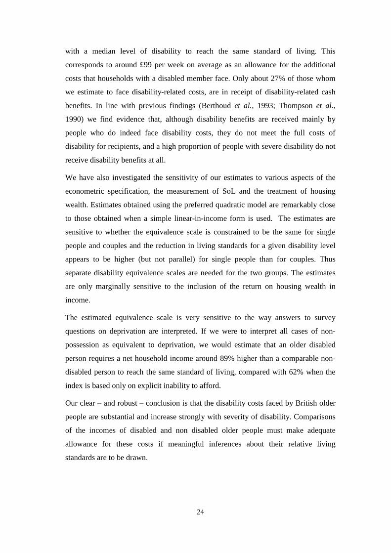
4. PARAMETER ESTIMATES AND ANALYSIS 4.1. ESTIMATES OF THE STRUCTURAL EQUATION MODEL

Estimation results for the model comprising equations (9)-(12) are presented and

discussed in Tables 4-6.7 The log-quadratic form of the SoL equation fits the data

best (see Table 7). The estimated measurement equations (9) and (10) using this form

of the SoL equation, are summarised in Tables 4 and 5. They show respectively the

factor loadings λq which capture the effect of the latent standard of living index φ on

the indicators Sq , and the factor loadings μk associated with the disability score η. We

also report the squared correlation of each indictor with the underlying latent

construct. The factor loadings are all positive and highly significant.

Being unable to afford to replace/renew durable goods or to keep the home in a

decent state of decoration are the most sensitive indicators of the latent SoL construct

φ; the inability to afford house insurance, hobbies or leisure activities are the least

sensitive.

6 Deposit and saving account balances, stocks, bonds, certificate deposits and other savings held by the household. The information recording the amount of liquid wealth in FRS was severely affected by non-response, which we deal with by imputation based on grossing up investment income. Financial wealth is not used as a covariate in the SoL equation. 7 Estimates were computed using the robust maximum likelihood estimator of Mplus 6.11 (Muthén and Muthén, 2010).

13

Table 4 Standard of Living measurement

Factor loadings λq and squared correlations of SoL indicators with φ

Indicator(s): Factor

Loading R2

enough money to keep your home in a decent state of decoration 1.229*** 0.710

hobby or leisure activity 0.86*** 0.545

holidays away from home one week a year 1.139*** 0.677

household contents insurance 0.864*** 0.547

friends/family round for drink or meal at least once a month 0.972*** 0.604

make savings of £10 a month or more 1.001*** 0.618

two pairs of all weather shoes for each person in the HH 0.895*** 0.564

replace any worn out furniture 1.789*** 0.838

replace or repair broken electrical goods such as fridge, washing machine 1.615*** 0.809

money to spend each week on yourself, not on your family 1.08*** 0.654

Significance: * = 10%; ** = 5%; *** = 1%; R2 is the squared correlation between Sq (Can afford to do/have things or goods indicators) and φ. Estimates are obtained using the quadratic in ln(Y) model specification.

The highest correlation with the latent disability construct is found for indicators of

difficulties with mobility, lifting and dexterity, while lower correlations are found for

indicators of cognitive disability.

Table 5 Disability measurement

Factor loadings µk and squared correlations of disability indicators with η

Indicator(s): Factor

Loading R2

difficulty in mobility (moving about) 2.138*** 0.840

difficulty with lifting, carrying or moving objects 2.435*** 0.872

difficulty with manual dexterity using hands for daily tasks 1.327*** 0.669

difficulty - continence (bladder/bowel control) 0.766*** 0.402

difficulty with communication (speech, hearing or eyesight) 0.656*** 0.330

difficulty with memory/concentration/learning/understanding 0.813*** 0.431

difficulty with recognising when in physical danger 0.737*** 0.384

difficulty with your physical co-ordination 1.382*** 0.686

difficulty in other area of life 0.465*** 0.198

Significance: * = 10%; ** = 5%; *** = 1%; R2 is the squared correlation between Dk and η. Estimates in the table are obtained using the quadratic in ln(Y) model specification.

14

Results reported in Table 6 show that the conditional mean of η increases almost

linearly with age, although we allowed for non-linearity using a spline function of

age, with a single node at the median age 73 observed in the sample. The structural

estimates provide no evidence of a significant relation with gender. Indicators

measuring economic well-being are jointly significant at the 1% level: more educated

individuals experienced a low level of disability as well as those with high current

pre-disability benefit income. A negative relation between wealth and disability

emerges and this relation involves both housing wealth (captured by owner-

occupation) and financial wealth.

Table 6

Estimates of the structural parameters of the disability equation

Covariate(s): Coeff. S.E.

Spline age 73 0.033*** 0.002

Spline age 73 and over 0.033*** 0.003

Female -0.005 0.028

Post-compulsory schooling -0.036*** 0.009

(ln) pre-disability benefit income -0.114*** 0.028

Home ownership -0.299*** 0.034

(ln) financial wealth -0.029*** 0.004

Note: Significance: * = 10%; ** = 5%, *** = 1%; ¹ Cut-off set to 73, the median age in the sample. Model also includes controls for region of residence and marital status. R2=0.127. Estimates are obtained using the quadratic in ln(Y) model specification.

Estimates for the regression coefficients of the SoL equation are reported in Table 7,

using three different functional forms of f(Y): the linear-in-income (model 1); the

linear-in-log income (model 2); and the quadratic-in-log income model (model 3).

Age, level of education, home ownership, marital status and region of residence are

found to be highly significant at the 1% level and their signs, for the most part, are as

expected. A gender dummy is not significant. Here, we focus on the structural

parameters of interest in deriving the equivalence scale. The structural estimates of

the α1 and γ provide strong evidence that latent disability and current income affect

the SoL. Increased disability is associated with lower values of the SoL index, while

income is positively associated with the SoL, no matter which functional form is

used. Holding other variables constant, a 1-standard deviation increase in disability η

15

produces a reduction of 0.233 standard deviations in φ using model 1, 0.254 using

model 2 and 0.236 using model 3. The estimated income coefficients imply that a

£10 increase in weekly income increases SoL by 0.03 standard deviations in model 1

and in model 2 a 10% increase in net income produces an increase of about 0.0631

standard deviations in the SoL. In model 3, the coefficient associated with the added

square of log household income is significant at the 1%, implying a significant non-

linear relationship of income and the SoL index φ. Thus, controlling for disability

level, disability costs appear to vary with income in both absolute terms and as a

proportion of income.

At the bottom of Table 7 we report the number of free estimated regression

parameters (k), the maximized log-likelihood (L) and its correction for non normality

factor (CF), the Akaike information criterion AIC and the Bayesian Information

criterion BIC for the model comprising equations (9)-(12). According to these

measures the quadratic-in-log form (model 3) fits the data best but, as the plots in

Figure 2 show, its implications are remarkably close to those of the linear

specification.

Table 7 The standard of living equation: parameter estimates for latent disability and income

Parameter(s):

Model (1) linear in Y

Model (2) linear in ln(Y)

Model (3) quadratic in ln(Y)

Coeff. S.E. Coeff. S.E. Coeff. S.E.

𝛼1𝑆𝑇𝐷 -0.233*** 0.016 -0.254*** 0.016 -0.236*** 0.016

𝛾1𝑆𝑇𝐷 0.003*** 0.001 0.631*** 0.026 -2.61*** 0.201

𝛾2𝑆𝑇𝐷 0.307*** 0.019

K 74 74 75

L -38718.413 -38759.401 -38694.623

CF 1.004 0.992 0.994

AIC 77584.826 77666.803 77539.247

BIC 78103.552 78185.529 78064.983

Notes: Significance: * = 10%; ** = 5%, *** = 1%. Models also include regional dummy variables and controls for socio-economic characteristics which are reported in Appendix B. R2 of model (1), (2) and (3) are 0.384; 0.334; and 0.382, respectively.

16

Figure 2 Estimated form of the Income-SoL profile

4.2. DISABILITY COSTS AND EQUIVALENCE SCALES

On the basis of the parameter estimates displayed in table 7 and after selecting the

reference level of disability D0, we can derive the relative/absolute costs of disability,

under the three models, defined as the minimal compensating amount (3). The

procedure is as follows. First, we calculate the model-based posterior prediction �̂� as

the estimate of the expectation of η conditional on all observed information for the

individual. Second, we calculate the estimate of disability cost as (4), (5) or (7)

evaluated at the point �̂�. Finally, we calculate means of these estimated costs by

decile of �̂�.8

Since we use a continuous measure of disability, the definition of D0 is less

straightforward than when using a dichotomous indicator. We can think of D0 as a

reference level of disability above which some financial compensation is judged

8 Note that this is a conservative estimate, for the log-linear and (to a lesser extent) the log-quadratic model. Because of the convexity of the exp(.) function in (5) and (7), the true average cost will be understated: to a degree that depends on the posterior variance of η.

0

0.5

1

1.5

2

2.5

£100 £300 £500 £700 £900

SoL

Income per week

Linear

Log-linear

Log-quadratic

17

appropriate, but how should this reference level be chosen? Table 8 reports the

prevalence of reported difficulties by decile of �̂�. As noted in section 4, about 53% of

the sample reported some disability. All individuals who fall in the highest four

deciles of �̂� reported at least one disability, most having a difficulty with mobility,

lifting, carrying or moving objects. The mean number of reported disabilities

increases non-linearly with position in the latent disability distribution. It is clear

from Table 8 that there is a definite discontinuity at the median and, as a

consequence, we adopt the median level of �̂� (D0 = 0.972) as our reference level.

Figure 3 shows the empirical kernel distribution of the predicted disability index �̂�

from the log-quadratic model.

Table 8 Self-reported difficulties by decile of �̂�

% of those who reported

Number of difficulties reported Decile of �̂� any difficulties

difficulties with mobility, lifting, carrying or moving objects

1 0.0% 0.0% 0.00

2 0.0% 0.0% 0.00

3 0.0% 0.0% 0.00

4 0.2% 0.0% 0.00

5 5.5% 0.0% 0.06

6 63.2% 2.3% 0.67

7 100.0% 91.8% 1.22

8 100.0% 98.4% 2.22

9 100.0% 100.0% 3.03

10 100.0% 100.0% 4.97

Mean 46.9% 39.2% 1.22

Notes: Statistics computed over a sample of 8,183 FRS 2007-8 respondents.

18

Figure 3 Kernel Density Estimator of η

Notes: vertical line represents the reference level of disability (D0).

Income and receipt of disability benefits by decile of latent disability are displayed in

Table 9. Average weekly post-disability benefit household income (Y) is reported

per-capita and without adjustment for household composition. The association

between disability and socio-economic status is widely recognized (see for instance

Cutler et al., 2011 and Goldman, 2001 for a review) although the extent to which this

association reflects causality is still in debate (Conti et al., 2010). Similarly we find

that there is a strong association between disability and per-capita income which

declines monotonically until the fifth decile of η and is almost flat afterwards. Thus

poor health and low income are strongly associated even if the measure of income

used, as here, includes the disability benefit that individuals receive. The last 3

columns of Table 9 show the percentage of individuals in the sample in receipt of

any disability benefit by decile of latent disability, the proportions of those recipients

who are in each disability decile and the average amount of disability benefits

received by individuals in each disability decile. The proportion of individuals in the

sample who receive these benefits ranges from under 2% in the lowest disability

decile to 50% in the top decile. Overall, amongst those in the upper half of the

disability distribution the percentage is 27%. Although current disability benefits

appear well targeted on disabled people, a significant proportion of those who face

severe disability do not receive disability benefits. Non take-up of disability benefits

19

among disabled people has been noted elsewhere (Pudney, 2010, Currie and

Madrian, 1999) and the receipt of disability benefit may often be delayed by several

years after disability onset (Zantomio, 2010).

Table 9

Mean income and receipt of disability benefits by deciles of latent disability

Decile of �̂�

Mean Ya

£s pw, 2007 prices % of individuals receiving disability benefits

% of individual disability benefit recipients in each disability decile

Average amount of disability benefitb

received £s pw, 2007

prices

Per capita Unadjusted

for household composition

1 263.90 442.90 1.8 1.2 1.20

2 206.00 353.10 3.2 2.0 1.90

3 187.40 309.10 3.6 2.3 2.30

4 162.80 257.70 5.0 3.2 2.70

5 141.30 203.80 6.9 4.4 4.00

6 148.70 221.50 10.3 6.6 6.30

7 172.20 264.10 15.5 10.0 10.00

8 175.50 263.80 24.1 15.4 15.70

9 174.10 255.50 35.6 22.8 23.50

10 181.70 264.10 50.1 32.1 37.80

Mean for deciles 6 to 10 170.40 253.80 27.1 86.9 18.60

Notes: Statistics computed over a sample of 8,183 FRS 2007-8 respondents. All monetary values are rounded to the nearest 10p. a. Household income including disability benefit. b. Measured at the individual level.

Estimated costs of disability are presented in Table 10. There are 260 cases (out of

8,183 in the estimation sample) where the condition 𝐶 ≤ 𝛾12/4𝛾2 in equation (8) is

violated. All have a combination of low income (mean £88 compared to £290 for the

full sample) and low estimated latent disability (mean 0.65 compared to 1.40). In the

calculations reported below, we set their disability costs to zero; the alternative

procedure of dropping cases with very low income and disability leads to virtually

identical estimates.

Average estimated disability costs (∆) and the equivalence scale (σ) are displayed in

Table 10 by deciles of �̂� (above the median) for each of the three model variants9. On

9 Appendix A reports equivalence scales and disability costs among disabled people by deciles of household income.

20

average, a person in the upper 50% of the disability distribution requires an

additional £90 to reach the same standard of living as a comparable person at the

median level of disability, according the linear model. Average disability costs are

about £17 per week in the sixth decile of the disability distribution, rising to £164 in

the top decile. For the log-linear specification the estimated disability costs are

higher (about £154 per week for those in the upper 50% of disability) and they

increase more sharply with disability. The log-quadratic model generates estimates

which are much closer to those of the linear model, but with slightly higher values in

the upper tail of the disability distribution. The estimated average cost of disability

among the upper 50% of disabled people is about £99 per week; in the top decile of

disability it is £180.

The most important observation on the estimates of the equivalence scale (σ) is that σ

increases with disability10. If we define a disabled person as someone with a

disability in the top half of the disability distribution, an older disabled person

requires, on average, an increase of about 55% of net weekly pre-disability

household income (Y0) to reach the same standard of living as a comparable non-

disabled person, according to the linear model. Average disability costs are about

11% of Y0 in the sixth decile of the disability distribution, rising to 106% in the top

decile. For the log-linear specification, estimated disability costs are about 65%

higher on average in the disabled population and increase more sharply with

disability. The log-quadratic model generates estimates which are much closer to

those of the log-linear model, but with slightly lower values in the upper tail of the

disability distribution. The average extra cost of disability is about 62% of the net

weekly pre-disability household income.

10 By construction, σ obtained using model 1 and 2 is lower than 1 for those individuals who fall below the median level of disability [𝑔(𝐷) < 𝑔(𝐷0)] and increases afterwards. However, nothing prevents the equivalence scale derived from model 3 for some people with disability level below D0 from being greater than 1. That is because the base dependent equivalence scale we derived from specification 3 while increases with level of disability, it is a decreasing function of income. In practice this occurs for only 1.07% of the sample.

21

Table 10

Estimated costs of disability and average equivalence scale by deciles of latent

disability

Decile of �̂� Model (1) linear in Y

Model (2) linear in ln(Y)

Model (3) quadratic in ln(Y)

∆ £s pw, 2007 prices σ ∆

£s pw, 2007 prices σ ∆ £s pw, 2007 prices σ

6 17.40 1.11 23.10 1.10 22.10 1.21

7 62.00 1.35 95.10 1.38 67.80 1.40

8 91.00 1.50 149.60 1.60 98.00 1.54

9 116.30 1.72 193.10 1.83 126.10 1.78

10 163.70 2.06 307.50 2.36 179.90 2.17 Mean for deciles 6 to

10 90.0 1.55 153.60 1.65 98.70 1.62

Notes: Estimates of ∆ are unadjusted for household composition. All monetary values are rounded to the nearest 10p. Reference disability level for computing ∆ and σ is the median.

5. SENSITIVITY ANALYSIS

In this section we discuss the sensitivity of our results to (i) the assumption that the

costs of disability and the equivalence scale are independent of household

composition, (ii) the income definition, and (iii) the construction of the SoL measure.

Demographic invariance The three models of the previous section imply

invariance of the equivalence scale to household size and structure. This has the

advantage that a benefit system with the same property does not create incentives for

potential claimants to change their household type to increase their level of

entitlement (Pendakur, 1999). We test whether estimates of the best-fitting quadratic

model are sensitive to the assumption of demographic invariance by using a two-

group analysis where we allow the parameters of the SoL equations (9) and (11) to

differ for respondents from single-person and two-person households. In contrasting

this with the unrestricted model, the Akaike information criterion suggests that the

unrestricted model provides a slightly better balance of model fit and parsimony. In

contrast, a Satorra-Bentler test (Muthén and Muthén, 2005) gives a χ2(27)-statistic of

70.85 (p=0.000) in favour of the restricted one. Panel (1) in table 11 shows the

equivalence scale and the extra cost of disability computed for single people and

couples, by disability index η. It should be noticed however, that about 58% of single

people, compared with 44% of couples, belong to the top four deciles of �̂�. Thus

22

single people (mainly widows) on average experience higher disability levels than

people in couples (see also Zaidi and Burchardt, 2005). On the other hand, household

income (not adjusted for household composition) of people in couples is generally

higher than for single people. So that the reduction in the living standard caused by a

given disability level is higher (lower) in relative (absolute) terms for single people

than couples.

Housing wealth A further sensitivity analysis makes some allowance for

housing wealth. We re-estimate equations (9)-(12) adding to the income variables in

equations (11) and (12) an annual return from the (estimated) house wealth of 2%

and 4%, respectively11. This increases the household income measure only for the

76% of people who are owner occupiers. Estimates of equivalence scales and the

extra costs of disability using a 2% and 4% return on housing wealth are remarkably

close to the base case and are reported in panel (2) of Table 11.

Interpretation of SoL indicators A final sensitivity test sets the indicators S

equal to 0 even in cases where respondents replied “We/I do not want/need this” to

the deprivation question (see section 2). This produces a lower coefficient for η (-

0.272) a higher 𝛾1𝑆𝑇𝐷 (-1.793) and a lower 𝛾2𝑆𝑇𝐷 (0.217), yielding an estimate of the

extra cost of disability among disabled people of about 89% of their household

income. Results are shown in panel (4) of Table 11.

11 Estimates of housing wealth are derived by estimating an interval regression using recorded Council Tax band information and a set of controlling characteristics available in the FRS. Council Tax is a local property tax for which all domestic properties have been valued and the value placed in a band. This regression gives us a vector of estimated coefficients with we use to derive homeowners’ expected housing wealth conditional on being in the respondent council tax band, evaluated at the time when their properties were last valued (1991 for England and Scotland and 2005 in Wales). Finally, observed regional changes in house prices between then and 2007 are applied to yield estimated housing wealth in 2007 prices. Return on housings wealth is then computed at a weekly basis (dividing the assumed annual return by 52).

23

Table 11

Sensitivity Analysis: mean costs of disability and equivalence scale by deciles of η

Decile of �̂�

(1) (2) Returns from Housing wealth (3)

Couples Singles 2% 4%

SoL indicator = 0 if does not want/ have / or cannot afford to, 1

otherwise (N=4,752) (N=3,438)

∆ £s pw, 2007

prices σ

∆ £s pw, 2007

prices σ

∆ £s pw, 2007

prices σ

∆ £s pw, 2007

prices σ

∆ £s pw, 2007

prices σ

6 23.60 1.11 14.70 1.15 21.40 1.20 21.70 1.20 29.90 1.23 7 74.00 1.31 55.40 1.42 66.30 1.39 67.30 1.40 100.70 1.56 8 108.20 1.43 80.60 1.57 96.10 1.52 97.40 1.53 148.90 1.78 9 139.00 1.55 102.40 1.82 123.50 1.76 125.20 1.77 192.20 2.13

10 197.10 1.82 147.40 2.25 176.30 2.14 178.90 2.15 281.30 2.74 Mean

for deciles 6 to 10

107.60 1.44 80.60 1.65 96.70 1.60 98.10 1.61 150.50 1.89

Notes: Estimates of ∆ are unadjusted for household composition. All monetary values are rounded to the nearest 10p.

6. DISCUSSION AND CONCLUSIONS

In this paper, we have applied the standard of living approach to estimate the cost of

disability among older people in Great Britain and extended previous research by

developing a two-latent factor structural model to estimate equivalence scales for

disability. Disability is treated as a latent construct which is measured imperfectly by

a vector of survey indicators and is influenced by observed socio-economic

characteristics. Ten indicators of deprivation are used as observable counterparts of

the latent continuous index of SoL, which varies in relation to household income and

disability. Our approach allows us to construct a base-independent equivalence scale

which takes account of the severity of disability. The restrictions on preferences

imposed by the assumption of a base-independent equivalence scale for disability are

not supported by our data. This implies that the extra income that disabled people on

higher incomes need to be as well off as their non-disabled counterparts is lower than

the equivalent sum needed by disabled people on lower incomes. Our application is

the first, in our knowledge, to derive an equivalence scale for disability using a log-

quadratic function on income of the kind that has been used in Engel curve studies.

The results show that the extra costs of disability are substantial, and rise with

severity. Using the 2007/8 wave of the FRS we estimate that an older disabled

person, defined as someone above the median level of disability for all older people,

requires a net household income around 62% higher than that of a comparable person

24

with a median level of disability to reach the same standard of living. This

corresponds to around £99 per week on average as an allowance for the additional

costs that households with a disabled member face. Only about 27% of those whom

we estimate to face disability-related costs, are in receipt of disability-related cash

benefits. In line with previous findings (Berthoud et al., 1993; Thompson et al.,

1990) we find evidence that, although disability benefits are received mainly by

people who do indeed face disability costs, they do not meet the full costs of

disability for recipients, and a high proportion of people with severe disability do not

receive disability benefits at all.

We have also investigated the sensitivity of our estimates to various aspects of the

econometric specification, the measurement of SoL and the treatment of housing

wealth. Estimates obtained using the preferred quadratic model are remarkably close

to those obtained when a simple linear-in-income form is used. The estimates are

sensitive to whether the equivalence scale is constrained to be the same for single

people and couples and the reduction in living standards for a given disability level

appears to be higher (but not parallel) for single people than for couples. Thus

separate disability equivalence scales are needed for the two groups. The estimates

are only marginally sensitive to the inclusion of the return on housing wealth in

income.

The estimated equivalence scale is very sensitive to the way answers to survey

questions on deprivation are interpreted. If we were to interpret all cases of non-

possession as equivalent to deprivation, we would estimate that an older disabled

person requires a net household income around 89% higher than a comparable non-

disabled person to reach the same standard of living, compared with 62% when the

index is based only on explicit inability to afford.

Our clear – and robust – conclusion is that the disability costs faced by British older

people are substantial and increase strongly with severity of disability. Comparisons

of the incomes of disabled and non disabled older people must make adequate

allowance for these costs if meaningful inferences about their relative living

standards are to be drawn.

25

REFERENCES Adams, P., Hurd, M. D., McFadden, D., Merrill, A., and Ribeiro, T. (2003). Healthy,

wealthy, and wise? Tests for direct causal paths between health and socioeconomic status. Journal of Econometrics,112(1), 3-56.

Banks, J., Blundell, R., and Lewbel, A. (1997). Quadratic Engel curves and consumer demand. The Review of Economics and Statistics, 79(4), 527-539.

Berthoud, R, Lakey, J., and McKay, S. (1993). The Economic Problems of Disabled People. London: Policy Studies Institute.

Berthoud, Richard. (1991). Meeting the costs of disability. In G. Dalley (Ed.), Disability and Social Policy. London: Policy Studies Institute.

Berthoud, Richard, Blekesaune, M., and Hancock, R. (2009). Ageing, income and living standards: evidence from the British Household Panel Survey. Ageing and Society, 29(07), 1105.

Burchardt, Tania. (2004). Capabilities and disability: the capabilities framework and the social model of disability. Disability and Society, 19(7), 735-751.

Conti, G., Heckman, J., and Urzua, S. (2010). The education-health gradient American Economic Review, 100 (2), pp. 234-38.

Coulter, F. A. E., Cowell, F. A., and Jenkins, S. P. (1992). Differences in needs and assessment of income distributions. Bulletin of Economic Research, 44(2), 77-124.

Cullinan, J, Gannon, B, and Lyons, S. (2011). Estimating the extra cost of living for people with disabilities. Health Economics, 20 (5), 582-599.

Currie, J., and Madrian, B. C. (1999). Health, health insurance and the labor market. In O. Ashenfelter and D. Card (Eds.), Handbook of Labor Economics vol. 3C (pp. 3309-3416). New York: Elsevier Science.

Cutler, D. M., Lleras-Muney, A., and Vogl, T. (2011). Socioeconomic status and health: dimensions and mechanisms. In S. Glied, P.C. Smith (Ed.), Oxford Handbook of Health Economics, Oxford: Oxford University Press

Deaton, A., and Paxson, C. (1998). Economies of scale, household size, and the demand for food. Journal of Political Economy, 106(5), 897-930.

Department for Work and Pensions. (2009). Households Below Average Income 1994/95-2007/2008. London, The Stationery Office.

Department for Work and Pensions. (2009). Family Resources Survey, 2007–8. London, The Stationery Office.

Doessel, D. P., and Whiteford, H. (2004). Applying concepts from Mill and Sen to the standard of living for disabled people. Mimeo. Brisbane: Queensland Centre for Mental Health Research, University of Queensland, Australia, 1-27. Retrieved from http://www.ecosoc.org.au/files/File/TAS/ACE07/presentations (pdf)/Doessel.pdf.

Feinstein, A. R., Josephy, B. R., and Wells, C. K. (1986). Scientific and clinical problems in indexes of functional disability. Annals of Internal Medicine, 105(3), 413-420.

Goldman, N. (2001). Inequalities in health: disentangling the underlying mechanisms. In A. Weinstein, M., Hermalin (Ed.), Strengthening the Dialogue between Epidemiology and Demography. Annals of the New York Academy of Sciences.

26

Gordon, D., Adelman, L., Ashworth, K., Bradshaw, J., Levitas, R., Middleton, S., Pantazis, C., Patsios, D., Payne, S., Townsend, P. and Williams, J. (2000). Poverty and Social Exclusion in Britain. York: Joseph Rowntree Foundation.

Hancock, R., and Pudney, S. (2010). The distributional impact of reforms to disability benefits for older people in the UK. University of Essex: ISER Working Paper no. WP2010-35.

Hartigan, I. (2007). A comparative review of the Katz ADL and the Barthel Index in assessing the activities of daily living of older people. International Journal of Older People Nursing, 2(3), 204-212.

Jones, A., and O’Donnell, O. (1995). Equivalence scales and the costs of disability. Journal of Public Economics, 56(2), 273-289.

Kasparova, D., Marsh, A., and Wilkinson, D. (2007). The take-up rate of Disability Living Allowance and Attendance Allowance : Feasibility study. London: Department for Work and Pensions, Research Report No 442.

Katz, S., Ford, A. B., Moskowitz, R. W., Jackson, B. A., and Jaffe, M. W. (1963). Studies of illness in the aged. The Journal Of The American Medical Association, 185(12), 914-919.

Lelli, S. (2005). Using functionings to estimate equivalence scales. Review of Income and Wealth, (2), 255-285.

Lewbel, A. (1997). Consumer demand systems and household equivalence scales. Handbook of Applied Econometrics, 2, 167-201. Oxford: Blackwell.

Mahoney, F. I., and Barthel, D. W. (1965). Functional evaluation: the Barthel Index. Maryland State Medical Journal, 14(2), 61-65. Martin, J., and White, A. (1988). The financial circumstances of disabled adults living in private households. London: HMSO.

Mckay, S. (2004). Poverty or preference: What do “Consensual Deprivation Indicators” really measure? Fiscal Studies, 25(2), 201-223.

Mckay, S. (2008). Measuring material deprivation among older people : Methodological study to revise the Family Resources Survey questions. London: Department for Work and Pensions, Working Paper No 54.

Morciano, M., Zantomio, F., Hancock, R., and Pudney, S. (2010). Disability status and older people’s receipt of disability benefit in British population surveys : a multi-survey latent variable structural equation approach. Paper presented at the Winter Health Economists' Study Group (HESG) meeting, London.

Muellbauer, J. (1979). McClements on equivalence scales for children. Journal of Public Economics, 12, 221-231.

Muthén, L. K., and Muthén, B. O. (2005). Chi-square difference testing using the S-B scaled chi-square. Note on Mplus website, www.statmodel.com.

Muthén, L. K., and Muthén, B. O. (2010). Mplus User’s Guide. Sixth Edition. Los Angeles: Muthén and Muthén. Retrieved from http://www.statmodel.com.

Nelson, J. A. (1993). Household equivalence scales: Theory versus policy? Journal of Labor Economics, 11(3), 471.

Pendakur, K. (1999). Semiparametric estimates and tests of base-independent equivalence scales. Journal of Econometrics, 88(1), 1-40.

Pollak, R. A., and Wales, T. J. (1979). Welfare comparisons and equivalence scales. The American Economic Review, 69(2), 216–221.

27

Pudney, S. (2010). Disability benefits for older people: How does the UK Attendance Allowance system really work ? University of Essex, ISER Working Paper no. 2010-02.

Saunders, P. (2007). The costs of disability and the incidence of poverty. Australian Journal of Social Issues, 42(4), 461-480.

Smith, N., Middleton, S., Ashton-Brooks, K., Cox, L. and Dobson, B. (2004) Disabled people’s costs of living: more than you would think York: Joseph Rowntree Foundation

Stapleton, D., Protik, A., and Stone, C. (2008). Review of international evidence on the cost of disability. Department of Work and Pensions research report 542. Retrieved from http://statistics.dwp.gov.uk/asd/asd5/rports2007-2008/rrep542.pdf

Stewart, M. B. (2009). The estimation of pensioner equivalence scales using subjective data. Review of Income and Wealth 55(4), 907-929.

Thompson, P, Lavery, M, and Curtice, J (1990) Short-changed by Disability London: Disability Income Group

Zaidi, A., and Burchardt, T. (2005). Comparing incomes when needs differ: Equivalization for the extra costs of disability in the UK. Review of Income and Wealth, 51(1), 89-114.

Zantomio, F. (2010). Older people’s participation in disability benefits: targeting, timing and financial wellbeing. University of Essex, ISER Working Paper no. WP 2010-23.

28

APPENDIX A:

EQUIVALENCE SCALE AND DISABILITY COSTS AMONG PEOPLE IN THE UPPER 50% OF THE DISABILITY DISTRIBUTION BY DECILES OF PER CAPITA Y

Decile of per capita pre-disability benefit

incomea (% of disabled peopleb

in each decile)

mean Yc

£s pw, 2007 prices Model (1) linear in Y

Model (2) linear in ln(Y)

Model (3) quadratic in ln(Y)

Per-capita

Unadjusted for

household composition

∆ £s pw, 2007 prices

σ ∆

£s pw, 2007 prices

σ ∆

£s pw, 2007 prices

σ

1 (60.1%) 95.10 141.50 95.60 2.16 81.50 1.72 115.60 2.65

2 (59.6%) 109.40 180.20 88.10 1.63 106.10 1.64 89.70 1.65

3 (56.7%) 127.60 204.50 89.80 1.56 120.70 1.65 90.90 1.57

4 (63.8%) 136.20 186.60 87.30 1.58 111.30 1.63 87.90 1.57

5 (55.0%) 149.30 211.40 89.20 1.51 133.20 1.65 91.00 1.51

6 (52.1%) 167.90 249.50 92.70 1.47 155.00 1.68 96.20 1.47

7 (46.2%) 192.90 287.40 89.90 1.39 167.40 1.65 95.40 1.41

8 (42.7%) 226.40 344.70 88.80 1.31 205.80 1.63 100.80 1.34

9 (33.2%) 270.00 403.50 90.10 1.27 246.90 1.64 108.60 1.31

10 (30.4%) 412.10 594.90 88.10 1.17 377.80 1.63 130.20 1.23

Overall mean (50.0%) 170.40 253.80 90.00 1.55 153.60 1.65 98.70 1.62

Notes: a. Deciles computed over the pre-disability benefits income distribution of the whole population which includes non-disabled people. b. Disabled people defined as those in the upper 50% of the distribution of disability c. Household income including disability benefit. ∆s are unadjusted for household composition. Monetary values are rounded to the nearest 10p.

29

APPENDIX B: PARAMETER ESTIMATES FROM THE STANDARD OF LIVING EQUATION IN THE

THREE VARIANTS

Covariate(s):

Model (1) Linear in Y

Model (2) Linear in ln(Y)

Model (3) Quadratic in ln(Y)

Coeff. S.E. Coeff. S.E. Coeff. S.E.

η -0.277*** 0.020 -0.29*** 0.020 -0.281*** 0.020

(in s.d. units) -0.233*** 0.016 -0.254*** 0.016 -0.236*** 0.016

linear in Y 0.003*** 0.000

(in s.d. units) 0.003*** 0.000

linear in ln(Y)

0.79*** 0.036 -3.424*** 0.272

(in s.d. units)

0.645*** 0.026 -2.691*** 0.201

quadratic in ln(Y)

0.4*** 0.027

(in s.d. units)

0.315*** 0.019

Female -0.005 0.033 0.002 0.033 -0.004 0.033

(in s.d. units) -0.004 0.026 0.002 0.027 -0.003 0.026

Spline age 73a 0.034*** 0.004 0.03*** 0.004 0.034*** 0.005

(in s.d. units) 0.026*** 0.003 0.025*** 0.004 0.027*** 0.004

Spline age 73plusa 0.037*** 0.004 0.038*** 0.004 0.037*** 0.004

(in s.d. units) 0.029*** 0.003 0.031*** 0.003 0.029*** 0.003

Post-compulsory schooling 0.043*** 0.012 0.062*** 0.011 0.041*** 0.012

(in s.d. units) 0.034*** 0.009 0.051*** 0.009 0.032*** 0.009

Home owner 0.497*** 0.037 0.481*** 0.037 0.486*** 0.037

(in s.d. units) 0.39*** 0.030 0.393*** 0.030 0.382*** 0.029

Married/cohabiting -0.195*** 0.041 -0.222*** 0.039 -0.238*** 0.040

(in s.d. units) -0.153*** 0.031 -0.181*** 0.032 -0.187*** 0.031

Notes: Significance: * = 10%; ** = 5%, *** = 1%. a. Cut-off set to 73, the median age in the sample. All models also contain controls for region of residence.