HAL Id: hal-01653074https://hal.archives-ouvertes.fr/hal-01653074

Preprint submitted on 1 Dec 2017

HAL is a multi-disciplinary open accessarchive for the deposit and dissemination of sci-entific research documents, whether they are pub-lished or not. The documents may come fromteaching and research institutions in France orabroad, or from public or private research centers.

L’archive ouverte pluridisciplinaire HAL, estdestinée au dépôt et à la diffusion de documentsscientifiques de niveau recherche, publiés ou non,émanant des établissements d’enseignement et derecherche français ou étrangers, des laboratoirespublics ou privés.

Distributed under a Creative Commons Attribution - NonCommercial - NoDerivatives| 4.0International License

Working fluid selection general method and sensitivityanalysis of an Organic Rankine Cycle (ORC): application

to Ocean Thermal Energy Conversion (OTEC)Alexandre Dijoux, Frantz Sinama, Olivier Marc, Bertrand Clauzade, Jean

Castaing-Lasvignottes

To cite this version:Alexandre Dijoux, Frantz Sinama, Olivier Marc, Bertrand Clauzade, Jean Castaing-Lasvignottes.Working fluid selection general method and sensitivity analysis of an Organic Rankine Cycle (ORC):application to Ocean Thermal Energy Conversion (OTEC). 2017. �hal-01653074�

1

Working fluid selection general method and sensitivity analysis of an 1

Organic Rankine Cycle (ORC): application to Ocean Thermal Energy 2

Conversion (OTEC) 3

Alexandre Dijoux1, 2 *, Frantz Sinama1, Olivier Marc1, Bertrand Clauzade2, Jean-Castaing 4

Lasvignottes1 5

1 Laboratory of Physical and Mathematical Engineering for Energy and Environment, 40 6

Avenue de Soweto, 97410 Saint Pierre, Reunion Island, France. 7 2 NAVAL Energies, Centre Indret, La Montagne, France. 8

* Corresponding Author: Mail: alexandre.dijoux@univ-reunion.fr 9

Tel: +33 650 69 04 85 10

Highlights 11

Development of a general model for the choice of the working fluid using Entropic 12

Mean Temperature Difference. 13

Comparison of 26 working fluids over 107 according to four criteria: technicity of the 14

installation, security, environmental impacts and thermodynamic performances. 15

Good candidates for an application to OTEC: NH3, R507a and R1234yf 16

Parametric sensitivity analysis of the model. 17

Keywords 18

Ocean Thermal Energy Conversion (OTEC); Entropic Mean Temperature Difference (EMTD); 19

Organic Rankine cycle (ORC); parametric sensitivity analysis. 20

Abstract 21

A general model of an ORC (Organic Rankine Cycle) that is applicable to various technologies 22

of heat exchangers has been carried out. It has been done considering the entropic mean 23

temperature difference between the heat source and the working fluid as a parameter for heat 24

exchangers. This model allows to compare pure fluids and mixtures in similar operating 25

conditions. Simulations were conducted in the case of OTEC (Ocean Thermal Energy 26

Conversion), for which the inputs are based on experimental measurements on an onshore 27

prototype in Reunion Island. 26 fluids have been compared, considering thermodynamic 28

performances (thermal efficiency and volumic work), technicity, security and environmental 29

impacts. In the end, NH3, R507a and R1234yf appears to be the most suitable ones. In order to 30

have a better understanding of the model and to determine its validity in the whole domain of 31

variation of the parameters for OTEC, a parametric sensitivity analysis has been carried out by 32

ANOVA (ANalysis Of VAriance) associated to polynomial chaos expansion method. The most 33

sensible parameters are heat source temperature, heat exchangers entropic mean temperature 34

difference and turbine isentropic efficiency. The ranking given for the fluids is still valid in the 35

whole range of the parameters for OTEC. 36

37

2

1. Introduction 1

Ocean Thermal Energy Conversion (OTEC) is a great opportunity in the tropical belt to produce 2

non-fluctuant and environmentally friendly power [1]. The temperature difference between hot 3

surface and cold deep seawater is exploited through a power cycle in order to produce electricity 4

[2]. The temperature difference between hot and cold heat sources is very small compared to 5

conventional Rankine cycles, or even compared with other applications working at low 6

temperature, such as solar, geothermal or waste heat recovery [3]. 7

Various approaches are used in order to increase the very low performance of an ORC (Organic 8

Rankine Cycle): 9

modifying the cycle structure, 10

optimizing the working conditions of the cycle, 11

choosing the most adapted working fluid for the application. 12

Considering the first point, Tchanche et al. have reviewed a lot of modified cycles (with a 13

reheater for instance), or mixtures-adapted cycle like the Kalina cycle or Uehara cycle [4]. In 14

parallel, Yoon et al. proposed an ammonia-based power cycle by using an expansion valve and 15

a cooler [5] and Yuan et al. presented a water-ammonia based power absorption cycle with two 16

ejectors [6]. They both obtained better thermal efficiency than the conventional ORC, even if 17

the Kalina and Uehara cycles also show good performances [7]–[11]. Nonetheless, the basic 18

ORC appears to be the simplest, and provides reliability, low investment costs, and easy 19

maintenance [12]. 20

Considering the choice of the working fluid, various criteria and methods have been proposed 21

to select the most suitable fluids. The main ones for a working fluid are good thermodynamic 22

performances, non-toxicity, small environmental impact, low cost, availability, and 23

compatibility with pipes and components materials. Unfortunately, it is difficult to find the 24

perfect fluid that meets all of these qualities. Lee et al. [13] compared the performances of more 25

than one hundred ozone-safe working fluids for an ORC applied to waste heat recovery. They 26

found that thermodynamic performances of the fluids are correlated with their physical 27

properties, such as normal boiling point, critical pressure and molecular weight. Stijepovic et 28

al. [14] also carried out a theoretical study to evaluate the effect of physical properties of 29

workings fluids on thermal and exergetic efficiency and the ratio of heat exchangers area and 30

net power output. Saleh et al. [15] conducted simulations to compare the thermal efficiency and 31

volume flow rates of various working fluids for different types of cycle. Wang et al. [16] 32

provided a theoretical analysis of net power output and heat exchangers surface for a Waste 33

Heat Recovery (WHR) system. They found that fluids with low Jacob number performed better. 34

They also found in another study [17] that the choice of the working fluid for WHR has a small 35

impact on optimal performances of the cycle, and that the evaporator is the most important 36

component in exergy losses. However, they only consider pure fluids. The use of mixtures as 37

working fluid has also been discussed [18], [19]. It is established that, in theory, the behavior 38

of mixtures during phase change allows reducing the mean temperature difference between 39

working fluid and source in heat exchangers, but the performance is not always better than pure 40

fluids in practice. Some authors realized a complete cost study by using correlations for several 41

3

components [17], [20]–[22]. This means that they should choose a precise technology of heat 1

exchangers and expander. Zhang et al. [23] proposed a method using the Hass Diagram 2

Technique to compare working fluids with thermodynamic, security and environment 3

considerations. However, no simulation was conducted to evaluate thermodynamic behavior of 4

each fluid in a particular cycle. 5

The selection of the best fluids is also often related with the optimization of working conditions 6

parameters of the cycle, like the evaporation and condensation temperature : each fluid is thus 7

compared with his own optimized parameter [16], [24], [25]. He et al. [26] carried out an 8

analytical study in order to evaluate the optimized evaporation temperature with net power 9

output as the objective function and compared the optimal net power output for several fluids. 10

In that case, the objective function is decisive, as it influences the value of optimal parameters. 11

Therefore, some efforts have been made to conduct multi-objective optimization [27], [28]. 12

Moreover, in the case of OTEC, which is very particular due to the weak temperature difference 13

between heat sources, the literature about the choice of the working fluid is relatively poor. Sun 14

et al. [29] provided an analytical method to optimize the performance of an OTEC power plant 15

considering two working fluids, R134a and ammonia. Yang et al. [30] conducted an 16

optimization of evaporation and condensation temperature and a comparison of five pure 17

working fluids considering an OTEC power plant with shell-and-tube heat exchangers. Yoon 18

et al. [31] compared the influence of various working fluids on the thermal efficiency of an 19

OTEC power plant, but they didn’t take into account net power output or volume flow rates. 20

Iqbal et al. [32] analyzed the influence of mixtures on the performances of an OTEC system, 21

but they compared only one of them with one pure fluid (propane). Hung et al. [33] carried out 22

a comparison of eleven working fluids for solar and OTEC heat sources based on a study of 23

physical properties of the fluids. They found that isentropic fluids performed generally better. 24

Furthermore, some attention has been paid on increasing the temperature difference between 25

the cold and the hot sources of an OTEC system by coupling it with solar energy [34], [35] or 26

with the effluent of a nuclear power plant [36]. The problem is that the power produced is no 27

longer steady during all day and night, and nuclear power plant are often not available in tropical 28

islands, where OTEC seems undoubtedly to be a good opportunity. In fact, little attention has 29

been paid on comparing both pure and mixed working fluids for OTEC. 30

The previous short review shows that a lot of studies have been carried out for optimizing the 31

performances of an ORC, from simple approaches using ideal cycles (preselecting the fluid 32

before designing and sizing the components), to detailed energetic and economic studies and 33

simulations (where design and size of the components are fixed). These last methods require a 34

good knowledge about the technology of the system and its components, and are therefore not 35

applicable in a preliminary design phase of the system. As the choice of the working fluid occurs 36

early in the conception of an ORC, simple approaches are generally preferred. In this case, the 37

comparison of very different fluids (in particular when comparing pure fluids and mixtures) 38

remains tricky, especially when heat exchangers are not particularly described. To do so, some 39

authors introduce the pinch point [17], [25], defined by the minimal temperature difference 40

between the working fluid and the heat transfer fluid in the HEX (Heat Exchanger). However, 41

4

the location and the value of the pinch point depend on the fluid, the flow rates and the amount 1

of heat exchanged and are sometimes difficult to determine and require a deep knowledge of 2

the HEX structure and applied conditions. Other authors consider the temperature difference 3

between the outlet of the working fluid and the inlet of the heat source [5], [6], [37]. This method 4

is interesting when comparing pure fluids, because the phase change temperature is constant. 5

In the case of zeotropic mixtures, temperature is no longer constant during evaporation and 6

condensation and this behavior allows to reduce the mean temperature difference between the 7

working fluid and the heat source [18]. However, the temperature variation of the mixture does 8

not necessarily have the same profile as the heat source. Hence, one or more pinch points can 9

be observed [38]. So, when comparing zeotropic mixtures with pure fluids, this method 10

becomes disadvantageous. 11

To overcome these drawbacks and provide a general method to compare working fluids in 12

similar conditions with a reduce number of hypothesis, the entropic mean temperature 13

difference is introduced in this study as a parameter for heat exchangers description. In the end, 14

a general method for working fluid comparison is given, considering four criteria: technicity, 15

thermodynamic performances, security and environment. This method is implemented for an 16

OTEC application, for which input parameters are issued from an experimental land-based 17

prototype in Reunion Island [39]. A parametric sensitivity analysis of the model is then carried 18

out in order to explain the model operation, and to give the validity domain of previous results. 19

2. Cycle description 20

2.1. From the ideal Carnot cycle to the real ORC 21

The most efficient cycle for converting heat into work is the Carnot cycle (Figure 2.a). 22

However, this ideal cycle is not found in practice and is replaced by the Rankine cycle (Figure 23

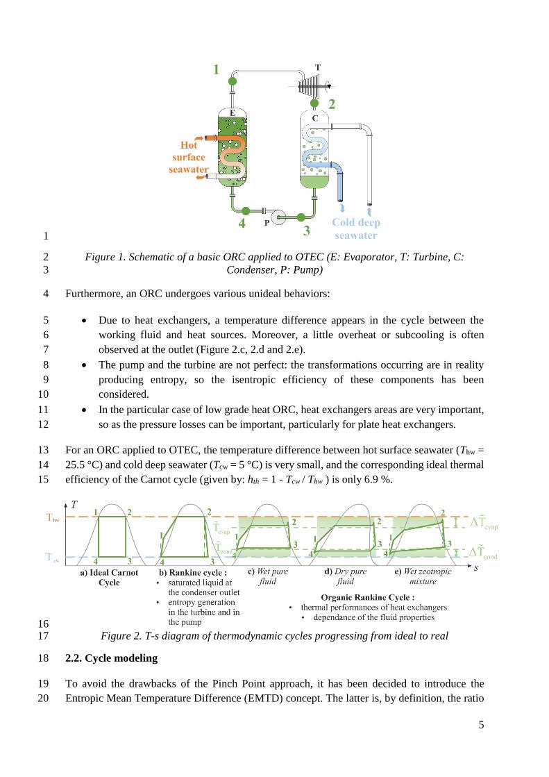
2.b). The latter is composed of four components: a pump (P), an evaporator (E), a turbine (T) 24

and a condenser (C), as shown in Figure 1. A working fluid in the liquid state (point 1) is 25

evaporated by using the heat from the hot source. The obtained vapour at high pressure (point 26

2) is expanded in the turbine producing mechanical work convertible in electricity. The vapour 27

at low pressure (point 3) is then cooled and condensed by using the cold source (point 4). A 28

pump brings back this liquid to the inlet of the evaporator (point 1). In the case of so called 29

“wet fluids” (i.e. fluids with a negative slope of their vapour saturation curve (∂T/∂s)x=1 < 0), 30

the fluid leaves the turbine in a two-phase flow, leading to droplets (Figure 2.c), whereas in the 31

case of so called “dry” or “isentropic” fluids (i.e. fluids with a positive slope or with a vertical 32

vapour saturation curve, respectively), the fluid at the output of the turbine is overheated (Figure 33

2.d and 2.e). 34

5

1

Figure 1. Schematic of a basic ORC applied to OTEC (E: Evaporator, T: Turbine, C: 2

Condenser, P: Pump) 3

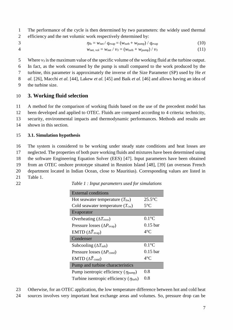
Furthermore, an ORC undergoes various unideal behaviors: 4

Due to heat exchangers, a temperature difference appears in the cycle between the 5

working fluid and heat sources. Moreover, a little overheat or subcooling is often 6

observed at the outlet (Figure 2.c, 2.d and 2.e). 7

The pump and the turbine are not perfect: the transformations occurring are in reality 8

producing entropy, so the isentropic efficiency of these components has been 9

considered. 10

In the particular case of low grade heat ORC, heat exchangers areas are very important, 11

so as the pressure losses can be important, particularly for plate heat exchangers. 12

For an ORC applied to OTEC, the temperature difference between hot surface seawater (Thw = 13

25.5 °C) and cold deep seawater (Tcw = 5 °C) is very small, and the corresponding ideal thermal 14

efficiency of the Carnot cycle (given by: hth = 1 - Tcw / Thw ) is only 6.9 %. 15

16 Figure 2. T-s diagram of thermodynamic cycles progressing from ideal to real 17

2.2. Cycle modeling 18

To avoid the drawbacks of the Pinch Point approach, it has been decided to introduce the 19

Entropic Mean Temperature Difference (EMTD) concept. The latter is, by definition, the ratio 20

6

of the enthalpy change to the entropy change, that is to say, the harmonic mean of temperature 1

weighted by heat transfer, and is given by: 2

q q hT

q s sT

(1) 3

This notion was used by Meunier et al. [40] for thermodynamic cycle analysis and by other 4

authors [41]–[43]. The EMTD is then defined by the difference between entropic mean 5

temperatures of both working and heat transfer fluids. This parameter is advantageous 6

comparing to the most used temperature difference at the output Ts since it allows the 7

comparison between pure fluids and mixtures. For the mixture, the mean temperature difference 8

is greater than that of the pure fluid due to the temperature glide. When using EMTD, fluids 9

can be compared in more similar operating conditions in terms of heat transfer, as shown in 10

Figure 3.11

12

3.a. Case when Ts is fixed 3.b. Case when �̃� is fixed

Figure 3. Typical temperature evolution profile in an evaporator throughout the heat transfer 13

progress for a pure fluid and a mixture. 14

So as to compare different kind of working fluids, it can be supposed that the entropic mean 15

temperature of the heat transfer fluid is the same for all the working fluids, taken equal to the 16

input source temperature. EMTD in the evaporator and in the condenser are then given by: 17

�̃�evap = Thw - �̃�evap (2) 18

�̃�cond = �̃�cond - Tcw (3) 19

Furthermore, considering the pump and the turbine, they are described by their respective 20

isentropic efficiency: 21

pump = (h1is – h4) / (h1 – h4) (4) 22

turb = (h3 – h2) / (h3is – h2) (5) 23

Energy balances for each component are given by: 24

Evaporator: qevap = h2 - h1 (6) 25

Turbine: wturb = h2 - h1 (7) 26

Condenser: qcond = h4 – h3 (8) 27

Pump: wpump = h1 - h4 (9) 28

7

The performance of the cycle is then determined by two parameters: the widely used thermal 1

efficiency and the net volumic work respectively determined by: 2

th = wnet / qevap = (wturb + wpump) / qevap (10) 3

wnet, vol = wnet / v3 = (wturb + wpump) / v3 (11) 4

Where v3 is the maximum value of the specific volume of the working fluid at the turbine output. 5

In fact, as the work consumed by the pump is small compared to the work produced by the 6

turbine, this parameter is approximately the inverse of the Size Parameter (SP) used by He et 7

al. [26], Macchi et al. [44], Lakew et al. [45] and Baik et al. [46] and allows having an idea of 8

the turbine size. 9

3. Working fluid selection 10

A method for the comparison of working fluids based on the use of the precedent model has 11

been developed and applied to OTEC. Fluids are compared according to 4 criteria: technicity, 12

security, environmental impacts and thermodynamic performances. Methods and results are 13

shown in this section. 14

3.1. Simulation hypothesis 15

The system is considered to be working under steady state conditions and heat losses are 16

neglected. The properties of both pure working fluids and mixtures have been determined using 17

the software Engineering Equation Solver (EES) [47]. Input parameters have been obtained 18

from an OTEC onshore prototype situated in Reunion Island [48], [39] (an overseas French 19

department located in Indian Ocean, close to Mauritius). Corresponding values are listed in 20

Table 1. 21

Table 1 : Input parameters used for simulations 22

External conditions

Hot seawater temperature (Thw) 25.5°C

Cold seawater temperature (Tcw) 5°C

Evaporator

Overheating (Tover) 0.1°C

Pressure losses (Pevap) 0.15 bar

EMTD (�̃�evap) 4°C

Condenser

Subcooling (Tsub) 0.1°C

Pressure losses (Pcond) 0.15 bar

EMTD (�̃�cond) 4°C

Pump and turbine characteristics

Pump isentropic efficiency (pump) 0.8

Turbine isentropic efficiency (turb) 0.8

Otherwise, for an OTEC application, the low temperature difference between hot and cold heat 23

sources involves very important heat exchange areas and volumes. So, pressure drop can be 24

8

observed in the working fluid side, particularly for plate HEX and have been assumed to occur 1

during the phase change of the fluid. 2

The results obtained for a list of selected working fluids is shown in Table 3. 3

3.2. Technicity 4

The first criterion used to compare working fluids in this study is the technicity represented by 5

the working pressure range and the vapour quality at the turbine outlet. Extreme pressures of 6

the cycle are calculated considering sources temperatures, while nominal pressures are 7

determined by simulated working fluid temperatures. A pressure that ranges between 1 and 24 8

bar has been considered here and provides generally easier implementation and lower cost. 9

Furthermore, the vapour quality is chosen greater than 97 % to reduce the risk of alteration of 10

the turbine by any droplets. After a first selection between a list of 107 fluids according to these 11

criteria, 26 fluids appears to be good candidates for an OTEC application. The list of selected 12

working fluids is shown in Table 3, and their technicity indicators are illustrated in Figure 4. 13

14 Figure 4 : State of the fluid at the turbine outlet and working pressure range for the 26 fluids 15

of the panel 16

It is interesting to notice that the two criteria above are correlated. Fluids with the highest 17

operating pressures are also those with the highest liquid quality at the turbine outlet. These 18

fluids are the wet fluids. Most of dry fluids have low operating pressures, but they have a high 19

overheating at the condenser inlet, which will affect cycle performances. 20

3.3. Security 21

The ASHRAE standard 34 reference [49] has been chosen as the security indicator. This latter 22

is composed of a letter that indicates the toxicity (from A for non-toxic to C for highly toxic) 23

1

8

15

22 Nominal Pressure

Extreme Pressure

Pressure level (bar)

0

1

2

3

0

1

2

3

4

5

6

Mass fraction of liquid at

the turbine outlet 1-x (%)Overheating at the turbine

outlet T-Tsat(P) ( C)

9

and a number that indicates flammability (from 1 for non-flammable to 3 for highly flammable). 1

Among the candidates, 14 fluids have the best indicator A1, as shown in Table 3. NH3 is B2L, 2

that is to say that it is toxic and slightly flammable, and R1234yf is A2L, so it is non-toxic and 3

slightly flammable. Accordingly, R1234yf shows quite good properties for safety 4

considerations, even if it isn’t A1.The indicator was not given for H2S, but it is a toxic and 5

flammable fluid. 6

3.4 Environmental considerations 7

A lot of working fluids have been forbidden in order to protect the ozone layer since the 8

Montreal protocol in 1998. Furthermore, as OTEC claim to be an environment-friendly source 9

of energy, it is important to consider the environmental impact of the working fluid. Three 10

indicators have been chosen: the global warming potential (GWP), the ozone depletion potential 11

(ODP), and the atmospheric lifetime (ALT). The GWP represents the impact on the global 12

warming in terms of temperature variation, related to that of a similar mass of CO2. The ODP 13

is the amount of destruction of the ozone layer, related to that of a similar mass of R11. The 14

ALT is the time in years necessary for a substance to turn over the global atmospheric burden. 15

Values of these three indicators are given in Figure 5. It appears that R1234yf, NH3, R600a, 16

R600 and R290 have the lowest environmental impact. 17

18 Figure 5. Value of GWP, ALT and ODP for the fluids of the panel 19

3.5. Thermodynamic performances 20

According to results given in Table 3, the ranking of the different working fluids depends 21

strongly on the selected criteria. Indeed, considering the specific work wnet, NH3 perform widely 22

better than other fluids (41.98 kJ/kg for NH3 compared to 14.98 kJ/kg for H2S in second 23

position). However, considering the thermal efficiency, the gap between different fluids is less 24

important. R143m performs better, but NH3, R236ea and SO2 give very close values of thermal 25

efficiency. Considering the net volumic work wnet, vol, H2S and R32 perform better. 26

x x

x

x x

x

x x

x x x x x

x

0.01

0.1

1

10

100

1000

10000GWP

ALT

ODP

GWP [.], ALT [years], ODP [.]

Pure fluids Azeotropic

Mixtures

Zeotropic

Mixtures

x Not Available

10

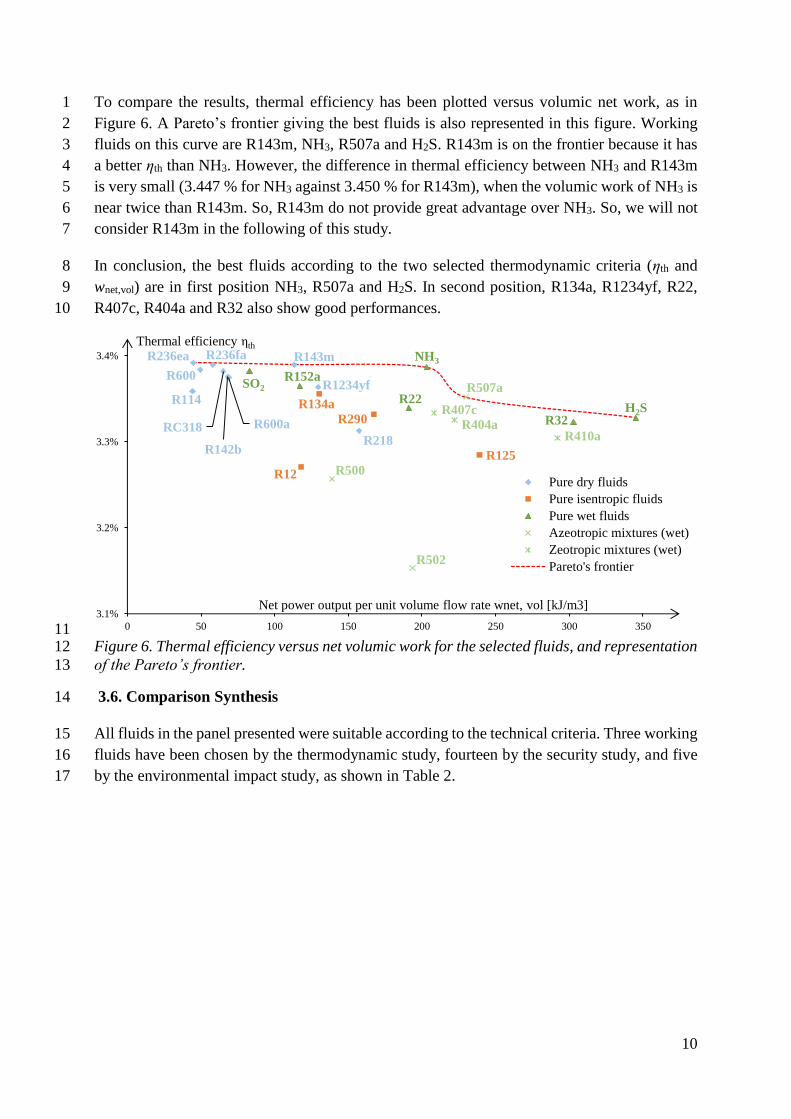
To compare the results, thermal efficiency has been plotted versus volumic net work, as in 1

Figure 6. A Pareto’s frontier giving the best fluids is also represented in this figure. Working 2

fluids on this curve are R143m, NH3, R507a and H2S. R143m is on the frontier because it has 3

a better ηth than NH3. However, the difference in thermal efficiency between NH3 and R143m 4

is very small (3.447 % for NH3 against 3.450 % for R143m), when the volumic work of NH3 is 5

near twice than R143m. So, R143m do not provide great advantage over NH3. So, we will not 6

consider R143m in the following of this study. 7

In conclusion, the best fluids according to the two selected thermodynamic criteria (ηth and 8

wnet,vol) are in first position NH3, R507a and H2S. In second position, R134a, R1234yf, R22, 9

R407c, R404a and R32 also show good performances. 10

11 Figure 6. Thermal efficiency versus net volumic work for the selected fluids, and representation 12

of the Pareto’s frontier. 13

3.6. Comparison Synthesis 14

All fluids in the panel presented were suitable according to the technical criteria. Three working 15

fluids have been chosen by the thermodynamic study, fourteen by the security study, and five 16

by the environmental impact study, as shown in Table 2. 17

R1234yf

R143m

R142b

R600

R236ea R236fa

R600a

R114

RC318R218

R134a

R12

R290

R125

SO2

NH3

R152a

H2SR22

R32

R500

R502

R507a

R410aR404a

R407c

3.1%

3.2%

3.3%

3.4%

0 50 100 150 200 250 300 350

Net power output per unit volume flow rate wnet, vol [kJ/m3]

Pure dry fluids

Pure isentropic fluids

Pure wet fluids

Azeotropic mixtures (wet)

Zeotropic mixtures (wet)

Pareto's frontier

R236ea R236fa R143m

R1234yf

Thermal efficiency ηth

NH3

H2S

SO2

11

Table 2: Best fluids from thermodynamic, security and environment point of view 1

Fluids with

better

thermodynamic

performances

Fluids with better

safety indicator

Fluids

with low

ALT,

GWP and

ODP

NH3 R507a R134a R1234yf

R507a R236fa R404a NH3

SO2 R218 R12 R600a

R114 R410a R600

R500 RC318 R290

R22 R125 R502 R407c

Table 3: Properties of selected working fluids and simulation results. The inputs for this 2

simulation are given in Table 1. 3

Type of

fluid

State at the

turbine outlet

[%]

ASHRAE wnet [kJ/kg] wnet, vol

[kJ/m3] ηth

PURE FLUIDS

R1234yf isen1 Overheated: 2.57°C A2L 5.57 129.4 3.364%

R143m isen1 Overheated: 1.37°C n.a. 2 6.76 113.2 3.390%

SO2 wet1 Diphasic: x=98.0% B1 12.74 82.9 3.383%

NH3 wet1 Diphasic: x=97.4% B2L 41.98 203.4 3.387%

R142b isen1 Overheated: 1.12°C A2 7.46 68.1 3.376%

R600 dry1 Overheated: 3.04°C A3 13.37 49.6 3.384%

R236ea dry1 Overheated: 4.40°C n.a. 2 5.89 44.7 3.392%

R152a wet1 Diphasic: x=99.3% A2 10.27 117.1 3.365%

R236fa dry1 Overheated: 4.17°C A1 5.53 57.7 3.390%

R600a dry1 Overheated: 3.07°C A3 12.28 68.8 3.375%

R114 dry1 Overheated: 4.81°C A1 4.79 44.1 3.359%

H2S wet1 Diphasic: x=97.3% n.a. 2 14.98 345.0 3.328%

R22 wet1 Diphasic: x=98.5% A1 6.73 191.0 3.340%

R134a isen1 Overheated: 0.34°C A1 6.67 130.3 3.356%

R12 wet1 Overheated: 0.08°C A1 4.97 117.9 3.271%

R32 wet1 Diphasic: x=96.6% A2 9.99 302.8 3.323%

R290 isen1 Overheated: 0.31°C A3 12.49 167.3 3.332%

RC318 dry1 Overheated: 6.38°C A1 4.07 65.2 3.382%

R125 isen1 Overheated: 0.61°C A1 4.29 239.1 3.285%

R218 dry1 Overheated: 4.98°C A1 3.08 157.2 3.313%

AZEOTROPIC MIXTURES

R500 wet1 Diphasic: x=99.7% A1 5.95 138.6 3.257%

R502 wet1 Diphasic: x=99.9% A1 4.55 193.5 3.153%

R507a wet1 Diphasic: x=99.9% A1 5.32 230.0 3.352%

ZEOTROPIC MIXTURES

R410a wet1 Diphasic: x=97.6% A1 7.01 292.0 3.305%

R404a wet1 Diphasic: x=99.9% A1 5.42 222.1 3.326%

R407c wet1 Diphasic: x=99.0% A1 7.05 208.2 3.334% 1 isentropic, wet or dry: type of the fluid depending on the slope of the saturated vapor curve 4 2 n.a.: not available 5

12

As a result, no fluid meets the three criteria at the same time. However, NH3 is a very good 1

candidate because it meets good thermodynamic performances and low environmental impact, 2

even if it is toxic. R507a is also a good candidate because it presents good thermodynamic 3

performances, non-toxicity and non-flammability, but its GWP and ALT are high. It is also 4

interesting to notice that R1234yf seems also to be a good compromise because it is in second 5

position for thermodynamic performances, it has very few environmental impacts and isn’t 6

toxic and just slightly flammable (A2L). So, in the end, three fluids appear to be the best 7

candidates for OTEC: NH3, R507a and R1234yf. This selection was made assuming operating 8

conditions and component properties to be constant. A parametric sensitivity analysis will be 9

held in the next part to study the effect of their variations. 10

4. Parametric sensitivity analysis of the thermodynamic model 11

4.1 Method 12

The parametric sensitivity analysis sets out to determine the influence of the variance of each 13

parameter of the model on the results. The most used method found in the literature is the “One 14

Factor At Time” method. This later consists in varying one parameter and keeping the others 15

constant to point out the local sensitivity of the model to this parameter. However, many 16

authors, like Saltelli and Anonni [50] or Campolongo et al. [51], consider that this method does 17

not allow a complete comprehension of the model, because it uses many shortcomings and does 18

not take into account the influence of combined effects. Thus, a global sensitivity analysis with 19

the method named ANOVA (ANalysis Of VAriance), by using the Sobol sensitivity indices 20

[52] has been chosen. We consider that every input parameter Xi is a random variable, and the 21

vector of all input parameters (X1, … , Xp) is described by its multidimensional probability 22

distribution. The model then works out the output result Y=f(X1, … , Xp), also considered as a 23

random variable whose distribution depends on that of the parameters Xi. The Sobol sensitivity 24

indices are defined by: 25

|

( ) iX i X i

i

Var E Y X

Var YS (12) 26

Where 𝑋𝑖 is the i-th input parameter and 𝑋~𝑖 represents all parameters excepted 𝑋𝑖. This 27

sensitivity index represents the reduction of the variance of the output 𝑌 if the parameter 𝑋𝑖 is 28

fixed, that is to say the percentage of the variance of 𝑌 due only to the parameter 𝑋𝑖. We can 29

also define the total sensitivity index STi as the value of the remaining variance of 𝑌 if all 30

parameters but 𝑋𝑖 are fixed: 31

|

( ) iX X i i

i

E Var Y X

VarS

YT (13) 32

Thus, 𝑆𝑇𝑖 represents the percentage of the variance of 𝑌 due to the parameter 𝑋𝑖 including its 33

interactions with other parameters. In the case of an additive model, 𝑆𝑖 = 𝑆𝑇𝑖. 34

13

In this study, all input parameters are processed to match independent random variables 1

uniformly distributed on the interval [−1,1]. Then, Polynomial Chaos Expansion, as described 2

in the work of Sudret or Crestaux et al. [53], [54] is conducted. This method is efficient when 3

the number of input parameters is lower than 20 and the function is relatively smooth. This 4

conditions are verified for this study because only 10 parameters are used and the variation of 5

outputs is continuous and regular with the variation of each parameter. 6

The model is approached by its decomposition in multidimensional polynomial series. To 7

respect the conditions of ANOVA, an orthogonal basis of Legendre polynomials is used, under 8

uniformly distributed variables in [−1,1]. The process followed is then: 9

Generation of random sets of parameters with respect to the given distribution 10

Computation of the model results for each set of parameter 11

Determination of the coefficients 𝑎𝑖1,…,𝑖𝑠 of the multidimensional Legendre polynomial 12

(𝑃𝑖𝑗) series that best fit the results (least square method) : 13

,..., ,..., 11 1

,...,1

1 1 1 1 2 2 2 12 12 1 2,..., ,..., ( ) ( , )( ..) .

i i i i ss ss

i is

p i i

n

f X X P XX a P X a P XX a P Xa (14) 14

Calculation of Sobol sensitivity indices: equations 12 and 13 are applied for the result 15

given in equation 14 (for further details, see the work of Crestaux et al. [54]). 16

4.2 Hypothesis 17

Input parameters of the ORC model are given in Table 4. They are processed with an affine 18

transformation to become variables distributed in [−1,1]. Hot seawater temperatures in 19

Reunion Island have been monitored during a ten year period by the ECOMAR Laboratory 20

[55]. This temperature only presents a seasonal fluctuation between 23 °C in winter and 28 °C 21

in summer. In regards to the cold deep seawater temperature, a local study realized by the ARER 22

[56] shows that very weak fluctuations are observed around 5 ° C to 1000 m depth. Other 23

parameters are derived from the OTEC onshore prototype data. 24

Table 4. Hypothesis of the parametric sensitivity analysis, each variable Xi is uniformly 25

distributed in [-1,1]. 26

Variables Unit Mean

Value Variation interval Transformation

𝑇ℎ𝑤 °C 25.5 [ 23 ; 28 ] 𝑇ℎ𝑤 = 25.5 + 2.5𝑋1

𝑇𝑐𝑤 °C 5 [ 4.8 ; 5.2 ] 𝑇𝑐𝑤 = 5 + 0.2𝑋2

𝛥𝑇𝑜𝑣𝑒𝑟 °C 1 [ 0.5 ; 1.5 ] 𝛥𝑇𝑜𝑣𝑒𝑟 = 1 + 0.5𝑋3

𝛥𝑇𝑠𝑢𝑏 °C 1 [ 0.5 ; 1.5 ] 𝛥𝑇𝑠𝑢𝑏 = 1 + 0.5𝑋4

𝛥�̃�𝑒𝑣𝑎𝑝 °C 4 [ 2 ; 6 ] 𝛥�̃�𝑒𝑣𝑎𝑝 = 4 + 2𝑋5

𝛥�̃�𝑐𝑜𝑛𝑑 °C 4 [ 2 ; 6 ] 𝛥�̃�𝑐𝑜𝑛𝑑 = 4 + 2𝑋6

𝜂𝑡𝑢𝑟𝑏 % 0.8 [ 0.7 ; 0.9 ] 𝜂𝑡𝑢𝑟𝑏 = 0.8 + 0.1𝑋7

𝜂𝑝𝑢𝑚𝑝 % 0.8 [ 0.7 ; 0.9 ] 𝜂𝑝𝑢𝑚𝑝 = 0.8 + 0.1𝑋8

𝛥𝑃𝑐𝑜𝑛𝑑 bar 0.15 [ 0 ; 0.3 ] 𝛥𝑃𝑐𝑜𝑛𝑑 = 0.15 + 0.15𝑋9

𝛥𝑃𝑒𝑣𝑎𝑝 bar 0.15 [ 0 ; 0.3 ] 𝛥𝑃𝑒𝑣𝑎𝑝 = 0.15 + 0.15𝑋10

14

Two output variables are considered: 1

- thermal efficiency 𝜂𝑡ℎ = 𝑓(𝑋1, … , 𝑋10) and 2

- net volumic work 𝑤𝑛𝑒𝑡,𝑣𝑜𝑙 = 𝑔(𝑋1, … , 𝑋10). 3

A maximal polynomial degree of 𝑛 = 6 and a size of the random sample of 𝑁 = 1000 were 4

found to be sufficient to achieve the convergence of the calculation. 5

4.3 Results 6

The parametric sensitivity analysis has been conducted for NH3, R507a and R1234yf. Results 7

are presented in Table 5 and Figure 7. 8

9

Figure 7. Values of Sobol sensitivity index for the different input parameters for two output 10

variables: the thermal efficiency and the net volumic work. 11

Table 5. Results of the parametric sensitivity analysis 12

NH3 R1234yf R507a

ηth wnet, vol ηth wnet, vol ηth wnet, vol

Si STi Si STi Si STi Si STi Si STi Si STi

𝑇ℎ𝑤 35.41% 35.61% 40.88% 41.18% 35.75% 35.95% 42.08% 42.39% 35.14% 35.37% 40.16% 40.49%

𝑇𝑐𝑤 0.25% 0.25% 0.14% 0.14% 0.25% 0.25% 0.12% 0.12% 0.24% 0.24% 0.13% 0.13%

𝛥𝑇𝑜𝑣𝑒𝑟 0.00% 0.00% 0.00% 0.00% 0.00% 0.00% 0.00% 0.00% 0.00% 0.00% 0.00% 0.00%

𝛥𝑇𝑠𝑢𝑏 0.00% 0.00% 0.01% 0.02% 0.00% 0.00% 0.00% 0.00% 0.00% 0.00% 0.00% 0.01%

𝛥�̃�𝑒𝑣𝑎𝑝 22.66% 22.78% 26.16% 26.35% 22.89% 23.01% 26.94% 27.13% 22.49% 22.63% 25.70% 25.91%

𝛥�̃�𝑐𝑜𝑛𝑑 25.14% 25.27% 13.59% 13.73% 25.05% 25.19% 11.97% 12.11% 24.20% 24.36% 13.32% 13.48%

𝜂𝑡𝑢𝑟𝑏 16.06% 16.51% 18.53% 19.04% 15.60% 16.05% 18.31% 18.81% 17.32% 17.85% 19.95% 20.55%

𝜂𝑝𝑢𝑚𝑝 0.03% 0.03% 0.03% 0.03% 0.00% 0.00% 0.00% 0.00% 0.06% 0.07% 0.07% 0.07%

𝛥𝑃𝑐𝑜𝑛𝑑 0.00% 0.00% 0.08% 0.09% 0.00% 0.00% 0.01% 0.01% 0.00% 0.00% 0.01% 0.01%

𝛥𝑃𝑒𝑣𝑎𝑝 0.00% 0.00% 0.00% 0.00% 0.00% 0.00% 0.00% 0.00% 0.00% 0.00% 0.00% 0.00%

Firstly, values of Sobol sensitivity index 𝑆𝑖 are very close to those of total sensitivity index 𝑆𝑇𝑖. 13

That means that, considering the domain of definition given for input variables (see Table 4), 14

15

the model can be considered, in a good approximation as additive (it can be represented as a 1

sum of univariate functions). 2

Secondly, there are four very influent parameters that stand out in the investigated case: 𝑇ℎ𝑤, 3

Δ�̃�𝑐𝑜𝑛𝑑, Δ�̃�𝑒𝑣𝑎𝑝 and 𝜂𝑡𝑢𝑟𝑏. Variations of cold seawater temperature are not very influent 4

because, for an OTEC application, it is relatively constant and well known, so this interval of 5

variation is very restricted. The pump has a low influence on the output of the simulations. This 6

can be explained by the fact that the work used in the pump is very low compared to the work 7

produced by the turbine. On the contrary, the influence of the isentropic efficiency of the turbine 8

is very important, because it affects directly the work produced by the ORC. The most 9

interesting results are for variables describing the transformations in HEX. 10

Indeed, variations of EMTD in both HEX has a strong influence on outputs (even if 𝑤𝑛𝑒𝑡,𝑣𝑜𝑙 is 11

a little more influenced by the evaporator than by the condenser), but the subcooling in the 12

condenser, the overheating in the evaporator and pressure drops in both HEX have very low 13

values of sensitivity index. That is to say that, when entropic mean temperature differences are 14

fixed, adding an overheating in the evaporator, for example, doesn’t change the values of the 15

criteria used for the working fluid comparison, even if this parameters have an impact on the 16

structure of the cycle itself. Therefore, the use of entropic mean temperatures allows to describe 17

the behavior of HEX by just one parameter for fluid comparison, and thus, when this parameter 18

is fixed for every fluid, we can compare fluids in similar conditions of work. This is the 19

advantage of this model in order to carry out a preliminary comparison of working fluids 20

without prejudging the technology of the components. 21

It is also interesting to notice that the sensitivity analysis gives similar results for the three 22

chosen working fluids. Thus, in the range of variation of the selected parameters, relative 23

performances of this three fluids do not change. Conclusions drawn previously for OTEC are 24

thus valid in the whole domain of variation of the parameters. 25

5. Conclusion 26

A model of an Organic Rankine Cycle applied to OTEC is built by using simple parameters 27

(Δ�̃�𝑒𝑣𝑎𝑝,Δ�̃�𝑐𝑜𝑛𝑑, 𝜂𝑝𝑢𝑚𝑝, 𝜂𝑡𝑢𝑟𝑏 , …) for describing the different components, in order to be 28

applicable to every kind of technology and to compare performances of different kinds of fluids 29

in similar conditions. For this purpose, heat exchangers are described by the entropic mean 30

temperature difference parameter. This model is used to establish the behavior of 26 fluids, 31

using experimental measurements of an OTEC onshore prototype as input parameters. A 32

comparison of these fluids is then carried out by considering various criteria. In particular, for 33

thermodynamic performances, we use a plot with the representation of a Pareto’s frontier on 34

which the choice is based. A parametric sensitivity analysis was then carried out in order to 35

understand the behavior of the model and the importance of each parameter. The main results 36

of this study are: 37

- In order to compare pure fluids and mixtures, the entropic mean temperature difference 38

in HEX allows to draw the cycle with a reduced number of hypothesis and is more 39

16

representative of similar working conditions of the different fluids than traditional 1

parameters such as the output temperature difference. 2

- There is no fluid that meets at the same time great thermodynamic performances, easy 3

implementation, safety and low environmental impacts. However, NH3 and R507a seem 4

to be good candidates because they both have good thermodynamic performance 5

(thermal efficiency and volumic work). Moreover, NH3 has very low environmental 6

impacts (GWP, ODP, ALT), but it is toxic and mildly flammable (B2L). R507a is 7

neither toxic nor flammable, but it has high values of GWP and ALT. R1234yf is also 8

a good candidate, even if it ranks second of the thermodynamic study, it is nontoxic 9

unlike NH3, and it has very low environmental impacts. 10

- The parametric sensitivity analysis revealed that, in the chosen domain of input 11

parameters, the model is approximatively additive and the most relevant parameters are 12

𝑇ℎ𝑤, Δ�̃�𝑒𝑣𝑎𝑝, Δ�̃�𝑐𝑜𝑛𝑑, and 𝜂𝑡𝑢𝑟𝑏 for this application. 13

This study will be useful for helping in choosing the working fluid of an ORC in a preliminary 14

study preceding the design of the components. 15

Acknowledgements 16

The authors particularly acknowledge Jérôme Vigneron, technician in the laboratory of Physical 17

and Mathematical Engineering for Energy and Environment, for his investment in the 18

experimental work of the laboratory. 19

Funding 20

This work was supported by DCNS Energy, the territorial authority Region Reunion and the 21

laboratory of Physical and Mathematical Engineering for Energy and Environment in Reunion 22

Island. 23

References 24

[1] M. S. Quinby-Hunt, D. Sloan, et P. Wilde, « Potential environmental impacts of closed-25

cycle ocean thermal energy conversion », Environ. Impact Assess. Rev., vol. 7, no 2, p. 26

169–198, 1987. 27

[2] W. H. Avery et C. Wu, « Renewable energy from the ocean-A guide to OTEC », 1994. 28

[3] B. F. Tchanche, G. Lambrinos, A. Frangoudakis, et G. Papadakis, « Low-grade heat 29

conversion into power using organic Rankine cycles – A review of various applications », 30

Renew. Sustain. Energy Rev., vol. 15, no 8, p. 3963‑3979, oct. 2011. 31

[4] B. F. Tchanche, M. Pétrissans, et G. Papadakis, « Heat resources and organic Rankine 32

cycle machines », Renew. Sustain. Energy Rev., vol. 39, p. 1185‑1199, nov. 2014. 33

[5] J.-I. Yoon, C.-H. Son, S.-M. Baek, B. H. Ye, H.-J. Kim, et H.-S. Lee, « Performance 34

characteristics of a high-efficiency R717 OTEC power cycle », Appl. Therm. Eng., vol. 35

72, no 2, p. 304‑308, nov. 2014. 36

17

[6] H. Yuan, N. Mei, et P. Zhou, « Performance analysis of an absorption power cycle for 1

ocean thermal energy conversion », Energy Convers. Manag., vol. 87, p. 199‑207, nov. 2

2014. 3

[7] X. Zhang, M. He, et Y. Zhang, « A review of research on the Kalina cycle », Renew. 4

Sustain. Energy Rev., vol. 16, no 7, p. 5309‑5318, sept. 2012. 5

[8] G. Wall, C.-C. Chuang, et M. Ishida, « Exergy study of the Kalina cycle », in ASME 6

Winter Annual Meeting, San Francisco, CA, December, 1989, p. 10–15. 7

[9] H. D. Madhawa Hettiarachchi, M. Golubovic, W. M. Worek, et Y. Ikegami, « The 8

Performance of the Kalina Cycle System 11(KCS-11) With Low-Temperature Heat 9

Sources », J. Energy Resour. Technol., vol. 129, no 3, p. 243, 2007. 10

[10] H. Uehara et Y. Ikegami, « Optimization of a closed-cycle OTEC system », J. Sol. Energy 11

Eng., vol. 112, no 4, p. 247–256, 1990. 12

[11] S. Goto, Y. Motoshima, T. Sugi, T. Yasunaga, Y. Ikegami, et M. Nakamura, 13

« Construction of simulation model for OTEC plant using Uehara cycle », Electr. Eng. 14

Jpn., vol. 176, no 2, p. 1‑13, juill. 2011. 15

[12] J. Bao et L. Zhao, « A review of working fluid and expander selections for organic 16

Rankine cycle », Renew. Sustain. Energy Rev., vol. 24, p. 325‑342, août 2013. 17

[13] M. J. Lee, D. L. Tien, et C. T. Shao, « Thermophysical capability of ozone-safe working 18

fluids for an organic Rankine cycle system », Heat Recovery Syst. CHP, vol. 13, no 5, p. 19

409–418, 1993. 20

[14] M. Z. Stijepovic, P. Linke, A. I. Papadopoulos, et A. S. Grujic, « On the role of working 21

fluid properties in Organic Rankine Cycle performance », Appl. Therm. Eng., vol. 36, p. 22

406‑413, avr. 2012. 23

[15] B. Saleh, G. Koglbauer, M. Wendland, et J. Fischer, « Working fluids for low-temperature 24

organic Rankine cycles », Energy, vol. 32, no 7, p. 1210‑1221, juill. 2007. 25

[16] D. Wang, X. Ling, et H. Peng, « Cost-effectiveness performance analysis of organic 26

Rankine cycle for low grade heat utilization coupling with operation condition », Appl. 27

Therm. Eng., vol. 58, no 1‑2, p. 571‑584, sept. 2013. 28

[17] D. Wang, X. Ling, H. Peng, L. Liu, et L. Tao, « Efficiency and optimal performance 29

evaluation of organic Rankine cycle for low grade waste heat power generation », Energy, 30

vol. 50, p. 343‑352, févr. 2013. 31

[18] R. Radermacher, « Thermodynamic and heat transfer implications of working fluid 32

mixtures in Rankine cycles », Int. J. Heat Fluid Flow, vol. 10, no 2, p. 90–102, 1989. 33

[19] L. Zhao et J. Bao, « Thermodynamic analysis of organic Rankine cycle using zeotropic 34

mixtures », Appl. Energy, vol. 130, p. 748‑756, oct. 2014. 35

[20] M.-H. Yang et R.-H. Yeh, « Thermo-economic optimization of an organic Rankine cycle 36

system for large marine diesel engine waste heat recovery », Energy, vol. 82, p. 256‑268, 37

mars 2015. 38

[21] Z. Shengjun, W. Huaixin, et G. Tao, « Performance comparison and parametric 39

optimization of subcritical Organic Rankine Cycle (ORC) and transcritical power cycle 40

system for low-temperature geothermal power generation », Appl. Energy, vol. 88, no 8, 41

p. 2740‑2754, août 2011. 42

[22] R. S. El-Emam et I. Dincer, « Exergy and exergoeconomic analyses and optimization of 43

geothermal organic Rankine cycle », Appl. Therm. Eng., vol. 59, no 1‑2, p. 435‑444, sept. 44

2013. 45

[23] X. Zhang, M. He, et J. Wang, « A new method used to evaluate organic working fluids », 46

Energy, vol. 67, p. 363‑369, avr. 2014. 47

18

[24] M.-H. Yang et R.-H. Yeh, « Analyzing the optimization of an organic Rankine cycle 1

system for recovering waste heat from a large marine engine containing a cooling water 2

system », Energy Convers. Manag., vol. 88, p. 999‑1010, déc. 2014. 3

[25] J. P. Roy, M. K. Mishra, et A. Misra, « Parametric optimization and performance analysis 4

of a waste heat recovery system using Organic Rankine Cycle », Energy, vol. 35, no 12, p. 5

5049‑5062, déc. 2010. 6

[26] C. He et al., « The optimal evaporation temperature and working fluids for subcritical 7

organic Rankine cycle », Energy, vol. 38, no 1, p. 136‑143, févr. 2012. 8

[27] J. Wang, Z. Yan, M. Wang, M. Li, et Y. Dai, « Multi-objective optimization of an organic 9

Rankine cycle (ORC) for low grade waste heat recovery using evolutionary algorithm », 10

Energy Convers. Manag., vol. 71, p. 146‑158, juill. 2013. 11

[28] L. Xiao, S.-Y. Wu, T.-T. Yi, C. Liu, et Y.-R. Li, « Multi-objective optimization of 12

evaporation and condensation temperatures for subcritical organic Rankine cycle », 13

Energy, vol. 83, p. 723‑733, avr. 2015. 14

[29] F. Sun, Y. Ikegami, B. Jia, et H. Arima, « Optimization design and exergy analysis of 15

organic rankine cycle in ocean thermal energy conversion », Appl. Ocean Res., vol. 35, p. 16

38‑46, mars 2012. 17

[30] M.-H. Yang et R.-H. Yeh, « Analysis of optimization in an OTEC plant using organic 18

Rankine cycle », Renew. Energy, vol. 68, p. 25‑34, août 2014. 19

[31] J.-I. Yoon, C.-H. Son, S.-M. Baek, H.-J. Kim, et H.-S. Lee, « Efficiency comparison of 20

subcritical OTEC power cycle using various working fluids », Heat Mass Transf., vol. 50, 21

no 7, p. 985–996, 2014. 22

[32] K. Z. Iqbal et K. E. Starling, « „Use Of Mixtures as Working Fluids in Ocean Thermal 23

Energy Conversion Cycles‟ », in Proceedings of the Oklahoma Academy of Science, 1976, 24

vol. 56, p. 114–120. 25

[33] T. C. Hung, S. K. Wang, C. H. Kuo, B. S. Pei, et K. F. Tsai, « A study of organic working 26

fluids on system efficiency of an ORC using low-grade energy sources », Energy, vol. 35, 27

no 3, p. 1403‑1411, mars 2010. 28

[34] N. Yamada, A. Hoshi, et Y. Ikegami, « Thermal efficiency enhancement of ocean thermal 29

energy conversion (OTEC) using solar thermal energy », in 4th International Energy 30

Conversion Engineering Conference and Exhibit (IECEC), 2006. 31

[35] P. J. T. Straatman et W. G. J. H. M. van Sark, « A new hybrid ocean thermal energy 32

conversion–Offshore solar pond (OTEC–OSP) design: A cost optimization approach », 33

Sol. Energy, vol. 82, no 6, p. 520‑527, juin 2008. 34

[36] N. J. Kim, K. C. Ng, et W. Chun, « Using the condenser effluent from a nuclear power 35

plant for Ocean Thermal Energy Conversion (OTEC) », Int. Commun. Heat Mass Transf., 36

vol. 36, no 10, p. 1008–1013, 2009. 37

[37] A. Borsukiewiczgozdur et W. Nowak, « Comparative analysis of natural and synthetic 38

refrigerants in application to low temperature Clausius–Rankine cycle », Energy, vol. 32, 39

no 4, p. 344‑352, avr. 2007. 40

[38] K. H. Kim, H. J. Ko, et K. Kim, « Assessment of pinch point characteristics in heat 41

exchangers and condensers of ammonia–water based power cycles », Appl. Energy, vol. 42

113, p. 970‑981, janv. 2014. 43

[39] A. Journoud, F. Sinama, et F. Lucas, « Experimental Ocean Thermal Energy Conversion 44

(OTEC) project on the Reunion Island », in 4th International Conference on Ocean 45

Energy, 2012. 46

[40] F. Meunier, P. Neveu, et J. Castaing-Lasvignottes, « Equivalent Carnot cycles for sorption 47

refrigeration: Cycles de Carnot équivalents pour la production de froid par sorption », Int. 48

J. Refrig., vol. 21, no 6, p. 472–489, 1998. 49

19

[41] J.-P. Boisvert, J. Persello, J.-C. Castaing, et B. Cabane, « Dispersion of alumina-coated 1

TiO 2 particles by adsorption of sodium polyacrylate », Colloids Surf. Physicochem. Eng. 2

Asp., vol. 178, no 1, p. 187–198, 2001. 3

[42] M. Pons, « Analysis of the adsorption cycles with thermal regeneration based on the 4

entropic mean temperatures », Appl. Therm. Eng., vol. 17, no 7, p. 615‑627, juillet 1997. 5

[43] J. Castaing-Lasvignottes et P. Neveu, « Equivalent Carnot cycle concept applied to a 6

thermochemical solid/gas resorption system », Appl. Therm. Eng., vol. 18, no 9, p. 745–7

754, 1998. 8

[44] E. Macchi et A. Perdichizzi, « Efficiency prediction for axial-flow turbines operating with 9

nonconventional fluids », J. Eng. Gas Turbines Power, vol. 103, no 4, p. 718–724, 1981. 10

[45] A. A. Lakew et O. Bolland, « Working fluids for low-temperature heat source », Appl. 11

Therm. Eng., vol. 30, no 10, p. 1262–1268, 2010. 12

[46] Y.-J. Baik, M. Kim, K. C. Chang, et S. J. Kim, « Power-based performance comparison 13

between carbon dioxide and R125 transcritical cycles for a low-grade heat source », Appl. 14

Energy, vol. 88, no 3, p. 892–898, 2011. 15

[47] S. A. Klein, Engineering Equation Solver EES Academic Commercial V7. 933. McGraw 16

Hill, 2007. 17

[48] F. Sinama et al., « Etude expérimentale d’un prototype ETM à La Réunion », in Congrès 18

Français de Thermique 2016, 2016. 19

[49] American Society of Heating, Refrigerating and Air-Conditioning Engineers (ASHRAE), 20

Thermal Environmental Conditions for Human Occupancy, vol. 55. American Society of 21

Heating, Refrigerating and Air-Conditioning Engineers, 2004. 22

[50] A. Saltelli et P. Annoni, « How to avoid a perfunctory sensitivity analysis », Environ. 23

Model. Softw., vol. 25, no 12, p. 1508–1517, 2010. 24

[51] F. Campolongo, J. Cariboni, et A. Saltelli, « An effective screening design for sensitivity 25

analysis of large models », Environ. Model. Softw., vol. 22, no 10, p. 1509–1518, 2007. 26

[52] G. E. B. Archer, A. Saltelli, et I. M. Sobol, « Sensitivity measures, ANOVA-like 27

techniques and the use of bootstrap », J. Stat. Comput. Simul., vol. 58, no 2, p. 99–120, 28

1997. 29

[53] B. Sudret, « Global sensitivity analysis using polynomial chaos expansions », Reliab. Eng. 30

Syst. Saf., vol. 93, no 7, p. 964–979, 2008. 31

[54] T. Crestaux, O. Le Maıˆtre, et J.-M. Martinez, « Polynomial chaos expansion for 32

sensitivity analysis », Reliab. Eng. Syst. Saf., vol. 94, no 7, p. 1161–1172, 2009. 33

[55] F. Conand, F. Marsac, E. Tessier, et C. Conand, « A ten-year period of daily sea surface 34

temperature at a coastal station in Reunion Island, Indian Ocean (July 1993–April 2004): 35

patterns of variability and biological responses », West. Indian Ocean J. Mar. Sci., vol. 6, 36

no 1, 2008. 37

[56] M. Hoarau et M. Salomez, « Note d’opportunités pour l’utilisation de l’Energie 38

Thermique des Mers et la valorisation de l’eau froide profonde à Sainte Rose », ARER, p. 39

83, 2009. 40

41

20

Nomenclature 1

Subscripts 2

T Temperature [K] hw Hot Water at the evaporator inlet 3

η Efficiency [%] cw Cold Water at the condenser inlet 4

q Specific heat transfer [J.kg-1] 5

w Specific work [J.kg-1] 1 Evaporator inlet 6

h Specific enthalpy [J.kg-1] 2 Turbine inlet 7

s Specific entropy [J. kg-1.K-1] 3 Condenser inlet 8

Specific notations 4 Pump inlet 9

𝛥�̃� Entropic mean temperature is Isentropic 10

difference [K] evap Evaporator 11

wnet Net specific work of the cycle [J.kg-1] cond Condenser 12

wnet, vol Total volumic work of the cycle [J.m-3] pump Pump 13

Acronyms turb Turbine 14

ORC Organic Rankine Cycle vol Volumic 15

OTEC Ocean Thermal Energy Conversion th Thermal 16

EMTD Entropic Mean Temperature Difference over Overheating 17

GWP Global Warming Potential sub Subcooling 18

ODP Ozone Depletion Potential 19

ALT Atmospheric Lifetime 20