Word Frequency Distributions with the zipfR package - Stefan Evert

Unit 5: Word Frequency Distributionswith the zipfR package

Statistics for Linguists with R – A SIGIL Course

Designed by Marco Baroni1 and Stefan Evert2

1Center for Mind/Brain Sciences (CIMeC)University of Trento, Italy

2Corpus Linguistics GroupFriedrich-Alexander-Universität Erlangen-Nürnberg, Germany

http://SIGIL.r-forge.r-project.org/

Copyright © 2007–2016 Baroni & Evert

SIGIL (Baroni & Evert) 5. WFD & zipfR sigil.r-forge.r-project.org 1 / 71

http://SIGIL.r-forge.r-project.org/

Outline

Outline

Lexical statistics & word frequency distributionsBasic notions of lexical statisticsTypical frequency distribution patternsZipf’s lawSome applications

Statistical LNRE ModelsZM & fZMSampling from a LNRE modelGreat expectationsParameter estimation for LNRE modelsReliability

zipfR


Lexical statistics & word frequency distributions

Lexical statisticsZipf (1949, 1965); Baayen (2001); Baroni (2008)

I Statistical study of the frequency distribution of types (wordsor other linguistic units) in texts

I remember the distinction between types and tokens?

I Different from other categorical data because of the extremelylarge number of distinct types

I people often speak of Zipf’s law in this context

I Key applications: productivity and vocabulary richnessI prevalence of low-frequency typesI vocabulary growth for incremental samples


Lexical statistics & word frequency distributions Basic notions of lexical statistics

Outline



zipfR



Basic terminology

I N: sample / corpus size, number of tokens in the sampleI V : vocabulary size, number of distinct types in the sampleI Vm: spectrum element m, number of types in the sample

with frequency m (i.e. exactly m occurrences)I V1: number of hapax legomena, types that occur only once

in the sample (for hapaxes, #types = #tokens)

I A sample: a b b c a a b aI N = 8, V = 3, V1 = 1



Rank / frequency profile

I The sample: c a a b c c a c dI Frequency list ordered by decreasing frequency

t fc 4a 3b 1d 1

I Rank / frequency profile: ranks instead of type labelsr f1 42 33 14 1

I Expresses type frequency fr as function of rank r of a type



Rank/frequency profile of Brown corpus



Top and bottom ranks in the Brown corpus

top frequencies bottom frequenciesr f word rank range f randomly selected examples1 69836 the 7731 – 8271 10 schedules, polynomials, bleak2 36365 of 8272 – 8922 9 tolerance, shaved, hymn3 28826 and 8923 – 9703 8 decreased, abolish, irresistible4 26126 to 9704 – 10783 7 immunity, cruising, titan5 23157 a 10784 – 11985 6 geographic, lauro, portrayed6 21314 in 11986 – 13690 5 grigori, slashing, developer7 10777 that 13691 – 15991 4 sheath, gaulle, ellipsoids8 10182 is 15992 – 19627 3 mc, initials, abstracted9 9968 was 19628 – 26085 2 thar, slackening, deluxe

10 9801 he 26086 – 45215 1 beck, encompasses, second-place



Frequency spectrum

I The sample: c a a b c c a c dI Frequency classes: 1 (b, d), 3 (a), 4 (c)I Frequency spectrum:

m Vm

1 23 14 1



Frequency spectrum of Brown corpus

1 2 3 4 5 6 7 8 9 11 13 15

m

V_m

050

0010

000

1500

020

000



Vocabulary growth curve

I The sample: a b b c a a b a

I N = 1, V = 1, V1 = 1 (V2 = 0, . . . )I N = 3, V = 2, V1 = 1 (V2 = 1, V3 = 0, . . . )I N = 5, V = 3, V1 = 1 (V2 = 2, V3 = 0, . . . )I N = 8, V = 3, V1 = 1 (V2 = 0, V3 = 1, V4 = 1, . . . )




I The sample: a b b c a a b aI N = 1, V = 1, V1 = 1 (V2 = 0, . . . )

I N = 3, V = 2, V1 = 1 (V2 = 1, V3 = 0, . . . )I N = 5, V = 3, V1 = 1 (V2 = 2, V3 = 0, . . . )I N = 8, V = 3, V1 = 1 (V2 = 0, V3 = 1, V4 = 1, . . . )




I The sample: a b b c a a b aI N = 1, V = 1, V1 = 1 (V2 = 0, . . . )I N = 3, V = 2, V1 = 1 (V2 = 1, V3 = 0, . . . )

I N = 5, V = 3, V1 = 1 (V2 = 2, V3 = 0, . . . )I N = 8, V = 3, V1 = 1 (V2 = 0, V3 = 1, V4 = 1, . . . )




I The sample: a b b c a a b aI N = 1, V = 1, V1 = 1 (V2 = 0, . . . )I N = 3, V = 2, V1 = 1 (V2 = 1, V3 = 0, . . . )I N = 5, V = 3, V1 = 1 (V2 = 2, V3 = 0, . . . )

I N = 8, V = 3, V1 = 1 (V2 = 0, V3 = 1, V4 = 1, . . . )




I The sample: a b b c a a b aI N = 1, V = 1, V1 = 1 (V2 = 0, . . . )I N = 3, V = 2, V1 = 1 (V2 = 1, V3 = 0, . . . )I N = 5, V = 3, V1 = 1 (V2 = 2, V3 = 0, . . . )I N = 8, V = 3, V1 = 1 (V2 = 0, V3 = 1, V4 = 1, . . . )



Vocabulary growth curve of Brown corpusWith V1 growth in red (idealized curve smoothed by binomial interpolation)

0e+00 2e+05 4e+05 6e+05 8e+05 1e+06

010

000

2000

030

000

4000

0

N

V a

nd V

_1


Lexical statistics & word frequency distributions Typical frequency distribution patterns

Outline



zipfR



Typical frequency patternsAcross text types & languages



Typical frequency patternsThe Italian prefix ri- in the la Repubblica corpus



Is there a general law?

I Language after language, corpus after corpus, linguistic typeafter linguistic type, . . . we observe the same “few giants,many dwarves” pattern

I Similarity of plots suggests that relation between rank andfrequency could be captured by a general law

I Nature of this relation becomes clearer if we plot log f as afunction of log r


Lexical statistics & word frequency distributions Zipf’s law

Outline



zipfR



Zipf’s law

I Straight line in double-logarithmic space correspondsto power law for original variables

I This leads to Zipf’s (1949; 1965) famous law:

f (w) =C

r(w)a

I With a = 1 and C =60,000, Zipf’s law predicts that:I most frequent word occurs 60,000 timesI second most frequent word occurs 30,000 timesI third most frequent word occurs 20,000 timesI and there is a long tail of 80,000 words with frequencies

between 1.5 and 0.5 occurrences(!)



Zipf’s lawLogarithmic version

I Zipf’s power law:

f (w) =C

r(w)a

I If we take logarithm of both sides, we obtain:

log f (w) = logC − a · log r(w)

I Zipf’s law predicts that rank / frequency profiles are straightlines in double logarithmic space

I Provides intuitive interpretation of a and C :I a is slope determining how fast log frequency decreasesI logC is intercept, i.e., predicted log frequency of word with

rank 1 (log rank 0) = most frequent word



Zipf’s lawLogarithmic version

I Zipf’s power law:

f (w) =C

r(w)a

I If we take logarithm of both sides, we obtain:

log f (w)︸︷︷︸y

= logC − a · log r(w)︸︷︷︸x

I Zipf’s law predicts that rank / frequency profiles are straightlines in double logarithmic space

I Provides intuitive interpretation of a and C :I a is slope determining how fast log frequency decreasesI logC is intercept, i.e., predicted log frequency of word with

rank 1 (log rank 0) = most frequent word



Zipf’s lawLeast-squares fit = linear regression in log-space (Brown corpus)



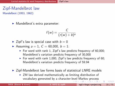
Zipf-Mandelbrot lawMandelbrot (1953, 1962)

I Mandelbrot’s extra parameter:

f (w) =C

(r(w) + b)a

I Zipf’s law is special case with b = 0I Assuming a = 1, C = 60,000, b = 1:

I For word with rank 1, Zipf’s law predicts frequency of 60,000;Mandelbrot’s variation predicts frequency of 30,000

I For word with rank 1,000, Zipf’s law predicts frequency of 60;Mandelbrot’s variation predicts frequency of 59.94

I Zipf-Mandelbrot law forms basis of statistical LNRE modelsI ZM law derived mathematically as limiting distribution of

vocabulary generated by a character-level Markov process



Zipf-Mandelbrot vs. Zipf’s lawNon-linear least-squares fit (Brown corpus)


Lexical statistics & word frequency distributions Some applications

Outline



zipfR



Applications of word frequency distributions

I Application 1: extrapolation of vocabulary size and frequencyspectrum to larger sample sizes

I morphological productivity (e.g. Lüdeling and Evert 2005)I lexical richness in stylometry (Efron and Thisted 1976),

language acquisition, clinical linguistics (Garrard et al. 2005)I language technology (estimate proportion of OOV words,

unseen grammar rules, typos, . . . )

+ need method for predicting vocab. growth on unseen data

I Application 2: Zipfian frequency distribution across typesI measures of lexical richness based on population (6= sample)I population model for Good-Turing smoothing (Good 1953;

Gale and Sampson 1995)I realistic prior for Bayesian language modelling

+ need model of type probability distribution in the population



Vocabulary growth: Pronouns vs. ri- in Italian

N V (pron.) V (ri-)5000 67 224

10000 69 27115000 69 28820000 70 30025000 70 32230000 71 34735000 71 36440000 71 37745000 71 38650000 71 400. . . . . . . . .



Vocabulary growth: Pronouns vs. ri- in ItalianVocabulary growth curves (V and V1)

0 2000 4000 6000 8000 10000

020

4060

80

N

V a

nd V

_1

0 200000 600000 10000000

200

400

600

800

1000

N

V a

nd V

_1


Statistical LNRE Models

LNRE models for word frequency distributions

I LNRE = large number of rare events (cf. Baayen 2001)I Statistics: corpus as random sample from population

I population characterised by vocabulary of types wk withoccurrence probabilities πk

I not interested in specific types Ü arrange by decreasingprobability: π1 ≥ π2 ≥ π3 ≥ · · ·

I NB: not necessarily identical to Zipf ranking in sample!

I LNRE model = population model for type probabilities, i.e. afunction k 7→ πk (with small number of parameters)

I type probabilities πk cannot be estimated reliably from acorpus, but parameters of LNRE model can

å Parametric statistical model



Examples of population models

●●●●

●

●

●

●

●

●

●

●

●

●

●

●

●

●

●●

●●

●●

●●●●●●●●●●●●●●●●●●

0 10 20 30 40 50

0.00

0.02

0.04

0.06

0.08

0.10

k

ππ k

●

●

●

●

●

●

●

●

●

●●

●●

●●

●●●●●●●●●●●●●●●●●●●●●●●●●●●●●●●●●●●

0 10 20 30 40 50

0.00

0.02

0.04

0.06

0.08

0.10

k

ππ k●

●

●

●

●

●

●●

●●

●●

●●

●●●●●●●●●●●●●●●●●●●●●●●●●●●●●●●●●●●●

0 10 20 30 40 50

0.00

0.02

0.04

0.06

0.08

0.10

k

ππ k

●

●

●

●

●

●

●

●

●

●

●

●●

●●

●●

●●

●●●●●●●●●●●●●●●●●●●●●●●●●●●●●●●

0 10 20 30 40 50

0.00

0.02

0.04

0.06

0.08

0.10

k

ππ k



The Zipf-Mandelbrot law as a population model

What is the right family of models for lexical frequencydistributions?

I We have already seen that the Zipf-Mandelbrot law capturesthe distribution of observed frequencies very well

I Re-phrase the law for type probabilities:

πk :=C

(k + b)a

I Two free parameters: a > 1 and b ≥ 0I C is not a parameter but a normalization constant,

needed to ensure that∑

k πk = 1I This is the Zipf-Mandelbrot population model


Statistical LNRE Models ZM & fZM

Outline



zipfR



The parameters of the Zipf-Mandelbrot model●

●

●

●

●

●

●●

●●

●●●●●●●●●●●●●●●●●●●●●●●●●●●●●●●●●●●●●●●●

0 10 20 30 40 50

0.00

0.02

0.04

0.06

0.08

0.10

k

ππ k

a == 1.2b == 1.5

●

●

●

●

●

●

●

●

●

●●

●●

●●

●●●●●●●●●●●●●●●●●●●●●●●●●●●●●●●●●●●

0 10 20 30 40 50

0.00

0.02

0.04

0.06

0.08

0.10

k

ππ k

a == 2b == 10

●

●

●

●

●

●

●●

●●

●●

●●

●●●●●●●●●●●●●●●●●●●●●●●●●●●●●●●●●●●●

0 10 20 30 40 50

0.00

0.02

0.04

0.06

0.08

0.10

k

ππ k

a == 2b == 15

●

●

●

●

●

●

●

●

●

●

●

●●

●●

●●

●●

●●●●●●●●●●●●●●●●●●●●●●●●●●●●●●●

0 10 20 30 40 50

0.00

0.02

0.04

0.06

0.08

0.10

k

ππ k

a == 5b == 40



The parameters of the Zipf-Mandelbrot model●

●

●

●

●●

●●

●●

●●●●●●●●●●●●●●●●●●●●●●●●●●●●●●●●●●●●●●●●●●●●●●●●●●●●●●●●●●●●●●●●●●●●●●●●●●●●●●●●●●●●●●●●●●●●●●●●●●●●●●●●●●●●●●●●●●●●●●●●●●●●●●●●●●●●●●●●●●●●●●●●●●●●●●●●●●●●●●●●●●●●●●●●●●●●●●●●●●●●●●●●●●●●●●●●●●●●●●●●●●●●●●●●●●●●●●●●●●●●●●●●●●●●●●●●●●●●●●●●●●●●●●●●●●●●●●●●●●●●●●●●●●●●●●●●●●●●●●●●●●●●●●●●●●●●●●●●●●●●●●●●●●●●●●●●●●●●●●●●●●●●●●●●●●●●●●●●●●●●●●●●●●●●●●●●●●●●●●●●●●●●●●●●●●●●●●●●●●●●●●●●●●●●●●●●●●●●●●●●●●●●●●●●●●●●●●●●●●●●●●●●●●●●●●●●●●●●●●●●●●●●●●●●●●●●●●●●●●●●●●●●●●●●●●●●●●●●●●●●●●●●●●●●●●

1 2 5 10 20 50 100

1e−

045e

−04

5e−

035e

−02

k

ππ k

a == 1.2b == 1.5

●●

●●

●●

●●

●●

●●●●●●●●●●●●●●●●●●●●●●●●●●●●●●●●●●●●●●●●●●●●●●●●●●●●●●●●●●●●●●●●●●●●●●●●●●●●●●●●●●●●●●●●●●●●●●●●●●●●●●●●●●●●●●●●●●●●●●●●●●●●●●●●●●●●●●●●●●●●●●●●●●●●●●●●●●●●●●●●●●●●●●●●●●●●●●●●●●●●●●●●●●●●●●●●●●●●●●●●●●●●●●●●●●●●●●●●●●●●●●●●●●●●●●●●●●●●●●●●●●●●●●●●●●●●●●●●●●●●●●●●●●●●●●●●●●●●●●●●●●●●●●●●●●●●●●●●●●●●●●●●●●●●●●●●●●●●●●●●●●●●●●●●●●●●●●●●●●●●●●●●●●●●●●●●●●●●●●●●●●●●●●●●●●●●●●●●●●●●●●●●●●●●●●●●●●●●●●●●●●●●●●●●●●●●●●●●●●●●●●●●●●●●●●●●●●●●●●●●●●●●●●●●●●●●●●●●●●●●●●●●●●●●●●●●●●●●●●●●●●●●●●●●●●

1 2 5 10 20 50 100

1e−

045e

−04

5e−

035e

−02

k

ππ k

a == 2b == 10

●●

●●

●●

●●

●●

●●●●●●●●●●●●●●●●●●●●●●●●●●●●●●●●●●●●●●●●●●●●●●●●●●●●●●●●●●●●●●●●●●●●●●●●●●●●●●●●●●●●●●●●●●●●●●●●●●●●●●●●●●●●●●●●●●●●●●●●●●●●●●●●●●●●●●●●●●●●●●●●●●●●●●●●●●●●●●●●●●●●●●●●●●●●●●●●●●●●●●●●●●●●●●●●●●●●●●●●●●●●●●●●●●●●●●●●●●●●●●●●●●●●●●●●●●●●●●●●●●●●●●●●●●●●●●●●●●●●●●●●●●●●●●●●●●●●●●●●●●●●●●●●●●●●●●●●●●●●●●●●●●●●●●●●●●●●●●●●●●●●●●●●●●●●●●●●●●●●●●●●●●●●●●●●●●●●●●●●●●●●●●●●●●●●●●●●●●●●●●●●●●●●●●●●●●●●●●●●●●●●●●●●●●●●●●●●●●●●●●●●●●●●●●●●●●●●●●●●●●●●●●●●●●●●●●●●●●●●●●●●●●●●●●●●●●●●●●●●●●●●●●●●●●1 2 5 10 20 50 100

1e−

045e

−04

5e−

035e

−02

k

ππ k

a == 2b == 15

●●

●●

●●

●●

●●

●●●●●●●●●●●●●●●●●●●●●●●●●●●●●●●●●●●●●●●●●●●●●●●●●●●●●●●●●●●●●●●●●●●●●●●●●●●●●●●●●●●●●●●●●●●●●●●●●●●●●●●●●●●●●●●●●●●●●●●●●●●●●●●●●●●●●●●●●●●●●●●●●●●●●●●●●●●●●●●●●●●●●●●●●●●●●●●●●●●●

1 2 5 10 20 50 100

1e−

045e

−04

5e−

035e

−02

k

ππ k

a == 5b == 40



The finite Zipf-Mandelbrot model

I Zipf-Mandelbrot population model characterizes an infinitetype population: there is no upper bound on k , and the typeprobabilities πk can become arbitrarily small

I π = 10−6 (once every million words), π = 10−9 (once everybillion words), π = 10−15 (once on the entire Internet),π = 10−100 (once in the universe?)

I Alternative: finite (but often very large) numberof types in the population

I We call this the population vocabulary size S(and write S =∞ for an infinite type population)



The finite Zipf-Mandelbrot modelEvert (2004)

I The finite Zipf-Mandelbrot model simply stops after the firstS types (w1, . . . ,wS)

I S becomes a new parameter of the model→ the finite Zipf-Mandelbrot model has 3 parameters

Abbreviations:I ZM for Zipf-Mandelbrot modelI fZM for finite Zipf-Mandelbrot model


Statistical LNRE Models Sampling from a LNRE model

Outline



zipfR



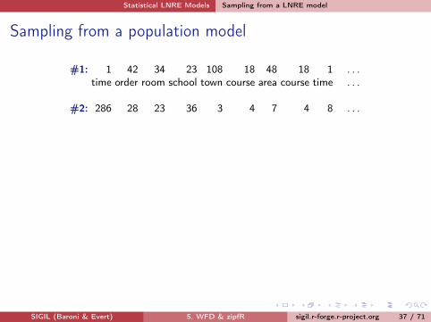
Sampling from a population model

Assume we believe that the population we are interested in can bedescribed by a Zipf-Mandelbrot model:

●

●

●

●

●

●

●●

●●

●●

●●

●●

●●

●●

●●●●●●●●●●●●●●●●●●●●●●●●●●●●●●

0 10 20 30 40 50

0.00

0.01

0.02

0.03

0.04

0.05

k

ππ k

a == 3b == 50

● ● ● ● ● ● ●●●●●●●●●●●●●●●●●●●●●●●●●●●●●●●●●●●●●●●●●●●●●●●●●●●●●●●●●●●●●●●●●●●●●●●●●●●●●●●●●●●●●●●●●●●●●●●●●●●●●●●●●●●●●●●●●●●●●●●●●●●●●●●●●●●●●●●●●●●●●●●●●●●●●●●●●●●●●●●●●●●●●●●●●●●●●●●●●●●●●●●●●●●●●●●●●●●●●●●●●●●●●●●●●●●●●●●●●●●●●●●●●●●●●●●●●●●●●●●●●●●●●●●●●●●●●●●●●●●●●●●●●●●●●●●●●●●●●●●●●●●●●●●●●●●●●●●●●●●●●●●●●●●●●●●●●●●●●●●●●●●●●●●●●●●●●●●●●●●●●●●●●●●●●●●●●●●●●●●●●●●●●●●●●●●●●●●●●●●●●●●●●●●●●●●●●●●●●●●●●●●●●●●●●●●●●●●●●●●●●●●●●●●●●●●●●●●●●●●●●●●●●●●●●●●●●●●●●●●●●●●●●●●●●●●●●●●●●●●●●●●●●●●●●●●●●●

1 2 5 10 20 50 100

1e−

045e

−04

5e−

035e

−02

k

ππ k

a == 3b == 50

Use computer simulation to sample from this model:I Draw N tokens from the population such that in

each step, type wk has probability πk to be pickedI This allows us to make predictions for samples (= corpora) of

arbitrary size N Ü extrapolationSIGIL (Baroni & Evert) 5. WFD & zipfR sigil.r-forge.r-project.org 36 / 71



#1: 1 42 34 23 108 18 48 18 1 . . .

time order room school town course area course time . . .

#2: 286 28 23 36 3 4 7 4 8 . . .

#3: 2 11 105 21 11 17 17 1 16 . . .

#4: 44 3 110 34 223 2 25 20 28 . . .

#5: 24 81 54 11 8 61 1 31 35 . . .

#6: 3 65 9 165 5 42 16 20 7 . . .

#7: 10 21 11 60 164 54 18 16 203 . . .

#8: 11 7 147 5 24 19 15 85 37 . . .

......

......

......

......

......




#1: 1 42 34 23 108 18 48 18 1 . . .time order room school town course area course time . . .

#2: 286 28 23 36 3 4 7 4 8 . . .

#3: 2 11 105 21 11 17 17 1 16 . . .

#4: 44 3 110 34 223 2 25 20 28 . . .

#5: 24 81 54 11 8 61 1 31 35 . . .

#6: 3 65 9 165 5 42 16 20 7 . . .

#7: 10 21 11 60 164 54 18 16 203 . . .

#8: 11 7 147 5 24 19 15 85 37 . . .

......

......

......

......

......



Samples: type frequency list & spectrum

rank r fr type k

1 37 62 36 13 33 34 31 75 31 106 30 57 28 128 27 29 24 410 24 1611 23 812 22 14...

......

m Vm

1 832 223 204 125 106 57 58 39 3

10 3...

...

sample #1



Samples: type frequency list & spectrum

rank r fr type k

1 39 22 34 33 30 54 29 105 28 86 26 17 25 138 24 79 23 610 23 1111 20 412 19 17...

......

m Vm

1 762 273 174 105 66 57 78 3

10 411 2...

...

sample #2



Random variation in type-frequency lists●

●

●

●●●

●●

●●●

●●

●●

●●●

●●

●●●●●●

●●●●

●●●●●●

●●●●●●●●●●

●●●●

0 10 20 30 40 50

010

2030

40

Sample #1

r

f r●

●

●●

●

●●

●●●

●●●

●●●●●●●

●●●●

●●

●●●●●

●●●●

●●●●●●●●●●

●●●●●

0 10 20 30 40 50

010

2030

40

Sample #2

r

f r

r ↔ fr

●

●

●

●

●

●

●

●

●

●

●

●

●

●●

●

●

●

●●

●

●

●●

●●

●

●●

●

●

●●

●

●

●

●

●

●

●

●●

●●

●

●●●

●●

0 10 20 30 40 50

010

2030

40

Sample #1

k

f k

●

●

●

●

●

●●

●

●

●

●

●

●

●●

●

●

●

●

●

●●

●

●

●●

●

●

●

●

●●●

●●

●

●

●

●

●

●

●

●●

●●

●

●

●

●

0 10 20 30 40 50

010

2030

40

Sample #2

k

f k

k ↔ fk



Random variation: frequency spectrum

Sample #1

m

Vm

020

4060

8010

0




Sample #2

m

Vm

020

4060

8010

0




Sample #3

m

Vm

020

4060

8010

0




Sample #4

m

Vm

020

4060

8010

0



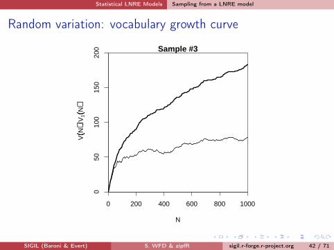
Random variation: vocabulary growth curve

0 200 400 600 800 1000

050

100

150

200 Sample #1

N

V((N

))V

1((N

))




0 200 400 600 800 1000

050

100

150

200 Sample #2

N

V((N

))V

1((N

))




0 200 400 600 800 1000

050

100

150

200 Sample #3

N

V((N

))V

1((N

))




0 200 400 600 800 1000

050

100

150

200 Sample #4

N

V((N

))V

1((N

))


Statistical LNRE Models Great expectations

Outline



zipfR



Expected values

I There is no reason why we should choose a particular sampleto make a prediction for the real data – each one is equallylikely or unlikely

I Take the average over a large number of samples, calledexpected value or expectation in statistics

I Notation: E[V (N)

]and E

[Vm(N)

]I indicates that we are referring to expected values for a sample

of size NI rather than to the specific values V and Vm

observed in a particular sample or a real-world data set

I Expected values can be calculated efficiently withoutgenerating thousands of random samples



The expected frequency spectrum

Vm

E[[Vm]]

Sample #1

m

Vm

E[[V

m]]

020

4060

8010

0




Vm

E[[Vm]]

Sample #2

m

Vm

E[[V

m]]

020

4060

8010

0




Vm

E[[Vm]]

Sample #3

m

Vm

E[[V

m]]

020

4060

8010

0




Vm

E[[Vm]]

Sample #4

m

Vm

E[[V

m]]

020

4060

8010

0



The expected vocabulary growth curve

0 200 400 600 800 1000

050

100

150

200 Sample #1

N

E[[V

((N))]]

V((N))E[[V((N))]]

0 200 400 600 800 1000

050

100

150

200 Sample #1

NE

[[V1((

N))]]

V1((N))E[[V1((N))]]



Prediction intervals for the expected VGC

0 200 400 600 800 1000

050

100

150

200 Sample #1

N

E[[V

((N))]]

V((N))E[[V((N))]]

0 200 400 600 800 1000

050

100

150

200 Sample #1

NE

[[V1((

N))]]

V1((N))E[[V1((N))]]

“Confidence intervals” that indicate predicted sampling distribution:+ for 95% of samples generated by the LNRE model, VGC will

fall within the range delimited by the thin red lines


Statistical LNRE Models Parameter estimation for LNRE models

Outline



zipfR



Parameter estimation by trial & error

observedZM model

a == 1.5,, b == 7.5

m

Vm

E[[V

m]]

050

0010

000

1500

020

000

2500

0

0e+00 2e+05 4e+05 6e+05 8e+05 1e+06

010

000

2000

030

000

4000

050

000 a == 1.5,, b == 7.5

N

V((N

))E

[[V((N

))]]

observedZM model




observedZM model

a == 1.3,, b == 7.5

m

Vm

E[[V

m]]

050

0010

000

1500

020

000

2500

0

0e+00 2e+05 4e+05 6e+05 8e+05 1e+06

010

000

2000

030

000

4000

050

000 a == 1.3,, b == 7.5

N

V((N

))E

[[V((N

))]]

observedZM model




observedZM model

a == 1.3,, b == 0.2

m

Vm

E[[V

m]]

050

0010

000

1500

020

000

2500

0

0e+00 2e+05 4e+05 6e+05 8e+05 1e+06

010

000

2000

030

000

4000

050

000 a == 1.3,, b == 0.2

N

V((N

))E

[[V((N

))]]

observedZM model




observedZM model

a == 1.5,, b == 7.5

m

Vm

E[[V

m]]

050

0010

000

1500

020

000

2500

0

0e+00 2e+05 4e+05 6e+05 8e+05 1e+06

010

000

2000

030

000

4000

050

000 a == 1.5,, b == 7.5

N

V((N

))E

[[V((N

))]]

observedZM model




observedZM model

a == 1.7,, b == 7.5

m

Vm

E[[V

m]]

050

0010

000

1500

020

000

2500

0

0e+00 2e+05 4e+05 6e+05 8e+05 1e+06

010

000

2000

030

000

4000

050

000 a == 1.7,, b == 7.5

N

V((N

))E

[[V((N

))]]

observedZM model




observedZM model

a == 1.7,, b == 80

m

Vm

E[[V

m]]

050

0010

000

1500

020

000

2500

0

0e+00 2e+05 4e+05 6e+05 8e+05 1e+06

010

000

2000

030

000

4000

050

000 a == 1.7,, b == 80

N

V((N

))E

[[V((N

))]]

observedZM model




observedZM model

a == 2,, b == 550

m

Vm

E[[V

m]]

050

0010

000

1500

020

000

2500

0

0e+00 2e+05 4e+05 6e+05 8e+05 1e+06

010

000

2000

030

000

4000

050

000 a == 2,, b == 550

N

V((N

))E

[[V((N

))]]

observedZM model



Automatic parameter estimation

observedexpected

a == 2.39,, b == 1968.49

m

Vm

E[[V

m]]

050

0010

000

1500

020

000

2500

0

0e+00 2e+05 4e+05 6e+05 8e+05 1e+06

010

000

2000

030

000

4000

050

000 a == 2.39,, b == 1968.49

N

V((N

))E

[[V((N

))]]

observedexpected

I By trial & error we found a = 2.0 and b = 550I Automatic estimation procedure: a = 2.39 and b = 1968


Statistical LNRE Models Reliability

Outline



zipfR



Goodness-of-fit

I Goodness-of-fit statistics measure how well the model hasbeen fitted to the observed training data

I Compare observed vs. expected frequency distributionI frequency spectrum (Ü easier)I vocabulary growth curve

I Similarity measuresI mean square error (Ü dominated by large V / Vm)I multivariate chi-squared statistic X 2 takes sampling variation

(and covariance of spectrum elements) into accountI Multivariate chi-squared test for goodness-of-fit

I H0 : observed data = sample from LNRE model(i.e. fitted LNRE model describes the true population)

I p-value derived from X 2 statistic (X 2 ∼ χdf under H0)I in previous example: p ≈ 0 :-(



Goodness-of-fit




(and covariance of spectrum elements) into account

I Multivariate chi-squared test for goodness-of-fitI H0 : observed data = sample from LNRE model

(i.e. fitted LNRE model describes the true population)I p-value derived from X 2 statistic (X 2 ∼ χdf under H0)I in previous example: p ≈ 0 :-(



Goodness-of-fit




(and covariance of spectrum elements) into accountI Multivariate chi-squared test for goodness-of-fit

I H0 : observed data = sample from LNRE model(i.e. fitted LNRE model describes the true population)

I p-value derived from X 2 statistic (X 2 ∼ χdf under H0)I in previous example: p ≈ 0 :-(



How reliable are the fitted models?

Three potential issues:

1. Model assumptions 6= population(e.g. distribution does not follow a Zipf-Mandelbrot law)

+ model cannot be adequate, regardless of parameter settings

2. Parameter estimation unsuccessful(i.e. suboptimal goodness-of-fit to training data)

+ optimization algorithm trapped in local minimum+ can result in highly inaccurate model

3. Uncertainty due to sampling variation(i.e. observed training data differ from population distribution)

+ model fitted to training data, may not reflect true population+ another training sample would have led to different parameters



How reliable are the fitted models?

Three potential issues:1. Model assumptions 6= population

(e.g. distribution does not follow a Zipf-Mandelbrot law)+ model cannot be adequate, regardless of parameter settings

2. Parameter estimation unsuccessful(i.e. suboptimal goodness-of-fit to training data)

+ optimization algorithm trapped in local minimum+ can result in highly inaccurate model

3. Uncertainty due to sampling variation(i.e. observed training data differ from population distribution)

+ model fitted to training data, may not reflect true population+ another training sample would have led to different parameters



Bootstrapping

I An empirical approach to sampling variation:I take many random samples from the same populationI estimate LNRE model from each sampleI analyse distribution of model parameters, goodness-of-fit, etc.

(mean, median, s.d., boxplot, histogram, . . . )I problem: how to obtain the additional samples?

I Bootstrapping (Efron 1979)I resample from observed data with replacementI this approach is not suitable for type-token distributions

(resamples underestimate vocabulary size V !)I Parametric bootstrapping

I use fitted model to generate samples, i.e. sample from thepopulation described by the model

I advantage: “correct” parameter values are known



Bootstrapping




(resamples underestimate vocabulary size V !)

I Parametric bootstrappingI use fitted model to generate samples, i.e. sample from the

population described by the modelI advantage: “correct” parameter values are known



Bootstrapping




(resamples underestimate vocabulary size V !)I Parametric bootstrapping

I use fitted model to generate samples, i.e. sample from thepopulation described by the model

I advantage: “correct” parameter values are known



Bootstrappingparametric bootstrapping with 100 replicates

Zipfian slope a = 1/α

0.0 0.2 0.4 0.6 0.8 1.0

02

46

810

12

α

Den

sity




Offset b = (1− α)/(B · α)

0.0 0.2 0.4 0.6 0.8 1.0

05

1015

B

Den

sity




fZM probability cutoff A = πS

0.0e+00 5.0e−06 1.0e−05 1.5e−05 2.0e−05

050

000

1500

00

A

Den

sity




Goodness-of-fit statistic X 2 (model not plausible for X 2 > 11)

0 5 10 15 20 25 30

0.00

0.02

0.04

0.06

0.08

X2

Den

sity

p<

0.05




Population vocabulary size S

0e+00 2e+21 4e+21 6e+21

0e+

002e

−05

4e−

056e

−05

S

Den

sity




Population vocabulary size S

0e+00 2e+04 4e+04 6e+04 8e+04 1e+05

0e+

002e

−05

4e−

05

S

Den

sity



Summary

LNRE modelling in a nutshell:

1. Compile observed frequency spectrum (and vocabularygrowth curves) for a given corpus or data set

2. Estimate parameters of LNRE model by matching observedand expected frequency spectrum

3. Evaluate goodness-of-fit on spectrum (Baayen 2001) or bytesting extrapolation accuracy (Baroni and Evert 2007)

I in principle, you should only go on if model gives a plausibleexplanation of the observed data!

4. Use LNRE model to compute expected frequency spectrumfor arbitrary sample sizesÜ extrapolation of vocabulary growth curve

I or use population model directly as Bayesian prior etc.



Summary

LNRE modelling in a nutshell:1. Compile observed frequency spectrum (and vocabulary

growth curves) for a given corpus or data set

2. Estimate parameters of LNRE model by matching observedand expected frequency spectrum







Summary


growth curves) for a given corpus or data set2. Estimate parameters of LNRE model by matching observed

and expected frequency spectrum







Summary


growth curves) for a given corpus or data set2. Estimate parameters of LNRE model by matching observed

and expected frequency spectrum3. Evaluate goodness-of-fit on spectrum (Baayen 2001) or by

testing extrapolation accuracy (Baroni and Evert 2007)I in principle, you should only go on if model gives a plausible

explanation of the observed data!




zipfR

zipfREvert and Baroni (2007)

I http://zipfR.R-Forge.R-Project.org/I Conveniently available from CRAN repository

I see Unit 1 for general package installation guides


http://zipfR.R-Forge.R-Project.org/

zipfR

Loading

> library(zipfR)

> ?zipfR

> data(package="zipfR")

# package overview in HTML help leads to zipfR tutorial> help.start()


zipfR

Importing data

> data(ItaRi.spc) # not necessary in recent package versions> data(ItaRi.emp.vgc)

# load your own data sets (see ?read.spc etc. for file format)> my.spc <- read.spc("my.spc.txt")> my.vgc <- read.vgc("my.vgc.txt")

> my.tfl <- read.tfl("my.tfl.txt")> my.spc <- tfl2spc(my.tfl) # compute spectrum from frequency list


zipfR

Looking at spectra

> summary(ItaRi.spc)> ItaRi.spc

> N(ItaRi.spc)> V(ItaRi.spc)> Vm(ItaRi.spc, 1)> Vm(ItaRi.spc, 1:5)

# Baayen’s P = estimate for slope of VGC> Vm(ItaRi.spc, 1) / N(ItaRi.spc)

> plot(ItaRi.spc)> plot(ItaRi.spc, log="x")


zipfR

Looking at VGCs

> summary(ItaRi.emp.vgc)> ItaRi.emp.vgc

> N(ItaRi.emp.vgc)

> plot(ItaRi.emp.vgc, add.m=1)


zipfR

Smoothing VGCs with binomial interpolation(for details, see Baayen 2001, Sec. 2.6.1)

# interpolated VGC> ItaRi.bin.vgc <-

vgc.interp(ItaRi.spc, N(ItaRi.emp.vgc), m.max=1)

> summary(ItaRi.bin.vgc)

# comparison> plot(ItaRi.emp.vgc, ItaRi.bin.vgc,

legend=c("observed", "interpolated"))


zipfR

ultra-

I Load the spectrum and empirical VGC of the less commonprefix ultra-

I Compute binomially interpolated VGC for ultra-I Plot the binomially interpolated ri- and ultra- VGCs together


zipfR

Estimating LNRE models

# fit a fZM model# (you can also try ZM and GIGP, and compare them with fZM)

> ItaUltra.fzm <- lnre("fzm", ItaUltra.spc)

> summary(ItaUltra.fzm)


zipfR

Observed/expected spectra at estimation size

# expected spectrum> ItaUltra.fzm.spc <-

lnre.spc(ItaUltra.fzm, N(ItaUltra.fzm))

# compare> plot(ItaUltra.spc, ItaUltra.fzm.spc,

legend=c("observed", "fzm"))

# plot first 10 elements only> plot(ItaUltra.spc, ItaUltra.fzm.spc,

legend=c("observed", "fzm"), m.max=10)


zipfR

Compare growth of two categories

# extrapolation of ultra- VGC to sample size of ri- data> ItaUltra.ext.vgc <-

lnre.vgc(ItaUltra.fzm, N(ItaRi.emp.vgc))

# compare> plot(ItaUltra.ext.vgc, ItaRi.bin.vgc,

N0=N(ItaUltra.fzm), legend=c("ultra-", "ri-"))

# zooming in> plot(ItaUltra.ext.vgc, ItaRi.bin.vgc,

N0=N(ItaUltra.fzm), legend=c("ultra-", "ri-"),xlim=c(0, 100e3))


zipfR

Model validation by parametric bootstrapping

# define function to extract relevant information from fitted model> extract.stats <- function (m)

data.frame(alpha=m$param$alpha, A=m$param$A,B=m$param$B, S=m$S, X2=m$gof$X2)

# run bootstrapping procedure (default = 100 replicates)> runs <- lnre.bootstrap(ItaUltra.fzm, N(ItaUltra.fzm),

lnre, extract.stats, type="fzm")

> head(runs)

# NB: don’t try this with large samples (N > 1M tokens)


zipfR

Model validation by parametric bootstrapping

# distribution of estimated model parameters> hist(runs$alpha, freq=FALSE, xlim=c(0, 1))> lines(density(runs$alpha), lwd=2, col="red")> abline(v=ItaUltra.fzm$param$alpha, lwd=2, col="blue")

# try the other parameters for yourself!

# distribution of goodness-of-fit values> hist(runs$X2, freq=FALSE)> lines(density(runs$X2), lwd=2, col="red")

# estimated population vocabulary size> hist(runs$S) # what is wrong here?


zipfR

References I

Baayen, R. Harald (2001). Word Frequency Distributions. Kluwer AcademicPublishers, Dordrecht.

Baroni, Marco (2008). Distributions in text. In A. Lüdeling and M. Kytö (eds.), CorpusLinguistics. An International Handbook, chapter 39. Mouton de Gruyter, Berlin.

Baroni, Marco and Evert, Stefan (2007). Words and echoes: Assessing and mitigatingthe non-randomness problem in word frequency distribution modeling. InProceedings of the 45th Annual Meeting of the Association for ComputationalLinguistics, pages 904–911, Prague, Czech Republic.

Efron, Bradley (1979). Bootstrap methods: Another look at the jackknife. The Annalsof Statistics, 7(1), 1–26.

Efron, Bradley and Thisted, Ronald (1976). Estimating the number of unseen species:How many words did Shakespeare know? Biometrika, 63(3), 435–447.

Evert, Stefan (2004). A simple LNRE model for random character sequences. InProceedings of the 7èmes Journées Internationales d’Analyse Statistique desDonnées Textuelles (JADT 2004), pages 411–422, Louvain-la-Neuve, Belgium.

Evert, Stefan and Baroni, Marco (2007). zipfR: Word frequency distributions in R. InProceedings of the 45th Annual Meeting of the Association for ComputationalLinguistics, Posters and Demonstrations Sessions, pages 29–32, Prague, CzechRepublic.


zipfR

References II

Gale, William A. and Sampson, Geoffrey (1995). Good-Turing frequency estimationwithout tears. Journal of Quantitative Linguistics, 2(3), 217–237.

Garrard, Peter; Maloney, Lisa M.; Hodges, John R.; Patterson, Karalyn (2005). Theeffects of very early alzheimer’s disease on the characteristics of writing by arenowned author. Brain, 128(2), 250–260.

Good, I. J. (1953). The population frequencies of species and the estimation ofpopulation parameters. Biometrika, 40(3/4), 237–264.

Lüdeling, Anke and Evert, Stefan (2005). The emergence of productive non-medical-itis. corpus evidence and qualitative analysis. In S. Kepser and M. Reis (eds.),Linguistic Evidence. Empirical, Theoretical, and Computational Perspectives, pages351–370. Mouton de Gruyter, Berlin.

Mandelbrot, Benoit (1953). An informational theory of the statistical structure oflanguages. In W. Jackson (ed.), Communication Theory, pages 486–502.Butterworth, London.

Mandelbrot, Benoit (1962). On the theory of word frequencies and on relatedMarkovian models of discourse. In R. Jakobson (ed.), Structure of Language andits Mathematical Aspects, pages 190–219. American Mathematical Society,Providence, RI.


zipfR

References III

Zipf, George Kingsley (1949). Human Behavior and the Principle of Least Effort.Addison-Wesley, Cambridge, MA.

Zipf, George Kingsley (1965). The Psycho-biology of Language. MIT Press,Cambridge, MA.


Word Frequency Distributions with the zipfR package - Stefan Evert

Documents

Transcript of Word Frequency Distributions with the zipfR package - Stefan Evert