Wireless Transmission Fundamentals (Physical Layer) Professor Honggang Wang Email:...
32
Wireless Transmission Fundamentals (Physical Layer) Professor Honggang Wang Email: [email protected]
-
Upload
yosef-troughton -
Category
Documents
-
view
222 -
download
0
Transcript of Wireless Transmission Fundamentals (Physical Layer) Professor Honggang Wang Email:...
Wireless Transmission Fundamentals (Physical Layer)
Professor Honggang Wang
Email: [email protected]
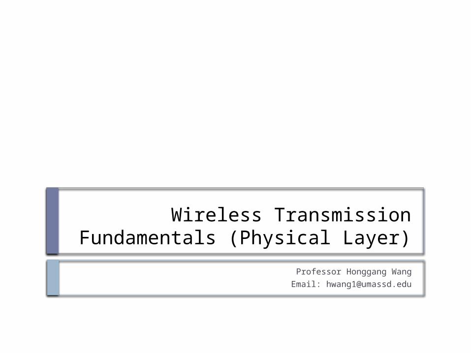
Electromagnetic Spectrum Wireless communication uses 100 kHz to 60
GHz
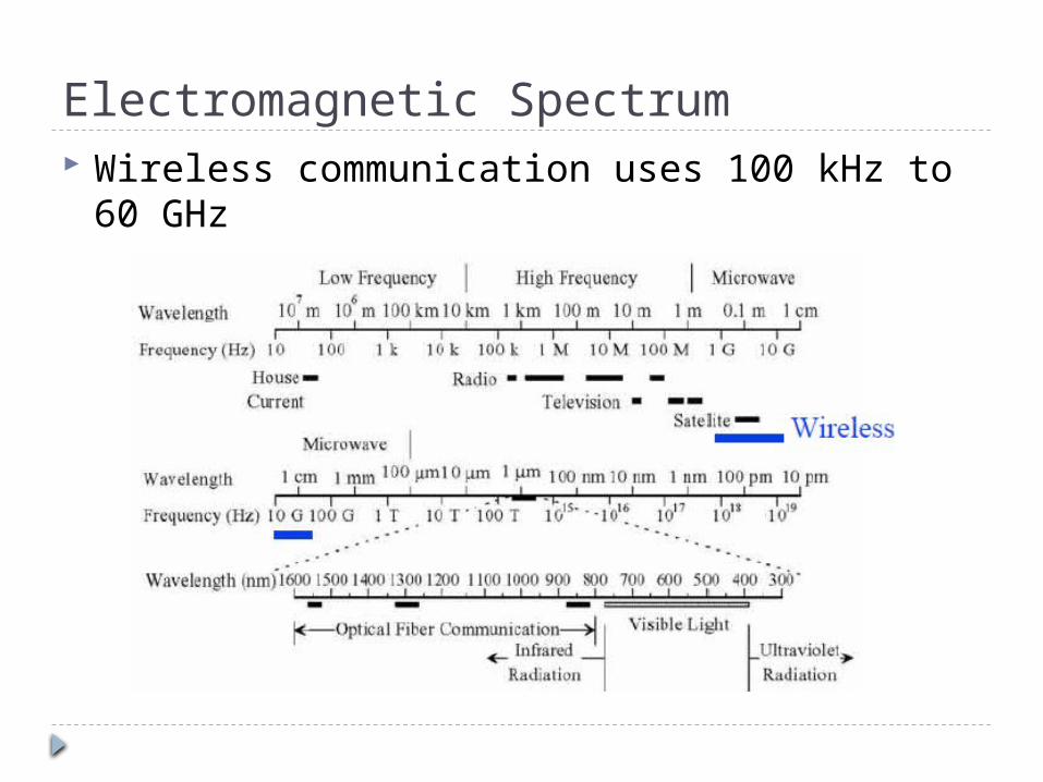
The Layered Reference Model
3
Application
Transport
Network
Data Link
Physical
Medium
Data Link
Physical
Application
Transport
Network
Data Link
Physical
Data Link
Physical
Network Network
Radio
Often we need to implement a function across multiple layers.

Outline RF introduction
Antennas and signal propagation How do antennas work Propagation properties of RF signals
Modulation and channel capacity
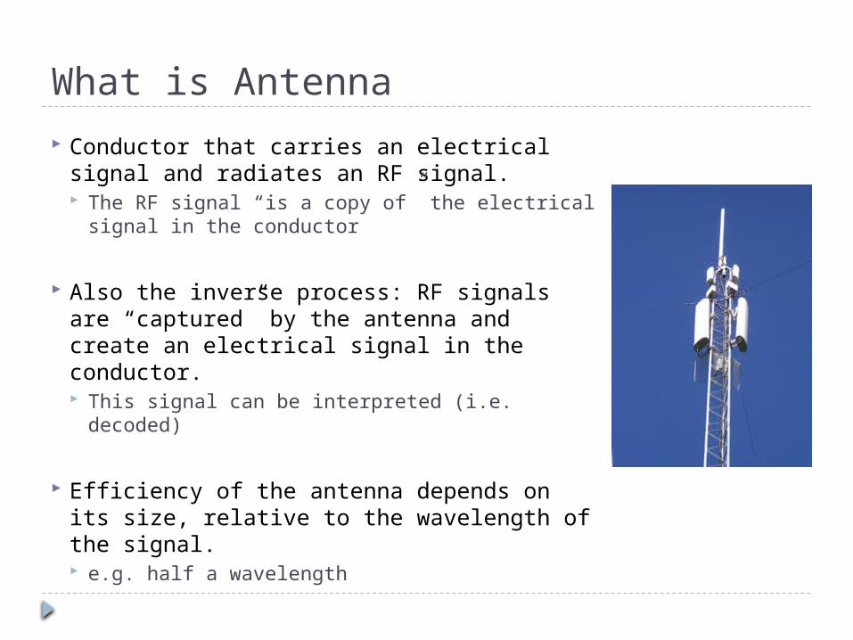
What is Antenna
Conductor that carries an electrical signal and radiates an RF signal. The RF signal “is a copy of” the electrical
signal in the conductor
Also the inverse process: RF signals are “captured” by the antenna and create an electrical signal in the conductor. This signal can be interpreted (i.e. decoded)
Efficiency of the antenna depends on its size, relative to the wavelength of the signal. e.g. half a wavelength

Types of Antennas Antenna is a point source that
radiates with the same power level in all directions – omni-directional or isotropic An antenna that transmits equally in all
directions (isotropic) Shape of the conductor tends to create
a specific radiation pattern Common shape is a straight
conductor Shaper antennas can be used to
direct the energy in a certain direction Well-know case: a parabolic antenna
A parabolic antenna
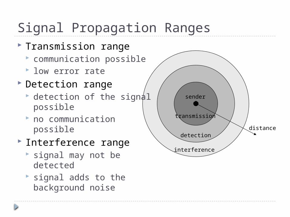
Signal Propagation Ranges Transmission range
communication possible low error rate
Detection range detection of the signal
possible no communication
possible Interference range
signal may not be detected
signal adds to the background noise
distance
sender
transmission
detection
interference

Signal propagation
Propagation in free space always like light (straight line) Receiving power proportional to 1/d² in vacuum – much more in real
environments(d = distance between sender and receiver)
Receiving power additionally influenced by fading (frequency dependent) Shadowing Reflection at large obstacles Refraction depending on the density of a medium Scattering at small obstacles Diffraction at edges
reflection scattering diffractionshadowing refraction

Propagation Degrades RF Signal
Attenuation in free space Signal gets weaker as it travels over
longer distance Free space loss- Signal spreads out Refraction and absorption in the
atmosphere Obstacle can weaken signal
through absorption or reflection. Part of the signal is re-directed.
Multiple path effects Multiple copies of the signal interfere
with each other Mobility
Moving receiver causes another form of self interference
Node moves ½ wavelength cause big change in signal strength
path loss
log (distance)
Received Signal
Power
(dB)
location

Decibels Attenuation = 10 Log10 (Pin/Pout) decibel Attenuation = 20 Log10 (Vin/Vout) decibel
Example 1: Pin = 10 mW, Pout=5 mW Attenuation = 10 log 10 (10/5) = 10 log 10 2 = 3
dB
Example 2: Pin = 100mW, Pout=1 mW Attenuation = 10 log 10 (100/1) = 10 log 10 100 =
20 dB
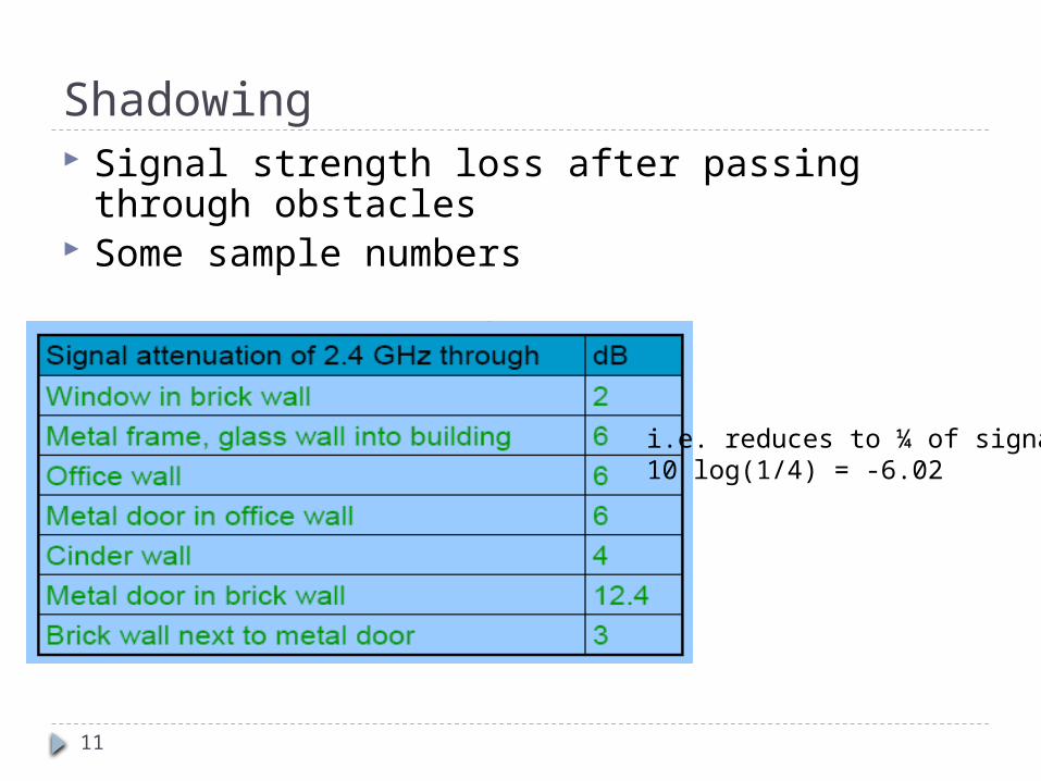
Shadowing
11
Signal strength loss after passing through obstacles
Some sample numbers
i.e. reduces to ¼ of signal10 log(1/4) = -6.02
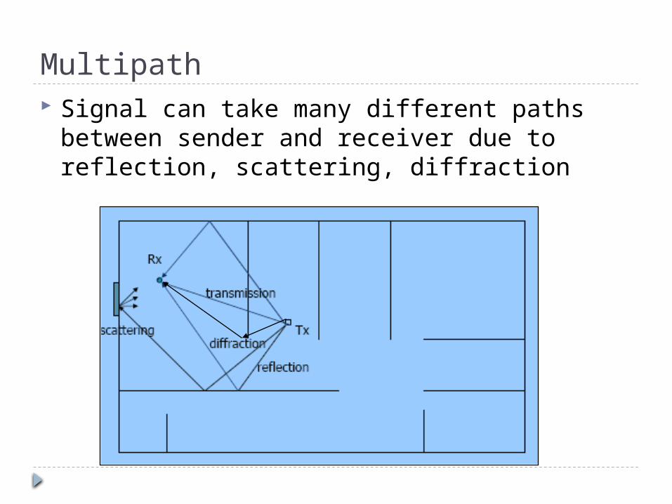
Multipath Signal can take many different paths between
sender and receiver due to reflection, scattering, diffraction

Multipath propagation Signal can take many different paths between sender
and receiver due to reflection, scattering, diffraction
Time dispersion: signal is dispersed over time interference with “neighbor” symbols, Inter Symbol
Interference (ISI) The signal reaches a receiver directly and phase shifted
distorted signal depending on the phases of the different parts
signal at sendersignal at receiver
LOS pulsesmultipathpulses
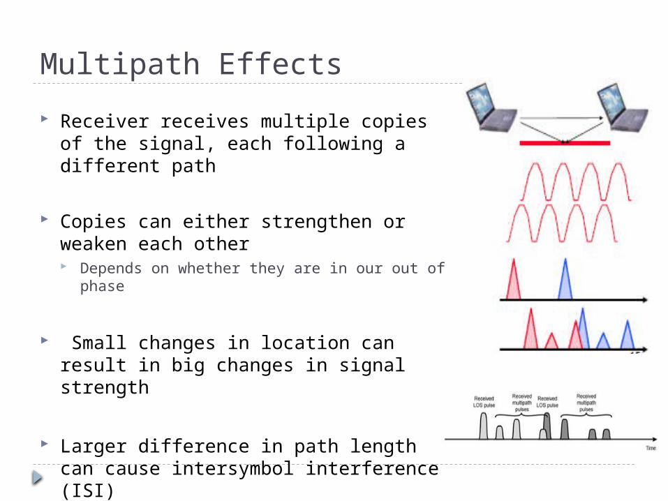
Multipath Effects
Receiver receives multiple copies of the signal, each following a different path
Copies can either strengthen or weaken each other Depends on whether they are in our out of phase
Small changes in location can result in big changes in signal strength
Larger difference in path length can cause intersymbol interference (ISI) More significant for higher bit rates (shorter bit
times)
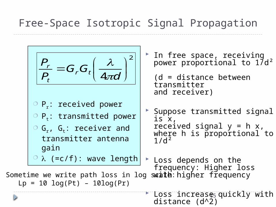
Free-Space Isotropic Signal Propagation
15
In free space, receiving power proportional to 1/d² (d = distance between transmitter and receiver)
Suppose transmitted signal is x,received signal y = h x, where h is proportional to 1/d²
Loss depends on the frequency: Higher loss with higher frequency
Loss increase quickly with distance (d^2)
2
4
dGG
P
Ptr
t
r
Pr: received power Pt: transmitted power Gr, Gt: receiver and
transmitter antenna gain (=c/f): wave length
Sometime we write path loss in log scale: Lp = 10 log(Pt) – 10log(Pr)

Outline RF introduction
Antennas and signal propagation How do antennas work Propagation properties of RF signals
Modulation and channel capacity

Signals Physical representation of data
Function of time and location
Signal parameters: parameters representing the value of data classification continuous time/discrete time continuous values/discrete values analog signal = continuous time and continuous values digital signal = discrete time and discrete values
Signal parameters of periodic signals: period T, frequency f=1/T, amplitude A, phase shift sine wave as special periodic signal for a carrier:
s(t) = At sin(2 ft t + t)
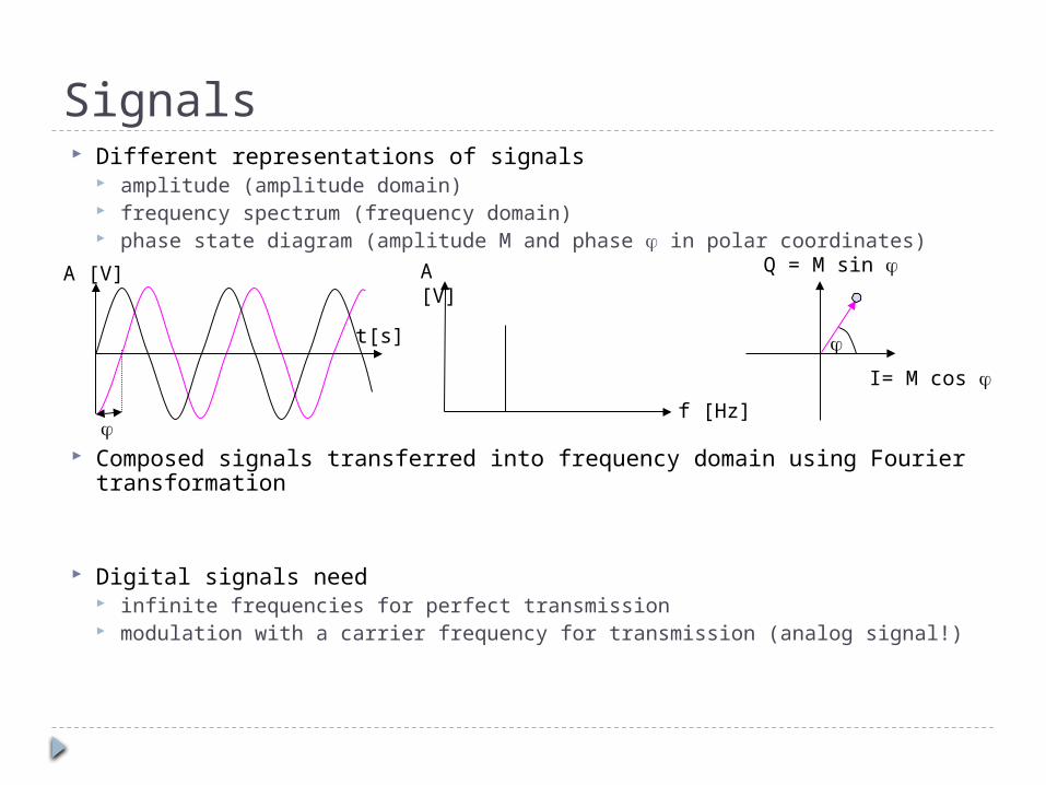
Signals Different representations of signals
amplitude (amplitude domain) frequency spectrum (frequency domain) phase state diagram (amplitude M and phase in polar coordinates)
Composed signals transferred into frequency domain using Fourier transformation
Digital signals need infinite frequencies for perfect transmission modulation with a carrier frequency for transmission (analog signal!)
f [Hz]
A [V]
I= M cos
Q = M sin
A [V]
t[s]

Multiplexing Multiplexing in 4 dimensions
space (si) time (t) frequency (f) code (c)
Goal: multiple use of a shared medium
Important: guard spaces needed!
s2
s3
s1f
t
ck2 k3 k4 k5 k6k1
f
t
c
f
t
c
channels ki
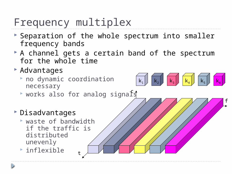
Frequency multiplex Separation of the whole spectrum into smaller
frequency bands A channel gets a certain band of the spectrum for
the whole time Advantages
no dynamic coordination necessary
works also for analog signals
Disadvantages waste of bandwidth
if the traffic is distributed unevenly
inflexible
k2 k3 k4 k5 k6k1
f
t
c
f
t
c
k2 k3 k4 k5 k6k1
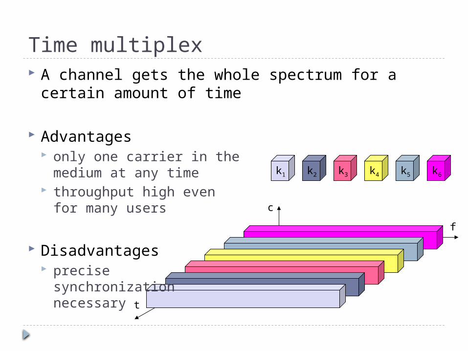
Time multiplex A channel gets the whole spectrum for a certain
amount of time
Advantages only one carrier in the
medium at any time throughput high even
for many users
Disadvantages precise
synchronization necessary
f
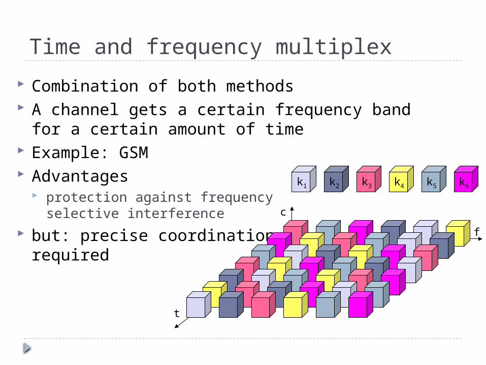
Time and frequency multiplex
Combination of both methods A channel gets a certain frequency band for a
certain amount of time Example: GSM Advantages
protection against frequency selective interference
but: precise coordinationrequired
t
c
k2 k3 k4 k5 k6k1
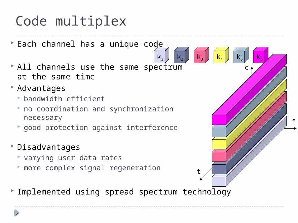
Code multiplex
Each channel has a unique code
All channels use the same spectrum at the same time
Advantages bandwidth efficient no coordination and synchronization
necessary good protection against interference
Disadvantages varying user data rates more complex signal regeneration
Implemented using spread spectrum technology
k2 k3 k4 k5 k6k1
f
t
c

Modulation Digital modulation
digital data is translated into an analog signal (baseband) ASK, FSK, PSK differences in spectral efficiency, power efficiency, robustness
Analog modulation shifts center frequency of baseband signal up to the radio carrier
Basic schemes Amplitude Modulation (AM) Frequency Modulation (FM) Phase Modulation (PM)

Modulation and Demodulation
synchronizationdecision
digitaldataanalog
demodulation
radiocarrier
analogbasebandsignal
101101001 radio receiver
digitalmodulation
digitaldata analog
modulation
radiocarrier
analogbasebandsignal
101101001 radio transmitter

Digital modulation
Modulation of digital signals known as Shift Keying
Amplitude Shift Keying (ASK): very simple low bandwidth requirements very susceptible to interference
Frequency Shift Keying (FSK): needs larger bandwidth
Phase Shift Keying (PSK): more complex robust against interference
1 0 1
t
1 0 1
t
1 0 1
t
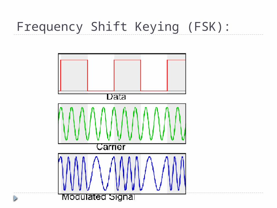
Frequency Shift Keying (FSK):
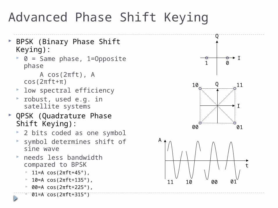
Advanced Phase Shift Keying
BPSK (Binary Phase Shift Keying): 0 = Same phase, 1=Opposite
phase A cos(2πft), A cos(2πft+π) low spectral efficiency robust, used e.g. in satellite
systems QPSK (Quadrature Phase Shift
Keying): 2 bits coded as one symbol symbol determines shift of
sine wave needs less bandwidth
compared to BPSK 11=A cos(2πft+45°), 10=A cos(2πft+135°), 00=A cos(2πft+225°), 01=A cos(2πft+315°)
11 10 00 01
Q
I01
Q
I
11
01
10
00
A
t

Quadrature Amplitude Modulation Quadrature Amplitude Modulation (QAM)
combines amplitude and phase modulation it is possible to code n bits using one symbol 2n discrete levels, n=2 identical to QPSK
Bit error rate increases with n, but less errors compared to comparable PSK schemes Example: 16-QAM (4 bits = 1 symbol) Symbols 0011 and 0001 have
the same phase φ, but differentamplitude
0000 and 1000 havedifferent phase, but same amplitude.
0000
0001
0011
1000
Q
I
0010
φ
a
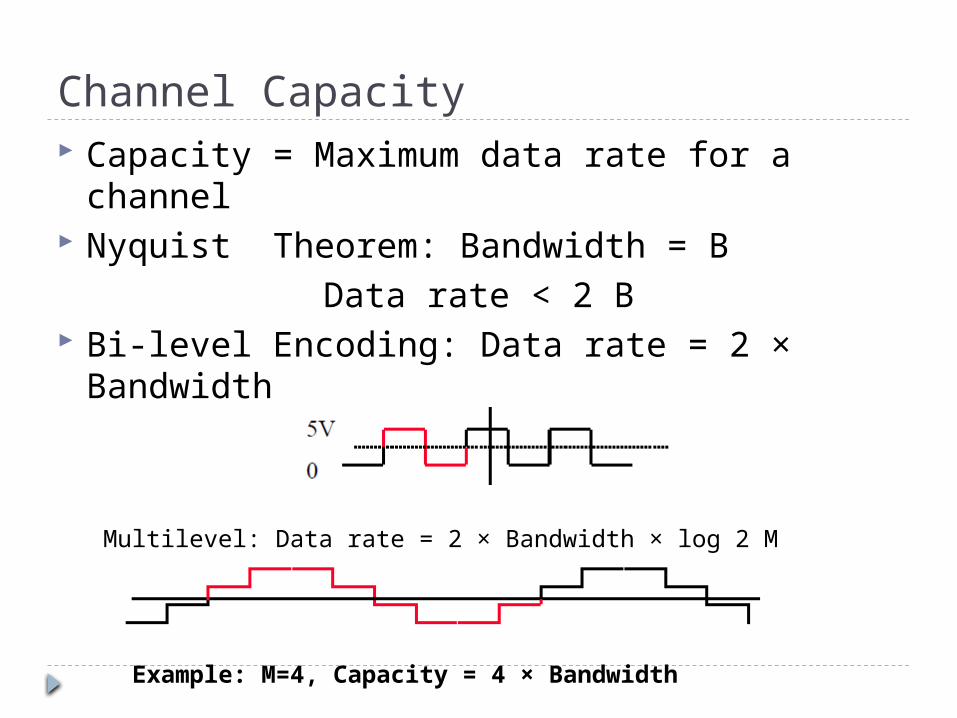
Channel Capacity Capacity = Maximum data rate for a channel Nyquist Theorem: Bandwidth = B
Data rate < 2 B Bi-level Encoding: Data rate = 2 × Bandwidth
Multilevel: Data rate = 2 × Bandwidth × log 2 M
Example: M=4, Capacity = 4 × Bandwidth
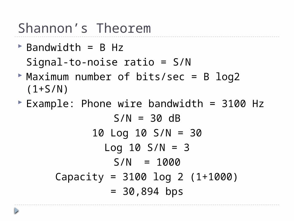
Shannon’s Theorem Bandwidth = B Hz Signal-to-noise ratio = S/N Maximum number of bits/sec = B log2 (1+S/N) Example: Phone wire bandwidth = 3100 Hz
S/N = 30 dB10 Log 10 S/N = 30
Log 10 S/N = 3S/N = 1000
Capacity = 3100 log 2 (1+1000)= 30,894 bps

Q/A
???