Wireless Propagation Effects in Highly Resonant

Environments

M. Panitz, P. Sewell, C. ChristopoulosGeorge Green Institute for Electromagnetics Research

The University of NottinghamAcknowledgement: MP is supported by an EPSRC/BAES Studentship

Introduction

• Why we want to minimise wires!

• Advantages of wireless systems-potential problems.

• Issues in wireless propagation.

• Channel models and BER-preliminary results.

• Reverberation chamber modelling-results.

• Vibration modeling

• Conclusions

Why are wires a problem?

• Current aircraft are controlled mainly by wires and some fibre-optic systems.

• Wire routing and fixing are not fully explored during the design process; wires become:

- Messy- Inaccessible- Inefficiently placed

• New technologies are being developed requiring large arrays of sensors and actuators so a reduction in wire usage is desired

• Copper wiring adds a significant amount of weight to an aircraft increasing fuel consumption and reducing flight range.

- JSF has over 28km wires and 20,000 connectors.

Concord wiring

JSF wiring

Advantages of wireless

• Improve safety - The large number of wires can degrade over time becoming a significant hazard due to the fatigue induced by vibrations bending, flexing, broken connections, battle damage etc. BUT, must be very reliable

• Allow a much larger number of sensors and actuators with minimalincrease in weight

• Provide more distributed aircraft system – Easier deployment of systems and much greater protection is guaranteed against single node failure

• Increased protection from lightning strike as there is no physical node to node connection

• Significantly reduce cost and weight due to wires- 747 has over 220km of wires weighing >1600kg

Resonance

• Transmitted power varies rapidly with frequency and a cut-off frequency is present

• A narrowband signal could fall into a transmission trough

0 0.5 1 1.5 2 2.5 3 3.5 4 4.5 5

x 109

-110

-100

-90

-80

-70

-60

-50

-40

-30

-20

-10

0

Frequency (Hz)

|S21

| (dB

)

Cylinder with Antenna 2mm mes h, Gaus s ian Input

dh

l1 l2 l3

z x

Simulated response of 45mm radius cylinder using TLM

S21 magnitude varies between -15 and -70dB across simulated frequency range

Multipath

• Multipath propagation causes delayed versions of a signal to be received with varying amplitudes

• The effect is common in communication channels e.g. mobile phones

• The effect in an enclosed metallic enclosure leads to resonances

0

0

( ) ( )

( ) ( )

N

n x nn

Nj

n xn

r t t t

R j T j e τω

α τ

ω α ω

=

=

= −

=

∑

∑Scattering

Tx Rx

ReflectionsReceived power from multipath

propagation in a metal box

0 0.2 0.4 0.6 0.8 1 1.2

x 10-6

-0.015

-0.01

-0.005

0

0.005

0.01

0.015

Time (s )

Amplitude

Q factor

• The Q factor tells us about the energy storage capability in an enclosure• A higher Q factor means more energy is stored per period• The response of same chamber with a different Q factor is shown• Q factor is frequency dependent and can be estimated from the energy

decay:

Or, in terms of the decay:

0

2

exp( )

avWQ f

E E t

fQ

πη

α

πα

=

= −

=

Delay Spread

• Delay spread used to quantify multipath interference

Meandelay

RMSdelay

• If the mean delay spread is of the order 1/10 the minimum data period then errors become significant

0.5 1 1.5 2 2.5

x 10-8

0

0.2

0.4

0.6

0.8

1

1.2

x 10-4

Time (s )

Magnitude

Time

Ampl

itude

0

0

( )

( )

gr

g

d

d

τφ τ τμ

φ τ τ

∞

∞= ∫∫

2

0

0

( ) ( )

( )

r gr

g

d

d

τ μ φ τ τσ

φ τ τ

∞

∞

−= ∫

∫

Modulation

Binary Phase Shift Keying

Quadrature Phase Shift Keying

Offset-quadrature Phase Shift Keying

Minimum Shift Keying

Spread spectrum

• It was shown that a conducting enclosure has a peaked response and signal transmission could coincide with a trough

• Intentionally and controllably spreading the signal out over a wider bandwidth could combat this problem

• There are two main techniques: DSSS and FHSS

t

t

t

Data:Period Td

Chip:Period Tc

Expansion factor = Tc / Td Frequency

DSSS FHSSCarrier frequency is varied randomly between a set number of discrete frequencies

( )( ) sin ( ) ( )S t A t t tω θ= +

Inputsignal

Spectrum ofinput signal

Spreadsignal

Spectrum ofspread signal

DSSS

• Initial investigations have been performed using the DSSS scheme, the effect of spreading can be seen here

• This scheme can be tested in the full-field TLM model, but this is slow. A more efficient model has been developed

Channel Modelling

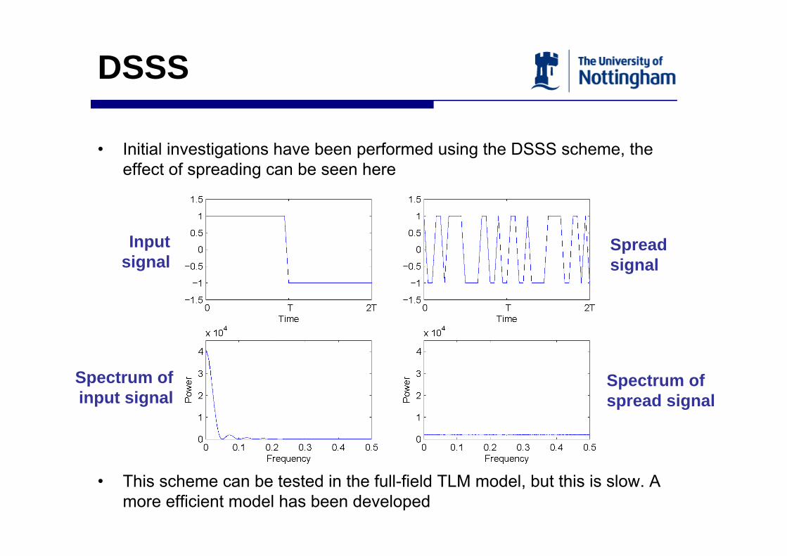
ωω0

Δω

A

A model is proposed to test the modulation and coding techniques in a channel with similar properties to those of the cavity structure.

Desired Properties:• Multiple peaks with direct control of frequency

and Q-factor.• An additional flat response for line of sight.• Fast, large sequences can be sent.

RDC

QNQ1

RN

CN

LN

R1

I

C1

V L1

Suggested Model:• Series RLC circuits in parallel to give

peaked response.• Single Resistor branch to give flat

response.• Use model to create a time-domain digital

filter for density of modes testing.

Resonant RLC response

Multi-resonance circuit model

Modelling (cont.)

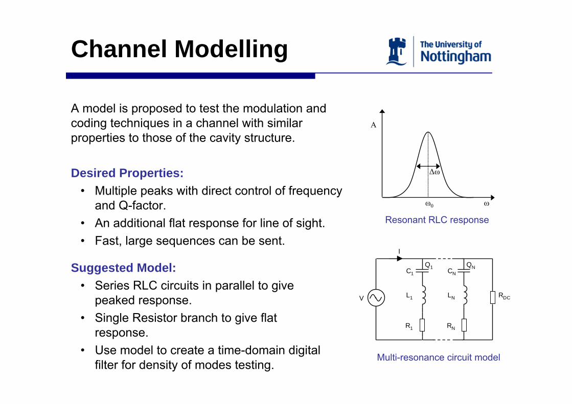
• Multipath delay and resonance are closely linked so should be included in the model

• The Q factor is determined by energy storage (or loss) of a chamber• The density of modes at a particular frequency is governed by the volume

and can be approximated by

• A good test is to calculate the Bit-Error-Ratio advantage offered with varied mode densities by using DSSS

• This can be performed at a number of Q factors and related to a real system where mode density and Q are known

2

3

8( ) Vfg fcπ

=

DSSS testing

The DSSS technique is tested in the channel by calculating a BER for an unspread and a spread signal passed though the channel.Signal Parameters: 100 bits, 2.4GHz carrier, 6200 samples/bit, 31 bit m-sequence spreading code:Channel Parameters: Density of modes is set and resonant peaks are randomly placed across signal bandwidth with a given Q factor. This process is repeated 25 times and averaged. No AWGN.

DSSS Test Configuration

0

(.)dT

dt∫a(t)

b(t) ( )cos ctω

ã(t)s(t)

BER

a(t) ↔ ã(t)

b(t)( )cos ctω

Binary data

Spreading Modulation Demodulation Despreading

Summing over data

period

Received data

b(t) = 1,1,1,1,1,0,0,0,1,1,0,1,1,1,0,1,0,1,0,0,0,0,1,0,0,1,0,1,1,0,0

Simulation Results

0

2

4

6

8

10

12

14

16

18

2e-007 4e-007 6e-007 8e-007 1e-006

Bit

Erro

r Rat

e (%

)

Mode Density (Resonances/Hz)

Q=2000; NormalQ=2000; Spread

0

2

4

6

8

10

12

14

16

18

2e-007 4e-007 6e-007 8e-007 1e-006

Bit

Erro

r Rat

e (%

)

Mode Density (Resonances/Hz)

Q=3000; NormalQ=3000; Spread

• Results for demodulated normal and spread signals are calculated for a range of 20 different mode densities.

• Results shown for Q=2000 and Q=3000 with averaging over the 25 repeats.• Precision of results is increased with further repeats and averaging.• Spreading signal show clear improvement in BER across the sample range.

Simulation Results

0

5

10

15

20

25

30

35

2e-007 4e-007 6e-007 8e-007 1e-006

Bit

Erro

r Rat

e (%

)

Mode Density (Resonances/Hz)

Q=10000; NormalQ=10000; Spread

0

5

10

15

20

25

2e-007 4e-007 6e-007 8e-007 1e-006

Bit

Erro

r Rat

e (%

)

Mode Density (Resonances/Hz)

Q=5000; NormalQ=5000; Spread

• Consistent improvement in BER shown for all Q factors – spreading of signal spectrum reduces loss of signal energy and information.

• Errors larger for high Q as peaks are narrower and more discrete.• Error tends to zero as the density of mode increases – merging of response

peaks and flattening of spectrum.

Small Reverb Chamber

• In collaboration with the University of York a ZigBee is being tested in a small reverberation chamber(60x70x80)cm

• Statistically the channel should experience all field magnitudes as stirrer stirs the modes

• Over one rotation the average transmission spectrum should be flat

• The chamber is modelled in TLM to see if a model can be used to match measurement

York’s small reverberation chamber

Model Parameters

S21 responses taken from small chamber TLM simulation

• Chamber size: 60x70x80cm• 1cm cell size 1.667μs• Reflection coefficient: -0.99• 51 positions (7° spacing)• 32768 time-steps• 0.5ns wide Gaussian input (2.5ns

delay)• 10cm dipole antennas 50Ω• Runtime : ~400 hours (17 days)

Average response for all paddle angles calculated

Mesh of small chamber paddles

Model Results

S21 response measured for a single paddle position and ‹S21› response calculated over 51 paddle positions.Response shown over simulation bandwidth:

1cm mesh minimum wavelength 10cm maximum frequency ~3GHz

Single position Full rotation average

Model Results

Windowed response showing the region used by ZigBee at 2.4GHz- 16 channels of 5MHz bandwidth between 2.405 and 2.480GHz used to send

signal with bit period ~ 1μs.

Single position Full rotation average

Model Results

Simulation results for comparison with experimentsSimulation

Further analysis and comparison and validation needed

Q and Delay Spread

• The Q is adjusted in the real chamber using RAM

• In the model the boundary conditions are adjusted to change the chamber loss

• A number of reflection coefficients are tested and the Q and delay spread calculated for each

• Results indicate 10% BER with Q factor 1200

• For chip period 1μs (ZigBee standard) errors will become significant at 0.1μs, Q~1500 500 1000 1500 2000 2500 3000 3500

0

0.5

1

1.5

2

2.5x 10-7

Q factor

Mean Delay Spread (s)

Mean Delay Spread variation with Q factor

Vibrations

• Some preliminary investigations have been performed on the effect of boundary vibrations

• A 1D TLM model has been created modeling a vibrating PEC boundary

• Results agree with an analytical approach based on Doppler shift

• Results show a FM effect is applied to the input waveform giving an output of the form

Single frequency response of 1D TLM model with a vibrating PEC termination

1

0 1 vc

ω ω γ−

⎛ ⎞= −⎜ ⎟⎝ ⎠

( )0( ) cos sin( )out BV t t m tω ω= +

B

m ωωΔ

= 0 00 max

Bdcω ωω ω ωΔ = − =

Conclusions!

• Careful study is needed to design reliable communications systems to work in highly resonant environments

• The benefits for mobile applications (e.g. aircraft) are substantial but reliability is paramount when controlling safety-critical systems.

• Full-field time-domain models (e.g. TLM) can be used to study propagation but more rapid studies can be done using simplified circuit models mimicking the channel

• Full-field simulations to assess improvements in the quality of propagation with coding and lower Q-factor are shown

• A lot more work is needed to find optimum propagation characteristics and to models realistic environments inside vehicles (multiple linked cavities, vibrations, flexing, intra-system EMC etc)

Contact!

Christos CHRISTOPOULOSProfessor of Electrical Engineering and Director of the Institute

George Green Institute for Electromagnetics Research (GGIEMR) School of Electrical and Electronic Engineering

University of NottinghamNottinghamNG7 2RD

UKTel: +44 (0)115 84 68296 (Secr.)Tel: +44 (0)115 951 5580 (direct)

Fax: +44 (0)115 951 561christos.christopoulos@nottingham.ac.uk

www.nottingham.ac.uk/ggiemr/

George Green Institute for Electromagnetics Research