Wireless Communication systems & Propagation Chapter 5.

Wireless Communication systems

& Propagation

Chapter 5Chapter 5

Chapter OutlinesChapter OutlinesChapter 5 Wireless Communication

Systems & propagation

• The Friis Transmission Equation• Antenna Noise Temperature• Radar• Free Space Propagation• Ground Reflections• Ionosphere Propagation• Troposphere Propagation• Vegetation Propagation• Urban Propagation• Attenuation

IntroductionIntroduction

Wireless communications involves the transfer of information between two points without direct connection sound, infrared, optical or RF energy.

Most modern wireless systems rely on RF or microwave signals, usually in the UHF to millimeter wave freq range.

But why high freq? spectrum crowding, need for higher data rates majority of today’s wireless systems operate at freq ranging from 800MHz to few GHz. E.g. broadcast radio and TV, cellular telephones, DBS TV service, WLAN, GPS and RFID.

Introduction (Cont’d..)Introduction (Cont’d..)

Characterizing the wireless systems:

Point to point radio systems single transmitter with single receiver use high gain antennas in fixed positions to max received power and minimize interference with other radios (nearby frequencies).

Point to multipoint systems connect a central station to a large number of possible receivers commercial AM and FM radio and broadcast tv Uses an antenna with broad beam to reach many listeners and viewers.


Multipoint to multipoint systems simultaneous communication between individual users (maybe not in fixed location) generally not connect two users directly, but rely on a grid of base stations to provide desired interconnections between users. E.g. cellular telephone systems and WLAN.

Can also be characterize in terms of directionality of communication:

Simplex system communication occurs in one direction, from tx to rx. E.g. broadcast TV, radio and paging systems.


Half Duplex system communication in two directions, but not simultaneously. E.g. early mobile radios (walkie-talkie) ..which rely on push to talk function with different intervals of transmitting and receiving.

Full Duplex systems simultaneous two-way transmission and reception. E.g. cellular telephone and point to point radio systems require ‘duplexing’ techniques : 1. using separate freq bands for transmit and receive, 2. users to transmit and receive in certain predefined time intervals.

5.1 The Friis Transmission Equation5.1 The Friis Transmission Equation

The Friis transmission equation describes how well the energy is exchanged between transmitter and receiver. Consider a pair of horn antennas with the same polarization and aligned each other.

The radiated power density from Horn 1 at the location of Horn 2 is :

1

1max21

4,, D

R

PRP

rad

The power received by Horn 2 is product of this power

density and capture area A2, written as :

2

2max21

4,, 1

12 R

ADPARPP radrec

The Friis Transmission Equation (Cont’d..)The Friis Transmission Equation (Cont’d..)

The power received at Horn 1 resulting from power emitted by Horn 2 :

2

1max

42

21 R

ADPP radrec


The reciprocity property – the transmission pattern is the same as receive pattern, and the ratio of received power to radiated power will be the same, regardless which pair is transmitting or receiving.

2

1

1

2

rad

rec

rad

rec

P

P

P

P

Therefore, or1max2max 21ADAD

2

max

1

max 21

A

D

A

D

Since the directivity and area are independent each other, the ratio must be equal to constant :-

2max 4

A

D


Generally,

We find,

,,4 2 rt

radrec AD

R

PP

r – receivert – transmitter

The ratio is also valid even the antennas are not in line :

2

4

,

,

eA

D


Replace the effective area with receiving area to get :

2

4,,

RDD

P

Prt

rad

rec

Finally consider,

To get:

rrrtttrecroutintrad DeGDeGPePPeP ,,,

2

4,,

RGG

P

Prt

in

out


This result is known as Friis transmission equation, which addresses on how much power is received by an antenna.

Practically, it can be interpreted as the max possible received power, whereby with lot of factors to reduce the received power in actual radio system:

• impedance mismatch at either antenna

• polarization mismatch between the antennas

• propagation effects leads to attenuation or depolarization

• mutlipath effects partial cancellation of the received field.

The Friis Transmission Equation (Cont’d..)The Friis Transmission Equation (Cont’d..)Important Notes!!

The received power decreases as 1/R2 as the separation between transmitter and receiver increases.

It seems large for large distance, but it is much better than the exponential decrease in power due to losses in a wired communication link (coax lines, waveguides, even fiber optic lines) the attenuation power on Tline varies as e-2αz , with α is attenuation constant of the line at large distance, the exp function decreases faster than an algebraic dependence like 1/R2 .

For long distance communication, radio links perform better than wired links.

14

Example 1Example 1

Consider a pair of half wavelength dipole antennas,

separated by 1 km and aligned for maximum power

transfer as shown. The transmission antenna is

driven with 1 kW of power at 1 GHz. Assuming

antennas are 100% efficient, determine the receiving

antenna’s output power.

Solution to Example 1Solution to Example 1

For 100% efficiency and antennas optimally aligned,

2

maxmax 4

RDD

P

Prt

in

out

For the λ/2 dipole antennas we have Dmaxt = Dmaxr = 1.64

and at 1 GHz, λ = 0.3m,

9

2

32 105.1

1014

3.064.1

in

out

P

P

Solution to Example 1 (cont’d..)Solution to Example 1 (cont’d..)

In terms of decibels,

dBdBP

P

in

out 88105.1log10 9

So finally,

WkWPout 5.11105.1 9

2

4,,

RGG

P

Prt

t

r

The Friis Transmission Equation (Cont’d..)The Friis Transmission Equation (Cont’d..)The Friss transmission equation can also be known as (in terms of receive and transmit) :

Whereby, the product of PtGt can e interpreted

equivalently as the power radiated by an isotropic

antenna with input power PtGt, or effective

isotropic radiated power (EIRP):

wattttGPEIRP

For a given frequency, range and receiver antenna gain, the received power is proportional to EIRP of transmitter, and can only be increased by increasing the EIRP increase transmit power, or transmit antenna gain or both.


In any RF or microwave system, impedance mismatch will reduce the power delivered from a source to a load, where the Friss formula can be multiplied by the impedance mismatch factor,

2211 rtimp

Max transmission between two antennas requires both antenna be polarized in the same direction. E.g. if a transmit antenna is vertically polarized, max power will be delivered to a vertically polarized receive antenna, while zero power would be delivered to a horizontally polarized received antenna.


The polarization mismatch effects is measured by multiplying the Friss formula by the polarization loss factor,

2ˆˆ ripol eee

5.2 Antenna Noise Temperature5.2 Antenna Noise Temperature

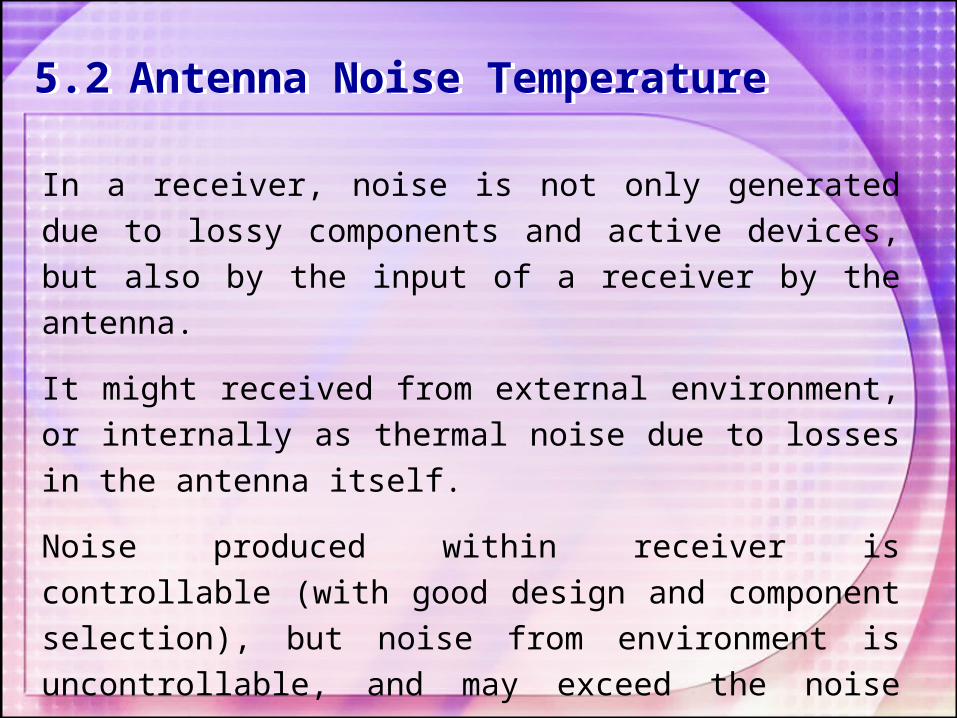
In a receiver, noise is not only generated due to lossy components and active devices, but also by the input of a receiver by the antenna.

It might received from external environment, or internally as thermal noise due to losses in the antenna itself.

Noise produced within receiver is controllable (with good design and component selection), but noise from environment is uncontrollable, and may exceed the noise level of the receiver.

Antenna Noise Temperature (Cont’d..)Antenna Noise Temperature (Cont’d..)

Normally, we have the simple case to measure an

available output noise power N0, given by:

kTBN 0

Illustrating the concept of background temperature. (a) A resistor at temperature T. (b) An antenna in an anechoic chamber at temperature T. (c) An antenna viewing a uniform sky background at temperature T.


Natural and manmade sources of background noise.

The background noise temperature, TB, is the

equivalent temperature of a resistor required to produce the same noise power as the actual environment seen by the antenna


But when the antenna beamwidth is broad enough that different parts of the antenna pattern see different background temperatures, the temperature now is called as effective brightness

temperature, Tb seen by the antenna. This

antenna brightness temperature takes into account the distribution of background temperature, directivity and the power pattern function of the antenna

If the antenna has dissipative loss the radiation

efficiency, erad is less than 1, then the power

available at the terminals of receiver is reduced by

the factor of erad .

This also applies to received noise power, as well as received signal power, so the noise temperature of the antenna will be reduced from the brightness temperature.

Therefore, thermal noise will be generated by resistive losses in the antenna, and will increase the noise temperature of the antenna!!



A receiving antenna connected to a receiver through a lossy transmission

line. An impedance mismatch exists between the antenna and the line.

The relation between the radiation efficiency of the

antenna and the attenuator loss factor is L = 1/erad


The resulting equivalent temperature, TA is called the

antenna noise temperature , with combination of external brightness temperature seen by the antenna and thermal noise generated by the antenna. pradbradp

bA TeTeT

L

L

L

TT

1

1

With Tp is the physical temperature. The antenna noise

temperature is a useful figure for a receive antenna because it characterizes the total noise power delivered by the antenna, to the input of a receiver.


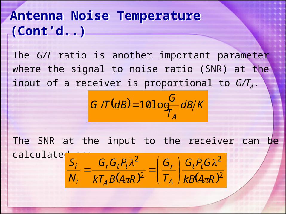
The G/T ratio is another important parameter where the signal to noise ratio (SNR) at the input of a

receiver is proportional to G/TA.

KdBT

GdBTG

A

log10/

The SNR at the input to the receiver can be calculated as:

2

2

2

2

44 RkB

GPG

T

G

RBkT

PGG

N

S tt

A

r

A

ttr

i

i


Where SNR is proportional to G/T of the receive antenna. Only Gr/TA is controllable at the receiver, and others are fixed by the transmitter design and location.

G/T can be maximized by increase the gain of antenna usually minimize reception of noise from hot sources at low elevation angles but higher gain requires larger and more expensive antenna, and high gain may not be desirable for application of omnidirectional coverage!!

Example 2Example 2

The Direct Broadcast System )DBS) operates at 12.2 - 12.7 GHz, with transmit carrier power 120W, transmit antenna gain 34dB, IF Bandwidth 20 MHz, worst case slant angle 300 of satellite to earth of 39,000km. The 18’’ receiving dish antenna has gain of 33.5dB sees an average background brightness temperature Tb = 50K, with receiver LNB noise figure of 1.1dB. Find:

• EIRP of the transmitter

• G/T for the receive antenna and LNB system.

• Received carrier power at the receive antenna terminal

• Carrier to noise ratio (CNR) at the output of LNB

Example 2Example 2


Convert the quantities in dB to numerical values:

34 dB = 2512, 1.1 dB = 1.29, 33.5 dB = 2239Take the operating frequency 12.45 GHz, so wavelength 0.0241m.

So,

dBmWGPEIRP tt 8.541001.32512120 5

Solution to Example 2 (Cont’d..)Solution to Example 2 (Cont’d..)

To find G/T, first find the cascaded noise temperature of the antenna and LNB, with referenced at the input of LNB:

K

TFTTTT bLNBAe

134290129.150

1 0

So then G/T for the antenna and LNB is:

KdBdBTG 2.12134

2239log10/


The received carrier power is from Friis formula:

dBWW

R

GGPP rttr

9.1171063.1

109.34

0241.022391001.3

4

12

272

25

2

2

The CNR at the output of the LNB is:

dB

BGkT

GPCNR

LNBe

LNBr

4.161.44

10201341038.1

1063.1623

12

5.3 Radar5.3 Radar

The operation of monostatic radar (radio detection and ranging) system,

(a) A radar antenna

transmits a signal to

the target.

(b) The target

scatters this signal,

some of which is

received by the radar

antenna.

Radar (Cont’d..)Radar (Cont’d..)

The direction of antenna’s main beam determines the location of the target (azimuth and elevation).

The distance or range to the target corresponds to the time between transmitting and receiving EM pulse.

The speed of target, relative to antenna, can be determined by observing any frequency shift in EM energy (doppler effect).The radar equation,

2

43

2

,41

1

D

RP

P s

rad

rec σs is the radar cross section

Radar (Cont’d..)Radar (Cont’d..)

A more popular expression in terms of an effective area of the radar antenna is :

22441

1e

s

rad

recA

RP

P

The strongest receive power occur when the antenna’s

main beam is pointing at the target, D(θ,φ) = Dmax. The

received power also be detectable over the noise in the

system, so radar will have a minimum detectable power.

37

Example 3Example 3

A radar with minimum detectable power

specified as 1 pW is 1 km distant from a target

with a 1 m2 radar cross section. Operated at 1

GHz the antenna has directivity of 100.

Determine how much power must be radiated to

enable detection of the target.


Solve the radar equation in terms of Prad1 :

max

22

43 1411 D

RPP

srecrad

At 10 GHz, we have λ = 0.3m, then we get:

Wmm

mWPrad 2.2

100

1

3.01

1000410

222

4312

1

Introduction to PropagationIntroduction to Propagation

The propagating wave between transmit and receive antennas in radio communication channel subjects to variety of effects (amplitude, phase or frequency) :-

• Reflection (from the ground or large objects)

• Diffraction (from edges and corners of terrain or buildings)

• Scattering (from foliage or other small objects)

• Attenuation (from rain or the atmosphere)

• Doppler (from moving users)

This list covers the important effects for frequencies above 500 MHz.

For frequencies below, about 100 MHz, other propagation effects can be important:

• ground surface waves

• atmosphere ducting

• ionosphere reflection

Generally, propagation effects have the effect of reducing the received signal power, thus limit the usable range or maximum data rate of a wireless system.

Introduction to Propagation (Cont’d)Introduction to Propagation (Cont’d)

5.4 Free Space Propagation 5.4 Free Space Propagation

From Friis equation, the received power decreases

as 1/R2 with distance from the transmitter path

loss only applies to propagation in free space where no reflection, scattering or diffraction along the path between transmitter and receiver.

Practically, the Friis equation can be used if there’s essentially a single line of sight (LOS) path between transmitter and receiver usually implies that at least one of the link antennas has a narrow beamwidth (high gain) e.g. point to point radio links, satellite to satellite links and earth to satellite links.

Free Space Propagation (Cont’d..) Free Space Propagation (Cont’d..)

A point to point radio link with a single line of sight propagation

path

A cellular telephone channel having multiple propagation

paths.

Free Space Propagation (Cont’d..) Free Space Propagation (Cont’d..)

Multipath propagation is particularly likely when the antennas have broad beams (low gain) and in close proximity to the ground or other large reflecting structures i.e. buildings, vehicles or foliage.

May be no LOS path at all!! common situation for cellular phone located in a building or vehicle.

Communication still possible in multipath or even in the absence of LOS path but the total signal voltage received will have varying degrees of destructive or constructive interference due to the variable phase delays that occur at different paths Friis can not be used!

5.5 Ground Reflections5.5 Ground Reflections

Consider an LOS path with a single reflected signal it’s useful for ground reflections, which frequently occur in practice + reflections from building, vehicles etc.

By Snells Law, the incident wave is specularly reflected from the ground, so that angle of incident = angle of reflection.

Ground Reflections (Cont’d..) Ground Reflections (Cont’d..)

The electric field of an arbitrary antenna can be expresses as:

mV , ˆ, ˆ,,0

r

eFFrE

rjk

And with the well known Friis equation, we can write the received voltage due to direct wave as:

44

000 0

2

0

ddd

RjkRjk

d

rttRjkrd

eCe

R

ZGGPeZPV

Rd is path length of direct ray, Z0 is receiver load

impedance


The constant C :

04ZPGGC trt

Assume d>>h1 and d>>h2, so the Rd can be

approximated using Taylor expansion to get:

d

hhdhhdRd 2

2122

122

Similarly for received reflected voltage,r

Rjk

r R

eCV

r0


With reflection coefficient close to -1 due to angles of incidence close to grazing (small θ ), and then combine the direct and reflected voltages, give:

r

Rjk

d

Rjk

rd R

e

R

eCVVV

rd 00

Assume Rr ≈ Rd ≈ d with negligible error because

d>>h1 and d>>h2, it reduces to:

dhhjk

d

RjkRRjk

d

Rjk

eR

eCe

R

eCV

drd

d/2 210

00

0

11


Where the magnitude of last factor path gain factor , F

d

hhkeF dhhjk 210/2 sin21 210

Observe 0 ≤ F ≤ 2, so that the received voltage maybe doubled (power quadrupled) when 2 signals in phase, or reduced to zero if complete destructive interference occurred.


Define the angle ψ as the elevation angle of the receive antenna as seen at the transmitter

d

h2tan

So then the path gain factor can be rewritten as

tan sin2 10hkF

50

Example 4Example 4

The height of cellular telephone transmit

antenna operating at 1800 MHz is 8.33m. If the

distance to the receiver is 1 km, find the

smallest receiver antenna height that will

maximize the receive signal voltage

51


At 1800 MHz, wavelength = 0.1667m. So,

5033.81 mh

The path gain factor has a maximum when the

argument of sin function is π/2, 3π/2..

,

2101000

502 22210

nhh

d

hhk

for

n=0,1,2,..So the min height for

max path gain is,mh 5

10

22

Path Loss for Ground Reflections Path Loss for Ground Reflections

The received signal in the presence of a ground

reflections varies according to the path gain

factor and is not simply a function of separation

distance.Applying Taylor series gives the received voltage

as:

d

Rjk

d

Rjk

R

ehhCk

R

e

d

hhCkV

dd

2210210

00

2

Path Loss for Ground Reflections Path Loss for Ground Reflections

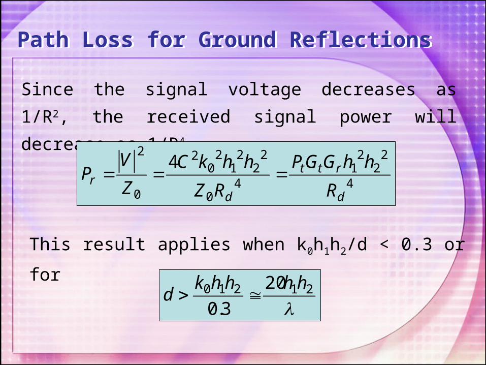
Since the signal voltage decreases as 1/R2, the

received signal power will decrease as 1/R4

4

22

21

40

22

21

20

2

0

24

d

rtt

dr

R

hhGGP

RZ

hhkC

Z

VP

This result applies when k0h1h2/d < 0.3 or for

21210 20

3.0

hhhhkd

Typical Path LossTypical Path Loss

Environment Path Loss Exponent

Free Space 2

Urban 2.7 – 3.5

Shadowed Urban 3 – 5

In Building LOS 1.6 – 1.8

In Building Shadowed 4 – 6

Factory Shadowed 2 – 3

Retail Store 2.2

Office – Soft Partitions 2.4

The resulting path loss can be expressed as 1/Rn ,

where the exponent may vary depends on the

environment.

5.6 Ionosphere Propagation5.6 Ionosphere Propagation

UV light, gamma light and cosmic particles such as electron and proton will ionized gas to generate equal layer labeled as layer D, E and F in ionosphere layer.

EARTH

Virtual height

h

F1

F2

E

D

Ionosphere Propagation (Cont’d..)Ionosphere Propagation (Cont’d..)

The frequency range that can propagates in the ionosphere layer is within 50 kHz to 30 MHz.

Frequencies above 30 MHz can’t get reflected by ionosphere layer where it could get through it. Meanwhile, frequency range between 50 kHz to 30 MHz can get through the lowest layer up to F layer.

Frequencies lower that 50 kHz can propagate lower than the ionosphere layer.


The highest critical wave frequency that incident vertically and the ionosphere able to reflect with is

called critical frequency, fc.

Nfc 9 N = ion density

The maximum frequency that can propagates in the

ionosphere is called maximum usable frequency, fMUF,

determined by critical frequency of F layer and incident angle.

22 4/1sec hdfff cicMUF


The minimum frequency that can propagates in the

ionosphere is called least usable frequency, fLUF,

determined by critical frequency of D layer and incident angle.

Φi is the incident angle of waves in ionosphere, d is

the distance between transmitter and receiver, and h is the virtual height of F layer.


Refraction index, n in the ionosphere can be determined as:

mediuminvelocitywave

vacuuminvelocitywaven

Where its relationship with incident and critical frequency:

2

21

811

f

f

f

Nn c f = incident

frequency

5.7 Troposphere Propagation5.7 Troposphere Propagation

Troposphere layer is the bottom layer in atmosphere from ground to 10km at poles and up to 18km at equatorial. Several mechanisms in troposphere propagation, i.e. direct propagation, refraction, ducting or scattering. Refraction

Three types of refraction: Normal refraction Superfraction Trapping

Troposphere Propagation (Cont’d..)Troposphere Propagation (Cont’d..)

Normal

Superfraction

Trapping


When trapping occurs, wave propagation is concentrated on small area, i.e. same as in waveguide gives optimum signal received, even at far distance away centimeter wave at hot area and wide ocean area, e.g. Mediterranean and Carribean.

Ducting

Earth

Troposphere layer


Troposphere Scattering

It occurs due to inhomogeneous troposphere layer structure at antenna’s cross section path between the transmitter and the receiver.

Earth

Antenna path

This happen because due to discontinuity of dielectric constant in troposphere layer.

The propagation is useful for frequency between 400 MHz to 5 GHz with distance between 300 km to 600 km. However, the received power will be too small. Therefore, high power is needed (1 to 10kW) for transmission.

Scattering is also happen at the bottom of ionosphere with frequency range between 30 MHz to 60 MHz and distance between 1000 km to 2000km with power of 50kW.


5.8 Vegetation Propagation5.8 Vegetation Propagation

Few models being used for estimation of radio wave loss in vegetation area. The first model, where it considers the received wave comes from direct rays and ground reflections.

The E field in free space can be described as :

d

HhEE o

4

Assume that h<<d and H<<d

From previous chapter,

d

GPE tt

o

30

Vegetation Propagation (Cont’d..)Vegetation Propagation (Cont’d..)

The received power after propagated in vegetation area,

22sfer AAAP

φ = flux power at distance dAe = antenna effective areaAf = vegetation lossAs = earth unevenness loss

For flat ground surface, As = 1.


Here,

22

2

2

2

2

4

120/430

120

ftt

tt

Ad

HhGP

d

Hh

d

GP

E

So that,

22

24 fte

t

r Ad

HhGA

P

P


For effective area of aperture antenna,

4

2r

eG

A

So then substitute into previous equation,

2

2

d

HhAGG

P

P ftr

t

r

Where in terms of decibels,

]}[2)(log20)(log40{

][][][][

dBLmhHmd

dBGdBGdBPdBP

f

trtr

Where Lf= 10 log Af


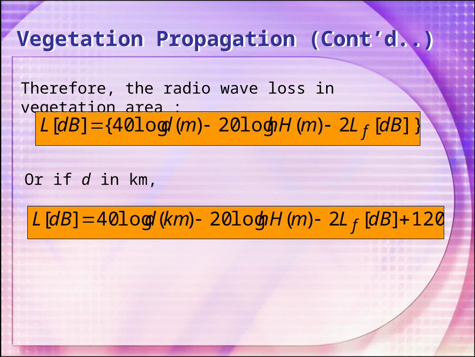
Therefore, the radio wave loss in vegetation area :

]}[2)(log20)(log40{][ dBLmhHmddBL f

Or if d in km,

120][2)(log20)(log40][ dBLmhHkmddBL f


The second model, from ‘Jansky and Bailey’, considers the frequency of radio wave. Consider,

2

4

d

AAGG

P

P sftr

t

r

Replace with λ=c/f and As = 1 for flat surface,

2

4

df

cAGG

P

P ftr

t

r


Where in terms of decibels,

]}[244.32)(log20)(log20{

][][][][

dBLMHzfkmd

dBGdBGdBPdBP

f

trtr

Therefore, the radio wave loss in vegetation area :

][244.32)(log20)(log20][ dBLMHzfkmddBL f

5.9 Urban Propagation5.9 Urban Propagation

Urban area can be described as rough surface area, where it increases the interference of direct waves and reflected waves.

The Lf variable in vegetation loss equation can be

replace with urban loss factor, b. Hence, the loss is:

bmhHmddBL )(log20)(log40][

bHUfb 34.008.140/20 Where,

f = frequency in MHz, U is soil usage factor and Hb is

the height difference between the transmitter and receiver.

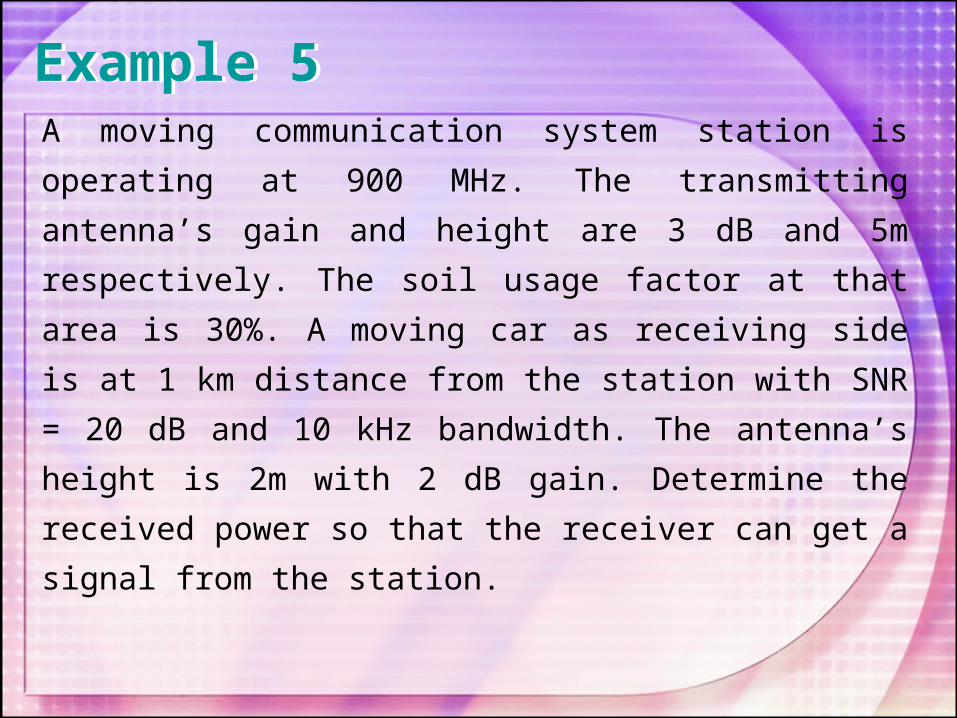
Example 5Example 5

A moving communication system station is operating

at 900 MHz. The transmitting antenna’s gain and

height are 3 dB and 5m respectively. The soil usage

factor at that area is 30%. A moving car as receiving

side is at 1 km distance from the station with SNR =

20 dB and 10 kHz bandwidth. The antenna’s height is

2m with 2 dB gain. Determine the received power so

that the receiver can get a signal from the station.


Substitute into the urban loss factor equation,

844.43334.03.008.140/90020

34.008.140/20

bHUfb

So that,

dBdBL 844.142844.4352log201000log40][

The received power must meet this :

rtRT GGLNNSdBP /][

Where,


NR = kTB = 10 log (1.38x10–23 x 290 x 10 x 103)

= –164

dBdBPT 156.523844.14216420][

Finally,

Or,

WattPT 305.0

AttenuationAttenuation

Attenuation decrease in signal power due to losses in the propagation path.

Material Frequency Loss, dB

Concrete Block Wall

1300 MHz 13

Sheetrock 2 x 3/8” 9.6 GHz 2

Plywood 2 x 3/4” 9.6 GHz 4

Concrete Wall 1300 MHz 8-15

Chain Link Fence 1300 MHz 5-12

Loss Between Floors

1300 MHz 20-30

Corner in Corridor 1300 MHz 10-15

Wireless Communication

Systems and Propagation

Wireless Communication

Systems and Propagation

End

Wireless Communication systems & Propagation Chapter 5.

Documents

Transcript of Wireless Communication systems & Propagation Chapter 5.