libvolume3.xyzlibvolume3.xyz/.../wirelessmodulationtechniquesandhardwaretutorial… · Wireless and...

Wireless and Satellite Communications Prof. Jae Hong Lee, SNU Chapter 6. Modulation Techniques for Mobile Radio - 1 - 2nd Semester, 2010

Chapter 6 Modulation Techniques for Mobile Radio

Text. [1] T. S. Rappaport, Wireless Communications - Principles and Practice, 2/e. Prentice-Hall, 2002.

6.1 Frequency Modulation vs. Amplitude Modulation (skipped)

6.2 Amplitude Modulation (skipped)

6.3 Angle Modulation (skipped)

6.4 Digital Modulation-an overview (mostly skipped)

6.5 Line Coding (skipped)

6.6 Pulse Shaping Techniques (skipped)

6.7 Geometric Representation of Modulation Signals (skipped)

6.8 Linear Modulation Techniques (Mostly skipped)

6.9 Constant Envelope Modulation partly discussed)

6.10 Combined Linear and Constant Envelope Modulation Techniques (briefly covered)

6.11 Spread Spectrum Modulation Techniques (briefly covered)

6.12 Modulation Performance in Fading and Multipath Channels (mostly skipped)

6.x1 OFDM


6.4 Digital Modulation - an Overview (mostly skipped)

6.4.1 Factors That Influence the Choice of Digital Modulation (briefly covered)

A desirable modulation scheme provides low bit error rates at low received signal-to-noise ratios, performs

well in multipath and fading conditions, occupies a minimum of bandwidth, and is easy and cost-effective to

implement.

As existing modulation schemes do not simultaneously satisfy all of these requirements, tradeoffs are made

when selecting a digital modulation, depending on the demand of the particular application.

The performance of a digital modulation scheme is measured in terms of its power efficiency and

bandwidth efficiency.

The power efficiency (sometimes called energy efficiency) p of a modulation scheme is a measure of the

tradeoff between fidelity and signal power (or energy) and is often defined as the ratio of the signal energy

per bit to noise power spectral density 0

bEN

required at the ㅇㄷmodulator input to achieve a certain

probability of error (for example 510 ).


That is,

50 10

bp

BER

EN

.

The bandwidth efficiency B of a modulation scheme is a measure of the ability to accommodate data

within a limited bandwidth and is often defined as the ratio of the throughput data rate per Hertz in a given

bandwidth.

That is,

BRB

bps/Hz (6.36)

where R is the data rate in bit per second and B is the bandwidth occupied by the modulated RF signal.

The system capacity of a digital modulation system is directly related to the modulation scheme.

Shannon’s channel coding theorem states that maximum possible data rate (called channel capacity) is

limited by the noise in the channel for an arbitrary small probability of error for AWGN channels [Shannon,

1948].


From the Shannon’s channel coding theorem, maximum achievable bandwidth efficiency is upper-bounded

as

, maxBCB

2log 1 SN

(6.37)

where C is the channel capacity (in bps), and B is the RF bandwidth and SN

is the signal-to-noise power

ratio.

Besides power efficiency and bandwidth efficiency, there are other factors which also affect the choice of a

digital modulation scheme for a wireless system.

A modulation which is simple to detect is preferred to minimize the cost and complexity of the subscribe

receiver.

A modulation scheme is required to give a good performance under various types of channel impairments

such as Rayleigh and Ricean fading and multipath time dispersion, given a particular demodulator

implementation.


In cellular systems where interference is a major issue, the performance of a modulation scheme in an

interference environment is extremely important.

Sensitivity to detection of timing jitter, which is caused by time-varying channels, is also an important

consideration in choosing a modulation scheme.

Ex. 6.6

DIY.

Ex. 6.7

DIY.


6.4.2 Bandwidth and Power Spectral Density of Digital Signals (briefly covered)

The power spectral density (PSD) of a random signal ( )w t is defined as [Couch, 1993]

2| ( ) |( ) lim Tw T

W fP fT

(6.38)

where the bar stands for an ensemble average and ( )TW f is the Fourier transform of ( )Tw t which is

truncated version of the signal ( )w t , defined as

( ), ,( ) 2 2

0, elsewhere.T

T Tw t tw t

(6.39)

The definition of signal bandwidth varies with context.

The absolute bandwidth of a signal is defined as the range of frequencies over which the signal has a non-

zero power spectral density.

For rectangular baseband pusses, the absolute bandwidth is infinity.

The null-to-null bandwidth is equal to the width of the main spectral lobe.


The half-power bandwidth (also called 3 dB bandwidth) is defined as the interval between frequencies

at which the PSD has dropped to half (or 3 dB) of the peak power.

The FCC adopted the definition of occupied bandwidth as the band which leaves exactly 0.5 % of the

signal power above the upper band limit and exactly 0.5 % of the signal power below the lower band limit so

that 99 % of the signal power is contained within the bandwidth.


6.6 Line Coding (skipped)

Digital baseband signals often use line codes to provide particular spectral characteristics of pulse train.

The most common codes for wireless communication are return-to-zero (RZ), non-return-to-zero (NRZ),

and Manchester codes.

Figure 2.22 [B. Sklar, 2001] shows various commonly used waveforms.


Figure 2.22 Various PCM Waveforms [Sklar, Digital Communications, 2/e., Prentice-Hall, 2001].


The waveform of line codes are shown in Figure 6.14.

(Compare some difference between two figures: Figure 6.14 in the text and Figure 2.22 in Sklars.)


Their power spectral densities are shown in Figure 6.13.


Figure 6.13 Power spectral density of (a) unipolar NRZ.


Figure 6.13 Power spectral density of (b) bipolar RZ.


Figure 6.13 Power spectral density of (c) Manchester NRZ line codes.


6.6 Pulse Shaping Techniques (briefly covered)

When rectangular pulses are passed through a bandlimited channel, the pulses is spread in time, and the pulse

for each symbol smears into the time intervals of succeeding symbols which causes intersymbol interference

(ISI) and increases probability of error at the receiver.

It is desired to have techniques to reduce the modulation bandwidth and suppress out-of-band components,

while reducing intersymbol interference.

Out-of-band radiation in the adjacent channel in a mobile radio system should generally be 40 to 80 dB

below that in the desired passband.

There are various pulse shaping techniques which simultaneously reduce intersymbol interference and the

spectral width of a modulated signal.


6.6.1 Nyquist Criterion for ISI Cancellation (very briefly discussed)

The effective impulse response of a communication system (which consists of the transmitter, channel, and

receiver) is given by

( ) ( ) * ( ) * ( ) * ( )eff c rh t t p t h t h t (6.43)

where ( )p t is the pulse shape of a symbol, ( )ch t is the channel impulse response, and ( )rh t is the receiver

impulse response.

Nyquist found that ISI could be completely nullified if the overall response of a communication system is

designed so that at every sampling instant at the receiver the response due to all symbols except the current (or

‘desired’) symbol is equal to zero.

That is, the impulse response of the overall communication system must satisfy

, 0,( )

0, otherwise,eff s

K nh nT

(6.42)

where sT is the symbol duration, n is an integer, K is a non-zero constant.


Nyquist showed that for zero ISI the transfer function of the overall communication system, ( )effH f , must

satisfy

( ) constanteffk s

kH fT

for all f .

There are two important considerations in selecting a transfer function ( )effH f which satisfy (6.42).

First, ( )effh t should have a fast decay with a small magnitude near the sample values for 0n .

Second, if the channel is ideal (that is, ( ) ( )ch t t ), then it should be possible to realize or closely

approximate shaping filters at both the transmitter and receiver to produce the desired ( )effH f .

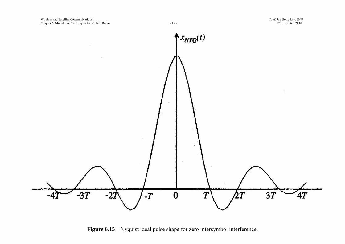
Consider the following impulse response:

sin( )( ) s

eff

s

tTh t t

T

(6.44)

which satisfies the Nyquist condition for ISI cancellation given in (6.42) and shown in Figure 6.15.


Figure 6.15 Nyquist ideal pulse shape for zero intersymbol interference.


If the overall communication system is modeled as a filter with the impulse response of (6.44), the transfer

function of the filter is obtained by taking its Fourier transform, and is given by

1( ) rect( )effs s

fH ff f

(6.45)

which is a rectangular filter with absolute bandwidth 2

sf , where sf is the symbol rate.

While this transfer function satisfies the zero ISI criterion with a minimum of bandwidth, there are practical

difficulties in implementing it, since it corresponds to a non-causal system (that is, ( )effh t is non-zero for

0t ) and is thus difficult to approximate.

Also, the sin tt

pulse has a waveform slope that is 1t

at each zero crossing, and is zero only at exact

multiples of sT , thus any error in the sampling time of zero-crossings will cause significant ISI due to

overlapping from adjacent symbols.

(Note that a slope of 2

1t

or 3

1t

is more desirable to minimize the ISI due to timing jitter in adjacent

samples.)


Nyquist also proved that any filter with a transfer function having a rectangular filter of bandwidth

01

2 s

fT

, convolved with any arbitrary even function ( )Z f with zero magnitude outside the passband of the

rectangular filter, satisfies the zero ISI condition.

That is, the transfer function of the filter which satisfies the zero ISI condition is given by

0

( ) rect( ) ( )efffH f Z ff

(6.46)

where ( ) ( )Z f Z f , and ( ) 0Z f for 01| |

2 s

f fT

.

Expressed in terms of the impulse response, the Nyquist criterion states that any filter with an impulse

response

sin( )( ) ( )s

eff

tTh t z tt

(6.47)

achieves ISI cancellation.

Filters which satisfy the Nyquist criterion are called Nyquist filters (or Nyquist pulse shaping filters) (see

Figure 6.16).


Figure 6.16 Transfer function of a Nyquist pulse-shaping filter at baseband.


Assuming that the distortions introduced in the channel can be completely nullified by using an equalizer

which has a transfer function that is equal to the inverse of the channel response, then the overall transfer

function ( )effH f can be approximated as the product of the transfer functions of the transmitter and receiver

filters.

An effective end-to-end transfer function of ( )effH f is often achieved by using filters with transfer

function ( )effH f at both the transmitter and receiver.

This has the advantage of providing a matched filter response for the system, while at the same time

minimizing the bandwidth and intersymbol interference.


6.6.2 Raised Cosine Rolloff Filter (very briefly covered)

The raised cosine rolloff filter is the most popular pulse shaping filter used in mobile communications which

satisfies the Nyquist criterion.

The transfer function of a raised cosine filter is given by

(1 )1, 0 | | ,2

1 (| | 2 1 ) (1 ) (1 )( ) 1 cos[ ] , | | ,2 2 2 2

(1 )0, | | ,2

s

sRC

s s

s

fT

f TH f fT T

fT

(6.48)

where is the rolloff factor which ranges between 0 and 1.

Figure 6.17 shows the transfer function of the raised cosine filter for various values of the rolloff factor .


Figure 6.17 Magnitude transfer function of a raised cosine filter at baseband.


When 0 , the raised cosine rolloff filter becomes a rectangular filter of minimum bandwidth.

The impulse response of the raised cosine filter is obtained by taking the inverse Fourier transform of the

transfer function, and is given by

2

sin( ) cos( )( ) 41 ( )

2

s sRC

s

t tT Th t tt

T

. (6.49)

Figure 6.18 shows the impulse response of the cosine rolloff filter at baseband for various values of the

rolloff factor .


Figure 6.18 Impulse response of a raised cosine rolloff filter at baseband.


Notice that the impulse response with 0 decays much faster at the zero-crossings (approximately as

3

1t

for st T ) when compared to the rectangular filter ( 0 ).

The rapid time rolloff allows it to be truncated in time with little deviation in performance from theory.

In Figure 6.17 it is shown that as the rolloff factor increases, the bandwidth of the filter also increases,

and the time sidelobe levels decrease in adjacent symbol slots.

This implies that increasing decreases the sensitivity to timing jitter, but increases the occupied

bandwidth.

The symbol rate sR that can be passed through a baseband raised cosine rolloff filter is given by

1s

s

RT

21

B

(6.50)

where B is the absolute filter bandwidth.


For RF systems, the RF passband bandwidth doubles and

1sBR

. (6.51)

The cosine rolloff transfer function can be achieved by using identical ( )RCH f filters at the transmitter

and receiver, while providing a matched filter for optimum performance in a flat-fading channel.

To implement the filter responses, pulse shaping filters can be used either on the baseband data or at the

output of the transmitter.

As a rule, pulse shaping filters are implemented in DSP in baseband.

Because ( )RCh t is noncausal, it must be truncated, and pulse shaping filters are typically implemented for

6 sT about the 0t point for each symbol.

For this reason, digital communication systems which use pulse shaping often store several symbols at a

time inside the modulator, and then clock out a group of symbols by using a look-up table which represents a

discrete-time waveform of the stored symbols.


As an example, assume binary baseband pulses are to be transmitted using a raised cosine rolloff filter with

12

.

If the modulator stores three bits at a time, the there are eight possible waveform states that may be

produced at random for the group.

If 6 sT is used to represent the timespan for each symbol (a symbol is the same as a bit in this case), then

the timespan of the discrete-time waveform will be 14 sT .

Figure 6.19 shows the RF time waveform for the data sequence 1, 0, 1.


Figure 6.19 Raised cosine filtered ( 0.5 ) pulses corresponding to 1, 0, 1 data stream for a BPSK signal.


The optimal bit decision points occur at 4 sT , 5 sT , and 6 sT , and the time dispersive nature of pulse shaping

can be seen.

Notice that the decision points (at 4 sT , 5 sT , 6 sT ) do not always correspond to the maximum values of the

RF waveform.

The spectral efficiency offered by a raised cosine filter only occurs of the exact pulse shape is preserved at

the carrier.

This becomes difficult if nonlinear RF amplifiers are used.

Small distortions in the baseband pulse shape can dramatically change the spectral occupancy of the

transmitted signal.

If not properly controlled, this can cause serious adjacent channel interference in mobile communication

systems.

A dilemma for mobile communication designers is that the reduced bandwidth offered by Nyquist pulse

shaping requires linear amplifiers which are not power efficient.


An obvious solution to this problem would be to develop linear amplifiers which use real-time feedback to

offer more power efficiency, and this is currently an active research thrust for mobile communications.

6.6.3 Gaussian Pulse-Shaping Filter

Unlike Nyquist filters which have zero-crossings at adjacent symbol peaks and a truncated transfer function, a

Gaussian filter has a smooth transfer function with no zero-crossings.

The Gaussian lowpass filter has a transfer function given by

2 2( ) expGH f f (6.52)

where is related to the 3 -dB bandwidth of the baseband Gaussian shaping filter which is given by

ln 22B

0.5887B

. (6.53)

As increases, the spectral occupancy of the Gaussian filter decreases and time dispersion of the output

signal increases.


By taking the inverse Fourier transform of the transfer function, the impulse response of the Gaussian filter

is given by 2

22( ) exp( )Gh t t

. (6.54)

In Figure 6.20 the impulse response of the Gaussian filter is shown for various values of 3 -dB bandwidth-

symbol time product ( SBT ).


The Gaussian filter has a narrow absolute bandwidth (although not as narrow as a raised cosine rolloff filter),

and has sharp cut-off, low overshoot, and pulse area preservation properties which make it very attractive for

use in modulation techniques that use nonlinear RF amplifiers and do not accurately preserve the transmitted

pulse shape.

Since Gaussian pulse-shaping filter does not satisfy the Nyquist criterion for ISI cancellation, reducing the

spectral occupancy results in degradation in performance due to increased ISI.

That is, a tradeoff between the desired RF bandwidth and the irreducible error due to ISI of adjacent

symbols.

Gaussian pulses are used when cost and power efficiency are major factors and the bit error rates due to ISI

are deemed to be lower than what is nominally required.

Ex. 6.8

DIY.

6.7 Geometric Representation of Modulation Signals (skipped)


6.8 Linear Modulation Techniques (mostly skipped)

Digital modulation techniques may be broadly classified as linear or nonlinear.

In linear modulation schemes, the amplitude of the modulated signal ( )s t varies linearly with the

modulating signal ( )m t .

In a linear modulation scheme, the transmitted signal ( )s t is given by [Ziemer, 1992]

( ) Re[ ( )exp( 2 )]cs t Am t j f t

[ ( )cos(2 ) ( )sin(2 )]R c I cA m t f t m t f t (6.65)

where A is amplitude,

cf is the carrier frequency, and

( ) ( ) ( )R Im t m t jm t is complex envelope representation of the modulation signal.

The most popular linear modulations schemes include pulse-shaped QPSK, OQPSK, and / 4 QPSK.


6.8.1 Binary Phase Shift keying (BPSK) (mostly skipped)

The power spectral density (PSD) of a BPSK signal in log scale is shown in Figure 6.22.

In Figure 6.22 it is shown that the null-to-null bandwidth is twice the bit rate, that is,

2null to null bBW R

12bT

.


The probability of bit error for the BPSK is given by

,0

2 bb QPSK

EP QN

(6.74)

where bE is energy per bit and

0N is the double-sided power spectral density of the additive white Gaussian noise (AWGN).

6.8.2 Differential Phase Shift keying (DPSK) (very briefly discussed)

Table 6.1 illustrates the generation of a DPSK signal for a sample sequence km which follows the

relationship 1k k kd m d .


The probability of bit error for the DPSK with non-coherent detection is given by

,0

1 exp( )2

bb DPSK

EPN

(6.75)




6.8.3. Quadrature Phase Shift Keying (QPSK) (very briefly mentioned)

Figure 6.26 shows QPSK signal constellation.


The probability of bit error for the QPSK is given by

,0

2 bb BPSK

EP QN

(6.74)



The bit error probability of QPSK is identical to BPSK, but twice as much data can be sent in the same

bandwidth.

In other words, QPSK provides twice the spectral efficiency with exactly the same energy efficiency in

comparison with BPSK.

The power spectral density of a QPSK signal is given by 2 2

sin ( ) sin ( )2 ( ) ( )

s c s c sQPSK

c s c s

E f f T f f TPf f T f f T

2 2sin 2 ( ) sin 2 ( )

2 ( ) 2 ( )c b c b

bc b c b

f f T f f TEf f T f f T

(6.80)

where bT and sT are bit duration and symbol duration, respectively, and

bE and sE are bit energy and symbol energy, respectively.


The power spectral density (PSD) of a QPSK signal is shown in Figure 6.27.

In Figure 6.27 it is shown that the null-to-null bandwidth is equal to the bit rate, that is,

null to null bBW R

1

bT

which is half that of the BPSK signal.


6.8.4. Quadrature Transmission and Detection Techniques (very briefly mentioned)

Figure 6.28 shows a block diagram of a typical QPSK modulator.


6.8.5 Offset QPSK (OQPSK) (briefly covered)

The amplitude of a QPSK signal is ideally constant.

However, when QPSK signals are pulse shaped to reduce the spectral sidelobes, the waveform no longer has

a constant envelope and the occasional phase shift of 180o can cause the signal envelope to pass through zero

for just an instant.

A signal is sometimes hardlimited to remove any fluctuations in its envelope.

Hardlimiting or nonlinear amplification of the zero-crossings brings back the filtered spectral sidelobes

which interfere adjacent channels, since the fidelity of the signal at small voltage levels is lost in transmission.

To prevent the regeneration of spectral sidelobes and spectral widening, QPSK signals must be amplified

using highly linear amplifiers which are expensive and less efficient.

While the bit transitions of the even and odd bit streams, ( )Im t and ( )Qm t , occur at the same time instants

in QPSK signaling, the even and odd bit streams, ( )Im t and ( )Qm t , are offset in their relative alignment by

one bit period (i.e., half symbol period) in offset QPSK (OQPSK or staggered QPSK (SQPSK)) signaling.


An example of the OQPSK signal is shown in Figure 6.30.


While the phase transition occurs once every 2s bT T with 0o , 90o , 180o , or 270o in QPSK, the phase

transition occurs once every bT with 0o , 90o , or 270o (or 90o ) in OQPSK.

By having phase transition more frequently, the OQPSK signaling eliminates 180o phase transitions.

Since 180o phase transitions are eliminated, bandlimiting (i.e., pulse shaping) does not cause the signal

envelope to go to zero.

Hence, the hardlimiting or nonlinear amplification of OQPSK signals does not regenerate high frequency

sidelobes as much as in QPSK and spectral occupancy of the former is significantly reduced in comparison

with the latter, while permitting more efficient RF amplification.

As the spectrum of an OQPSK signal is identical to that of a QPSK signal, both signals have the same

bandwidth.

OQPSK retains its bandlimited spectrum even after nonlinear amplification.

Hence, OQPSK is attractive for wireless communication systems where bandwidth efficiency and efficient

nonlinear amplifiers are crucial for low power consumption.


Further, OQPSK has better performance than QPSK in the presence of phase jitter due to noisy reference

signals at the receiver [Chunag, 1987].

6.8.6 / 4 QPSK (briefly covered)

For / 4 shifted QPSK, the maximum phase change is limited to 135o (i.e., 135o or 225o ) as compared

with 180o for QPSK and 90o (i.e., 90o or 270o ) for OQPSK.

Hence the bandlimited / 4 QPSK signal preserves the constant envelope property better than bandlimited

QPSK, but not as much as OQPSK.

/ 4 QPSK is very attractive because it can be noncoherently detected which simplifies receiver design

greatly.

Further, / 4 QPSK has better performance than OQPSK in the presence of multipath spread and fading

[Liu, 1989].


In / 4 QPSK modulator, signaling points of the modulated signal are selected from two QPSK

constellations which are shifted by 4 with respect to each other.

Figure 6.31 shows the two constellations along with the combined constellation where a link between two

signal points indicates possible phase transitions.


.

Figure 6.31 Constellation diagram of a / 4 QPSK signal; (a) possible states for k when 1 / 4k n .


Figure 6.31 Constellation diagram of a / 4 QPSK signal; (b) possible states when 1 / 2k n .


Figure 6.31 Constellation diagram of a / 4 QPSK signal; (c) all possible states.


The following figure shows the transitions of / 4 QPSK signals in constellation.


[R. Peterson, R. Ziemer, and D. Both, Introduction to Spread Spectrum Communications. Prentice-Hall, 1995]


Very often, differentially encoded data are / 4 QPSK modulated to facilitate the implementation of

differential detection or coherent modulation with phase ambiguity in the recovered carrier.

When differentially encoded, / 4 QPSK is called / 4 DQPSK.

/ 4 DQPSK is adopted in the standards such as the USDC (IS-54) and PACS in North America and the

PDC (Pacific Digital Cellular) and PHS in Japan.

6.8.7 / 4 QPSK Transmission Techniques

The block diagram of a / 4 QPSK is shown in Figure 6.22.


In the / 4 QPSK transmitter, taking the two bit streams, ,I km and ,Q km , for ( 1)s skT t k T , the

signal mapper produces the k -th in-phase and quadrature data, kI and kQ .

kI and kQ are determined by their previous output values 1kI and 1kQ as well as the phase of k -th

symbol k .

The phase of k -th symbol k itself is a function of k which is a function of current input bits ,I km and

,Q km , which is given by

1k k k , (6.83)

that is,

1k k k .


The outputs of the signal mapper is given by

cosk kI

1cos( )k k

1 1cos sink k k kI Q (6.81)

and

sink kQ

1sin( )k k

1 1sin cosk k k kI Q . (6.82)

The phase shift k is related to input bits kI and kQ as shown in Table 6.2.


Then, as in a QPSK modulator, the in-phase and quadrature bit streams kI and kQ are separately

modulated by two carriers cos ct and sin ct to produce the / 4 QPSK signal which is given by

/ 4 QPSK ( ) ( )cos ( )sinc cs t I t t Q t t (6.84)

where 1

0

( ) ( )2

Ns

k sk

TI t I p t kT

1

0

cos ( )2

Ns

k sk

Tp t kT

(6.85)

and 1

0

( ) ( )2

Ns

k sk

TQ t Q p t kT

1

0

sin ( )2

Ns

k sk

Tp t kT

(6.86)

where the function ( )p t corresponds to the pulse shape and sT is the symbol period.

Usually both kI and kQ are passed through the raised cosine pulse shaping filters before modulation to

reduce the bandwidth occupancy.

Pulse shaping also reduces the spectral restoration problem which may be significant in fully saturated,

nonlinear amplifiers.


Note that the peak amplitudes of the modulated waveforms ( )I t and ( )Q t can take values of 0 , 1 , 1 ,

12

, and 12

.

As the information in a / 4 QPSK signal is completely contained in the phase difference k of the

carrier between two adjacent symbol (that is, 1k k k ), it is possible to apply noncoherent differential

detection even in the absence of differential encoding.

Ex. 6.9

DIY.


6.8.8 / 4 QPSK Detection Techniques (very briefly covered)

Differential detection is often used to demodulate / 4 QPSK signals due to its easy hardware

implementation.

Differentially detected / 4 QPSK has error performance 3 dB inferior to QPSK in an AWGN channel,

while coherently detected / 4 QPSK has the same error performance as QPSK.

In low bit-rate, fast Rayleigh fading channels, differential detection for / 4 QPSK offers a lower error

floor, since it does not rely on phase synchronization [Feher, 1991].

Various types of detection techniques are used for / 4 QPSK such as baseband differential detection, IF

differential detection, and FM discriminator detection.

Baseband Differential Detection

Figure 6.33 shows the block diagram of a baseband differential detector.


The incoming / 4 QPSK signal is quadrature demodulated using two local oscillator signals having the

same frequency as the carrier at the transmitter, but not necessarily the same phase.

Let 1tan kk

k

QI

denote the phase of the carrier due to the k-th data bit, the outputs from the lowpass

filters in the in-phase and quadrature branches are given by

cos( )k kw (6.87)

and

sin( )k kz , (6.88)

respectively, where the is a phase shift due to noise, propagation delay, and interference.

Assume that the phase changes much slower than k so that the former is essentially a constant.

Taking the output sequences from the LPFs, the differential decoders in the in-phase and quadrature

branches give outputs given by

1 1k k k k kx w w z z (6.89)

and

1 1k k k k ky z w w z , (6.90)

respectively.


The differential detector is implemented using a delay line and two mixers.

By plugging (6.87) and (6.88) into (6.89) and (6.90), respectively, the output of the differential detector is

given by

1 1cos( )cos( ) sin( )sin( )k k k k kx

1cos( )k k (6.91)

and

1 1sin( )cos( ) cos( )sin( )k k k k ky

1sin( )k k . (6.92)

Taking the outputs from the differential decoders, the decision devices in the in-phase and quadrature

branches produce outputs given by

1, 0 ,0, 0,

kI

k

xS

x

(6.93)

and

1, 0 ,0, 0,

kQ

k

yS

y

(6.94)

respectively. (Check this with Table 6.2)


Ensure that the frequency of the local oscillator is the same as the transmitter carrier frequency and it does

not drift.

Any drift in the local oscillator frequency causes a drift in output phase which results in degradation in BER.

Ex. 6.10

DIY.

IF Differential Detector (skipped)

Figure 6.34 shows the block diagram of an IF differential detector.


The IF differential detector avoids the need of a local oscillator by using a delay line and two phase

detectors.

The received signal is downconverted to IF and passes through bandpass filter which is matched to the

transmitted pulse shape so that the carrier phase is preserved and noise power is minimized.

To minimize the effect of ISI and noise the bandwidth of the filters are chosen to be 0.57

sT [Liu 1991].

In each branch the received IF signal is differentially decoded using a delay line and two mixers.

The bandwidth of the signal at the output of the differential detector is twice that of the baseband signal at

the transmitter end, as symbols duration the former is half of that of the latter.


FM Discriminator (skipped)

Figure 6.35 shows the block diagram of an FM discriminator detector for / 4 QPSK.


The received signal passes through the bandpass filter matched to the transmitted pulse shape and then

hardlimited to remove any envelope fluctuations.

The FM discriminator extracts the instantaneous frequency deviation of the received signal.

The instantaneous frequency deviation is integrated over each symbol period to give the phase difference

between sampling instants.

Phase difference can be detected using a modulo- 2 phase detector.


6.9 Constant Envelope Modulation

Constant envelope modulation is nonlinear modulation where the amplitude of the carrier is constant

regardless of the variation in the modulating signal.

Constant envelope modulations have advantages as follows [Young, 1979].

Power efficient Class C amplifiers can be used without causing degradation in the bandwidth occupancy of

the transmitted signal.

Low out-of-band radiation can be achieved to the order of 60 to 70 dB.

Limiter-discriminator detection can be used which simplifies receiver design and provides high immunity

against FM noise and signal fluctuation due to Rayleigh fading.

Constant envelope modulations have disadvantages as follows.

They occupy a larger bandwidth than linear modulation schemes.


Hence, in applications where bandwidth efficiency is more important than power efficiency, constant

envelope modulation is not suitable.

BFSK, MSK and GMSK are considered, as examples of constant envelope modulations.

6.9.1 Binary Frequency Shift Keying (BFSK) (skipped)

A binary frequency shift keying (BFSK) signal has constant envelope and has either a discontinuous phase or

constant phase, depending on how the frequency variations according to data symbols are imparted into the

transmitted waveform.

In general, a BFSK signal is given by

FSK

2( ) cos(2 2 ) , if ( ) 1,( )

2( ) cos(2 2 ) , if ( ) 1(or 0),

bH c

b

bL c

b

Ev t f f t m tT

s tEv t f f t m tT

(6.95)

for 0 bt T , where 2 f is a constant offset from the nominal carrier frequency and ( )m t is the

modulating signal.


For a BFSK signal to be continuous, it is required that ( ) 2b b bfT f T fT n for some integer n .

One method to generate an FSK signal is to switch between two independent oscillators according to

whether the data is 0 or 1.

As the resulted waveform is discontinuous at the switching times, this type of FSK is called discontinuous

FSK.

A discontinuous BFSK signal is given by

1

FSK

2

2( ) cos(2 ), if ( ) 1,( )

2( ) cos(2 ), if ( ) 1 (or 0),

bH H

b

bL L

b

Ev t f t m tT

s tEv t f t m tT

(6.96)

for 0 bt T .

Since the phase discontinuities cause several problems such as spectral spreading and spurious

transmissions, this type of FSK is generally not used in highly regulated wireless systems.

The more common method to generate an FSK signal is to frequency modulate a single carrier oscillator

using the message waveform.


This type of modulation is similar to analog FM generation, except that the modulating signal ( )m t is a

binary waveform.

Hence, the BFSK signal is represented as

2( ) cos[2 ( )]bFSK c

b

Es t f t tT

2 cos 2 2 ( ) .t

bc f

b

E f t k m dT

(6.97)

Even though the modulating signal ( )m t is discontinuous at bit transitions, the phase function ( )t is

proportional to the integral of ( )m t and is continuous.

Spectrum and Bandwidth of BFSK Signals

As the complex envelope of an FSK signal is a nonlinear function of the modulating signal ( )m t , its

evaluation is quite involved and is usually performed using actual time-averaged measurements.

The power spectral density of a binary FSK signal consists of discrete frequency components at cf ,


cf n f , and cf n f , where n is an integer.

It can be shown that the PSD of a continuous phase FSK ultimately falls off as the inverse fourth power of

the frequency offset from cf .

However, if phase discontinuities exist, the PSD falls of as the inverse square of the frequency offset from

cf [Couch 1993].

From (6.95) it can be derived that the minimum frequency spacing which allows two FSK signals to be

coherently orthogonal is 122H L

b

f f fT

.

This allows orthogonal detection [Sklar, Digital Communications: Fundamentals and Applications. Prentice

Hall, 2001].

By Carson’s rule the transmission bandwidth of a BFSK signal is given by

2 2TB f B (6.98)

where B is the bandwidth of the baseband binary signal.

Assuming that the first null-to-null bandwidth, the bandwidth of the baseband of rectangular pulses is given


by B R .

Hence the FSK transmission bandwidth becomes

2( )TB f R . (6.99)

If a raised cosine pulse-shaping filter is used, then the transmission bandwidth reduces to

2 (1 )TB f R (6.100)

where is the rolloff factor of the filter.

Coherent Detection of BFSK

Figure 6.36 shows the block diagram of a coherent FSK receiver.


The probability of error for coherent detection of BFSK (or coherent BFSK) is given by

,0

be FSK

EP QN

. (6.101)


Noncoherent Detection of BFSK

Figure 6.37 shows the block diagram of a noncoherent FSK receiver.


The probability of error for noncoherent detection of BFSK (or noncoherent BFSK) is given by

, ,0

1 1exp2 2

be FSK NC

EPN

. (6.102)


6.9.2 Minimum Shift Keying (MSK) (briefly covered)

Minimum shift keying (MSK) is a type of continuous phase-frequency shift keying (CPFSK) of which peak

frequency deviation is equal to 14

the bit rate.

In other words, MSK is continuous phase FSK (CPFSK) with a modulation index of 0.5 .

The modulation index of continuous phase FSK is similar to the FM modulation, and is defined as

2FSK

b

fkR

where f is the peak RF frequency deviation and bR is the bit rate.

The modulation index of 0.5 corresponds to the minimum frequency spacing which allows two FSK

signals to be coherently orthogonal, that is,

0( ) ( ) 0

T

H Lv t v t dt (6.103)

for two FSK signals ( )Hv t and ( )Lv t .

This allows orthogonal detection.


The name minimum shift keying implies the minimum frequency separation (i.e., bandwidth).

MSK is sometimes referred to as fast FSK, as the frequency spacing used is only half as much as that used

in conventional noncoherent FSK [Xiong, 1994].

MSK is attractive in wireless communication systems, as it is a spectrally efficient modulation.

MSK has properties such as constant envelope, spectral efficiency, good BER performance, and self-

synchronizing capability.

The MSK signal can be regarded as a special form of an OQPSK signal where the baseband rectangular

pulses are replaced by half-sinusoidal pulses [Pasupathy, 1979].

Consider the OQPSK signal with the bit streams offset as shown in Figure 6.30.

The MSK signal for an N -bit stream is given by 1

MSK0

( ) ( ) ( 2 )cos2N

I b ci

S t m t p t iT f t

1

0

( ) ( 2 )sin 2N

Q b b ci

m t p t iT T f t

(6.104)


where the baseband pulse shaping function is given by

cos( ), ,2( )

0, elsewhere,

b bb

t T t TTp t

(6.105)

and ( )Im t and ( )Qm t are the “odd” and “even” bits of the data stream, ( )Im t , ( )Qm t { 1, 1} ,

which are fed into the in-phase and quadrature branches of the modulator at the rate of 2

bR .

Although there are a number of variations of MSK in the literature, all of them are continuous phase FSK

(CPFSK) employing different techniques to achieve spectral efficiency [Sundberg 1986].

The MSK signal can be regarded as a special form of a continuous phase FSK (CPFSK) signal if (6.97) is

rewritten as

2 1( ) cos 2 ( ( ) ( ))4

bMSK c I Q k

b b

ES t f m t m t tT T

(6.106)

where 0, if ( ) 1,

, if ( ) 1.I

kI

m tm t

From (6.106) it is deduced that an MSK signal has a constant envelope.


Phase continuity at bit transition periods is ensured by choosing the carrier frequency cf such that

14c

b

f nT

for some integer n . (Verify it. DIY.)

Comparing (6.106) with (6.97), it is concluded that the MSK signal is a FSK signal with binary frequencies

14c

b

fT

and 14c

b

fT

.

The minimum frequency separation is given by 1 1 1( ) ( )4 4 2c c

b b b

f fT T T

.

Further, from (6.105) it can be shown that the phase of the MSK signal varies linearly during each bit period.


MSK Power Spectrum

(The power spectral density of the bandpass signal ( )w t is given by

1( ) [ ( ) ( )]4s g c g cP f P f f P f f (6.41)

where ( )gP f is the power spectral density of ( )g t which is the baseband complex envelope of ( )w t .)

From (6.41) and (6.105) the normalized power spectral density for MSK is given by 2 2

2 2 2 2 2 2

16 cos2 ( ) 16 cos2 ( )( )2 1 16 1 16

b c cMSK

E f f T f f TP ff T f T

. (6.108)

Figure 6.38 shows the power spectral density for MSK along with QPSK and OQPSK.


In Figure 6.38 it is shown that MSK has lower spectral sidelobes than QPSK and OQPSK.

99 % of the MSK power spectrum is contained within a bandwidth 99%1.2

b

BT

, while for QPSK and

OQPSK, 99 % bandwidth is given by 99%8

b

BT

for QPSK and OQPSK.

The faster rolloff of the MSK spectrum is due to its smoother pulse shaping function.

However, in Figure 6.38 it is shown that the main lobe of MSK is wider than QPSK and OQPSK, and hence

the null-to-null bandwidth - -null to nullB of the former is larger than the latter.

That is, in terms of null-to-null bandwidth, MSK is less spectrally efficient than QPSK and OQPSK.

Bandlimiting a MSK signal to meet required out-of-band specifications does not cause the signal envelope

to go through zero, since there is no abrupt change in phase at bit transition periods.

Since the amplitude of MSK signals is kept constant, it can be amplified using efficient nonlinear amplifiers

without generating undesired spectral sidelobes.


The following figure shows a MSK waveform [R. Ziemer and R. Peterson, Digital Communications and

Spread Spectrum Systems. Macmillan, 1985].


The following figure shows the trellis diagram for the type-I MSK [R. Peterson, R. Ziemer, and D. Borth,

Introduction to Spread Spectrum Communications. Prentice-Hall, 1995].


The continuous phase property makes MSK desirable for highly reactive loads. Also MSK has simple

modulation and synchronization circuits.

MSK Transmitter and Receiver

Figure 6.39 shows the block diagram of an MSK modulator.


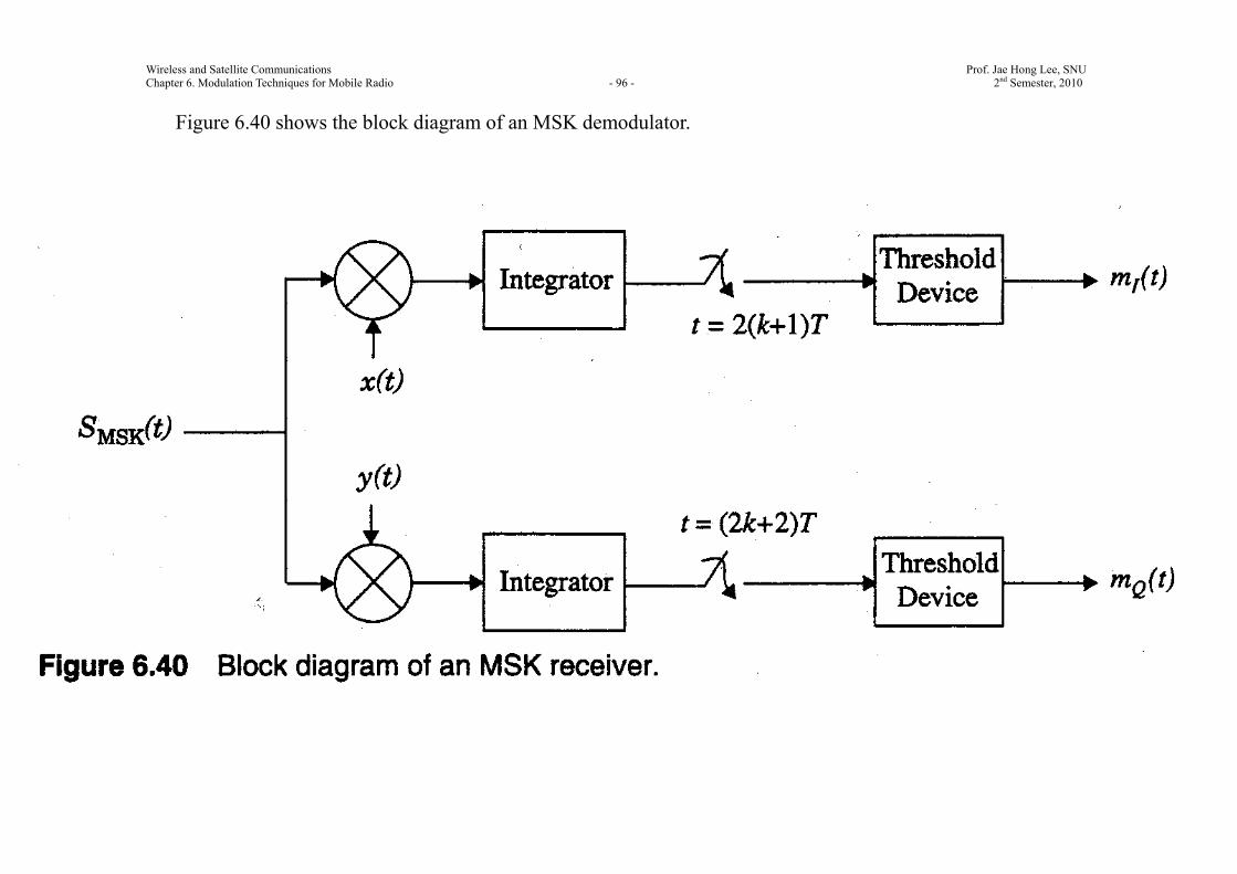
Figure 6.40 shows the block diagram of an MSK demodulator.


6.9.3 Gaussian Minimum Shift Keying (GMSK)

GMSK can be regarded as a variation of MSK.

In GMSK, the sidelobes of the power spectrum are further reduced by passing the modulating NRZ data

waveform through a premodulation Gaussian pulse-shaping filter.

Baseband Gaussian pulse shaping smoothens the phase trajectory of the MSK signal over time and hence

stabilized the instantaneous frequency variations.

By this, the sidelobe levels are reduced considerably in the transmitted spectrum.

The impulse response of the GMSK premodulation filter, which is a Gaussian lowpass filter, is given by 2

22( ) expGh t t

(6.54) (6.109)

where is a parameter related to B which is 3 dB baseband bandwidth of the filter given by

ln22B

0.5887B

. (6.53) (6.111)


Figure 6.22 show the impulse response ( )Gh t of the Gaussian filter.


The has a transfer function of the GMSK premodulation filter, which is a Gaussian lowpass filter, given by 2 2( ) exp( )GH f f . (6.52) (6.110)

As the result of GMSK filtering is completely described by the baseband bandwidth B and the baseband

symbol duration T , it is customary to define GMSK by its B T product.

Figure 6.41 shows power spectrum of the GMSK signal for various values of BT .


Note that the power spectral density of MSK is equivalent to that of GMSK with BT .

In Figure 6.41 it is shown that as the BT product decreases, the sidelobe levels fall off very fast.

For example, the peak of the second lobe is 30 dB below the main lobe for GMSK with 0.5BT , while

the peak of the second lobe is 20 dB below the main lobe for GMSK with BT (that is, MSK).

However, reducing BT increases the irreducible bit error rate produced by the lowpass filter due to ISI.

As to be shown in Section 6.11 mobile radio channels induce an irreducible error rate due to MS velocity.

As long as the GMSK irreducible error rate is less than that produced by the mobile channel,

there is no penalty in using GMSK.

Table 6.3 shows occupied bandwidth containing a given percentage of power in a GMSK signal as a

function of the BT product [Murota, 1981].


While the GMSK spectrum becomes more compact with decreasing BT value, the degradation due to ISI

increases.

It was shown that the BER degradation due to ISI caused by Gaussian filtering is minimum at 0.5887BT ,

where the degradation in the required 0

bEN

is only 0.14 dB from the case of no ISI [Ishizuka 1980].

GMSK Bit Error Rate

The BER of GMSK is a function of BT , since pulse shaping impacts ISI.

The bit error probability of GMSK is given by

0

2 be

EP QN

(6.112a)

where is a constant related to BT by

0.68 for GMSK with 0.25,0.85 for simple MSK ( ).

BTBT

(6.112b)

It is shown that the GMSK with 0.25BT offers BER performance within 1 dB of optimum MSK for

AWGN.


GMSK Transmitter and Receiver

A GMSK signal is generated by passing a NRZ message bit stream through the Gaussian filter having an

impulse response given in (6.109), followed by the FM modulator as shown in Figure 6.42.

The transmitter may also be implemented digitally using a standard /I Q modulator.

A GMSK signal can be detected using orthogonal coherent detectors as shown in Figure 6.43.


GMSK is used in the standards such as the CDPD and DCS-1900 in North America and the GSM and DCS-

1800 in Europe.

Ex. 6.11

DIY.

6.10 Combined Linear and Constant Envelope Modulation Techniques (briefly covered)

Modern modulation techniques exploit the fact that digital baseband data may be sent by varying both the

envelope and phase (or frequency) of an RF carrier.

Because the envelope and phase offer two degrees of freedom, such modulation techniques map baseband

data into four or more possible RF carrier signals.

Such modulation techniques are called M -ary modulation, since they can represent more signals than if

just the amplitude or phase were varied alone.

In an M -ary signaling scheme, two or more bits are grouped together to form symbols and one of M

possible signals, 1 2( ), ( ), , ( )Ms t s t s t is transmitted during each symbol period of duration sT .


Usually, the number of possible signals is 2nM , where n is an integer.

Depending on whether the amplitude, phase, or frequency of the carrier is varied, the modulation scheme is

called M -ary ASK, M -ary PSK, or M -ary FSK.

Modulations which alter both the amplitude and phase of the carrier are the subject of active research.

M -ary signaling with large M is particularly attractive for use in bandlimited channels, but are limited in

their applications due to sensitivity to timing jitter (that is, timing errors increase when signals with smaller

between them in the constellation diagram are used. This results in poorer error performance).

M -ary modulation schemes achieve better bandwidth efficiency at the expense of power efficiency.

For example, an 8 -PSK system requires a bandwidth that is 2log 8 3 times smaller than a BPSK system,

whereas its BER performance is significantly worse than BPSK since signals are packed more closely in the

signal constellation.


6.10.1 M-ary Phase Shift Keying (MPSK or M-PSK) (mostly skipped)

In M -ary PSK, the carrier phase takes on one of M possible values, namely, 21i iM ,

where 1, 2, ,i M .

The modulated waveform can be expressed as

2 2( ) cos(2 ( 1)), 0 , 1, 2, , ,si c s

s

Es t f t i t T i MT M

(6.113)

where 2logs bE M E is the energy per symbol and 2logs bT M T is the symbol period.

(6.113) can be rewritten in quadrature form as

2 2 2 2( ) cos[ ]cos(2 ) sin[( 1) ]sin(2 ), 1, 2, , ,s si c c

s s

E Es t f t i f t i MT M T M

(6.114)

By choosing orthogonal basis signals 12 cos(2 )c

s

t f tT

, and 22 sin(2 )c

s

t f tT

defined over the

interval 0 st T , the M -ary PSK signal set can be expressed as

1 2( ) cos[( 1) ] ( ), sin[( 1) ] ( ) , 1, 2, , ,2 2M PSK s ss t E i t E i t i M

(6.115)


Since there are only two basis signals, the constellation of M -ary PSK is two dimensional.

The M -ary message points are equally spaced on a circle of radius sE centered at the origin.

The constellation diagram of an 8 -ary PSK signal set is illustrated in Figure 6.45.


It is clear from Figure 6.45 that MPSK is a constant envelop signal when no pulse shaping is used.

(6.62) can be used to compute the probability of symbol error for MPSK systems in an AWGN channel.

From the geometry of Figure 6.45, it is easily seen that the distance between adjacent symbols is equal to

2 sin( )sEM .

Hence, the average symbol error probability of an M -ary PSK system is given by

2

0

2 log2 sin( )be

E MP QN M

. (6.116)

Just as in BPSK and QPSK modulation, M -ary PSK modulation is either coherently detected or

differentially encoded for noncoherent differential detection.

The symbol error probability of a differential M -ary PSK system in AWGN channel for 4M is

approximated by [Hay94]

0

42 sin( )2e

EP QN M

. (6.117)


Power Spectra of M-ary PSK

The power spectral density (PSD) of an M -ary PSK signal can be obtained in a manner similar to that

described for BPSK and QPSK signals.

The symbol duration sT of an M -ary PSK signal is related to the bit duration bT by

2logs bT T M . (6.118)

The PSD of the M -ary PSK signal with rectangular pulses is given by

2 2sin sin

2c s c ss

MPSKc s c s

f f T f f TEPf f T f f T

(6.119)

2 2

2 22

2 2

sin log sin loglog2 log log

c b c bbMPSK

c b c b

f f T M f f T ME MPf f T M f f T M

. (6.120)

The PSD of M -ary PSK systems for 8M and 16M are shown in Figure 6.46.


As clearly seen from (6.120) and Figure 6.46, the first null bandwidth of M -ary PSK signals decrease as

M increases while bR is held constant.

Therefore, as the value of M increases, the bandwidth efficiency also increases.

That is, for fixed bR , B increases and B decreases as M is increased.

At the same time, increasing M implies that the constellation is more densely packed, and hence the

power efficiency (noise tolerance) is decreased.

The bandwidth and power efficiency of M -PSK systems using ideal Nyquist pulse shaping in AWGN for

various values of M are listed in Table 6.4.


These values assume no timing jitter or fading, which have a large negative effect on bit error rate as M

increases.

In general, simulation must be used to determine bit error values in actual wireless communication channels,

since interference and multipath can alter the instantaneous phase of an M -PSK signal, thereby creating

errors at the detector.


Also, the particular implementation of the receiver often impacts performance.

In particular, pilot symbols or equalization must be used to exploit M -PSK mobile channels, and this has

not been a popular commercial practice.

6.10.2 M-ary Quadrature Amplitude Modulation (QAM) (mostly skipped)

In M -ary PSK modulation, the amplitude of the transmitted signal was constrained to remain constant,

thereby yielding a circular constellation.

By allowing the amplitude to also vary with the phase, a new modulation scheme called quadrature

amplitude modulation (QAM) is obtained.

Figure 6.47 shows the constellation diagrams of 16 -ary QAM.

The constellation consists of a square lattice of signal points.


The general form of an M -ary QAM signal can be defined as

min min2 2cos 2 sin 2 ,i i c i cs s

E Es t a f t b f tT T

0 , 1, 2, , ,t T i M (6.121)

where minE is the energy of the signal with the lowest amplitude, and

ia and ib are a pair of independent integers chosen according to the location of the particular signal point.

Note that M -ary QAM does not have constant energy per symbol, nor does it have constant distance

between possible symbol states.

It reasons that particular values of is t will be detected with higher probability than others.

If rectangular pulse shapes are assumed, the signal is t may be expanded in terms of a pair of basis

functions defined as

12 cos 2 , 0c s

s

t f t t TT

, (6.122)

22 sin 2 , 0c s

s

t f t t TT

. (6.123)


The coordinates of the i th message point are minia E and minib E , where ,i ia b is an element of the

L L matrix given by

1, 1 3, 1 1, 11, 3 3, 3 1, 3

,

1, 1 3, 1 1, 1

i i

L L L L L LL L L L L L

a b

L L L L L L

(6.124)

where L M .

For example, for a 16 -QAM with signal constellation as shown in Figure 6.47, the L L matrix is given

by

3, 3 1, 3 1, 3 3, 33,1 1,1 1,1 3,1

,3, 1 1, 1 1, 1 3, 13, 3 1, 3 1, 3 3, 3

i ia b

. (6.125)

It can be shown that the average probability of error in an AWGN channel for M -ary QAM, using coherent

detection, can be approximated by [Hay94]

min

0

214 1eEP QNM

. (6.126)


In terms of the average signal energy avE , this can be expressed as [Zie92]

0

314 11av

eEP Q

M NM

. (6.127)

The power spectrum and bandwidth efficiency of QAM modulation is identical to M -ary PSK modulation.

In terms of power efficiency, QAM is superior to M -ary PSK.

Table 6.5 lists the bandwidth and power efficiencies of a QAM signal for various values of M , assuming

optimum raised cosine rolloff filtering in AWGN.


As with M -PSK, the table is optimistic, and actual bit error probabilities for wireless systems must be

determined by simulating the various impairments of the channel and the specific receiver implementation.

Pilot tones or equalization must be used for QAM in mobile systems.


6.10.3 M -ary Frequency Shift Keying (MFSK) and OFDM (partly covered)

In M -ary FSK modulation, the transmitted signals are defined by

2 cos , 0 1,2, , ,si c s

s s

Es t n i t t T i MT T

(6.128)

where / 2c c sf n T for some fixed integer cn .

The M transmitted signals are of equal energy and equal duration, and the signal frequencies are separated

by 12 sT

Hz, making the signals orthogonal to one another.

For coherent M -ary FSK, the optimum receiver consists of a bank of M correlators, or matched filters,

which are tuned to the M distinct carriers.

The average probability of error based on the union bound is given by [Ziemer, 1992]

2

0

log1 be

E MP M QN

. (6.129)

For noncoherent detection using matched filters followed by envelop detectors, the average probability of

error is given by [Ziemer, 1992]


11

1 0

11exp

1 1

kMs

ek

M kEPkk k N

. (6.130)

Using only the leading terms of the binomial expansion, the probability of error can be bounded as

0

1exp2 2

se

M EPN

. (6.131)

The channel bandwidth of a coherent M -ary FSK signal may be defined as [Ziemer, 1992]

2

32logbR M

BM

(6.132)

and that of a noncoherent MFSK may be defined as

22logbR MB

M . (6.133)

This implies that the bandwidth efficiency of an M -ary FSK signal decreases with increasing M .

Therefore, unlike M -PSK signals, M -FSK signals are bandwidth inefficient.

However, since all the M signals are orthogonal, there is no crowding in the signal space, and hence the

power efficiency increase with M .


Furthermore, M -ary FSK can be amplified using nonlinear amplifiers with no performance degradation.

Table 6.6 provides a listing of bandwidth and power efficiency of M -FSK signals for various values of M .

The orthogonality characteristic of MFSK has led to explore orthogonal frequency division multiplexing

(OFDM) as a means of providing power efficient signaling for a large number of users on the same channel.

Each frequency in (6.128) is modulated with binary data (on/off) to provide a number of parallel carriers

each containing a portion of user data.


The radio technologies considered in some standards for wireless communications are shown in the

following table.

Table 6.x. Radio technology, carrier frequency, and maximum rate of some wireless standards.

3GPP LTE IEEE 802.16e

(Mobile WiMAX)WiBro IEEE 802.11n

Radio

technology

DL: OFDMA

UL: SC-FDMA* SOFDMA** OFDMA OFDM

Carrier

frequency 700 MHz – 2.6 GHz 2-11 GHz 2.3 GHz 2.4 / 5 GHz

Maximum

rate

DL: 100 Mbps

UL: 50 Mbps

DL: 128 Mbps

UL: 56 Mbps

DL: 3 Mbps

UL: 1 Mbps

288.9 Mbps (20 MHz channel)

600 Mbps (40 MHz channel)

* SC-FDMA: single carrier FDMA

** SOFDMA: scalable OFDMA


6.11 Spread-Spectrum Modulation Techniques (briefly covered)

Since bandwidth is a limited resource, one of the primary design objectives of all the modulation schemes

dealt so far is to minimize the required transmission bandwidth.

On the other hand, spread spectrum techniques employ a transmission bandwidth which is several orders of

magnitude greater than the minimum required signal bandwidth.

While spread spectrum system is very bandwidth inefficient for a single user, its advantage is that many

users can simultaneously use the same bandwidth without significantly interfering with one another.

In a multi-user wireless environment, spread spectrums system could become very bandwidth efficient if

they are designed with high frequency reuse factor, even though they suffer multiple access interference

(MAI).

Spread spectrum signals are pseudorandom having noise-like properties when compared with digital

information data.


The spreading waveform (spreading signal, signature sequence, spreading sequence, or spreading code) is

controlled by a pseudo-noise (PN) sequence or pseudo-noise code, which is a binary sequence that appears

random but can be reproduced in a deterministic manner by the intended receivers.

Spread-spectrum systems are divided into the following types:

Direct-sequence spread-spectrum (DS-SS)

Frequency-hopped spread-spectrum (FH-SS. Or Frequency-hopping spread-spectrum)

Time-hopped spread-spectrum (TH-SS)

Hybrid spread-spectrum: three types are possible but usually hybrid DS/FH SS.

Spread-spectrum systems have the following advantages.

Easy frequency planning

Since all cells use the same channels and all users share the same spectrum, frequency planning may be

eliminated.

Multiple access interference (MAI) rejection in a CDMA system


Since each user is assigned a unique signature sequence which is approximately orthogonal to the codes of

other users, the receiver can separate the desired signal from others.

Robustness to jamming

When a spread-spectrum signal is jammed by a narrowband interferer (jammer), it can be easily removed

through notch filtering without much loss of information.

Robustness to multipath fading

Wideband signals are affected by selective fading in wireless channels.

Since spread-spectrum signals have uniform energy over a very large bandwidth, only a small portion of its

spectrum in frequency domain will undergo fading at any given time.

Viewed in time domain, it is because the delayed versions of the transmitted PN sequences have poor

correlation with the original PN sequence.

RAKE receiver


A RAKE receiver combines the information obtained from several resolvable multipath components to

improve the system performance.

A RAKE receiver consists of a bank of correlators, each of which correlate to a particular multipath

component of the desired signal.

The correlator outputs are weighted according to their relative strengths and summed to produce the signal

estimate.

6.11.1 Pseudo-Noise (PN) Sequences

A pseudo-noise sequence (PN) or pseudorandom sequence is a binary sequence with an autocorrelation that

resembles the autocorrelation of a random binary sequence. Its autocorrelation roughly resembles that of a

band-limited white noise.

The PN sequence is generated by a feedback shift register shown in Fig 6.48.


Since there are 2 1m non-zero states for an m -stage linear feedback shift register (LFSR), the period of a

PN sequence cannot exceed 2 1m symbols.


A sequence with period 2 1m generated by an m-stage LFSR is called a maximal length (ML) sequence

or m -sequence in short.

6.11.2 Direct-Sequence Spread-Spectrum (DS-SS)

A direct-sequence spread-spectrum system usually adopts BPSK, QPSK, or MSK as a modulation scheme.

A single pulse or symbol of the PN waveform is called a chip.

Figure 6.49 shows a block diagram of a DS-SS system.


Figure 6.49 Block diagram of a DS-SS system with binary phase modulation. (a) transmitter.


In Figure 6.49 a) a code symbol (or chip) from the PN code generator is added in modulo- 2 to a message

symbol (or bit).

The former has shorter duration that the latter.

The transmitted spread spectrum signal is given by

2( ) ( ) ( )cos(2 )sc

s

Es t m t p t f tT

where ( )m t is the data sequence of 1 or 1 , ( )p t is the PN spreading sequence (or code sequence or

signature sequence) of 1 or 1 , f is the carrier frequency, and is the carrier phase.

The received spread spectrum signal is given by

2( ) ( ) ( )cos(2 ) ( )sc

s

Er t m t p t f t n tT

.


Figure 6.49 Block diagram of a DS-SS system with binary phase modulation. (b) receiver.

Figure 6.50 shows the received spectra of the desired spread spectrum signal and the interference at the

output of the receiver wideband filter.


Figure 6.50 Spectra of desired received signal with interference: (a) wideband filter output.


Figure 6.50 Spectra of desired received signal with interference: (b) correlator output after dispreading.


The following figure shows the details on how interference is suppressed in a direct-sequence spread-

spectrum system [R. Peterson, R. Ziemer, and D. Borth, Introduction to Spread Spectrum Communications.

Prentice-Hall, 1995].


Let ( )s bT T and cT denote bit (or symbol) duration and chip duration, respectively,

( )s bR R and cR denote the bit rate and chip rate, respectively, and

B and ssW denote the bandwidths of the baseband signal and spread-spectrum signal, respectively.

Then the interference rejection capability is (approximately) given by ssWB

.

The processing gain of the direct-sequence spread-spectrum system is given by

s

c

TPGT

c

s

RR

2ss

s

WR

ssWB

. (6.136)

Notice that ssW and B are null-to-null bandwidth.


6.11.3 Frequency-Hopped Spread-Spectrum (FH-SS)

Frequency hopping involves a periodic change of transmission frequency.

A frequency hopping signal may be regarded as a sequence of modulated data bursts with time-varying,

pseudorandom carrier frequencies.

Hopping occurs over a frequency band that includes a number of channels.

Each channel is defined as a spectral region with a center frequency and a bandwidth large enough to

include most of the power contained in a narrowband modulation burst (usually M -FSK) having the

corresponding carrier frequency.

The bandwidth of a channel is called instantaneous bandwidth.

The bandwidth of the spectrum over which the hopping occurs is called the total hopping bandwidth.

Figure 6.51 shows a block diagram of a single channel FH-SS system.


Figure 6.51 Block diagram of frequency hopping (FH) system with single channel modulation. a) Transmitter.


Figure 6.51 Block diagram of frequency hopping (FH) system with single channel modulation. b) Receiver.

A frequency-hopped spread-spectrum system usually adopts M -FSK as modulation.


Time duration between hops in frequency domain is called a hop duration or hopping period and its

inverse is called a hopping rate.

If there are one or more symbols during one hop period, then it is called slow frequency-hopping.

If there are more than one hopping in one bit duration, then it is called fast frequency-hopping.

The following two figures illustrate transmitted signals for a) M -ary FSK slow frequency-hopped and

b) fast frequency-hopped spread-spectrum systems [R. Peterson, R. Ziemer, and D. Borth, Introduction to

Spread Spectrum Communications. Prentice-Hall, 1995].


The processing gain of a frequency-hopped spread-spectrum system is given by

ssWPGB

where B and ssW are the instantaneous bandwidth (i.e., the bandwidth of the baseband signal) and the total

hopping bandwidth (i.e., the bandwidth of the spread-spectrum signal), respectively.

6.11.4 Performance of Direct-Sequence Spread-Spectrum (DS-SS)

Consider a CDMA system using the direct-sequence spread-spectrum technique which has K simultaneous

users which is shown in Figure 6.52.


Figure 6.52 A simplified diagram of a DS-SS system with K users.

(a) Model of K users in a CDMA spread spectrum spectrum.


Figure 6.52 A simplified diagram of a DS-SS system with K users. (b) receiver structure for User 1.

Assume that each user has a unique PN sequence with N chips per message bit, that is, b cT NT .

The transmitted signal of the k th user is given by

2( ) ( ) ( )cos(2 )bk k k c k

Es t m t p t f tT

(6.137)

where ( )kp t is the PN sequence, ( )km t is the data sequence, and k is the phase of the k th user.


After the receiver decorrelates the received signal ( )r t with the PN sequence of the user 1, the decision

variable for the i th bit of the user 1 is given by

1

1

(1)1 1 1 1

( 1)

( ) ( )cos 2 ( )b

b

iT

i ci T

Z r t p t f t dt

. (6.138)

For convenience, let 1 0 and 1 0 .

Then, (6.137) can be rewritten as

(1)1

2

K

i kk

Z I I

(6.139)

where 1I is the component of the desired user 1,

kI is the multiple access interference from the k -th user, and

is Gaussian noise with mean zero, and they are given by

1 1 10

( ) ( )cos(2 )bT

cI S t p t f t dt

2b bE T

, when km =1, (6.140)


10

( ) ( )cos(2 )bT

k k k cI S t p t f t dt , (6.143)

and

10

( ) ( )cos(2 )bT

cn t p t f t dt . (6.141)

is a Gaussian random variable with mean zero and variance 2 2[ ]E

0

4bN T

. (6.142)

Assume that each user has a random signature sequence.

Also assume that the signal of each user is transmitted with equal power by perfect power control.

Then, the variance of the interference from the k th user is given by

2

6k

b cI

E T

6b bE TN


of which derivation is given in Appendix E (part E.1) of the text.

Assume that kI , 2, 3, , ,k K are independent (which may not be true in practice).

Then, when K is large, by the central limit theorem, 2

K

kk

I can be approximated to a Gaussian random

variable with variance 2

2k

K

Ik

.

Then, it becomes the problem of detection of message in an AWGN channel.

The probability of bit error is given by

2 2

2

2

k

b b

e K

Ii

E T

P Q

0

2

16 4

b b

b b b

E T

QE T N TK

N


0

11

3 2 b

QK N

N E

. (6.144)

For a single user, i.e., 1K , (6.143) becomes

0

2 be

EP QN

which is the BER for BPSK.

When 0

2 bEN

is large, (6.143) is approximated to

31e

NP QK

(6.145)

which is irreducible error floor due to multiple access interference.

Without careful power control of each MS, one close-in MS may dominate the received signal energy at a

BS which is called a near-far problem, making the Gaussian assumption inaccurate [Pickholtz, 1991].


6.11.5 Performance of Frequency-Hopped Spread-Spectrum

Consider the FH-SS system with K simultaneous users using BFSK modulation.

If two users are not simultaneously utilizing the same frequency slot, the probability of bit error of

noncoherent BFSK is given by

0

1 exp2 2

be

EPN

. (6.146)

Assume that the probability error is 0.5 when two or more users transmit simultaneously in the same

frequency band in a FH-SS system, that is, a “hit” occurs.

Then, the probability of bit error for a FH-SS system is given by

0

1 1exp (1 )2 2 2

be h h

EP p pN

(6.147)

where hp is the probability of a hit.

Suppose that there are M possible hopping channels (called frequency slots).


Assume that all users hop their carrier frequencies synchronously which is called slotted frequency

hopping.

Then, the probability of a hit is given by 111 1 .

K

hpM

For large M, the probability of a hit becomes

11 1 ( 1)hp KM

1KM

. (6.148)

From (6.147) and (6.148), for large M, the probability of bit error is approximated by

0

1 1 1 1exp 12 2 2

be

E K KPN M M

. (6.149)

For a single user system, that is, 1K , (6.149) reduces to (6.146) which is the probability of bit error for

BFSK.


When 0

bEN

is very large, (6.149) is approximated to

0

1 1lim2b

eEN

KPM

(6.150)

which is irreducible error floor due to multiple access interference.

The assumption of slotted frequency hopping is not quite realistic for many FH-SS systems.

Even when synchronization is achieved between individual user clocks, signals from user will not arrive

synchronously due to various propagation delays.

For an asynchronous FH-SS system, the probability of hit is given by [Geraniotis, 1982] 1

1 11 1 1K

hb

pM N

(6.151)

where bN is the number of bits per hop.

From (6.147) and (6.151) the probability of bit error becomes 1 1

0

1 1 1 1 1 1exp 1 1 1 1 12 2

K K

be

b b

EPN M N M N

. (6.152)


The FH-SS system has advantage over the DS-SS system in that it is not susceptible to the near-far problem.

When a ‘hit’ occurs, a burst error occurs. By applying burst error correcting codes such as a Reed-Solomon

code, the probability of bit error can be decreased significantly, even with occasional hits.

6.12 Modulation Performance in Fading and Multipath Channels (mostly skipped)

A wireless channel is characterized by various impairments such as fading, multipath, and Doppler spread.

Although bit error rate (BER) gives a good indication of the performance of a modulation scheme in a

wireless channel, it does not provide any information about outage, i.e., or a complete loss of the signal,

caused by deep fades.

The probability of outage is specified at a specific BER, for example, 310outageP P BER for a voice

channel.


6.12.1 Performance of Digital Modulation in Slow Flat Fading Channels

Since slow, flat fading channels change much slower than the transmitted signal, it is assumed that the

attenuation and phase shift of the signal is constant over at least one symbol interval.

The received signal is given by

( ) ( )exp ( ) ( ) ( ), 0 ,r t t j t s t n t t T (6.153)

where ( )t is the gain of the channel, ( )t is the phase shift of the channel, and ( )n t is an additive white

Gaussian noise.

Depending on whether it is possible to make an accurate estimate of the phase ( )t , coherent or

noncoherent matched filter detection may be employed at the receiver.

The probability of error in a slow flat fading channel is given by

0( ) ( )e eP P X p X dX

(6.154)

where ( )eP X is the probability of error for a modulation scheme at a specific value of signal-to-noise power

ratio (SNR) X , where 2

0

bEXN

, and ( )p x is the pdf of X .


For a Rayleigh fading channel, has a Rayleigh distribution and X has a chi-square distribution with

two degrees of freedom.

The pdf of X is given by

1( ) exp , 0,xp x x (6.155)

where 2

0

bEN

is the average value for the SNR.

The probability of error for coherent BPSK in a slow, flat fading channel is given by

,PSK1 1 (coherent binary PSK)2 1eP

. (6.156)

The probability of error for coherent BFSK in a slow, flat Fading channel is given by

,FSK1 1 (coherent binary FSK)2 2eP

. (6.157)

The probability of error for differential BPSK in a slow, flat Fading channel is given by

,DPSK1 (differential binary PSK)

2(1 )eP

. (6.158)


The probability of error for noncoherent orthogonal BFSK in a slow, flat Rayleigh fading channel is given

by

,NCFSK1 (noncoherent orthogonal binary FSK)

2eP

. (6.159)

Figure 6.53 shows the BERs for various modulation schemes obtained by simulation.


For large value of 0

bEN

(i.e., large values of X ), the probability of error becomes:

,PSK1 (coherent binary PSK)

4eP

(6.160)

,FSK1 (coherent FSK)

2eP

(6.161)

,DPSK1 (differential PSK)

2eP

(6.162)

,NCFSK1 (noncoherent orthogonal binary FSK)eP

. (6.163)

From (6.111a) and (6.153) the probability of error for GMSK is obtained as

,GMSK1 12 1eP

1 (coherent FSK)4

(6.164)

where

0.68, for 0.25,0.85, for .

BTBT

(6.165)


From (6.160) to (6.164) it is shown that the bit error probabilities for all five modulation schemes inversely

proportional to SNR.

According to these results, it is seen that mean SNR of 30 to 60 dB is required to achieve the BER of 310 to 610 which is significantly larger than that required in a nonfading AWGN channel ( 20 to 50 dB

more link SNR is required).

As the poor error performance is due to very deep fades, BER can be significantly decreased by using

techniques such as diversity and/or error control coding to avoid the possibility of deep fades.

Ex. 6.12

DIY.


6.12.2 Digital Modulation in Frequency Selective Mobile Channels

Frequency selective fading due to multipath time delay spread causes intersymbol interference (ISI) which

results in an irreducible BER floor for wireless systems.

Even if a wireless channel is not frequency selective, the time-varying Doppler spread due to motion creates

an irreducible BER floor due to random spectral spreading.

The irreducible error floor in a frequency selective channel is primarily caused by the errors due to the ISI at

sampling instants of the receiver.

ISI occurs when

(a) the main (undelayed) signal component is removed by multipath cancellation,

(b) a nonzero value of the normalized rms delay spread s

dT

, or

(c) the sampling time of the receiver is shifted as a result of delay spread.

Errors in a frequency selective channel is tend to be bursty [Chuang 1987].


For small delay spreads (relative to the symbol duration), the resulting flat fading is the dominant cause of

error bursts.

For large delay spread, timing errors and ISI are the dominant cause.

Figure 6.54 shows the average irreducible BER as a function of d for different unfiltered modulation

schemes with coherent detection.


It is shown that BPSK has the best performance which is because BPSK does not have symbol offset

interference (called cross-rail interference due to multiple rails in the eye diagram).

As both OQPSK and MSK have a 2

sb

T T timing offset between two sequences, the cross-rail interference

is more severe.

Figure 6.55 shows the BER versus rms delay spread normalized to the bit period 'b

dT

.


It is shown that the 4-ary modulations (such as QPSK, OQPSK, and MSK) are more robust to delay spread

than BPSK for a given information throughput.

It is shown that 8 -ary modulation is less resistant than 4 -ary modulation which has made 4 -ary

modulation to be chosen for all 3G (3rd generation) wireless standards: cdma2000 and W-CDMA.

6.12.3 Performance of / 4 DQPSK in Fading and Interference

/ 4 DQPSK is used in the standards such as the USDC and PACS in North America and the PDC and PHS

in Japan.

The performance of / 4 DQPSK has been studied in wireless environment.

The channel was modeled as a frequency selective, 2-ray, Rayleigh fading channel with additive Gaussian

noise and co-channel interference (CCI).

Based on analysis and simulation results , numerical computations are carried out to evaluate the bit error

rate at different multipath delays between the two rays, at different vehicle speeds (i.e., different Doppler

shifts), and various co-channel interference levels.


BER was calculated and analyzed as a function of the following parameters:

Doppler spread mormalized to the symbol rate: D sB T or D

s

BR

Delay of the second multipath , normalized to the symbol duration: T

Ratio of average carrier energy to noise power spectral density in decibels: 0

bEN

dB

Average carrier to interference power ratio in decibles: CI

dB

Average main-path to delayed-path power ratio: CD

dB.

Fung, Thoma, and Rappaport [Fun, 1993] [Rappaport, 1991b] developed a computer simulator called

BERSIM (Bit Error Rate SIMulator) that confirmed the analysis by Liu and Feher [Liu, 1991].


The BERSIM concept, covered under US Patent No. 5,233,628, is shown in Figure 6.56.

Figure 6.56 BERSIM concept. (a) Block diagram of actual digital communication system.


Figure 6.56 BERSIM concept. (b) block diagram of BERSIM using a baseband digital hardware simulator with

software simulation as a driver for real-time BER control (US Patent 5,233,628).

Figure 6.57 shows a plot of the average probability of error of a US digital cellular / 4 DQPSK system as

a function of carrier-to-noise ratio CN

for different co-channel interference levels in a slow Rayleigh flat-

fading channel.


Figure 6.57 BER performance of π/4 DQPSK in a slow flat-fading channel corrupted by CCI and AWGN.

850cf MHz , 24sf ksps raised cosine roll-off factor=0.2, C/I=(1) 20 dB, (2) 30 dB, (3) 40 dB, (4) 50 dB,

(5) infinity [from [Liu91] © IEEE].


Figure 6.58 BER performance versus 0/bE N for / 4 DQPSK in a Raleigh flat-fading channel for various

mobile speeds: 850 , 24c sf MHz f ksps, raised cosine rolloff factor is 0.2, / 100dBC I .

Generated by BERSIM [from [Fun93] © IEEE].


Figure 6.59 BER performance of / 4 DQPSK in a two-ray Rayleigh fading channel, where the time delay , and

the power ratio C/D between the first and second ray are varied. 850MHz, 24c sf f ksps, raised cosine

rolloff rate is 0.2, v=40 km/hr, 120 km/hr 0 100dBbE N . Produces by BERSIM [from [Fun93] © IEEE].


6.x OFDM [Ref. M. Engels, Wireless OFDM Systems: How to make them to work?. Kluwer Academic Press, 2002.]

6.x1.1 OFDM Principle

6.x1.1.1 Multicarrier Modulation

In single carrier modulation, data is sent serially over the channel by modulating one single carrier at a baud

rate of R symbols per second. The data symbol period sT is then 1R

.

In a multipath fading channel, the time dispersion can be significant compared to the symbol period, which

results in intersymbol interference (ISI).

A complex equalizer is then needed to compensate for the channel distortion.

The basic idea of multicarrier modulation was introduced and patented in the mid 60’s by Chang [Chang,

1966]: the available bandwidth W is divided into a number cN of subbands, commonly called subcarriers,


each of width c

WfN

.

The subdivision of the bandwidth is illustrated in Figure 6.x1.1 where arrows represent the different

subcarriers.


Figure 6.x1.1 Subdivision of the bandwidth into cN subbands.


Instead of transmitting the data symbols in a serial way at a baud rate R , a multicarrier transmitter

partitions the data stream into blocks of cN data symbols so that they are transmitted in parallel by

modulating the cN subcarriers.

An OFDM symbol consists of cN data symbols.

The symbol duration in the multicarrier scheme is given by

1s cT N

R .

In its most general form shown in Figure 6.x1.2, the multicarrier signal can be expressed as a set of

modulated carriers: 1

,0

( ) ( )cN

k m k sm k

s t x t mT

(6.x1.1)

where ,k mx is the data symbol modulating the k th subcarrier in the m th signaling interval and

( )k is the waveform for the k th subcarrier.


Figure 6.x1.2 Multicarrier modulation.


The symbol duration can be made long compared to the maximum excess delay of the channel (that is,

max( )cs

NTR

), by choosing cN sufficiently large.

At the same time the bandwidth of the subbands can be made small compared to the coherence bandwidth

of the channel (that is, cc

WBN

), by choosing cN sufficiently large .

Then, each subband experiences flat fading, which reduces equalization to a single complex multiplication

per carrier.

Thus, increasing cN reduces the ISI and simplifies the equalizer into a single multiplication

Note that the number of multiplications is proportional with cN while the rate at which they have to be

calculated is reverse proportional with cN .

However, the performance in time-variant channels is degraded by long symbols.


If the coherence time cT of the channel is small compared to symbol duration sT (that is, cc s

NT TR

),

the channel frequency response changes significantly during the transmission of one symbol and a reliable

detection of the transmitted information becomes impossible.

As a consequence, the coherence time of the channel defines an upper bound for the number of subcarriers,

that is, cc s

NT TR

.

By the condition for time invariance of the channel during a symbol together with the condition for flat

fading within the subbands ( cc

WBN

), a reasonable range for cN can be derived as

c cc

W N RTB . (6.x1.2)


6.x1.1.2 Orthogonal Frequency Division Multiplexing

To assure a high spectral efficiency, the subchannel waveforms must have overlapping transmit spectra.

They need to be orthogonal for enabling simple separation of these overlapping subchannels at the receiver.

Multicarrier modulations that fulfill these conditions are called orthogonal frequency division multiplexing

(OFDM) systems.

A general set of orthogonal waveforms, is given by

1 , [0, ),( )

0, otherwise,

kj tS

sk

e t TTt

(6.x1.3)

with

0 , 0,1, , 1k s ck k N , (6.x1.4)

or

0 , 0,1, , 1k cf f k f k N ,

where 2

kkf

is the subcarrier frequency and 00 2

f

is the lowest frequency used ( 0)k and s is

angular frequency spacing between the adjacent subcarriers.


The frequency spacing between the adjacent subcarriers is given by

2

sf

c

WN

.

Since the waveform ( )k t is restricted to the time window [0, ]sT , the intercarrier spacing must also

satisfy

1

s

fT

c

RN

.

The windowing results in a convolution with sin( )exp( ) ss s

s

fTT j fTfT

in the frequency domain.

As a consequence, the different subbands overlap as shown in Figure 6.x1.3.


Figure 6.x1.3 Spectrum of an OFDM signal.


Although the subchannels overlap, they do not interfere with each other at , 0,1, , 1k cf f k N .

Indeed, they are orthogonal, that is,

*

0( ) ( ) ( )sT

k lt t dt k l . (6.x1.5)

The demodulation of OFDM is based on this orthogonality of the subcariers and consists of a bank of cN

matched filters that implement the relation ( 1) *

, ( ) ( )s

s

m T

k m k smTy s t t mT dt

. (6.x1.6)

A schematic view of such a demodulator is shown in Figure 6.x1.4.


Figure 6.x1.4 OFDM demodulation.


For an OFDM system that consists of oscillators in the transmitter and a bank of matched filters in the

receiver, its implementation is becoming very complex for a large number of subcarriers.

However, as Weinstein and Ebert pointed out [Weinstein, 1971], an IDFT and DFT operation can replace the

baseband modulator and the bank of matched filters, respectively (if cN is a power of two).

In addition to being much cheaper, such implementation does not suffer from the inaccuracies associated

with an analog oscillator bank.


6.x1.1.3 Cyclic Prefix

Passing the signal through a time-dispersive channel causes inter symbol interference (ISI).

In an OFDM system, it also makes the orthogonallity of the subcarriers to be lost, resulting in inter-carrier

interference (ICI).

To overcome these problems, Peled and Ruiz introduced the cyclic prefix (CP) [Peled, 1970].

A cyclic prefix is a copy of the last part of the OFDM symbol that is prepended to the transmitted symbol as

shown in Figure 6.x1.5 and removed at the receiver before the demodulation.


Figure 6.x1.5 Cyclic prefix.


The cyclic prefix should be at least as long as the significant part of the channel impulse response

experienced by the transmitted signal.

This way the benefit of the cyclic prefix is twofold.

First, it avoids ISI because it acts as a guard interval between successive symbols.

Second, it also converts the linear convolution with the channel impulse response into a cyclic convolution.

As a cyclic convolution in the time domain translates into a scalar multiplication in the frequency domain,

the subcarriers remain orthogonal and there is no ICI.

The length of the cyclic prefix should be made longer than the experienced channel impulse response to

avoid ISI as well as ICI.

However, the transmitted energy increases with the length of the cyclic prefix.

The SNR loss due to the insertion of the CP is given by

1010log (1 )cploss

TSNR

T (in dB) (6.x1.7)


where cpT is the length of the cyclic prefix and cp sT T T is the length of the transmitted symbol.

Also the number of symbols per second that are transmitted per Hz of bandwidth, decreases from R to

1 cpTR

T

.

In a digital implementation, cpT is a multiple, cpN , of the basic sample period 1RT

R , that is,

cp cp RT N T .

Because of the loss of SNR and efficiency, the cyclic prefix should not be made longer than strictly

necessary.

When making cpT equal to the length of the impulse response, the relative length of the cyclic prefix cpTT

is

typically small so that the ISI and ICI-free transmission motivates the small SNR loss.


However, when selecting the length of the cyclic prefix, the following issues should also be taken into

consideration:

- Filter responses may add to the overall impulse response that should be compensated for by the guard

interval.

- A part of the guard interval needs to be reserved for synchronization margins.

Not only is the time acquisition never guaranteed to be perfect, the effect of a clock offset between

transmitter and receiver may still significantly increase the deviation.

6.x1.2 OFDM System Model

Figure 6.x1.6 shows the discrete-time baseband equivalent model of an OFDM system which has the DFT and

IDFT operations and the cyclic prefix as basic ingredients.


Figure 6.x1.6 Discrete-time baseband equivalent model of an OFDM system.


In the transmitter, the incoming data stream is grouped in blocks of cN data symbols.

Each of these groups is called an OFDM symbol and can be represented by a vector

0, 1, 1,, , , c

T

m m m N mx x x X where m is the block index.

Next, an IDFT is performed on each data symbol block, and a cyclic prefix of length cpN is added.

The resulting complex baseband discrete time signal of the m th OFDM-symbol is given by 2 ( )1

,0

1 , if {0, 1},( )

0, otherwise,

cpc

c

k n NN jN

k m c cpm kc

x e n N Ns n N

(6.x1.8)

where n is the discrete time index.

The complete time signal ( )s n is given by the concatenation of all OFDM symbols that are transmitted

0

( ) ( ( ))m c cpm

s n s n m N N

. (6.x1.9)

In the received signal is the sum of a linear convolution with the discrete channel impulse response ( )h n

and additive white Gaussian noise (AWGN) ( )n n .


For this, we implicitly assume that the channel fading is slow enough to consider it constant during one

OFDM symbol.

In addition, we assume that the transmitter and receiver are perfectly synchronized.

Based on the fact that the cyclic prefix is sufficiently long to accommodate the channel impulse response, or

( ) 0h n for 0n and 1cpn N , the received signal is given by

1

0( ) ( ) ( ) ( )

cpN

r n h n s n n n

. (6.x1.10)

In the receiver the incoming sequence ( )r n is split into blocks and the cyclic prefix associated with each

block is removed.

This results in a vector ( ( ), ( 1), , ( 1))Tm m m m cr z r z r z N r ,

where ( ) .m c cp cpz m N N N


The received data symbol ,k my is obtained by performing a cN -point DFT on this vector, which is given by

21

,0

( )c

c

knN jN

k m mn

y r z n e

. (6.x1.11)

By substituting ( )r n with (6.x1.10), (6.x1.11) is rewritten as 2 211 1

,0 0 0

( ) ( ) ( )cpc c

c c

kn knNN Nj jN N

k m m cp mn n

y h s N n e n z n e

(6.x1.12)

From (6.x1.8) and (6.x1.12), it becomes 2 211 1

, , ,0 0 0

1( )cpc c

c c

k n knNN N j jN N

k m k m k mn kc

y h x e e nN

(6.x1.13)

where 21

,0

( )c

c

knN jN

k m mn

n n z n e

is the thk sample of the cN -point DFT of ( )mn z n .

Since ( )n n is a white Gaussian noise process, ,k mn is also a white Gaussian noise process (or random

variable).

Because ( ) 0h , for all 1cpN , we can let run from 0 to 1cN instead of 1cpN .


Additional swapping of the two inner sums and reordering yields

2 2 21 1 1

, , ,0 0 0

1 ( )c c c

c c c

k kn knN N N j j jN N N

k m k m k mn kc

IDFT

DFT

y h e x e e nN

. (6.x1.14)

The first part of this expression consists of an IDFT operation nested in a DFT operation.

The inner sum is the thk sample of the cN -point DFT of ( )h , or kh .

Hence (6.x1.14) translates into

, , ,k m k k m k my h x n . (6.x1.15)

(6.x1.15) demonstrates that the received data symbol ,k my on each subcarrier k equals the data symbol

,k mx that was transmitted on that subcarrier, multiplied by the corresponding frequency-domain channel

coefficient kh in addition to the transformed noise contribution ,k mn .

From the received data symbols ,k my the transmitted data symbols ,k mx can be estimated using a single tap

equalizer followed by a slicer.


In the equalizer, the receiver divides each received data symbol ,k my by its corresponding channel

coefficient.

The result of this step is a soft estimate ,k mx .

The slicer rounds this soft estimate towards the nearest symbol in the modulation alphabet, called the hard

estimate ,k mx .

For a more compact notation, a matrix equivalent is often used.

For a single OFDM symbol, it equals

+m m my H x n

=DIAG( ) +m mH x n (6.x1.16)

where denotes the Hadamard (that is, element-wise) product and

DIAG( )H is the diagonal matrix with the elements of H,

0, 1, 1,( , , , )c

Tm m m N my y y y ,

0, 1, 1,( , , , )c

Tm m m N mn n n n , and

0 1 1( , , , )c

TNh h h H = .


Considering M OFDM symbols together, we can express (6.x1.16) into the following matrix form:

Y H X N

DIAG H X + N (6.x1.17)

where 0 1( , , , )MY y y y ,

0 1( , , , ),MX x x x and

0 1( , , , )MN n n n .

libvolume3.xyzlibvolume3.xyz/.../wirelessmodulationtechniquesandhardwaretutorial… · Wireless and...

Documents

Transcript of libvolume3.xyzlibvolume3.xyz/.../wirelessmodulationtechniquesandhardwaretutorial… · Wireless and...