Window-Games between TCP °owsI - Utopia

Window-Games between TCP flowsI

Pavlos S. Efraimidisa,∗, Lazaros Tsavlidisa, George B. Mertziosb

aDepartment of Electrical and Computer Engineering, Democritus University of Thrace,Xanthi, Greece

bDepartment of Computer Science, RWTH Aachen University, Germany

Abstract

We consider network congestion problems between TCP flows and define a newgame, the Window-game, which models the problems of network congestioncaused by the competing flows. Analytical and experimental results show therelevance of the Window-game to real TCP congestion games and provide in-teresting insight into the respective Nash equilibria. Furthermore, we proposea new algorithmic queue mechanism, called Prince, which at congestion makesa scapegoat of the most greedy flow. We provide evidence which shows thatPrince achieves efficient Nash equilibria while requiring only limited computa-tional resources.

Key words: Algorithmic Game Theory, Network Games, Nash Equilibrium

1. Introduction

Algorithmic problems of networks can be studied from a game-theoreticpoint of view. In this context, the flows are considered independent playerswho seek to optimize personal utility functions, such as the goodput. Themechanism of the game is determined by the network infrastructure and thepolicies implemented at regulating network nodes, like routers and switches.The above game theoretic approach has been used for example in [31] and inseveral recent works like [22, 21, 2, 29, 14, 11].

In this work, we consider congestion problems of competing TCP flows,a problem that has been addressed in [19, 2]. We propose a new game, theWindow-game, which models the problem of network congestion caused by thecompeting flows. The novelty of the new model lies in the fact that we focus onthe congestion window, a parameter that is in the core of the network algorithmsof modern TCP flows. The size of the congestion window, to a large degree,controls the speed of transmission of a TCP flow [18].

IA preliminary version of this work has been presented at the Symposium of AlgorithmicGame Theory, SAGT 2008 [8].

∗Corresponding author.Email addresses: [email protected] (Pavlos S. Efraimidis), [email protected]

(Lazaros Tsavlidis), [email protected] (George B. Mertzios)

More precisely, we define the following game, which we call the Window-game, as an abstraction of the TCP congestion problem. The game has a routerand n flows and is played synchronously, in one or more rounds. Every flow is aplayer that in each round selects the size of its congestion window. The router(the mechanism of the game) receives the actions of all the flows and decideshow the capacity is allocated. Based on how much of its requested window hasbeen satisfied, each flow decides on the size of its congestion window for thenext round. The utility of each flow is the capacity that it obtains from therouter in each round minus the cost for lost packets.

The main contributions of this work are three. The first is the definitionof the Window-game, a game-theoretic model for network games between TCPflows. The motivation to address the TCP congestion problem originated fromthe following question, posed in [19, 29]: Of which game or optimization problemis TCP/IP congestion control the Nash equilibrium or optimal solution? TheWindow-game is meant to be a natural model that is simple enough to bestudied from an algorithmic and game-theoretic point of view, while at thesame time it captures essential aspects of the real TCP game. By focusing onthe congestion window, the Window-game is simpler and more abstract thanthe model used in [2], while still being sufficiently realistic to model actualTCP games. The Window-game allows us to address both repeated versions ofthe game that resemble actual TCP games (like the games studied in [2]) andone-shot versions of the game with general (not necessarily AIMD) flows.

The second contribution is the analysis of interesting queue mechanismsfrom a game-theoretic point of view. In particular, the case of DropTail withnon-synchronized packet losses, which we consider the most realistic and inter-esting version of TCP games, has not been addressed before (to the best of ourknowledge). Also new is the analysis of the one-shot versions of the TCP-routergames.

The final contribution is a new queue policy, called Prince, which is simpleand efficient enough to cope with the requirements of real network routers. Weshow that the exemplary punishment of the most greedy flow induces strongincentives for the flows to play in a socially efficient manner. In general, it seemsthat focusing on the most greedy player proves to be a simple and very effectiveway to make selfish players that share a common resource behave responsibly.This claim is further supported by the fact that punishing the highest rate flowhas also been successful in a different network game model [13] where the flowsare Poisson sources. Prince is much simpler than the policy of [13], and it isthe first time the “punish the leader” approach is applied to games with TCPflows.

We provide theoretical evidence and experimental results to support theabove claims.

Outline. The rest of the paper is organized as follows: The Window-gamemodel is described in Section 2. An overview of TCP congestion control conceptsis given in Section 3. The Prince Mechanism along with common router policiesare discussed in Section 4. We consider Window-games where the players areAIMD flows in Section 5 and present the corresponding experimental results in

2

Section 6. Window-games with general, non-AIMD, flows are discussed in Sec-tion 7 (Window-games with complete information) and in Section 8 (Window-games with incomplete information). Finally, a discussion of the results is givenin Section 9.

2. The Window-Game

The Window-game models the interaction between the congestion windowsof competing TCP flows. The main entities of a Window-game are a routerwith capacity C and a set of n ≤ C flows, as depicted in Fig. 1b. The routeruses a queue policy to serve in each round up to C workload. The n flows arethe independent players of the game. Unless otherwise specified, the number nis considered unknown to the players and to the router. The game consists ofone or more rounds. In each round, every player i selects a size wi ≤ C for itscongestion window and submits it to the router. The router collects all requestsand applies the queue policy to allocate the capacity to the flows. The commonresource is the router’s capacity, an abstract concept that corresponds to howmuch load the router can handle in each round. The objective of each player is

(a) The network model of the TCP game. (b) One round of the Window-game.

Figure 1: The Window-game along with the corresponding TCP network model.

to send as many packets as possible. At the same time the player has to avoidpacket losses, as each packet loss induces a cost g ≥ 0 to the player. For gameswith multiple rounds, each packet loss (and each successful packet) causes therespective flow to adjust the size of its congestion window. The adjustment isdetermined by the penalty model and the game strategy of the flow.

Definition 1. One round of the Window-game.Mechanism: A router with capacity C > 0 and a queue policyPlayers: n flows i = 1, . . . , n, where 2 ≤ n ≤ CActions of player i : The window size wi of i, where wi ∈ {1, . . . , C}Utility of player i : u(i) = transmitted(i) - g· dropped(i), where

g: the cost for each dropped packettransmitted(i): number of transmitted packetsdropped(i): number of dropped packets

3

Each round of the game is executed independently; no work is pending at thestart of a round and no work is inherited to a following round.

Network routers and flows process massive streams of network packets inreal time. Therefore, algorithms used by routers and flows may use only limitedcomputational resources like memory and processing power. In particular, it isconsidered unrealistic for network routers to keep detailed statistics on a perflow basis. The queue policy of the router should be stateless or use as littlestate information as possible1.

The Window-game can model not only games between AIMD flows but alsogames between general, not necessarily AIMD, flows. The only requirement isthat that the packet stream generated by each flow can be represented with asequence of window sizes. In this work, we consider the following cases:

Window-Games with AIMD flows. In these games the players are AIMDflows (we provide a short description of AIMD and related concepts inSection 3). Each AIMD flow i selects its parameters (αi, βi) once, forthe whole duration of the game. The utility for each flow is its averagegoodput (number of useful packets that are successfully delivered in eachround) at steady state. This class of Window-games is strongly related tothe game(s) currently played by real TCP flows and exists implicitly inthe analysis of [19, 2].

Window-games with general flows. These are games where the flows canuse arbitrary algorithms to choose their congestion window. Dependingon the number of rounds and on how well each flow is informed about theexistence of other flows, we distinguish the following classes:

• One-shot game with complete information.

• One-shot game with incomplete information with no prior probabil-ities.

• One-shot game with incomplete information with prior probabilities.

• Repeated game with incomplete information.

The action of a general flow is to choose the size of its congestion windowfor each round. In one-shot games, the utility of the flow is the goodputminus the cost for lost packets. In repeated games, the overall utility isthe average utility of all the game rounds.

Assumptions. We make a set of simplifying assumptions similar to the as-sumptions of [2]. The Window-game is symmetric. All flows use the same

1Stateful network architectures are designed to achieve fair bandwidth allocation and highutilization, but need to maintain state, manage buffers, and perform packet scheduling on aper flow basis. Hence, the algorithms used to support these mechanisms are less scalable androbust than those used in stateless routers. The stateless substance of nowadays IP networksallows Internet to scale with both the size of the network and heterogeneous applications andtechnologies [32, 33].

4

network algorithms for loss recovery. All packets of all flows are of the same sizeand have the same Round Trip Time. Packet losses are caused only by networkcongestion.

Solution concept: The solution concept for the Window-games is the Nashequilibrium (NE) and in particular the Symmetric Nash equilibrium (SNE). Agood reason to start with SNE is that the analysis appears to be simpler com-pared to general NE. It is noteworthy, that the both the analytical and theexperimental results show that in many cases there are only symmetric (or al-most symmetric) NE. For each Window-game, we study its SNE and discusshow efficient the network operates at them. In certain cases, we search experi-mentally for general, not necessarily symmetric, NE.

Efficiency and fairness of the NE. In the context of Window-games weconsider a NE efficient if at equilibrium the router capacity is utilized and thepacket losses of the flows are close to zero. We consider a NE fair if all flowsreceive, at least approximately, the same bandwidth.

How realistic is the Window-game? An important difference of Window-games to real TCP/IP games is that Window-games are played in rounds whilereal TCP/IP network games are clocked at the packet level. One round of theWindow-game corresponds to a time-interval roughly equal to the flow’s Round-Trip-Time (RTT), i.e., the time from the submission of a packet P until the cor-responding ACK is received. In this time interval, the flow will receive ACK’sfor all packets that were pending before P. The number of pending packets isdetermined by the window size at the time when packet P where submitted.Therefore, the round-based approach appears to be a natural approximationof the real TCP/IP game. A round-based approach has also been used in theanalysis of [2]. A further difference is that the Window-game model does nottake into account queueing delay. Because of this, the values of the goodput thatare calculated may not always correspond to real goodput values. This, how-ever, is not an obstacle for the applications of the Window-game in this work,since we are mainly interested in the relative goodputs for different strategies ofa TCP flow. Finally, we use the term capacity for the router because we wantto emphasize that this is the amount of work that the router can handle in oneround. The capacity is determined by the bandwidth load that the router canhandle.

In our view, the Window-game fulfils the requirements that we had set: Tocapture the interaction of the competing flows, to indicate when a flow can gainmore goodput by changing its strategy and to characterize the efficiency and thefairness of the NE. Additionally, the analytical and experimental evidence showthat the Window-game is strongly related to the actual TCP/IP congestiongames.

3. Congestion Control in TCP

In this Section, we provide a short description of the basic concepts of TCPand TCP congestion control.

5

TCP: The Transmission Control Protocol (TCP) is one of the core proto-cols of the Internet protocol suite. TCP is a window-based transport protocol;in TCP every flow has an adjustable window, which is called the congestionwindow, and uses it to control its transmission rate [18].

Congestion Window: A TCP flow submits packets to the network andexpects to receive acknowledgments for the packets that reach their destination.The congestion window defines the maximum number of outstanding packetsfor which the flow has not yet received acknowledgements [20]. Essentially,the congestion window represents the sender’s estimate of the amount of trafficthat the network can absorb without becoming congested. The most commonalgorithm to increase or decrease the congestion window of a TCP flow is AIMD.

AIMD: The Additive Increase Multiplicative Decrease (AIMD) algorithm [7]can be considered as a probing procedure designed to find the maximal rate atwhich flows can send packets under current conditions without incurring packetdrops [19]. An AIMD flow i has two parameters αi and βi; upon success, itscongestion window is increased additively by αi (in each round), and upon fail-ure, its congestion window is decreased multiplicatively by a factor βi. Thebasic AIMD algorithm:

wi ={

wi + α, upon successful delivery of all packets of a round,wi · β, in case of packet drop.

AIMD is so far considered to be the optimal choice in the traditional setting ofTCP Reno congestion control and FIFO DropTail routers. If, however, we con-sider the developments like TCP SACK and active queue management, AIMDmay no longer be superior [3].

Packet loss: When congestion occurs at a router, packets are dropped. AnAIMD flow responds to packet loss with a loss-recovery procedure which incurssome cost to the flow and with a decrease of its congestion window. Popularversions of TCP, like TCP Tahoe, TCP-Reno and TCP-SACK, differ in the waythey handle a packet loss.

• TCP Tahoe: A packet loss is indicated when the timeout occurs beforethe corresponding ACK is received. The congestion window will then bereduced to 1 packet and the slow start phase will be initiated. If thesender receives three duplicate ACK (DACK2) for the same packet beforea timeout occurs, the sender first retransmits the packet (fast retransmit)and then reduces its congestion window to 1. This reaction of TCP Tahoecorresponds to the severe reaction to packet loss; even a single packet losscauses the flow to drastically reduce its congestion window.

2When a duplicate ACK is received by a real TCP flow, the flow does not know if it isbecause a TCP segment was lost or simply that a segment was delayed and received outof order at the receiver. If the receiver can re-order segments, it should not be long beforethe receiver sends the latest expected acknowledgement. Typically no more than one or twoduplicate ACKs should be received when simple out of order conditions exist. If however morethan two duplicate ACKs are received by the sender, it is a strong indication that at least onesegment has been lost.

6

• TCP Reno: Has the same mechanism with Tahoe, except that in thecase of 3 DACK it retransmits the packet that the receiver waits for andthen halves its congestion window (fast recovery). In the case of multipledropped packets from the same congestion window, a Reno flow tries mul-tiple fast retransmissions until a timeout occurs and then comes in to slowstart. The reaction of TCP Reno to packet loss is considered a hybridreaction.

• TCP SACK: This variant of TCP is an extension of Reno. SACK hasa selective acknowledgement option that allows receivers to additionallyreport non-sequential data they have received. When coupled with a selec-tive retransmission policy in TCP senders an efficient recovery mechanism,which avoids unnecessary retransmissions, is formed. The reaction of TCPSACK to packet loss is considered a gentle reaction.

Since all loss-recovery schemes incur costs to the flow they can be thoughtof as a penalty on the flows which suspend their normal transmission rate untillost packets are retransmitted.

Penalty Model: We formed a penalty-based model, which is similar to themodel of [19, 2], to define a flow’s behavior when losses occur. Assume that aflow i with current window size wi has lost Li ≥ 1 packets in the last round.Then:

• Gentle penalty (resembles TCP SACK): The flow reduces its window towi = β · wi in the next round.

• Severe penalty (TCP Tahoe): The flow timeouts for τs rounds and thencontinues with a window wi = β · wi.

• Hybrid penalty (TCP Reno): If Li = 1 the flow applies gentle penalty.If Li > 1 a progressive severe penalty is applied. After a timeout ofmin{2 + Li, 15} rounds, the flow restarts with a window equal to wi/Li.This penalty is justified by the experimental results of [9, 27].

4. Router Policies and the Prince Mechanism

The router, and in particular the queue algorithm deployed by the routerto allocate the capacity to the flows, defines the mechanism of the Window-game. We examine the common policies DropTail, RED, MaxMin, CHOKe andCHOKe+. The implementations of the above policies in the Window-game aimto simulate the behavior of the real policies on packet streams. We also examinetwo variants of the proposed Prince policy. Our interest for all policies is on theNE of the corresponding Window-games.

• DropTail: The DropTail policy is the simplest and most common queuediscipline of network routers. With DropTail the packets are served inFIFO order. If the queue is full, incoming packets are dropped. The

7

Window-game adaptation of DropTail, simulates how DropTail would be-have in the real, stream-based case. In each round, if the sum wtotal ofthe requested windows does not exceed the capacity C, the router servesall packets. Otherwise, the router drops a random sample of packets ofsize equal to the overflow, and serves the remaining C packets.

• RED [10]: The Random Early Detection (RED) policy is an active queuemanagement algorithm that may drop packets even before an overflowoccurs. More precisely, at overflow RED behaves like DropTail. However,for queue occupancies between a low threshold minth and a high thresholdmaxth of the queue size, packets are dropped with a positive probabilityp. The Window-game adaptation of RED works as follows: If the sumwtotal of the requested windows is wtotal < minth all packets are served.If wtotal ≥ minth a random sample of packets is selected. The selectedpackets correspond to positions higher then minth in a supposed queue.Each chosen packet is dropped with a probability proportional to therouter’s load. The values minth = 70% and maxth = 100% are used forthe thresholds.

• MaxMin: An allocation of a common resource is MaxMin fair if no sharemay be increased without simultaneously decreasing another share whichis already smaller. Router policies that implement the MaxMin fairnesscriterion achieve fair allocation of the available capacity to the flows.Given a network with its link capacities and a set of flows with theirmaximum possible transmission rates, there is a unique set of flow ratesthat satisfies the max-min conditions. MaxMin Fairness is a stateful, fairqueue policy [5] that conceptually corresponds to applying round-robinfor allocating the capacity. The router offers its packet transmission slotsto its users by polling them in round-robin order. If a flow is offered achance to use a link slot but has no packets ready, then that same slot isoffered to the next flow, until a ready flow is found. In each pass of a link’sround robin, a flow may transmit only one packet [16]. The adaptation ofMaxMin to the Window-game is straightforward.

• CHOKe: CHOKe [28] is a stateless active queue management algorithmthat differentially penalizes misbehaving flows by dropping more of theirpackets. For every packet that arrives at the congested router, CHOKedraws a packet at random from the FIFO buffer and compares it withthe arriving packet. If they both belong to the same flow, then theyare both dropped, else the randomly chosen packet(s) is admitted intothe buffer with a probability that depends on the level of congestion.Packets belonging to a misbehaving flow are both more likely to triggercomparisons and more likely to be chosen for comparison. Therefore,packets of misbehaving flows are dropped more often than packets of well-behaved flows [28]. The Window-game adaptation of CHOKe is similarto the adaption for RED. Every chosen packet that is above the minthreshold, is compared to a packet chosen randomly from the packets that

8

have been admitted until that moment. For the lower threshold, the upperthreshold and the dropping probability we use the same values as for RED.

• CHOKe+: The CHOKE+ policy [2] is a variant of CHOKe that tries toavoid high loss rates and severe under-utilization of the available capacity,when the number of flows is relatively small. For each incoming packet P,the algorithm randomly selects k packets from the queue. Let m denotethe number of packets from the k chosen candidate packets that belongto the same flow as the incoming packet. Let 0 ≤ γ2 ≤ γ1 ≤ 1 be positiveconstants. If m ≥ γ1k, the algorithm drops packet P along with the mmatching candidate packets. Otherwise, a drop probability p is calculatedin an equivalent RED queue. Suppose that P is to be dropped accordingto RED. Now, if γ2k ≤ m < γ1k, the algorithm also drops the m matchingpackets along with P. Otherwise, only packet P is dropped. The Window-game adaption is in the same spirit as the adaptations of CHOKe andRED.

Queue disciplines in use. DropTail is simple and efficient, seems to workreliably in practice and is currently the most widely used queuing discipline atInternet routers. RED is also widely deployed in order to maintain the buffer’sutilization within desired levels. Both DropTail and RED, do not actively punishgreedy flows.

4.1. The Prince MechanismWe propose a new queue policy, called Prince (of Machiavelli), which, at

congestion, drops packets from the flow with the largest congestion window.If the overflow is larger than the window of the most greedy flow, the extrapackets are dropped from the remaining flows with DropTail. If the overflowdoes not exceed the number of packets of the most greedy flow, then flows thatdo not exceed their fair share do not experience packet loss. Hence a greedy flowdoes not plunder the goodput of other flows. The Prince policy is simple anddoes not require state information on a per-flow basis. This makes the policyappropriate for the requirements of real routers. We define a basic version ofPrince that drops packets only in case of overflow and a RED-inspired versionof Prince, called Prince-R, which applies its policy progressively starting froma min threshold minth = 70%.

5. Window-games with AIMD flows

In this Section, we analyze three characteristic Window-game scenarios be-tween AIMD flows with gentle penalty, where the flows can choose the valueof parameter α. Parameter β is fixed3 at its default TCP value β = 1/2. We

3Experiments with parameter β show that in almost all cases selfish flows will use for βa value close to 1. The same conclusion can be extracted from the results in [2]. A simple

9

admit parameter α to take integer values in the range [1, C/2]. In our analysiswe use machinery from [2]. Let us start with the following definitions:

Definition 2. A congestion round of the Window-game is a round in whichthe sum of the requested windows is larger than the capacity of the router. In acongestion round, the router has to drop one or more packets.

Definition 3. A loss round of flow i is a congestion round in which flow iexperiences packet loss.

Assume a set of n AIMD flows where each flow i has parameters (αi, βi). Atsteady state, let Ni denote the window size after a loss round and let τi be thenumber of rounds between two loss rounds of flow i. Let τ be the number ofrounds between two successive congestion rounds of the system. Then, similarto [2], the flow starts after a congestion round with window size Ni and increasesits window size successively to Ni+αi, Ni+2αi, . . . , Ni+αiτi. When the windowsize reaches Ni + αiτi, the flow experiences packet loss and reduces in the nextround its window size to Ni = βi(Ni + αiτi). Hence:

Ni = βi(Ni + αiτi) =12(Ni + αiτi) , (1)

and this givesNi = αiτi . (2)

Assume τi + 1 consecutive rounds, starting immediately after a loss round offlow i. Based on the definition of τi, flow i will not experience packet loss inrounds 1, . . . , τi. However, round τi + 1 will be a loss round for flow i. Thus,the goodput Gi of flow i is:

Gi =1

τi + 1

(Ni + (Ni + αi) + (Ni + 2αi) + . . . + (Ni + αiτi − Li)

),

where Li is the average number of packets that flow i looses at loss rounds. Thisgives:

Gi =32αiτi − 1

τi + 1Li . (3)

In most scenarios we can ignore the last term to get the simplified equation:

Gi =32αiτi . (4)

In the above equations for of AIMD flows we have assumed that the system hasreached a steady state. Based on this assumption we used equations to capture

argument for this behavior is that parameter β is very important when the flow has to quicklyreduce its window size when the network conditions change. The TCP games examined inthis work are rather static: Static bandwidth, static number of flows, static behavior of allflows during a game and hence there is no real reason for a flow to be adaptive.

10

the average behavior of the flows. This approach has been introduced in [2].We will assume that in Window-games with AIMD flows, the flows operate inreasonable conditions, where at minimum

n ≤ C

2, A =

n∑

i=1

αi ≤ C

2, and ∀ flow i, τi ≥ 1 . (5)

We make these assumptions to exclude conditions where Eqs. (1) and (3) becomeinaccurate. The assumptions are reasonable for the scenarios that we consider.

5.1. DropTail router with synchronized packet losses and gentle penalty AIMDflows

The Game: A DropTail router of capacity C serves n gentle penalty TCPflows. The term synchronized packet losses refers to the following simplifyingassumption: At congestion rounds, all flows experience packet loss, that is, everycongestion round is a loss round for all flows.

Using the Window-game model it is easy to show that the selfish flows willtry to over-utilize the common resource (the network) by using a large value fortheir parameter α. The outcome will be a network that is heavily congested.A close analogy is the so-called “Tragedy of the Commons” [17] problem ineconomics where each individual can improve her own position by using more ofa common resource, but the availability of the resource degrades as the numberof greedy users increases.

Since every congestion round is in this game a loss round for all flows, thenumber τi of rounds between two successive loss rounds of any flow i is equalto number τ of rounds between two successive congestion rounds of the system

τ = τ1 = τ2 = . . . = τn . (6)

Let A =n∑

i=1

αi and Ai = A − αi. After each round without packet loss, the

total window size of all flows wtotal =∑n

i=1 wi increases by A. In congestionrounds wtotal exceeds the capacity C of the router, i.e., wtotal > C. The num-ber of excess packets in a congestion round is a random integer in the range1, 2, . . . , A. We will assume that the average excess is L = A/2, i.e., the halfof the increase step. Thus, the total window size wtotal in congestion rounds iswtotal = C +A/2 and the average packet loss for each flow i is Li = αi/2. Aftera congestion round, all flows multiplicatively decrease their congestion window.Using Eq. (2), βi = 1/2 and N =

∑ni=1 Ni we obtain

N =12(C + A/2) . (7)

Using Eq. (1) for all flows and summing up gives:

N =12(N + A · τ) ⇒ τ =

C

2A+

14

. (8)

11

From Eq. (3) we get that for any flow i the goodput Gi is:

Gi(αi) =32αi

(C

2(Ai + αi)+

14

)− αi

(C

Ai + αi+

52

)−1

. (9)

We will show that:

Lemma 4. Gi(αi) in (9) is a strictly increasing function of parameter αi, forαi ≤ C and Ai ≤ C.

Proof. The first derivative of Gi with respect to αi is positive at αi = C, forAi ≤ C. In particular, if the derivative at αi = C is written as a single fraction,its numerator is

15A2i + 57AiC + 14A3

i C + 15C2 + 64A2i C

2 + 3A4i C

2 + 68AiC3

+15A3i C

3 + 18C4 + 24A2i C

4 + 15AiC5 + 3C6,

and its denominator is4(Ai + C)2

(3 + AiC + C2

)2.The second derivative of Gi with respect to αi is always negative. More precisely,the second derivative written can be written as a fraction where the denominatoris strictly positive and the numerator is the sum of the positive terms

12α3i C + 36α2

i AiC + 36αiA2i C + 12A3

i C + 4α3i AiC

2

+12α2i A

2i C

2 + 12αiA3i C

2 + 4A4i C

2,and the negative terms

−81AiC − 81αiAiC2 + 4α3

i AiC2 − 81A2

i C2 − 27α2

i AiC3 − 54αiA

2i C

3

−27A3i C

3 − 3α3i AiC

4 − 9α2i A

2i C

4 − 9αiA3i C

4 − 3A4i C

4.For αi ≤ C, the total sum is always negative, and therefore the second derivativeis always negative. Hence, Gi(αi) is strictly increasing for αi ≤ C. Actually,the result holds even for larger values of Ai up to Ai ≤ 15C, but such valuesare not relevant to the scenarios that we consider. Recall that for AIMD flowswe have assumed the conditions 5.

In normal network conditions, the per flow increase parameters αi and thetotal increase A in each round should be small compared to C. This means thatthe term Li can be neglected in the calculation of the goodput Gi of a flow i andthat in congestion rounds wtotal can be assumed to be wtotal = C. Using theseassumptions in Eqs. (7), (8) and (9), the previous analysis gives the simplifiedexpression

Gi =3αiC

4(Ai + αi), (10)

which is clearly an increasing function of αi.From the above analysis we conclude that in this game, every selfish flow i

will have incentives to increase its parameter αi. The result is that the game willoperate at a very inefficient state, that resembles a Tragedy of the Commonssituation. The above result is not surprising and is in agreement with the resultsin [2].

12

5.2. DropTail router with gentle penalty AIMD flowsWe consider again a Drop-tail router but this time with non-synchronized

packet losses. In this case, at congestion rounds a random set of packets isdropped. The packets to be dropped are randomly selected from the submittedpackets and their number is equal to the packet excess. In each congestionround, a flow may or may not experience packet loss. The expected number ofpackets that it will lose is proportional to its window size. At first glance, thiscase appears to provide better incentives to flows not to behave aggressively.A flow with a smaller congestion window at congestion rounds, has a smallerprobability to experience packet loss, compared to a flow with a larger congestionwindow. However, we will show that this scenario is a Tragedy of the Commonssituation, as well.

This game has not been studied analytically before. The fact that packetlosses are not synchronized makes the analysis harder. We provide an analysisfor a toy case with n = 2 players.

5.2.1. DropTail router with two gentle penalty AIMD flowsThe Game: Assume a router with capacity C and n = 2 flows with para-

meters α1, α2, and β1 = β2 = 1/2. Each flow i can choose the value of itsparameter αi. Simplifications: We assume that at congestion only one flow israndomly selected and the excess is dropped from this flow. Hence only one flowexperiences packet loss in each congestion round. The probability that a flow isselected at a congestion round for dropping the excess packets is proportional tothe flow’s window size. We will also assume that the selected flow has a windowsize at least as large as the excess.

We fix the value α1 of flow 1 and assume that flow 2 chooses a value α2 = zα1,for z > 1. We will show that flow 2 achieves a higher goodput by increasing itsparameter α2. At steady state, we know from Eqs. (2) and (4) that Ni = αiτi

and Gi = 32αiτi − 1

τi+1Li, for i = 1, 2.We can obtain one more expression for the goodput of each flow from a “typ-

ical” congestion round of the router. Let wc,i be the average window size of flowi at congestion rounds. We assume that congestion rounds occur periodically,every τ + 1 rounds. In this case, the average total number of packets requestedby flow i in τ + 1 rounds, where the last round is a congestion round, is

(wc,i − αiτ) + (wc,i − αi(τ − 1)) + . . . + (wc,i − αi) + (wc,i) . (11)

During the above τ + 1 rounds, flow i experiences on average (τ + 1)/(τ1 + 1)loss rounds. At each of its loss rounds, flow i looses on average Li packets.Combining this with Eq. (11) gives that the average goodput of flow i, calculatedfrom an average congestion round and the previous τ rounds, is

Gi = wc,i − 12αiτ − Li

τ1 + 1, (12)

and if we ignore the ÃLi packets that are lost by the flow at loss rounds, thegoodput becomes:

Gi = wc,i − 12αiτ . (13)

13

Step 1: Let wc,i(k) be the window size of flow i at congestion round k and letSi be the number of loss rounds of flow i after a large number K of congestionrounds. Let wc = wc,1 +wc,2 be the mean total number of packets in congestionrounds. Even though wc is a mean value, to simplify the analysis we will assumethat the total number of packets in each congestion round is exactly wc. Then,the probability that flow 1 experiences packet loss in congestion round k iswc,1(k)/wc. We can assume for flow 1 and for each congestion round k a binaryrandom variable X1(k) such that

X1(k) ={

1, flow 1 experiences packet loss in congestion round k,0, otherwise.

Then, the mean value of X1(k) is wc,1(k)/wc. The total number Ψ1 of lossrounds of flow 1 is Ψ1 =

∑k X1(k) and the expected total number of loss

rounds of flow 1 after K congestion rounds is S1 = E[Ψ1] = wc,1Kwc

.We can use an appropriate Hoeffding-Chernoff to show that for large enough

K, the random variable Ψ1 is arbitrary close to S1. Assume a positive constantε, a probability ρ, and a number of rounds K. The following Hoeffding-Chernoffbound is from [15, Page 200, Theorem 2.3].

Theorem 5. Let the random variables Xi(1), Xi(2), . . . , Xi(K) be independent,with 0 ≤ Xi(k) ≤ 1 for k = 1, . . . , K. Let Ψi =

∑Xi(k) and let Si = E[Ψi].

ThenFor any t ≥ 0, P [|Ψi − Si| ≥ Kt] ≤ 2e−2Kt2 .

If K ≥ ln( 12ρ )w2

c

2ε2w2c,1

then by setting t = wc,1Kwc

in Theorem 5 we obtain that

with probability at least ρ, S1 ∈[(1− ε)

wc,1K

wc, (1 + ε)

wc,1L

wc

]. (14)

A sufficiently large number of rounds K can make the constant ε arbitrary smalland the probability ρ arbitrary high. Since we consider the system at steadystate, we can approximate S1 ' wc,1K

wcfor large K. Thus, we will assume

S1 =wc,1K

wc. (15)

Similarly

S2 =wc,2K

wc. (16)

Lety =

wc,2

wc,1. (17)

Then, from Eqs. (15) and (16) we get S2 = y · S1. The frequency fc,i of lossrounds of each flow i = 1, 2 at congestion rounds is fc,i = (τ + 1)/(τi + 1). Itfollows that fc,2/fc,1 = (τ1 + 1)/(τ2 + 1). Additionally, note that fc,2/fc,1 =S2/S1. Thus

y =τ1 + 1τ2 + 1

. (18)

14

Step 2: Since each congestion round is a loss round either for flow 1 or for flow2, the frequency of congestion rounds is equal to the sum of the frequencies ofloss rounds of the two flows:

1τ + 1

=1

τ1 + 1+

1τ2 + 1

. (19)

Using Eqs. (19) and (18) we get

τ =τ1τ2 − 1

τ1 + τ2 + 2=

yτ2 − 1y + 1

=τ1 − y

y + 1. (20)

It followsτ1 = yτ2 + y − 1 and τ2 =

τ1 − y + 1y

. (21)

The number of excess packets in a congestion round is a random integer in therange 1, 2, . . . , (α1 + α2). We will assume that the average excess is the half ofthe mean increase step. This gives that the average total requested window sizewc in congestion rounds is

wc = C +α1 + α2

2. (22)

By the definition of the toy case in each congestion round either flow 1 or flow 2experiences packet loss. We obtain from Eq. (18) that flow 1 experiences packetloss at a congestion round with probability 1/(y+1) and flow 2 with probabilityy/(y + 1). Therefore, for i = 1, 2, the average number Li of packets that flow ilooses at congestion rounds is

L1 =1

y + 1α1 + α2

2and L2 =

y

y + 1α1 + α2

2. (23)

Step 3: Using wc,1 = C+α1+α2

2y+1 and τ = τ1−y

y+1 we can calculate τ1 as follows:

G1 = wc,1 − 12α1τ − 1

τ1+1L1

⇒ 32α1τ1 − 1

τ1+1L1 = C+α1+α2

2y+1 − 1

2α1τ1−yy+1 − 1

τ1+1L1

⇒ 32α1τ1 = C+

α1+α22

y+1 − 12α1

τ1−yy+1 .

(24)

Solving for τ1 gives

τ1 =2C + α1 + zα1 + α1y

3α1y + 4α1. (25)

Step 4: We will obtain one more equation for τ1 by starting this time from thegoodput G2 of flow 2 and then proceeding as in (24):

G2 = wc,2 − 12α2τ − 1

τ2+1L2

⇒ 32α2τ2 − 1

τ2+1L2 = yC+yα1+α2

2y+1 − 1

2α2τ1−yy+1 − 1

τ2+1L2

⇒ 32zα1

τ1−y+1y = 2Cy+α1y+α2y

2(y+1) − 12α2

τ1−yy+1 .

(26)

15

Solving for τ1 gives

τ1 =2Cy2 + α1y

2 + 5zα1y2 − 3zα1

4zα1y + 3zα1. (27)

Step 5: Combining Eqs. (25) and (27) to eliminate τ1 gives the following cubicequation of y:

f(y) = (6C + 15zα1 + 3α1) · y3 + (8C + 16zα1 + 4α1) · y2

−(8Cz + 16zα1 + 4z2α1) · y − (6Cz + 15zα1 + 3z2α1) = 0 .(28)

Lemma 6. For z > 0, Eq. (28) has exactly one positive real solution y(z) andthis solution is a strictly increasing function of z.

Proof. Note that f(0) = −(6Cz + 15zα1 + 3z2α1) < 0 and that f(1 + z) > 0(substituting y = z + 1 and simplifying the expression gives a sum of strictlypositive terms). The derivative of f(y) with respect to y is

f ′(y) = (18C + 9α1 + 45zα1) · y2 + (16C + 8α1 + 32zα1) · y−(8Cz + 16zα1 + 4z2α1) .

(29)

Consider the equationf ′(y) = 0 . (30)

The discriminant of Eq. (30) is

∆ = (16C + 8α1 + 32zα1)2

+4 (18C + 9α1 + 45zα1) (8Cz + 16zα1 + 4z2α1) ,(31)

which is strictly positive for z > 0. Consequently, Eq. (30) has two real solutions

y1,2 =−16C − 8α1 − 32zα1 ±

√∆

2(18C + 9α1 + 45zα1). (32)

From (31) and (32), it is clear that one solution is negative and one is positive.Let y2 be the positive solution of (29). The function f(y) is decreasing in theinterval (0, y2) and increasing in (y2,∞). Since f(0) < 0, it follows that f(y) hasexactly one positive real solution y(z), as a function of z > 0. Since f(y2) < 0,it follows that

y(z) > y2 . (33)

Since, by definition, y(z) is a root of function f(y), after replacing y by y(z)in (28), differentiating f(y(z)) with respect to z, and solving for the derivativey′(z) we obtain

y′(z) =num(z)den(z)

, where:

num(z) = −15α1(y(z))3 − 16α1(y(z))2 + (8C + 8zα1 + 16α1)y(z)+(6C + 15α1 + 6zα1)

den(z) = (18C + 9α1 + 45zα1)(y(z))2 + (16C + 8α1 + 32zα1)y(z)−(8Cz + 16zα1 + 4z2α1)

(34)

16

For the numerator num(z) note that:

f(y(z)) + z · num(z) = 3z2α1 + 4z2α1y(z) + 4α1(y(z))2 + 8C(y(z))2

+3α1(y(z))3 + 6C(y(z))3 > 0 (35)

Since f(y(z)) = 0 and z > 0, it follows that num(z) > 0. For the denominatorden(z) in Eq. (34), note that den(z) = f ′(y(z)). Now, since y(z) > y2 we getthat den(z) is strictly positive. From this we conclude that y′(z) is strictlypositive, for z > 0. This completes the proof.

Since α2 = zα1, Eqs. (4) and (21) imply that:

G2(z) =32α2τ2 =

32zα1

τ1 − y + 1y

(36)

Now we substitute τ1 from Eq. (27) and get:

G2(z) =6Cy + 3α1y + 3zα1y + 3zα1

8y + 6. (37)

Lemma 7. Function G2(z) in (37) is increasing for z > 0.

Proof. Taking into consideration that y is a function of z, the derivative of G2(z)with respect to z is:

G′2(z) =9α1 + 21α1y + 12α1y

2 + 9α1y′ + 3(C − zα1)y′

2(3 + 4y)2. (38)

Since C ≥ zα1 = α2 and y′ > 0, the proof is complete.

In Eq. (36) we can also use the more accurate Eq. (3). In this case, numer-ical evaluations show that G2(z) is still an increasing function of z. However,the analytical expression becomes very complicated. Note that Eqs. (25), (27)and (28) are not influenced if we use the less accurate equation for the goodput,because the term Li is eliminated in Eqs. (24) and (26).

We used the analytical results on a representative game instance with routercapacity C = 100 and n = 2 flows. The calculations have been performed usingMathematica. In particular, we calculated the positive solution of y(z) fromEq. (28). The results are presented graphically in Fig. 2a. The correspondingplots of τ1 and τ2 are given in Fig. 2b.

We used Eq. (3) to calculate the goodputs G1 and G2 of flows 1 and 2,respectively. We also used the less accurate Eq. (4) to calculate G2,approx forflow 2. The results are shown in Fig. 3a. The experimental results for thegoodputs G1 and G2 are presented in Fig. 3b. The graphs show that the resultsof the analytical model are very close to the numerical and the experimentalresults, and confirm that the goodput G2(z) of flow 2 is an increasing functionof z.

The experiments for the toy case with two flows have been conducted witha simple simulator for Window-games with basic AIMD flows, called NetK-nackBasic. The router capacity was C = 100. To avoid or at least reduce

17

10 20 30 40 50

1

2

3

4

5

6

(a) The graph of y as a function of z.

10 20 30 40 50

5

10

15

20

25

30

(b) The graphs of τ1 and τ2 (lower line) asfunctions of z.

Figure 2: Analytical results for y, τ1 and τ2.

0 10 20 30 40 500

20

40

60

80

(a) The analytical results for goodputs G1

(lower line), G2 and G2,approx (dashedline) as functions of z.

0 10 20 30 40 500

20

40

60

80

(b) The experimental results for goodputsG1 (lower plot) and G2 as functions of z.

Figure 3: Analytical and experimental results for goodputs G1 and G2 as func-tions of z.

synchronization effects the capacity varied randomly from C − 1 to C + 1 withan average of C. Parameter α was α1 = 1 for flow 1 and α2 = zα1 for flow 2.Each game lasted for 100000 rounds.

5.3. Prince router with gentle penalty flowsWe now consider the case of a Prince router of capacity C and n flows i =

1, . . . , n with parameters (αi, βi = 1/2). We start with two general propertiesof this game. Assume that the system has reached steady state and that theoverflow in congestion rounds does not exceed the maximum of all windowsmaxi=1,...,n wi.

18

Lemma 8. Let flows i and k be the flows of minimum and maximum goodput,respectively, and let λ = Gk/Gi. Then, it holds λ ≤ 2.

Proof. From Eq. (4) we know that Gi = 32αiτi and that the average window

size of i at its loss rounds is wc,i = 2αiτi. Similarly, Gk = 32αkτk and wc,k =

2αkτk. Note that the congestion window of flow k takes values in the range12wc,k, . . . , wc,k. Flow i has at its congestion rounds the maximum windowamong all flows. Thus wc,i ≥ 1

2wc,k ⇒ αiτi ≥ 12αkτk ⇒ Gi ≥ 1

2Gk ⇒ λ ≤ 2.

Lemma 9. In congestion rounds with total overflow at most maxi=1,...,n wi aflow that does not exceed its fair share C/n, does not lose any packet.

Proof. At congestion,∑n

i=1 wi > C. Clearly, maxi=1,...,n wi > C/n. Thus, aflow i with wi ≤ C/n cannot have the maximum window.

We consider first a toy case with n = 2 flows and then the more general casewith n flows.

5.3.1. Prince router with two gentle penalty AIMD flowsThe Game: Assume a Prince router with capacity C and two flows i = 1, 2

with parameters α1, α2, and β1 = β2 = 1/2. Each flow can choose its parameterα.

We fix α1 and assume that α2 > α1. Then, let α2 = zα1, for z > 1. Atsteady state G1 = 3

2α1τ1 and G2 = 32α2τ2. Assuming λ such that G2 = λG1,

we getzτ2 = λτ1 . (39)

If wc,2 is the average window size of flow 2 at its loss rounds then from Eqs. (1)and (2) we know that wc,2 = 2zα1τ2. Let ws,1 be the average window size offlow 1 in rounds that are congestion rounds but not loss rounds for it (flow 1).For a round to be a congestion round it must hold w1 + w2 > C, and thereforefor loss rounds of flow 2 we have ws,1 + wc,2 > C. Using ws,1 ≥ α1τ1 we getα1τ1 < C − 2zα1τ2. It follows from Eq. (39) that

α1τ1 <C

2λ + 1. (40)

Furthermore, Prince guarantees that the greatest window size 2a1τ1 of flow 1equals at least its fair share C/2, i.e., it holds a1τ1 ≥ C/4. Combining thiswith (40) gives

λ <32

. (41)

Note that inequality (41) holds for reasonable values of α1, i.e., for cases whereα1 is considerably smaller than the router capacity C.

19

5.3.2. Prince router with n gentle penalty AIMD flowsThe Game: Assume a router with capacity C and n flows i = 1, . . . , n with

parameters (αi, βi = 1/2). The router uses the Prince policy for its queue. Eachflow can choose its parameter αi.

We provide a theoretical argument for symmetric profiles. Assume that flows1, . . . , n− 1 use value α1 for parameter α and flow n uses a value αn = zα1, forz > 1. Due to symmetry, it holds τ1 = . . . = τn−1 and G1 = . . . = Gn−1. LetGn = λG1. Then from Eq. (4)

32αnτn = λ

32α1τ1 ⇒ zτn = λτ1 . (42)

Congestion rounds occur on average every τ +1 rounds. We focus on flow n andconsider the last congestion round, before flow n experiences packet loss. In thisround the window size of flow n is (on average) wn = αnτn + αn(τn − (τ + 1)).Flow n has not the largest window size in this congestion round, thereforewn ≤ 2α1τ1. Hence

αnτn + αn(τn − (τ + 1)) ≤ 2α1τ1

⇒ 2αnτn ≤ 2α1τ1 + zα1τ + zα1 ⇒ 2λτ1 ≤ 2τ1 + zτ + z

⇒ λ ≤ 1 +z(τ + 1)

2τ1. (43)

Recall that in each congestion round, exactly one flow experiences packet loss.Thus, the sum of the frequencies of loss rounds of all flows is equal to thefrequency of congestion rounds at the router:

n∑

i=1

1τi + 1

=1

τ + 1. (44)

Since τ1 = . . . = τn−1 it follows from Eq. (44)

1τ + 1

≥n−1∑

i=1

1τi + 1

=n− 1τ1 + 1

⇒ τ1 ≥ (n− 1)(τ + 1)− 1

⇒ 2τ1 ≥ (n− 1)(τ + 1) . (45)

The last step holds from the condition τ1 ≥ 1 of (5). Using (45) in (43) gives:

λ ≤ 1 +z

n− 1. (46)

The above upper bound on λ shows that an aggressive flow cannot gain moregoodput than a bounding factor above its fair share. The upper bound onλ converges to 1 as the number of flows n increases. The flow can increaseits parameter z but this incurs costs to the flow. In Eq. (42) we used theapproximate type for the goodput, which does not take into account the packetlosses of the flow at loss rounds. If an aggressive flow increases its parameters

20

z, than it experiences packet loss with a much higher frequency and hence thepacket losses at loss rounds become important. We consider the above resultsabout Prince, strong evidence that Prince will lead the system to efficient andfair Nash equilibria. The experimental results presented in Section 6 supportthis claim. We intend to work on a more thorough analysis of Prince.

6. Experimental Evaluation for AIMD Flows

We performed an extensive set of experiments with the network model ofFig. 1a, with n = 10 AIMD flows, a router with capacity C = 100, numer-ous queue policies and both the gentle and the hybrid penalty models. Forparameter α we used values from the set {1, 2, .., 50} and for β from the set{0.5, 0.51, .., 0.99}. Our main focus is on the results for varying parameter αwhen β is fixed at β = 0.5.

6.1. The MethodologiesFirst, we applied the iterative methodology of [2], we call it M1, to find SNE.

Second, thanks to the simplicity of the Window-game, we could perform a bruteforce search on all symmetric profiles to discover all possible SNE (methodol-ogy M2). Finally, we used random, not necessarily symmetric, starting pointsalong with a generalization of the procedure M1 to check if the network con-verges to general, not necessarily symmetric, NE (methodology M3). The exper-iments where performed with a simulator for the Window-game, which is calledNetKnack[25]. NetKnack is implemented in Java, supports common queue dis-ciplines and flow penalty models and can perform from a simple experiment tomassive series of experiments.

Methodology M1 is executed in iterations. In the first iteration, we setα1 = 1 for flows 1, . . . , n − 1 and search for the best response of flow n.Let α1,best be the value α, with which n achieves the best goodput. In thenext iteration, flows 1, . . . , n− 1 play with α2 = α1,best and we search forthe best αn in this profile. If at iteration k, αk,best = αk then this value,denoted by αE , is the SNE of the game.

The evolution of methodology M1 is illustrated in Fig. 4a. The first itera-tion (α1) shows that α1,best = 4, so at the second iteration all flows adoptα1,best and again flow n seeks for the best response to this profile. In thelast iteration, the n cannot find a better move than its current strategyand so this profile constitutes a SNE. In some occasions the initial profileis a SNE, where flow n sticks to α1,best = 1 (see Fig. 4b).

Methodology M2 applies a brute force search enumerating every possiblesymmetric profile to detect all SNE. The method consists of a main loop onparameter α. For each possible value k of parameter α, the startup profilefor flows 1, . . . , n − 1 is set to (α1 = . . . = αn−1 = k) and measurementsare made for all possible values of αn of flow n. If the best response of flown is the action taken by all other flows, then we have a SNE. We executedexperiments with values for parameter α in the range from 2 to C/2.

21

0

2

4

6

8

10

0 10 20 30 40 50Increase Parameter (αn)

Go

od

pu

t (p

acke

ts/r

ou

nd

) α1=1 (α1,best=4)α2=4 (α2,best=4)

(a) RED router with hybrid penalty flows.The SNE is found in the second iteration.

0

2

4

6

8

10


Go

od

pu

t (p

acke

ts/r

ou

nd

) MaxMin

Prince

α1=1 (α1,best=1)α1=1 (α1,best=1)

(b) MaxMin and Prince routers with hybridpenalty flows. For both routers, the SNE isfound in the first iteration.

Figure 4: Finding SNE with methodology M1.

Methodology M3 is a heuristic that extends methodology M1 to non-symmetricprofiles. The first step is to create a random non-symmetric starting pointwith a random window size for each flow. Then, in every iteration, eachflow searches independently for the best response to the current profile,assuming that the other flows do not change their strategy. The simula-tion reaches a (possibly non-symmetric) NE when in an iteration all flowsselect as a best response the same action as in the previous profile.

By convention, in all the above methodologies a flow switches to a better valueof parameter α only if the average improvement of its utility is at least 2%. Wefocus on the results for values of parameter α in the range 1 to C/2.

Every experiment consists of 2200 rounds. The first 200 rounds are usedto allow the flows to reach steady state. To avoid synchronization of flows’windows the capacity C changes randomly, with ±1 steps, in the region 100± 5with an average of 100 packets. Finally, all measurements are averaged over 30independent executions of each experiment.

6.2. The ResultsWe present graphs with the results of experiments where flows i = 1, . . . , 9

use α = 1 and flow 10 tries all possible values for α10 ∈ {1, . . . , 50}. The resultsfor gentle penalty flows with different queue policies are shown in Fig. 5. We cansee that Prince and MaxMin induce efficient Nash equilibria with small valuesfor parameter α10, while DropTail, RED, CHOKe and CHOKe+ lead flow 10to use large values for α10. The results for hybrid penalty flows in Fig. 6 showthat with Prince and MaxMin the deviator player 10 has clearly suboptimalperformance for α10 > 1. Hence, the symmetric profile αi = 1, for i = 1, . . . , n,of the first iteration, is a SNE.

SNE that have been found the methodology M1 are given in Tables 1aand 1b. We would like to note that depending on the parameters of each exper-iment, like the capacity C and the number of players n, the value α for the NEmay differ significantly.

22

0

10

20

30

40

50


Go

od

pu

t (p

acke

ts/r

ou

nd

)REDDropTailMaxMinPrince-R

(a) RED, DropTail, MaxMin and Prince-R

0

10

20

30

40

50


Go

od

pu

t (p

acke

ts/r

ou

nd

)

CHOKe+

CHOKe

Prince

(b) CHOKe, CHOKe+ and Prince

Figure 5: First iteration of M1 with gentle penalty flows. The graphs show thegoodput of flow n for each possible value of its parameter αn.

0

2

4

6

8

10


Go

od

pu

t (p

acke

ts/r

ou

nd

)

RED

DropTail

MaxMin

Prince-R

(a) RED, DropTail, MaxMin and Prince-R

0

2

4

6

8

10


Go

od

pu

t (p

acke

ts/r

ou

nd

)

CHOKe+

CHOKe

Prince

(b) CHOKe, CHOKe+ and Prince

Figure 6: First iteration of M1, this time with hybrid penalty flows. The graphsshow the goodput of flow n for each possible value of its parameter αn.

• Gentle penalty: In the gentle penalty model, which corresponds to TCPSACK, a flow experiences a mild punishment upon packet loss. This factmotivates aggressive flows to use large values for parameter α (and para-meter β). If, additionally, the router’s mechanism does not differentiallypunish greedy flows the game is driven to inefficient SNE. From Table 1ait is obvious that fully stateless policies like DropTail, RED, CHOKe andCHOKe+ are not able to aim successfully at the aggressive flow, so thegame is drawn away to undesirable equilibria. On the contrary, Princefinds and penalizes only the most greedy flow, thus no flow wants to betoo aggressive (αE = 4). When flows can vary their increase parameterα Prince induces efficient equilibria with high goodput and tolerable lossrate. In games where the flows can choose their parameter β, all policieslead the selfish flows to use large values for β.

• Hybrid penalty: In the hybrid penalty model, which corresponds toTCP Reno, the cost incurred to flows by packet losses is higher. Therefore,all buffer management policies accomplish more or less to discourage flowsfrom being too aggressive. Again, the predominance of Prince is obvious

23

(Table 1b), having the best achieved goodput and a preferable loss rate.In this scenario, Prince outperforms even MaxMin, a fully stateful policywhich keeps a separate queue for each flow. The success of Prince comesup from its targeted principle, namely punishing (dropping packets) onlythe largest flow, so induces minimal average loss rate. It is noteworthythat only Prince and MaxMin achieve to prevent flows from adoptinghigh values (> 0.5) for the decrease parameter β. These policies shield theAIMD algorithm because flows choose to half their window upon decrease,a fact that can lead the repeated window game to a fair equilibrium (equalwindow sizes).

parameter α parameter β

Queue Policy αΕ goodput packets/round

loss rate (%)

βΕ goodput packets/round

loss rate (%)

DropTail α3=50 5,499 78,8 β2=0,97 9,841 3,9 RED α2=49 5,485 78,5 β2=0,97 8,309 4,4

CHOKe α3=49 3,363 86,8 β2=0,94 7,761 5,4 CHOKe+ α3=50 5,431 79,1 β2=0,96 8,118 4,5 Prince-R α2=2 9,987 7,4 β3=0,94 9,995 7,3

Prince α2=4 9,111 13,9 β2=0,94 9,993 7,3 MaxMin

�� β2=0,92 9,998 4,2

(a) SNE of games with gentle penalty flows.

parameter α parameter β Queue Policy αΕ goodput

packets/round loss rate (%)

βΕ goodput packets/round

loss rate (%)

DropTail α5=6 5,863 6,4 β2=0,92 7,999 2,4 RED α2=4 6,427 4,4 β2=0,96 7,591 3,0

CHOKe α2=2 6,182 3,6 β4=0,78 6,674 2,6 CHOKe+ α2=3 6,650 3,8 β2=0,93 7,687 2,9 Prince-R α1=1 8,693 1,1 β2=0,72 8,759 1,6

Prince α1=1 9,573 2,1 β1=0,50 9,617 2,1 MaxMin α1=1 8,547 1,8 β1=0,50 8,503 1,9

(b) SNE of games with hybrid penalty flows.

Table 1: SNE of games with gentle and hybrid penalty flows. The SNE in thecases where the flows can select parameter α or when they can select parameterβ, are shown. For each SNE, the corresponding efficiency (goodput, loss rate)is given.

The brute force search method M2 on DropTail and RED with gentle andhybrid flows, found the SNE that had been found with M1 and revealed addi-tional SNE only for DropTail with hybrid penalty flows. These additional SNEuse larger values of parameter α and are less efficient than the SNE found withmethodology M1 for the same game.

Finally, the search for non-symmetric NE with methodology M3 for all queuepolicies and with both gentle and hybrid penalty flows, did not reveal any addi-tional NE. On the contrary, it is noteworthy that this generalized methodologyconcluded to SNE that had already been found with M1.

7. Non-AIMD flows with complete information.

In the rest of this work we consider the more general class of Window-gameswhere the flows can use an arbitrary strategy to choose their congestion window.The general description of Window-games with non-AIMD flows is that thereis a common resource, every player requests an arbitrary part of this resourceand the outcome depends on the moves of all players. Note that even thoughthis game bears some similarity with congestion games [30], it does not fit intothe class of (weighted) congestion games (see for example [30, 24, 23, 12]).

24

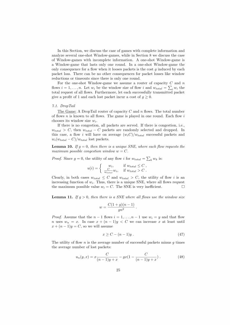
In this Section, we discuss the case of games with complete information andanalyze several one-shot Window-games, while in Section 8 we discuss the caseof Window-games with incomplete information. A one-shot Window-game isa Window-game that lasts only one round. In a one-shot Window-game theonly consequence for a flow when it looses packets is the cost g induced by eachpacket loss. There can be no other consequences for packet losses like windowreductions or timeouts since there is only one round.

For the one-shot Window-game we assume a router of capacity C and nflows i = 1, . . . , n. Let wi be the window size of flow i and wtotal =

∑i wi the

total request of all flows. Furthermore, let each successfully transmitted packetgive a profit of 1 and each lost packet incur a cost of g ≥ 0.

7.1. DropTailThe Game: A DropTail router of capacity C and n flows. The total number

of flows n is known to all flows. The game is played in one round. Each flow ichooses its window size wi.

If there is no congestion, all packets are served. If there is congestion, i.e.,wtotal > C, then wtotal − C packets are randomly selected and dropped. Inthis case, a flow i will have on average (wiC)/wtotal successful packets andwi(wtotal − C)/wtotal lost packets.

Lemma 10. If g = 0, then there is a unique SNE, where each flow requests themaximum possible congestion window w = C.

Proof. Since g = 0, the utility of any flow i for wtotal =∑

k wk is:

u(i) ={

wi, if wtotal ≤ C ,C

wtotalwi, if wtotal > C .

Clearly, in both cases wtotal ≤ C and wtotal > C, the utility of flow i is anincreasing function of wi. Thus, there is a unique SNE, where all flows requestthe maximum possible value wi = C. The SNE is very inefficient.

Lemma 11. If g > 0, then there is a SNE where all flows use the window size

w =C(1 + g)(n− 1)

gn2.

Proof. Assume that the n − 1 flows i = 1, . . . , n − 1 use wi = y and that flown uses wn = x. In case x + (n − 1)y < C we can increase x at least untilx + (n− 1)y = C, so we will assume

x ≥ C − (n− 1)y . (47)

The utility of flow n is the average number of successful packets minus g timesthe average number of lost packets:

un(y, x) = xC

(n− 1)y + x− gx(1− C

(n− 1)y + x) . (48)

25

The only positive root of the partial derivative of un(y, x) with respect to x is

x =gy(1− n) +

√Cgy(1 + g)(n− 1)g

. (49)

Setting x = y gives x = y = C(1+g)(n−1)gn2 . We conclude that there is a SNE at

w =C(1 + g)(n− 1)

gn2.

For example, if g = 1, C = 100 and n = 10, then the SNE is at w = 18.Experimental results are presented in Table 2.

A legitimate question is whether there are reasonable conditions, for whichthe fair share wi = C/n is a SNE. Using w ≤ C/n in Lemma 11 and solving forg gives g ≥ n− 1. This shows that the larger the number flows, the higher thecost g must be, in order to prevent an undesirable SNE. A sufficient condition onthe cost g that does not depend on the number of players n is g ≥ C−1 ≥ n−1.However, when g takes such large values the game degenerates. For example,if g ≥ C − 1, then almost any (not necessarily symmetric) profile with totalwindow size equal to C is a NE.

7.2. MaxMinThe Game: A MaxMin router of capacity C and n flows. The number n is

known to all flows. The game is played in one round. Each flow i chooses itswindow size wi.

Shenker showed in [31] that a MaxMin policy enforces a fair NE in a networkmodel where the flows are Poisson sources. In the Window-game model as well,the MaxMin policy leads the system to desirable equilibria. More precisely:

Lemma 12. In MaxMin, there is a SNE where all flows play wi = C/n. Ifg > 0, then this is the only NE of the game.

Proof. In MaxMin, a flow i does not loose any packet if wi does not exceedits fair share. Consequently, each flow i will request at least its fair share, i.e.,wi ≥ C/n. Thus, the total request wtotal will be at least wtotal ≥ C and no flowcan gain by playing a value larger than C/n. This implies that there is a SNEwhere each flow i plays the strategy wi = C/n. If there is a strictly positive costg > 0 for each packet loss, then the above SNE is the only NE of the game.

Clearly, the SNE where all flows request wi = C/n is the optimal solution forthe Window-game problem. As already discussed, the disadvantage of MaxMinis that it is a stateful policy that consumes too many computational resourcesto be applied in practice.

26

7.3. PrinceThe Game: A Prince router of capacity C and n flows. The total number

of flows n is known to all flows. The game is played in one round. Each flow ichooses its window size wi.

The behavior of Prince is very similar to MaxMin. Every flow i can safelyrequest its fair share C/n, so wi ≥ C/n. If a flow i requests wi > C/n, then itmay very well receive far less than its fair share (unlike MaxMin where it willreceive at least its fair share). Clearly, the profile where all flows play wi = C/nis a SNE. If the cost for packet loss is g > 0, then this is the only NE of thegame. Hence:

Lemma 13. If∑

i wi − C ≤ maxi wi then there is a SNE where all flows playwi = C/n. If g > 0, then this is the only NE of the game.

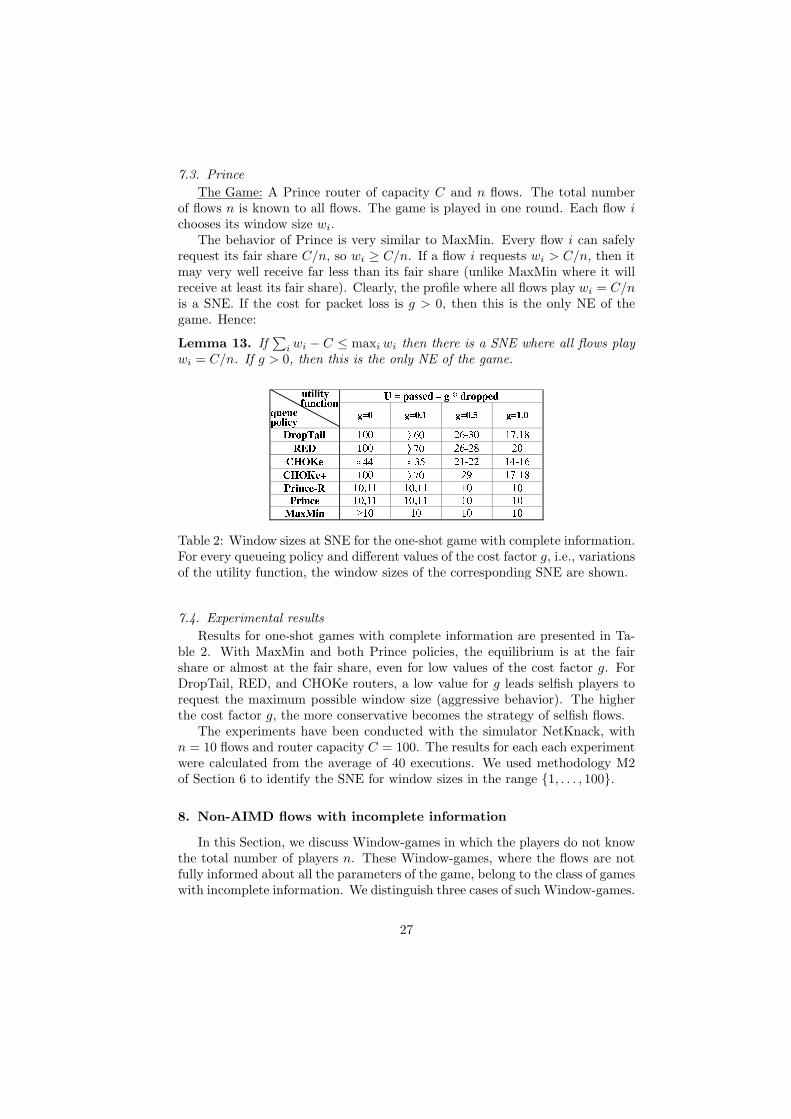
Table 2: Window sizes at SNE for the one-shot game with complete information.For every queueing policy and different values of the cost factor g, i.e., variationsof the utility function, the window sizes of the corresponding SNE are shown.

7.4. Experimental resultsResults for one-shot games with complete information are presented in Ta-

ble 2. With MaxMin and both Prince policies, the equilibrium is at the fairshare or almost at the fair share, even for low values of the cost factor g. ForDropTail, RED, and CHOKe routers, a low value for g leads selfish players torequest the maximum possible window size (aggressive behavior). The higherthe cost factor g, the more conservative becomes the strategy of selfish flows.

The experiments have been conducted with the simulator NetKnack, withn = 10 flows and router capacity C = 100. The results for each each experimentwere calculated from the average of 40 executions. We used methodology M2of Section 6 to identify the SNE for window sizes in the range {1, . . . , 100}.

8. Non-AIMD flows with incomplete information

In this Section, we discuss Window-games in which the players do not knowthe total number of players n. These Window-games, where the flows are notfully informed about all the parameters of the game, belong to the class of gameswith incomplete information. We distinguish three cases of such Window-games.

27

8.1. One-shot Window-game with no prior probabilitiesThe Game: A router of capacity C and n players. The players have no

prior probabilities on the number of players, that is, they have no distributioninformation for the unknown number n. The game is played in one round andeach player chooses its window size.

Note that in this case, where the players do not have distribution informationon the unknown parameters, the Nash equilibrium or the Bayes-Nash equilib-rium concepts cannot be applied. Several concepts, like games with no priorprobability or pre-Bayesian games [4, 1] have been proposed to capture gameswith no prior probabilities. One possibility is to search for an ex-post equilibrium,which is a profile where each player’s strategy is a best response to the otherplayer’s strategies, under all possible realizations of the uncertain data [1]. Inparticular, for the Window-games of this Section, each player’s strategy wouldbe a best response regardless of the number of participating players. Eventhough an ex-post equilibrium would be a very attractive solution, the problemis that, in general, ex post equilibria do not exist in incomplete-informationgames.

Other, more general, related equilibrium concepts are for example the safety-level equilibrium [4], the robust-optimization equilibrium [1], and the minimax-regret equilibrium. The common characteristic of these equilibrium concepts isthat the player selects a very conservative action. In this case, the players may,for example, assume that the number of players n is the maximum possiblenumber n = C. Hence, the players will play as in the game with completeinformation with n = C. For strategies like Prince and MaxMin, the choice ofeach player would be w = 1. Interestingly, in common TCP implementations,like Reno or Tahoe, flows start with a very conservative initial window sizew = 1.

8.2. One-shot Window-game with prior probabilitiesThe Game: A router of capacity C and n players. The number of players

n is a random variable and the players know the corresponding probabilitydistribution. The game is played in one round and each player i chooses itswindow size wi.

In practice, flows engaged in a TCP-game are likely to have some priorinformation on the number n or, equivalently, on their fair share. Note that realTCP flows are actually playing a repeated game, which means that the flowwill in most cases have an estimation on its fair share from the previous rounds(except of the first round or a round after some serious network change). If theflow has prior information on the distribution of the unknown parameter n, theresult is a Bayesian game. We leave the analysis of this and the following caseas future work.

8.3. Repeated Window-game with incomplete informationThe Game: A router of capacity C and n players. The number of players n

is unknown and probability distribution information on n may or may not begiven. Each player chooses its window size for each round of the game.

28

The motivation for this game comes from the fact that the actual gamethat a TCP flow has to play is a repeated game with incomplete information.The problem has been addressed from an optimization and an on-line algorithmpoint of view in [19]. One other approach would be to consider this as a learninggame; there are C players and nature decides for each player either to participatein the game or to stay idle. The goal of each participating player is to “learn”the unknown number n of players who participate.

We believe that a very interesting class of games that can also be used tomodel this case of Window-games, is the class of unknown games (for examplesee [6, Section 7.5]). In an unknown game, K players play a game repeatedly,and at each time instance t, after taking an action, player k observes his loss (orgain) but does not know his entire loss (or gain) function and cannot observethe other players’ actions. The player may not even know the number of playersparticipating in the game. Interestingly, even with such limited informationthere are conditions under which the game converges to a correlated equilibriumor even to a Nash equilibrium.

We may further define the dynamic version of this Window-game, where thenumber of participating players may change from round to round. In this case,in each round, nature decides with some predetermined probability for everyplayer to switch between the idle and the non-idle state.

9. Discussion

We present a game-theoretic model for the interplay between the congestionwindows of competing TCP flows. The theoretical analysis and the experimentalresults show that the model is relevant to the “real” TCP game. Furthermorewe propose a simple queue policy, called Prince, which can achieve efficient SNEdespite the presence of selfish flows.

Future work includes the completion of the analysis of Window-games withincomplete information. We also consider the proposed Prince policy of inde-pendent interest and intend to further study it. On the one hand, a thoroughanalysis of Prince presents an interesting problem, related to common resourceallocation games. On the other hand, we plan to investigate a realistic adapta-tion and implementation of Prince, possibly with streaming algorithms, on realTCP networks or with the network simulator [26].

Acknowledgements. We wish to thank Vasilis Tsaoussidis for insight-ful discussions on TCP congestion control and Lakis Papaschinopoulos for hisassistance in the proof of Lemma 6. We thank Evangelia Pyrga for bringingreference [6] to our attention.

References

[1] M. Aghassi and D. Bertsimas. Robust game theory. Math. Program.,107(1):231–273, 2006.

29

[2] A. Akella, S. Seshan, R. Karp, S. Shenker, and C. Papadimitriou. Selfishbehavior and stability of the internet: a game-theoretic analysis of tcp.In Proceedings of SIGCOMM 2002, pages 117–130, New York, NY, USA,2002. ACM Press.

[3] A. Akella, S. Seshan, S. Shenker, and I. Stoica. Exploring congestioncontrol. Technical Report CMU-CS-02-139, School of Computer Science,Carnegie Mellon University, Pittsburgh, Pennsylvania, May 2002.

[4] I. Ashlagi, D. Monderer, and M. Tennenholtz. Resource selection gameswith unknown number of players. In Proceedings of AAMAS ’06, pages819–825, New York, NY, USA, 2006. ACM Press.

[5] D. Bertsekas and R. Gallager. Data networks. Publication New Delhi,Prentice-Hall of India Pvt. Ltd., 1987.

[6] N. Cesa-Bianchi and G. Lugosi. Prediction, learning, and games. Cam-bridge University Press, 2006.

[7] D. Chiu and R. Jain. Analysis of the increase/decrease algorithms forcongestion avoidance in computer networks. j-COMP-NET-ISDN, 17(1):1–14, June 1989.

[8] P.S. Efraimidis and L. Tsavlidis. Window-games between tcp flows. InLecture Notes in Computer Science (SAGT 2008), volume 4997, pages 95–108, Springer-Verlag Berlin Heidelberg, 2008.

[9] K. Fall and S. Floyd. Simulation-based comparison of tahoe, reno, and sacktcp. Computer Communication Review, 26:5–21, 1996.

[10] S. Floyd and V. Jacobson. Random early detection gateways for congestionavoidance. IEEE/ACM Transactions on Networking, 1(4):397–413, August1993.

[11] D. Fotakis, S. Kontogiannis, E. Koutsoupias, M. Mavronicolas, and P. Spi-rakis. The structure and complexity of nash equilibria for a selfish routinggame. Theor. Comput. Sci., In Press, Corrected Proof:–, 2008.

[12] D. Fotakis, S. Kontogiannis, and P. Spirakis. Selfish unsplittable flows.Theor. Comput. Sci., 348(2):226–239, 2005.

[13] X. Gao, K. Jain, and L.J. Schulman. Fair and efficient router congestioncontrol. In SODA ’04: Proceedings of the fifteenth annual ACM-SIAM sym-posium on Discrete algorithms, pages 1050–1059, Philadelphia, PA, USA,2004. Society for Industrial and Applied Mathematics.

[14] R. Garg, A. Kamra, and V. Khurana. A game-theoretic approach towardscongestion control in communication networks. SIGCOMM Comput. Com-mun. Rev., 32(3):47–61, 2002.

30

[15] M. Habib, C. McDiarmid, J. Ramirez-Alfonsin, and B. Reed, editors. Prob-abilistic Methods for Algorithmic Discrete Mathematics. Springer, 1998.

[16] E.L. Hahne. Round-robin scheduling for max-min fairness in data networks.IEEE Journal of Selected Areas in Communications, 9(7):1024–1039, 1991.

[17] G. Hardin. The tragedy of the commons. Science, 162:1243–1248, 1968.

[18] V. Jacobson. Congestion avoidance and control. In Proceedings of SIG-COMM ’88, pages 314–329, New York, NY, USA, 1988. ACM.

[19] R. Karp, E. Koutsoupias, C. Papadimitriou, and S. Shenker. Optimizationproblems in congestion control. In Proceedings of FOCS ’00, page 66,Washington, DC, USA, 2000. IEEE Computer Society.

[20] R.J. La and V. Anantharam. Window-based congestion control with het-erogeneous users. In INFOCOM 2001, volume 3, pages 1320–1329. IEEE,2001.

[21] L. Lopez, G. del Rey Almansa, S. Paquelet, and A. Fernandez. A mathe-matical model for the tcp tragedy of the commons. Theor. Comput. Sci.,343(1-2):4–26, 2005.

[22] L. Lopez, A. Fernandez, and V. Cholvi. A game theoretic comparison oftcp and digital fountain based protocols. Comput. Netw., 51(12):3413–3426,2007.

[23] I. Milchtaich. Congestion games with player-specific payoff functions.Games and Economic Behavior, 13:111–124, 1996.

[24] D. Monderer and L. Shapley. Potential games. Games and EconomicBehavior, 14:124–143, 1996.

[25] NetKnack. A simulator for the window-game.http://utopia.duth.gr/∼pefraimi/projects/NetKnack.

[26] NS-2. The network simulator. http://www.isi.edu/nsnam/ns/.

[27] J. Padhye, V. Firoiu, D.F. Towsley, and J.F. Kurose. Modeling tcp renoperformance: a simple model and its empirical validation. IEEE/ACMTrans. Netw., 8(2):133–145, 2000.

[28] Rong Pan, Balaji Prabhakar, and Konstantinos Psounis. Choke, a state-less active queue management scheme for approximating fair bandwidthallocation. In INFOCOM, pages 942–951, 2000.

[29] C. Papadimitriou. Algorithms, games, and the internet. In STOC ’01:Proceedings of the thirty-third annual ACM symposium on Theory of com-puting, pages 749–753, New York, NY, USA, 2001. ACM Press.

31

[30] R.W. Rosenthal. A class of games possessing pure-strategy nash equilibria.International Journal of Game Theory, 2:65–67, 1973.

[31] S. J. Shenker. Making greed work in networks: a game-theoretic analysis ofswitch service disciplines. IEEE/ACM Trans. Netw., 3(6):819–831, 1995.

[32] I. Stoica, S. Shenker, and H. Zhang. Core-stateless fair queueing: achiev-ing approximately fair bandwidth allocations in high speed networks. SIG-COMM Comput. Commun. Rev., 28(4):118–130, 1998.

[33] I. Stoica and H. Zhang. Providing guaranteed services without per flowmanagement. SIGCOMM Comput. Commun. Rev., 29(4):81–94, 1999.

32

Window-Games between TCP °owsI - Utopia

Documents

Transcript of Window-Games between TCP °owsI - Utopia