
WIND CHARACTERISTICS - Solar Power | Solar Lighting | Solar
68
Chapter 2—Wind Characteristics 2–1 WIND CHARACTERISTICS The wind blows to the south and goes round to the north:, round and round goes the wind, and on its circuits the wind returns. Ecclesiastes 1:6 The earth’s atmosphere can be modeled as a gigantic heat engine. It extracts energy from one reservoir (the sun) and delivers heat to another reservoir at a lower temperature (space). In the process, work is done on the gases in the atmosphere and upon the earth-atmosphere boundary. There will be regions where the air pressure is temporarily higher or lower than average. This difference in air pressure causes atmospheric gases or wind to flow from the region of higher pressure to that of lower pressure. These regions are typically hundreds of kilometers in diameter. Solar radiation, evaporation of water, cloud cover, and surface roughness all play important roles in determining the conditions of the atmosphere. The study of the interactions between these effects is a complex subject called meteorology, which is covered by many excellent textbooks.[4, 8, 20] Therefore only a brief introduction to that part of meteorology concerning the flow of wind will be given in this text. 1 METEOROLOGY OF WIND The basic driving force of air movement is a difference in air pressure between two regions. This air pressure is described by several physical laws. One of these is Boyle’s law, which states that the product of pressure and volume of a gas at a constant temperature must be a constant, or p 1 V 1 = p 2 V 2 (1) Another law is Charles’ law, which states that, for constant pressure, the volume of a gas varies directly with absolute temperature. V 1 T 1 = V 2 T 2 (2) If a graph of volume versus temperature is made from measurements, it will be noticed that a zero volume state is predicted at −273.15 o C or 0 K. The laws of Charles and Boyle can be combined into the ideal gas law pV = nRT (3) Wind Energy Systems by Dr. Gary L. Johnson November 20, 2001
Transcript of WIND CHARACTERISTICS - Solar Power | Solar Lighting | Solar
Chapter 2—Wind Characteristics 2–1
WIND CHARACTERISTICS
The wind blows to the south and goes round to the north:, round and round goes the wind,and on its circuits the wind returns. Ecclesiastes 1:6
The earth’s atmosphere can be modeled as a gigantic heat engine. It extracts energy fromone reservoir (the sun) and delivers heat to another reservoir at a lower temperature (space).In the process, work is done on the gases in the atmosphere and upon the earth-atmosphereboundary. There will be regions where the air pressure is temporarily higher or lower thanaverage. This difference in air pressure causes atmospheric gases or wind to flow from theregion of higher pressure to that of lower pressure. These regions are typically hundreds ofkilometers in diameter.
Solar radiation, evaporation of water, cloud cover, and surface roughness all play importantroles in determining the conditions of the atmosphere. The study of the interactions betweenthese effects is a complex subject called meteorology, which is covered by many excellenttextbooks.[4, 8, 20] Therefore only a brief introduction to that part of meteorology concerningthe flow of wind will be given in this text.
1 METEOROLOGY OF WIND
The basic driving force of air movement is a difference in air pressure between two regions.This air pressure is described by several physical laws. One of these is Boyle’s law, whichstates that the product of pressure and volume of a gas at a constant temperature must be aconstant, or
p1V1 = p2V2 (1)
Another law is Charles’ law, which states that, for constant pressure, the volume of a gasvaries directly with absolute temperature.
V1
T1=
V2
T2(2)
If a graph of volume versus temperature is made from measurements, it will be noticedthat a zero volume state is predicted at −273.15oC or 0 K.
The laws of Charles and Boyle can be combined into the ideal gas law
pV = nRT (3)
Wind Energy Systems by Dr. Gary L. Johnson November 20, 2001
Chapter 2—Wind Characteristics 2–2
In this equation, R is the universal gas constant, T is the temperature in kelvins, V isthe volume of gas in m3, n is the number of kilomoles of gas, and p is the pressure in pascals(N/m2). At standard conditions, 0oC and one atmosphere, one kilomole of gas occupies 22.414m3 and the universal gas constant is 8314.5 J/(kmol·K) where J represents a joule or a newtonmeter of energy. The pressure of one atmosphere at 0oC is then
(8314.5J/(kmol · K))(273.15 K)22.414 m3
= 101, 325 Pa (4)
One kilomole is the amount of substance containing the same number of molecules as thereare atoms in 12 kg of the pure carbon nuclide 12C. In dry air, 78.09 % of the molecules arenitrogen, 20.95 % are oxygen, 0.93 % are argon, and the other 0.03 % are a mixture of CO2,Ne, Kr, Xe, He, and H2. This composition gives an average molecular mass of 28.97, so themass of one kilomole of dry air is 28.97 kg. For all ordinary purposes, dry air behaves like anideal gas.
The density ρ of a gas is the mass m of one kilomole divided by the volume V of thatkilomole.
ρ =m
V(5)
The volume of one kilomole varies with pressure and temperature as specified by Eq. 3.When we insert Eq. 3 into Eq. 5, the density is given by
ρ =mp
RT=
3.484pT
kg/m3 (6)
where p is in kPa and T is in kelvins. This expression yields a density for dry air at standardconditions of 1.293 kg/m3.
The common unit of pressure used in the past for meteorological work has been the bar(100 kPa) and the millibar (100 Pa). In this notation a standard atmosphere was referred toas 1.01325 bar or 1013.25 millibar.
Atmospheric pressure has also been given by the height of mercury in an evacuated tube.This height is 29.92 inches or 760 millimeters of mercury for a standard atmosphere. Thesenumbers may be useful in using instruments or reading literature of the pre-SI era. It may beworth noting here that several definitions of standard conditions are in use. The chemist uses0oC as standard temperature while engineers have often used 68oF (20oC) or 77oF (25oC) asstandard temperature. We shall not debate the respective merits of the various choices, butnote that some physical constants depend on the definition chosen, so that one must exercisecare in looking for numbers in published tables. In this text, standard conditions will alwaysbe 0oC and 101.3 kPa.
Within the atmosphere, there will be large regions of alternately high and low pressure.
Wind Energy Systems by Dr. Gary L. Johnson November 20, 2001
Chapter 2—Wind Characteristics 2–3
These regions are formed by complex mechanisms, which are still not fully understood. Solarradiation, surface cooling, humidity, and the rotation of the earth all play important roles.
In order for a high pressure region to be maintained while air is leaving it at ground level,there must be air entering the region at the same time. The only source for this air is abovethe high pressure region. That is, air will flow down inside a high pressure region (and upinside a low pressure region) to maintain the pressure. This descending air will be warmedadiabatically (i.e. without heat or mass transfer to its surroundings) and will tend to becomedry and clear. Inside the low pressure region, the rising air is cooled adiabatically, which mayresult in clouds and precipitation. This is why high pressure regions are usually associatedwith good weather and low pressure regions with bad weather.
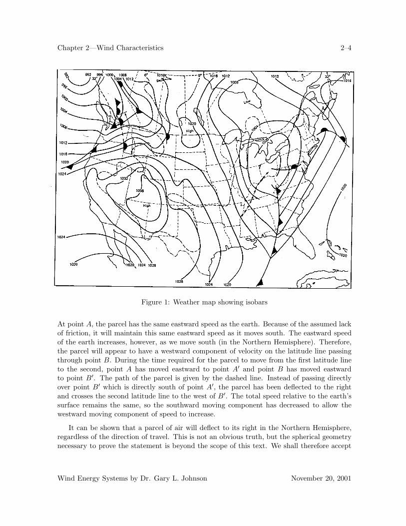
A line drawn through points of equal pressure on a weather map is called an isobar. Thesepressures are corrected to a common elevation such as sea level. For ease of plotting, theintervals between the isobars are usually 300, 400, or 500 Pa. Thus, successive isobars wouldbe drawn through points having readings of 100.0, 100.4, 100.8 kPa, etc. Such a map is shownin Fig. 1. This particular map of North America shows a low pressure region over the GreatLakes and a high pressure region over the Southwestern United States. There are two frontalsystems, one in the Eastern United States and one in the Pacific Northwest. The map showsa range of pressures between 992 millibars (99.2 kPa) and 1036 millibars (103.6 kPa). Thesepressures are all corrected to sea level to allow a common basis for comparison. This meansthere are substantial areas of the Western United States where the actual measured stationpressure is well below the value shown because of the station elevation above sea level.
The horizontal pressure difference provides the horizontal force or pressure gradient whichdetermines the speed and initial direction of wind motion. In describing the direction of thewind, we always refer to the direction of origin of the wind. That is, a north wind is blowingon us from the north and is going toward the south.
The greater the pressure gradient, the greater is the force on the air, and the higher is thewind speed. Since the direction of the force is from higher to lower pressure, and perpendicularto the isobars, the initial tendency of the wind is to blow parallel to the horizontal pressuregradient and perpendicular to the isobars. However, as soon as wind motion is established,a deflective force is produced which alters the direction of motion. This force is called theCoriolis force.
The Coriolis force is due to the earth’s rotation under a moving particle of air. From afixed observation point in space air would appear to travel in a straight line, but from ourvantage point on earth it appears to curve. To describe this change in observed direction, anequivalent force is postulated.
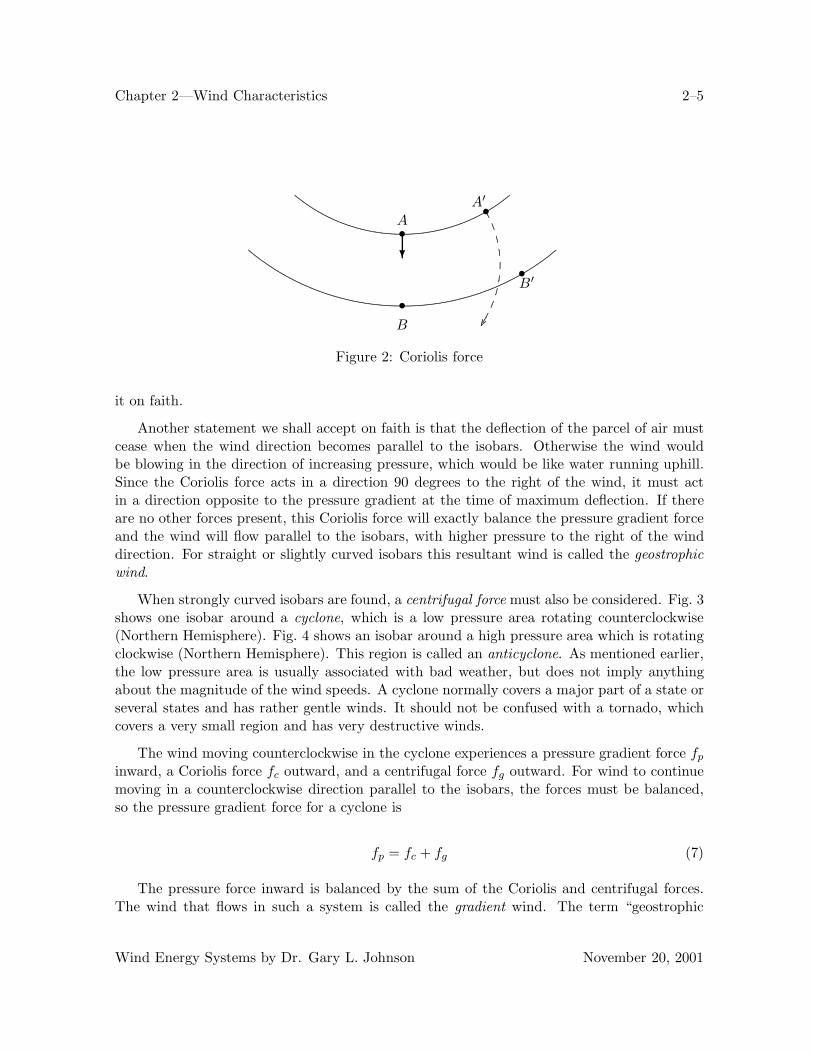
The basic effect is shown in Fig. 2. The two curved lines are lines of constant latitude, withpoint B located directly south of point A. A parcel of air (or some projectile like a cannonball) is moving south at point A. If we can imagine our parcel of air or our cannon ball to havezero air friction, then the speed of the parcel of air will remain constant with respect to theground. The direction will change, however, because of the earth’s rotation under the parcel.
Wind Energy Systems by Dr. Gary L. Johnson November 20, 2001
Chapter 2—Wind Characteristics 2–4
Figure 1: Weather map showing isobars
At point A, the parcel has the same eastward speed as the earth. Because of the assumed lackof friction, it will maintain this same eastward speed as it moves south. The eastward speedof the earth increases, however, as we move south (in the Northern Hemisphere). Therefore,the parcel will appear to have a westward component of velocity on the latitude line passingthrough point B. During the time required for the parcel to move from the first latitude lineto the second, point A has moved eastward to point A′ and point B has moved eastwardto point B′. The path of the parcel is given by the dashed line. Instead of passing directlyover point B′ which is directly south of point A′, the parcel has been deflected to the rightand crosses the second latitude line to the west of B′. The total speed relative to the earth’ssurface remains the same, so the southward moving component has decreased to allow thewestward moving component of speed to increase.
It can be shown that a parcel of air will deflect to its right in the Northern Hemisphere,regardless of the direction of travel. This is not an obvious truth, but the spherical geometrynecessary to prove the statement is beyond the scope of this text. We shall therefore accept
Wind Energy Systems by Dr. Gary L. Johnson November 20, 2001
Chapter 2—Wind Characteristics 2–5
...................................................................................................
...........................................
..................................
.............................................
.......................................................................................................................
..................................................
.......................................
.................................
...........................................................................
...................................................................................................
...........................................
..................................
............................
.................
.......................................................................................................................
..................................................
.......................................
.................................
.............................
...........................
...................
•
••
•
A
B
A′
B′
�
...........................................................................................
...........................................
..................
Figure 2: Coriolis force
it on faith.
Another statement we shall accept on faith is that the deflection of the parcel of air mustcease when the wind direction becomes parallel to the isobars. Otherwise the wind wouldbe blowing in the direction of increasing pressure, which would be like water running uphill.Since the Coriolis force acts in a direction 90 degrees to the right of the wind, it must actin a direction opposite to the pressure gradient at the time of maximum deflection. If thereare no other forces present, this Coriolis force will exactly balance the pressure gradient forceand the wind will flow parallel to the isobars, with higher pressure to the right of the winddirection. For straight or slightly curved isobars this resultant wind is called the geostrophicwind.
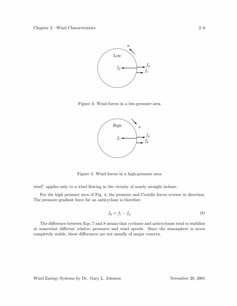
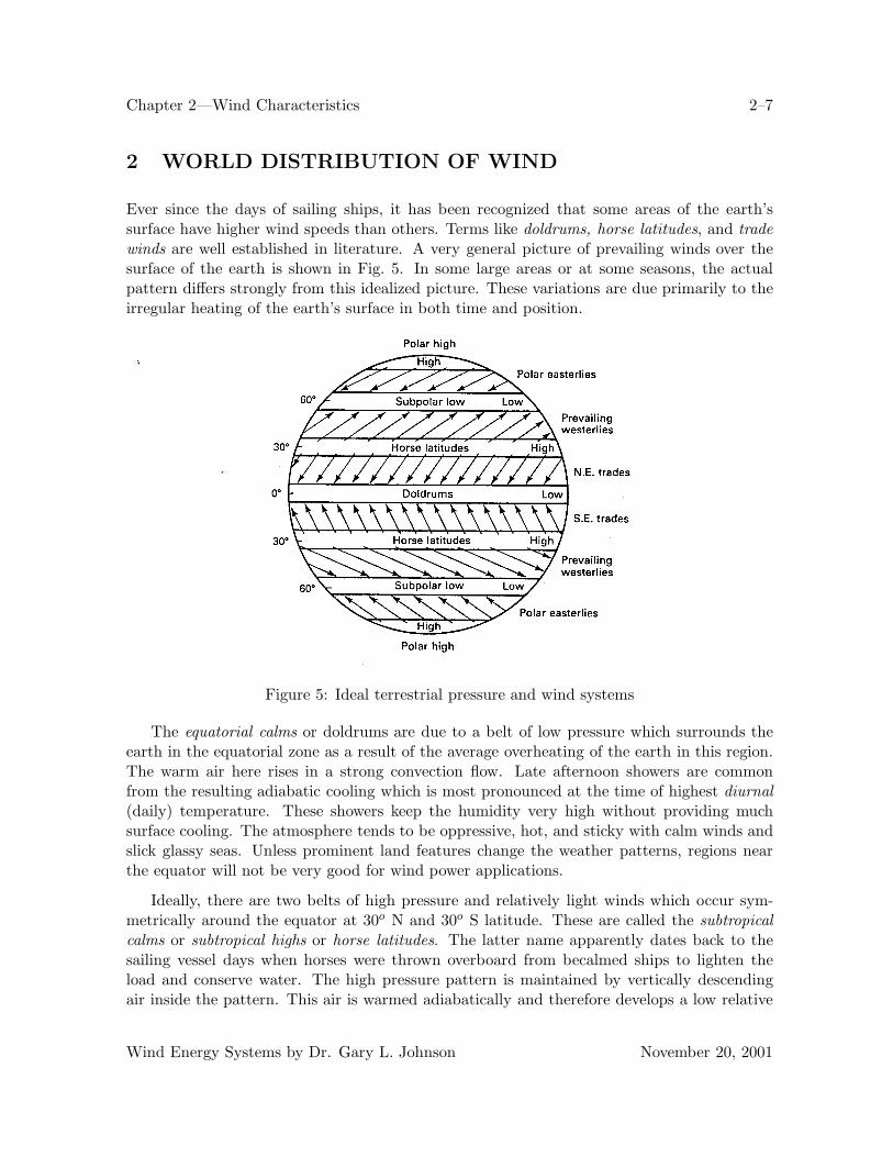
When strongly curved isobars are found, a centrifugal force must also be considered. Fig. 3shows one isobar around a cyclone, which is a low pressure area rotating counterclockwise(Northern Hemisphere). Fig. 4 shows an isobar around a high pressure area which is rotatingclockwise (Northern Hemisphere). This region is called an anticyclone. As mentioned earlier,the low pressure area is usually associated with bad weather, but does not imply anythingabout the magnitude of the wind speeds. A cyclone normally covers a major part of a state orseveral states and has rather gentle winds. It should not be confused with a tornado, whichcovers a very small region and has very destructive winds.
The wind moving counterclockwise in the cyclone experiences a pressure gradient force fp
inward, a Coriolis force fc outward, and a centrifugal force fg outward. For wind to continuemoving in a counterclockwise direction parallel to the isobars, the forces must be balanced,so the pressure gradient force for a cyclone is
fp = fc + fg (7)
The pressure force inward is balanced by the sum of the Coriolis and centrifugal forces.The wind that flows in such a system is called the gradient wind. The term “geostrophic
Wind Energy Systems by Dr. Gary L. Johnson November 20, 2001
Chapter 2—Wind Characteristics 2–6
........
........
........
................................................................
.......................
..............................
......................................................................................................................................................................................................................................................................................................................................................................................................................................................................................................................................
........................................................................................................................................
��
� fg
fcfp
Low���
u
Figure 3: Wind forces in a low-pressure area
........
........
........
..............................................................
.......................
............................
...........................................................................................................................................................................................................................................................................................................................................................................................................................................................................................................................................
.......................................................................................................................................
��
� fp
fgfc
High���
u
Figure 4: Wind forces in a high-pressure area
wind” applies only to a wind flowing in the vicinity of nearly straight isobars.
For the high pressure area of Fig. 4, the pressure and Coriolis forces reverse in direction.The pressure gradient force for an anticyclone is therefore
fp = fc − fg (8)
The difference between Eqs. 7 and 8 means that cyclones and anticyclones tend to stabilizeat somewhat different relative pressures and wind speeds. Since the atmosphere is nevercompletely stable, these differences are not usually of major concern.
Wind Energy Systems by Dr. Gary L. Johnson November 20, 2001
Chapter 2—Wind Characteristics 2–7
2 WORLD DISTRIBUTION OF WIND
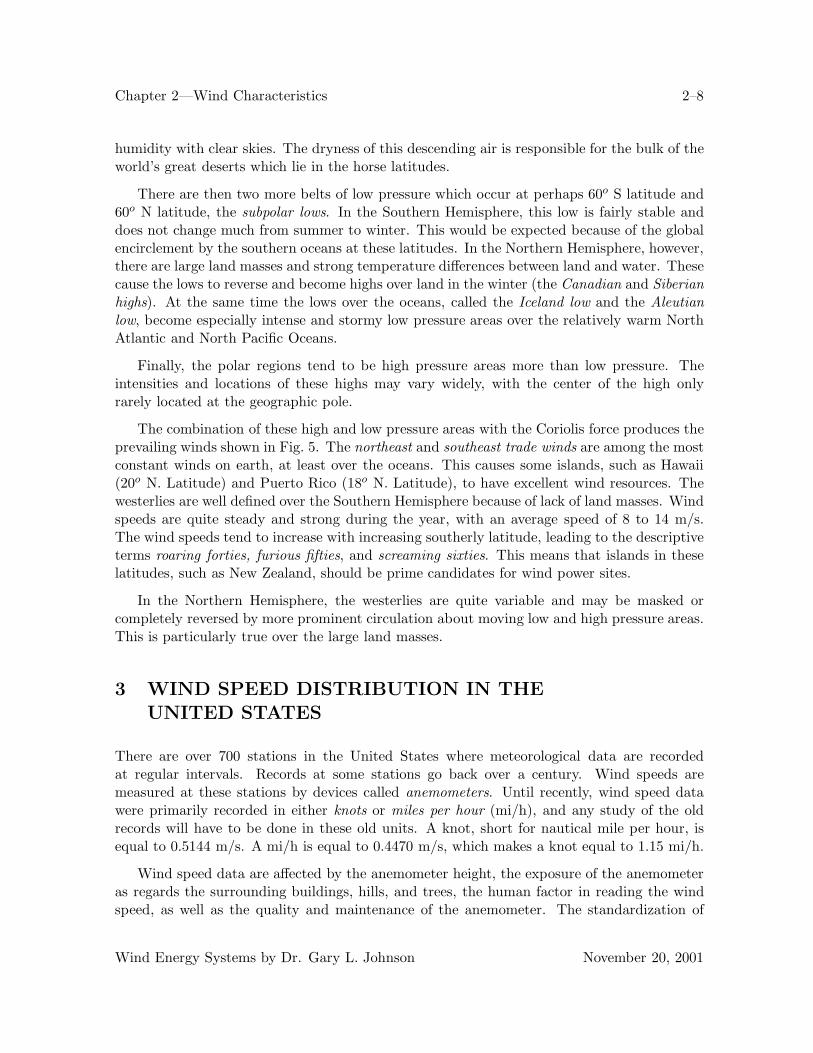
Ever since the days of sailing ships, it has been recognized that some areas of the earth’ssurface have higher wind speeds than others. Terms like doldrums, horse latitudes, and tradewinds are well established in literature. A very general picture of prevailing winds over thesurface of the earth is shown in Fig. 5. In some large areas or at some seasons, the actualpattern differs strongly from this idealized picture. These variations are due primarily to theirregular heating of the earth’s surface in both time and position.
Figure 5: Ideal terrestrial pressure and wind systems
The equatorial calms or doldrums are due to a belt of low pressure which surrounds theearth in the equatorial zone as a result of the average overheating of the earth in this region.The warm air here rises in a strong convection flow. Late afternoon showers are commonfrom the resulting adiabatic cooling which is most pronounced at the time of highest diurnal(daily) temperature. These showers keep the humidity very high without providing muchsurface cooling. The atmosphere tends to be oppressive, hot, and sticky with calm winds andslick glassy seas. Unless prominent land features change the weather patterns, regions nearthe equator will not be very good for wind power applications.
Ideally, there are two belts of high pressure and relatively light winds which occur sym-metrically around the equator at 30o N and 30o S latitude. These are called the subtropicalcalms or subtropical highs or horse latitudes. The latter name apparently dates back to thesailing vessel days when horses were thrown overboard from becalmed ships to lighten theload and conserve water. The high pressure pattern is maintained by vertically descendingair inside the pattern. This air is warmed adiabatically and therefore develops a low relative
Wind Energy Systems by Dr. Gary L. Johnson November 20, 2001
Chapter 2—Wind Characteristics 2–8
humidity with clear skies. The dryness of this descending air is responsible for the bulk of theworld’s great deserts which lie in the horse latitudes.
There are then two more belts of low pressure which occur at perhaps 60o S latitude and60o N latitude, the subpolar lows. In the Southern Hemisphere, this low is fairly stable anddoes not change much from summer to winter. This would be expected because of the globalencirclement by the southern oceans at these latitudes. In the Northern Hemisphere, however,there are large land masses and strong temperature differences between land and water. Thesecause the lows to reverse and become highs over land in the winter (the Canadian and Siberianhighs). At the same time the lows over the oceans, called the Iceland low and the Aleutianlow, become especially intense and stormy low pressure areas over the relatively warm NorthAtlantic and North Pacific Oceans.
Finally, the polar regions tend to be high pressure areas more than low pressure. Theintensities and locations of these highs may vary widely, with the center of the high onlyrarely located at the geographic pole.
The combination of these high and low pressure areas with the Coriolis force produces theprevailing winds shown in Fig. 5. The northeast and southeast trade winds are among the mostconstant winds on earth, at least over the oceans. This causes some islands, such as Hawaii(20o N. Latitude) and Puerto Rico (18o N. Latitude), to have excellent wind resources. Thewesterlies are well defined over the Southern Hemisphere because of lack of land masses. Windspeeds are quite steady and strong during the year, with an average speed of 8 to 14 m/s.The wind speeds tend to increase with increasing southerly latitude, leading to the descriptiveterms roaring forties, furious fifties, and screaming sixties. This means that islands in theselatitudes, such as New Zealand, should be prime candidates for wind power sites.
In the Northern Hemisphere, the westerlies are quite variable and may be masked orcompletely reversed by more prominent circulation about moving low and high pressure areas.This is particularly true over the large land masses.
3 WIND SPEED DISTRIBUTION IN THEUNITED STATES
There are over 700 stations in the United States where meteorological data are recordedat regular intervals. Records at some stations go back over a century. Wind speeds aremeasured at these stations by devices called anemometers. Until recently, wind speed datawere primarily recorded in either knots or miles per hour (mi/h), and any study of the oldrecords will have to be done in these old units. A knot, short for nautical mile per hour, isequal to 0.5144 m/s. A mi/h is equal to 0.4470 m/s, which makes a knot equal to 1.15 mi/h.
Wind speed data are affected by the anemometer height, the exposure of the anemometeras regards the surrounding buildings, hills, and trees, the human factor in reading the windspeed, as well as the quality and maintenance of the anemometer. The standardization of
Wind Energy Systems by Dr. Gary L. Johnson November 20, 2001
Chapter 2—Wind Characteristics 2–9
these factors has not been well enforced over the years. For example, the standard anemometerheight is 10 m but other heights are often found. In one study [16], six Kansas stations withdata available from 1948 to 1976 had 21 different anemometer heights, none of which was 10m. The only station which did not change anemometer height during this period was Russell,at a 9 m height. Heights ranged from 6 m to 22 m. The anemometer height at Topeka changedfive times, with heights of 17.7, 22.3, 17.7, 22.0, and 7.6 m.
Reported wind data therefore need to be viewed with some caution. Only when anemome-ter heights and surrounding obstructions are the same can two sites be fairly compared forwind power potential. Reported data can be used, of course, to give an indication of the bestregions of the country, with local site surveys being desirable to determine the quality of apotential wind power site.
Table 2.1 shows wind data for several stations in the United States. Similar data areavailable for most other U. S. stations. The percentage of time that the wind speed wasrecorded in a given speed range is given, as well as the mean speed and the peak speed[3].Each range of wind speed is referred to as a speed group. Wind speeds were always recordedin integer knots or integer mi/h, hence the integer nature of the speed groups. If wind speedswere recorded in knots instead of the mi/h shown, the size of the speed groups would beadjusted so the percentage in each group remains the same. The speed groups for windspeeds in knots are 1-3, 4-6, 7-10, 11-16, 17-21, 22-27, 28-33, 34-40, and 41-47 knots. Whenconverting wind data to mi/h speed groups, a 6 knot (6.91 mi/h) wind is assigned to thespeed group containing 7 mi/h, while a 7 knot (8.06 mi/h) wind is assigned to the 8-12 mi/hspeed group. Having the same percentages for two different unit systems is a help for somecomputations.
This table was prepared for the ten year period of 1951-60. No such tabulation wasprepared by the U. S. Environmental Data and Information Service for 1961-70 or 1971-80,and no further tabulation is planned until it appears that the long term climate has changedenough to warrant the expense of such a compilation.
It may be seen that the mean wind speed varies by over a factor of two, from 3.0 m/s inLos Angeles to 7.8 m/s in Cold Bay, Alaska. The power in the wind is proportional to thecube of the wind speed, as we shall see in Chapter 4, so a wind of 7.8 m/s has 17.6 times theavailable power as a 3.0 m/s wind. This does not mean that Cold Bay is exactly 17.6 timesas good as Los Angeles as a wind power site because of other factors to be considered later,but it does indicate a substantial difference.
The peak speed shown in Table 2.1 is the average speed of the fastest mile of air (1.6 km)to pass through a run of wind anemometer and is not the instantaneous peak speed of thepeak gust, which will be higher. This type of anemometer will be discussed in Chapter 3.
The Environmental Data and Information Service also has wind speed data available onmagnetic tape for many recording stations. This magnetic tape contains the complete recordof a station over a period of up to ten years, including such items as temperature, air pressure,and humidity in addition to wind speed and direction. These data are typically recorded once
Wind Energy Systems by Dr. Gary L. Johnson November 20, 2001

Chapter 2—Wind Characteristics 2–10
TABLE 2.1 Annual Percentage Frequency of Wind by Speed Groups and the Mean Speeda
Mean Peak0–3 4–7 8–12 13–18 19–24 25–31 32–38 Speed Speedb
Station mi/h mi/h mi/h mi/h mi/h mi/h mi/h (mi/h) (m/s)Albuquerque 17 36 26 13 5 2 8.6 40.2Amarillo 5 15 32 32 12 4 1 12.9 37.5Boise 15 30 32 18 4 1 8.9 27.3Boston 3 12 33 35 12 4 1 13.3 38.9Buffalo 5 17 34 27 13 3 1 12.4 40.7Casper 8 16 27 27 13 7 2 13.3 NAChicago(O’Hare) 8 22 33 27 8 2 11.2 38.9Cleveland 7 18 35 29 9 2 11.6 34.9Cold Bay 4 9 18 27 21 14 5 17.4 NADenver 11 27 34 22 5 2 10.0 29.0Des Moines 3 17 38 29 10 3 1 12.1 34.0Fargo 4 13 28 31 15 7 2 14.4 51.4Ft. Worth 4 14 34 34 10 3 12.5 30.4Great Falls 7 19 24 24 15 9 3 13.9 36.6Honolulu 9 17 27 32 12 2 12.1 30.0Kansas City 9 29 35 23 5 1 9.8 32.2Los Angeles 28 33 27 11 1 6.8 21.9Miami 14 20 34 20 2 8.8 59.0Minneapolis 8 21 34 28 9 2 11.2 41.1Oklahoma City 2 11 34 34 13 6 1 14.0 38.9Topeka 11 19 30 27 10 2 11.2 36.2Wake Island 1 6 27 48 17 2 14.6 NAWichita 4 12 30 31 16 5 1 13.7 44.7
aSource: Climatography of the United States, Series 82: Decennial Census of the United State Climate,“Summary of Hourly Observations, 1951–1960” (Table B).
bNA, not available
an hour but the magnetic tape only has data for every third hour, so there are eight windspeeds and eight wind directions per day available on the magnetic tape.
The available data can be summarized in other forms besides that of Table 2.1. One formis the speed-duration curve as shown in Fig. 6. The horizontal axis is in hours per year, witha maximum value of 8760 for a year with 365 days. The vertical axis gives the wind speedthat is exceeded for the number of hours per year on the horizontal axis. For Dodge City,Kansas, for example, a wind speed of 4 m/s is exceeded 6500 hours per year while 10 m/s isexceeded 700 hours per year. For Kansas City, 4 m/s is exceeded 4460 hours and 10 m/s isexceeded only 35 hours a year. Dodge City is seen to be a better location for a wind turbine
Wind Energy Systems by Dr. Gary L. Johnson November 20, 2001
Chapter 2—Wind Characteristics 2–11
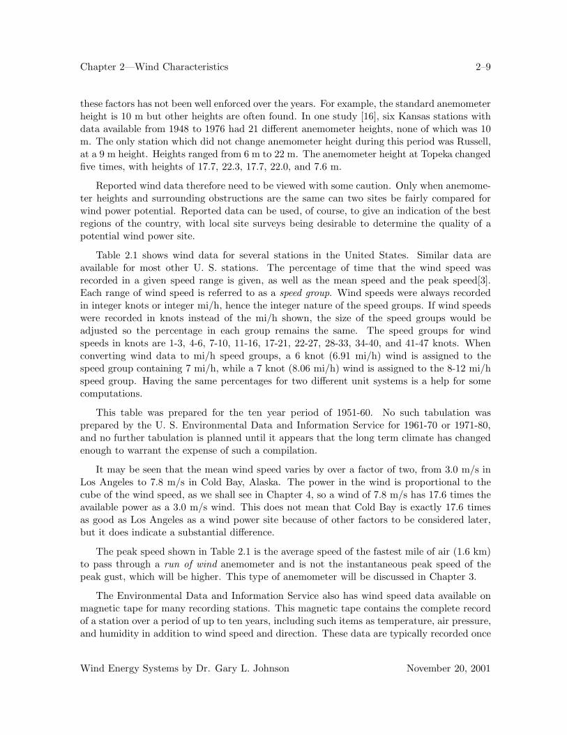
than Kansas City. Dodge City had a mean wind speed for this year of 5.68 m/s while KansasCity had a mean wind speed of 3.82 m/s. The anemometer height for both stations was 7 mabove the ground.
Figure 6: Speed-duration curves, 1970
Speed duration curves can be used to determine the number of hours of operation of aspecific wind turbine. A wind turbine that starts producing power at 4 m/s and reaches ratedpower at 10 m/s would be operating 6500 hours per year at Dodge City (for the data shownin Fig. 6 and would be producing rated output for 700 of these hours. The output would beless than rated for the intermediate 5800 hours.
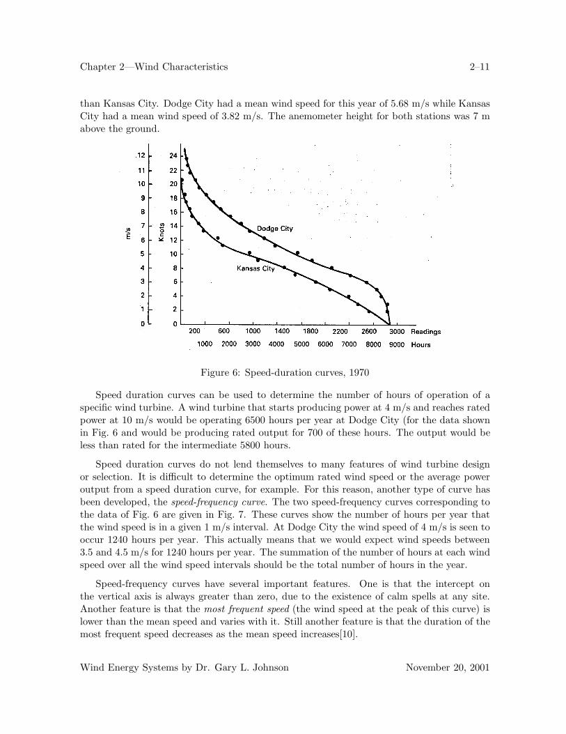
Speed duration curves do not lend themselves to many features of wind turbine designor selection. It is difficult to determine the optimum rated wind speed or the average poweroutput from a speed duration curve, for example. For this reason, another type of curve hasbeen developed, the speed-frequency curve. The two speed-frequency curves corresponding tothe data of Fig. 6 are given in Fig. 7. These curves show the number of hours per year thatthe wind speed is in a given 1 m/s interval. At Dodge City the wind speed of 4 m/s is seen tooccur 1240 hours per year. This actually means that we would expect wind speeds between3.5 and 4.5 m/s for 1240 hours per year. The summation of the number of hours at each windspeed over all the wind speed intervals should be the total number of hours in the year.
Speed-frequency curves have several important features. One is that the intercept onthe vertical axis is always greater than zero, due to the existence of calm spells at any site.Another feature is that the most frequent speed (the wind speed at the peak of this curve) islower than the mean speed and varies with it. Still another feature is that the duration of themost frequent speed decreases as the mean speed increases[10].
Wind Energy Systems by Dr. Gary L. Johnson November 20, 2001
Chapter 2—Wind Characteristics 2–12
Figure 7: Speed-frequency curves, 1970
Speed frequency curves, or similar mathematical functions, can be used in studies todevelop estimates of the seasonal and annual available wind power density in the UnitedStates and elsewhere. This is the power density in the wind in W/m2 of area perpendicularto the flow of air. It is always substantially more than the power density that can actuallybe extracted from the wind, as we shall see in Chapter 4. The result of one such study[9] isshown in Fig. 8. This shows the estimated annual average power density available in the windin W/m2 at an elevation of 50 m above ground. Few wind data are recorded at that height, sothe wind speeds at the actual anemometer heights have been extrapolated to 50 m by usingthe one-seventh power law, which will be discussed later in this chapter.
The shaded areas indicate mountainous terrain in which the wind power density estimatesrepresent lower limits for exposed ridges and mountain tops. (From [9])
The map shows that the good wind regions are the High Plains (a north-south strip about500 km wide on the east side of the Rocky Mountains), and mountain tops and exposed ridgesthroughout the country. The coastal regions in both the northeastern and northwestern UnitedStates are also good. There is a definite trend toward higher wind power densities at higherlatitudes, as would be expected from Fig. 5. The southeastern United States is seen to bequite low compared with the remainder of the country.
There are selected sites, of course, which cannot be shown on this map scale, but which
Wind Energy Systems by Dr. Gary L. Johnson November 20, 2001

Chapter 2—Wind Characteristics 2–13
Figure 8: Annual mean wind power density W/m2 estimated at 50 m above exposed areas.
have much higher wind power densities. Mt. Washington in New Hampshire has an averagewind speed of over 15 m/s, twice that of the best site in Table 2.1. The annual average windpower density there would be over 3000 W/m2. Mt. Washington also has the distinction ofhaving experienced the highest wind speed recorded at a regular weather data station, 105m/s (234 mi/h). Extreme winds plus severe icing conditions make this particular site a realchallenge for the wind turbine designer. Other less severe sites are being developed first forthese reasons.
Superior sites include mountain passes as well as mountain peaks. When a high or lowpressure air mass arrives at a mountain barrier, the air is forced to flow either over the moun-tain tops or through the passes. A substantial portion flows through the passes, with resultinghigh speed winds. The mountain passes are also usually more accessible than mountain peaksfor construction and maintenance of wind turbines. One should examine each potential sitecarefully in order to assure that it has good wind characteristics before installing any windturbines. Several sites should be investigated if possible and both hills and valleys should beconsidered.
Wind Energy Systems by Dr. Gary L. Johnson November 20, 2001
Chapter 2—Wind Characteristics 2–14
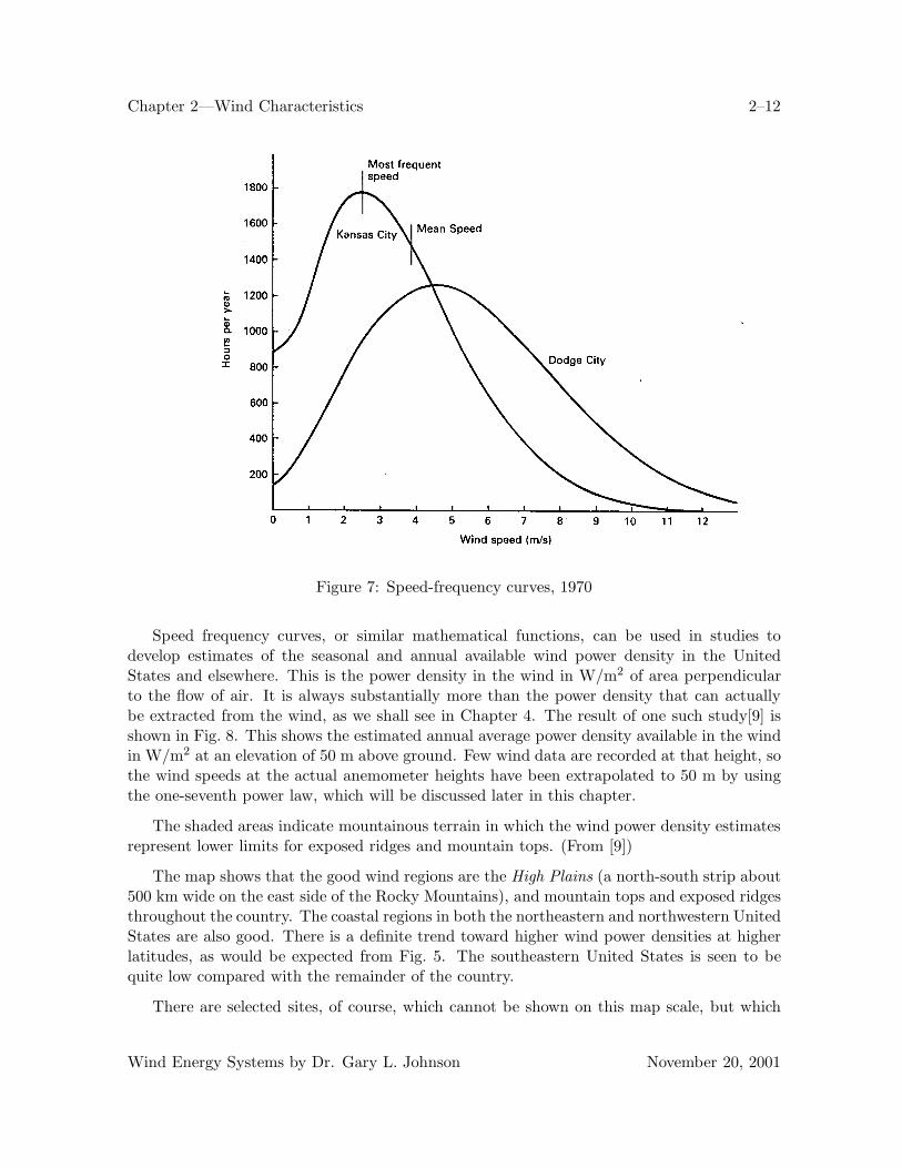
4 ATMOSPHERIC STABILITY
As we have mentioned, most wind speed measurements are made about 10 m above the ground.Small wind turbines are typically mounted 20 to 30 m above ground level, while the propellertip may reach a height of more than 100 m on the large turbines, so an estimate of wind speedvariation with height is needed. The mathematical form of this variation will be consideredin the next section, but first we need to examine a property of the atmosphere which controlsthis vertical variation of wind speed. This property is called atmospheric stability, which refersto the amount of mixing present in the atmosphere. We start this discussion by examiningthe pressure variation with height in the lower atmosphere
A given parcel of air has mass and is attracted to the earth by the force of gravity. For theparcel not to fall to the earth’s surface, there must be an equal and opposite force directedaway from the earth. This force comes from the decrease in air pressure with increasing height.The greater the density of air, the more rapidly must pressure decrease upward to hold theair at constant height against the force of gravity. Therefore, pressure decreases quickly withheight at low altitudes, where density is high, and slowly at high altitudes where density islow. This balanced force condition is called hydrostatic balance or hydrostatic equilibrium.
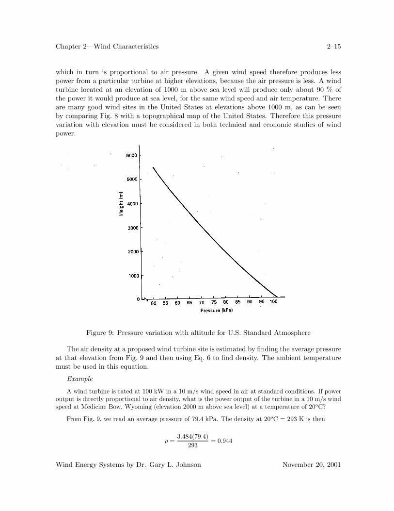
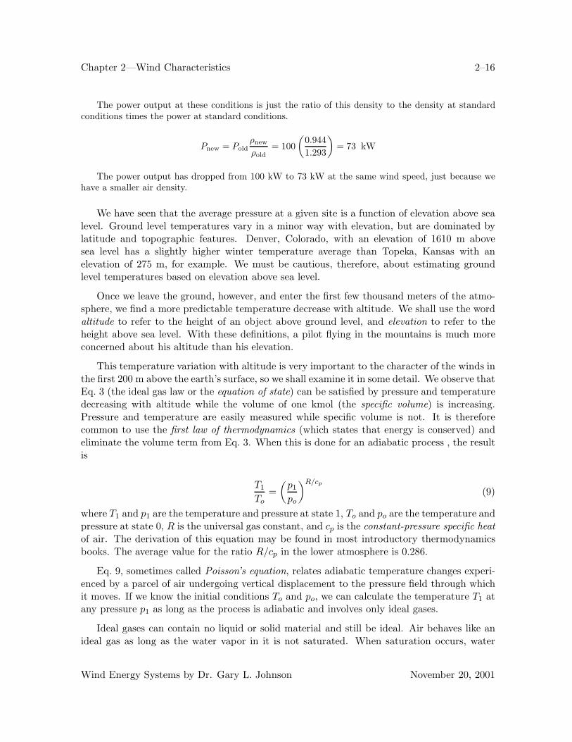
The average atmospheric pressure as a function of elevation above sea level for middlelatitudes is shown in Fig. 9. This curve is part of the model for the U.S. Standard Atmosphere.At sea level and a temperature of 273 K, the average pressure is 101.3 kPa, as mentionedearlier. A pressure of half this value is reached at about 5500 m. This pressure change withelevation is especially noticeable when flying in an airplane, when one’s ears tend to ‘pop’ asthe airplane changes altitude.
It should be noticed that the independent variable z is plotted on the vertical axis in thisfigure, while the dependent variable is plotted along the horizontal axis. It is plotted this waybecause elevation is intuitively up. To read the graph when the average pressure at a givenheight is desired, just enter the graph at the specified height, proceed horizontally until youhit the curve, and then go vertically downward to read the value of pressure.
The pressure in Fig. 9 is assumed to not vary with local temperature. That is, it is assumedthat the column of air directly above the point of interest maintains the same mass throughoutany temperature cycle. A given mass of air above some point will produce a constant pressureregardless of the temperature. The volume of gas in the column will change with temperaturebut not the pressure exerted by the column. This is not a perfect assumption because, whilethe mass of the entire atmosphere does not vary with temperature, the mass directly overheadwill vary somewhat with temperature. A temperature decrease of 30oC will often be associatedwith a pressure increase of 2 to 3 kPa. The atmospheric pressure tends to be a little higherin the early morning than in the middle of the afternoon. Winter pressures tend to be higherthan summer pressures. This effect is smaller than the pressure variation due to movementof weather patterns, hence will be ignored in this text.
It will be seen later that the power output of a wind turbine is proportional to air density,
Wind Energy Systems by Dr. Gary L. Johnson November 20, 2001
Chapter 2—Wind Characteristics 2–15
which in turn is proportional to air pressure. A given wind speed therefore produces lesspower from a particular turbine at higher elevations, because the air pressure is less. A windturbine located at an elevation of 1000 m above sea level will produce only about 90 % ofthe power it would produce at sea level, for the same wind speed and air temperature. Thereare many good wind sites in the United States at elevations above 1000 m, as can be seenby comparing Fig. 8 with a topographical map of the United States. Therefore this pressurevariation with elevation must be considered in both technical and economic studies of windpower.
Figure 9: Pressure variation with altitude for U.S. Standard Atmosphere
The air density at a proposed wind turbine site is estimated by finding the average pressureat that elevation from Fig. 9 and then using Eq. 6 to find density. The ambient temperaturemust be used in this equation.
Example
A wind turbine is rated at 100 kW in a 10 m/s wind speed in air at standard conditions. If poweroutput is directly proportional to air density, what is the power output of the turbine in a 10 m/s windspeed at Medicine Bow, Wyoming (elevation 2000 m above sea level) at a temperature of 20oC?
From Fig. 9, we read an average pressure of 79.4 kPa. The density at 20oC = 293 K is then
ρ =3.484(79.4)
293= 0.944
Wind Energy Systems by Dr. Gary L. Johnson November 20, 2001
Chapter 2—Wind Characteristics 2–16
The power output at these conditions is just the ratio of this density to the density at standardconditions times the power at standard conditions.
Pnew = Poldρnew
ρold= 100
(0.9441.293
)= 73 kW
The power output has dropped from 100 kW to 73 kW at the same wind speed, just because wehave a smaller air density.
We have seen that the average pressure at a given site is a function of elevation above sealevel. Ground level temperatures vary in a minor way with elevation, but are dominated bylatitude and topographic features. Denver, Colorado, with an elevation of 1610 m abovesea level has a slightly higher winter temperature average than Topeka, Kansas with anelevation of 275 m, for example. We must be cautious, therefore, about estimating groundlevel temperatures based on elevation above sea level.
Once we leave the ground, however, and enter the first few thousand meters of the atmo-sphere, we find a more predictable temperature decrease with altitude. We shall use the wordaltitude to refer to the height of an object above ground level, and elevation to refer to theheight above sea level. With these definitions, a pilot flying in the mountains is much moreconcerned about his altitude than his elevation.
This temperature variation with altitude is very important to the character of the winds inthe first 200 m above the earth’s surface, so we shall examine it in some detail. We observe thatEq. 3 (the ideal gas law or the equation of state) can be satisfied by pressure and temperaturedecreasing with altitude while the volume of one kmol (the specific volume) is increasing.Pressure and temperature are easily measured while specific volume is not. It is thereforecommon to use the first law of thermodynamics (which states that energy is conserved) andeliminate the volume term from Eq. 3. When this is done for an adiabatic process , the resultis
T1
To=(
p1
po
)R/cp
(9)
where T1 and p1 are the temperature and pressure at state 1, To and po are the temperature andpressure at state 0, R is the universal gas constant, and cp is the constant-pressure specific heatof air. The derivation of this equation may be found in most introductory thermodynamicsbooks. The average value for the ratio R/cp in the lower atmosphere is 0.286.
Eq. 9, sometimes called Poisson’s equation, relates adiabatic temperature changes experi-enced by a parcel of air undergoing vertical displacement to the pressure field through whichit moves. If we know the initial conditions To and po, we can calculate the temperature T1 atany pressure p1 as long as the process is adiabatic and involves only ideal gases.
Ideal gases can contain no liquid or solid material and still be ideal. Air behaves like anideal gas as long as the water vapor in it is not saturated. When saturation occurs, water
Wind Energy Systems by Dr. Gary L. Johnson November 20, 2001
Chapter 2—Wind Characteristics 2–17
starts to condense, and in condensing gives up its latent heat of vaporization. This heat energyinput violates the adiabatic constraint, while the presence of liquid water keeps air from beingan ideal gas.
Example
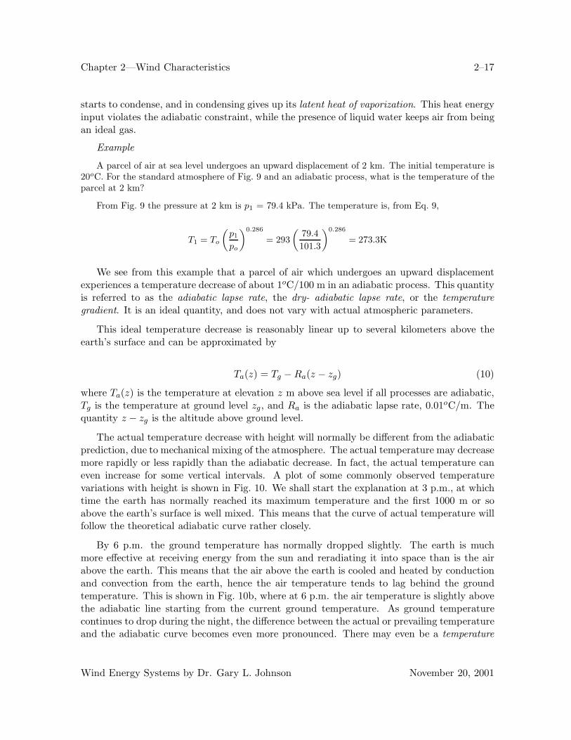
A parcel of air at sea level undergoes an upward displacement of 2 km. The initial temperature is20oC. For the standard atmosphere of Fig. 9 and an adiabatic process, what is the temperature of theparcel at 2 km?
From Fig. 9 the pressure at 2 km is p1 = 79.4 kPa. The temperature is, from Eq. 9,
T1 = To
(p1
po
)0.286
= 293(
79.4101.3
)0.286
= 273.3K
We see from this example that a parcel of air which undergoes an upward displacementexperiences a temperature decrease of about 1oC/100 m in an adiabatic process. This quantityis referred to as the adiabatic lapse rate, the dry- adiabatic lapse rate, or the temperaturegradient. It is an ideal quantity, and does not vary with actual atmospheric parameters.
This ideal temperature decrease is reasonably linear up to several kilometers above theearth’s surface and can be approximated by
Ta(z) = Tg − Ra(z − zg) (10)
where Ta(z) is the temperature at elevation z m above sea level if all processes are adiabatic,Tg is the temperature at ground level zg, and Ra is the adiabatic lapse rate, 0.01oC/m. Thequantity z − zg is the altitude above ground level.
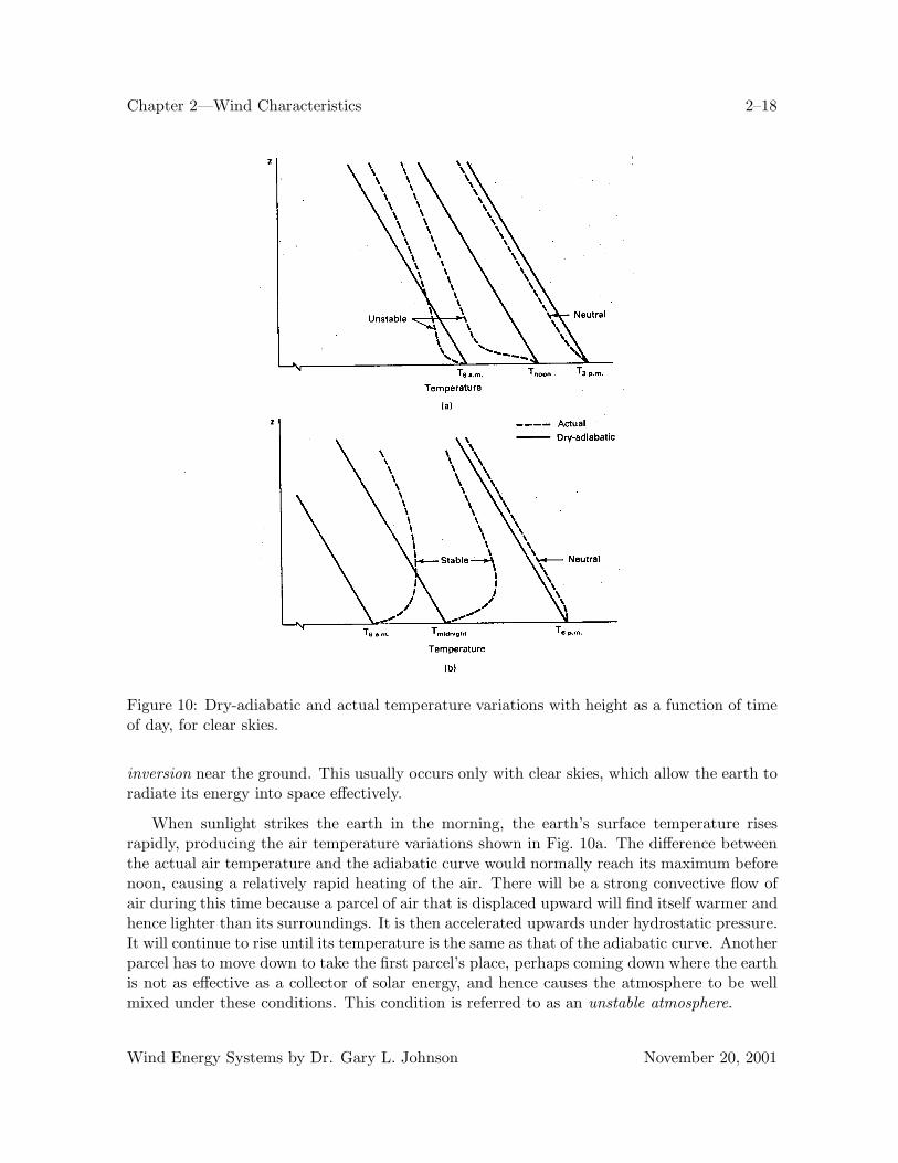
The actual temperature decrease with height will normally be different from the adiabaticprediction, due to mechanical mixing of the atmosphere. The actual temperature may decreasemore rapidly or less rapidly than the adiabatic decrease. In fact, the actual temperature caneven increase for some vertical intervals. A plot of some commonly observed temperaturevariations with height is shown in Fig. 10. We shall start the explanation at 3 p.m., at whichtime the earth has normally reached its maximum temperature and the first 1000 m or soabove the earth’s surface is well mixed. This means that the curve of actual temperature willfollow the theoretical adiabatic curve rather closely.
By 6 p.m. the ground temperature has normally dropped slightly. The earth is muchmore effective at receiving energy from the sun and reradiating it into space than is the airabove the earth. This means that the air above the earth is cooled and heated by conductionand convection from the earth, hence the air temperature tends to lag behind the groundtemperature. This is shown in Fig. 10b, where at 6 p.m. the air temperature is slightly abovethe adiabatic line starting from the current ground temperature. As ground temperaturecontinues to drop during the night, the difference between the actual or prevailing temperatureand the adiabatic curve becomes even more pronounced. There may even be a temperature
Wind Energy Systems by Dr. Gary L. Johnson November 20, 2001
Chapter 2—Wind Characteristics 2–18
Figure 10: Dry-adiabatic and actual temperature variations with height as a function of timeof day, for clear skies.
inversion near the ground. This usually occurs only with clear skies, which allow the earth toradiate its energy into space effectively.
When sunlight strikes the earth in the morning, the earth’s surface temperature risesrapidly, producing the air temperature variations shown in Fig. 10a. The difference betweenthe actual air temperature and the adiabatic curve would normally reach its maximum beforenoon, causing a relatively rapid heating of the air. There will be a strong convective flow ofair during this time because a parcel of air that is displaced upward will find itself warmer andhence lighter than its surroundings. It is then accelerated upwards under hydrostatic pressure.It will continue to rise until its temperature is the same as that of the adiabatic curve. Anotherparcel has to move down to take the first parcel’s place, perhaps coming down where the earthis not as effective as a collector of solar energy, and hence causes the atmosphere to be wellmixed under these conditions. This condition is referred to as an unstable atmosphere.
Wind Energy Systems by Dr. Gary L. Johnson November 20, 2001
Chapter 2—Wind Characteristics 2–19
On clear nights, however, the earth will be colder than the air above it, so a parcel at thetemperature of the earth that is displaced upward will find itself colder than the surroundingair. This makes it more dense than its surroundings so that it tends to sink back down toits original position. This condition is referred to as a stable atmosphere. Atmospheres whichhave temperature profiles between those for unstable and stable atmospheres are referred toas neutral atmospheres. The daily variation in atmospheric stability and surface wind speedsis called the diurnal cycle.
It is occasionally convenient to express the actual temperature variation in an equationsimilar to Eq. 10. Over at least a narrow range of heights, the prevailing temperature Tp(z)can be written as
Tp(z) = Tg − Rp(z − zg) (11)
where Rp is the slope of a straight line approximation to the actual temperature curve calledthe prevailing lapse rate. Tg is the temperature at ground level, zg m above mean sea level,and z is the elevation of the observation point above sea level. We can force this equation tofit one of the dashed curves of Fig. 10 by using a least squares technique, and determine anapproximate lapse rate for that particular time. If we do this for all times of the day and allseasons of the year, we find that the average prevailing lapse rate Rp is 0.0065oC/m.
Suppose that a parcel of air is heated above the temperature of the neighboring air so itis now buoyant and will start to rise. If the prevailing lapse rate is less than adiabatic, theparcel will rise until its temperature is the same as the surrounding air. The pressure forceand hence the acceleration of the parcel is zero at the point where the two lapse rate linesintersect. The upward velocity, however, produced by acceleration from the ground to theheight at which the buoyancy vanishes, is greatest at that point. Hence the air will continueupward, now colder and more dense than its surroundings, and decelerate. Soon the upwardmotion will cease and the parcel will start to sink. After a few oscillations about that levelthe parcel will settle near that height as it is slowed down by friction with the surroundingair.
Example
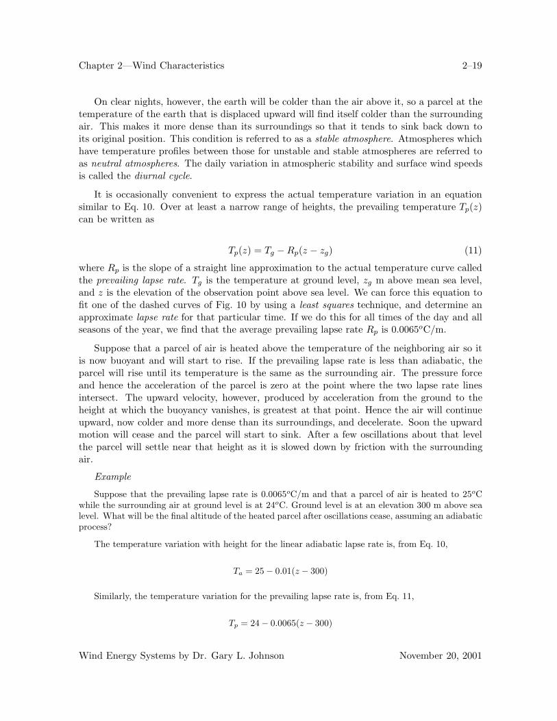
Suppose that the prevailing lapse rate is 0.0065oC/m and that a parcel of air is heated to 25oCwhile the surrounding air at ground level is at 24oC. Ground level is at an elevation 300 m above sealevel. What will be the final altitude of the heated parcel after oscillations cease, assuming an adiabaticprocess?
The temperature variation with height for the linear adiabatic lapse rate is, from Eq. 10,
Ta = 25 − 0.01(z − 300)
Similarly, the temperature variation for the prevailing lapse rate is, from Eq. 11,
Tp = 24 − 0.0065(z − 300)
Wind Energy Systems by Dr. Gary L. Johnson November 20, 2001
Chapter 2—Wind Characteristics 2–20
The two temperatures are the same at the point of equal buoyancy. Setting Ta equal to Tp andsolving for z yields an intersection height of about 585 m above sea level or 285 m above ground level.This is illustrated in Fig. 11.
Figure 11: Buoyancy of air in a stable atmosphere
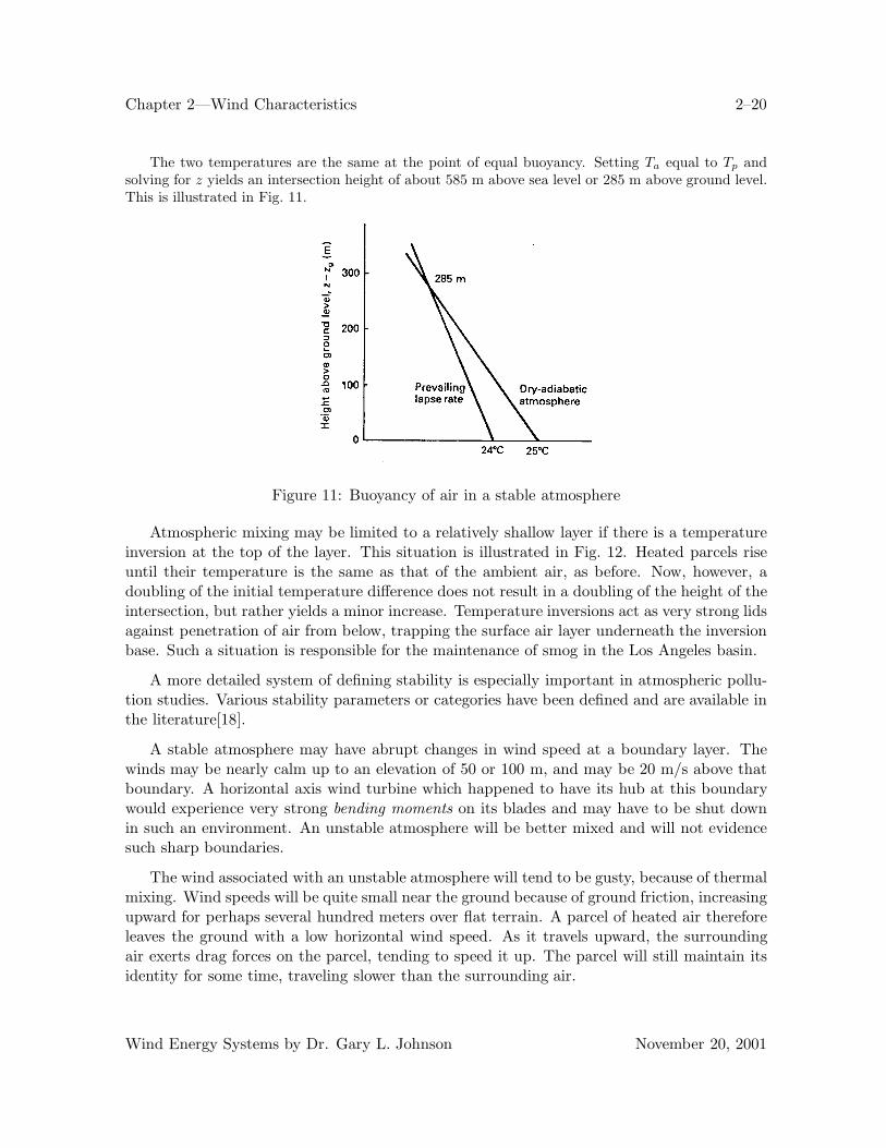
Atmospheric mixing may be limited to a relatively shallow layer if there is a temperatureinversion at the top of the layer. This situation is illustrated in Fig. 12. Heated parcels riseuntil their temperature is the same as that of the ambient air, as before. Now, however, adoubling of the initial temperature difference does not result in a doubling of the height of theintersection, but rather yields a minor increase. Temperature inversions act as very strong lidsagainst penetration of air from below, trapping the surface air layer underneath the inversionbase. Such a situation is responsible for the maintenance of smog in the Los Angeles basin.
A more detailed system of defining stability is especially important in atmospheric pollu-tion studies. Various stability parameters or categories have been defined and are available inthe literature[18].
A stable atmosphere may have abrupt changes in wind speed at a boundary layer. Thewinds may be nearly calm up to an elevation of 50 or 100 m, and may be 20 m/s above thatboundary. A horizontal axis wind turbine which happened to have its hub at this boundarywould experience very strong bending moments on its blades and may have to be shut downin such an environment. An unstable atmosphere will be better mixed and will not evidencesuch sharp boundaries.
The wind associated with an unstable atmosphere will tend to be gusty, because of thermalmixing. Wind speeds will be quite small near the ground because of ground friction, increasingupward for perhaps several hundred meters over flat terrain. A parcel of heated air thereforeleaves the ground with a low horizontal wind speed. As it travels upward, the surroundingair exerts drag forces on the parcel, tending to speed it up. The parcel will still maintain itsidentity for some time, traveling slower than the surrounding air.
Wind Energy Systems by Dr. Gary L. Johnson November 20, 2001
Chapter 2—Wind Characteristics 2–21
Figure 12: Deep buoyant layer topped by temperature inversion.
Parcels of air descending from above have higher horizontal speeds. They mix with theascending parcels, causing an observer near the ground to sense wind speeds both below andabove the mean wind speed. A parcel with higher velocity is called a gust, while a parcel withlower velocity is sometimes called a negative gust or a lull. These parcels vary widely in sizeand will hit a particular point in a random fashion. They are easily observed in the wavestructure of a lake or in a field of tall wheat.
Gusts pose a hazard to large wind turbines because of the sudden change in wind speedand direction experienced by the turbine during a gust. Vibrations may be established orstructural damage done. The wind turbine must be designed to withstand the peak gust thatit is likely to experience during its projected lifetime.
Gusts also pose a problem in the adjusting of the turbine blades during operation in thatthe sensing anemometer will experience a different wind speed from that experienced by theblades. A gust may hit the anemometer and cause the blade angle of attack (the angle at whichthe blade passes through the air) to be adjusted for a higher wind speed than the blades areactually experiencing. This will generally cause the power output to drop below the optimumamount. Conversely, when the sensing anemometer experiences a lull, the turbine may betrimmed (adjusted) to produce more than rated output because of the higher wind speed itis experiencing. These undesirable situations require the turbine control system to be rathercomplex, and to have long time constants. This means that the turbine will be aimed slightlyoff the instantaneous wind direction and not be optimally adjusted for the instantaneouswind speed a large fraction of the time. The power production of the turbine will therefore besomewhat lower than would be predicted for an optimally adjusted and aimed wind turbinein a steady wind. The amount of this reduction is difficult to measure or even to estimate,but could easily be on the order of a 10 % reduction. This makes the simpler vertical axismachines more competitive than they might appear from wind tunnel tests since they require
Wind Energy Systems by Dr. Gary L. Johnson November 20, 2001
Chapter 2—Wind Characteristics 2–22
no aiming or blade control.
Thus far, we have talked only about gusts due to thermal turbulence, which has a verystrong diurnal cycle. Gusts are also produced by mechanical turbulence, caused by higherspeed winds flowing over rough surfaces. When strong frontal systems pass through a region,the atmosphere will be mechanically mixed and little or no diurnal variation of wind speedwill be observed. When there is no significant mixing of the atmosphere due to either thermalor mechanical turbulence, a boundary layer may develop with relatively high speed laminarflow of air above the boundary and essentially calm conditions below it. Without the effectsof mixing, upper level wind speeds tend to be higher than when mixed with lower level winds.Thus it is quite possible for nighttime wind speeds to decrease near the ground and increasea few hundred meters above the ground. This phenomenon is called the nocturnal jet. Asmentioned earlier, most National Weather Service (NWS) anemometers have been locatedabout 10 m above the ground, so the height and frequency of occurrence of this nocturnal jethave not been well documented at many sites. Investigation of nocturnal jets is done eitherwith very tall towers (e.g. 200 m) or with meteorological balloons. Balloon data are notvery precise, as we shall see in more detail in the next chapter, but rather long term recordsare available of National Weather Service balloon launchings. When used with appropriatecaution, these data can show some very interesting variations of wind speed with height andtime of day.
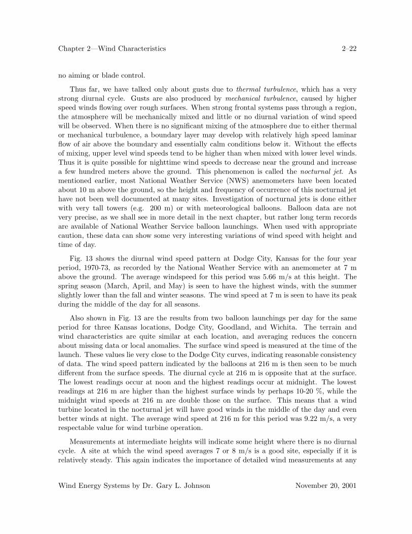
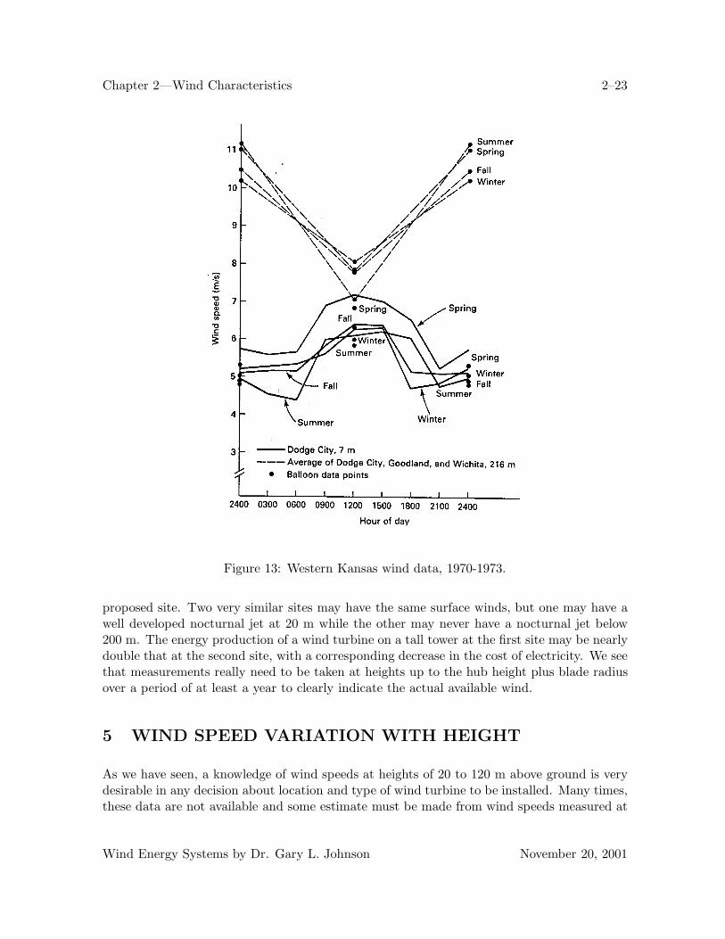
Fig. 13 shows the diurnal wind speed pattern at Dodge City, Kansas for the four yearperiod, 1970-73, as recorded by the National Weather Service with an anemometer at 7 mabove the ground. The average windspeed for this period was 5.66 m/s at this height. Thespring season (March, April, and May) is seen to have the highest winds, with the summerslightly lower than the fall and winter seasons. The wind speed at 7 m is seen to have its peakduring the middle of the day for all seasons.
Also shown in Fig. 13 are the results from two balloon launchings per day for the sameperiod for three Kansas locations, Dodge City, Goodland, and Wichita. The terrain andwind characteristics are quite similar at each location, and averaging reduces the concernabout missing data or local anomalies. The surface wind speed is measured at the time of thelaunch. These values lie very close to the Dodge City curves, indicating reasonable consistencyof data. The wind speed pattern indicated by the balloons at 216 m is then seen to be muchdifferent from the surface speeds. The diurnal cycle at 216 m is opposite that at the surface.The lowest readings occur at noon and the highest readings occur at midnight. The lowestreadings at 216 m are higher than the highest surface winds by perhaps 10-20 %, while themidnight wind speeds at 216 m are double those on the surface. This means that a windturbine located in the nocturnal jet will have good winds in the middle of the day and evenbetter winds at night. The average wind speed at 216 m for this period was 9.22 m/s, a veryrespectable value for wind turbine operation.
Measurements at intermediate heights will indicate some height where there is no diurnalcycle. A site at which the wind speed averages 7 or 8 m/s is a good site, especially if it isrelatively steady. This again indicates the importance of detailed wind measurements at any
Wind Energy Systems by Dr. Gary L. Johnson November 20, 2001
Chapter 2—Wind Characteristics 2–23
Figure 13: Western Kansas wind data, 1970-1973.
proposed site. Two very similar sites may have the same surface winds, but one may have awell developed nocturnal jet at 20 m while the other may never have a nocturnal jet below200 m. The energy production of a wind turbine on a tall tower at the first site may be nearlydouble that at the second site, with a corresponding decrease in the cost of electricity. We seethat measurements really need to be taken at heights up to the hub height plus blade radiusover a period of at least a year to clearly indicate the actual available wind.
5 WIND SPEED VARIATION WITH HEIGHT
As we have seen, a knowledge of wind speeds at heights of 20 to 120 m above ground is verydesirable in any decision about location and type of wind turbine to be installed. Many times,these data are not available and some estimate must be made from wind speeds measured at
Wind Energy Systems by Dr. Gary L. Johnson November 20, 2001
Chapter 2—Wind Characteristics 2–24
about 10 m. This requires an equation which predicts the wind speed at one height in termsof the measured speed at another, lower, height. Such equations are developed in texts onfluid mechanics. The derivations are beyond the scope of this text so we shall just use theresults. One possible form for the variation of wind speed u(z) with height z is
u(z) =uf
K
[ln
z
zo− ξ
(z
L
)](12)
Here uf is the friction velocity, K is the von Karman’s constant (normally assumed tobe 0.4), zo is the surface roughness length, and L is a scale factor called the Monin Obukovlength[17, 13]. The function ξ(z/L) is determined by the net solar radiation at the site. Thisequation applies to short term (e.g. 1 minute) average wind speeds, but not to monthly oryearly averages.
The surface roughness length zo will depend on both the size and the spacing of roughnesselements such as grass, crops, buildings, etc. Typical values of zo are about 0.01 cm for wateror snow surfaces, 1 cm for short grass, 25 cm for tall grass or crops, and 1 to 4 m for forestand city[19]. In practice, zo cannot be determined precisely from the appearance of a sitebut is determined from measurements of the wind. The same is true for the friction velocityuf , which is a function of surface friction and the air density, and ξ(z/L). The parametersare found by measuring the wind at three heights, writing Eq. 12 as three equations (one foreach height), and solving for the three unknowns uf , zo, and ξ(z/L). This is not a linearequation so nonlinear analysis must be used. The results must be classified by the directionof the wind and the time of year because zo varies with the upwind surface roughness and thecondition of the vegetation. Results must also be classified by the amount of net radiation sothe appropriate functional form of ξ(z/L) can be used.
All of this is quite satisfying for detailed studies on certain critical sites, but is too difficultto use for general engineering studies. This has led many people to look for simpler expressionswhich will yield satisfactory results even if they are not theoretically exact. The most commonof these simpler expressions is the power law, expressed as
u(z2)u(z1)
=(
z2
z1
)α
(13)
In this equation z1 is usually taken as the height of measurement, approximately 10 m,and z2 is the height at which a wind speed estimate is desired. The parameter α is determinedempirically. The equation can be made to fit observed wind data reasonably well over therange of 10 to perhaps 100 or 150 m if there are no sharp boundaries in the flow.
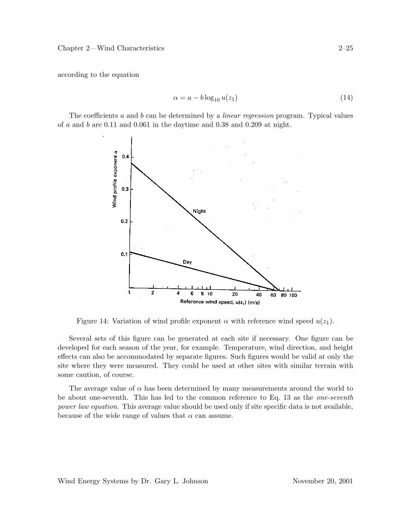
The exponent α varies with height, time of day, season of the year, nature of the terrain,wind speeds, and temperature[10]. A number of models have been proposed for the variationof α with these variables[22]. We shall use the linear logarithmic plot shown in Fig. 14.This figure shows one plot for day and another plot for night, each varying with wind speed
Wind Energy Systems by Dr. Gary L. Johnson November 20, 2001
Chapter 2—Wind Characteristics 2–25
according to the equation
α = a − b log10 u(z1) (14)
The coefficients a and b can be determined by a linear regression program. Typical valuesof a and b are 0.11 and 0.061 in the daytime and 0.38 and 0.209 at night.
Figure 14: Variation of wind profile exponent α with reference wind speed u(z1).
Several sets of this figure can be generated at each site if necessary. One figure can bedeveloped for each season of the year, for example. Temperature, wind direction, and heighteffects can also be accommodated by separate figures. Such figures would be valid at only thesite where they were measured. They could be used at other sites with similar terrain withsome caution, of course.
The average value of α has been determined by many measurements around the world tobe about one-seventh. This has led to the common reference to Eq. 13 as the one-seventhpower law equation. This average value should be used only if site specific data is not available,because of the wide range of values that α can assume.
Wind Energy Systems by Dr. Gary L. Johnson November 20, 2001

Chapter 2—Wind Characteristics 2–26
6 WIND-SPEED STATISTICS
The speed of the wind is continuously changing, making it desirable to describe the wind bystatistical methods. We shall pause here to examine a few of the basic concepts of probabilityand statistics, leaving a more detailed treatment to the many books written on the subject.
One statistical quantity which we have mentioned earlier is the average or arithmetic mean.If we have a set of numbers ui, such as a set of measured wind speeds, the mean of the set isdefined as
u =1n
n∑i=1
ui (15)
The sample size or the number of measured values is n.
Another quantity seen occasionally in the literature is the median. If n is odd, the medianis the middle number after all the numbers have been arranged in order of size. As manynumbers lie below the median as above it. If n is even the median is halfway between the twomiddle numbers when we rank the numbers.
In addition to the mean, we are interested in the variability of the set of numbers. Wewant to find the discrepancy or deviation of each number from the mean and then find somesort of average of these deviations. The mean of the deviations ui − u is zero, which does nottell us much. We therefore square each deviation to get all positive quantities. The varianceσ2 of the data is then defined as
σ2 =1
n − 1
n∑i=1
(ui − u)2 (16)
The term n - 1 is used rather than n for theoretical reasons we shall not discuss here[2].
The standard deviation σ is then defined as the square root of the variance.
standard deviation =√
variance (17)
Example
Five measured wind speeds are 2,4,7,8, and 9 m/s. Find the mean, the variance, and the standarddeviation.
u =15(2 + 4 + 7 + 8 + 9) = 6.00 m/s
Wind Energy Systems by Dr. Gary L. Johnson November 20, 2001
Chapter 2—Wind Characteristics 2–27
σ2 =14[(2 − 6)2 + (4 − 6)2 + (7 − 6)2 + (8 − 6)2 + (9 − 6)2]
=14(34) = 8.5 m2/s2
σ =√
8.5 = 2.92 m/s
Wind speeds are normally measured in integer values, so that each integer value is observedmany times during a year of observations. The numbers of observations of a specific windspeed ui will be defined as mi. The mean is then
u =1n
w∑i=1
miui (18)
where w is the number of different values of wind speed observed and n is still the totalnumber of observations.
It can be shown[2] that the variance is given by
σ2 =1
n − 1
w∑
i=1
miu2i −
1n
(w∑
i=1
miui
)2 (19)
The two terms inside the brackets are nearly equal to each other so full precision needs to bemaintained during the computation. This is not difficult with most of the hand calculatorsthat are available.
Example
A wind data acquisition system located in the tradewinds on the northeast coast of Puerto Ricomeasures 6 m/s 19 times, 7 m/s 54 times, and 8 m/s 42 times during a given period. Find the mean,variance, and standard deviation.
u =1
115[19(6) + 54(7) + 42(8)] = 7.20 m/s
σ2 = { 1114
[19(6)2 + 54(7)2 + 42(8)2 − 1115
[19(6) + 54(7) + 42(8)]2}
=1
114(6018− 5961.600) = 0.495 m2/s2
σ = 0.703 m/s
Wind Energy Systems by Dr. Gary L. Johnson November 20, 2001
Chapter 2—Wind Characteristics 2–28
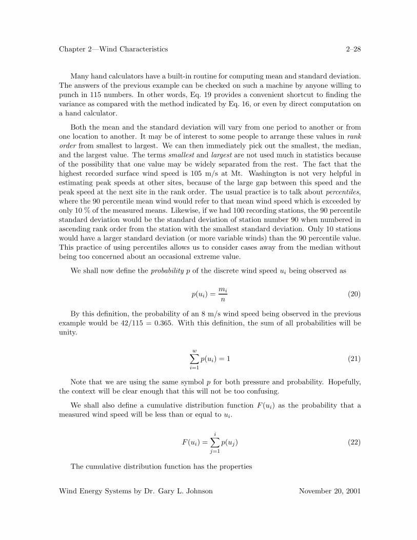
Many hand calculators have a built-in routine for computing mean and standard deviation.The answers of the previous example can be checked on such a machine by anyone willing topunch in 115 numbers. In other words, Eq. 19 provides a convenient shortcut to finding thevariance as compared with the method indicated by Eq. 16, or even by direct computation ona hand calculator.
Both the mean and the standard deviation will vary from one period to another or fromone location to another. It may be of interest to some people to arrange these values in rankorder from smallest to largest. We can then immediately pick out the smallest, the median,and the largest value. The terms smallest and largest are not used much in statistics becauseof the possibility that one value may be widely separated from the rest. The fact that thehighest recorded surface wind speed is 105 m/s at Mt. Washington is not very helpful inestimating peak speeds at other sites, because of the large gap between this speed and thepeak speed at the next site in the rank order. The usual practice is to talk about percentiles,where the 90 percentile mean wind would refer to that mean wind speed which is exceeded byonly 10 % of the measured means. Likewise, if we had 100 recording stations, the 90 percentilestandard deviation would be the standard deviation of station number 90 when numbered inascending rank order from the station with the smallest standard deviation. Only 10 stationswould have a larger standard deviation (or more variable winds) than the 90 percentile value.This practice of using percentiles allows us to consider cases away from the median withoutbeing too concerned about an occasional extreme value.
We shall now define the probability p of the discrete wind speed ui being observed as
p(ui) =mi
n(20)
By this definition, the probability of an 8 m/s wind speed being observed in the previousexample would be 42/115 = 0.365. With this definition, the sum of all probabilities will beunity.
w∑i=1
p(ui) = 1 (21)
Note that we are using the same symbol p for both pressure and probability. Hopefully,the context will be clear enough that this will not be too confusing.
We shall also define a cumulative distribution function F (ui) as the probability that ameasured wind speed will be less than or equal to ui.
F (ui) =i∑
j=1
p(uj) (22)
The cumulative distribution function has the properties
Wind Energy Systems by Dr. Gary L. Johnson November 20, 2001
Chapter 2—Wind Characteristics 2–29
F (−∞) = 0, F (∞) = 1 (23)
Example
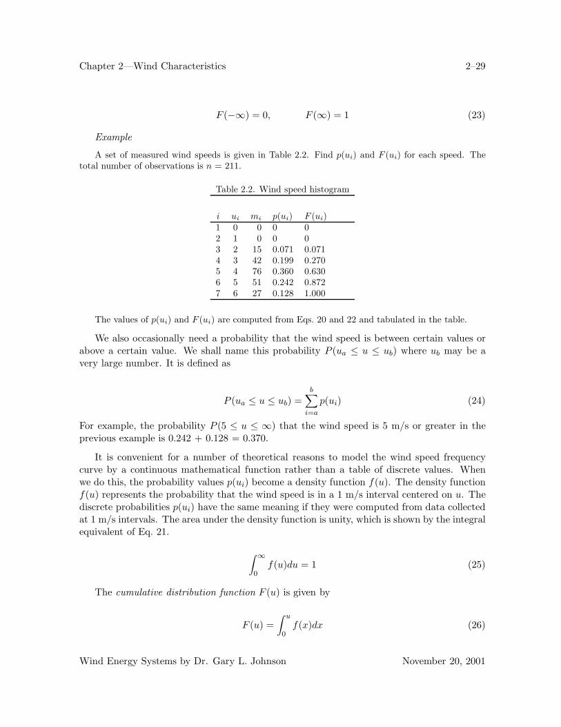
A set of measured wind speeds is given in Table 2.2. Find p(ui) and F (ui) for each speed. Thetotal number of observations is n = 211.
Table 2.2. Wind speed histogram
i ui mi p(ui) F (ui)1 0 0 0 02 1 0 0 03 2 15 0.071 0.0714 3 42 0.199 0.2705 4 76 0.360 0.6306 5 51 0.242 0.8727 6 27 0.128 1.000
The values of p(ui) and F (ui) are computed from Eqs. 20 and 22 and tabulated in the table.
We also occasionally need a probability that the wind speed is between certain values orabove a certain value. We shall name this probability P (ua ≤ u ≤ ub) where ub may be avery large number. It is defined as
P (ua ≤ u ≤ ub) =b∑
i=a
p(ui) (24)
For example, the probability P (5 ≤ u ≤ ∞) that the wind speed is 5 m/s or greater in theprevious example is 0.242 + 0.128 = 0.370.
It is convenient for a number of theoretical reasons to model the wind speed frequencycurve by a continuous mathematical function rather than a table of discrete values. Whenwe do this, the probability values p(ui) become a density function f(u). The density functionf(u) represents the probability that the wind speed is in a 1 m/s interval centered on u. Thediscrete probabilities p(ui) have the same meaning if they were computed from data collectedat 1 m/s intervals. The area under the density function is unity, which is shown by the integralequivalent of Eq. 21.
∫ ∞
0f(u)du = 1 (25)
The cumulative distribution function F (u) is given by
F (u) =∫ u
0f(x)dx (26)
Wind Energy Systems by Dr. Gary L. Johnson November 20, 2001
Chapter 2—Wind Characteristics 2–30
The variable x inside the integral is just a dummy variable representing wind speed forthe purpose of integration.
Both of the above integrations start at zero because the wind speed cannot be negative.When the wind speed is considered as a continuous random variable, the cumulative distri-bution function has the properties F (0) = 0 and F (∞) = 1. The quantity F (0) will notnecessarily be zero in the discrete case because there will normally be some zero wind speedsmeasured which are included in F (0). In the continuous case, however, F (0) is the integral ofEq. 26 with integration limits both starting and ending at zero. Since f(u) is a well behavedfunction at u = 0, the integration has to yield a result of zero. This is a minor technical pointwhich should not cause any difficulties later.
We will sometimes need the inverse of Eq. 26 for computational purposes. This is givenby
f(u) =dF (u)
du(27)
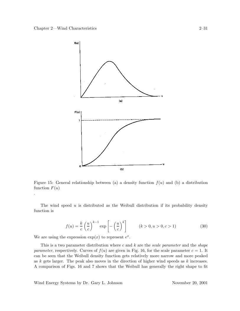
The general relationship between f(u) and F (u) is sketched in Fig. 15. F (u) starts at 0,changes most rapidly at the peak of f(u), and approaches 1 asymptotically.
The mean value of the density function f(u) is given by
u =∫ ∞
0uf(u)du (28)
The variance is given by
σ2 =∫ ∞
0(u − u)2f(u)du (29)
These equations are used to compute theoretical values of mean and variance for a widevariety of statistical functions that are used in various applications.
7 WEIBULL STATISTICS
There are several density functions which can be used to describe the wind speed frequencycurve. The two most common are the Weibull and the Rayleigh functions. For the statisticallyinclined reader, the Weibull is a special case of the Pearson Type III or generalized gammadistribution, while the Rayleigh [or chi with two degrees of freedom(chi-2)] distribution is asubset of the Weibull. The Weibull is a two parameter distribution while the Rayleigh has onlyone parameter. This makes the Weibull somewhat more versatile and the Rayleigh somewhatsimpler to use. We shall present the Weibull distribution first.
Wind Energy Systems by Dr. Gary L. Johnson November 20, 2001
Chapter 2—Wind Characteristics 2–31
Figure 15: General relationship between (a) a density function f(u) and (b) a distributionfunction F (u).
The wind speed u is distributed as the Weibull distribution if its probability densityfunction is
f(u) =k
c
(u
c
)k−1
exp
[−(
u
c
)k]
(k > 0, u > 0, c > 1) (30)
We are using the expression exp(x) to represent ex.
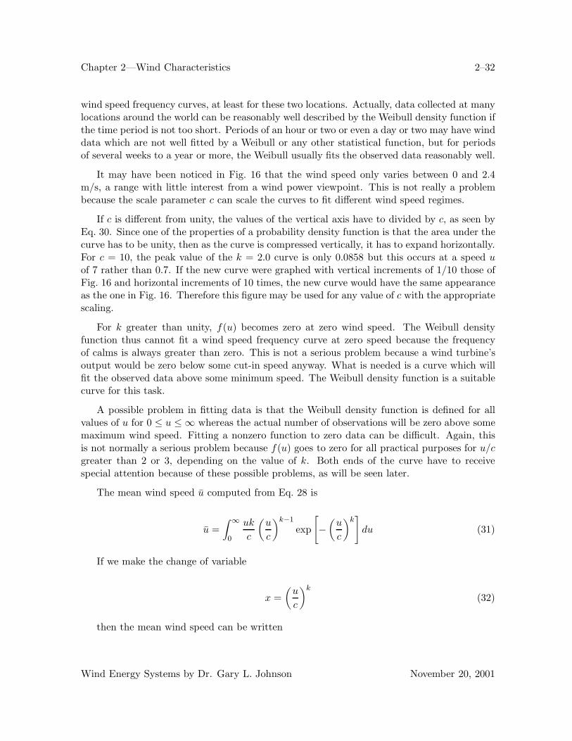
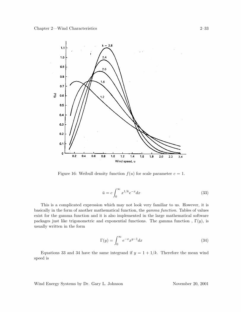
This is a two parameter distribution where c and k are the scale parameter and the shapeparameter, respectively. Curves of f(u) are given in Fig. 16, for the scale parameter c = 1. Itcan be seen that the Weibull density function gets relatively more narrow and more peakedas k gets larger. The peak also moves in the direction of higher wind speeds as k increases.A comparison of Figs. 16 and 7 shows that the Weibull has generally the right shape to fit
Wind Energy Systems by Dr. Gary L. Johnson November 20, 2001
Chapter 2—Wind Characteristics 2–32
wind speed frequency curves, at least for these two locations. Actually, data collected at manylocations around the world can be reasonably well described by the Weibull density function ifthe time period is not too short. Periods of an hour or two or even a day or two may have winddata which are not well fitted by a Weibull or any other statistical function, but for periodsof several weeks to a year or more, the Weibull usually fits the observed data reasonably well.
It may have been noticed in Fig. 16 that the wind speed only varies between 0 and 2.4m/s, a range with little interest from a wind power viewpoint. This is not really a problembecause the scale parameter c can scale the curves to fit different wind speed regimes.
If c is different from unity, the values of the vertical axis have to divided by c, as seen byEq. 30. Since one of the properties of a probability density function is that the area under thecurve has to be unity, then as the curve is compressed vertically, it has to expand horizontally.For c = 10, the peak value of the k = 2.0 curve is only 0.0858 but this occurs at a speed uof 7 rather than 0.7. If the new curve were graphed with vertical increments of 1/10 those ofFig. 16 and horizontal increments of 10 times, the new curve would have the same appearanceas the one in Fig. 16. Therefore this figure may be used for any value of c with the appropriatescaling.
For k greater than unity, f(u) becomes zero at zero wind speed. The Weibull densityfunction thus cannot fit a wind speed frequency curve at zero speed because the frequencyof calms is always greater than zero. This is not a serious problem because a wind turbine’soutput would be zero below some cut-in speed anyway. What is needed is a curve which willfit the observed data above some minimum speed. The Weibull density function is a suitablecurve for this task.
A possible problem in fitting data is that the Weibull density function is defined for allvalues of u for 0 ≤ u ≤ ∞ whereas the actual number of observations will be zero above somemaximum wind speed. Fitting a nonzero function to zero data can be difficult. Again, thisis not normally a serious problem because f(u) goes to zero for all practical purposes for u/cgreater than 2 or 3, depending on the value of k. Both ends of the curve have to receivespecial attention because of these possible problems, as will be seen later.
The mean wind speed u computed from Eq. 28 is
u =∫ ∞
0
uk
c
(u
c
)k−1
exp
[−(
u
c
)k]
du (31)
If we make the change of variable
x =(
u
c
)k
(32)
then the mean wind speed can be written
Wind Energy Systems by Dr. Gary L. Johnson November 20, 2001
Chapter 2—Wind Characteristics 2–33
Figure 16: Weibull density function f(u) for scale parameter c = 1.
u = c
∫ ∞
0x1/ke−xdx (33)
This is a complicated expression which may not look very familiar to us. However, it isbasically in the form of another mathematical function, the gamma function. Tables of valuesexist for the gamma function and it is also implemented in the large mathematical softwarepackages just like trigonometric and exponential functions. The gamma function , Γ(y), isusually written in the form
Γ(y) =∫ ∞
0e−xxy−1dx (34)
Equations 33 and 34 have the same integrand if y = 1 + 1/k. Therefore the mean windspeed is
Wind Energy Systems by Dr. Gary L. Johnson November 20, 2001
Chapter 2—Wind Characteristics 2–34
u = cΓ(
1 +1k
)(35)
Published tables that are available for the gamma function Γ(y) are only given for 1 ≤ y ≤ 2.If an argument y lies outside this range, the recursive relation
Γ(y + 1) = yΓ(y) (36)
must be used. If y is an integer,
Γ(y + 1) = y! = y(y − 1)(y − 2) · · · (1) (37)
The factorial y! is implemented on the more powerful hand calculators. The argument yis not restricted to an integer, so the quantity computed is actually Γ(y + 1). This may bethe most convenient way of calculating the gamma function in many situations.
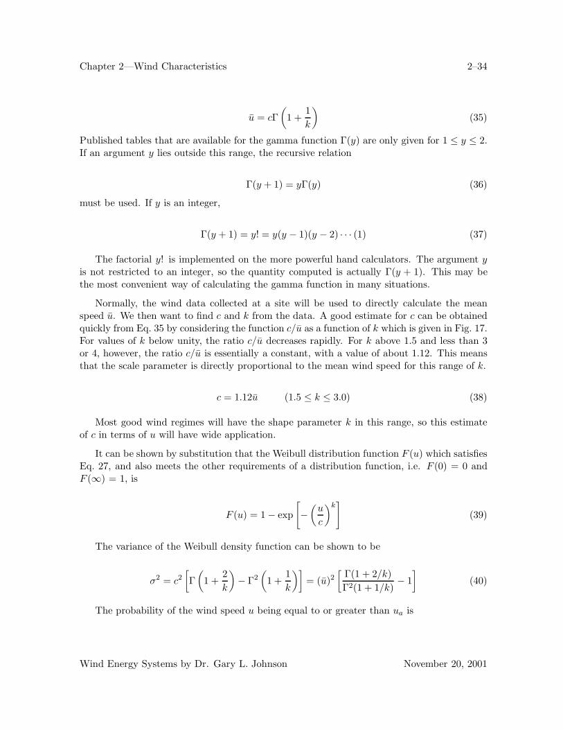
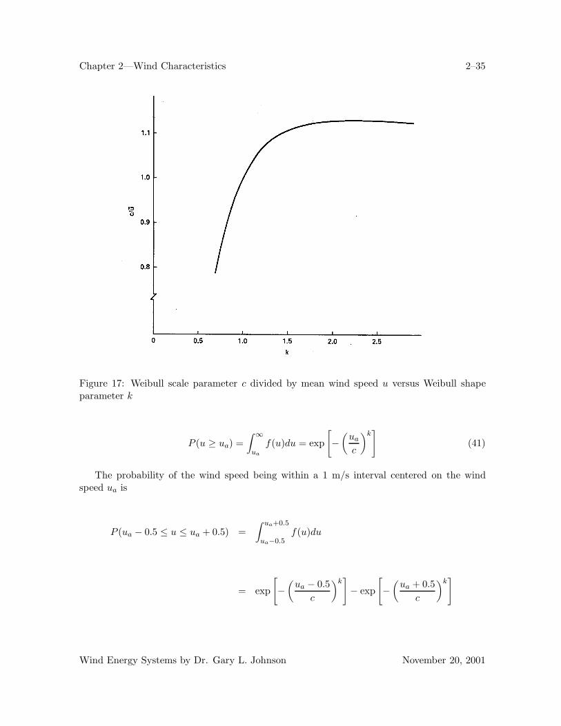
Normally, the wind data collected at a site will be used to directly calculate the meanspeed u. We then want to find c and k from the data. A good estimate for c can be obtainedquickly from Eq. 35 by considering the function c/u as a function of k which is given in Fig. 17.For values of k below unity, the ratio c/u decreases rapidly. For k above 1.5 and less than 3or 4, however, the ratio c/u is essentially a constant, with a value of about 1.12. This meansthat the scale parameter is directly proportional to the mean wind speed for this range of k.
c = 1.12u (1.5 ≤ k ≤ 3.0) (38)
Most good wind regimes will have the shape parameter k in this range, so this estimateof c in terms of u will have wide application.
It can be shown by substitution that the Weibull distribution function F (u) which satisfiesEq. 27, and also meets the other requirements of a distribution function, i.e. F (0) = 0 andF (∞) = 1, is
F (u) = 1 − exp
[−(
u
c
)k]
(39)
The variance of the Weibull density function can be shown to be
σ2 = c2[Γ(
1 +2k
)− Γ2
(1 +
1k
)]= (u)2
[Γ(1 + 2/k)Γ2(1 + 1/k)
− 1]
(40)
The probability of the wind speed u being equal to or greater than ua is
Wind Energy Systems by Dr. Gary L. Johnson November 20, 2001
Chapter 2—Wind Characteristics 2–35
Figure 17: Weibull scale parameter c divided by mean wind speed u versus Weibull shapeparameter k
P (u ≥ ua) =∫ ∞
ua
f(u)du = exp
[−(
ua
c
)k]
(41)
The probability of the wind speed being within a 1 m/s interval centered on the windspeed ua is
P (ua − 0.5 ≤ u ≤ ua + 0.5) =∫ ua+0.5
ua−0.5f(u)du
= exp
[−(
ua − 0.5c
)k]− exp
[−(
ua + 0.5c
)k]
Wind Energy Systems by Dr. Gary L. Johnson November 20, 2001
Chapter 2—Wind Characteristics 2–36
� f(ua)∆u = f(ua) (42)
Example
The Weibull parameters at a given site are c = 6 m/s and k = 1.8. Estimate the number of hoursper year that the wind speed will be between 6.5 and 7.5 m/s. Estimate the number of hours per yearthat the wind speed is greater than or equal to 15 m/s.
From Eq. 42, the probability that the wind is between 6.5 and 7.5 m/s is just f(7), which can beevaluated from Eq. 30 as
f(7) =1.86
(76
)1.8−1
exp
[−(
76
)1.8]
= 0.0907
This means that the wind speed will be in this interval 9.07 % of the time, so the number of hours peryear with wind speeds in this interval would be
(0.0907)(8760) = 794 h/year
From Eq. 41, the probability that the wind speed is greater than or equal to 15 m/s is
P (u ≥ 15) = exp
[−(
156
)1.8]
= 0.0055
which represents
(0.0055)(8760) = 48 h/year
If a particular wind turbine had to be shut down in wind speeds above 15 m/s, about 2days per year of operating time would be lost.
We shall see in Chapter 4 that the power in the wind passing through an area A perpen-dicular to the wind is given by
Pw =12ρAu3 W (43)
The average power in the wind is then
Pw =12ρA
w∑i=1
p(ui)u3i W (44)
Wind Energy Systems by Dr. Gary L. Johnson November 20, 2001
Chapter 2—Wind Characteristics 2–37
We may think of this value as the true or actual power in the wind if the probabilitiesp(ui) are determined from the actual wind speed data.
If we model the actual wind data by a probability density function f(u), then the averagepower in the wind is
Pw =12ρA
∫ ∞
0u3f(u)du W (45)
It can be shown[13] that when f(u) is the Weibull density function, the average power is
Pw =ρAu3Γ(1 + 3/k)2[Γ(1 + 1/k)]3
W (46)
If the Weibull density function fits the actual wind data exactly, then the power in thewind predicted by Eq. 46 will be the same as that predicted by Eq. 44. The greater thedifference between the values obtained from these two equations, the poorer is the fit of theWeibull density function to the actual data.
Actually, wind speeds outside some range are of little use to a practical wind turbine.There is inadequate power to spin the turbine below perhaps 5 or 6 m/s and the turbine mayreach its rated power at 12 m/s. Excess wind power is spilled or wasted above this speed sothe turbine output power can be maintained at a constant value. Therefore, the quality of fitbetween the actual data and the Weibull model is more important within this range than overall wind speeds. We shall consider some numerical examples of these fits later in the chapter.
The function u3f(u) starts at zero at u = 0, reaches a peak value at some wind speedume, and finally returns to zero at large values of u. The yearly energy production at windspeed ui is the power in the wind times the fraction of time that power is observed times thenumber of hours in the year. The wind speed ume is the speed which produces more energy(the product of power and time) than any other wind speed. Therefore, the maximum energyobtained from any one wind speed is
Wmax =12ρAu3
mef(ume)(8760) (47)
The turbine should be designed so this wind speed with maximum energy content isincluded in its best operating wind speed range. Some applications will even require theturbine to be designed with a rated wind speed equal to this maximum energy wind speed.We therefore want to find the wind speed ume. This can be found by multiplying Eq. eq:2.30by u3, setting the derivative equal to zero, and solving for u. After a moderate amount ofalgebra the result can be shown to be
ume = c
(k + 2
k
)1/k
m/s (48)
Wind Energy Systems by Dr. Gary L. Johnson November 20, 2001
Chapter 2—Wind Characteristics 2–38
We see that ume is greater than c so it will therefore be greater than the mean speed u. Ifthe mean speed is 6 m/s, then ume will typically be about 8 or 9 m/s.
We see that a number of interesting results can be obtained by modeling the wind speedhistogram by a Weibull density function. Other results applicable to the power output of windturbines are developed in Chapter 4.
8 DETERMINING THE WEIBULL PARAMETERS
There are several methods available for determining the Weibull parameters c and k[13]. Ifthe mean and variance of the wind speed are known, then Eqs. 35 and 40 can be solved for cand k directly. At first glance, this would seem impossible because k is buried in the argumentof a gamma function. However, Justus[13] has determined that an acceptable approximationfor k from Eq. 40 is
k =(
σ
u
)−1.086
(49)
This is a reasonably good approximation over the range 1 ≤k≤ 10. Once k has beendetermined, Eq. 35 can be solved for c.
c =u
Γ(1 + 1/k)(50)
The variance of a histogram of wind speeds is not difficult to find from Eq. 19, so thismethod yields the parameters c and k rather easily. The method can even be used whenthe variance is not known, by simply estimating k. Justus[13] examined the wind speeddistributions at 140 sites across the continental United States measured at heights near 10 m,and found that k appears to be proportional to the square root of the mean wind speed.
k = d1
√u (51)
The proportionality constant d1 is a site specific constant with an average value of 0.94when the mean wind speed u is given in meters per second. The constant d1 is between 0.73and 1.05 for 80 % of the sites. The average value of d1 is normally adequate for wind powercalculations, but if more accuracy is desired, several months of wind data can be collected andanalyzed in more detail to compute c and k. These values of k can be plotted versus
√u on
log-log paper, a line drawn through the points, and d1 determined from the slope of the line.
Another method of determining c and k which lends itself to computer analysis, is the leastsquares approximation to a straight line. That is, we perform the necessary mathematicaloperations on Eq. 30 to linearize it and then determine c and k to minimize the least squared
Wind Energy Systems by Dr. Gary L. Johnson November 20, 2001
Chapter 2—Wind Characteristics 2–39
error between the linearized ideal curve and the actual data points of p(ui). The process issomewhat of an art and there may be more than one procedure which will yield a satisfactoryresult. Whether the result is satisfactory or not has to be judged by the agreement betweenthe Weibull curve and the raw data, particularly as it is used in wind power computations.
The first step of linearization is to integrate Eq. 27. This yields the distribution functionF (u) which is given by Eq. 39. As can be seen in Fig. 15, F (u) is more nearly describable by astraight line than f(u), but is still quite nonlinear. We note that F (u) contains an exponentialand that, in general, exponentials are linearized by taking the logarithm. In this case, becausethe exponent is itself raised to a power, we must take logarithms twice.
ln[− ln(1 − F (u))] = k ln u − k ln c (52)
This is in the form of an equation of a straight line
y = ax + b (53)
where x and y are variables, a is the slope, and b is the intercept of the line on the y axis. Inparticular,
y = ln[− ln(1 − F (u)]a = k (54)x = lnu
b = −k ln c
Data will be expressed in the form of pairs of values of ui and F (ui). For each wind speedui there is a corresponding value of the cumulative distribution function F (ui). When givenvalues for u = ui and F (u) = F (ui) we can find values for x = xi and y = yi in Eqs. 55. Beingactual data, these pairs of values do not fall exactly on a straight line, of course. The ideais to determine the values of a and b in Eq. 53 such that a straight line drawn through thesepoints has the best possible fit. It can be shown that the proper values for a and b are
a =
w∑i=1
xiyi −
w∑i=1
xi
w∑i=1
yi
w
w∑i=1
x2i −
( w∑i=1
xi
)2
w
=
w∑i=1
(xi − x)(yi − y)
w∑i=1
(xi − x)2(55)
b = yi − axi =1w
w∑i=1
yi − a
w
w∑i=1
xi (56)
Wind Energy Systems by Dr. Gary L. Johnson November 20, 2001
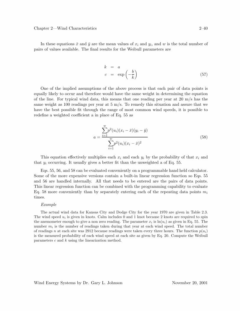
Chapter 2—Wind Characteristics 2–40
In these equations x and y are the mean values of xi and yi, and w is the total number ofpairs of values available. The final results for the Weibull parameters are
k = a
c = exp(− b
k
)(57)
One of the implied assumptions of the above process is that each pair of data points isequally likely to occur and therefore would have the same weight in determining the equationof the line. For typical wind data, this means that one reading per year at 20 m/s has thesame weight as 100 readings per year at 5 m/s. To remedy this situation and assure that wehave the best possible fit through the range of most common wind speeds, it is possible toredefine a weighted coefficient a in place of Eq. 55 as
a =
w∑i=1
p2(ui)(xi − x)(yi − y)
w∑i=1
p2(ui)(xi − x)2(58)
This equation effectively multiplies each xi and each yi by the probability of that xi andthat yi occurring. It usually gives a better fit than the unweighted a of Eq. 55.
Eqs. 55, 56, and 58 can be evaluated conveniently on a programmable hand held calculator.Some of the more expensive versions contain a built-in linear regression function so Eqs. 55and 56 are handled internally. All that needs to be entered are the pairs of data points.This linear regression function can be combined with the programming capability to evaluateEq. 58 more conveniently than by separately entering each of the repeating data points mi
times.
Example
The actual wind data for Kansas City and Dodge City for the year 1970 are given in Table 2.3.The wind speed ui is given in knots. Calm includes 0 and 1 knot because 2 knots are required to spinthe anemometer enough to give a non zero reading. The parameter xi is ln(ui) as given in Eq. 55. Thenumber mi is the number of readings taken during that year at each wind speed. The total numberof readings n at each site was 2912 because readings were taken every three hours. The function p(ui)is the measured probability of each wind speed at each site as given by Eq. 20. Compute the Weibullparameters c and k using the linearization method.
Wind Energy Systems by Dr. Gary L. Johnson November 20, 2001
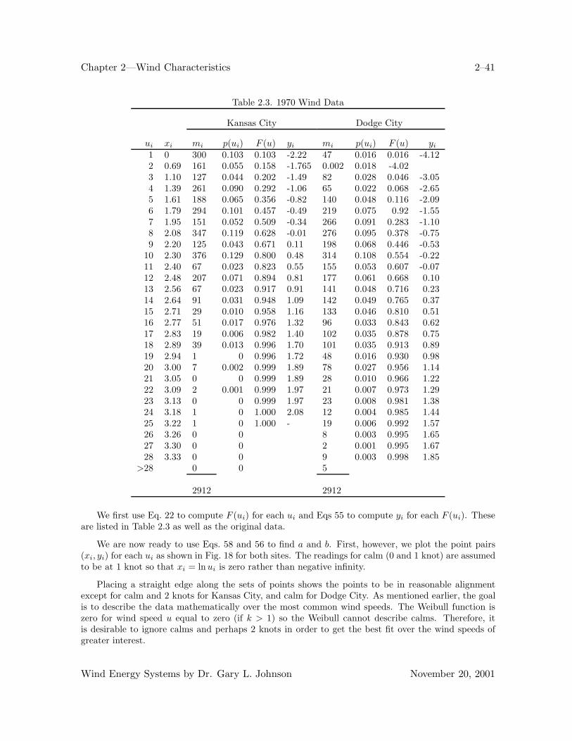
Chapter 2—Wind Characteristics 2–41
Table 2.3. 1970 Wind Data
Kansas City Dodge City
ui xi mi p(ui) F (u) yi mi p(ui) F (u) yi
1 0 300 0.103 0.103 -2.22 47 0.016 0.016 -4.122 0.69 161 0.055 0.158 -1.765 0.002 0.018 -4.023 1.10 127 0.044 0.202 -1.49 82 0.028 0.046 -3.054 1.39 261 0.090 0.292 -1.06 65 0.022 0.068 -2.655 1.61 188 0.065 0.356 -0.82 140 0.048 0.116 -2.096 1.79 294 0.101 0.457 -0.49 219 0.075 0.92 -1.557 1.95 151 0.052 0.509 -0.34 266 0.091 0.283 -1.108 2.08 347 0.119 0.628 -0.01 276 0.095 0.378 -0.759 2.20 125 0.043 0.671 0.11 198 0.068 0.446 -0.53
10 2.30 376 0.129 0.800 0.48 314 0.108 0.554 -0.2211 2.40 67 0.023 0.823 0.55 155 0.053 0.607 -0.0712 2.48 207 0.071 0.894 0.81 177 0.061 0.668 0.1013 2.56 67 0.023 0.917 0.91 141 0.048 0.716 0.2314 2.64 91 0.031 0.948 1.09 142 0.049 0.765 0.3715 2.71 29 0.010 0.958 1.16 133 0.046 0.810 0.5116 2.77 51 0.017 0.976 1.32 96 0.033 0.843 0.6217 2.83 19 0.006 0.982 1.40 102 0.035 0.878 0.7518 2.89 39 0.013 0.996 1.70 101 0.035 0.913 0.8919 2.94 1 0 0.996 1.72 48 0.016 0.930 0.9820 3.00 7 0.002 0.999 1.89 78 0.027 0.956 1.1421 3.05 0 0 0.999 1.89 28 0.010 0.966 1.2222 3.09 2 0.001 0.999 1.97 21 0.007 0.973 1.2923 3.13 0 0 0.999 1.97 23 0.008 0.981 1.3824 3.18 1 0 1.000 2.08 12 0.004 0.985 1.4425 3.22 1 0 1.000 - 19 0.006 0.992 1.5726 3.26 0 0 8 0.003 0.995 1.6527 3.30 0 0 2 0.001 0.995 1.6728 3.33 0 0 9 0.003 0.998 1.85
>28 0 0 5
2912 2912
We first use Eq. 22 to compute F (ui) for each ui and Eqs 55 to compute yi for each F (ui). Theseare listed in Table 2.3 as well as the original data.
We are now ready to use Eqs. 58 and 56 to find a and b. First, however, we plot the point pairs(xi, yi) for each ui as shown in Fig. 18 for both sites. The readings for calm (0 and 1 knot) are assumedto be at 1 knot so that xi = ln ui is zero rather than negative infinity.
Placing a straight edge along the sets of points shows the points to be in reasonable alignmentexcept for calm and 2 knots for Kansas City, and calm for Dodge City. As mentioned earlier, the goalis to describe the data mathematically over the most common wind speeds. The Weibull function iszero for wind speed u equal to zero (if k > 1) so the Weibull cannot describe calms. Therefore, itis desirable to ignore calms and perhaps 2 knots in order to get the best fit over the wind speeds ofgreater interest.
Wind Energy Systems by Dr. Gary L. Johnson November 20, 2001
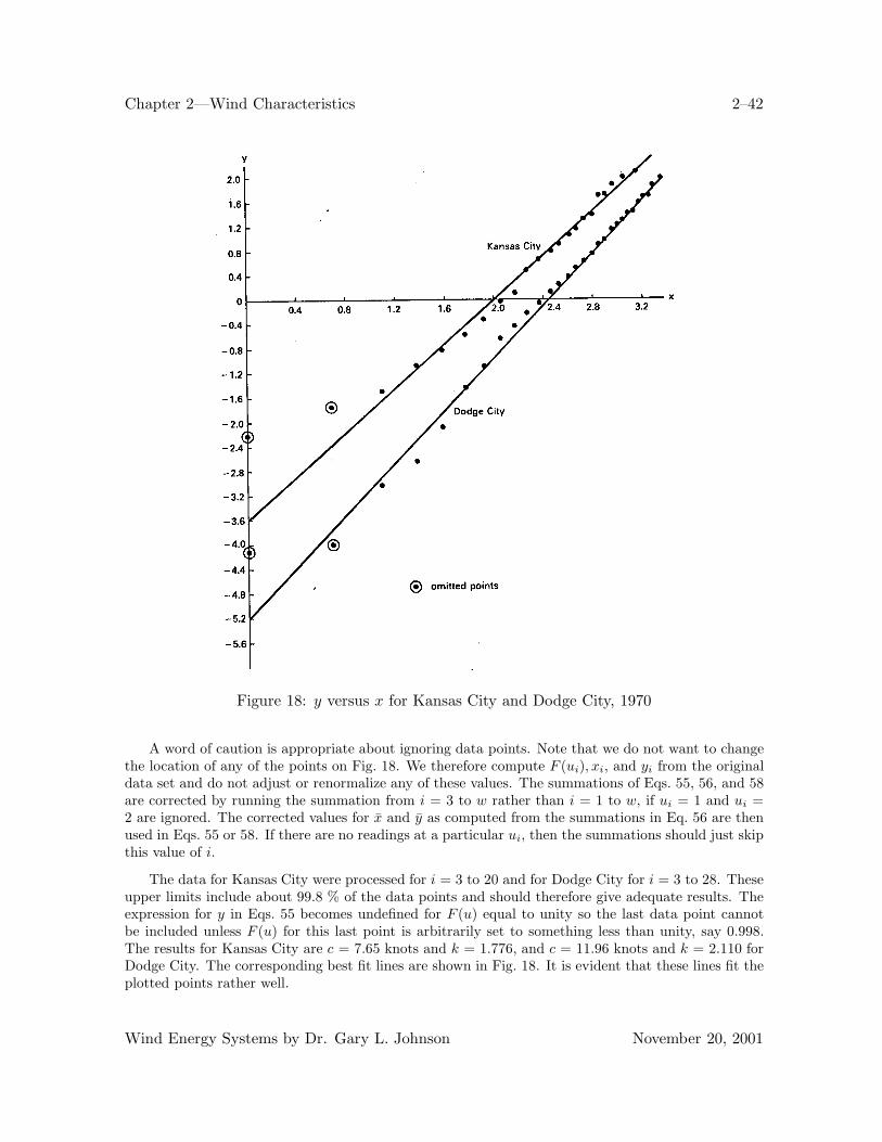
Chapter 2—Wind Characteristics 2–42
Figure 18: y versus x for Kansas City and Dodge City, 1970
A word of caution is appropriate about ignoring data points. Note that we do not want to changethe location of any of the points on Fig. 18. We therefore compute F (ui), xi, and yi from the originaldata set and do not adjust or renormalize any of these values. The summations of Eqs. 55, 56, and 58are corrected by running the summation from i = 3 to w rather than i = 1 to w, if ui = 1 and ui =2 are ignored. The corrected values for x and y as computed from the summations in Eq. 56 are thenused in Eqs. 55 or 58. If there are no readings at a particular ui, then the summations should just skipthis value of i.
The data for Kansas City were processed for i = 3 to 20 and for Dodge City for i = 3 to 28. Theseupper limits include about 99.8 % of the data points and should therefore give adequate results. Theexpression for y in Eqs. 55 becomes undefined for F (u) equal to unity so the last data point cannotbe included unless F (u) for this last point is arbitrarily set to something less than unity, say 0.998.The results for Kansas City are c = 7.65 knots and k = 1.776, and c = 11.96 knots and k = 2.110 forDodge City. The corresponding best fit lines are shown in Fig. 18. It is evident that these lines fit theplotted points rather well.
Wind Energy Systems by Dr. Gary L. Johnson November 20, 2001
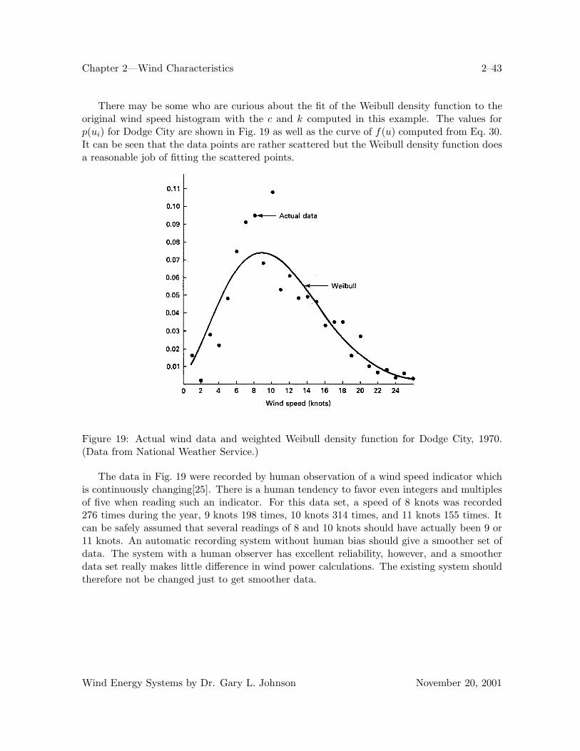
Chapter 2—Wind Characteristics 2–43
There may be some who are curious about the fit of the Weibull density function to theoriginal wind speed histogram with the c and k computed in this example. The values forp(ui) for Dodge City are shown in Fig. 19 as well as the curve of f(u) computed from Eq. 30.It can be seen that the data points are rather scattered but the Weibull density function doesa reasonable job of fitting the scattered points.
Figure 19: Actual wind data and weighted Weibull density function for Dodge City, 1970.(Data from National Weather Service.)
The data in Fig. 19 were recorded by human observation of a wind speed indicator whichis continuously changing[25]. There is a human tendency to favor even integers and multiplesof five when reading such an indicator. For this data set, a speed of 8 knots was recorded276 times during the year, 9 knots 198 times, 10 knots 314 times, and 11 knots 155 times. Itcan be safely assumed that several readings of 8 and 10 knots should have actually been 9 or11 knots. An automatic recording system without human bias should give a smoother set ofdata. The system with a human observer has excellent reliability, however, and a smootherdata set really makes little difference in wind power calculations. The existing system shouldtherefore not be changed just to get smoother data.
Wind Energy Systems by Dr. Gary L. Johnson November 20, 2001
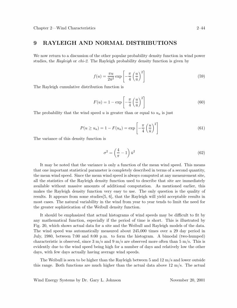
Chapter 2—Wind Characteristics 2–44
9 RAYLEIGH AND NORMAL DISTRIBUTIONS
We now return to a discussion of the other popular probability density function in wind powerstudies, the Rayleigh or chi-2. The Rayleigh probability density function is given by
f(u) =πu
2u2exp
[−π
4
(u
u
)2]
(59)
The Rayleigh cumulative distribution function is
F (u) = 1 − exp
[−π
4
(u
u
)2]
(60)
The probability that the wind speed u is greater than or equal to ua is just
P (u ≥ ua) = 1 − F (ua) = exp
[−π
4
(u
u
)2]
(61)
The variance of this density function is
σ2 =(
4π− 1
)u2 (62)
It may be noted that the variance is only a function of the mean wind speed. This meansthat one important statistical parameter is completely described in terms of a second quantity,the mean wind speed. Since the mean wind speed is always computed at any measurement site,all the statistics of the Rayleigh density function used to describe that site are immediatelyavailable without massive amounts of additional computation. As mentioned earlier, thismakes the Rayleigh density function very easy to use. The only question is the quality ofresults. It appears from some studies[5, 6], that the Rayleigh will yield acceptable results inmost cases. The natural variability in the wind from year to year tends to limit the need forthe greater sophistication of the Weibull density function.
It should be emphasized that actual histograms of wind speeds may be difficult to fit byany mathematical function, especially if the period of time is short. This is illustrated byFig. 20, which shows actual data for a site and the Weibull and Rayleigh models of the data.The wind speed was automatically measured about 245,000 times over a 29 day period inJuly, 1980, between 7:00 and 8:00 p.m. to form the histogram. A bimodal (two-humped)characteristic is observed, since 3 m/s and 9 m/s are observed more often than 5 m/s. This isevidently due to the wind speed being high for a number of days and relatively low the otherdays, with few days actually having average wind speeds.
The Weibull is seen to be higher than the Rayleigh between 5 and 12 m/s and lower outsidethis range. Both functions are much higher than the actual data above 12 m/s. The actual
Wind Energy Systems by Dr. Gary L. Johnson November 20, 2001
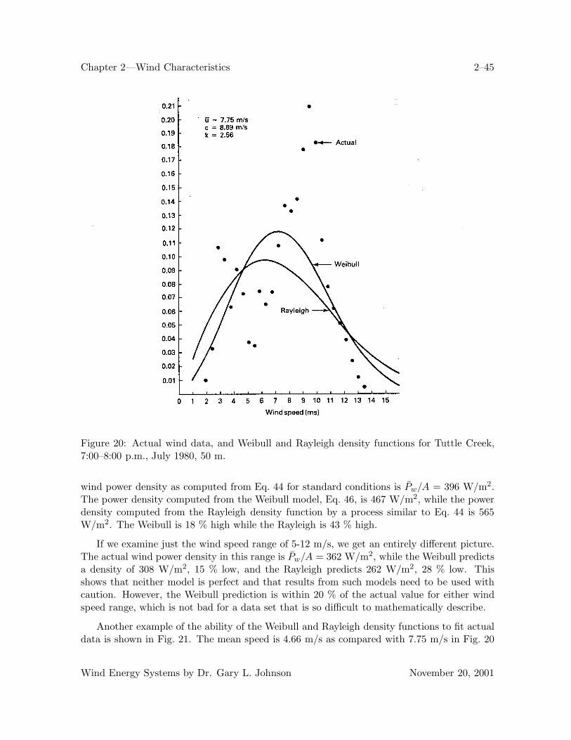
Chapter 2—Wind Characteristics 2–45
Figure 20: Actual wind data, and Weibull and Rayleigh density functions for Tuttle Creek,7:00–8:00 p.m., July 1980, 50 m.
wind power density as computed from Eq. 44 for standard conditions is Pw/A = 396 W/m2.The power density computed from the Weibull model, Eq. 46, is 467 W/m2, while the powerdensity computed from the Rayleigh density function by a process similar to Eq. 44 is 565W/m2. The Weibull is 18 % high while the Rayleigh is 43 % high.
If we examine just the wind speed range of 5-12 m/s, we get an entirely different picture.The actual wind power density in this range is Pw/A = 362 W/m2, while the Weibull predictsa density of 308 W/m2, 15 % low, and the Rayleigh predicts 262 W/m2, 28 % low. Thisshows that neither model is perfect and that results from such models need to be used withcaution. However, the Weibull prediction is within 20 % of the actual value for either windspeed range, which is not bad for a data set that is so difficult to mathematically describe.
Another example of the ability of the Weibull and Rayleigh density functions to fit actualdata is shown in Fig. 21. The mean speed is 4.66 m/s as compared with 7.75 m/s in Fig. 20
Wind Energy Systems by Dr. Gary L. Johnson November 20, 2001
Chapter 2—Wind Characteristics 2–46
and k is 1.61 as compared with 2.56. This decrease in k to a value below 2 causes the Weibulldensity function to be below the Rayleigh function over a central range of wind speeds, in thiscase 2–8 m/s. The actual data are concentrated between 2 and 4 m/s and neither function isable to follow this wide variation. The actual wind power density in this case is 168 W/m2,while the Weibull prediction is 161 W/m2, 4 % low, and the Rayleigh prediction is 124 W/m2,26 % low. Considering only the 5–12 m/s range, the actual power density is 89 W/m2, theWeibull prediction is 133 W/m2, 49 % high, and the Rayleigh prediction is 109 W/m2, 22 %high.
Figure 21: Actual wind data, and Weibull and Rayleigh density functions for Tuttle Creek,7:00–8:00 a.m., August 1980, 10 m.
We see from these two figures that it is difficult to make broad generalizations about theability of the Weibull and Rayleigh density functions to fit actual data. Either one may beeither high or low in a particular range. The final test or proof of the usefulness of thesefunctions will be in their ability to predict the power output of actual wind turbines. In the
Wind Energy Systems by Dr. Gary L. Johnson November 20, 2001
Chapter 2—Wind Characteristics 2–47
meantime it appears that either function may yield acceptable results, with the Weibull beingmore accurate and the Rayleigh easier to use.
Although the actual wind speed distribution can be described by either a Weibull or aRayleigh density function, there are other quantities which are better described by a normaldistribution. The distribution of monthly or yearly mean speeds is likely to be normallydistributed around a long-term mean wind speed, for example. The normal curve is certainlythe best known and most widely used distribution for a continuous random variable, so weshall mention a few of its properties.
The density function f(u) of a normal distribution is
f(u) =1
σ√
2πexp
[−(u − u)2
2σ2
](63)
where u is the mean and σ is the standard deviation. In this expression, the variable u isallowed to vary from −∞ to +∞. It is physically impossible for a wind speed to be negative,of course, so we cannot forget the reality of the observed quantity and follow the mathematicalmodel past this point. This will not usually present any difficulty in examining mean windspeeds.
The cumulative distribution function F (u) is given by
F (u) =∫ u
−∞f(x)dx (64)
This integral does not have a simple closed form solution, so tables of values are determinedfrom approximate integration methods. The variable in this table is usually defined as
q =u − u
σor u = u + qσ (65)
Thus q is the number of standard deviations that u is away from u. A brief version of thistable is shown in Table 2.4. We see from the table, for example, that F (u) for a wind speedone standard deviation below the mean is 0.159. This means there is a 15.9 % probabilitythat the mean speed for any period of interest will be more than one standard deviation belowthe long term mean. Since the normal density function is symmetrical, there is also a 15.9% probability that the mean speed for some period will be more than one standard deviationabove the long term mean.
Wind Energy Systems by Dr. Gary L. Johnson November 20, 2001
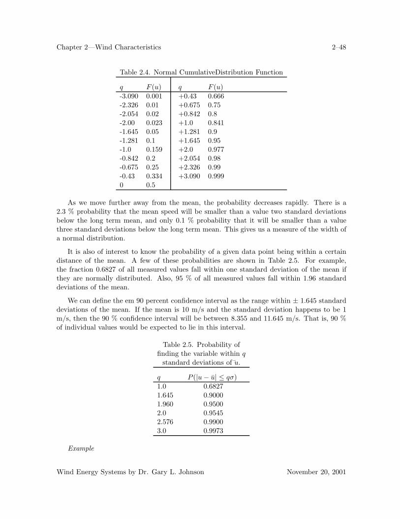
Chapter 2—Wind Characteristics 2–48
Table 2.4. Normal CumulativeDistribution Function
q F (u) q F (u)-3.090 0.001 +0.43 0.666-2.326 0.01 +0.675 0.75-2.054 0.02 +0.842 0.8-2.00 0.023 +1.0 0.841-1.645 0.05 +1.281 0.9-1.281 0.1 +1.645 0.95-1.0 0.159 +2.0 0.977-0.842 0.2 +2.054 0.98-0.675 0.25 +2.326 0.99-0.43 0.334 +3.090 0.9990 0.5
As we move further away from the mean, the probability decreases rapidly. There is a2.3 % probability that the mean speed will be smaller than a value two standard deviationsbelow the long term mean, and only 0.1 % probability that it will be smaller than a valuethree standard deviations below the long term mean. This gives us a measure of the width ofa normal distribution.
It is also of interest to know the probability of a given data point being within a certaindistance of the mean. A few of these probabilities are shown in Table 2.5. For example,the fraction 0.6827 of all measured values fall within one standard deviation of the mean ifthey are normally distributed. Also, 95 % of all measured values fall within 1.96 standarddeviations of the mean.
We can define the em 90 percent confidence interval as the range within ± 1.645 standarddeviations of the mean. If the mean is 10 m/s and the standard deviation happens to be 1m/s, then the 90 % confidence interval will be between 8.355 and 11.645 m/s. That is, 90 %of individual values would be expected to lie in this interval.
Table 2.5. Probability offinding the variable within q
standard deviations of u.
q P (|u − u| ≤ qσ)1.0 0.68271.645 0.90001.960 0.95002.0 0.95452.576 0.99003.0 0.9973
Example
Wind Energy Systems by Dr. Gary L. Johnson November 20, 2001
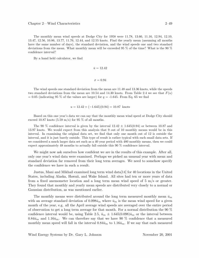
Chapter 2—Wind Characteristics 2–49
The monthly mean wind speeds at Dodge City for 1958 were 11.78, 13.66, 11.16, 12.94, 12.10,13.47, 12.56, 10.86, 13.77, 11.76, 12.44, and 12.55 knots. Find the yearly mean (assuming all monthshave the same number of days), the standard deviation, and the wind speeds one and two standarddeviations from the mean. What monthly mean will be exceeded 95 % of the time? What is the 90 %confidence interval?
By a hand held calculator, we find
u = 12.42
σ = 0.94
The wind speeds one standard deviation from the mean are 11.48 and 13.36 knots, while the speedstwo standard deviations from the mean are 10.54 and 14.30 knots. From Table 2.4 we see that F (u)= 0.05 (indicating 95 % of the values are larger) for q = -1.645. From Eq. 65 we find
u = 12.42 + (−1.645)(0.94) = 10.87 knots
Based on this one year’s data we can say that the monthly mean wind speed at Dodge City shouldexceed 10.87 knots (5.59 m/s) for 95 % of all months.
The 90 % confidence interval is given by the interval 12.42 ± 1.645(0.94) or between 10.87 and13.97 knots. We would expect from this analysis that 9 out of 10 monthly means would be in thisinterval. In examining the original data set, we find that only one month out of 12 is outside theinterval, and it is just barely outside. This type of result is rather typical with such small data sets. Ifwe considered a much larger data set such as a 40 year period with 480 monthly means, then we couldexpect approximately 48 months to actually fall outside this 90 % confidence interval.
We might now ask ourselves how confident we are in the results of this example. After all,only one year’s wind data were examined. Perhaps we picked an unusual year with mean andstandard deviation far removed from their long term averages. We need to somehow specifythe confidence we have in such a result.
Justus, Mani and Mikhail examined long term wind data[14] for 40 locations in the UnitedStates, including Alaska, Hawaii, and Wake Island. All sites had ten or more years of datafrom a fixed anemometer location and a long term mean wind speed of 5 m/s or greater.They found that monthly and yearly mean speeds are distributed very closely to a normal orGaussian distribution, as was mentioned earlier.
The monthly means were distributed around the long term measured monthly mean um
with an average standard deviation of 0.098um where um is the mean wind speed for a givenmonth of the year, e.g. all the April average wind speeds are averaged over the entire periodof observation to get a long term average for that month. For a normal distribution the 90 %confidence interval would be, using Table 2.5, um ± 1.645(0.098)um or the interval between0.84um and 1.16um. We can therefore say that we have 90 % confidence that a measuredmonthly mean speed will fall in the interval 0.84um to 1.16um. If we say that each measured
Wind Energy Systems by Dr. Gary L. Johnson November 20, 2001
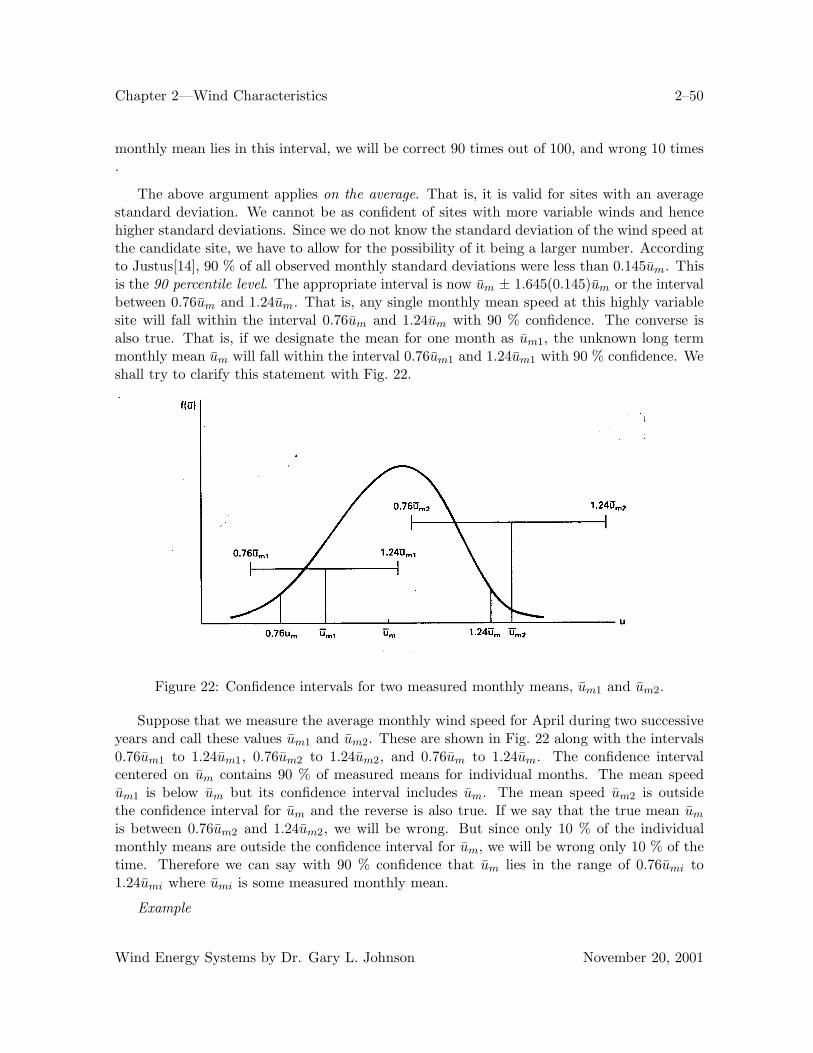
Chapter 2—Wind Characteristics 2–50
monthly mean lies in this interval, we will be correct 90 times out of 100, and wrong 10 times.
The above argument applies on the average. That is, it is valid for sites with an averagestandard deviation. We cannot be as confident of sites with more variable winds and hencehigher standard deviations. Since we do not know the standard deviation of the wind speed atthe candidate site, we have to allow for the possibility of it being a larger number. Accordingto Justus[14], 90 % of all observed monthly standard deviations were less than 0.145um. Thisis the 90 percentile level. The appropriate interval is now um ± 1.645(0.145)um or the intervalbetween 0.76um and 1.24um. That is, any single monthly mean speed at this highly variablesite will fall within the interval 0.76um and 1.24um with 90 % confidence. The converse isalso true. That is, if we designate the mean for one month as um1, the unknown long termmonthly mean um will fall within the interval 0.76um1 and 1.24um1 with 90 % confidence. Weshall try to clarify this statement with Fig. 22.
Figure 22: Confidence intervals for two measured monthly means, um1 and um2.
Suppose that we measure the average monthly wind speed for April during two successiveyears and call these values um1 and um2. These are shown in Fig. 22 along with the intervals0.76um1 to 1.24um1, 0.76um2 to 1.24um2, and 0.76um to 1.24um. The confidence intervalcentered on um contains 90 % of measured means for individual months. The mean speedum1 is below um but its confidence interval includes um. The mean speed um2 is outsidethe confidence interval for um and the reverse is also true. If we say that the true mean um
is between 0.76um2 and 1.24um2, we will be wrong. But since only 10 % of the individualmonthly means are outside the confidence interval for um, we will be wrong only 10 % of thetime. Therefore we can say with 90 % confidence that um lies in the range of 0.76umi to1.24umi where umi is some measured monthly mean.
Example
Wind Energy Systems by Dr. Gary L. Johnson November 20, 2001
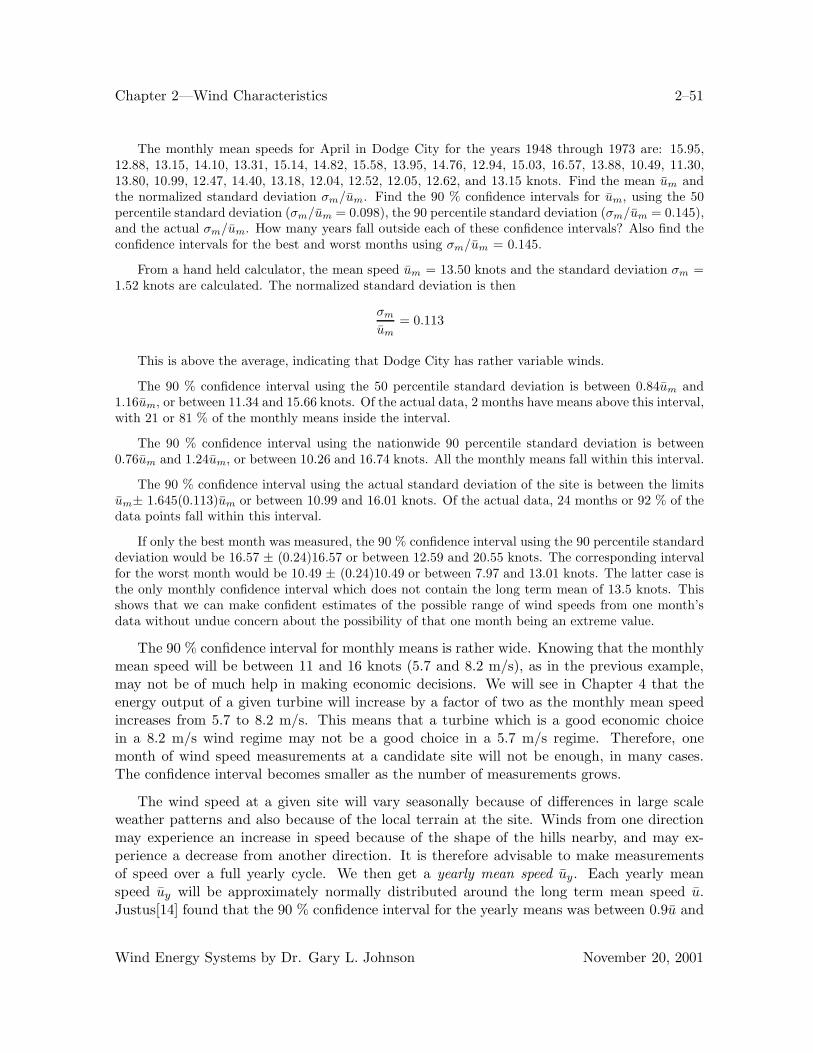
Chapter 2—Wind Characteristics 2–51
The monthly mean speeds for April in Dodge City for the years 1948 through 1973 are: 15.95,12.88, 13.15, 14.10, 13.31, 15.14, 14.82, 15.58, 13.95, 14.76, 12.94, 15.03, 16.57, 13.88, 10.49, 11.30,13.80, 10.99, 12.47, 14.40, 13.18, 12.04, 12.52, 12.05, 12.62, and 13.15 knots. Find the mean um andthe normalized standard deviation σm/um. Find the 90 % confidence intervals for um, using the 50percentile standard deviation (σm/um = 0.098), the 90 percentile standard deviation (σm/um = 0.145),and the actual σm/um. How many years fall outside each of these confidence intervals? Also find theconfidence intervals for the best and worst months using σm/um = 0.145.
From a hand held calculator, the mean speed um = 13.50 knots and the standard deviation σm =1.52 knots are calculated. The normalized standard deviation is then
σm
um= 0.113
This is above the average, indicating that Dodge City has rather variable winds.
The 90 % confidence interval using the 50 percentile standard deviation is between 0.84um and1.16um, or between 11.34 and 15.66 knots. Of the actual data, 2 months have means above this interval,with 21 or 81 % of the monthly means inside the interval.
The 90 % confidence interval using the nationwide 90 percentile standard deviation is between0.76um and 1.24um, or between 10.26 and 16.74 knots. All the monthly means fall within this interval.
The 90 % confidence interval using the actual standard deviation of the site is between the limitsum± 1.645(0.113)um or between 10.99 and 16.01 knots. Of the actual data, 24 months or 92 % of thedata points fall within this interval.
If only the best month was measured, the 90 % confidence interval using the 90 percentile standarddeviation would be 16.57 ± (0.24)16.57 or between 12.59 and 20.55 knots. The corresponding intervalfor the worst month would be 10.49 ± (0.24)10.49 or between 7.97 and 13.01 knots. The latter case isthe only monthly confidence interval which does not contain the long term mean of 13.5 knots. Thisshows that we can make confident estimates of the possible range of wind speeds from one month’sdata without undue concern about the possibility of that one month being an extreme value.
The 90 % confidence interval for monthly means is rather wide. Knowing that the monthlymean speed will be between 11 and 16 knots (5.7 and 8.2 m/s), as in the previous example,may not be of much help in making economic decisions. We will see in Chapter 4 that theenergy output of a given turbine will increase by a factor of two as the monthly mean speedincreases from 5.7 to 8.2 m/s. This means that a turbine which is a good economic choicein a 8.2 m/s wind regime may not be a good choice in a 5.7 m/s regime. Therefore, onemonth of wind speed measurements at a candidate site will not be enough, in many cases.The confidence interval becomes smaller as the number of measurements grows.
The wind speed at a given site will vary seasonally because of differences in large scaleweather patterns and also because of the local terrain at the site. Winds from one directionmay experience an increase in speed because of the shape of the hills nearby, and may ex-perience a decrease from another direction. It is therefore advisable to make measurementsof speed over a full yearly cycle. We then get a yearly mean speed uy. Each yearly meanspeed uy will be approximately normally distributed around the long term mean speed u.Justus[14] found that the 90 % confidence interval for the yearly means was between 0.9u and
Wind Energy Systems by Dr. Gary L. Johnson November 20, 2001
Chapter 2—Wind Characteristics 2–52
1.1u for the median (50 percentile) standard deviation and between 0.85u and 1.15u for the90 percentile standard deviation. As expected, these are narrower confidence intervals thanwere observed for the single monthly mean.
Example
The yearly mean speed at Dodge City was 11.44 knots at 7 m above the ground level in 1973.Assume a 50 percentile standard deviation and determine the 90 % confidence interval for the truelong term mean speed.
The confidence interval extends from 11.44/1.1 = 10.40 to 11.44/0.9 = 12.71 knots. We cantherefore say that the long term mean speed lies between 10.40 and 12.71 knots with 90 % confidence.
Our estimate of the long term mean speed by one year’s data can conceivably be improvedby comparing our one year mean speed to that of a nearby National Weather Service station.If the yearly mean speed at the NWS station was higher than the long term mean speed there,the measured mean speed at the candidate site can be adjusted upward by the same factor.This assumes that all the winds within a geographical region of similar topography and adiameter up to a few hundred kilometers will have similar year to year variations. If the longterm mean speed at the NWS station is u, the mean for one year is ua, and the mean for thesame year at the candidate site is ub, then the corrected or estimated long term mean speeduc at the candidate site is
uc = ubu
ua(66)
Note that we do not know how to assign a confidence interval to this estimate. It is a singlenumber whose accuracy depends on both the accuracy of u and the correlation between ua andub. The accuracy of u should be reasonably good after 30 or more years of measurements, asis common in many NWS stations. However, the assumed correlation between ua and ub maynot be very good. Justus[14] found that the correlation was poor enough that the estimate oflong term means was not improved by using data from nearby stations. Equally good resultswould be obtained by applying the 90 % confidence interval approach as compared to usingEq. 66. The reason for this phenomenon was not determined. One possibility is that the typeof anemometer used by the National Weather Service can easily get dirty and yield resultsthat are low by 10 to 20 % until the next maintenance period. One NWS station may have afew months of low readings one year while another NWS station may have a few months oflow readings the next year, due to the measuring equipment rather than the wind. This wouldmake a correction like Eq. 66 very difficult to use. If this is the problem, it can be reducedby using an average of several NWS stations and, of course, by more frequent maintenance.Other studies are necessary to clarify this situation.
The actual correlation between two sites can be defined in terms of a correlation coefficientr, where
Wind Energy Systems by Dr. Gary L. Johnson November 20, 2001
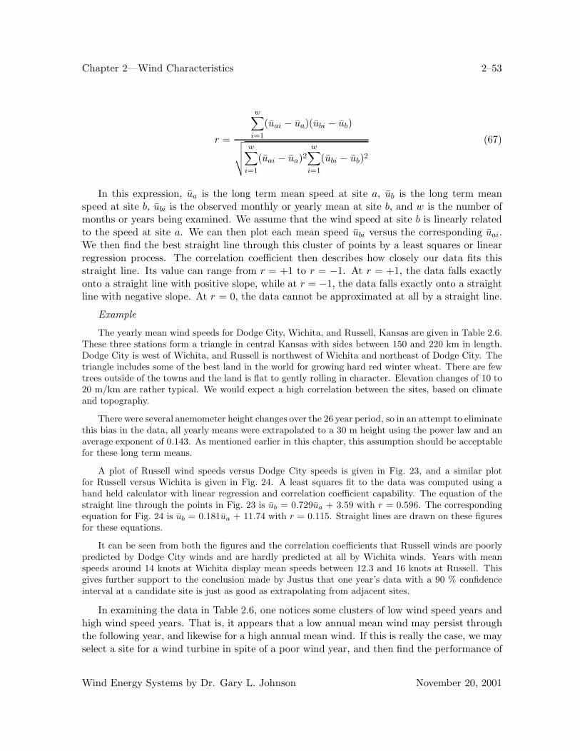
Chapter 2—Wind Characteristics 2–53
r =
w∑i=1
(uai − ua)(ubi − ub)
√√√√ w∑i=1
(uai − ua)2w∑
i=1
(ubi − ub)2(67)
In this expression, ua is the long term mean speed at site a, ub is the long term meanspeed at site b, ubi is the observed monthly or yearly mean at site b, and w is the number ofmonths or years being examined. We assume that the wind speed at site b is linearly relatedto the speed at site a. We can then plot each mean speed ubi versus the corresponding uai.We then find the best straight line through this cluster of points by a least squares or linearregression process. The correlation coefficient then describes how closely our data fits thisstraight line. Its value can range from r = +1 to r = −1. At r = +1, the data falls exactlyonto a straight line with positive slope, while at r = −1, the data falls exactly onto a straightline with negative slope. At r = 0, the data cannot be approximated at all by a straight line.
Example
The yearly mean wind speeds for Dodge City, Wichita, and Russell, Kansas are given in Table 2.6.These three stations form a triangle in central Kansas with sides between 150 and 220 km in length.Dodge City is west of Wichita, and Russell is northwest of Wichita and northeast of Dodge City. Thetriangle includes some of the best land in the world for growing hard red winter wheat. There are fewtrees outside of the towns and the land is flat to gently rolling in character. Elevation changes of 10 to20 m/km are rather typical. We would expect a high correlation between the sites, based on climateand topography.
There were several anemometer height changes over the 26 year period, so in an attempt to eliminatethis bias in the data, all yearly means were extrapolated to a 30 m height using the power law and anaverage exponent of 0.143. As mentioned earlier in this chapter, this assumption should be acceptablefor these long term means.
A plot of Russell wind speeds versus Dodge City speeds is given in Fig. 23, and a similar plotfor Russell versus Wichita is given in Fig. 24. A least squares fit to the data was computed using ahand held calculator with linear regression and correlation coefficient capability. The equation of thestraight line through the points in Fig. 23 is ub = 0.729ua + 3.59 with r = 0.596. The correspondingequation for Fig. 24 is ub = 0.181ua + 11.74 with r = 0.115. Straight lines are drawn on these figuresfor these equations.
It can be seen from both the figures and the correlation coefficients that Russell winds are poorlypredicted by Dodge City winds and are hardly predicted at all by Wichita winds. Years with meanspeeds around 14 knots at Wichita display mean speeds between 12.3 and 16 knots at Russell. Thisgives further support to the conclusion made by Justus that one year’s data with a 90 % confidenceinterval at a candidate site is just as good as extrapolating from adjacent sites.
In examining the data in Table 2.6, one notices some clusters of low wind speed years andhigh wind speed years. That is, it appears that a low annual mean wind may persist throughthe following year, and likewise for a high annual mean wind. If this is really the case, we mayselect a site for a wind turbine in spite of a poor wind year, and then find the performance of
Wind Energy Systems by Dr. Gary L. Johnson November 20, 2001

Chapter 2—Wind Characteristics 2–54
Table 2.6 Average yearly speeds corrected to 30 m (100 ft)Year Dodge City Wichita Russell1948 14.98 14.09 14.14a
1949 13.53 13.35 13.08b
1950 12.89 12.77 14.111951 13.83 13.47 13.071952 14.22 13.97 12.311953 15.57 14.45c 13.371954 15.20 14.98 12.831955 14.83 15.22 14.891956 14.60 14.86 14.851957 14.71 13.60 15.381958 13.85 13.74 13.631959 14.91 15.21 14.881960 15.23 14.55 13.671961 12.37 13.29 12.451962 13.53 13.18 12.991963 14.90 12.74 15.201964 16.32 13.95 16.041965 15.17 13.46 14.711966 15.37 13.40 15.171967 15.26 13.78 15.201968 15.25 14.51 15.70d
1969 14.19 13.33 14.52e
1970 14.85 14.11 15.661971 15.04 13.97 15.011972 14.40 13.84 13.391973 15.35 13.87 14.41
aEstimated from 50, 51, 52 data by method of ratios.bEstimated from 50, 51, 52 data by method of ratios.cEstimated from 50, 51, 52 data by method of ratios.dEstimated from 66, 67, 70, 71 data by method of ratios.eEstimated from 66, 67, 70, 71 data by method of ratios.
the wind turbine to be poor in the first year after installation. This has economic implicationsbecause the cash flow requirements will usually be most critical the first year after installation.The turbine may go ahead and deliver the expected amount of energy over its lifetime, butthis does not help the economic situation immediately after installation. Justus[14] examinedthis question also, for 40 sites in the United States, and concluded that there is about a 60% probability that one low wind speed month or year will be followed by a similar one. Ifwind speeds were totally random, then this probability would be 50 %, the same as for twoheads in a row when flipping a coin. The probability of an additional low speed month or
Wind Energy Systems by Dr. Gary L. Johnson November 20, 2001

Chapter 2—Wind Characteristics 2–55
Figure 23: Yearly mean wind speeds (knots) at Russell, Kansas, versus simultaneous speedsat Dodge City, Kansas.
year following the first two is totally random. Based on these results, Justus concluded thatclusters of bad wind months or years are not highly probable. In fact, the variation of speedfrom one period to the next is almost totally random, and therefore such clusters should notbe of major concern.
We have seen that the 90 % confidence interval for the long term annual mean speed at asite is between 0.9u and 1.1u when only one year’s data is collected. If this is not adequate,then additional data need to be collected. Corotis[7] reports that the 90 % confidence intervalis between 0.93u and 1.07u for two year’s data, and between 0.94u and 1.06u for three year’sdata. The confidence interval is basically inversely proportional to the square root of the timeperiod, so additional years of data reduce the confidence interval at a slower and slower rate.
10 DISTRIBUTION OF EXTREME WINDS
Two important wind speeds which affect turbine cost are the design wind speed which therotor can withstand in a parked rotor configuration, and the maximum operating wind speed.A typical wind turbine may start producing power at 5 to 7 m/s (11 to 16 mi/h), reach ratedpower at 12 to 16 m/s (27 to 36 mi/h), and be shut down at a maximum operating speed of20 to 25 m/s (45 to 56 mi/h).
Wind Energy Systems by Dr. Gary L. Johnson November 20, 2001
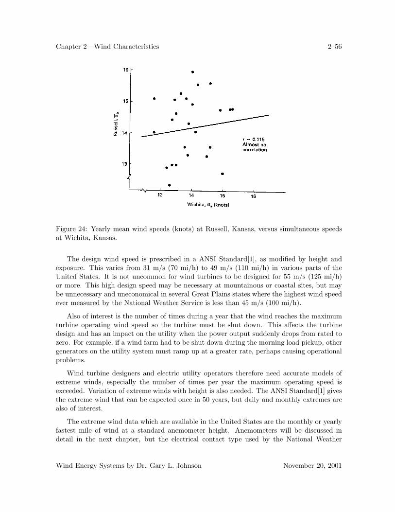
Chapter 2—Wind Characteristics 2–56
Figure 24: Yearly mean wind speeds (knots) at Russell, Kansas, versus simultaneous speedsat Wichita, Kansas.
The design wind speed is prescribed in a ANSI Standard[1], as modified by height andexposure. This varies from 31 m/s (70 mi/h) to 49 m/s (110 mi/h) in various parts of theUnited States. It is not uncommon for wind turbines to be designed for 55 m/s (125 mi/h)or more. This high design speed may be necessary at mountainous or coastal sites, but maybe unnecessary and uneconomical in several Great Plains states where the highest wind speedever measured by the National Weather Service is less than 45 m/s (100 mi/h).
Also of interest is the number of times during a year that the wind reaches the maximumturbine operating wind speed so the turbine must be shut down. This affects the turbinedesign and has an impact on the utility when the power output suddenly drops from rated tozero. For example, if a wind farm had to be shut down during the morning load pickup, othergenerators on the utility system must ramp up at a greater rate, perhaps causing operationalproblems.
Wind turbine designers and electric utility operators therefore need accurate models ofextreme winds, especially the number of times per year the maximum operating speed isexceeded. Variation of extreme winds with height is also needed. The ANSI Standard[1] givesthe extreme wind that can be expected once in 50 years, but daily and monthly extremes arealso of interest.
The extreme wind data which are available in the United States are the monthly or yearlyfastest mile of wind at a standard anemometer height. Anemometers will be discussed indetail in the next chapter, but the electrical contact type used by the National Weather
Wind Energy Systems by Dr. Gary L. Johnson November 20, 2001
Chapter 2—Wind Characteristics 2–57
Service stations will be mentioned briefly here. Its three-cup rotor drives a gear train whichmomentarily closes a switch after a fixed number of revolutions. The cup speed is proportionalto the wind speed so contact is made with the passage of a fixed amount of air by or throughthe anemometer. The anemometer can be calibrated so the switch makes contact once withevery mile of wind that passes it. If the wind is blowing at 60 mi/h, then a mile of wind willpass the anemometer in one minute.
The contact anemometer is obviously an averaging device. It gives the average speed ofthe fastest mile, which will be smaller than the average speed of the fastest 1/10th mile, orany other fraction of a mile, because of the fluctuation of wind speed with time. But one hasto stop refining data at some point, and the fastest mile seems to have been that point forstructural studies.
The procedure is to fit a probability distribution function to the observed high wind speeddata. The Weibull distribution function of Eq. 30 could probably be used for this function,except that it tends to zero somewhat too fast. It is convenient to define a new distributionfunction Fe(u) just for the extreme winds.
Weather related extreme events, such as floods or extreme winds[11], are usually describedin terms of one of two Fisher-Tippett distributions, the Type I or Type II. Thom[23, 24] usedthe Type II to describe extreme winds in the United States. He prepared a series of mapsbased on annual extremes, showing the fastest mile for recurrence intervals of 2, 50, and100 years. Height corrections were made by applying the one-seventh power law. NationalWeather Service data were used.
The ANSI Standard[1] is based on examination of a longer period of record by Simiu[21]and uses the Type I distribution. Only a single map is given, for a recurrence interval of 50years. Other recurrence intervals are obtained from this map by a multiplying factor. Tablesare given for the variation of wind speed with height.
Careful study of a large data set collected by Johnson and analyzed by Henry[12] showedthat the Type I distribution is superior to the Type II, so the mathematical description foronly the Type I will be discussed here. The Fisher-Tippett Type I distribution has the form
Fe(u) = exp(− exp(−α(x − β))) (68)
where Fe(u) is the probability of the annual fastest mile of wind speed being less than u. Theparameters α and β are characteristics of the site that must be estimated from the observeddata. If n period extremes are available, the maximum likelihood estimate of α may beobtained by choosing an initial guess and iterating
Wind Energy Systems by Dr. Gary L. Johnson November 20, 2001
Chapter 2—Wind Characteristics 2–58
αi+1 =1
x −
n∑j=1
xj exp(−αixj)
n∑j=1
exp(−αixj)
(69)
until convergence to some value α. The maximum likelihood estimate of β is
β = x − 0.5772α
(70)
If Fe(u) = 0.5, then u is the median annual fastest mile. Half the years will have a fasterannual extreme mile and half the years will have a slower one. Statistically, the average timeof recurrence of speeds greater than this median value will be two years. Similar argumentscan be made to develop a general relationship for the mean recurrence interval Mr, which is
Mr =1
1 − Fe(u)(71)
which yields
u = − 1α
ln(− ln(1 − 1
Mr
)+ β (72)
A mean recurrence interval of 50 years would require Fe(u) = 0.98, for example.
Example
At a given location, the parameters of Eq. 68 are determined to be γ = 4 and β = 20 m/s. Whatis the mean recurrence interval of a 40 m/s extreme wind speed?
From Eq. 68 we find that
Fe(40) = exp
[−(
4020
)−4]
= 0.939
From Eq. 67, the mean recurrence interval is
Mr =1
1 − 0.939= 16.4
At this location, a windspeed of 40 m/s would be expected about once every 16 years, on theaverage.
If we have 20 years or more of data, then it is most appropriate to find the distributionof yearly extremes. We use one value for each year and calculate α and β. If we have only
Wind Energy Systems by Dr. Gary L. Johnson November 20, 2001
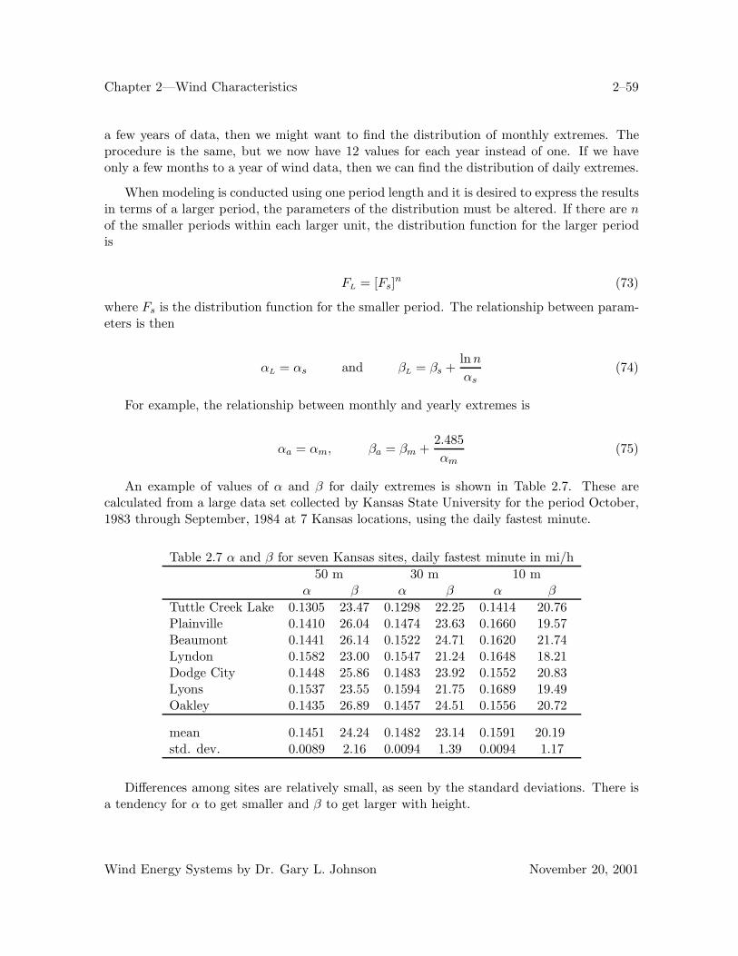
Chapter 2—Wind Characteristics 2–59
a few years of data, then we might want to find the distribution of monthly extremes. Theprocedure is the same, but we now have 12 values for each year instead of one. If we haveonly a few months to a year of wind data, then we can find the distribution of daily extremes.
When modeling is conducted using one period length and it is desired to express the resultsin terms of a larger period, the parameters of the distribution must be altered. If there are nof the smaller periods within each larger unit, the distribution function for the larger periodis
FL = [Fs]n (73)
where Fs is the distribution function for the smaller period. The relationship between param-eters is then
αL = αs and βL = βs +ln n
αs(74)
For example, the relationship between monthly and yearly extremes is
αa = αm, βa = βm +2.485αm
(75)
An example of values of α and β for daily extremes is shown in Table 2.7. These arecalculated from a large data set collected by Kansas State University for the period October,1983 through September, 1984 at 7 Kansas locations, using the daily fastest minute.
Table 2.7 α and β for seven Kansas sites, daily fastest minute in mi/h50 m 30 m 10 m
α β α β α β
Tuttle Creek Lake 0.1305 23.47 0.1298 22.25 0.1414 20.76Plainville 0.1410 26.04 0.1474 23.63 0.1660 19.57Beaumont 0.1441 26.14 0.1522 24.71 0.1620 21.74Lyndon 0.1582 23.00 0.1547 21.24 0.1648 18.21Dodge City 0.1448 25.86 0.1483 23.92 0.1552 20.83Lyons 0.1537 23.55 0.1594 21.75 0.1689 19.49Oakley 0.1435 26.89 0.1457 24.51 0.1556 20.72
mean 0.1451 24.24 0.1482 23.14 0.1591 20.19std. dev. 0.0089 2.16 0.0094 1.39 0.0094 1.17
Differences among sites are relatively small, as seen by the standard deviations. There isa tendency for α to get smaller and β to get larger with height.
Wind Energy Systems by Dr. Gary L. Johnson November 20, 2001

Chapter 2—Wind Characteristics 2–60
Similar data for 5 Kansas National Weather Service Stations for the same time period isshown in Table 2.8. The fastest mile is used rather than the fastest minute, which theoreticallymakes only a small difference.
Table 2.8 α and β for five Kansas NWS Stations, daily fastest mile.
α β Height in ftWichita 0.2051 17.01 25Topeka 0.2068 14.89 20Concordia 0.2149 17.45 33Goodland 0.2272 18.20 20Dodge City 0.2060 19.46 20
mean 0.2120 17.40std. dev. 0.0094 1.68
Differences among the NWS sites are also relatively small. However, the NWS sites havea consistently larger α and smaller β than the KSU sites in Table 2.7. Both differencescause the predicted extreme wind to be smaller at the NWS sites than at the KSU sites.In making a detailed comparison of the Dodge City NWS and the Dodge City KSU sites,which are about 5 miles apart in similar terrain, it appears that the difference was causedby the type of anemometer used. The KSU study used the Maximum anemometer, a small,light, and inexpensive device, while the National Weather Service used the Electric SpeedIndicator anemometer, a much larger and heavier device. The 10 m mean speed with theKSU equipment was 12.8 mi/h for the year, while the NWS mean was 14.1 mi/h, so theMaximum anemometer indicated a mean speed 9 % below the NWS mean. On the otherhand, the extreme winds measured by the Maximum anemometer averaged 18 % higher thanthe NWS extremes. The Maximum anemometer indication for the extreme winds varied fromabout the same as the NWS measurement to as much as 15 mi/h faster. It is evident that thetype of measurement equipment can make a significant difference in the results.
A longer period of time was then analyzed for two of the NWS Stations, using monthlyextremes rather than daily extremes. The results of this study are shown in Table 2.9.
Table 2.9. α and β for Topeka and Dodge City,using monthly fastest mile for 1949–1968.
α β
Topeka 0.1420 34.38Dodge City 0.1397 41.94
The fastest mile observed at Dodge City for this period was 77 mi/h, while at Topekait was 74 mi/h. The α values are much closer to the KSU values than to the NWS valuesfor the one year study. The β values are larger as required by Eq. 74. From these values
Wind Energy Systems by Dr. Gary L. Johnson November 20, 2001

Chapter 2—Wind Characteristics 2–61
for Dodge City, the extreme wind expected once every 3.3 months (approximately 100 days)would be 49.23 mi/h, a value surprisingly close to the prediction using the KSU data anddaily extremes.
As mentioned earlier, it is important to have an estimate of the number of days during ayear in which the wind speed should equal or exceed a given value. This is done by insertingvalues of α, β, and the given wind speed in Eq. 68, then using Eq. 69 to find Mr, and finallytaking the reciprocal of the interval Mr to find the frequency. Values are given in Table 2.10for the mean KSU parameters, the mean NWS parameters from Table 2.8, and the meanNWS parameters for monthly extremes from Table 2.9, all expressed in days per year for awind speed in mi/h.
Table 2.10. Days per year a givenwind speed or greater is observed.
speed 50 m 30 m 10 m NWS Topeka DodgeCity
30 128.4 110.8 69.1 39.335 69.1 57.8 33.0 14.640 35.3 28.8 15.3 5.3 4.4 8.845 17.5 14.0 7.0 1.9 2.4 5.850 8.6 6.8 3.2 0.7 1.2 3.355 4.2 3.2 1.4 0.2 0.6 1.860 2.0 1.6 0.6 0.1 0.3 0.9
There is some scatter in the results, as has been previously discussed, but the resultsare still quite acceptable for many purposes. For example, a wind turbine with a maximumoperating speed of 45 mi/h and a height of 10 m or less would be expected to be shut downbetween 2 and 7 times per year. If the turbine height were increased to 30 m, the numberof shutdowns would approximately double, from 7 to 14. Increasing the maximum operatingspeed by 5 mi/h will cut the number of shutdowns in half. These rules of thumb may be quiteuseful to system designers.
As mentioned earlier, Thom[23] has analyzed 141 open-country stations averaging about15 years of data per station and has published results for Fe(u) = 0.5, 0.98, and 0.99 whichcorrespond to mean times between occurrences of 2, 50, and 100 years, respectively. Thesecurves are given in Figs. 25–27. Since he used the Type II distribution, the absolute valuesare not as accurate as we get from the Type I. However, the trends are the same with eitherdistribution and illustrate some very interesting facts about the geographical variation ofextreme winds.
The curve for the 2 year mean recurrence interval gives results which might be anticipatedfrom information on average winds presented earlier in the chapter. The High Plains have thehighest extreme wind speeds and the southeastern and southwestern United States have thelowest. This relationship is basically the same as that for the average wind speeds. The 50
Wind Energy Systems by Dr. Gary L. Johnson November 20, 2001
Chapter 2—Wind Characteristics 2–62
year and 100 year curves are distinctly different, however. The once a century extreme windin Western Kansas, Oklahoma, and Texas is about 40 m/s, a figure exceeded in large areas ofthe coastal regions. The Gulf Coast and Atlantic Coast, as far north as Southern Maine, haveexperienced extreme winds from tropical cyclones, or hurricanes. The effect of these stormsoften extends inland from 100 to 200 miles. The remainder of the United States experiencesextreme winds largely from thunderstorms. This type of storm accounts for over one third ofthe extreme-wind situations in the contiguous United States.
Water areas have a marked effect on extreme wind speeds. Where a location has unob-structed access to a large body of water, extreme winds may be 15 m/s or more greater thana short distance inland. High winds in cyclones and near water tend to remain steady overlonger periods than for thunderstorms. They also tend to be much more widespread in a givensituation and hence cause widespread damage, although damage to individual structures maynot be greater than from thunderstorm winds.
The speed of the greatest gust experienced by a wind turbine will be somewhat greaterthan the speed of the fastest mile because of the averaging which occurs during the periodof measurement. This will vary with the period chosen for the gust measurement and on thespeed of the fastest mile. It appears that a good estimate of a three second gust speed is 1.25times the speed of the fastest mile[15]. That is, if the fastest mile is measured at 40 m/s, thefastest gust will probably be about 1.25(40) = 50 m/s. This is the speed which should beused in talking about survivability of wind turbines.
Standard civil engineering practice calls for ordinary buildings to be designed for a 50year recurrence interval, and for structures whose collapse do not threaten human safety tobe designed for a 25 year recurrence interval. The civil engineers then typically add safetyfactors to their designs which cause the structures to actually withstand higher winds. Asimilar approach would seem appropriate for wind turbines[15]. A 50 year recurrence intervalwould imply that a design for a maximum gust speed of 50 m/s would be adequate overmost of the United States, with perhaps 65 m/s being desirable in hurricane prone areas.Wind turbine costs tend to increase rapidly as the design speed is increased, so rather carefulcost studies are required to insure that the turbine is not over designed. Wind turbines aredifferent from public buildings and bridges in that they would normally fail in high windswithout people getting hurt. It may be less expensive to replace an occasional wind turbinewith a design speed of 50 m/s than to build all wind turbines to withstand 65 m/s.
11 PROBLEMS
1. What is the density of dry air in kg/m3 at standard pressure (101.3 kPa) and
(a) T = 35oC
(b) T = -25oC?
Wind Energy Systems by Dr. Gary L. Johnson November 20, 2001
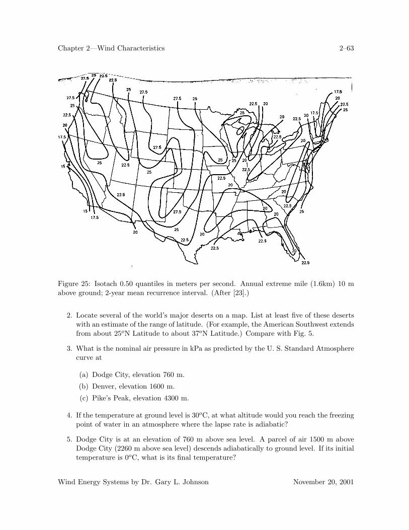
Chapter 2—Wind Characteristics 2–63
Figure 25: Isotach 0.50 quantiles in meters per second. Annual extreme mile (1.6km) 10 mabove ground; 2-year mean recurrence interval. (After [23].)
2. Locate several of the world’s major deserts on a map. List at least five of these desertswith an estimate of the range of latitude. (For example, the American Southwest extendsfrom about 25oN Latitude to about 37oN Latitude.) Compare with Fig. 5.
3. What is the nominal air pressure in kPa as predicted by the U. S. Standard Atmospherecurve at
(a) Dodge City, elevation 760 m.
(b) Denver, elevation 1600 m.
(c) Pike’s Peak, elevation 4300 m.
4. If the temperature at ground level is 30oC, at what altitude would you reach the freezingpoint of water in an atmosphere where the lapse rate is adiabatic?
5. Dodge City is at an elevation of 760 m above sea level. A parcel of air 1500 m aboveDodge City (2260 m above sea level) descends adiabatically to ground level. If its initialtemperature is 0oC, what is its final temperature?
Wind Energy Systems by Dr. Gary L. Johnson November 20, 2001
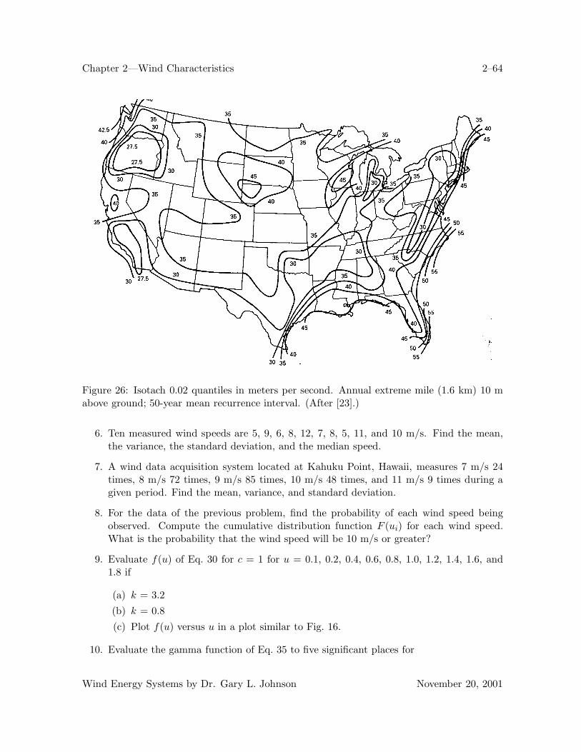
Chapter 2—Wind Characteristics 2–64
Figure 26: Isotach 0.02 quantiles in meters per second. Annual extreme mile (1.6 km) 10 mabove ground; 50-year mean recurrence interval. (After [23].)
6. Ten measured wind speeds are 5, 9, 6, 8, 12, 7, 8, 5, 11, and 10 m/s. Find the mean,the variance, the standard deviation, and the median speed.
7. A wind data acquisition system located at Kahuku Point, Hawaii, measures 7 m/s 24times, 8 m/s 72 times, 9 m/s 85 times, 10 m/s 48 times, and 11 m/s 9 times during agiven period. Find the mean, variance, and standard deviation.
8. For the data of the previous problem, find the probability of each wind speed beingobserved. Compute the cumulative distribution function F (ui) for each wind speed.What is the probability that the wind speed will be 10 m/s or greater?
9. Evaluate f(u) of Eq. 30 for c = 1 for u = 0.1, 0.2, 0.4, 0.6, 0.8, 1.0, 1.2, 1.4, 1.6, and1.8 if
(a) k = 3.2
(b) k = 0.8
(c) Plot f(u) versus u in a plot similar to Fig. 16.
10. Evaluate the gamma function of Eq. 35 to five significant places for
Wind Energy Systems by Dr. Gary L. Johnson November 20, 2001
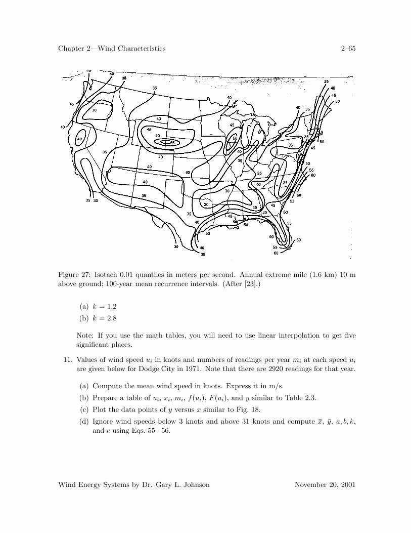
Chapter 2—Wind Characteristics 2–65
Figure 27: Isotach 0.01 quantiles in meters per second. Annual extreme mile (1.6 km) 10 mabove ground; 100-year mean recurrence intervals. (After [23].)
(a) k = 1.2
(b) k = 2.8
Note: If you use the math tables, you will need to use linear interpolation to get fivesignificant places.
11. Values of wind speed ui in knots and numbers of readings per year mi at each speed ui
are given below for Dodge City in 1971. Note that there are 2920 readings for that year.
(a) Compute the mean wind speed in knots. Express it in m/s.
(b) Prepare a table of ui, xi, mi, f(ui), F (ui), and y similar to Table 2.3.
(c) Plot the data points of y versus x similar to Fig. 18.
(d) Ignore wind speeds below 3 knots and above 31 knots and compute x, y, a, b, k,and c using Eqs. 55– 56.
Wind Energy Systems by Dr. Gary L. Johnson November 20, 2001
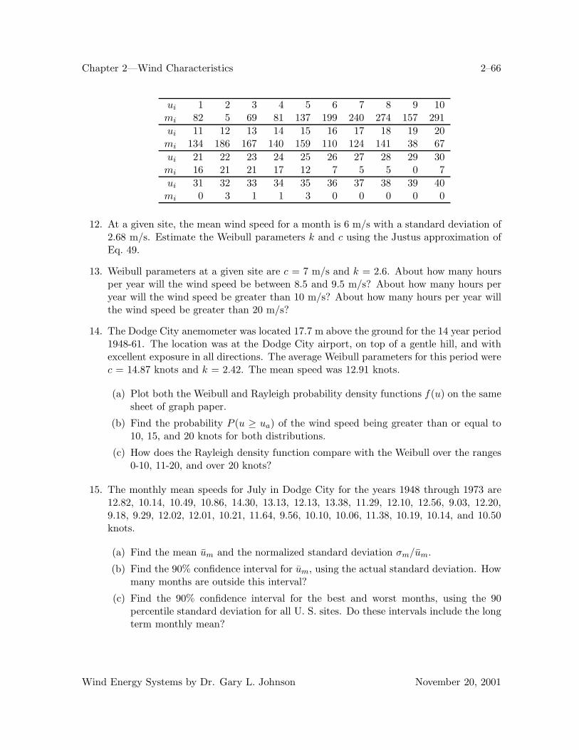
Chapter 2—Wind Characteristics 2–66
ui 1 2 3 4 5 6 7 8 9 10mi 82 5 69 81 137 199 240 274 157 291ui 11 12 13 14 15 16 17 18 19 20mi 134 186 167 140 159 110 124 141 38 67ui 21 22 23 24 25 26 27 28 29 30mi 16 21 21 17 12 7 5 5 0 7ui 31 32 33 34 35 36 37 38 39 40mi 0 3 1 1 3 0 0 0 0 0
12. At a given site, the mean wind speed for a month is 6 m/s with a standard deviation of2.68 m/s. Estimate the Weibull parameters k and c using the Justus approximation ofEq. 49.
13. Weibull parameters at a given site are c = 7 m/s and k = 2.6. About how many hoursper year will the wind speed be between 8.5 and 9.5 m/s? About how many hours peryear will the wind speed be greater than 10 m/s? About how many hours per year willthe wind speed be greater than 20 m/s?
14. The Dodge City anemometer was located 17.7 m above the ground for the 14 year period1948-61. The location was at the Dodge City airport, on top of a gentle hill, and withexcellent exposure in all directions. The average Weibull parameters for this period werec = 14.87 knots and k = 2.42. The mean speed was 12.91 knots.
(a) Plot both the Weibull and Rayleigh probability density functions f(u) on the samesheet of graph paper.
(b) Find the probability P (u ≥ ua) of the wind speed being greater than or equal to10, 15, and 20 knots for both distributions.
(c) How does the Rayleigh density function compare with the Weibull over the ranges0-10, 11-20, and over 20 knots?
15. The monthly mean speeds for July in Dodge City for the years 1948 through 1973 are12.82, 10.14, 10.49, 10.86, 14.30, 13.13, 12.13, 13.38, 11.29, 12.10, 12.56, 9.03, 12.20,9.18, 9.29, 12.02, 12.01, 10.21, 11.64, 9.56, 10.10, 10.06, 11.38, 10.19, 10.14, and 10.50knots.
(a) Find the mean um and the normalized standard deviation σm/um.
(b) Find the 90% confidence interval for um, using the actual standard deviation. Howmany months are outside this interval?
(c) Find the 90% confidence interval for the best and worst months, using the 90percentile standard deviation for all U. S. sites. Do these intervals include the longterm monthly mean?
Wind Energy Systems by Dr. Gary L. Johnson November 20, 2001

Chapter 2—Wind Characteristics 2–67
16. The yearly mean speeds for Dodge City for the years 1948 through 1973 are 13.50,12.15, 11.54, 12.41, 12.77, 14.04, 13.68, 13.34, 13.12, 13.23, 12.42, 13.41, 13.71, 11.05,9.93, 11.06, 12.29, 11.31, 11.48, 11.40, 11.37, 10.48, 11.04, 11.22, 10.65, and 11.44 knots.
(a) Find the mean u and the standard deviation σ.
(b) Find the 90 % confidence interval for u, using the actual standard deviation. Howmany years are outside this confidence interval?
(c) Discuss the accuracy of using just the last year and a 50 percentile standard devi-ation to estimate the long term mean.
17. Find the equation for Wichita wind speeds versus Dodge City wind speeds for the data inTable 2.6. What is the correlation coefficient r? (Note: This requires a hand calculatorwith linear regression capability or access to a computer.)
References
[1] ANSI Standard A58.1-1982, Minimum Design Loads for Buildings and other Structures,American National Standards Institute, Inc., 1982.
[2] Burr, I. W.: Applied Statistical Methods, Academic Press, New York, 1974.
[3] Climatography of the United States, Series 82: Decennial Census of the United StatesClimate, “Summary of Hourly Observations, 1951-1960” (Table B).
[4] Cole, F. W.: Introduction to Meteorology, Wiley, New York, 1970.
[5] Corotis, R. B.: Stochastic Modeling of Site Wind Characteristics, ERDA ReportRLO/2342-77/2, September 1977.
[6] Corotis, R. B., A. B. Sigl, and J. Klein: “Probability Models of Wind Velocity Magnitudeand Persistence,” Solar Energy, Vol. 20, No. 6, 1978, pp. 483-493.
[7] Corotis, R. B.: Statistic Models for Wind Characteristics at Potential Wind Energy Con-version Sites, DOE Report DOE/ET/20283-1, January 1979.
[8] Donn, W. L.: Meteorology, McGraw-Hill, New York, 1965.
[9] Elliott, D. L.: Synthesis of National Wind Energy Assessments, Pacific Northwest Lab-oratory, Richland, Wash., Report NTIS BNWL-2220 WIND-5, 1977.
[10] Golding, E.: The Generation of Electricity by Wind Power, Halsted Press, New York,1976.
[11] Gumbel, E. J., Statistics of Extremes, Columbia University Press, New York, 1958.
Wind Energy Systems by Dr. Gary L. Johnson November 20, 2001
Chapter 2—Wind Characteristics 2–68
[12] Henry, David H. and Gary L. Johnson: “Distributions of Daily Extreme Winds and WindTurbine Operation,” IEEE Transactions on Power Apparatus and Systems, Vol. EC-1,No. 2, June, 1986, pp. 125-130.
[13] Justus, C. G.: Winds and Wind System Performance, Franklin Institute Press, Philadel-phia, 1978.
[14] Justus, C. G., K. Mani, and A. Mikhail: Interannual and Month-to-Month Variations ofWind Speed, DOE Report RLO-2439-78/2, April 1978.
[15] Liu, H.: “Matching WECS Survivability with Severe Wind Characteristics: A RationalApproach,” Wind and Solar Energy Conference, Kansas City, Mo., April 5-7, 1982.
[16] Odette, D. R.: A Survey of the Wind Energy Potential of Kansas, M.S. thesis, ElectricalEngineering Department, Kansas State University, Manhattan, Kans., 1976.
[17] Panofsky, H. A.: “Wind Structure in Strong Winds below 150 m,” Wind Engineering,Vol. 1, No. 2, 1977, pp. 91-103.
[18] Pasquill, F.: Atmospheric Diffusion, 2nd ed., Halsted Press, New York, 1974.
[19] Putnam, P.C.: Power from the Wind, Van Nostrand, New York, 1948.
[20] Riehl, H.: Introduction to the Atmosphere, McGraw- Hill, New York, 1965.
[21] Simiu, E., M. J. Changery, and J. J. Filliben, Extreme Wind Speeds at 129 Stationsin the Contiguous United States, NBS Building Science Series 118, National Bureau ofStandards, Washington, D. C., March, 1979.
[22] Spera, D. A., and T. R. Richards: “Modified Power Law Equations for Vertical WindProfiles,” Conference and Workshop on Wind Energy Characteristics and Wind EnergySiting 1979, Portland, Oreg., June 1979, Pacific Northwest Laboratory, Battelle MemorialInstitute, Report PNL-3214.
[23] Thom, H. C. S.: “Distributions of Extreme Winds in the United States,” Journal of theStructural Division, Proceedings of the ASCE, Vol. 86, No. ST4, April 1960, pp. 11-24.
[24] Thom, H. C. S.: “New Distributions of Extreme Winds in the United States,” Journalof the Structural Division, Proceedings of the ASCE, Vol. 94, No. ST7, Proc. Paper 6038,July 1968, pp. 1787-1801.
[25] WMO: World Meteorological Organization Guide to Meteorological Instrumentation andObserving Practices, WMO-No. 8TP3, 4th ed., WHO, Geneva, 1971.
Wind Energy Systems by Dr. Gary L. Johnson November 20, 2001


