1

CHAPTER THREE

METHODOLOGY

3.1 CODES (Wind Loads)

Building codes and standards are document that serve as compendiums for technical information and

information and are sources for extracting minimum requirement of accepted design and construction

practices.Various codes discuss salient features as regards wind loads. Below are different codes;

3.1.1 ASCE Standard A7-98

Minimum design load for buildings and other structural (A7 standard) provides a basis for determining

wind loads on structures. All model building codes include the standard as a reference and new

international building codes as adopted the AS standard as recommend design method. All building

and other structure must design to resist environmental loads (wind load).There definitions one must

know in order to understand the procedures of determining wind loads. These definitions are based on

dynamic point of view.

i. Rigid building or structure: Rigid building or structure those whose fundamental frequency is

greater or equal to 1HZ.A general guidance is that most rigid buildings and structures have

height to minimum width less than four.

ii. Flexible building or structure. A building or other structures is considered flexible if it contains

a significant dynamic response.Resonant response depends on the gust contained in the

approaching wind on wind loading pressures generated by the wind flow about the building,

and on dynamic properties of the building or structure. Gust energy in wind is smaller at

frequencies about 1HZ.

iii. Design wind pressure P, Equivalent static pressure to be used in determination of wind load for

buildings.

iv. Main wind force resisting system: an assemblage of structural elements that provide stability

and support for overall structure.

v. Design wind force F, Equivalent static force is used in determination of winds for buildings.

3.1.2 British Standard code of Practice 6399, part 2,1997

This Part of BS 6399 gives methods for determining the gust peak wind loads on buildings and

components there of that should be taken into account in design using equivalent static procedures.

Two alternative methods are given:

a. A standard method which uses a simplified procedure to obtain a standard effective wind speed

which is used with standard pressure coefficients to determine the wind loads for orthogonal

design cases.

b. A directional method in which effective wind speeds and pressure coefficients are determined

to derive the wind loads for each wind direction. Other methods may be used in place of the two

methods given in this standard, provided that they can be shown to be equivalent. Such methods

2

include wind tunnel tests which should be taken as equivalent only if they meet the conditions

defined in Annex A.

This procedure is virtually the same as in CP3: Chapter V:Part 2.

Form of the building can be changed in response to the test results in order to give an

optimized design, or when loading data are required in more detail than is given in this

standard.

3.1.3 Wind tunnel test

This is recommended when the form of the building is not covered by the data in this standard, when

the Specialist advice should be sought for building shapes and site locations that are not covered by this

standard. The methods given in this Part of BS 6399 do not apply to buildings which, by virtue of the

structural properties, e.g. mass, stiffness, natural frequency or damping, are particularly susceptible to

dynamic excitation. These should be assessed using established dynamic methods or wind tunnel tests.

If a building is susceptible to excitation by vortex shedding or other aeroelastic instability, the

maximum dynamic response may occur at wind speeds lower than the maximum.

Figure 3.1: Typical wind tunnel working section

Hence the environmental factor creates a microclimate that can vary from floor to floor of a tall

building. Besides environmental factors, the large scale of a tall building is a challenge because it can

result in excessive input data and prohibitive run times. For buildings over 40 stories, typically steel

had been considered the most appropriate material (Holmes, 1997). However, recent advances in the

development of high-strength concretes have made concrete competitive with steel. Tall buildings often

require more sophisticated structural solutions to resist lateral loads, such as wind and earthquake

forces. Models of houses with varying roof slopes were investigated, and the effects of surrounding

houses on the pressure coefficients were examined.

3.1.4 The Basic Building Code (BOCA 1984) by Eaton J.S.

3

These give a table of effective velocity pressure at different height for various 50 years wind speeds. It

is only applicable to sub-urban and wooden terrain. For building located in flat and open terrain, the

code requires a load to be used in designing. It also allows the designer to scale down the pressure for

building located in urban and hilly terrain. It equally specify that the effective velocity should be

multiplied by distribution coefficients equal to the pressure and suction values of 0.8 and 0.5 and

windward wall of a building.

3.2 ANALYSIS OF TALL BUILDINGS

3.2.1 STATIC ANALYSIS

Statics is the study of forces acting upon stationary systems. In static analysis, the structures are

loaded by static wind load. The static approach is based on a quasi-steady assumption, and assumes

that the building is a fixed rigid body in the wind. It approximates the peak pressures on building

surfaces by the product of the gust dynamic wind pressure and the mean pressure coefficients. The

static method is not appropriate for tall structures of exceptional height, slenderness, or susceptibility

to vibration in the wind. In practice, static analysis is normally appropriate for structures up to 50

metres in height. In static analysis, gust wind speed Vz is used to calculate the forces, pressures and

moments on the structure. The quasi-steady assumption does not work well for cases where the mean

pressure coefficient is near zero.

3.2.2. DYNAMIC ANALYSIS

The dynamic analysis is usually adopted for exceptionally tall, slender, or vibration-prone buildings.

The Codes not only provide some detailed design guidance with respect to dynamic response, but

state specifically that a dynamic analysis must be undertaken to determine overall forces on any

structure with both a height (or length) to breadth ratio greater than five, and a first mode frequency

less than 1 Hertz.

3.2.3 CLADDING PRESSURES

Most cladding systems can be designed and detailed to accept relatively large drifts. Thus an

acceptable approach for cladding systems is to carry out a specific design, taking into account the

drifts and loads imposed on the cladding under the serviceability wind speeds. In the graph below,

Ĉp represents the maximum cladding pressure while Čp represents the minimum.

4

Fig.3.2 Graph of cladding pressure against time

3.3 LOADS ON TALL BUILDINGS

Framed buildings consist of slabs, beams, columns and foundation joined together rigidly so as to act

as one structure. The loads from the occupants are transmitted through the slab, beam and column to

the foundation. Thus each element of the frame must be designed to effectively handle its own dead

load and the load being transferred to it.

3.3.1 DEAD LOADS

This is the load due to the weight of the structure itself, and the structural element such as the

ceiling, cladding and permanent partitions. Where machines and equipment are permanently located

they can be assumed as dead loads. To arrive at the dead weight of a member, preliminary sizing is

done and the weight calculated on a conservative basis, so that a slight change in the member size

will not attract a re-design of the structure. For concrete structures, the dead load is calculated as the

product of the concrete specific weight (24kN/m3) and the volume of the structure.

3.3.2 IMPOSED LOADS

Imposed loads are also referred to as live loads. They are mobile loads to be carried by the structure

and because of their nature, are more difficult to determine precisely. They represent the load of

other materials (which may be transient of mobile in nature). Recommendation of these loads is

available in various standard codes e.g. the British Standards. The imposed loads for buildings

include the weight of the occupants, the furniture, the goods etc. The standard allows for a reduction

of live loads on multi-storey buildings, since large or tall buildings are not likely to be fully occupied

simultaneously on all floors.

3.3.3 WIND LOADS

Wind load is the impact of the local wind on the structure. Wind loads are imposed loads whose

effect is horizontal unlike the live and dead loads which are vertical in most cases. Wind loads are

usually considered in the design of tall structures such as tall buildings and masts. Wind load can

5

also be combined with both the dead and the live loads. The wind speed is converted to force and the

effect on the structure is analysed. The loads are obtained from the local wind speed from where the

structure is to be situated and converted to wind force.

3.4 COMPUTATION OF WIND LOADS

The British Standard Code of Practice, BS6399, Part 2, 1997: outlines a method for estimating wind

loads on buildings was adopted. The following were the steps adopted in establishing the effect of wind

load.

1. Wind Data collection

2. Computation of wind load (Standard method)

3. Manual calculation using finite element analysis.

4. Modelling and analysing using MIDAS/gen software application.

5. Comparison of the manual computation with the software analysis result.

6. Personal observation.

Wind load cannot be determined accurately without having a proper record of wind speed distribution

of the locality in consideration. The record of wind speed in Ilorin for year 2011 is as shown in table

3.1.

Table 3.1 Wind speed distribution in year 2011

) m/s

20.38 23.89 Source: Nigerian Meteorological Department, Ilorin, Kwara State

Average wind speed for the year can be calculated by adding the wind speed of each year collected

from meteorological department, Ilorin and divide the total by number of months in a year.

6

)

3.4.1 )

321 SSSVVS

)………………………………………………….3.1

From the wind speed map in the BS6399, we can determine the basic wind speed, V (m/s), for the

building location. The topography factor S1 is usually taken as 1. However hills, cliffs or escarpments

in the vicinity of the building can influence this factor (BS 6399, 2 1997).

The ground roughness factor S2 is obtained from Table 3 BS 6399 Part 2, 1997. Note that interpolation

is also allowed. It is necessary to first define;

i. The height above the ground of the top of the building, normally the ridge (24m);

ii. The ground roughness category.

The statistical factor S3 is normally taken as 1 but can be greater for buildings in exposed areas or

where a high degree of security is required (BS6399, 2, 1997).

The design wind speed can thus be calculated by substituting the corresponding values for each floor.

7

The wind speed values obtained can be understood better from figure 3.3(a)

……………….……………………...………..3.2

Where is the design wind speed

The dynamic wind pressure can therefore be calculated by substituting the corresponding floor values

0

5

10

15

20

25

30

0 5 10 15 20 25

Hei

ght

H,(

m)

Wind speed Vs (m/s)

fig.3.3(a) Graph of Height H(m) against Wind speed Vs (m/s)

8

)

9

0

5

10

15

20

25

30

0 0.05 0.1 0.15 0.2 0.25 0.3

He

igh

t (m

)

Wind Pressure q (kN/m2)

Fig.3.3(b) Graph of height (m) against wind pressure (kN/m2)

Series1

10

). is

⁄

Therefore, the force can be computed as follows:

11

Table 3.3 Table of Dynamic wind force F (kN)

The relationship between the height and the dynamic wind pressure

0

5

10

15

20

25

30

0 5 10 15 20 25 30

Hei

ght(

m)

Force(kN)

fig.3.4 Graph of Height (m) against Force (kN)

) ) ( )

12

From figure 3.4 the height varies directly to the wind force. That is the upper parts of a building

experience high wind force.Also, it is very important to calculate for the vertical loads on the building.

3.4.2 VERTICAL LOAD

Before computing the loadings, it is necessary to define the preliminary sizes and self weight of

members.

Preliminary sizing

)

)

)

) )

) )

) )

run

13

)

)

)

)

The ultimate load F, can now be computed

) )

) )

14

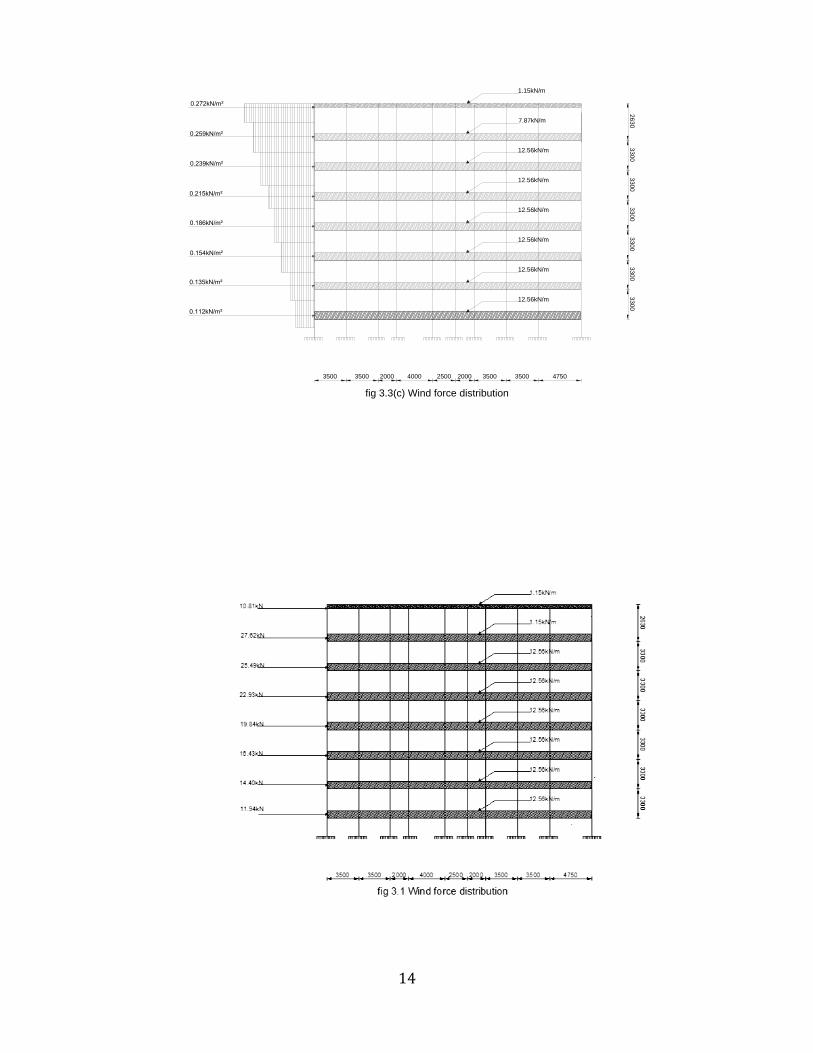
47503500

2630

3300

3300

3300

3300

3300

3300

3500200025004000200035003500

0.112kN/m²

0.135kN/m²

0.154kN/m²

0.186kN/m²

0.215kN/m²

0.239kN/m²

0.259kN/m²

0.272kN/m²

fig 3.3(c) Wind force distribution

1.15kN/m

7.87kN/m

12.56kN/m

12.56kN/m

12.56kN/m

12.56kN/m

12.56kN/m

12.56kN/m

15

3.5 FINITE ELEMENT FORMULATION

Finite Element Method is a numerical procedure for solving engineering problems. We have assumed

linear elastic behavior throughout. The various steps of finite element analysis are:

1. Discretizing the domain: wherein each step involves subdivision of the domain into elements

and nodes. While for discrete systems like trusses and frames where the system is already

discretized up to some extent we obtain exact solutions, for continuous systems like plates and

shells, approximate solutions are obtained.

2. Writing the element stiffness matrices: The element stiffness equations need to bewritten for

each element in the domain. For this we have used MATLAB.

3. Assembling the global stiffness matrix: We have used the direct stiffness approach for this.

4. Applying boundary conditions: The forces, displacements and type of support conditions etc.

are specified.

5. Solving the equations: The global stiffness matrix is partitioned and resulting equations are

solved.

6. Post processing: This is done to obtain additional information like reactions and element forces

and displacements.

The end nodes 1, 2 and 3 are subjected to shear forces ( ) and moment (M1, M2 and M3)

respectively resulting in translation (w1,w2 and w3) and rotation ( ) respectively. This

shows that there are two degrees of freedom per node summing up to four per element. Given that

the elements carry point loads q1 and q2 at the nodes as shown below, then the equilibrium equation

for the system can be written as:

The continuous variable w and its derivative ⁄ denoted by, can be approximated in term of the

nodal values through simple function of the space variable N, known as the

shape function. Thus for each element,

[ ] [

]………………………………...…………...3.8

16

This can be made exact by choosing cubic functions.

{

⁄ )

⁄ )

⁄ )

⁄ )

………………………………….3.9

Substituting the above equation (3.8 and 3.9) and applying Galerkin’s method, we have

∫ [

]

[ ] ∫ [

] ∫ [

] ...........................3.10

Also, by applying Green’s theorem to evaluate the integrals, equation (3.10) becomes

EI

[

⁄ ⁄

⁄

⁄

⁄

⁄

⁄ ⁄

⁄ ⁄

⁄ ⁄

⁄ ⁄

⁄ ⁄ ]

(

) [

]……....3.11

Note that equation (3.11) is only applicable where there are point loads at the nodes.

This can also be written generally as

[ ] ) { }……………………………………………………….3.12

And this form the stiffness equation for the element.

Having define the stiffness matrix for the individual element, the next step is form the global stiffness

matrix

Given that, [ ] ) { }…………………………………………………...….…3.13

Where[ ] is the global stiffness matrix resulting from the assemblage of individual stiffness

matrix.

17

Where ) is the vector representing the degree of freedom at the mesh point. And can be obtained

once [ ] is determined.

Where { }: is the load

The moment can thus be calculated as,

{ } [ ] ) ………………………………………………………..…..3.14

Where [ ] is the function of the flexural rigidity, given by

………………………………………………….…………………..3.15

Likewise the stress could be obtained as

{ } [ ]

⁄ …………………………………………………………….....3.16

Now we are going to apply the above procedure to the structure in consideration.

3.6 FINITE ELEMENT ANALYSIS AND FORMULATION FOR THE SYSTEM

Step 1: Discretising the structure into finite element

Figure 3.4.1 Nodes definition

18

From figure 3.4.1, we could see that there are ninety (90) nodes and one hundred and fifty two (152)

elements in the structure. Which means the number of elemental stiffness matrix to be formed will

be one hundred and fifty two (152). However, this can be reduced by considering the whole structure

as an entity as shown in figure 3.4.2 below.

Figure 3.4.2 Reformed structure

Also, from figure 3.4.2, the number of nodes and elements have been reduced. Which means the

number of elemental stiffness matrix to be formed as automatically reduced. However, the number

of elements can further be reduced for simplicity.This is done byconsidering the structure as a two

element structure (first floor and other floors).Resolving the whole system to determine the moment

and the resultant force (for other floors) which will produce the same effect when placed at the eight

floor as shown in figure 3.4.5.

Taking moment at node 3,

∑

) )+ ) ) )

) )+ )

19

Now to determine a single force P (resultant force) that will act at node 1, we therefore use

∑

) )

⁄

Figure 3.4.3 Diagram showing reformed structure with reactions

20

Figure 3.4.4 Diagram showing the degree of freedom

It has been said earlier that there will be two degree of freedom at each node as shown in figure

3.4.4.The stiffness matrix for the element in local coordinate was found to be

EI

[

⁄ ⁄

⁄

⁄

⁄

⁄

⁄ ⁄

⁄ ⁄

⁄ ⁄

⁄ ⁄

⁄ ⁄ ]

⁄

21

For element 1, node 1-2,L=22.43m

By factorising ,

⁄ [

]

[

)

) ) )

) )

)

) ) )

) ) ]

{

}

[

]{

}

[

]{

}

[ )

) ) )

) )

)

) ) )

) ) ]

{

}

[

]{

}

22

[

]{

}

Assembling the global stiffness matrix

[

]

{

}

Computing the load vector for elements

Element 1,

{

}=

{

⁄

⁄

⁄

⁄ }

=

{

}

={

}

Element 2,

{

}=

{

⁄

⁄

⁄

⁄ }

=

{

}

23

={

}

Now forming the global stiffness matrix for the loads

[

]

Applying boundary conditions

Partitioning the global system at the third row and column

[

]

{

}

[

]

The solution to the problem was solved using MATLAB as shown in appendix A

{

} {

}

24

.

[ ]

=

[ ]

[

]

{

}

[

]

The solution was solved using MATLAB as shown in appendix A

Where R and M are the shear forces and Moments

The result for other storeys can be obtained by interpolation.

[ ]

=

[ ]

[

]

=

[ ]

For reactions For bending moments

25

3.7 SAMPLE SOFTWARE APPLICATION (MIDAS/Gen)

MIDAS/Gen is a program for structural analysis and optimal design in the civil engineering and

architecture domains. The program has been developed so that structural analysis and design can be

accurately completed within the shortest possible time. The name MIDAS/Gen stands for General

structure design. MIDAS/Gen has been developed in Visual C++, an object-oriented programming

language, in the windows environment. The program is remarkably fast and can be easily mastered

for practical applications. By using the elaborately designed GUI (Graphic User Interface) and the

up-to-date graphic display functions, a structural model can be verified at each step of formation and

the results can be directly set into document formats.

3.7.1 Procedures

The steps involved in modelling and analysing the structure (multi-storey building) are as follow:

1. Creating the structural Diagram

2. Defining the Structural Properties

3. Defining the support conditions

4. Defining and Assigning of loads

5. Set analysis Option and run Analysis

6. Display of Desired Result.

1. Creating the structural Diagram

The diagram was created from the Draw tool on the menu bar of the window. The nodes and the

elements were initially created and connected as defined.Prior to the aforementioned steps, the units,

coordinates, grids and views (front view) were defined and the necessary toolbars were made visible.

This is shown in figure 3.5.1

26

Figure 3.5.1 Preliminary setting

The model from the menu bar was clicked, the grid was selected and made active as shown in figure

3.5.2

Figure 3.5.2 Diagram showing the grids

27

The elements and nodes were created by selecting the node and element button from the tree menu.

This was achieved through the selection of translation and extrusion buttons for nodes and elements.

This is shown in figure 3.5.3(a) and (b) below

Figure 3.5.3(a) Extrusion of elements

Figure 3.5.3 (b) Isometric view of the extruded elements

28

2. Defining the Structural Properties

This involves clicking on the menu button and select properties.Define the properties of the structural

elements such as the material, section and thickness. This is shown in figure 3.5.4

Figure 3.5.4 Diagram showing defining of properties

3. Defining the support conditions

After modelling of the shape of the structure the next step was provision of support conditions. In this

project, the lower ends of the columns were fixed. This was executed by highlighting the positions of

the support, the model from main menu was clicked, finally the boundary and support type were

selected. The selected support as shown in figure 3.5.5 became active immediately the process was

completed.

29

Figure 3.5.5 Diagram showing the structure with support conditions

4. Defining and Assigning of loads

This is done by clicking the load from the main menu, select the static load cases and fill the required

information as shown below in figure 3.5.6(a).Prior to this the building data which will automatically

be generated must be confirmed. After the first entry (dead load) the remaining load cases (live and

wind ) can be added by clicking the add button.

Figure 3.5.6(a) Loading data input.

30

Now the self and floor loads need to be defined. This is shown below in figure 3.5.6(b)

Figure 3.5.6 (b) Self weight definition

Figure 3.5.6 (c) Floor load definition

31

Now the defined loads as shown below was assigned on the structural elements accordingly.

.

Figure 3.5.6(c) Assign floor loads

Finally, assign the wind load by selecting the load menu and applied the lateral loads as shown in

figure 3.5.6 (d)

Figure 3.5.6 (d) Assign wind load

32

Note that the loads need to be combined before the analysis is done.

5. Set analysis Option and run Analysis

This is where the structure is subjected to the loading. And it done by clicking the analysis from

the menu and select perform analysis.

Figure 3.5.7 Analysis of the structure

6. Display of Desired Result.

This is the final stage of the whole process where the result will be obtained. This done by clicking the

result from menu bar and select the stresses, reaction and deformation.

33

Figure 3.5.8 Analysis result