A Geometric Comparison of Single Chain Multi-State

Models of Ion Channel Gating

Postprint of article published in: Bull. Math. Biol. 70 (5) (2008) 1503–1524.

Allan R. Willms1

Dept. of Mathematics and StatisticsUniversity of GuelphGuelph, ON N1G 2W1

Canadaph: 519-824-4120 x52736

fax: 519-837-0221AWillms@uoguelph.ca

Dominic Nelson2

Dept. of Mathematics and StatisticsUniversity of GuelphGuelph, ON N1G 2W1

Canada

May 30, 2008

1Corresponding Author2Undergraduate student

Abstract

Multi-state models of ion channel gating have been used extensively, but choosing optimallysmall yet sufficiently complex models to describe particular experimental data remains adifficult task. In order to provide some insight into appropriate model selection, this paperpresents some basic results about the behaviour of solutions of multi-state models, partic-ularly those arranged in a chain formation. Some properties of the eigenvalues and eigen-vectors of constant-rate multi-state models are presented. A geometric description of athree-state chain is given and, in particular, differences between a chain equivalent to anHodgkin–Huxley model and a chain with identical rates are analyzed. One distinguishingfeature between these two types of systems is that decay from the open state in the Hodgkin–Huxley model is dominated by the most negative eigenvalue while the identical rate chaindisplays a mix of modes over all eigenvalues.

Keywords: Multi-state models, Ion channels, Geometric description, Hodgkin–Huxley model,Identical rate chain

1 Introduction

Ion channels are proteins embedded in the membranes of neurons and muscle cells. Theyform a gateable pore which can open to allow the passage of ions, and hence electric chargesin or out of the cell. Many channels are selective to the particular ions they allow topass, and most open or close in response to external stimuli such as the binding of ligandsor the electric field across the cell membrane. Ion channels have received a considerableamount of mathematical treatment since Hodgkin and Huxley (1952) first published theirmodel of sodium and potassium conductance across the giant axon of Loligo. Hodgkin andHuxley modelled the potassium conductance as proportional to x4 where x obeyed a first-order differential equation and represented the probability of a “gating charge” moving intoposition to open the channel. The power four (or, in the case of their sodium conductance,three) was chosen because it accounted for the observed delay in the increase of the currentupon depolarization and as such was a “useful simplification” compared to higher-orderequations (Hodgkin and Huxley, 1952, p. 506). In terms of the “gate” analogy, the powerfour represents four independent gates which must all open (or four gating particles whichmust all dock) for the channel to conduct ions.

Since 1952, the physical view of the ion channel has moved from independent gateswhich open and close to discrete states through which the channel protein progresses as itmoves to a conformation where its pore is open to conduct ions. Mathematical models of ionchannels have, therefore, moved from single first-order Hodgkin–Huxley (HH) type equationsto systems of first-order differential equations where each variable represents the probabilityof being in a specific conformational state. (Of course, an nth order equation is equivalent to asystem of n first order equations, so this type of model was at least contemplated by Hodgkinand Huxley themselves.) Such models are called multi-state models, or Markov models sincethe future state of the channel depends only on the current state, and are represented bysystems of linear equations. Typically, only one state is considered to be open, but modelswith multiple open states, or states with differing conductance levels are also possible. Ashas been pointed out by others and as we describe below, the Hodgkin–Huxley model canbe viewed as a particular multi-state model, and so multi-state models are a generalizationof their original model.

Transitions between states of a multi-state model are governed by rate functions, whichfor voltage-dependent ion channels, are functions of the voltage difference across the mem-brane. Such models can also be used for ligand-dependent channels (Destexhe et al., 1994).Thermodynamic arguments (Eyring et al., 1949; Tsien and Noble, 1969; Hill and Chen, 1972;Hille, 1992) relate the transition between states to either a charge surmounting a free-energybarrier, or rotation of a rigid dipole. In the simplest case where the free energy depends lin-early on the voltage, they predict that the functional forms for the transitions back and forthbetween two states are simple exponentials (given below in Sect. 3) which depend on fourindependent parameters. More parameters arise if more complicated voltage-dependencerelations are used (Destexhe and Huguenard, 2000). Thus, even if every new state is onlyconnected to one other state, every new state added to the model introduces at least fournew parameters.

1

A consequence of using multi-state models is that even with a relatively small number ofstates, the number of free parameters is very large. On the one hand, this means that with theproper choice of parameters and connections between states, the model can replicate nearlyany kinetic observations. On the other hand, the problem of determining an appropriatelysmall model and the optimal parameter values for that model to best fit a given set of data isvery difficult. This problem is compounded by a lack of information. Measurements of ionicconductance through the channel only provide direct information about the open state orstates. The measurement of “gating currents” provides additional information on parametervalues and on the dynamics among closed states, but not to the point of providing a timeseries for each state.

Operationally, the primary means of dealing with this excess of freedom in the modelshas been to restrict state connections and the rate functions in some manner. Typically, thestates are ordered in a partial sequence with each state connected to usually two, sometimesthree, or at most four others. The rate functions are often restricted by dictating that allor a set of the forward rates be identical or integer multiples of each other, and the reverserates similarly (Zagotta et al., 1994b; Roux et al., 1998; Bezanilla, 2000; Bahring et al., 2001;Chanda and Bezanilla, 2002; Piper et al., 2003). Aggregation of similarly behaving statescan also be performed to yield some simplification (Kienker, 1989; Kijima and Kijima, 1997).

Multi-state models are not the only type of model for ion channels. The large number offree parameters associated with multi-state models motivated the development of continuummodels (Levitt, 1989). The technical advance of single-channel recordings has resulted infractal models championed by Liebovitch and others (Liebovitch et al., 1987; Liebovitchand Todorov, 1996; Liebovitch et al., 2001). A review of various stochastic models for ionchannels can be found in Ball and Rice (1992). Nonetheless, multi-state models continue toenjoy considerable use.

This paper presents some basic results about the behaviour of solutions of multi-statemodels, particularly those whose states are arranged in a chain formation, and provides ageometric comparison between a Hodgkin–Huxley type model and other multi-state mod-els. The motivation is to provide insight into some of the properties of these models andconsequently aid in the selection of appropriate models for particular channels.

In Sect. 2, we present some basic results about multi-state models of ion channels regard-ing their equilibria and eigenvalues, and we specialize these results to single chain systemsincluding a chain equivalent to the HH model and a chain with identical forward and back-ward rates. In Sect. 3, we give a geometric description of a three-state model and particularlycompare the behaviour of the HH chain with the identical rate chain. Sect. 4 provides somediscussion.

2 Equilibria and Eigenvalues of Multi-State Models

We are interested in models of ion channel gating where the model states represent differentphysical conformations of the channel protein as it transitions between a non-conducting(closed pore) and conducting (open pore) state. Typically, although not necessarily, onestate, is regarded as the open state, and the remaining states are considered closed. Models

2

could also allow several open states with possibly differing conductance levels. For voltage-gated ion channels, the rates of transition between states depend on the voltage differenceacross the neuronal membrane. For ligand-gated channels, the rates would depend on theabundance of ligand. When the transition rates are constant (experimentally a voltage-clampsituation for voltage-gated channels, or a constant concentration of ligand for ligand-gatedchannels), the models become systems of constant coefficient linear differential equationsand are thus amenable to considerable analysis. In this section, we describe how the modelforms and physical constraints dictate the qualitative behaviour of these models, namely, thesystem has a unique asymptotically stable equilibrium point and all of the eigenvalues arereal. Although these results are generally known and follow from basic analysis, we providethem here for completeness and clarity.

We model the transitions between states as a simple continuous-time Markov processwith n+1 states where xi(t) is the probability of being in state i at time t, i = 0, . . . , n, andρij is the rate at which a channel in state i moves to state j. Let R be the matrix whose ithrow jth column entry is ρij. The governing system is

x′ = Ax, (1)

withA = RT − diag(R1), (2)

where 1 is the column vector of ones in Rn+1, and diag(v) is the diagonal matrix constructed

from the entries of the vector v.The model structure immediately constrains the dynamics. The form of A given in (2)

implies that 1TA = 0, that is, the entries in each column add to zero, thus(

1Tx)′= 0 and,

therefore, 1Tx is a constant for all time. We require the probabilities of being in each stateto add to one, hence we are interested in dynamics on the particular invariant manifold

M ={

x ∈ Rn+1

∣

∣1Tx = 1}

. (3)

In addition, the physical situation imposes several restrictions on the transition rateswhich in turn constrain the dynamics. First, ρij ≥ 0 and ρii = 0. (From the form of A, thisimmediately implies that the non-negative orthant for (1) is invariant.) Secondly, we assumeevery subset of states leads to at least one other state, in other words, no subset of statesis absorptive, and the system does not decompose into two or more disjoint subsystems.Mathematically this assumption is: for each non-empty proper subset P of {0, . . . , n} notall ρij, i ∈ P , j 6∈ P can be zero. This assumption implies, in the case of constant rates,uniqueness of an equilibrium on M in the positive orthant as the following lemma andtheorem show.

Lemma 1 The null space of A is spanned by a vector whose entries are all positive.

Proof: Since 1TA = 0, the null space of A must have dimension at least one. Let x 6= 0 bein the null space of A and suppose there is a non-empty proper subset P of {0, . . . , n} such

3

that xi is positive if and only if i ∈ P . Let S be the selection vector for P , that is, Si = 1 ifi ∈ P and Si = 0 if i 6∈ P . Consider STAx. Using (2) and the fact that Ax = 0, we have

STRTx = STdiag(R1)x

∑

j∈P

n∑

i=0

ρijxi =∑

i∈P

n∑

j=0

ρijxi

∑

j∈P

∑

i 6∈P

ρijxi =∑

i∈P

∑

j 6∈P

ρijxi

Clearly the left side of the above expression is non-positive while the right side is non-negative. Hence equality requires both sides to be zero, but since xi > 0 for i ∈ P , the onlyway the right side can be zero is if ρij = 0 for all i ∈ P and all j 6∈ P which violates thesecond assumption above. We conclude that any non-zero vector x in the null space of Amust either have all entries positive, or all entries non-positive. No two or higher dimensionalsubspace of Rn+1 is contained in this region and every one dimensional subspace contained init necessarily enters the positive orthant. Hence, there must be a vector all of whose entriesare positive which spans the null space of A. �

Theorem 1 There is a unique vector x∗ satisfying Ax∗ = 0 and 1Tx∗ = 1. Furthermore,all entries of x∗ are positive.

Proof: By the previous lemma, there is a vector w, whose entries are all positive, that is abasis for the null space of A. Since Ax∗ = 0, x∗ = cw for some real number c. But 1T cw = 1has the unique solution c = 1/

∑n

i=0 wi which is clearly positive, hence all entries of x∗ arepositive. �

Finally, as a last assumption, we require that at thermodynamic equilibrium there is nonet flow between any two states. This prevents there being a net directional movement ofchannels at equilibrium around a set of states connected in a loop. This latter assumptionis called the law of detailed balance and it may be expressed as

ρijx∗i = ρjix

∗j , ∀i, j ∈ {0, . . . , n}

or equivalently,diag(x∗)R = RTdiag(x∗) (4)

(Fredkin et al., 1985). This final assumption constrains the eigenvalues of A:

Lemma 2 (Fredkin et al., 1985, p. 277) A is real diagonalizable.

Proof: As a consequence of (4), from (2), we have

Adiag(x∗) = diag(x∗)AT .

4

Since all entries of x∗ are positive, we may define the symmetric, invertible matrix W =diag(

√x∗) and thus, multiplying the above by W−1 on both the left and the right gives

W−1AW = WATW−1 = (W−1AW )T .

Therefore A is similar to a real symmetric matrix and thus A is real diagonalizable. �

In particular then, A never has complex eigenvalues. The model form and physical con-straints on the transition rates also imply that n of the real eigenvalues are negative:

Theorem 2 One eigenvalue of A is zero and the remaining n satisfy −2maxi∑n

j=0 ρij ≤λ < 0.

Proof: We have already shown that the null space of A has dimension one, hence exactlyone eigenvalue is zero. Lemma 2 also dictates that the remaining eigenvalues are also real.By a well-known theorem on eigenvalue estimates (Mirsky, 1963, p. 212), all eigenvalues λof A = [aij] must satisfy one of the inequalities

|λ− aii| ≤∑

j 6=i

|aji|, for some i=0, . . . , n.

But by construction of A and since ρij ≥ 0 and ρii = 0, we have∑

j 6=i |aji| = |aii|, andaii = −∑n

j=0 ρij < 0. Thus all but the single zero eigenvalue of A satisfy

−2n

∑

j=0

ρij ≤ λ < 0, for some i = 0, . . . , n. (5)

�

Furthermore, let λ0 = 0 and denote the non-zero eigenvalues of A as λi, i = 1, . . . , n. Besidesthe bounds on the eigenvalues provided by (5), by computing the trace of A, we have

n∑

i=1

λi = −n

∑

i=0

n∑

j=0

ρij. (6)

The preceding results allow us to fully describe the qualitative dynamics on M for (1), inthe case where rates ρij are constants. By Theorem 1, x∗ is a unique fixed point on M . If welet y = x− x∗, the manifold M is given by 1Ty = 0. Since 1 is orthogonal to all vectors inM and since it is a left eigenvector of A corresponding to the zero eigenvalue (1TA = 0), weconclude that the n-dimensional manifold M is precisely the eigenspace of x∗ correspondingto the n negative eigenvalues of A given by Theorem 2. Consequently, for this linear systemrestricted to M , x∗ is globally asymptotically stable, and all of the eigenvalues are real andnegative.

5

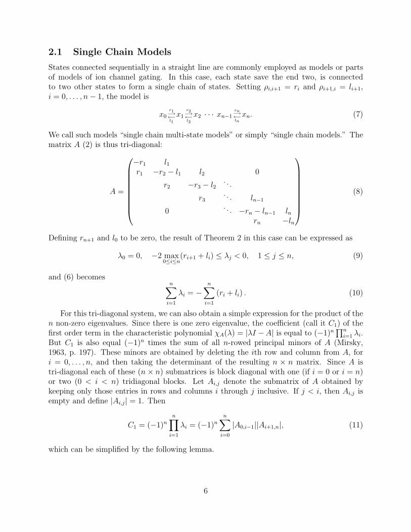
2.1 Single Chain Models

States connected sequentially in a straight line are commonly employed as models or partsof models of ion channel gating. In this case, each state save the end two, is connectedto two other states to form a single chain of states. Setting ρi,i+1 = ri and ρi+1,i = li+1,i = 0, . . . , n− 1, the model is

x0

r1−→

←−

l1

x1

r2−→

←−

l2

x2 · · · xn−1rn−→

←−

ln

xn. (7)

We call such models “single chain multi-state models” or simply “single chain models.” Thematrix A (2) is thus tri-diagonal:

A =

−r1 l1r1 −r2 − l1 l2 0

r2 −r3 − l2. . .

r3. . . ln−1

0. . . −rn − ln−1 ln

rn −ln

(8)

Defining rn+1 and l0 to be zero, the result of Theorem 2 in this case can be expressed as

λ0 = 0, −2 max0≤i≤n

(ri+1 + li) ≤ λj < 0, 1 ≤ j ≤ n, (9)

and (6) becomesn

∑

i=1

λi = −n

∑

i=1

(ri + li) . (10)

For this tri-diagonal system, we can also obtain a simple expression for the product of then non-zero eigenvalues. Since there is one zero eigenvalue, the coefficient (call it C1) of thefirst order term in the characteristic polynomial χA(λ) = |λI −A| is equal to (−1)n

∏n

i=1 λi.But C1 is also equal (−1)n times the sum of all n-rowed principal minors of A (Mirsky,1963, p. 197). These minors are obtained by deleting the ith row and column from A, fori = 0, . . . , n, and then taking the determinant of the resulting n × n matrix. Since A istri-diagonal each of these (n× n) submatrices is block diagonal with one (if i = 0 or i = n)or two (0 < i < n) tridiagonal blocks. Let Ai,j denote the submatrix of A obtained bykeeping only those entries in rows and columns i through j inclusive. If j < i, then Ai,j isempty and define |Ai,j| = 1. Then

C1 = (−1)nn∏

i=1

λi = (−1)nn

∑

i=0

|A0,i−1||Ai+1,n|, (11)

which can be simplified by the following lemma.

6

Lemma 3 For A given by (8),

|A0,i−1| = (−1)ii

∏

j=1

rj, i = 1, . . . , n,

and

|Ai+1,n| = (−1)n−i

n∏

j=i+1

lj, i = 0, . . . , n− 1.

Proof: ForA0,i−1, consecutively applying the row operations “add row j to row j+1” for j =0, . . . , i− 2 yields an upper triangular matrix with diagonal entries −rj, j = 1, . . . , i. Sincethese row operations do not alter the value of the determinant, the result follows. Similarly,consecutively applying the row operations “add row j to row j−1” for j = n, n−1, . . . , i+2to Ai+1,n yields a lower triangular matrix with diagonal entries −lj , j = i + 1, . . . , n whosedeterminant is as specified. �

We can now establish:

Theorem 3 For A given by (8), the non-zero eigenvalues satisfy

n∏

i=1

λi = (−1)nn

∑

i=0

[

i∏

j=1

rj

][

n∏

j=i+1

lj

]

, (12)

where, by definition, we take an empty product to be one.

Proof: The result follows immediately from (11) and Lemma 3. �

2.1.1 Hodgkin–Huxley Type Chains

Now consider a single chain multi-state model where the rates in (7) are given by the specialform ri = (n− i+ 1)α, and li = iβ, i = 1, . . . , n:

x0nα−→

←−

β

x1(n−1)α−→

←−

2β

x2 · · · xn−1α−→

←−

nβ

xn (13)

The governing system of differential equations is

x′j = (n− j + 1)αxj−1 − [(n− j)α + jβ] xj + (j + 1) βxj+1, j = 0, . . . , n, (14)

where x−1 and xn+1 are defined to be zero. By setting

xj =

(

n

j

)

mj(1−m)n−j (15)

it is clear that∑n

j=0 xj =(

m+(1−m))n

= 1. Further, substituting (15) into (14), a straightforward calculation shows that for each j, the differential equation becomes

m′ = α(1−m)− βm. (16)

7

This is the classical Hodgkin–Huxley differential equation for a gate of a voltage-gated ionchannel. Here m represents the probability of the gate being in the open state, and α and βare the rates of opening and closing of the gates, respectively (both depending continuouslyon the voltage). If there are n independent gates in the channel and if g is the maximalconductance of the channel (all gates fully open), then the conductance of the channel isgiven by g = gmn, which is equivalent to saying that xn is the open state in the single chainmulti-state model (14), and all other states are closed. Hodgkin and Huxley used specificforms for how the rate functions depend on the voltage, but we will name any model of theform (14) as an Hodgkin–Huxley type chain, or simply HH chain.

The equivalence between these two models as described above was first noted by Fitzhugh(1965) although with some notational differences, and has been described by others, forexample, Destexhe et al. (1994). Fitzhugh also noted that this equivalence is not dependenton the rates (α and β) being constants. But we stress that the equivalence is only validif the initial condition for x is of the form xj =

(

n

j

)

mj0(1 − m0)

n−j where m0 is the initialvalue for m. Mathematically, this is a substantial restriction on the form of the initialcondition for x, limiting it to a one-dimensional manifold in the n-dimensional manifold M .If this condition is not met, then solutions of (14) do not take the form (15) and clearly then-dimensional Markov system on M has much richer behaviour than the one-dimensionalHH equation. Biologically, however, this restriction is not too severe. In the constant ratefunction (constant voltage) situation, we have established that the multi-state model has aunique globally attractive equilibrium point, x∗. Since (16) clearly has a unique equilibriumgiven by

m∞ =1

1 + β/α,

it immediately follows that x∗ is given by (15) withm = m∞. In other words, the equilibriumof the multi-state model lies on the one dimensional manifold of initial conditions for whichthe multi-state model has solutions given by (15). Consequently, if the voltage is roughlyconstant for a long enough time, the solution of the multi-state system will approach themanifold on which the solutions of the multi-state system are governed by the solutions ofthe single HH differential Eq. (16). If the ion channel’s state can only be altered by variationsin the voltage level, this situation will remain. However, if the ion channel can at sometimesalter its states in a manner where the Markov model need not hold, for example, a fluctuationin the state due to a mechanical stress, then the initial conditions may no longer lie on theequilibrium manifold.

In the case of constant rates, the eigenvalues for (14) are easily obtained. It is not difficultto show that the solution to (16) is

m = m∞ + (m0 −m∞)e−(α+β)t. (17)

From (15), it then immediately follows that the components of x are linear combinations ofterms of the form e−i(α+β)t, for i = 0, . . . , n. From the theory of linear constant coefficientdifferential equations, we are then able to conclude that the eigenvalues of A must be

λi = −i(α + β), i = 0, . . . , n.

8

Therefore, the sum and product of the non-zero eigenvalues for the HH chain are:

n∑

i=1

λi = −(n+ 1)n

2(α + β) (18)

n∏

i=1

λi = (−1)nn! (α + β)n . (19)

2.1.2 Identical Rate Chain

Another commonly employed single chain multi-state model is similar to the Hodgkin–Huxleymodel, but instead of the rates between consecutive states changing linearly, they are all setequal, that is, ri = α, and li = β for i = 1, . . . , n in (7).

x0α−→

←−

β

x1α−→

←−

β

x2 · · · xn−1α−→

←−

β

xn (20)

We call this an Identical Rate (IR) chain. The governing system of differential equations is

x′j = αxj−1 − [α + β] xj + βxj+1, j = 0, . . . , n, (21)

where x−1 and xn+1 are defined to be zero. Although this system appears at least as sim-ple as (14), it does not, unlike the HH system, admit a simple solution dependent on asingle differential equation. Yueh (2005) has recently obtained analytic expressions for theeigenvalues of a generalization of the above system. We can deduce from his work that theeigenvalues for the IR chain are

λ0 = 0, λi = − (α + β) + 2√

αβ cosiπ

(n+ 1), 1 ≤ i ≤ n.

Directly from these, or using (10) and (12), we have:

n∑

i=1

λi = −n (α + β) (22)

n∏

i=1

λi = (−1)nn

∑

i=0

αiβn−i =

(−1)n(n+ 1)αn, α = β

(−1)n(

αn+1−βn+1

α−β

)

, α 6= β(23)

3 Geometrical Description of a Three-State Single Chain

Model

We consider now a three-state single chain model for a voltage-gated ion channel and providea geometrical description of its solutions. Although most models employed for real channelshave more than three states, the geometrical description we provide here (made amenablesince the system restricted to the manifold M is planar) gives some insight into these models

9

and, in particular, to the differences between Hodgkin–Huxley models and more generalmulti-state models. The purpose is to identify distinguishing features of these two types ofmodels. We compare the locations of equilibria of the two models, and the orientation ofthe eigenvectors at these equilibria. Primarily, we are concerned with solutions that startat one equilibrium point and then, due to a sudden voltage jump which alters the system,move to the equilibrium point of the system under the new voltage value. This representsthe typical experimental voltage-clamp situation. In the three-state model, there are justtwo exponential rates of movement (two non-zero eigenvalues), and we compare the relativesizes of these two exponentials in solutions depending on the locations of the pre-step andpost-step equilibrium points. Implications of the results of this section are discussed inSect. 4.

The model for a three-state chain is given by (7) with n = 2 and the governing equationis x′ = Ax, where

A =

−r1 l1 0r1 −r2 − l1 l20 r2 −l2

(24)

Since the dynamics of interest are restricted to the manifold M (x0 + x1 + x2 = 1), it issimpler and sufficient to consider the projection of the system onto the (x0, x2)-plane. Onthis plane, the dynamics are bounded by the coordinate axes and the line x0+x2 = 1; denotethis triangle as ∆. The governing system on ∆ is

[

x0

x2

]′

=

(

−r1 − l1 −l1−r2 −l2 − r2

)[

x0

x2

]

+

[

l1r2

]

. (25)

The rate functions are dependent on the voltage, V . If the voltage is constant, the systemhas a unique equilibrium point

x0 =

(

l1r1

)(

l1r1

+ 1 +r2l2

)−1

=L

L+ 1 +R,

x2 =

(

r2l2

)(

l1r1

+ 1 +r2l2

)−1

=R

L+ 1 +R,

(26)

where for convenience we have defined L = l1/r1 and R = r2/l2. At different constant voltagelevels, the equilibrium will be at different locations in the triangle ∆, forming a curve, C(V ),defined by the parametric Eqs. (26).

We restrict the rate functions by the following two assumptions.

Assumption 1 For fixed σ equal to either +1 or −1,

limV→−σ∞

L = limV→σ∞

R = ∞ and limV→σ∞

L = limV→−σ∞

R = 0. (27)

This assumption dictates that at opposite extreme voltage levels, the equilibrium stateis concentrated in opposite extreme ends of the chain. An activation gate which opensas V increases corresponds to σ = +1, while an inactivation gate which opens as Vdecreases corresponds to σ = −1.

10

Assumption 2dR

dVand

dL

dVare non-zero and of opposite signs.

This assumption provides some monotonicity, in the sense that as the voltage levelmoves from one extreme to another, the equilibrium state moves monotonically awayfrom one extreme end of the chain to the other.

These assumptions are significant and exclude possibilities such as state one being the pre-ferred state at extremely high voltages, or the equilibrium value of state 2 having a non-monotone increase with voltage. Nonetheless, most multi-state models of ion channels satisfythese assumptions.

Within these two assumptions, we further consider several special cases.

Case 1 The model is an Hodgkin–Huxley chain. Thus, r1 = 2r2 = 2α and 2l1 = l2 = 2βwhich yields L = 1/(4R) = β/(2α).

Case 2 The model is an identical rate chain. Thus, r1 = r2 = α and l1 = l2 = β whichyields L = 1/R = β/α.

Case 3 The rate functions are simple exponentials (the most most commonly employedfunctional form for voltage-dependent rates (Zagotta et al., 1994b; Chanda and Bezanilla,2002; Kargol et al., 2002; Piper et al., 2003)) of the form

ri = ri exp (zie0δiV/kT ) ,li = li exp (−zie0(1− δi)V/kT ) ,

i = 1, . . . , n, (28)

where k is the Boltzmann constant, T is the absolute temperature, V is the voltage ofthe inside relative to the outside of the membrane, e0 is the elementary electric charge,zi is the number of positive charges shifted toward the outside of the membrane asthe channel moves from state i to state i + 1, δi is a constant between zero and onewhich represents the relative location of the thermodynamic energy barrier betweenthe two states, and ri and li are constant rates of transition in the absence of an electricpotential. In this case, L = l1

r1exp (−z1e0V/kT ) and R = r2

l2exp (z2e0V/kT ).

It should be noted that while Case 1 and Case 2 are mutually exclusive, Case 3 may or maynot co-exist with either of the first two. For Case 3, Assumptions 1 and 2 are met if andonly if z1 and z2 are of the same sign. For Case 1 and Case 2, the assumptions would besatisfied, for example, if α is a strictly increasing function tending to 0 as V → −∞ and β isa strictly decreasing function tending to 0 as V → ∞. Switching these properties of α andβ would also satisfy these assumptions.

3.1 Shape of the Equilibrium Curve

What is the general shape of the equilibrium curve? Since L and R are necessarily positive,Assumption 1 implies that the equilibrium curve has end points at (x0, x2) = (1, 0) and (0, 1)

11

reached as V → ±∞. From (26), we have

x′0 =

L′(R + 1)− LR′

(L+ 1 +R)2and x′

2 =R′(L+ 1)−RL′

(L+ 1 +R)2,

where the prime denotes differentiation with respect to V . Now since by Assumption 2, L′

and R′ have opposite signs, it immediately follows that the numerators of x′0 and x′

2 are ofopposite sign and are never zero. Therefore, x0 and x2 are invertible functions of V and x2

can also be expressed as a strictly decreasing function of x0 with derivative

dx2

dx0

=x′2

x′0

=R′(L+ 1)−RL′

L′(R + 1)− LR′. (29)

The second derivative of the equilibrium curve, C(V ), is

d2x2

dx20

=1

x′0

(

x′2

x′0

)′

= (L′R′′ − L′′R′) (L+ 1 +R)3 / (L′(R + 1)− LR′)3. (30)

For either an HH type chain or an IR chain, we have that L = b/R for some positive constantb. In these cases, (30) simplifies to

d2x2

dx20

=2R3 (b/R + 1 +R)6

(2/R + 1)3,

which is always positive. For Case 3,

L′R′′ − L′′R′

L′(R + 1)− LR′=

−q1l1r1e−q1V q22

r2l2eq2V − q21

l1r1e−q1V q2

r2l2eq2V

−q1l1r1e−q1V

(

r2l2eq2V + 1

)

− q2l1r2r1 l2

e(q2−q1)V

=q2(q1 + q2)

l2r2e−q2V +

(

q2q1+ 1

) ,

where qi = zie0/kT . Since it has already been established that Assumptions 1 and 2 requirethat z1 and z2 have the same sign, the second derivative is again necessarily positive. Thusin all cases, the equilibrium curve never has an inflection point.

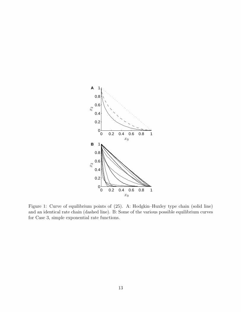
For Hodgkin–Huxley type and identical rate chains, since L and R are inversely related,the equilibrium curve is completely dictated in its shape. These shapes are illustrated inFig. 1A. In contrast, there is a great deal of freedom in the shape of the equilibrium curveif only Case 3 holds, since L and R are independent. Some of the possible shapes are shownin Fig. 1B. This figure illustrates that the steady states for an identical rate chain alwayshave a smaller component of x1, the intermediate state, than a Hodgkin–Huxley type chain.If the voltage is slowly altered so that the system moves from the extreme where x0 = 1to the extreme x2 = 1, then between these two extremes a Hodgkin–Huxley type chain willaccumulate more in the x1 state than an identical rate chain. The straight dotted line inFig. 1 represents x1 = 0; the closer the equilibrium curve is to this line, the more the systembehaves as if there was no intermediate state at all.

12

A

B

0 0.2 0.4 0.6 0.8 10

0.2

0.4

0.6

0.8

1

0 0.2 0.4 0.6 0.8 10

0.2

0.4

0.6

0.8

1

x0

x0

x2

x2

Figure 1: Curve of equilibrium points of (25). A: Hodgkin–Huxley type chain (solid line)and an identical rate chain (dashed line). B: Some of the various possible equilibrium curvesfor Case 3, simple exponential rate functions.

13

3.2 Eigenvectors of the Equilibrium

System (25) will have two negative eigenvalues at the equilibrium point on C, and the relativemagnitude of these two values along with the orientation of the corresponding eigenvectorswill dictate the behaviour of solutions. As we stated earlier, we are interested in solutionswhose initial value is some other point along the curve C. For the Hodgkin–Huxley system,the curve C itself will be the solution, but not for the identical rate system. The solution tothe Hodgkin–Huxley system will have a mixture of both eigenmodes but, as we show in thissubsection, there are initial conditions for which the solution of the identical rate system ispurely along the slow eigenvector, and thus exhibits a single exponential time course.

The eigenvalues of (25) at the equilibrium given by (26) are

λ =1

2

[

− (r1 + l1 + r2 + l2)±√D]

(31)

where

D = (r1 + l1 + r2 + l2)2 − 4

(

(r1 + l1)(r2 + l2)− l1r2)

= (r1 + l1 + r2 + l2)2 − 4(r1r2 + l1l2 + r1l2)

=(

(r1 + l1)− (r2 + l2))2

+ 4l1r2.

(32)

In (31), the plus sign is for the larger (less negative, slower motion) eigenvalue and the minussign gives the smaller (more negative, faster motion) eigenvalue. As we already know, forthe Hodgkin–Huxley type chain, Case 1, these eigenvalues are

λ1 = −(α + β), λ2 = −2(α + β),

and for the identical rate chain, Case 2, they are

λ1 = −(α + β) +√

αβ, λ2 = −(α + β)−√

αβ.

Thus, the IR chain has eigenvalues which are both smaller in magnitude than the HH typechain.

Since the corresponding eigenvectors, v, satisfy either

−(r1 + l1 + λ)v1 − l1v2 = 0 or − r2v1 − (l2 + r2 + λ)v2 = 0,

they may be expressed as either

v =

[

−l112

[

(r1 + l1)− (r2 + l2)±√D]

]

(33)

or

v =

[

12

[

(r2 + l2)− (r1 + l1)±√D]

−r2

]

. (34)

From the third expression for D in (32) it is then clear that the eigenvector corresponding tothe slow motion has negative slope while the eigenvector corresponding to the fast motionhas positive slope. It is therefore, impossible for the fast eigenvector to intersect the strictlydecreasing curve C at any place other than the equilibrium point.

14

0 0.2 0.4 0.6 0.8 10

0.2

0.4

0.6

0.8

1

E

C

x0

x2

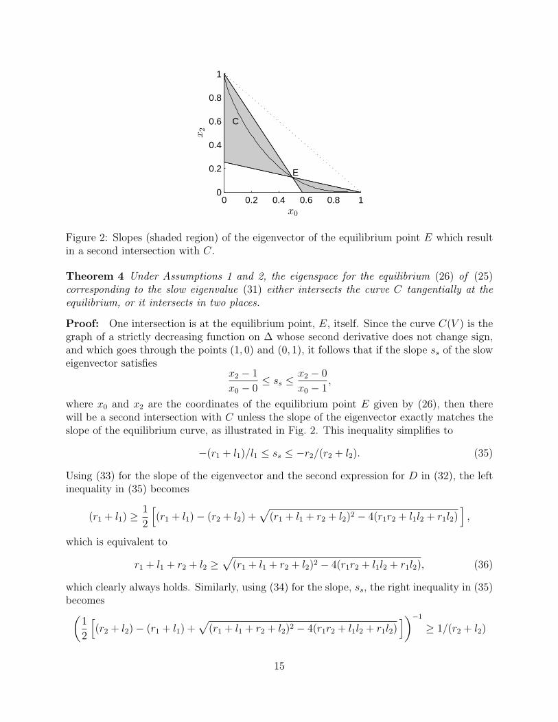
Figure 2: Slopes (shaded region) of the eigenvector of the equilibrium point E which resultin a second intersection with C.

Theorem 4 Under Assumptions 1 and 2, the eigenspace for the equilibrium (26) of (25)corresponding to the slow eigenvalue (31) either intersects the curve C tangentially at theequilibrium, or it intersects in two places.

Proof: One intersection is at the equilibrium point, E, itself. Since the curve C(V ) is thegraph of a strictly decreasing function on ∆ whose second derivative does not change sign,and which goes through the points (1, 0) and (0, 1), it follows that if the slope ss of the sloweigenvector satisfies

x2 − 1

x0 − 0≤ ss ≤

x2 − 0

x0 − 1,

where x0 and x2 are the coordinates of the equilibrium point E given by (26), then therewill be a second intersection with C unless the slope of the eigenvector exactly matches theslope of the equilibrium curve, as illustrated in Fig. 2. This inequality simplifies to

−(r1 + l1)/l1 ≤ ss ≤ −r2/(r2 + l2). (35)

Using (33) for the slope of the eigenvector and the second expression for D in (32), the leftinequality in (35) becomes

(r1 + l1) ≥1

2

[

(r1 + l1)− (r2 + l2) +√

(r1 + l1 + r2 + l2)2 − 4(r1r2 + l1l2 + r1l2)]

,

which is equivalent to

r1 + l1 + r2 + l2 ≥√

(r1 + l1 + r2 + l2)2 − 4(r1r2 + l1l2 + r1l2), (36)

which clearly always holds. Similarly, using (34) for the slope, ss, the right inequality in (35)becomes(

1

2

[

(r2 + l2)− (r1 + l1) +√

(r1 + l1 + r2 + l2)2 − 4(r1r2 + l1l2 + r1l2)]

)−1

≥ 1/(r2 + l2)

15

which also simplifies to (36). �

We have already argued that the equilibrium curve C(V ) is itself a solution of theHodgkin–Huxley system. (More precisely, for a fixed voltage level, C is the union of theequilibrium point and two solutions given by (15)–(16) approaching the equilibrium fromopposite sides.) Here, we verify that the slow eigenvector is in fact tangent to the equilib-rium curve for the HH system. For this system, we have r1 = 2r2 = 2α, and 2l1 = l2 = 2β.Thus, from (33) the slopes of the eigenvectors are

s = −1

2

(

2α

β+ 1

)

−(

α

β+ 2

)

±

√

(

2α

β+ 1 +

α

β+ 2

)2

− 4

(

2α2

β2+ 2 +

4α

β

)

= −1

2

α

β− 1±

√

9

(

α

β+ 1

)2

− 8α2

β2− 8− 16

α

β

= −1

2

α

β− 1±

√

(

α

β+ 1

)2

,

and, therefore,

ss = −α

β, and sf = 1.

Working from (29) and noting that L = β

2α= 1

4Rwe obtain

dx2

dx0

=R′

(

14R

+ 1)

−R(

−R′

4R2

)

(

−R′

4R2

)

(R + 1)− 14RR′

=R′

4R(2 + 4R)

− R′

4R

(

2 + 1R

) = −2R = −α

β.

Similar computations for Case 2, the identical rate chain, where L = β

α= 1

R, yield

ss = −√

α

β, sf =

√

α

β, and

dx2

dx0

= −R(R + 2)

2R + 1= −α(α + 2β)

β(2α + β).

A simple further calculation shows that the slope of the slow eigenvector is less than, equalto, or greater than, the tangent to the equilibrium curve C if and only if α is less than,equal to, or greater than β, respectively. Since by Assumption 2, these two functions haveopposite signed derivatives with respect to V , it follows that there will be one place on theequilibrium curve where the slow eigenvector is tangent to the curve. From (26), it followsthat this point of tangency occurs when x0 = x2. For equilibria on C with x2 > x0 (whichfrom (26) dictates that α > β), the slow eigenvector will have slope greater than the tangentto the curve and so will intersect C to the right of the equilibrium. Conversely, the sloweigenvector emanating from equilibria on C with x2 < x0 will intersect C to the left of theequilibrium. Thus, for every final voltage level (except the one at which α = β), there isalways some initial voltage level such that a voltage jump to the final level from the initiallevel applied to a system at equilibrium will result in a single exponential time course ofthe solution components x0 and x2 toward the new equilibrium point. This feature is adistinguishing feature for identical rate chains compared to Hodgkin–Huxley type chains.

16

3.3 Relative Sizes of the Solution Components

It is informative to look at the relative sizes of the components corresponding to the twoeigenvalues of the solution for x2, comparing the Hodgkin–Huxley type chain with the iden-tical rate chain. We assume that initially the system is maintained at a holding potentialW , and that it is at equilibrium there. Thus the initial condition is given by (26) where thefunctions are evaluated at W . At time zero, the voltage is instantaneously changed to V sothat the globally attractive equilibrium point is given by (26) with the functions evaluatedat V . We assume that x2 is the only open state, and it is the only measurable quantity.(If one is measuring ionic currents only, then this is the case; however, information about acertain linear combination of the states xi can be obtained by measuring gating currents.)The solution for x2 is of the form

x2(t) = aeλ1t + beλ2t + c, (37)

where λ1 is the slow eigenvalue and λ2 the fast one. We are interested in the ratio p = |b/a|.The relevant equation to be solved is

[

x0(W )x2(W )

]

=

[

1/ss 1/sf1 1

] [

ab

]

+

[

x0(V )x2(V )

]

. (38)

Solving the above for a and b, we obtain

[

ab

]

=1

ss − sf

[

−sfss sssfss −sf

] [

x0(W )− x0(V )x2(W )− x2(V )

]

,

thus,

p =

∣

∣

∣

∣

b

a

∣

∣

∣

∣

=

∣

∣

∣

∣

∣

(x0(W )− x0(V ))− 1ss(x2(W )− x2(V ))

(x0(W )− x0(V ))− 1sf(x2(W )− x2(V ))

∣

∣

∣

∣

∣

.

For an HH type chain, Case 1, after some algebra, the ratio p becomes

pHH =|Q(V )−Q(W )|

2Q(V )(

1 +Q(W )) ,

where Q = α/β. For the IR chain, Case 2, the ratio is

pIR =

∣

∣

∣

∣

∣

(

Q(V ) +Q(W ) + 1)(√

Q(V )− 1)

−Q(V )Q(W ) + 1(

Q(V ) +Q(W ) + 1)(√

Q(V ) + 1)

+Q(V )Q(W )− 1

∣

∣

∣

∣

∣

.

For both Case 1 and Case 2, the ratio x2/x0 at equilibrium is given by Q2. Plots of thesurfaces p for both cases as a function of x2(V )/x0(V ) and x2(W )/x0(W ) (on a log scale)are shown in Fig. 3. Note that for the Hodgkin–Huxley type chain, plotted in Fig. 3A, thefast component approaches zero along the diagonal since the slow eigenvector is tangent tothe equilibrium curve and the start and end points are moving together along this curve asthe diagonal is approached. When the end ratio x2(V )/x0(V ) is larger than the initial ratio

17

A B

C D

−4 −2 0 2 4−4−20

240

1

2

−4 −2 0 2 4−4−20

240

0.5

1

−5 −4 −3 −2 −1 0 1 2 3 4 50

0.2

0.4

0.6

0.8

1

−5 −4 −3 −2 −1 0 1 2 3 4 50

0.5

1

1.5

2

log x2(W )x0(W )

log x2(W )x0(W )

log x2(V )x0(V )

log x2(V )x0(V )

log x2(V )x0(V )

log x2(V )x0(V )

pp

pp

x2(W )x0(W )

= 10−4 x2(W )x0(W )

= 104

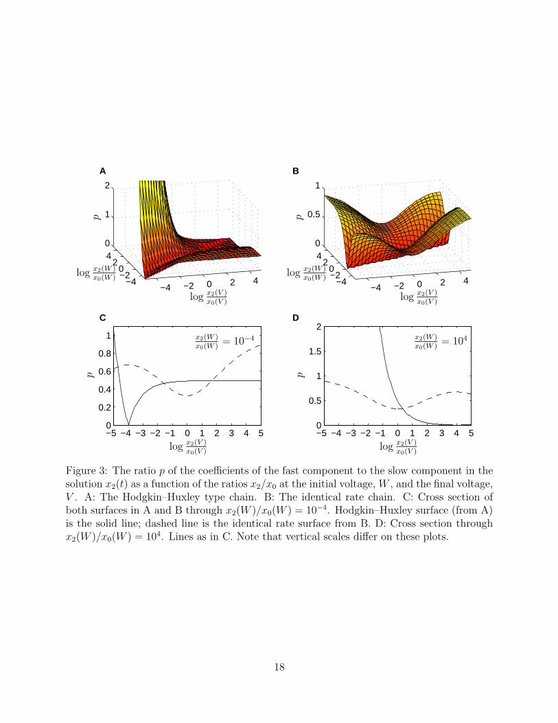
Figure 3: The ratio p of the coefficients of the fast component to the slow component in thesolution x2(t) as a function of the ratios x2/x0 at the initial voltage, W , and the final voltage,V . A: The Hodgkin–Huxley type chain. B: The identical rate chain. C: Cross section ofboth surfaces in A and B through x2(W )/x0(W ) = 10−4. Hodgkin–Huxley surface (from A)is the solid line; dashed line is the identical rate surface from B. D: Cross section throughx2(W )/x0(W ) = 104. Lines as in C. Note that vertical scales differ on these plots.

18

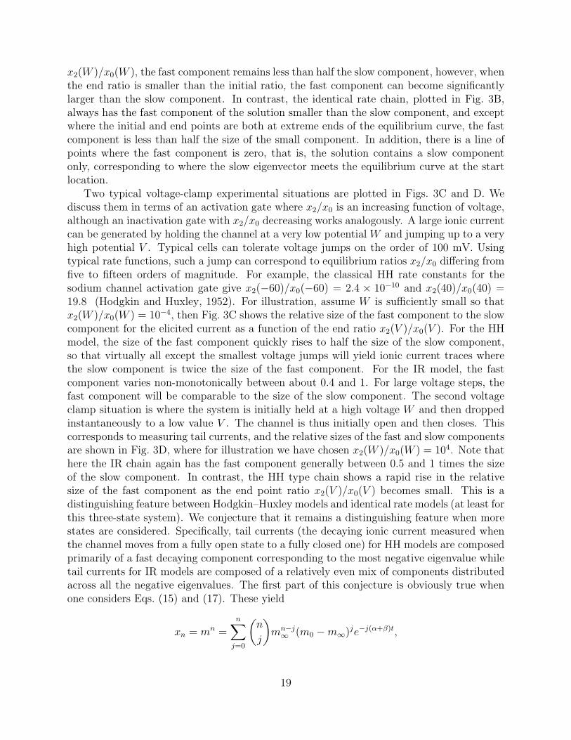
x2(W )/x0(W ), the fast component remains less than half the slow component, however, whenthe end ratio is smaller than the initial ratio, the fast component can become significantlylarger than the slow component. In contrast, the identical rate chain, plotted in Fig. 3B,always has the fast component of the solution smaller than the slow component, and exceptwhere the initial and end points are both at extreme ends of the equilibrium curve, the fastcomponent is less than half the size of the small component. In addition, there is a line ofpoints where the fast component is zero, that is, the solution contains a slow componentonly, corresponding to where the slow eigenvector meets the equilibrium curve at the startlocation.

Two typical voltage-clamp experimental situations are plotted in Figs. 3C and D. Wediscuss them in terms of an activation gate where x2/x0 is an increasing function of voltage,although an inactivation gate with x2/x0 decreasing works analogously. A large ionic currentcan be generated by holding the channel at a very low potential W and jumping up to a veryhigh potential V . Typical cells can tolerate voltage jumps on the order of 100 mV. Usingtypical rate functions, such a jump can correspond to equilibrium ratios x2/x0 differing fromfive to fifteen orders of magnitude. For example, the classical HH rate constants for thesodium channel activation gate give x2(−60)/x0(−60) = 2.4 × 10−10 and x2(40)/x0(40) =19.8 (Hodgkin and Huxley, 1952). For illustration, assume W is sufficiently small so thatx2(W )/x0(W ) = 10−4, then Fig. 3C shows the relative size of the fast component to the slowcomponent for the elicited current as a function of the end ratio x2(V )/x0(V ). For the HHmodel, the size of the fast component quickly rises to half the size of the slow component,so that virtually all except the smallest voltage jumps will yield ionic current traces wherethe slow component is twice the size of the fast component. For the IR model, the fastcomponent varies non-monotonically between about 0.4 and 1. For large voltage steps, thefast component will be comparable to the size of the slow component. The second voltageclamp situation is where the system is initially held at a high voltage W and then droppedinstantaneously to a low value V . The channel is thus initially open and then closes. Thiscorresponds to measuring tail currents, and the relative sizes of the fast and slow componentsare shown in Fig. 3D, where for illustration we have chosen x2(W )/x0(W ) = 104. Note thathere the IR chain again has the fast component generally between 0.5 and 1 times the sizeof the slow component. In contrast, the HH type chain shows a rapid rise in the relativesize of the fast component as the end point ratio x2(V )/x0(V ) becomes small. This is adistinguishing feature between Hodgkin–Huxley models and identical rate models (at least forthis three-state system). We conjecture that it remains a distinguishing feature when morestates are considered. Specifically, tail currents (the decaying ionic current measured whenthe channel moves from a fully open state to a fully closed one) for HH models are composedprimarily of a fast decaying component corresponding to the most negative eigenvalue whiletail currents for IR models are composed of a relatively even mix of components distributedacross all the negative eigenvalues. The first part of this conjecture is obviously true whenone considers Eqs. (15) and (17). These yield

xn = mn =n

∑

j=0

(

n

j

)

mn−j∞ (m0 −m∞)je−j(α+β)t,

19

so that the ratio of the component of xn corresponding to the most negative eigenvalue,−n(α + β), to the component corresponding to the eigenvalue −j(α + β), 1 ≤ j < n, is

(m0 −m∞)n(

n

j

)

(m0 −m∞)jmn−j∞

=1(

n

j

)

(

m0

m∞

− 1

)n−j

.

Therefore, as m∞ → 0 (which implies xn(V )/x0(V ) → 0), this ratio is unbounded.

4 Discussion

When developing multi-state models of ion channels constructed of several (typically four)membrane spanning subunits, it has been commonly assumed that the symmetry of thephysical channel should be reflected in some symmetry of the model. If each subunit canhave a “closed” and an “open” state, then four subunits generate five different states for thechannel (zero through four subunits “open”). For this reason, chains of five states with thelast state open, or leading to subsequent states from which the channel opens are common(Bezanilla, 2000). In order to reduce the number of free parameters in the models, thesechains are often constructed as Hodgkin–Huxley type chains or identical rate chains. Ourgeometric analysis of the three-state chains suggests that Hodgkin–Huxley type chains andidentical rate chains are distinguishable in their movement from a fully open to a fully closedstate. Currents of the former type decay primarily through the fastest mode (most negativeeigenvalue) while currents of the latter appear to decay with a relatively even mix of fastand slower modes. As has been observed by others, for example Zagotta et al. (1994a), tailcurrents for some channels display a nearly single exponential time course of deactivation.This suggests an HH type chain in the activation pathway, however, models of specific ionchannels often involve inactivation or passage from the open state to states not directlyin the activation pathway (Zagotta et al., 1994b; Bezanilla, 2000). These additional stateshave the potential of significantly altering the kinetics of the open state. Nonetheless, anunderstanding of differences in the single chain systems we have described here is an aid inunderstanding the behaviour of more complicated models.

We have concentrated on single chain models, although the first results of Sect. 2 areapplicable to all multi-state models. If a channel also undergoes inactivation, then it can bemodelled as a single chain system with additional closed states beyond the open state. Inother words, the chain has n+ 1 states but the open state is not the last one, rather one inthe middle. Some of our results are applicable to these models, but usually such chains arenot HH type or IR chains, or not completely so. More commonly, inactivation involves theaddition of states which generate potential loops in the network. For example, a multi-statemodel that is equivalent to the classical Hodgkin–Huxley model for the sodium conductancein the squid giant axon is

x04αm−→

←−

βm

x13αm−→

←−

2βm

x22αm−→

←−

3βm

x3αm−→

←−

4βm

x4

αh ↑↓ βh αh ↑↓ βh αh ↑↓ βh αh ↑↓ βh αh ↑↓ βh

x54αm−→

←−

βm

x63αm−→

←−

2βm

x72αm−→

←−

3βm

x8αm−→

←−

4βm

x9

20

where x4 is the open state and the m and h subscripts refer to the activation and inactivationrate functions. Other models including inactivation tend to have less symmetry than theabove model but also introduce loop connections between a number of states (Bezanilla, 2000;Zagotta et al., 1994b). More work needs to be done on such models to get a fundamentalunderstanding of their behaviour.

In the three-state IR model, we showed that (except in the case where the final conditionis x0 = x2) there is always an intersection of the slow eigenvector with the curve of equilibria.This means that in the typical situation, where the initial condition lies on the equilibriumcurve and a sudden change in the voltage is applied, for each final voltage level there willalways be a particular initial voltage level such that the solution for this case is a singleexponential corresponding to the slow eigenvalue. This is another distinguishing featurebetween the three-state identical rate chain and the three state Hodgkin–Huxley chain; theHH chain always has multi-exponential solutions involving all the eigenvalues. In a higherdimensional setting, the generalization of this result is not immediately clear. Geometrically,the equilibrium curve and the eigenspace for the slow eigenvector are one-dimensional man-ifolds and so their meeting in a space of higher than two dimensions is not expected. Thus,even for a four-state IR model a single exponential solution connecting two points on theequilibrium curve is not likely. However, it is not clear whether the structure of the problemwith the symmetries of the IR chain might not dictate that the eigenspace must intersectthe equilibrium curve. More work in this direction is required.

Acknowledgements

This research was partly supported by the Natural Sciences and Engineering Research Coun-cil of Canada. D.N. acknowledges the support of the University of Guelph through an Un-dergraduate Research Assistantship.

References

Bahring, R., Boland, L. M., Varghese, A., Gebauer, M., Pongs, O., 2001. Kinetic analysis ofopen- and closed-state inactivation transitions in human Kv4.2 A-type potassium channels.J. Physiol. 535, 65–81.

Ball, F. G., Rice, J. A., 1992. Stochastic models for ion channels: Introduction and bibliog-raphy. Math. Biosci. 112, 189–206.

Bezanilla, F., 2000. The voltage sensor in voltage-dependent ion channels. Physiol. Rev. 80,555–592.

Chanda, B., Bezanilla, F., 2002. Tracking voltage-dependent conformational changes in skele-tal muscle sodium channel during activation. J. Gen. Physiol. 120, 629–645.

Destexhe, A., Huguenard, J. R., 2000. Nonlinear thermodynamic models of voltage-dependent currents. J. Comp. Neurosci. 9, 259–270.

21

Destexhe, A., Mainen, Z. F., Sejnowski, T. J., 1994. Synthesis of models for excitable mem-branes, synaptic transmission and neuromodulation using a common kinetic formalism. J.Comp. Neurosci. 1, 195–230.

Eyring, H., Lumry, R., Woodbury, J. W., 1949. Some applications of modern rate theory tophysiological systems. Record Chem. Prog. 10, 100–114.

Fitzhugh, R., 1965. A kinetic model of the conductance changes in nerve membrane. J. Cell.Comp. Physiol. 66, 111–115.

Fredkin, D. R., Montal, M., Rice, J. A., 1985. Identification of aggregated Markovian models:Application to the nicotinic acetylcholine receptor. In: Cam, L. M. L., Olshen, R. A. (Eds.),Proceedings of the Berkeley Conference in Honor of Jerzy Neyman and Jack Kiefer. Vol. 1.Institute of Mathematical Statistics, Wadsworth Advanced Books & Software, Monterey,CA, pp. 269–289.

Hill, T. L., Chen, Y. D., 1972. On the theory of ion transport across nerve membranes. VI.free energy and activation free energies of conformational change. Proc. Natl. Acad. Sci.USA 69, 1723–1726.

Hille, B., 1992. Ionic Channels of Excitable Membranes. Sinauer, Sunderland, MA.

Hodgkin, A. L., Huxley, A. F., 1952. A quantitative description of membrane current andits application to conduction and excitation in nerve. J. Physiol. Lond. 117, 500–544.

Kargol, A., Smith, B., Millonas, M. M., 2002. Applications of nonequilibrium response spec-troscopy to the study of channel gating. Experimental design and optimization. J. Theor.Biol. 218, 239–258.

Kienker, P., 1989. Equivalence of aggregated Markov models of ion-channel gating. Proc.Royal Soc. London B 236, 269–309.

Kijima, H., Kijima, S., 1997. Theoretical approaches to ion channel dynamics and the first-order reaction. Prog. Cell Res. 6, 295–304.

Levitt, D. G., 1989. Continuum model of voltage-dependent gating. Biophys. J. 55, 489–498.

Liebovitch, L. S., Fischbarg, J., Koniarek, J. P., 1987. Ion channel kinetics: A model basedon fractal scaling rather than multistate Markov processes. Math. Biosci. 84, 37–68.

Liebovitch, L. S., Scheurle, D., Rusek, M., Zochowski, M., 2001. Fractal methods to analyzeion channel kinetics. Methods 24, 359–375.

Liebovitch, L. S., Todorov, A. T., 1996. Using fractals and nonlinear dynamics to determinethe physical properties of ion channel proteins. Crit. Rev. in Neurobiol. 10, 169–187.

Mirsky, L., 1963. An Introduction to Linear Algebra. Oxford, Clarendon Press, London.

22

Piper, D. R., Varghese, A., Sanguinetti, M. C., Tristani-Firouzi, M., 2003. Gating currentsassociated with intramembrane charge displacement in HERG potassium channels. PNAS100, 10534–10539.

Roux, M. J., Olcese, R., Toro, L., Bezanilla, F., Stefani, E., 1998. Fast inactivation in ShakerK+ channels. J. Gen. Physiol. 111, 625–638.

Tsien, R. W., Noble, D., 1969. A transition state theory approach to the kinetics of conduc-tances in excitable membranes. J. Membr. Biol. 1, 248–273.

Yueh, W.-C., 2005. Eigenvalues of several tridiagonal matrices. Appl. Math. E-Notes 5, 66–74.

Zagotta, W. N., Hoshi, T., Dittman, J., Aldrich, R. W., 1994a. Shaker potassium channelgating II: Transitions in the activation pathway. J. Gen. Physiol. 103, 279–319.

Zagotta, W. N., Hoshi, T., Dittman, J., Aldrich, R. W., 1994b. Shaker potassium channelgating III: Evaluation of kinetic models for activation. J. Gen. Physiol. 103, 321–362.

23