William M. Humphreys, Jr. Thomas F. Brooks …...William M. Humphreys, Jr. Thomas F. Brooks William...

N i

/V/'J

/_A 5 _-/'_'_ _ /_" _-_>_- 207321

AIAA 98-0471

Design and Use of MicrophoneDirectional Arrays forAeroacoustic Measurements

William M. Humphreys, Jr.Thomas F. BrooksWilliam W. Hunter, Jr.Kristine R. Meadows

NASA Langley Research CenterHampton, VA 23681-0001

36st Aerospace Sciences

Meeting & Exhibit

January 12-15, 1998 / Reno, NV

For permission to copy or republish, contact the American Institute of Aeronautics and Astronautics1801 Alexander Bell Drive, Suite 500, Reston, Virginia 20191-4344

https://ntrs.nasa.gov/search.jsp?R=19980037002 2020-03-14T08:55:46+00:00Z

AIAA-98-0471

DESIGN AND USE OF MICROPHONE DIRECTIONAL ARRAYS

FOR AEROACOUSTIC MEASUREMENTS

William M. Humphreys, Jr.*Thomas F. Brooks t

William W. Hunter, Jr.*Kristine R. Meadows _

Fluid Mechanics and Acoustics Division

NASA Langley Research CenterHampton, Virginia 23681-0001

Abstract

An overview of the development of two microphone

directional arrays for aeroacoustic testing is presented.These arrays were specifically developed to measureairframe noise in the NASA Langley Quiet FlowFacility. A large aperture directional array using 35flush-mounted microphones was constructed to obtainhigh resolution noise localization maps aroundairframe models. This array possesses a maximumdiagonal aperture size of 34 inches. A uniquelogarithmic spiral layout design was chosen for thetargeted frequency range of 2-30 kHz. Complementingthe large array is a small aperture directional army,constructed to obtain spectra and dircctivityinformation from regions on the model. This array,

possessing 33 microphones with a maximum diagonalaperture size of 7.76 inches, is easily moved about themodel in elevation and azimuth. Custom microphone

shading algorithms have been developed to provide afrequency- and position-invariant sensing area from10-40 kHz with an overall targeted frequency range for

the array of 5-60 kHz. Both arrays are employed inacoustic measurements of a 6 percent of full scaleairframe model consisting of a main element NACA632-215 wing section with a 30 percent chord half-span

*Research Scientist, Measurement Science and Technology

Branch, Senior Member AIAA.

*Senior Research Scientist, Aeroacoustics Branch, Assc_ate

Fellow AIAA.

*Senior Research Scientist, Measurement Science and

Technology Branch.

1Researdt Sdentlst, Aeroa_ustics Branch, Member AIAA.

Copyright O1998 bythe American Institute of_cs and

Astronautics, Inc. No copyright is asserted in the United States

under Title 17, U.S. Code. The U.S. Gov_t has a royalty-flee

liceme to exercise all rights under the copyright claimed herein for

govenunent _. All other rights are reserved by the copyrightOWt'ler.

flap. Representative data obtained from thesemeasurements is presented, along with details of thearray calibration and data post-p_ing procedures.

Nomenclature

Superscripto

AC

coD

fd

kM

MoPy

t

1/

w

W(k, £, £o)

source location

shearlayer amplitude correction,dBconstant

speedofsound,IVsec

SADA clusteraperture,seeeqn.(16)

steeringmatrix,seccqn.(13)

frequency, cycles/scc

cross spectral matrixcross spectra between ithandj _microphones, see eqn. (6)wavenumber (=c0/co), ft"ltotal number of microphones in arrayMath number (--v/co)pressure, Pascalsradialdistance, fl

time, sec

velocity,ft/sec

arrayshadingmatrix

microphonedusterweighting

theoreticalarrayresponseat

wavenumberk,dB,seeeqn.(4)

spectralwindow weightingconstantke_FFT datablockforis'andjth

microphones

location,fl

locationofphasecenterofarray,R,

see eqn. (3)

American Institute of Aeronauticsand Astronautics

G

C0

coat

acoustic wavelength, R

SADA array weighting controlfrequency, rad/sec

shear layer phase correction for co,radians,see eqns.(9)and(13)

Introduction

Over the past several years a growing need hasemerged for accurate and robust noise measurementinstrumentation in aerospace research facilities. Thisneed is partly driven by research programs such as theNASA Advanced Subsonic Technology (AST)

Program, which has set as one of itsgoalsthe

achievingofa greaterthan 10 dB reductionintotal

aircraft effective perceived noiseby the year 2000(referenced to levels measured in 1992). This goalrequires the collection of experimental databases ofvarious noise generation mechanisms from whichaccurate and efficient noise prediction tools can bedeveloped to guide noise reduction design. Recently,emphasis has been placed on the measurement andmodeling of airframe noise, defined as the non-propulsive component of aircraft noise which is due tounsteady flow about the airframe components (flaps,slats, undercarriage, etc.).

One of the databases desired by computationalairframe noise modelers is farfield noise data measured

on various baseline and modified aircraft components.

Traditional single microphone measurements of thisnoise have been hampered by poor signal-to-noisecharacteristics, spurring the development of a varietyof new measurement techniques. Early techniques

employed the concept of an "acoustic mirror", where alarge concave elliptic mirror and an associatedmicrophone were positioned in the acoustic far field. 1"_

Such mL,xors were capable of locating individual soundsources accurately, but suffered the drawback ofrequiring mechanical movement to determine sourcedistributions around models. The mirrors also became

excessively large when measurements of lower

frequencies (< 2 kHz) were required. Nevertheless,such mirrors continue to have applicability in some ofthe larger research facilities. 4

In addition to acoustic mirrors, distributions ofindividual microphones have been employed todetermineairframenoisesourcecharacteristics.In

particular,such systemshave provenvaluablein the

understandingof single-elementairfoilselfnoise.56

Whilenot strictlyconsidereda directionalarray(the

outputsof allmicrophoneswere not combinedas in

beamforming),such systems capitalizedon the

amplitudeand phaserelationshipsbetweenclustersof

microphones. As such, they can be considered one ofthe precursors to the current generation of microphonedirectional arrays.

Modem microphone directional arrays foraeruaconstic research have as their origin early radioand radarantennaarraysand U.S.Navy hydrophone

arrays (used for the detection of submarines as early asWorld War 11)._'s Soderman and Noble were amongthe first researchers to adapt this earlier work foraeroaconstics when they constructed a one-dimensionalend-fire array to evaluate jet noise in the NASA Ames40- by 80-foot Wind Tunnel. 9"1° At the same timeBillingsley and Kinns constructed a one-dimensionallinear array of microphones for real-time sound sourcelocation on full-size jet engines, n More recently _ch

directional arrays have been extended to include two-dimensional microphone layouts with the work ofBrooks, Marcelini and Pope 12"13, Underbrink and

Dougherty TM, and Watts and Mosher. 15q6Two different state-of-the-art, two-dimensional

microphone directional arrays are described in thispaper. These are designed to provide broadband sourcelocalization and directivity information needed tocharacterizeairframe noise and noise reduction

concepts. Both arrays have been successfidly used bythe authors to obtain data for a wing / flap model. 17

This paper expands on the previouswork by providingdetailed descriptions of the design and construction ofthe two directional arrays. The philosophysurrounding their design as well as development ofunique data processing algorithms to allow accuratenoisespectraand source imagesto be obtainedare

discussed.Finally, severalrepresentativeexamplesofdata collected with the instruments are illustrated.

Directional Array Development

Concept

The basic principleof a microphonedirectional

array can be simply illustrated.Assume a simple

monochromatic acoustic point source is located in

quiescent space at location _ (see Figure 1). Asolution for r>O representing the propagation of apressure wave radially in all directions is given by

p(r,t) = Cei(_'-k') (1)r

where C is a constant, r is the radial distance from the

source origin, co is the frequency of the wave, and k isthe corresponding wavenumber. Assume now that anarray of M microphones is placed a finite distance from

2American Institute of Aeronautics and Astronautics

the source. Each microphone senses a slightlydifferent phase-s_ wave.form depending on itsdistance from the source. The pressure pro(t) measuredat the m-th microphone is denoted as

C ya,(t-_)p.(t) = --e Co

rm(2)

where rm represents the distance from the location tothe m-th microphone. The (t-rJCo) term is theretarded time from the source to the microphone. Inorder to focus on a source, the individual microphoneoutputs can be phase shifted an amount equal to theirpropagation delay and then summed together (orstacked). This yields a single output signal for thearray in a process commonly referred to as delay-and-sum beamforming. By adjusting the propagationdelays, one is able to electronically steer the array topoints in space, selecting regions of interest toascertain noise production while providing noiserejection not found in individual microphonemeasurements. This steering can provide the samecapability as the earlier acoustic mirror techniques butwithout the necessity of physically moving the array tomeasure source distributions.

Array Response

The phase center of the array is defined as_s

1 M

m=-I

(3)

Using this, the ideal array response for a simple sourcecan be expressed as

M ¥oW(k,£,£°) -- _ wm-- e j_[(?-')-(r_-r-)]

(4)

where x is an arbitrary Cartesian location in space to

which the array is electronically steered, £°is the

source location, r ° and r om are the distances from the

source to _¢and the m-th microphone, respectively,

and r and r., are the distances from the steering

location to _¢and the microphone. The term w m

represents a microphone weighting factor which can beused to modify the array response.

The array response is normally expressed in

decibels referenced to the level obtained at ,_o :

(5)

This response is plotted as a contour map with contour

level proportional to O_(x-), representing the

computation of equation (5) over a large number of

steering locations lying on a surface a finite distancefrom the array. Such plots represent the spatial

filtering of the array graphically at wavenumber k, andallows one to examine the beamwidth and lobestructure.

Array Desien Criteria for AirframeNoise Measurements

Test Model and Facility: The test program isintended to investigate the mechanisms of soundgeneration on high-lift wing configurations. InFigure 2, the test model apparatus and the LargeAperture Directional Array, to be discussed, axe shownmounted in the Langley Quiet Flow Facility (QFF).The QFF is a quiet open-jet facility designedspecifically for anechoic acoustic testing. 19 For the

present airframe model testing, a 2 by 3-footrectangular open-jet nozzle is employed. The model isa NACA 632-215 main element airfoil with a 30percent chord half-span Fowler flap. In the photo, themodel is visible through the Plexiglas windows locatedon the side plates. The model section is approximately

6 percent of a full-scale configuration, with a mainelement chord length of 16 inches, a flap chord lengthof 4.5 inches, and a full span of 36 inches. The mainelement and flap are fully instrumented with staticpressure ports and unsteady pressure transducers. To

hold the model in place, the vertical side plates arefastened rigidly to the side plate supports of the nozzle.Appropriate acoustic foam treatments are applied to alledges and supports to reduce acoustic reflections fromthese surfaces. More model and facility details can befound in Reference 17.

Array Design Criteria: In choosing an arraydesign, specifically the microphone layout with respectto the noise source to be studied, one must be aware ofthe character of the source distributions. The basic

delay-and-sum beamformer procedure, describedabove, renders an array output which assumes anysingle source to be an omni-dircctional simplemonopole, or any distribution of sources to be that ofincoherent (uncorrelated) simple monopoles. But,when the sources are multi-pole and/or coherent over a


spatialsourcedistribution,the noiseis not omni-directional.Forsuchdirectional sources, variations innoise field coherence, amplitude, and phase can occurover the face of the array. Major difficulties occurwhen the directivity has an oscillatory sweeping orrotational phase behavior. Still, even when sourcedirectivity is stationary, which is assumed to be thecase for the airframe noise problem, spatial variationscan cause moderate to severe errors in source

amplitude, resolution, and localization. This isbecause the phase variations are interpreted as retardedtime delays, and amplitude/coherence variationsmodify the relative contribution of each microphone tothe array output. Indeed, the effect of limited spatial

coherence for the noise directivity is to effectivelybreak an array with too large an aperture (overall widthof the array of microphones) into a group of smallersub-arrays whose individual steered output spectra aresummed together. This is "pressure-squared"summing rather than the desired "linear-pressure"summing (operation indicated by equation (4)), therebymodifying the desired "design" characteristics of the

array. To avoid such errors, all array microphonesshould be placed within approximately the same sourcedirectivity (producing generally a small array), whereamplitude and phase appear as ff the source were

omni-direotional. However, as will be seen, this designconstraint cannot always be fully met and still have thedesired array resolution at the frequencies of interest.

Airframe noise measurements present an arraydesign challenge in that not only is source directivityinformation required (necessitating the use of a smallaperture array to satisfy the concerns discussed above),but also accurate localization of the source distributions

is desired down to the order of the smallest wavelengthof interest, typically one to two tenths of an inch. Thislatter need requires that the array aperture be large inorder to minimize the array beamwidth, defined hereas the width across the main response lobe over whichthe sensing level is within a given dB level from thepeak level. However, the required spectra anddirectivity information dictate the use of a small arrayaperture to ensure that all microphones are atapproximately the same directivity angle.

R was decided to address the two conflictingaperture requirements through the construction of twoarray designs. A Large Aperture Directional Array(LADA) was designed to produce high spatialresolution (narrow beamwidth) noise source

localization maps over a defined surface on the model.To obtain quantitative spectra and directivityinformation, particularly for the dominant noise

sources identified with the LADA, a Small ApertureDirectional Array (SADA) was also designed. This

array was constructed to be movable about the model inboth elevation and azimuth, as opposed to the LADAwhich was fixed in location. The SADA results can

also be used to evaluate the degree of directivityuniformity the LADA encounters to add confidence tothe LADA results.

Description of Two Directional Arrays

Large Averture Directional Array (LADA): TheLADA is shown to the left in Figure 2, on the pressureside of the model, positioned 4 feet from the mid-spanof the airfoil main element trailing edge. A 4-footdiameter fiberglass panel provides a flat surface toflush mount all microphones. The panel is attached toa pan-tilt unit secured to a rigid tripod support. Thisallows precise alignment changes in the elevation andazimuth of the face of the array. A small laser diode

pointer is place at _,, corresponding to the center of

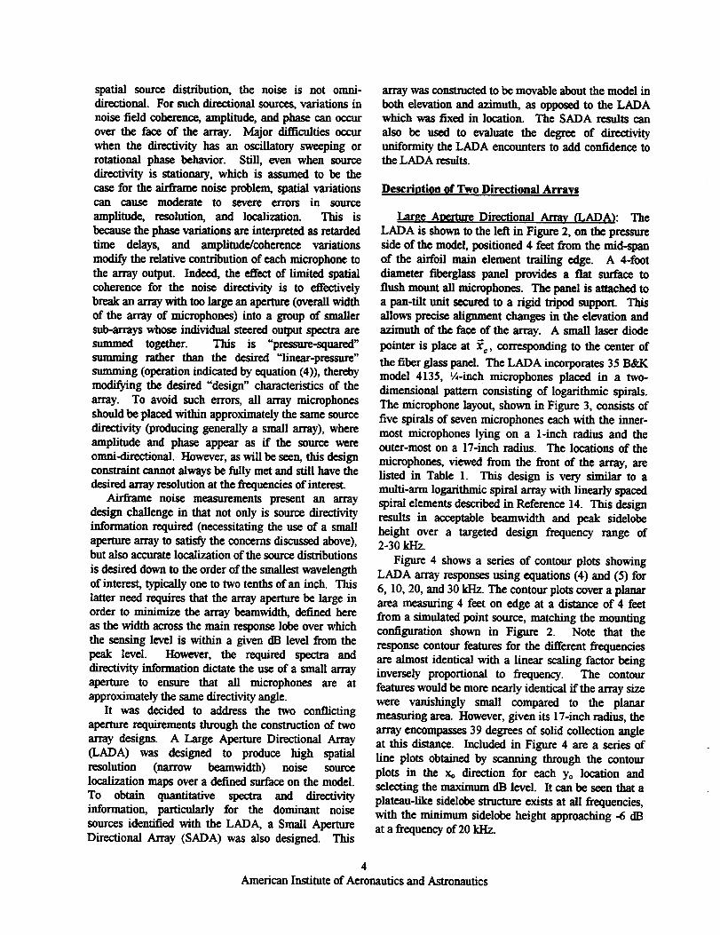
the fiber glass panel. The LADA incorporates 35 B&Kmodel 4135, _A-inch microphones placed in a two-dimensional pattern consisting of logarithmic spirals.The microphone layout, shown in Figure 3, consists offive spirals of seven microphones each with the inner-most microphones lying on a 1-inch radius and theouter-most on a 17-inch radius. The locations of the

microphones, viewed from the front of the array, arelisted in Table 1. This design is very similar to amulti-arm logarithmic spiral array with linearly spacedspiral elements described in Reference 14. This designresults in acceptable beamwidth and peak sidelobeheight over a targeted design frequency range of2-30 kHz.

Figure 4 shows a series of contour plots showingLADA array responses using equations (4) and (5) for6, 10, 20, and 30 kHz. The contour plots cover a planararea measuring 4 feet on edge at a distance of 4 feetfrom a simulated point source, matching the mountingconfiguration shown in Figure 2. Note that theresponse contour features for the different frequenciesarc almost identical with a linear scaling factor beinginversely proportional to frequency. The contourfeatures would be more nearly identical ffthe array sizewere vanishingly small compared to the planarmeasuring area. However, given its 17-inch radius, the

array encompasses 39 degrees of solid collection angleat this distance. Included in Figure 4 are a series of

line plots obtained by scanning through the contourplots in the xo direction for each 3,0 location andselecting the maximum dB level. It can be seen that a

plateau-like sidelobe structure exists at all frequencies,with the minimum sidelobe height approaching -6 dBat a frequency of 20 kHz.

4

American Institute of Aeronautics and Astronautics

A study of the beamwidth characteristics of theLADA can be achieved by observing a series of arrayresponses for a number of frequencies spanning arange of 2-30 kHz and measuring the width of themain lobe at various dB levels. Figure 5 shows a

family of curves where the main lobe width ismeasured at the -0.5, -1, -3, and -6 dB level. It can beseen from the curves that a typical -3 dB beamwidthfor the LADA is approximately 1.5 times the source

wavelength.

SmallApertureDirectionalArray(SADA): The

SADA isdesignedtocomplementthe capabilitiesof

the LADA by providingdirectivityand spectral

informationasafunctionofpositionaroundthemodel.

The apertureofthearrayiskeptsmallwiththeintent

to keep all microphones in the array withinapproximately the same source directivity regardless ofelevation or azimuth position. The array pattern whichwas chosen to achieve this can be seen in Figure 6,with the locations of the microphones given in Table 2.The SADA consists of 33 B&K model 4133, 1/8-inch

microphoneswith ¼-inch preamplifiersprojectingfrom an acousticallytreatedaluminum flame. The

arraypatternincorporatesfourirregularcirclesofeight

microphoneseachwithone microphoneplacedat xc,

correspondingtothecenterofthearray.Eachcircleistwice the diameter of the circle it encloses. The

maximum radiusofthearmy is3.89inches,givingthe

SADA only5.25% ofthesurfaceareaoftheLADA.Two smalllaserdiodepointersareincorporatedinto

the arraymount on oppositesidesof the center

microphone for use in alignment.The SADA is mounted on a pivotal boom designed

to allow it to be positioned to a wide range of elevationand azimuth angleswhile maintaininga constantdistancetothecenterofthetrailingedgeofthemain

elementairfoil(anassumednoiseproductionregion).

This is achievedby maintainingthe boom's pivot

centeratthetrailingedgeofthemain elementairfoil.

Rotationoftheboom isperformedusingprecisionDC

servo rotation stages mounted on the outer edges of the

side plates holding the model and boom. This isillustratedin Figure7, which shows the SADA

mountedintheQFF on thesuctionsideofan airframenoisemodel at a 5-footworkingdistance.At this

distancethearrayencompasses7.5 degreesof solid

collectionangle.

Figure8 shows a seriesof contourplotsshowingSADA array responses using equations (4) and (5) for10, 20, 30 and 40 kHz. Subsequently, a processing

procedure is used to maintain constant spatialresolution, independent of frequency; however, this is

not done in the calculations of Figure 8. The contour

plots cover an area measuring 4 feet on edge at adistance of 5 feet from a simulated point source,

matching the mounting configuration shown inFigure 7. A series of line plots obtained from thecontour plots in a process similar to that for the LADAare also shown in Figure 8. It can be seen that the

sidelobe patterns again exhibit a plateau-like structureat all frequencies, with the maximum sidelobe levelapproaching -8 dB at a frequency of 40 kHz.

A study of the beamwidth characteristics of theSADA can be performed similarly to that for the

LADA by observing a series of array l"¢sponses over afrequency range and measuring the width of the mainlobe at various dB levels. Figure 9 shows such a

beamwidth plot. A family of curves is shown wherethe main lobe width is measured at the -0.5, -1, -3, and-6 dB level. It can be seenfrom these curves that a

typical 3 dB beamwidth for the SADA isapproximately 11 times the source wavelength. It willbe seen subsequently that this beamwidth can beradically altered through the use of microphone

shading (or weighting).

Measurement System

Data Acquisition:The dataacquisition/ analysis

systememployed for both arraysis illustratedin

Figure 10. Acquisition hardware consists of a NEFF495 transient data recorder which is controlled by a

DEC AXP3400 workstation. Sampling rate iscontrolledby an externalclock operatingat142.857kHz. The maximum allowableclockrateisI

MI-Iz. The use of an external clock allows

simultaneous acquisition with other instrumentationsuchasthe model unsteady surface pressuresensors,asdescribed in Reference 17. The NEFF system

incorporates 36 12-bit (including sign bit) acquisitionchannels with each channel possessing a 4 megabyte

buffer, allowing up to 2 million 2-byte samples to becollected per acquisition. The signals from eachmicrophone channel are conditioned by passing themthrough high pass filters set to 300 Hz (to remove DC,60Hz linenoise,and low frequencyinterferencenoise)

and through anti-aliasing filters set at 50 kI-Izwhich issubstantially below the 71.43 kHz Nyquist frequency.

Custom software is used to control all aspects of thedata acquisition. The output files generated by the

acquisition system are written in NetCDF format toprovideplatform-independentstorageof the data,afeaturemandated by the distributed data analysissystem. 2° The NetCDF files are archived on the NASALangley Distributed Mass Storage Subsystem for post-test retrieval and processing. 21


A typical acquisition run consists of collecting 36channels (array microphones pins additional referencemicrophones) of data under no flow conditions. This isfollowed by the actual data nm under a specific flow orcalibration condition. As will be seen, _ecwa obtainedfrom the background runs are subtracted from spectraobtained from data runs to remove the noise floor inthe measurements.

Data Analysis: It was desired to build a highly

distributed processing configuration to handle theproblem of array analysis given the volume of datainvolved (greater than 500 Gbytes) and the amount oftime required to process a single test point of data fromstart to finish (typically 30-60 minutes per set on a200-MHz Pentium-Pro machine). There are a number

of various platforms and operating systems used in theprocessing of the array data, including a cluster ofthree 200-MHz NT-based Pentium-Pro workstations, a

500-MHz Alpha workstation running UNIX, and theLangley SP2 supercluster consisting of 48 IBMRS/6000 workstations. This heterogeneous cluster ofhardware systems is controlled from a single Pentium-Pro workstation using a custom control panel programand a series of device independent configuration filesreadable by the individual processing codes located oneach of the various hardware platforms.

Data Post-Processing Procedure

Processing steps common to both arrays include theconstruction of cross spectral matrices from the rawtime data and the calculation of amplitude and time

delay corrections to account for shear layer refraction.Classical beamformer processing algorithms areutilized in the generation of noise images, spectra, anddirectivity information. In addition, the SADAprocessing incorporates a unique shading algorithm

which provides a constant beamwidth independent offrequency.

Computation of Cross Spectral Matrices: AnM byM cross spectral matrix, where M is the totalnumber of microphones in the array, is firstconstructed for each data set (both background and_e component test condition). The formation ofthe individual matrix elements is achieved through theuse of Fast Fourier Transforms (FFT). This is done

after convening the raw data to engineering units(Pascals) using sensitivity data based on a microphonecalibration using a frequency of 1 kHz. Each channelof engineering unit data is then segmented into a seriesof non-overlapping blocks each containing 8192samples, yielding a frequency resolution of 17.45 I-Izfor the 142.857 H-Iz acquisition sampling rate. Using

a Hamming window, each of these blocks of data isFourier transformed into the frequency domain. Theindividual upper triangular matrix elements plus thediagonal (representing auto spectra for each arraymicrophone) are formed by computing thecorresponding block-averaged cross spectra from thefrequency data using

= G22 • :

*°

(6a)

with

N

l zt=l[X_(f)Xit(f) ]=(6b)

where W_is the data window weighting constant, N isthe number of blocks of data, and A_"represents an FFTdata block. The lower triangular elements of thematrix are formed by taking the complex conjugates ofthe upper triangular elements (allowed because thecross spectral matrix is Hermitian).

All cross spectral matrix elements are employed insubsequent processing, with no modification of thediagonal terms. Note that for in-flow arrays, thediagonal terms can be removed to improve the spectraldynamic range by subtracting off seLf-noise dominatedauto-spectra during the beamforming process, asdescribed in References 14 through 16. However, forthe airframe noise measurements described here, this

step was not required since all array microphones areoutside of the flow.

3-D Shear Layer Refraction Correction: Testing inan open-jet facility requires that the effect of the shearlayer on the propagation of the noise (both intensityand retarded time) from sources located in the jet tomicrophones located outside the jet be accounted for.The first challenge was to develop a technique fordealing with the highly three dimensional, curvedshear layer present in the installation. The approachtaken was to acquire five-hole pitot probemeasurements on both the pressure and suction sides ofthe airframe model to map out the velocity field. Theshear layer position was defined to be the half meanvelocity position. This data was then fitted with athree dimensional surface to provide a continuousrepresentation of the shear layer for each of the flowconditions examined. With the shear layer positiondefined, amplitude and phase corrections were


determinedusingthe approachof SctdinkerandAmiet= andAmie_.

Thekeyto findingthe retarded time and phasecorrections is to find the intersection of the source ray

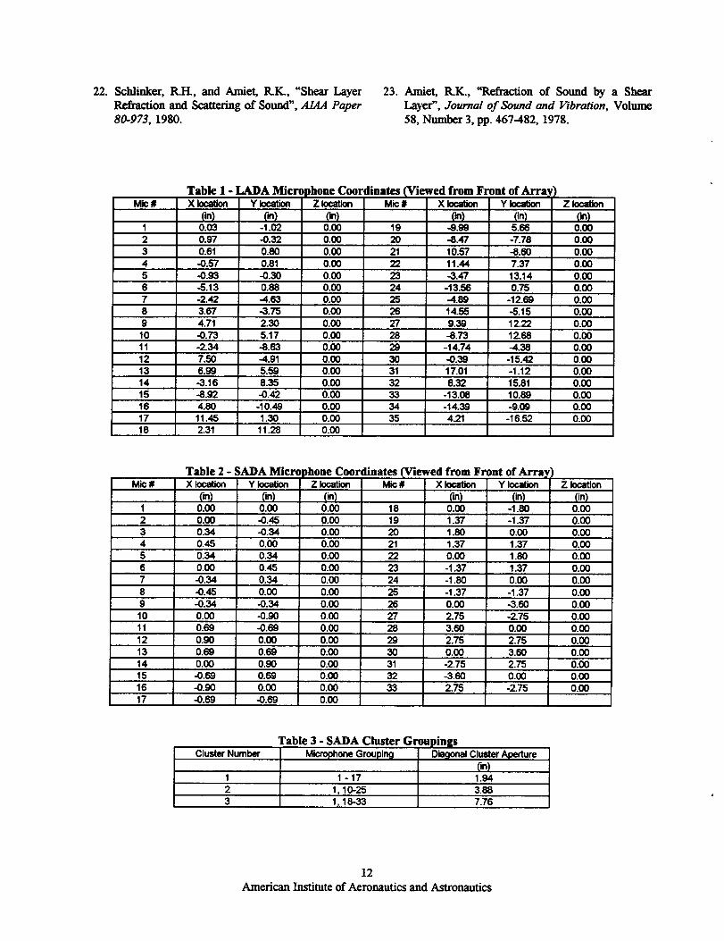
path with the shear layer, as illustrated in Figure 11.An iterative process is used, using the followingrelationship between the source emission angle, qh, the

ray angle, 0, and the free jet Mach number, Mo

tan(O) = sin(_,_)Mo +cos(¢,_) (7)

and SneU's law

cos(_h)cos(q,2) =

1+ Mo cos(_] ) (8)

where the subscripts 1 and 2 refer to angles inside andoutside of the jet, respectively, and the sound speedsinside and outside the jet are assumed equal. Once theray path-shear layer intersection is known, the retardedtime difference and hence the phase can be computedfrom

k co ) (9)

where r_=r_+r2 is the wavefront travel distance(relative to the convecting flow inside the je0, and r=i¢

is the line-of-sight distance from the source to themicrophone.

The amplitude corrections are based upon analysisof a rectangular shear layer. There are two correctionsprovided in Reference 22, namely a thick shear layer(high frequency) correction and a thin shear layer 0owfrequency) correction. The appropriate correction isdetermined by the ratio of the source acousticwavelength to the shear layer thickness. Theassumption in developing the thick shear layercorrection is that the shear layer is sufficiently thick for

geometricalacousticsto apply so that (1) the acousticenergy is conserved along the ray tube, and (2) soundpressure is the result of outgoing waves only sincereflections are absent in the geometrical acousticslimit. As supplied in References 22 and 23, the ratio ofthe corrected to measured sound pressure formicrophone m, including the astigmatism and distancecorrection, is found to be

".'_w2 ,',"_ _in(,,2)P= (10)

with

= 3/(1_ Mo c0s(_2))2 _ c0s2(_2 )

sin 0_cO_1 --

sin _2

6 2 = E/ I3]h -1 +1r_c sin 0_c

(II)

wherepc is the correctedpressure,]7= is the measuredpressure,h is the distance from source to shear layer,and 0.,_ is the measured angle of the microphonerelative to the flow direction.

For the low frequency correction, the reflected waveamplitude cannot be neglected when the wavelength isof the same length as the shear layer thickness. In this

case the amplitude correction is found to be

_ Pc _] 2

P=

[_@_ + (1- Mo cos(¢,O)21 (12)

Examples of the calibration and use of the shearcorrection algorithms are shown subsequently.

Beamforming: A classical beamforming approachis used for the analysis which eliminates instabilitiesand potential matrix singularity problems found inadaptive techniques. The basic procedure consists ofelectronically steering the array to a predefined seriesof locations in space, as shown in Figure 12. Theselocations define a plane which can be positioned in anyorientation in front of the array. For each selected

steering location, a steering matrix containing oneentry for each microphone in the array is computed asfollows:

(13)

where x is the distance from the steering location toeach microphone, Am is the shear layer amplitudecorrection for microphone m using either equation (10)


or (12), and oJdt_,s,_, is the shear layer phasecorrection for microphone m at frequency oJ. Thefactor (r°/r, °) is included to normalize the amplitude

An, to that of the array xc position. Using

equation (13) and the cross spectral matrix computedp_ciously, the steered array output power spectnLm atthe steering location is obtained via

P(_) =M" (14)

where the T denotes the conjugate transpose of thematrix. Note that a background subtraction process isexplicitly denoted in equation (14). The backgroundspectra is that obtained without tunnel flow, where theacquisition system noise dominates the recordedoutput. The division by the number of microphones Mserves to reference the array output spectrum levels toequivalent single microphone output levels.Equation(14) represents the steered response powerspectrum over the full range of single narrowbandfrequencies. If a wider bandwidth is desired (such asan Octave Band), the power (pressure-squared values)of the narrowbands is summed. Note that wider

bandwidths are not formed prior to the completion ofthe vectorial (or complex) operations of equation (14).This prevents possible significant bias errors insumming across phase-shifted cross spectral bands.

SADA Shading Algorithm: The use of the SADAfor directivity and spectral measurements requires thatthe beamwidth he invariant under steering angle andfrequency changes, thereby providing a constantsensing area over noise source regions. The method

used to accomplish this is similar to previoustechniques described in Reference 12 and 13. TheSADA microphones are divided into three clusterscontaining 17 microphones each. These clusters alongwith their maximum diagonal aperture sizes are shownin Table 3. Each cluster exhibits the same directional

characteristics for a given wavenumber-length productkD_, where k is the wavenumber and D, is the diagonaldistance between the elements of the n-th cluster. The

method used to achieve the invariant sensing areaconsists of shading (or weighting) the array clusters asa function of frequency. The microphone clustershadings are calculated as follows:

w t =0 ]w 2 =0

w 3 =1

0-1<0 and ty2 <0

W 1 = 0 -0.875

W 2 = 1-- 0 0.875

w3=0

wl=0

W2 ---- 0-0.875

W3 = 1-- 0-O.875

w_=l

W2 =0

w 3 =0

0 <o-_ <1

0<or 2 <1

0-1>1 and 0-2 > 1

(15)

with the shading coefficients defined by

kD2 - kDo_=

0-2=(16)

The value of kD0 for this study is 36.38, correspondingto frequencies of 10, 20, and 40 kHz for clusters 3, 2,and 1, respectively (assuming a speed of sound of1126 fl/sec). This causes the SADA to yield the sameeffective resolution for all frequencies hetween 10 and40 kHz, with smooth blending among frequencies.The exponent of the coefficients, 0.875, was found todiffer slightly from the array of References 12 and 13.

Figure 13 illustrates modified theoretical array

responses for the SADA for frequencies of 10, 12.5, 15and 17.5 kHz, using equations (4) and (5) with the

shadings of equation (15) substituted for thew,_ term.

Comparing the responses with those shown inFigure 8, note that the responses for 10, 20, and40 kHz are now identical, as are the ones for 12.5 and

25, 15 and 30, and 17.5 and 35 kHz. This clearlyillustrates the fiequency-invariant main and side lobestructure now exhibited by the array. Figure 14 showsa beamwidth plot for the shaded array. At higherfrequencies the beamwidth, while invariant, now takeson the value exhibited at the kDs wavenumber-lengthproduct. In a sense the higher frequency beamwidthshave been sacrificed to achieve frequency invariance.This is an acceptable trade-off; however, since accuratesource directivity data can only be obtained over abroad frequency range ff the sensing area of the arrayis held constant.

To extract noise spectra and directivity from dataobtained with the SADA, the classical beamfonningtechnique is employed with minor variations. First, asingle steering location is chosen for the array, whichis itself positioned at various elevation and azimuth


angles with respect to the model. A modified versionof equation (14) is used to compute the weightedsteered response power for the array at the fixedsteering location via

= M_.. W m

rail (17)

where ]_ is a row matrix containing the set of

shadings computed in equation (15). The sum over themicrophone shading terms in the denominator isobtained fzom equation (15) as a function of frequency(this sum always equals 17 for the present SADAapplication). Note that this formulation of thebeamformer equation is identical to that for the LADA

ffone assumes an identity matrix for W.

Array Calibration and Applications

Careful calibrations are conducted for both arraysystems. These tests axe designed to check fordeviations between experimental and theoretical arrayresponses which can be attributed to microphonesystem response differences, installation effects, orproblems in the data analysis algorithms.

Injection Calibration: Injection calibrations areperformed for the SADA. These calibrations consist ofinserting a known signal simultaneously into allmicrophone channels in order to detect microphonesensitivity and phase drift. Both pure tones and whitenoise are used. This is accomplished without physicaldisruption of the system. Inspection of cross spectralphase between all pairs of microphones allowsdiscrepancies to be easily identified and corrected.Also, sensitivity drift can be corrected without the need

to perform a full microphone calibration before eachrun. Nevertheless, standard SADA microphonecalibrations are also performed daily because of readyaccessibility.

Isolated Point Source: A series of static calibration

tests are performed by placing an isolated point sourcedirectly in front of the array at the operational workingdistance (4 feet for the LADA, 5 feet for the SADA).The point source consists of a tube with one or moreacoustic drivers mounted on the back end. The openend of the tube is intended to provide an omni-directional sound source. Noise measurementsare

obtainedacrossa broadfrequencybandthoughtheuse

of white noise. These are compared with

corresponding theoretical array responses usingequations (4) and (5).

Figure 15 shows a series of LADA point source noiseimages taken at identical frequencies to the theoreticalones shown in Figure 4. Figure 16 shows thecorresponding measured beamwidths which can becompared with Figure 5. At the higher frequenciessome discrepancieswere indicatedbetween the

theoretical and experimentalsidelobe shapes (mostlikelydue to installationcifccts);however, the

measuredbeamwidthsand peak sidelobclevelsagree

wellwiththeory.Figures17 and 18 show a seriesof

SADA noise images and beamwidth line plots

correspondingtotheblendedtheoreticalonesshown in

Figures 13 and 14, respectively.The shading

algorithmisseentobevalidated.

In-Situ Point Source: In addition to the static

calibrations using an isolated point source, tests areconductedusingthepointsourcemountedintheQFF

atthemidpointofthetrailingedgeofthemainclementairfoil.Thesemeasurementsinclude:

• Background acquisition runs for no tunnel airflow.The corresponding spectra is subtracted from theother spectra to remove the noise floor, asdescribed previonsly.

• Acquisition runs with no flow and point sourceturned on to verify processing acau_cy and theeffect of the test apparatus on the acoustic field.

• Acquisition runs with flow and point sourceoperating to evaluate the shear layer correctionalgorithms.

Figure 19 shows a series of noise image maps takenwith the SADA on the pressure side of the model foran elevationangleof 107 degreesand an azimuth

angle of zero degrees. At this location the face of the

array is parallel to the chord of the main elementairfoil. Figure 19(a) shows a photograph of the pointsource mounted in the QFF pointing toward thepressure side of the model. Figure 19Co) shows a30-kHz noise image map of the point source under noflow conditions. Figure 19(c) shows a 30-kHz noiseimage map for the point source operating in aMach 0.17 flow with no shear layer correction applied,while Figure 19(d) shows a similar map withcorrections. Notice that the apparent location of thesource moves approximately 3 inches downstream ofits actual position without shear layer correctionsapplied. The shear layer algorithm returns the sourceto its proper position, as verified by the no flow case.Other SADA elevation angles, producing larger

9

AmericanInstitute of Aeronauticsand Astronautics

position corrections, also find success using thesealgorithms.

Test Application

LADA Measurements: Acoustic noise image mapsare obtained by steering the LADA over a planeparallel to the main element chord on the modelpressure side. Because of limitations in the dataacquisition process in the early test stages of theprogram (of which this particular LADA data wasobtained), background noise spectra have not beensubtracted. However, the effect of background noisewas determined to be negligible for these results.Figure 20 shows typical acoustic image maps taken atfrequencies of 5, 8, 12.5, and 20 kHz. The flow isfrom bottom to top and an outline of the wing and flapprovide a reference for the noise sources that arepredominant. Note that the location and strength ofthe sources are dependent on frequency, with the leveldiminishing with frequency.

The benefits of using a larger aperture withcorresponding narrow beamwidth can be seen inFigure 21. This figure shows the position of the locallydominant noise source location, defined by the centroidof the source on the image maps in Figure 20. Thisfigure shows that along the flap-side edge, a trendexists for the lower frequency sound sources to belocated near the flap trailing edge with the sourcelocation moving to the flap mid chord and flap mainelement juncture at higher frequencies. Suchinformation is only obtainable using an array with asufficiently large aperture size and correspondinglynarrow beamwidth.

SADA Measurements: Figure 22 shows the SADA

elevation angles which were employed for directivitystudies in the QFF. Figure 23 shows flap edge spectrataken at an elevation angle of 107 degrees. The SADAazimuth angle is at zero degrees, corresponding to theplane of the flap side edge surface. The model flapangle condition is 29 degrees. The array is focused onthe flap region, which for this flap angle is by far themost intense noise producing region. Shown on theplot, along with the SADA beamformed-outputspectrum, is the spectra obtained from a singlemicrophone in the array. The difference in levelsbetween these represents the removal of unwantednoise emanating from regions other than those presentat the steering location. As previously indicated, theSADA spectrum represents that noise emitted from aregion of constant size for frequencies between 10 and40 H-Iz. At lower frequencies, the noise emission

region measured is larger; for higher frequencies, theregion is smaller.

Figure 24 shows the elevation angle sourcedirectivity in terms of a series of noise spectra obtainedfor the SADA at a number of elevation angles aboutthe model. The model flap angle is now 39 degrees.With the exception of the most downstream position,the spectra are within 2 to 3 dB of one another forfrequencies from 10-30 kHz. Larger deviations in

directivity occur over the lower and upper frequenciesdue to differences in source characteristics, asdescribed in Reference 17.

It is noted that the LADA's 39 degrees of solidcollection angle sets well within the SADA elevationangle range shown here. The degree of directivityuniformity found over the 10-30 kI-Iz range offrequencies suggests that measurements with theLADA should have quantitative accuracy, in additionto it having source positioning accuracy. This is true,as long as the azimuthal directivity (not determined forthis paper) is likewise uniform and that the spatialsource-noise coherence is high. As previouslyindicated, any lack of spatial uniformity over the arraymicrophones would effectively shade the microphone'sresponse in the beamforming and, thus, would changethe array response characteristics.

Summary,

This paper presents an overview of the design andconstruction of two complementary microphonedirectional arrays used for aeroacoustic testing. ALarge Aperture Directional Array (LADA) has beenconstructed to obtain high resolution noise localizationmaps. A Small Aperture Directional Array (SADA)has also been made to be moved about the model tO

provide localized spectra and directivity from selectednoise source regions. Calibration tests havedemonstrated their accuracy and fimctionality. Botharrays have been used to successfully measure the far

field acoustics on a main element / half-span flapmodel. The LADA was able to detect small changes inlocation of dominant noise sources emanating from theflap edge region, while the SADA was able to obtainspectra and directivity measurements from this region.

Acknowledgments

The authors wish to acknowledge Dave Devilbiss ofLockheed-Martin and Stuart Pope of ComputerSciences Corporation for data processing and softwaredevelopment support. The authors also gratefullyacknowledge Phil Grauberger and Ron Verbapen ofWyle Laboratories for data acquisition system support.

10


References

Kendall, J.M., Jr., "Airframe Noise Measurements

by Acoustic Imaging", A/AA Paper 77-55, AIAA15 _ Aerospace Sciences Meeting, Los Angeles,

CA, Jannary, 1977.

. Grosche, F.R., Stiewitt, H., and Binder, B.,"Acoustic Wind-Tunnel Measurements with a

Highly Directional Microphone", A/AA Journal,

Vohune 15, Number 11, pp. 1590-1596, 1977.

. Sehlinker, R.H., "Airfoil Trailing Edge Noise

Measurements With a Directional Microphone",AIAA Paper 77-1269, 4_ AIAA Aeroacoustics

Conference, Atlanta, GA, October, 1977.

. Grosche, F.R., Schneider, G., and Stiewitt, H.,

"Wind Tunnel Experiments on Airframe Noise

Sources of Transport Aircraft", A/AA Paper 97-1642, 3_ AIAA/CEAS Aeroacoustics Conference,

Atlanta, GA, May, 1997.

5. Brooks, T.F., Marcolini, M.A., Pope, D.S.,

"Airfoil Trailing-Edge Flow Measurements",

AZ4A Journal, Volume 24, Number 8, pp. 1245-

1251, 1986.

. Brooks, T.F., Pope, D.S., Maxcolini, M.A.,

"Airfoil Self-Noise and Prediction", NASA

Reference Publication 1218, July, 1989.

7. Elliot, R.S., "The Theory of Antenna Arrays",

Microwave Scanning Antennas, R.C. Hansen, ed.,

Academic Press, 1966.

. Bttrdic, W.S., "Underwater Acoustic System

Analysis", Prentice-Hall, lnc., Englewood Cliffs,NJ, 1984.

. Sodernum, P.T., and Noble, S.C., "A Four-

Element End-Fire Microphone Array for AcousticMeasurements in Wind Tunnels", NASA Technical

Memorandum X-62, 331, January, 1974.

10. Soderman, P.T., and Noble, S.C., "Directional

Microphone Array for Acoustic Studies of Wind

Tunnel Models", Journal of Aircraft, pp. 169-173,I975.

11. Billingsley, J., and Kinns, R., "The Acoustic

Telescope", Journal of Sound and Vibration,

Volume 48, Number 4, pp. 485-510, 1976.

12.

13.

14.

15.

16.

17.

18.

19.

20.

21.

Brooks, T.F., Marcolini, M.A., and Pope, D.S., "A

Directional Array Approach for the Measurementof Rotor Noise Source Distributions with

Controlled Spatial Resolution", Journal of Sound

and Vibration, Volume 112, Number 1, pp. 192-197, 1987.

Marcolini, M.A., and Brooks, T.F., "Rotor Noise

Measurement Using a Directional Microphone

Array", Journal of the American Helicopter

Society, pp. 11-22, 1992.

Underbrink, J.R., "Practical Considerations in

Focused Array Design for Passive Broadband

Source Mapping Applications", Master's Thesis,

The Pennsylvania State University, May, 1995.

Mosher, M., "Phased Arrays for Aeroaconstic

Testing: Theoretical Development", A/AA Paper96-1713, 2"_ AIAA/CE,4S A eroacoustics

Conference, State College, PA, May, 1996.

Watts, M.E., Mosher, M., and Barnes, M.J., "The

Microphone Array Phased Processing System(MAPPS)", AIAA Paper 96-1714, 2_ AIAA/CEAS

Aeroacoustics Conference, State College, PA,

May, 1996.

Meadows, K.1L, Brooks, T.F., Humphreys, W.M.,

Hunter, W.W., and G-erhold, C.H., "Aeroacoustic

Measurements of a Wing-Flap Configuration",AIAA Paper 97-1595, 3"d AIAA/CE.AS

Aeroacoustics Conference, Atlanta, GA, May,1997.

Johnson, D.H., and Dudgeon, D.E., Array Signal

Processing, Prentice Hall, 1993.

Hubbard, H.H., and Manning, J.C., Aeroacoustic

Research Facilities at NASA Langley Research

Center, NASA Technical Memorandum 84585,1983.

Pew, R., Davis, G., Emmerson, S., and Davies, H.,"NetCDF User's Guide - An Interface for Data

Access", University Corporation for Atmospheric

Research - Unidata Program Center, Boulder,CO, 1996.

Pao, J.Z., and Humes, D.C., "NASA LangleyResearch Center's Distributed Mass Storage

System", 14 th 1EEE Symposium on Mass Storage

Systems, 1995.

11


22. SchLinker, R.H., and Amiet, ILK., "Shear Layer

Refraction and Scattering of Sound", AL4A Paper

80-973, 1980.

23. Amiet, R.K., "Refraction of Sound by a Shear

Layer", Journal of Sound and Vibration, Volume

58, Humber 3, pp. 467-482, 1978.

Mic #

Table I - LADA Micn)hone Coordinates#_Viewed from Front of Arra,Z location Mic X location Y location

0.00

X location Y location

On) On)0.03 -I._

0.97 -0.320.61 0.80-0.57 0.81-0.93 -0.30

-5.13 0.88-2.42 -4.633.67 -3.754.71 2.30

-0.73 5.17-2.34 -5.63

7.50 -4.916.99 5.59

-3.16 8.35-8.92 -0.424.80 -10.4911.45 1.302.31 11,26

lg -9.99On)5.68

Z k)cafio(1

On)0.00

2 0.00 20 -8.47 -7.78 0.003 0.00 21 10.57 -8.60 0.004 0.00 22 11.44 7.37 0.005 0.00 23 .3.47 13.14 0.006 0.00 24 -13.56 0.75 0.007 0.00 25 -4.89 -12.69 0.008 0.00 26 14.56 -5.15 0.00

9 0.00 27 9.39 12.22 0.0010 0.00 28 -8.73 12.68 0.0011 0.00 29 -14.74 -4.38 0.00

12 0.00 30 -0.39 -15.42 0.0013 0.00 31 17.01 -1.12 0.0014 0.00 32 6.32 15.81 0.0015 0.00 33 -13.08 10.89 0.0016 0.00 34 -14.39 -9.09 0.0017 0.00 35 4.21 -16.52 0.00

0.0018

Mic#

1011

121314151617

Table 2 - SADA Micro

X location Y location

(in) (in)0.00 0.000.00 -0.450.34 -0.340.45 0.000.34 0.340.00 0.45-0.34 0.34-0.45 0.00-0.34 -0.34

0.00 -0.900.69 -0.690.93 0.000.69 0.690,00 0.90

-0.69 0.69-0.90 0.00-0.69 -0.69

Jhone Coordinates (Viewed from Front of Arra._Z location Mic # X location Y location

(in)0.000.000.000.000.000.000.000.000.00

0.000.000.000.000.000.000.000.00

18192021222324

25262728293O313233

_)0.001.371.801.370.00-1.37

-1.80-1.370.002.753.502.750.00-2.75.3.602.75

(in)-1.80-1.370.001.371.801.37

0.00-1.37.3.60-2_750.002.753.602.750.00-2.75

Z location

(in)0.000.000.000.000.000.00

0.000.000.000.000.000.000.000.000.000.00

Cluster NumberTable 3 - SADA Cluster Groupings

Microphone Grouping Dia_lonalCluster Aperture(in)

1 - 17 1.94

1, 10-25 3.881, 18-33 7.76

12


Array

"l

M1 _ Source

Spherical Wave

Propagation

M3

Figure 1. Basic Principle of DirectionalArray Operation.

Figure 2. Large Aperture Directional ArrayMounted in QFF for Testing.

J

9O

2O120 60

15 •

150 • • •10 •

5- • " •

0 180 • _'_

.5 o_ •

• • •10 210 •

15 • •

24o 3oo20 J

27O

3O

• 0

Figure 3. Large Aperture Directional ArrayMicrophone Layout.


m'10

.GnU)

O

o

I

-23

4

5

-6-7

-8-9

-Io

-1112

-13

-2 'j)

_'oW)

i i

o

-2

-4-

-6

-8

-lO=

-12-

-14 L J

-1 0 1

0.5

"to(ft)

0.4

0.3

0.2

0.1

0x o

-0.1

-0.2

-0.3

I <-13 dB

L

<-13 dB

-0.4

.O._r5'13".... ' .... ' .... I I , , ,-0.25 0 0.25Yo (ft)

0.5

6 kHz

m-o

.J

Or)

.4 _

-lo!

"12 i

-14

0.5 Fi--

0.4i-

0.3 _"

0.2 _.E

0,1-

=--- o_-x _

-0.1

-0.2

-0.3

-0,4

-0._50.5' '

o/ .,dB

0-t

2-3

4

-5

6

-7

-8-9I0

-lt

-12-13

ii

:!

, _ :, : :1̧ ;

i,'¸ 'IL,,, _f ,: : : :,, ,

J2 ' I- -1 0 1 2

Yo(ft)

<-13 dB

Q<-13 dB

-0.25 0 0.25Yo (ft)

0.5

10 kHz

Figure 4. LADA Theoretical Array Responses

for 6, 10, 20, and 30 kHz.


@

_,'_,tit:!

o, _,<JB

C

I-2

4.5

-8

-7

.g

.I0

.It

.12

.13

-2-

-4-nn"'0

,,.J" -6Q,.03,

-8.

-10 ¸

-12-

, • : _ : : ' , ," : !i_k_̧ ' _ , ,_ : •_

i I _ ir i_i _i _

-14

0.5

0.4

0.3

0.2

0.1

0><o

-0.1

-0.2

-0.3

-0.4

-2 -1 0

Yo(ft)

-3 dB

Q-6 dB

<-9 dB

.0..50'5 .... ' ,('_,, J , , f-_",, I ,, . ,-0.25 0 0.25 0.5

Yo (ft)

20 kHz

-2

-4-

"0

-613.or)

-80

-10-

-12

o

1

2-3

-4

-5

7

9

to

11

1213

,: :r: ¸ i ¸ '_i :: _, i /_: ': , :" 'i;'

I'

t

-14 -'2 _1 ............- 0 1 2

Yo(ft)

,5 -

©o.,_

o.r: @(3

0.2 Q

o.1

><o 0-o -_

-0.1Q

-0.2 _)

.0.31 o

-0.4

' 'o"25' ' ' '" • 0

Yo (ft)

o o

<-9 dB -3 dB

-6dB

<-9 dB

©o 0

®

(_) <b

o

0.25 0.5

30 kHz

Figure 4 (continued). LADA Theoretical Array Responsesfor 6, 10, 20, and 30 kHz.

15


1.5- !

i.",n !,

o.5!0.0-

4.

5 10 15 20

Frequency (kHz)

• -0.5 dB level

• -1.0 dB lever

_. -3.0 dB level

* -6.0 dB level

25 3O

Figure 5. LADA Theoretical Beamwidthas Function of Frequency.

in-

9O

120 " *4

3"l

150

2

1 .-

1 •

2 ?

210 _

3 '-

4 240 -

270

6O

• • 0

3O0

330

Figure 6. Small Aperture Directional ArrayMicrophone Layout.

Figure 7. Small Aperture Directional ArrayMounted in QFF for Testing.


0 _ 5 ¸

L.(ft)

'L, _8

i (b

i-k

i-

I-6

1.7

I IC

I1!

I IZ

113

I 14

133

JnU)<o

0

-2-

-4

--6

-8

-10

-12

-14

-16-J2 0

Yo(_)

2

10 kHz

L. dB

C

-I

Z

7

-8

-9

-10

-11

-12

-13

-14

-15

en"o

J

ffl<o

0

-2!

-4 i

-61

r

-8!

[-10 L

-121

-14_

-16:-2 -1 0

¥o(ft)20 kHz

-I0

I'13

14

-15

'1o

..j-a.o')<o

o

-2

-4

-6-

-6 =

-10

-12-

-14

-16 ......... C .,

-2 -1 0 1

Yo (ft)

Figure 8. SADA Theoretical Array Responsesfor 10, 20, 30, and 40 kHz.


30 kHz

-?¥ Ilt_

'L, dE_

0-I

-34

-5

-78

9

-1(]-1i

-12

-yJ

-1415

rn"0

J12.

<0

0-

-2,

-4_

-6

-6 _

-10-

-12

-14-

-16 -_1 o

Yo(ft)

Figure 8 (continued). SADA Theoretical Array Responsesfor 10, 20, 30, and 40 kHz

4 ...................

3 ¸

¢-"U

Em(D

tx31

r F

• -0.5 dB level• -1.0 dB level

-3.0 dB level• -6.0 db kDvel

• t

i a m l

I

10 20 30 40 50

Frequency (kHz)

2

40 kHz

Figure 9. SADA Theoretical Beamwidth

as Function of Frequency.

lUm-Pro Wcwksmtlon

lUIIOf (Anail#mle)

II=7oe_"=' II Oiak Storagel

Figure 10. Data Acquisition / Analysis Block Diagram.

18


.-.. //F............./ ,,s.arr==_-..j_.,,<_-/O /z _erMi,,.int_os.,o°

_I I v

Tangent to Shear _/_.,© I \ JLayer at RayPath / | /-Source I _ _,niercei,t , i /_oi=e__ _ 0

J Nozzle

Figure 11. Geometry Showing Angles Utilizedin Shear Layer Correction. Dashed Line Denotes Ray Path.

Velocity Triangle is Shown.

Defined Grid

Figure 12. Array Steering.

Array

10, 20, 40 kHz

.21 _

<-21 dB

1

_oX

_1!-21

-22 ' 2

<-21 dB

- 1 yo0ft)( 1

12.5, 25 kHz

<-21 dB / \

_oO

21 d

_\, ,V. ,/_, ,_"22 -1 Yol_ft) 1 2

15, 30 kHz

<-21 dB

___ _)_____1

.1__ _ /_/ _

i _ 1 <-21 dB I

" -2 -1 yo_ft) 1 2

1

_o

-1

%

17.5, 35 kHz

<-21 dB

<-21 dB

, I .... I , , , , I , i

-1 0 1 2Yo (ft)

Figure 13. Frequency-Invariant SADATheoretical Array Responses.


"U

E¢U(1)

m

4-

3-

4b

2-

i• -0,5 dB bevel I

• -l.0dB level i

*= -3.0 dB level V

' • -6.0 dB level

1 •

• i A

: | | | -" I0-

!

o lo 20 ao 40 5o

Frequency (kHz)

Figure 14. SADA Theoretical Beamwidths Using Shading.Compare with Figure 9.

Yo (tl)

6 kHz

c 'LdB

[0

I-2

I-3!-4

Fs1-6

-7

.9

lO.11

.12

-t3

-.gx _

"-2 -1 0

"_o [ft)

10 kHz

OASPL d8

.!

°

-lO

1'

- 1 0 1

Vo lft)

20 kHz

-._B

0-I

-2

-3

-4-5

-6

-7

-9

-10

-12

-13

2? -I 0 1

Yo (ft)

30 kHz

Figure 15. Noise Image Maps from LADAIsolated Point Source Calibration.

Compare with Figure 4.


t--

E

m

2 5 • -1.0 dBlevel l• '_ _ -3.0 dBlevel ]

-6.0 dB level /

t2 0

1.5 ¸

1.0

0.5

0.0s:'i

o 5

Jill== = zl

10 15 20 25 30

Frequency(kHz)

Figure 16. Measured LADA Beamwidth fromIsolated Point Source Calibration.


x

-1

-2.2

10, 20, 40 kHz

.__.21_ _.21 j \.21-7

<-21 dB

<-21 dB _

-1 yOft)°( 1 2

12.5, 25 kHz

.21_ / "_ 21_ /

1

go

-1

"_-2 -1 0 1 2Yo (ft)

_Cx

"_2

15, 30 kHz

- 1 yOft)°( 1 2

2Lj17.5, 35 kHz

1© ©

-1

_ <-21 dB

Figure 17. Noise Image Maps from SADAIsolated Point Source Calibration.



4_v

r-

E

o_

5

4-

3-

2 ¸

_, • • 4t

1 * _, ,_ _

= ., .,o !

• -0.5 dB level• -1.0 dB level

-3.0 dB level• -6.0 dB level

I -

"" t0 10 20 _0 40 50

Frequency (kHz)

Figure 18. Measured SADA Beamwidths from

Isolated Point Source Calibration.


(a) M o = 0.0, Freq = 30 kHz

-2 -1 r_ 1

5_,_nw 8e 4ocalbon (IT)

(b)

sP_ ca

33

m ,,,

M o = 0.17, Freq = 30 kHz (c)

-1 "J

s_a_Nl_e Ioc4_IIo r_(f!)

SPLdB

39

3837

3635

34

Mo = 0.17, Freq = 30 kHz

2 - 1 El 1

(d)

sP_ dB

4Z

_T40

37

3__5

_4

_3

3_

Figure 19. Example of In-Situ Point Source Measurements

for Shear Layer Correction Verification.

(a) Photograph of Experiment

(b) Noise Image Map of Point Source With No Flow

(c) Noise Image Map of Point Source - No Shear Correction Applied(d) Noise Image Map of Point Source with Shear Correction

22


M = .17, (x = 16°, _ = 39 °

f = 5kHz

70 67 64

SPL (db)

f = 8kHz

S4 41 68

SPL (db)

_o (in) 0

0

Yo (in)

-6 0

Yo (in)

f = 12.5kHz58 55 $2

SPL (db)

f = 20kHz44 44 42

SPL (db)

(o (in) 0

0 6 -6

Yo (in)

Figure 20. Sound Source Localization Maps forLADA Airframe Noise Model Measurements.

Mo=0.17 , Angle-of-Attack=16 deg, Flap=39 deg


0

Yo (in)

6

Xo(in)

2

M =.17, a= 16 °

6_z • 4 e3_ Flopo 6f = 39 =12 Id4z O7 kHz O21_z

ee_zoa_ z • 8f = 29 °

91_z o7kHz

O 8 _J_z

o9kHzO 10 id-lz

_3_'==_ 15, 16, 22 & 23 Id'tz _ Id"IZ

0 _ l, 12,14, 17, 21 & 24,26 Id_

813 _z

_ E_ementOve_p

-1 ...... , /_,-0.5 0.0 0.5 1.0 1.5 2.0 2.5 3.0 3.5 4.0 4.5 18.0

Yo(In)

Figure 21. Locally Dominant Noise Source Centroid

Locations on Airframe Noise Model Flap.Origin Denotes Flap and Main Element Juncture.

Mo=0.17 , Angie-of-Attack=16 deg

e

-39.

- 56 •

-73 • F-90 =

-107 • //_-124,

skJeplatej nc

• 4_-- 56"

-73.90

,!;07

el 24

*141

90

80

7O

6O

"D

w 60-IIXM

40

30

FFigure 22. SADA Elevation Angles

for Directivity Measurements.

20

10o

Blunt Flap Edge Configuration, S, = 29 °

SADA Position = 107 °Tunnel Mach = 0.17

8ADA kDo = 36.38

"_,_. Microphone #2 Noise Spectra

SADA Noise Spectra

"_ ......._" 8ADA Background Noise Spectra

I _ I I J _ I t b I J , I r | I I I I I I r J I II

10 20 30 40 60

Frequency (kH z)

90

eoi

70

6o

"I=

v 50.JL

40

30

2O

100

Blunt Flap Edge Configuration, 6, = 39 °

TunneIMach = 0.17

SADA kD ° = 36.38

.... 66 °

....... 73 °90 °

.... 107 °

.......... 124 °141 °

10 20 30 40 50

Frequency (kH z)

Figure 23. Typical Noise Spectra fromSADA Using 87 Hz Bandwidth.

Mo--0.17, Angle-of-Attack=16 deg, Flap Angle=29 deg

Figure 24. Directivity of Spectra Using

87 Hz Bandwidth for Mo=0.17.Angie-of-Attack=16 deg, Flap Angie---39 deg


William M. Humphreys, Jr. Thomas F. Brooks …...William M. Humphreys, Jr. Thomas F. Brooks William...

Documents

Transcript of William M. Humphreys, Jr. Thomas F. Brooks …...William M. Humphreys, Jr. Thomas F. Brooks William...