Wi-Fi based indoor navigation in the context of mobile...
169
University of Ulm | 89069 Ulm | Germany Faculty of Engineering and Computer Science Institute of Databases and Informa- tion Systems Wi-Fi based indoor navigation in the context of mobile services Master Thesis at the University of Ulm Author: B. Sc. Alexander Bachmeier [email protected] Supervisor: Prof. Dr. Manfred Reichert Dr. Stephan Buchwald Advisor: Dipl. Inf. Rüdiger Pryss 2013
Transcript of Wi-Fi based indoor navigation in the context of mobile...

University of Ulm | 89069 Ulm | Germany Faculty ofEngineering andComputer ScienceInstitute of Databases and Informa-tion Systems
Wi-Fi based indoor navigation in thecontext of mobile servicesMaster Thesis at the University of Ulm
Author:B. Sc. Alexander [email protected]
Supervisor:Prof. Dr. Manfred ReichertDr. Stephan Buchwald
Advisor:Dipl. Inf. Rüdiger Pryss
2013

“Wi-Fi based indoor navigation in the context of mobile services”Typeset August 15, 2013
THANK YOU TO: My advisor Rüdiger Pryss, who helped me throughout the implementation of theapplication and the writing of this thesis. His ideas provided the initial spark of this project andhelped make this implementation possible. I would also like to thank my girl friend Ann-KathrinRüger, who helped and supported me, even when the going was tough and at times frustrating. Herhelp and support during all times of day contributed in no small part that the work could becompleted in time. I would also like to thank the Department V of the University of Ulm, thatsupplied the material without which the work would not have been possible. Especially I would liketo thank Mr. Raubold for numbers and information related to the campus and Mr. Hausbeck for thearchitectural drawings of building O27. Another big thank you goes to everyone that has made thepast years at this university such a pleasant experience. Last but not least I would like to thank myparents, Peter and Manuela, who made my choice of major possible and stood by my side each andevery semester.
c© 2013 B. Sc. Alexander Bachmeier
This thesis is licensed under the Creative Commons Attribution-NonCommercial-ShareAlike 3.0Germany License http://creativecommons.org/licenses/by-nc-sa/3.0/de/Typeset: PDF-LATEX 2ε

Contents
1 Motivation 1
1.1 Comparable systems . . . . . . . . . . . . . . . . . . . . . . . . . . . . . . 3
1.2 University of Ulm . . . . . . . . . . . . . . . . . . . . . . . . . . . . . . . . 3
2 Fundamentals 5
2.1 Geographic Information Systems . . . . . . . . . . . . . . . . . . . . . . . 5
2.1.1 PostGIS . . . . . . . . . . . . . . . . . . . . . . . . . . . . . . . . . 5
2.2 Cartography . . . . . . . . . . . . . . . . . . . . . . . . . . . . . . . . . . . 7
2.2.1 The OpenStreetMap project . . . . . . . . . . . . . . . . . . . . . . 8
2.2.2 OSM concepts . . . . . . . . . . . . . . . . . . . . . . . . . . . . . 11
Data elements . . . . . . . . . . . . . . . . . . . . . . . . . . . . . 11
Tags . . . . . . . . . . . . . . . . . . . . . . . . . . . . . . . . . . . 13
2.2.3 Editing . . . . . . . . . . . . . . . . . . . . . . . . . . . . . . . . . . 13
Java OpenStreetMap Editor . . . . . . . . . . . . . . . . . . . . . . 14
2.3 Routing . . . . . . . . . . . . . . . . . . . . . . . . . . . . . . . . . . . . . 14
2.3.1 Routing algorithms: Shortest path problem . . . . . . . . . . . . . 18
2.4 Positioning system . . . . . . . . . . . . . . . . . . . . . . . . . . . . . . . 21
2.4.1 Overview of positioning systems . . . . . . . . . . . . . . . . . . . 22
Manual positioning . . . . . . . . . . . . . . . . . . . . . . . . . . . 22
Global Positioning System . . . . . . . . . . . . . . . . . . . . . . . 22
2.5 Indoor positioning systems . . . . . . . . . . . . . . . . . . . . . . . . . . 23
2.5.1 Positioning principles . . . . . . . . . . . . . . . . . . . . . . . . . 23
2.5.2 Wi-Fi indoor positioning system . . . . . . . . . . . . . . . . . . . . 26
2.5.3 Euclidean distance based algorithm . . . . . . . . . . . . . . . . . 28
3 Cartography on the University of Ulm Campus 33
3.1 Requirements . . . . . . . . . . . . . . . . . . . . . . . . . . . . . . . . . . 33
iii

Contents
3.2 Campus structures and naming . . . . . . . . . . . . . . . . . . . . . . . . 34
3.3 Creating a map . . . . . . . . . . . . . . . . . . . . . . . . . . . . . . . . . 34
3.3.1 Positioning elements . . . . . . . . . . . . . . . . . . . . . . . . . . 37
3.3.2 Errors . . . . . . . . . . . . . . . . . . . . . . . . . . . . . . . . . . 40
3.4 Tagging . . . . . . . . . . . . . . . . . . . . . . . . . . . . . . . . . . . . . 40
3.4.1 Tag usage . . . . . . . . . . . . . . . . . . . . . . . . . . . . . . . . 41
3.4.2 Level definitions . . . . . . . . . . . . . . . . . . . . . . . . . . . . 41
3.4.3 Rooms . . . . . . . . . . . . . . . . . . . . . . . . . . . . . . . . . 42
3.4.4 Auditorium . . . . . . . . . . . . . . . . . . . . . . . . . . . . . . . 44
3.4.5 Laboratory . . . . . . . . . . . . . . . . . . . . . . . . . . . . . . . 44
3.4.6 Doors . . . . . . . . . . . . . . . . . . . . . . . . . . . . . . . . . . 45
3.4.7 Corridors . . . . . . . . . . . . . . . . . . . . . . . . . . . . . . . . 46
3.4.8 Stairways . . . . . . . . . . . . . . . . . . . . . . . . . . . . . . . . 47
3.4.9 Elevators . . . . . . . . . . . . . . . . . . . . . . . . . . . . . . . . 48
3.4.10 Amenities . . . . . . . . . . . . . . . . . . . . . . . . . . . . . . . . 49
3.5 Map rendering . . . . . . . . . . . . . . . . . . . . . . . . . . . . . . . . . 49
3.5.1 Creating a database . . . . . . . . . . . . . . . . . . . . . . . . . . 51
3.5.2 osm2pgsql . . . . . . . . . . . . . . . . . . . . . . . . . . . . . . . 51
3.5.3 Mapnik . . . . . . . . . . . . . . . . . . . . . . . . . . . . . . . . . 53
3.5.4 Rendering Schema . . . . . . . . . . . . . . . . . . . . . . . . . . 53
4 Implementation 61
4.1 Overview . . . . . . . . . . . . . . . . . . . . . . . . . . . . . . . . . . . . 62
4.2 Design choices . . . . . . . . . . . . . . . . . . . . . . . . . . . . . . . . . 63
4.3 Web service . . . . . . . . . . . . . . . . . . . . . . . . . . . . . . . . . . . 63
4.4 Positioning system . . . . . . . . . . . . . . . . . . . . . . . . . . . . . . . 64
4.4.1 Data storage . . . . . . . . . . . . . . . . . . . . . . . . . . . . . . 66
4.4.2 Positioning algorithm . . . . . . . . . . . . . . . . . . . . . . . . . . 69
4.4.3 Accuracy . . . . . . . . . . . . . . . . . . . . . . . . . . . . . . . . 71
4.5 Routing . . . . . . . . . . . . . . . . . . . . . . . . . . . . . . . . . . . . . 72
4.5.1 Implementation of a Dijkstra algorithm . . . . . . . . . . . . . . . . 72
4.5.2 Getting a route . . . . . . . . . . . . . . . . . . . . . . . . . . . . . 73
4.5.3 Routing from the users current location . . . . . . . . . . . . . . . 75
iv

Contents
4.6 Android application . . . . . . . . . . . . . . . . . . . . . . . . . . . . . . . 75
4.6.1 Choosing a platform . . . . . . . . . . . . . . . . . . . . . . . . . . 75
4.6.2 Android implementation . . . . . . . . . . . . . . . . . . . . . . . . 76
4.6.3 Libraries . . . . . . . . . . . . . . . . . . . . . . . . . . . . . . . . . 76
4.6.4 Android implementation details . . . . . . . . . . . . . . . . . . . . 77
4.6.5 Application views . . . . . . . . . . . . . . . . . . . . . . . . . . . . 78
Map . . . . . . . . . . . . . . . . . . . . . . . . . . . . . . . . . . . 80
WiFi Map . . . . . . . . . . . . . . . . . . . . . . . . . . . . . . . . 88
AP List . . . . . . . . . . . . . . . . . . . . . . . . . . . . . . . . . 89
Preferences . . . . . . . . . . . . . . . . . . . . . . . . . . . . . . . 94
Wi-Fi service . . . . . . . . . . . . . . . . . . . . . . . . . . . . . . 96
Network tasks . . . . . . . . . . . . . . . . . . . . . . . . . . . . . 96
5 Outlook 99
5.1 Challenges . . . . . . . . . . . . . . . . . . . . . . . . . . . . . . . . . . . 100
5.2 Future work . . . . . . . . . . . . . . . . . . . . . . . . . . . . . . . . . . . 101
5.3 Conclusion . . . . . . . . . . . . . . . . . . . . . . . . . . . . . . . . . . . 103
Bibliography 105
A Figures 111
A.1 Levels of Building O27 . . . . . . . . . . . . . . . . . . . . . . . . . . . . . 111
A.2 Examples of building features . . . . . . . . . . . . . . . . . . . . . . . . . 117
A.3 Building O27 rendered using the specified maps . . . . . . . . . . . . . . 122
B Test series 127
C Guides 129
C.1 Installation guide . . . . . . . . . . . . . . . . . . . . . . . . . . . . . . . . 129
C.1.1 Geocoding . . . . . . . . . . . . . . . . . . . . . . . . . . . . . . . 129
C.1.2 Compiling JOSM in Eclipse . . . . . . . . . . . . . . . . . . . . . . 129
C.1.3 Database . . . . . . . . . . . . . . . . . . . . . . . . . . . . . . . . 131
Upgrade PostGIS database to version 2.0 . . . . . . . . . . . . . . 132
D Sources 135
D.1 Renderd & mod_tile . . . . . . . . . . . . . . . . . . . . . . . . . . . . . . 138
D.2 Web service code . . . . . . . . . . . . . . . . . . . . . . . . . . . . . . . 141
v

Contents
D.3 OsmConverter . . . . . . . . . . . . . . . . . . . . . . . . . . . . . . . . . 160
vi

1 Motivation
With the increased prevalence of smartphones and online mapping solutions like Google
Maps, the next logical step is the mapping of indoor spaces. Especially in large public
buildings like airports and shopping malls, people can profit from these systems. There
are a large number of mapping solutions available on the market today. Some of the most
popular being Google Maps [32], OpenSteetMap [48], Bing Maps [10] and MapQuest
[41]. Google Maps and Bing Maps have both started offering indoor maps of a number
of publicly accessible buildings, but these solutions are proprietary, and only data that is
approved by these companies is accessible on their services.
The goal of the software and methods developed for this thesis is to provide a framework
upon which an indoor mapping solution with the following properties can be developed:
• Indoor positioning
• Map of the indoor space
• Smartphone application that can access the map data and the position service
• A routing system that can give a user directions between rooms or from the users
position to a room
The next page shows a graphical overview of the thesis as a whole and the topics covered
by each chapter.
1

1M
otivation
Overview
Wi-Fi based indoornavigation in the con-
text of mobile services
Motivation FundamentalsCartography onthe University
of Ulm CampusImplementation Outlook
Comparablesystems
University ofUlm
Geographicinformationsystems
Cartography
Routing
Positioningsystem
Indoor posi-tioning sys-tems
Requirements
Campus struc-tures andnaming
Creating amap
Tagging
Map render-ing
Designchoices
Overview
Web service
Positioningsystem
Routing
Android appli-cation
Future Work
Challenges
2

1.1 Comparable systems
1.1 Comparable systems
Indoor navigation is by no means uncharted territory. Some of the biggest companies in
the online mapping sector feature indoor mapping systems. Google added indoor maps to
its system in 2011 with a focus on public buildings like airports and shopping malls [42].
Google Maps indoor maps also include positioning through Wi-Fi and the possibility to
view different building levels.
1.2 University of Ulm
People who are unfamiliar with the naming and coordinate schema in use for rooms
and buildings on the campus, are usually not able to find their way around without
asking someone for help. New students as well as visitors are the primary target for this
application, but even people already familiar can profit from an easier way to find the
location of a room.
Another factor contributing to the problem of people getting lost is that the campus is
spread out on a relatively large area with three separated parts:
1. Eastern campus
2. Western campus
3. Helmholtz institute
The eastern and western campus are also separated by the university’s clinic, adding to
the already somewhat confusing layout. Figure 1.1 gives an overview of the campus and
separate parts of the campus. With a floor space of 121, 601.28m2 for the eastern campus
alone [1], an electronic aid for navigation provides a helpful tool. The application that
was developed in this thesis has the goal of providing a mobile mapping and positioning
solution for the campus of the University of Ulm. This way, anyone can find their position
on the map inside buildings and get directions to any room on campus. The application is
3

1 Motivation
Figure 1.1: Overview of the University of Ulm campus
a prototypical implementation for this problem, providing a mapping solution for a single
building on campus, which is built to be extendable to the whole campus.
4

2 Fundamentals
2.1 Geographic Information Systems
A geographic information system is defined as a “special-purpose digital database in
which a common spatial coordinate system is the primary means of reference. ” by [18]. A
broader interpretation of the term extends the system to include all systems that work with
geographic information.
To create a mapping solution, the first step is to gather all information about the object to
be mapped. A geographic information system provides specialized features to simplify
working with geographic features. The heart of a geographic information system (GIS)
is the database. A popular system of this kind is the PostgreSQL database extension
PostGIS. The next section will explain the features of a specialized GIS database by the
example of PostGIS.
2.1.1 PostGIS
PostGIS extends the PostgreSQL database by three features [46]:
spatial types Data types that represent geographic information, for example a line or
polygon on the map.
spatial indexes Increase the speed with which the relationship between objects can be
determined. This can include properties like objects within the same bounding box.
spatial functions Functions to query the properties of objects. For example the distance
between two objects can be calculated by the database.
5

2 Fundamentals
Geometry
Point Curve Surface
LineString Polygon
Geometry Collection
Multisurface MultiCurve
MultiPolygon MultiLineString
MultiPoint
Spatial Reference
System
Figure 2.1: PostGIS Data hierarchy [46]
Data types These spatial features provide specific data types for geographic objects.
Objects are represented using three different data types [46]:
1. points
2. lines
3. polygons
The need for these data types is explained in the PostGIS Documentation:
“An ordinary database has strings, numbers, and dates. A spatial database
adds additional (spatial) types for representing geographic features. These
spatial data types abstract and encapsulate spatial structures such as bound-
ary and dimension. In many respects, spatial data types can be understood
simply as shapes." [46]
The full hierarchy of these shapes is shown in Figure 2.1.
6

2.2 Cartography
Indexes In relational databases an index is used to speed up the access to data in a
specific column [27]. Indexes in a spatial database can be used to perform geographic
queries. Since geographic objects can overlap, a common operation in spatial databases
is to find objects that are contained in a bounding box.
”A bounding box is the smallest rectangle – parallel to the coordinate axes –
capable of containing a given feature.“ [46]
Spatial Functions Another feature offered by spatial databases like PostGIS are func-
tions that can be performed on the geographic objects in the database. The functions can
be grouped into five different categories [46]:
• Conversion: Functions that convert between geometries and external data formats.
• Management: Functions that manage information about spatial tables and PostGIS
administration.
• Retrieval: Functions that retrieve properties and measurements of a geometry.
• Comparison: Functions that compare two geometries with respect to their spatial
relation.
• Generation: Functions that generate new geometries from others.
Using these functions, operations on geographic data can be performed within the data-
base.
2.2 Cartography
Cartography is defined as “the study and practice of making maps”[69]. The topic is one
of the main aspects of this thesis, because the visual representation of the map is the
main interface for a user of the application. The requirements for the map are centered
around a correct visual representation. Different colors allow the user to better discern
7

2 Fundamentals
the features of a building. The mapping scheme is also based on colors in use on other
mapping projects to provide a familiar look and feel of the application as a whole.
This chapter will give an introduction into the area of cartography, centered around the
different map projections. The second part of this chapter focuses on the inner workings
of the OpenStreetMap project and their implications for the work in this thesis.
2.2.1 The OpenStreetMap project
The OpenStreetMap project was founded in 2004 with the initial goal of mapping the
United Kingdom [63]. In April 2006 the OpenStreetMap foundation was established to
“encourage the growth, development and distribution of free geospatial data and provide
this data for anyone to use and share.” [63]. In the beginning, already published data
sets from the UK Government were used to build an open and easily accessible mapping
solution. The concept of OpenStreetMap is similar to the Wikipedia project, where anyone
can edit or add entries. On OpenStreetMap, anyone can edit maps and corrector errors
or insert missing roads. Missing streets can be added by using GPS units and tracking
an existing path or by tracing roads, mountains or other features on satellite imagery
[59]. One of the building principles of the OpenStreetMap project is the free distribution
of this information. As a direct result of which, all data is licensed under the “Open Data
Commons Open Database License” [47] with the following conditions:
“You are free to copy, distribute, transmit and adapt our data, as long as you
credit OpenStreetMap and its contributors. If you alter or build upon our data,
you may distribute the result only under the same licence. The full legal code
explains your rights and responsibilities.” [47]
Keeping with the goal of open data, all tools used in the development of OpenStreetMap
are also licensed under various open source licenses:
“OpenStreetMap is not only open data, but it’s built on open source software.
The web interface software development, mapping engine, API, editors, and
many other components of the slippy map are made possible by the work of
volunteers.” [59]
8

2.2 Cartography
Because anyone can edit map data, OpenStreetMap can leverage the knowledge of
people on location, who can add information about buildings, amenities or bus stops. This
large amount of meta information allows for very detailed maps. Like other crowdsourced
information, the quality and coverage of data can vary greatly. As an example of the
detail of data in OSM, Figure 2.2 and Figure 2.3 show the same map segment from the
University of Ulm Campus in Google Maps and in the online OSM map. The amount of
data that is part of the OpenStreetMap project’s database is 370 Gigabytes as of Jun 7th
2013. The data can be downloaded as the so called planet file.
Figure 2.2: University of Ulm Campus: Google Maps [24]
9

2 Fundamentals
Figure 2.3: University of Ulm Campus: OpenSteetMap
10

2.2 Cartography
2.2.2 OSM concepts
OSM uses a combination of a small number of different elements to represent objects
in the database. Each of these elements can have attributes in the form of a key/value
system.
Data elements
Three different data elements make up the geospatial information in the OpenStreetMap
project [62]:
Node The simplest data element, a single data point, defined by a latitude and longitude.
Shown in Figure 2.4.
Way A way “is an ordered list of between 2 and 2000 nodes” [62]. Ways are used to
describe objects like buildings, roads or territorial boundaries.
Open polyline “An open Polyline is an ordered interconnection of between 2 and
2000 nodes describing a linear feature which does not share a first and last
node. Many roads, streams and railway lines are described as open polylines.”
[62] An example of a polyline object is shown in Figure 2.5.
Closed polyline “A closed polyline is a polyline where the last node of the way is
shared with the first node.” [62]
Area An area is built using the same principles as a closed way. An area is not a
data type in itself but defined using a tag or relation. Figure 2.6 is an example
of such an area.
Relation “A relation is one of the core data elements that consists of one or more tags and
also an ordered list of one or more nodes and/or ways as members which is used to
define logical or geographic relationships between other elements. A member of a
relation can optionally have a role which describe the part that a particular feature
plays within a relation.” [52]
11

2 Fundamentals
Node
Figure 2.4: OpenStreetMap data element node
Node 1
Node 2
Node 3
Figure 2.5: OpenStreetMap data element way with open polyline
Node 1
Node 2
Node 3Node 4
Figure 2.6: OpenStreetMap data element way with a closed polyline as area
12

2.2 Cartography
Tags
Tags in OpenSteetMap are used to assign elements with metadata. The tag system
consists of a key and value pair, which can be assigned to nodes, ways or relations [58].
There is no limit to the amount of tags that can be used. The key and value are both text
fields and are usually used to describe the properties of an element. An example of this
system is a road, which is represented using an open way in OSM. The way is marked
using the pair highway = motorway which can be combined with additional information
like maxspeed = 60. This tagging system is one of the greatest strengths of the project,
since any kind of information can be included. For example, if the opening hours of stores
are included in the tags, a map can be dynamically created showing all stores which are
currently open. To ensure a coherent tagging schema, the OpenSteetMap Wiki provides a
list of currently used tags and their usage [40]. For each item currently in use, an example
of the tag, usually in combination with a picture, is provided. Table 2.1 provides a few
examples of the range of information that can be saved using this system.
Key Value Descriptionshop beauty “A non-hairdresser beauty shop, spa, nail salon, etc. See
also shop = hairdresser”barrier lift_gate “A lift gate (boom barrier) is a bar, or pole pivoted in such a
way as to allow the boom to block vehicular access througha controlled point. Combine with access = ∗ where appropri-ate.”
Restrictionsemergency yes “Access permission for emergency motor vehicles; e.g., am-
bulance, fire truck, police car”maxheight height “height limit - units other than metres should be explicit”forestry yes/no “Access permission for forestry vehicles, e.g. tractors.”
Table 2.1: Example of OSM tags in use [40]
2.2.3 Editing
Since OSM is a project primarily based on cloud sourcing, editing the map is one of the
most important features. OSM has a choice of three different editor environments [60]:
13

2 Fundamentals
Potlatch A flash bashed editor, available as part of the online representation of the
OpenStreetMap. It can be accessed directly from the edit tab of the map view.
JOSM An editor that is more powerful than Potlatch and is preferred by many experienced
contributors but has a higher learning curve.
iD “Is the newest editor available from the edit tab, currently in beta status because it still
has some minor issues. It is realized in html5/javascript (modern browser but no
install required).”
Java OpenStreetMap Editor
The currently most powerful editor for OSM is the “Java OpenStreetMap Editor” (JOSM)
[36]. Like most applications used in the OSM project, JOSM is also licensed under an open
source license, the GNU General Public License [36]. JOSM features an extensive plugin
system [36] which can change the interface or add features for specialized editing tasks,
examples of which are plugins for tagging speed limits (Maspeed tagging), importing
vector graphics (ImportVec), or aligning pictures (PicLayer ) [37]
An example of the JOSM interface is shown in Figure 2.7. JOSM can also display imagery
from other sources, for example MapQuest satellite imagery. Since Bing has licensed
their imagery for use with the OSM project, their aerial imagery can be used to trace
features like roads or buildings. This way new data can be imported into the OSM project,
or already existing data can be corrected [61]. JOSM includes features to edit all aspects
of OSM data, including tags and relations. JOSM can also directly upload data to OSM
servers.
Figure 2.8 is an example of editing a highway tag of an intersection.
2.3 Routing
Part of this thesis is the implementation of routing functionality into an Android application.
Routing and its associated algorithms are based on algorithms from graph theory.
14

2.3 Routing
Figure 2.7: Example of the JOSM interface
15

2 Fundamentals
Figure 2.8: Editing an intersection in JOSM
16

2.3 Routing
Graph Theory
Graph theory is defined as ”the study of graphs, which are mathematical structures used to
model pairwise relations between objects.“ [70]. In the context of this thesis, the relations
between objects are the paths that can be traveled by a user between two points.
The following elements are important in the context of graph theory [4]:
Graph A graph is composed of a set of vertices and edges
vertices A vertex could also be called a node or point and represents a single point on
the graph.
edges An edge connects two vertices. As such it represents an ordered pair of vertices.
path A path is a sequence of vertices
The objective of a routing system is finding a path between two points, denoted as the
start (S) and the end (E). Figure 2.9 shows the trivial case of routing between two points
with only a single available path.
S E
Figure 2.9: Trivial routing
17

2 Fundamentals
S E
A
CB
Figure 2.10: Complex routing
2.3.1 Routing algorithms: Shortest path problem
The trivial case isn’t very realistic. Usually, there are multiple paths from the start to the
end and not all paths will lead us to the destination. In Figure 2.10, there are two ways to
get from the start to the end. The possible paths are:
1. S −→ A −→ E
2. S −→ B −→ C −→ E
Either path is a possible route between the two points and would get a user from the start
to the end.
18

2.3 Routing
The application of graph theory in this work is about navigation on a map. It is possible to
provide users with a working route without finding the shortest path, but in terms of user
acceptance it would provide a serious shortfall. To provide a correct routing algorithm, the
shortest path needs to be found between two points.
Since the points on the graph are not separated equally in terms of the distance between
them, a requirement of finding the shortest path is adding weights between two connected
points. The resulting graph is known as a weighted graph. Figure 2.11 shows a weighted
graph based on the example from Figure 2.10.
S E
2
A
CB 2
1
4 3
Figure 2.11: Weighted graph
19

2 Fundamentals
The connections between two points are now labeled with their corresponding weights,
which would correlate to the distance between two points. The weights can now be used,
to calculate the shortest path in Figure 2.11:
1. S 4−→ A3−→ E, combined weights: 7
2. S 2−→ B2−→ C
1−→ E, combined weights: 5
The best resulting path is the second path.
In the problem of routing on a map, the weighted graph is constructed as follows:
vertices All nodes that can be traversed. For example all the houses on a street.
edges All paths that can be taken. To continue with the previous example, these would
be the streets and side walks. The distance between two vertices are the weights
on the graph. Accordingly, the geographic distance between two points equals the
weight on the graph between two points.
The task of finding the shortest route thus equals the shortest path problem.
Comparison of shortest path algorithms
Dijkstra’s Algorithm [15] has a running time of O(n2) when no further optimizations are
considered [4]. A more popular algorithm for routing applications is the A* algorithm [26].
Through the use of heuristics, A* can achieve a faster running time. Considering the
complexity of the algorithm, Dijkstra’s algorithm was chosen for the implementation, since
its implementation was achievable in considerably less time.
Dijkstra’s algorithm The actual algorithm that was used to implement the routing
algorithm in this thesis is Dijkstra’s algorithm [15], published in 1959 by dutch computer
scientist Edsgar Dijkstra. The algorithm can be classified as a Greedy-Algorithm [56]. The
general hypothesis in this algorithm is, that by finding an optimal solution for a path to the
element n− 1, the path to element n is equal to the previous path plus the optimal path
from n− 1 to n.
20

2.4 Positioning system
The algorithms’s pseudo code is shown in Algorithm 1 with the following definitions [56]:
V list of all vertices
u starting vertex
v all other vertices
l(v) shortest length from u to v
k(v) optimal edge to v
W list of unchecked vertices
F selection of edges, which form the shortest path from u to all other vertices
Algorithm 1 Dijkstra’s algorithm in pseudo code [56]for v ∈ V dol(v) :=∞l(u) := 0W := V ;F := ∅
end forfor i := 1 to |v| do
find a vertex v ∈W with a minimal l(v)W :=W − {v}if v 6= u thenF := F ∪ {k(v)};
end iffor v′ ∈ Adj(v), v′ ∈W do
if l(v) + w(v, v′) < l(v′) thenl(v′) := l(v) + w(v, v′)k(v′) := (v, v′)
end ifend for
end for
2.4 Positioning system
Another fundamental part of the application developed is a positioning system. Without a
positioning system, a user would have to find his position on the map manually. This time
21

2 Fundamentals
intensive and error-prone task should be handled by the application itself, resulting in a
automated positioning and the displaying of the current user position on a map.
A number of methods can be used for this kind of positioning system.
2.4.1 Overview of positioning systems
A large selection of navigation systems are currently available. These can range from a
compass and a map to systems that integrate a satellite based positioning system like
GPS with an on screen display of a map as used in in-car navigation systems. Common
to most of these systems is their reliance on radio waves as a positioning aid.
Manual positioning
A simple solution to the problem of showing the users current location on a map is relying
on the user to position himself. If a user is given a complete map, he can use it to
find his current location himself. This can only work if the user has a general idea of
his current location. Given a map of a university campus, a user can use visual cues
around him to accurately pinpoint his position on the map. This kind of process is labor
and time intensive, and as previously discussed, error-prone and not very user-friendly.
Considering the usability requirements of the application, a manual positioning system is
not practical.
Global Positioning System
One of the most popular systems to determine a location in wide spread use are systems
using satellites and trilateration. The best known system of this kind is the American
Global Positioning System (GPS). As found in previous work of the author [9], GPS signals
would provide an accuracy of at least seven meters. But since GPS requires a line of
sight to at least four satellites, such accuracy is not feasible in an indoor environment. If a
fix could be achieved at all, it could be very inaccurate and most of the time, a fix is not
achievable at all. Another downside of GPS based systems is the time required to get a
22

2.5 Indoor positioning systems
fix. This time frame is known as the time-to-first-fix (TTFF) and can take more than 20
minutes, if the GPS equipment has no up to date information about satellite positioning,
last position, or the date/time [45]. Through the usage of assistance technologies, it has
been possible to reduce this time. AGPS for example can typically achieve a TTFF of 30
seconds [35].
2.5 Indoor positioning systems
The previous examples of positioning systems are not optimized for an indoor environment,
and while they are sufficient in an outdoor environment, an indoor environment brings
these technologies to their limit. This has lead to the development of several different
positioning systems for the indoor environment, a selection of which are presented in the
following sections. The requirements and problems facing indoor positioning systems are
[5]:
Accuracy The accuracy of an indoor positioning system is one of the most important
metrics. The goal of any such system is the localization of a user in three dimensional
space. A system with an accuracy of only 50 meters might be sufficient for some
use cases, but in the context of indoor navigation, an accuracy of at least 10 meters
is necessary.
Security Providing accurate information about the position of a user is needed for indoor
navigation, but if an outside party is able to decrease the accuracy of the system, the
result would be limited to a bad user experience. As such, the security requirement
for the work of this thesis is not as strict as if the positing system is for example used
to navigate robotic vehicles.
2.5.1 Positioning principles
In general, the systems are using one or a combination of the following four principles:
trilateration, triangulation, scene analysis, and proximity [5].
23

2 Fundamentals
A
B
C
Figure 2.12: Trilateration: Three reference nodes
A←→ X 3B ←→ X 4.7C ←→ X 4
Table 2.2: Distance between X and reference nodes
Trilateration Uses the known location of three reference nodes and the distance from
each node to the unknown location [14]. The calculated distance to each reference node
can be visualized as a radius around each node. The intersection of all three radii should
correspond with the current location. Trilateration is usually used in combination with
radio/infrared radio systems, which can be used to get a reasonably good estimate about
the distance to the reference locations. Figure 2.12 shows a scenario, where three
reference nodes A, B, and C exist.
In this scenario, we are trying to find the current position, denoted as X. To perform
trilateration, the distance between X and the three reference nodes ist shown in Table
2.2
As shown in Figure 2.13, using these three distances as radii for each reference node, we
can now determine the location of X as the intersection of all three.
24

2.5 Indoor positioning systems
3
A
4,7
B4
C X
Figure 2.13: Trilateration: position is at intersection of three radii
Triangulation Works similar to trilateration, except that instead of being able to measure
the distance to known points, measurements are based on angles. Unlike trilateration,
triangulaten requires only two reference nodes [14] in combination with the unknown third
node. The required information is now the angle from the reference nodes to the unknown
node. The intersection of the lines equals the location of the unknown node. Figure 2.14
shows an example of this scenario.
Scene Analysis In combination with radio waves is also known as fingerprinting [5]. ”Lo-
cation fingerprinting refers to techniques that match the fingerprint of some characteristic
of a signal that is location dependent“ [5]. The location is determined by comparing the
received radio waves and their characteristics with a database of readings. This database
is constructed during the offline phase by measuring signals at predetermined points at
the location that will later be used for positioning. The actual location is determined by
comparing these signal readings with the readings currently being received by a device.
Using pattern recognition algorithms [5], a most likely location is calculated. An example
25

2 Fundamentals
A
B
X
α
β
Figure 2.14: Example of triangulation
of this technique is the Wi-Fi fingerprinting system used in this thesis and described in
more detail in Section 2.5.2.
2.5.2 Wi-Fi indoor positioning system
The positioning system used for this thesis is based on wireless fingerprinting. The factors
that influenced this decision are explained in the following paragraphs:
Cost
Cost is one of the largest factors for this choice. The campus of the University of Ulm
provides a campus wide network of Wi-Fi access points. Therefore, using wireless
positioning does not require any additional infrastructure or changes to the existing
services. To provide an offline database of reference nodes, a database can be stored on
each client, minimizing the use of additional infrastructure. This also allows devices to
position themselves without the requirement of an internet connection.
The second factor in terms of cost is the client that needs to be located. On the client
side, wireless fingerprinting provides a cheap way to provide an indoor location system.
26

2.5 Indoor positioning systems
System/Solution
Wirelesstechnolo-gies
Positio-ning algo-rithm
Acc-uracy
Precision Comp-lexity
Scalability/Spacedimension
Robust-ness
Cost
MicrosoftRADAR
WLANReceivedSignalStrength(RSS)
κNN,Viterbi-likealgorithm
3 ∼5m
50%around2.5m and90%
Moderate Good/2D,3D
Good Low
Horus WLAN RSS Proba-bilisticmethod
2m 90% within2.1m
Moderate Good/2D Good Low
DIT WLAN RSS MLP, SVM,etc.
3m 90% within5.12m forSVM;90%within 5.4mfor MLP
Moderate Good/2D,3D
Good Low
Ekahau WLANReceivedSignalStrengthIndicator(RSSI)
Proba-bilisticmethod(Tracking-assistant)
1m 50% within2m
Moderate Good/2D Good Low
SnapTrack AssistedGPS,TDOA
5m-50m
50% within25m
High Good/2D,3D
Poor Medium
WhereNet UHF TDOA Leastsquare/RWGH
2-3m 50% within3m
Moderate Verygood/2D,3D
Good Low
Ubisense unidirec-tional UWBTDOA +AOA
Leastsquare
15cm 99% within0.3m
Real timeresponse(1Hz-10Hz)
2-4 sen-sors percell (100-1000m);1UbiTag perobject/2D,3D
Poor Medium toHigh
SappireDart
unidirect-ional UWBTDOA
Leastsquare
<0.3m
50% within0.3m
responsefrequency(0.1Hz-1Hz)
Good/2D,3D
Poor Medium toHigh
Smart-LOCUS
WLANRSS + Ul-trasound(RTOF)
N/A 2-15m 50% within15cm
Medium Good/2D Good Medium toHigh
EIRIS IR +UHF(RSS) +LF
Based onPD
< 1m 50% within1m
Medium toHigh
Good/2D Poor Medium toHigh
SpotON Active RFIDRSS
Ad-Hoc lat-eration
Dependsonclustersize
N/A Medium Clusterat least2Tags/2D
Good Low
LAND-MARC
Active RFIDRSS
KNN < 2m 50% within1m
Medium Nodesplaced ev-ery 2-15m
Poor Low
TOPAZ Bluetooth(RSS) + IR
Based onPD
2m 95% within2m
position-ing delay15-30s
Excellent/2D, 3D
Poor Medium
MPS QDMA Ad-Hoc lat-eration
10m 50% within10m
1s Good/2D Good Medium
GPPS DECT cellu-lar system
Gaussianprocess(GP), κNN
7.5mfor GP,7m forκNN
50% within7.3m
Medium Good/2D Good Medium
Robot-based
WLAN RSS Bayesianapproach
1.5m Over 50%within 1.5m
Medium Good/2D Good Medium
MultiLoc WLAN RSS SMP 2.7m 50% within2.7m
Low Good/2D Good Medium
TIX WLAN RSS TIX 5.4m 50% within5.4
Low Good/2D Good Medium
PinPoint3D-ID
UHF(40MHz)(RTOF)
Bayesianapproach
1m 50% within1m
5s Good/2D,3D
Good Low
GSM finger-printing
GSM cellu-lar network
weightedκNN
5m 80% within10m
Medium Excel-lent/2D,3D
Good Medium
Table 2.3: Wireless-based indoor positioning systems [5]27

2 Fundamentals
Wireless receivers are broadly available and most of todays handheld devices like smart
phones, tablets, or even laptops, provide all the needed hardware. Other indoor positioning
systems rely on specialized hardware, that is not currently available on the campus of the
university. The cost factor of installing specialized hardware for this purpose was also not
feasible in the scope of this thesis.
Accuracy
As shown in Table 2.3, wireless fingerprint systems provide a degree of accuracy that
is sufficient for the purpose of this thesis. While a position as accurate as possible is
favorable, increased accuracy is only achievable with an increase in cost.
2.5.3 Euclidean distance based algorithm
To be able to estimate the position of a user, an algorithm needs to combine the Wi-Fi
fingerprints in the database with the current signal landscape a device can receive. The
algorithm is based on the research in [21] on the Euclidean distance algorithm. The basic
idea of this algorithm is to compare the data measured by a device to the fingerprints in the
data base. Based on the euclidean distances to matching SignalNodes in the database,
the approximate position is calculated. The basic Euclidean distance algorithm is shown
in Equation 2.1, where d is the distance, n is the number of access points being compared.
RSSIci is the Received Signal Strength Indicator of access point i during the calibration
phase, and RSSIpi is the RSSI of the access point in the positioning phase [21]. RSSI
uses the unit dBm, a logarithmic scale which uses an output signal of 1 milliwatt as 0
dB.
d =
√√√√ n∑i=1
(RSSIci −RSSIpi)2 (2.1)
This calculation is done for all matching fingerprints in the database, and the fingerprint
with the smallest distance d should be the one closest to the actual position of the device
in the positioning phase.
28

2.5 Indoor positioning systems
A problem that exists with the approach in Equation 2.1 is, that the number of base
stations for a fingerprint can change because of the nature of radio waves. Especially
inside building, external factors like moving subject, open or closed doors, change the
signal strengths of the access points. An access point that was measured during the
calibration phase might not be received during the positioning phase and vice versa.
To account for theses changes in the environment, the Euclidean distance equation was
adapted in [21] such that d is normalized by taking into account the varying number of
access points that can be received. This change is represented by Equation 2.2, averaging
the number of matching base stations m into the equation
d =
√√√√ 1
m
m∑i=1
(RSSIci −RSSIpi)2 (2.2)
If the signals from an access point are received neither in the positioning phase nor in the
calibration phase, that access point is not considered for the calculation of the euclidean
distance. The work in [21] proposes more changes to the algorithm to account for the
effects of signal propagation. The changes are used to take into account the following
problems that might occur:
Case 1: An access point is measured during the calibration phase but not in the position-
ing phase.
Case 2: An access point is measured in the positioning phase but not in the calibration
phase.
Case 3: The number of matching access points between the positioning phase and the
calibration phase for a fingerprint is too low. This value is set using a threshold
parameter.
Case 4: RSSI-values (Received Signal Strength Indicator) of positioning and/or calibration
tuple are too low.
To take these effects into account, the paper proposes the following threshold parame-
ters:
29

2 Fundamentals
NBSmin The minimal number of matching access points required to perform a distance
calculation.
TP1 Access points with a signal strength below this value are not used for the positioning
algorithm. This includes access points from the positioning as well as the calibration
phase.
TP2 If the RSSI-values from a matching access point from calibration and positioning
phase are larger than TP1 but lower than TP2, the access point is not used for the
calculation of d. This parameter is not used in the implementation of the positioning
algorithm used in this thesis.
TP3 If the RSSI value of an access point during the positioning phase exceeds this value,
and the access point is not part of the fingerprint, the fingerprint is excluded from
the positioning calculation.
The algorithm used in the implementation enhances the positioning algorithm as described
in 2.5.3 using the concept of weighted averages. The distances calculated from Equation
2.2 are averaged using their euclidean distance. The number of fingerprints used for this
process is set using another parameter neighbors. A maximum of neighbors nodes are
used for this calculation.
latitude =
∑ni=1
latitudecidci∑n
i=11dci
while i is < neighbors (2.3)
longitude =
∑ni=1
longitudecidci∑n
i=11dci
while i is < neighbors (2.4)
level =
∑ni=1
levelcidci∑n
i=11dci
while i is < neighbors (2.5)
To determine the position of a device in the positioning phase, three values are required:
latitude, longitude, and the building level. Equation 2.4 and 2.5 show how these values
are determined.
The details of the implementation are described in Section 4.4.
30

2.5 Indoor positioning systems
Conclusion
The fundamentals described in this chapter are used throughout the next chapters (Chapter
3 and Chapter 4). They cover the basics of the methods used to implement all parts of the
system. The next chapter continues with the basics of the mapping system and how the
objects on the campus are documented.
31


3 Cartography on the University of Ulm
Campus
The following chapter will discuss the implementation of the mapping schema on the
University of Ulm Campus. In the implementation part of this thesis, a prototypical map of
a building on the campus of the University of Ulm was created using components from the
OpenStreetMap project.
Part of this process is a definition of how elements are mapped.
3.1 Requirements
The requirements for the mapping schema are as follows:
• Well structured and documented tagging system. Tags are used to define building
features and the tagging system needs to be documented, so that each item in the
building uses the correct tags.
• Documented system for creating rooms. If rooms are not created using the same
system of ways and tags, rooms might not be rendered consistently.
• Ability to differentiate between building levels. Since buildings feature multiple levels,
levels need to be rendered separately and the user needs to be able to tell which
level is shown.
• A system on which routing can be accomplished.
• Consistent naming schema for rooms and other building features.
33

3 Cartography on the University of Ulm Campus
• A rendering schema that differentiate between individual building features, as defined
in the tags. This includes:
◦ Distinct colors for rooms, auditorium, walls and stairways
• Geographical coordinate system. This ensures that future systems do not need to
work on an unknown coordinate system, should they want to use the data created.
Without a documented approach to tagging and mapping, it would not be possible to
provide a coherent map view. Since the data is not only used to render the map, but
also to provide a point of interest (POI) database, as well as the basis for the navigation
system, a strict approach to tagging and tracing features is required.
3.2 Campus structures and naming
The campus is divided into an eastern and a western part. The eastern part of the
university uses a coordinate style naming schema with a combination of letters and
numbers. Each building is labeled using a letter + number, for example “M 24”. Figure 3.1
is a schematical representation of the eastern campus.
The focus of this thesis is the building “O 27”, which houses the greater part of the
computer science faculty. The position on the map is shown in Figure 3.2
3.3 Creating a map
One of the first tasks when creating a map is getting a reference grid. Since rooms and
buildings need to be drawn on a map, a system of positioning these items needs to be
implemented.
The choice was between the following two systems:
34

3.3 Creating a map
20 21 22 23 24 25 26 27 28 29
P
O
N
M
L
O22 O23 O25 O26 O27
N22 N23 N24 N25 N26
M23 M24 M25
O28
O29
N27
Figure 3.1: Schematical representation of the University of Ulm, eastern campus
20 21 22 23 24 25 26 27 28 29
P
O
N
M
L
O22 O23 O25 O26 O27
N22 N23 N24 N25 N26
M23 M24 M25
O28
O29
N27
20 21 22 23 24 25 26 27 28 29
P
O
N
M
L
O22 O23 O25 O26 O27
N22 N23 N24 N25 N26
M23 M24 M25
O28
O29
N27
Figure 3.2: Position of Building O27 on the University of Ulm campus
35

3 Cartography on the University of Ulm Campus
1. Using a self created frame of reference, based on the existing coordinate system
(O27, M24, etc.) with the addition of a number based grid for higher precision. For
example: “O27.2534”. The numbering system can be based on a unit of length, for
example meters, or by creating a grid. An example of such a grid is shown in Figure
3.3
2. The buildings are drawn on a projection of the earth using latitude and longitude as
coordinates. The usage of latitude and longitude allows for the usage of standard
geographical tools and calculations. It also simplifies derivative work, since the
coordinate system is standardized.
0 1 2 3 4 5 6 7 8 9 100
1
2
3
4
5
6
7
8
9
10
O27
Figure 3.3: Example of a coordinate grid around a building
Since the second solution provides a set of standardized coordinates, it was chosen for
the work in this thesis. It also allows for easier integration in the OpenStreetMap project,
36

3.3 Creating a map
whose tools are used throughout the thesis for work related to mapping and navigation.
To provide additional structures outside of the buildings the area around the campus was
imported from the OSM data. This way, the map does not only show the data created
during the work of this thesis, which would be only the structure of the buildings and its
rooms, but also the roads, paths and forests around the buildings. As a result of this, a
user can also see the area outside of the buildings on the map’s canvas.
3.3.1 Positioning elements
The architectural data used as the basis for the maps was provided by the university’s
department V5 in the form of PDFs, one PDF per building level. These architectural
drawings are available in Appendix A.1. One of the challenges with a system based on a
grid of latitude and longitude is the positioning of elements. This process is known as geo-
referencing. Since the available drawings do not provide any sort of positioning information
on a map projection, the drawings need to be positioned on the map manually.
The JOSM Editor described in Section 2.2.3 offers the plugin “PicLayer”.
PicLayer can be used to position elements on an OSM canvas. The plugin has support
for various raster formats like png and jpeg but does not support the usage of PDFs. As a
result, the PDFs needed to be converted into a raster format. For this task, the script in
Listing D.1 was used.
After importing a picture into a picture layer, the process of georeferencing a building is
described by [38] as:
1. Activate the layer
2. Click the green arrow button (PicLayer Move point) at the left toolbar
3. Select picture checkpoints (3 checkpoints needed for processing)
4. Click red arrow button (PicLayer Transform point) at the left toolbar
37

3 Cartography on the University of Ulm Campus
5. At this mode you can move checkpoints (you should point exactly in the circle at the
point) and the image will transform
For the mapping work of this thesis, the already existing outline of buildings in the Open-
StreetMap material was used as the reference for the images.
The process is shown in Figure 3.4, 3.5, and 3.4.
To verify the correct positioning, it is also possible to load satellite imagery into a layer.
This has to be done for every building level, but once a single floor has been put into
position, all other maps can be georeferenced on the floor already in position, using ,for
example, columns that lead through all floors of a building as reference points.
Figure 3.4: Setting three reference points on the picture
38

3.3 Creating a map
Figure 3.5: Two reference points are moved to the correct location on the map
Figure 3.6: All reference points are at their correct location
39

3 Cartography on the University of Ulm Campus
3.3.2 Errors
A possible point of failure in the process is that the existing map data could be offset
from the correct position. The only possible way to perform exact georeferencing is by
using high precision DGPS or similar equipment or by using data that already offers exact
positioning information.
Once all needed floors are at their correct position on the mapping canvas, the rooms,
corridors and other features need to be traced. To ensure a process of tagging and tracing,
a schema was devised by which all features are traced and tagged.
3.4 Tagging
The maps created in this thesis use a defined schema of tags. These tags are used to
provide a number of features:
• Rendering of rooms, outlines, corridors, auditoriums, and laboratories
• Paths used for navigation
• A database of rooms and points of interest
• Location of doors, elevators, and stairways
• Differentiate the building level a feature is on
Table 3.1 shows a list of all tags used to map the feature of the building O27. As far as
possible, the tags are based on the existing usage of the OpenStreetMap project. This
way other projects can work with a familiar system.
40

3.4 Tagging
Tag Possiblevalues
Description Element
level <int> Building level on the University of Ulm system node,way
entrance yes Marks the entrance of a room or building node
room
yes Marks the outline of a room areaauditorium An auditorium areastairs Area occupied by a staircase arealaboratory A laboratory area
laboratory yes Laboratory type not further specified areacomputer A computer laboratory area
name <string> The room number/name fully qualified “O27 245” node,way
highwaycorridor Used for all corridors areaelevator An elevator areasteps A stairway way
incline up|down The incline of a stairway wayarea yes Marks the area of a corridor areabuilding yes Marks the shell of a building closed
wayamenity toilets Restroom area
Table 3.1: Tags in use on the University of Ulm OSM schema. Loosely based on [40].
3.4.1 Tag usage
The following paragraphs describe all tags in use for the OSM schema of the University
of Ulm. Tags are explained by using examples of building features. Chapter A.2 offers
pictures of a number of these buildings features as additional examples.
3.4.2 Level definitions
The level tag is used to specify building level a feature is on. The University of Ulm uses a
number based system to specify each building level. The levels range from 0 to 7, and the
level tag uses the same system, as can be seen in Table 3.2.
41

3 Cartography on the University of Ulm Campus
Level name level=Niveau 0 0Niveau 1 1Niveau 2 2Niveau 3 3Niveau 4 4Niveau 5 5Niveau 6 6Niveau 7 7
Table 3.2: Mapping between University of Ulm schema and OSM schema
O 27↑
building O27
level 3↓
32↑
eastern corridor
3
Figure 3.7: Explanation of numbering system
3.4.3 Rooms
The room tag is used to mark all kinds of indoor areas. Rooms on the University of Ulm
are named using the following numbering system:
1. The first digit is the building level
2. The second digit is the direction inside the building from the center as follows:
North _1_
East _2_
South _3_
West _4_
Figure 3.7 is a full example of a room name and an explanation what each digit means.
The rooms are named without the building name, for example 245 and not O27 245.
42

3.4 Tagging
Figure 3.8: A room in JOSM
The room = yes tag is used to mark all rooms that do not match any of the more specific
room tags. Examples of this tag usage include offices, class rooms, seminar rooms or
closets. Figure 3.8 shows the layout of a room.
A room is composed of the following tags:
Tag Valuelevel <int>room yesname <room name>
Table 3.3: Tags of a room
Rooms also have a node which marks the position of doors.
43

3 Cartography on the University of Ulm Campus
3.4.4 Auditorium
Auditoriums are an important part of a university campus and as such have their own color
schema in the rendered maps. The University of Ulm has a total of 22 auditoriums and
unlike room names, the auditoriums all have a unique name, since each number is only
assigned once on the whole campus. Building O27 has only one auditorium, H20.
Auditoriums are a special case of the room schema with the following tags:
Tag Valuelevel <int>room auditoriumname <room name>
Table 3.4: Tags of an auditorium
3.4.5 Laboratory
A campus has a number of laboratories and in the OSM schema for the University of Ulm,
laboratories are given their own tagging schema, as another special case of the room
schema. There are a wide variety of laboratories on a campus, but in the case of O27,
these are limited to computer laboratories. The tagging schema is similiar to the room
schema, but since there are a wide variety of laboratories, the laboratory tag is used to
discern between different laboratory types. Examples of which are computer, chemistry,
or physics. If the type can not be specified further, a yes tag can also be used.
Tag Valuelevel <int>room laboratorylaboratory computername <room name>
Table 3.5: Tags of a computer laboratory
44

3.4 Tagging
3.4.6 Doors
Doors are needed to mark possible ways to enter a room. As such, they are also used for
navigation, since a path to a room will end at its entrance. A room can have 0 . . . n doors.
Rooms with 0 doors are possible, since there are cases where a cabinet does not have an
actual door that can be accessed. The name tag of a door is used to store a fully qualified
form of a rooms name, which is formed using the building a room is in along with the room
number. An example of such an identifier is O27 245. A door has at least the following tags:
Tag Valueentrance yeslevel <int>name <fully qualified room name>
Table 3.6: Tags of a door
Figure 3.9 is an example of a room with two entrances.
Figure 3.9: A room with two doors in JOSM
45

3 Cartography on the University of Ulm Campus
3.4.7 Corridors
Hallways inside of buildings are primarily marked using the highway = corridor tag.
Corridors include all areas outside of rooms that are publicly accessible. Corridors are
named using a V in front of the number, for example V 501. An example of a corridor is
shown in Figure 3.10.
A fully tagged corridor has the following tags:
Tag Valueroom yeshighway corridorarea yeslevel <int>name <corridor name>
Table 3.7: Tags of a corridor
Figure 3.10: The red area marks a corridor
46

3.4 Tagging
3.4.8 Stairways
Stairways are marked if they allow a person to move between building levels. A stairway
is marked using an area as well as a way. The area element is used to render areas
occupied by a stairway differently from a regular corridor. The way is used to mark the
direction of a staircase as well as the incline from the current building level. An example of
a stairway is shown in Figure 3.11.
The area occupied by a stairway has the following tags:
Tag Valuearea yesroom stairslevel <int>name <corridor name>
Table 3.8: Tags of a stairway
Since stairways are used for navigation, a stairway is also marked using a open way,
connecting two levels. Unlike other way or area elements, ways used for navigation have
the following requirements:
• Ways must not be closed. Only open ways work.
• All nodes on a way used for navigation must have a level tag.
The connection between levels is created by connecting the open way with an upward
incline to the open way with a downward incline from the level above the current one. The
open way used for the stairway on Level 2 is shown in Figure 3.11 as a green line.
An open way of a stairway has the following tags:
47

3 Cartography on the University of Ulm Campus
Figure 3.11: A stairway in JOSM; level 2 of building O27.
Tag Valuehighway stepsincline up|downlevel <int>wheelchair no
Table 3.9: Tags of stairway open way
3.4.9 Elevators
Elevators are also tagged using a combination of the room and highway tag. Elevators
share the same naming schema as corridors, using a V with a number as the identifier. It
48

3.5 Map rendering
has the same properties as a normal room, as it is formed using a closed way. Elevators
are not used for navigation. Should such a feature be added in the future, a tag to specify
all the levels that can be reached would have to be added.
Tags of an elevator are:
Tag Valueroom yeshighway elevatorlevel <int>name <name>
Table 3.10: Tags of an elevator
3.4.10 Amenities
The only form of amenities currently used are restrooms. Restrooms are represented
using their own color schema on the map. Restrooms share the common properties of all
rooms, but add an amenity tag:
Tag Valuelevel <int>room yesname <room name>amenity toilets
Table 3.11: Tags for a restroom
3.5 Map rendering
Once all the required information is acquired and converted into the OSM format, the data
needs to be rendered. Rendering is achieved by a special rendering server, that creates
map tiles. A map view is generated by combining a number of smaller map tiles. Each tile
49

3 Cartography on the University of Ulm Campus
is a square raster image, generated from a small segment of the map. The combination of
these tiles is used to create a view, with newly rendered tiles for every zoom level.
The software stack that is used to achieve a rendered map consists of a number of different
components. Figure 3.12 gives an overview of the server side components responsible to
render a map.
PostGis Server JOSM
OSM Data
Clients
ApacheWebserver mod_tile
MapnikMapnik XML Schema
renderd
Figure 3.12: Rendering toolchain
The software pieces specific to the task of rendering the map on a server are:
mod_tile Is responsible for the caching and on the fly rendering of all map tiles [65].
renderd Renderd gets requests from mod_tile to render map tiles and saves these on
the file system. It is also used to queue requests for map tiles.
Mapnik A toolkit for rendering maps. It uses XML style sheets as configuration [64].
PostGIS A geospatial extension for PostgreSQL database. A detailed explanation is
available in Section 2.1.1.
50

3.5 Map rendering
3.5.1 Creating a database
Information created using JOSM is not directly used to render the map, since a database
is used to store the information. The created data has to undergo a two step process,
before it can be uploaded to the database:
1. Export OSM XML from JOSM
2. Upload data to database using osm2pgsql
3.5.2 osm2pgsql
Osm2pgsql is a command-line tool to convert OpenStreetMap data and upload this data
into a PostGIS database [66]. The database is used by the Mapnik library to render the
map tiles. Mapnik itself is explained in greater detail in Section 3.5.3. To change how
osm2pgsql converts OSM XML into the PostGIS database format, a style file is used. The
file uses a layout of four columns, with one entry per line. Each entry in the OSM XML file
is checked for the features in the first two columns.
The column entries in order are explained on the OSM wiki as follows [66]:
OSM object type The OSM element to match on, as defined in Section 2.2.2: node, way,
or both
Tag The OSM tag to match on
PostgreSQL data type specifies as what kind of PostGIS data element the data should
be stored as.
Flag Flags separated by commas:
linear Import ways as lines, even when they are closed.
51

3 Cartography on the University of Ulm Campus
polygon Closed ways with this tag are imported as polygons. Closed ways with
area = yes are always imported as polygons.
delete The specified tag is not stored in the database.
phstore “Behaves like the polygon flag, but is used in hstore mode when you do
not want to turn the tag into a separate PostgreSQL column” [66]
nocache Can be used for tags, that will not be part of a way.
The style file used in the thesis is based on the default style. An example of an entry as
used in the thesis is shown Listing 3.1. It matches on all elements with a room tag and
stores these as a polygon in the database. This way it is possible to have easy access to
rooms in the rendering process.
Listing 3.1: osm2pgsql style for rooms
1 node,way room text polygon
The full diff to the default style can be seen in Listing 3.2.
To upload the data using osm2pgsql the command-line options seen in Listing 3.2 are
used.
The description of these flags is described in Table 3.12.
-slim Is used as an optimization. The flag permits the databaseto store temporary information in the database and not inrandom access memory.
-C Specifies how much memory in MB may be used forcaching nodes.
-d Name of the database-H Hostname-W Interactive password entry-U Username-S Is used to specify a style sheetOsmConverter/uulm.osm The location of the OSM XML file that will be uploaded
Table 3.12: Command-line flags used for osm2pgsql
52

3.5 Map rendering
Listing 3.2: osm2pgsql command used to upload map data
1 #!/bin/sh
2 osm2pgsql --slim -d gis -C 2048 -H example.org
3 -W -U USERNAME -S wifinder.style OsmConverter/uulm.osm
3.5.3 Mapnik
Mapnik is the toolkit responsible for the actual rendering of map tiles. It uses a style
sheet to render the elements in the database as map tiles. The style sheet allows for
customization of all aspects of map rendering, including “data features, icons, fonts, colors,
patterns and even certain effects such as pseudo-3d buildings and drop shadows” [64].
The style used by the official maps from the OSM project is known as the “OSM Standard
Mapnik Style”.
Mapnik supports a large variety of data sources thanks to a plugin architecture [16]:
• PostGIS, the data source used for the rendering in this thesis
• Shapefiles, a common format for geographic data. Shapefiles are used to render
additional aspects of the map not included in the PostGIS database, for example the
landmasses or coastlines.
• TIFF raster image
• OSM XML There is also limited support to render raw OSM data, without the need
for a database server.
3.5.4 Rendering Schema
Rendering of maps with Mapnik is based on the principle of layers, where each layer can
use a different data source. A style defines how the objects in each layer are rendered
[12]. These styles are defined using an XML schema with a combination of rules and
53

3 Cartography on the University of Ulm Campus
filters. The order of rules and layers defines the order in which objects are rendered on
the map canvas. Because XML files tend to be quite verbose, a different language was
used to create the style sheets for this thesis: The CartoCSS language [11]. CartoCSS is
a style sheet preprocessor, with a styling language very similar to the CSS language used
for web page design.
TileMill & CartoCSS
TileMill is a tool developed by MapBox with the goal of simplifying the design process for
mapping applications [34]:
“TileMill is not intended to be a general-purpose cartography tool, but rather
focuses on streamlining and simplifying a narrow set of use cases.” [34]
TileMill is the software used to design the maps with the help of the CartoCSS language.
It provides a live preview of the currently set map style, greatly enhancing the usability
of the CartoCSS language. The actual rendering backend used by TileMill is the Mapnik
library, which is also used for the rendering stack of the OSM project.
TileMill was used in the design phase of the maps rendering schema used for this thesis.
The considerations that led to this choice are:
• Streamlined and simplified process compared to manually writing Mapnik XML style
sheets
• Usage of variables in style sheets
• TileMill can export Mapnik XML style sheets
• Cross platform compatibility of TileMill
• Live preview of changes to rendering schema
TileMill uses the same concept of layers, each of which is based on a data source. The
data source in use for the thesis is the PostGIS database, created from data that is edited
with the JOSM editor and uploaded using the osm2pgsql tool.
54

3.5 Map rendering
Figure 3.13: TileMill user interface, showing the map of Building O27, Level three
The mapping schema used was not built from scratch, as it is based on the osm-bright
CartoCSS style available on GitHub [39]. To create the map style in use, the following new
layers were created, while other layers were modified to achieve the desired results:
#doors Used to render doors on the map
#corridors Used to render the corridors
#rooms Used to render the maps
A building is split into several layers, and only one layer may be visible at a single time.
Because the rendering of maps is not dynamic, but a collection of raster images, each
layer needs to have its own style sheet. The usage of variables in CartCSS is used to filter
the indoor elements. This way, only elements that are on the desired layer are visible.
55

3 Cartography on the University of Ulm Campus
Example: Rooms
The example of the room rendering is used to explain, how the available options are
used.
A layer #rooms is created. Using the SQL query in Listing 3.3, the layer is used to filter all
ways and areas from the database that match the criteria of having a room tag.
Listing 3.3: SQL query used to create the #rooms layer
1 (SELECT ’way’, ’way_area’ AS ’area’, ’room’ AS
2 ’type’,’name’, ’level’, ’amenity’
3 FROM ’planet_osm_polygon’ WHERE ’room’ NOT IN (’0’,’false’,’no’))
4 AS ’data’
Defining a layer has no effect on the map, since a layer definition is akin to defining a data
source and does not define how these objects are rendered. The actual operations that
are performed using the layer need to be defined using the style sheet in the form of the
CartoCSS language.
Rooms have a gray color as defined in the schema of Table 3.13. Through the usage of
variables, color styles are defined in palette.mss file using hexadecimal RGB represen-
tation. Listing 3.4 is a part of the color definitions used for the map style. The @room
variable can later be used to access the values from the color schema.
Listing 3.4: Color definitions used in the CartCSS style
1 /* ================================ */
2 /* Wifinder: Styles
3 /* =============================== */
4 //"normal rooms"
5 @room: #C4Dff6; //gray
6 @room_auditorium: #A200FF;
7 @toilets: #1BE0D6;
8
9 //Area marking a stairway
10 @stairs: #F5FF82;
56

3.5 Map rendering
11
12 //Corridors:
13 @corridor: #47943D;
The actual rules to render the rooms is shown in Listing 3.5. The #room tag is used to
access the layer created from the SQL query. The values in the rules in the brackets are
used to specify when the rule should be used. The zoom value is used to specify that the
elements should only be rendered if the zoom level is above the level of 17. The zoom
levels in OSM are defined using degrees, where zoom level 0 is relative to 360 degrees,
which results in a view covering the whole area of the world. Zoom level 17 results in a
view of 0.003 degrees.
The level is used to filter elements by the level tag assigned to them during the map
creation process. Inside the braces, the actual options for the rendering process are
defined. Through the usage of [ ] braces, rules can be applied for different types of rooms.
The type= identifier is used to match the OSM value that was given for the room tag.
For example an Auditorium tagged using room = auditorium is accessed using the rule
type=’auditorium’. The field is called type, because in the SQL query, the values of the
room column are selected as type. The command polygon-fill specifies the color of the
area as well as the fact that is is to rendered as a polygon.
Listing 3.5: CartCSS style to fill the are of a room using
1 // Room area fill
2 #rooms[zoom>=17][level=@level] {
3 [type=’auditorium’] { polygon-fill: @room_auditorium; }
4 [type=’laboratory’] { polygon-fill: #12FF5D; }
5 [type=’yes’]{ polygon-fill: @room; }
6 [type=’yes’][amenity=’toilets’] { polygon-fill: @toilets; }
7 [type=’stairs’] { polygon-fill: @stairs;}
8 polygon-opacity: 0.4;
9 line-color: #000;
10 line-width: 2;
11 }
57

3 Cartography on the University of Ulm Campus
All the commands outside the more specific filter values like polygon-opacity, line-color,
and line-width are set for all types filtered by the outside rule. Values specified using the
additional rules, as for example the color for the auditorium, have precedence over the
globally set values.
To use the CartoCSS style with Mapnik, the files need to be exported as a Mapnik XML
schema. Because a schema is needed for every level, the level variable is changed for
each level and the XML schema is exported. The resulting XML schemas are uploaded to
the rendering server along with all the other resources needed for the rendering process.
This includes shape files as well as images used to mark the position of doors.
Color definitions
The colors in use on the mapping style are defined in Table 3.13. This style is used
throughout all maps and for each level.
An example of the end result is shown in Figure 3.14, and Appendix A.3 shows the map
for every level of Building O27.
Element Color HEX value
Room C4DFF6
Auditorium A200FF
Laboratory 12FF5D
Toilets 1BE0D6
Stairs F5FF82
Corridors 47943D
Table 3.13: Colors in use on the University of Ulm style
renderd & mod_tile
Renderd and mod_tile are the two components on the server side that are responsible for
the process of creating tiles on demand. A part of this is a caching system, so that not all
58
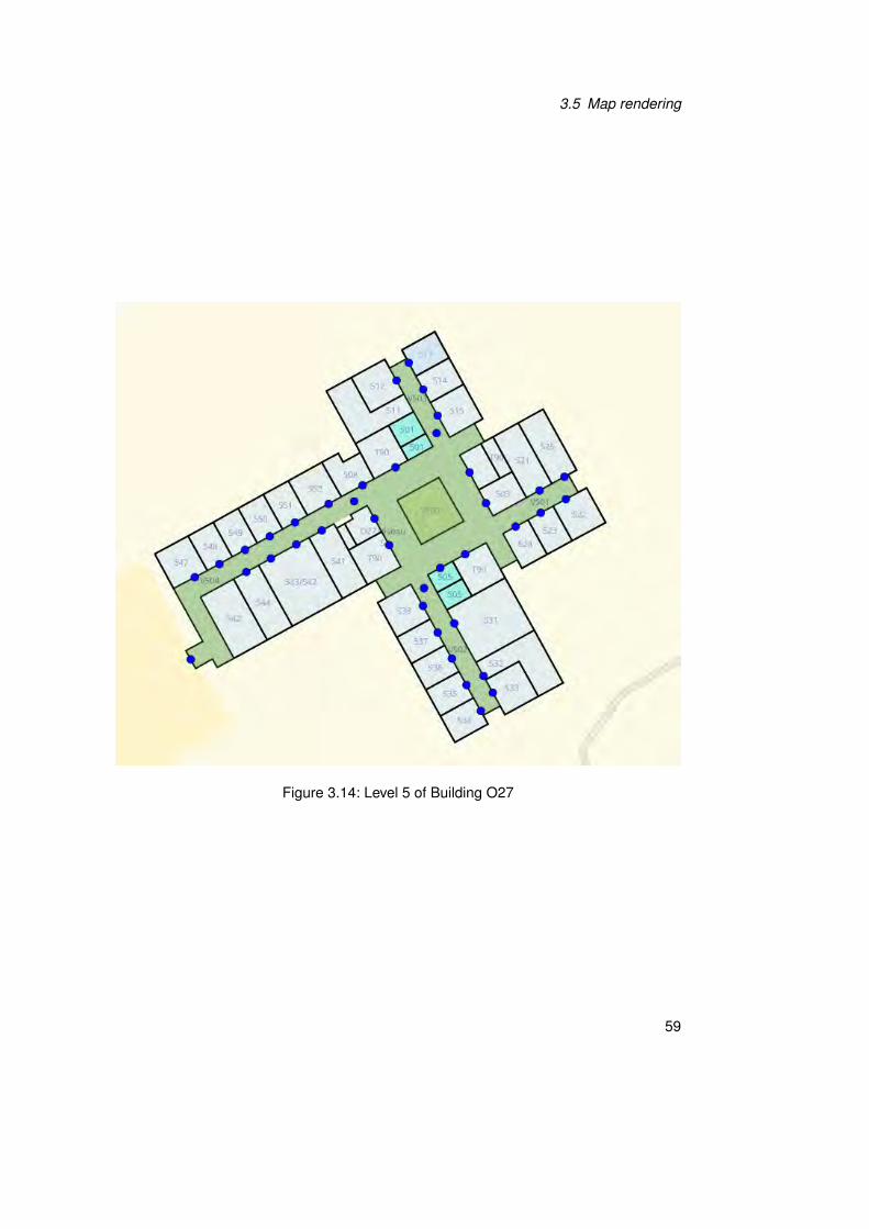
3.5 Map rendering
Figure 3.14: Level 5 of Building O27
59

3 Cartography on the University of Ulm Campus
tiles have to be created for every request. Because of the nature of an indoor mapping
environment, a higher zoom level is required compared to regular maps. Renderd does
not have a configuration option to specify a higher zoom level, the maximum zoom level is
only a compile time option. Listing D.3 is a patch for the render_config.h file, to enable a
zoom level of 22. The default configuration allows a maximum zoom level of 18, which is
not high enough for an indoor map.
The configuration for renderd is used to configure the rendering system as well as the
endpoints for map tile requests. Every building level needs its own endpoint as well as
its own Mapnik XML schema. The URLs used for the map server are osm_level<level
number>/, in the case of the test server with the hostname example.org, the full URL
for map tiles from building Level 1 would be: http://example.org/osm_level1. The full
configuration file is available in Listing D.4.
Conclusion
The documentation in this chapter does not cover all objects that may be encountered on
the campus as a whole. As such the documentation will evolve further as more parts of
the university are added. Some buildings will feature items, that need to be tagged and
were simply not encountered during the mapping process of this building.
The next chapter describes, how the data created using the information and processes
from this chapter, can be used to perform routing, displaying a map, and provide a
database of point-of-interest information.
60

4 Implementation
This chapter covers the implementation of the server side components not directly related
to mapping, as well as the client side application, in the form of an Android application.
The code name for the application is WiFinder and the application as well as the web
service carry this name.
Requirements
The following requirements exist on the server side:
• Server side hosting of Wi-Fi positioning system calibration data
• Server side computation of a users current position based on a scan of Wi-Fi signal
strengths
• Calculation of a route between two rooms
• Calculation of a route between the users current location and a room
• A database of the position of all rooms
• Ability to query the position of a room
To fulfill this criteria, a RESTful web service [17] was implemented using the Python
programming language [19].
The following requirements exist on the client side:
• Provide the user with an estimate of his current position including his current level
• Display the users position on a map view
61

4 Implementation
• User interface to show a route between two rooms
• User interface to show a route from the users current location to another room.
4.1 Overview
To get a better understanding of the implementation, Figure 4.1 shows an overview of the
components and their connection within the implementation.
ServerAndroid Smartphone
Rendering-Database
POI & WiFi fingerprint database
Wi-Fi AP
Wi-Fi AP
Wi-Fi AP
Rendering service
Web service
Figure 4.1: Overview of the infrastructure
The components fulfill the following purpose:
• Web service with a RESTful API
◦ Route calculation
◦ Wi-Fi fingerprint database
◦ Calculation of smartphone position
◦ Resources to access position of rooms
62

4.2 Design choices
• Two PostGIS databases
1. Database used to render the map
2. Database for Wi-Fi fingerprints and map POIs
• Android application
◦ Capture Wi-Fi fingerprints (offline phase)
◦ Display Map
◦ User interface for route calculation
4.2 Design choices
Considering the nature of this prototypical implementation, no caching of the information
received from the web service is performed. In a later implementation that is meant for
public consumption, caching should be implemented to reduce the server load as well as
decrease the response time of the application. The server oriented architecture eliminates
the problems of keeping the data in sync between the device and the server, and simplifies
the maintenance of the code related to routing and positioning, since only the server side
software needs to be changed.
4.3 Web service
The web services based on the RESTful architectures style was implemented. The
implementation was done using a Python framework called Flask [54] in combination with
a number of other Python modules, noteworthy being:
sqlalchemy A Python SQL Toolkit and Object Relational Mapper used for all database
access [57]
63

4 Implementation
geoalchemy2 An extension of sqlalchemy for working with geospatial databases [22]
Flask
The implementation of the service was done using the flask microframework for Python.
Flask simplifies the task of creating a web service while also giving the developer full
control over all aspects of the application. Flask allows the developer control over all
aspects of the application, while providing sensible defaults for these options.
RESTful Webservice
The API to provide all the features relies on the RESTful pattern along with JSON [13] as
serialization format. The API developed provides the following endpoints:
4.4 Positioning system
The positioning system is implemented using the principle of Wi-Fi fingerprinting, also
known as scene analysis. The explanation of how this system works is shown Section
2.4.
The system requires an offline and an online phase, where the offline phase is used to
create a database of fingerprints. The online phase consists of devices trying to determine
their location using the database.
The system works by using the map created from the campus in combination with an
Android device. The requirement for the hardware of the android device is an internet
connection as well as Wi-Fi module.
The software used for the offline as well as the online phase is the Wi-Finder Android
application which was developed in this thesis.
64

4.4 Positioning system
URL Method Data Type Description/entries GET HTML HTML view of all POI nodes in
the database/poi GET JSON Request a JSON repre-
sentation of a POI usingname=<NAME> argument. Ifno name is given, all POIs arereturned
/poi/names GET JSON Get a list of all names in thedatabase
/signalNodes/GET JSON Retrieve all SignaNodes from
the databasePOST JSON Submit a new SignalNode to
the database/signalNodes/<id:int> GET JSON Retrieve the SignalNode with
the given id
/getLocationGET JSON List of Wi-Fi Signal scans,
equivalent to SignalNodesPOST JSON Returns the users approximate
location given a signal scan/route GET JSON Needs a start and end URL
parameter, calculates a routebetween two points, and returnsthe route as a JSON list of way-points
/nav POST JSON Calculates a route based on thelocation given in the POST re-quest to the room given as astart URL argument
Table 4.1: Endpoints provided by the Wi-Finder API [59]
65

4 Implementation
4.4.1 Data storage
The storage of the information from the positioning system is done using the web service’s
database. The data in the database consists of the data created using the fingerprinting
system for positioning information as well as OpenStreetMap data. The OpenStreetMap
data is based on the same raw data that is used for the map rendering system, but has to
be held in two separate databases because of the differences in how the data is stored in
the database.
Data for the rendering server is uploaded using the osm2pgsql tool while data for the
POI service is created using the osmosis tool. The databases are separate, because
OSM tags are stored using the key/value system provided through Postgresql’s HSTORE
functions. The rendering toolchain does not work with the HSTORE system.
Osmosis
Osmosis is a command-line utility in principle similar to osm2pgsql but with the ability to
perform larger and more configurable operations [67]. The data that is uploaded to the
database is the same raw data that is used to create the rendering database, but osmosis
expects a cleaner format than osm2pgsql. All data (nodes, ways, relations) that is
uploaded using osmosis need version information as well as timestamps. JOSM does not
export OSM XML data with this information. To overcome this problem, an XML parser
written in Python is used to add the missing information using dummy values. The source
code for this parser is shown in Listing D.7. To automate the process of conversion and
upload a small bash script is used, as shown in Listing D.8.
A fingerprint taken for the positioning system contains the following information:
• The position of the smartphone. This location is defined by the user performing the
scan. The scan consists of latitude, longitude, and the building level.
• Signal strength of all Wi-Fi access points in range. The data captures for each signal
includes:
◦ Signal strength in dBm
66

4.4 Positioning system
◦ Frequency of the signal
◦ SSID of the access point
◦ MAC address of the access point
• The model of the smartphone
• A time stamp added by the web service when the node is uploaded
The data is transmitted from the smartphone using the JavaScript Object Notation (JSON)
and saved in the database. Using the API, a JSON representation of a SignalNode can be
retrieved. Listing 4.1 is an example of such a SignalNode, shortened to only two signals.
The full representation of this node with the id 12 would have had 16 signals.
Listing 4.1: A shortened example of a Signal Node
1 {
2 "signalNodes": {
3 "level": 2,
4 "timestamp": "2013-04-03 15:05:49",
5 "longitude": 9.95694693177938,
6 "signals": [
7 {
8 "ap": {
9 "ssid": "eduroam",
10 "bssid": "00:1e:4a:54:f6:f0"
11 },
12 "signal_strength": -56,
13 "frequency": 2412,
14 "id": 157
15 },
16 {
17 "ap": {
18 "ssid": "eduroam",
19 "bssid": "00:1e:4a:57:76:a0"
67

4 Implementation
20 },
21 "signal_strength": -80,
22 "frequency": 5280,
23 "id": 158
24 },
25 ],
26 "device": "GT-I9100",
27 "latitude": 48.4231721291727,
28 "id": 12
29 }
30 }
The storage in the database is done using three tables with relationships between them.
Figure 4.2 shows the schema and the relations between the tables in detail.
SignalNode
SignalStrength
AccessPoint
id intPK
level int
tstamp DateTime
latitude Float
longitude Float
device String
id intPK
signal_strength int
ap_bssid String
node_id int
frequency int
bssid StringPK
ssid String
Figure 4.2: Wi-Fi fingerprints database schema
68

4.4 Positioning system
Parameter Value DescriptionTP1 −85 Minimal signal strength in dBm an access point needs to be
used in the positioning algorithmTP3 −70 If signal strength of an access point is > TP3 and the signal
node is not in the calibration node, the calibration node is notused
apThreshold 3 If less than apThreshold APs match between the positioningscan and calibration node, calibration node is not used
neighbors 5 Number of SignalNodes at most averaged into the location
Table 4.2: Parameters in use for the positioning algorithm
4.4.2 Positioning algorithm
The algorithm used for the positioning system is based on the principle of Wi-Fi finger-
printing in combination with an euclidean distance based algorithm to determine the
position. The algorithm used in the implementation is an implementation of Dijkstra’s
algorithm as described in Section 2.3.1. The algorithm adds the component of averaging
the distance between the fingerprints, known as SignalNodes in the implementation.
Algorithm 2 is the first part of the process of calculating a position. The Euclidean distance
is calculated to all SignalNodes that match the criteria as stated in Section 2.5.3. The
implementation uses the parameters from Table 4.2 for the algorithm. The values are
based on the work in [21] but were changed based on experimentation using the developed
application.
The next step in the calculation of the position is the averaging of the weights which is
shown in Algorithm 3. The resulting level, latitude and longitude are the best possible
estimate of the users position.
69

4 Implementation
Algorithm 2 Part one of positioning algorithm in pseudo codeP is the position scan,D is the databasefor signal ∈ P do
if signal > TP1 thenmPosScan = mPosScan.append(signal)
end ifend forfor AP in mPosScan doquery = all SignalNodes in D which include AP
end forfor signalNode in query do
ap_counter = 0distance_vector = 0for positionSignal in mPosScan doexists = True {Check if BS with signal_strength > TP3 exists in this calibrationN-ode}if positionSignal[’signal_strength’] > TP3 then
exists = Falsefor calibrationSignal in calibrationNode.signals do
if calibrationSignal.ap_bssid == positionSignal[’ap’][’bssid’] thenexists = True
end ifend for
end ifif not exists then
break {Signal strength is larger than TP3, calibration node is not used for locating}else
for calibrationSignal in calibrationNode.signals doif positionSignal[′ap′][′bssid′] == calibrationSignal.apbssid thenap_counter = ap_counter + 1distance = calibrationSignal.signal_strength −positionSignal[′signal_strength′]distance = distance2
distance_vector = distance+ distance_vectorend ifELSE:continue {no breaks encountered}
end forend ifElse:if ap_counter > apThreshold theneuclidian_distance =
√distance_vectorap_counter
tuple = euclidian_distance, callibrationNodeadd tuple to positionListcontinue
end ifend for
end for
70

4.4 Positioning system
Algorithm 3 Part two of positioning algorithm in pseudo codeRequire: tuples of distance and signalNodes (positionList)
sort positionList from smallest to largest distance dindex, latitude, longitude, distances, level = 0for signalNode, distance in positionList do
if index < neighbors thenindex = index+ 1distances = (1/distances) + distanceslatitude = (node.latitude/distance) + latitudelongitude = (node.longitude/distance) + longitudelevel = (node.level/distance) + level
end ifend forlatitude = latitude/distanceslongitude = longitude/distanceslevel = level/distances
The position estimate is returned to the client using a JSON representation of the location,
an example of which can be seen in Listing 4.2
Listing 4.2: Example of a position as returned by the web service
1 {
2 "latitude": 48.4231721291727,
3 "longitude": 9.95694693177938,
4 "level": 2
5 }
4.4.3 Accuracy
To determine the accuracy of the positioning system a test series was done on two levels
of the building. On Level two the average deviation from the actual position was 3.84
meters. On Level three it was 6.76 meters. A total of 46 measurements were taken, five of
these measurements returned the wrong building level compared to the actual location.
The full test series is shown in Chapter B The accuracy that can be achieved varies
throughout the building. Factors like open spaces can contribute larger error margins. The
largest errors occur in stairways, where radio waves can travel mostly uninhibited between
71

4 Implementation
levels. As shown in the test series, the margin of error can be large enough such that the
position is off by a building level.
4.5 Routing
The RESTful web service is also responsible for the calculation of routes between rooms
or routes from the user’s location to a room. Navigation to an arbitrary point on the map is
not possible. The implementation of the routing algorithm uses the endpoints of the web
service as defined in Table 4.1. The actual implementation is based on Dijkstra’s algorithm,
which is explained in detail in Section 2.3.1. The full source code of the implementation is
shown in Listing D.6.
4.5.1 Implementation of a Dijkstra algorithm
To be able to calculate a route using a shortest path algorithm, a graph is needed. The
graph is constructed using elements from the OpenStreetMap project. The graph is
constructed with the JOSM in the form of ways with the tag highway=corridor. Because of
how the routing algorithm works, all the nodes on theses ways need to be tagged with
a level tag. These paths are later used to construct the waypoints that are used for the
route. The process of constructing this graph consists of connecting all nodes that are
tagged with the entrance = yes with the ways. Since the ways are used for the routing
process, the path that these ways take in the corridors must not be obstructed by walls or
other obstacles. Figure 4.3 shows the ways that were constructed in building Level 1.
72

4.5 Routing
Figure 4.3: Routing paths of Building O27, Level one
4.5.2 Getting a route
The web service needs two parameters to be able to construct the route: a room number
where the route starts and a room number where the route ends. These are transmitted in
the URL of the request that is transmitted to the web service using URL parameters, for ex-
ample http://example.org/poi-service/route/?start=O27%20245&end=H20
represents the route from the office in room O27 245 to the auditorium H20.
The web service returns a list of waypoints to the client questing a route, an example of
which is shown in Listing 4.3.
Listing 4.3: Example of a route from room O27 245 to O27 201
1 {
2 "waypoints": [
73

4 Implementation
3 {
4 "latitude": 48.42282045409622,
5 "longitude": 9.956953558398476,
6 "level": "2"
7 },
8 {
9 "latitude": 48.422857374806135,
10 "longitude": 9.957059467154115,
11 "level": "2"
12 },
13 {
14 "latitude": 48.42282647162592,
15 "longitude": 9.957096769402563,
16 "level": "2"
17 },
18 {
19 "latitude": 48.422840172020194,
20 "longitude": 9.95714660380187,
21 "level": "2"
22 },
23 {
24 "latitude": 48.42284657089658,
25 "longitude": 9.957166790861855,
26 "level": "2"
27 },
28 {
29 "latitude": 48.42283814387136,
30 "longitude": 9.957175493101834,
31 "level": "2"
32 }
33 ]
34 }
74

4.6 Android application
Since the data type being returned is a list, no numbering of waypoints is required. The
order is defined by the data type and as such by the order in which the items are returned.
The data format is held as simple as possible and makes the usage through any other
type of application which wants to perform routing functions inside the campus possible.
This makes way for future projects that need a routing API on the campus. By drawing a
line from the starting waypoint to the last item in the list, a route can be constructed.
4.5.3 Routing from the users current location
The second aspect of routing is using the information from the positioning system in
combination with the routing system. The user transmits his current location to the web
service using the endpoint nav. The web service computes a route using the same
algorithms that are used when routing between two rooms. But because the starting point
is usually not an already defined point, the process is more complex.
The routing process works by finding the point on the navigation grid as defined in Figure
4.3 that is closest to the starting point of the routing process. The process works by using
PostGIS functions to determine the nearest neighbor that matches the characteristics
of the routing grid nodes. Once such a point is determined, the routing process works
exactly the same as routing between two rooms. The route is returned in the same JSON
format as seen in Listing 4.3.
4.6 Android application
The component a user interacts with directly is a smartphone application developed for
the Android platform.
4.6.1 Choosing a platform
In the planning stages of the project, the three largest smartphone platforms were consid-
ered for the development of the end user component. The results of other papers were
75

4 Implementation
also taken into consideration during the process of choosing the implementation platform
[49], [53], and [55]. These platforms are:
• Apple’s iOS [28]
• Microsoft’s Windows Phone 7 [43]
• Google’s Android [30]
The deciding factor for the choice of the platform was the possibility to access the devices
information about Wi-Fi access points in range and their signal strength. Only the Android
platform has an interface in it’s SDK which allows access to this information. Windows
Phone and iOS only provide information about the connected networks or the network
state, Windows Phone provides information about the SSID of the connected network
[44], but not the signal strength or the MAC addresses [7] of the access points in range.
As a result of this required feature, only the Android platform could be used to implement
the positioning system as envisioned in the planning stages.
4.6.2 Android implementation
The Android implementation is built to be backwards compatible up to Android version
2.0. This backwards compatibility is needed because of the fragmentation of the Android
smartphone market. The most prevalent version of Android is 2.3 with a market share
of 36.4%. Building an application that is only compatible with versions starting from 4.0
would, at the time this application was developed, only work on 58.6% of devices. The full
set of statistics that show the grade of fragmentation can be seen in Table 4.3.
4.6.3 Libraries
The following libraries are used for the Android application:
ActionBarSherlock A backport of the Android action bar pattern and fragments. The
action bar is used to provide a standardized navigation interface for android applica-
76

4.6 Android application
Version Codename API Distribution1.6 Donut 4 0.1%2.1 Eclair 7 1.5%2.2 Froyo 8 3.2%2.3 - 2.3.2 Gingerbread 9 0.1%2.3.3 - 2.3.7 Gingerbread 10 36.4%3.2 Honeycomb 13 0.1%4.0.3 - 4.0.4 Ice Cream Sandwich 15 25.6%4.1.x Jelly Bean 16 29.0%4.2.x Jelly Bean 17 4.0%
Table 4.3: Android fragmentation on June 3, 2013 [31]
tions, but was only added with the Android API 13. ActionBarSherlock allows the
usage of this pattern with Android versions 2.x and up [3]. Another feature provided
by ActionBarSherlock is its own implementation of the Android fragment pattern
Google Play Services The Google play services library provides the Google Map View
that is used to display the map tiles from the rendering server [25]. The Google Play
Services SDK provides this in the form of the “Google Maps Android API v2” [33].
Gson or “Google-Gson” “ is a Java library that can be used to convert Java Objects
into their JSON representation. It can also be used to convert a JSON string to an
equivalent Java object.” [23]. The library is used to convert the data from the web
service to Java objects.
4.6.4 Android implementation details
The Android implementation uses elements as suggested by the Android API guides when
possible. The user interface is constructed using the action bar pattern for navigation and
fragments to construct the individual views.
ActionBar
The action bar is a window on the upper edge of an application that provides a dedicated
space for navigation purposes. Through the use of the action bar, a consistent navigation
view can be provided across as many android applications as possible [2].
77

4 Implementation
Figure 4.4: Action bar as used in the Wi-Finder application
The action bar as used in the Wi-Finder application is shown in Figure 4.4, the action
bar provides three tabs to switch between the different views of the application. In the
example shown, the action bar also provides three buttons to access features of the view
currently being displayed as well as the so called “overflow” menu, accessed using the “... ”
symbol.
The items shown in the action bar depend on the amount of screen real estate available
on the device. The items that cannot be shown on screen are moved to the menu button,
that is accessed using the menu key of the device.
Fragments
Fragments are components that hold the views being displayed. Fragments are primarily
designed to “support more dynamic and flexible UI designs on large screens, such as
tablets” [20]. The fragments implementation used in the application is the backported
fragment from the ActionBarSherlock library.
4.6.5 Application views
This section provides a description of what features are provided by each of the available
views and how these views are implemented.
The application has the following main views:
AP List A small view which displays a list of Wi-Fi access points currently in range along
with metadata for every access point.
78

4.6 Android application
Figure 4.5: Smartphone screen of the Wifinder map view
79

4 Implementation
Item Description
Start the positioning system
Switch the map view to a different building level
Open the dialog to get directions
Open the preferences screen
Table 4.4: Menu items in the map view
Map This is the default map view. It shows a map of the campus and provides features
for locating the user as well as the routing functionality
Wi-Fi Map This map view is used to perform the fingerprinting phase of the Wi-Fi posi-
tioning system.
Map
The most important view in the application is the map view. Figure 4.5 shows how this
view looks on a smartphone and Figure 4.6 shows the same view on an Android tablet.
The map view combines all the information from the mapping process by displaying the
map tiles as rendered by the server and can enable the positioning system. The menu
items offered in this view along with a description of their functions can be seen in Table
4.4.
The view includes a widget to switch between building levels in the form of a menu item
“BUILDING LEVEL”, the menu of which is shown in Figure 4.7.
Positioning system
The implementation consists of a specially crafted SherlockMapFragment based on Go-
ogle’s Android Map API v2 and components of the ActionBarSherlock library. To display
the map a MapTools class is used as a helper. It tailors the map view depending on
80

4.6 Android application
Figure 4.6: Screenshot of the map view of Level 1, Building O27
81

4 Implementation
Figure 4.7: Widget to switch between building levels
82

4.6 Android application
the required information and instantiates the maps canvas. It handles the display of a
route and any other functions that need to draw items on the map. The Locate Me button
starts the applications positioning system. It starts a service that is called when new
position information is available. The specifics of this service are explained in detail later
in this chapter. A marker is shown on the map once a position has been determined. This
marker is shown in Figure 4.8 along with a pop up showing detailed information about the
acquired position. Once a new location is determined, the marker is updated to reflect this
change.
If the marker is not visible on the current map canvas, the canvas is updated so that the
marker is centered on the screen. The map also changes the building level shown, based
on the calculated position.
Routing
The map view includes the functionality required to query the web service for routes and
display the returned route on the maps canvas. The calculated route is then displayed on
the map canvas, so that a person can follow the path and reach their destination. To get
the directions the user opens the Get Directions dialog enters a start and an end point of
his route, as shown in Figure 4.9. The text fields need the unique identifiers of the rooms
as set in Section 3.4.3. The text fields uses auto completion to show suggestions in a drop
down list below the text box during text input (Figure 4.10). This simplifies the data entry
process for the user, since all possible values are part of the auto complete function. The
auto complete function is implemented by querying the web service for a list of all rooms.
Besides the possibility to specify a starting and a end room, a check box can be used to
specify that the current location should be used as the starting point of the route.
83

4 Implementation
Figure 4.8: Marker showing the devices calculated position
84

4.6 Android application
Figure 4.9: Dialog to request directions between two rooms
85

4 Implementation
Figure 4.10: Auto completion function of the Get Directions dialog
86

4.6 Android application
Figure 4.11: Example of a route as displayed on the canvas
87

4 Implementation
Item Description
Record a Wi-Fi fingerprint at the position indicatedand send it to the web service
Switch the map view to a different building level
Open the preferences window
Table 4.5: Menu items in the Wi-Fi Map screen
Once the user has entered the required information and has clicked the Get Directions
button, the route is calculated using the web services API and the result is then shown in
the map canvas in the form of a blue line from the starting point to the end point. Figure
4.11 is an example of a route as it is displayed on the map’s canvas.
WiFi Map
The WiFi Map uses the same tools to construct a map canvas as the Map screen, but
serves an entirely different purpose. It can be seen as the development front end of the
Wi-Fi positioning system. The map displayed is the same canvas as the Map view, but
with some added features to help with the process of capturing Wi-Fi fingerprints. The
first thing a users sees is that the canvas is overlayed with a grid with a mesh size of five
meters. The grid is shown to have frame of reference when creating Wi-Fi fingerprints.
Without such a grid it is not immediately apparent where fingerprints need to be placed.
Another visible feature in this view are markers on the map. Each marker represents an
existing Wi-Fi fingerprint. The Wi-Fi fingerprints are downloaded from the API service
when the map view is loaded, so that the view always shows an up to date view of the
fingerprints.
The view of the existing fingerprints makes it easier for a user to add missing fingerprints,
since he can see where fingerprints were already taken. Another feature provided by the
markers is the ability to delete fingerprints. This is useful, if a fingerprint was taken at
the wrong location or fingerprints need to be updated. Because the device can provide
88

4.6 Android application
the needed functionality to change the fingerprints in the database, no other software is
required to manage the fingerprints.
Fingerprinting
The main purpose of this view is to take fingerprints for the Wi-Fi positioning system. The
process consists of the following steps:
1. The application on the device is started and the Wi-Fi fingerprint view is loaded.
2. The user selects the level he wants to take fingerprints on.
3. The user walks to the position where he wants to take the fingerprint at.
4. On the applications map canvas, the blue crosshairs are moved to the position the
user is currently at, as seen in Figure 4.14.
5. The user presses the SEND WIFI FINGERPRINT button.
6. The dialog in Figure 4.15 is displayed. during the fingerprinting process. During
this phase, the applications service queries the Wi-Fi radio and receives a callback
when the results are available. Then the fingerprint is uploaded to the web service,
where the fingerprint is stored in the database. Once this process is complete, the
dialog is closed. The user must not move during this process, since otherwise the
fingerprint will not be at the users current location.
7. A marker is shown on the map canvas at the location the fingerprint was created.
The process of deleting a fingerprint involves clicking that fingerprints marker. The dialog
in Figure 4.15 is shown and once the user confirms the deletion, the fingerprint is deleted
using the web service.
AP List
The AP list view was originally conceived as a test bed for parts of the application like the
background service that queries the Wi-Fi module for access points. It has remained in
89

4 Implementation
Figure 4.12: Mesh grid and existing fingerprints in the Wifi Map screen
90

4.6 Android application
Figure 4.13: Dialog asking for confirmation that a Wi-Fi fingerprinting node is to be deleted
91

4 Implementation
Figure 4.14: Crosshairs used to show the position of the fingerprint
92

4.6 Android application
Figure 4.15: Dialog shown when a fingerprint is taken
the application since it is a valuable tool to check the Wi-Fi reception and the number of
access points currently in range. It’s functionality consists of querying the Wi-Fi service for
access points and displaying them in a ListFragment, a fragment designed to display a list
of items. An example of this view is shown in Figure 4.16, To get more information about
an access point, it can be clicked. The information consists of all information available
about the given access point, including signal strength and capabilities. Figure 4.17 is an
example of the detailed view.
Figure 4.16: A list of access points in the AP List scanner view
93

4 Implementation
Figure 4.17: Detailed view of an access point in the AP list view
Preferences
Wifinder Preferences
Wi-Fi Fingerprinting
Draw grid over map
Server URLs
Tileserver for indoor map tiles
POI Service URL
Figure 4.18: Structure of preferences
94

4.6 Android application
The application also features a preferences screen, where some settings can be influenced.
The settings are mostly related to server URLs, since these were sometimes changed to
reflect the usage of the debugging servers during the development phase. The preferences
are split into two different preference screens, the Wi-Fi Fingerprinting preferences as
well as the Server URLs preferences screen. The preferences can be accesses in any
part of the application using the devices Menu button when available. The structure of the
preferences can be seen in Figure 4.18. Figure 4.19 shows the actual preferences window
in the application. The implementation is done using Android’s preference management
API [6].
Figure 4.19: Preferences screen of the application
Server preferences
The preferences in this part allow the user to change the URL opened for the map tiles as
well as the URL used for the calls to the web services. The URLs can be changed using a
text field, when the corresponding entry is clicked in the preferences screen.
95

4 Implementation
Fingerprinting preferences
The fingerprinting preferences are used to enable or disable the mesh grid that is shown
on the Wi-FiMap canvas.
Wi-Fi service
The implementation of the Wi-Fi service is responsible for the querying of the device’s Wi-
Fi radio and providing applications with the results. The system works through the usage
of Androids concept of System Services. These service send broadcasts to registered
receivers. A service can have a multiple broadcasts a receiver can subscribe to. In
the case of the applications Wi-Fi receiver, the system service WIFI_SERVICE and its
callback for new scan results is used. As an example of this usage, should a Wi-Fi
fingerprint be created, a BroadcastReceiver is created and registered. Then the
WIFI_SERVICE is instructed to scan for Wi-Fi signals and once this scan is complete, a
callback interface is used to notify the application that new results are available.
Network tasks
The Android application relies heavily on calls to the web service and rendering server to
perform its tasks. Without a network connection, the app has no functionality to speak of.
The specifics of this design choices are in Section 4.2. All calls to the web services are
handled in the background, which prevents the UI thread from freezing for the duration of
these requests. The Android SDK provides a class called AsyncTask, which can handle
these kind of background tasks.
“AsyncTask is designed to be a helper class around Thread and Handler and
does not constitute a generic threading framework. AsyncTasks should ideally
be used for short operations (a few seconds at the most.) If you need to keep
threads running for long periods of time, it is highly recommended you use the
various APIs provided by the java.util.concurrent pacakge such as Executor,
ThreadPoolExecutor and FutureTask.” [8]
96

4.6 Android application
The implementation uses these AsyncTasks to perform the background requests to the
web service and callbacks are used to inform the UI of the finished request, so that the UI
can update its screen as needed.
97


5 Outlook
The implementation in this work has succeeded in providing a system that can position a
user on the campus of the university, display a map of the interior of the building with a high
level of detail and provide directions to rooms in the building. The accuracy is high enough
for a user to be able to find his position on the map and have a better understanding of his
or her surroundings.
Requirements revisited
The following requirements for the client side were documented before the implementation
phase of the project:
1. Provide the user with an estimate of his current position including his current level.
2. Display the users position on a map view.
3. User interface to calculate a route between two rooms.
4. User interface to calculate a route from the users current location to another room.
Table 5.1 shows a listing of these requirements and their corresponding solution. Using
the implementation in this thesis, all requirements that were stated could be achieved. As
such the implementation is successful in providing a mapping system for the Building O27
with the potential to expand the coverage across the whole campus.
99

5 Outlook
Requirement Fulfillment1 The positioning system created can provide the user with a position
such that the user can see an estimate of his position inside the building.The position is not 100% accurate, but provides a best-effort solutionto this requirement.
2 The map canvas in the Android application can use the data from thepositioning system and show this position on the map.
3 A user interface to enter two rooms was implemented and the resultingroute is shown by the Android application.
Table 5.1: Requirements and their fulfillment
5.1 Challenges
One of the challenges of this system was the creation of high quality mapping material.
The process as outlined is highly manual and labor-intensive. The task of creating rooms
and manually tagging them is also error-prone. Considering the size of for example, the
campus of a university, the chances are high, that the maps will have errors. This can
lead to maps that do not correctly portray the location of rooms or show areas that do not
actually exist. These problems are not as serious as errors in the routing ways that are
computed inside buildings. Errors in this grid of paths can lead to longer routes, errors in
the routing algorithm, or rooms that can not be reached through navigation.
There are ways to reduce these errors. For example, an algorithm could be designed
that checks the reachability of all POIs in the web service and reports such errors before
new data is added to the database. Similar checks can be developed for other map
data, which check if rooms have inconsistent tags. Both of these can eliminate errors.
But these algorithms cannot decrease the amount of time needed to generate the map
material. A way that has been devised during this thesis, but could not be tested because
of time constraints, would be the automatic creation of map data from already existing
schematics. Such data is usually available for buildings in the form of AutoCAD [29] or
similar computer-aided-design software.
If a parser can be written that is able to produce map data for OSM, it can reduce errors in
the material and either decrease the amount of time needed to create maps or, in the best
case, automate the process as a whole. This would leave the Wi-Fi positioning system as
100

5.2 Future work
the last task that required a large amount of manual labor. But the advances in robotics
might be able to automate even this process.
5.2 Future work
The way the application is designed is very modular as the system used for Wi-Fi posi-
tioning is separate from the components used to render the map. The POI service and
Wi-Fi positioning both run on the same server, but can easily be separated from each
other, since there are no interdependencies. the usage of OSM tools brings a framework
of other software that can work with the created material. Through the usage of readily
available components that work with OSM data, other systems can profit from this data.
One such example is the OpenStreetMap project called “Slippy Map” [68]. It provides a
browser interface to map tiles. This interface was used to create a browser based map
of O27, using the OSM material created for this thesis. This application can be seen in
Figure 5.1. Such a map can be used throughout web sites of the campus to show the
location of rooms or events.
Positioning system
The accuracy of the positioning system can be improved to increase its accuracy. Table
2.3 shows that accuracies in the range of two meters are possible using Wi-Fi based
systems. Increasing the number of fingerprints is one way to increase the accuracy
of these positioning systems. Another way to increase the accuracy is by taking four
measurements at each fingerprint, in four different directions. This is used to reduce the
impact on the received signals strengths caused by the person performing this scan.
Routing
The routing system currently uses Dijkstra’s algorithm to find the shortest path between
two points. Using different algorithms, for example A*, can decrease the time needed to
calculate a route. Route calculation could also be performed on the device to decrease
the reliance on a internet connection. Especially, a visitor might not always have the
101

5 Outlook
Figure 5.1: OSM Slippy Map of building O27
102

5.3 Conclusion
needed credentials to use the University’s Wi-Fi system or even know of it’s existence. The
reception from the cell phone network is not always reliable and especially in underground
levels unreliable at best. Another possibility is the optimization of routes in the context of
process management and mobile process management, examples that can profit from
this work are [51] and [50].
App enhancements The functionality of the app can also be expanded to include more
meta information. One idea that can be envisioned using the map material in combination
with other data could be an extension of the map, where clicking on a office can show the
occupants with phone numbers and other contact information. Clicking on an auditorium
could show information about the usage for the current day and the maximum occupancy.
Another possibility is the combination of the POI data with an augmented reality application.
This app could show the location of all rooms or the location of some of the more important
places on campus.
5.3 Conclusion
While the application leaves room for future enhancements, the application shows that
using the technologies as described in this thesis provide a system that constitutes a full
solution for indoor navigation. The concepts described in this system are fully transferable
to almost any other indoor environment, especially considering the prevalence of Wi-Fi
networks in most indoor environments.
103


Bibliography
[1] private communication. Department V - Facility management, University of Ulm,
July 2, 2013.
[2] Action Bar | Android Developers. June 25, 2013. URL: http://developer.andr
oid.com/guide/topics/ui/actionbar.html.
[3] ActionBarSherlock - Home. June 25, 2013. URL: http://actionbarsherlock
.com/index.html.
[4] A.V. Aho, J.E. Hopcroft, and J.D. Ullman. Data structures and algorithms: Addison-
Wesley series in computer science and information processing. Addison-Wesley,
1983. ISBN: 9780201000238. URL: http://books.google.de/books?id=Ast
QAAAAMAAJ.
[5] K. Al Nuaimi and H. Kamel. “A survey of indoor positioning systems and algorithms”.
In: Innovations in Information Technology (IIT), 2011 International Conference on.
2011, pp. 185–190. DOI: 10.1109/INNOVATIONS.2011.5893813.
[6] android.preference | Android Developers. June 26, 2013. URL: http://develo
per.android.com/reference/android/preference/package-summary
.html.
[7] IEEE Standars Association. Standard Group MAC Addresses: A Tutorial Guide.
URL: http://standards.ieee.org/develop/regauth/tut/macgrp.pdf
(visited on 07/02/2013).
[8] AsyncTask | Android Developers. June 26, 2013. URL: http://developer.and
roid.com/reference/android/os/AsyncTask.html.
[9] Alexander Bachmeier. Indoor Ortung und Kartografie. Ulm University, 2013.
[10] Bing Maps. URL: http://www.bing.com/maps/ (visited on 07/01/2013).
[11] CartoCSS | MapBox. June 18, 2013. URL: http://www.mapbox.com/tilemil
l/docs/manual/carto/.
105

Bibliography
[12] Core Concepts of Mapnik — mapnik Wiki. June 18, 2013. URL: https://github
.com/mapnik/mapnik/wiki/MapnikCoreConcepts.
[13] D. Crockford. The application/json Media Type for JavaScript Object Notation (JSON).
RFC 4627 (Informational). Internet Engineering Task Force, July 2006. URL: http:
//www.ietf.org/rfc/rfc4627.txt.
[14] Zhang Da et al. “Localization Technologies for Indoor Human Tracking”. In: CoRR
abs/1003.1833 (2010). URL: http://dblp.uni-trier.de/db/journals/co
rr/corr1003.html#abs-1003-1833.
[15] E. W. Dijkstra. “A note on two problems in connexion with graphs”. In: Numerische
Mathematik 1.1 (Dec. 1, 1959), pp. 269–271. ISSN: 0029-599X. DOI: 10.1007/bf
01386390. URL: http://dx.doi.org/10.1007/bf01386390.
[16] FAQ — Mapnik. URL: http://mapnik.org/faq/.
[17] Roy Thomas Fielding. “Architectural styles and the design of network-based software
architectures”. AAI9980887. PhD thesis. University of California, Irvine, 2000. ISBN:
0-599-87118-0.
[18] Kenneth E. Foote and University of Texas at Austin) Lynch, Margaret (Department
of Geography. Principles of Geographical Information Systems. 2000. URL: http:
//www.rc.unesp.br/igce/geologia/GAA01048/papers/Burrough\_Mc
Donnell-Two.pdf (visited on 05/23/2013).
[19] Python Software Foundation. Python Programming Language - Official Website.
URL: http://www.python.org/ (visited on 07/02/2013).
[20] Fragments | Android Developers. June 25, 2013. URL: http://developer.and
roid.com/guide/components/fragments.html.
[21] S. Gansemer, U. Grossmann, and S. Hakobyan. “RSSI-based Euclidean Distance
algorithm for indoor positioning adapted for the use in dynamically changing WLAN
environments and multi-level buildings”. In: Indoor Positioning and Indoor Navigation
(IPIN), 2010 International Conference on. 2010, pp. 1–6. DOI: 10.1109/IPIN.20
10.5648247.
[22] Geoalchemy2 Documentation. June 20, 2013. URL: http://geoalchemy-2.re
adthedocs.org/en/0.2/.
[23] google-gson - A Java library to convert JSON to Java objects and vice-versa.
June 26, 2013. URL: https://code.google.com/p/google-gson/.
106

Bibliography
[24] Google Maps - University of Ulm Campus. June 11, 2013. URL: https://www.g
oogle.de/maps/preview#!data=!1m4!1m3!1d3206!2d9.9584841!3d48
.4236206.
[25] Google Play Services | Android Developers. June 25, 2013. URL: http://dev\-
eloper.android.com/google/play-services/index.html.
[26] P.E. Hart, N.J. Nilsson, and B. Raphael. “A Formal Basis for the Heuristic Deter-
mination of Minimum Cost Paths”. In: Systems Science and Cybernetics, IEEE
Transactions on 4.2 (1968), pp. 100–107. ISSN: 0536-1567. DOI: 10.1109/TSSC
.1968.300136.
[27] How MySQL Uses Indexes. Oracle Corporation. URL: http://dev.mysql.com
/doc/refman/5.1/en/mysql-indexes.html (visited on 05/25/2013).
[28] Apple Inc. Apple - iOS - 6. URL: http://www.apple.com/ios/ (visited on
07/02/2013).
[29] Autodesk Inc. AutoCAD Design Suite | CAD Design Software | Autodesk. Autodesk
Inc. 2013. URL: http://www.autodesk.com/suites/autocad-design-su
ite/overview (visited on 07/02/2013).
[30] Google Inc. Android. URL: http://www.android.com/ (visited on 07/02/2013).
[31] Google Inc. Dashboards | Android DEvelopers. June 25, 2013. URL: http://dev
eloper.android.com/about/dashboards/index.html.
[32] Google Inc. Google Maps. July 1, 2013. URL: https://www.google.com/maps.
[33] Google Inc. Google Maps Android API v2 – Google Developers. URL: https://
developers.google.com/maps/documentation/android/ (visited on
07/03/2013).
[34] Introduction | MapBox. June 18, 2013. URL: http://www.mapbox.com/tilemi
ll/docs/manual/.
[35] Javier DeSalas Jimmy LaMance and Jani Järvinen, eds. Innovation: Assisted GPS:
A Low-Infrastructure approach. GPS World (Mar. 1, 2002). URL: http://www.gp
sworld.com/innovation-assisted-gps-a-low-infrastructure-app
roach/ (visited on 06/27/2013).
[36] JOSM - OpenSteetMap Wiki. June 10, 2013. URL: http://wiki.openstreetm
ap.org/w/index.php?title=JOSM&oldid=908119.
107

Bibliography
[37] JOSM/Plugins - OpenStreetMap Wiki. June 10, 2013. URL: https://wiki.open
streetmap.org/w/index.php?title=JOSM/Plugins&oldid=802496.
[38] Josm/Plugins/PicLayer. June 13, 2013. URL: http://wiki.openstreetmap.o
rg/w/index.php?title=JOSM/Plugins/PicLayer&oldid=734413.
[39] mapbox/osm-bright - GitHub. June 18, 2013. URL: https://github.com/mapb
ox/osm-bright.
[40] Map Features - OpenSteetMap Wiki. June 10, 2013. URL: http://wiki.openst
reetmap.org/w/index.php?title=Map_Features&oldid=836071.
[41] MapQuest maps - Driving Directions - Map. URL: http://www.mapquest.com/
(visited on 07/01/2013).
[42] Brian McClendon. A new frontier for Google Maps: mapping the indoors. Nov. 29,
2011. URL: http://googleblog.blogspot.de/2011/11/new-frontier-
for-google-maps-mapping.html (visited on 06/29/2013).
[43] Microsoft. The Smartphone Reinvented Around You | Windows Phone (United
States). URL: http://www.windowsphone.com/en-us (visited on 07/02/2013).
[44] MSDN. NetworkInterfaceInfo.InterfaceName Property. May 2013. URL: http://m
sdn.microsoft.com/en-us/library/windowsphone/develop/microso
ft.phone.net.networkinformation.networkinterfaceinfo.interfa
cename(v=vs.105).aspx.
[45] NAVSTAR GPS USER EQUIPMENT INTRODUCTION. 1996. URL: http://www
.navcen.uscg.gov/pubs/gps/gpsuser/gpsuser.pdf.
[46] OpenGeo : Introduction to PostGIS : Section 1: Introduction. 2013. URL: http://w
orkshops.opengeo.org/postgis-intro/introduction.html (visited on
05/24/2013).
[47] OpenSteetMap - Copyright and License. June 8, 2013. URL: http://www.opens
treetmap.org/copyright/en.
[48] OpenStreetMap project. OpenStreetMap. URL: http://www.openstreetmap.o
rg/ (visited on 07/01/2013).
[49] Rüdiger Pryss et al. “Mobile Task Management for Medical Ward Rounds - The
MEDo Approach”. In: 1st Int’l Workshop on Adaptive Case Management (ACM’12),
BPM’12 Workshops. LNBIP 132. Springer, Sept. 2012, pp. 43–54.
108

Bibliography
[50] Rüdiger Pryss et al. “Towards Flexible Process Support on Mobile Devices”. In:
Proc. CAiSE’10 Forum - Information Systems Evolution. LNBIP 72. Springer, 2010,
pp. 150–165.
[51] Manfred Reichert and Barbara Weber. Enabling Flexibility in Process-Aware Infor-
mation Systems: Challenges, Methods, Technologies. Berlin-Heidelberg: Springer,
2012.
[52] Relation - OpenSteetMap Wiki. June 8, 2013. URL: http://wiki.openstreetm
ap.org/w/index.php?title=Relation&oldid=876549.
[53] Andreas Robecke, Rüdiger Pryss, and Manfred Reichert. “DBIScholar: An iPhone
Application for Performing Citation Analyses”. In: CAiSE Forum-2011. Proceed-
ings of the CAiSE’11 Forum at the 23rd International Conference on Advanced
Information Systems Engineering Vol-73. CEUR Workshop Proceedings, June 2011.
[54] Armin Ronacher. Welcome | Flask (A Python Microframework). URL: http://fla
sk.pocoo.org/ (visited on 07/02/2013).
[55] Johannes Schobel et al. “Using Vital Sensors in Mobile Healthcare Business Ap-
plications: Challenges, Examples, Lessons Learned”. In: 9th Int’l Conference on
Web Information Systems and Technologies (WEBIST 2013), Special Session on
Business Apps. 2013 SCITEPRESS, May 2013, pp. 509–518.
[56] Uwe Schöning. Algorithmik. Spektrum Akadem. Verl., 2001, pp. 1–384. ISBN: 978-
3-8274-1092-4.
[57] SQLAlchemy - The DataData Toolkit for Python. June 20, 2013. URL: http://ww
w.sqlalchemy.org/.
[58] Tags - OpenStreetMap Wiki. June 9, 2013. URL: http://wiki.openstreetmap
.org/w/index.php?title=Tags&oldid=867416.
[59] OpenStreetMap Wiki. About — OpenStreetMap Wiki, [Online; accessed 8-June-
2013]. 2013. URL: http://wiki.openstreetmap.org/w/index.php?title
=About&oldid=905556.
[60] OpenStreetMap Wiki. Beginners Guide 1.3 — OpenStreetMap Wiki, [Online; ac-
cessed 8-June-2013]. 2013. URL: http://wiki.openstreetmap.org/w/ind
ex.php?title=Beginners_Guide_1.3&oldid=908918.
[61] OpenStreetMap Wiki. Bing — OpenStreetMap Wiki. June 17, 2013. URL: http://w
iki.openstreetmap.org/w/index.php?title=Bing&oldid=869138.
109

Bibliography
[62] OpenStreetMap Wiki. Elements — OpenStreetMap Wiki, June 8, 2013. URL: http:
//wiki.openstreetmap.org/w/index.php?title=Elements&oldid=89
5354.
[63] OpenStreetMap Wiki. History of OpenStreetMap — OpenStreetMap Wiki, [Online;
accessed 7-June-2013]. 2013. URL: http://wiki.openstreetmap.org/w/in
dex.php?title=History_of_OpenStreetMap&oldid=897370.
[64] OpenStreetMap Wiki. Mapnik — OpenStreetMap Wiki. June 16, 2013. URL: http:
//wiki.openstreetmap.org/w/index.php?title=Mapnik&oldid=9081
71.
[65] OpenStreetMap Wiki. Mod tile — OpenStreetMap Wiki. June 17, 2013. URL: http:
//wiki.openstreetmap.org/w/index.php?title=Mod_tile&oldid=90
4480.
[66] OpenStreetMap Wiki. Osm2pgsql — OpenStreetMap Wiki. June 17, 2013. URL:
http://wiki.openstreetmap.org/w/index.php?title=Osm2pgsql&ol
did=913771.
[67] OpenStreetMap Wiki. Osmosis - OpenStreetMap Wiki. June 25, 2013. URL: http:
//wiki.openstreetmap.org/w/index.php?title=Osmosis&oldid=888
510.
[68] OpenStreetMap Wiki. Slippy Map - OpenSteetMap Wiki. June 26, 2013. URL: http
://wiki.openstreetmap.org/w/index.php?title=Slippy_Map&oldid
=901993.
[69] Wikipedia. Cartography — Wikipedia, The Free Encyclopedia. [Online; accessed
7-June-2013]. 2013. URL: http://en.wikipedia.org/w/index.php?title
=Cartography&oldid=552817872.
[70] Wikipedia. Graph theory — Wikipedia, The Free Encyclopedia. [Online; accessed
28-May-2013]. 2013. URL: http://en.wikipedia.org/w/index.php?title
=Graph_theory&oldid=556443216.
110

A Figures
A.1 Levels of Building O27
111

AFigures
Figure A.1: Level one of Building O27
112

A.1
LevelsofB
uildingO
27
Figure A.2: Level two of Building O27
113

AFigures
Figure A.3: Level three of Building O27
114

A.1
LevelsofB
uildingO
27
Figure A.4: Level four of Building O27
115

AFigures
Figure A.5: Level five of Building O27
116

A.2 Examples of building features
A.2 Examples of building features
Figure A.6: Building O27 on the eastern campus of the University of Ulm. Tagged usingbuilding = yes.
117

A Figures
Figure A.7: A computer laboratory in Building O27, tagged using room = laboratory andlaboratory = computer.
118

A.2 Examples of building features
Figure A.8: A restroom as an example for the amenity = toilets tag.
119

A Figures
Figure A.9: An elevator on Level one of Building O27. Tagged using highway = elevator.
120

A.2 Examples of building features
Figure A.10: Stairway on Level two of Building O27. The downward stairs lead to Level one,while the upward stairs lead to Level three. Tagged using highway = steps,area = yes.
Figure A.11: Auditorium “H20”, tagged using room = auditorium.
121

A Figures
A.3 Building O27 rendered using the specified maps
Figure A.12: Level one of Building O27
122

A.3 Building O27 rendered using the specified maps
Figure A.13: Level two of Building O27
123

A Figures
Figure A.14: Level three of Building O27
124

A.3 Building O27 rendered using the specified maps
Figure A.15: Level four of Building O27
125

A Figures
Figure A.16: Level five of Building O27
126

B Test series
The following test series was done using the positioning system developed in this thesis.
The test consisted of measuring the distance from the actual location to the first two
positions calculated by the positioning system. Position calculations that gave the wrong
building level are also marked as such.
Point Distance A in m level error Distance B in m level errorA1 2.6 0 4.1 0A2 7.4 0 10.7 0A3 2.6 0 3.0 0A4 1.5 0 2.2 0A5 1.5 0 0.0 0A6 0.0 0 2.2 0A7 8.1 0 0.0 0A8 1.5 0 1.1 0A9 10.0 0 8.1 1A10 2.6 0 10.4 0A11 1.9 0 3.0 0
Average: 3.6 4.1Combined average: 3.84Combined median: 2.59Combined variance: 12.47
Table B.1: Test series taken in Level two of Building O27
127

B Test series
Point Distance A in m level error Distance B in m level errorA1 9.3 0 11.7 0A2 2.3 1 2.7 1A3 3.7 0 2.0 0A4 9.7 0 21.7 0A5 5.0 0 10.0 1A6 11.0 0 9.3 1A7 0.0 0 0.0 0A8 9.3 0 10.3 0A9 2.3 0 2.3 0A10 12.7 0 11.0 0A11 2.7 0 2.0 0A12 4.3 0 6.7
Average 5.7 7.1Combined average: 6.76Combined median: 5.83Combined variance: 26.79
Table B.2: Test series taken in Level three of Building O27
128

C Guides
C.1 Installation guide
This section is an installation guide for the databse required for the POI service as well as
the upgrade of the database to PostGIS 2.0
C.1.1 Geocoding
The pipeline consists of the following tools:
• Storage: JOSM(OSM XML)→ osmosis(SQL)→ PostgreSQL + PostGIS
• Retrieval: Request ("NAME") ←→ query key ’name’ on nodes layer ←→ search
PostgreSQL + PostGIS
Customizations compared to the normal process of exporting OSM data to a PostGIS
database: JOSM does not export clean OSM XML, since the raw data is complemented
by change set information, there are now configuration options to change this behavior,
but through a small change in the sources of JOSM, the data exported is clean OSM XML
data.
C.1.2 Compiling JOSM in Eclipse
The following steps are required to compile JOSM using the Eclipse IDE. Subversion is
required to get the latest release from the JOSM project.
129

C Guides
1. Get JOSM Source:
$svn co http://josm.openstreetmap.de/svn/trunk josm
2. Install Eclipse JavaCC plugin from http://eclipse-javacc.sourceforge.
net/
3. Import the project into Eclipse using the existing project wizard
4. Open org.openstreetmap.josm.gui.mappaint.mapcss in package explor-
er, right click apCSSParser.jj Compile with JavaCC
5. Create package
org.openstreetmap.josm.gui.mappaint.mapcss.parsergen
6. Move the files created by JavaCC into the new package
7. Modify org.openstreetmap.josm.io.OsmExporter.java
8. Execute ant in JOSM source path
9. The resulting binary in the form of a .jar can be found in the path:
dist/josm-custom.jar
Listing C.1: Original line of source code
1 OsmWriter w =
2 OsmWriterFactory.createOsmWriter(new PrintWriter(writer), false,
3 layer.data.getVersion());
Listing C.2: Modefied line of source code
1 OsmWriter w =
2 OsmWriterFactory.createOsmWriter(new PrintWriter(writer),
3 true, layer.data.getVersion());
130

C.1 Installation guide
C.1.3 Database
The guide to install the PostGIS database is based on the official tutorial from http:
//wiki.openstreetmap.org/wiki/Osmosis/PostGIS_Setup. The database set
up on a server running Ubuntu 12.04 was done using the following configuration. All
commands are entered using a bash shell. Postgres 9.1 + PostGis 1.5 setup:
1. Dependencies: postgis, postgresql, osmosis
2. #su postgres
3. $createdb osm
4. $createuser osm (yes superuser)
5. $psql osm --command "CREATE EXTENSION hstore;"
6. $psql --command "ALTER USER <username>
WITH ENCRYPTED PASSWORD ’osm’";
7. $psql -d osm -f
/usr/share/postgresql/9.1/contrib/postgis-1.5/postgis.sql
8. $psql -d osm -f
/usr/share/postgresql/9.1/contrib/postgis-1.5/
spatial_ref_sys.sql
9. $cd "/usr/share/doc/osmosis/examples"
10. $psql -d osm -f pgsnapshot_schema_0.6.sql
11. $psql -d osm -f pgsnapshot_schema_0.6_action.sql
12. $psql -d osm -f pgsnapshot_schema_0.6_bbox.sql
13. $psql -d osm -f pgsnapshot_schema_0.6_linestring.sql
131

C Guides
14. If there are problems using peer authentication, the usage of a host name forces
password authentication
Import osm file into database:
$osmosis --read-xml file="osm_output.xml"
--write-pgsql user="osm" database="osm"
password="PASSWORD" host="HOSTNAME"
Upgrade PostGIS database to version 2.0
To solve the closest neighbor problem using the geospatial database, an upgrade of
PostGIS to version 2.0 was required.
1. Install Ubuntu GIS stable PPA:
# apt-add-repository ppa:ubuntugis/ppa && apt-get update
&& apt-get dist-upgrade
2. Dump the old database:
#pg_dump -h localhost -p 5432 -U postgres
-Fc -b -v -f "/somepath/olddb.backup" olddb
3. Rename the database to have a backup to return:
postgres=# ALTER DATABASE osm RENAME TO osm_backup;
4. Recreate the database:
a) #createdb osm
b) psql osm: "create extension hstore;
c) osm=# alter database osm OWNER to osm;
5. Restore backup:
#cd /usr/share/postgresql-9.1-postgis/utils
# perl postgis_restore.pl
132

C.1 Installation guide
"/var/lib/postgresql/postgis_upgrade/osm.backup"
|psql osm 2> /var/lib/postgresql/postgis_upgrade/errors.txt
6. Check PostGIS version:
a) $psql osm=# SELECT postgis_full_version();
b) Exepcted output:
POSTGIS="2.0.1 r9979" GEOS="3.3.3-CAPI-1.7.4"
PROJ="Rel. 4.7.1, 23 September 2009"
GDAL="GDAL 1.9.1, released 2012/05/15"
LIBXML="2.7.8" RASTER
7. Install topology support:
osm=# CREATE EXTENSION postgis_topology;
133


D Sources
135


List of source code
3.1 osm2pgsql style for rooms . . . . . . . . . . . . . . . . . . . . . . . . . . 52
3.2 osm2pgsql command used to upload map data . . . . . . . . . . . . . . 53
3.3 SQL query used to create the #rooms layer . . . . . . . . . . . . . . . . . 56
3.4 Color definitions used in the CartCSS style . . . . . . . . . . . . . . . . . 56
3.5 CartCSS style to fill the are of a room using . . . . . . . . . . . . . . . . . 57
4.1 A shortened example of a Signal Node . . . . . . . . . . . . . . . . . . . 67
4.2 Example of a position as returned by the web service . . . . . . . . . . . 71
4.3 Example of a route from room O27 245 to O27 201 . . . . . . . . . . . . 73
C.1 Original line of source code . . . . . . . . . . . . . . . . . . . . . . . . . . 130
C.2 Modefied line of source code . . . . . . . . . . . . . . . . . . . . . . . . . 130
D.1 BASH script to convert PDF images to JPEG . . . . . . . . . . . . . . . . 137
D.2 osm2pgsql style diff . . . . . . . . . . . . . . . . . . . . . . . . . . . . . . 138
D.3 Renderd patch to enable higher zoom levels . . . . . . . . . . . . . . . . 138
D.4 Configuration file used for renderd (renderd.conf ) . . . . . . . . . . . . . 139
D.5 Python code to calculate the position of a device . . . . . . . . . . . . . . 141
D.6 Python implementation of Dijkstra’s algorithm . . . . . . . . . . . . . . . . 148
D.7 OsmConvert.py, used to add missing information from OSM XML data . . 160
D.8 Tool to automate process . . . . . . . . . . . . . . . . . . . . . . . . . . . 161
Listing D.1: BASH script to convert PDF images to JPEG
1 #!/bin/sh
2 for file in ‘ls *.pdf‘; do
3 convert -verbose -density 600 $file ‘echo $file |
4 sed ’s/\.pdf$/\.jpg/’‘
5 done
137

List of source code
Listing D.2: osm2pgsql style diff
1 --- /usr/share/osm2pgsql/default.style
2 +++ wifinder.style
3 @@ -69,7 +69,6 @@
4 node,way motorcar text linear
5 node,way name text linear
6 node,way natural text polygon
7 -node,way office text polygon
8 node,way oneway text linear
9 node,way operator text linear
10 node poi text
11 @@ -121,3 +120,12 @@
12 #node,way osm_uid text
13 #node,way osm_version text
14 #node,way osm_timestamp text
15 +#
16 +#
17 +#
18 +#### Wifinder Osm2Pgsql style
19 +node,way room text polygon
20 +node entrance text linear
21 +node,way level text ploygon
22 +node,way incline text polygon
23 +#node,way highway text polygon
D.1 Renderd & mod_tile
Listing D.3: Renderd patch to enable higher zoom levels
1 --- render_config.h 2011-12-04 21:57:22.000000000 +0100
2 +++ render_config.h.old 2013-06-18 16:03:17.740752121 +0200
3 @@ -1,7 +1,7 @@
138

D.1 Renderd & mod_tile
4 #ifndef RENDER_CONFIG_H
5 #define RENDER_CONFIG_H
6
7 -#define MAX_ZOOM 18
8 +#define MAX_ZOOM 22
9
10 // MAX_SIZE is the biggest file which we will return to the user
11 #define MAX_SIZE (1 * 1024 * 1024)
Listing D.4: Configuration file used for renderd (renderd.conf )
1 [renderd]
2 socketname=/var/run/renderd/renderd.sock
3 num_threads=4
4 tile_dir=/var/lib/mod_tile ; DOES NOT WORK YET
5 stats_file=/var/run/renderd/renderd.stats
6
7 [mapnik]
8 plugins_dir=/usr/lib/mapnik/input
9 font_dir=/usr/share/fonts/truetype/ttf-dejavu
10 font_dir_recurse=0
11
12 [level1]
13 URI=/osm_level1/
14 XML=/etc/renderd/Wifinder_level1.xml
15 HOST=localhost
16 MAXZOOM=22
17 SERVER_ALIAS=http://example.org/
18
19 [level2]
20 URI=/osm_level2/
21 XML=/etc/renderd/Wifinder_level2.xml
22 HOST=localhost
23 MAXZOOM=22
139
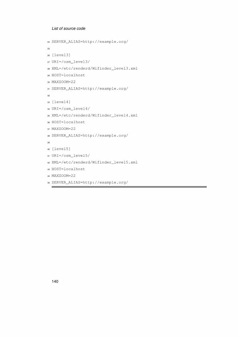
List of source code
24 SERVER_ALIAS=http://example.org/
25
26 [level3]
27 URI=/osm_level3/
28 XML=/etc/renderd/Wifinder_level3.xml
29 HOST=localhost
30 MAXZOOM=22
31 SERVER_ALIAS=http://example.org/
32
33 [level4]
34 URI=/osm_level4/
35 XML=/etc/renderd/Wifinder_level4.xml
36 HOST=localhost
37 MAXZOOM=22
38 SERVER_ALIAS=http://example.org/
39
40 [level5]
41 URI=/osm_level5/
42 XML=/etc/renderd/Wifinder_level5.xml
43 HOST=localhost
44 MAXZOOM=22
45 SERVER_ALIAS=http://example.org/
140

D.2
Web
servicecode
D.2 Web service code
Listing D.5: Python code to calculate the position of a device
1 @app.route(’/getLocation’, methods=[’GET’, ’POST’])
2 def wifiPosition():
3 """
4 Calculate the approximate position of a device that transmits a signal
5 scan.
6
7 :return:
8 """
9
10 # Threshold Parameter:
11 TP1 = -85
12 TP2 = -80
13 TP3 = -70
14 apThreshold = 3
15 #of signalNodes averaged into location
16 neighbours = 5
17
18 if request.method == ’GET’:
19 query = g.db.query(SignalNode)
20 query = query.all()
141

Listofsourcecode
21
22 if app.config[’DEBUG’]:
23 print(’List of wifi signals %s’ % query[0])
24
25 return jsonify(miau=query[0].to_dict())
26
27 if request.method == ’POST’:
28 js = request.json
29
30 posScan = js[’position_scan’]
31
32 # Values for location heuristic
33 lastLatitude = posScan[’last_latitude’]
34 lastLongitude = posScan[’last_longitude’]
35 last_level = posScan[’last_level’]
36
37 mPosScan = []
38
39 print(’Delete APs with signal strength lower %s ’ % TP1)
40 # remove Signals < threshold 1
41 for signal in posScan[’signals’]:
42 if signal[’frequency’] > 5000:
43 wifi5 = True
142

D.2
Web
servicecode
44 if signal[’signal_strength’] > TP1:
45 mPosScan.append(signal)
46
47 #5GhZ results available
48 wifi5 = False
49
50 aps = []
51 for signal in mPosScan:
52 print((’add signal {} with signal strength {} to positioning signal’).format(
53 signal[’ap’][’bssid’],
54 signal[’signal_strength’]))
55 aps.append(signal[’ap’][’bssid’])
56
57
58
59
60 ## Get all SignalNodes with the found APs
61 query = g.db.query(SignalNode)
62 query = query.filter(Signal.ap_bssid.in_(aps)).all()
63
64 positionList = []
65
66 #calculate euclidean distance:
143

Listofsourcecode
67
68 #iterate over all found calibration nodes
69 for calibrationNode in query:
70
71
72 ap_counter = 0
73 distance_vector = 0
74 print((’Checking Calibration Node {}’).format(calibrationNode.to_dict()))
75
76 # iterate over position scan signals
77 for positionSignal in mPosScan:
78
79 #Check if BS with signal strength > TP3 exists in this calibrationNode
80 exists = True
81 if positionSignal[’signal_strength’] > TP3:
82 exists = False
83 for calibrationSignal in calibrationNode.signals:
84 if calibrationSignal.ap_bssid == positionSignal[’ap’][’bssid’]:
85 exists = True
86
87 if not exists:
88 # no check if 5GHZ
89 #if positionSignal[’frequency’] > 5 and not wifi5:
144

D.2
Web
servicecode
90 # pass
91 #Signal strength is larger then TP3, calibration node ist
92 # not used for locating
93 print((’AP {} with signal strength {} is above TP3 of {}’).format(
94 positionSignal[’ap’],
95 positionSignal[’signal_strength’],
96 TP3))
97 break
98
99 else:
100 for calibrationSignal in calibrationNode.signals:
101 if positionSignal[’ap’][’bssid’] == calibrationSignal.ap_bssid:
102 print(
103 (’adding positionSignal of {} to distance_vector’).format(
104 positionSignal[’ap’][’bssid’]))
105 ap_counter = ap_counter + 1
106 distance = calibrationSignal.signal_strength\
107 -positionSignal[’signal_strength’]
108 distance = math.pow(distance, 2)
109 distance_vector = distance + distance_vector
110 else:
111 #no breaks encountered
112 continue
145

Listofsourcecode
113 break
114 else:
115 if ap_counter > apThreshold:
116 euclidian_distance = math.sqrt(distance_vector / ap_counter)
117 print(’Euclidian Distance: %s’ % euclidian_distance)
118 tuple = euclidian_distance, calibrationNode
119 positionList.append(tuple)
120 continue
121
122
123 ##TODO: correct message if list too small
124 if len(positionList) < 1:
125 response = Response(status=500)
126 return response
127
128 positionList.sort()
129 if True:
130 for k, v in positionList:
131 print(’Distance {} for Node {} ’).format(k, v.to_dict())
132
133 distance, bestSignalNode = positionList[0]
134
135
146

D.2
Web
servicecode
136
137 location = [[’latitude’, bestSignalNode.latitude],
138 [’longitude’, bestSignalNode.longitude],
139 [’level’, bestSignalNode.level]]
140 print((’Location of best signal node: {}’).format(location))
141
142 #initialize counting variables
143 index = 0
144 latitude = 0
145 longitude = 0
146 distances = 0
147 level = 0
148 level_sum = 0
149
150 for distance, node in positionList:
151 if index >= neighbours:
152 break
153
154 index = index + 1
155 distances = (1 / distance) + distances
156 latitude = (node.latitude / distance) + latitude
157 longitude = (node.longitude / distance) + longitude
158 level = (node.level / distance) + level
147

Listofsourcecode
159
160 latitude = latitude / distances
161 longitude = longitude / distances
162 level = level / distances
163 print((’average level {}’).format(level))
164 level = round(level, 0)
165
166 location = [[’latitude’, latitude], [’longitude’, longitude], [’level’, level]]
167
168 print(’Average location: {} ’).format(location)
169
170 return jsonify(location)
171
172
173 # TODO: Return a URL to the uploaded object
174 resp = Response(status=200)
175 return resp
Listing D.6: Python implementation of Dijkstra’s algorithm
1 from sqlalchemy import *
2 from sqlalchemy.dialects.postgresql import array
3 from sqlalchemy.types import BigInteger
148

D.2
Web
servicecode
4 from sqlalchemy import func
5
6 from shapely.geometry import Point
7
8 from geoalchemy2.elements import WKTElement
9
10 from uulm_find.database import db_session
11 from uulm_find.models.osm import *
12 from uulm_find import app
13 from itertools import chain
14
15
16 __author__ = ’Alexander Bachmeier’
17
18
19 class Routing:
20 def init(self, g):
21 #Get the g object from the current flask request (allows us to perform database queries)
22 #self.g = g
23 self.db = g.db
24 self.metadata = MetaData()
25
26 pass
149

Listofsourcecode
27
28
29 def getWays(self, level):
30 query = db.query(Ways).filter(
31 and_(Ways.tags[’level’] == level, Ways.tags[’highway’] == ’corridor’))
32
33 return query
34
35
36 def get_neighbour_nodes(self, nodeId):
37 """
38 Returns a list of nodes with the id of all neighbours of the given node
39 :param node:
40 :return: list of node ids
41 """
42 if app.config[’DEBUG’]:
43 print("getNeighourNodes Start")
44
45 ## Get all ways the starting node is on:
46 ## select * from ways where nodes @> ’-710’::bigint[];
47
48 ways_with_node = self.db.query(Ways).filter(
49 and_(Ways.nodes.contains(array([cast(nodeId, BigInteger)])),
150

D.2
Web
servicecode
50 or_(Ways.tags[’highway’] == ’corridor’, Ways.tags[’highway’] == ’steps’),
51 not_(Ways.tags.has_key(’area’)))).all()
52
53 neighbour_ids = []
54
55 #Traverse ways with nods
56 for way in ways_with_node:
57 if app.config[’DEBUG’]:
58 print(
59 ("Getting neighbour nodes of {0} on way with id: {1}").format(nodeId,
60 way.id))
61 #get seq# of "node" on current way:
62 way_node = self.db.query(WayNodes).filter(
63 and_(WayNodes.way_id == way.id, WayNodes.node_id == nodeId)).one()
64 node_seq = way_node.sequence_id
65
66 #get all nodes on way
67 all_way_nodes = self.db.query(WayNodes).filter(
68 WayNodes.way_id == way.id).all()
69
70 ##check if nodes are -1 or +1 in seq from "node"
71 for way_node in all_way_nodes:
72 if way_node.sequence_id == (node_seq + 1) or way_node.sequence_id == (
151

Listofsourcecode
73 node_seq - 1):
74 neighbour_ids.append(int(way_node.node_id))
75
76 if app.config[’DEBUG’]:
77 print(
78 ("List of neighbours of node with id {0}: {1}").format(nodeId, neighbour_ids))
79 print("getNeighourNodes END")
80
81 return neighbour_ids
82
83
84 def getDistance(self, node1_id, node2_id):
85 """
86 Calculate the distance between two nodes
87 :param node1_id: id of the first node
88 :param node2_id: id of the second node
89 :return: distance as a geom object between the two nodes
90 """
91 node1 = self.db.query(Nodes).get(node1_id)
92 node2 = self.db.query(Nodes).get(node2_id)
93
94 query = self.db.query(func.ST_DISTANCE(node1.geom, node2.geom)).one()
95 if app.config[’DEBUG’]:
152

D.2
Web
servicecode
96 print(
97 ("distance between node {0} and node {1}: {2}").format(node1_id, node2_id,
98 query))
99
100 return query[0]
101
102
103 def dijkstra(self, startNode, endNode):
104 """
105 Dijkstra algorithm that returns the shortest path from startNode to endNode
106 :param startNode: uulm_find.models.osm.Node object
107 :param endNode: uulm_find.models.osm.Node object
108 """
109
110 distance = {} #distance
111 best_prev_node = {}
112
113 distance[startNode.id] = 0 ##distance to start node = 0
114
115 #add starting nodes to queue
116 queue = []
117 queue.append(startNode.id)
118
153

Listofsourcecode
119 #the algorithm itself only uses the ID of the nodes,
120 #not the actual representation of the node!
121
122 #while loop counter
123 count = 0
124 #make sure code doesn’t run forever
125 max_count = 100000
126
127 while count < max_count:
128 if app.config[’DEBUG’]:
129 print((’While counter : {0}’).format(count))
130 count = count + 1
131
132 try:
133 current_node = queue.pop(0)
134 except IndexError:
135 print("IndexError")
136 break
137
138 if current_node == endNode.id:
139 ##our endNode has been found ==> shortest path found
140 print("Found End Node!")
141 return best_prev_node, distance
154

D.2
Web
servicecode
142
143 #"usual" case of find neighbours and calculating their distance
144
145 neighbors = self.get_neighbour_nodes(current_node)
146 if app.config[’DEBUG’]:
147 print("Node {0} has {1} Neighbours".format(current_node, len(neighbors)))
148
149 for nodeId in neighbors:
150 #append new neighbors to the queue
151 if nodeId not in distance:
152 queue.append(nodeId) ##TODO: might lead to longer routes!
153
154 dist = distance[current_node] + self.getDistance(current_node, nodeId)
155
156 if nodeId in distance:
157 if dist < distance[nodeId]:
158 ##shorter path found, update!
159 distance[nodeId] = dist
160 best_prev_node[nodeId] = current_node
161 else:
162 distance[nodeId] = dist
163 best_prev_node[nodeId] = current_node
164
155

Listofsourcecode
165
166 def getRoute(self, startNode, endNode):
167 print("Start Node ID {0}: \n {1}".format(startNode.id, startNode.to_dict()))
168 print("End Node ID {0}: \n {1}".format(endNode.id, endNode.to_dict()))
169
170 print(’Neighbors of EndNode: {0}’.format(self.get_neighbour_nodes(endNode.id)))
171
172 best_prev_node, distance = self.dijkstra(startNode, endNode)
173
174 route = []
175 loop_node_id = endNode.id
176 while 1:
177 #route complete if previous node is start node:
178 node = self.db.query(Nodes).get(loop_node_id)
179 #
180 # if node.tags[’highway’] is ’steps’:
181 # steps = True
182 # else:
183 # steps = False
184 node_dict = node.to_dict()
185 waypoint = {
186 ’latitude’: node_dict[’latitude’],
187 ’longitude’: node_dict[’longitude’],
156

D.2
Web
servicecode
188 ’level’: node_dict[’level’],
189 ’steps’: False,
190 }
191
192 route.insert(0, waypoint)
193 if (best_prev_node[loop_node_id] == int(startNode.id)):
194 break
195 loop_node_id = best_prev_node[loop_node_id]
196
197 ##close database collection
198 #db.close()
199
200 print(’Finished Route:’)
201 for waypoint in route:
202 print(waypoint)
203
204 #Return a route, represented by a list of waypoints.
205 #Starting from the StartNode to the EndNode
206 return route
207
208
209 def getNextWayNode(self, location):
210
157

Listofsourcecode
211
212 # Create a geometry point; arguments are lon, lat
213 point = ’Point(%0.8f %0.8f)’ % (location[’longitude’], location[’latitude’])
214
215 # transform into a wkt element
216 wkt_point = WKTElement(
217 ’Point({0} {1})’.format(location[’longitude’], location[’latitude’]),
218 srid=4326)
219
220 #get a list of all way nodes
221 listOfNodes = self.db.query(Ways.nodes).filter(
222 and_(Ways.tags[’highway’] == ’corridor’),
223 % Ways.tags[’level’] == str(location[’level’])).order_by(
224 Ways.bbox.distance_box(wkt_point)).all()
225
226
227 #flatten list of lists of lists:
228 node_ids = list(chain.from_iterable((chain.from_iterable(listOfNodes))))
229
230 best_node = self.db.query(Nodes).filter(Nodes.id.in_(node_ids)).order_by(
231 Nodes.geom.distance_box(wkt_point)).first()
232
233
158

D.2
Web
servicecode
234 return best_node
235
236
237 if __name__ == ’__main__’:
238 db = db_session()
239
240 routing = Routing()
241 routing.db = db
242 #routing.getRoute(node1, node2)
243 current_location = {’latitude’: 48.4228724245706, ’longitude’: 9.95691005140543,
244 ’level’: 2}
245
246 routing.getNextWayNode(current_location)
247
248
249
250 #g.db.close()
159

List of source code
D.3 OsmConverter
These tools are used to upload OSM data into the webservice’s database. The data is
used for POI services as well as routing.
Listing D.7: OsmConvert.py, used to add missing information from OSM XML data
1 #!/usr/bin/env python2
2
3 __author__ = ’Alexander Bachmeier’
4 # add missing version attribute from JOSM osm exports
5 import xml.etree.ElementTree as ET
6 from datetime import datetime
7
8
9 INPUT_FILE = ’uulm.osm’
10 OUTPUT_FILE = ’osm_output.xml’
11
12
13 #get input file using ElementTree parser
14 tree = ET.parse(INPUT_FILE)
15 root = tree.getroot()
16
17 #timestamp format: timestamp="2012-06-04T21:25:04Z"
18 now = datetime.datetime.now()
19 timestamp = now.strftime("%Y-%m-%dT%H:%M:%SZ")
20
21 #traverse children
22 for child in root:
23 #add required version attribute
24 if child.tag == ’node’ or child.tag == ’way’ or \
25 child.tag == ’relation’\
26 and ’version’ not in child.attrib:
27 child.set(’version’, ’0’)
160

D.3 OsmConverter
28 #add required timestamp attribute
29 if child.tag == ’node’ or child.tag == ’way’ or \
30 child.tag == ’relation’ \
31 and ’timestamp’ not in child.attrib:
32 child.set(’timestamp’, timestamp)
33
34 tree.write(OUTPUT_FILE)
Listing D.8: Tool to automate process
1 #!/bin/bash
2
3
4 ./OsmConvert.py
5 #Truncate Database before import
6 osmosis --tp user="osm" database="osm" \
7 password="$PASSWORD" \
8 host="example.org" \
9
10
11 osmosis --read-xml file="osm_output.xml" \
12 --write-pgsql user="USER" database="osm" \
13 password="$PASSWORD" host="example.org"
161


Name: B. Sc. Alexander Bachmeier Matrikelnummer: 628453
Erklärung
Ich erkläre, dass ich die Arbeit selbständig verfasst und keine anderen als die angegebe-
nen Quellen und Hilfsmittel verwendet habe.
Ulm, den . . . . . . . . . . . . . . . . . . . . . . . . . . . . . . . . . . . . . . . . . . . . . . . . . . . . . . . . . . . . . . . . . . . . . . . . . . . .
B. Sc. Alexander Bachmeier


![Using Robots and SLAM for Indoor Wi-Fi Mapping in …1 Using Robots and SLAM for Indoor Wi-Fi Mapping in Indoor Geolocation [Extended Report] A Major Qualifying Project Report Submitted](https://static.fdocuments.in/doc/165x107/5f5a3f0946954b67e9462c68/using-robots-and-slam-for-indoor-wi-fi-mapping-in-1-using-robots-and-slam-for-indoor.jpg)