Why Outlet Stores Exist:

Averting Cannibalization in Product Line Extensions

Donald Ngwe∗

September 30, 2016

Abstract

Outlet stores offer attractive prices at locations far from central shopping districts.They form a large and growing component of many firms’ retailing strategies, partic-ularly in the fashion industry. The main perspectives on why outlet stores exist canbe broadly classified into inventory management, geographic segmentation, and pricediscrimination through consumer self-selection. I evaluate these perspectives in thecontext of a major fashion goods firm using newly available and highly granular data.Model-free evidence shows that inventory management and geographic segmentationdo not fully explain the benefit of selling through outlet stores. Consumers who shopat outlet stores also do not differ significantly from those who shop at regular storesin terms of income. I use a structural demand model to show that consumers are seg-mented according to their sensitivity to travel distance and taste for product newness.I then develop a supply model to predict product development responses to changes instore locations. Through policy simulations, I discover that the firm uses outlet storesto serve lower-value consumers who self-select by traveling to outlet stores from cen-tral shopping districts. The firm sells older, less desirable merchandise through outletstores to prevent cannibalization of regular store revenues by means of exploiting thepositive correlation between consumers’ travel sensitivity and taste for new products.I find that the rate of new product introduction in regular stores would fall by 16%if outlet stores were closed down, while variable profits would decline by 23%. Theseresults imply that the existence of outlet stores may enable firms to improve quality intheir regular channels, thus counteracting brand dilution effects.

∗Email: dngwe@hbs.edu. This paper is based on my dissertation. I am grateful to my dissertationcommittee members Chris Conlon, Brett Gordon, Kate Ho, Mike Riordan, and Scott Shriver for theirguidance and encouragement. I also thank Jonathan Dingel, Paul Grieco, Jessie Handbury, Oded Netzer,Bernard Salanie, David Soberman, Patrick Sun, Olivier Toubia, and participants of Columbia’s industrialorganization colloquium for helpful comments and suggestions. All errors are my own.

1

1 Introduction

Outlet stores are a fixture of the American retail landscape. These brick-and-mortar stores

offer deep discounts in locations far away from most consumers. Firms operate outlet stores

in addition to regular stores, which are located in central shopping districts. Outlet stores

operated by different firms are often agglomerated in sprawling outlet malls off interstate

highways. As of March 2014 there were 201 outlet malls in North America, which generated

an estimated $31-42 billion in annual revenues (Humphers, 2014). This is a large and growing

portion of total retail sales in clothing and clothing accessories, which amounted to $241

billion in 2012.1

There are several perspectives on why outlet stores have become a widely adopted selling

strategy. One concerns inventory management : outlet stores provide firms with a cost-

efficient way to dispose of excess inventory. Another is geographic segmentation: outlet

stores cater to lower-value consumers that reside near outlet malls. A third is consumer

self-selection: lower-value consumers are more willing to travel greater distances to avail of

discounted products.2

The multiplicity of views on why outlet stores exist corresponds to the variety of ways

in which firms sell through outlet stores, a sense of which is provided by a report from

ConsumerReports.org:

When we asked outlet-store employees and customer-service reps for differences be-

tween goods at their chain’s outlet and retail stores, they were candid, and it’s clear

that every company has its own strategy. Staff at Under Armour told us that the

outlets sell older merchandise from regular stores and goods made just for the outlets.

A Guess employee explained it fills its shelves with discontinued items, while a worker

1A second, mutually exclusive comparison is to annual department store sales, which was $183 billion in2012. Both figures are from the 2012 US Economic Census.

2Yet another perspective is that outlet stores lower search costs for consumers through collocation. Whilethis is likely to be true, collocation is also a common feature among regular stores. This paper focuses onfeatures of outlet stores that distinguish them from regular stores.

2

at Gap said the chain offers apparel that never saw the light of day in a regular store.

At Black & Decker Factory Stores, you’ll find fully warranted demo and refurbished

equipment and brand-new goods. Lands’ End “Inlets” carry year-old inventory, clear-

ance items, and returns. Harry & David outlets sell a lot of the food and gifts in the

company’s catalog and on its website (though not always fruit), but prices and promo-

tions differ. Sunglass Hut offers a mix of old and new glasses at “prices not necessarily

cheaper” than those at its mall-based stores, a customer-service representative told

us. Some retailers don’t draw any line between outlet and regular merchandise. A

customer-service rep for Dress Barn told us that in all the company’s stores, “it’s the

exact same stuff, just different prices and promotions.”3

In this paper, I evaluate the relevance of several possible reasons for selling through outlet

stores in the case of a major fashion goods firm with a heavy outlet store presence. Using

newly available and highly granular data, I am able to observe both inventory flows between

store formats, and locations and sales records of individual consumers—rich sources of model-

free evidence. I then use a structural model of demand and supply to predict consumer

behavior and firm product decisions under counterfactual distribution schemes.

It is evident from observing product flows and production runs that inventory management

is not the sole function of the firm’s outlet stores. The firm sells a significant fraction of units

of each style through the outlet channel. It is also immediately clear that outlet stores do

not mainly serve consumers who reside in their vicinity—most of each outlet store’s revenues

are attributed to consumers for whom a regular store is closer to home. This suggests that

the firm’s main motivation for operating outlet stores might be to price discriminate between

its consumers by forcing the most price-sensitive among them to travel to obtain discounts.

Notably, consumers who shop at outlet stores do not differ significantly from consumers who

shop at regular stores in terms of observable characteristics such as income. They make

3“Outlet Malls Then and Now.” http://www.consumerreports.org/cro/magazine-archive/2011/

november/shopping/outlet-stores/outlet-malls-then-and-now/index.htm. Accessed 9-13-2015.

3

purchases at roughly the same frequency, and have had about the same time elapse since

their first purchase of the brand. Taking these factors into account, I propose a demand

model that characterizes how consumers make their purchase decisions. I use the demand

model to estimate the extent to which consumers vary in their unobservable characteristics,

and to show that outlet store consumers significantly differ from regular store consumers

in two ways: their sensitivity to travel distance and their taste for product newness. In

addition, I find a strong positive correlation between these two values.

I hypothesize that the firm exploits the positive correlation between consumer travel sensi-

tivity and taste for new products by selling older products in its outlet stores. I test this

notion by setting the correlation to zero and simulating the corresponding purchase behavior.

I find that the resulting advantage to operating outlet stores is much diminished, owing to

the fact that outlet stores would cannibalize a larger portion of regular store revenues.

In order to better characterize the consumer’s choice set in the absence of outlet stores, I

build a supply model in which the firm optimally sets prices and product introduction rates

given store locations. While prices can be adequately modeled using a standard monopoly

pricing assumption, modeling the firm’s product choice presents a nontrivial challenge. I

address the problem by developing a probabilistic model of product choice. Rather than

requiring the firm to choose characteristics individually for each of hundreds of products, I

describe the firm’s choice set in terms of a joint probability distribution of characteristics.

The firm’s problem can then be reduced to choosing the parameters of this distribution.

Since product ages are of particular importance to consumers, I focus on the firm’s choice

of the rate of product introductions and reassignment to outlets, which are arguably the

components of product quality over which the firm has the highest degree of control.

I find that the firm is able to serve a much narrower range of consumers in the absence of

outlet stores. With only its regular distribution channel available, the firm would expand its

regular retail audience by lowering prices and the rate of product introduction (and hence

4

the average age) of its products, but would be unable to attain the same level of coverage

without the geographic differentiation enabled by outlets. This reveals an additional benefit

of having outlet stores: they enable the firm to increase its rate of product introduction in the

regular format. I find that the firm introduces 16% more new styles with dual distribution

than with only regular stores. This result implies that the existence of outlet stores may

enable firms to improve quality in their regular channels, thus counteracting brand dilution

effects.

The paper proceeds as follows. I review the related literature in Section 2. In Section 3, I

describe the data. In Section 4, I provide preliminary evidence of how outlet stores work. In

Section 5, I describe the demand model I use to estimate preferences, discuss the estimation

procedure, and present the estimates. In Section 6, I describe the supply model I use to

represent firm product choice, and present the implied marginal and product development

costs. In Section 7, I perform policy simulations that highlight the benefit of operating outlet

stores. Section 8 concludes.

2 Related literature

Prior research puts forth several theories about why firms sell goods through outlet stores.

Deneckere and McAfee (1996) derive conditions under which a firm would damage or “crimp”

a portion of its goods to increase profits by expanding its market coverage, and offer outlet

stores as an example of such a damaged goods strategy. Coughlan and Soberman (2005)

show that dual distribution (i.e. having both regular and outlet stores) is more profitable

than single channel distribution when the range of service sensitivity is low relative to the

range of price sensitivity. Qian et al. (2013) show that the opening of an outlet store had

substantial positive spillovers for a retailer’s catalog and online channels, whereas Soysal and

Krishnamurthi (2015) show that regular physical channels experience these benefits as well.

5

My work complements this literature by applying insights from multidimensional screening

in assessing the relevance to dual distribution of consumer travel costs and taste for quality.

Additionally, I show how having outlet stores impacts overall product assortment.

More generally, this paper offers a new point of view on how product lines should be designed

to effectively segment consumers. Previous work on product line design has explored the ben-

efits of broadening product lines (Kekre and Srinivasan (1990); Bayus and Putsis (1999)),

methods for selecting optimal product lines (Moorthy (1984); Green and Krieger (1985);

McBride and Zufryden (1988); Dobson and Kalish (1988); Netessine and Taylor (2007)), can-

nibalization between product lines (Desai (2001)), pricing (Reibstein and Gatignon (1984);

Draganska and Jain (2006)), and the effects on brand equity of product line extensions

(Randall et al. (1998)). My paper contributes to this body of work by demonstrating the

importance of correlations in consumer tastes in making product line decisions. It also shows

how cannibalization can be mitigated by appropriately combining product line attributes.

I develop an explicit model of product line choice that corresponds to the institutional details

of the fashion goods industry. The large number of products in each product line poses

a particular challenge. While existing work has modeled endogenous product choice for a

single multidimensional good (Fan (2010)) or for several single-dimensional goods (Draganska

et al. (2009); Crawford et al. (2011)), none has addressed the product choice problem of a

firm with several multidimensional products. I introduce a simple and tractable method

of describing this choice. Modeling the firm as choosing the parameters of a distribution of

product characteristics, rather than the characteristics that make up each individual product,

dramatically reduces the number of choice variables for the firm. It is also a more realistic

representation of decision-making in many sectors.

This paper’s central premise is that the choice of whether to open outlet stores and what to

stock them with is a type of multidimensional screening problem. Empirical models of mul-

tidimensional product choice are particularly useful because they can be used to complement

6

lessons from theoretical work in multidimensional screening. The obstacles to obtaining gen-

eral results in multidimensional screening are well-documented by Rochet and Stole (2003).

Full solutions to this problem are available for the discrete two-type case (Armstrong and

Rochet (1999)) and other cases for which the form of consumer heterogeneity is severely

restricted (e.g. Armstrong (1996)). It is difficult to see how these models’ predictions would

manifest in actual product decisions, such as those in my empirical setting. By using de-

mand and supply models that are not anchored to any particular screening model, I am able

to provide evidence for the applicability of existing results to real world settings and the

significance of multidimensional screening for firms in general.

3 Data and industry background

The first outlet stores appeared in the United States in the 1930s. These stores were attached

to factories and sold overruns, irregulars, and slightly damaged goods. Outlet stores initially

catered to only the firm’s employees, but the stores’ market audience quickly expanded to

include regular consumers. Until the 1970s, firms continued to use outlet stores primarily

to dispose of excess inventory, even as they began to established them independently of

manufacturing centers (Coughlan and Soberman, 2004).

The modern outlet store has evolved into a considerably different format from its earlier

incarnations. In many ways, outlet store goods now constitute distinct product lines, rather

than mere excess inventory. Many firms design products exclusively for sale in outlet stores

(though they may prefer to limit awareness of the practice among consumers). Revenues

from outlet stores often rival, and sometimes exceed, revenues from a firm’s regular retail

formats.

One feature of the outlet store that remains unchanged is its distance from central shop-

ping districts. In fact, an entire industry of outlet mall operators owes its existence to the

7

prevalence of this selling strategy among clothing and fashion goods retailers. The prac-

tice of selling goods in hard-to-access locations would seem curious were it not so common.

Yet many firms choose not to sell through outlet stores; adoption is variable even within

narrowly-defined categories. For instance, premium apparel brands Brooks Brothers, Hugo

Boss, and Ralph Lauren have several outlet store locations, but Chanel, Burberry, and Zegna

have few or none.

Data for this project is provided by a major fashion manufacturer and retailer based in the

U.S. The firm’s main product line belongs to a category that generates annual revenues of

about $9 billion in the US. The firm is the market leader, with between 30 and 40 percent

market share. About 60% of the firm’s revenues are sourced from sales of its main product

line. The data used for this study consists of transaction-level records from July 2006 to

March 2011. The sample includes all purchases of products made by U.S. consumers in firm-

operated channels. Excluded from this sample are online and department store transactions,

which according to the firm’s managers accounted for less than 10% of total revenue.

The firm is able to track repeat purchase behavior by consumers. Available information on

consumers includes their billing zip codes, date of first purchase within the brand, and their

total lifetime expenditures on the firm’s products. Each record contains detailed information

on the consumer, the product, and the store. Product attributes include color, silhouette,

materials, collection, release date, and a code that uniquely identifies each style. Store

attributes include their location, weeklong foot traffic, and format type.

For the analysis in this paper, I focus on main category purchases in physical stores. While

this excludes a considerable number of non-main category purchases, those observations are

used to proxy for the number of consumers who visit a store but do not make a purchase in

the main category. Table 1 lists summary statistics of the data set.

The firm’s overall distribution strategy is fairly common among brands with outlet store

locations. The firm introduces most of its new products in its regular stores, which are

8

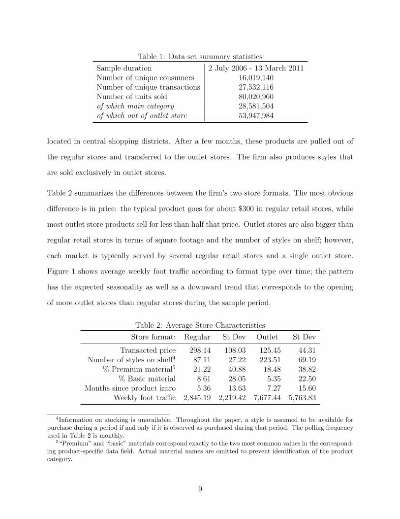
Table 1: Data set summary statistics

Sample duration 2 July 2006 - 13 March 2011Number of unique consumers 16,019,140Number of unique transactions 27,532,116Number of units sold 80,020,960of which main category 28,581,504of which out of outlet store 53,947,984

located in central shopping districts. After a few months, these products are pulled out of

the regular stores and transferred to the outlet stores. The firm also produces styles that

are sold exclusively in outlet stores.

Table 2 summarizes the differences between the firm’s two store formats. The most obvious

difference is in price: the typical product goes for about $300 in regular retail stores, while

most outlet store products sell for less than half that price. Outlet stores are also bigger than

regular retail stores in terms of square footage and the number of styles on shelf; however,

each market is typically served by several regular retail stores and a single outlet store.

Figure 1 shows average weekly foot traffic according to format type over time; the pattern

has the expected seasonality as well as a downward trend that corresponds to the opening

of more outlet stores than regular stores during the sample period.

Table 2: Average Store Characteristics

Store format: Regular St Dev Outlet St Dev

Transacted price 298.14 108.03 125.45 44.31Number of styles on shelf4 87.11 27.22 223.51 69.19

% Premium material5 21.22 40.88 18.48 38.82% Basic material 8.61 28.05 5.35 22.50

Months since product intro 5.36 13.63 7.27 15.60Weekly foot traffic 2,845.19 2,219.42 7,677.44 5,763.83

4Information on stocking is unavailable. Throughout the paper, a style is assumed to be available forpurchase during a period if and only if it is observed as purchased during that period. The polling frequencyused in Table 2 is monthly.

5“Premium” and “basic” materials correspond exactly to the two most common values in the correspond-ing product-specific data field. Actual material names are omitted to prevent identification of the productcategory.

9

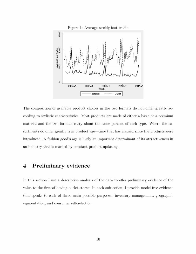
Figure 1: Average weekly foot traffic

The composition of available product choices in the two formats do not differ greatly ac-

cording to stylistic characteristics. Most products are made of either a basic or a premium

material and the two formats carry about the same percent of each type. Where the as-

sortments do differ greatly is in product age—time that has elapsed since the products were

introduced. A fashion good’s age is likely an important determinant of its attractiveness in

an industry that is marked by constant product updating.

4 Preliminary evidence

In this section I use a descriptive analysis of the data to offer preliminary evidence of the

value to the firm of having outlet stores. In each subsection, I provide model-free evidence

that speaks to each of three main possible purposes: inventory management, geographic

segmentation, and consumer self-selection.

10

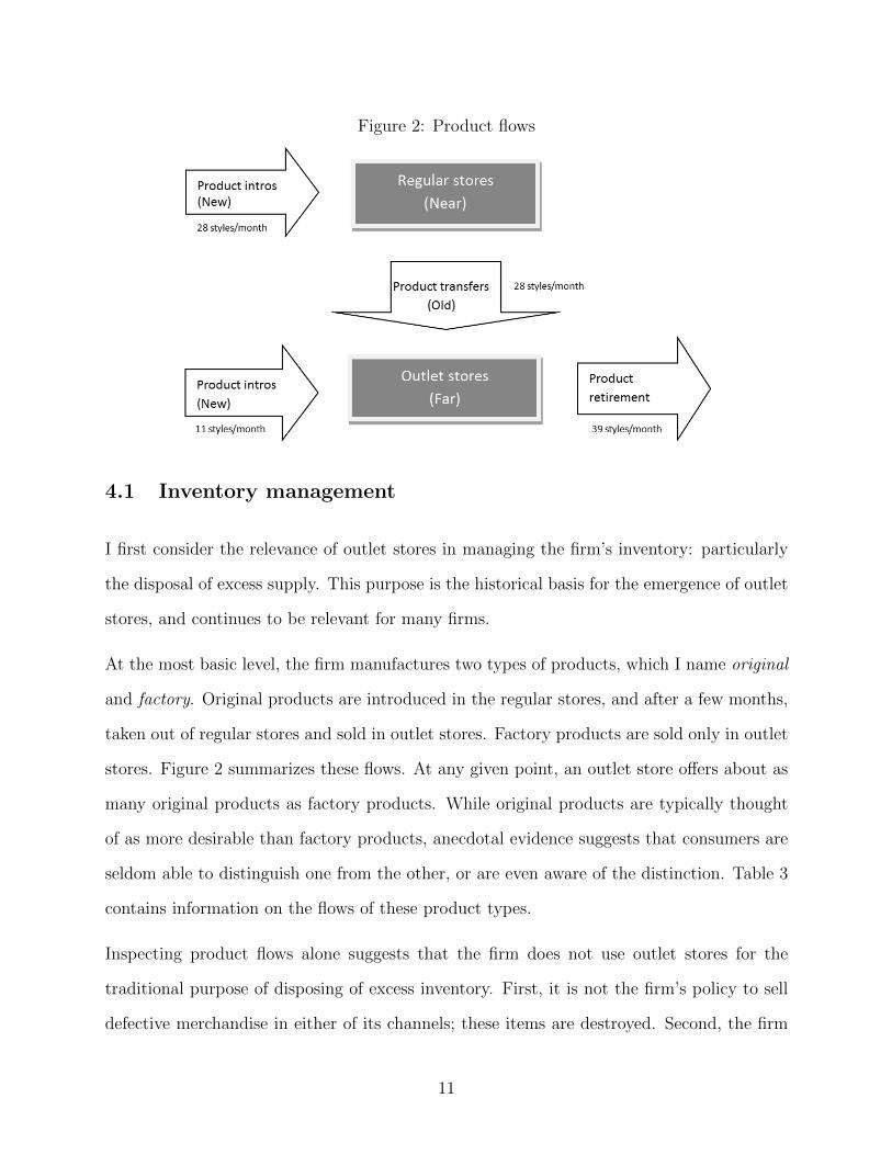
Figure 2: Product flows

4.1 Inventory management

I first consider the relevance of outlet stores in managing the firm’s inventory: particularly

the disposal of excess supply. This purpose is the historical basis for the emergence of outlet

stores, and continues to be relevant for many firms.

At the most basic level, the firm manufactures two types of products, which I name original

and factory. Original products are introduced in the regular stores, and after a few months,

taken out of regular stores and sold in outlet stores. Factory products are sold only in outlet

stores. Figure 2 summarizes these flows. At any given point, an outlet store offers about as

many original products as factory products. While original products are typically thought

of as more desirable than factory products, anecdotal evidence suggests that consumers are

seldom able to distinguish one from the other, or are even aware of the distinction. Table 3

contains information on the flows of these product types.

Inspecting product flows alone suggests that the firm does not use outlet stores for the

traditional purpose of disposing of excess inventory. First, it is not the firm’s policy to sell

defective merchandise in either of its channels; these items are destroyed. Second, the firm

11

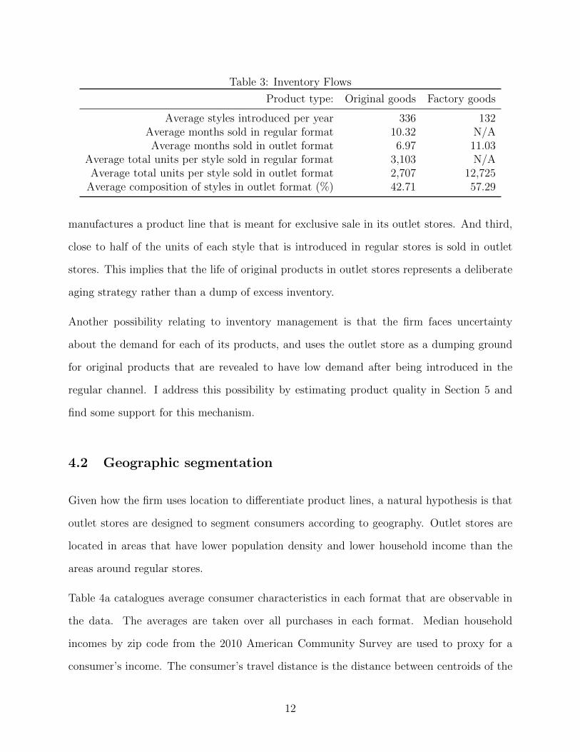
Table 3: Inventory Flows

Product type: Original goods Factory goods

Average styles introduced per year 336 132Average months sold in regular format 10.32 N/AAverage months sold in outlet format 6.97 11.03

Average total units per style sold in regular format 3,103 N/AAverage total units per style sold in outlet format 2,707 12,725

Average composition of styles in outlet format (%) 42.71 57.29

manufactures a product line that is meant for exclusive sale in its outlet stores. And third,

close to half of the units of each style that is introduced in regular stores is sold in outlet

stores. This implies that the life of original products in outlet stores represents a deliberate

aging strategy rather than a dump of excess inventory.

Another possibility relating to inventory management is that the firm faces uncertainty

about the demand for each of its products, and uses the outlet store as a dumping ground

for original products that are revealed to have low demand after being introduced in the

regular channel. I address this possibility by estimating product quality in Section 5 and

find some support for this mechanism.

4.2 Geographic segmentation

Given how the firm uses location to differentiate product lines, a natural hypothesis is that

outlet stores are designed to segment consumers according to geography. Outlet stores are

located in areas that have lower population density and lower household income than the

areas around regular stores.

Table 4a catalogues average consumer characteristics in each format that are observable in

the data. The averages are taken over all purchases in each format. Median household

incomes by zip code from the 2010 American Community Survey are used to proxy for a

consumer’s income. The consumer’s travel distance is the distance between centroids of the

12

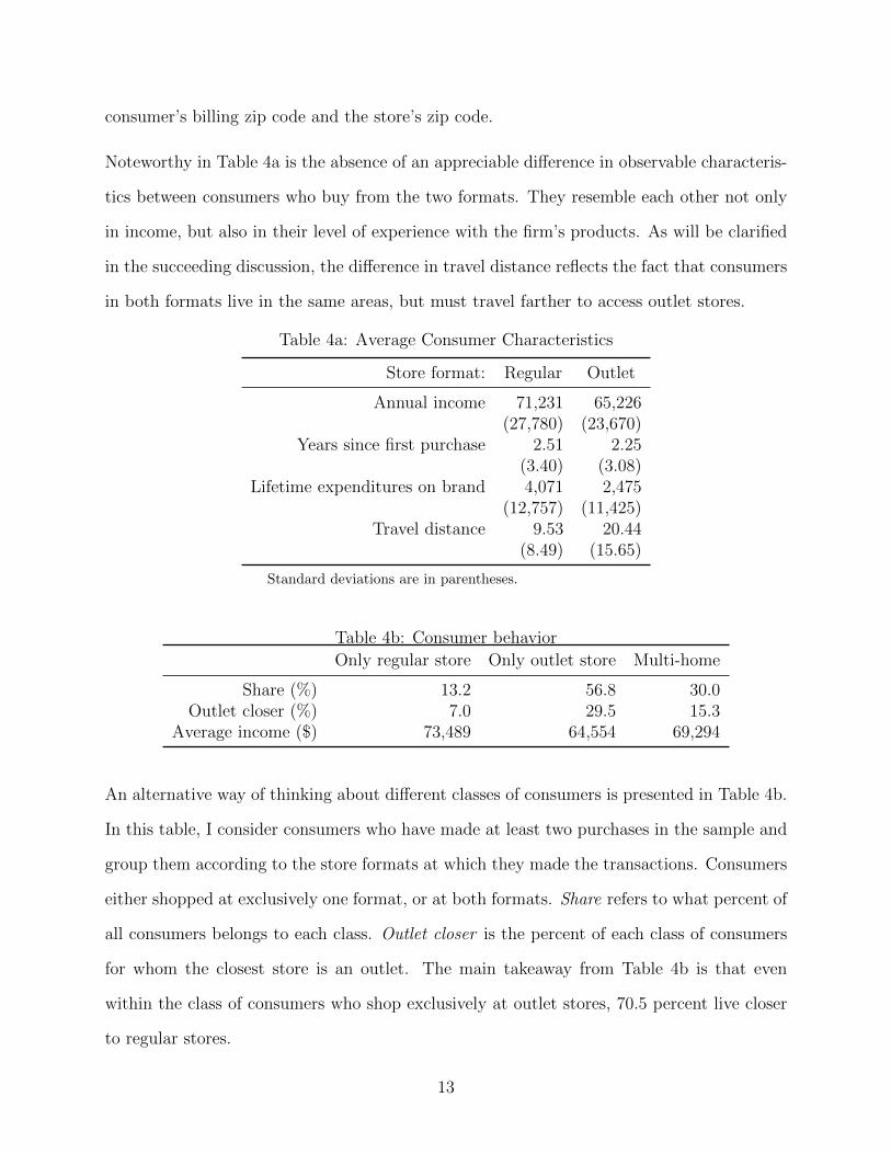
consumer’s billing zip code and the store’s zip code.

Noteworthy in Table 4a is the absence of an appreciable difference in observable characteris-

tics between consumers who buy from the two formats. They resemble each other not only

in income, but also in their level of experience with the firm’s products. As will be clarified

in the succeeding discussion, the difference in travel distance reflects the fact that consumers

in both formats live in the same areas, but must travel farther to access outlet stores.

Table 4a: Average Consumer Characteristics

Store format: Regular Outlet

Annual income 71,231 65,226(27,780) (23,670)

Years since first purchase 2.51 2.25(3.40) (3.08)

Lifetime expenditures on brand 4,071 2,475(12,757) (11,425)

Travel distance 9.53 20.44(8.49) (15.65)

Standard deviations are in parentheses.

Table 4b: Consumer behavior

Only regular store Only outlet store Multi-home

Share (%) 13.2 56.8 30.0Outlet closer (%) 7.0 29.5 15.3

Average income ($) 73,489 64,554 69,294

An alternative way of thinking about different classes of consumers is presented in Table 4b.

In this table, I consider consumers who have made at least two purchases in the sample and

group them according to the store formats at which they made the transactions. Consumers

either shopped at exclusively one format, or at both formats. Share refers to what percent of

all consumers belongs to each class. Outlet closer is the percent of each class of consumers

for whom the closest store is an outlet. The main takeaway from Table 4b is that even

within the class of consumers who shop exclusively at outlet stores, 70.5 percent live closer

to regular stores.

13

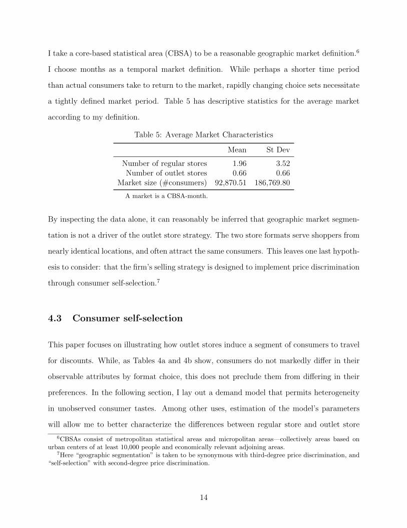
I take a core-based statistical area (CBSA) to be a reasonable geographic market definition.6

I choose months as a temporal market definition. While perhaps a shorter time period

than actual consumers take to return to the market, rapidly changing choice sets necessitate

a tightly defined market period. Table 5 has descriptive statistics for the average market

according to my definition.

Table 5: Average Market Characteristics

Mean St Dev

Number of regular stores 1.96 3.52Number of outlet stores 0.66 0.66

Market size (#consumers) 92,870.51 186,769.80

A market is a CBSA-month.

By inspecting the data alone, it can reasonably be inferred that geographic market segmen-

tation is not a driver of the outlet store strategy. The two store formats serve shoppers from

nearly identical locations, and often attract the same consumers. This leaves one last hypoth-

esis to consider: that the firm’s selling strategy is designed to implement price discrimination

through consumer self-selection.7

4.3 Consumer self-selection

This paper focuses on illustrating how outlet stores induce a segment of consumers to travel

for discounts. While, as Tables 4a and 4b show, consumers do not markedly differ in their

observable attributes by format choice, this does not preclude them from differing in their

preferences. In the following section, I lay out a demand model that permits heterogeneity

in unobserved consumer tastes. Among other uses, estimation of the model’s parameters

will allow me to better characterize the differences between regular store and outlet store

6CBSAs consist of metropolitan statistical areas and micropolitan areas—collectively areas based onurban centers of at least 10,000 people and economically relevant adjoining areas.

7Here “geographic segmentation” is taken to be synonymous with third-degree price discrimination, and“self-selection” with second-degree price discrimination.

14

shoppers. This step illustrates how the firm’s selling strategy achieves a sorting of consumers

according to their preferences.

5 Demand

I present a model of consumer demand that describes store and product choice. I proceed

to discuss how I estimate model parameters using transactions data from the firm. Finally,

I present the results of demand estimation and discuss what they imply about the function

of outlet stores as a tool for price discrimination.

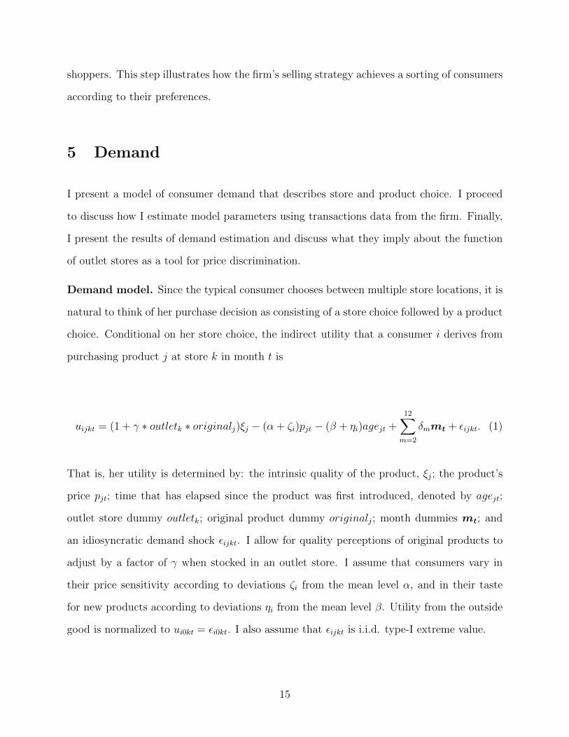
Demand model. Since the typical consumer chooses between multiple store locations, it is

natural to think of her purchase decision as consisting of a store choice followed by a product

choice. Conditional on her store choice, the indirect utility that a consumer i derives from

purchasing product j at store k in month t is

uijkt = (1 + γ ∗ outletk ∗ originalj)ξj − (α + ζi)pjt − (β + ηi)agejt +12∑m=2

δmmt + εijkt. (1)

That is, her utility is determined by: the intrinsic quality of the product, ξj; the product’s

price pjt; time that has elapsed since the product was first introduced, denoted by agejt;

outlet store dummy outletk; original product dummy originalj; month dummies mt; and

an idiosyncratic demand shock εijkt. I allow for quality perceptions of original products to

adjust by a factor of γ when stocked in an outlet store. I assume that consumers vary in

their price sensitivity according to deviations ζi from the mean level α, and in their taste

for new products according to deviations ηi from the mean level β. Utility from the outside

good is normalized to ui0kt = εi0kt. I also assume that εijkt is i.i.d. type-I extreme value.

15

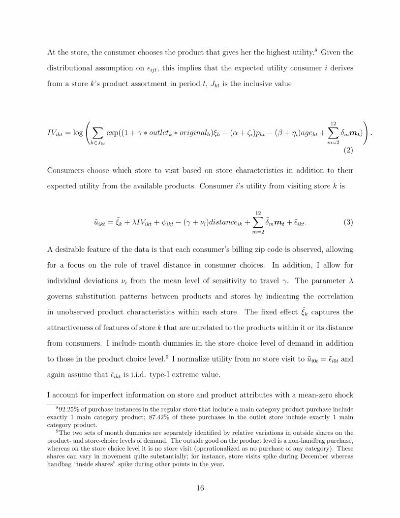
At the store, the consumer chooses the product that gives her the highest utility.8 Given the

distributional assumption on εijt, this implies that the expected utility consumer i derives

from a store k’s product assortment in period t, Jkt is the inclusive value

IVikt = log

(∑h∈Jkt

exp((1 + γ ∗ outletk ∗ originalh)ξh − (α + ζi)pht − (β + ηi)ageht +12∑m=2

δmmt)

).

(2)

Consumers choose which store to visit based on store characteristics in addition to their

expected utility from the available products. Consumer i’s utility from visiting store k is

uikt = ξk + λIVikt + ψikt − (γ + νi)distanceik +12∑m=2

δmmt + εikt. (3)

A desirable feature of the data is that each consumer’s billing zip code is observed, allowing

for a focus on the role of travel distance in consumer choices. In addition, I allow for

individual deviations νi from the mean level of sensitivity to travel γ. The parameter λ

governs substitution patterns between products and stores by indicating the correlation

in unobserved product characteristics within each store. The fixed effect ξk captures the

attractiveness of features of store k that are unrelated to the products within it or its distance

from consumers. I include month dummies in the store choice level of demand in addition

to those in the product choice level.9 I normalize utility from no store visit to ui0t = εi0t and

again assume that εikt is i.i.d. type-I extreme value.

I account for imperfect information on store and product attributes with a mean-zero shock

892.25% of purchase instances in the regular store that include a main category product purchase includeexactly 1 main category product; 87.42% of these purchases in the outlet store include exactly 1 maincategory product.

9The two sets of month dummies are separately identified by relative variations in outside shares on theproduct- and store-choice levels of demand. The outside good on the product level is a non-handbag purchase,whereas on the store choice level it is no store visit (operationalized as no purchase of any category). Theseshares can vary in movement quite substantially; for instance, store visits spike during December whereashandbag “inside shares” spike during other points in the year.

16

ψikt ∼ N(0, σψikt) where σψikt = Xiktβψ is a linear combination of store- and shopper-

specific attributes: an outlet store dummy, travel distance, and time since store opening.10

I choose this functional form and these covariates based on data availability and computa-

tional tractability. The true form of shopper uncertainty is likely to be more complex, with

information depending on various reference points (such as competitors’ offerings, prior ex-

posure, and advertising messages), varying over attributes, and decaying over time.11 I find

that within the current model specification, accounting for individual-level heterogeneity in

shopping experience does not significantly affect the degree of uncertainty (see Appendix E ).

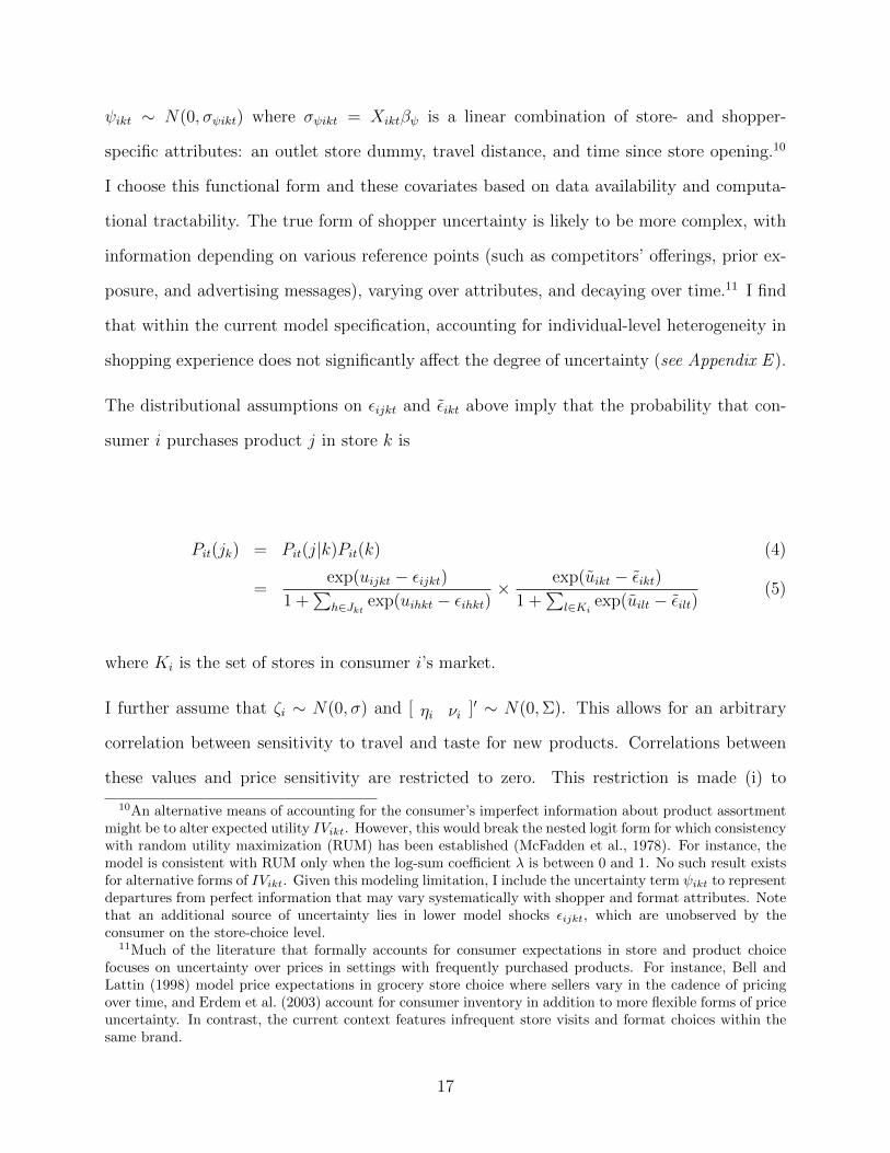
The distributional assumptions on εijkt and εikt above imply that the probability that con-

sumer i purchases product j in store k is

Pit(jk) = Pit(j|k)Pit(k) (4)

=exp(uijkt − εijkt)

1 +∑

h∈Jkt exp(uihkt − εihkt)× exp(uikt − εikt)

1 +∑

l∈Kiexp(uilt − εilt)

(5)

where Ki is the set of stores in consumer i’s market.

I further assume that ζi ∼ N(0, σ) and [ ηi νi ]′ ∼ N(0,Σ). This allows for an arbitrary

correlation between sensitivity to travel and taste for new products. Correlations between

these values and price sensitivity are restricted to zero. This restriction is made (i) to

10An alternative means of accounting for the consumer’s imperfect information about product assortmentmight be to alter expected utility IVikt. However, this would break the nested logit form for which consistencywith random utility maximization (RUM) has been established (McFadden et al., 1978). For instance, themodel is consistent with RUM only when the log-sum coefficient λ is between 0 and 1. No such result existsfor alternative forms of IVikt. Given this modeling limitation, I include the uncertainty term ψikt to representdepartures from perfect information that may vary systematically with shopper and format attributes. Notethat an additional source of uncertainty lies in lower model shocks εijkt, which are unobserved by theconsumer on the store-choice level.

11Much of the literature that formally accounts for consumer expectations in store and product choicefocuses on uncertainty over prices in settings with frequently purchased products. For instance, Bell andLattin (1998) model price expectations in grocery store choice where sellers vary in the cadence of pricingover time, and Erdem et al. (2003) account for consumer inventory in addition to more flexible forms of priceuncertainty. In contrast, the current context features infrequent store visits and format choices within thesame brand.

17

correspond with analytical models of multidimensional screening, e.g. that in Armstrong

and Rochet (1999), and (ii) to allow for sharper counterfactual simulations.12

Note that, based on the specified model and the granularity of the data, consumers are

identical up to their billing zip codes. Consequently, the predicted market share of product

j in store k at the zip code z where consumer i resides is

szt(jk) =

∫i

Pit(jk)df(ηi, νi, ψikt;σ,Σ, σψikt), (6)

where f is a multivariate normal pdf.

Let nzjkt be the number of consumers in zip code z that purchase product j at store k

in month t. The log-likelihood function given a set of parameter values and fixed effects

Θ = (α, β, γ, λ, σ,Σ, σψik, {ξj}, {ξk}, {δm}, {δm}) is

l(Θ) =∑t

∑k∈Kz

∑j∈Jkt

∑z

nzjkt log szt(jk), (7)

where Kz is the set of stores geographically accessible from zip code z.

Market sizes and outside options. For estimation purposes, the market size for each zip

code is the total number of unique consumers who made a purchase within the entire sample.

The assumption is that consumers who do not make any purchases within the 5-year period

are not part of the market. If a consumer purchases a non-main category product from store

k, then she is counted as visiting store k and choosing the outside option. If a consumer is

not observed during a period, then she is counted as not having visited a store.

Since store visits that do not result in any purchase are not observed, there is a possibility

12Models of multidimensional screening have traditionally taken price sensitivity as homogeneous andfocused on correlations between consumer values for non-price attributes. The benefit of this focus in thatliterature, as well as in this paper, is to allow for sharper and more easily interpretable comparative staticsconcerning counterfactual correlations than would be possible if, say, all correlations between price sensitivity,travel sensitivity, and taste for newness were allowed to vary.

18

that estimated store fixed effects may be biased. However, the available data suggest that

this bias may be limited. To the extent that non-main category purchases are proportional

to true non-purchase store visits, the rates are similar between formats: 32.2% of purchases

in regular stores and 36.7% in outlet stores are non-main category.

Identification. The firm’s pricing practices allow for the consistent estimation of α and σ

without the use of instrumental variables techniques. To begin with, the firm implements

a national pricing regime, thereby eliminating any systematic pricing differences between

markets. Within-product variation in prices is generated by two sources. The first is ran-

domly implemented store-wide promotions. These typically take the form of discounts that

apply to all of the products in-store.13 The second is a general marking down of products

over time. While all products exhibit a downward trend in price, the shape of this trend

differs markedly between products, with many exhibiting a non-monotonic pattern. It is also

helpful that the firm does not adopt seasonal discounting; as seen in Figure 3 average prices

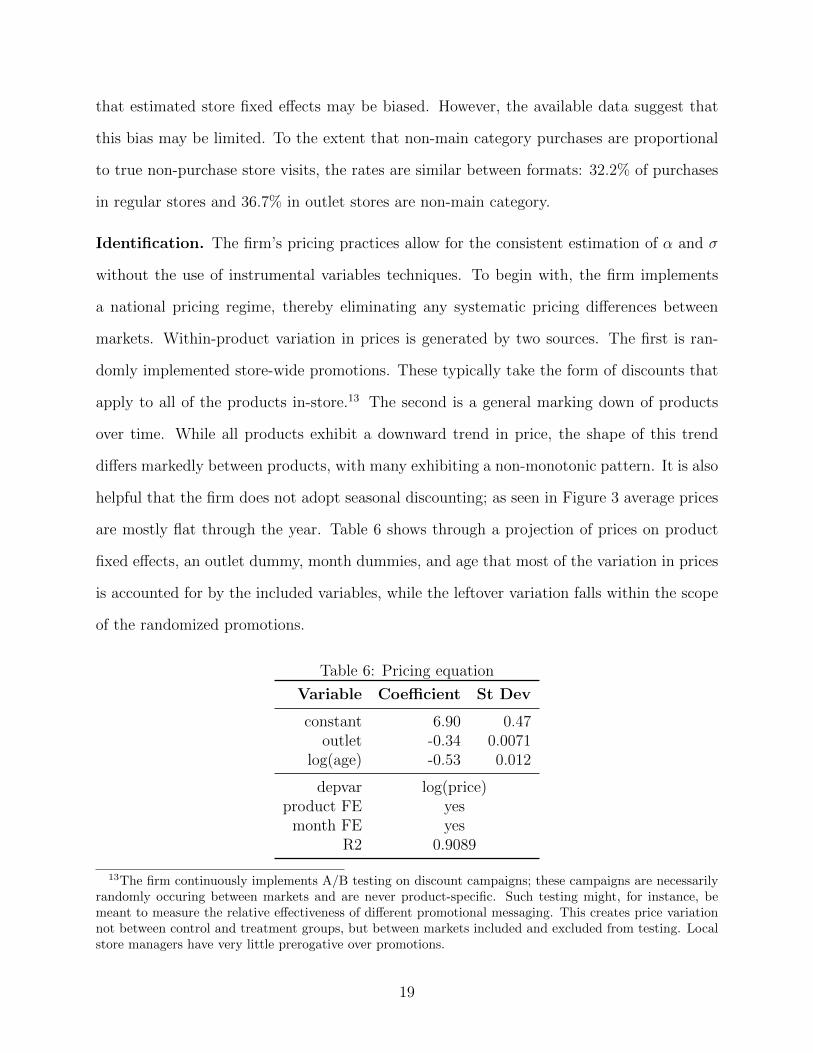
are mostly flat through the year. Table 6 shows through a projection of prices on product

fixed effects, an outlet dummy, month dummies, and age that most of the variation in prices

is accounted for by the included variables, while the leftover variation falls within the scope

of the randomized promotions.

Table 6: Pricing equation

Variable Coefficient St Dev

constant 6.90 0.47outlet -0.34 0.0071

log(age) -0.53 0.012

depvar log(price)product FE yes

month FE yesR2 0.9089

13The firm continuously implements A/B testing on discount campaigns; these campaigns are necessarilyrandomly occuring between markets and are never product-specific. Such testing might, for instance, bemeant to measure the relative effectiveness of different promotional messaging. This creates price variationnot between control and treatment groups, but between markets included and excluded from testing. Localstore managers have very little prerogative over promotions.

19

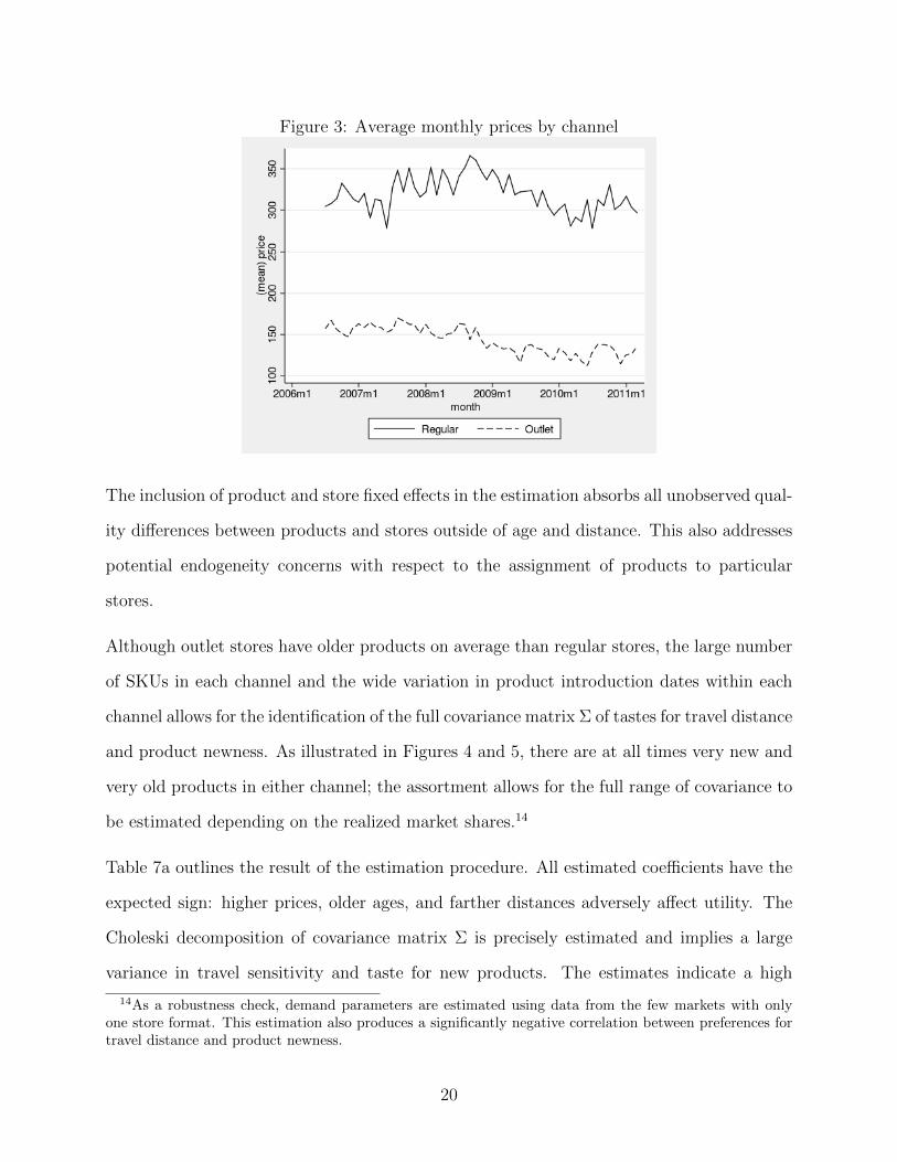
Figure 3: Average monthly prices by channel

The inclusion of product and store fixed effects in the estimation absorbs all unobserved qual-

ity differences between products and stores outside of age and distance. This also addresses

potential endogeneity concerns with respect to the assignment of products to particular

stores.

Although outlet stores have older products on average than regular stores, the large number

of SKUs in each channel and the wide variation in product introduction dates within each

channel allows for the identification of the full covariance matrix Σ of tastes for travel distance

and product newness. As illustrated in Figures 4 and 5, there are at all times very new and

very old products in either channel; the assortment allows for the full range of covariance to

be estimated depending on the realized market shares.14

Table 7a outlines the result of the estimation procedure. All estimated coefficients have the

expected sign: higher prices, older ages, and farther distances adversely affect utility. The

Choleski decomposition of covariance matrix Σ is precisely estimated and implies a large

variance in travel sensitivity and taste for new products. The estimates indicate a high

14As a robustness check, demand parameters are estimated using data from the few markets with onlyone store format. This estimation also produces a significantly negative correlation between preferences fortravel distance and product newness.

20

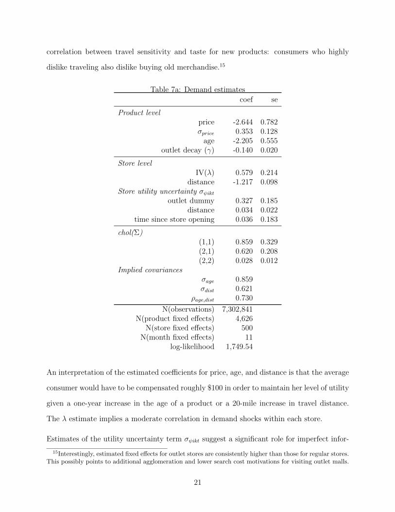
correlation between travel sensitivity and taste for new products: consumers who highly

dislike traveling also dislike buying old merchandise.15

Table 7a: Demand estimates

coef se

Product levelprice -2.644 0.782σprice 0.353 0.128

age -2.205 0.555outlet decay (γ) -0.140 0.020

Store levelIV(λ) 0.579 0.214

distance -1.217 0.098Store utility uncertainty σψikt

outlet dummy 0.327 0.185distance 0.034 0.022

time since store opening 0.036 0.183

chol(Σ)(1,1) 0.859 0.329(2,1) 0.620 0.208(2,2) 0.028 0.012

Implied covariancesσage 0.859σdist 0.621

ρage,dist 0.730

N(observations) 7,302,841N(product fixed effects) 4,626

N(store fixed effects) 500N(month fixed effects) 11

log-likelihood 1,749.54

An interpretation of the estimated coefficients for price, age, and distance is that the average

consumer would have to be compensated roughly $100 in order to maintain her level of utility

given a one-year increase in the age of a product or a 20-mile increase in travel distance.

The λ estimate implies a moderate correlation in demand shocks within each store.

Estimates of the utility uncertainty term σψikt suggest a significant role for imperfect infor-

15Interestingly, estimated fixed effects for outlet stores are consistently higher than those for regular stores.This possibly points to additional agglomeration and lower search cost motivations for visiting outlet malls.

21

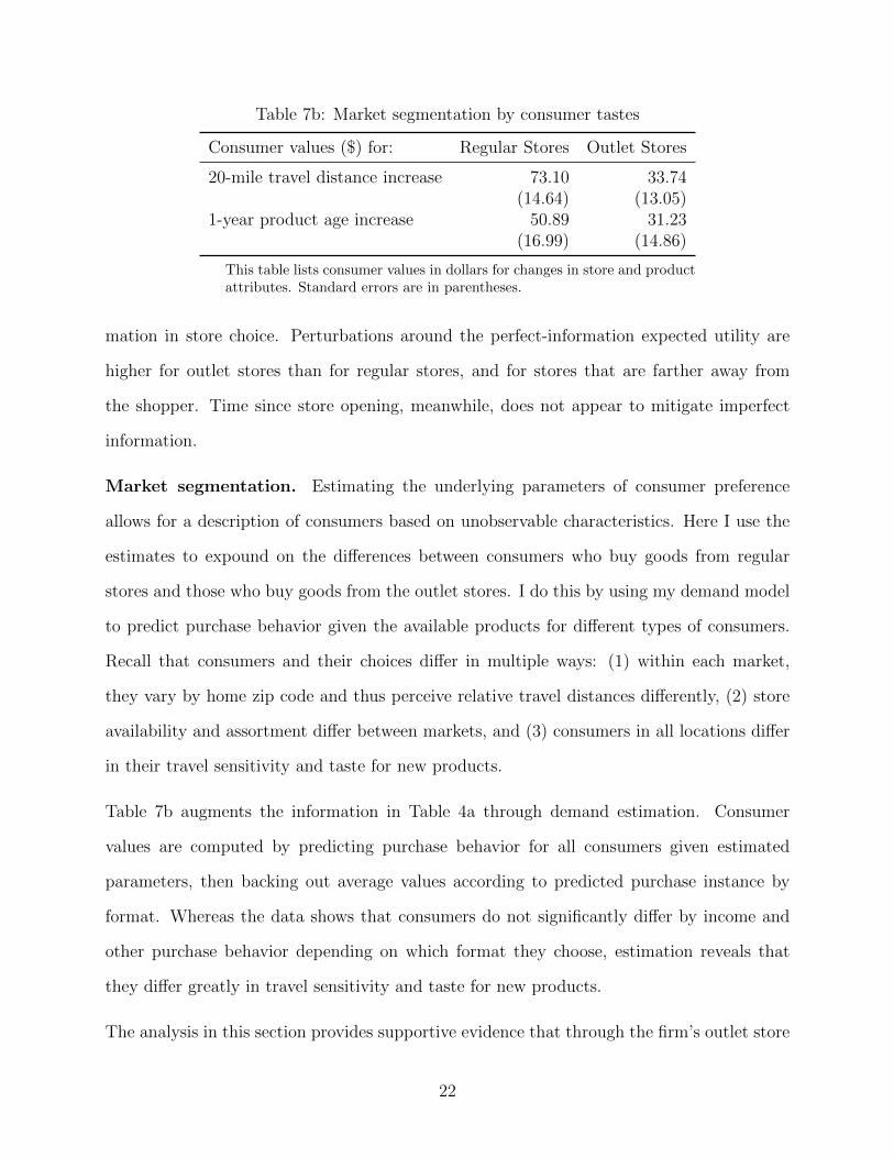
Table 7b: Market segmentation by consumer tastes

Consumer values ($) for: Regular Stores Outlet Stores

20-mile travel distance increase 73.10 33.74(14.64) (13.05)

1-year product age increase 50.89 31.23(16.99) (14.86)

This table lists consumer values in dollars for changes in store and productattributes. Standard errors are in parentheses.

mation in store choice. Perturbations around the perfect-information expected utility are

higher for outlet stores than for regular stores, and for stores that are farther away from

the shopper. Time since store opening, meanwhile, does not appear to mitigate imperfect

information.

Market segmentation. Estimating the underlying parameters of consumer preference

allows for a description of consumers based on unobservable characteristics. Here I use the

estimates to expound on the differences between consumers who buy goods from regular

stores and those who buy goods from the outlet stores. I do this by using my demand model

to predict purchase behavior given the available products for different types of consumers.

Recall that consumers and their choices differ in multiple ways: (1) within each market,

they vary by home zip code and thus perceive relative travel distances differently, (2) store

availability and assortment differ between markets, and (3) consumers in all locations differ

in their travel sensitivity and taste for new products.

Table 7b augments the information in Table 4a through demand estimation. Consumer

values are computed by predicting purchase behavior for all consumers given estimated

parameters, then backing out average values according to predicted purchase instance by

format. Whereas the data shows that consumers do not significantly differ by income and

other purchase behavior depending on which format they choose, estimation reveals that

they differ greatly in travel sensitivity and taste for new products.

The analysis in this section provides supportive evidence that through the firm’s outlet store

22

strategy, it segments consumers according to their underlying preferences for travel and

newness. Discounts in outlet stores seem deep enough to cater to lower-value consumers,

but not enough to cater to consumers who place a high premium on convenience and new

arrivals.

A complete argument for these conclusions requires studying counterfactual store configu-

rations and the associated consumer responses. The natural counterfactual scenario is one

in which the firm chooses not to open locations in outlet malls. It would be insufficient,

however, to simply remove these locations from the data and simulate purchase behavior.

The firm would presumably charge different prices in its regular stores in the absence of

outlet stores. Since outlet stores form an integral part of the firm’s distribution strategy,

removing them would also motivate changes in the how the firm stocks its regular stores.

The following section provides a framework for thinking about how the firm chooses prices

and product assortments given its dual distribution strategy. The purpose of modeling

supply is to form a basis, together with the demand model, for predicting firm performance

given a counterfactual distribution strategy.

6 Supply

In this section I develop a model of firm behavior with respect to price-setting and product

assortment choice. This model permits a careful comparison of firm performance under

counterfactual consumer characteristics and alternative distribution strategies, and hence

sheds light on the profitability of outlet stores. This also allows an examination of the firm’s

costs, which serve as both a basis for the policy simulations and an indicator of the validity

of the model’s assumptions.

Two major assumptions are maintained throughout this section. The first is that the firm be-

haves like a monopolist, setting prices and product characteristics without strategic consider-

23

ations. The second is that the firm’s prices and product choices maximize profits conditional

on store locations. I discuss each of these assumptions before describing the model.

The monopoly assumption is motivated by the firm’s unique position in the industry. It has

a 30-40 percent share of total industry revenues, and an even larger share in its particular

psychographic segment. The next largest brand accounts for about 10 percent of industry

revenues. Their products, however, retail at about the $1,000 price point—much higher

than the data provider’s average price of $300. There is arguably little overlap between the

market for the data provider’s products and the market for higher-end products such as

those carried by the number two brand.16

The firm’s dominant position also motivates the assumption that the firm is profit-maximizing.

There may be very few firms for which this is a more appropriate assumption to make, given

the firm’s reputation not only in its category but also across industries. The firm consistently

ranks among the top 10 firms across all industries in revenue per square foot of retail space,

which is a standard performance metric among retailers.

I categorize firm decisions according to long- and short-term horizons. Long-term decisions

concern store locations, stylistic product characteristics, and store capacities. Short-term

decisions consist of pricing and the choice of product introduction rates. In my supply

model, I take the firm’s long-term decisions as exogenous, and treat the short-term decisions

as endogenous.

I now proceed to describe the supply model in detail. First I discuss pricing. The monopoly

pricing assumption, combined with the previous section’s demand model, implies marginal

costs for each product. I show how these marginal costs relate to observed product char-

acteristics. Next I add endogenous product choice. The added features, combined with the

pricing and demand models, pin down product development costs.

16There is little publicly available information with more precise figures; however, these market shares areconfirmed by the firm’s managers. They also agree with the notion that competitors’ pricing trends havelittle or no impact on the firm’s pricing decisions.

24

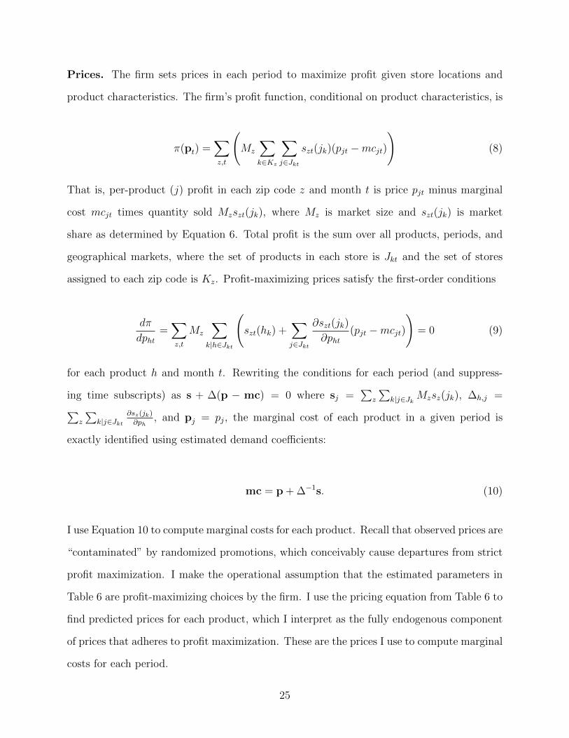
Prices. The firm sets prices in each period to maximize profit given store locations and

product characteristics. The firm’s profit function, conditional on product characteristics, is

π(pt) =∑z,t

(Mz

∑k∈Kz

∑j∈Jkt

szt(jk)(pjt −mcjt)

)(8)

That is, per-product (j) profit in each zip code z and month t is price pjt minus marginal

cost mcjt times quantity sold Mzszt(jk), where Mz is market size and szt(jk) is market

share as determined by Equation 6. Total profit is the sum over all products, periods, and

geographical markets, where the set of products in each store is Jkt and the set of stores

assigned to each zip code is Kz. Profit-maximizing prices satisfy the first-order conditions

dπ

dpht=∑z,t

Mz

∑k|h∈Jkt

(szt(hk) +

∑j∈Jkt

∂szt(jk)

∂pht(pjt −mcjt)

)= 0 (9)

for each product h and month t. Rewriting the conditions for each period (and suppress-

ing time subscripts) as s + ∆(p − mc) = 0 where sj =∑

z

∑k|j∈Jk Mzsz(jk), ∆h,j =∑

z

∑k|j∈Jkt

∂sz(jk)∂ph

, and pj = pj, the marginal cost of each product in a given period is

exactly identified using estimated demand coefficients:

mc = p + ∆−1s. (10)

I use Equation 10 to compute marginal costs for each product. Recall that observed prices are

“contaminated” by randomized promotions, which conceivably cause departures from strict

profit maximization. I make the operational assumption that the estimated parameters in

Table 6 are profit-maximizing choices by the firm. I use the pricing equation from Table 6 to

find predicted prices for each product, which I interpret as the fully endogenous component

of prices that adheres to profit maximization. These are the prices I use to compute marginal

costs for each period.

25

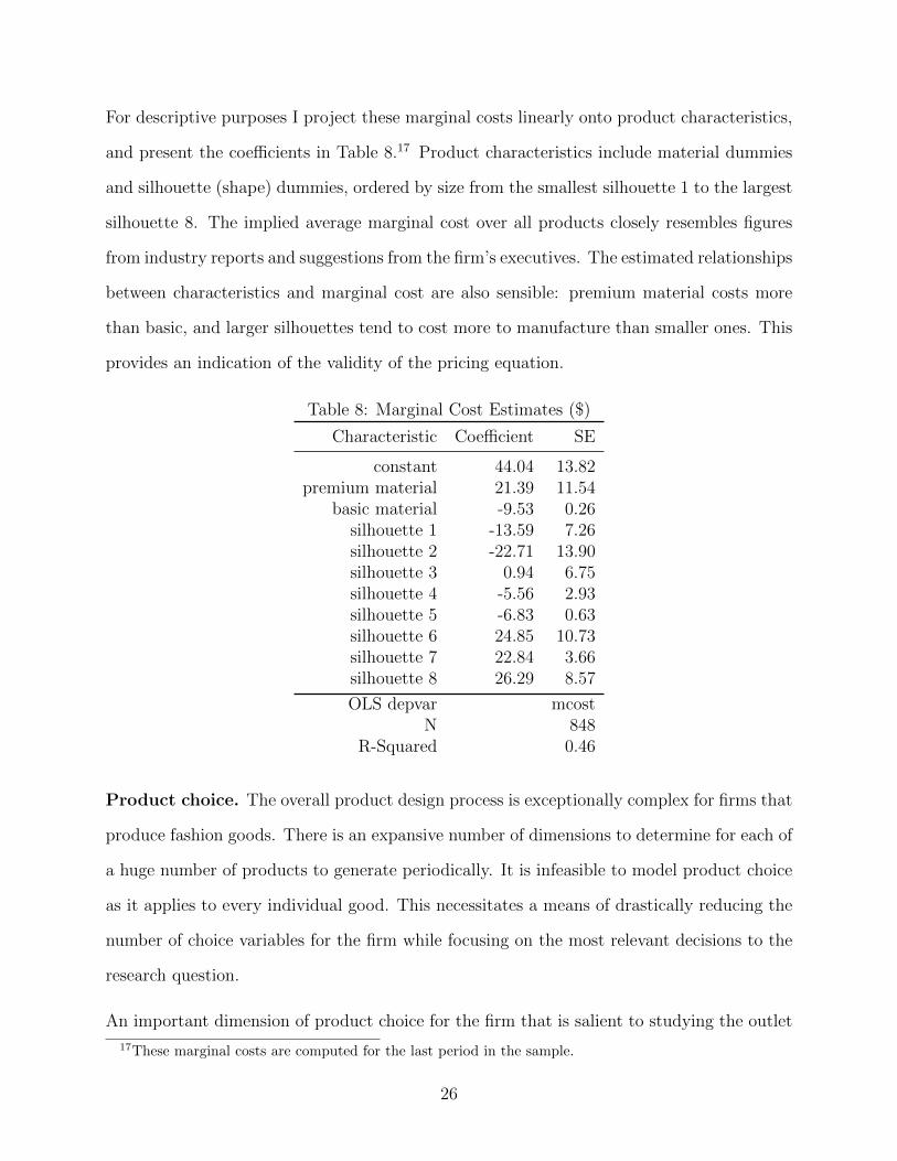
For descriptive purposes I project these marginal costs linearly onto product characteristics,

and present the coefficients in Table 8.17 Product characteristics include material dummies

and silhouette (shape) dummies, ordered by size from the smallest silhouette 1 to the largest

silhouette 8. The implied average marginal cost over all products closely resembles figures

from industry reports and suggestions from the firm’s executives. The estimated relationships

between characteristics and marginal cost are also sensible: premium material costs more

than basic, and larger silhouettes tend to cost more to manufacture than smaller ones. This

provides an indication of the validity of the pricing equation.

Table 8: Marginal Cost Estimates ($)

Characteristic Coefficient SE

constant 44.04 13.82premium material 21.39 11.54

basic material -9.53 0.26silhouette 1 -13.59 7.26silhouette 2 -22.71 13.90silhouette 3 0.94 6.75silhouette 4 -5.56 2.93silhouette 5 -6.83 0.63silhouette 6 24.85 10.73silhouette 7 22.84 3.66silhouette 8 26.29 8.57

OLS depvar mcostN 848

R-Squared 0.46

Product choice. The overall product design process is exceptionally complex for firms that

produce fashion goods. There is an expansive number of dimensions to determine for each of

a huge number of products to generate periodically. It is infeasible to model product choice

as it applies to every individual good. This necessitates a means of drastically reducing the

number of choice variables for the firm while focusing on the most relevant decisions to the

research question.

An important dimension of product choice for the firm that is salient to studying the outlet

17These marginal costs are computed for the last period in the sample.

26

store strategy is that of product lifespans in each format. By lifespan, I mean the amount

of time a product is available for purchase in each format. Figure 2 shows how product

lifespans are determined by the flow of inventory into, between, and out of store formats.

New products flow into both formats when “original” and “factory” products are born (see

Table 3). All products in the regular store are eventually transferred to the outlet store,

where the last units of each style is sold.

One advantage of using the current dataset to study firm product choice is that the outlet

store strategy provides a structure that delimits the firm’s choice set. The technology that

the firm uses to create product age-distance combinations—physically transferring prod-

ucts between formats—is completely transparent and can mostly be considered cost-neutral.

This is in contrast to most other cases, where both product assembly technologies and cost

structures are more complex.

Although the number of new products in each format can conceivably be modeled using

existing techniques, the selection of which products to transfer or discontinue presents a

different challenge. Because the firm offers such a large number of products, an attractive

option is to think of the firm as targeting a joint probability of product characteristics rather

than individual product attributes. A primary contribution of this paper is a demonstration

of this novel approach to modeling multidimensional product differentiation.

Specifically, I assume that store locations and capacities are given. Let Ck be the number

of items that store k can display on its shelves. I assume that in each period, each store

k of format fmt ∈ {regular, outlet} takes Ck draws from the corresponding master set of

products, described by the distribution of product characteristics φfmt. Let φfmt = ffmt ×

gfmt, where ffmt is the distribution of endogenous product characteristics (product ages in

this setting) and gfmt governs the exogenous characteristics (summarized here by ξj).18 The

firm’s objective is to choose the profit-maximizing shapes of fregular and foutlet.

18Treating ξj as exogenous can be rationalized by the fact that the firm usually cannot ascertain the appealof a product to consumers before it is taken to market.

27

In order to make this problem tractable, I propose to construct ffmt using a set of parametric

distributions. Industry logistics and the data suggest a natural choice for these distributions

and a direct interpretation of their parameters. Consider these assumptions on product

assortment:

1. Original products in the regular format have an average probability x of being trans-

ferred to the outlet format in the next period

2. Factory products in the outlet format have an average probability y of being retired in

the next period

3. Original products in the outlet format have an average probability z of being retired

in the next period

4. Factory goods make up a proportion α of goods in the outlet format

These assumptions imply that if X is product age in the regular format and Y is product

age in the outlet format then

X ∼ Geometric(x) (11)

Y =

W with probability α

X + Z with probability 1− α(12)

where W ∼ Geometric(y) and Z ∼ Geometric(z)

By adjusting the stopping probabilities x, y, and z, the firm can control the relative distri-

butions of product age in each store format. These probabilities also pin down the portion of

products that are new introductions in each period: the share of original products that are

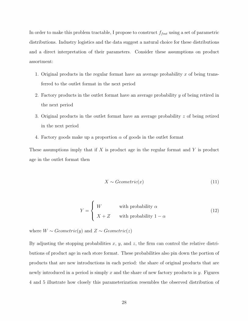
newly introduced in a period is simply x and the share of new factory products is y. Figures

4 and 5 illustrate how closely this parameterization resembles the observed distribution of

28

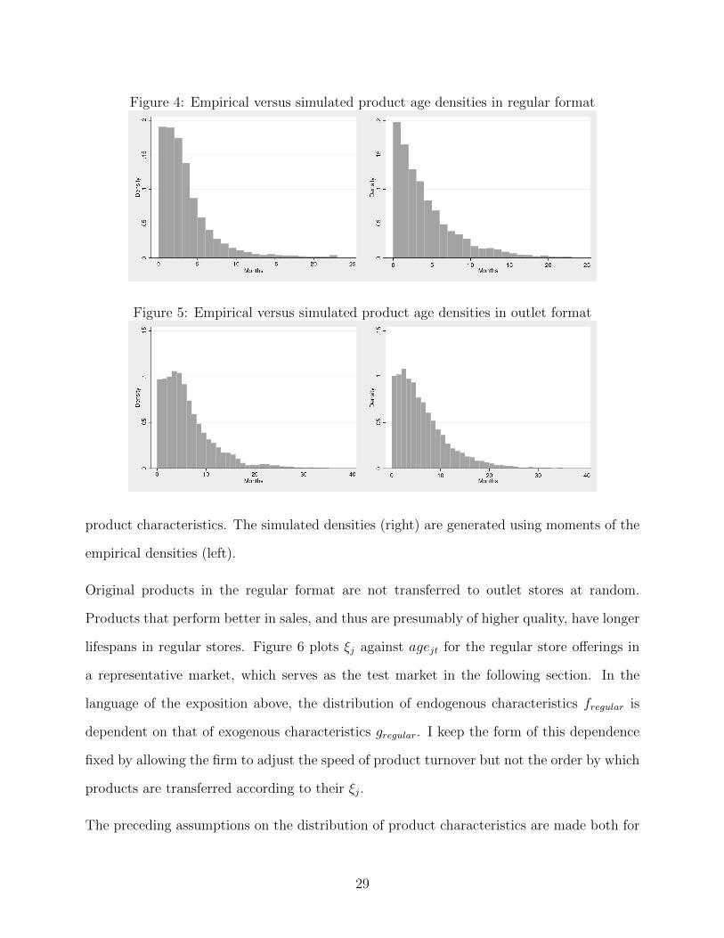
Figure 4: Empirical versus simulated product age densities in regular format

Figure 5: Empirical versus simulated product age densities in outlet format

product characteristics. The simulated densities (right) are generated using moments of the

empirical densities (left).

Original products in the regular format are not transferred to outlet stores at random.

Products that perform better in sales, and thus are presumably of higher quality, have longer

lifespans in regular stores. Figure 6 plots ξj against agejt for the regular store offerings in

a representative market, which serves as the test market in the following section. In the

language of the exposition above, the distribution of endogenous characteristics fregular is

dependent on that of exogenous characteristics gregular. I keep the form of this dependence

fixed by allowing the firm to adjust the speed of product turnover but not the order by which

products are transferred according to their ξj.

The preceding assumptions on the distribution of product characteristics are made both for

29

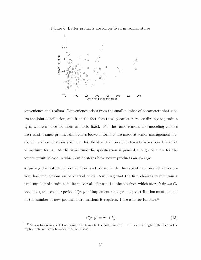
Figure 6: Better products are longer-lived in regular stores

convenience and realism. Convenience arises from the small number of parameters that gov-

ern the joint distribution, and from the fact that these parameters relate directly to product

ages, whereas store locations are held fixed. For the same reasons the modeling choices

are realistic, since product differences between formats are made at senior management lev-

els, while store locations are much less flexible than product characteristics over the short

to medium terms. At the same time the specification is general enough to allow for the

counterintuitive case in which outlet stores have newer products on average.

Adjusting the restocking probabilities, and consequently the rate of new product introduc-

tion, has implications on per-period costs. Assuming that the firm chooses to maintain a

fixed number of products in its universal offer set (i.e. the set from which store k draws Ck

products), the cost per period C(x, y) of implementing a given age distribution must depend

on the number of new product introductions it requires. I use a linear function19

C(x, y) = ax+ by (13)

19As a robustness check I add quadratic terms to the cost function. I find no meaningful difference in theimplied relative costs between product classes.

30

to represent these costs.

I assume that the firm chooses product choice parameters x, y, z, and α once to maximize

expected profit

E(π|x, y, z, α,pt) =∑fmt

∫ ∑z,t

Mz

∑k

∑j∈Jkt

szt(jk)(pjt −mcjt)dffmt(x, y, z, α)−C(x, y) (14)

where pt is a vector of optimal prices for any realization of product characteristics.

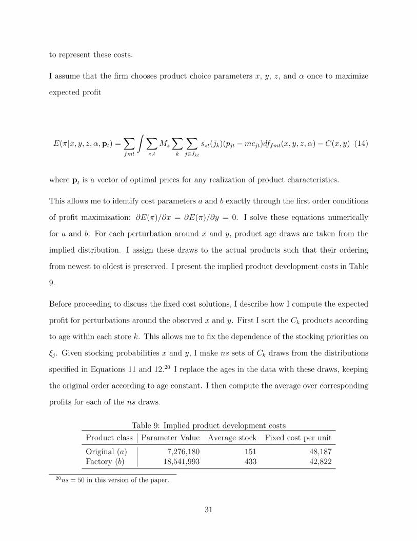
This allows me to identify cost parameters a and b exactly through the first order conditions

of profit maximization: ∂E(π)/∂x = ∂E(π)/∂y = 0. I solve these equations numerically

for a and b. For each perturbation around x and y, product age draws are taken from the

implied distribution. I assign these draws to the actual products such that their ordering

from newest to oldest is preserved. I present the implied product development costs in Table

9.

Before proceeding to discuss the fixed cost solutions, I describe how I compute the expected

profit for perturbations around the observed x and y. First I sort the Ck products according

to age within each store k. This allows me to fix the dependence of the stocking priorities on

ξj. Given stocking probabilities x and y, I make ns sets of Ck draws from the distributions

specified in Equations 11 and 12.20 I replace the ages in the data with these draws, keeping

the original order according to age constant. I then compute the average over corresponding

profits for each of the ns draws.

Table 9: Implied product development costs

Product class Parameter Value Average stock Fixed cost per unit

Original (a) 7,276,180 151 48,187Factory (b) 18,541,993 433 42,822

20ns = 50 in this version of the paper.

31

The parameter values in Table 9 indicate the cost of replacing the entire stock of products,

i.e., when x = 1 or y = 1.21 Dividing these values by the average stock of each class

of product gives the fixed costs associated with developing each unit.22 “Original” and

“factory” products in Table 9 refer to product types and not to different formats, hence

dividing by the average stock of each product type is consistent with the supply model.

Although there are more original designs produced per period, there is more space allotted

for factory products at outlet stores. Hence b > a since it would cost the firm more to replace

the entire stock every period. I find that producing each style of product carries a fixed cost

of about $50,000, and that the fixed cost of producing an original product is significantly

higher than the fixed cost of a factory product.

With the model of price-setting and product introduction discussed in this section, together

with the fixed and marginal costs that they imply, counterfactual store configurations can

now be properly evaluated.

7 Policy Simulations

The basic question that this paper addresses is: Why do outlet stores exist? In this section,

I explore this question by simulating situations in which the firm pursues selling strategies

that exclude some aspect of outlet store retail. For each of these policy simulations, I use the

supply-side model in Section 6 to predict how the firm would change its pricing and product

introduction rates in response to changes in other store attributes. The demand model from

Section 5 then shows how consumers would react to these changes. Specifically, I simulate

four scenarios: the removal of outlet stores, random assortment of styles between regular

and outlet stores, relocating outlet stores to city centers, and improvements in outlet store

service and promotion. I find that outlet stores serve to expand the firm’s market to include

21The empirical values of x and y are 0.19 and 0.09, respectively22The average stock is defined as the average number of styles in the entire product universe (across all

stores) observed in a month.

32

consumers who are more sensitive to prices, less averse to travel, and less particular about

product ages. Furthermore, the assortment in outlet stores is chosen to prevent higher-value

consumers from preferring to visit outlet stores over regular stores.

Test market. In order to clearly demonstrate the effects of each experiment, I use a

representative market over which to perform policy simulations. The test market is the

Indianapolis-Carmel Metropolitan Statistical Area in July 2007.23 This market is represen-

tative of the firm’s markets both in terms of the demand profile and the firm’s store and

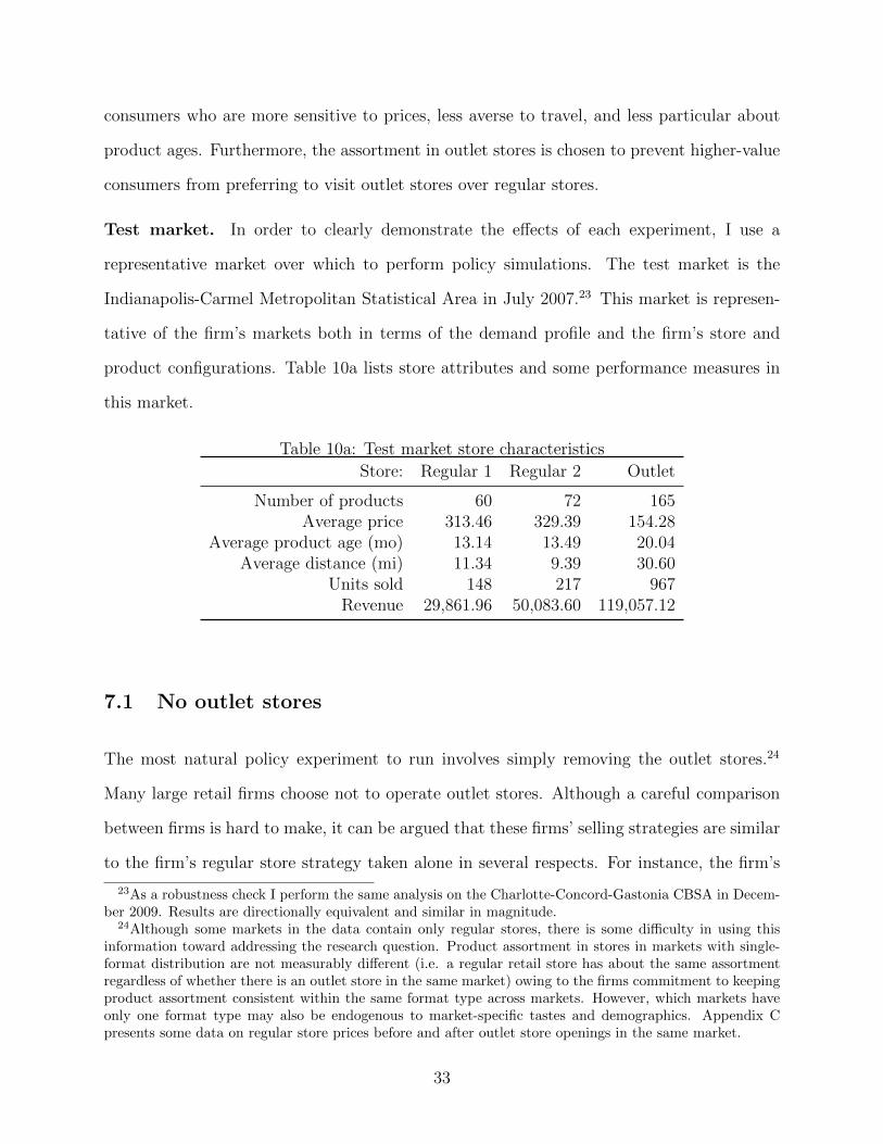
product configurations. Table 10a lists store attributes and some performance measures in

this market.

Table 10a: Test market store characteristics

Store: Regular 1 Regular 2 Outlet

Number of products 60 72 165Average price 313.46 329.39 154.28

Average product age (mo) 13.14 13.49 20.04Average distance (mi) 11.34 9.39 30.60

Units sold 148 217 967Revenue 29,861.96 50,083.60 119,057.12

7.1 No outlet stores

The most natural policy experiment to run involves simply removing the outlet stores.24

Many large retail firms choose not to operate outlet stores. Although a careful comparison

between firms is hard to make, it can be argued that these firms’ selling strategies are similar

to the firm’s regular store strategy taken alone in several respects. For instance, the firm’s

23As a robustness check I perform the same analysis on the Charlotte-Concord-Gastonia CBSA in Decem-ber 2009. Results are directionally equivalent and similar in magnitude.

24Although some markets in the data contain only regular stores, there is some difficulty in using thisinformation toward addressing the research question. Product assortment in stores in markets with single-format distribution are not measurably different (i.e. a regular retail store has about the same assortmentregardless of whether there is an outlet store in the same market) owing to the firms commitment to keepingproduct assortment consistent within the same format type across markets. However, which markets haveonly one format type may also be endogenous to market-specific tastes and demographics. Appendix Cpresents some data on regular store prices before and after outlet store openings in the same market.

33

regular stores are of similar size, configuration, and location to those of a competitor, even

though the competitor does not sell through outlet stores.

Columns 1a to 1c of Table 10b contain the results of this counterfactual as they pertain to

the supply- and demand-side responses. Column 1a shows that revenues in regular stores

increase compared to the baseline when the outlet store is closed, even when prices and

assortment in the regular stores remain the same. Column 1b shows that the firm would

lower prices in regular stores in the absence of outlet stores, even if it could not change the

assortment (see Appendix B for details on finding optimal prices). Column 1c shows that

the firm would choose to make fewer product introductions if outlet stores did not exist,

resulting in an increase in average product age in these stores.

The story is rounded out by looking at details of the demand-side response. Closing the

outlet store initially results in a very small increase in regular store revenues because few

of the consumers who shopped at the outlet store switch to regular stores. When allowed

to change product characteristics, the firm lowers quality and price in the regular stores to

cater to the lower-value consumers. However, even given this flexibility, the firm is unable

to serve the full range of consumers that it can with the outlet stores present.

An important caveat to this analysis is that brand image effects are not modeled.25 Removing

outlet stores in the overall market may enhance the brand’s overall image among certain

clients, mitigating the negative results found here. In addition Qian et al. (2013) find

that outlet stores can have positive brand awareness effects in both channels. The case

considered in Section 7.3, in which the outlet store is maintained but transferred to the city

center, provides a setting that is less prone to these concerns.

25In an effort to detect such effects I compared the estimated store fixed effects for regular stores in marketswith and without outlet stores; however no meaningful systematic difference exists.

34

7.2 Random assortment

The assignment of products to either regular stores or outlet stores forms an important

part of the firm’s selling strategy. In this subsection, I show the value of the firm’s ob-

served assortment strategy by comparing its observed performance with that achieved by

a counterfactual assortment strategy in which products are randomly assigned to stores.

This random assignment results in a configuration in which regular and outlet stores contain

roughly identical assortments.26,27 This counterfactual strategy resembles that of firms that

open stores in outlet malls, but do not distinguish the assortment in these stores from those

in their non-outlet locations.

Column 2a in Table 10b describes the resulting average product characteristics in these stores.

Here I allow the firm to adjust prices, so that in both cases prices are profit-maximizing,

conditional on product assortments. Jumbling the products results in near-identical average

product qualities between stores, but prices are still much lower in the outlet store. This

suggests that the bulk of discounting in outlet stores is to compensate for the inconvenience

associated with longer travel times.

The firm’s performance suffers under a random assignment of products to stores. Revenues

in all stores decrease, and consumers are less different between formats. This should be

unsurprising, given that the products are less different between formats. My hypothesis is

that sorting works exceptionally well because there is a positive correlation between consumer

travel sensitivity and taste for newness. To test this hypothesis, I run the same counterfactual

but under a supposed form of consumer heterogeneity in which there is zero correlation

between travel sensitivity and tastes for newness.

Columns 2b and 2c in Table 10b has the results of this experiment. As anticipated, ran-

domizing assortment has less of an effect when consumer tastes for the two attributes are

26Recall that a product is unique only up to its fixed effect ξj , its price pj , and its vintage agej .27Outlet stores will still have more shelf space than regular stores.

35

uncorrelated. There was little sorting to begin with, so the decrease does not come with very

big a cost. Optimal prices between the two formats approach each other as the assortment

becomes more similar.

7.3 Centrally-located outlet stores

One viewpoint is that the firm implements a “damaged goods” strategy by selling a portion

of its goods in distant locations. In order to consider this hypothesis, I run a third set of

counterfactuals in which outlet stores are moved to central locations. I show that (i) revenues

decrease, (ii) the firm would make fewer product introductions in the outlet format, and (iii)

it would cater to a narrower range of consumers.

An alternative explanation to damaged goods is that firms locate in outlet malls to take

advantage of lower rents. Outlet malls on average set a monthly rent of $29.76 per square

foot, which can be dwarfed by rents in the most prestigious retail locations (Humphers, 2012).

However, this rent is close to the average for retail space in many urban centers—implying

that the firm could choose to costlessly relocate its outlet stores closer to its target market.

These locations may not be as attractive and brand-consistent as the more expensive areas

of the city, but neither are the areas in which most outlet malls are located.

Column 3 of Table 10b presents the results of the experiment in which the outlet store is

moved into the central shopping district. Notably, while prices are less variable now (regular

store products are cheaper and outlet store products are more expensive), quality along the

age dimension is more variable (regular store products are slightly newer and outlet store

products are much older). Denied the ability to differentiate products according to location,

the firm increases the level of differentiation according to age. The range of consumers that

the firm is able to reach, nevertheless, is similar to the case in which the outlet store is simply

shut down.

36

7.4 Improved outlet stores

Outlet stores differ from regular stores in more ways than just location and product assort-

ment. They receive less promotional support, are typically less attractively designed, and

offer lower service levels. For these reasons shopping at an outlet store may offer lower utility

apart from that caused by a less desirable assortment. The demand side of the model used

in this paper accounts for these differences by allowing outlet stores to have negative format

effects on perceived product quality, and a lower awareness among shoppers of the product

assortment. In the following pair of counterfactuals I investigate the potential benefits to

the firm of improving outlet stores along these dimensions. In particular I set the outlet

adjustment γ on perceived original product quality and the outlet component of imperfect

information shocks ψik to zero and predict firm and consumer reactions. Columns 4a and

4b in Table 10b present the supply-side responses and outcomes.

Both improvements to the outlet store experience result in higher revenues and profits. In

column 4a, the firm adjusts by increasing the product age difference but decreasing the

price differential between formats. The intuition is that removing the outlet store multiplier

diminishes the quality differences between formats and therefore the firm compensates by

adjusting the product age difference. Because consumers are heterogeneous in their taste

for product newness but not in the intrinsic quality (fixed effects) of the products, the

price difference can be relaxed in favor of higher revenues without the danger of excess

cannibalization.

In column 4b, increased consumer certainty about outlet store utility also improves firm per-

formance, even though optimal prices and product ages are similar to the baseline. The rea-

son is that consumers who receive negative shocks disproportionately opt for non-purchase,

while consumers who receive positive shocks disproportionately trade down from visiting the

regular store. While variable profits improve in both of the cases considered, it is possible

that the level of investment required to implement such improvements may prove too high to

37

justify. However, it is clear that in the management of outlet stores service and promotion

effects are nontrivial relative that that of product assortment and pricing.

This section’s counterfactuals show that adopting outlet stores helps the firm in many ways.

It extends the firm’s market to include consumers who are not averse to traveling and less

desirous of new products. Since these are the same people in the data, it makes sense for

the firm to populate its outlet stores with older products. This has the additional benefit

of making outlet store products less attractive to higher-value consumers, thus preventing

cannibalization.

8 Conclusion

Owning and operating outlet stores constitutes a major component of many firms’ distri-

bution strategies, particularly in the clothing and fashion industries. It is an interesting

practice that continues to evolve and gain popularity. Yet there has been little written in

the marketing and economics literatures that speaks to the reasons for the success of outlet

stores, or the mechanisms by which they improve firm performance. The availability of new

sales data from a major fashion goods manufacturer and retailer offers a unique opportunity

to empirically investigate how outlet stores work.

This paper shows that outlet stores provide several benefits as a tool of price discrimination.

Outlet stores allow the firm to serve lower-value consumers without lowering prices faced by

its regular store clientele. By stocking outlet stores with less desirable products, the firm

exploits the positive correlation between consumers’ travel sensitivity and taste for quality.

Prices are low in outlet stores, but not low enough to attract consumers who value quality

and convenience the most.

The model of product choice in this paper suggests a benefit of running outlet stores apart

from its price discrimination uses: it allows the firm to make more frequent new product

38

Tab

le10

b:

Res

ult

sof

counte

rfac

tual

sim

ula

tion

s

Bas

elin

eN

oou

tlet

store

Ran

dom

ass

ort

men

tC

entr

al

Imp

rove

men

ts1a

1b

1c

2a

2b

2c

34a

4b

SU

PP

LY

Regular1

Pri

ce31

3.46

313.4

6278.7

3218.2

7297.2

3277.3

2274.8

3309.8

4309.5

2332.8

2A

ge13

.14

13.1

413.1

415.5

616.9

213.1

416.9

212.2

413.0

213.1

2R

even

ue

29,8

6233

,254

36,9

90

37,3

84

25,8

58

22,7

42

22,6

82

21,1

13

30,8

53

31,8

42

Regular2

Pri

ce32

9.39

329.3

9301.0

0250.0

3300.1

3282.9

8279.7

8312.3

8312.6

4346.0

1A

ge13

.49

13.4

913.4

915.5

617.4

313.4

917.4

312.5

713.2

213.4

2R

even

ue

50,0

8457

,101

64,8

57

69,3

86

43,2

15

37,2

11

36,8

49

38,8

96

51,4

89

52,3

66

Outlet

Pri

ce15

4.28

172.9

6150.0

7163.7

5202.1

6165.3

9157.2

7A

ge20

.04

17.1

820.0

417.1

824.3

022.8

220.0

3R

even

ue

119,

057

103,5

09

95,0

44

93,3

90

101,8

50

125,1

18

119,0

10

Tot

alre

venu

e19

9,00

390

,355

101,8

47

106,7

70

172,5

82

154,9

97

152,9

21

161,8

59

207,4

60

202,8

58

Var

iab

lep

rofi

t10

6,72

862

,347

75,3

67

82,2

13

83,6

58

75,3

24

73,0

98

70,1

83

114,1

03

115,6

29

DE

MA

ND

Regular1

Dis

tan

ceav

ersi

on75

.78

71.5

566.8

965.3

972.1

355.1

554.7

867.3

175.7

975.6

6A

geav

ersi

on44

.91

42.2

138.9

234.8

341.1

340.0

239.0

835.9

246.5

544.8

6Regular2

Dis

tan

ceav

ersi

on83

.62

82.7

574.2

372.1

778.3

763.6

961.8

474.1

883.9

283.4

3A

geav

ersi

on42

.12

41.0

536.6

832.4

238.9

636.1

936.2

333.9

843.7

841.8

7Outlet

Dis

tan

ceav

ersi

on35

.94

42.0

843.6

044.6

456.7

335.7

337.9

3A

geav

ersi

on24

.44

36.8

731.9

233.4

728.5

923.3

425.5

6

Note

s:C

on

sum

ervalu

esp

rese

nte

das

dem

an

dre

sult

sare

aver

ages

over

each

store

.D

ista

nce

aver

sion

isth

ed

ollar

equ

ivale

nt

of

a20-m

ile

incr

ease

intr

avel

dis

tan

ce.

Age

aver

sion

iseq

uiv

ale

nt

toa

1-y

ear

incr

ease

inp

rod

uct

age.

Colu

mn

sd

enote

case

sin

wh

ich

:1a

-T

he

ou

tlet

store

iscl

ose

dan

dp

rice

san

dp

rod

uct

ages

inth

ere

gu

lar

store

sare

un

chan

ged

.1b

-T

he

ou

tlet

store

iscl

ose

dan

dp

rice

sin

the

regu

lar

store

sare

reop

tim

ized

1c

-T

he

ou

tlet

store

iscl

ose

dan

dp

rice

san

dp

rod

uct

ages

inth

ere

gu

lar

store

sare

reop

tim

ized

.2a

-P

rod

uct

sare

ran

dom

lyass

ign

edan

dp

rice

sare

reop

tim

ized

.2b

-D

eman

dsi

de

corr

elati

on

bet

wee

np

rod

uct

age

an

dtr

avel

sen

siti

vit

yis

set

toze

ro;

pri

ces

are

reop

tim

ized

.2c

-D

eman

dsi

de

corr

elati

on

bet

wee

np

rod

uct

age

an

dtr

avel

sen

siti

vit

yis

set

toze

ro;

pro

du

cts

are

ran

dom

lyass

ign

edan

dp

rice

sare

reop

tim

ized

.3

-T

he

ou

tlet

store

ism

oved

toth

eci

tyce

nte

r.4a

-O

utl

etst

ore

mu

ltip

lier

on

ori

gin

al

pro

du

ctfi

xed

effec

tsis

set

toze

ro.

4b

-O

utl

etst

ore

effec

ton

store

uti

lity

un

cert

ain

tyis

set

toze

ro.

39

introductions in its regular format. The firm offers more new products every period in its

regular stores both to increase the attractiveness of regular store offerings relative to those in

outlet stores and because it stocks outlet stores with older, less attractive products from the

regular stores. This can conceivably counter the threat that is most associated with outlet

stores: that it results in the dilution of prestige brands. Outlet stores may actually enable

the firm to improve its regular store products, which typically form the basis of a fashion

brand’s image.

Lessons from outlet store retail have wide applicability to questions of product line design

and price discrimination. Outlet stores are a specific response to the apparent heterogeneity

in tastes for quality and convenience among fashion shoppers. Similar responses by firms to

consumer tastes can be observed in the electronics and travel industries. The notion that

the correlation of characteristics in a firm’s product space ought to resemble the correlation

of consumer tastes for them may be useful to many firms.

The key insight is that multidimensionality in consumer preference heterogeneity matters

for product line design. Firms that seek to optimize their product offerings must take

into account how tastes vary for different product characteristics, and what the correlations

between those tastes are. This is not a new discovery: the existing theoretical literature on

multidimensional screening emphasizes the sensitivity of the optimal allocation set by the

principal to the agent’s value correlations. This is, however, the first demonstration of its

importance in an actual business setting. The choice of whether to operate outlet stores

hinges on a market landscape in which consumers who are most willing to travel to outlet

malls value quality the least.

While the static framework adopted in this paper is sufficient for the specific research ques-

tions, it does impose limitations on aspects of firm and consumer behavior that can be

incorporated. Some consumers may, for instance, forego the purchase of a particular original

product in the hope of eventually finding it in the outlet store. The firm may correspondingly

40

adopt strategies to induce uncertainty around the availability of original goods in the outlet

store. A fully specified dynamic model is needed to incorporate such interactions.

Another limitation arises from the focus of this work on specific product and store charac-

teristics. There are other unobserved aspects of outlet stores that are potentially relevant,

e.g. service levels, subjective product evaluations, and experiential factors—some of which

have been studied in previous work (e.g. Coughlan and Soberman 2005). There may also be

scope for firms to optimize over dimensions of product assortment apart from product age.

Accounting for these strategic choices may attenuate the losses measured in the counterfac-

tual simulations in Section 7. Given the diversity in selling strategies even among firms that

operate outlet stores, there is likely to be much variation in the relevance of each of these

factors between different cases.

There are many possible directions for future research. Outlet stores constitute a single

aspect of a consolidated selling strategy that has become standard among fashion goods

firms. Other parts of this strategy include price skimming, targeted coupons, and loyalty

programs. Many of these components operate on the intertemporal dimension of durable

goods demand. It would be interesting to see how they build on the firm’s overall product

lining strategy by adding yet additional dimensions.

This setting is also a prime vehicle for exploring alternative theories of consumer behavior

with respect to fashion goods demand. Consumers, for instance, may conceivably choose

products based on their capacity to signal status. Meanwhile, fashion goods may have

characteristics that are discernible to some consumers but not others (for instance, whether

a product is sold exclusively in outlet stores). This presents a unique product design challenge

to firms that wish to exploit these consumer preferences.

41

References

Armstrong, M. (1996). Multiproduct nonlinear pricing. Econometrica, pages 51–75.

Armstrong, M. and Rochet, J.-C. (1999). Multi-dimensional screening: A user’s guide.

European Economic Review, 43:959–979.

Bayus, B. L. and Putsis, W. P. (1999). Product proliferation: An empirical analysis of

product line determinants and market outcomes. Marketing Science, 18.2:137–153.

Bell, D. R. and Lattin, J. M. (1998). Shopping behavior and consumer preference for store

price format: Why large basket shoppers prefer edlp. Marketing Science, 17(1):66–88.

Coughlan, A. and Soberman, D. (2004). A survey of outlet mall retailing: Past,

present, and future. INSEAD. URL (last checked 22 April 2012) http://flora. insead.

edu/fichiersti wp/inseadwp2004/2004-36. pdf.

Coughlan, A. T. and Soberman, D. (2005). Strategic segmentation using outlet malls. In-

ternational Journal of Research in Marketing, 22:61–86.

Crawford, G. S., Shcherbakov, O., and Shum, M. (2011). The welfare effects of monopoly

quality choice: Evidence from cable television markets. Unpublished paper.

Deneckere, R. J. and McAfee, R. P. (1996). Damaged goods. Journal of Economics &

Management Strategy, 5.2:149–174.

Desai, P. S. (2001). Quality segmentation in spatial markets: When does cannibalization

affect product line design? Marketing Science, 20.3:265–283.

Dobson, G. and Kalish, S. (1988). Positioning and pricing a product line. Marketing Science,

7.2:107–125.

Draganska, M. and Jain, D. C. (2006). Consumer preferences and product-line pricing

strategies: An empirical analysis. Marketing Science, 25.2:164–174.

42

Draganska, M., Mazzeo, M., and Seim, K. (2009). Beyond plain vanilla: Modeling joint

product assortment and pricing decisions. Quantitative Marketing and Economics, 7.2:105–

146.

Erdem, T., Imai, S., and Keane, M. P. (2003). Brand and quantity choice dynamics under

price uncertainty. Quantitative Marketing and Economics, 1(1):5–64.

Fan, Y. (2010). Ownership consolidation and product quality: A study of the u.s. daily

newspaper market. Working Paper, University of Michigan.

Green, P. E. and Krieger, A. M. (1985). Models and heuristics for product line selection.

Marketing Science, 4.1:1–19.

Heiss, F. and Winschel, V. (2008). Likelihood approximation by numerical integration on

sparse grids. Journal of Econometrics, 144.1:62–80.

Humphers, L. (2012). State of the outlet industry. Value Retail News.

Humphers, L. (2014). State of the outlet industry. Value Retail News.

Kekre, S. and Srinivasan, K. (1990). Broader product line: A necessity to achieve success?

Management Science, 36(10):1216–1232.

McBride, R. D. and Zufryden, F. S. (1988). An integer programming approach to the optimal

product line selection problem. Marketing Science, 7.2:126–140.

McFadden, D. et al. (1978). Modelling the choice of residential location.

Moorthy, K. S. (1984). Market segmentation, self-selection, and product line design. Mar-

keting Science, 3.4:288–307.

Morrow, W. R. and Skerlos, S. J. (2011). Fixed-point approaches to computing bertrand-

nash equilibrium prices under mixed-logit demand. Operations Research, 59.2:328–345.

43

Netessine, S. and Taylor, T. A. (2007). Product line design and production technology.

Marketing Science, 26.1:101–117.

Qian, Y., Anderson, E., and Simester, D. (2013). Multichannel spillovers from a factory

store. Technical report, National Bureau of Economic Research.

Randall, T., Ulrich, K., and Reibstein, D. (1998). Brand equity and vertical product line

extent. Marketing science, 17.4:356–379.

Reibstein, D. J. and Gatignon, H. (1984). Optimal product line pricing: The influence of

elasticities and cross-elasticities. Journal of Marketing Research :, pages 259–267.

Rochet, J.-C. and Stole, L. (2003). The economics of multidimensional screening. Advances

in Economics and Econometrics: Theory and Applications, Eighth World Congress, 1:150–

197.

Soysal, G. and Krishnamurthi, L. (2015). How does adoption of the outlet channel impact

customers spending in the retail stores: Conflict or synergy? Management Science.

Appendix

A Estimation details

Maximization of the likelihood in Equation 7 is performed numerically in Matlab using

Knitro’s interior-point direct algorithm. Efficient integration over f(ηi, νi, ψikt;σ,Σ, σψikt)

of each share szt(jk) in Equation 6 is achieved through quadrature on sparse grids Heiss

and Winschel (2008). For each guess of Σ, its Choleski decomposition chol(Σ) is taken and

multiplied by the matrix of uncorrelated nodes to generate nodes with the corresponding

covariance structure.

44

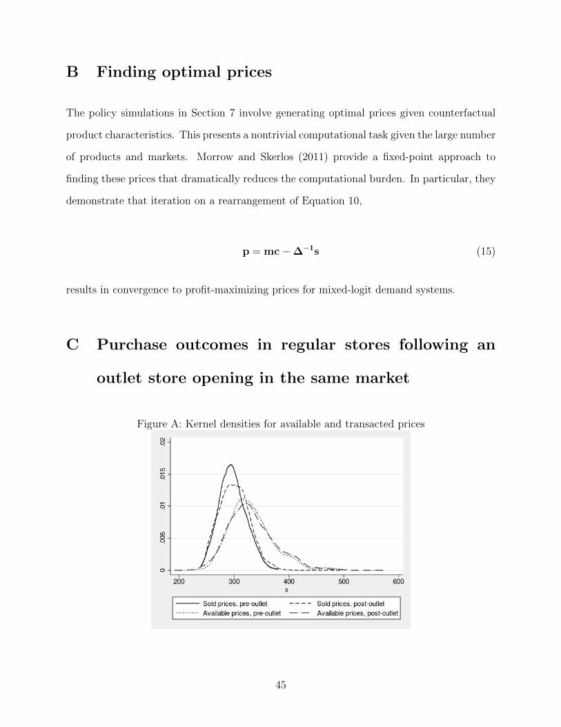
B Finding optimal prices

The policy simulations in Section 7 involve generating optimal prices given counterfactual

product characteristics. This presents a nontrivial computational task given the large number

of products and markets. Morrow and Skerlos (2011) provide a fixed-point approach to

finding these prices that dramatically reduces the computational burden. In particular, they

demonstrate that iteration on a rearrangement of Equation 10,

p = mc−∆−1s (15)

results in convergence to profit-maximizing prices for mixed-logit demand systems.

C Purchase outcomes in regular stores following an

outlet store opening in the same market

Figure A: Kernel densities for available and transacted prices

45

Figure A contains kernel densities of sold/transacted prices (denoting purchase outcomes)

and available prices (denoting product availability) in regular retail stores pre- and post-

the opening of an outlet store within the same market. There are a number of useful

observations to arise from inspecting this slice of the data. First, products bought in the

regular stores tend to be more expensive (despite relatively stable assortment) after an

outlet store opens—consistent with some cannibalization of the lower end by the outlet

store. Second, the magnitude of this shift is moderate—supporting the idea the outlet stores

primarily expand the market. Finally, the stability of available prices regardless of outlet

store presence is consistent with nationally determined assortment policies.

D Conversion at regular and outlet stores following

purchase at outlet store

Figure B: Histograms of days between conversion events

Figure B is a comparison of histograms of days between a purchase at an outlet store and (i)

a purchase at a regular store and (ii) another purchase at an outlet store, truncated at 100

days. I observe that the right hand side distribution is more skewed to the left, suggesting

that outlet stores do not disproportionately drive consumers to regular stores.

46

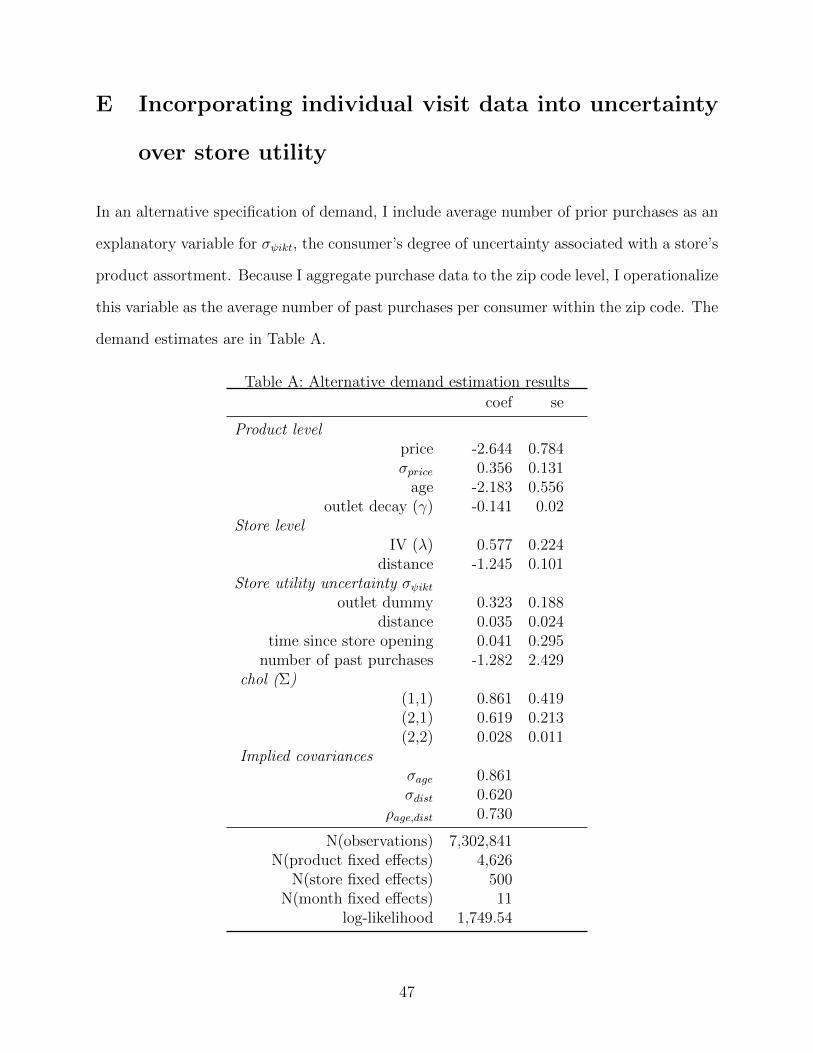
E Incorporating individual visit data into uncertainty

over store utility

In an alternative specification of demand, I include average number of prior purchases as an

explanatory variable for σψikt, the consumer’s degree of uncertainty associated with a store’s

product assortment. Because I aggregate purchase data to the zip code level, I operationalize

this variable as the average number of past purchases per consumer within the zip code. The

demand estimates are in Table A.

Table A: Alternative demand estimation results

coef se

Product levelprice -2.644 0.784σprice 0.356 0.131

age -2.183 0.556outlet decay (γ) -0.141 0.02

Store levelIV (λ) 0.577 0.224

distance -1.245 0.101Store utility uncertainty σψikt

outlet dummy 0.323 0.188distance 0.035 0.024

time since store opening 0.041 0.295number of past purchases -1.282 2.429

chol (Σ)(1,1) 0.861 0.419(2,1) 0.619 0.213(2,2) 0.028 0.011

Implied covariancesσage 0.861σdist 0.620

ρage,dist 0.730

N(observations) 7,302,841N(product fixed effects) 4,626

N(store fixed effects) 500N(month fixed effects) 11

log-likelihood 1,749.54

47