Why do Firms Hire using Referrals? Evidence from Bangladeshi

Garment Factories

Rachel Heath∗

January 18, 2013

Abstract

I argue that firms use referrals from current workers to mitigate a moral hazard problem.I develop a model in which referrals relax a limited liability constraint by allowing the firmto punish the referral provider if the recipient has low output. I test the model’s predictionsusing household survey data that I collected in Bangladesh. I can control for correlated wageshocks within a network and correlated unobserved type between the recipient and provider. Ireject the testable implications of models in which referrals help firms select unobservably goodworkers or are solely a non-wage benefit to providers.

JEL CODES: O12, J33, D22, D82

∗Department of Economics, University of Washington; rmheath@uw.edu. I am indebted to Mushfiq Mobarak,Mark Rosenzweig and Chris Udry for their guidance and suggestions. I also thank Treb Allen, Joe Altonji, PriyankaAnand, David Atkin, Gharad Bryan, Jishnu Das, Rahul Deb, Maya Eden, James Fenske, Tim Guinnane, Lisa Kahn,Dean Karlan, Fahad Khalil, Mark Klee, Fabian Lange, Jacques Lawarree, Richard Mansfield, Tyler McCormick,Melanie Morten, Nancy Qian, Gil Shapira, Vis Taraz, Melissa Tartari and various seminar participants for helpfulfeedback. The employees of Mitra and Associates in Dhaka provided invaluable help with data collection. Allremaining errors are my own.

1

1 Introduction

Firms in both developed and developing countries frequently use referrals from current workers to

fill job vacancies. However, little is known about why firms find this practice to be profitable. Since

hiring friends and family members of current workers can reinforce inequality (Calvo-Armengol and

Jackson, 2004), policy measures have been proposed to promote job opportunities to those who

lack quality social networks. For instance, policymakers who believe referrals reduce search costs

might require companies to publicize job openings. Such measures will succeed only if they address

the underlying reason firms hire using referrals.

I argue that firms use referrals to mitigate a moral hazard problem. I develop a model in which

the ability of a worker to leave for an alternate firm limits the original firm’s ability to punish a

worker after a bad outcome. Instead, a firm must provide incentives for high effort by raising wages

after a good outcome. This incentive scheme compels firms to lower initial wages in order to avoid

paying workers prohibitively high wages over the course of her employment, but a minimum wage

constraint limits firms’ ability to do this for lower-skilled workers.

I model a referral in which the provider of the referral agrees to forgo her own wage increase if the

referral recipient performs poorly. This agreement allows the firm to satisfy the recipient’s incentive-

compatibility constraint without violating the minimum wage constraint or paying prohibitively

high expected wage. If a social network can enforce contracts between its members, the recipient

will have to repay the provider later for any wage penalties she suffers. The recipient then acts as

though the punishment is levied on her own wages and thus exerts high effort in response. While

a sufficiently long relationship between the firm and worker would allow the firm to use multiple

periods of future wages to provide incentives for high effort and thus limit the need for the firms

to use referrals, employment spells are relatively short in many developing country labor markets.

For instance, in this paper’s empirical setting – the Bangladeshi garment industry – demand shocks

lead to frequent churning of workers between firms, workers often drop in and out of the labor force,

and careers are relatively short.

The contract between the firm, provider, and recipient in my model is analogous to group

liability in microfinance. In both cases, a formal institution takes advantage of social ties between

participants to gain leverage over a group of them. Varian (1990) shows that in a principal-agent

2

set-up, principals can use agents’ ability to monitor each other to reduce moral hazard. Bryan

et al. (2010) provide evidence of this social pressure in microfinance,1 which supports one of the

primary assumptions of my model: the recipient works hard if the provider has monetary gain from

her doing so. More broadly, this paper illustrates that firms can benefit from social ties between

workers.

The model generates several predictions on the labor market outcomes of referral providers

and recipients, which I test using household survey data that I collected from garment workers in

Bangladesh. I construct a retrospective panel for each worker that traces her monthly wage in each

factory, position, and referral relationship. The wage histories of the referral provider and recipient

can be matched if they live in the same bari (extended family residential compound).

I use these matched provider-recipient pairs to confirm the key testable premise of the model:

the provider is punished when the recipient performs poorly, so that the referral pair has positively

correlated wages. I compare the wages of bari members conditional on factory and individual

fixed effects to account for permanent unobserved heterogeneity at the factory and individual level.

I then conduct a different in difference test that assesses whether the correlation in these wage

residuals between a provider and recipient, relative to the correlation in wage residuals of other

bari members, is stronger when they are part of the referral relationship (versus when they are

working in different factories). This test allows me to account for within-bari wage shocks at a

certain time and the possibility that these shocks might be stronger if the bari members are in the

same factory or have ever been in a referral relationship. Detailed data on the type of work done

by each respondent further allow me to control for factory or industry-level wage shocks to workers

in a certain position or using a specific type of machine or within-factory shocks to a production

team.

This joint contract between the firm and referral pair has further testable implications for the

wage variance and observable skills of the provider and recipient. A provider’s wage is tied both to

her own output and that of the recipient. Therefore the wage variance of a provider will exceed that

of other workers of the same observable skill. Furthermore, since the wages of observably higher

skilled workers are higher relative to a constant minimum wage, firms can levy higher punishments

1Specifically, they offer a reward to a referral provider if the referral recipient repays back a loan, which increasesloan repayment rates. In one of the treatment arms they do not tell the participants about the reward until after thereferral has been made, so they can tell that the effect is due to social pressure and not selection.

3

on higher skilled workers without violating their own incentive compatibility constraint for high

effort. Referral providers are thus observably higher skilled than non-providers. Recipients, by

contrast, are observably lower skilled than other hired workers, since referrals allow the firm to hire

workers it would not otherwise.

While other hypothesized explanations for referrals – namely selection models (Montgomery

1991; Galenianos 2010) or patronage models (Goldberg, 1982) – can also predict the wage correlation

between a referral provider and recipient, I show that a moral hazard model has different predictions

on the wage path of referral recipients with tenure. Specifically, the moral hazard model in this

paper predicts that both the wage level and variance of referred workers increase with tenure

(relative to the wage level and variance of non-referred workers) as the firm uses both the recipient’s

own wages and those of the provider to provide incentives for high effort. By contrast, I develop

a selection model that predicts that as firms learn about non-referred workers after hiring, these

workers have either increasing wage variance or higher rates of dismissals than referred workers.

Neither of these patterns are not found in the data.2 A patronage model suggests that firms

use referrals to decrease the provider’s wage in order to pay recipients de-facto wages below the

minimum wage. However, this model provides no reason for firms to give wage increases to referral

recipients and thus cannot explain the increased wage level with tenure of the moral hazard model.

The empirical evidence that the provider’s wage reflects the recipient’s output confirms that

the provider has incentive to prevent the recipient from shirking. Previous literature arguing that

referrals provide information about recipients either proposes that the workers are passive and the

firm infers information about the recipient based on the provider’s type (Montgomery, 1991) or

must assume that the provider and firm’s incentives are aligned without having the data to validate

the assumption.3 This assumption may not always hold: referral providers may favor less qualified

family members (Beaman and Magruder, 2010) or refer workers who leave once a referral bonus is

received (Fafchamps and Moradi, 2009).

2By contrast, Simon and Warner (1992), Dustmann et al. (2009), and Pinkston et al. (2006) provide evidence ofdifferential learning about referral recipients. They study developed country labor markets, where the prevalence ofheterogeneous higher-skilled jobs likely make match quality and unobserved ability more important. They also lackthe matched provider-recipient pairs that provide evidence of moral hazard; therefore it is also possible that referralsaddress moral hazard in their scenario as well.

3For instance, Kugler (2003) assumes that referral recipients have a lower cost of effort due to peer pressurefrom providers. Simon and Warner (1992) and Dustmann et al (2009) posit that the provider truthfully reports therecipient’s type, which lowers the variance in the firm’s prior over the recipient’s ability.

4

This paper suggests a context where strong network ties are important in labor markets. While

in some contexts weak ties may be more able to provide non-redundant information about job

vacancies than close ties (Granovetter, 1973), the existence of networks in my model allows one

member to be punished for the actions of another. This mechanism depends on strong ties to

enforce implicit contracts through mutual acquaintances and frequent interactions. Accordingly,

almost half of the referrals in my data are from relatives living together in the same extended

family compound. My results then suggest that strong ties are important for job acquisition in

markets where jobs are relatively homogeneous but effort is difficult to induce through standard

mechanisms. Indeed, studies in the U. S. have found that job seekers of lower socioeconomic status

are more likely to use referrals from close relatives (Granovetter, 1983).

The rest of the paper proceeds as follows. In section 2, I provide information about labor

in the garment industry that is relevant to the model and empirical results. Section 3 develops

a theoretical model of moral hazard and shows how referrals can increase firm’s profits in that

environment. Section 4 contrasts the predictions of a moral hazard model with those of alternative

explanations for referrals: namely, patronage, selection, or search and matching models. Section

5 describes the data and section 6 explains the empirical strategy. I provide results in section 7.

Section 8 concludes.

2 Labor in the Garment Industry in Bangladesh

The labor force of the Bangladeshi garment industry has experienced explosive yearly growth of

17 percent since 1980. It has become an integral part of Bangladesh’s economy, constituting 13

percent of GDP and 75 percent of export earnings (Bangladesh Export Processing Bureau, 2009).

Garment production is labor-intensive. While specialized capital such as dyeing machines is used to

produce the cloth that will be sewn into garments, the garments themselves are typically assembled

and sewn by individuals at basic sewing machines. Production usually takes place in teams, which

typically consist of helpers (entry-level workers who cut lose threads or fetch supplies), operators

(who do the actual sewing), a quality control checker, and a supervisor.

A worker’s effort determines the quantity and quality of her output. It is relatively easy for firms

to assess the quantity of a worker’s output, but the quality of a garment can only be determined if

5

a quality checker examines it by hand. It is thus prohibitively costly for firms to observe workers’

effort perfectly, creating the potential for moral hazard. Firms’ ability to assess effort is further

complicated by the arrival of new orders with uncertain difficulty come in and instances where

a worker’s output is affected by others on her team. However, factory managers can use reports

from quality checkers and supervisors to assess worker’s effort and give rewards to the workers

who appear to have performed well. The theoretical model therefore considers allows firms to give

contracts based on output (which is correlated, but not perfectly, with a worker’s effort).

The key way that firms reward high output is through wage increases. Workers are typically paid

a monthly wage4 – 88 percent of workers in the sample receive one – and receive raises if they have

performed well. Sometimes raises are explicitly promised (conditional on good performance), and

other workers describe seeing colleagues in the same firm getting raises and anticipating that they

can do the same. Wages thus reflect – albeit noisily – the worker’s performance. This performance

assessment and subsequent wage updating happens relatively rapidly, as depicted in figure 1. By 12

months after hiring, for instance, only 36 percent of the workers who have remained with the firm

are still making the original wage offered to them upon hiring. Wages are relatively downwardly

nominally rigid; in only 0.67 percent of worker-months did the worker receive lower wages in the

next month, while 6.62 percent of worker-months culminated with a wage increase.5

The official minimum wage in Bangladesh at the time of the survey (August to October, 2009)

was 1662.5 taka per month, around 22 U.S. dollars. The minimum wage does appear to be binding:

only 9 out of 974 of the workers in the sample reported earning below the minimum wage, and figure

2 shows evidence of bunching in the wage distribution around the minimum wage. Anecdotally, even

if the government does not have the resources to enforce the minimum wage, upstream companies

fear the bad publicity that will result if journalists or activists discover that firms are paying below

the minimum wage.

There is rarely a formal application process for jobs in the garment industry. After hearing

4Explicit piece rates are therefore rare; only 10 percent of workers in my sample are paid per unit of production.Since firms would have to monitor workers under a piece-rate regime anyway to monitor the quality of their work,managers told me that piece rates are not worth the administrative cost, especially since they would have to redefinea new piece with each order.

5While this downward rigidity is not modeled explicitly, if wage decreases reduce workers’ effort (Bewley, 2002) orare otherwise undesirable to firms, then firms have even greater reason to provide incentives for effort by increasingwages after a good outcome rather than decreasing wages after a bad outcome. This further raises the cost to firmsof providing incentives for effort and increases the potential efficiency gain of referrals.

6

about a vacancy, hopeful workers show up at the factory and are typically given a short interview

and sometimes a “manual test” where they demonstrate their current sewing ability. Referrals are

common: 32 percent of workers received a referral in their current job. Sixty-five percent of referrals

came from relatives, most of which (and 45 percent of referrals overall) occurred between workers

living in the same extended family compound, called a bari. These workers often work in close

contact with each other; sixty percent of referral recipients began work on the same production

team as the provider of a referral. Receiving a referral is more common in entry level positions: 43

percent of helpers (vs. approximately 30 percent of operators and supervisors) received referrals.

By contrast, 44 percent of supervisors, 25 percent of operators, and only 10 percent of helpers have

provided referrals.

While I am unaware of the existence of contracts that explicitly tie the wage of the referral

provider to the performance of the referral recipient, workers do describe implicit contracts between

the firm, provider, and recipient that reflect the contracts modeled in this paper. Workers explain

that if a relative or friend has referred them into a job, they want to do perform well because the

referral provider looks bad if they do not. The provider may then be passed up for promotions or

raises which I model as wage penalty.6 When current workers were asked if they knew anyone who

they wouldn’t give a referral because she “wouldn’t be a good worker”, only 7 percent of respondents

said yes, while 85 percent said no, providing prima facie evidence that the performance of referred

workers relates to the effort of a recipient rather than a mechanism for selecting unobservably good

workers.

A final important characteristic of the labor market in Bangladeshi garment factories is the

relatively high turnover and short time that most workers spend in the labor force, which together

imply that the average time that a worker spends in particular factory is relatively low. The

median worker in my data has 38 months of total experience in the garment industry and 18

months experience in the same firm. A worker’s experience is often interrupted as workers spend

time out of the labor force in between employment spells, usually to deal with care-taking of

children, sick or the elderly. Thirty-one percent of current workers spent time out of the labor force

before their current job. Even garment workers who work continuously tend to switch factories

6This penalty does not necessarily contradict the nominal downward wage rigidity discussed earlier in this section.The provider receives a lower wages than she would have otherwise, which could have included a raise due to her ownperformance.

7

frequently, as competing factories get large orders and expand their labor force rapidly by poaching

workers from other factories. As shown in figure 1, by twelve months after the time of hiring, for

instance, only 64 percent of all hired workers who are still working in the garment industry remain

in that factory. Accordingly, the theoretical model in section 3 has two periods, giving firms the

option to use one period of future wages to induce effort, but not a long enough horizon to permit

for firms to be able to use multi-period contracts that induce the efficient level of effort even in the

presence of a lower bound on wages. That is, I consider the duration of employment spells to be

a middle ground between a spot market and a market in which a firm uses contracts spanning a

worker’s entire career to provide incentives for effort (Lazear, 1979).

3 Model

The model has two periods, and firms use higher wages in the second period to provide incentives

for high effort in the first. However, since workers have the option to leave and work for another

firm in the second period, limiting firms’ ability to punish workers after a bad outcome, firms must

provide incentives for high effort by increasing wages after a good outcome. This means that second

period wages that satisfy the incentive-compatibility constraint for effort are relatively high, and

firms must decrease the first period wages to avoid paying workers more in expectation than their

output. This wage scheme generates the relatively high average returns to experience found in the

industry (5.8 percent per year) and fits with workers’ reports that firms reward good workers with

raises.

However, the minimum wage limits firms’ ability to use this wage scheme for observably lower

skilled workers who have lower output and thus are paid lower wages. The firm will not be able to

provide incentives for high effort for these workers without paying them more than their output,

absent a referral. This referral allows the firm to punish the provider if the recipient has low output,

thus satisfying the recipient’s incentive compatibility constraint for high effort with lower expected

second period wages than would be required without a referral and allowing the firm to hire workers

it would not otherwise.

8

3.1 Set-up

In each of the two periods, output is given by y = θ +X, where θ is a worker’s observable quality

and X is a binary random variable, X ∈ {xh, xl}, with xh > xl. In each period, workers can

choose between two effort levels, eh or el. If the worker chooses eh, the probability of xh is αh. If

a worker chooses el, the probability of xh is αl, with αh > αl. For notational convenience, I define

the worker’s expected output at high effort to be πh and the worker’s expected output at low effort

to be πl. That is,

πh = αhxh + (1− αh)xl

πl = αlxh + (1− αl)xl

Each workers works for two periods. Between the first and the second period of work, a worker

can choose whether to stay with the current firm or leave and work with another firm. Firms

must offer a worker a wage before the period’s work take place, but can make second period wages

contingent on first period output. Specifically, the firm can offer a menu where the worker receives

w1 in the first period and in the second period earns

w2 =

w2h if X1 = xh

w2l if X1 = xl

Labor markets are competitive, so wage competition between firms bids wages up to a worker’s

expected production. I also assume that firms can commit to the wage contract, so that the worker

is not worried that the firm will renege on a given w2 wage offer.7 There is also a lower bound of

w on wages.8

Low effort has zero cost to workers, while high effort costs c. Workers are risk neutral9 and

utility is separable in expected earnings and effort cost. The worker discounts wages in the second

7The fact that fellow workers notice good work and whether it is rewarded helps make firms’ offers credible. Iffirms did not follow through on this implicit agreement, workers would notice and the firm’s reputation would suffer,leading workers to choose to work in other firms.

8One possible interpretation of this constraint is w = 0: workers are credit-constrained and they cannot be chargedto work. However, gains from referrals will be even greater if there exists a w which is strictly greater than zero, suchas a minimum wage.

9This assumption is made for analytical tractability. Adding risk aversion would only compound the moral hazardproblem and reinforce the importance of referrals in providing incentives for high effort.

9

period at rate δ ≤ 1, yielding utility of high and low effort respectively:

u(eh) = w1 − c+ δ(αhw2h + (1− αh)w2l)

u(el) = w1 + δ(αlw2h + (1− αl)w2l)

3.2 Non-Referred Workers

After output is realized from the first period, a worker can choose to stay at the initial firm or work

for another firm for one more period of work. The original firm can provide a worker incentives

to work hard in the first period by offering a w2h that is sufficiently high, relative to w2l, to make

high effort incentive-compatible:

−c+ δ(αhw2h + (1− αh)w2l

)≥ δ

(αlw2h + (1− αl)w2l

)(1)

w2h ≥ w2l +c

δ(αh − αl)

Akin to a back-loaded compensation model, a worker works hard in the first period for the promise

of higher future wages. Note that even though the worker is paid less than her output in the first

period, firms’ ability to commit to high wages means that the worker decides where to work based

on total wages and not just first period wages.

In the second period, an outside firm would bid wages up to the worker’s second period output

with low effort of w0(θ) = θ + πl,10 as long as this amount is above the minimum wage w.11 Thus

any wage below this amount offered to the worker in the second period by her original firm will

be rejected in favor of an alternative firm, and so the minimum earnings a worker can get after a

bad outcome is w0(θ).12 Accordingly, the firm must offer a w2h of at least w0(θ) plus the wedge

10I assume parameter values such that any worker worthwhile to hire and induce effort in during the first periodis worthwhile to hire for one period with low effort. See equation 5.

11The utility of workers with θ + πl < w, who wouldn’t be hired by another firm in the second period, is given bythe value of their outside option. I develop the role of outside options more in appendix B, focusing in particular ondetermining the parameter values that rule out a solution in which some workers with θ+πl < w are hired with higheffort, because their outside option is so much worse than the wage they would be making in garment work. Whilethe testable implications of the model would still go through in this case – there will still be some workers the firmcannot punish severely enough – the visual interpretation of the model given in figures 3 through 5 is clearer if therelationship between θ and high effort is monotonic.

12The moral hazard problem requires some limit on a firm’s ability to punish workers after a bad outcome. I modelthis as the possibility that a worker can leave for another firm. This seems reasonable, given that it is unlikely thatworkers could commit to stay with a firm (even if firms can commit to future wages). However, even if workers couldcommit to stay with firms, the minimum wage would still serve as a lower bound on wages in the second period and

10

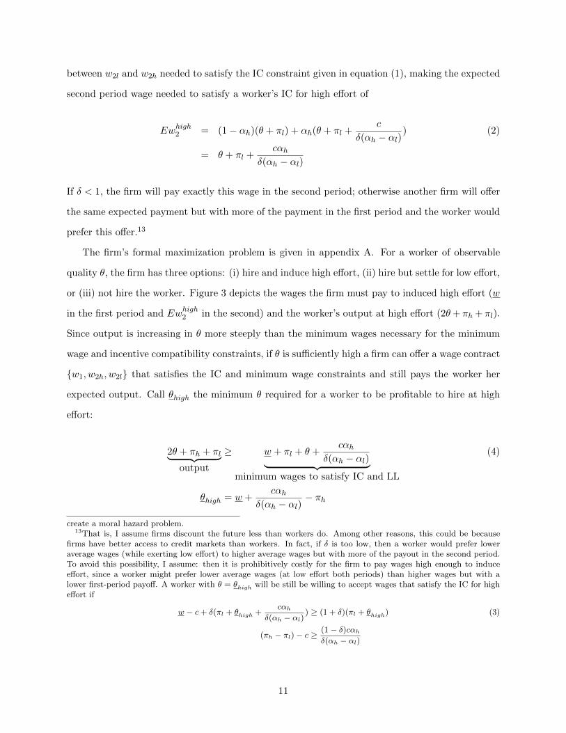
between w2l and w2h needed to satisfy the IC constraint given in equation (1), making the expected

second period wage needed to satisfy a worker’s IC for high effort of

Ewhigh2 = (1− αh)(θ + πl) + αh(θ + πl +c

δ(αh − αl)) (2)

= θ + πl +cαh

δ(αh − αl)

If δ < 1, the firm will pay exactly this wage in the second period; otherwise another firm will offer

the same expected payment but with more of the payment in the first period and the worker would

prefer this offer.13

The firm’s formal maximization problem is given in appendix A. For a worker of observable

quality θ, the firm has three options: (i) hire and induce high effort, (ii) hire but settle for low effort,

or (iii) not hire the worker. Figure 3 depicts the wages the firm must pay to induced high effort (w

in the first period and Ewhigh2 in the second) and the worker’s output at high effort (2θ+ πh + πl).

Since output is increasing in θ more steeply than the minimum wages necessary for the minimum

wage and incentive compatibility constraints, if θ is sufficiently high a firm can offer a wage contract

{w1, w2h, w2l} that satisfies the IC and minimum wage constraints and still pays the worker her

expected output. Call θhigh the minimum θ required for a worker to be profitable to hire at high

effort:

2θ + πh + πl︸ ︷︷ ︸output

≥ w + πl + θ +cαh

δ(αh − αl)︸ ︷︷ ︸minimum wages to satisfy IC and LL

(4)

θhigh = w +cαh

δ(αh − αl)− πh

create a moral hazard problem.13That is, I assume firms discount the future less than workers do. Among other reasons, this could be because

firms have better access to credit markets than workers. In fact, if δ is too low, then a worker would prefer loweraverage wages (while exerting low effort) to higher average wages but with more of the payout in the second period.To avoid this possibility, I assume: then it is prohibitively costly for the firm to pay wages high enough to induceeffort, since a worker might prefer lower average wages (at low effort both periods) than higher wages but with alower first-period payoff. A worker with θ = θhigh will be still be willing to accept wages that satisfy the IC for higheffort if

w − c+ δ(πl + θhigh +cαh

δ(αh − αl)) ≥ (1 + δ)(πl + θhigh) (3)

(πh − πl) − c ≥ (1 − δ)cαh

δ(αh − αl)

11

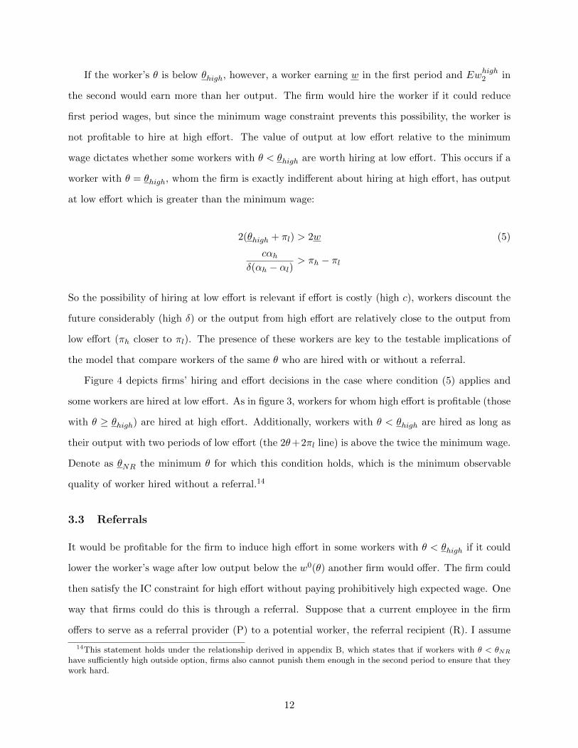
If the worker’s θ is below θhigh, however, a worker earning w in the first period and Ewhigh2 in

the second would earn more than her output. The firm would hire the worker if it could reduce

first period wages, but since the minimum wage constraint prevents this possibility, the worker is

not profitable to hire at high effort. The value of output at low effort relative to the minimum

wage dictates whether some workers with θ < θhigh are worth hiring at low effort. This occurs if a

worker with θ = θhigh, whom the firm is exactly indifferent about hiring at high effort, has output

at low effort which is greater than the minimum wage:

2(θhigh + πl) > 2w (5)

cαhδ(αh − αl)

> πh − πl

So the possibility of hiring at low effort is relevant if effort is costly (high c), workers discount the

future considerably (high δ) or the output from high effort are relatively close to the output from

low effort (πh closer to πl). The presence of these workers are key to the testable implications of

the model that compare workers of the same θ who are hired with or without a referral.

Figure 4 depicts firms’ hiring and effort decisions in the case where condition (5) applies and

some workers are hired at low effort. As in figure 3, workers for whom high effort is profitable (those

with θ ≥ θhigh) are hired at high effort. Additionally, workers with θ < θhigh are hired as long as

their output with two periods of low effort (the 2θ+2πl line) is above the twice the minimum wage.

Denote as θNR the minimum θ for which this condition holds, which is the minimum observable

quality of worker hired without a referral.14

3.3 Referrals

It would be profitable for the firm to induce high effort in some workers with θ < θhigh if it could

lower the worker’s wage after low output below the w0(θ) another firm would offer. The firm could

then satisfy the IC constraint for high effort without paying prohibitively high expected wage. One

way that firms could do this is through a referral. Suppose that a current employee in the firm

offers to serve as a referral provider (P) to a potential worker, the referral recipient (R). I assume

14This statement holds under the relationship derived in appendix B, which states that if workers with θ < θNR

have sufficiently high outside option, firms also cannot punish them enough in the second period to ensure that theywork hard.

12

that both P and R are part of a network whose members are playing a repeated game that allows

them to enforce contracts with each other that maximize the groups’ overall pay-off (Foster and

Rosenzweig, 2001). Then a provider is willing to allow her own wages to be decreased by some

punishment p if the recipient has low output, since the recipient will eventually have to repay her.15

Analogously to the firm’s problem with one worker, when considering a potential referral pair

with workers of observable quality (θP , θR) the firm can choose whether to hire and induce effort

in one or both workers. Appendix C details the full maximization problem. I will focus here on

the characterizing the scenario in which the firm finds it profitable to hire both the provider and

recipient and induce high effort in both. In this case the provider receives second period wages:

wP2 =

wP2h if P and R both have high output

wP2h − p if P has high, R has low

wP2l if P has low, R has high

wP2l − p if both P and R have low output

The recipient receives wR2h in the second period after high output and wR2l after low. The firm

can punish the provider to satisfy the recipient’s IC constraint for high effort, as long the provider’s

wage net of p does not drop below w0(θP ), which would prompt both workers to leave for another

firm. The firm can then satisfy the recipient’s IC constraint without the need to raise the recipient’s

expected second period wage (the EwR2 line on the graph) as high as it would need to be absent a

referral (the Ewhigh2 line on the graph).

The firm will then be able to induce high effort profitably in a recipient with θR < θhigh if θP

is high enough so that the workers’ joint output exceeds the wages the firm must pay in order to

satisfy IC constraints for both the recipient and provider without dropping either the recipient’s

wage or the provider’s wage net of p below w0(θR) and w0(θP ) respectively. That is if,

2(θP + θR + πl + πh) ≥ wR1 + wP1 + αhwP2h + (1− αh)wP2l + αhw

R2h + (1− αh)(wR2l − p) (6)

subject to the incentive compatibility constraints that high effort is worthwhile for the provider and

15Moreover, the referral creates a surplus – a worker is hired who wouldn’t be otherwise – so that the provider canbe made strictly better off once the reimbursement is made. While I will not model the side payments between theprovider and recipient that divide the surplus, the key point is that the referral can be beneficial for them both.

13

for the recipient (given both the recipient’s own wages and potential punishment of the provider),

that each worker’s outside option in the second period determines the maximum punishment, the

individual rationality constraint that the referral must give both workers higher utility than they

would get with the referral. The exact constraints are given in appendix C.

If (6) holds while satisfying these constraints, then the firm induces high effort in both workers.

Figure 5 depicts the minimum observable quality of recipient θR(θP ) that is profitable for the firm

to hire and provide incentives for high effort, given a provider of observable quality θP . This is the

recipient whose own IC would just bind after the firm levies the maximum punishment p on the

provider’s wage. This maximum punishment equals the difference between the amount the firm

must pay the provider to satisfy her own IC and the minimum wage (w+Ewhigh2 ) and her output.

It can then raise wP2l by p which guarantees that the provider will not leave in the second period

when she is facing punishment, even if she is already receiving wP2l after receiving low output herself.

The minimum observable quality of recipient θR(θP ) that is then profitable to induce effort has

output equal to the total wages of w in the first period and expected wage of EwR2 in the second.

Decreasing the provider’s wage is one particular way that the firm can punish the provider after

observing low output from the recipient. The firm could instead, for instance, fire the provider or

assign her to unpleasant tasks within the firm. However, if there is any firm-specific human capital

(or firing or replacement costs), then the firm has incentive to choose a punishment that retains

the worker (as wP2l − p ≥ w0(θ) ensures) but still makes the pair worse off than if the recipient had

high output. Accordingly, my main empirical focus is on punishment through wages. Providing

evidence that punishment takes place in this manner does not, of course, imply that punishment

does not occur in other ways. Instead, I provide evidence of one, potentially important, means

through which the firm punishes the provider.

3.4 Testable Implications

The joint contract offered to the provider and recipient generates several testable implications about

the observable quality and the wages of providers and recipients. The first set of implications provide

evidence that the provider’s wage reflects the recipient’s output:

1. Because the provider’s wage decreases by p when the recipient has low output, and thus

14

receives wR2l rather than wR2h, the wages (conditional on observed quality) of the provider and

recipient at a given time are positively correlated.

2. V ar(wP |θ) > V ar(w|θ). A provider’s wage reflects not just her own output, but the recipient’s

as well. For proof, see appendix D.2.

3. E(θ|hired and made referral) > E(θ|hired). A firm’s scope to punish a provider is increas-

ing in θ, so the higher θP , the lower is the minimum θR(θP ) from that worker and the more

willing is the firm to accept a referral from that worker. This result is also discussed in

appendix D.1.

A second set of testable implications show that firms provide referred workers wage schedules that

satisfy an IC constraint for high effort. This increased effort allows a firm to hire workers with

referrals that it wouldn’t otherwise be able to hire.

4. E(θ|hired with referral) < E(θ|hired). Because the firm can get positive profits from some

observably worse recipients than θNR, recipients on average have lower θ than other hired

workers. For proof, see appendix D.1.

5. The wage level of referral recipients is increasing with tenure, relative to non-recipients. The

firm provides incentives for effort both by increasing the recipient’s wage after a good outcome

and punishing the provider after a bad outcome. By contrast, the firm has no incentive to

provide wages to non referred workers, who are exerting low effort. For proof, see appendix

D.3.

6. The wage variance of referral recipients also increases with tenure. In addition to the increase

in average wages of referred workers, the wedge between wR2h and wR2l that appears in the

second period increases their wage variance, relative to the wages of non-referred workers

whose second period wage does not depend on output. For proof, also see appendix D.3.

The predictions on the wages of referral recipients are crucial in distinguishing a moral hazard

model from other reasons that firms might use referrals, in particular, from a selection model

and a patronage/nepotism model. That is, while selection and patronage models also predict

the provider’s wage reflects the recipient’s output and that referrals allow observably lower skilled

15

recipients be hired that would not be otherwise, they do not predict that the wage level and variance

of referral recipients increases with tenure relative to non-referred workers. The next section briefly

summarizes the predictions of a selection and a patronage models in a similar two-period set-up to

the moral hazard case, and explains why their predictions differ from a moral hazard model.

4 Contrasting the predictions of the Moral Hazard Model with

Alternative Models of Referrals

4.1 Selection

Much of the previous literature on referrals assumes that the referral provides information about

the recipient’s unobserved type. In some of these papers, the mechanism is correlated unobservable

types within a network (Montgomery 1991; Munshi 2003); the firm can estimate the recipient’s type

based on what it has learned about the type of the provider. However, while this model predicts

that there may be correlation between the wages of a referral pair even when they are not working

in the same factory, it cannot explain why this wage correlation is differentially stronger when they

are in the same factory together. Alternatively, the provider could be reporting the the recipient is

high type (Saloner, 1985). Firms would then know more about recipients before hiring16 and learn

more about non-recipients after hiring.

Appendix E characterizes this selection model. If there is any noise in the mapping between

type and output (i.e., sometimes high types have low output and sometimes low types have high

output), then providers must be punished when the recipient has low output in order to ensure

that only the good types are referred. This punishment predicts the same positive wage correlation

between referral recipient and provider as the moral hazard model, but the firm’s adjustment of

recipients’ wages yields different predictions on the wages and turnover of recipients after hiring.

Specifically, once the firm learns the true type of each worker, if the costs are low to replace a

worker, then the firm would fire the non-referred workers that it learns are low type, and there

would be higher turnover among non-referred workers. Alternatively, if replacement costs are high

16That is, firms cannot learn at least some of the information provided by the referral in any other way. Whilefirms do use manual tests (see section 2) to learn the dexterity and skills of potential hires, the referral would begiving information about motivation, attention to detail, and diligence, which cannot be measured in these tests.

16

enough that the firm chooses to retain the workers it learns are bad types, it still updates their

wages to reflect this new information. Then the wage variance of non-referred workers would spread

with tenure.

4.2 Patronage

Another possible model suggests that referrals allow firms to set de facto wages below the minimum

wage by lowering the provider’s wage by the difference between the minimum wage and its desired

wage for the recipient.17 The firm and the referral pair are both better off in this scenario, since

absent a referral the minimum wage would prevent firms from hiring all the workers it would like.

The positive correlation between the wages of the recipient and provider would then represent the

fact that the “fee” for the referral (as reflected in the lowering of the provider’s wages) is decreasing

in the quality of the recipient. However, those workers hired with a referral would always receive

the minimum wage, since the firm would actually prefer to pay them less than the minimum. So

there is no reason that the wages of referral recipients would increase with tenure relative to non-

recipients, as predicted by a moral hazard model. Moreover, if there is any reason wages of the

more valuable non-referred workers would increase with tenure,18 the wages of referred workers

would fall with tenure, relative to non-referred workers.

4.3 Search and Matching

While a full search and matching model is beyond the scope of this paper, I utilize the predictions

of the model of Dustmann et al. (2009). In their model, referred workers are not on average better

type than non-referred workers, but the firm has a more precise signal about the true productivity

of referred workers. Because referred workers are better matched with their jobs initially than

nonreferred workers, their wages are initially higher than those of non-referred workers, who are

willing to accept lower wages for the expectation of higher future wage growth (since they are

17Note that the moral hazard model presented in this paper also implies that referrals serve to offset the minimumwage: the referral provider might agree to a referral that decreases her current wage, since the recipient will agreeto repay her in the future. The question, then, is whether the empirical results could be explained by a patronagemodel of referrals in an environment where effort is perfectly observable.

18For instance, good workers could build up firm specific human capital more rapidly than bad workers. This seemsplausible, since entry level work is similar across all firms, whereas supervisors need to understand the details of thework done by a specific firm.

17

insured against low realizations of their productivity by the ability to leave the firm). So non-

referred workers are predicted to have higher wage growth than referred workers.

Note that while the Dustmann et al. (2009) and other search models don’t explicitly incorporate

joint contracts between the firm, provider, and recipient that would predict the positive wage

correlation of the other models considered, other components of a search model might lead to this

wage correlation. For instance, if the provider and recipient both have a specialized skill and the

factory uses the referral to fill that specialized skill at a time it has a particularly large demand

for it. In section 6.1 I argue that the detailed data I collected on the machine type, position,

and production team of the provider and recipient alleviate the concern that within-factory wage

shocks to certain types of workers generate the positive wage correlation in provider and recipient.

However if there was a wage shock to some component of worker type which is unobserved to the

econometrician and referrals are used to help find this type of worker, it is useful to note that this

type of search model has different implications for evolution of the wages of that referred worker

after hiring.

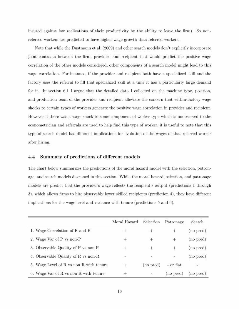
4.4 Summary of predictions of different models

The chart below summarizes the predictions of the moral hazard model with the selection, patron-

age, and search models discussed in this section. While the moral hazard, selection, and patronage

models are predict that the provider’s wage reflects the recipient’s output (predictions 1 through

3), which allows firms to hire observably lower skilled recipients (prediction 4), they have different

implications for the wage level and variance with tenure (predictions 5 and 6).

Moral Hazard Selection Patronage Search

1. Wage Correlation of R and P + + + (no pred)

2. Wage Var of P vs non-P + + + (no pred)

3. Observable Quality of P vs non-P + + + (no pred)

4. Observable Quality of R vs non-R - - - (no pred)

5. Wage Level of R vs non R with tenure + (no pred) - or flat -

6. Wage Var of R vs non R with tenure + - (no pred) (no pred)

18

5 Data and Summary Statistics

The data for this paper come from a household survey that I conducted, along with Mushfiq

Mobarak, of 1395 households in 60 villages in four subdistricts outside of Dhaka, Bangladesh.19

The survey took place from August to October, 2009. Households with current garment workers

were oversampled, yielding 972 garment workers in total in the sample. Each sampled garment

worker was asked about her entire employment and wage history. Specifically, she was asked to

list the dates she worked in each factory and spell-specific information about each such as how

she got the job (including detailed information about the referral) and the nature of work done.20

A factory-specific code was recorded, allowing me to match the outcomes of workers in the same

factory for the empirical tests that require comparisons of outcomes of workers working in the

same factory. The sampled workers worked in 892 factories all together during their careers. Of

these factories, 198 had more than one sampled worker at a particular time period and 95 had a

within-bari referral with both members captured in the data.

A worker is also asked if she ever changed wages within the factory, and if so, in what month each

wage change occurred and whether there was also a change in position associated with the wage

change. The surveys I observed suggested that workers did not much have difficulty remembering

past wages. Wage information is very salient to workers, most of whom are working outside the

home or for a regular salary for the first time and whose wages represent substantial improvements

to household well-being. However, there is still likely some measurement error, and I discuss the

impact it may have on my results in section 6.

Together, these data yield a retrospective panel of a worker’s monthly wage and other outcomes

in each of her factories, positions, and referral relationships since she began working. This work

history is crucial for several aspects of my identification strategy. Primarily, multiple observations

per worker allow me to include worker fixed effects and observing a pair of workers both in and out

of a referral relationship allows me to control for correlated unobservables when testing whether

their wage correlation is higher in the factory with the referral relationship. Additionally, I know

19Specifically, Savar and Dhamrai subdistricts in Dhaka District and Gazipur Sadar and Kaliakur in GazipurDistrict. For use in other projects, 44 of the villages were within commuting distance of garment factories, and 16were not. Details of the sampling procedure and survey are given in Heath (2011).

20If a worker worked in a given factory for two spells, with a spell at another factory in between (which did occur42 times), the questions were asked separately about each spell. So if a worker has referred in one spell but not theother, or by different people in each spell, this was recorded.

19

the timing of worker’s decisions to leave the labor force temporarily, allowing me to use these

decisions as a proxy for the worker’s decision to leave the labor force permanently. Analyzing the

relationship between referrals and the decision to leave the labor force temporarily provides some

evidence on the influence of attrition out of the labor force in the retrospective panel. I also know

how much time workers spent out of the labor force between jobs, so that I can also control for

actual experience when constructing measures of a worker’s observable skill in the empirical tests.

This is important in an industry where the returns to experience are high but workers often spend

time out of the labor force between employment spells.

The sampling unit for the survey was the bari. A bari is an extended family compound,

where each component household lives separately but households share cooking facilities and other

communal spaces. The median number of bari members in sampled baris was 18, with a first

quartile of 9 people and the third quartile of 33. Any time a worker indicated receiving a referral

from a bari member who was also surveyed, the identity of the provider was recorded. Therefore,

in employment spells where the surveyed worker received a referral from someone living in the bari

and working in the garment industry at the time of the survey, the work history of the recipient

can be matched to the work history of the provider.

The word used for “referral” in the survey was the Bangla word suparish, which most literally

translates as “recommendation.” However, given that I do not know of any factories with policies

of making a recommendation/referral official, I did not try to determine whether the factory knew

about the bond between workers. That is, I instructed the enumerators to err on the side of coding

as a referral any time the recipient found out about the job through a current worker in the factory.

The survey form allowed the respondent to name at maximum one referral provider per employment

spell.21

Table 1 provides information on the personal and job characteristics of workers who have re-

ceived referrals, those who have given referrals, and those who neither gave nor received referrals.

One pattern that emerges from the table is that workers do not seem to use referrals to gain infor-

mation about unfamiliar labor markets. In fact, those who were born in the city in which they are

21In section 7.1 I argue that if I have coded as a “referral” some instances where the firm does not know aboutthe bond between the provider and recipient or if the firm does actually make referral contracts between multipleproviders and recipients, it would only work against me finding the relationship that I do between the provider andrecipient’s wages.

20

currently residing are more likely to have received a referral than those who have migrated to their

current city. Workers are also no more likely to use referrals in jobs that are further from their

current residence, as measured in commuting time.

6 Empirical Strategy

6.1 Testing for Punishment of Provider

The test for punishment of the provider based on performance of the recipient (prediction 1) is

whether the recipient’s wage (conditional on observable characteristics) predicts the provider’s

wage (also conditional on observable characteristics) at a given point in time. I examine whether

this holds among the 45 percent of referrals in the sample that are between bari members, which

is the sample where I can match provider and recipient. Specifically, I first obtain obtain wage

residuals conditional on observable variables (the θ in my model), since the model’s prediction

on the wage correlation of R and P is conditional on each worker’s θ. I include both factory and

individual fixed effects in this specification to allow for the possibility that some factories pay higher

average wages than others (and may use referrals differentially more or less) and for unobserved

individual-level characteristics (which may be correlated between the provider and recipient).

log(wift) = β0 + δf + γi + β1experienceift + β2experience2ift + εift (7)

Denote the residual from this regression as w̃ift. I then run a regression where the unit of observation

is the wage residual w̃ of any pair of bari members i and j that are both working in the garment

industry at the same time t. Specifically, I regress the w̃ift of one of the pair on the w̃jft of the

other, and allow the effect of w̃jft to vary based on whether i and j are in the same factory,

whether there has ever been a referral between i and j, and whether i and j are currently in a

referral relationship22.

w̃ift =γ1 w̃jft + γ2 w̃jft × ever referralij (8)

+ γ3 w̃jft × same factoryijt + γ4 w̃jft × referralijt + uift

22Recall that a referral in my model is by definition between two workers in the same factory.

21

The following table shows the number of observations which identify the different interaction

terms in the regression. While the majority of the observations in this regression are bari members

in different factories between whom there was never a referral, whose role in the regression is only

to identify industry-wide wage shocks, there is still a large absolute number of referral pairs, both

together and outside of the same factory.

ever referred = 0 ever referred = 1

same factory = 0 56,299 366

same factory = 1 8,199 380

Since individual and factory-level heterogeneity have already been accounted for in equation

(7), equation (8) tells us whether the wage of one bari members is above her average (relative

to others in the same factory) when another bari member’s wage is above her average (relative

to others in the same factory). This could happen, for instance, if bari members have correlated

productivity shocks (due to, for example, a contagious illness). If so, then γ1 would be positive.

The wjft×ever referralij term allows this correlation to be stronger between members of a referral

pair, even when that referral relationship is not in place. The wjft × same factoryijt term lets

the correlation in within-bari shocks be stronger between bari members who are working in the

same factory. If after accounting for each of these shocks, there is still a differentially stronger

wage correlation among members of a referral relationship, then γ4 > 0 and I conclude that there

is punishment of the provider based on the performance of the recipient. This test is valid if

w̃jft×referralijt is uncorrelated with the error term uift, conditional on the wjft×same factoryijt

and wjft × ever referralij terms. That is, the referral itself must be the only reason that two

members of a referral pair can have differentially stronger correlation in wages during the referral

relationship.

One might be concerned that this condition fails due to wage shocks to observable job charac-

teristics within the factory – namely, to production team, position, or machine type. That is, the

referral pair may do similar work and a within-factory or industry-wide wage shock to that type

of work leads to differentially stronger wage correlation between the bari pair relative to other bari

members working in the same factory. For instance, the provider might have trained the recipient

to sew using a specialized type of machine and their factory gets a large order that necessitates

heavy use of that machine, prompting both the provider and recipient’s wages to increase at the

22

same time. To address this concern, I allow for within-factory and industry-wide wage shocks to

machine or position by including interactions of w̃jft and w̃jft × same factoryijt with indicators

for same machineijt and same positionijt and verify that the referral pair still has differentially

stronger wage correlation during the referral relationship.

It is not possible to do the exact same test for the production team, since I know whether two

bari members were on the same production team only if there was a referral between the two.

However, I can interact an indicator for same teamijt with w̃jft × referralijt in equation 8 to

test whether the wages of a referral pair who are not on the same production team are still more

strongly correlated than the wages of other bari members working together in the same factory

(who may or may not be on the same team). If so, it is unlikely that production complementarities

are driving the correlation in wages between the provider and recipient, since their wages remain

more strongly correlated than other bari members even when they are not working together on the

same team.

This test requires retrospective wage data in order to compare the wages of a provider and

recipient in the same factory to their wages when they are not in the same factory. While using

retrospective wage data from current garment workers raises the possibility of attrition bias – if one

member of a referral pair drops out of the garment industry then I cannot include their wages here

– a very particular pattern of turnover would be required to bias the w̃jft × referralijt coefficient

away from zero. That is, to make the wages of the provider and recipient appear more strongly

correlated than they would without attrition, either the provider or recipient would have to drop

out of the labor market when they received a wage shock in the opposite direction of the other.

For instance, the recipient would have to drop out of the labor market when her wages would have

been low, but only when the provider has high wages. Using data on workers’ decisions to drop

out of the labor force temporarily as a proxy for the decision to leave the labor force permanently,

there is no evidence of any of these patterns.23

While the variable referralijt reported by the participants may not perfectly capture the notion

of a referral modeled theoretically, such misclassification is unlikely to bias the w̃jft × referralijt23That is, in a probit regression where the dependent variable is equal to one if the worker leaves the labor force

temporarily in a particular month (conditional on working in the previous month), the wage residual of the recipienthas no effect on whether a provider leaves the labor force temporarily, and similarly the wage residual of a providerhas no effect on whether a recipient leaves the labor force temporarily.

23

coefficient away from zero. For instance, in some cases the respondent might have reported having

been referred, but the provider only passed along information about the job without notifying the

firm of her connection to the recipient. The firm would then not be able to punish the provider

based on performance of the recipient. However considering these instances as referrals would bias

the coefficient on w̃jft×referralijt toward zero. Similarly, if in actuality the firm punishes multiple

providers if the recipient has low output but only one is considered to be a provider in regression

(8), then the wages of the control pairs also reflect wage effects of a referral, and the estimated

wage effects of a referral are smaller than they would be otherwise.

Retrospective wage information based on recall data also likely contains measurement error.

However, there would need to be differentially stronger correlation in the noise components of the

wage reports of a bari pair (relative to other bari members working in the same factory at the same

time) to yield a differentially stronger wage correlation between the referral pair. To mitigate this

possibility, surveys were done with each worker independently to mitigate the type of information

sharing that might occur differentially between a referral pair and lead to correlated measurement

error. The remaining recall error likely represents classical measurement error and would only bias

the coefficient on w̃jft × referralijt toward zero.

6.2 Wage Variance

Predictions 2 and 5 pertain to the wage variance of referral providers and recipients, conditional

on their observed skills. So I first condition out observable measures of skill by estimating a wage

equation for worker i in factory f :

log(wif ) = β0 + δf + β1experienceif + β2experience2if + β3maleif + β4educationif + εif (9)

Since this test does not require past wages that allow multiple observations per worker–unlike in

the test for punishment of the provider–I use only current wages in estimating (9) to avoid concerns

about selective attrition. For instance, providers may be less likely to drop out of the labor market

after a bad wage shock since they don’t want to leave the friends they have referred alone in the

factory. I then test whether the squared residual ε̂2if (an estimate for wage variance) increases if

the worker made a referral.

24

ε̂2if = α1x′if β̂ + α2 made referralif + α3 referredif + uif (10)

I do this test conditional on the worker’s fitted wage x′iftβ̂, since many theories of the labor market

would predict that wage variance is higher among high-skilled groups (Juhn et al., 1993). The model

predicts that both recipients and providers have higher wage variance than other hired workers of

the same θ, which would yield α2 > 0 and α3 > 0.

Since the prediction on the wage variance of recipients is more nuanced – their wage variance

grows with tenure, relative to the wage variance of non-referred workers – I further test additionally

whether within-worker wage variance increases for non-referred workers. This test shows that the

higher wage variance for recipients is not due to permanent characteristics that are reported to the

firm by the provider (or observed to the firm but not the econometrician), which would result in

larger wage variance for recipients that begins on hiring.

Specifically, I assess whether the squared difference between a worker’s wage residual after a

certain time in the firm (t1 = 3, 6, and 12 months) and the worker’s initial wage offer at time t0

varies between recipients and non-referred workers.

(w̃it1 − w̃it0)2 = β0 + β1referredi + εi (11)

These relatively short time windows yields estimates that are relatively uncorrupted by the selection

of which workers remain in the firm that long but is long enough to reflect firms’ initial observation

of worker’s output and their subsequent wage updating. The model predicts β1 > 0: the wage

variance of referred workers raises with tenure, relative to that of non-referred workers.24

6.3 Observable Quality

To test predictions 3 and 4, which relate to the observable quality (θ in my model) of providers

and recipients, I consider separately two measures of skill: experience and education25. So for each

24I also control for education, experience, and sex to guarantee that any differences in wage variance with tenureof workers with these characteristics are not driving the coefficient on referred.

25While literacy and numeracy are not strictly required (except for supervisors, who need to keep written records),employers say that educated workers are more likely be proficient “floaters.” Floaters are individuals who fill in invarious parts of the production chain when other workers are absent or after a special order has come in. An educatedworker can more easily learn the work from a pattern rather from than watching it be done.

25

worker-employment spell, I estimate:

educif = β0 + δf + β1referredif + β2made referralif + β3maleif + εif (12)

experienceif = β0 + δf + β1referredif + β2made referralif + β3maleif + εif (13)

where experience is measured at the beginning of employment. I include factory fixed effects to

compare providers and recipients to other workers in the same factory. The model predicts β1 < 0

and β2 > 0 in both regressions: providers should have more education and experience than other

hired workers, while recipients should have less.

6.4 Wage Level with Tenure

Prediction 6 is that the wage level of referral recipients increases with tenure. I again look at

wages a short window after hiring (3, 6, and 12 months) to assuage fears that differential attrition

is driving changes in wage levels of stayers versus non-stayers. To further allay concerns that

differential attrition is driving these results, I repeat each specification only including workers who

have survived in the firm up until that point so that the identification of the differential trend of

referred workers with tenure only comes from comparison of workers who remain in the firm.

logwift =β0 + δf + γ1referredift + γ2tenureift + γ3referredift × tenureift (14)

+ β1experienceift + β2experience2ift + β3maleift + β4educationift

The model predicts γ3 > 0: the wages of referred workers raise with tenure, relative to those of

non-referred workers.

7 Results

7.1 Punishment of Provider

Table 2 reports results from equation (8), a regression of one bari member’s residual wage w̃it on

the residual wage w̃jt of another bari member working in the garment industry at the same time,

and on interactions of w̃jt with whether i and j were in the same factory, whether there has ever

26

been a referral between i and j, and an interaction between the indicator for same factory and

whether there has been a referral between i and j. Standard errors are calculated by bootstrapping

the two-stage procedure. Specifically, I take repeated samples with replacement from the set of

monthly wage observations. For each replicate I first estimate the wages conditional on observables

to get the w̃ift’s, construct pairs of wage observations for baris with multiple members chosen in

that replicate, and then estimate equation (8). This procedure, analogous to a block bootstrap,

preserves the dependent nature of the wage pairs data by ensuring that if a wage observation is

selected, all pairs of wage observations involving that worker at that time will also be in the sample.

In column 1, we see that the coefficients on w̃jft and w̃jft × ever referralijt are close to zero

and insignificant: there is no evidence of correlated wage shocks among bari members in different

factories, whether or not there was once a referral between the two workers. The coefficients among

bari members in the same factory (both with and without a referral), by contrast, are positive. To

help interpret these coefficients, consider three bari members in the same factory: P referred R,

whereas C works in the same factory but did not participate in a referral with either P or R. So

a 10 percent increase in R’s wage (above her mean wage, compared to other workers in the same

factory) corresponds to an increase of 0.566 percentage points in C’s wage (above her mean wage,

compared to other workers in the same factory). This effect is much stronger between the provider

and recipient, yielding a positive coefficient on the variable of interest, w̃jft× referralijt. So if R’s

wage goes up by 10 percent, P’s wage goes up 3.295 percentage points more than it does after a 10

percent increase in C’s wage.

Column (2) adds interactions between w̃jft and w̃jft×same factoryijt and an indicator variable

for whether the pair is using the same machine to allow for industry-wide and within-factory wage

shocks to workers skilled in using a particular machine. After including these effects the interaction

between w̃jft and same factoryijt becomes zero, so the wage correlation between bari members in

the same factory is indeed driven by within-factory wage shocks to workers using the same machine

type. However, there is no evidence that wage shocks to certain machine types are driving the

referral effect; the coefficient on w̃jft × referralijt remains unchanged. Column (3) suggests that

there are industry-wide, but not within factory, wage shocks to workers in a specific position; the

coefficient on w̃jt×same positionijt is positive. The referral effect w̃jft×referralijt again remains

unchanged, suggesting that a tendency of referred worked to work in the same position is not

27

driving their wage correlation. Finally, column (4) verifies that the w̃jft × referralijt coefficient is

still significant even among pairs not working on the same production team.

One further robustness check addresses a potential concern that firms hire workers with referrals

at particular times in the production cycle, such as after receiving a big order, which would heighten

the wage correlation between all workers at that factory at that time. This pattern of wage shocks

suggests a specification that compares referred workers to other workers in the same factory at

the same time. Accordingly, in table 3 I reestimate equation (8) using the wage observations in

bari-factories pairs at times in which there was at least one referral between bari members in the

factory. The coefficient on w̃jft×referralijt then identifies the wage correlation of the referral pair

compared to the wage correlation of other bari members in the same factory as the referral pair

at the same time. While I lose the ability to use the w̃jft × ever referralij coefficient to allow for

differentially stronger wage between a referral pair, this test provides evidence that the results in

table 2 are not driven by wage shocks occuring to the the entire factory at times when it is using

referrals. Reassuringly, the coefficient on w̃jft × referralijt is very similar in this sample.

The first column shows that when one member of a referral pair’s wage increases by 10 percent,

the other’s wage increases by 2.541 percent more than it would after an equivalent wage increase

from another bari member in the same factory. Analagously to table 2, columns two and three

include interactions of w̃jt with an indicator for whether the two are using the same machine or

work in the same position to demonstrate that the wage effects of the referral are not driven by

differentially stronger shocks to machine or position in factories using referrals. Column 4 again

shows that the differentially stronger correlation in wage between the referral pair relative to other

workers in the same factory is not only present in referral pairs on the same production team.

7.2 Unexplained Wage Variance

Table 4 gives the results from regression (10), which tests whether the unexplained wage variance–

the residual ε̂2if from a first stage wage regression–varies with fitted wage x′if β̂ and whether the

worker has made or received a referral. Column (1) indicates that those giving and receiving

referrals have higher wage variance than others with their same predicted wage. The coefficient

of 0.021 on referred and the coefficient of 0.022 on made referral are both large, relative to the

average squared wage residual of 0.068. Column (2) includes interactions between made referral

28

and position dummies, addressing the potential concern that the variance result for providers is

driven primarily by supervisors. If so, we might be concerned that the more capable supervisors are

both allowed to give referrals and also manage larger teams or receive wages that are more closely

tied to their team’s performance, leading to higher wage variance absent effects from the referral.

However, there is no evidence that the effect of giving a referral on wage variance is larger among

supervisors.

Table 5 reports the estimated coefficients from equation 11, which further tests whether the

overall higher wage variance reported in table 4 represents increasing wage variance with tenure

(versus higher wage variance that appears from initial wage offer). Wage variance does increase

with tenure. The estimated effects of a referral on the squared wage change from initial to 3, 6,

and 12 month wages are highly significant and very large, greater than the mean squared change

for the 3 and 6 month cases and seventy percent of the mean change after 12 months.

7.3 Observable Quality

Table 6 reports results from regressions (12) and (13), which test for differences in education

and experience between providers and recipients versus other hired workers in the same factory.

Columns (1) and (4) show that referral recipients on average have 0.67 fewer years of education and

0.59 fewer years of experience than other workers in the same factory. By contrast, providers have

on average 0.30 more years of education and 0.51 more years of experience than other workers in

the same factory. In columns (2) and (5), I include position dummies. While a literal interpretation

of the model would say that only a worker’s observable quality θ matters in determining her ability

to give, or need for, a referral (and not her θ relative to others in the same position) the inclusion

of position dummies shows that observable differences in recipients and providers are not only

determined by variation in θ across positions.26 While smaller in magnitude, the results are still

negative and significant for recipients and positive (although insignificant) for providers. Columns

(3) and (6) show that providers are observably better and recipients are observably worse than

other garment workers in the same bari. These results confirm that bari members with mid-range

26That is, a worker’s observable quality is increasing in her position level, and section 2 points out that givingreferrals is more common in higher positions and less common in lower positions. If the results on observable qualitydid not hold within position, then they would also be consistent with a story in which referrals are a way to makeentry level workers feel comfortable, by ensuring that they have an experienced provider around.

29

values of θ constitute the control group for the referral pairs in equation (8); they are good enough

not to need a referral, but not observably good enough to be able to give one.

7.4 Wage Levels with Tenure

Table 7 reports the results of equation 14 which compares changes in the wage level of referral

recipients with those of non-referred workers after 3, 6, and 12 months. Whether the sample

includes the wages from all workers or only wages for those workers who have remained in the firm

for that long, the tenure × referred coefficient is large and positive. It is significant in each case

using each window for the regressions including only stayers, and after 12 months for both samples.

The estimated coefficient on the tenure× referred after 12 months, for example, shows that after

a year in a firm, the wage of a referred worker have gone up 4.56 percentage points (12 months

times a coefficient of 0.0038 per month) more than that of an observably identical worker who did

not receive a referral but has remained in the firm for those 12 months. This increase corresponds

to the higher second period wages for referred workers who have had high output, relative to the

flat wage schedule offered to non-referred workers.

8 Conclusion

The results of this paper indicate that referrals can minimize a moral hazard problem caused by

firms’ inability to perfectly observe workers’ effort. Referrals provide allow the firms to use the

provider’s wages to provide the recipient incentives for high effort, a useful tool in an industry

where employment spells are relatively short. I provide empirical evidence from data I collected

from the garment industry in Bangladesh that the poor performance of a recipient lowers both her

own wage and that of the provider. The joint contract ensures the recipient will work hard even

though the firm’s ability to punish her is limited, and thus allows the firm to hire observably lower

skilled workers than it would otherwise hire.

While the empirical work was limited to the garment industry in Bangladesh, there is little

reason to believe that firms’ potential to use referrals to solve moral hazard is limited to this

context. Many labor markets, particularly in the developing world, are also characterized by the

high turnover that makes effort difficult to induce using long-term contracts. Anthropological

30

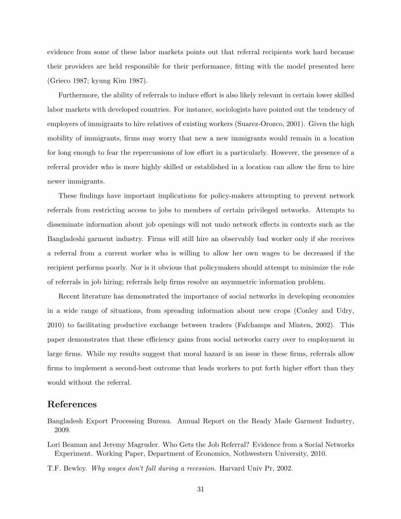
evidence from some of these labor markets points out that referral recipients work hard because

their providers are held responsible for their performance, fitting with the model presented here

(Grieco 1987; kyung Kim 1987).

Furthermore, the ability of referrals to induce effort is also likely relevant in certain lower skilled

labor markets with developed countries. For instance, sociologists have pointed out the tendency of

employers of immigrants to hire relatives of existing workers (Suarez-Orozco, 2001). Given the high

mobility of immigrants, firms may worry that new a new immigrants would remain in a location

for long enough to fear the repercussions of low effort in a particularly. However, the presence of a

referral provider who is more highly skilled or established in a location can allow the firm to hire

newer immigrants.

These findings have important implications for policy-makers attempting to prevent network

referrals from restricting access to jobs to members of certain privileged networks. Attempts to

disseminate information about job openings will not undo network effects in contexts such as the

Bangladeshi garment industry. Firms will still hire an observably bad worker only if she receives

a referral from a current worker who is willing to allow her own wages to be decreased if the

recipient performs poorly. Nor is it obvious that policymakers should attempt to minimize the role

of referrals in job hiring; referrals help firms resolve an asymmetric information problem.

Recent literature has demonstrated the importance of social networks in developing economies

in a wide range of situations, from spreading information about new crops (Conley and Udry,

2010) to facilitating productive exchange between traders (Fafchamps and Minten, 2002). This

paper demonstrates that these efficiency gains from social networks carry over to employment in

large firms. While my results suggest that moral hazard is an issue in these firms, referrals allow

firms to implement a second-best outcome that leads workers to put forth higher effort than they

would without the referral.

References

Bangladesh Export Processing Bureau. Annual Report on the Ready Made Garment Industry,2009.

Lori Beaman and Jeremy Magruder. Who Gets the Job Referral? Evidence from a Social NetworksExperiment. Working Paper, Department of Economics, Nothwestern University, 2010.

T.F. Bewley. Why wages don’t fall during a recession. Harvard Univ Pr, 2002.

31

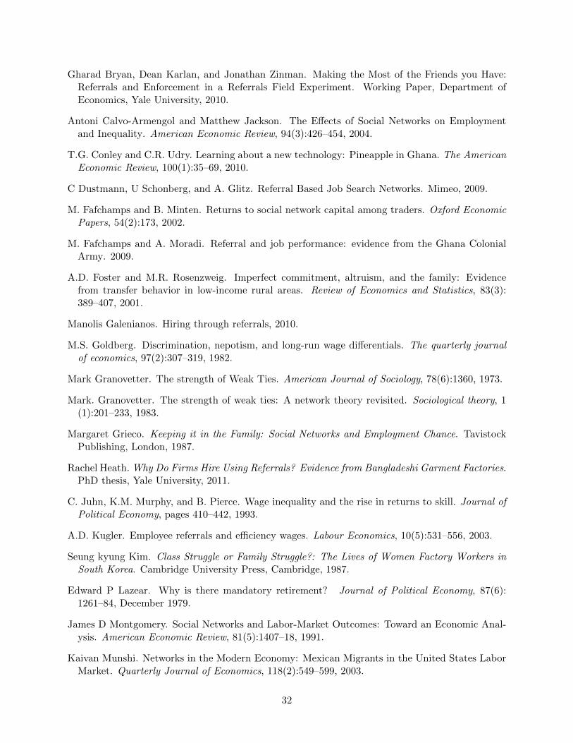
Gharad Bryan, Dean Karlan, and Jonathan Zinman. Making the Most of the Friends you Have:Referrals and Enforcement in a Referrals Field Experiment. Working Paper, Department ofEconomics, Yale University, 2010.

Antoni Calvo-Armengol and Matthew Jackson. The Effects of Social Networks on Employmentand Inequality. American Economic Review, 94(3):426–454, 2004.

T.G. Conley and C.R. Udry. Learning about a new technology: Pineapple in Ghana. The AmericanEconomic Review, 100(1):35–69, 2010.

C Dustmann, U Schonberg, and A. Glitz. Referral Based Job Search Networks. Mimeo, 2009.

M. Fafchamps and B. Minten. Returns to social network capital among traders. Oxford EconomicPapers, 54(2):173, 2002.

M. Fafchamps and A. Moradi. Referral and job performance: evidence from the Ghana ColonialArmy. 2009.

A.D. Foster and M.R. Rosenzweig. Imperfect commitment, altruism, and the family: Evidencefrom transfer behavior in low-income rural areas. Review of Economics and Statistics, 83(3):389–407, 2001.

Manolis Galenianos. Hiring through referrals, 2010.

M.S. Goldberg. Discrimination, nepotism, and long-run wage differentials. The quarterly journalof economics, 97(2):307–319, 1982.

Mark Granovetter. The strength of Weak Ties. American Journal of Sociology, 78(6):1360, 1973.

Mark. Granovetter. The strength of weak ties: A network theory revisited. Sociological theory, 1(1):201–233, 1983.

Margaret Grieco. Keeping it in the Family: Social Networks and Employment Chance. TavistockPublishing, London, 1987.

Rachel Heath. Why Do Firms Hire Using Referrals? Evidence from Bangladeshi Garment Factories.PhD thesis, Yale University, 2011.

C. Juhn, K.M. Murphy, and B. Pierce. Wage inequality and the rise in returns to skill. Journal ofPolitical Economy, pages 410–442, 1993.

A.D. Kugler. Employee referrals and efficiency wages. Labour Economics, 10(5):531–556, 2003.

Seung kyung Kim. Class Struggle or Family Struggle?: The Lives of Women Factory Workers inSouth Korea. Cambridge University Press, Cambridge, 1987.

Edward P Lazear. Why is there mandatory retirement? Journal of Political Economy, 87(6):1261–84, December 1979.

James D Montgomery. Social Networks and Labor-Market Outcomes: Toward an Economic Anal-ysis. American Economic Review, 81(5):1407–18, 1991.

Kaivan Munshi. Networks in the Modern Economy: Mexican Migrants in the United States LaborMarket. Quarterly Journal of Economics, 118(2):549–599, 2003.

32

J.C. Pinkston, United States. Bureau of Labor Statistics. Office of Employment, and UnemploymentStatistics. How Much Do Employers Learn from Referrals? 2006.

G. Saloner. Old boy networks as screening mechanisms. Journal of Labor Economics, 3(3):255–267,1985.

C.J. Simon and J.T. Warner. Matchmaker, matchmaker: The effect of old boy networks on jobmatch quality, earnings, and tenure. Journal of Labor Economics, 10(3):306–330, 1992.

M.M. Suarez-Orozco. Interdisciplinary perspectives on the new immigration. Routledge., 2001.

H. Varian. Monitoring agents with other agents. Journal of institutional and theoretical economics,146:153–174, 1990.

A Firm’s Problem, Baseline Case with No Referrals

For a worker of a given observable quality θ, the firm can choose between hiring the worker and

inducing high effort, hiring the worker but accepting low effort, or not hiring the worker:

π = max(

0,

max 2θ + πh + πl − w1 − αhw2h − (1− αh)w2l

subject to δ(αhw2h + (1− αh)w2l

)− c ≥ δ

(αlw2h + (1− αl)w2l

)(IC)

w2h, w2l ≥ max(w0(θ), w̃(θ)) (max punishment)

w1, w2h, w2l ≥ w (min wage)

2θ + πh + πl = w1 + αhw2h + (1− αh)w2l, (zero profit)

max 2θ + 2πl − w1 − αlw2h − (1− αl)w2l

subject to w1, w2h, w2l ≥ w (LL)

2θ + 2πl = w1 + αlw2h + (1− αl)w2l (zero profit))

B Outside options

Consider the role of the workers’ outside option w̃(θ), which they would earn if their original firm

fires them in the second period and are not worthwhile for another firm to hire (θ+πl < w). If the

firm wants to induce high effort in one of these workers, it must pay her a w2h = w̃(θ) + cδ(αh−αl)

.

33

This is not profitable if the worker’s output from high effort in the first and low in the second (with

αh probability) is less than the firm’s expected wage bill for that worker, w in the first period and

αhw2h in the second:

w + αh

(w̃(θ) +

c

δ(αh − αl)

)≥ θ + πh + αh(θ + πl) (15)

The graphical depictions of the model given in figures 3 through 5 assume this constraint holds, so

that only workers with θ > θhigh are profitable to hire with high effort. If this constraint does not

hold, so that some workers with θ+πl < w are profitable to hire at high effort, referrals still improve

efficiency: the firm would use the ability to punish a provider to drive down the recipient’s utility

after a bad outcome below w̃(θ) and thus be able to profitably hire some workers that it could not

otherwise. These testable implications of the model would remain the same, since referrals would

still allow the firm to induce high effort in workers with w− πl < θ < θhigh, who would be exerting

low effort absent the referral.

C Firm’s Problem with Referrals

The firm’s set of possible options are

(i) hire both R and P and induce effort in both

(ii) hire both and induce effort only in P

(iii) hire both and induce effort only in R

(iv) hire both but induce effort in neither

(v) hire only P with high effort

(vi) hire only P with low effort

(vii) hire only R with high effort

(viii) hire only R with low effort

The predictions of the model focus on scenario (i). This decision is profitable if

maxwR

1 ,wP1 ,w

P2h,w

P2l,w

R2h,w

R2l,p

2(θP +θR+πl+πh)−wR1 −wP1 −αhwP2h−(1−αh)wP2l−αhwR2h−(1−αh)(wR2l−p)

34

subject to:

wP2h ≥ wP2l +c

δ(αh − αl)(IC, P )

wR2h ≥ (wR2l − p) +c

δ(αh − αl)(IC,R)

wP2h, wP2h − p, wP2l, wP2l − p ≥ max(w0(θP ), w̃(θP )) (max punishment, P)

wR2h, wR2l ≥ max(w0(θR), w̃(θR)) (max punishment, R)

wP1 , wP2h, (w

P2h − p), wP2l, (wP2l − p) ≥ w (minimum wage, P )

wR1 , wR2h, w

R2l ≥ w (minimum wage,R)

wR1 + αhwR2h + (1− αh)(wR2l − p) + wP1 + αhw

P2h + (1− αh)wP2l (IR)

≥ max(w1(θP ) + αhw2h(θP ) + (1− αh)w2l, 2w̃(θP )

)+ max

(w1(θR) + αhw2h(θR) + (1− αh)w2l(θR), 2w̃(θR)

)

is greater than or equal to zero. The IR constraint says that in expectation, participating in the

referral must be profitable for the recipient and provider together. That is, their wages in the

referral must exceed their payoffs from not participating, which are equal to the max of the wages

they would be offered by other firms, or their outside options.

D Proofs

Proposition D.1. Workers with θR < θNR can be profitably hired by the firm if they have a referral

from a provider of sufficiently high θP .

Proof. Consider a worker with θR < θNR who would not be hired absent a referral. The firm can

profitably hire this worker if the constraints in case (i) are satisfied, and both workers exert high

effort. Suppose specifically that worker had a referral from a provider with observable quality θP

35

and the firm sets wages:

wR1 = w

wP1 = w

wR2l = w

wR2h = w − p+ cδ(αh−αl)

wP2l = w0(θP ) + p

wP2h = wP2l + cδ(αh−αl)

That is, the minimum wage constraints bind for R in the first period and the second period after

low output, and for P in the first period. Additionally, the IC constraints for high effort just bind

for P and R. For a given punishment p, the firm increases wP2l (relative to w0(θP )) by p in order

to insure that the provider doesn’t leave in the second period, even if she and the recipient both

had low output in the first period. Then with w0(θP ) = θP + πl, the observable quality of referral

provider for which joint output just equals the wage bill is:

2θR + 2θP + 2πh + 2πl = 2w︸︷︷︸first period wages

+ wP2l +cαh

δ(αh − αl)︸ ︷︷ ︸second period wages for provider

(16)

+ w − (wP2l − θP − πl) +cαh

δ(αh − αl)︸ ︷︷ ︸second period wages for recipient

θR(θP ) =3

2w +

cαhδ(αh − αl)

− πl2− πh −

θP2

Then since θR(θP ) is decreasing in θP , for any θR, a referral in which the output from both workers

exerting high effort is greater than the wages the firm would need to satisfy the IC and minimum

wage constraints is possible if θP is sufficiently high. The IR constraint for the θR(θP ) derived in

equation 16 holds as long as the pair’s period 1 utility from both working (with high effort) and

earning the wages given above is greater than their utility without the referral (where P would be

hired at high effort since θP > θhigh, and R would receive the value of her outside option since

36

θR < θNR):

2w − 2c+ δ(w + θP + πl + 2cαh

δ(αh − αl)) ≥ (17)

(1 + δ)w̃(θR) + θP + πh −cαh

δ(αh − αl)− c+ δ(θP + πl +

cαhδ(αh − αl)

)

(2 + δ)w − c+cαh(1 + δ)

δ(αh − αl)≥ θP + πh + (1 + δ)w̃(θR)

Whether this constraint is satisfied depends on the value of R’s outside option (w̃(θR)) relative to

the minimum wage and the discount rate (since P has to delay more of her compensation than she

would absent the referral). If this constraint fails, for the θR(θP ) derived in equation 16, then the

θR(θP ) that makes (17) hold with equality would be the lowest θR accepted from a provider with

θP . If δ = 1, this constraint simplifies to

2θR + πh + πl − c ≥ 2w̃(θR) (18)

Accordingly, if workers are relatively patient (δ close to 1) and θP is sufficiently high, then the

referral is profitable as long as R’s output in garments is above her outside option.

Note that there is a possibility for other types of referral contracts to be profitable. For instance,

the firm could hire R for only one period and charge P a punishment of cδ(αh−αl)

if R has low output.

However, since they key testable implication would be the same (workers with θR < θNR would be

hired), I will not further analyze these contracts.

Proposition D.2. V ar(wP |θ) > V ar(w|θ)

Proof. Without a referral, the second-period wage distribution of a worker of observable quality θP

will be:

w =

θP + πl + cδ(αh−αl)

with probability αh

θP + πl with probability 1− αh

yielding variance αh(1 − αh) cδ(αh−αl)

. If this worker gives a referral, then she will receive some

punishment p (whose level depends on the θR) if the recipient has low output. Her observed

37

second-period wage distribution will then be:

w =

wP2l + cδ(αh−αl)

with probability α2h

wP2l + cδ(αh−αl)

− p with probability αh(1− αh)

wP2l with probability αh(1− αh)

wP2l − p with probability (1− αh)2

which yields wage variance αh(1−αh)p cδ(αh−αl)

. For any positive p, this is larger than the variance

with no referral.

Proposition D.3. For workers with θNR < θ < θhigh, referrals increase both wage level and

variance with tenure: E(wR2 |θ) − E(wR1 |θ) > E(w2|θ) − E(w1|θ) and (E(wR2 |θ) − E(wR1 |θ))2 >

(E(w2|θ)− E(w1|θ))2

Proof. Consider a worker with observable quality θR, where θNR < θR < θhigh. Without a referral,

that worker will be hired with low effort and be paid her output πl + θR in each period. The

minimum p required for that worker to be hired – call this p(θR) – sets her output equal to the

wages net of this punishment.

2θR + πh + πl = θR + w − p+cαh

δ(αh − αl)(19)

p(θR) = w +cαh

δ(αh − αl)− πh − θR

Since θ > w − πl = θNR, and cαhδ(αh−αl)

≤ cδ(αh−αl)

, then p < cδ(αh−αl)

and therefore wRh > wRl .

That is, the firm satisfies R’s IC for high effort both by punishing the provider and creating a

wedge between wRh and wRl , which increases wage variance among referral recipients relative to the

second period wage a non-referred worker gets that does not depend on output. Note also that R’s

expected wage

EwR2 = (1− αh)w + αh(w +c

δ(αh − αl)) = w +

cαhδ(αh − αl)

is strictly greater than her first period wage of w. This reflects both the fact that the punishment

levied on P does not appear in R’s wage and also that the firm uses higher second period wages

after a good outcome as provide incentives for effort for R. So the wage trajectory for a recipient

is increasing with tenure, relative to the flat wage schedule the firm gives a worker with the same

38

θR who does not have a referral.

E Selection Model

Production remains the same as in the moral hazard framework except for the fact that effort is

now a function of observable quality θ and unobservable quality ε, where ε can be high or low.

A worker’s type is revealed (to the current firm and the market overall)27 between the first and

second periods. As in the moral hazard set-up competition between firms bids the worker’s wage

up to her expected productivity. Let 0 < β < 1 be the proportion of high types in the population.

Analogous to the moral hazard framework, the probability of high output if ε = εhigh is αh, which

is greater than the probability of high output if ε = εlow. Define πh = αhεh + (1 − αh)εl and

πl = αlεh + (1 − αl)εl. In the second period of work, the firm will retain all workers for whom

θ+ ε ≥ w. Workers with θ such that θ+ εl ≥ w are hired and retained in the second period whether

they are low type or not. Workers with θ + εl < w are not worth retaining in the second period if

they turn out to be low type but are worthwhile to hire in the first with some possibility they are

high type if

θ + Eπ − w + β(θ + πh)− w ≥ 0 (20)

θNR = w − Eπ − βπh1 + β

So workers with θNR ≤ θ ≤ w − εl are dismissed in the second period, whereas workers with

θNR ≥ w − εl are retained and then paid their newly revealed productivity.

Referrals allow the firms to hire workers with θ < θNR that it knows are high type. Then the

firm sets a punishment p on providers whose recipients had low output that makes it incentive-

compatible to refer high-type workers but not low type.28 Again assuming that R and P can

27If learning were asymmetric, the results would persist as long as there is any reason that firms would like toupdate wages to reflect this new information about her productivity. This would occur as long as outside firmslearned anything about workers producitivty. Even if learning is entirely limited to the the current firm, that firmmay still pay higher-productivity workers more if there is some chance workers will choose to leave after receiving awage offer.

28A low type worker has no incentive to receive a referral in this model, she would prefer for the firm to have noinformation and pay her according to the expected productivity of a random worker.

39

perfectly enforce contracts between each other, the IC and PC constraints for a referral are:

−(1− αh)p+ w + θ + πh ≥ 0 (PC: Do refer high types) (21)

−(1− αl)p+ w ≥ 0 (IC: Don’t refer low types) (22)

In the second period, once the market also knows the recipient’s type, the firm must pay the recipient

her output θ + πh.29 Accordingly, conditional on θ, there is no wage variance of referred workers

in the second period, yielding a lower variance increase with tenure than with the non-referred

workers.

29Note that, like the moral hazard model, the selection model also contains an element of the patronage model:the firm will hire workers whose output (even with high type) is below the minimum wage θ+ πh < w because it can“charge” the referrer an amount equal to the difference between the recipient’s output and the minimum wage. Still,since referrals are also a selection mechanism, referred workers are of higher type than nonreferred workers, and weshould see differential learning as firms learn the type of non-referred workers and update wages accordingly.

40

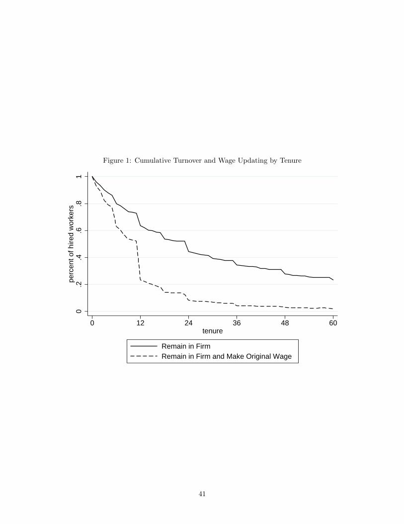
Figure 1: Cumulative Turnover and Wage Updating by Tenure

0.2

.4.6

.81

perc

ent o

f hire

d w

orke

rs

0 12 24 36 48 60tenure

Remain in FirmRemain in Firm and Make Original Wage

41

Figure 2: Wage Distribution for Referral Recipients and Non-Referred Workers

050

100

150

Fre

quen

cy

0 2000 4000 6000 8000 10000Wage in Taka

Referred

050

100

150

Fre

quen

cy

0 2000 4000 6000 8000 10000Wage in Taka

Non−Referred

42

w

θ

w

θhigh

Outputhigh = 2θ + πh + πl

Ew2high = θ+ πl +

w1

w

Figure 3: Observable quality and incentives for high effort

43

2w

w

θ θNR

Outputlow = 2θ + 2πl

Ew2high =θ+ πl +

Outputhigh 2θ + πh + πl

θhigh

w

Figure 4: Observable quality and hiring of non-referred workers

44

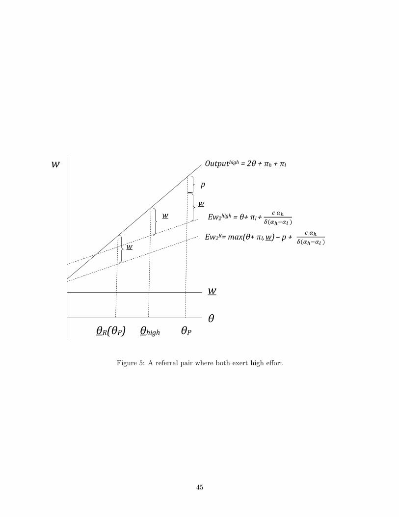
w

w

θ

w

θhigh

Outputhigh = 2θ + πh + πl

p

w

θP

Ew2high = θ+ πl +

𝑐 𝛼ℎ

𝛿(𝛼ℎ−𝛼𝑙 )

θR(θP)

)

Ew2R= max(θ+ πl, w) – p + 𝑐 𝛼ℎ

𝛿(𝛼ℎ−𝛼𝑙 )

w

Figure 5: A referral pair where both exert high effort

45

Table 1: Summary Statistics, Recipients, Providers and Other Workers

recipient providera neither overall

male 0.436 0.609 0.373 0.433[0.029] [0.032] [0.022] [0.016]

experience (months) 14.017 26.285 20.376 19.931[1.576] [2.377] [1.518] [1.072]

education (years) 5.354 6.617 5.799 5.870[0.203] [0.253] [0.155] [0.116]

married 0.736 0.865 0.769 0.776[0.025] [0.023] [0.019] [0.014]

has a child 0.340 0.457 0.415 0.397[0.027] [0.033] [0.023] [0.016]

age 26.017 28.448 25.369 26.029[0.482] [0.543] [0.363] [0.267]

originally from current village 0.112 0.100 0.059 0.078[0.018] [0.020] [0.011] [0.009]

either parent any education 0.520 0.567 0.493 0.515[0.029] [0.033] [0.023] [0.016]

good relations with managementb 0.840 0.853 0.808 0.829[0.021] [0.023] [0.018] [0.012]

appointment letterc 0.330 0.494 0.293 0.346[0.027] [0.033] [0.021] [0.015]

took manual testd 0.340 0.463 0.462 0.429[0.027] [0.033] [0.023] [0.016]

commute time (minutes) 18.170 19.316 18.868 18.887[0.719] [0.874] [0.566] [0.419]

typical daily hours of work 11.801 11.805 11.642 11.722[0.123] [0.149] [0.113] [0.077]

N 306 231 485 967percent 31.6 23.9 50.2 100

Notes: (a) Workers who both received and gave referrals appear in both of the first two columns.(b) worker reported “good” or “excellent” relationship, out of possible choices “very bad”, “bad”, “okay”, “good”,“excellent”(c) an appointment letter states that the worker cannot be dismissed without cause(d) a manual test taken before an employment spell consists of an employer sitting the worker down in front of asewing machine, pre-hiring, and asking her to demonstrate the specific skills and maneuvers that she knows

46

Table 2: Wage correlation between provider and recipient

Dep. Var is wage residual w̃ift(1) (2) (3) (4)

w̃jft 0.0006 0.0088 -0.0252*** 0.0006[0.005] [0.006] [0.006] [0.005]

w̃jft × ever referralij 0.0051 0.0106 -0.0206 0.0063[0.027] [0.028] [0.028] [0.033]

w̃jft × same factoryijt 0.0566*** 0.0060*** 0.0503*** 0.0566***[0.012] [0.015] [0.015] [0.012]

w̃jft × referralijt 0.3195*** 0.3110*** 0.3390*** 0.3200***[0.074] [0.077] [0.076] [0.078]

w̃jft × same machineijt -.0.0219***[0.009]

w̃jft × same factoryijt × same machineijt 0.1073***[0.028]

w̃jft × same positionijt 0.0685***[0.010]

w̃jft × same factoryijt × same positionijt 0.0194[0.031]

w̃jft × referralijt × same teamijt -0.0045[0.064]

Observations 66,784 66,784 66,784 66,784R-squared 0.001 0.001 0.002 0.001

Stars indicate significance: *** p<0.01, ** p<0.05, * p<0.1

The unit of observation is a matched pair of the wage residual w̃ift of a bari member and the wage residual w̃jft of

another bari member working in the garment industry in the same month. Residuals are from the first stage wage

regression given by equation 7.

Bootstrap standard errors in brackets, constructed by taking repeated samples of monthly wage observations and then

constructing the bari member pairs for each sample chosen (then repeating 100 times)

47

Table 3: Comparing workers currently in referral relationships to other workers in same factory

Dep. Var is wage residual w̃ift(1) (2) (3) (4)

w̃jft 0.0523 0.0440 0.0551** 0.0523[0.035] [0.042] [0.028] [0.035]

w̃jft × referralijt 0.2541*** 0.2545*** 0.2537*** 0.2880***[0.053] [0.053] [0.050] [0.069]

w̃jft × same machineijt 0.0205[0.049]

w̃jft × same positionijt -0.0073[0.041]

w̃jft × referralijt × same teamijt -0.0740[0.080]

Observations 1,520 1,520 1,520 1,520R-squared 0.032 0.032 0.032 0.033

Stars indicate significance: *** p<0.01, ** p<0.05, * p<0.1

The unit of observation is a matched pair of the wage residual w̃ift of a bari member who was in the same factory

and a referral between two members of that worker’s bari and the wage residual w̃jft of another bari member working

in the same factory in the same month. Residuals are from the first stage wage regression given by equation 7.

Bootstrap standard errors in brackets, constructed by taking repeated samples of monthly wage observations and then

constructing the bari member pairs for each sample chosen (then repeating 100 times)

48

Table 4: Unexplained variance, providers and recipients

Dependent Var: ε̂2if from first stage wage regression

(1) (2)

x′if β̂ 0.0490*** 0.0570***

[0.0162] [0.0188]referred 0.0214** 0.0199**

[0.0099] [0.0100]made referral 0.0220* 0.0332

[0.0114] [0.0327]operator -0.0163

[0.0126]supervisor -0.00613

[0.0236]operator × made referral -0.0101

[0.0352]supervisor × made referral -0.0200

[0.0434]

Mean Dep Var 0.069 0.069Observations 939 939R-squared 0.023 0.026

Stars indicate significance: *** p<0.01, ** p<0.05, * p<0.1. The dependent variable is a worker’s squared wage

residual from equation 9, which is then regressed on the worker’s fitted wage x′if β̂ from the same regression, along

with dummy variables for referred and made referral.

49

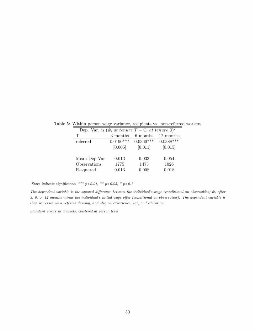
Table 5: Within person wage variance, recipients vs. non-referred workers

Dep. Var. is (w̃i at tenure T − w̃i at tenure 0)2

T 3 months 6 months 12 months

referred 0.0190*** 0.0360*** 0.0388***[0.005] [0.011] [0.015]

Mean Dep Var 0.013 0.033 0.054Observations 1775 1473 1026R-squared 0.013 0.008 0.018

Stars indicate significance: *** p<0.01, ** p<0.05, * p<0.1

The dependent variable is the squared difference between the individual’s wage (conditional on observables) w̃i after

3, 6, or 12 months minus the individual’s initial wage offer (conditional on observables). The dependent variable is

then regressed on a referred dummy, and also on experience, sex, and education.

Standard errors in brackets, clustered at person level

50

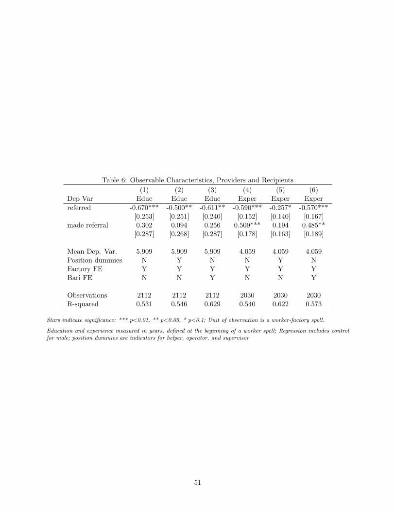
Table 6: Observable Characteristics, Providers and Recipients

(1) (2) (3) (4) (5) (6)Dep Var Educ Educ Educ Exper Exper Exper

referred -0.670*** -0.500** -0.611** -0.590*** -0.257* -0.570***[0.253] [0.251] [0.240] [0.152] [0.140] [0.167]

made referral 0.302 0.094 0.256 0.509*** 0.194 0.485**[0.287] [0.268] [0.287] [0.178] [0.163] [0.189]

Mean Dep. Var. 5.909 5.909 5.909 4.059 4.059 4.059Position dummies N Y N N Y NFactory FE Y Y Y Y Y YBari FE N N Y N N Y

Observations 2112 2112 2112 2030 2030 2030R-squared 0.531 0.546 0.629 0.540 0.622 0.573

Stars indicate significance: *** p<0.01, ** p<0.05, * p<0.1; Unit of observation is a worker-factory spell.

Education and experience measured in years, defined at the beginning of a worker spell; Regression includes controlfor male; position dummies are indicators for helper, operator, and supervisor

51

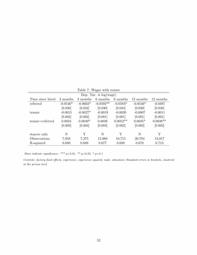
Table 7: Wages with tenure

Dep. Var. is log(wage)Time since hired 3 months 3 months 6 months 6 months 12 months 12 months

referred -0.0546* -0.0602* -0.0592** -0.0583* -0.0546* -0.0387[0.030] [0.032] [0.030] [0.034] [0.030] [0.040]

tenure -0.0015 -0.0027* -0.0019 -0.0020 -0.0007 -0.0011[0.002] [0.002] [0.001] [0.001] [0.001] [0.001]

tenure×referred 0.0024 0.0049* 0.0038 0.0052** 0.0035* 0.0038**[0.003] [0.003] [0.003] [0.002] [0.002] [0.002]

stayers only N Y N Y N YObservations 7,958 7,375 12,968 10,715 20,794 13,917R-squared 0.680 0.688 0.677 0.688 0.678 0.713

Stars indicate significance: *** p<0.01, ** p<0.05, * p<0.1

Controls: factory fixed effects, experience, experience squared, male, education; Standard errors in brackets, clustered

at the person level

52