
Whole genome analyses using PopGenome and VCF files
29
Whole genome analyses using PopGenome and VCF files Bastian Pfeifer July 3, 2017 1
Transcript of Whole genome analyses using PopGenome and VCF files

Whole genome analyses using PopGenomeand VCF files
Bastian Pfeifer
July 3, 2017
1

Contents1 PopGenome classes 4
2 Reading tabixed VCF files (readVCF) 42.1 filename . . . . . . . . . . . . . . . . . . . . . . . . . . . . . . . . . . . . . 52.2 numcols . . . . . . . . . . . . . . . . . . . . . . . . . . . . . . . . . . . . . 52.3 tid . . . . . . . . . . . . . . . . . . . . . . . . . . . . . . . . . . . . . . . . 52.4 frompos . . . . . . . . . . . . . . . . . . . . . . . . . . . . . . . . . . . . . 52.5 topos . . . . . . . . . . . . . . . . . . . . . . . . . . . . . . . . . . . . . . . 52.6 include.unknown . . . . . . . . . . . . . . . . . . . . . . . . . . . . . . . . 52.7 samplenames . . . . . . . . . . . . . . . . . . . . . . . . . . . . . . . . . . 52.8 approx . . . . . . . . . . . . . . . . . . . . . . . . . . . . . . . . . . . . . . 62.9 out . . . . . . . . . . . . . . . . . . . . . . . . . . . . . . . . . . . . . . . . 62.10 parallel . . . . . . . . . . . . . . . . . . . . . . . . . . . . . . . . . . . . . 62.11 gffpath . . . . . . . . . . . . . . . . . . . . . . . . . . . . . . . . . . . . . . 6
3 Reading in VCF files via the function readData() 6
4 Set the populations 7
5 Set the outgroup 7
6 Verify synonymous and non-synonymous SNPs 8
7 Sliding window analyses 8
8 Splitting data into subsites (e.g genes) 9
9 Splitting data into GFF-attributes 9
10 Statistics 1010.1 Neutrality statistics . . . . . . . . . . . . . . . . . . . . . . . . . . . . . . 1010.2 FST measurenments . . . . . . . . . . . . . . . . . . . . . . . . . . . . . . 1010.3 Diversities . . . . . . . . . . . . . . . . . . . . . . . . . . . . . . . . . . . . 1110.4 Linkage disequilibrium . . . . . . . . . . . . . . . . . . . . . . . . . . . . . 1110.5 Site frequency spectrum (SFS) . . . . . . . . . . . . . . . . . . . . . . . . 1110.6 Mcdonald-Kreitman test . . . . . . . . . . . . . . . . . . . . . . . . . . . . 11
11 The slot region.data 12
12 The slot region.stats 12
13 How PopGenome handles missing data 12
2

14 Look up information stored in GFF files 1314.1 Extract feature positions . . . . . . . . . . . . . . . . . . . . . . . . . . . . 1414.2 Extract INFO fields . . . . . . . . . . . . . . . . . . . . . . . . . . . . . . 14
15 Examples 1415.1 Sliding windows . . . . . . . . . . . . . . . . . . . . . . . . . . . . . . . . . 1515.2 Splitting data into genes . . . . . . . . . . . . . . . . . . . . . . . . . . . . 1915.3 Synonymous and Non-synonymous SNPs . . . . . . . . . . . . . . . . . . . 2115.4 Site frequency spectrum (SFS) . . . . . . . . . . . . . . . . . . . . . . . . 2315.5 Composite Likelihood Ratio (CLR) test from Nielsen . . . . . . . . . . . . 2515.6 Mcdonald-Kreitman test . . . . . . . . . . . . . . . . . . . . . . . . . . . . 26
16 Graphical output: R package ggplot2 2716.1 Creating data.frames . . . . . . . . . . . . . . . . . . . . . . . . . . . . . . 27
17 Performing readVCF in parallel 28
18 Pre-filtering VCF files 2918.1 VCF tools . . . . . . . . . . . . . . . . . . . . . . . . . . . . . . . . . . . . 2918.2 WhopGenome . . . . . . . . . . . . . . . . . . . . . . . . . . . . . . . . . . 29
3

1 PopGenome classesPopGenome contains mainly three classes. The class GENOME and the two sub-classesregion.data and region.stats. The class GENOME includes all informations which arerepresentable as matrices and vectors; the two subclasses store informations about eachSNP seperately, e.g synonymous and non-synonymous SNP. This kind of data is storedin lists as the values can differ between genomic windows/regions.
GENOME
region.data
region.stats
@
@
@
@
@
n.biallelic.sites [region]n.unknowns [region]n.gaps [region]Tajima.D [region]FST [region]...
biallelic.sites [[region]]biallelic.matrix [[region]]transitions [[region]]synonymous [[region]]...
multi-locus scale
site-specific
site-specific
minor.allele.freqs [[region]]haplotype.counts [[region]]...
typeof::vector()
typeof::list()
typeof::list()
splitting.datasliding.window.transformMS/MSMScreate.PopGenome.methodextract.region.as.fasta...
2 Reading tabixed VCF files (readVCF)If one would like to perform population genomic analyses on VCF files storing wholegenome SNP data using the PopGenome framework, the function readVCF() can be used.This function expects a gzipped VCF file which needs to be tabixed via the programTABIX first. To do so see http://genome.ucsc.edu/goldenPath/help/vcf.html andhttp://samtools.sourceforge.net/tabix.shtml. All reading functions provided byPopGenome will create an object of class GENOME. This object is then the input for thefunctions performing statistical tests on this data.The following parameter can be set:
4

2.1 filenameHere, the user have to set the path of the gzipped VCF file as a character string like"chr6.vcf.gz". Note, the corresponding .tbi file have to be stored in the same folder.
2.2 numcolsThis parameter defines the number of SNPs that should be read into the RAM atonce while streamline the whole data into the PopGenome framework. In other words,numcols defines the SNP-chunk size. If alot of RAM is available we advise to increasethis parameter in order to accelerate computations. On a standard dektop computer (4GB RAM) a value about 10.000 should be fine when a sample size of 1000 individualsis considered.
2.3 tidtid is the chromosome identifier and have to be defined as a character string like "chr6".If this is not known you can choose any character string (e.g "?"). readVCF will printout the available identifier after the function call.
2.4 fromposHere the genomic position can be set from which the data should start to read in SNPdata information. frompos have to be a numeric value.
2.5 topostopos defines the genomic position where readVCF should stop to read SNP data in-formation. In the same way as frompos the parameter have to be set as a numericvalue.
2.6 include.unknownThe parameter include.unknown can be switched to TRUE in order to include miss-ing/unknown gentotypes like ./. . As a default, sites including missing values are com-pletely deleted and the positions of those sites are stored in the slot [email protected]@unknowns.How PopGenome does handle SNPs including missing nucleotides is described in thestatistics section in this manual.
2.7 samplenamesTo read in SNP data from a subset of individuals the parameter samplenames requiresan character vector including the individual names. To extract the individual namesfrom the VCF file do the following:
5

vcf_handle <- .Call("VCF_open",filename)ind <- .Call("VCF_getSampleNames",vcf_handle)samplenames <- ind[1:10]
In this example we will extract the first 10 individuals from the VCF file.
2.8 approxIf the parameter approx is switched to TRUE only SNPs (two variant positions) areconsidered and a logical OR will be applied to the genotype fields. 0|0 goes to 0, 1|1to 1, 0|1 to 1 and 1|0 to 1. If this approximation scheme is applicable approx shoulddefinetly switched to TRUE as the computation speed will significantly be increased.
2.9 outThis parameter is only important if you intend to perform the readVCF in parallel (e.gusing the R-package parallel). readVCF writes temporary files on the hard drive whileinterpreting the data. Thus, the parameter out should be set for each parallized jobdifferently. More about using readVCF in parallel is described in the section PerformingreadVCF in parallel.
2.10 parallelParallel computation using mclapply provided by the R-package parallel. In this case thedata is splitted into subregions which are interpreted in parallel and afterwards automati-cally concatenated via the functions concatenate.classes and concatenate.regions.
2.11 gffpathIf an GFF file is available it has to be specified via the gffpath parameter as a characterstring. (gffpath="chr6.gff", for instance) Note, the chromosome identifier in the GFFhave to be identical to the identifier used in the VCF file.
A typical function call would be:
GENOME.class <- readVCF("chr1.vcf.gz",numcols=10000, tid="1",from=1, to= 10000000, approx=FALSE, out="", parallel=FALSE, gffpath=FALSE)
GENOME.class is an object of class "GENOME"
3 Reading in VCF files via the function readData()The main input of the readData function is a folder (e.g "VCF") containing the genomicdata. It can read in multiple "fairly-sized" VCF files iteratively. In case of VCF files
6

the parameter format have to be set to format="VCF". In contrast to the readVCFfunction the data does not need to be compressed or tabixed and additionaly supportspolyploid (e.g tetraploid) genotypes. However, each VCF file is completely loaded intothe RAM and interpreted via efficient C Code which can increase computation perfor-mance dramatically, but at the same time is not suitable for single big VCF files. If onewould like to performe whole genome analyses via the readData function the user couldsplit a whole genome VCF file into SNP chunks and analyse those chunks seperately orconcatenate them afterwards via the function concatenate.regions.
If GFF files for each VCF file are available they need to be stored in a seperate folder,for instance "GFF". Note, the files in the VCF folder as well as the GFF folder have tobe EXACTLY the same names to ensure correct matching. For example, the file "chr1"in the VCF folder corresponds to the GFF file "chr1" in the GFF folder.
GENOME.class <- readData("VCF", format="VCF", gffpath="GFF")
4 Set the populationsThe population can be set via the set.population function. This function expects anobject of class GENOME and the populations defined as a list. Each element of the listcontains the individual names as a vector. In addition, the parameter diploid haveto be switched to TRUE in case of diploid organisms. If no population was defined allindividuals are treated as one population. The following function call will generate twopopulations. The first population contains the individuals a,b and c. The second one dand e.
GENOME.class <- set.populations(GENOME.class,list(c("a","b","c"),c("d","e")), diploid=TRUE)
To re-check the setting one can have a look at the slots GENOME.class@populations [email protected]@populations. The function get.individuals prints outthe individual names. Note, the populations should set BEFORE you transform or splitthe data in sub-regions via the functions sliding.window.transform or splitting.data.When the number of individuals is very high it might be useful to store the individualsfor one population in a seperat file in a way that the following line for instance workswithout problems.
pop1 <- as.character(read.table("pop1.txt")[[1]])
The native R function scan can be also applied.
5 Set the outgroupFor some method modules provided by PopGenome it might be useful to define anoutgroup in order to specify the derived allele of each SNP site. To do so, only SNP
7

sites are considered where the outgroup is monomorph. The monomorphic value is thendefined as the non-derived allele. The following call will define the individual z as theoutgroup sequence.
GENOME.class <- set.outgroup(GENOME.class,c("z"), diploid =TRUE)
Note, the population or/and outgroup should be defined BEFORE you transform thedata via sliding.window.transform or splitting.data.
6 Verify synonymous and non-synonymous SNPsPopGenome is able to verify if an SNP produces a synonymous or non-synonymouscodon change. PopGenome will perform the calculation for each SNP seperately withthe assumption that the probability to observe two SNPs in the same codon is small.All we need is the reference sequence in fasta format. A typical function call would bethe following line:
GENOME.class <- set.populations(GENOME.class, ref.chr="chr1.fas")
In addition, one can switch on the parameter save.codons which will save the codonsin the slot [email protected]@codons. To extract them, or to convert thosevalues into character strings the function get.codons can be applied afterwards. Note,this function can only be performed when the data was read in together with the corre-sponding GFF file, because PopGenome needs to have informations about the coding re-gions, reading frames and informations about the reading directions. The function shouldbe performed before anything is done via the functions sliding.window.transform orsplitting.data. This function will not work on splitted data.
7 Sliding window analysesSliding windows can be generated via the function sliding.window.transform. Thisfunction transforms the object of class "GENOME" in another object of the same class.It can be used to scan only SNPs (type=1) or genomic regions (type=2). Furthermoreone can define window sizes and jump sizes. The windows can be consecutive as well asoverlapped.
GENOME.class.slide <- sliding.window.transform(GENOME.class,10000,10000, type=2)
will scan the data with 10.000 consecutive nucleotide windows. The slot GENOME.class@regionswill store the genomic regions of each window as a character string. To convert thosestrings into a genomic numeric position we can apply the following script:
genome.pos <- sapply([email protected], function(x){split <- strsplit(x," ")[[1]][c(1,3)]
8

val <- mean(as.numeric(split))return(val)})
plot(genome.pos, <slide.statistic.values>)
This script will return the mean position of each window.
8 Splitting data into subsites (e.g genes)The splitting.data function works very similar to the sliding.window.transformfunction. Via the parameter positions one can define genomic or SNP windows usingnumeric values defined as a list. The following line will split the data into the genomicregions from 10 to 30 and 1000 to 12000.
GENOME.class.split <- splitting.data(GENOME.class,positions=list(c(10:30),c(1000:12000)), type=2)
is(GENOME.class.split)
If a GFF file was specified as part of the readVCF function, PopGenome automaticallycan split the data into exon, gene, coding and intron regions. Note, those features mustbe annotated in the corresponding GFF file. The following line of code splits the datainto genes.
genes <- splitting.data(GENOME.class, subsites="gene")is(genes)
The slot GENOME.class@regions will store the genomic regions of each window asa character string. Note, the user might be interested in other features which are notlabeled as exon, intron, gene or CDS. In this case the get_gff_info can be used. Moreabout this function the section Look up information stored in GFF files.
The function get.feature.names might be a useful method to extract additionalinformations (like gene names) from the given GENOME object. The returned characterstring will exactly match the data stored in the slot [email protected].
9 Splitting data into GFF-attributesThe function split_data_into_GFF_attributes allows the user to split the data intouser-defined subsites based on the attributes stored in a GFF file (last column). Thefollowing commands split the Human chromosome 1 variant data into genes.
9

GENOME.class <- readVCF("chr1.vcf.gz",10000,"1",1,100000)GENOME.class.split <-
split_data_into_GFF_attributes(GENOME.class,"GRCh37.73.gtf", "1", "gene_name")[email protected]@feature.names
Note, the data should also be read in with the corresponding GFF file (readVCF) be-fore splitting the data if one would like to verify syn/nonsyn sites via the functionset.synnonsyn().
10 StatisticsPopGenome provides a wide range of methods which can also be applied to transformedGENOME class objects (e.g subregions like genes or diverse genomic windows). We havepooled those statistics into modules. However, specific statistics can be switched off to in-crease computational power. In some cases also slots in the class [email protected] filled (see the PopGenome manual). The main modules are described in the followingsubsections. The statistics and methods for each module as well as the correspondingreferences are listed in the CRAN manual !
10.1 Neutrality statisticsIn the PopGenome manual, available on CRAN, one can find the statistics which areincluded in this module. Note, some of those will need an outgroup. When an outgroup isspecified the Tajima’s D, for instance will only be applied on sites where the outgroup ismonomorph and the non-derived allele is specified as the monomorphic nucleotide givenin the outroup sequence. We also provide efficient compiled C implementations whichwill be applied when the parameter FAST is set to TRUE. This will speed up calculationsbut might be a bit unstable in some cases. A typical function call would be:
GENOME.class <- neutrality.stats(GENOME.class, FAST=TRUE)get.neutrality(GENOME.class)[[1]]
[[1]] will extract the results of the first population. Also try to use [email protected],forinstance, which will give you a population and statistic specific view on the data.
10.2 FST measurenmentsThis module provides a wide range of FST as well as diversity measurenments. There ex-ists two main classes. First, calculations which are either based on haplotypes mode=haplotype¨or second, the sequence based methods focussing on nucleotides mode="nucleotide".Note, be careful with haplotype based methods if missing data is included as in thismodule those sites will be excluded from the analyses. If fixation indices should be cal-culated the user have to define more than one population via set.populations, in cases
10

where only one population is defined the module will calculate the within diversities forthis single population. Please also have look at the module F_ST.stats.2.
GENOME.class <- F_ST.stats(GENOME.class)get.F_ST(GENOME.class)[[1]][email protected]_ST
Note, the nucleotide diversities [email protected] have to nor-malized/devided by the total number of nucleotides considered in a given window/region!
10.3 DiversitiesWe have implemented some within diversity measurenments like pi in the module diversity.stats.In principle this can also be done via F_ST.stats but this will slightly slow down dataanalyses if one would like to perform only diversities within the populations.
GENOME.class <- diversity.stats(GENOME.class)get.diversity(GENOME.class)[email protected]
10.4 Linkage disequilibriumThe main module for linkage disequilibrium statistics is the module linkage.stats.Moreover, the module R2.stats is designed for fast compution of the correlation coeffi-cient r2.
10.5 Site frequency spectrum (SFS)We include the SFS calculation together with some other calculations in the moduledetail.stats. If an outgroup is defined only sites where the outgroup is monorphic areconsidered.
10.6 Mcdonald-Kreitman testPopGenome enables to perform the Mcdonald-Kreitman test on SNP data. Our al-gorithm assumes that the probability that a SNP occurs in the same codon is quitelow. Thus, PopGenome treats each SNP independently and verifies if the Codon changeis synonymous or non-synonymous with respect to the reference genome. Before theMKT test can be performed we have to set the syn/non-syn SNPs via the functionset.synnonsyn. The outgroup can be defined as a population as the MKT moduleperforms the statistic on ALL pairwise population comparisons.A typical function call would be:
GENOME.class <- set.synnonsyn(GENOME.class, ref.chr="twoL.fas")GENOME.class <- set.populations(GENOME.class,list(c(...),c(...)), diploid=TRUE)
11

# twoL.fas is the reference chromosome the data has been mapped# against to create the VCF fileGENOME.class <- MKT(GENOME.class)get.MKT(GENOME.class)
Note, when more than two populations are defined get.MKT(GENOME.class) will returna list. To access the results from the second region/window we have to do:
get.MKT(GENOME.class)[[2]]
See also the example section.
11 The slot region.dataDuring the reading process PopGenome will store some SNP specific information in theslot [email protected]. This slot will for example store the genomic posi-tion of each SNP [email protected]@biallelic.sites. In general, all in-formations here are stored as numeric vectors of length = n.biallelic.sites. Just [email protected] will print a summary of the available slots. When multi-ple files have been read in the slots of the object of class region.data are organizedas lists. Each element of the list is accessible via [[region.id]], where region.idis the identifier of the file of interest. The corresponding information is stored in theslot [email protected]. In case of transformed GENOME objects e.g per-formed by sliding.window.transform [[region.id]] will be the identifier for the windowof interest.
12 The slot region.statsIn some cases a multi-locus-scale representation of the statistic values is not possible andwe were forced to organize those values as a list. In the slot [email protected] example we can find the slot haplotype.counts which contains the haplotype distri-bution of each population. Here, the haplotypes regarding the whole population (wholedata set) was specified (n.haplotypes=n.columns). Each row corresponds to one pop-ulation and the sum of each line is the sample size of each population. Obviously,the dimension of this matrix can differ between regions/windows. As described in theprevious section specific files or regions/windows are accessible via [[region.id]].
13 How PopGenome handles missing dataVCFs often contain gentypes with missing nucleotides like ./.. When the parameterinclude.unknown=TRUE was set, those positions are included and stored as NaNs inthe biallelic.matrix (see get.biallelic.matrix). However, haplotype based methodsshould be not applied to those sites as it can lead to misleading results. The followingmethods should be performed with caution:
12

• F_ST.stats(...,mode="haplotype") can be applied, but this module will auto-matically remove SNPs containing missing data
• diversity.stats: pi and haplotype diversity should not be used
In case of site by site calculations as provided by the module F_ST.stats(...,mode="nucleotide") everthing should work fine. PopGenome calculates the site specificdiversity as follows:
# Lets assume we have an biallelic vector bb <- c(1,0,NaN,0)# The nucleotide diversity is then all pairwise# comparisons exluding those which would compare a value# with a NaN entry
1 vs 0 -> mismatch1 vs NaN -> not count1 vs 0 -> mismatch0 vs NaN -> not count0 vs 0 -> matchNan vs 0 -> not count
We have 3 valid comparisons and 2 mismatches.So, the average nucleotide diversity is 2/3.
# The minor allele frequency of this vector would be 1/5# as NaN is excluded from the sample
Also lingage disequilibrium measurenments will only compare nucleotide pairs withoutany NaN entry. For example:
SNP1 0 NaN 1 0SNP2 0 1 1 0
Those two sites are completely identical in the PopGenome framework.
14 Look up information stored in GFF filesThe function get_gff_info is a flexible tool to extract some informations out of a GFFfile.
13

14.1 Extract feature positionsTo extract the genomic positions of a feature of interest one can use the following line:
gene.positions <- get_gff_info(gff.file="twoL.gff", chr="2L", feature="gene")is(gene.positions)
gene.positions is a list containing the genomic positions for each gene annotated inthe GFF file. This list can be parsed to the function splitting.data in order to scanthe data by genes.
GENOME.class.split <- splitting.data(GENOME.class, positions=gene.positions, type = 2)
We have to set type=2 as gene.positions contains genomic positions. The followingline will extract the corresponding gene IDS.
gene.ids <- get_gff_info(gff.file="twoL.gff", chr="2L", extract.gene.names=TRUE )
Note, in principle this can also be done via readVCF(...,gffpath="twoL.gff") andsplitting.data(..., subsites="gene"). But, in this case genes which are annotatedbefore the first SNP and those genes after the last SNP are not considered. In this casethe SNP data is always the reference and it might be difficult to map the gene.ids tothe regions specified by PopGenome.
14.2 Extract INFO fieldsLets assume we have scaned the data with windows and detect interesting values in the5th window containing 8 SNPs. To extract the INFO field of each SNP in this regionwe could use the following line:
GENOME.class <- readVCF(...)GENOME.class.slide <- sliding.window.transform(...)get_gff_info(GENOME.class.slide, position= 5, gff.file="twoL.gff", chr="2L")
This function call would print the INFO field information found in the GFF for eachSNP (in total 8) of window 5.
15 Examples# Reading in the data via readVCF
GENOME.class <- readVCF("AGC_refHC_bialSNP_AC2_2DPGQ.2L_V2.CHRcode2.vcf.gz",10000,"2",1,50000000,include.unknown=TRUE)
[email protected][1] 1740885
14

# Set the populations (in this example: 3 populations)# population M: 11 individuals (8 from cameroon, 3 from burkina)# population S: 15 samples (4 from burkina, 8 from cameroon, 3 from tanzania)# population X: 12 arabiensis individuals (4 tanzania, 4 burkina, 4 cameroon)
M <- c("X4631","X4634","X4691","X4697","X5090","X5107","X5108","X5113","A7.4","C27.2","C27.3")
S <- c("X40.2","X44.4","X45.3","X4696","X4698","X4700","X4701","X5091","X5093","X5095","X5109","M20.7","TZ102","TZ65","TZ67")
X <- c("SRS408146","SRS408148","SRS408154","SRS408183","SRS408970","SRS408984","SRS408985","SRS408987","SRS408989","SRS408990","SRS408991","SRS408993")
GENOME.class <- set.populations(GENOME.class,list(M,S,X), diploid=TRUE)
15.1 Sliding windows# split the data in 10kb consecutive windowsslide <- sliding.window.transform(GENOME.class,10000,10000, type=2)
# total number of windowslength([email protected])[1] 5000
# Statisticsslide <- diversity.stats(slide)
nucdiv <- [email protected]# the values have to be normalized by the number of nucleotides in each windownucdiv <- nucdiv/5000head(nucdiv)
pop 1 pop 2 pop 3[1,] 0.0006600000 0.0005838095 0.0003312447[2,] 0.0001200000 0.0002071429 0.0004343523[3,] 0.0003666667 0.0001666667 0.0002505013[4,] 0.0000000000 0.0000000000 0.0003287257[5,] 0.0002200000 0.0001666667 0.0005232758[6,] 0.0006600000 0.0002357143 0.0001756433
15

# Generate output# Smoothing lines via spline interpolation
ids <- 1:5000loess.nucdiv1 <- loess(nucdiv[,1] ~ ids, span=0.05)loess.nucdiv2 <- loess(nucdiv[,2] ~ ids, span=0.05)loess.nucdiv3 <- loess(nucdiv[,3] ~ ids, span=0.05)
plot(predict(loess.nucdiv1), type = "l", xaxt="n", xlab="position (Mb)",ylab="nucleotide diversity", main = "Chromosome 2L (10kb windows)", ylim=c(0,0.01))
lines(predict(loess.nucdiv2), col="blue")
lines(predict(loess.nucdiv3), col="red")
axis(1,c(1,1000,2000,3000,4000,5000),c("0","10","20","30","40","50"))
# create the legendlegend("topright",c("M","S","X"),col=c("black","blue","red"), lty=c(1,1,1))
16

0.00
00.
002
0.00
40.
006
0.00
80.
010
Chromosome 2L (10kb windows)
position (Mb)
nucl
eotid
e di
vers
ity
0 10 20 30 40 50
MSX
slide <- F_ST.stats(slide, mode="nucleotide")
# Lets have a look at the pairwise nucleotide FST
pairwise.FST <- t([email protected]_ST.pairwise)head(pairwise.FST)
pop1/pop2 pop1/pop3 pop2/pop3[1,] 0.0115421 0.9153987 0.9306777[2,] -0.6357143 0.9860194 0.9878351[3,] 0.2098765 0.9771882 0.9847311[4,] NaN 0.5434366 0.5434366[5,] 0.1407407 0.8785497 0.8807703[6,] 0.1667774 0.9795149 0.9899651
# Here i used the function t() to transpose the matrix# To extract the data for the pop1/pop3 comparison# we can use the following function call
head(pairwise.FST[,"pop1/pop3"])
17

[1] 0.9153987 0.9860194 0.9771882 0.5434366 0.8785497 0.9795149
# or
pairwise.FST[,2]
# Lets plot some data for the nucleotide FST ONE vs. ALL slot
head([email protected]_ST.vs.all)
pop 1 pop 2 pop 3[1,] 0.8277415 0.8506838 0.9234930[2,] 0.9778805 0.9817008 0.9870558[3,] 0.9585102 0.9660492 0.9809781[4,] 0.5434366 0.5434366 0.5434366[5,] 0.8280148 0.8273743 0.8796289[6,] 0.9586470 0.9689294 0.9847528
0.0
0.2
0.4
0.6
0.8
1.0
Chromosome 2L (10kb windows)
position (Mb)
nucl
eotid
e F
ST
one
vs.
all
0 10 20 30 40 50
MSX
18

15.2 Splitting data into genesIf one would like to use informations about subsites like exon or coding regions the datashould be read in with the corresponding GFF file. However, we are still working on aset_gff_info function in order to provide an meachanism which allows the user to setthe infomrations stored in a GFF file afterwards. Also have a look at the get_gff_infofunction, which can extract positions based on feature identifier. The returned listcontaining numeric vetors can be parsed to the splitting.data function defined as theparameter positions and type=2. An short example is also given in this section.
# Reading in the data with the corresponding GFF file
GENOME.class <- readVCF("AGC_refHC_bialSNP_AC2_2DPGQ.2L_V2.CHRcode2.vcf.gz",10000,"2",1,50000000, include.unknown=TRUE, gffpath="twoL.gff")
GENOME.class <- set.populations(GENOME.class,list(M,S,X), diploid=TRUE)
genes <- splitting.data(GENOME.class, subsites="gene")
# An alternative approach would be, if the data was not# read in with a GFF file
genePos <- get_gff_info(gff.file="twoL.gff",chr="2L", feature="gene")
genes <- splitting.data(GENOME.class, positions=genePos, type=2)# --------------------------------
length([email protected])[1] 3105
genes <- F_ST.stats(genes, mode="nucleotide")
plot([email protected]_ST, ylim=c(0,1), xlab="genes", ylab="Hudson’s FST",pch=3)
# Get the region/window ids with max FST values
maxFSTgenes <- which([email protected]_ST==1)[1] 3 8 32 42 116 142 151 202 240 252 423 925 1148 1150 1166[16] 1252 1922 1936 2119 2120 2226 2259 2530 2596 3085
[email protected][maxFSTgenes]
[1] "207894 - 210460" "493039 - 493543" "2482553 - 2483310"[4] "2714472 - 2719933" "3574266 - 3575387" "3839485 - 3840411"[7] "4066369 - 4068651" "4830049 - 4830309" "5862276 - 5863688"
19

[10] "6099934 - 6100005" "10058609 - 10058681" "17320615 - 17321803"[13] "20649734 - 20650289" "20669715 - 20671003" "21351719 - 21351782"[16] "23189286 - 23189439" "34125951 - 34126410" "34152345 - 34152618"[19] "37757406 - 37757494" "37757408 - 37757496" "39200923 - 39201294"[22] "39359058 - 39359155" "43600970 - 43601852" "44412534 - 44412731"[25] "49171517 - 49173289"
# Looking up the gene IDhead(get_gff_info(genes, position=3, chr="2L", gff.file="twoL.gff")[[1]])
208143 208162"ID=AGAP004679;biotype=protein_coding" "ID=AGAP004679;biotype=protein_coding"
208164 208170"ID=AGAP004679;biotype=protein_coding" "ID=AGAP004679;biotype=protein_coding"
208176 208178"ID=AGAP004679;biotype=protein_coding" "ID=AGAP004679;biotype=protein_coding"
Here, for each SNP in the region 3 of the object of class GENOME (genes) theINFO field is printed.
The third gene corresponds to the ID:AGAP004679
20

0 500 1000 1500 2000 2500 3000
0.0
0.2
0.4
0.6
0.8
1.0
Chromosome 2L: Genes
genes
Hud
son'
s F
ST
15.3 Synonymous and Non-synonymous SNPsAs long as a set.gff function is not implemented we have to read in the data with thecorresponding GFF file in order to verify syn & nonsyn SNPs afterwards.
# Reading in the data with the corresponding GFF file
GENOME.class <- readVCF("AGC_refHC_bialSNP_AC2_2DPGQ.2L_V2.CHRcode2.vcf.gz",10000,"2",1,50000000, include.unknown=TRUE, gffpath="twoL.gff")
# Set syn & nonsyn SNPs: The results are stored# in the slot [email protected]@synonymous# The input of the set.synnonsyn function is an object of# class GENOME and a reference chromosome in FASTA format.
GENOME.class <- set.synnonsyn(GENOME.class, ref.chr="twoL.fas")
# number of synonymous changessum([email protected]@synonymous[[1]]==1, na.rm=TRUE)[1] 74195
21

# number of non-synonymous changessum([email protected]@synonymous[[1]]==0, na.rm=TRUE)[1] 28726# Here, we have to define the parameter na.rm=TRUE because NaN values in this slot# indicate that the observed SNP is in a non-coding region
# We now could split the data into gene regions againgenes <- splitting.data(GENOME.class, subsites="gene")
# Now we perform The Tajima’s D statistic on the whole data set and# consider only nonsyn SNPs in each gene/region.
genes <- neutrality.stats(genes, subsites="nonsyn", FAST=TRUE)
nonsynTaj <- [email protected]
# The same now for synonymous SNPsgenes <- neutrality.stats(genes, subsites="syn", FAST=TRUE)
synTaj <- [email protected]
# To have a look at the differences of syn and nonsyn Tajima D values in each gene we# could do the following plot:
plot(nonsynTaj, synTaj, main="2L: Genes : Tajima’s D ")
22

●
●
●
●
●●
●
●
●●
●
●
●
●●
●
●
●
●
●
●●
●
●●
●
●
●
●
●
●
●
●
●●
●
●
●
●
●
●
●
●
●
●
●
●
●
●● ●
●
●●
●●
●
●●
●
●
●
●●
●
●
●●
●
●
●
●
●
●
●
●
●
●●
●
●
●
●
●
●●
●
●
●
●●●
●●
●
●
●
●
●
●
●
●
●
●● ●
●
●
●
●
●
●
●
●
●
●
●
●
●
● ●
●
●
●
●
● ●
●
●
●
●
●
●
●●
●
●
●●
●●
●
●●
●●
●
●
●
●●
● ●
●
●
●
●
●
●
●
●
●
●
●
●
●
●
●
●
●
●
●
●
●
●
●
●
●
●
●
●
●
●
●●
●
●
●
●
●
●
●
●
●
●
●
●
●
●
●●
●
●
● ●
●
●
●
●
●
●
●
●
●●
●
●●
●
●
● ●
●
● ●
●
●
●
●●
●●
●
●
●
●
●
●
●
●
●
●
●
●
●
●
●
●●
●
●
●
●
●
●
●
●●●
●
●
●
●
●
●
●
●
●
●
●
●
●
●
●
●
●●
●
●
●
●
●
●
●
●
●
●
●
●
●
●
●
●
●
●
●
●
●●
●
●
●
●
●
●
●
●
●
●
●
●
●
●
●
●
●
●
●
●
●
●
●
●
●
●
●●
●●
●
●
●
●●
● ●●
●
●●
●
●
●
●●
●
●
●
●
●
●●●
●
●
●●
●
●
●
●
●
●
●
●
●
●
●
●
●●
●
●
●
●
●
●
●
● ●
●
●
●
●
●
●
●
●
●●
●
●
●
●●
●
●
●
●
●
●
●
●
●
●
●
●
●
●
●
●
●
●
●●
●
●
●
●
●
●
●
●
●●●
●
●●
●
●
●
●●
●
●
●
●
●
●
●
●
●
●
●
●
●
● ●
●
●
●
●
●
●
●
●
●
●
●
●
●
●
●
●
●●
●
●
●
●
●
●
●●
●●
●
●
●
●
●●
●
●
●
●
●
●
●
●
●
●
●
●
●
●
●
●
●
●
●
●
●
●●
●●●
●
●
●
●
●●
●
●
●
●●
● ●
●
●
●
●●
●
●
●
●
●
●
●
● ●
●●
●
●●
●
●
●
●
●●
●
●
●
●●
● ●
●
●
●
●●
●
●
●
●
●
●
●
●
●
●
●
●
●
●
●
●
●
●●
●
●
●
●
●●
●
●
●
●
●●
●
●
●
●
●
●
●
●
●
●●
●
●
●
●
●
●
●
●
●
●
●
●
●
●●
●
●
●●
●
●
●
● ●
●
●
●
●
●
●
●●
●
●
●
●●
●
●
●
●
●
●
●
●
●
●
●
●
●
●●
●
●
●
●
●
●
●
●
●
●
●
●● ●
●
● ●
●
●
●
●
●
●
●
●
●
●
●●
●
●●
●
●
●
●
●
●
●
●
●
●●
●
●
●
●
●
●
●
●
●●
● ●●
●●
●
●●
●
●●
●●
●
●
●
●
●
●
●
●●
●
●
●
●
●
●
●
●
●
●●
●
●
●
●
●
●
●
●
●
●
●
●●
●
●
●
●
●
●
●
●
●
●
●
●
●
●
●
●●
●
● ●
●
●
●
●
●
●
●
●
●●●
●
●
●
●●
●●
●
●
●
● ●
●●
●
●
●
●
●
●
●
●
●
●
●
●
●
● ●
● ●
●
●
●
●
●●
●●
●●
●
●●
●
●
●
●●
●
●
●
●
●
●
●
●●
●
●
●
●
●
●
●
●
●
●
●
●
●
●
●
●
●
●
●
●
●
●
●
●
●●
●
●
●
●
●●
●
●
●
●●
●
●
●
●
●
●
●●
●
●
●
●●
●
●
●
●
●
●
●
●●
●
●
●
●
●
●
●
●
●
●
●
●
●
●
●●
●
●●
●
●
●●
●
●
●
●
●
●
●
●
●
●
●●
●
●
●
●
●
●
●
●
● ●●
●
●●
●
●
●●
●
●
●
●
●
●
●●●●
●
●
●
●
●
●●●
●
●●
●
●
●
●
●
●
●
●
●
●●
●
●
●
●
●
●
●
●
●
●
●
●
●
●
●
●●
●
●
●●
●
●
●●
●
●
●
●
●
●●
●
●
●
●
●
●
●
●
●
●
●
●
●
●
●
●●
● ●
●●
●
●
●
●
●
●
●
●
●
●
●●
●
●
●
●
●
●
●●
●●
●
●
● ●
●
●
●
●
●
●●
●
●
●
●
●
●
●
●
●
●
●
●
●
●
●
●●
●
●
●
●
●
●
●
●
●
●
●
●
●
●
●
●
●
●
●
●
●
●
●
●
●
●●
●
●
●●
●
●
●●
●
●
●
●
●●
●
●●
●
●
●●
●
●
●●
●
●
●
●
●
●
●
●
●
●
●●
●
●
●
●
●
●
●
●
●
●
●
●
●
●
●
●
●
●
●
●
●
●
●
●
●
●
●
●●
●●
●
●
●●
●
●
●
●●
●
●
●
●
●
●
●
●
●
●
●
●
●
●
●
●
●
●
●●●
●
●
●
●
●
●
●
●
●
●
●
● ●●
●●
●
●
●
●
●
●
●
●
● ●
●●
● ●●
●
●
●
●
●
●
●
●
●●
● ●
●●
●
●
●
●●
●
●
●
●
●
●
●●
●
●
●
●●
●
●●●
●
●
●
●
●
●
●
●●
●
●
●
●
●●
●
●
●
●
●
●●
●
● ●
●
●
●●
●
●
●
●
●
●●
●
●
●
●
●
●
●
●
●
●
●●
●
●
●
●
●
●
●
●
●
●
●
●
●●
●
●●
●
●
●
●
●
●
●
●
●
●
●
●
●
●●
●●
●
●
● ●
●
● ●
●●
●●
●
●
●
●
●
●●
●
●
●
●
●●
●
●
●
●
●
●
●
●
●
●
●
●
●
●●●
●●
●
●
●
●●
●●
●
●
●
●●
●
●
●
●●
●
●
●
●
●
●
●
●
●
●
●
●
●
●
●
● ●
●
●
●
●
●
●●
●
●
●
●
●
●
●
● ●
●●●●
●
●
●
●●
●●
●
●
●
●
●●
●
●
●
●
●
●
●●
●
●
●
●
●
●
●
●
●
●
●
●
●
●
●
●● ●
●●
●
●
●●
●
●
●
●
●●
●
●●
●
●
●
●
●
●
●
●●
● ●●
●
●●●
●
●●
●
●
●
●
●
●
●
●
●●
●
●
●
●
●
●
●
●
●
●
●
●●
● ●
●
●
●
●
●●
●
●
●
●
●
●
●
●
●
●
●
●
●●
●
●
●
●●
●
●
●
●
●
●
●
●
●
●
●
●
●
●
●
●
●
●
●
●
●
●
●
●
●
●
●
●
●
●●
●
●
●
●
●●
●
●
●
● ●
●● ●
●
●
●
●
●
●
●
●
●
●
●
●
●
●
●●
●
●
●
●
●
●●
●
●
●
●
●
●
●
●
●
●
●
●
● ●●
●
●
●●
●
●
●●
●
●
●
●
●●
●
●
●
●
●
●●
●
●
●
●
●
●
●
●
●
●
●
●●
●●
●●
●
●
●
●
●
●
●
●
●
●
●
●
●
●
●
●
●
●
●
●●
●
●●
●
●
●
●
●●
●
●
●
●●
●
●
●
● ●●
●●
●
●
●
●
●
●
●
●
●
●
●
●
●
●●
●
●
●
●
●
●
●
●
●
●
●
●●
●
●
●
●
●
●
●
●
●
●
●
●
●
●
●
●
●
●●
●
●
●
●
●
●
●
●
●
●
●
●
●
●
●
●●●
●●
●
●
●
●
●
●
●
●
●
●
●
●
●
●●
●
●
●
● ●
●●
●
●
●
●
●●
●
●
●
●
●
●
●●
●
●
●
●
●
●
●
●
●
●
●
●
●●●
●
●
●
●
●
●●
●
●
●
●
●
●
●
●
●
●
● ●
●
●●●
●
●
●
●
●●
●
●
●
●
● ●
●
●
●
●●
●
●
●
●●
●
●
●
●
●
●
●
●
●
●
●
●
●
● ●
●
●
●
●
●
●●
●
●
●
●
●
●
●
●
●
●●
● ●
●
●
●
●
●● ●
●
●
●
●
●
●
●
●
●●
●●
●●
●
●
● ●
●
●
●
●
●
●
●
●
●
●●
●
●
●
●
●
●
●
●
●
●
●●
●
●
●
●
●
●
●
●
●●
●
●
●
●
●
●
●
●
●
●
● ●
●
●
●
●
●●
●
●
●
●●
●●
●
●
●
●
●
●
●
●
●●
●
●
●
●
●
●
●
●
●
●
●
●
●
●
●
●
●
●
●●
●
●
●
●●
●
●
●
●
●
●
●
●
●
●
●
●
● ●●
●
●
●
●
●
●
●
●
●
●
●
● ●
●
●
●
●
●
●
●
●
●●●
●
●
●
●
●
●
●
●
●
●
●
●
●
●
●
●
●
●
●●
●●
●
●
●
●
●
●
●
●
●
●
●
●
●
●
●
●
●
●
●
●
●●
●
●●●
●
●
●
●
●
●
●
● ●
●
●
●
●
●●
●
●
●
●
●●
● ●●
●
●
●
●●
●
●
●
●
●
● ●
●
●
● ●
● ●
●●
●
●
● ●
●
●
●
●●
●●
●
●
●●
●●
●
●
●
●
●
●
●●
●
●
●
●●●
●
● ●●
●
●
●
●
●
●
●
●
●●
●
●●
●●
●
●●
●
●
●
●
●
●
●
●
●
●
●
●
●
●
●
●
●
●
●
●
●
●
●●
● ●
●
●
●
●●
●
●
●●
●
●
●
●●
●
●
●
●
● ●
●●
●
●
●
●●●
●
●
●
●
●
●
●
●
●
●●
●
●
●
●
●
●
●
●
●
●●
●
●
●
●
●●
●
●
●
●
●
●
●
●
●
●●
●
●
●
●
●●
●
●●
●
●●
●
●
●
●●
●●
●
●
●
●●
●
●
●
●
●
●
●
●
●
●
●
●
●
●
●●●
●
−1 0 1 2 3 4
−1
01
23
4
2L: Genes : Tajima's D
nonsynTaj
synT
aj
15.4 Site frequency spectrum (SFS)The SFS is the default calculation in the module detail.stats and can be computedquite fast. In this example we will perform the computation on sliding windows. Foreach window we will take the mean of the corresponding SFS values to plot a figure withsmoothed lines.
# Reading in the data
GENOME.class <- readVCF("AGC_refHC_bialSNP_AC2_2DPGQ.2L_V2.CHRcode2.vcf.gz",15000,"2",1,50000000, include.unknown=TRUE)
# set the populations (M,S,X as defined above)GENOME.class <- set.populations(GENOME.class,list(M,S,X), diploid=TRUE)
# check if the settings worked correctlyGENOME.class@populations
# slide the object in 1 kb windows
23

slide <- sliding.window.transform(GENOME.class,1000,1000,type=2)
# calculate SFS: The results are stored in the slot# [email protected]@minor.allele.freqs
slide <- detail.stats(slide)
# Lets have a look at the second [email protected]@minor.allele.freqs[[2]]
[,1] [,2] [,3] [,4] [,5] [,6] [,7] [,8] [,9] [,10] [,11] [,12] [,13]pop 1 0 0.0 0 0 0 0 0 0 0 0 0 0.250 0.5000000pop 2 0 0.0 0 0 0 0 0 0 0 0 0 0.125 0.1666667pop 3 0 0.5 0 0 0 0 0 0 0 0 0 NaN NaN
# There are 13 SNPs in this window. NaN indicates that only unknown positions# where detected in pop 3 for SNP 12 and 13.# As we read in more samples then defined individuals in our example,# 0 indicates that no minor allele is present at the given SNP.
# calculate the mean SFS for each window and each population# To extrect the results we could use the following script:
SFSmeanPop1 <- sapply([email protected]@minor.allele.freqs, function(x){if(length(x)==0){return(0)}return(mean(x[1,], na.rm=TRUE))})
SFSmeanPop2 <- sapply([email protected]@minor.allele.freqs, function(x){if(length(x)==0){return(0)}return(mean(x[2,], na.rm=TRUE))})
SFSmeanPop3 <- sapply([email protected]@minor.allele.freqs, function(x){if(length(x)==0){return(0)}return(mean(x[3,], na.rm=TRUE))})
# Now, lets smooth the lines and plot the results
ids <- 1:length([email protected])
loess.SFSmeanPop1 <- loess(SFSmeanPop1~ids, span=0.02)loess.SFSmeanPop2 <- loess(SFSmeanPop2~ids, span=0.02)
24
loess.SFSmeanPop3 <- loess(SFSmeanPop3~ids, span=0.02)
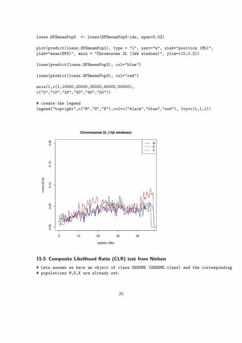
plot(predict(loess.SFSmeanPop1), type = "l", xaxt="n", xlab="position (Mb)",ylab="mean(SFS)", main = "Chromosome 2L (1kb windows)", ylim=c(0,0.2))
lines(predict(loess.SFSmeanPop2), col="blue")
lines(predict(loess.SFSmeanPop3), col="red")
axis(1,c(1,10000,20000,30000,40000,50000),c("0","10","20","30","40","50"))
# create the legendlegend("topright",c("M","S","X"),col=c("black","blue","red"), lty=c(1,1,1))
15.5 Composite Likelihood Ratio (CLR) test from Nielsen# Lets assume we have an object of class GENOME (GENOME.class) and the corresponding# populations M,S,X are already set.
25

# Lets apply the CLR test on genes and define a global set of the SFS# based on all Coding SNPs
# extract the genomic positions of the genes out of the corresponding GFF filegenes <- get_gff_info(gff.file="twoL.gff",chr="2L", feature="genes")
# splitting the data into gene regions# type=2 have to be set because the values are genomic positionssplit <- splitting.data(GENOME.class, positions=genes, type=2)
# calculate the minor allele frequenciessplit <- detail.stats(split)
# extract the minor allele frequencies from all gene regions for each populationfreqM <- sapply([email protected]@minor.allele.freqs,function(x){return(x[1,])})freqS <- sapply([email protected]@minor.allele.freqs,function(x){return(x[2,])})freqX <- sapply([email protected]@minor.allele.freqs,function(x){return(x[3,])})
# Create the global frequencies table which are neccessary for the CLR test.freqM <- table(unlist(freqM))freqS <- table(unlist(freqS))freqX <- table(unlist(freqX))
# Now, lets calculate the CLR test using the module sweeps.stats
split <- sweeps.stats(split, freq.table=list(freqM,freqS,freqX))
head(split@CLR)
pop 1 pop 2 pop 3[1,] 126.53772 187.70825 316.40969[2,] 10.93362 13.37492 34.85426[3,] 22.07749 25.43857 42.07533[4,] NA NA NA[5,] 10.93362 13.11267 16.18083[6,] 254.16225 303.04791 352.00897
15.6 Mcdonald-Kreitman test# Read in the data with the corresponding GFF fileGENOME.class <- readVCF("twoL.vcf.gz",15000,"2L",1,50000000,include.unknown=TRUE, gffpath="twoL.gff")
26

# Verify the syn/non-syn SNPsGENOME.class <- set.synnonsyn(GENOME.class, ref.chr="twoL.fas")# Set the populationsGENOME.class <- set.populations(GENOME.class, list(M,S,X), diploid=TRUE)# Splitting the data into genessplit <- splitting.data(GENOME.class, subsites="gene")
# Peform the MKTsplit <- MKT(split)
# To look at gene 9 we can do the following:split@MKT[[9]]
P_nonsyn P_syn D_nonsyn D_syn neutrality.index alphapop1/pop2 3 2 0 0 NaN NaNpop1/pop3 7 2 5 4 2.8 -1.8pop2/pop3 6 2 5 4 2.4 -1.4
# or alternativelyget.MKT(split)[[9]]
16 Graphical output: R package ggplot216.1 Creating data.framesLets assume we have transformed the data into sliding windows or specific regions andalready performed the Fixation index FST. To create an compact data representationof the most informative values we could do the following:
# Extracts the information stored in the slot region.names# and converts the strings to numeric values (start position of the# region and end position)
from.pos <- sapply([email protected],function(x){return(as.numeric(strsplit(x," ")[[1]][1]))})
to.pos <- sapply([email protected],function(x){return(as.numeric(strsplit(x," ")[[1]][3]))})
# Lets concatenate the values into a matrixDATA <- cbind(from.pos, to.pos, [email protected]_ST)
27

# Converting into a data.frameDATA <- as.data.frame(DATA)
The native R function sapply is a very performant approach to extract values also storedin the region.data or region.stats slots where data is mostly organized as lists.
17 Performing readVCF in parallelTo accelerate computations for the readVCF function the mechanism provided by thefunction mclapply from the package parallel might be a good option. readVCF canbe applied to different regions of the VCF file so that we can contribute the readingprocess on different nodes. The returned object is a list of classes from the type GENOME.Note, the ff-package which is used for storing whole genome variation data is limitedby n.individuals * n.snps <= Maschine$integer.max. If the data is bigger thanthat the bigmemory package will be applied. The corresponding access function aremuch slower than those provided by the ff-package. As an example we read in data viareadVCF from the region 1-10.000.000, but parallize the reading process on two nodes.(1-5.000.000 and 5.000.001-10.000.000).
# Loading the R-package parallelrequire(parallel)
# Lets define the two regions
cregions <- character(2)cregions[1] <- "1-5000000"cregions[2] <- "5000001-10000000"
GENOME.classes <- parallel::mclapply(as.list(cregions),
function(x){
From <- as.numeric(strsplit(x,"-")[[1]][1])To <- as.numeric(strsplit(x,"-")[[1]][2])
return(readVCF(filename="AGC_refHC_bialSNP_AC2_2DPGQ.2L_V2.CHRcode2.vcf.gz",numcols=1000, tid="2", frompos=From, topos=To, samplenames=NA,gffpath=FALSE, include.unknown=TRUE,approx=FALSE, out=x, parallel=FALSE))},
mc.cores = 2, mc.silent = TRUE, mc.preschedule = TRUE)
28

> GENOME.classes[[1]]@region.names[1] "2 : 1 - 5000000"> GENOME.classes[[2]]@region.names[1] "2 : 5000001 - 10000000"
The splitted classes can now be used seperately.
slide <- sliding.window.transform(GENOME.classes[[1]],1000,1000)slide <- diversity.stats(slide)
Also we can concatenate those classes:GENOME.class <- concatenate.classes(GENOME.classes)GENOME.class <- concatenate.regions(GENOME.class)
18 Pre-filtering VCF files18.1 VCF tools
18.2 WhopGenome
29


