Whntn - Yakima Basin Fish and Wildlife Recovery Board · Whntn prtnt f IS nd WIIE thd fr pln th...

WashingtonDepartment of

FISH andWILDLIFE

Methods for Sampling the Distribution and Abundanceof Bull Trout and Dolly Varden

by

Scott A. Bonar, Marc Divens, and Bruce BoldingInland Fisheries InvestigationsResources Assessment Division

Washington Department of Fish and Wildlife600 Capitol Way NorthOlympia, WA 98516

June, 1997

ABSTRACT

We compared methods for determining the distribution and abundance of bull trout Salvelinusconfluentus and Dolly Varden Salvelinus malma. For detecting the presence of adult andjuvenile bull trout/Dolly Varden, night snorkeling was the most effective technique followed byelectrofishing and angling/foot surveys. We recommend first conducting informal surveys usingangling, day snorkeling, night snorkeling and/or night bank walking in preferred bull troutspawning or initial rearing habitat within a patch. We define "patch" as a stream reach or groupof reaches separated from others by thermal or geographic barriers to their migration. If no bulltrout/Dolly Varden are found, and if a specified degree of confidence is wanted for lowerdetection limits, a statistically rigorous survey is needed. To be 95 percent confident that bulltrout/Dolly Varden are in densities less than 0.60 fish/100 m (assuming a minimum samplingefficiency of 25 percent), snorkel or electrofish, using the guidelines in this report, 20 randomlychosen 100 m sections of preferred habitat within the patch. Sample 11 randomly chosensections to be 80 percent confident. Sampling requirements for other combinations of densities,sampling efficiencies and confidence intervals are also provided in this report.

Redd surveys and traps are preferred methods for estimating total adult abundance andescapement. Redd surveys are suitable for both migratory and resident populations, while trapsbest monitor migrating fish. Obtain cumulative redd counts in a system by surveying the entirespawning habitat, or by random sampling of the habitat, depending on the accuracy and precisiondesired. Cumulative counts can be multiplied by 2.2, an average spawner:redd ratio for sevenPacific Northwest watersheds, or preferably a spawner:redd estimate for that particular system toobtain total escapement.

Methods for Sampling the Distribution and Abundance of Bull Trout and Dolly Vardenii

TABLE OF CONTENTS

LIST OF TABLES

LIST OF APPENDIXES vi

ACKNOWLEDGMENTS vii

INTRODUCTION 1

METHODS 3Distribution 3Abundance 3Sampling Method Selection 4

RESULTS AND DISCUSSION 5Distribution Surveys 5

Comparison of Distribution Survey Methods 5Techniques for Conducting Night Snorkeling Surveys 6Distribution Survey Design 7

Delineation of Survey Area Boundaries 7Surveying the Patch 8

The Informal Survey 9The Statistical Survey 9

Abundance And Escapement Surveys 13Methods to Measure Abundance 13

Juvenile Abundance 13Adult Abundance 14Redd Counts 14Monitoring Abundance Under Conditions of Low Water Visibility and

Redd Superimposition 17Abundance Survey Design 18

Prioritizing and Selecting Sampling Sites 18Types of Survey Designs 19

Index Areas 19Trap or Fence Counts of Adults 20Surveying an Entire Stream or Watershed 20Random Sampling of Redds Within a Watershed 20

Calculating Spawner Escapement 27Estimating Escapement and Associated Confidence Intervals Using Redd

Counts 27Estimating Escapement 27

Methods for Sampling the Distribution and Abundance of Bull Trout and Dolly Vardeniii

Estimate of Variance for Escapement 28Confidence Intervals for Total Escapement Estimates 29

Using Snorkeling Counts of Adults to Estimate Escapement 30Considerations When Evaluating The Status of Bull Trout Populations 31

CONCLUSIONS 32

REFERENCES 39

Methods for Sampling the Distribution and Abundance of Bull Trout and Dolly Vardeniv

LIST OF TABLES

Table 1. Comparison of methods used to enumerate bull trout 33

Table 2. Comparison of methods for determining distribution of bull trout in Washington streamsand rivers, fall 1995 34

Table 3. Densities of juvenile bull trout encountered (e) by night snorkeling in Pacific Northweststreams and rivers 35

Table 4. Ratio of number of bull trout spawners to redds in various Pacific Northwest rivers 36

Table 5. Key to help select appropriate method for sampling bull trout 37

Methods for Sampling the Distribution and Abundance of Bull Trout and Dolly Varden

LIST OF APPENDIXES

Appendix 1. Stream electrofishing guidelines for Washington Department of Fish and Wildlifedistribution (stream typing) surveys 45

Appendix 2. Encounter densities (c) and number of 100m stream sections (n) to be surveyed fordetecting bull trout with 95 percent confidence at a variety of sampling efficiencies andmean densities 47

Methods for Sampling the Distribution and Abundance of Bull Trout and Dolly Vardenvi

ACKNOWLEDGMENTS

We thank Washington Department of Fish and Wildlife biologists and management staff forproviding us with a considerable amount of information and allowing us to participate in selectedbull trout surveys. We especially thank Eric Anderson, Larry Brown, Dan Collins,Jim Cummins, Bob Gibbons, Joe Foster, Doug Fletcher, Bill Freymond, Jim Johnston,Curt Kraemer, Paul Mongillo, Chuck Phillips, Bob Pfeifer, John Weinheimer and Ken Williams.Paul James and students of Central Washington University; Steve Thiesfeld, Steve Pribyl andMary Hanson of Oregon Department of Fish and Wildlife; Joseph Bonneau and George LaBarof the University of Idaho; Delbert Skeesick of the U.S.D.A. Forest Service (Retired) alsoprovided information for our study. Steve Jackson suggested the key format for managementrecommendations.

The following reviewed our study and provided valuable comments and suggestions:Jim Capurso and others of the U.S. Forest Service; Steve Elle of the Idaho Department of Fishand Game; Bruce Rieman of the U.S. Forest Service Intermountain Research Station;Shelly Spalding of Montana Fish Wildlife and Parks; Barbara Kelly and others of the U.S. Fishand Wildlife Service; Eric Anderson, Larry Brown, Craig Burley, Jim Cummins, Ray Duff,Peter Hahn, Jim Johnston, Curt Kraemer, Paul Mongillo, Ken Williams and William Zook of theWashington Department of Fish and Wildlife. Terry Jackson provided the stream electrofishingguidelines in Appendix 1.

We especially thank Colleen Desselle and Kay Bujacich-Smith, who provided considerableadministrative and graphical support.

Methods for Sampling the Distribution and Abundance of Bull Trout and Dolly Vardenvii

INTRODUCTION

Bull trout Salvelinus confluentus populations have declined in many parts of their range (Riemanand McIntyre 1993) and recently, the U. S. Fish and Wildlife Service confirmed that Klamathand Columbia River bull trout population segments warranted listing under the FederalEndangered Species Act. Several management actions have been recommended or initiated toprotect bull trout populations such as angling restrictions (Fraley et al. 1989, Anon 1995a, Anon1995b,), habitat protection (Fraley et al. 1989, Brown 1992, Anon 1995b) and reducing theirinteractions with exotic fish (Buckman et al. 1992, Dambacher et al. 1992).

Until recently, all native char in Washington were called Dolly Varden S. malma. AfterCavender's 1978 recognition of the bull trout as a species separate from Dolly Varden, there hasbeen considerable confusion in separating the two. In Washington, these species are commonlymanaged together, sampled using the same techniques, and stocks of both are considered"vulnerable" (Brown 1994). Therefore, for the purposes of this report, we use "bull trout" torefer to either Dolly Varden or bull trout.

Monitoring the distribution and abundance of bull trout is necessary to determine the status ofvarious populations, factors associated with their relative health, and if management actionsinitiated to rebuild depressed populations are working. Monitoring distribution and abundancecan also identify populations and areas that should receive high levels of protection.

A variety of methods are currently used to measure bull trout populations. Range or distributionof this species has been examined using general stream fisheries survey methodology such asangling and streamside foot surveys (Johnson and Shrier 1989), electrofishing (Fraley andShepard 1989, Schill 1991, Rieman and McIntyre 1995), and snorkeling (Hillman and Platts1993, Bonneau et al. 1995, Rieman and McIntyre 1995). Bull trout abundance has beendetermined using redd counts (Fraley and Shepard 1989, Brown 1992), trap counts (Fraley andShepard 1989), snorkeling counts (Goetz 1991, Sexauer and James 1993), creel surveys (Fraleyand Shepard 1989), and mark and recapture estimates (Faler 1995).

It is estimated that Washington currently has 80 distinct stocks of bull trout/Dolly Varden. For 62of these stocks, there is currently not enough information about their population status to assigna level of risk (Washington Department of Fish and Wildlife 1996). Management biologists arecurrently surveying populations, and need effective monitoring protocols.

The purpose of our study was to:1) identify those methods currently being used to monitor bull trout distribution and

abundance;

2) examine the precision and accuracy of these techniques;

3) determine the suitability of existing methods for monitoring bull trout populations inWashington and recommend modifications or new methods if needed;

Methods for Sampling the Distribution and Abundance of Bull Trout and Dolly Varden1

4) recommend standardized survey methods for bull trout abundance and distribution forthe Washington State Department of Fish and Wildlife; and

5) develop a dichotomous key to aid in selecting suitable sampling methods.

Our report only examines methods for sampling bull trout populations, and does not describeassociated habitat survey methods. However, habitat change can impact bull trout populationsand those interested in monitoring habitat can consult Brown (1992) and Shepard and Graham(1983).

We describe a variety of methods used to survey bull trout, and the reader should not feel thatevery listed method should be applied with the highest degree of statistical rigor for all surveys.Rather pros and cons of various survey options are described, the authors' recommendations aregiven, and the task of choosing the most appropriate method is left up to the reader.


METHODS

Distribution

Several methods are available for monitoring distribution of bull trout. The ideal survey methodwould:

1) have a high capture or encounter rate,

2) be cost—effective for use in remote areas,

3) not harm bull trout populations, and

4) be safe to conduct.

We examined the characteristics of four methods for determining bull trout distribution: anglingand foot surveys; night snorkeling; day snorkeling and electrofishing. Information was obtainedthrough publications and technical reports, contacts with Pacific Northwest fisheriesmanagement biologists, and comparisons of these techniques in selected Eastern and WesternWashington streams and rivers.

The most efficient technique for determining the presence of a species will have the highestprobability of encountering individuals. Therefore, we compared the number of fish enumeratedusing each method to indicate which technique would most likely find bull trout in areas wherethey were sparsely distributed. In the North Fork Skokomish River above Staircase Rapids, weangled and foot surveyed a 1.9 km section during the day on October 24, 1995, when bull troutwere spawning, and then snorkeled the same section during the day and at night on October 26,1995, recording total numbers of both juvenile and adult bull trout. We conducted a similarday—night snorkel comparison of bull trout abundance in the 2.1 km section of the North ForkSkokomish River below Staircase Rapids on October 28, 1995. We compared day snorkeling toangling techniques combined with foot surveys during September 25-27, 1995, in severalsections of the Waptus River basin. On Rattlesnake Creek, day snorkeling was compared toangling in a 0.3 km section of creek and night snorkeling was compared to angling in a 0.15 kmsection during September 11-13, 1995.

Abundance

We evaluated redd counts, adult counts by trapping and day and night snorkeling, and juvenilecounts by day and night snorkeling and electrofishing to determine which were the most accurateand cost—effective methods to measure abundance. To compare methods, we examinedpublications, technical reports and data sets obtained from western states and Canadian provincescontaining bull trout populations. We also accompanied WDFW management biologists onabundance surveys during the 1995 spawning season at Merwin Reservoir, the North ForkSkokomish River, the North Fork Skykomish River and the South Fork Sauk River.

Methods for Sampling the Distribution and Abundance of Bull Trout and Dolly warden3

Sampling Method Selection

After compiling information from both field and literature data, we developed a dicotomous keyto aid surveyors in identifying appropriate sampling methods for both distribution and abundancesurveys. The key was designed to help select methods based on the survey objectives and theenvironmental conditions of the survey area.


RESULTS AND DISCUSSION

Distribution Surveys

Comparison of Distribution Survey Methods

Most sources, including our field surveys, found night snorkeling had the highest or was tied forthe highest encounter rate for juvenile bull trout (Tables 1 and 2). This was followed in order byangler and foot surveys, electrofishing, and day snorkeling. The efficiency of angler and footsurveys may have been overestimated because of the few studies evaluating this procedure. Daysnorkeling was generally the least effective technique, except when water temperatures were over9° C (Thurow and Schill 1996). Juvenile bull trout hide in the substrate during the day,especially in the presence of other fish species (Goetz 1991) or when water temperatures fallbelow 9°C (Thurow 1997).

Our results using night snorkeling for encountering adult bull trout were different than those ofother researchers. Goetz (1991) found that night snorkeling was the most effective technique forencountering age 2+ fish (> 125 mm); however, we counted more adult bull trout (> 450 mm)during the day on the Skokomish River than on our night snorkeling trip (Table 2). We noticedadult bull trout avoiding our lights as we traveled downstream in this large river, which may havecontributed to the night count being lower than the day count. Future surveys incorporatinglow—powered lights may reduce the avoidance of the adult fish in large rivers when snorkelsurveys downstream are necessary.

We did not examine the suitability of the various methods for determining the presence of bulltrout fry, however Goetz (1991) found that night snorkeling underestimated fry abundancecompared to other methods since at night juveniles emerge and fry tend to seek cover.

Since most studies have found night snorkeling to have the highest encounter rate with adult andjuvenile bull trout, we recommend night snorkeling as the preferred method for distributionsurveys. However, in some remote areas, night snorkeling or night foot surveys can beinappropriate because of safety concerns. Therefore, other techniques may be useful in thesesituations. Day snorkeling counts are efficient in some Pacific Northwest streams during thesummer. The efficiency of day snorkeling counts approached night snorkeling counts whenwater temperatures were above 9°C in an Idaho study (Thurow and Schill 1996). This mayreflect changes in diel habitat use by bull trout over the year. In summer, juvenile bull trout maybe more likely to be in the water column during the day than in the winter. In winter surveys ofProfile Creek, Idaho, bull trout commonly sought cover during the day and moved into the watercolumn at night (Thurow 1997). It is unknown how close summer night and day counts areunder a variety of stream flow conditions, habitat types, and existing fish communities.Although day counts can approach night counts when water temperatures are over 9°C, we found


no studies where day counts were consistently higher than night counts. Therefore, whenconditions are suitable, night surveys should be employed.

Electrofishing has proven effective for capturing bull trout in small streams (Shepard andGraham 1983, Schill 1991, Thurow and Schill 1996), especially those with adequate conductivity(approaching 100 µS/cm). However, this technique may be harmful to fish or fish eggs (Schrecket al. 1976, Sharber and Carothers 1988, Fredenberg 1992, Dwyer and Erdahl 1995). Since bulltrout are currently warranted for listing as threatened or endangered, any technique which couldresult in their injury should be carefully considered before it is selected for use. Many streamscurrently being investigated with distributional surveys are located in remote areas which aredifficult to reach carrying electrofishing equipment. Carrying snorkeling equipment can belaborious, but less so than transporting electrofishing units. Because of these concerns, werecommend electrofishing be avoided when possible. If electrofishing use is required (e.g.,streams too shallow to snorkel), only highly trained personnel should be allowed to operateequipment at settings designed to minimize injury to fish. The Washington Department of Fishand Wildlife has developed draft electrofishing guidelines for salmonid distribution surveys(Appendix 1).

For distribution surveys, we recommend using night snorkeling where possible. Daysnorkeling can be effective in waters > 9°C. Electrofishing can be effective in sites withadequate conductivity (approaching 100 µS/cm), but should be avoided if possiblewhere potential injury to fish is of concern.

Techniques for Conducting Night Snorkeling Surveys

Proper equipment and adequate precautions are necessary to ensure a safe, effective nightsnorkeling survey. Thurow (1994) and Bonneau et al. (1995) discuss snorkeling surveyequipment and techniques in detail. We packed both wet suits and dry suits into remote areas,and found that for ease of transport and warmth in cold rivers, dry suits were preferable. In areaswhere considerable streamside walking is required, and overheating is a problem, wet suits canbe useful. Wet suits also cushion the impact with rocks in the stream. Surveyors may want totest both types of suits before purchasing. Thurow (1994) recommends dark colored nylondrysuits over neoprene, purchased without valves and with attached latex socks. We found thatmetal studded wading boots, worn over neoprene booties or socks, allowed us to move safely andrapidly over slick rocks and downed timber. Data can be recorded on a cuff made from PVC(Thurow 1994) or by a shore observer.


We used three types of lights for our surveys: large lights (7-14 watts) made for SCUBA divingsuch as UK 600 or UK 1200s', small SCUBA lights (4-6 watts), and small waterproof flashlightsreadily available at hardware stores. We found small SCUBA lights worked best, since largeSCUBA lights frightened fish, and the waterproof hardware flashlights did not provide enoughlight and their battery life was extremely short in the cold water. Because of their short life incold water, many spare batteries should be carried on night surveys by the shore observer(Bonneau 1995). Hillman (1993, cited in Thurow 1994) found that most salmonid species wouldmaintain their position longer if filters made from red Plexiglass were used on lights.

Night snorkeling safety is an important concern for a survey crew. This technique should beavoided in rapids and log—jammed sections of larger creeks and rivers which might be snorkeledor angled during the day. Most small tributaries can be snorkeled during nighttime, and in thesesystems, survey crews should move upstream to minimize scaring fish which usually faceupstream (Thurow 1994). For snorkeling larger systems at night such as the North ForkSkokomish River, Washington, we moved downstream, and used considerable care to ensure asafe survey. On this river, we scouted the area to be snorkeled during the day to identify thepools and glides we wanted to snorkel and hazardous areas we should avoid. We neversnorkeled at night through rapids or where moving water flowed close to log jams. One teammember snorkeled while an observer remained on shore in snorkeling gear, ready to enter thewater if problems arose. Two snorkelers, in addition to the shore observer, would have beenpreferable to one. The snorkeler entered the water at the top of a pool or glide deemed safe andmoved downstream. The shore observer stood at the bottom of glides and pools with a light,signaling where the snorkeler should stop. The snorkeler also covered small side channels ortributaries. Even though we did not cover all of the available bull trout habitat on the upperSkokomish River, and used half the effort that we did in the day (1 snorkeler vs. 2), we saw bulltrout at night, while we did not during our day snorkeling or angling surveys.

In certain areas, night snorkeling may be too hazardous to conduct. If conditions dictate that daysnorkeling be used, conduct surveys when water temperatures are above 9°C, and ensure thatin—stream cover, such as beneath rocks and woody debris, is thoroughly searched.

Distribution Survey Design

Delineation of Survey Area Boundaries

Bull trout are particularly sensitive to angling pressure and environmental degradation (McPhailand Baxter 1996). Angling pressure on Washington bull trout populations has been considerablyreduced through restrictive regulations. Therefore, limiting factors for healthy bull troutpopulations are likely spawning and juvenile rearing habitat (McPhail and Murray 1979, cited in

1 Mention of a vendor does not constitute endorsement.


Brown 1994; Mullan et al. 1992). Since identification and protection of these sites is essential topreserve populations, presence/absence surveys should be concentrated first in stream or riverreaches where the potential exists for this type of habitat. Waters which might contain bull trout,but do not contain critical spawning and rearing habitat include coastal lowland rivers where bulltrout occasionally enter to feed; stream and river sections through which adults and juvenilesmigrate to reach spawning or rearing areas, lakes, or the ocean. While life history informationcan be collected from these sites, it is probably not of high priority to survey them immediatelyfor presence/absence.

Once watersheds are identified that contain suitable spawning or rearing habitat, areas to besurveyed must be delineated within them. Protection of subpopulations of bull trout increasesthe resilience of the species to extinction (Rieman and McIntyre 1993). The presence of severalsubpopulations increases the probability that at least one will survive periods of disturbance.Additionally, genetic interchange between subpopulations increases their fitness. Detecting thepresence of distinct bull trout subpopulations and protecting them is the key to halting the declineof the bull trout (Rieman and McIntyre 1993).

Subpopulations often form in individual streams or groups of streams containing suitablespawning or initial rearing habitat which are separated from others by geographic or thermalbarriers to migration (Rieman and McIntyre 1993, Rieman and McIntyre 1995). Presence of bulltrout in these areas or "patches" (Rieman and McIntyre 1995) could indicate distinctsubpopulations. Therefore, for determining presence of a possible subpopulation, we define thesurvey section of interest as a patch which is bordered by barriers to migration. Although bulltrout can move between patches, at least some reproductive isolation occurs. Barriers tomigration can include long reaches of unsuitable habitat, waterfalls, large cascades, lakes, theocean, headwaters or downstream thermal barriers. Once presence of bull trout in a patch isestablished, genetic testing can then be used to evaluate the degree of relationship between bulltrout within or among patches.

We define the area of interest or "patch" for establishing presence of bull trout as astream reach or group of streams which contains suitable spawning or initial rearinghabitat and is separated from other patches by barriers to migration.

Surveying the Patch

After the patch is identified, it can be surveyed using the following recommendations.

We recommend that survey of the patch be conducted in two stages: (1) first aninformal survey where presence of bull trout may be established with minimal effort;and then (2) if no fish are found and if non—detection limits are required with a certainlevel of confidence, a more intense statistically rigorous survey should be conducted.


The Informal Survey: To conduct the informal survey, we recommend that the surveyor walk,angle, and/or day or night snorkel some of the potential preferred habitat within the section.Surveyors should especially look close to barriers, such as a pool beneath a large rapids orwaterfall. Conducting surveys during the fall spawning season will give the maximum chance ofencountering migrating spawners. Juvenile abundance can fluctuate throughout the year. Bestresults can be obtained by surveying at different times, and if conducting daytime surveys,waiting until water temperatures are above 9°C. Bonneau et al. (1995) found that walking atnight along the shallow margins of the stream and backwater areas was effective for recordingthe presence of juvenile bull trout.

Preferred habitat for bull trout spawning and rearing has been discussed in detail elsewhere(Fraley and Shepard 1989, Mullan et al. 1992, Sexauer and James 1993, Brown 1994, McPhailand Baxter 1996), and includes lengths of streams containing pocket pools, side channels, areasof ground water upwelling, woody debris, suitable water temperatures, suitable substratecomposition and areas at the base and head of rapids. We define "preferred habitat" not as theindividual microhabitats such as pocket pools or downed logs, but a reach of stream whichcontains a substantial amount of these microhabitats. Length and location of preferred habitatsections should be recorded on a detailed map of the patch on this initial survey, either by GPScoordinates or estimates of the surveyor. If it is decided later that absence should be determinedwith a specified degree of confidence, then the map of preferred habitat data is available fromwhich to randomly sample.

If individuals are observed, presence is established. If individuals are not observed, randomsampling and statistical rigor is necessary for determining that bull trout are non—detectible.

The Statistical Survey: Informal surveys may be sufficient to determine general bull troutdistribution in an area. However, a statistically rigorous survey is needed to determine if bulltrout are present where the potential exists for impact from development, logging, or roadbuilding to areas which contain preferred bull trout habitat or to the headwaters above preferredhabitat. In these situations, it is important that there is a specified degree of confidence that bulltrout are non—detectable.

First, the map of the patch developed in the informal survey should be used to identify locationsof preferred spawning and initial rearing habitat. Sampling sites should then be randomly chosenfrom the preferred habitat, using the statistical procedures that follow, to maximize the chance ofencountering bull trout. If the entire patch is preferred habitat, then samples should be randomlyallocated over the entire patch.

Hillman and Platts (1993) developed a bull trout survey methodology that incorporates randomsampling of stream sections using day snorkeling and electrofishing. To detect the presence ofbull trout with a specified degree of power, they used a sampling technique developed by Greenand Young (1993) which considers the distribution of any rare species (density < 0.4 per


sampling unit) to fit the Poisson distribution. They reported that the number of samples n (i.e.,stream sections or quadrats) required to detect a rare species with a specified power (1 - p) is

In/ (1)n = -

m

where m = the mean density of the rare species. This procedure assumes that all bull troutpresent are detected, i.e., sampling efficiency is 100 percent. However, for bull trout, samplingefficiency can range from 20 percent to 90 percent depending on time of year and samplingtechniques, but rarely approaches 100 percent (B. Rieman 1997). Rieman and McIntyre (1995)assumed a minimum sampling efficiency of 25 percent for their work, and we adopted it for oursampling protocol. Correcting (1) to account for our assumption that only 25 percent of the bulltrout present are detected, the number of samples required to encounter bull trout is

n - - lnfi ln fi

(2)(0.25)m

Where e = density of bull trout encountered (e.g., sampling efficiency x mean density m). Forpower 143 = 0.95, or for power 1-13 = 0.80 these equations reduce to simple relationships.

The necessary number of 100 m stream sections to survey for a 95 percent chance ofdetecting bull trout in a patch, assuming a minimum detection efficiency of 25 percent,is equal to

n3 3 12- (3) E (0.25)m

where m = the mean density of bull trout in fish per 100 m, ande = density of bull trout encountered per 100 m


The necessary number of 100 m stream sections to survey for an 80 percent chance ofdetecting bull trout in a patch, assuming a minimum sampling efficiency of 25 percent,is equal to

1.6 1.6 6.4 (4)n - —

(0.25)m

Where m = the mean density of bull trout in fish per 100 m, ande = density of bull trout encountered per 100 m

Mean encounter densities (c) reported for night snorkeling in bull trout spawning and rearinghabitat range from 0.26 to 42.5 fish/100 m (Table 3). During day snorkeling surveys, es were aslow as 0.15 fish/100 m in Icicle Creek and 0.14 fish/100 m in Jack Creek, Washington (Kelly1997). In these surveys, sampling efficiency may have approached that of night snorkeling,since counts were made during the summer when water temperatures were above 9°C. Werecommend that these lowest encounter densities, rounded for ease of use to 0.15, be consideredas the threshold for "non—detectable." This corresponds to an actual density of 0.60 fish/100m,assuming a sampling efficiency of 25 percent. When presenting survey results, we recommendstating that bull trout were non—detectable, or in densities less than 0.60 fish/100m as opposed to"absent."

A lower threshold for detection of c = 0.15 fish/100m is conservative compared to that used byothers. Hillman and Platts (1993) recommended that 0.25 fish/100 m using day snorkeling andelectrofishing be used, and 0.25 fish/100 m was recommended as a lower threshold at aworkshop for bull trout sampling techniques coordinated by the Forest Service (Harkenrider1994). Rieman and McIntyre (1995) assumed that bull trout in densities less than 1.5 fish/100 m(c = 0.37 fish/100 m, assuming a sampling efficiency of 25 percent) would be at high risk ofextinction through demographic stochasticity, Allee effects or other small population effects.

Substituting 0.15 fish/100m in Equations (2) and (3) for e will give the number of sampling sitesneeded for both the 80 percent and 95 percent levels of confidence.


Night snorkel (preferred method), day snorkel at water temperatures over 9°C, orelectrofish twenty 100 m long randomly selected sections of preferred habitat in apatch to have a 95 percent chance of sighting bull trout when they are at an actualdensity (m) of 0.60 fish/100 m in preferred habitat of stream, assuming a minimumsampling efficiency of 25 percent;

To have an 80 percent chance of detecting bull trout at the same mean density, eleven100 m long randomly selected sections of preferred habitat must be sampled in a patch.

The sampling efficiency of electrofishing a stream with adequate conductivity (approaching 100gS/cm), or day snorkeling when water temperatures are over 9°C, has consistently exceeded 25percent in other studies (Rieman and McIntyre 1995). The sampling efficiency of nightsnorkeling is usually higher than either of these two methods (Table 1). Any one of these threetechniques will probably be adequate for surveying a patch for presence/absence with theconfidence stated above. The advantage of using night snorkeling is that fish are likely to beencountered more rapidly in the patch, so less effort will have to be expended per survey if bulltrout are present. Also night snorkeling will be more powerful than the other two methods fordetecting bull trout if they occur at densities less than 0.60 fish/100 m. If future studiesdetermine the actual minimum sampling efficiency of night snorkeling, the required sample sizefor detecting bull trout using night snorkeling could be reduced. Consult Appendix 2 to calculatesample sizes assuming other minimum sampling efficiencies or mean densities.

Upon examination of Equation (1), patch size does not have any impact on required samplesize. If larger patches receive more sampling effort than smaller ones, the probability of findinga bull trout is positively biased towards the larger patches. To sample a 30 km preferred habitatsection of stream, assuming "presence" is defined as encountering more than 0.15 fish/100 m,would require 20 samples for a 95 percent chance of encountering a bull trout. A 10 kmpreferred habitat section with the same mean density would require the same number of samples(20) to encounter the fish. This sample size is appropriate even if bull trout are present inaggregated (clumped, patchy) distributions, since aggregated distributions approach the Poissonas bull trout abundance becomes rare (m < 0.40)(Green and Young 1993).

Example 1. Designing a Distribution (Presence/Absence) Survey

The Waptus River is medium—sized and flows from Lake Ivanhoe to Waptus Lake to theCle Elum River. Between the outlet from Waptus Lake and the Cle Elum River, there is a largewaterfall, Pamlaur Falls. A biologist is interested to determine if there are bull trout in themainstem Waptus above Pamlaur Falls. There are two "between—barrier" patches in this reach ofriver. One is the roughly 12.9 km section upstream of the falls to Waptus Lake. The other is the4.8 km section from Waptus Lake to Lake Ivanhoe.


12

The Informal Survey: First the biologist walks, angles, and does some night or day snorkelingfocusing on preferred habitat in both these areas. At the same time he notes that the entire riverabove the falls, except for a 1.2 km section above Waptus Lake, consists of preferred bull troutspawning and rearing habitat, and records this on a map. He finds no bull trout during thissurvey.

The Statistical Survey: The next year, there is interest to determine if bull trout are absent, thatis at densities < 0.60 fish per 100 m, with a 95 percent degree of confidence. A team ofbiologists randomly selects 20-100 m sections to snorkel in the 3.6 km reach of preferred habitatabove Waptus Lake and 20-100 m sections in the 12.9 km reach from Waptus lake to PamlaurFalls. When they get to the lake, they decide to night snorkel the entire 3.6 km upper reachbecause it is easier than breaking up the river into sections. In the lower reach, they noticeduring the day, one of the randomly chosen 100 m sections runs through a potentially dangerouscanyon. This is excluded from the survey, another section is randomly chosen outside thecanyon, and the survey conducted. No bull trout are seen in either of the reaches, and thebiologist now knows there is a 95 percent chance that bull trout are in densities less than 0.60fish per 100 m in each reach of the Waptus River above Pamlaur Falls.

Abundance And Escapement Surveys

Changes in the abundance of bull trout in a stream, watershed, or statewide, as well ascontractions or expansions in range, can signal the necessity of stringent management plans ifpopulations are declining, or demonstrate the success of management actions if populations areincreasing. Before abundance surveys are conducted, a clear objective of the purpose of thestudy is needed. A statement of study objectives is often overlooked, but is of primaryimportance since it will dictate what methods are to be used. For instance, if evaluating thesuccess of recent reproduction is important, measurement of juvenile densities may be better thanadult counts. If total escapement or the number of spawners is important, either redd or trapcounts can supply the needed information.

Methods to Measure Abundance

The abundance of each life—history stage of bull trout can be monitored using a variety oftechniques. Many of the following surveys should be conducted several times during the seasonof interest.

Juvenile Abundance

Juvenile abundance is a measure of the success of more recent reproduction than adult counts,and may provide important early indications of habitat problems (Weaver and Fraley 1991) orimpacts of non—native fish. Additionally, juvenile counts do not have to be restricted specificallyto the spawning season. However, juvenile counts made in the same section of stream can be


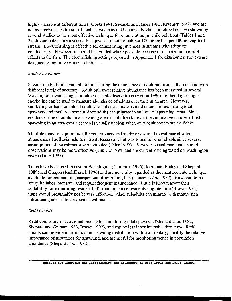
highly variable at different times (Goetz 1991, Sexauer and James 1993, Kraemer 1996), and arenot as precise an estimator of total spawners as redd counts. Night snorkeling has been shown byseveral studies as the most effective technique for enumerating juvenile bull trout (Tables 1 and2). Juvenile densities are usually expressed in either fish per 100 m 2 or fish per 100 m length ofstream. Electrofishing is effective for enumerating juveniles in streams with adequateconductivity. However, it should be avoided where possible because of its potential harmfuleffects to the fish. The electrofishing settings reported in Appendix 1 for distribution surveys aredesigned to minimize injury to fish.

Adult Abundance

Several methods are available for measuring the abundance of adult bull trout, all associated withdifferent levels of accuracy. Adult bull trout relative abundance has been measured in severalWashington rivers using snorkeling or bank observations (Annon 1996). Either day or nightsnorkeling can be used to measure abundance of adults over time in an area. However,snorkeling or bank counts of adults are not as accurate as redd counts for estimating totalspawners and total escapement since adults can migrate in and out of spawning areas. Sinceresidence time of adults in a spawning area is not often known, the cumulative number of fishspawning in an area over a season is usually unclear when only adult counts are available.

Multiple mark—recapture by gill nets, trap nets and angling was used to estimate absoluteabundance of adfluvial adults in Swift Reservoir, but was found to be unreliable since severalassumptions of the estimator were violated (Faler 1995). However, visual mark and snorkelobservations may be more effective (Thurow 1994) and are currently being tested on Washingtonrivers (Faler 1995).

Traps have been used in eastern Washington (Cummins 1995), Montana (Fraley and Shepard1989) and Oregon (Ratliff et al. 1996) and are generally regarded as the most accurate techniqueavailable for enumerating escapement of migrating fish (Cousens et al. 1982). However, trapsare quite labor intensive, and require frequent maintenance. Little is known about theirsuitability for monitoring resident bull trout, but since residents migrate little (Brown 1994),traps would presumably not be very effective. Also, subadults can migrate with mature fishintroducing error into escapement estimates.

Redd Counts

Redd counts are effective and precise for monitoring total spawners (Shepard et al. 1982,Shepard and Graham 1983, Brown 1992), and can be less labor intensive than traps. Reddcounts can provide information on spawning distribution within a tributary, identify the relativeimportance of tributaries for spawning, and are useful for monitoring trends in populationabundance (Shepard et al. 1982).


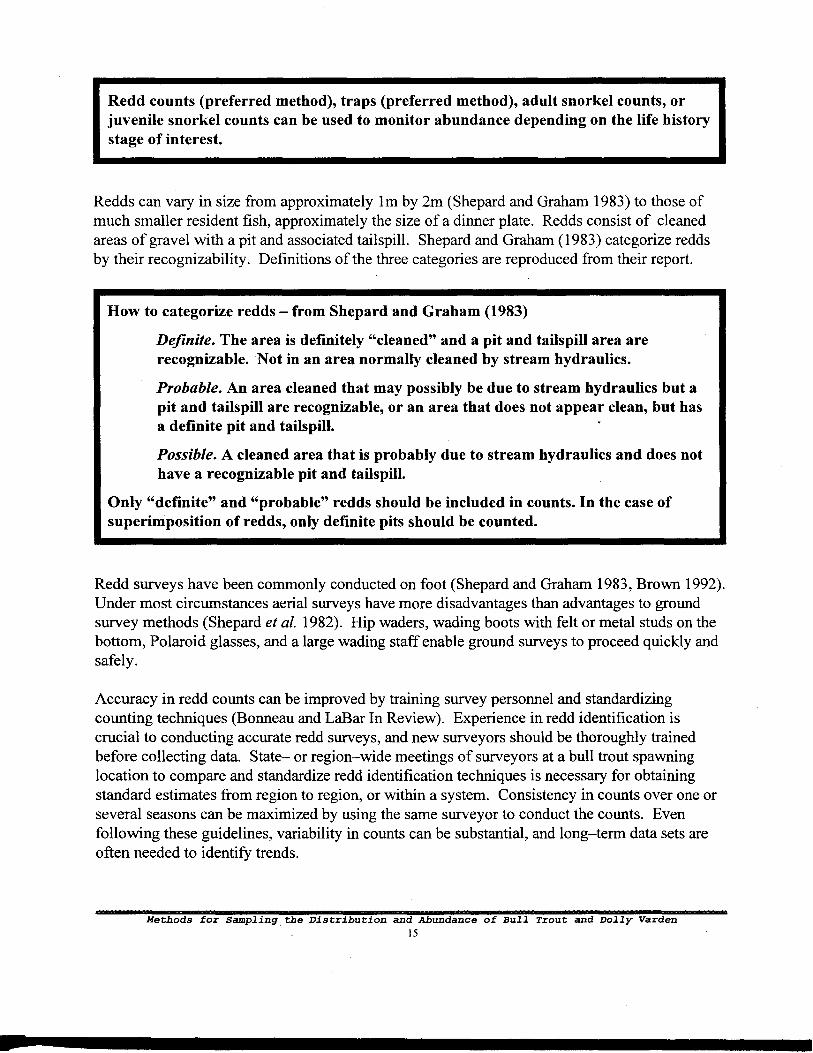
Redd counts (preferred method), traps (preferred method), adult snorkel counts, orjuvenile snorkel counts can be used to monitor abundance depending on the life historystage of interest.

Redds can vary in size from approximately 1 m by 2m (Shepard and Graham 1983) to those ofmuch smaller resident fish, approximately the size of a dinner plate. Redds consist of cleanedareas of gravel with a pit and associated tailspill. Shepard and Graham (1983) categorize reddsby their recognizability. Definitions of the three categories are reproduced from their report.

How to categorize redds — from Shepard and Graham (1983)

Definite. The area is definitely "cleaned" and a pit and tailspill area arerecognizable. Not in an area normally cleaned by stream hydraulics.

Probable. An area cleaned that may possibly be due to stream hydraulics but apit and tailspill are recognizable, or an area that does not appear clean, but hasa definite pit and tailspill.

Possible. A cleaned area that is probably due to stream hydraulics and does nothave a recognizable pit and tailspill.

Only "definite" and "probable" redds should be included in counts. In the case ofsuperimposition of redds, only definite pits should be counted.

Redd surveys have been commonly conducted on foot (Shepard and Graham 1983, Brown 1992).Under most circumstances aerial surveys have more disadvantages than advantages to groundsurvey methods (Shepard et al. 1982). Hip waders, wading boots with felt or metal studs on thebottom, Polaroid glasses, and a large wading staff enable ground surveys to proceed quickly andsafely.

Accuracy in redd counts can be improved by training survey personnel and standardizingcounting techniques (Bonneau and LaBar In Review). Experience in redd identification iscrucial to conducting accurate redd surveys, and new surveyors should be thoroughly trainedbefore collecting data. State— or region—wide meetings of surveyors at a bull trout spawninglocation to compare and standardize redd identification techniques is necessary for obtainingstandard estimates from region to region, or within a system. Consistency in counts over one orseveral seasons can be maximized by using the same surveyor to conduct the counts. Evenfollowing these guidelines, variability in counts can be substantial, and long—term data sets areoften needed to identify trends.


Cumulative numbers of redds over the entire spawning season, not individual redd counts, areneeded to calculate the total number of spawners in a system. Cumulative redd counts can beobtained by surveying each section several times during the spawning season. Surveys should bespaced close enough together in time that redds do not have a chance to appear and disappearbetween sampling periods. Currently little information is available on the length of time bulltrout redds remain visible. However, surveys are often conducted 7-14 days apart. Storms withtheir accompanying freshets can obscure redds. If conditions are favorable, some biologistssurvey immediately before storms and mark redd locations, so that the location of those reddsconstructed following the previous survey period are not lost.

Redd counts can be initiated when maximum daily water temperatures start to drop in the earlyfall. Shepard and Graham (1983) recommend conducting initial surveys when watertemperatures drop below 9°C, usually after mid to late August in Montana. In Washington, reddconstruction begins as water temperatures decline to 9-11° C (Brown 1992) and is most intenseduring September and October (Brown 1994). However, in Deep Creek, Washington, spawningstarted as early as August, and in the lowlands surrounding Puget Sound and along the coast,spawning has continued into November (Brown 1994).

The time at which spawning activity initiates can vary between individual streams. Historicalrecords on a given stream can be useful to determine spawn timing. Surveys spaced closelytogether in the early fall or late summer on streams which have not been surveyed previouslyhave been used to identify the start of spawning in eastern Washington systems (Anderson 1996).After a few years, the time at which spawning initiates can be identified with fair accuracyallowing survey times to be chosen to coincide with the spawning period. Redd surveys can beconcluded when few fish and numerous redds are found in the spawning grounds (Shepard andGraham 1983).

New redds can be marked by placing a piece of fluorescent tape tied to a tree branch near theredd with the exact location of the redd (e.g., three feet upstream, six feet toward the middle)written on it. Detailed notes can also be used to help designate redd location and redd size. Atthe end of the season, the total number of redds recorded in a notebook can be summed for anestimate of total cumulative redds. Two drawbacks of this method are that man—made debris isleft in wilderness areas and tape may be moved by anglers or hikers. If tape is left along thestream, a removal trip at the end of the year should be scheduled. When conducting surveys, caremust be taken that surveyors do not step on redds, resulting in mortality of eggs andpre—emergent fry (Kelly 1993).

For estimating abundance of chinook salmon, redds are not marked, but the total count of visibleredds over a season is divided by a visible redd life of 21 days (Smith and Castle 1994). Nostudies with which we are familiar have determined the length of visible redd life for bull trout.If resolved and not too variable, knowledge of bull trout visible redd life would aid in alleviatingthe need to mark redds.

Methods for Sampling the Distribution and Abundance of Bull Trout and Dolly ['Arden

16

To obtain cumulative redd counts:

1. Walk the spawning stream several times over the spawning season.

2. Space surveys closer together than the time it takes for redds to appear andthen disappear (approximately 7-14 days).

3. Record a new redd location by either:

a. Tying brightly—colored surveyor's tape to a nearby tree with reddlocation written on it, and/or

b. Detailed notes of new redd locations in a notebook (preferred ifpossible).

4. Sum all new redds at end of season from field notes and/or tape.

5. Remove tape during last trip at the end of the season.

Monitoring Abundance Under Conditions of Low Water Visibility and Redd Superimposition.

Often redd or snorkeling surveys are difficult to conduct because of adverse conditions.Significant bull trout spawning can occur in glacial rivers where visibility is limited. Runoffduring years with high rainfall can also lower visibility and raise water levels to make countingdifficult. Other species, such as kokanee, pink salmon, or brook trout, can spawn in the sameareas as bull trout and obliterate redds. Redd superimposition can even occur betweenovercrowded bull trout.

Almost all information describing techniques to cope with these problems is anecdotal andunpublished. Surveyors can experiment with the following methods with the understanding thattheir accuracy and precision have rarely been tested.

Glacial runoff is present in many streams in the Pacific Northwest and can limit visibilityimmensely at certain times of the year. Abundance or distribution surveys can be conductedwhen visibility is high. Surveys in glacial systems have been conducted in late fall whenfreeze—up occurs and waters clear; or in clear—water tributaries of the glacial river (Pribyl 1996,Williams 1996). It is not known whether surveys at these times or in these areas arerepresentative of the entire system. In northwestern Washington, spawning usually starts afterthe rivers clear, and glacial runoff is not generally a problem at the usual survey times (Phillips1996).

Abundance and distribution also can be ascertained using survey methods which do not dependon visibility. Thiesfeld et al. (1996) radio—tagged adults captured in Lake Billy Chinook,Oregon, and found that some were moving into a glacial—fed system to spawn. Traps,electrofishing and/or angling may be effective in systems where redd counts or snorkel surveys


are rarely practical. Sometimes no technique will be effective, and the surveyor will have toaccept annual variability in redd counts due to environmental conditions. Surveys should beconducted annually using the same technique, so relative bias due to technique used does notchange.

In the case of intra—specific superimposition of bull trout redds, Shepard and Graham (1983)recommend that only definite pits should be enumerated and included with "definite" or"probable" redd counts. Thiesfeld (1996) obtained bull trout redd counts in the presence ofspawning kokanee by decreasing the time interval between counts. Counts conducted in theMetolius River basin at intervals less than one week allowed pits and tailouts to be identifiedbefore they could be obliterated by kokanee. Kraemer (1996) tested for redd superimpositionusing rocks placed in the pit with marked with different colored ribbon for each survey. If aribbon was present for up to two weeks and then buried, redd superimposition was assumed. Ifthe ribbon was buried within a short period of time (e.g., a two—week time period), he assumedthat the redd was still under construction by the same fish, and superimposition did not occur.Sometimes, in areas where different species spawn with bull trout, surveyors might developcriteria to separate redds according to their morphometry. Redd size differs between species andsize groups within species (Wydoski and Whitney 1979).

Abundance Survey Design

Prioritizing and Selecting Sampling Sites

Clearly, all of the streams in Washington cannot be snorkeled or walked to measure bull troutabundance. Therefore, subsampling procedures are needed to monitor Washington's bull troutpopulations.

Since manpower is extremely limited for conducting surveys, streams or watersheds containingbull trout should first be prioritized for importance for monitoring. Rieman and McIntyre (1993)recommend that those systems subject to the most environmental stress should receive thehighest priority for monitoring. Bull trout populations which live in areas subjected to anglingpressure or exotic species interactions; those living in streams located close to areas undergoinglogging, development or road construction; or those living in lakes susceptible to large waterfluctuations are especially at risk. A cautionary note to using information from only impactedareas to monitor statewide trends is that a false picture of overall decline may be given. Tomonitor statewide trends, random sampling both impacted and non—impacted sites gives a morerepresentative picture. Also, sampling in areas which are not as subject to impacts givesimportant information about annual fluctuations in bull trout populations in the absence ofhuman effects.

Protection of "core areas" supporting important populations can also be used to prioritizemonitoring effort. Rieman and McIntyre (1993) discuss "core areas" and their role in


maintaining the species. They state that persistence of bull trout depends on identifying andmaintaining core areas that have the following attributes:

1) they must have all the critical habitat elements for both migratory and residentpopulations;

2) they must be selected from the best quality habitat or that which has the bestopportunity to be restored;

3) they must contain multiple subpopulations, no fewer than 5-10, so if onesubpopulation is affected by an environmental stressor, the risk can be spread, andother subpopulations can act as sources of new fish;

4) areas should be large enough to incorporate genetic and phenotypic diversity, but smallenough to ensure that the component populations effectively connect; and

5) core areas must be distributed throughout the historic range of the bull trout.

Core areas should be identified throughout the state, and those receiving the highest stress shouldreceive the highest priority for monitoring. However, as stated above, biologists should realizethat compilations of trend data from only highly disturbed sites will give an inaccurate picture ofdecline for the overall state or region

Once high—priority streams are selected for monitoring, the effort required to monitor changes inbull trout populations in those individual streams depends on the degree of precision and the typeof information required. In most cases traps or random techniques are the most accuratemeasures of changes in a watershed or stream. If very limited amount of manpower is availablefor surveys, and if knowledge of absolute escapement is not a concern, the index area techniqueis less preferable for determining changes in relative abundance over time.

Types of Survey Designs

Index Areas: Index areas have commonly been used to monitor changes in the relativeabundance of bull trout over time in a limited area, but are not accurate measures of absoluteescapement or basin—wide changes. These areas are lengths of stream or river chosen becausethey are accessible, stable, have good visibility and are representative of the spawning grounds ofa drainage (Cousens et al. 1982). Once the area is chosen, an appropriate surveying method(redd counts, adult snorkel counts or juvenile snorkel counts) is used to monitor changes in bulltrout abundance. For many of these types of surveys there is long—term data which is valuablefor monitoring trends. Additionally, these counts are convenient to conduct with limited staff.

Problems arise when extrapolating index area trends to larger regional populations. Rieman andMcIntyre (1996) found that trends in bull trout redd counts from adjacent streams or streamreaches were only weakly correlated. Therefore, trends in redd counts from an index area maynot reflect changes in adjacent sites. Index area surveys alone may miss large parts of the basin


where impacts to bull trout are occurring unless basin—wide surveys are also conducted regularly.Whenever possible, changes in abundance or estimates of total escapement for a basin or regionalpopulation should be based on trap counts of adults, counting of redds in all spawning habitat, orrandom sampling of redds. However, where index areas have been monitored for a considerableamount of time, and long—term trend data is available, researchers may want to continue thesesurveys to ensure consistency in data collection at a limited site.

Trap or Fence Counts of Adults: To obtain total estimates of escapement in a system, the trap orfence is set at the start of the tributary or stream section of interest, and the number of adultsmoving upstream are counted. This is a census of all adults migrating into that section of stream,and is useful for adfluvial, anadromous and some fluvial populations, but probably not forresidents which migrate very little (Brown 1994). Care should be taken to try to identifysubadults which migrate into areas with mature fish and introduce errors into escapementestimates. Traps should be in place during the entire spawning season, and continually checkedfor debris accumulation and vandalism that would affect trap integrity. For a detailed discussionof fence and trap design, see information compiled by Cousens et al. (1982).

Surveying an Entire Stream or Watershed: If spawning habitat is limited, it may be possible tosurvey all of the habitat in a watershed. In the North Fork Skokomish River, adfluvial bull troutspawn in only the first 2.9 km of the river above Lake Cushman and below Staircase Rapids. Allspawning habitat has been surveyed in this section of river by redd counts (Olympic NationalPark, Unpublished Data) or snorkel surveys (Collins, Unpublished Data). Since these are totalcounts, there is no associated variance.

Random Sampling of Redds Within a Watershed: Surveying all spawning habitat in awatershed several times a season is often not possible given the manpower requirements, andaircraft redd surveys are usually not effective for bull trout (Shepard et al. 1982). Expansion ofindex area redd counts rarely gives an accurate estimate of escapement in a basin, since thistechnique may miss areas where important populations are declining, especially if index areas aresmall. Therefore, subsampling of all available spawning habitat (i.e., surveying a subset ofrandomly chosen sample sections over the spawning season) may be preferable for estimates ofthe total numbers of redds and escapement where spawning areas are large and accuracy isrequired. Subsampling can be simple random (Cochran 1977), or stratified random (Cochran1977, Scheaffer et al. 1986). We propose using stratified random sampling to estimate totalabundance and escapement, since stratified random sampling requires less sampling than simplerandom techniques for an estimate of equal precision (Cochran 1977, Scheaffer et al. 1986).

Trap counts or random sampling of redds in suitable spawning habitat are appropriatefor basin—wide abundance surveys or calculating escapement.


Total redds (R) in a watershed using stratified random sampling is given by

R=Ny +Nypp nn

where Np = total number of 0.4 km sections of high-quality spawning habitat,Nn = total number of 0.4 km sections of average-quality spawning habitat,yp = average redds per 0.4 km in high-quality spawning habitat, andy„ = average redds per 0.4 km in average-quality spawning habitat.

(5)

The variance (stet') of this total is estimated by

N — n s 2 N — n s 2

s 2tot2( P= N P P) 2[ n+ N n n

1(6)

P N n n N nn

where np = number of 0.4 km sections of high-quality spawning habitat surveyed,sp2= variance of redd counts per 0.4 km in high-quality habitat,nn = number of 0.4 km sections of average-quality spawning habitat surveyed,

andsn2= variance of redd counts per 0.4 km in average-quality habitat.

We recommend bull trout spawning habitat first be divided into manageable units for footsurveys. We arbitrarily chose 0.4 km (0.25 miles) as our sampling unit for the followingexamples since it was a small distance and logistically feasible. Small sampling units givehigher precision than larger ones for simple aggregated distributions (Green 1979). Someresearchers prefer 1 or 2 km sections for logistical reasons. The following equations anddiscussion can be easily adapted for units of any size.

River sections containing the sampling units are then categorized as "high-quality" or"average-quality" spawning habitat "strata," based on the geomorphic characteristics of thereach. River habitat which is obviously not used by bull trout for spawning, such as muddylowland river sloughs, or areas where maximum water temperature does not drop below 9°C inthe fall, should not be included in the survey. Average redds per 0.4 km in each strata, and thevariance of redds per 0.4 km in each strata is calculated from randomly sampled 0.4 km surveysections in both habitat types.


To calculate the 95 percent and 80 percent confidence intervals (Cl) use the following:

R + CI =R + t\ls 2 (7)— tot

where t = 1.96 for 95 percent Cis and 1.28 for 80 percent C/s.

Example 2. Estimating the total number of redds in the North Fork Skokomish River andthe associated degree of confidence in the estimate using stratified random sampling.

A rough estimate of the length of the mainstem North Fork Skokomish River is 22.5 km. Thisconsists of 3.2 km of excellent adfluvial spawning habitat below Staircase Rapids (high—quality),and 19.3 km of sparsely populated resident spawning habitat above Staircase Rapids(average—quality). Total number of sampling units (Np and Nn) for each section is

Sampling Units (hi.qual. habitat) -

for high-quality habitat, and

Sampling Units (ave.qual.habitat) -

For average—quality habitat.

3.2 km habitat- 8

- 48

0.4 km per sampling unit

19.3 km habitat

0.4 km per sampling unit

Six randomly selected units below Staircase Rapids (nt) and eight randomly selected units (nn)above the rapids were walked over time. Cumulative average redd counts per 0.4 km in each ofthese areas were yin = 10 and y r, = 2 respectively. Variances of the redd counts were sp2 = 30 forthe high—quality habitat and sn2 = 3.43 for the average—quality habitat. Therefore, from Equation(4), an estimate of the total number of redds in the mainstem North Fork Skokomish is

R = (8)(10) + (48)(2) 176

the variance of this estimate, from Equation (5), is

S 2tot

= 82 8 - 6 30 )

8 6 482

48 - 3.43)

48 8= 903.2

and the 95 percent and 80 percent confidence intervals (C/) for the estimate, from Equation (6),are


95%C/ = 1.96 ✓903.2 = 59

and

80%CI 1.28 V903.2 = 38

respectively.

Therefore, the total number of redds in this river is estimated at 176. We are 95 percentconfident that the true number of redds is between 117 and 235, and 80 percent confident that thetrue number is between 138 and 214.

Before conducting spawning surveys, the biologist can calculate needed sample size to estimatethat the true total number of redds lies within a certain range with a desired degree of confidence.To calculate the necessary number of 0.4 km units to sample, an estimate of the standarddeviation (square root of the variance) of redds numbers in 0.4 km sections are needed, both forhigh—quality and average—quality habitat. Also a rough guess of either the mean redds per 0.4km in each strata or the total number of redds is needed to calculate a desired bound on the errorof estimation. The variance can either be obtained through a pilot survey before the actualabundance estimates start or by using the estimated range in redd counts. Tchebysheff s theorem(Scheaffer et al. 1986) and the normal distribution dictate that the range in redd counts per 0.4km (or any other survey unit length) should be roughly four to six standard deviations. Forinstance if redd counts in average—quality habitat on the Chiwawa River range from 0 to 10 reddsper 0.4 km, a rough estimate for standard deviation for less preferred habitat would be 10-0=10,then 10/4 = 2.5.

Methods for Sampling the Distribution and Abundance of Bull Trout and Dolly warden

23

Needed sample size (n) for stratified random sampling can be calculated using thefollowing:

n(No +No) 2

P P n n(7)

( CI 2+(No2 +N 02)

pp nn

Where Np= total number of 0.4 km sections in high—quality spawning habitat,N.= total number of 0.4 km sections in average—quality spawning habitat,orp = estimate of standard deviation of redds in 0.4 kin sections of high—quality

habitatan = estimate of standard deviation of redds in 0.4 km sections of

average—quality habitatCI = desired bound on the error of estimation andt = two—tailed t value associated with the desired bound on the error of

estimation (t = 1.96 for 95 percent confidence; t = 1.28 for 80 percentconfidence)

The number of total samples to allocate to each habitat type strata can be calculated usingNeyman allocation (Cochran 1977, Scheaffer et al. 1986).

Number of samples allocated to high—quality habitat (n e) is

Non = n P P

No +NoP P n n

(8)

Number of samples allocated to average—quality habitat (n.) is

nn

= n No +No

n nNo (9)

P P n n


Example 3. Determining sample size and allocation for a stratified random abundancesurvey.

An eastern Washington River, which flows from mountain headwaters to a large lake, is 43 kmlong, 32 km of which is habitat suitable for bull trout spawning. In suitable habitat there isintense spawning of bull trout in the upper 12 km, while the lower reach (20 km) supports fewspawners. This river is fed by four tributaries, two of which (Tributary A and B) are heavilyused by spawning bull trout, and two of which (Tributary C and D) support only light spawningactivity.

Total km of high-quality and average-quality habitat must first be calculated. High-qualityhabitat = 12 km in the mainstem + 2 km (length of Tributary A before an impassible waterfall) +10 km (length of tributary B). Average quality habitat = 20 km in the mainstem + 3 km (lengthof tributary C) + 14 km (length of Tributary D). Therefore, there is a total of 24 km ofhigh-quality spawning habitat and 37 km of average-quality spawning habitat in this watershed.Converting km to numbers of sampling units (Np and Nn) requires division by 0.4 km persampling unit: Np = (24)40.4)=60; Nn = (37)/(0.4)=92.

From a previous survey, redds per 0.4 km in high-quality habitat range from 1 to 5. Inaverage-quality habitat, redds per 0.4 km range between 0 to 2. Therefore estimated standarddeviation for high-quality habitat (up) is

5 - 1 = 4, and 4

4 =1.

For average-quality habitat, estimated standard deviation (an) is

2 -0 =2 and — = 0.54

Suppose the biologist wants to be 80 percent sure that the true redd count is withinapproximately + 20 percent of the estimate. Roughly he guesses from the results of a previoussurvey that an average of 2.5 redds per 0.4 km were in high-quality habitat and 0.5 redds per 0.4km were in average-quality habitat. Therefore, a rough estimate of total redds is equal to thesum of:

rough estimate of redds in high-quality habitat = (24 km of high-quality habitat /0.4 km per sampling unit) x 2.5 redds per sampling unit = 150

andrough estimate of redds in average-quality habitat = (37 km of average-qualityhabitat / 0.4 km per sampling unit) x 0.5 redds per sampling unit = 46


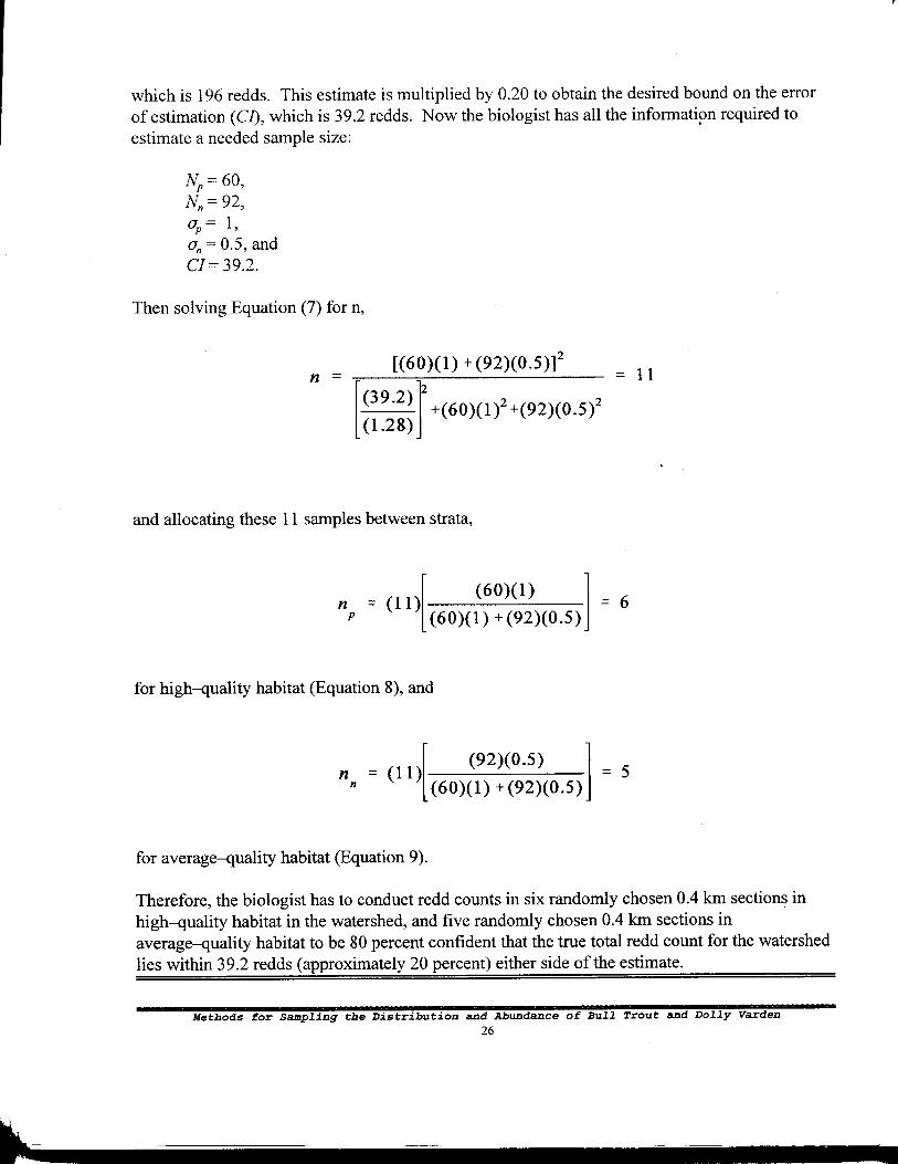
which is 196 redds. This estimate is multiplied by 0.20 to obtain the desired bound on the errorof estimation (CI), which is 39.2 redds. Now the biologist has all the information required toestimate a needed sample size:

Np = 60,Nn = 92,u

P = 1 ,

an = 0.5, andCI = 39.2.

Then solving Equation (7) for n,

n -[(60)(1) +(92)(0.5)] 2

- 11 (39.2)

(1.28)

2

+(60)(1)2 +(92)(0.5)2

and allocating these 11 samples between strata,

n = (11) (60)(1)

- 6(60)(1) + (92)(0.5)

for high-quality habitat (Equation 8), and

nn = (11) (92)(0.5) I(60)(1) + (92)(0.5)

5

for average-quality habitat (Equation 9).

Therefore, the biologist has to conduct redd counts in six randomly chosen 0.4 km sections inhigh-quality habitat in the watershed, and five randomly chosen 0.4 km sections inaverage-quality habitat to be 80 percent confident that the true total redd count for the watershedlies within 39.2 redds (approximately 20 percent) either side of the estimate.


Calculating Spawner Escapement

Estimating Escapement and Associated Confidence Intervals Using Redd Counts

Estimating Escapement: If an estimate of escapement is needed, total number of redds in thewatershed can be multiplied by spawners per redd. Ideally, number of spawners per redd isobtained by putting a trap at the mouth of the watershed, and recording the numbers of fishmigrating upstream to spawn. Simultaneously cumulative redd counts are obtained upstreamfrom the trap, and the fish count at the trap divided by the cumulative redd count gives the ratioof spawners per redd. Surveyors should exercise care when calculating these ratios. Thistechnique only works for migrating stocks (anadromous, adfluvial and some fluvial). If manybull trout in the stream of interest are residents, and do not migrate, fish to redd ratios may beunderestimated. Also, if subadults migrate into areas with mature fish, fish to redd ratios maybe overestimated.

Often fish to redd ratios are not available for a specific watershed and an estimate, derived fromother areas, is used. Because of the considerable effort involved, few spawner to redd ratios havebeen derived, and those which have been developed are widely distributed over the PacificNorthwest (Table 4). For accurate and precise estimates of escapement in Washington,

reseaxcki redd. ratios and their associated valiance for both migrating andresident populations needs to be conducted.

To calculate total escapement to a stream:

Where E = RF (10)

E = total escapement,R = total cumulative redds in a watershed or streamF = number of spawners per redd

Fish per redd can either be obtained from estimates made within the specific watershed, or anaverage of the estimates of Table 4, which is 2.2 fish per redd.


Calculating variance of escapement estimate: The variance associated with the escapementestimate is based on the total redd count and its associated variance and the spawner to redd ratioand its associated variance.

Estimate of Variance for Escapement

s 2 = s 2F 2 2 2s R

Where sE2= variance of total escapement estimate,sF = variance of fish to redd ratio,

= variance of total cumulative redd count.

Variance of total cumulative redd count, if calculated using stratified random techniques, isavailable from Equation (5). Variance in spawner to redd ratios can be obtained by monitoring atrap for several years on a stream system and calculating the variance of these estimates. Oftentrap information is unavailable from the watershed of interest, so the average spawner to reddratio from Table 4 can be substituted, and the range in these estimates can be used to calculate arough estimate of variance.

We approximated the variance in spawner to redd estimates from the range in estimates in Table4. From Tchebysheff's theorem, standard deviation (sF) of the fish to redd ratios is

1.73.2 - 1.5 = 1.7 and - 0.425

4

This quantity squared becomes the variance. Using this estimated variance of fish to redd (s,)from Table 4, Equation (11) simply becomes

S 2 = (2.2) 2sR2 + (0.425)2R 2

(12)

If the entire watershed was surveyed for redds there would be no variance associated with theredd count estimate. In each of these instances, the variance estimate would be 0, and Equation(11) would simplify to

s 2 = s 2R 2 (13)

If the variance in fish to redd ratios was estimated from Table 4 and Tchebysheff's theorem,Equation (13) becomes


28

s 2 = (0.42 2 25) R (14)

Confidence Intervals for Total Escapement Estimates: The confidence intervals for totalescapement estimates are derived from the variance of total escapement.

Confidence Intervals for total escapement estimates

E + CI E + t\ls; (15)

Where t = 1.96 for 95 percent confidence andt = 1.28 for 80 percent confidence.

Example 4. Calculating total escapement and associated confidence intervals from reddcounts.

From Example 2, the total cumulative redd count from the North Fork Skokomish river was 176with a standard deviation associated with this estimate of 30. No fish to redd estimate isavailable for this river so the average from Table 4 was used. Total escapement, from Equation(10) is

E = (176)(2.2) = 387

And variance of this estimate, from Equation (11), is

s 2 = (2.2)2 (30)2 + (0.425)2(176)2 = 9,951

80 percent confidence limits for this estimate are

387 + 80%CI = 387 + (1.28) 9,951 = 387 + 128

Therefore, we are 80 percent confident that the true total escapement lies between 259 and 515.To conservatively manage this population, we would assume that the population was 259individuals. At best it is only 515 individuals.

The next year a combination of traps and snorkeling observations conclude that there are 2.4 fishper redd in this river. No variance could be calculated from this point estimate, so the varianceestimated from the range of values in Table 4 ([0.42512) was used. As above, total escapement iscalculated using Equation (10)


E = (176)(2.4) = 422

and variance is

2SE

= (2.4)2(30)2 +(0.425)2(176)2 = 10,779


422 + (1.28)V10,779 = 133

Using the revised estimate of fish per redd, the biologist is 80 percent confident that the trueescapement in the North Fork Skokomish River is between 289 and 555.

The next year, the biologist is able to survey all bull trout spawning habitat in the North ForkSkokomish River and cumulatively counts 172 redds. The trap estimate for this river was 2.4fish per redd. There is no variance associated with the number of redds estimate, and thespawner to redd variance is estimated from the range of values in Table 4. Total escapement is

E = (172)(2.4) = 413

and variance is

S 2 = (0.425) 2(172)2 = 5,344


413 + (1.28)V5,344 = 413 + 94

Therefore, by surveying all habitat, the variance is reduced, and the biologist is 80 percentconfident that the true escapement in the North Fork Skokomish River is between 319 and 507.

Using Snorkeling Counts of Adults to Estimate Escapement

Because of fluctuating water conditions, angling and other factors, peak adult abundance countsmay not accurately reflect total spawners (Ames 1984). Measurement of the area under a curveplotted with snorkeling abundance estimates over time may provide a better representation ofspawner numbers. WDFW currently uses "area under the curve" plots of redd counts versus timeto calculate number of redd—days for other salmonids (Smith and Castle 1994). Redd—days arethen divided by the average number of days redds remain visible (21) to obtain total redds. Totalredds are then multiplied by fish to redd ratio to calculate total number of spawners. To conducta similar analysis for bull trout, with adult abundance estimates instead of redd counts, "adultdays" can be calculated. However, to convert this to total number of spawners, the averageresidence time of adults in the spawning area is needed. Since little is currently known about theresidence time of adults in spawning areas of various Washington river systems, calculation of


total spawners from adult snorkeling counts using area under the curve methods would not bereliable at this time.

Considerations When Evaluating The Status of Bull Trout Populations

Useful factors for evaluating the status of bull trout populations, such as contractions in range,rates of decline and population sizes, can be estimated using the above procedures. Smallpopulations, whether declining or not, face increased risk of extinction due to annual variationsin environmental conditions, loss of genetic variation, and demographic stochasticity (Caughleyand Gunn 1995). Therefore they may be less resilient to impacts than larger populations. Largepopulations can also have conservation problems if they exhibit a rapid rate of decline (Caughleyand Gunn 1995), and little may be done until populations have reached dangerously lownumbers.

Monitoring trends in abundance can be used to help identify bull trout populations at risk.Unfortunately, long—term data sets are often needed to determine if trends are significant (>10yrs. for redd counts, Rieman and Myers, In Press). Management actions applied only afterdeclining trends are statistically significant may be too late to prevent damage to populations.Several sources discuss how trend data can be combined with other measures of "health" toevaluate the status of bull trout populations early enough to apply appropriate managementactions(Ratliff and Howell 1992; Mongillo 1993; Rieman and McIntyre 1993; Rieman andMcIntyre 1995; Rieman and McIntyre 1996; Washington Department of Fish and Wildlife 1997;Rieman and Myers In Press). Readers can also consult conservation biology texts for generalprinciples regarding sparse or rapidly declining populations (Soule 1986; Caughley and Gunn1995).


CONCLUSIONS

(1) Distribution of bull trout can be ascertained by determining presence of bull trout in a"patch." We define a patch as a stream reach or group of reaches which includes suitablespawning and initial rearing habitat and is separated from other patches by barriers to bulltrout migration. Barriers to migration can include high water temperatures, longdistances between suitable spawning habitat, or physical barriers such as waterfalls.

(2) To determine if bull trout are present in a patch, first conduct informal surveys whichmight include angling, day or night snorkeling and/or night bank walking withinpreferred habitat in the patch. If no bull trout are found, and if a specified degree ofconfidence is wanted for lower detection limits, night snorkel 20 randomly chosen 100 msections of preferred habitat to be 95 percent confident that bull trout are in densities lessthan 0.60 fish/100 m, assuming a sampling efficiency of 25 percent. Night snorkel 11randomly chosen sections to be 80 percent confident. If other thresholds for delectabilityare required, or other sampling efficiencies are assumed, consult Appendix 2 forappropriate sample sizes. If it is not feasible to night snorkel the stream, day snorkel atwater temperatures above 9°C. If a stream is too shallow or turbid to snorkel, considerelectrofishing, at settings listed in Appendix 1 to minimize potential injury to fish.

(3) Redd surveys and traps are preferred methods for estimating total adult abundance andescapement. Redd surveys are suitable for both migrating and resident populations, whiletraps best monitor migrating fish. Obtain cumulative redd counts in a system over all thespawning habitat, or by random sampling of the habitat, depending on the accuracy andprecision desired. Multiply this estimate by 2.2 spawners per redd or preferably aspawner:redd estimate for that particular system to obtain total escapement. Continuedmonitoring of index areas can provide consistency in long—term data sets for specificareas which have been monitored for many years. However, monitoring of only indexareas is rarely appropriate for evaluating trends in an overall basin.

(4) When using redd surveys and/or traps to monitor abundance, surveyors should be awareof factors which may reduce their accuracy and precision. Bull trout can migrate forother reasons besides spawning which may inflate spawner to redd estimates derivedfrom trap counts. There is often considerable variation in the repeatability of redd counts.This can be reduced by using experienced survey crews, standardizing countingtechniques among surveyors, and whenever possible, using the same surveyors to conductcounts over a season or over several years within a system. Even following thesetechniques, long—term data sets are often needed to identify trends.

(5)

The key in Table (5) can be used to aid in selection of appropriate survey methods. Ifwater visibility is low, or redd superimposition is occurring, consider trying some of thetechniques to monitor bull trout abundance under adverse conditions which are describedin this report.


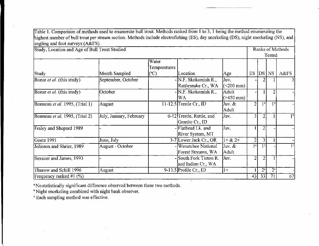
Table 1. Comparison of methods used to enumerate bull trout. Methods ranked from 1 to 3, 1 being the method enumerating thehighest number of bull trout per stream section. Methods include electrofishing (ES), day snorkeling (DS), night snorkeling (NS), andangling and foot surveys (A&FS).Study, Location and Age of Bull Trout Studied Ranks of Methods

Tested

Study Month Sampled

WaterTemperatures(°C) Location Age ES DS NS A&FS

Bonar et al. (this study) September, October - N.F. Skokomish R.,Rattlesnake Cr., WA

Juv.(<200 mm)

- 2 1 3

Bonar et al. (this study) October - N.F. Skokomish R.,WA

Adult(>450 mm)

- 1 2 -

Bonneau et al. 1995, (Trial 1) August 11-12.5 Trestle Cr.,, Juv. &Adult

2 la la -

Bonneau et al. 1995, (Trial 2) July, January, February 0-12 Trestle, Rattle, andGranite Cr., ID

Juv. 3 2 1 1b

Fraley and Shepard 1989 - - Flathead Lk. andRiver System, MT

Juv. 1 2 - -

Goetz 1991 June, July 3-7 Lower Jack Cr., OR 1+ & 2+ 2 3 1 -Johnson and Shrier, 1989 August - October - Wenatchee National

Forest Streams, WAJuv. &Adult

1 c 1 c - 1 c

Sexauer and James, 1993 - - South Fork Tieton R.and Indian Cr., WA

Juv. 2 2 1 -

Thurow and Schill 1996 August 9-13.5 Profile Cr., ID 1+ 1 2a 2a -Frequency ranked #1 (%) 43 33 71 67

a llo statistically significant difference observed between these two methods.b Night snorkeling combined with night bank observer.

Each sampling method was effective.

Table 2. Comparison of methods for determining distribution of bull trout in Washington streamsand rivers, fall 1995. Methods not tested are indicated with a "-".

Water Date(s) Day Snorkel Night SnorkelAngling andFoot Survey

Rattlesnake 9/11/95 - - 0 0Creek - 150 msection

9/13/95

Rattlesnake . 9/13/95 - 6 adults - 2 adultsCreek - 300 msection

9/13/95

Waptus River 0 - 0Basin

N.F. Skokomish 10/24/95- 0 5 juveniles 0River (Four 10/26-95Stream to UpperBridge)

N.F. Skokomish 10/28/95 79 adult bull 34 adult bull -River (Ranger trout and trout andStation to Park chinook chinooka, 3Boundary-Pools salmons, 0 juvenile bullonly) juvenile bull

trouttrout

a We did not separate adult bull trout and chinook salmon on these surveys. However, OlympicNational Park and Washington Department of Fish and Wildlife Region 6 Surveys found thatchinook salmon comprised only between 0.5 and 1.6 percent of the total run on October 19th and31st.


Table 3. Densities of juvenile bull trout encountered (e) by night snorkeling in Pacific Northweststreams and rivers.

Source River or StreamDensity (Fish/100 m ofstream)

Bonar et al. (This Report) North Fork SkokomishRiver, Washington aboveStaircase Rapids

0.26

Sexauer and James (1993) South Fork Tieton, IndianCreek, Chikamin Creek,Rock Creek, Washington

2.27-8.07

Schill (1991) Profile Creek, Idaho 5.73-42.53

Bonneau et al. (1995) Trestle Creek, Idaho 10.0-23.5


Table 4. Ratio of number of bull trout spawners to redds in various Pacific Northwest rivers.

Source LocationSpawners perRedd

Fraley and Shepard 1989 Flathead River System, MT 3.2

Ratliff et al. 1996 Jack Creek, OR (Ave. over 3 yrs.) 2.3

Ratliff et al. 1996 Jefferson Creek, OR 2.3

Pratt 1985 (cited in Brown 1994) Tributaries of Swan Lake, MT 2

James et al. Unpublished Data Indian Creek, WA 1.5

Craig and Wissmar 1993 Reach 4, Gold Creek, WA 1.8

Craig and Wissmar 1993 Reach 5, Gold Creek, WA 2.1

Average of Studies 2.2


36

Table 5. Key to help select appropriate method for sampling bull trout.

la Distribution or presence/absence information is needed 2

lb Abundance of a specific population is needed 7

2a Stream or river glacially fed, visibility usually low 3

2b Stream or river usually has good visibility 4

3a Visibility sometimes good, either in Clearwater tributaries or at various times of the yearor day 4

3b Visibility never good Go to 4 and substitute electrofishing. Alternatively set a trap atthe mouth of the system or follow radio—tagged adfluvial fish.

4a Presence/absence does not have to be defined with a specific degree ofconfidence conduct informal surveys by angling, night bank walking.and/or night andday snorkeling in preferred spawning and initial rearing habitat in a patch. We define"patch" as a stream reach or series of reaches separated from others by thermal orgeographic barriers to migration. In glacial rivers conduct surveys to coincide with timeof day or year of highest visibilities. Record the location and extent of preferred habitaton a map.

4b. Presence/absence must be defined with a specific level of confidence 5

5a. Presence/absence needs to be defined with a 95 percent or 80 percent level of confidence.Standard minimum sampling efficiency (25%) and bull trout minimum density (0.60fish/100m ) are assumed 6

5b. Presence/absence needs to be defined with a 95 percent or 80 percent level of confidence.Surveyor assumes sampling efficiency or bull trout minimum density which differs fromthat in (5a) First, do(4a), then night snorkel the number of randomly chosen 100 mstream sections in preferred habitat within a patch which corresponds with a particularminimum bull trout density, or sampling efficiency listed in Appendix 2. In areas wherenight snorkeling is not feasible, day snorkel at water temperatures > 9°C. In areas wherewater is too shallow for snorkeling and conductivity is adequate (approaching 100µS/cm), electrofish using guidelines in Appendix 1.

6a. Presence/absence needs to be defined with a 95 percent level of confidence First, do(4a), then night snorkel 20 randomly chosen 100 m stream sections in preferred habitatwithin a patch to determine bull trout are in densities less than 0.60 fish/100 m, assuminga minimum sampling efficiency of 25 percent. In areas where night snorkeling is not


feasible, day snorkel at water temperatures > 9°C. In areas where water is too shallow forsnorkeling and conductivity is adequate (approaching 100 µS/cm), electrofish usingguidelines in Appendix 1.

6b. Presence/absence needs to be defined with a 80 percent level of confidence First, do(4a), then night snorkel 11 randomly chosen 100 m stream sections in preferred habitatwithin a patch to determine bull trout are in densities less than 0.60 fish/100 m, assuminga minimum sampling efficiency of 25 percent. In areas where night snorkeling is notfeasible, day snorkel at water temperatures > 9°C. In areas where water is too shallow forsnorkeling and conductivity is adequate (approaching 100 0/cm), electrofish usingguidelines in Appendix 1.

7a. An estimate of absolute escapement from a watershed or river system is needed 8

7b. An estimate of absolute escapement is not needed monitor abundance using cumulativeredd counts (preferred), traps (preferred), adult snorkel counts, or juvenile snorkel countsdepending on the life history stage of interest. Abundance can be monitored in indexareas (less preferred except where historical trend data exists and accurate only for trendsin the index area sampled); by surveys of the entire system; or by using stratified randomtechniques. If abundance estimates are needed in a glacial low—visibility system, conductsnorkel surveys or redd counts during periods of higher visibility such as late fall or inclear water tributaries. If kokanee are spawning in the same area, decrease the timeinterval between redd counts so kokanee have less time to obliterate evidence of bull troutredds. Other methods listed in this report may also be effective for conducting reddcounts under conditions of superimposition.

8a. Absolute escapement is needed for migrating (fluvial, adfluvial, anadromous)populations monitor abundance using cumulative redd counts or traps. If using reddcounts, either survey the entire spawning area or sample sections of it using the stratifiedrandom techniques described in this report. If kokanee are spawning in the same area,decrease the time interval between redd counts so kokanee have less time to obliterateevidence of bull trout redds. Other methods listed in this report may also be effective forconducting redd counts under conditions of superimposition.

8b. Absolute escapement is needed in a river or stream which contains both migrating andresident populations monitor abundance using cumulative redd counts. If using reddcounts, either survey the entire spawning area or sample sections of it using the stratifiedrandom techniques described in this report. If kokanee are spawning in the same area,decrease the time interval between redd counts so kokanee have less time to obliterateevidence of bull trout redds. Other methods listed in this report may also be effective forconducting redd counts under conditions of superimposition.


REFERENCES

Ames, J. 1984. Puget sound chum salmon escapement estimates using spawner curvemethodology. Pages 133-148 in P.E.K. Symons and M. Waldichuk, editors. Proceedingsof the Workshop on Stream Indexing for Salmon Escapement Estimation, WestVancouver, B.C., 2-3 February 1984. Canadian Technical Report Fisheries and AquaticSciences No. 1326: xv + 258 pp.

Anderson, E . 1996 . [Personal communication\ . Y akima \Wk. W ashington Department of F ishand Wildlife.

Anonymous 1995a. 1995-1996. Fishing in Washington. Sport Fishing Rules, Pamphlet Edition.Washington Department of Fish and Wildlife. 120 pp.

Anonymous 1995b. Bull trout/dolly Varden management plan. Draft programmaticenvironmental impact statement. Washington Department of Fish and Wildlife TechnicalReport. 61 pp.

Anonymous 1996. Inland fish investigations in Washington. 1994 Annual Progress Report.Washington Department of Fish and Wildlife Technical Report. 356 pp.

Bonneau, J.L. 1995. [Personal communication]. Boise ID: University of Idaho Department ofFish and Wildlife Resources.

Bonneau, J.L., R.F. Thurow, D.L. Scarnecchia. 1995. Capture, marking, and enumeration ofjuvenile bull trout and cutthroat trout in small, low—conductivity streams. NorthAmerican Journal of Fisheries Management 15:563-568.

Bonneau, J.L. and G. LaBar. In Review. Inter—observer and temporal variability in bull trout reddcounts in tributaries of Lake Pend Oreille, Idaho. North American Journal of FisheriesManagement.

Brown, L.G. 1992. Draft management guide for the bull trout Salvelinus confluentus (Suckley)on the Wenatchee National Forest. Washington Department of Wildlife Technical Report.104 pp.

Brown, L.G. 1994. On the zoogeography and life history of Washington's native char.Washington Department of Fish and Wildlife Technical Report 94-04.

Buckman, R.C., W.E. Hosford, and P.A. Dupee. 1992. Malheur River bull trout investigations.Pages 45-57 in P.J. Howell and D.V. Buchanan, editors. Proceedings of the GearhartMountain bull trout workshop. American Fisheries Society, Oregon Chapter, Corvallis.


Caughley, G., and A. Gunn. 1995. Conservation biology in theory and practice. BlackwellScience, Cambridge, Massachusetts.

Cochran, W.G. 1977. Sampling Techniques, 3rd Edition. John Wiley and Sons, New York. 428

PP.

Collins, D. Unpublished data. Montesano WA: Washington Department of Fish and Wildlife.

Cousens, N.B.F., G.A. Thomas, C.G. Swann, and M.C. Healey. 1982. A review of salmonescapement estimation techniques. Canadian Technical Report of Fisheries and AquaticSciences No. 1108. 122 pp.

Craig, S.D., and R.C. Wissmar. 1993. Habitat conditions influencing a remnant bull troutspawning population, Gold Creek, Washington. Draft Report. Fisheries ResearchInstitute, University of Washington.

Cummins, J. 1995 [Personal communication]. Yakima WA: Washington Department of Fish andWildlife.

Dambacher, J.M., M.W. Buktenica and G.L. Larson. 1992. Distribution, abundance, and habitatutilization of bull trout and brook trout in Sun Creek, Crater Lake National Park, Oregon.Pages 30-36 in P.J. Howell and D.V. Buchanan, editors. Proceedings of the GearhartMountain bull trout workshop. American Fisheries Society, Oregon Chapter, Corvallis.

Dwyer, W.P., and D.A. Erdahl. 1995. Effects of electroshock voltage, wave form, and pulse rateon survival of cutthroat trout eggs. North American Journal of Fisheries Management15:647-650.

Faler, M.P. 1995. An evaluation using a mark—recapture population estimator as a monitoringtool for an adfluvial bull trout population. Aqua—Talk. R-6 Fish Habitat RelationshipTechnical Bulletin #9. USDS Forest Service, Carson, WA.

Fraley, J.J., and B.B. Shepard. 1989. Life history, ecology and population status of migratorybull trout (Salvelinus confluentus) in the Flathead Lake and River System, Montana.Northwest Science 63:133-143.

Fraley, J., T. Weaver, and J. Vashro. 1989. Cumulative effects of human activities on bull trout(Salvelinus confluentus) in the Upper Flathead Drainage, Montana. In HeadwatersHydrology, American Water Resources Association.

Fredenberg, W. 1992. Evaluation of electrofishing—induced spinal injuries resulting from fieldelectrofishing surveys in Montana. Montana Department of Fish, Wildlife and ParksTechnical Report.


Goetz, F. 1991. Bull trout life history and habitat study. Oregon State University TechnicalReport.

Green, R.H. 1979. Sampling design and statistical methods for environmental biologists. JohnWiley and Sons, New York.

Green, R.H. and R.C. Young. 1993. Sampling to detect rare species. Ecological Applications3:351-356.

Harkenrider, D.T. District Ranger, Mt Baker—Snoqualmie National Forest, Skykomish, WA.Letter dated May 17, 1994 to bull trout workshop participants outlining surveymethodology in the Mt. Baker—Snoqualmie National Forest.

Hillman, T.W., and W.S. Platts. 1993. Survey plan to detect the presence of bull trout. DonChapman Consultants Incorporated, Boise, ID. Technical Report.

James, P., J. Cummins and E. Anderson. Unpublished bull trout data from Indian Creek. CentralWashington University and Washington Department of Fish and Wildlife

Johnson, T.H. and F. Shrier. 1989. Bull trout studies in Washington. Washington Department ofWildlife Technical Report 93-21.

Kelly, B.K. 1993. Ecology of yellowstone cutthroat trout and an evaluation of potential effects ofangler wading in the Yellowstone River. Master's Thesis. Montana State University.Bozeman.

Kelly, B.K. 1997. Analysis of fish populations in Icicle, Trout, Jack, Peshastin, Ingalls, andNegro creeks, Washington. U.S. Fish and Wildlife Service, Leavenworth.

Kraemer, C. 1996 [Personal communication]. Mill Creek WA: Washington Department of Fishand Wildlife.

McPhail, J.D., and J.S. Baxter. 1996. A review of bull trout (Salvelinus confluentus) life—historyand habitat use in relation to compensation and improvement opportunities. BritishColumbia Ministry of Environment, Lands and Parks Fisheries Management Report No.104.

McPhail, J.D., and C. Murray. 1979. The early life history and ecology of Dolly Varden(Salvelinus malma) in the upper Arrow Lakes. Report to the B.C. Hydro and PowerAuthority and Kootenay Department of Fish and Wildlife.

Mongillo, P. 1993. The distribution and status of bull trout/Dolly Varden in Washington state.Washington Department of Fish and Wildlife Technical Report 93-22. 45 pp.


Mullan, J.W., K. Williams, G. Rhodus, T. Hillman, and J. McIntyre. 1992. Production andhabitat of salmonids in mid—Columbia River tributary streams. U.S. Fish and WildlifeService Monograph 1.

Olympic National Park. Unpublished Data. Hoodsport WA.

Pratt, K., 1985. Pend Oreille trout and char life history study. Idaho Department of Fish andGame.

Phillips, C. 1996 [Personal communication] Mill Creek WA: Washington Department of Fishand Wildlife.

Pribyl, S. 1996 [Personal communication] The Dalles OR: Oregon Department of Fish andWildlife.

Ratliff, D.E., and P.J. Howell. 1992. The status of bull trout populations in Oregon. Pages 10-17in P.J. Howell and D.V. Buchanan, editors. Proceedings of the Gearhart Mountain bulltrout workshop. American Fisheries Society, Oregon Chapter, Corvallis.

Ratliff, D.E., S.L. Thiesfeld, W.G. Weber, A.M. Stuart, M.D. Riehle and D.V. Buchanan. 1996.Distribution, life history, abundance, harvest, habitat, and limiting factors of bull trout inthe Metolius River and Lake Billy Chinook, Oregon. 1983-1994. Oregon Department ofFish and Wildlife Technical Report.

Rieman, B.E. 1997. [Personal Communication] Boise, ID: U.S. Forest Service.

Rieman, B.E., and J.D. McIntyre. 1993. Demographic and habitat requirements for conservationof bull trout. U.S. Forest Service Intermountain Research Station General TechnicalReport INT-302.

Rieman, B.E., and J.D. McIntyre. 1995. Occurrence of bull trout in naturally fragmented habitatpatches of varied size. Transactions of the American Fisheries Society 124:285-296.

Rieman, B.E., and J.D. McIntyre. 1996 Spatial and temporal variability in bull trout redd counts.North American Journal of Fisheries Management 16:132-141.

Rieman, B.E., and D.L. Myers. In Press. Use of redd counts to detect trends in bull troutpopulations. Conservation Biology.

Scheaffer, R.L., W. Mendenhall, and L. Ott. 1986. Elementary survey sampling, 3rd edition.PWS-Kent, Boston. 324 pp.


Schill, D.J. 1991. River and stream investigations: Bull trout aging and enumerationcomparisons. Idaho Fish and Game Job Performance Report, Project F-73—R-13.

Schreck, C.B., R.A. Whaley, M.L. Bass, O.E. Maughan, and M. Sola77i 1976. Physiologicalresponses of rainbow trout (Salmo gairdneri) to electroshock. Journal of the FisheriesResearch Board of Canada 33:76-84.

Sexauer, H.M., and P.W. James. 1993. A survey of the habitat use by juvenile and pre—spawningadult bull trout, Salvelinus confluentus, in four streams in the Wenatchee national forest.Central Washington University, Department of Biological Sciences Technical Report.

Sharber, N.G., and S.W. Carothers. 1988. Influence of electrofishing pulse shape on spinalinjuries in adult rainbow trout. North American Journal of Fisheries Management 8:117-122.

Shepard, B., T. Weaver, J. Fraley and P. Graham. 1982. Flathead River fishery study. MontanaDepartment of Fish, Wildlife and Parks, Kalispell, MT.

Shepard, B.B., and P.J. Graham. 1983. Fish resource monitoring program for the upper flatheadbasin. Flathead River Basin Environmental Study, EPA Contract No. R008224-01-4.

Smith, C.J. and P. Castle. 1994. Puget Sound chinook salmon (Oncorhynchus tshawytscha)escapement estimates and methods - 1991. Washington Department of Fish and Wildlife,Northwest Fishery Resource Bulletin Project, Report Series Number 1.

Soule, M.E.. 1986. Conservation biology: the science of scarcity and diversity. Sinauer,Sunderland, Massachusetts.

Thiesfeld, S. L. 1996. [Personal communication]. Prineville OR: Oregon Department of Fish andWildlife.

Thiesfeld, S.L., A.M. Stuart, D.E. Ratliff, and B.D. Lampman. 1996. Migration patterns of adultbull trout in the Metolius River and Lake Billy Chinook, Oregon. Oregon Department ofFish and Wildlife Information Report 96-1.

Thurow, R.F. 1994. Underwater methods for study of salmonids in the intermountain west.General Technical Report INT—GTR-307. Ogden, UT: U.S. Department of Agriculture,Forest Service, Intermountain Research Station.

Thurow, R.F. 1997. Habitat utilization and diel behaviour of juvenile bull trout (Salvelinusconfluentus) at the onset of winter. Ecology of Freshwater Fish 6:1-7.

Methods for Sampling the Distribution and Abundance of Bull Trout and Dolly warden43

Thurow, R.F. and D.J. Schill. 1996. Comparison of day snorkeling, night snorkeling, andelectrofishing to estimate bull trout abundance and size structure in a second—order Idahostream. North American Journal of Fisheries Management 16:314-323.

Washington Department of Fish and Wildlife. 1996. Draft Washington state salmonid stockinventory: Bull trout/Dolly Varden.

Weaver, T. and J. Fraley. 1991. Fisheries habitat and fish populations. Flathead basin forestpractice water quality and fisheries cooperative program. Flathead Basin Commission,Kalispell, MT. 47 pp.

Williams, K. 1996. [Personal communication] Ephrata WA: Washington Department of Fish andWildlife.

Wydoski, R.S., and R.R. Whitney. 1979. Inland fishes of Washington. University of WashingtonPress, Seattle.


Appendix 1. Stream electrofishing guidelines for Washington Department of Fish and Wildlifedistribution (stream typing) surveys.


45

ELECTROFISHING GUIDELINES FOR STREAM TYPING

Primary Goal: In order to correctly prove presence/absence of salmonids in streams presumed to be fish bearing,electrofishing techniques must provide the highest probability possible for detecting salmonid presence.

Secondary Goal: Within the range of effective electrofishing techniques, sampling should be conducted to minimize injuryto fish and other aquatic and terrestrial animals.

Environmental/Biological Factors:5) No electrofishing should be conducted when temperatures are below 4° C or above 24° C.6) No electrofishing should be conducted when samplers cannot clearly see the stream bottom in one foot of

water.7) Once a fish is found, discontinue shocking. Move upstream until habitat parameters change, which might

indicate a change in the status of fish presence, and resume shocking.8) Remove netted fish from electrical field immediately; do not hold fish in net while continuing to net additional

fish.

Equipment Factors:1) Use electrofishing units with straight direct current (DC) settings if at all possible.2) If straight DC is not an option, begin by sampling with lower frequencies or pulse rates (i.e. 30 Hz).3) Avoid electrofishing units that cannot produce pulsed DC with frequencies less than 60 Hz.4) If pulse width is a programmable option on your unit, use 5 milliseconds, which has proven to be highly

effective under a wide range of conductivities and minimizes injury rates.5) Never use any form of alternating current (AC) output.

Testing and Programming Equipment:In order to increase electrofishing efficiency, equipment needs to be tested and programmed correctly for the specificdrainage. The intent is that if the sampler can first be successful in netting fish within known fish-bearing segments, he/shewill have a higher confidence and probability of finding fish within segments where presence is uncertain. Use the proceduredescribed below before beginning your official stream typing.

A. Go downstream from the segment in which the stream typing is to be conducted to a known fish-bearing areawith a high probability of finding fish. Areas below culverts, deeper pools with woody cover, etc. are good placesto start. This testing should be conducted on the same day as the stream typing in order to avoid environmentalchanges which may affect electrofishing efficiency.

B. With the recommended straight DC, start with lower voltages (i.e. 200 V). If fish are not drawn close enough toanode to be netted (after 5 minutes of shocking) at lower voltage setting, increase to next higher voltage setting (upto a maximum of 800 V). Low to moderate voltage settings (300-500 V) are most commonly used. As soon as fishcan be drawn close enough to anode to be netted, use those settings for stream typing. If fish cannot be drawn toanode, proceed to "C". [Remember: Keep power switch on until fish is netted; otherwise, fish will dart away.]

C. With pulsed DC, start with lower frequency and voltage (30 Hz and 300 Volts). If fish are not drawn close enoughto anode to be netted (after 5 minutes of shocking) at lower voltage setting, increase to next higher voltage setting(keeping frequency the same).

D. If lower frequency setting (30 Hz) is ineffective in drawing fish close enough to anode to be netted, even at highervoltage settings, then turn frequency up to next setting (40 Hz) and repeat as in step "C". Follow the same steps for50 Hz and 60 Hz if necessary. Sixty (60) Hz should be the highest frequency necessary. Due to higher injury rates,60 Hz should be used as last resort. [Remember: Increase voltage settings before going to higher frequencysetting.]

Scientific Collector's Permit Attachment for Stream Typing (3/6/97)

46

Appendix 2. Encounter densities (e) and number of 100m stream sections (n) to be surveyed for detecting bull trout with 95 percentconfidence at a variety of sampling efficiencies and mean densities. For example, three 100 m sections of stream need to be sampled todetect bull trout if they are in densities of 1.5 fish/100m with 95 percent confidence, assuming the gear type used has a samplingefficiency of 75 percent. The number of fish which will be encountered using the gear type is e = 1.125 fish/100 m.

Sampling Efficiency (%)

100 90 80 75 50 25 10

Mean Density(fish/100 m)

e n e n e n e n e n e n e n

5.000 5.000 1 4.500 1 4.000 1 3.750 1 2.500 2 1.250 3 0.500 6

4.000 4.000 1 3.600 1 3.200 1 3.000 1 2.000 2 1.000 3 0.400 8

3.000 3.000 1 2.700 2 2.400 2 2.250 2 1.500 2 0.750 4 0.300 10

2.000 2.000 2 1.800 2 1.600 2 1.500 2 1.000 3 0.500 6 0.200 15

1.500 1.500 2 1.350 3 1.200 3 1.125 3 0.750 4 0.375 8 0.150 20

1.000 1.000 3 0.900 4 0.800 4 0.750 4 0.500 6 0.250 12 0.100 30

0.750 0.750 4 0.675 5 0.600 5 0.563 6 0.375 8 0.188 16 0.075 40

0.60 0.600 5 0.540 6 0.480 7 0.450 7 0.300 10 0.150 20 0.060 50

0.500 0.500 6 0.450 7 0.400 8 0.375 8 0.250 12 0.125 24 0.050 60

0.250 0.250 12 0.225 14 0.200 15 0.188 16 0.125 24 0.063 48 0.025 120

0.100 0.100 30 0.090 34 0.080 38 0.075 - 40 0.050 60 0.025 120 0.010 300

Appendix 2. Continued. Encounter densities (e) and number of 100m stream sections (n) to be surveyed for detecting bull trout with 80percent confidence at a variety of sampling efficiencies and mean densities.

Sampling Efficiency (%)

100 90 80 75 50 25 10

Mean Density(fish/100 m)

e n e n e n e n e n E n e n

5.000 5.000 1 4.500 1 4.000 1 3.750 1 2.500 1 1.250 2 0.500 4

4.000 4.000 1 3.600 1 3.200 1 3.000 1 2.000 1 1.000 2 0.400 4

3.000 3.000 1 2.700 1 2.400 1 2.250 1 1.500 2 0.750 3 0.300 6

2.000 2.000 1 1.800 1 1.600 1 1.500 2 1.000 2 0.500 4 0.200 8

1.500 1.500 2 1.350 2 1.200 2 1.125 2 0.750 3 0.375 5 0.150 11

1.000 1.000 2 0.900 2 0.800 2 0.750 3 0.500 4 0.250 7 0.100 16

0.750 0.750 3 0.675 3 0.600 3 0.563 3 0.375 5 0.188 9 0.075 22

0.60 0.600 3 0.540 3 0.480 4 0.450 4 0.300 6 0.150 11 0.060 27

0.500 0.500 4 0.450 4 0.400 4 0.375 5 0.250 7 0.125 13 0.050 32

0.250 0.250 7 0.225 8 0.200 8 0.188 9 0.125 13 0.063 26 0.025 64

0.100 0.100 16 0.090 18 0.080 20 0.075 22 0.050 32 0.025 64 0.010 160

Whntn - Yakima Basin Fish and Wildlife Recovery Board · Whntn prtnt f IS nd WIIE thd fr pln th...

Documents

Transcript of Whntn - Yakima Basin Fish and Wildlife Recovery Board · Whntn prtnt f IS nd WIIE thd fr pln th...