When Distance Shrinks: The Effects of Competitor

Proximity on Firm Survival

Jasmina Chauvin∗

JOB MARKET PAPER

[Manuscript in Progress. Please Do Not Distribute or Cite]

October 31, 2017

AbstractWhat are the performance implications of co-locating with firms in one’s

industry? The existing empirical evidence is mixed. In this paper, I arguethat proximity between firms affects their performance differently depending onwhether they compete locally or in broader national markets. I capture changesin co-location using a new approach, where road infrastructure investments pro-vide exogenous variation in the proximity between firms. Combining detaileddata on the location of all manufacturing firms with changes in minimum traveltimes between them in the context of Brazil, I find that in locally traded in-dustries greater proximity breeds competition. It leads to exit of the smallestfirms and improved survival prospects of the largest. As proximity increases,firms react strategically, by switching products and relocating to lower expo-sure to competitors. The effects differ in nationally traded industries. Hereproximity increases the survival rate and results in fewer relocations, consistentwith increased agglomeration spillovers. The results shed light on contradictoryfindings in the literature and show how changes in the actual costs of mobilityintensify both competition and agglomeration forces.

∗Harvard Business School. jchauvin@hbs.edu. I am grateful to Juan Alcácer, Laura Alfaro, andWilliam Kerr for invaluable guidance and support. This project has benefitted from discussionswith Pol Antràs, Carlos Azzoni, Joel Baum, Kirill Borusyak, Michele Coscia, Claudio Ferraz, JeffryFrieden, Tarun Khanna, Hong Luo, Brian McCann, Marc Melitz, Frank Neffke, John Van Reenen,Olav Sorenson, Claudia Steinwender, Chad Syverson, Eric Werker, Richard Zeckhauser, and par-ticipants at the HBS Strategy Student Seminar and the 2017 BPS Dissertation Workshop. Specialthanks to Newton de Castro and Eduardo Haddad for sharing the Brazilian transportation data andto the Harvard Center for Geographic Analysis for technical support. This project received fundingfrom Harvard Business School and the David Rockefeller Center for Latin American Studies.

1

1 Introduction

Geographic proximity between firms in the same industry, co-location, is a double-edged sword. In theory it can give rise to positive agglomeration economies – benefitsthat stem from denser local pools of workers, inputs, ideas, or demand (Marshall1920). But co-location can also breed competition over local customers (Hotelling1929) and resources (Hannan and Freeman 1977). The empirical literature asking howco-location of firms in the same industry affects performance has arrived at positive,negative, and null results depending on the set of industries and firms analyzed (e.g.Baum and Mezias 1992, Sorenson and Audia 2000, Henderson 2003, Acs et al., 2007,Buenstorf and Klepper 2009). This state of the literature, which has been called“tentative” (McCann and Folta 2008) and “troublesome”, (Arikan and Schilling 2011)might not be entirely surprising in light of theory. It points to the possibility thatthe net effect of agglomeration benefits and competition forces differs across firmsand industries. The question, then, is: which firms benefit and which are hurt byproximity to competitors?

In this paper I provide causal evidence of a key dimension of heterogeneity thatdetermines how co-location affects firm performance: the geographic scope of compe-tition. Combining insights from models of spatial competition and of agglomeration(Hotelling 1929, Syverson 2004, Combes et al. 2012), I argue that in industries wherefirms compete locally (e.g. concrete, dairy), the competition effects dominate andincreased proximity between firms leads to a process of competition-driven selection,i.e. a “weeding out” of the least productive firms from the market. Meanwhile innationally traded industries (e.g. car parts, electronics), the agglomeration benefitsdominate and increased proximity improves the survival prospects of co-located firms.

To identify the effects of co-locating with competitors on firm performance I in-troduce a new empirical approach, which uses road upgrades as an exogenous shockto co-location. It addresses problems associated with endogenous firm location choiceand unobserved heterogeneity that plague existing measures based on firm entry, exit,and growth dynamics. It also echoes recent findings that actual costs of mobility andcommunication like those shaped by the road network, rather than distance per se,define cluster shapes (Kerr and Kominers 2015) and the spatial scope of competition(Haveman and Rider 2014).

The setting is Brazil, where the federal government invested more than 70 billion

2

reals (roughly US$ 35 billion) during 2007-2014 in road upgrades under the Programade Aceleração do Crescimento (“PAC”). Building on methods from the burgeoningliterature in spatial economics, I collect detailed geospatial data on the road networkand its condition before and after the program to calculate how it affected travel timesbetween all Brazilian municipalities (geographic units slightly smaller than U.S. coun-ties). I combine the travel times with exhaustive data on the location and operationsof all formal sector manufacturing firms to measure how co-location changed onlydue to changes in minimum travel times stemming from road upgrades. In order toavoid well-known problems in using arbitrary administrative boundaries, I define eachfirm’s local market organically, as the geographic area that it can reach within fourhours (a one day’s drive including return trip).

An important concern is that road upgrades may be targeted to particular lo-cations that are expected to perform well in the future. My identification strategyaddresses this possibility by including a rich set of fixed effects for each Brazilian mu-nicipality and each industry. Thus, identification exploits only the variation acrossindustries in the same municipality, which stem from differences in industries’ pre-existing location patterns. This can be illustrated with a simple example. Considertwo firms, one producing ice cream and the other soft drinks in the Brazilian mu-nicipality of Uberlandia. Assume that in 2007, other ice cream producers in thevicinity of Uberlandia happened to lie mostly to the west while other local soft drinksmanufacturers were located mostly to the east of Uberlandia. If Uberlandia saw anupgrade on a road leading westward, the ice cream producer would see a larger shockto co-location than the soft drink manufacturer. Unless the government programsystematically sought to connect firms in specific industry-municipality pairs in themanufacturing sector to one another,1 this strategy will yield causal identification ofthe effects of co-location on performance.

Studying the effects of changes in co-location on manufacturing firms’ survivalrates, I find strong support for the prediction of heterogeneous effects in locally andnationally traded industries. Using the Ellison-Glaser (1997) index to identify whichindustries geographically spread out (locally traded) versus concentrate (nationally

1Conversations with the government secretariat in charge of the PAC road investment programsuggest that while economic considerations entered investment decisions, those tended to be sensitiveto the needs of largest exporting sectors (e.g. soy and corn) rather than manufacturing. Projectchoice was also constrained by the existence of feasibility studies and capacity constraints on theexisting network.

3

traded), I find that in locally traded industries, doubling co-location reduces thesurvival probability of the smallest firms by 14.1 percentage points and increases thesurvival rate of the largest firms by 2.6 percentage points (given an average survivalprobability of 46.2 and 64.1 percent, respectively). This firm-level heterogeneity isin line with the prediction of competition-driven selection, i.e. the weeding out ofthe smallest firms from the market, and reallocation of market power to the largestfirms. In contrast, in nationally traded industries doubling co-location increases firms’survival probability by 14.9 percentage points (given an average survival probabilityof 55.4 percent), with no significant differences across firm sizes.

Additional analyses that study firms’ strategic responses to the road shocks, specif-ically the prevalence of product-switches and relocations, find further evidence consis-tent with the heterogeneous effects hypotheses. I find that when co-location increases,firms in locally traded industries become more likely to switch their primary productor relocate to a different municipality. Firms that switch or relocate, tend to do soin a way that lowers co-location relative to their original choice of industry and loca-tion, a finding suggestive of competitive repositioning (Gimeno, Chen, and Bae 2006,Shaver and Wang 2014). Meanwhile in nationally traded industries, when co-locationincreases, firms become less likely to relocate. When they relocate or switch theirprimary product, they tend to increase co-location by moving toward firms in theirindustry, a finding that is consistent with resource-seeking agglomeration (Chung andAlcácer 2002, Kalnins and Chung 2004).

I consider a number of alternative explanations and find that these results are notdriven by increased local market access, competition from new entrants, increasedproximity to export markets, importing and exporting firms, or pre-period trends.I also do not find evidence of surviving companies getting bigger, e.g. due to con-solidation or effects on the labor market via higher wages. While I cannot test themechanisms directly (without observing local prices, knowledge flows, etc.), the re-sults are consistent with proximity increasing competition in locally traded industriesand facilitating agglomeration spillovers in nationally traded industries.

This paper contributes to the empirical literature on the performance effects of co-location. It identifies a key dimension of heterogeneity in the proximity-performancerelationship across industries which can help to explain why studies that focus onsingle industries may arrive at positive (e.g. Chung and Kalnins 2001, Henderson2003), negative (e.g. Baum and Mezias 1992, Sorenson and Audia 2000, Folta et al.

4

2006), mixed (Beaudry and Swann 2009), and null results (Buenstorf and Klepper2009) while those that estimate average effects across manufacturing may find small(e.g. Martin, Mayer, and Mayneris 2011) or null effects (e.g. Basile, Pittiglio, andReganati 2017) depending on the composition of firms and industries in the sample.Beyond industry-level heterogeneity, I also find differences in the effects of co-locationfor small and large firms (Shaver and Flyer 2000, Alcácer 2006, McCann and Folta2011). Methodologically, I introduce a new empirical approach, leveraging changesto the costs of mobility to arrive at alternative, more exogenous, measures of changesin co-location.

This paper also contributes to an active empirical literature on the effects of trans-portation infrastructure investments. While governments around the world spendbillions of dollars annually on transportation infrastructure, until recently, causalevidence regarding the impact of such investments was lacking. New advances indigital mapping and geo-spatial data analysis have given rise to a flurry of researchin this area. There is strong evidence that infrastructure investments affect welfare(Donaldson 2010), regional growth dynamics (Faber 2014; Ghani, Goswami, Kerr,2015), innovation (Agrawal et al. 2016), and entry (Gibbons et al., 2017). This paperhighlights the effect of such investments on competition and agglomeration spillovers,revealing important heterogeneity in how firms are affected by increased proximity toother firms in their industry.

Finally, this paper contributes to a related stream of research in the internationaleconomics literatures that seeks to disentangle the positive spillover and negativecompetition effects on local firms from the entry of FDI (Aitken and Harrison 1999;Alfaro and Chen 2017) and of increased import competition on firm performance (e.g.Bloom et al. 2016, Chen and Steinwender 2016). The contribution of the currentpaper is to show that similar dynamics that arise following decreases in the costsof cross-border interactions also take place when “distances shrink” within nationalboundaries.

2 Conceptual Framework

The key argument I put forth in this section is that the effect of increased co-locationwill differ for firms in industries that compete locally and those that compete na-tionally. First, I summarize the state of the literature which motivates an inquiry

5

into industry-level differences. I then discuss conceptually the nature of locally andnationally traded industries and sketch a framework to highlight the source of hetero-geneous effects. The framework informs the hypotheses tested in the empirical partof the paper.

2.1 Co-location, Competition, Agglomeration

Strategy research acknowledged the duality of proximity as a force of both compe-tition and agglomeration early on and has asked how these dual forces shapes firmlocation strategy. In one of the earliest studies to do so, Baum and Haveman (1997)show that product and geographic location choices of newly founded hotels in Man-hattan appear to balance agglomeration (co-locating with similarly priced hotels)with differentiation (on size). Subsequent studies show further heterogeneity in howfirms trade off agglomeration benefits and competition in their location choices. Forexample Shaver and Flyer (2000) show that small firms co-locate (seek agglomera-tion benefits) while large firms no not (avoid competition). Alcácer (2006) showsthat firms co-locate versus disperse depending on the value-chain function, seekingspillovers in R&D activities but avoiding competition in sales.

While the literature on location choice illustrates strong patterns of co-location(and dispersion), studies on the subsequent link between the degree of firm co-locationand performance are far less conclusive. Looking at the manufacturing sector as awhole, evidence tends to favor small positive effects of co-location on productivityas measured by sales or total factor productivity (e.g. Chung and Kalnins 2001,Henderson 2003, Martin, Mayer, and Mayneris 2011). However, studies of the effectof co-location on firm survival have arrived at positive (Pe’er and Vertinsky 2016),negative (e.g. Baum and Mezias 1992, Sorenson and Audia 2000, Folta et al. 2006),mixed (Beaudry and Swann 2009), and null results (Buenstorf and Klepper 2009)depending on the context and industry analyzed.

In a review of state of the literature, McCann and Folta (2009) refer to all conclu-sions on the proximity-performance relationship as “tentative”, an assessment, whichis echoed in a more recent review (Franken et al. 2014), with both studies agreeingon the need of future research to reconcile contradictory empirical findings. The lackof clear empirical findings has called for a focus on sources heterogeneity to providefurther insights. In this spirit, recent papers have looked to firm-level factors (in-

6

cluding firm age, knowledge stock, size, foreign or domestic status, multi-plant) toask whether some firms benefit from co-locating more than others (e.g. McCann andFolta 2011, Rigby and Brown 2015).

In contrast to firm-level heterogeneity, industry level heterogeneity has been largelyunexplored (beyond a generic split of manufacturing versus services), although it maybe important and could explain inconsistent findings across different studies. Specif-ically, if the effects of agglomeration are heterogeneous across industries, then single-industry studies, while informative of the balance of competition and agglomerationin a given industry, might not generalize. Meanwhile, studies of the effects of agglom-eration in the manufacturing sector as a whole or in broad sub-sectors may averagingthe heterogeneous effects of competition and agglomeration across different industrieswithin manufacturing.

2.2 A Framework with Heterogenous Effects

To sketch a framework of industry-level heterogeneity, I leverage insights from tworesearch streams, one rooted in industrial organization (IO) and the other in ur-ban economics, which provide theoretical grounding for questions on the proximity-performance relationship. IO models of spatial competition (Hotelling 1929, Salop1979, Syverson 2004) focus on the competitive dynamics between co-located firms.A key idea in these models is that the number and proximity of competing firmsprovides downward pressure on firms’ prices and markups, thus squeezing profits.Agglomeration theories focus on the potential productivity enhancements that prox-imity between firms can provide, in particular the positive externalities arising fromshared pools of local input suppliers, specialized workers, and knowledge (Marshall1920).2

The incorporation of both competition and agglomeration mechanisms into stan-dard economic models is relatively recent (e.g. Combes et al. 2012) and existingempirical tests of their relative importance are few. The question remains: if co-location affects firms both via agglomeration spillovers and competition, what deter-mines their relative importance? I argue that the geographic scope of competition– whether firms compete for customers in the local market or on broader national

2Agglomeration theories also acknowledge the potential of agglomeration to heighten competitionfor resources on the supply side, increasing local wages or rents. However, most empirical workfocuses on the net productivity benefits, which are expected to outweigh the potential costs.

7

or international markets is a key variable that moderates the effect of co-location onfirm survival. Next, I sketch a simplified framework, which introduces an industry-level parameter that determines the relative weight of competition and agglomerationspillovers in a firm’s profit function.

Consider a representative firm i in industry s and municipality m earning profitsthat are a function of revenues minus the costs of labor and capital incurred inproduction:

πsmi = Pi ×Qi − wLi − iKi

Co-location with firms in its industry will affect the firm’s profit function in twoseparate ways: 1) by enhancing its productivity on the supply side (increasing Qi)and by ii) heightening price competition on the demand side (lowering Pi).

Following standard agglomeration models, the supply side boost is modeled asan increase in the firm’s total factor productivity (TFP). Specifically, consider thatoutput is a function of TFP and inputs: Qi = AiK

αi L

βi . TFP itself is increasing a

firm-specific productivity parameter ψi and in co-location:

Ai = f1(ϕi) (CoLocsm)γs

The productivity parameter can be thought of as the firm’s random draw from aproductivity distribution in the spirit of of Lippman and Rumelt (1982) and Melitz(2003). Greater co-location in this framework enhances TFP by facilitating positivespillovers in inputs, works, and knowledge between firms. Importnantly, the extent towhich it does so differs by industry. This industry-level heterogeneity is incorporatedinto the framework with the parameter γs ∈ [0, 1].

Why would the effect of co-location on productivity vary by industry? Industriesdiffer in the importance of specialized inputs, workers, and knowledge. While high-endproducts heavily reply on such specialized resources, they tend to be less importantin industries which require few inputs, or whole inputs are relatively homogenous.Note that in the extreme case in which γs = 0, a firm’s TFP depends only on its ownproductivity draw and not at all on co-location.

Next let’s consider how co-location may affect competition on the demand side.Models that allow for strategic interactions on the demand side have the key featurethat a firm’s price is sensitive to those of competitors - i.e. prices are determinedthrough strategic interaction. A general feature of spatial competition models is that

8

prices are decreasing in the firm’s own productivity in the productivity of other firmsin the local market – i.e. co-location:

Pi = f2(1

ϕi)

(1

CoLocsm

)ρs.

An extreme case of such models are spatial competition models where competition isextremely local – between neighboring firms. Support for such very localized compe-tition exists for some industries, for example in the wholesale gasoline market (e.g.Pinske, Slade, Brett 2002). One can imagine differences across industries in the degreeto which competition is localized, which is summarized in the parameter ρs ∈ [0, 1].While in some industries a firm’s price is sensitive to those of its nearest neighbors,in others, prices are determined nationally, or in the extreme case, demand is elasticat an exogenous price P̄ .

2.2.1 Comparative statics

Revisiting the profit equation, having described how co-location theoretically entersinto prices and quantity produced, one can see that an exogenous increase in co-location will have opposing effects – increasing quantity that a firm can produce witha given set of inputs through a TFP boost but also lowering prices due to competitiveprice pressure. Which effect is larger, and therefore, what the net effect of an increasein co-location of profits is, will depend on the relative sensitivity of productivity andprices to co-location, i.e. the particular values of the industry parameters γs and ρs.For illustration it is useful to consider two extreme cases and an intermediate case:

Case 1: γ = 0 and ρ = 1. This is a case when a firm’s productivity is not at allresponsive to co-location via agglomeration economies but its price function is highlysensitive to the presence of local competitors. Examples are industries utilizing fewspecialized inputs, labor, or knowledge but which compete locally, for example waterbottlers. In this case, co-location only effects profits though the competition channeland the effect is negative, with higher levels of co-location leading to lower profits.More formally:

∂A

∂CoLoc= 0,

∂P

∂CoLoc< 0⇒ ∂π

∂CoLoc< 0

Case 2: γ = 1 and ρ = 0. This is a case when productivity is very sensitive toco-location via agglomeration economies but price is not. Examples are industries

9

that rely on highly specialized inputs, workers, and knowledge but for which procesare determined in the national market, for example manufacturers of consumer elec-tronics. In this case, co-location only effects profits though higher productivity andthe effect is positive, where higher levels of co-location lead to higher profits. Moreformally:

∂A

∂CoLoc> 0,

∂P

∂CoLoc= 0⇒ ∂π

∂CoLoc> 0

Case 3: γ > 0 and ρ > 0. In these intermediate cases, both agglomerationeconomies and competition effects enter the profit function and the overall effect ofincreased co-location depends on the relative size of the two effects:

∂A

∂CoLoc> 0,

∂P

∂CoLoc< 0⇒ ∂π

∂CoLoc> 0 if γs � ρs and

∂π

∂CoLoc< 0 if γs � ρs

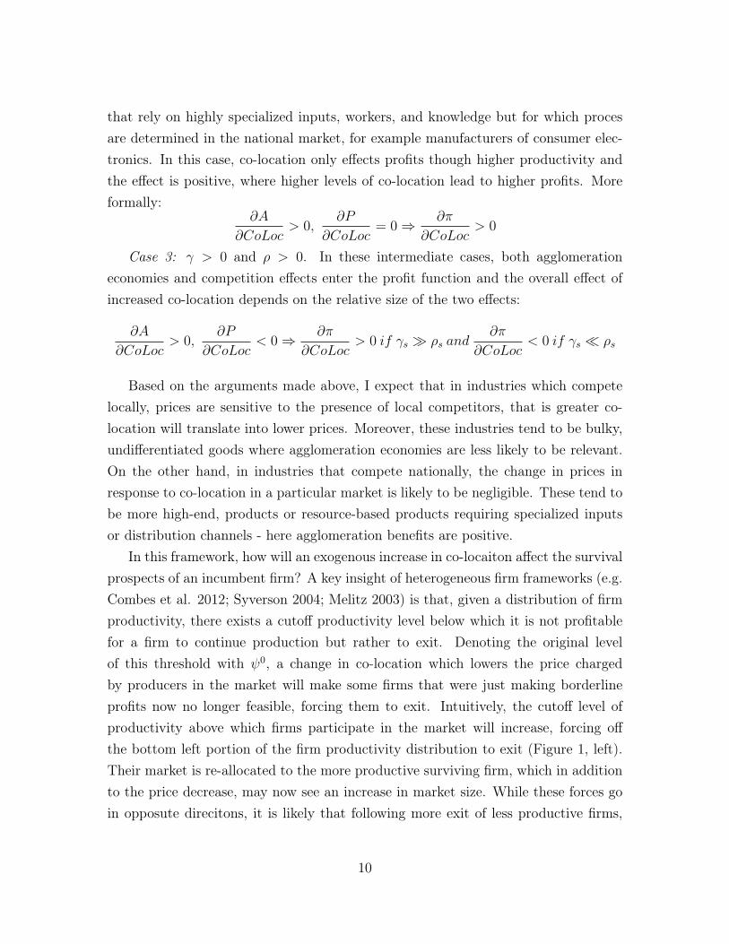
Based on the arguments made above, I expect that in industries which competelocally, prices are sensitive to the presence of local competitors, that is greater co-location will translate into lower prices. Moreover, these industries tend to be bulky,undifferentiated goods where agglomeration economies are less likely to be relevant.On the other hand, in industries that compete nationally, the change in prices inresponse to co-location in a particular market is likely to be negligible. These tend tobe more high-end, products or resource-based products requiring specialized inputsor distribution channels - here agglomeration benefits are positive.

In this framework, how will an exogenous increase in co-locaiton affect the survivalprospects of an incumbent firm? A key insight of heterogeneous firm frameworks (e.g.Combes et al. 2012; Syverson 2004; Melitz 2003) is that, given a distribution of firmproductivity, there exists a cutoff productivity level below which it is not profitablefor a firm to continue production but rather to exit. Denoting the original levelof this threshold with ψ0, a change in co-location which lowers the price chargedby producers in the market will make some firms that were just making borderlineprofits now no longer feasible, forcing them to exit. Intuitively, the cutoff level ofproductivity above which firms participate in the market will increase, forcing offthe bottom left portion of the firm productivity distribution to exit (Figure 1, left).Their market is re-allocated to the more productive surviving firm, which in additionto the price decrease, may now see an increase in market size. While these forces goin opposute direcitons, it is likely that following more exit of less productive firms,

10

the surival prospects of the most prodcutive firms will increase due to the market sizeeffect. These expected dynamics in locally traded industries lead to the following twohypotheses:

Hypothesis 1 : In locally traded industries, an increase in co-location will lead toincreased exit of the least productive firms.

Hypothesis 2 : In locally traded industries, an increase in co-location will improvethe survival prospects of the most productive firms.

Meanwhile, a change in co-location which increases the productivity of all localfirms through higher TFP but is not reflected in product process (which may bedetermined by a much larger number of firms beyond the local market), has theeffect of facilitating the survival of all firms in the local market. Visually, it canbe represented as a shift in the entire distribution of firm productivities to the right(Figure 1, right). These dynamics in nationally traded industries leads to the followingtwo hypotheses:

Hypothesis 3 : In nationally traded industries, an increase in co-location will im-prove firms’ survival prospects.

3 Data and Measurement

3.1 Measuring Co-Location

Two standard ways to measure co-location are used in the literature. Both count thenumber of firms (or workers) located the same industry as the focal firm and pre-defined geographic area. Differences arise in the choice of geographic area. While dis-crete measures count all firms in the same administrative unit (e.g. state or county),continuous measures use spatial distance bands (e.g. 10km, 50km) without regard foradministrative boundaries, normalizing the count by the distance to the focal firm(Rosenthal and Strange 2003, Sorenson and Audia 2000; Haveman and Rider, 2014).The second approach is more representative of real-world interactions, which do notmake a full stop at administrative boundaries. There is no consensus in the literatureon what the “right” geographic distance over which to generate the count is; ratherit depends on the economic interactions that the researcher is interested in (Alcácerand Zhao 2016).

In this paper, I follow the second approach but with two important refinements.

11

First, I use a geographic definition of market that is independent of administrativeboundaries, defining local markets “organically” as all of the destinations that a firmcan reach in four hours traveling on local roads. I choose four hours because of itspractical significance as the destinations that can be reached with one working day(including the return trip), keeping in mind relatively strict regulations regarding 8-hour working days for truckers in Brazil. Figure 2 shows examples of markets arisingfrom this definition. Second, rather than depreciating the count of each firm by itsstraight-line distance to the focal firm, I leverage time-travel time data to generatea measure that better incorporates the actual travel possibilities and costs betweenlocations. Specifically,

CoLocsmit = ln

(∑j∈s,M

xjtτmk

)is the co-location of firm i at time t in industry s and municipalitym, xjt is the variablebeing counted (firm j at time t), τmk is the travel time between municipalities m andk, and M is firm i’s local market defined as all of the destinations which are no morethan four hours apart from municipality m by road i.e. τmk≤ 240 minutes.3 Becausea small number of firms have zero own-industry firms in their four-hour radius, I add0.1 to the raw measure before taking logs.

3.2 Firm-Level Data

Firm level data comes from the Relação Annual de Informações Sociais (RAIS) a high-quality employer-employee matched database that provides an annual census of allformal-sector firms in Brazil. I aggregate the employee-level data to the establishmentlevel using each establishment’s unique ID to create an establishment-level paneldataset.4 I restrict the sample to firms active in manufacturing during the entire

3Because I don’t observe within-municipality travel times, for any pair of firms that are locatedin the same municipality, I set the travel time equal to 15 min. The average size of a municipalityin Brazil is roughly 1,500 sq. km. Assuming municipalities take the shapes of a square, one cancalculate the expected distance between two randomly chosen points to be roughly 20km, whichtranslates into 15 minutes driving time at a speed of 80 km per hour.

4When aggregating the employee-level data to the establishment level, an establishment canbecome associated with more than one record in the same year due to differences in the employee-level data in field values for industry, legal form, municipality, etc. In such cases, I select the modalsample, meaning the record associated with the largest number of employee contracts. I further cleanthe data by removing establishments with invalid IDs, all CEI entities which are multi-jurisdictionentities primarily associated with the construction sector, and all organizations that were not a

12

period with a minimum size of three workers over the 2007-2014 period.5 I dropindustries which may be directly affected by road construction, industries with fewerthan ten firms active in the baseline year 2007, and three industry categories that aretoo general to be meaningful for identifying competition or agglomeration forces.6 Inthe analyses of firm performance outcomes (but not in the measure of co-location), Ialso exclude all companies with state ownership or control to lessen concerns aroundspecial treatment of such companies and establishments belonging to multi-unit firmswhich make up around 7 percent of manufacturing establishments in Brazil. For multi-unit firms other mechanisms may be at play, relating to their internal organizationand agglomeration dynamics (Alcácer and Delgado 2016).7 Given this exclusion, allfirms in the baseline sample are single-establishment firms.

The analysis will examine the survival dynamics of incumbent firms in this samplefrom 2007-2014.8 To do so, I define 2007 incumbents as all firms that existed at thestart of 2007, i.e. those that entered in year 2006 or earlier. This baseline sampleconsist of close to 130,000 firms with an average size of 23 workers. Each firm inthe sample is identified with a unique 4-digit industry and municipality in each year,representing 252 industries and 3,724 municipalities in total. Table 1 shows descriptivestatistics of the firms in the sample.

3.3 Road Network Data

I combine three data sources to construct the time-varying geospatial road networkthat will be used to derive travel times between all Brazilian municipalities in 2007and 2014. Geo-referenced data on the location of municipal capitals and on the federal

business entry during the entire period.5Firms in manufacturing industries are identified using information on the industry code reported

by each establishment. In the Brazilian industry classification system, Classificação Nacional deAtividades Econômicas (CNAE) version 1.0, manufacturing industries fall in 2-digit sectors 15-37.For more detail, see http://biblioteca.ibge.gov.br/visualizacao/livros/liv2314.pdf.

6The seven industries excluded due to the first criterion are manufacturing of concrete (2630),stone (2691), cement (2691), construction bulldozers (2953), construction equipment (2995), earth-moving and paving equipment (2954) and heavy military equipment manufacturing (2972). Thethree excluded due to the second criterion are industries relating to chemical products, machinerepair, and motor vehicle parts containing “not elsewhere specified” in the industry name.

7Note that both types of establishments (state-owned and multi-unit firm) are included in thecalculations of all economic variables, including co-location, as these firms do affect the local com-petitive and agglomerative dynamics.

8I exploit the 2000-2007 period of the data to control for pre-trends.

13

and state transportation network come from the Brazilian Ministry of Transportation(MoT) which developed detailed databases of the Brazilian logistics network as partof the National Logistics and Transport Plan (PNLT) in 2009.9 The PNLT maprepresents the condition of the federal and state road network in 2009 and it detailsthe spatial location, length, and surface type of the more than 18,000 distinct roadsegments with a total length of more than 280,000 kilometers that comprise theBrazilian federal and state road network.

I match data from two additional sources to the 2009 PNLT geo-spatial roadnetwork map in order to reconstruct the condition of the road network in 2007 (prePAC program) and 2014 (post program). One is data from the federal governmentdepartment in charge of transport infrastructure (DNIT) that shows the surface type(e.g. duplicated, single-lane, dirt, etc.) for of each road segment at every year-end.Using this data, I construct the surface of the network in 2007 and 2014.10 Table 2shows the percentage of the federal road network in each surface type in 2007 and2014.11

The second is data on the condition of the road surface (excellent, good, regular,bad, very bad) which comes a physical survey of all major Brazilian roads conductedannually by the Brazilian National Transport Confederation (CNT).12 In 2007, theCNT surveyed more than 92,000 kilometers of the federal and state road network andassigned one of five indicators of surface condition. I digitized the 2007 and 2014 dataon surface conditions from the CNT and geo-referenced it to match the PNLT map.13

9The PNLT data were downloaded from http://www.transportes.gov.br/conteudo/2822-base-de-dados-georreferenciados-pnlt-2010.html. Prior studies that use this data include Schettini andAzzoni (2014) and de Carvalho et al., (2016).

10The annual data on road segment conditions are available fromhttp://www.dnit.gov.br/sistema-nacional-de-viacao/. These are matched to the geo-spatialPNTL data using the segment identifier (SNV/PNV codigo). Note that the segment identifier forsome segments changes over time. Therefore I first match all segments on the segment identifierand length. For the remainder, I perform a geo-spatial matching technique. The final translationfile matching 2007 codes to 2014 codes is available from the author upon request.

11Note that because data on the current surface is only available for federal road segments,I assume that the surface type of the state roads remains unchanged during the time period ofanalysis. This simplifying assumption is unlikely to create large distortions in the measures asduring the 2007-2014 period, there were few major state-level road investment initiatives.

12The data are available from http://pesquisarodovias.cnt.org.br/Edicoes in pdf format. I dig-itized and geo-referenced these data and matched them to the PNLT segments. These data areavailable from the author upon request.

13Over time, the CNT has increased the extent of the network that is surveys. In order to

14

Table 3 shows the percentage of road segments by surface condition in 2007 and 2014.Overall, the program upgraded the surface type for roughly 6,500 kilometers of roadand improved the surface condition of roughly 25,000 kilometers of road.

Using the information on its surface type and condition, I assign a travel velocityto each road segment. The velocity represents the likely actual speed of a truckdriving on that road segment, rather than the speed limit. My assumptions of travelvelocities for given road surfaces and conditions (Table 4) are based on discussionswith the Brazilian Ministry of Transport and leading Brazilian transport economists.The changes in travel velocity of the road segments, which stem from changes in theroad surface type and/or condition between 2007 and 2014 are the only drivers of thechanges in travel times that will be used in the analysis.

3.4 Constructing an O-D Matrix of Travel Times

A key input into the analysis are changes in travel times between firm locations thatresult from the road improvements implemented during the PAC program between2007 and 2014. The lowest geographic level at which I identify firm locations in thedata are Brazilian municipalities, which are slightly smaller on average than U.S.counties. I identify each municipality as its main city (sede municipais) and use thisas my definitions of firm location.14 Municipalities represent a finer level spatial unitof analysis than was available in most prior studies of the effects of roads (Faber,2014; Ghani, Goswami, and Kerr, 2015).

I overlay the location of all municipalities onto the geo-referenced road network tocalculate the municipality-to-municipality minimum travel time on the road networkin 2007 and in 2014. These origin-destination (O-D) travel times are calculated usingthe ArcGIS Network Analyst optimal routing tool. Taking each segment’s lengthand velocity as an input, the program solves for the optimal path from each origin

facilitate comparability, I use the CNT quality indicator in our analysis only for those segments thatwere surveyed in both 2007 and 2014. All non-survey roads and those excluded based on the abovecriterion, are assigned a quality of “regular”.

14From time to time, new municipalities are created from one or more existing municipalities.In the 2000-2014 period, just over 50 “new” municipalities were created in Brazil. In order toensure comparability of the concept of municipality over time, I follow prior studies in this context(e.g. Morten and Oliveira 2016) and construct “Minimum comparable areas” or MCAs which is thelowest geographic unit approximating a municipality that is constant since 2000. The 5,565 actualmunicipalities map to 5,478 MCAs. While I use MCAs in all of the empirical analyses, I will continueto refer to them as “municipalities” for simplicity.

15

to each destination that minimizes travel time via Dijkstra’s algorithm, a widelyused algorithm for shortest path problems in graph theory.15 The set of origins anddestinations is formed by taking all municipal capitals that lie within 50 km of astate or federal road.16 The resulting O-D matrix is a roughly 30 million lengthmatrix containing the travel time (in minutes) and travel distance (in kilometers)between all city pairs in 2007 and 2014.17

Comparing the 2007 and 2014 O-D matrix that I derive, I find that over the entirenetwork, the program lowered travel times by roughly 5.2 percent, significantly morethan similar programs recently evaluated (e.g. Gibbons et al. 2017). Since the focusof this study is on changes in local markets, Figure 3 illustrates for each municipalitythe percentage change in the total travel time to all destinations that were reachablewithin four hours in 2007. While the average local travel time decrease is 2 percent,there is significant variation across different regions of the country, with some regionsseeing travel times in local markets fall by more than 15 percent. Finally, some regionssaw a net deterioration in the quality of local road networks, resulting in increases inlocal travel times.

3.5 Verifying O-D Matrix Accuracy via Google Maps

Since all of the variation used in the analysis stems from travel time changes, Iimplement several tests to verify the accuracy of the O-D matrix that the methodologyyields. To do so, I select a one percent random sample of origin-destination pairs fromthe OD matrix (292,040 city-pairs) and query each pair in this sample via GoogleMaps, recording the travel distances and travel times that it returns.18 Despite some

15Other recent papers have used similar techniques to estimate travel times between locations,for example Allen and Arkolakis (2014) and Morten and Olivera (2016) who use the “fast marchingalgorithm”. The FMA is similar to the Dijkstra shortest path algorithm, with the key differencebeing that the FMA can be applied to calculate speeds over continuous graphs (vs. networks) andcan calculate the speeds of three-dimensional surfaces such as waves.

16Out of the 5,565 municipal capitals on Brazil, 5,505 meet this criterion. The majority of themunicipalities that are not included due to this criterion lie in the Amazon region.

17Because there exist some parts of the network that are not connected to the every other city(i.e. some parts of the federal and state network form disconnected clusters) actual length of the ODmatrix is 29.2 million. Specifically, 5,404 cities form the largest fully connected part of the networkwhile the remaining 101 cities form smaller, disconnected clusters.

18The Google Maps queries were conducted in May 2017.

16

expected sources of differences between the estimates,19 the exercise shows that the O-D estimates have a very high degree of overlap with the Google Maps results. Figure4 shows the correlation of the estimated travel distances (in kilometers) and traveltimes (in minutes) between the Google Maps results and the O-D matrix in the year2014 which are 0.98 and 0.97, respectively. The distributions of the two estimatesalso have a very high degree of overlap (Figure 5).20 Specifically, for city pairs lyingwithin four hours from each other or less (which are the distances I employ in thisanalysis) the median discrepancy between the distance estimated by Google Mapsand the O-D matrix is 1.5 kilometers and the median discrepancy in travel times, 11minutes.

In further tests, I regress the residual from a regression of Google Maps travel timeon Google Maps distance on the travel time estimated by the O-D Matrix. While thefirst regression (Google time on Google distance) has a R2 of 0.99, the results of thisexercise show that the O-D matrix travel times have significant power to predict theresidual variation. Specifically, a regression of the residual component on the O-Dmatrix travel time has an R2 of 0.3 with a t-statistic of 127.7. This second tests alsoconfirm that the O-D matrix measures are meaningful signals of true real-world traveltimes.

3.6 Locally and Nationally Traded Industries

The most direct way to identify which industries trade locally versus nationally wouldbe to observe the actual patterns of internal trade in different industries. In theUnited States, the Commodity Flow Survey (CFS), a survey of the movement of goods

19There are several reasons why I do not expect the estimates to fully overlap with the GoogleMaps estimate. One is that the OD matrix ignores the existence of local (municipal) roads, whilethese are taken into account in Google Maps. Second, Google Maps takes into account historicaldata on traffic congestion, while my estimates do not. Both of these reasons are likely to leadGoogle Maps to predict longer travel times than the OD matrix. There are also reasons that GoogleMaps would predict shorter times and distances and these include: i) The Google Maps query willincorporate any additional improvements in road conditions that took place between 2014 and 2017;ii) Google Maps will include the possibility of travel via ferry (i.e. not only via roads); and iii)Google Maps assumes velocities for a light vehicles (cars) while my velocity assumption reflects thelikely speed of trucks.

20Manual checks suggests that the tendency of the OD measure to have a higher density at highvalues of distance relative to the Google Maps measure tends to relate to the possibility of travelon river routes, which are usually not included in the OD analysis. This problem is less likely to berelevant in within local market travel, which is the focus of this paper.

17

collected every five years, provides information on the distances at which goods areshipped for a selection if industries in manufacturing, mining, wholesale, and selectedretail and services establishments. Even at the very broad sector groupings providedin the publicly accessible data, we see large differences across sectors in how far goodsare traded. For example, the median shipment distance for resource-based products,beverages, food, fabricated metals, wood products and paper products shipped ontrucks is less than 200 miles, a radius of roughly two to four hours. Meanwhile themedian distance a product in machinery, computer products, electrical equipmentand apparel is shipped by truck is more than 500 miles (Figure 6). Thus while theformer products are deemed locally traded, the later are nationally traded.

In the absence of internal trade data, studies have classified manufacturing in-dustries as locally or nationally traded following the principle that nationally tradedindustries concentrate production in a few locations while locally-traded or no-tradedindustries are found everywhere (Delgado, Porter, and Stern 2015; Mian and Sufi2014). I follow this second principle and use data on the actual industry locationpatterns in Brazil from RAIS to classify industries as nationally or locally traded.To do so I calculate, for each industry the Ellison-Glaeser index, a well-known mea-sure of the spatial concentration of industries which counts the share of an industry’semployment in a geographic unit (e.g. county) and compares it to the share of theindustry’s employment nationally, while adjusting for the industry Herfindahl indexto account for concentrations that are due to the industry simply having few firms.Industries with an index value above zero then exhibit grater geographic concentra-tion than economic activity overall, while those with a value below zero concentrateless than expected if they followed the overall distribution of economic activity.

I employ the cutoffs used in Ellison and Glaeser to categorize industries as highlyconcentrated or not highly concentrated to classify industries as nationally or locallytraded. Specifically, industries with index values above 0.05 and below 0.02 are clas-sified as nationally and locally traded, respectively. This procedure yields 73 locallytraded and 99 nationally traded industries. Looking at the largest industries in termsof the number of firms represented in the sample (Table 5), the locally traded sam-ple includes a number of relatively undifferentiated, transport cost intensive products(metal frames, ice cream manufacturing, bakeries, dairy, wooden articles, etc.) whilethe nationally traded sample features more differentiated industries (cosmetics, elec-tronic materials, machine tools, etc.).

18

4 Identification Strategy and Institutional Context

Empirical research on the links between co-location of firms and their performanceconfronts a number of challenges. The following section describes the advantagesand assumptions inherent in the use of road upgrades for identification of causalrelationships. I discuss the institutional setting and the methodology used to generatea measure of exogenous variation in co-location.

4.1 Identification Strategy

The current empirical literature on the effects of co-location on firm performance hasstruggled to address two key sources of bias. One is selection bias created by endoge-nous sorting of firms to locations. If a priori higher quality firms select themselvesinto more (or less) competitive markets, we could see a positive (negative) relationshipbetween proximity to competitors and firm performance even in the absence of anycausal effects. We indeed have strong evidence that selection exists (Shaver and Flyer2000, Kalnins and Chung 2004). A second concern stems from the incorporation ofthe local dynamics of firm entry, exit, and growth in calculating changes in agglomer-ation. If unobserved local variables (e.g. location- or industry specific shocks) affectat the same time firm entry, exit and growth as well as the performance of the focalfirm, then the estimates would be biased.

One way to deal with selection bias is by using panel data (Baum and Mezias1992, Sorenson and Audia 2000, Henderson, 2003), which allows for the analysis ofchanges in firm level outcomes as a function of changes in the degree of co-location.Panel data can largely control for selection bias through the use of first-differencedor panel regressions with firm fixed effects. However, the second concern has provenharder to address with standard econometric methods and calls for the use of in-struments or natural experiments (Combes, Duranton, and Gobillon 2011). Strongtime-varying instruments for agglomeration, however, are difficult to find and mostexisting solutions rely on the use of lagged levels of agglomeration as instrumentsfor future changes (e.g. Martin, Mayer, and Mayneris 2011). This instrument tendsto be predictive but still suffers from endogeneity if the effects of agglomeration aredynamic, as we have reason to believe.

In this paper I use changes in travel times between firm locations caused by roadupgrades as an exogenous source of variation in co-location. The key advantage of

19

this approach is that it is free of both selection bias and unobserved heterogeneitybecause it does not incorporate any information on the changes in the compositionor growth of firms. Specifically, I define change in co-location as:

4CoLocsmi,07−14 = ln

( ∑j∈s,M14

xj,07τmk,14

)− ln

( ∑j∈s,M07

xj,07τmk,07

)(1)

Note that the measure sums over only the incumbent firms and in 2007 (includingthose with did not survive) and thus does not incorporate the endogenous entry, exit,growth and decline of firms in the market. The only variation in the change in co-location measure stems from i) the variation in travel times between 2007 incumbentsdue to the road upgrades, i.e. differences in τmk,14 and and ii) any changes in the sizeof the local market M that are due to road upgrades. I take a difference of thelogged values of 2014 and 2007 co-location, because this measure has the benefit ofapproximating percentage differences (for small enough changes such as here) whilebeing easily interpretable in a regression.

The use of changes in travel times for exogenous variaiton in co-location is mo-tivated by the view that the mechnisms underlying the effects of co-location - i.e.competitive dynamics and agglomeration spillovers - are in fact sensitive to actualcosts and patterns of mobility rather than only distance per se. Indeed, we haverecent evidence for the view that changes of the road network affect price competi-tion (Asturias et al. 2015, Gross 2016), labor flows (Morten and Oliveira 2016), andknowledge flows (Agrawal, Galasso, Oettl 2016).

4.2 Institutional Context

The setting of this study is Brazil during the 2007-2014 period. This is an interestingsetting for a number of reasons. One is its economic relevance as the world’s 7thlargest economy (IMF, 2016) and the fourth largest recipient of FDI inflows amongemerging economies (UNCTAD, 2016). The trend of a growing share of the world’seconomic activity shifting towards emerging markets calls a better understandingof the ways in which institutional differences across locations affect firm strategyand firm performance (Ricart et al. 2004; Khanna and Palepu, 2010). Second, thelack of quality infrastructure, which is a feature of many emerging markets due to

20

their underdeveloped institutions (Henisz 2002), is especially pronounced in Brazil.21

Brazil therefore offers an excellent setting for understanding to what extent a releaseof this constraint changes the nature of competitive interactions as well as potentialfor positive externalities among firms.

This study leverages the Programa de Aceleração do Crescimento (“PAC”), a gov-ernment investment program which took place during 2007-2014.22 It invested morethan 70 billion reals (roughly 35 billion dollars) and upgraded roughly 19,000 kilome-ters of federal roads. Unlike road investment programs that took a holistic approach,23

the Brazilian program was highly decentralized, with more than 250 different road in-vestment projects taking place across different parts of the network. The main statedaim of the program to relieve key constraints in the network. Anecdotal evidencepoints to the view that the program was especially sensitive to constraints faced bythe country’s agricultural exporters (especially soy and corn) seeking to connect toprocessing facilities to ports of export. Practically all investments were upgradesrather than new road construction. While some investments served to upgrade theroad surface type (e.g. paving a dirt road) others improved the surface condition(e.g. repaving, filling pot holes, signaling) to improve the performance and capacityof existing roads.

An important concern is that the allocation of road upgrades to particular regionsmay be correlated with the expected performance of the local firms. This is a validconcern because spurring economic growth in certain regions is often a driver of in-frastructure investment decisions. I address the endogenous road placement concernwith the inclusions or a rich set of industry- and municipality- fixed effects in the em-pirical analysis. Specifically, all regressions include dummy variables for the roughly250 industries and then more than 3,000 municipalities represented in the sample.These control for potential biases that would arise if the government targeted roadinvestments toward particular industries throughout the country or specific munici-

21Brazil ranks 123rd out of 144 countries on the World Economic Forum’s “Quality of overallinfrastructure” index, well behind China (51st) and India (74th). Surveyed executives cite an inad-equate supply of infrastructure as the fourth most problematic factor for doing business, after taxrates, restrictive labor regulations, and corruption.

22Source: http://www.pac.gov.br/. The statistics refer to Phases I and II of the program whichtook place during 2007-2014. Phases III and IV are ongoing.

23For example China’s National Trunk Highway Development Program whose stated objectiveswere to connect all major provincial capitals and cities (Faber, 2014) or the Golden QuadrilateralProject which connects the four major cities in India (Ghani, Goswami, and Kerr, 2015).

21

palities that were expected to perform well (or poorly). Note that the inclusion ofthese fixed effects place a significant hurdle on the empirical analysis, as these fixedeffects alone consume three quarters of the variation in the change in co-locationmeasure (R2=0.75).

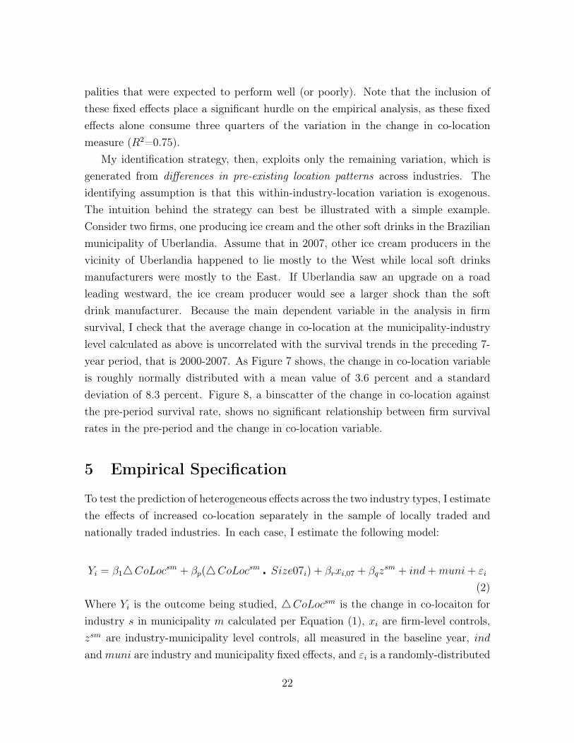
My identification strategy, then, exploits only the remaining variation, which isgenerated from differences in pre-existing location patterns across industries. Theidentifying assumption is that this within-industry-location variation is exogenous.The intuition behind the strategy can best be illustrated with a simple example.Consider two firms, one producing ice cream and the other soft drinks in the Brazilianmunicipality of Uberlandia. Assume that in 2007, other ice cream producers in thevicinity of Uberlandia happened to lie mostly to the West while local soft drinksmanufacturers were mostly to the East. If Uberlandia saw an upgrade on a roadleading westward, the ice cream producer would see a larger shock than the softdrink manufacturer. Because the main dependent variable in the analysis in firmsurvival, I check that the average change in co-location at the municipality-industrylevel calculated as above is uncorrelated with the survival trends in the preceding 7-year period, that is 2000-2007. As Figure 7 shows, the change in co-location variableis roughly normally distributed with a mean value of 3.6 percent and a standarddeviation of 8.3 percent. Figure 8, a binscatter of the change in co-location againstthe pre-period survival rate, shows no significant relationship between firm survivalrates in the pre-period and the change in co-location variable.

5 Empirical Specification

To test the prediction of heterogeneous effects across the two industry types, I estimatethe effects of increased co-location separately in the sample of locally traded andnationally traded industries. In each case, I estimate the following model:

Yi = β14CoLocsm + βp(4CoLocsm � Size07i) + βrxi,07 + βqzsm + ind+muni+ εi

(2)Where Yi is the outcome being studied, 4CoLocsm is the change in co-locaiton forindustry s in municipality m calculated per Equation (1), xi are firm-level controls,zsm are industry-municipality level controls, all measured in the baseline year, indandmuni are industry and municipality fixed effects, and εi is a randomly-distributed

22

error term.I estimate the model as a linear probability model (LPM) using ordinary least

squares (OLS) due to the large number of fixed effects, which make a logit modelcomputationally intensive.24 In the simplest model, β1 provides the estimate of theaverage effect of co-location on firm survival. However, in order to test the theoreticalprediction of heterogenous effects across more and less productive firms, I includeinteraction terms for the change in co-location and proxies for productivity that arebased on firm size in 2007.25 The first proxy is the simple measure of size (workers),Size07i. As other proxies, I calculate different quantiles of firm size for each focalfirm relative to all other firms in its industry, as well as relative only to firms in itsindustry and local market. In models that include the interactions of the co-locationshock with firm size, β1 shows the effect for the omitted category (usually the smallestfirms) while βps estimate the effects for the other firm categories.

5.1 Dependent Variable

The main dependent variable, Yi, is firm survival over the 7-year period from 2007-2014. The advantage of this variable is that is most closely captures the theoreticalmechanisms described in the models of spatial competition and firm selection wherebythe least productive firms exit. Therefore firm survival is the natural empirical out-come to be tested. I define the variable Survive as an indicator taking the value 1 if a2007 incumbent firm continues to exist in the same municipality and 4-digit industryin 2014 and a value of zero otherwise. Among the firms in the sample, the average7-year survival rate is 55.6 percent - just over half of all firms. Arguably survivalis a much cruder measure of the productivity growth theorized in the agglomerationliterature where a more appropriate theory-backed measure would be residual TFPor value added.26 I use firm survival as the primary proxy of productivity growth,

24Beyond allowing for the large number of fixed effects, the second advantage of the LMP in thiscontext is the ease of interpretation of the estimated coefficients. The main downside is the possibilityof estimated probabilities outside the [0,1] interval. I have checked that estimated probabilitiesoutside the meaningful ranges are rare.

25A strong positive relationship between firm size and productivity of manufacturing firms is welldocumented, for example in Haltiwanger, Lane, and Spletzer (1999).

26Unfortunately, the data required to estimate TFP are not readily available for the cross-sectionof manufacturing firms in Brazil. In addition, TFP estimation has to confront numerous challenges,for example endogenous input choice. As a result, the agglomeration literature has in the pastresorted to the use of employment growth as a productivity proxy, for example in Glaeser el al.

23

assuming that if firms are becoming increasingly productive they also are more likelyto survive.

5.2 Controls

The baseline specifications include three types of controls: firm level, municipalitylevel, and municipality-industry level controls. All are measured in the baseline year,2007 and included in log-form. Table 6 in the Appendix shows the correlations be-tween the main variables.

Firm level controls : I control for firm size (workers) and firm age cohorts. Largerand older tend firms have higher survival rates and may have more power to attractpreferential policies from the government. I also control for three other firm charac-teristics that are likely to be correlated with performance and which may make firmsmore likely targets of government policies. These are the firm’s average worker wage(in reals), and dummies for whether the firm is an exporter or importer.

Municipality-industry level controls : All regressions control for the baseline levelof a firm’s co-location in 2007 for two reasons. One is that the baseline-level of co-location may be correlated with unobserved firm characteristics due to better firmssorting into more or less competitive locations or because more or less competitivelocations result in more productive firms (e.g. though selection). Second, the baselinelevel of co-location is mechanically correlated with the change in co-location becauseof convergence effects (relative changes are smaller from a larger baseline). I alsocontrol for urbanization economies, measures as a count of firms in the focal firm’slocal market but outside it’s industry. Finally, I include a control for competition inthe market-industry (measured as the inverse of the standard Herfindahl index) inorder to control for any potential correlation between the change in co-location andtrends in industry consolidation.

Industry fixed effects : All regressions include industry fixed effects in order tocontrol for any potential correlations coming from macro-level industry shocks orthe possibility that the government targeted road investments to specific industriesthroughout the country based on their expected future performance.

Municipality fixed effects : Finally, all regressions also include fixed effects for eachof the more than 3,000 municipalities. These control for all unobserved characteristics

(1992) and Henderson et al. (1995).

24

that affect the performance of manufacturing firms in the municipality during the2007-2014 period equally (e.g. local shocks), and the possibility that the governmenttargeted investments to certain well-preforming (or poorly-performing) regions.

6 Results

6.1 Co-Location and Survival in Locally Traded Industries

Table 7 shows the results of estimating the model in locally traded industries. Thetop rows show the main coefficients of interest, those on the change in co-locationand its interaction with the productivity proxies (firm size and size quantiles). Ininterpreting the magnitude of the coefficients, β ∗ 100 is the effect of a doublingin co-location (because change in co-location is a log difference, comparable to apercentage change). All non-categorical independent variables enter in log form,hence their coefficients can be interpreted as the estimated effect of a percentagepoint increase in the independent variable on the probability of survival, holding theother variables constant. All specifications include firm level controls in the baselineyear, the industry-municipality, industry- and municipality fixed effects. Standarderrors are clustered at the industry-municipality level to account for the fact that theco-location measure varies at that level.

The simple relationship between the change in co-location and firm survival islarge and negative but not statistically significant in Column (1). Taken at face valuethe coefficient size suggests that a doubling in co-location leads to a 9.1 percentagepoint lower probability of survival, an elasticity of roughly 1/10.

Column (2), in a first test of the prediction of heterogeneous firm-level effects,interacts the change in co-location with firm size. The coefficient on the change inco-location variable is now large, negative, and significant and the interaction effectis positive and highly significant. These results provide the first evidence that theeffect of co-location is heterogeneous in firm size in locally traded industries.

Columns (3)-(5) report the results of the non-parametric model, interacting thechange in co-location with progressively more granular quantiles of a firm’s size in itsindustry. In each case the coefficient on the change in co-location, which measuresthe effect for the smallest firms (omitted category), is large, negative, and significant.Its size implies that a doubling of co-location reduces the survival probability of the

25

smallest firms between 12 and 16 percentage points. Meanwhile, the coefficients forthe larger quantiles are positive and significant, and roughly equal in size, suggestingno, or small, negative effects on survival for the biggest firms.

Column (6), where the quantiles are measured relative only to other firms in thefocal firm’s industry and market, provides evidence that the largest firms in the marketactually gain. The marginal effects of this model suggest that doubling co-location,reduces the survival probability of the smallest firms by 14.1 percentage points andincreases the survival rate of the largest firms by 2.6 percentage points.

Beyond the theorized effects, the coefficients of other variables in the model con-form to expectations. Firm size and age wage have a positive and significant rela-tionship with survival. The coefficient on firm size suggests that a doubling in firmsize is associated with a roughly 6 percentage point higher survival rate. Higheraverage wages are also predictive of higher survival while exporters and importersare, somewhat surprisingly, no more likely to survive in the baseline regression thannon-trading firms. The effects of urbanization economies appear as positive and sig-nificant, suggesting more economic activity outside the own industry is associatedwith a higher survival rate, while the coefficients on the baseline levels of co-locationand competition in the market and industry are small and not statistically significant.

Overall, the results point to significant, negative effects of increased co-location onthe smallest firms in locally traded industries, lending support for Hypothesis 1. Theresults in column (6) also lend support for Hypothesis 2, showing positive effects ofincreased co-location for the largest firms in locally traded industries. Combined theresults provide evidence of selection and reallocation among firms in the same localmarket and industry.

6.2 Co-Location and Survival in Nationally Traded Industries

Table 8 shows the parallel results for nationally traded industries. The coefficients onall the control variables are similar and therefore only the main results are presented.The differences in the main results are striking. In nationally traded industries, thebaseline effect of a change in co-location on firm survival is positive, significant, andlarge. The coefficient in Column (1) suggests that in nationally traded industries,a doubling of co-location increase the survival rate by 14.9 percentage points, onaverage. Column (2), which interacts the shock with firm size, shows a negative but

26

not statistically significant effect, providing weak evidence that the positive effect issmaller for larger firms. This conclusion is again confirmed in columns (3)-(6) whereacross the specifications, the results support the conclusion that doubling co-locationincreases the survival rate of the smallest firms by 18 to 20 percentage points. Thecoefficient on the interaction effects for the larger firms continue to be negative but,due to large standard errors, not statistically significant. The coefficients on thecontrol variables in this sample are similar to those in the locally traded sample.

The baseline results provide significant evidence of large, positive effects of in-creased co-location in nationally traded industries, with no significant differencesacross the firm size distribution. Firms of all sizes benefit from increased proxim-ity in locally traded industries. These results lend significant support for Hypothesis3.

6.3 Relocations and Product Switches

In this section, I investigate whether firms react strategically to changes in co-location.A firm facing increased competition in its product and local market can respondby repositioning (Gimeno, Chen, and Bae 2006, Wang & Shaver 2014) for exampleby changing location or switching products. Given that they face the more seriouscompetitive threats, I expect that the smallest firms in locally traded industries wouldbe most likely to respond to increased co-location by repositioning, relocating to adifferent municipality or switching to a different product. Meanwhile, in nationallytraded industries, increased co-location that increases spillovers makes it less likelythat a firm would more closer toward others in its industry to seek spillovers orresources. Therefore, we should observe fewer moves following an increase in co-location due to the road shock.

In further tests, I analyze product switching and firm relocation. I define thevariable Switch as an indicator taking the value 1 if an incumbent firm reports adifferent industry code in 2007 and in the last year that it is observed in the sample.Similarly, I define the dummy variable Relocate if an incumbent firm is located in adifferent municipality the last year that it is observed.27

I explore these predictions by analyzing whether the prevalence of product switches

27Note that, given the definition of Survive, any firm moving or switching is part of the subset offirms defined as having not survived (in their original location and industry). The main results onsurvival are robust to the dropping of movers and switchers from the sample, i.e. full “exits”.

27

and firm relocations was affected by changes in co-location stemming from the roadupgrades. The model is parallel to Equation (1) but, in addition, the firm levelcontrols now also include a control for the last year that the firm is observed inthe sample, i.e. the year of “exit” (or 2014 in the absence of exit). This control isimportant because time is the main predictor of product switches and relocationsand, as we know from the prior analysis, changes in co-location affect the likelihoodof firms remaining in the sample.

Table 9 shows the results of the analyses of moves and relocations in locally andnationally traded industries. The differences across the two industry types are onceagain impressive and in line with theory. In locally traded industries, the results forthe sample as a whole show that increases in co-location increase the likelihood ofrelocating and switching to a different industry, although the effects are not significantat typical significance levels (Columns 1 and 3). The results become clearer afterintroducing the interactions with firm size quartiles.

For the smallest firms, the likelihood of moving or switching industry increasesas co-location increases. Specifically, doubling co-location increases the likelihoodof moving by 3.8 percentage points and the likelihood of industry switching by 7.4percentage points. Given the average likelihood of moves and product switches of3.1 and 8.4 percent, respectively, this is roughly a doubling of the likelihood of theseevents. Again, larger firms are less likely to move and relocate, through the differencesare not always statistically significant.

In nationally traded industries, on the other hand, the likelihood of moving andswitching industry falls with an increase in co-location. For the smallest firms, dou-bling co-location decreases the probability of moving by 5.2 percentage points, again,more than doubling the baseline probability of 4.1 percent. The coefficients on theinteraction terms suggest that the effect is muted for large firms, though large stan-dard errors render the interaction not statistically significant. The result on switches,which were not clear in theory, is also more ambiguous in the empirical results. Whileall coefficients are negative, suggesting lower propensity to switch industries, none arestatistically significant at the standard thresholds.

A final difference becomes apparent considering the destinations that firms move towhen relocating or switching industries. I calculate, for all firms that move and switchindustry, the difference in co-location between the origin and destination. In Figure 8,we see that firms that relocate or switch industries in locally traded industries tend to

28

move away from competitors, while in nationally traded industries, they move towardcompetitors. While this last piece of evidence is descriptive, it lends support for themain hypothesis of the paper, that proximity to competitors plays a fundamentallydifferent role in nationally traded and locally traded industries.

7 Conclusion

This paper estimates the effect of co-locating with firms in one’s industry on firmsurvival by leveraging reductions in travel times between firm locations stemmingfrom improved roads as exogenous variation in co-location. I find that in industriesthat compete for customers locally, increased co-location produces effects consistentwith heightened competition: doubling co-location lowers the survival rate of thesmallest firm by 14.1 percentage points while increasing it by 2.6 percentage pointsfor the largest firms. In industries that compete in national markets, increased co-location produces effects consistent with increased agglomeration spillovers. Doublingco-location increases firms’ survival rate by 14.9 percentage points, with no significantdifferences across firm sizes. As further evidence, consistent with increased competi-tion in locally traded industries, I observe a higher propensity of firms to move to adifferent municipality or switch their primary product after being brought closer topcompetitors, and when they do so, they evade competition. Meanwhile, in nationallytraded industries I observe fewer relocations and when these occur, they are movestowards competitors.

The findings of significant differences in the way that firms respond to co-locationwith competitors suggest that there is not a single answer to the question how prox-imity affects performance, but rather that studies need to be careful to consider bothindustry and firm level heterogeneity. While the focus of this study is in establish-ing that first-order dimension of heterogeneity, one limitation that stems from itscross-industry nature is the inability to point to the relevance of specific mechanismsbehind the effects (e.g. spillovers from shred input suppliers versus richer labor pools).These could be evaluated in future work with a narrower scope, e.g. studies in a singleindustry or region.

The ability of the study to detect effects on firm behavior based only on changesto the actual cost of mobility also carries the important implication that “space” isnot a constant but rather is shaped by the costs and patterns of human mobility. This

29

opens up opportunities for further inquiry on how changes in technologies and policiesthat affect the cost of mobility shape the competitive and collaborative interactionsbetween firms.

30

References

Agrawal, A., Galasso, A., and Oettl, A. (2016). Roads and Innovation. Review ofEconomics and Statistics, pages 1–45.

Aitken, B. and Harrison, A. E. (1999). Do Domestic Firms Benefit from DirectForeign Investment? Evidence from Venezuela. American Economic Review,89(3):605–618.

Alcacer, J. (2006). Location Choices Across the Value Chain: How Activity andCapability Influence Collocation. Management Science, 52(10):1457–1471.

Alcacer, J. and Delgado, M. (2016). Spatial organization of firms and location choicesthrough the value chain. Management Science, 62(11):3213–3234.

Alcacer, J. and Zhao, M. (2016). Zooming in: A Practical Manual for IdentifyingGeographic Clusters. Strategic Management Journal, pages 10–21.

Alfaro, L. and Chen, M. X. (2017). Selection and Market Reallocation: ProductivityGains from Multinational Production. American Economic Journal: EconomicPolicy.

Allen, T. and Arkolakis, C. (2014). Trade and the topography of the spatial economy.Quarterly Journal of Economics, 129(3):1085–1139.

Almeida, P. and Kogut, B. (1999). Localization of Knowledge and the Mobility ofEngineers in Regional Networks. Management Science, 45(7):905–917.

Arikan, A. T. and Schilling, M. A. (2011). Structure and Governance in Industrial Dis-tricts: Implications for Competitive Advantage. Journal of Management Studies,48(4):772–803.

Asturias, J., García-Santana, M., and Ramos, R. (2015). Competition and the welfaregains from transportation infrastructure: Evidence from the Golden Quadrilat-eral of India.

Baum, J. A. C. and Haveman, H. A. (1997). Love Thy Neighbor? Differentiationand Agglomeration in the Manhattan Hotel Industry, 1898-1990. AdministrativeScience Quarterly, 42(2):304.

31

Baum, J. A. C. and Mezias, S. J. (1992). Localized competition and organizationalfailure in the manhattan hotel industry, 1898- 1990. Administrative ScienceQuarterly, 37(4):580–604.

Beaudry, C. and Swann, G. M. P. (2009). Firm growth in industrial clusters of theUnited Kingdom. Small Business Economics, 32(4):409–424.

Buciuni, G. and Pisano, G. P. (2015). Can Marshall’s Clusters Survive Globalization?

Buenstorf, G. and Klepper, S. (2009). Heritage and agglomeration: The akron tyrecluster revisited. Economic Journal, 119(537):705–733.

Chandra, A. and Thompson, E. (2000). Does public infrastructure affect economicactivity? Regional Science and Urban Economics, 30:457–490.

Chatterji, A., Glaeser, E., and Kerr, W. (2014). Clusters of Entrepreneurship andInnovation. Innovation Policy and the Economy, 14.1:129–166.

Chen, C. and Steinwender, C. (2016). Import Competition, Heterogeneous Prefer-ences of Managers and Productivity.

Chung, W. and Alcacer, J. (2002). Knowledge Seeking and Location Choice of ForeignDirect Investment in the United States. Management Science, 48(12):1534–1554.

Chung, W. and Kalnins, A. (2001). Agglomeration effects and performance: A testof the Texas lodging industry. Strategic Management Journal, 22(10):969–988.

Combes, P. P., Duranton, G., and Gobillon, L. (2011). The identification of agglom-eration economies. Journal of Economic Geography, 11(2):253–266.

Combes, P.-P., Duranton, G., Gobillon, L., Puga, D., and Roux, S. (2012). TheProductivity Advantages of Large Cities: Distinguishing Agglomeration FromFirm Selection. Econometrica, 80(6):2543–2594.

Delgado, M., Porter, M. E., and Stern, S. (2014). Clusters, convergence, and economicperformance. Research Policy, 43(10):1785–1799.

Delgado, M., Porter, M. E., and Stern, S. (2015). Defining clusters of related indus-tries. Journal of Economic Geography, pages 1–38.

32

Duschl, M., Scholl, T., Brenner, T., Luxen, D., and Raschke, F. (2015). Industry-Specific Firm Growth and Agglomeration. Regional Studies, 49(11):1822–1839.

Ellison, G. and Glaeser, E. L. (1997). Geographic Concentration in U.S. Manufactur-ing Industries: A Dartboard Approach. Journal of Political Economy, 105(5):889.

Faber, B. (2014). Trade integration, market size, and industrialization: Evidence fromChina’s national trunk highway system. Review of Economic Studies, 81(3):1046–1070.

Falck, O., Guenther, C., Heblich, S., and Kerr, W. R. (2013). From russia withlove: The impact of relocated firms on incumbent survival. Journal of EconomicGeography, 13(3):419–449.

Fallick, B., Fleischman, C. a., and Rebitzer, J. B. (2006). Job-Hopping in SiliconValley: Some Evidence Concerning the Microfoundations of a High-TechnologyCluster. Review of Economics and Statistics, 88(3):472–481.

Fischer, J. and Harrington, J. (1996). Product Variety and Firm Agglomeration. TheRAND Journal of Economic, 27(2):281–309.

Flyer, F. and Shaver, J. M. (2003). Location Choices Under Agglomeration Externali-ties and Strategic Interaction. Advances in Strategic Management, 20(September2003):193–213.

Foster, L., Haltiwanger, J., and Syverson, C. (2016). The Slow Growth of New Plants:Learning about Demand? Economica, 83(329):91–129.

Frenken, K., Cefis, E., and Stam, E. (2014). Industrial Dynamics and Clusters: ASurvey. Regional Studies, 49(1):10–27.

Furman, J., Porter, M., and Stern, S. (2002). The determinants of national innovativecapacity. Research Policy, 31(6):899–933.

Ghemawat, P. (2007). Redefining global strategy: Crossing borders in a world wheredifferences still matter. Harvard Business Press, Cambridge, MA.

Ghemawat, P. and Thomas, C. (2008). Strategic Interaction Across Countries andMultinational Agglomeration: An Application to the Cement Industry. Manage-ment Science, 54(12):1980–1996.

33

Gibbons, S., Lyytikäinen, T., Overman, H., and Sanchis-Guarner, R. (2012). NewRoad Infrastructure: the Effects on Firms. SERC Discussion paper, (September).

Gimeno, J., Folta, T. B., Cooper, A. C., and Woo, C. Y. (1997). Survival of theFittest? Entrepreneurial Human Capital and the Persistence of UnderperformingFirms. Administrative Science Quarterly, 42(4):750–783.

Giroud, X. (2012). Proximity and Investment: Evidence from Plant-Level Data. TheQuarterly Journal of Economics, pages 861–915.

Goswami, A. G., Ghani, E., and Kerr, W. R. (2015). Highway to Success: The Impactof the Golden Quadrilateral Project for the Location and Performance of IndianManufacturing. Economic Journal.

Gross, D. P. (2016). The Ties that Bind: Railroad Gauge Standards and InternalTrade in the 19th Century U.S.

Haltiwanger, J. C., Lane, J. I., and Spletzer, J. R. (1999). Productivity Differencesacross Employers: The Roles of Employer Size, Age, and Human. The AmericanEconomic Review, 89(2):94–98.

Hannan, M. T. and Freeman, J. (1977). The Population Ecology of Organizations.

Hasan, S. and Koning, R. (2017). When Proximity May Not Be Destiny: The Roleof Existing Relationships.

Haveman, H. a. and Rider, C. I. (2014). The Spatial Scope of Competition and theGeographical Distribution of Entrepreneurship: Magazine Foundings and theU.S. Post Office. Sociological Science, 1(April):111–127.

Head, K., Ries, J., and Swenson, D. (1995). Agglomeration benefits and locationchoice: Evidence from Japanese manufacturing investments in the United States.Journal of International Economics, 38(3-4):223–247.

Henisz, W. J. (2002). The institutional environment for infrastructure investment.Industrial and Corporate Change, 11(2):355–389.

Hotelling, H. (1929). Stability in competition. The Economic Journal, 39(153):41–57.

34

Jaffe, A., Trajtenberg, M., and Henderson, R. (1993). Geographic Localization ofKnowledge Spillovers as Evidenced by Patent Citations. Quarterly Journal ofEconomics.

Kalnins, A. and Chung, W. (2004). Resource-seeking agglomeration: A study ofmarket entry in the lodging industry. Strategic Management Journal, 25(7):689–699.

Kerr, W. R. and Kominers, S. D. (2015). Agglomerative Forces and Cluster Shapes.Review of Economics and Statistics, 97(4):877–899.

Khanna, T. and Palepu., K. G. (2010). Winning in emerging markets: A road mapfor strategy and execution. Harvard Business Press.

Krugman, P. (1991). Geography and Trade. MIT Press.

Lippman, S. A. and Rumelt, R. P. (1982). Uncertain Imitability: An Analysis ofInterfirm Differences in Efficiency under Competition. The Bell Journal of Eco-nomics, 13(2):418.

Marshall, A. (1920). Principles of Economics. MacMillan, London.

Martin, P., Mayer, T., and Mayneris, F. (2011). Spatial concentration and plant-levelproductivity in France. Journal of Urban Economics, 69(2):182–195.

Martin, X., Salomon, R., and WU, Z. (2010). The Institutional Determinants of Lo-cation Choice: Agglomeration in the Global Semiconductor Industry. Industrialand Corporate Change.

McCann, B. T. and Folta, T. B. (2008). Location Matters: Where We Have Beenand Where We Might Go in Agglomeration Research. Journal of Management,34(3):532–565.

McCann, B. T. and Folta, T. B. (2011). Performance differentials within geographicclusters. Journal of Business Venturing, 26(1):104–123.

McCann, B. T. and Vroom, G. (2010). Pricing Response to Entry and AgglomerationEffects. Strategic Management Journal, 31:284–305.

35

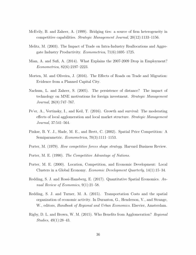
McEvily, B. and Zaheer, A. (1999). Bridging ties: a source of firm heterogeneity incompetitive capabilities. Strategic Management Journal, 20(12):1133–1156.

Melitz, M. (2003). The Impact of Trade on Intra-Industry Reallocations and Aggre-gate Industry Productivity. Econometrica, 71(6):1695–1725.

Mian, A. and Sufi, A. (2014). What Explains the 2007-2009 Drop in Employment?Econometrica, 82(6):2197–2223.

Morten, M. and Oliveira, J. (2016). The Effects of Roads on Trade and Migration:Evidence from a Planned Capital City.

Nachum, L. and Zaheer, S. (2005). The persistence of distance? The impact oftechnology on MNE motivations for foreign investment. Strategic ManagementJournal, 26(8):747–767.

Pe’er, A., Vertinsky, I., and Keil, T. (2016). Growth and survival: The moderatingeffects of local agglomeration and local market structure. Strategic ManagementJournal, 37:541–564.

Pinkse, B. Y. J., Slade, M. E., and Brett, C. (2002). Spatial Price Competition: ASemiparametric. Econometrica, 70(3):1111–1153.

Porter, M. (1979). How competitive forces shape strategy. Harvard Business Review.

Porter, M. E. (1990). The Competitive Advantage of Nations.

Porter, M. E. (2000). Location, Competition, and Economic Development: LocalClusters in a Global Economy. Economic Development Quarterly, 14(1):15–34.

Redding, S. J. and Rossi-Hansberg, E. (2017). Quantitative Spatial Economics. An-nual Review of Economics, 9(1):21–58.

Redding, S. J. and Turner, M. A. (2015). Transportation Costs and the spatialorganization of economic activity. In Duranton, G., Henderson, V., and Strange,W., editors, Handbook of Regional and Urban Economics. Elsevier, Amsterdam.

Rigby, D. L. and Brown, W. M. (2015). Who Benefits from Agglomeration? RegionalStudies, 49(1):28–43.

36

Rosenthal, S. and Strange, W. (2003). Geography, industrial organization, and ag-glomeration. Review of Economics and Statistics, 85(2):377–393.

Rotemberg, J. J. and Saloner, G. (2000). Competition and human capital accumu-lation: A theory of interregional specialization and trade. Regional Science andUrban Economics, 30(4):373–404.

Rumelt, R. (1991). How much does industry matter? Strategic Management Journal,12(3):167–185.

Salop, S. C. (1979). Monopolistic Competition with Outside Goods. The Bell Journalof Economics, 10(1):141–156.

Schettini, D. and Azzoni, C. (2015). Determinantes Regionais da ProductividadeIndustrial: O Papel da Infraestrutura. In Produtividade no Brasil, volume 2,pages 391–415. Instituto de Pesquisa Econômica Aplicada (Ipea) Organizadores.

Schwab, K. (2015). The global competitiveness report 2015-2016, volume 5.

Shaver, M. J. and Flyer, F. (2000). Agglomeration Economies, Firm Heterogene-ity, and Foreign Direct Investment in the United States. Strategic ManagementJournal, 21(12):1175–1193.

Singh, J. and Marx, M. (2013). Geographic Constraints on Knowledge Spillovers:Political Borders vs. Spatial Proximity. Management Science, 59(9):2056–2078.

Sorenson, O. and Audia, P. G. (2000). The Social Structure of Entrepreneurial Ac-tivity: Geographic Concentration of Footwear Production in the United States1940-1989. American Journal of Sociology, 106(2):424–462.

Syverson, C. (2004). Market Structure and Productivity: A Concrete Example. Jour-nal of Political Economy, 112(6):1181–1222.

Vernon Henderson, J. (2003). Marshall’s scale economies. Journal of Urban Eco-nomics, 53(1):1–28.

Vogel, J. (2008). Spatial Competition with Heterogeneous Firms. Journal of PoliticalEconomy, 116(3):423–466.

Wang, R. and Shaver, M. (2014). Competition-Driven Repositioning. Strategic Man-agement Journal, 1604.

37

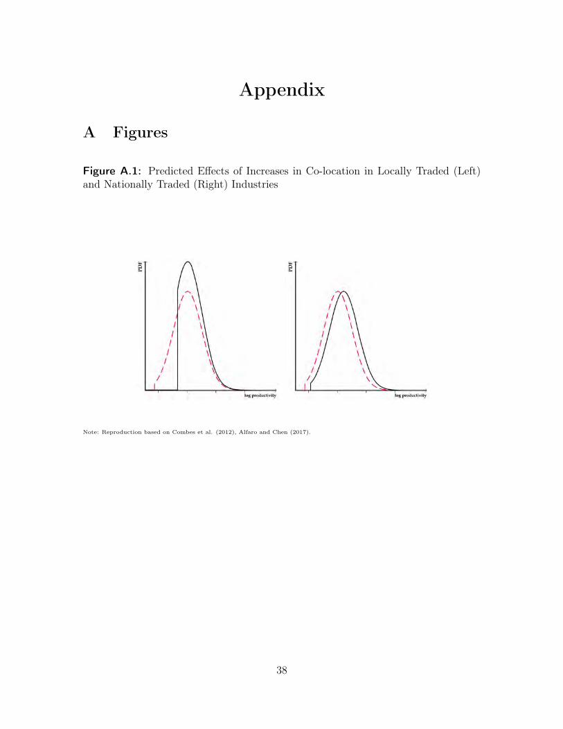
Appendix

A Figures

Figure A.1: Predicted Effects of Increases in Co-location in Locally Traded (Left)and Nationally Traded (Right) Industries

Note: Reproduction based on Combes et al. (2012), Alfaro and Chen (2017).

38

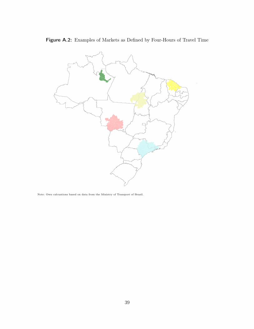
Figure A.2: Examples of Markets as Defined by Four-Hours of Travel Time

Note: Own calcuations based on data from the Ministry of Transport of Brazil.

39

Figure A.3: Change in Local Travel Times Between in Brazilian Municipalities,2007-2014

Note: Own calcuations based on data from the Ministry of Transport of Brazil. Map shows the total percentage change in the averagetime of traveling from each city (sede municipais) to each other city in its local market (a city’s local market is any municipality thatcan be reached in 4 hours or less traveling by federal and state roads in 2007). Areas not shaded (white) are municipalities whosecapital lies more than 50 km away from a state or federal road and are not included in the analysis.

40

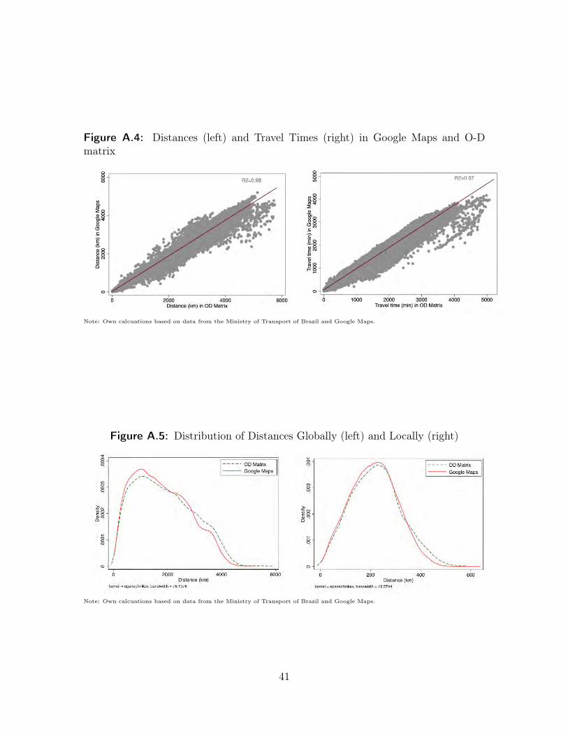
Figure A.4: Distances (left) and Travel Times (right) in Google Maps and O-Dmatrix

Note: Own calcuations based on data from the Ministry of Transport of Brazil and Google Maps.

Figure A.5: Distribution of Distances Globally (left) and Locally (right)

Note: Own calcuations based on data from the Ministry of Transport of Brazil and Google Maps.

41

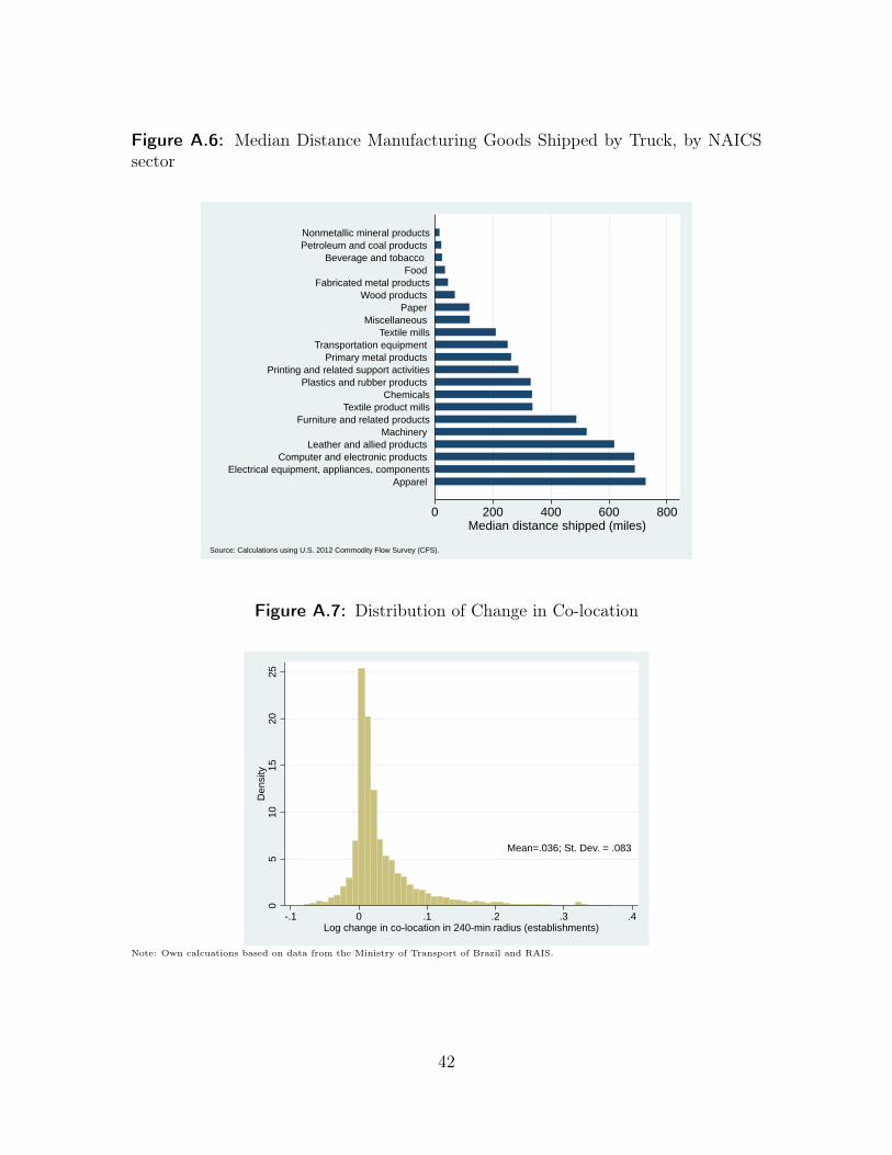
Figure A.6: Median Distance Manufacturing Goods Shipped by Truck, by NAICSsector

0 200 400 600 800Median distance shipped (miles)

Apparel Electrical equipment, appliances, components

Computer and electronic products Leather and allied products

Machinery Furniture and related products

Textile product millsChemicals

Plastics and rubber products Printing and related support activities

Primary metal products Transportation equipment

Textile millsMiscellaneous

Paper Wood products

Fabricated metal productsFood

Beverage and tobacco Petroleum and coal products Nonmetallic mineral products

Source: Calculations using U.S. 2012 Commodity Flow Survey (CFS).

Figure A.7: Distribution of Change in Co-location

Mean=.036; St. Dev. = .083

05

1015

2025

Den

sity

-.1 0 .1 .2 .3 .4Log change in co-location in 240-min radius (establishments)

Note: Own calcuations based on data from the Ministry of Transport of Brazil and RAIS.

42

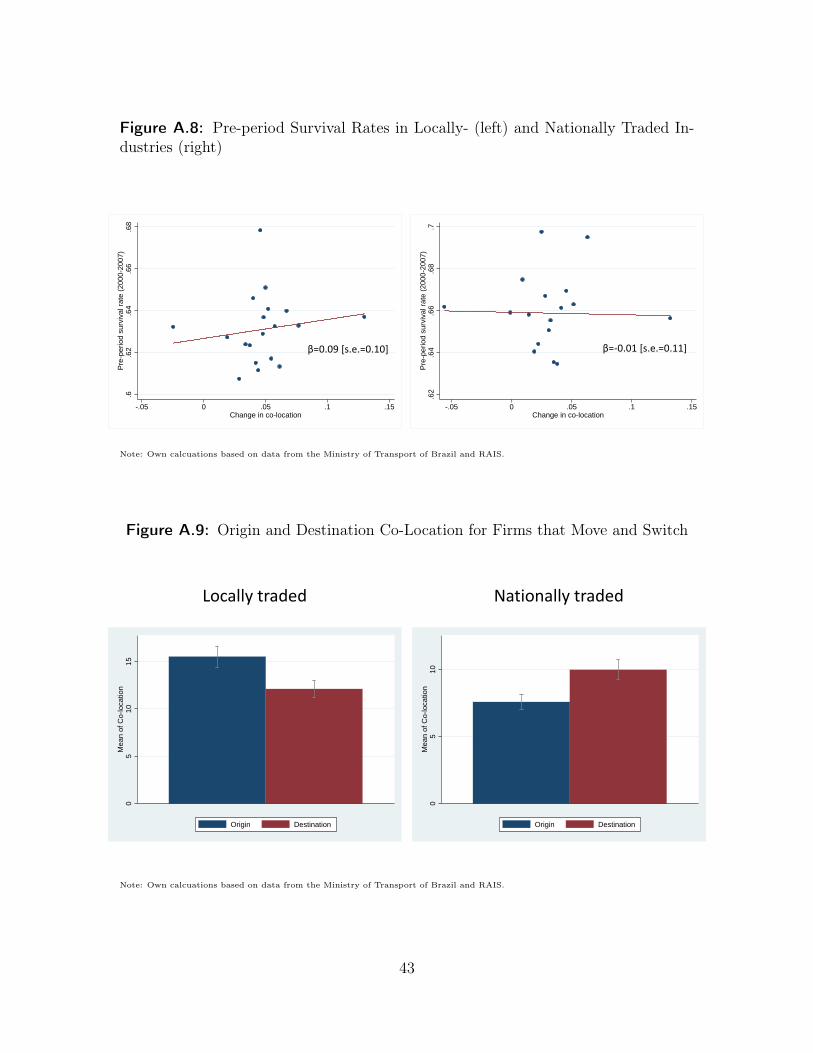
Figure A.8: Pre-period Survival Rates in Locally- (left) and Nationally Traded In-dustries (right)

.6.6

2.6

4.6

6.6

8Pr

e-pe

riod

surv

ival

rate

(200

0-20

07)

-.05 0 .05 .1 .15Change in co-location

.62

.64

.66

.68

.7Pr

e-pe

riod

surv

ival

rate

(200

0-20

07)

-.05 0 .05 .1 .15Change in co-location

β=0.09[s.e.=0.10] β=-0.01[s.e.=0.11]

Note: Own calcuations based on data from the Ministry of Transport of Brazil and RAIS.

Figure A.9: Origin and Destination Co-Location for Firms that Move and Switch

Locallytraded

05

1015

Mea

n of

Co-

loca

tion

Origin Destination

Nationally traded

05

10M

ean

of C

o-lo

catio

n

Origin Destination

Note: Own calcuations based on data from the Ministry of Transport of Brazil and RAIS.

43

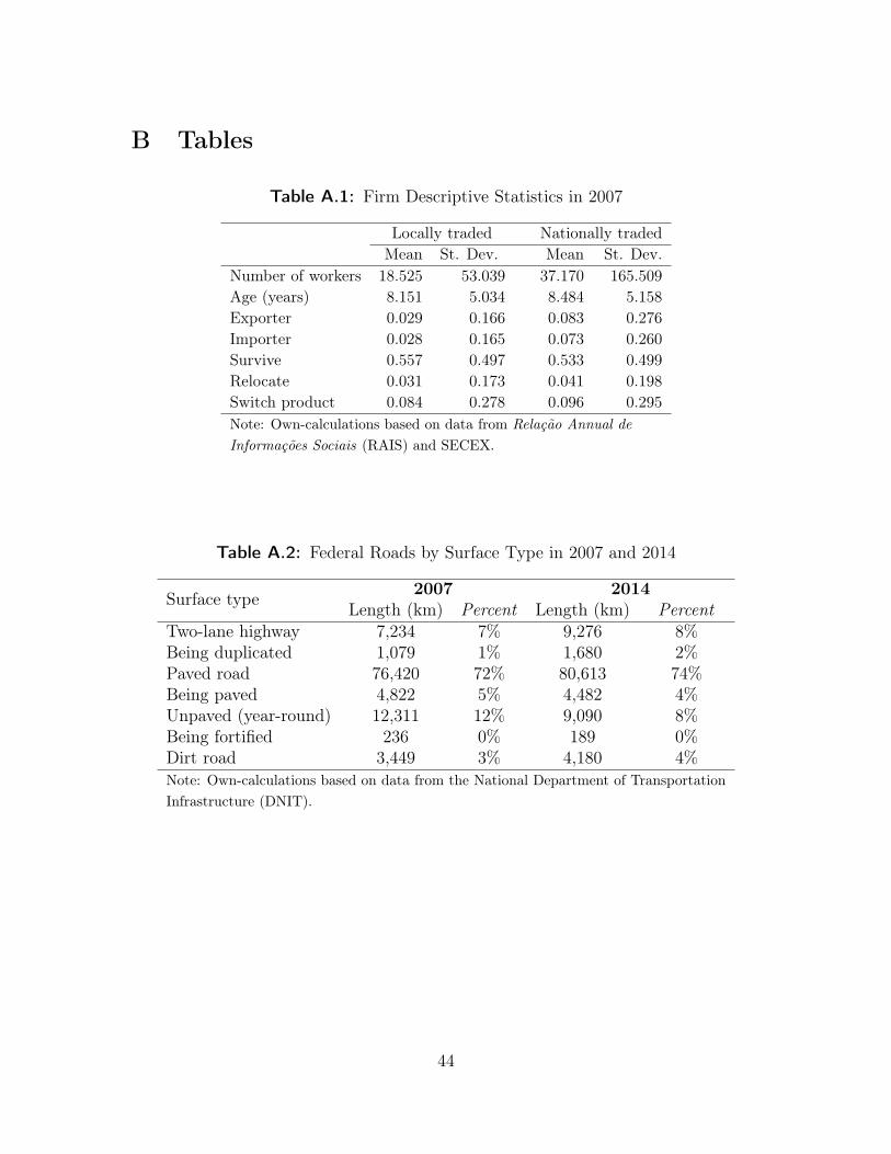
B Tables

Table A.1: Firm Descriptive Statistics in 2007

Locally traded Nationally tradedMean St. Dev. Mean St. Dev.

Number of workers 18.525 53.039 37.170 165.509Age (years) 8.151 5.034 8.484 5.158Exporter 0.029 0.166 0.083 0.276Importer 0.028 0.165 0.073 0.260Survive 0.557 0.497 0.533 0.499Relocate 0.031 0.173 0.041 0.198Switch product 0.084 0.278 0.096 0.295Note: Own-calculations based on data from Relação Annual deInformações Sociais (RAIS) and SECEX.

Table A.2: Federal Roads by Surface Type in 2007 and 2014

Surface type 2007 2014Length (km) Percent Length (km) Percent

Two-lane highway 7,234 7% 9,276 8%Being duplicated 1,079 1% 1,680 2%Paved road 76,420 72% 80,613 74%Being paved 4,822 5% 4,482 4%Unpaved (year-round) 12,311 12% 9,090 8%Being fortified 236 0% 189 0%Dirt road 3,449 3% 4,180 4%Note: Own-calculations based on data from the National Department of TransportationInfrastructure (DNIT).

44

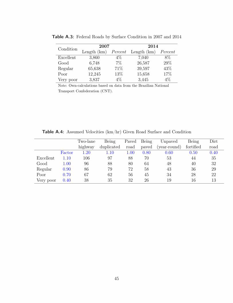
Table A.3: Federal Roads by Surface Condition in 2007 and 2014

Condition 2007 2014Length (km) Percent Length (km) Percent

Excellent 3,860 4% 7,040 8%Good 6,748 7% 26,587 29%Regular 65,638 71% 39,597 43%Poor 12,245 13% 15,658 17%Very poor 3,837 4% 3,445 4%Note: Own-calculations based on data from the Brazilian NationalTransport Confederation (CNT).

Table A.4: Assumed Velocities (km/hr) Given Road Surface and Condition

Two-lane Being Paved Being Unpaved Being Dirthighway duplicated road paved (year-round) fortified road

Factor 1.20 1.10 1.00 0.80 0.60 0.50 0.40Excellent 1.10 106 97 88 70 53 44 35Good 1.00 96 88 80 64 48 40 32Regular 0.90 86 79 72 58 43 36 29Poor 0.70 67 62 56 45 34 28 22Very poor 0.40 38 35 32 26 19 16 13

45

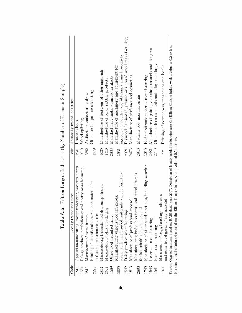
Tab

leA.5

:FifteenLa

rgestIndu

stries

(byNum

berof

Firmsin

Sample)

Cod

eLo

cally

trad

edindu

stries

Cod

eNationa

llytrad

edindu

stries

1812

App

arel

man

ufacturing

,exceptun

derw

ear,

sweaters,s

hirts

1931

Leathershoes

1581

Bakeryprod

ucts,c

onfectione

ryan

dpa

stry

man

ufacturing

2010

Woo

dsplitting

2812

Man

ufacture

ofmetal

fram

es28

92Artifa

ctsman

ufacturing

draw

n

2222

Printingof

educ

ationa

lmaterial,an

dmaterialfor

1779

Other

textile

prod

ucts

knitting

indu

strial

orcommercial

uses

2842

Man

ufacturing

locksm

itharticles,e

xcep

tfram

es19

39Man

ufacture

offootwearof

othermaterials

2522

Man

ufacture

ofplasticpa

ckag

ing

2519

Man

ufacture

ofotherrubb

erprod

ucts

1589

Other

food

man

ufacturing

2833

Man

ufacturing

metal

stam

pedartifacts

2029

Man

ufacturing

variou

swoo

dengo

ods,

2931

Man

ufacture

ofmachinery

andequipm

entfor

straw,c

orkan

dbraidedmaterials,e

xceptfurniture

agriculture,

poultryan

dob

tainingan

imal

prod

ucts

1542

Dairy

prod

uctman

ufacturing

2021

Plywoo

d,laminated,p

ressed

orsintered

woo

dman

ufacturing

1813

Man

ufacture

ofprofession

alap

parel

2473

Man

ufacture

ofpe

rfum

esan

dcosm

etics

2893

Man

ufacturing

body

shop

item

san

dmetal

articles

2940

Machine

tool

man

ufacturing

forho

useholdusean

dpe

rson

al17

49Man

ufacture

ofothertextile

articles,including

weaving

3210

Basic

electron

icmaterialm

anufacturing

1543

Icecream

man

ufacturing

2481

Man

ufacture

ofpa

ints,v

arnishes,e

namelsan

dlacquers

1584

Pasta

man

ufacturing

2749

Other

non-ferrou

smetalsan

dalloymetallurgy

1921

Man

ufacture

ofba

gs,h

andb

ags,

suitcases

2221

Printingof

newspap

ers,

mag

azines

andbo

oks

andothe

rtravel

good

sof

anymaterial

Source:Owncalculations

basedon

RAIS

data,y

ear20

07.Definition

oflocally

trad

edindu

stries

uses

theEllison-Glaeser

index,

withavalueof

0.2or

less.

Nationa

llytrad

edindu

stries

basedon

theEllison-Glaeser

index,

withavalueof

0.5or

more.

46

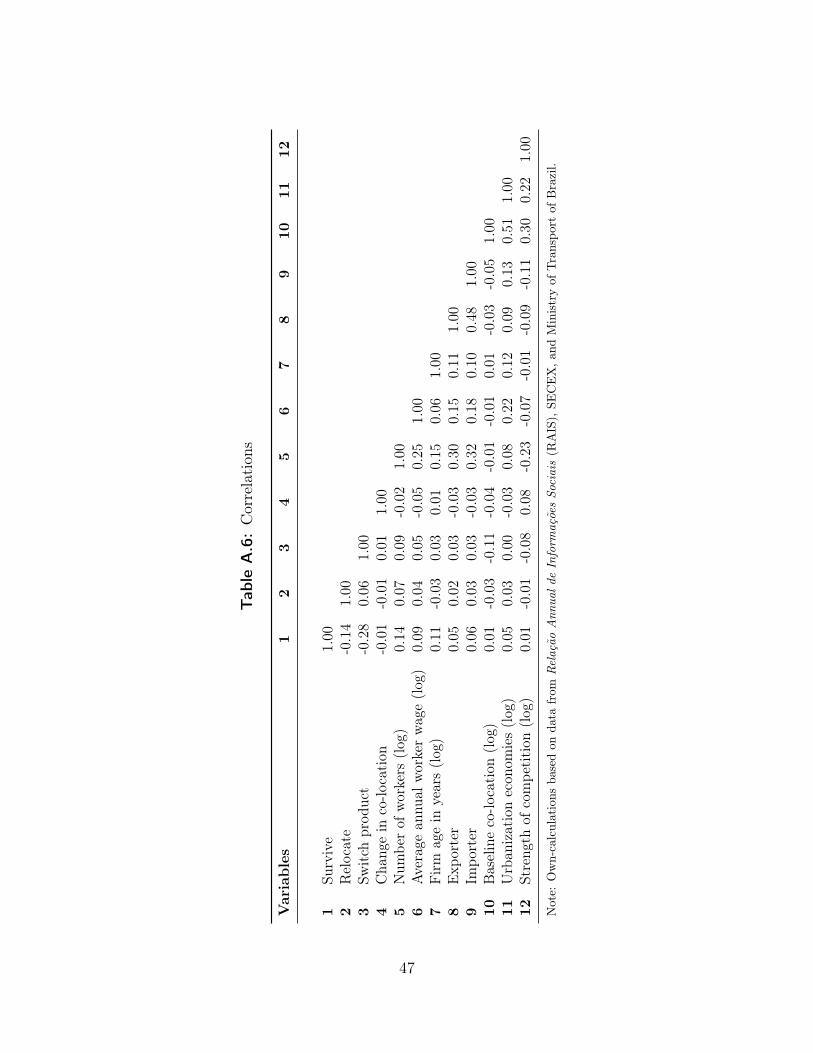
Tab

leA.6

:Correlation

s

Var

iable

s1

23

45

67

89

1011

12

1Su

rvive

1.00

2Relocate

-0.14

1.00

3Sw

itch

prod

uct

-0.28

0.06

1.00

4Cha

ngein

co-lo

cation

-0.01

-0.01

0.01

1.00

5Num

berof

workers

(log)

0.14

0.07

0.09

-0.02

1.00

6Av

erag

ean

nual

workerwag

e(log

)0.09

0.04

0.05

-0.05

0.25

1.00

7Firm

agein

years(log

)0.11

-0.03

0.03

0.01

0.15

0.06

1.00

8Exp

orter

0.05

0.02

0.03

-0.03

0.30

0.15

0.11

1.00

9Im

porter

0.06

0.03

0.03

-0.03

0.32

0.18

0.10

0.48

1.00

10Baselineco-lo

cation

(log

)0.01

-0.03

-0.11

-0.04

-0.01

-0.01

0.01

-0.03

-0.05

1.00

11Urban

izationecon

omies(log

)0.05

0.03

0.00

-0.03

0.08

0.22

0.12

0.09

0.13

0.51

1.00

12Streng

thof

compe

tition

(log

)0.01

-0.01

-0.08

0.08

-0.23

-0.07

-0.01

-0.09

-0.11

0.30

0.22

1.00

Note:

Own-calculations

basedon

data

from

Rel

ação

Ann

uald

eIn

form

açõe

sSo

ciai

s(R

AIS),SE

CEX,a

ndMinistryof

Transpo

rtof

Brazil.

47

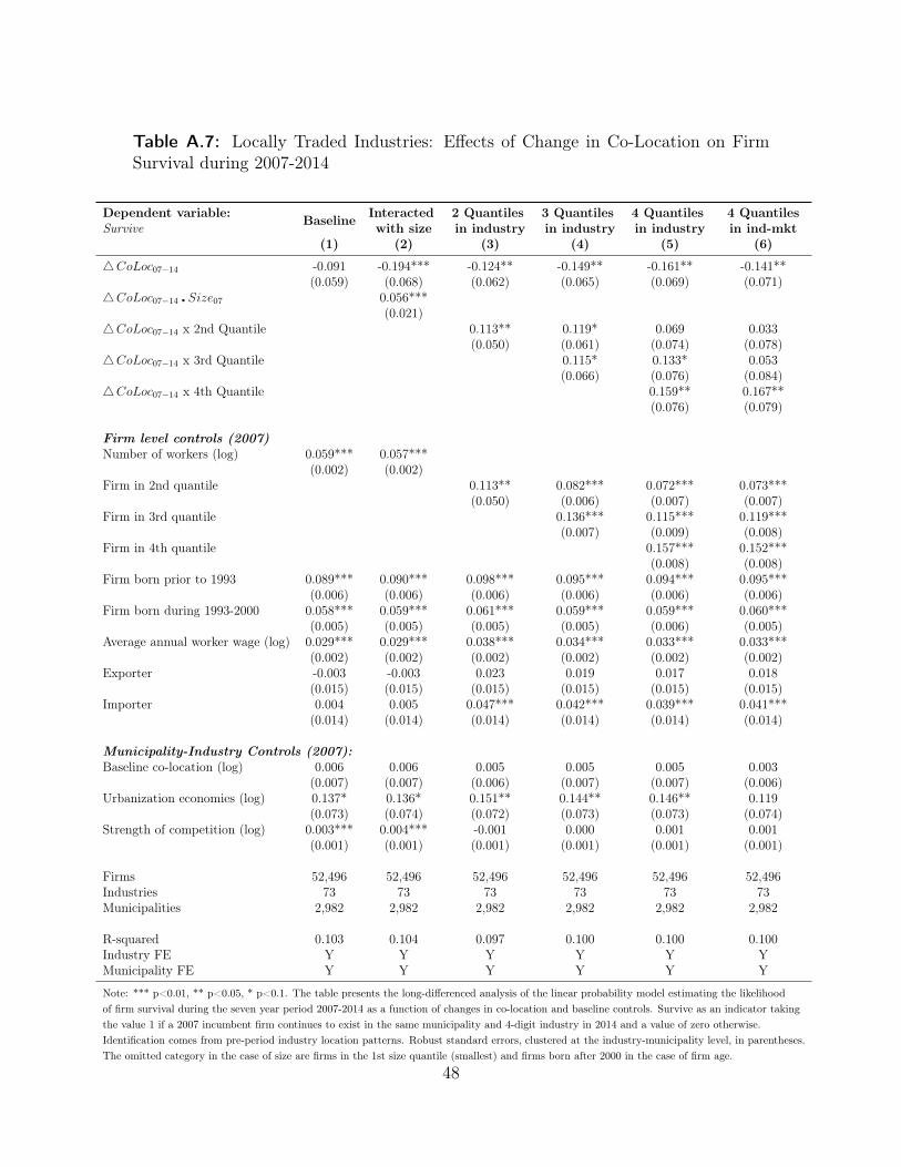
Table A.7: Locally Traded Industries: Effects of Change in Co-Location on FirmSurvival during 2007-2014

Dependent variable: Baseline Interacted 2 Quantiles 3 Quantiles 4 Quantiles 4 QuantilesSurvive with size in industry in industry in industry in ind-mkt

(1) (2) (3) (4) (5) (6)

4CoLoc07−14 -0.091 -0.194*** -0.124** -0.149** -0.161** -0.141**(0.059) (0.068) (0.062) (0.065) (0.069) (0.071)

4CoLoc07−14 � Size07 0.056***(0.021)

4CoLoc07−14 x 2nd Quantile 0.113** 0.119* 0.069 0.033(0.050) (0.061) (0.074) (0.078)

4CoLoc07−14 x 3rd Quantile 0.115* 0.133* 0.053(0.066) (0.076) (0.084)

4CoLoc07−14 x 4th Quantile 0.159** 0.167**(0.076) (0.079)

Firm level controls (2007)Number of workers (log) 0.059*** 0.057***

(0.002) (0.002)Firm in 2nd quantile 0.113** 0.082*** 0.072*** 0.073***

(0.050) (0.006) (0.007) (0.007)Firm in 3rd quantile 0.136*** 0.115*** 0.119***

(0.007) (0.009) (0.008)Firm in 4th quantile 0.157*** 0.152***

(0.008) (0.008)Firm born prior to 1993 0.089*** 0.090*** 0.098*** 0.095*** 0.094*** 0.095***

(0.006) (0.006) (0.006) (0.006) (0.006) (0.006)Firm born during 1993-2000 0.058*** 0.059*** 0.061*** 0.059*** 0.059*** 0.060***

(0.005) (0.005) (0.005) (0.005) (0.006) (0.005)Average annual worker wage (log) 0.029*** 0.029*** 0.038*** 0.034*** 0.033*** 0.033***

(0.002) (0.002) (0.002) (0.002) (0.002) (0.002)Exporter -0.003 -0.003 0.023 0.019 0.017 0.018

(0.015) (0.015) (0.015) (0.015) (0.015) (0.015)Importer 0.004 0.005 0.047*** 0.042*** 0.039*** 0.041***

(0.014) (0.014) (0.014) (0.014) (0.014) (0.014)

Municipality-Industry Controls (2007):Baseline co-location (log) 0.006 0.006 0.005 0.005 0.005 0.003

(0.007) (0.007) (0.006) (0.007) (0.007) (0.006)Urbanization economies (log) 0.137* 0.136* 0.151** 0.144** 0.146** 0.119

(0.073) (0.074) (0.072) (0.073) (0.073) (0.074)Strength of competition (log) 0.003*** 0.004*** -0.001 0.000 0.001 0.001

(0.001) (0.001) (0.001) (0.001) (0.001) (0.001)

Firms 52,496 52,496 52,496 52,496 52,496 52,496Industries 73 73 73 73 73 73Municipalities 2,982 2,982 2,982 2,982 2,982 2,982

R-squared 0.103 0.104 0.097 0.100 0.100 0.100Industry FE Y Y Y Y Y YMunicipality FE Y Y Y Y Y Y

Note: *** p<0.01, ** p<0.05, * p<0.1. The table presents the long-differenced analysis of the linear probability model estimating the likelihoodof firm survival during the seven year period 2007-2014 as a function of changes in co-location and baseline controls. Survive as an indicator takingthe value 1 if a 2007 incumbent firm continues to exist in the same municipality and 4-digit industry in 2014 and a value of zero otherwise.Identification comes from pre-period industry location patterns. Robust standard errors, clustered at the industry-municipality level, in parentheses.The omitted category in the case of size are firms in the 1st size quantile (smallest) and firms born after 2000 in the case of firm age.

48

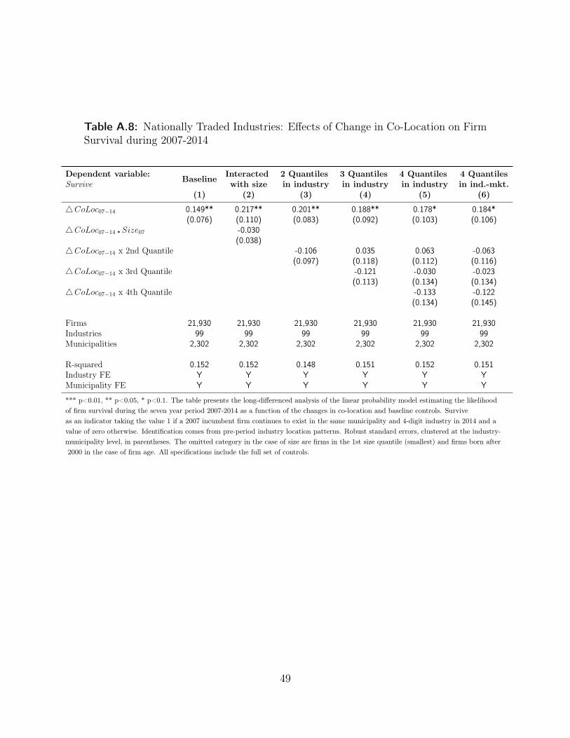
Table A.8: Nationally Traded Industries: Effects of Change in Co-Location on FirmSurvival during 2007-2014

Dependent variable: Baseline Interacted 2 Quantiles 3 Quantiles 4 Quantiles 4 QuantilesSurvive with size in industry in industry in industry in ind.-mkt.

(1) (2) (3) (4) (5) (6)

4CoLoc07−14 0.149** 0.217** 0.201** 0.188** 0.178* 0.184*(0.076) (0.110) (0.083) (0.092) (0.103) (0.106)

4CoLoc07−14 � Size07 -0.030(0.038)

4CoLoc07−14 x 2nd Quantile -0.106 0.035 0.063 -0.063(0.097) (0.118) (0.112) (0.116)

4CoLoc07−14 x 3rd Quantile -0.121 -0.030 -0.023(0.113) (0.134) (0.134)

4CoLoc07−14 x 4th Quantile -0.133 -0.122(0.134) (0.145)

Firms 21,930 21,930 21,930 21,930 21,930 21,930Industries 99 99 99 99 99 99Municipalities 2,302 2,302 2,302 2,302 2,302 2,302

R-squared 0.152 0.152 0.148 0.151 0.152 0.151Industry FE Y Y Y Y Y YMunicipality FE Y Y Y Y Y Y

*** p<0.01, ** p<0.05, * p<0.1. The table presents the long-differenced analysis of the linear probability model estimating the likelihoodof firm survival during the seven year period 2007-2014 as a function of the changes in co-location and baseline controls. Surviveas an indicator taking the value 1 if a 2007 incumbent firm continues to exist in the same municipality and 4-digit industry in 2014 and avalue of zero otherwise. Identification comes from pre-period industry location patterns. Robust standard errors, clustered at the industry-municipality level, in parentheses. The omitted category in the case of size are firms in the 1st size quantile (smallest) and firms born after2000 in the case of firm age. All specifications include the full set of controls.

49

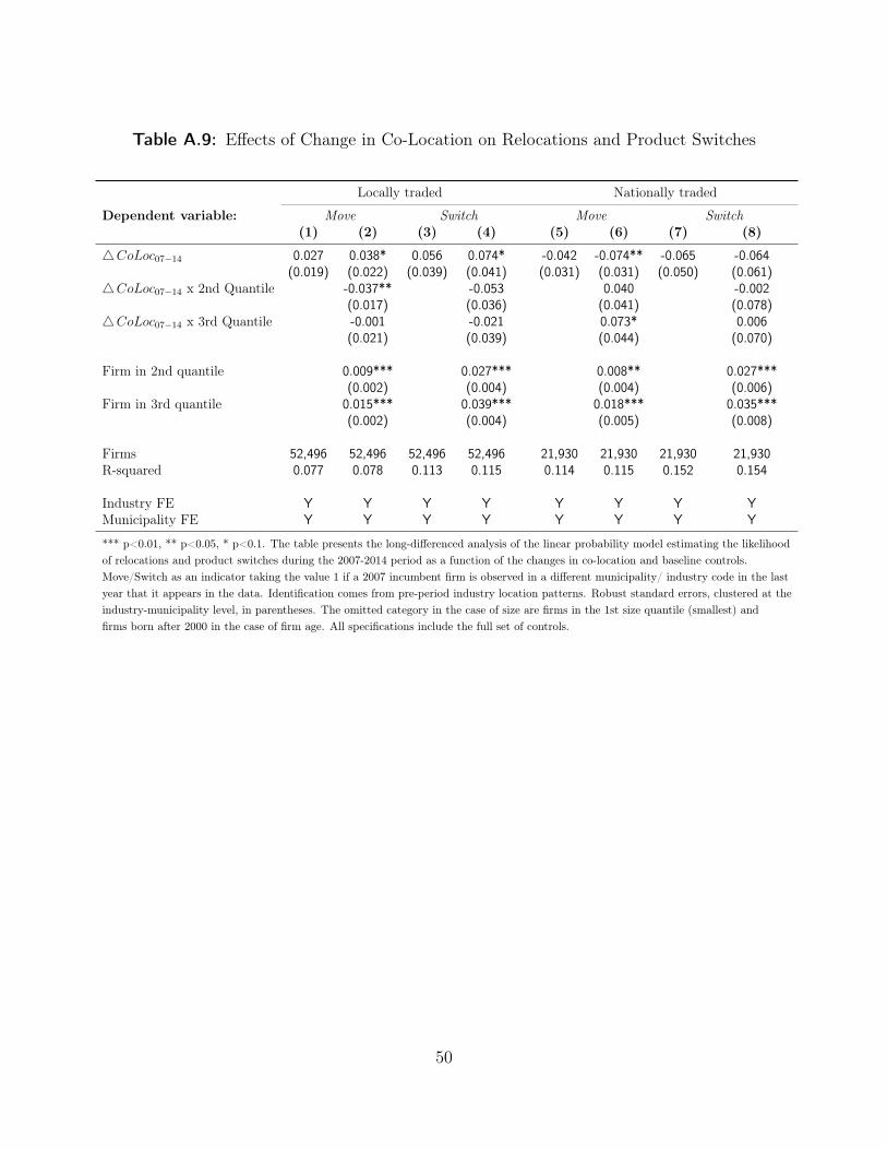
Table A.9: Effects of Change in Co-Location on Relocations and Product Switches

Locally traded Nationally traded

Dependent variable: Move Switch Move Switch(1) (2) (3) (4) (5) (6) (7) (8)

4CoLoc07−14 0.027 0.038* 0.056 0.074* -0.042 -0.074** -0.065 -0.064(0.019) (0.022) (0.039) (0.041) (0.031) (0.031) (0.050) (0.061)

4CoLoc07−14 x 2nd Quantile -0.037** -0.053 0.040 -0.002(0.017) (0.036) (0.041) (0.078)

4CoLoc07−14 x 3rd Quantile -0.001 -0.021 0.073* 0.006(0.021) (0.039) (0.044) (0.070)

Firm in 2nd quantile 0.009*** 0.027*** 0.008** 0.027***(0.002) (0.004) (0.004) (0.006)

Firm in 3rd quantile 0.015*** 0.039*** 0.018*** 0.035***(0.002) (0.004) (0.005) (0.008)

Firms 52,496 52,496 52,496 52,496 21,930 21,930 21,930 21,930R-squared 0.077 0.078 0.113 0.115 0.114 0.115 0.152 0.154

Industry FE Y Y Y Y Y Y Y YMunicipality FE Y Y Y Y Y Y Y Y

*** p<0.01, ** p<0.05, * p<0.1. The table presents the long-differenced analysis of the linear probability model estimating the likelihoodof relocations and product switches during the 2007-2014 period as a function of the changes in co-location and baseline controls.Move/Switch as an indicator taking the value 1 if a 2007 incumbent firm is observed in a different municipality/ industry code in the lastyear that it appears in the data. Identification comes from pre-period industry location patterns. Robust standard errors, clustered at theindustry-municipality level, in parentheses. The omitted category in the case of size are firms in the 1st size quantile (smallest) andfirms born after 2000 in the case of firm age. All specifications include the full set of controls.

50