When the Threat is Stronger than the Execution: Trade...
36
When the Threat is Stronger than the Execution: Trade Liberalization and Welfare under Oligopoly Dermot Leahy Maynooth University J. Peter Neary Oxford, CEPR and CESifo ESEM 2016, Geneva August 24, 2016 Leahy and Neary (Maynooth and Oxford) Trade Liberalization under Oligopoly ESEM: August 24, 2016 1 / 34
-
Upload
nguyendung -
Category
Documents
-
view
219 -
download
1
Transcript of When the Threat is Stronger than the Execution: Trade...

When the Threat is Stronger than the Execution:Trade Liberalization and Welfare under Oligopoly
Dermot Leahy
Maynooth University
J. Peter Neary
Oxford, CEPR and CESifo
ESEM 2016, GenevaAugust 24, 2016
Leahy and Neary (Maynooth and Oxford) Trade Liberalization under Oligopoly ESEM: August 24, 2016 1 / 34

Introduction
Aron Nimzowitsch
Aron Nimzowitsch, 1886–1935
“The threat is stronger than the execution”
Leahy and Neary (Maynooth and Oxford) Trade Liberalization under Oligopoly ESEM: August 24, 2016 2 / 34

Introduction
Introduction
Trade policy: Gains from trade liberalization
The magnitude of the gains is still a central issue in international trade.Recent work sheds light on the quantitative extent of gains underperfect competition and monopolistic competition with heterogeneousfirms.Less work has been done on trade liberalization under oligopoly.
Despite growing evidence that trade is dominated by large firms.Mayer and Ottaviano (2008), Freund and Pierola (2015)
IO: Oligopoly with cost asymmetries
Who gains and who loses as best-practice technology disseminates?
Leahy and Neary (Maynooth and Oxford) Trade Liberalization under Oligopoly ESEM: August 24, 2016 3 / 34

Introduction
Our Contribution
We compare trade liberalization under Cournot and Bertrandoligopoly in a unified framework with product differentiation.
Common perception that the results of oligopoly trade models arehighly sensitive to the mode of competition.We show that many of the predictions are qualitatively robust towhether firms compete on quantity or price.But: There are important differences between the two cases.
Details:
We use duopoly with linear demands to obtain explicit solutions.Then extend the analysis to oligopoly and more general functionalforms: results are qualitatively robust.
Take-Home:
Firms compete more aggressively under Bertrand than under Cournot.This affects outcomes even when there is no trade under Bertrand.
Leahy and Neary (Maynooth and Oxford) Trade Liberalization under Oligopoly ESEM: August 24, 2016 4 / 34

Introduction
Background Literature
Quantity versus price competition:
Singh and Vives (1984), Vives (1985)
Oligopoly with cost asymmetries:
Lahiri and Ono (1988), Neary (1994)
Welfare effects of trade liberalization under oligopoly:
Use the reciprocal-markets model first developed by Brander (1981)and Brander and Krugman (1983).
Extended by Bernhofen (2001) - Product differentiation.
Clarke and Collie (2003) - Bertrand.
Brander and Spencer (2015), Collie and Le (2015).
For a survey see: Leahy and Neary (2011).
A simultaneous-move game, not about entry deterrence:
Spence (1977), Dixit (1980), Fudenberg-Tirole (1985), Neary (2002)
Leahy and Neary (Maynooth and Oxford) Trade Liberalization under Oligopoly ESEM: August 24, 2016 5 / 34

Introduction
Outline
1 The Model
2 Equilibria with Trade
3 The Nimzowitsch Region
4 General Demands
5 Conclusion
Leahy and Neary (Maynooth and Oxford) Trade Liberalization under Oligopoly ESEM: August 24, 2016 6 / 34

The Model
Outline
1 The ModelUtility and DemandTechnology and Firm Behavior
2 Equilibria with Trade
3 The Nimzowitsch Region
4 General Demands
5 Conclusion
Leahy and Neary (Maynooth and Oxford) Trade Liberalization under Oligopoly ESEM: August 24, 2016 7 / 34

The Model Utility and Demand
The Model
A symmetric two-country model, with segmented markets.
A home and foreign firm compete in both home and foreign markets.
Demand:
A representative consumer in the home country with quasi-linear utility:
U = z0 + u(x, y)
We first assume a quadratic sub-utility function:
u(x, y) = a(x + y)− b2(x2 + 2exy + y2)
Maximization of utility subject to the budget constraint yields linearinverse demand functions:
p = a− b(x + ey) and p∗ = a− b(y + ex)
Leahy and Neary (Maynooth and Oxford) Trade Liberalization under Oligopoly ESEM: August 24, 2016 8 / 34

The Model Technology and Firm Behavior
Technology and Firm Behavior
Costs:
Marginal costs are constant and we ignore fixed costs.
Profits: Home market profits of the home and foreign firm are:π = (p− c)xπ∗ = (p∗ − c− t)y
Symmetric multilateral trade liberalization under:1 Quantity/Cournot competition2 Price/Bertrand competition
The symmetric case, where the home and foreign firms facesymmetric demands, the same production cost functions, and thesame trade cost.
Leahy and Neary (Maynooth and Oxford) Trade Liberalization under Oligopoly ESEM: August 24, 2016 9 / 34

Equilibria with Trade
Outline
1 The Model
2 Equilibria with TradeQuantity CompetitionPrice CompetitionBertrand vs. Cournot
3 The Nimzowitsch Region
4 General Demands
5 Conclusion
Leahy and Neary (Maynooth and Oxford) Trade Liberalization under Oligopoly ESEM: August 24, 2016 10 / 34

Equilibria with Trade Quantity Competition
Quantity Competition: Outputs and Profits
Home market outputs:
Free trade: xCF = yCF = Ab(2+e) A ≡ a− c
Prohibitive trade cost: y = 0 → tC = 2−e2 A
⇒ xC = xCF(
1 +e2
ttC
)and yC = yCF
(1− t
tC
)
Profits of home firm:
Due to symmetry, home exports x∗ equal home imports y, → homefirm’s profits on its exports are π∗ = (p∗ − c− t)x∗ = (p∗ − c− t)y.
Effect of a multilateral change in trade costs on total profits:
d (π + π∗)dt
=2(ex− 2x∗)
4− e2
{< 0 when t = 0 (so x = x∗)> 0 when t = tC (so x∗ = 0)
So: Profits are U-shaped in t.
Leahy and Neary (Maynooth and Oxford) Trade Liberalization under Oligopoly ESEM: August 24, 2016 11 / 34

Equilibria with Trade Quantity Competition
Quantity Competition: Outputs and Profits
Home market outputs:
Free trade: xCF = yCF = Ab(2+e) A ≡ a− c
Prohibitive trade cost: y = 0 → tC = 2−e2 A
⇒ xC = xCF(
1 +e2
ttC
)and yC = yCF
(1− t
tC
)Profits of home firm:
Due to symmetry, home exports x∗ equal home imports y, → homefirm’s profits on its exports are π∗ = (p∗ − c− t)x∗ = (p∗ − c− t)y.
Effect of a multilateral change in trade costs on total profits:
d (π + π∗)dt
=2(ex− 2x∗)
4− e2
{< 0 when t = 0 (so x = x∗)> 0 when t = tC (so x∗ = 0)
So: Profits are U-shaped in t.
Leahy and Neary (Maynooth and Oxford) Trade Liberalization under Oligopoly ESEM: August 24, 2016 11 / 34

Equilibria with Trade Quantity Competition
Cournot Profits
Trade is locally bad for profits, in the neighbourhood of autarky.
Must it be globally bad? Anderson, Donsimoni, and Gabszewicz(1989) showed that it is when goods are perfect substitutes.
However, trade liberalization is less bad for firms when e is lower.
0.0
0.1
0.2
0.3
0.4
0.5
0.6
0.7
0.8
0.9
1.0
0.0 0.2 0.4 0.6 0.8 1.0
t
e
t^C
t‐min
t‐eq
Loci of t and e that yield Autarky, Minimum Profits, and Autarky Profits
Leahy and Neary (Maynooth and Oxford) Trade Liberalization under Oligopoly ESEM: August 24, 2016 12 / 34

Equilibria with Trade Quantity Competition
Welfare under Cournot
Consumer surplus rises monotonically as trade costs fall. (Prices ofboth goods fall)Hence, the range of t where welfare is lower than autarky is smallerthan that where profits are lower.Welfare is also U-shaped in t. It falls below the autarky level betweenthe upper and lower loci reaching a minimum along the middle locus.
0.0
0.1
0.2
0.3
0.4
0.5
0.6
0.7
0.8
0.9
1.0
0.0 0.2 0.4 0.6 0.8 1.0
t
e
t^C
t‐min
t‐eq
Loci of t and e that yield Autarky, Minimum Profits, and Autarky Welfare
Leahy and Neary (Maynooth and Oxford) Trade Liberalization under Oligopoly ESEM: August 24, 2016 13 / 34
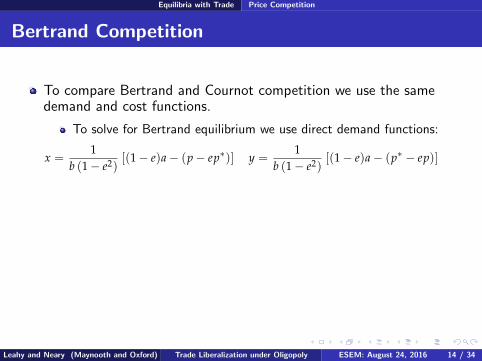
Equilibria with Trade Price Competition
Bertrand Competition
To compare Bertrand and Cournot competition we use the samedemand and cost functions.
To solve for Bertrand equilibrium we use direct demand functions:
x =1
b (1− e2)[(1− e)a− (p− ep∗)] y =
1b (1− e2)
[(1− e)a− (p∗ − ep)]
Home market outputs:
Free trade: xBF = yBF = Ab(2+e−e2)
Prohibitive trade cost: y = 0 → tB = (1−e)(2+e)2−e2 A
⇒ xB = xBF(
1 +e
2− e2t
tB
)and yB = yBF
(1− t
tB
)
Leahy and Neary (Maynooth and Oxford) Trade Liberalization under Oligopoly ESEM: August 24, 2016 14 / 34

Equilibria with Trade Bertrand vs. Cournot
Bertrand vs. Cournot
Straightforward to show that: tB < tC
Profits and welfare also behave similarly to quantity competition fortrade costs between zero and tB.As shown by Vives (1985): price competition is more competitive thanquantity competition in symmetric equilibrium: price competitionleads to lower prices and higher outputs and thus higher welfare.
With linear demands, even with asymmetric firms, price competitionalways leads to higher welfare for t ≤ tB:
WB −WC =1b
e2
(1 + e) (4− e2)2
{(4− e2 − 2e
)A(A− t) +
(4 + e2)
2(1− e)t2
}
Leahy and Neary (Maynooth and Oxford) Trade Liberalization under Oligopoly ESEM: August 24, 2016 15 / 34

Equilibria with Trade Bertrand vs. Cournot
Bertrand vs. Cournot WelfareQualitatively similar as trade costs fall, but also differences:
W
t
WB-WA
WC-WA
Effects of Trade Liberalization on Welfare in Cournot and Bertrand Competition
Leahy and Neary (Maynooth and Oxford) Trade Liberalization under Oligopoly ESEM: August 24, 2016 16 / 34

The Nimzowitsch Region
Outline
1 The Model
2 Equilibria with Trade
3 The Nimzowitsch RegionThe Nimzowitsch Region: Home Best ResponseWelfare in the Nimzowitsch Region
4 General Demands
5 Conclusion
Leahy and Neary (Maynooth and Oxford) Trade Liberalization under Oligopoly ESEM: August 24, 2016 17 / 34

The Nimzowitsch Region
The Nimzowitsch Region
A region of trade costs too high for trade in Bertrand, but low enoughto allow the threat of trade.
Between tB and tC no trade occurs under price competition.
Yet (with linear demands) the pro-competitive threat of trade raiseswelfare above the Cournot level.The threat of trade raises welfare more than actual trade underCournot.We call the region of parameter space in which this outcome holds the“Nimzowitsch Region”.
Leahy and Neary (Maynooth and Oxford) Trade Liberalization under Oligopoly ESEM: August 24, 2016 18 / 34

The Nimzowitsch Region
Trade under Price and Output Competition
t
e
N
M
CB
Regions of Trade
B: yB > yC ; C: yC > yB > 0; N: Nimzowitsch Region; A: Autarky
Leahy and Neary (Maynooth and Oxford) Trade Liberalization under Oligopoly ESEM: August 24, 2016 19 / 34

The Nimzowitsch Region The Nimzowitsch Region: Home Best Response
The Nimzowitsch Region
At tB there is no trade under Bertrand but the domestic firm’s price isbelow the monopoly level.
The home firm does not raise its price, since its rival would then makepositive sales lowering the home firm’s domestic profits.When t reaches tC the home firm can act as an unconstrainedmonopolist.When tB ≤ t ≤ tC, the home firm chooses a price at which the foreignfirm is just unable to produce.Domestic output is: x = A−t
be which falls in t.Since x falls in t in the region tB ≤ t ≤ tC and y = 0, welfare is fallingin t in that region.Hence under price competition, unlike under quantity competition,trade liberalization starting from autarky initially raises welfare
Leahy and Neary (Maynooth and Oxford) Trade Liberalization under Oligopoly ESEM: August 24, 2016 20 / 34

The Nimzowitsch Region The Nimzowitsch Region: Home Best Response
Bertrand vs. Cournot Outputs
0.0
0.1
0.2
0.3
0.4
0.5
0.6
0.7
0.8
0.9
1.0
0.0 0.2 0.4 0.6
xC
yC
xB
yB
XC
XB
Leahy and Neary (Maynooth and Oxford) Trade Liberalization under Oligopoly ESEM: August 24, 2016 21 / 34

The Nimzowitsch Region Welfare in the Nimzowitsch Region
Welfare in the Nimzowitsch Region
Welfare under price and output competition:
W
t
WB-WA
WC-WA
Nimzovitsch Region
Leahy and Neary (Maynooth and Oxford) Trade Liberalization under Oligopoly ESEM: August 24, 2016 22 / 34

The Nimzowitsch Region Welfare in the Nimzowitsch Region
Strategic Interactions in the Nimzowitsch Region
*p
p
)(~ pp*
);(~ tpB*
tc );( tpB*
(a) ForeignBest-Response Function
*p
p
)(~ *pp)( *pB )(~
*pB
Btc ˆ
Ctc ˆ
Mp
(b) HomeBest-Response Function
*p
p
)(~*pB
);(~ tpB*
(c) Equilibrium in theNimzowitsch Region
Leahy and Neary (Maynooth and Oxford) Trade Liberalization under Oligopoly ESEM: August 24, 2016 23 / 34

The Nimzowitsch Region Welfare in the Nimzowitsch Region
Minimum versus Maximum Import Constraints
Contrast:1 Here: Imports are non-negative: y ≥ 02 Krishna (JIE 1989): Import quota: y ≤ y
Both extend classic results to product differentiation:1 Low-cost firm prices at marginal cost of high-cost
2 No pure-strategy equilibrium with capacity constraints [Edgeworth]
In both, home firm’s best response is a choice between two options:When import constraint binds, a high price yields monopoly profits
When it does not, a low price leads to a standard Bertrand equilibrium
For both options, profits given p∗ are concave in p1 Here: Maximum profits is the lower envelope
Which is itself concave
2 Krishna: Maximum profits is the upper envelopeSo: no equilibrium in pure strategies
Leahy and Neary (Maynooth and Oxford) Trade Liberalization under Oligopoly ESEM: August 24, 2016 24 / 34

The Nimzowitsch Region Welfare in the Nimzowitsch Region
The Nimzowitsch Region: The Home Firm
c+tBc+t
c+tC
pM p
y=0p
p*
y>0M B
y=0
Price Competition: The Home Firm’s Perspective
Leahy and Neary (Maynooth and Oxford) Trade Liberalization under Oligopoly ESEM: August 24, 2016 25 / 34

General Demands
Outline
1 The Model
2 Equilibria with Trade
3 The Nimzowitsch Region
4 General DemandsFree Trade and AutarkyThe Volume of TradeWelfare
5 Conclusion
Leahy and Neary (Maynooth and Oxford) Trade Liberalization under Oligopoly ESEM: August 24, 2016 26 / 34

General Demands
General Demands
Do these results continue to hold with general demands?
p(x, y) for the home good and p∗(y, x) for the foreign?
We assume that the demand functions are twice differentiable andstrictly decreasing in own price, px < 0 and p∗y < 0.
We also assume that p∗(0, x) < ∞ so that foreign demand has a chokeprice and a prohibitive trade cost exists.
We assume that the demand system can be inverted to get:
x(p, p∗) for the home good and y(p∗, p) for the foreign.
Leahy and Neary (Maynooth and Oxford) Trade Liberalization under Oligopoly ESEM: August 24, 2016 27 / 34

General Demands Free Trade and Autarky
Free Trade and Autarky
We impose a few additional mild restrictions such as:
Marginal revenue is always downward-slopingHome marginal revenue falls in a symmetric equilibrium following anequal increase in the outputs of both goodsWe do not restrict quantities to be strategic substitutes under Cournotnor prices to be strategic complements under Bertrand
Given these we are able to show:
1 At t = 0, the volume of trade is higher under Bertrand than Cournot.Prices at t = 0 are lower under Bertrand than Cournot. (This result isimplicit in Vives (1985) who did not look at trade)
2 tB < tC
Leahy and Neary (Maynooth and Oxford) Trade Liberalization under Oligopoly ESEM: August 24, 2016 28 / 34

General Demands The Volume of Trade
The Volume of Trade
The volume of trade under price and output competition:
Here a single intersection but in general there could be many.
Showing that xB > xC
c
r
r(xB)+β(xB)=cr(xC)=c
r(xC)
r,c
x
r(xB)
xC xB
ttCtB
yC(0)
yB(0)
Figure 1
4
Volume of Trade under Quantity and Price Competition
Leahy and Neary (Maynooth and Oxford) Trade Liberalization under Oligopoly ESEM: August 24, 2016 29 / 34

General Demands Welfare
Welfare
Welfare change dW = dχ + dΠ can be written as:
dW = (p− c)dx + (p∗ − c− t)dy− ydt
1 At t = 0 this is dWdt = (p− c)( dx
dt +dydt )− y < 0 under both quantity
and price competition. So at free trade an increase in trade costs isbad. This generalises the result under linear demands.
2 At tC under Cournot we have dx/dt > 0 (if outputs are strategicsubtitutes) so dW
dt = (p− c) dxdt > 0. A small fall in trade costs is bad.
Unlike the linear demand case these results can only be stated atparticular points.
Leahy and Neary (Maynooth and Oxford) Trade Liberalization under Oligopoly ESEM: August 24, 2016 30 / 34

General Demands Welfare
Welfare in the Nimzowitsch Region
The Nimzowitsch Region: {tB, tC}Consider Bertrand competition only:
Equilibrium has y = 0.Hence p∗(0, x)− c− t = 0, implying that x must decrease in t
dx/dt = 1/p∗x(0, x) < 0So a decrease in t between tB and tC raises welfare.At tB a small fall in trade costs under Bertrand lowers welfare (ifdx/dt > 0 ).
This allows us to sign the following derivatives:
dWB
dt
∣∣∣∣tC ,−
< 0dWB
dt
∣∣∣∣tB ,−
> 0dWB
dt
∣∣∣∣tB ,+
< 0
Leahy and Neary (Maynooth and Oxford) Trade Liberalization under Oligopoly ESEM: August 24, 2016 31 / 34

General Demands Welfare
Welfare with General Demands: Summary
W
t
WB-WA
WC-WA(1)
(2)
(3) (4)
(5)
(6)
With general demands, we can only sign the end-pointsBut the results confirm qualitatively the results with linear demands:
(1)dWB
dt
∣∣∣∣t=0,+
< 0 (2)dWC
dt
∣∣∣∣t=0,+
< 0
(3)dWB
dt
∣∣∣∣tB ,−
> 0 (4)dWB
dt
∣∣∣∣tB ,+
< 0 (5)dWB
dt
∣∣∣∣tC ,−
< 0 (6)dWC
dt
∣∣∣∣tC ,−
> 0
Leahy and Neary (Maynooth and Oxford) Trade Liberalization under Oligopoly ESEM: August 24, 2016 32 / 34

Conclusion
Outline
1 The Model
2 Equilibria with Trade
3 The Nimzowitsch Region
4 General Demands
5 Conclusion
Leahy and Neary (Maynooth and Oxford) Trade Liberalization under Oligopoly ESEM: August 24, 2016 33 / 34

Conclusion
Conclusion
We have compared trade liberalization under Cournot and Bertrand ina unified reciprocal-markets framework using general demands:
The trade cost that chokes off trade is higher under Cournot.The critical level of trade costs below which the possibility of tradeaffects the domestic firms’ behavior is the same under Cournot andBertrand competition.The pro-competitive effects of trade are stronger under Bertrandcompetition despite the fact that for trade costs close to the criticallevel the volume of trade is higher under Cournot competition.
Tighter results if we assume linear demands:
At any trade cost, welfare is higher under Bertrand than under CournotTrue even in the Nimzowitsch Region, where Bertrand trade is zero
Leahy and Neary (Maynooth and Oxford) Trade Liberalization under Oligopoly ESEM: August 24, 2016 34 / 34