WHEN DO CONSUMERS TALK?

By

Ishita Chakraborty, Joyee Deb, and Aniko Öry

August2020

Revised March 2021

COWLES FOUNDATION DISCUSSION PAPER NO. 2254R

COWLES FOUNDATION FOR RESEARCH IN ECONOMICS YALE UNIVERSITY

Box 208281 New Haven, Connecticut 06520-8281

http://cowles.yale.edu/

When do consumers talk?

Ishita Chakraborty, Joyee Deb and Aniko Ory∗

March 2021

Abstract

The propensity of consumers to engage in word-of-mouth (WOM) can differ after good versusbad experiences. This can result in positive or negative selection of user-generated reviews. Weshow how the strength of brand image – determined by the dispersion of consumer beliefsabout quality – and the informativeness of good and bad experiences impact the selection ofWOM in equilibrium. Our premise is that WOM is costly: Early adopters talk only if theirinformation is instrumental for the receiver’s purchase decision. If the brand image is strong,i.e., consumers have close to homogeneous beliefs about quality, then only negative WOM canarise. With a weak brand image, positive WOM can occur if positive experiences are sufficientlyinformative. We show that our theoretical predictions are consistent with restaurant review datafrom Yelp.com. A review rating for a national established chain restaurant is almost 1-star lower(on a 5-star scale) than a review rating for a comparable independent restaurant, controllingfor various reviewer and restaurant characteristics. Further, negative chain restaurant reviewshave more instances of expectation words, indicating agreement over beliefs about the quality,whereas positive reviews of independent restaurants feature disproportionately many noveltywords.

Keywords: brand image, costly communication, recommendation engines, review platforms, word

of mouth

∗Chakraborty: Yale School of Management, email: ishita.chakraborty@yale.edu; Deb: Yale School of Man-agement, email: joyee.deb@yale.edu; Ory: Yale School of Management, email: aniko.oery@yale.edu. We wouldlike to thank Alessandro Bonatti, Judy Chevalier, Gizem Ceylan-Hopper, Preyas Desai, Kristin Diehl, T. Tony Ke,Zikun Liu, Miklos Sarvary, Stephan Seiler, Katja Seim, Jiwoong Shin, K. Sudhir, Jinhong Xie and seminar audiencesat Chicago Booth, London Business School, Marketing Science conference, MIT, Stanford GSB, SICS, WarringtonCollege of Business, Wharton and Yale SOM for helpful suggestions.

1

1 Introduction

Many consumption decisions are influenced by what we learn from social connections, driving the

explosion of user-generated information online. Indeed, empirical research shows that on average

higher reviews tend to increase sales (Chevalier and Mayzlin (2006); Luca (2016); Liu, Lee and

Srinivasan (2019); Reimers and Waldfogel (2021)). This paper investigates, both theoretically and

empirically, a strategic motive behind providing reviews, and explores how strategic communication

drives the selection of user-generated content differentially, depending on the strength of the brand

image.

We find a striking pattern for restaurant reviews on Yelp.com: On a 5-star scale, the modal

rating is 1 star (46.9% in our data) for national established chain restaurants, but 4 or 5 stars

for comparable independent restaurants (41.2%) in the same categories. Unless there are large

systematic quality differences between chain and independent restaurants, this finding suggests

positive or negative selection of reviews due to differences in the propensity to review after a

positive versus a negative experience at these different types of restaurants. A selection effect has

significant implications on how review data should be interpreted.1 The goal of this paper is to

shed some light on drivers of these selection effects.

We develop a model of word-of-mouth (WOM) communication that explains how positive or

negative selection of WOM information arises in equilibrium. We identify two determining factors:

strength of brand image, measured by the dispersion of consumer beliefs about product quality,

and the informativeness of good and bad experiences.

Formally, we consider a monopolist who is launching a new product of uncertain quality and sets

a net price for the product. In practice, the net price represents the price that potential consumers

pay to purchase the product, which may be a combination of the posted price, promotions, extra

benefits, etc. Some early adopters in the market have got a chance to try the product already and

receive a private noisy binary signal of quality.2 An early adopter can choose to share his product

experience (signal) with a potential consumer, and influence her purchase decision. We characterize

positive and negative WOM behavior in pure-strategy perfect Bayesian equilibria.

Our key premise is that writing reviews is costly, and early adopters share their experience only if

1Reviews are well-known to be skewed (see Schoenmuller, Netzer and Stahl (forthcoming)). Chevalier and Mayzlin(2006) and Fradkin, Grewal, Holtz and Pearson (2015) document positive skews in user ratings for books and homerentals, respectively.

2We do not model the purchase decision of early adopters in the main model, but discuss a possible dynamicextension when early adopters in the current period are followers from the previous period (Section 5.1).

2

they can instrumentally affect the purchase decision of the receiver of the message. This assumption

is motivated by research in psychology and marketing that highlights two complementary functions

of WOM: First, WOM helps consumers acquire information when they are uncertain about a

purchase decision. Second, people engage in WOM to enhance their self-image, causing them to

share information with instrumental value because this improves the image of the sharer as being

smart or helpful.3,4

Given this assumption, the early adopter has to first take into account the probability with

which the receiver of her message is also an early adopter — in which case WOM has no value —

or is a consumer who has not tried the product yet (a follower). Next, in the case of a receiver

who is a follower, what is important is her purchase decision in the absence of any WOM: This is

determined by the price and the brand image defined by the distribution of followers’ prior beliefs

about quality. If a follower was likely to buy given the brand image and the price only, then there

is no reason for an early adopter to engage in positive WOM after a good experience, but she

may affect the follower’s action through negative WOM after a bad experience. Conversely, if a

follower is likely to not buy in the absence of information, an early adopter wants to share a positive

experience, since sharing a negative experience has no incremental instrumental value.

The price set by the firm directly affects the follower’s ex ante purchase decision, which indirectly

affects WOM. For instance, by setting a high (low) price, followers are less (more) likely to buy

ex ante, causing early adopters to engage in positive (negative) WOM. The strength of the brand

image plays a critical role in how the firm sets the profit-maximizing price: If the brand image is

well-entrenched, then all followers have the same identical beliefs about quality. So, the firm and

early adopters can anticipate the followers’ decision after receiving a message. But, if the brand

is less-known or new, then followers don’t know exactly what to expect resulting in heterogeneous

beliefs about quality for idiosyncratic reasons. Then early adopters cannot predict the followers’

decisions; some followers might buy after hearing positive WOM, while others might not buy despite

positive news. This uncertainty crucially impacts the firm’s optimal pricing decision and the early

adopter’s decision to engage in WOM in equilibrium.

First, we find that for well-entrenched brands, positive WOM cannot arise. If the fraction of

new adopters is small, there is only negative WOM in equilibrium. Intuitively, this is driven by

the way “no WOM” is interpreted. If followers expect only negative experiences to be shared, then

3See Berger (2014) for a survey. The early adopter’s incentive to share only instrumentally valuable informationis also consistent with the persuasion motive of WOM, discussed in Berger (2014).

4Gilchrist and Sands (2016) instead consider WOM that brings pleasure in itself.

3

no WOM becomes a positive signal. With few early adopters, no WOM is observed with high

probability, and so an equilibrium with negative WOM only is optimal for the firm. If the fraction

of early adopters is above a threshold, then the number of early adopters with a negative signal

increases, which decreases the benefit of a negative WOM equilibrium. In this case, the unique

equilibrium involves no WOM.

This result extends to the case when the brand image is strong, i.e., consumer prior beliefs are

heterogeneous, but still close to well-entrenched. Again, only negative WOM can be supported in

equilibrium if the number of early adopters is sufficiently small.

In contrast, if the brand image is weak (more dispersed prior beliefs about quality) it is no

longer true that positive WOM cannot arise. We characterize how the type of WOM in equilibrium

depends on the distribution (informativeness) of an early adopter’s signal conditional on quality,

focusing on equilibria when the fraction of new adopters is small. For the intuition, consider two

extreme information structures. If the early adopter’s signal is generated via a “good news” process,

so that a positive experience is a strong signal for good quality, but a negative experience occurs

with both good and bad quality, then the firm optimally sets a price that induces positive WOM.

Conversely, for a “bad news” process, where a negative experience is very informative, the firm

optimally induces only negative WOM.

Finally, using restaurant review data from Yelp.com and data on restaurant chains, we verify

that our theory is consistent with empirical observation. We posit that consumers are likely to

have close to homogeneous beliefs about restaurants that belong to a chain with a strong brand

image like Dunkin’, but heterogeneous beliefs about independent restaurants like a new local coffee

shop in New Haven. Controlling for restaurant characteristics (cuisine, price-range, location) and

user characteristics (platform experience, average past ratings), our regressions show that a chain

restaurant is likely to have 1-star lower rating compared to a similar independent restaurant. We

also show that the propensity of a review being negative increases with the age of brand and the

number of stores which can be thought of as proxies for brand strength. Our textual analysis of

reviews further shows that reviewers are more likely to talk about prior beliefs (or expectation)

when reviewing chain restaurants, especially in negative reviews, whereas they are more likely to

anchor positive reviews of independent restaurants around the concept of novelty.

4

2 Literature Review

Our paper is substantively related to the research on diffusion of information through word-of-

mouth, pioneered by Bass (1969). WOM can occur via platforms, social networks or traditional

networks. Most early papers in this area treat WOM as a costless mechanical process, and focus on

how the social network structure affects information percolation about the existence of a product:

See for instance Galeotti (2010) or Galeotti and Goyal (2009).5

We contribute to the more recent literature that considers the strategic motive of consumers to

engage in costly WOM. Campbell, Mayzlin and Shin (2017) focus on how the firm should balance

WOM and advertising if consumers’ incentive to talk stems from a desire to signal social status.

They find that advertising crowds out consumers’ incentives to engage in WOM. Other authors

focus on WOM and referral programs. In Biyalogorsky, Gerstner and Libai (2001) a firm can

encourage WOM through the price or a referral program. Unlike in our model, a reduced price

induces senders to talk because it “delights” them. Kornish and Li (2010) also consider the trade-off

between referral rewards and pricing in a model where the sender cares about the receiver’s surplus.

Kamada and Ory (2017) consider a contracting problem in which the incentive to talk is driven by

externalities of using a product together. They show that offering a free contract can make WOM

more attractive since receivers are more likely to start using the product. We consider WOM not

about the existence of a product, but about the experience. In our model, early adopters engage in

costly WOM only if their information has instrumental value and can affect the follower’s action,

and we characterize the connection between the firm’s brand image and WOM.6

There is a growing empirical literature that studies the impact of review statistics, like vol-

ume, valence (positive or negative) and variance, on business outcomes (e.g., sales).7 Luca (2016)

finds that a one-star increase in Yelp ratings can decrease revenue by 5-9 percent. Chintagunta,

Gopinath and Venkataraman (2010) show that an improvement in reviews leads to an increase in

sales for movies and Seiler, Yao and Wang (2017) documents that micro blogging has an impact

on TV viewership. More specifically, the asymmetric impact of valence on profit-relevant outcome

5Similarly, Leduc, Jackson and Johari (2017) study the diffusion of a new product when consumers learn aboutthe quality in a network and the firm can affect the diffusion through pricing and referral incentives. Campbell (2013)instead analyzes the interaction of advertising and pricing. See also Godes, Mayzlin, Chen, Das, Dellarocas, Pfeiffer,Libai, Sen, Shi and Verlegh (2005) for a survey of the literature.

6The incentive to talk in our paper is similar to the incentive to search in Mayzlin and Shin (2011): The marginalvalue of information must be larger than the marginal cost of information dissemination or acquisition, respectively.

7For example, Nosko and Tadelis (2015), Dhar and Chang (2009) and Duan, Gu and Whinston (2008) show thatthe volume of reviews matter (rather than the rating), and Sun (2012) show that high variance in reviews correspondsto niche products, valued highly by some buyers but not by others. Onishi and Manchanda (2012) show a positiveimpact of blogging on sales.

5

variables has been studied in some empirical contexts. Mittal, Ross Jr and Baldasare (1998) finds

that negative information has larger impact on consumer purchase decisions compared to positive

information. Chevalier and Mayzlin (2006) find that negative reviews have a larger effect on sales

than positive reviews.8

To the best of our knowledge, our paper is the first to provide an information-theoretical founda-

tion for what determines valence of WOM and user-generated reviews. We highlight how asymmetry

in the propensity to engage in WOM can be driven by the dispersion of consumer beliefs about

quality and the firm’s pricing decision. The only other paper that studies different propensities to

review after positive versus negative experiences is by Angelis, Bonezzi, Peluso, Rucker and Costa-

bile (2012), who argue using experimental evidence that consumers with a strong self-enhancement

motive generate a lot of positive WOM, and transmit more negative WOM about other peoples’

experiences: Differences in valence simply arise from differences in the type of people who choose

to be early adopters. Chakraborty, Kim and Sudhir (2019) also study selection in reviews using

text analysis, but their focus is primarily on what drives content selection among different types of

reviewers.

We also contribute to the empirical literature on the relationship between branding and WOM.

Luo (2009) finds that negative word of mouth has a medium-term and long-term effect on brand

equity. Thus, even big established brands should be concerned about negative WOM and should try

to understand how WOM evolves. Hollenbeck (2018) shows that value of franchising has declined

with the rise of review platforms and thus small brands can now compete equally with larger

brands. Unlike our paper, Hollenbeck (2018) does not address the issue of selection of reviews and

attributes the differences in reviews broadly to quality differences, both for chain and non-chain

hotels. Since chain hotels systematically solicit WOM reviews from regular repeat customers, this

may effectively eliminate potential negative selection.

3 Model

A firm produces a new product at a normalized marginal cost of zero. The quality θ ∈ {H,L} of

the technology is high (H) with probability φ0 ∈ [0, 1], and is unknown to the firm.9 The firm faces

a continuum of consumers of measure 1. A fraction β ∈ [0, 1] of consumers are early adopters (he)

who try the product first and thereby each observe an independent quality signal q ∈ {h, `}. We

8Also, Godes (2016) studies how the type of WOM affects the incentives of firms to invest in product quality.9Section 5.3 considers a privately informed firm.

6

can think of early adopters as enthusiasts who are willing to buy the product even in the absence

of reviews. Given the type of technology θ, the realized quality q is drawn independently such that

Pr(q = h|θ = H) = πH and Pr(q = h|θ = L) = πL where 1 ≥ πH > πL ≥ 0. The remaining

fraction 1 − β of consumers are called followers (she). Followers have not tried the product, and

make their purchase decisions based on the expected quality.

Brand Image. It is useful to think of the followers’ prior beliefs as reflecting the brand image.

This is consistent with the standard interpretation, that consumer beliefs make up brand images

which in turn influence consumer purchase decisions. For instance, Kotler (2000) writes: “A belief

is a descriptive thought that a person holds about something. Beliefs may be based on knowledge,

opinion, or faith (...) manufacturers are very interested in the beliefs that people have about their

products and services. These beliefs make up product and brand images, and people act on their

images.”10

The distribution of these beliefs can therefore reflect the strength of the brand image – how

consistent followers’ knowledge is about φ0. For a firm with a strong well-established brand image, it

is reasonable to assume that consumers mostly agree on what to expect. For a new or lesser-known

brand, consumers may not agree on what to expect. To capture this idea, we assume followers’

priors φ are distributed according to a cdf F on [0, 1] with EF [φ] = φ0 where F is independent of

the actual quality. At the extreme followers may observe φ0, but in general, followers may not know

exactly what φ0 is, resulting in idiosyncratic prior beliefs about the quality of the technology θ.

Formally, we analyze the following two cases separately:

• Homogeneous priors: All followers have the same prior belief (F (φ) = 1(φ ≥ φ0)). This

benchmark case reflects well-entrenched brands, where consumers know exactly what quality

to expect.

• Heterogeneous priors: Followers have idiosyncratic prior beliefs. We assume that F is con-

tinuous. This case will allow us to distinguish between strong and weak brand images based

on the dispersion of buyer beliefs. See Section 4.2.2 for the formal definitions. To illustrate,

stores belonging to bigger chains, such as Dunkin’, are likely to have concentrated prior beliefs

– being close to a well-entrenched brand image. In contrast, a new independent coffee shop is

likely to have a weak brand image and is therefore subject to dispersed idiosyncratic beliefs.

10Ke, Shin and Yu (2020) model brand strength as dispersion of beliefs focusing on positioning rather than verticalquality.

7

Word-of-Mouth (WOM) Communication. Followers can potentially get information via word-

of-mouth from early adopters. We assume that consumers are randomly matched in pairs. Thus,

any consumer is matched to an early adopter with probability β. One can think of this as rep-

resentative consumers who are most recently active on the review platform and want to leave a

review for the next consumer who is visitng the platform, or individuals meeting off-line.11 When

consumers meet, they do not know if they are matched to an early adopter or a follower.

Early adopters who have already consumed the product can obtain utility from sharing their

signal with followers. We capture the incentives to engage in word-of-mouth with the following

utility representation: Given his realized quality is q ∈ {h, `}, an early adopter’s message space is

Mq := {q, ∅}, i.e., communication is verifiable.12 Engaging in WOM (m = q) entails a cost c > 0.

An early adopter receives positive utility r > 0 from talking relative to not talking if

1. either q = h (good experience), he sends a message m = h (positive WOM), and the follower

buys, but would not have bought with m = ∅ (no WOM)

2. or q = ` (bad experience), he sends a message m = ` (negative WOM), and the follower does

not buy, but would have bought with m = ∅ (no WOM).

Let ξ := cr . We assume 1 − β > ξ, to rule out the trivial case of early adopters never engaging in

WOM because they are unlikely to face a follower.

Our modeling of the payoffs from WOM is motivated by the self-enhancement and persuasion

motives to talk for early adopters, and the information acquisition motive of followers, as described

in Berger (2014). He argues that when people care about impression management, they are “more

likely to share things that make them look good rather than bad.” Importantly, the early adopter

does not care about the ex-post quality realization of the follower. Instead he only cares about

sending a message that is useful to the receiver in the interim for her purchase decision. So, talking

can be effectively interpreted as the early adopter’s impression management or self-enhancement and

r is the early adopter’s utility of an enhanced self-image from providing information of instrumental

value.13 Because messages are verifiable, the utility specification above reflects also the persuasive

motive, where a sender engages in word-of-mouth to influence others and change their action.14

11The case in which one review is read by more than one follower, is discussed in Section 5.2.12We do not consider review manipulation as in Mayzlin, Dover and Chevalier (2014), Luca and Zervas (2016), and

He, Hollenbeck and Proserpio (2020).13Restaurant reviewers on Yelp.com cite simplified decision-making for first-time visitors as one of the reasons for

writing a review. See Carman (2018).14This is also consistent with the Gricean maxims proposed in Grice, Cole, Morgan et al. (1975) that when engaging

8

Timing and Payoffs. The game proceeds as follows:

1. The firm chooses price p.

2. Early adopters decide whether to engage in WOM by sharing m ∈ Mq, where q is the

experienced quality realization.

3. Each follower updates her belief about θ, and decides whether to buy or not.

We do not model how early adopters came to try the product in the first place, because we want to

focus on the incentive to engage in WOM. In Section 5.1, we discuss how our baseline model can be

extended to a dynamic setting in which today’s followers can become tomorrow’s early adopters.

Histories, Strategies, and Equilibrium. A firm’s strategy simply comprises a price p ∈ [0, 1].

An early adopter observes the price p and his quality realization q ∈ {h, `} (experience). Hence,

his history is in Ha = [0, 1] × {h, `} and his WOM strategy µ : Ha → M := Mh ∪M` maps any

history –price p and signal q– to a message m ∈M , where the support of µ is supp(µ(p, q)) = Mq.

We let µq(p) ∈ {0, 1} denote the probability with which an early adopter, who sees signal q and

price p, engages in WOM in equilibrium. We omit p and write µq if there is no ambiguity.

A follower observes the price p, a message m sent by the early adopter, and has a prior belief

φ ∈ [0, 1]. Hence, her history is in Hf = [0, 1] ×M × [0, 1] and her purchasing strategy α : Hf →

{buy, not buy} maps any history (price p, the message m and her prior φ) to a purchasing decision.

We consider perfect Bayesian equilibria (PBE) in pure strategies. A PBE comprises a tu-

ple {p, µ, α, φ} such that all players play mutual best-responses given their beliefs about θ, where

φ(φ,m) describe a follower’s posterior belief given prior φ and message m.

4 Equilibrium Characterization

We proceed by backwards induction and start with the sub-game after the price is set. We call this

the “WOM subgame” and its equilibria “WOM equilibria.” Proofs are in the Appendix.

4.1 Word-of-Mouth Subgame

First, we introduce additional notation and definitions that we need for the characterization of the

WOM equilibrium in Lemma 1. This requires some preliminary analysis.

in a conversation, people should make it relevant to the audience and provide enough information, but not more thanrequired. We thank Kristin Diehl and Gizem Ceylan-Hopper for pointing us to this reference.

9

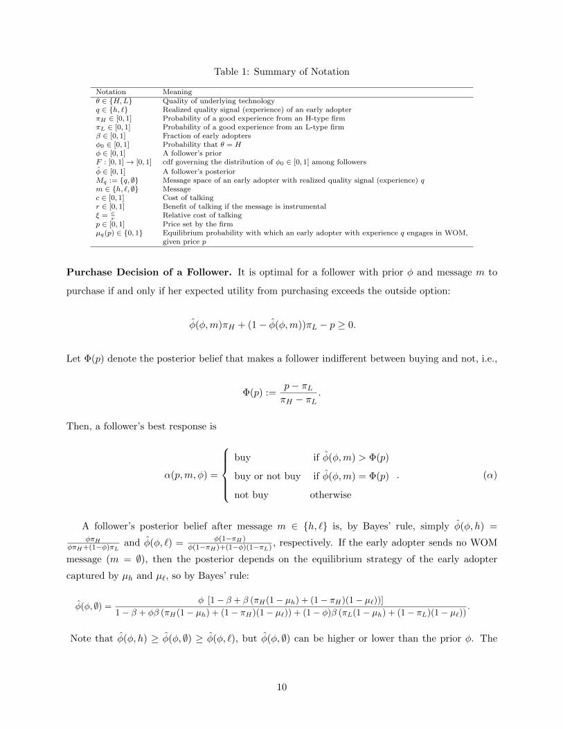
Table 1: Summary of Notation

Notation Meaningθ ∈ {H,L} Quality of underlying technologyq ∈ {h, `} Realized quality signal (experience) of an early adopterπH ∈ [0, 1] Probability of a good experience from an H-type firmπL ∈ [0, 1] Probability of a good experience from an L-type firmβ ∈ [0, 1] Fraction of early adoptersφ0 ∈ [0, 1] Probability that θ = Hφ ∈ [0, 1] A follower’s priorF : [0, 1]→ [0, 1] cdf governing the distribution of φ0 ∈ [0, 1] among followers

φ ∈ [0, 1] A follower’s posteriorMq := {q, ∅} Message space of an early adopter with realized quality signal (experience) qm ∈ {h, `, ∅} Messagec ∈ [0, 1] Cost of talkingr ∈ [0, 1] Benefit of talking if the message is instrumentalξ = c

rRelative cost of talking

p ∈ [0, 1] Price set by the firmµq(p) ∈ {0, 1} Equilibrium probability with which an early adopter with experience q engages in WOM,

given price p

Purchase Decision of a Follower. It is optimal for a follower with prior φ and message m to

purchase if and only if her expected utility from purchasing exceeds the outside option:

φ(φ,m)πH + (1− φ(φ,m))πL − p ≥ 0.

Let Φ(p) denote the posterior belief that makes a follower indifferent between buying and not, i.e.,

Φ(p) :=p− πLπH − πL

.

Then, a follower’s best response is

α(p,m, φ) =

buy if φ(φ,m) > Φ(p)

buy or not buy if φ(φ,m) = Φ(p)

not buy otherwise

. (α)

A follower’s posterior belief after message m ∈ {h, `} is, by Bayes’ rule, simply φ(φ, h) =φπH

φπH+(1−φ)πLand φ(φ, `) = φ(1−πH)

φ(1−πH)+(1−φ)(1−πL) , respectively. If the early adopter sends no WOM

message (m = ∅), then the posterior depends on the equilibrium strategy of the early adopter

captured by µh and µ`, so by Bayes’ rule:

φ(φ, ∅) =φ [1− β + β (πH(1− µh) + (1− πH)(1− µ`))]

1− β + φβ (πH(1− µh) + (1− πH)(1− µ`)) + (1− φ)β (πL(1− µh) + (1− πL)(1− µ`)).

Note that φ(φ, h) ≥ φ(φ, ∅) ≥ φ(φ, `), but φ(φ, ∅) can be higher or lower than the prior φ. The

10

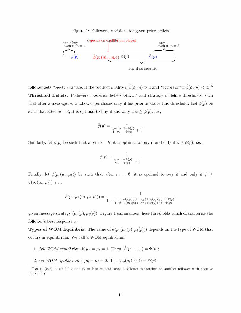
Figure 1: Followers’ decisions for given prior beliefs

0 1φ(p)φ(p) φ(p; (mh,m`)) Φ(p)

depends on equilibrium playeddon’t buyeven if m = h

buyeven if m = `

buy if no message

follower gets “good news” about the product quality if φ(φ,m) > φ and “bad news” if φ(φ,m) < φ.15

Threshold Beliefs. Followers’ posterior beliefs φ(φ,m) and strategy α define thresholds, such

that after a message m, a follower purchases only if his prior is above this threshold. Let φ(p) be

such that after m = `, it is optimal to buy if and only if φ ≥ φ(p), i.e.,

φ(p) =1

1−πH1−πL

1−Φ(p)Φ(p) + 1

.

Similarly, let φ(p) be such that after m = h, it is optimal to buy if and only if φ ≥ φ(p), i.e.,

φ(p) =1

πHπL

1−Φ(p)Φ(p) + 1

.

Finally, let φ(p; (µh, µ`)) be such that after m = ∅, it is optimal to buy if and only if φ ≥

φ(p; (µh, µ`)), i.e.,

φ(p; (µh(p), µ`(p))) =1

1 + 1−β+β(µh(p)(1−πH)+µ`(p)πH)1−β+β(µh(p)(1−πL)+µ`(p)πL)

1−Φ(p)Φ(p)

,

given message strategy (µh(p), µ`(p)). Figure 1 summarizes these thresholds which characterize the

follower’s best response α.

Types of WOM Equilibria. The value of φ(p; (µh(p), µ`(p))) depends on the type of WOM that

occurs in equilibrium. We call a WOM equilibrium

1. full WOM equilibrium if µh = µ` = 1. Then, φ(p; (1, 1)) = Φ(p);

2. no WOM equilibrium if µh = µ` = 0. Then, φ(p; (0, 0)) = Φ(p);

15m ∈ {h, `} is verifiable and m = ∅ is on-path since a follower is matched to another follower with positiveprobability.

11

3. negative WOM if µh = 0, µ` = 1. Then,

Φ(p) ≥ φ(p; (0, 1)) =1

1 + 1−β+βπH1−β+βπL

1−Φ(p)Φ(p)

;

4. positive WOM if µh = 1, µ` = 0. Then

Φ(p) ≤ φ(p; (1, 0)) =1

1 + 1−β+β(1−πH)1−β+β(1−πL)

1−Φ(p)Φ(p)

.

The absence of WOM (m = ∅) means “good news” in a negative WOM equilibrium, but

“bad news” in a positive WOM equilibrium. The number of early adopters β determines the

informativeness of m = ∅ (no WOM). It is a weaker signal, the less likely a follower is matched to

an early adopter (β small).

Early Adopter’s WOM Decision. Given the follower’s best-response described by the belief

thresholds defined above, we can infer the early adopters’ communication decisions. Assume that

F has no mass point at the thresholds φ(p), φ(p), φ(p; (µh, µ`)) for µh, µ` ∈ {0, 1}. Then, an early

adopter who observes q = h weakly prefers to engage in WOM whenever

(1− β)r(F (φ(p; (µh, µ`)))− F (φ(p)))

)︸ ︷︷ ︸benefit of talking if q=h

≥ c︸︷︷︸cost of talking

.

Similarly, if q = `, an early adopter weakly prefers to engage in WOM whenever

(1− β)r(F (φ(p))− F (φ(p; (µh, µ`))︸ ︷︷ ︸

benefit of talking if q=`

≥ c︸︷︷︸cost of talking

.

To characterize the WOM equilibrium, we call followers

• pessimistic, whenever F (Φ(p))− F (φ(p)) ≥ ξ1−β ≥ F (φ(p))− F (Φ(p));

• optimistic, whenever F (φ(p))− F (Φ(p)) ≥ ξ1−β ≥ F (Φ(p))− F (φ(p));

• uninformed whenever F (Φ(p))− F (φ(p)), F (φ(p))− F (Φ(p)) ≥ ξ1−β ;

• well-informed whenever F (Φ(p))− F (φ(p)), F (φ(p))− F (Φ(p)) ≤ ξ1−β .

Importantly, this definition is independent of the WOM equilibrium played. Followers are

said to be well-informed if most followers have extreme priors, and cannot be influenced by any

12

information from the early adopter. Followers are said to be pessimistic if, given price p, there is

a large mass of followers who have priors that are relatively low but not lower than φ(p). Note

that the beliefs of such followers are not so extreme that they never be influenced to buy. Positive

information can potentially impact their decision. In contrast, followers are said to be optimistic if

there is a sufficiently large mass of followers who have priors that are relatively high but not higher

than φ(p). The beliefs of such followers are in turn not so extreme that they will buy regardless of

information. Negative information can potentially influence them not to buy. Finally, followers are

said to be uninformed if there are many followers that can potentially be convinced to change their

purchasing behavior in both directions. Finally, note that the three categories are not mutually

exclusive in the knife-edge cases of F (Φ(p))− F (φ(p)) = ξ1−β and/or F (φ(p))− F (Φ(p)) = ξ

1−β .

Characterization of WOM Equilibria. We now characterize the WOM sub-game.

Lemma 1 (WOM sub-game) Let price p be such that F has no mass point at φ(p), φ(p),

φ(p; (µh, µ`)) for µh, µ` ∈ {0, 1}. There exist thresholds βneg(p), βpos(p) > 0 such that

1. A full WOM equilibrium exists if and only if followers are uninformed.

2. A no WOM equilibrium exists if and only if followers are well-informed.

3. A negative WOM equilibrium exists for all β ∈ [0, 1] if followers are optimistic. For

β < βneg(p), a negative WOM equilibrium does not exist if buyers are not optimistic.

4. A positive WOM equilibrium exists for all β ∈ [0, 1] if followers are pessimistic. For

β < βpos(p), a positive WOM equilibrium does not exist if buyers are not pessimistic.

An early adopter is willing to incur the cost of WOM cost only if the followers’ decision is affected

with a sufficiently high probability. Thus, with pessimistic followers, early adopters with a positive

experience have a strong incentive to talk, while those with a negative experience have a weaker

incentive. Indeed, in that case, a positive WOM equilibrium exists and m = ∅ is bad news.

Similarly, with optimistic priors a negative WOM equilibrium exists. With well-informed followers,

a large proportion of followers cannot be influenced, implying that there is no WOM. Analogously,

with uninformed followers, the unique WOM equilibrium entails full WOM.

Multiplicity arises for large β. For example, with pessimistic followers, in a positive WOM

equilibrium, m = ∅ is bad news and is almost equivalent to m = `. Thus, a negative WOM

equilibrium also exists. The case when F has mass-points at the thresholds, is considered in the

proof of Proposition 1.

13

4.2 Main Results

Finally, we consider the full game including the firm’s pricing decision. Define π(φ0) := φ0πH +

(1− φ0)πL to be the firm’s belief that an early adopter has a good experience.

4.2.1 Homogeneous Priors

We start with the benchmark case when followers share the same prior φ = φ0, i.e., F = 1(φ ≥ φ0),

because the brand is well-entrenched.

Proposition 1 (Homogeneous priors or well-entrenched brand image) Let F = 1(φ ≥ φ0).

In any pure-strategy equilibrium, negative WOM can be sustained in equilibrium if and only if

β ≤ βhom :=(1− φ0)φ0(πH − πL)2

(1− π(φ0))(π(φ0)− (φ0π2H + (1− φ0)π2

L)).

No WOM can be sustained if and only if β ≥ βhom. No other WOM equilibria can be sustained.

Intuitively, for a well-entrenched brand, the firm can set a price low enough such that all followers

buy in the absence of WOM. The firm cannot improve upon this. For small β, the firm can increase

the price if m = ∅ is a weak good signal, which is the case in a negative WOM equilibrium. Followers

who receive a negative signal will not buy, but for small β, there are only few such followers. If β

is large, negative WOM is not worthwhile because too many followers receive the negative signal.

Positive WOM is worthwhile only if the firm can charge a higher price to followers with a positive

message. However, this is dominated by no WOM, where all consumers buy.

4.2.2 Heterogeneous Priors

Next, consider heterogeneous priors with continuous F . Denote the set of profit-maximizing prices

by

P∗ = arg maxp∈[0,1]

p(1− F (Φ(p))).

Note that P∗ 6= ∅ because the prices in the set are maximizing a continuous function on a compact

set. We first focus on two extreme cases:

1. Strong brand image: For all p ∈ P∗, F (Φ(p)) < ξ.

2. Weak brand image: For all p ∈ P∗, F (Φ(p)) > ξ.

14

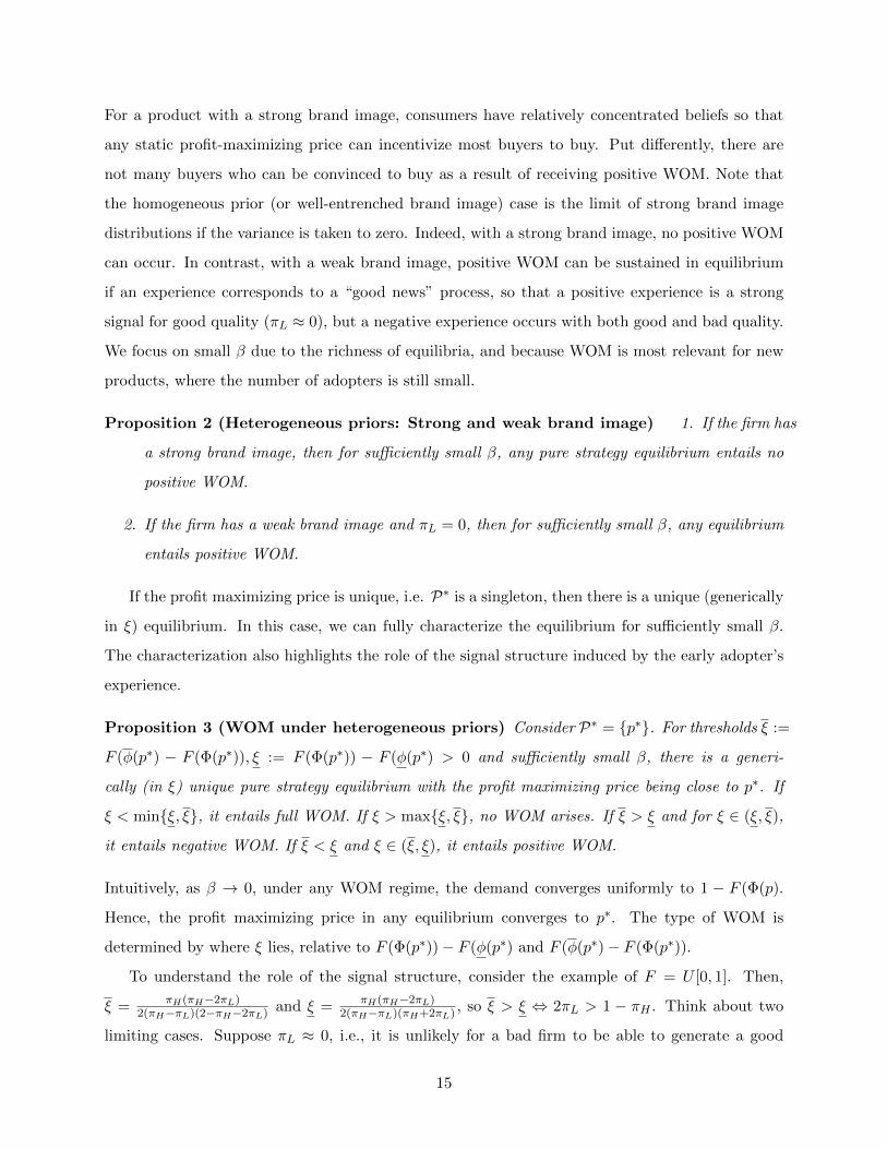
For a product with a strong brand image, consumers have relatively concentrated beliefs so that

any static profit-maximizing price can incentivize most buyers to buy. Put differently, there are

not many buyers who can be convinced to buy as a result of receiving positive WOM. Note that

the homogeneous prior (or well-entrenched brand image) case is the limit of strong brand image

distributions if the variance is taken to zero. Indeed, with a strong brand image, no positive WOM

can occur. In contrast, with a weak brand image, positive WOM can be sustained in equilibrium

if an experience corresponds to a “good news” process, so that a positive experience is a strong

signal for good quality (πL ≈ 0), but a negative experience occurs with both good and bad quality.

We focus on small β due to the richness of equilibria, and because WOM is most relevant for new

products, where the number of adopters is still small.

Proposition 2 (Heterogeneous priors: Strong and weak brand image) 1. If the firm has

a strong brand image, then for sufficiently small β, any pure strategy equilibrium entails no

positive WOM.

2. If the firm has a weak brand image and πL = 0, then for sufficiently small β, any equilibrium

entails positive WOM.

If the profit maximizing price is unique, i.e. P∗ is a singleton, then there is a unique (generically

in ξ) equilibrium. In this case, we can fully characterize the equilibrium for sufficiently small β.

The characterization also highlights the role of the signal structure induced by the early adopter’s

experience.

Proposition 3 (WOM under heterogeneous priors) Consider P∗ = {p∗}. For thresholds ξ :=

F (φ(p∗) − F (Φ(p∗)), ξ := F (Φ(p∗)) − F (φ(p∗) > 0 and sufficiently small β, there is a generi-

cally (in ξ) unique pure strategy equilibrium with the profit maximizing price being close to p∗. If

ξ < min{ξ, ξ}, it entails full WOM. If ξ > max{ξ, ξ}, no WOM arises. If ξ > ξ and for ξ ∈ (ξ, ξ),

it entails negative WOM. If ξ < ξ and ξ ∈ (ξ, ξ), it entails positive WOM.

Intuitively, as β → 0, under any WOM regime, the demand converges uniformly to 1 − F (Φ(p).

Hence, the profit maximizing price in any equilibrium converges to p∗. The type of WOM is

determined by where ξ lies, relative to F (Φ(p∗))− F (φ(p∗) and F (φ(p∗)− F (Φ(p∗)).

To understand the role of the signal structure, consider the example of F = U [0, 1]. Then,

ξ = πH(πH−2πL)2(πH−πL)(2−πH−2πL) and ξ = πH(πH−2πL)

2(πH−πL)(πH+2πL) , so ξ > ξ ⇔ 2πL > 1 − πH . Think about two

limiting cases. Suppose πL ≈ 0, i.e., it is unlikely for a bad firm to be able to generate a good

15

experience. Hence, q = h is particularly informative since it fully reveals that θ = H: Examples

are categories like independent restaurants where the consumer is discerning and is looking for

specialized qualities. In such situations, negative WOM is never optimally induced by the firm,

but positive WOM is induced for an intermediate range of WOM costs. For πL = 0 we have

ξ = πH2(2−πH) < ξ = 1

2 and ξ is increasing in πH . Thus, positive WOM is optimal for a wider range

of costs if πH is also small. Next, suppose πH ≈ 1. Then, a good firm can generate a positive

experience with high likelihood. Here, q = l is particularly informative. Car rentals might fall into

this category: Customers are happy as long as no major quality flaws such as cleanliness or terrible

service occur. If πH = 1, then ξ = 12(1−πL) > ξ = 1−2πL

2(1+πL−2π2L)

and ξ − ξ is increasing in πL, i.e.,

negative WOM is sustained for a wider range of costs if πL is large. Finally, if πH < 2πL, then the

firm induces no WOM because no signal is sufficiently informative about quality.

5 Extensions

Our baseline model is kept as lean as possible to highlight our main results, that we then test in

the data. In this section, we discuss how far our results generalize in various dimensions.

5.1 Dynamics

In our baseline model, we consider a single round of WOM decisions followed by purchasing deci-

sions. A natural extension is to allow for dynamics, where followers today may engage in WOM

tomorrow. Consider the following alternative model. As before, there is a unit mass of consumers,

and the prior belief about the firm’s unknown product quality, at the start of the game, is given

by φ0 = φ ∼ F . Time t = 0, 1, 2, . . . is discrete. At t = 0, a fraction β0 of early adopters tries

the product for free. In every subsequent period t, early adopters comprise the early adopters

from period 0 and all followers who have adopted up to period t. We denote the fraction of early

adopters in period t by βt, the belief of a follower by φt and its distribution by F t. The timing of

the dynamic game is the natural analog of the static game of the baseline model:

1. In every period t, a consumer is randomly chosen to be a potential reviewer (engage in WOM),

and a fraction ∆ > 0 of consumers is picked at random to be potential followers.

2. The firm sets a period-t net price pt.

3. If the chosen potential reviewer is not an early adopter, then there is no WOM in period t.

16

If he is an early adopter, then he has experienced a quality signal q in some period prior to

t, and can decide whether to share it or not. Payoffs of early adopters in any period t are

analogous to those in the baseline model, i.e., he receives a benefit r∆ from every follower who

adopts in that period. Formally, he engages in WOM after experiencing q = h whenever

(1− βt)r(F (φ(pt; (µh(pt), µ`(pt))))− F (φ(pt))) ≥ c

and engages in WOM after experiencing q = ` whenever

(1− βt)r(F (φ(pt))− F (φ(pt; (µh(pt), µ`(pt))))) ≥ c,

4. Finally, potential followers in period t decide whether to buy or not based on their updated

belief about quality.16 Again, analogous to our baseline model, this belief of a follower in

period t can be calculated by Bayes’ rule, using the consumer belief from period t − 1 and

the WOM message (or lack of WOM) in period t.

In this setting, both the distribution F t of priors φt and the fraction of early adopters βt are

changing over time, but the equilibrium outcome in each period is derived exactly as in our baseline

model. Thus, the results in Proposition 1 generalize. In equilibrium, negative WOM arises early

on, followed by no WOM later when βt exceeds a threshold. The results in Propositions 2 and 3

are valid in periods in which βt is sufficiently small, given the distribution F t of period-t priors φt.

5.2 More than one Follower

In a platform like Yelp, reviewers do not only review sequentially, but might also take into account

that a single review is read by multiple potential consumers in the future.17 Similar trade-offs

persist in that case.

To see this, for simplicity, consider a static model as in our baseline in which an early adopter

is matched to not one, but n > 1 followers whose prior beliefs are drawn from a distribution F .

Then, the analysis is identical, but with ξ replaced by ξn . Thus, the more followers can see a review,

the more WOM we expect. However, the type of WOM is unaffected by the number of followers n

that one receiver speaks to.

16When making a purchasing decision, followers do not take into account that they can become future early adoptersand have the opportunity to write a review.

17Note that the dynamic model above already takes into account that each follower has access to all past reviews.

17

5.3 Privately informed Firm

In the baseline model, we assumed that the firm was unaware of its quality when it set its price.

This captures situations where the firm is launching an entirely new product and does not know

about product efficacy prior to a large-scale launch. However, in other settings, the firm may be

aware of its quality at the time of its pricing decision. In this section, we consider a straightforward

extension, now with private information. For simplicity, we focus on situations with few early

adopters (small β), and the uniform distribution in the case of heterogeneous priors.

If a firm has private information about quality, then it can, in principle, signal this information

through its price, and followers may update their beliefs about the firm’s type. However, such

signaling via prices cannot arise in a pure-strategy equilibrium, i.e., there is no fully separating

equilibrium.18 To see this, let us assume that there is a fully separating equilibrium in which a H-

firm sets pH and a L-firm sets pL. In a fully separating equilibrium, both prices will be set so that

all buyers are willing to buy. Thus, if pH > pL, then the L-firm wishes to deviate to offering pH . If

pL > pH ≥ πL, then no one buys at the price pL and the L-firm can increase profits by deviating to

pH . Consequently, any pure-strategy equilibrium must be pooling, that is both firm types choose

the same price. In such an equilibrium, the posterior belief is independent of the observed price.

We characterize the unique pooling equilibrium in which the H-type firm maximizes its profits.

This equilibrium has similar features to the equilibrium constructed in Section 4. In particular,

the WOM subgame is identical and Lemma 1 applies. However, the profit function differs, as a

θ-type firm can now calibrate demand using its private information about its quality. The following

proposition is the analog to the results in the baseline model.

Proposition 4 1. Consider a setting with homogeneous priors. For sufficiently small β, firms

induce a negative WOM equilibrium in any pooling equilibrium.

2. Consider a setting with heterogeneous priors and F = U [0, 1]. For sufficiently small β, in

the H-optimal pooling equilibrium, given the same cutoff costs ξ and ξ as Proposition 3, the

equilibrium entails full WOM if ξ ≤ min{ξ, ξ} and no WOM if ξ ≥ max{ξ, ξ}. Furthermore,

• if 2πL ≥ 1− πH , then ξ ≥ ξ and for ξ ∈ [ξ, ξ] the equilibrium entails negative WOM,

• if 2πL ≤ 1− πH , then ξ ≤ ξ and for ξ ∈ [ξ, ξ] the equilibrium entails positive WOM.

18We conjecture that a semi-separating may exist if we allowed for mixed strategies.

18

To summarize, only the profit-maximizing price differs from the setting with symmetric information.

All WOM equilibria are unchanged.

5.4 Idiosyncratic Value

Finally, one might wonder how the results would change if the potential customer base had idiosyn-

cratic preferences over different products (horizontal differentiation). Suppose that the expected

utility of a follower of purchasing the product at price p is

φ(φ,m)πH + (1− φ(φ,m))πL + ε− p ≥ 0

where ε is a taste parameter distributed according to a distribution G. The cutoff beliefs Φ(p, ε),

φ(p, ε) and φ(p, ε) are functions of the realized ε and we need to categorize WOM equilibria as

• pessimistic, whenever∫F (Φ(p, ε))−F (φ(p, ε))dG(ε) ≥ ξ

1−β ≥∫F (φ(p, ε))−F (Φ(p, ε)) dG(ε);

• optimistic, whenever∫F (φ(p, ε))−F (Φ(p, ε)) dG(ε) ≥ ξ

1−β ≥∫F (Φ(p, ε))−F (φ(p, ε))dG(ε);

• uninformed whenever∫F (Φ(p, ε))−F (φ(p, ε))dG(ε),

∫F (φ(p, ε))−F (Φ(p, ε)) dG(ε) ≥ ξ

1−β ;

• well-informed whenever∫F (Φ(p))− F (φ(p))dG(ε),

∫F (φ(p))− F (Φ(p)) dG(ε) ≤ ξ

1−β .

Using this definition, Lemma 1 can be generalized. However, Proposition 1, only holds if the taste

parameter is a point-distribution as well. An analogous argument to Proposition 2 (i) can be

made only if tastes are not too dispersed. Hence, the interaction between horizontal and vertical

differentiation add some complications, but the forces uncovered in Section 4 remain present even

when we allow for some limited idiosyncratic taste.

6 Empirical Evidence

Our analysis shows that the selection of positive versus negative WOM can depend on two fac-

tors: the strength of the brand image (how dispersed priors are) and the informativeness of nega-

tive/positive experiences. A stark and testable prediction is that with homogeneous priors (well-

entrenched brand image) or close to homogeneous priors (strong brand image)no positive WOM

can arise (Propositions 1 and 2). In contrast, for a weak brand image with “good news processes”,

positive WOM arises in any equilibrium as long as the cost of WOM is not too large (Proposition

2). In this section, we examine these testable implications with data.

19

6.1 Restaurant Industry and Review Platforms

Restaurant review platforms present a good setting to validate our theoretical predictions. Restau-

rants are experience goods whose quality cannot be fully ascertained a priori (Nelson, 1970; Luca,

2016) and people often rely on recommendations from their social contacts.19 Moreover, the restau-

rant industry allows us to distinguish cleanly between homogeneous and heterogeneous priors. Prior

beliefs about restaurant quality naturally vary across consumers, and the extent to which consumers

agree depends on how they interpret the visible characteristics of a restaurant: the brand name,

cuisine, chef, etc. In this context, national chains like Subway or Domino’s Pizza have invested

millions of dollars to create a well-entrenched brand image with a clearly communicated brand

promise and product portfolio. We can thus expect people to have homogeneous beliefs about the

quality of such chain restaurants. In contrast, the industry also has smaller, independent restau-

rants that are typically one-store entities that cannot build such a clear reputation, and must start

out with more variance in consumer beliefs about their quality. We thus expect people to have

heterogeneous beliefs about the quality of independent restaurants. Existence of these two types of

restaurants is critical to testing the predictions of our model. Moreover, unlike some other product

categories which also have active review forums, like hotels, cars or movies, restaurants are quite

local, without strong loyalty programs. Hence, it is reasonable to assume that reviewers are mo-

tivated to engage in WOM because they want to be providers of useful instrumental information,

rather than by loyalty rewards or other external incentives.20

6.2 Data Description and Summary Statistics

We construct our dataset from the Yelp Data Challenge 2017 and separate chain restaurant data.

The Yelp dataset has business, review and reviewer information for restaurants in several US and

some Canadian cities (majorly Pittsburgh, Charlotte, Las Vegas, Cleveland, Phoenix and Montreal)

between the years 2004-2017. Every review in this dataset has a unique identifier, an overall rating,

review text and timestamp. Reviews can be linked to a specific reviewer and business through

unique business and reviewer identifiers. For every business, we know the name and exact location.

Likewise, for every reviewer we have information like when they joined the platform, how many

1994 % of US diners are influenced by online reviews as per the Trip Advisor “Influences in Diner Decision-Making”survey 2018. BrightLocal’s 2017 Local Consumer Review Survey estimated this number at 97 %

20Yelp.com in fact recognizes this self-enhancement motive of users, and encourages users to interact and build acommunity, through programs like Yelp Elite. We do however find some evidence that sometimes reviewers reviewto give feedback to the restaurant or a particular server.

20

years they have been part of the Yelp Elite program, number of friends and fans and how many

compliments they have received. We augment this dataset with other business characteristics like

whether the business is a chain or not (chain dummy), and for chains we add the age of the brand

and number of stores of the brand in US (from Statista.com and company websites). We also

derive the cuisine variable for a restaurant using information from corporate reports for chains and

name-matching for independent restaurants.21

The restaurants in the data cover a huge variety of cuisines; we restrict attention to cuisines for

which there exist both independent restaurants and chains. We identify 72 chains and cluster them

based on two dimensions, age of the chain and number of stores in the United States. Seven are

classified as national established chains with a median brand age of 62 years and median spread

of 15K stores per chain (in US). These seven chains are Burger King, Domino’s Pizza, Dunkin’

Donuts, KFC, McDonald’s, Pizza Hut and Subway.22 We have 30, 419 reviews from 2834 such

national established chain stores. There are two additional clusters that we combine in a category

that we call less established chains. These are either old brands with limited coverage e.g., Carl’s Jr

and Chick-fil-A or relatively newer brands and cuisines e.g., Applebee’s Neighborhood Grill & Bar,

Red Lobster and Chipotle. Their median brand age is 50 years and coverage is 1000 stores across

US. We have 86, 359 reviews from 2913 less established chains. Most of the national established

chains are sandwich, pizza, burger joints and coffee shops whereas the less established chains have a

wider variety of cuisines e.g., “delis”, “chinese”, “breakfast” and “steak”. To ensure fair comparison

between chain restaurants and independent restaurants, we chose independent restaurants serving

the same cuisines by name-matching on “sandwich”, “pizza”, “burger”,“steak”, “deli”, “breakfast

(or brunch)”, “chinese” and “coffee” categories. This gives us a total of 307,622 reviews from 6228

independent restaurants. Refer to Table 2 for a summary of the characteristics of the different

restaurant types.

6.3 Supporting Evidence from Data

6.3.1 Rating Distribution Of Chain and Independent Restaurants

We start with describing the raw data by presenting some summary statistics, and distributions of

ratings for different types of restaurants. We calculate two review statistics: the average review-

21Independent restaurants often have the cuisine in their name for e.g., Otaru Sushi or Mooyah Burgers. We ignorerestaurants for which we cannot identify the cuisine.

22Table 8 has some more details about these chains like revenue, brand value and proportion of positive, negativeand neutral word of mouth

21

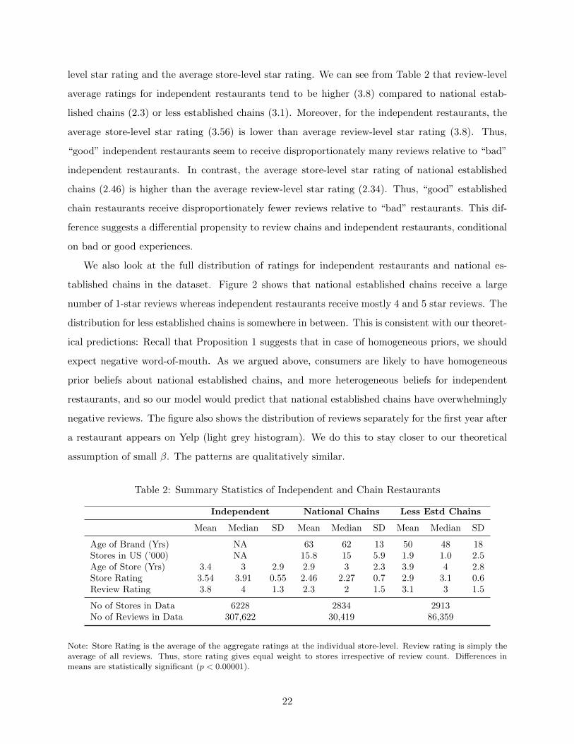
level star rating and the average store-level star rating. We can see from Table 2 that review-level

average ratings for independent restaurants tend to be higher (3.8) compared to national estab-

lished chains (2.3) or less established chains (3.1). Moreover, for the independent restaurants, the

average store-level star rating (3.56) is lower than average review-level star rating (3.8). Thus,

“good” independent restaurants seem to receive disproportionately many reviews relative to “bad”

independent restaurants. In contrast, the average store-level star rating of national established

chains (2.46) is higher than the average review-level star rating (2.34). Thus, “good” established

chain restaurants receive disproportionately fewer reviews relative to “bad” restaurants. This dif-

ference suggests a differential propensity to review chains and independent restaurants, conditional

on bad or good experiences.

We also look at the full distribution of ratings for independent restaurants and national es-

tablished chains in the dataset. Figure 2 shows that national established chains receive a large

number of 1-star reviews whereas independent restaurants receive mostly 4 and 5 star reviews. The

distribution for less established chains is somewhere in between. This is consistent with our theoret-

ical predictions: Recall that Proposition 1 suggests that in case of homogeneous priors, we should

expect negative word-of-mouth. As we argued above, consumers are likely to have homogeneous

prior beliefs about national established chains, and more heterogeneous beliefs for independent

restaurants, and so our model would predict that national established chains have overwhelmingly

negative reviews. The figure also shows the distribution of reviews separately for the first year after

a restaurant appears on Yelp (light grey histogram). We do this to stay closer to our theoretical

assumption of small β. The patterns are qualitatively similar.

Table 2: Summary Statistics of Independent and Chain Restaurants

Independent National Chains Less Estd Chains

Mean Median SD Mean Median SD Mean Median SD

Age of Brand (Yrs) NA 63 62 13 50 48 18Stores in US (’000) NA 15.8 15 5.9 1.9 1.0 2.5Age of Store (Yrs) 3.4 3 2.9 2.9 3 2.3 3.9 4 2.8Store Rating 3.54 3.91 0.55 2.46 2.27 0.7 2.9 3.1 0.6Review Rating 3.8 4 1.3 2.3 2 1.5 3.1 3 1.5

No of Stores in Data 6228 2834 2913No of Reviews in Data 307,622 30,419 86,359

Note: Store Rating is the average of the aggregate ratings at the individual store-level. Review rating is simply theaverage of all reviews. Thus, store rating gives equal weight to stores irrespective of review count. Differences inmeans are statistically significant (p < 0.00001).

22

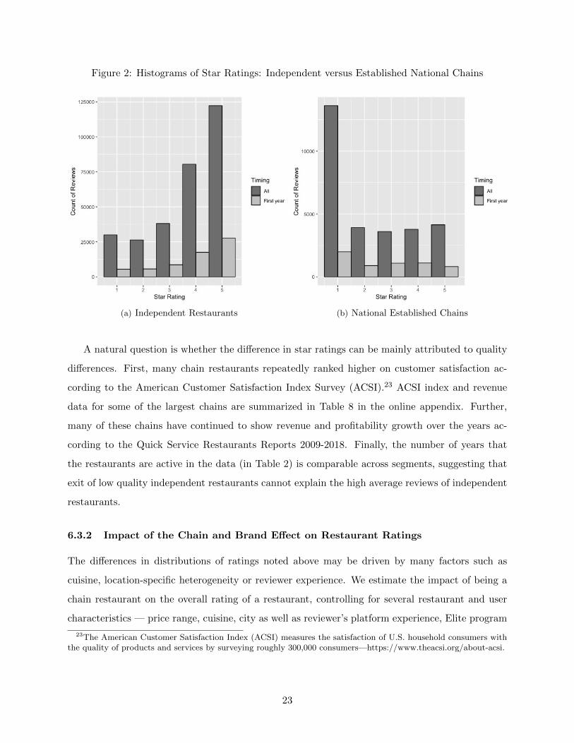
Figure 2: Histograms of Star Ratings: Independent versus Established National Chains

(a) Independent Restaurants (b) National Established Chains

A natural question is whether the difference in star ratings can be mainly attributed to quality

differences. First, many chain restaurants repeatedly ranked higher on customer satisfaction ac-

cording to the American Customer Satisfaction Index Survey (ACSI).23 ACSI index and revenue

data for some of the largest chains are summarized in Table 8 in the online appendix. Further,

many of these chains have continued to show revenue and profitability growth over the years ac-

cording to the Quick Service Restaurants Reports 2009-2018. Finally, the number of years that

the restaurants are active in the data (in Table 2) is comparable across segments, suggesting that

exit of low quality independent restaurants cannot explain the high average reviews of independent

restaurants.

6.3.2 Impact of the Chain and Brand Effect on Restaurant Ratings

The differences in distributions of ratings noted above may be driven by many factors such as

cuisine, location-specific heterogeneity or reviewer experience. We estimate the impact of being a

chain restaurant on the overall rating of a restaurant, controlling for several restaurant and user

characteristics — price range, cuisine, city as well as reviewer’s platform experience, Elite program

23The American Customer Satisfaction Index (ACSI) measures the satisfaction of U.S. household consumers withthe quality of products and services by surveying roughly 300,000 consumers—https://www.theacsi.org/about-acsi.

23

membership and reviewer-specific rating leniency. We specify

Rijt = β0 + β1 Chainj + β2Xj + β3Ui + εijt (1)

where Rijt denotes the rating of restaurant j by reviewer i at time t, Chainj captures whether

restaurant j is a chain or not, Xj includes the restaurant price range,24 cuisine and city, and Ui

captures reviewer-specific variables such as user experience in years, an Elite dummy and reviewer

average rating from other reviews. As another consistency check for our theory, we separately

estimate the impact of brand age and number of stores (coverage) for chain restaurants since these

can be proxies for the strength of the brand image and can determine the dispersion of consumer

beliefs.

Rijt = β0 + β1 Brand agejt + β3 No of storesjt + β2Xj + β3Ui + εijt (2)

Here Brand agejt measures the age of chain j at time t, and no of storesjt is the number of stores

of the chain j in US at time t. Table 3 (1) shows that being a chain restaurant results in getting

about 1 star less than a comparable independent restaurant.25 Further, Table 3 (2) shows that

the propensity to write a negative review increases with age of brand and number of stores; a 50

year old brand with thousands of stores will receive 0.5 less stars as compared to a new chain with

very few stores. The chain and brand age effects are quite resilient controlling for different user

characteristics (4 and 5 in Table 3), though the magnitude of the chain effect is slightly reduced

when we account for reviewer-specific leniency (average of reviewer’s ratings on other restaurants).26

We also estimate the impact of the chain effect on the number of positive (4-5 stars), negative (1-

2 stars) and neutral (3 stars) reviews at a business level. In particular, we run the three specifications

Count(Rev)gjt = β0 + β1 Chainj + β2Xj + β3Ui + εjt, (3)

where Count(Rev)gjt denotes the number of reviews of type g (positive, negative or neutral) that a

restaurant j receives in the first year and over its lifetime on the platform. The reviewer character-

istics Uij are averaged across all reviewers of a restaurant j. The results are summarized in Table 4.

A chain restaurant receives 8 less positive reviews in its first year than a comparable independent

restaurant and 26 less positive reviews over its entire lifetime. Coupled with the fact that chains

24Price is not the absolute price but rather a user’s perception of restaurant’s price range.25We also ran the same regression (1) with only first-year reviews and the coefficients remain similar.26There could be an impact of local competition. However, it is not straightforward to define the competition set

for a restaurant. So instead, we control for location(city) that captures some of this effect.

24

are less likely to receive any type of reviews, this is a large number of reviews and can sufficiently

alter the search outcomes in a platform like Yelp.com where users rely mostly on average ratings

and more recent reviews for sorting.

6.3.3 Brand Image and Beliefs: Textual Analysis of Reviews

Our premise is that the overwhelmingly negative WOM observed in chains is driven by the existence

of homogeneous consumer beliefs about the brand: Negative reviews reflect deviations from what

consumers collectively expect from the chain. For independent restaurants, consumers know that

they do not share the same expectations, so the reference to expectations is less meaningful. If

this premise is correct, a higher proportion of reviews from chain restaurants should contain words

related to expectation or belief as compared to independent restaurants. Moreover, we hypothesize

that these words are more likely to be present in negative reviews of chain restaurants.

To verify these hypotheses, we examine the textual content of a subset of randomly selected

750 reviews. We are interested in how the review text differs for positive (4-5 stars), negative (1-2

stars) and neutral (3-star) reviews of chains and independent restaurants. We create a custom

dictionary of expectation words and use it to look for instances when people mention prior beliefs

and expectations in the review text. Examples of these words would be “expect”, “past”, “im-

prove”, “decline” to name a few. We also use the pre-built LIWC dictionary (Pennebaker, 1997)

to identify mentions of discrepancies in review text which capture deviation from expectations.27

LIWC is a widely-used dictionary in psychology and marketing and examples of discrepancy words

include “should”, “could”, “would have”. Together, our custom dictionary of expectation and the

LIWC discrepancy keyword list would be able to identify instances of mentions of past notions

and deviations from belief. We also construct a custom dictionary of novelty which would identify

mentions of “novel experiences” and being “surprised.”

Table 5 shows the proportion of reviews, by restaurant type and valence, that contain mentions

of expectation, novelty and discrepancy. We can see that negative reviews of chains are most likely

to have expect words (33% of all negative chain reviews). However, positive reviews of chains

are also more likely to have expect words in comparison to independent restaurant reviews (25%

versus 16-18% in independent restaurants). This is consistent with our assumption of homogeneous

and strong priors for branded chain restaurants. Neutral reviews in general contain more expect

words (which is not surprising as a 3-star most often means that the restaurant met expectations).

27See Appendix Table 9 for our dictionaries of expectation,novelty and employee words.

25

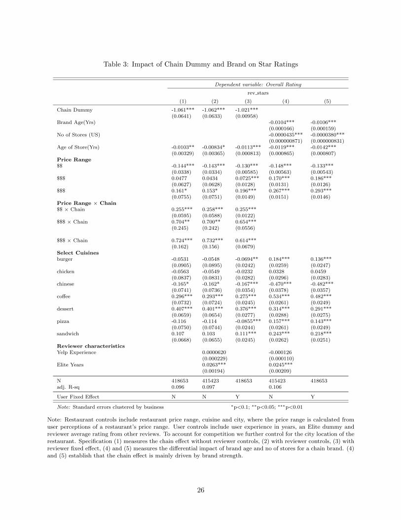
Table 3: Impact of Chain Dummy and Brand on Star Ratings

Dependent variable: Overall Rating

rev stars

(1) (2) (3) (4) (5)

Chain Dummy -1.061*** -1.062*** -1.021***(0.0641) (0.0633) (0.00958)

Brand Age(Yrs) -0.0104*** -0.0106***(0.000166) (0.000159)

No of Stores (US) -0.0000435*** -0.0000380***(0.000000871) (0.000000831)

Age of Store(Yrs) -0.0103** -0.00834* -0.0113*** -0.0119*** -0.0142***(0.00329) (0.00365) (0.000813) (0.000865) (0.000807)

Price Range$$ -0.144*** -0.143*** -0.130*** -0.148*** -0.133***

(0.0338) (0.0334) (0.00585) (0.00563) (0.00543)$$$ 0.0477 0.0434 0.0725*** 0.170*** 0.186***

(0.0627) (0.0628) (0.0128) (0.0131) (0.0126)$$$ 0.161* 0.153* 0.196*** 0.267*** 0.293***

(0.0755) (0.0751) (0.0149) (0.0151) (0.0146)Price Range × Chain$$ × Chain 0.255*** 0.258*** 0.255***

(0.0595) (0.0588) (0.0122)$$$ × Chain 0.704** 0.700** 0.654***

(0.245) (0.242) (0.0556)

$$$ × Chain 0.724*** 0.732*** 0.614***(0.162) (0.156) (0.0679)

Select Cuisinesburger -0.0531 -0.0548 -0.0694** 0.184*** 0.136***

(0.0905) (0.0895) (0.0242) (0.0259) (0.0247)chicken -0.0563 -0.0549 -0.0232 0.0328 0.0459

(0.0837) (0.0831) (0.0282) (0.0296) (0.0283)chinese -0.165* -0.162* -0.167*** -0.470*** -0.482***

(0.0741) (0.0736) (0.0354) (0.0378) (0.0357)coffee 0.296*** 0.293*** 0.275*** 0.534*** 0.482***

(0.0732) (0.0724) (0.0245) (0.0261) (0.0249)dessert 0.407*** 0.401*** 0.376*** 0.314*** 0.291***

(0.0659) (0.0654) (0.0277) (0.0288) (0.0275)pizza -0.116 -0.114 -0.0855*** 0.157*** 0.143***

(0.0750) (0.0744) (0.0244) (0.0261) (0.0249)sandwich 0.107 0.103 0.111*** 0.243*** 0.218***

(0.0668) (0.0655) (0.0245) (0.0262) (0.0251)Reviewer characteristicsYelp Experience 0.0000620 -0.000126

(0.000229) (0.000110)Elite Years 0.0263*** 0.0245***

(0.00194) (0.00209)

N 418653 415423 418653 415423 418653adj. R-sq 0.096 0.097 0.106

User Fixed Effect N N Y N Y

Note: Standard errors clustered by business ∗p<0.1; ∗∗p<0.05; ∗∗∗p<0.01

Note: Restaurant controls include restaurant price range, cuisine and city, where the price range is calculated fromuser perceptions of a restaurant’s price range. User controls include user experience in years, an Elite dummy andreviewer average rating from other reviews. To account for competition we further control for the city location of therestaurant. Specification (1) measures the chain effect without reviewer controls, (2) with reviewer controls, (3) withreviewer fixed effect, (4) and (5) measures the differential impact of brand age and no of stores for a chain brand. (4)and (5) establish that the chain effect is mainly driven by brand strength.

26

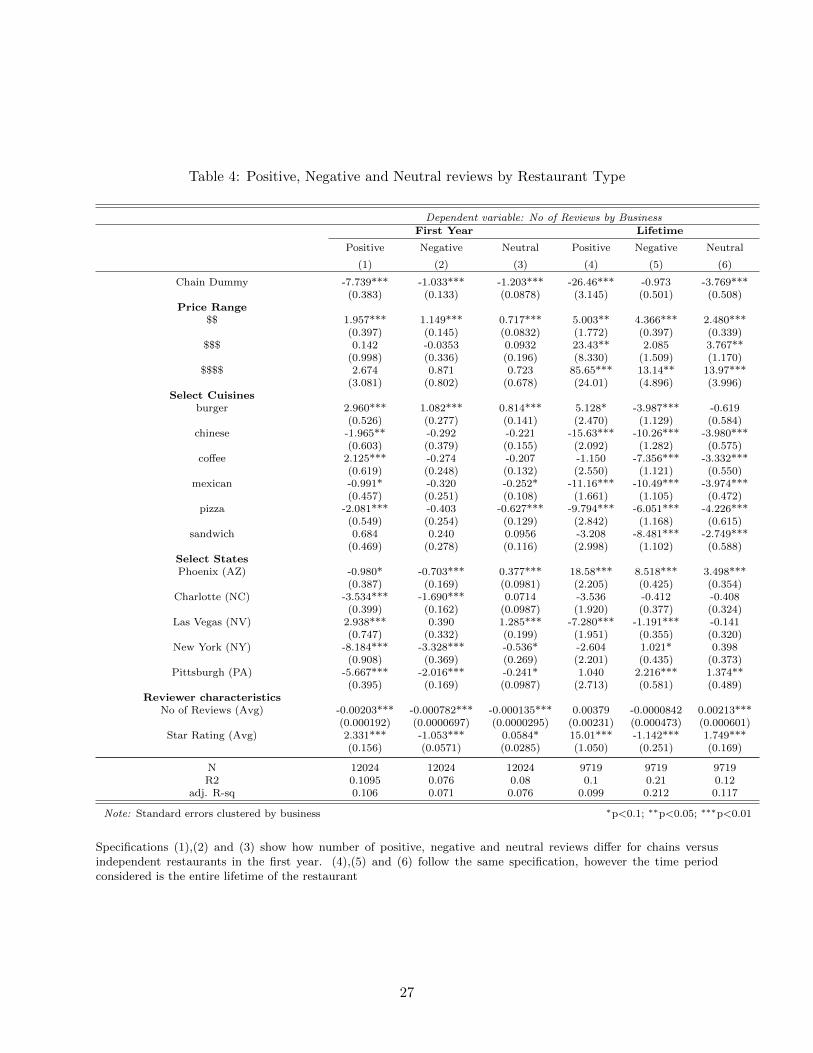
Table 4: Positive, Negative and Neutral reviews by Restaurant Type

Dependent variable: No of Reviews by BusinessFirst Year Lifetime

Positive Negative Neutral Positive Negative Neutral

(1) (2) (3) (4) (5) (6)

Chain Dummy -7.739*** -1.033*** -1.203*** -26.46*** -0.973 -3.769***(0.383) (0.133) (0.0878) (3.145) (0.501) (0.508)

Price Range$$ 1.957*** 1.149*** 0.717*** 5.003** 4.366*** 2.480***

(0.397) (0.145) (0.0832) (1.772) (0.397) (0.339)$$$ 0.142 -0.0353 0.0932 23.43** 2.085 3.767**

(0.998) (0.336) (0.196) (8.330) (1.509) (1.170)$$$$ 2.674 0.871 0.723 85.65*** 13.14** 13.97***

(3.081) (0.802) (0.678) (24.01) (4.896) (3.996)Select Cuisines

burger 2.960*** 1.082*** 0.814*** 5.128* -3.987*** -0.619(0.526) (0.277) (0.141) (2.470) (1.129) (0.584)

chinese -1.965** -0.292 -0.221 -15.63*** -10.26*** -3.980***(0.603) (0.379) (0.155) (2.092) (1.282) (0.575)

coffee 2.125*** -0.274 -0.207 -1.150 -7.356*** -3.332***(0.619) (0.248) (0.132) (2.550) (1.121) (0.550)

mexican -0.991* -0.320 -0.252* -11.16*** -10.49*** -3.974***(0.457) (0.251) (0.108) (1.661) (1.105) (0.472)

pizza -2.081*** -0.403 -0.627*** -9.794*** -6.051*** -4.226***(0.549) (0.254) (0.129) (2.842) (1.168) (0.615)

sandwich 0.684 0.240 0.0956 -3.208 -8.481*** -2.749***(0.469) (0.278) (0.116) (2.998) (1.102) (0.588)

Select StatesPhoenix (AZ) -0.980* -0.703*** 0.377*** 18.58*** 8.518*** 3.498***

(0.387) (0.169) (0.0981) (2.205) (0.425) (0.354)Charlotte (NC) -3.534*** -1.690*** 0.0714 -3.536 -0.412 -0.408

(0.399) (0.162) (0.0987) (1.920) (0.377) (0.324)Las Vegas (NV) 2.938*** 0.390 1.285*** -7.280*** -1.191*** -0.141

(0.747) (0.332) (0.199) (1.951) (0.355) (0.320)New York (NY) -8.184*** -3.328*** -0.536* -2.604 1.021* 0.398

(0.908) (0.369) (0.269) (2.201) (0.435) (0.373)Pittsburgh (PA) -5.667*** -2.016*** -0.241* 1.040 2.216*** 1.374**

(0.395) (0.169) (0.0987) (2.713) (0.581) (0.489)Reviewer characteristics

No of Reviews (Avg) -0.00203*** -0.000782*** -0.000135*** 0.00379 -0.0000842 0.00213***(0.000192) (0.0000697) (0.0000295) (0.00231) (0.000473) (0.000601)

Star Rating (Avg) 2.331*** -1.053*** 0.0584* 15.01*** -1.142*** 1.749***(0.156) (0.0571) (0.0285) (1.050) (0.251) (0.169)

N 12024 12024 12024 9719 9719 9719R2 0.1095 0.076 0.08 0.1 0.21 0.12

adj. R-sq 0.106 0.071 0.076 0.099 0.212 0.117

Note: Standard errors clustered by business ∗p<0.1; ∗∗p<0.05; ∗∗∗p<0.01

Specifications (1),(2) and (3) show how number of positive, negative and neutral reviews differ for chains versusindependent restaurants in the first year. (4),(5) and (6) follow the same specification, however the time periodconsidered is the entire lifetime of the restaurant

27

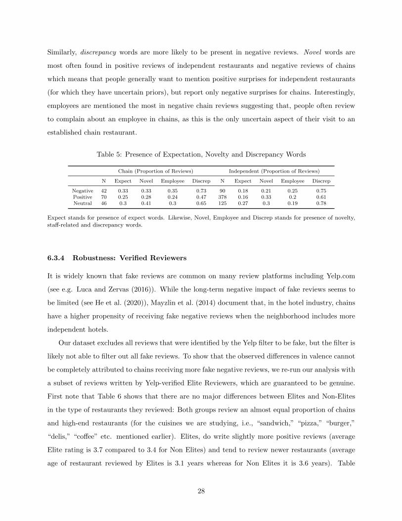
Similarly, discrepancy words are more likely to be present in negative reviews. Novel words are

most often found in positive reviews of independent restaurants and negative reviews of chains

which means that people generally want to mention positive surprises for independent restaurants

(for which they have uncertain priors), but report only negative surprises for chains. Interestingly,

employees are mentioned the most in negative chain reviews suggesting that, people often review

to complain about an employee in chains, as this is the only uncertain aspect of their visit to an

established chain restaurant.

Table 5: Presence of Expectation, Novelty and Discrepancy Words

Chain (Proportion of Reviews) Independent (Proportion of Reviews)

N Expect Novel Employee Discrep N Expect Novel Employee Discrep

Negative 42 0.33 0.33 0.35 0.73 90 0.18 0.21 0.25 0.75Positive 70 0.25 0.28 0.24 0.47 378 0.16 0.33 0.2 0.61Neutral 46 0.3 0.41 0.3 0.65 125 0.27 0.3 0.19 0.78

Expect stands for presence of expect words. Likewise, Novel, Employee and Discrep stands for presence of novelty,staff-related and discrepancy words.

6.3.4 Robustness: Verified Reviewers

It is widely known that fake reviews are common on many review platforms including Yelp.com

(see e.g. Luca and Zervas (2016)). While the long-term negative impact of fake reviews seems to

be limited (see He et al. (2020)), Mayzlin et al. (2014) document that, in the hotel industry, chains

have a higher propensity of receiving fake negative reviews when the neighborhood includes more

independent hotels.

Our dataset excludes all reviews that were identified by the Yelp filter to be fake, but the filter is

likely not able to filter out all fake reviews. To show that the observed differences in valence cannot

be completely attributed to chains receiving more fake negative reviews, we re-run our analysis with

a subset of reviews written by Yelp-verified Elite Reviewers, which are guaranteed to be genuine.

First note that Table 6 shows that there are no major differences between Elites and Non-Elites

in the type of restaurants they reviewed: Both groups review an almost equal proportion of chains

and high-end restaurants (for the cuisines we are studying, i.e., “sandwich,” “pizza,” “burger,”

“delis,” “coffee” etc. mentioned earlier). Elites, do write slightly more positive reviews (average

Elite rating is 3.7 compared to 3.4 for Non Elites) and tend to review newer restaurants (average

age of restaurant reviewed by Elites is 3.1 years whereas for Non Elites it is 3.6 years). Table

28

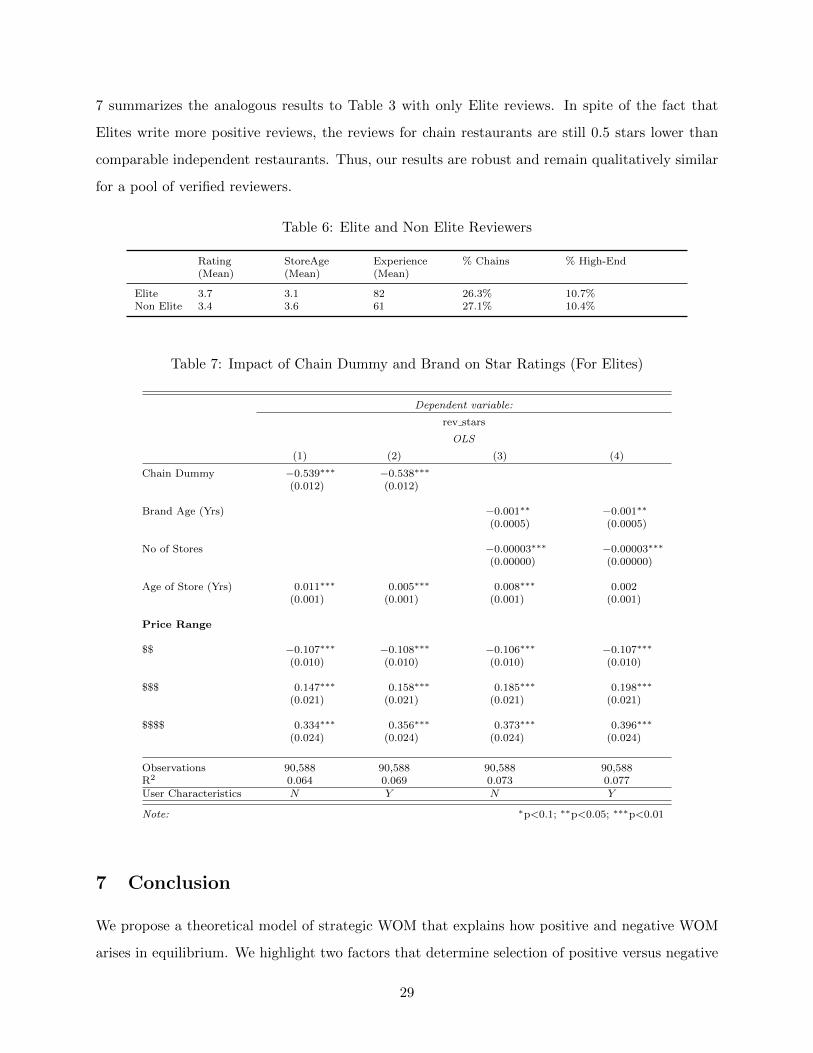
7 summarizes the analogous results to Table 3 with only Elite reviews. In spite of the fact that

Elites write more positive reviews, the reviews for chain restaurants are still 0.5 stars lower than

comparable independent restaurants. Thus, our results are robust and remain qualitatively similar

for a pool of verified reviewers.

Table 6: Elite and Non Elite Reviewers

Rating(Mean)

StoreAge(Mean)

Experience(Mean)

% Chains % High-End

Elite 3.7 3.1 82 26.3% 10.7%Non Elite 3.4 3.6 61 27.1% 10.4%

Table 7: Impact of Chain Dummy and Brand on Star Ratings (For Elites)

Dependent variable:

rev stars

OLS

(1) (2) (3) (4)

Chain Dummy −0.539∗∗∗ −0.538∗∗∗

(0.012) (0.012)

Brand Age (Yrs) −0.001∗∗ −0.001∗∗

(0.0005) (0.0005)

No of Stores −0.00003∗∗∗ −0.00003∗∗∗

(0.00000) (0.00000)

Age of Store (Yrs) 0.011∗∗∗ 0.005∗∗∗ 0.008∗∗∗ 0.002(0.001) (0.001) (0.001) (0.001)

Price Range

$$ −0.107∗∗∗ −0.108∗∗∗ −0.106∗∗∗ −0.107∗∗∗

(0.010) (0.010) (0.010) (0.010)

$$$ 0.147∗∗∗ 0.158∗∗∗ 0.185∗∗∗ 0.198∗∗∗

(0.021) (0.021) (0.021) (0.021)

$$$$ 0.334∗∗∗ 0.356∗∗∗ 0.373∗∗∗ 0.396∗∗∗

(0.024) (0.024) (0.024) (0.024)

Observations 90,588 90,588 90,588 90,588R2 0.064 0.069 0.073 0.077User Characteristics N Y N Y

Note: ∗p<0.1; ∗∗p<0.05; ∗∗∗p<0.01

7 Conclusion

We propose a theoretical model of strategic WOM that explains how positive and negative WOM

arises in equilibrium. We highlight two factors that determine selection of positive versus negative

29

WOM — the strength of the brand image as measured by the dispersion of beliefs about quality,

and the informativeness of good and bad experiences. The brand image affects how many customers

the firm can attract given its profit-maximizing price, which in-turn impacts how many consumers

can be influenced by WOM.

On platforms like Yelp.com, users rely mostly on average ratings to sort. A practical implication

of our results is that since the propensity to review varies after good or bad experiences based on the

brand image, average reviews are not a reliable measure to compare quality across restaurants.28.

More specifically, WOM needs to be interpreted differently for different types of restaurants, and

it can be problematic to use only rating comparisons on review platforms to make purchasing

decisions. Solutions can be to incentivize all consumers to write reviews, or to present more

sophisticated aggregated ratings that control for systematic selection in reviews.

Finally, our research has important implications for understanding the link between“conversational

motives” and outcomes like valence. We find that the text in the reviews can help identify the mo-

tivation of the reviewer (expectation deviance or reporting novel experiences). Text analysis can

be useful more generally to identify drivers of selection issues in reviews, and to control for them.

We leave the questions around optimal design of review aggregation mechanisms and a broader

understanding of WOM motives for future research.

28Jin, Lee, Luca et al. (2018) also highlight the disadvantages of focusing on average ratings alone and define anadjusted average that accounts for reviewer heterogeneity and past ratings

30

References

Angelis, Matteo De, Andrea Bonezzi, Alessandro M Peluso, Derek D Rucker, and

Michele Costabile, “On braggarts and gossips: A self-enhancement account of word-of-mouth

generation and transmission,” Journal of Marketing Research, 2012, 49 (4), 551–563.

Bass, Frank M, “A new product growth for model consumer durables,” Management science,

1969, 15 (5), 215–227.

Berger, Jonah, “Word of mouth and interpersonal communication: A review and directions for

future research,” Journal of Consumer Psychology, 2014, 24 (4), 586–607.

Biyalogorsky, Eyal, Eitan Gerstner, and Barak Libai, “Customer referral management:

Optimal reward programs,” Marketing Science, 2001, 20 (1), 82–95.

Campbell, Arthur, “Word-of-mouth communication and percolation in social networks,” Amer-

ican Economic Review, 2013, 103 (6), 2466–98.

, Dina Mayzlin, and Jiwoong Shin, “Managing buzz,” The RAND Journal of Economics,

2017, 48 (1), 203–229.

Carman, Ashley, “Why do you leave restaurant reviews?,” The Verge, 2018. accessed July 27,

2020.

Chakraborty, Ishita, Minkyung Kim, and K Sudhir, “Attribute Sentiment Scoring with

Online Text Reviews: Accounting for Language Structure and Attribute Self-Selection,” Cowles

Foundation Discussion Paper, 2019.

Chevalier, Judith A and Dina Mayzlin, “The effect of word of mouth on sales: Online book

reviews,” Journal of marketing research, 2006, 43 (3), 345–354.

Chintagunta, Pradeep K, Shyam Gopinath, and Sriram Venkataraman, “The effects

of online user reviews on movie box office performance: Accounting for sequential rollout and

aggregation across local markets,” Marketing Science, 2010, 29 (5), 944–957.

Dhar, Vasant and Elaine A Chang, “Does chatter matter? The impact of user-generated

content on music sales,” Journal of Interactive Marketing, 2009, 23 (4), 300–307.

31

Duan, Wenjing, Bin Gu, and Andrew B Whinston, “Do online reviews matter?—An em-

pirical investigation of panel data,” Decision support systems, 2008, 45 (4), 1007–1016.

Fradkin, Andrey, Elena Grewal, Dave Holtz, and Matthew Pearson, “Bias and reciprocity

in online reviews: Evidence from field experiments on airbnb,” in “Proceedings of the Sixteenth

ACM Conference on Economics and Computation” ACM 2015, pp. 641–641.

Galeotti, Andrea, “Talking, searching, and pricing*,” International Economic Review, 2010, 51

(4), 1159–1174.

and Sanjeev Goyal, “Influencing the influencers: a theory of strategic diffusion,” The RAND

Journal of Economics, 2009, 40 (3), 509–532.

Gilchrist, Duncan Sheppard and Emily Glassberg Sands, “Something to Talk About: Social

Spillovers in Movie Consumption,” Journal of Political Economy, 2016, 124 (5), 1339–1382.

Godes, David, “Product policy in markets with word-of-mouth communication,” Management

Science, 2016, 63 (1), 267–278.

, Dina Mayzlin, Yubo Chen, Sanjiv Das, Chrysanthos Dellarocas, Bruce Pfeiffer,

Barak Libai, Subrata Sen, Mengze Shi, and Peeter Verlegh, “The firm’s management of

social interactions,” Marketing Letters, 2005, 16 (3), 415–428.

Grice, H Paul, Peter Cole, Jerry Morgan et al., “Logic and conversation,” 1975, 1975,

pp. 41–58.

He, Sherry, Brett Hollenbeck, and Davide Proserpio, “The market for fake reviews,” Avail-

able at SSRN, 2020.

Hollenbeck, Brett, “Online reputation mechanisms and the decreasing value of chain affiliation,”

Journal of Marketing Research, 2018, 55 (5), 636–654.

Jin, Ginger, Jungmin Lee, Michael Luca et al., “Aggregation of consumer ratings: an

application to Yelp. com,” Quantitative Marketing and Economics, 2018, 16 (3), 289–339.

Kamada, Yuichiro and Aniko Ory, “Contracting with Word-of-Mouth Management,” Cowles

Foundation Discussion Paper No. 2048, 2017.

32

Ke, T. Tony, Jiwoong Shin, and Jungju Yu, “A Model of Brand Positioning: Product-

Portfolio View,” working paper, 2020.

Kornish, Laura J. and Qiuping Li, “Optimal Referral Bonuses with Asymmetric Information:

Firm-Offered and Interpersonal Incentives,” Marketing Science, 2010, 29 (1), 108–121.

Kotler, Philip, Marketing Management: The Millennium Edition, Prentice Hall, Inc., 2000.

Leduc, Matt V, Matthew O Jackson, and Ramesh Johari, “Pricing and referrals in diffusion

on networks,” Games and Economic Behavior, 2017, 104, 568–594.

Liu, Xiao, Dokyun Lee, and Kannan Srinivasan, “Large-scale cross-category analysis of

consumer review content on sales conversion leveraging deep learning,” Journal of Marketing

Research, 2019, 56 (6), 918–943.

Luca, Michael, “Reviews, reputation, and revenue: The case of Yelp.com,” Com (March 15,

2016). Harvard Business School NOM Unit Working Paper, 2016, (12-016).

and Georgios Zervas, “Fake it till you make it: Reputation, competition, and Yelp review

fraud,” Management Science, 2016, 62 (12), 3412–3427.

Luo, Xueming, “Quantifying the long-term impact of negative word of mouth on cash flows and

stock prices,” Marketing Science, 2009, 28 (1), 148–165.

Mayzlin, Dina and Jiwoong Shin, “Uninformative advertising as an invitation to search,”

Marketing Science, 2011, 30 (4), 666–685.

, Yaniv Dover, and Judith Chevalier, “Promotional reviews: An empirical investigation of

online review manipulation,” The American Economic Review, 2014, 104 (8), 2421–2455.

Mittal, Vikas, William T Ross Jr, and Patrick M Baldasare, “The asymmetric impact of

negative and positive attribute-level performance on overall satisfaction and repurchase inten-

tions,” Journal of marketing, 1998, 62 (1), 33–47.

Nelson, Phillip, “Information and Consumer Behavior,” Journal of Political Economy, 1970, 78

(2), 311–329.

Nosko, Chris and Steven Tadelis, “The limits of reputation in platform markets: An empirical

analysis and field experiment,” Technical Report, National Bureau of Economic Research 2015.

33

Onishi, Hiroshi and Puneet Manchanda, “Marketing activity, blogging and sales,” Interna-

tional Journal of Research in Marketing, 2012, 29 (3), 221–234.

Pennebaker, James W, “Writing about emotional experiences as a therapeutic process,” Psy-

chological science, 1997, 8 (3), 162–166.

Reimers, Imke C and Joel Waldfogel, “Digitization and pre-purchase information: the causal

and welfare impacts of reviews and crowd ratings,” American Economic Review (forthcoming),

2021.

Schoenmuller, Verena, Oded Netzer, and Florian Stahl, “The extreme distribution of online

reviews: Prevalence, drivers and implications,” Journal of Marketing Research, forthcoming.

Seiler, Stephan, Song Yao, and Wenbo Wang, “Does Online Word of Mouth Increase De-

mand?(And How?) Evidence from a Natural Experiment,” Marketing Science, 2017.

Sun, Monic, “How does the variance of product ratings matter?,” Management Science, 2012, 58

(4), 696–707.

A Appendix: Data

A.1 Top National Chains (2017)

34

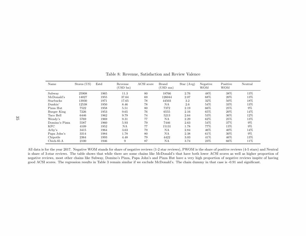
Table 8: Revenue, Satisfaction and Review Valence

Name Stores (US) Estd Revenue(USD bn)

ACSI score Brand(USD mn)

Star (Avg) NegativeWOM

PositiveWOM

Neutral

Subway 25908 1965 11.3 80 18766 2.76 48% 38% 13%McDonald’s 14027 1955 37.64 69 126044 2.07 68% 20% 13%Starbucks 13930 1971 17.65 78 44503 3.2 32% 50% 18%Dunkin’ 12538 1950 8.46 78 NA 2.6 54% 33% 13%Pizza Hut 7522 1958 5.51 80 7372 2.19 66% 25% 9%Burger King 7226 1953 9.65 76 6555 2.16 65% 20% 14%Taco Bell 6446 1962 9.79 74 5213 2.64 53% 36% 12%Wendy’s 5769 1969 9.31 77 NA 2.29 62% 25% 13%Domino’s Pizza 5587 1960 5.93 79 7446 2.63 54% 37% 9%KFC 4109 1952 NA 77 15131 1.78 77% 13% 9%Arby’s 3415 1964 3.63 79 NA 2.84 46% 40% 14%Papa John’s 3314 1984 1.78 80 NA 2.38 61% 30% 9%Chipotle 2364 1993 4.48 79 4422 3.03 41% 46% 13%Chick-fil-A 2100 1946 9 87 NA 3.74 23% 66% 11%

All data is for the year 2017. Negative WOM stands for share of negative reviews (1-2 star reviews), PWOM is the share of positive reviews (4-5 stars) and Neutralis share of 3-star reviews. The table shows that while there are some chains like McDonald’s that have both lower ACSI scores as well as higher proportion ofnegative reviews, most other chains like Subway, Domino’s Pizza, Papa John’s and Pizza Hut have a very high proportion of negative reviews inspite of havinggood ACSI scores. The regression results in Table 3 remain similar if we exclude McDonald’s. The chain dummy in that case is -0.91 and significant.

35

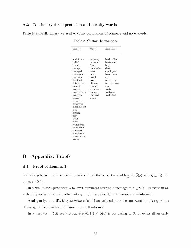
A.2 Dictionary for expectation and novelty words

Table 9 is the dictionary we used to count occurrences of compare and novel words.

Table 9: Custom Dictionaries

Expect Novel Employee

anticipate curiosity back officebelief curious bartenderbrand fresh boychange innovative deskchanged learn employeeconsistent new front deskcontrary novel girldeclined now receptiondeteriorate offbeat receptionistexceed recent staffexpect surprised waiterexpectation unique waitressexpected unusual wait-staffimage weirdimproveimprovedinconsistentmetnotionpastpriorrecallrememberreputationstandardstandardsunexpectedworsen

B Appendix: Proofs

B.1 Proof of Lemma 1

Let price p be such that F has no mass point at the belief thresholds φ(p), φ(p), φ(p; (µh, µ`)) for

µh, µ` ∈ {0, 1}.

In a full WOM equilibrium, a follower purchases after an ∅-message iff φ ≥ Φ(p). It exists iff an

early adopter wants to talk after both q = `, h, i.e., exactly iff followers are uninformed.

Analogously, a no WOM equilibrium exists iff an early adopter does not want to talk regardless

of his signal, i.e., exactly iff followers are well-informed.

In a negative WOM equilibrium, φ(p; (0, 1)) ≤ Φ(p) is decreasing in β. It exists iff an early

36

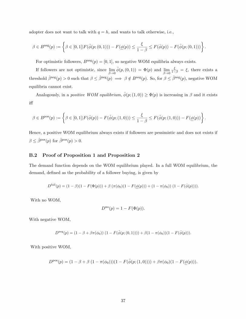
adopter does not want to talk with q = h, and wants to talk otherwise, i.e.,

β ∈ Bneg(p) :=

{β ∈ [0, 1]|F (φ(p; (0, 1)))− F (φ(p)) ≤ ξ

1− β≤ F (φ(p))− F (φ(p; (0, 1)))

}.

For optimistic followers, Bneg(p) = [0, 1], so negative WOM equilibria always exists.

If followers are not optimistic, since limβ→0

φ(p, (0, 1)) = Φ(p) and limβ→0

ξ1−β = ξ, there exists a

threshold βneg(p) > 0 such that β ≤ βneg(p) =⇒ β /∈ Bneg(p). So, for β ≤ βneg(p), negative WOM

equilibria cannot exist.

Analogously, in a positive WOM equilibrium, φ(p; (1, 0)) ≥ Φ(p) is increasing in β and it exists

iff

β ∈ Bpos(p) :=

{β ∈ [0, 1]|F (φ(p))− F (φ(p; (1, 0))) ≤ ξ

1− β≤ F (φ(p; (1, 0)))− F (φ(p))

}.

Hence, a positive WOM equilibrium always exists if followers are pessimistic and does not exists if

β ≤ βpos(p) for βpos(p) > 0.

B.2 Proof of Proposition 1 and Proposition 2

The demand function depends on the WOM equilibrium played. In a full WOM equilibrium, the

demand, defined as the probability of a follower buying, is given by

Dfull(p) = (1− β)(1− F (Φ(p))) + β (π(φ0)(1− F (φ(p))) + (1− π(φ0)) (1− F (φ(p)))).

With no WOM,

Dno(p) = 1− F (Φ(p)).

With negative WOM,

Dneg(p) = (1− β + βπ(φ0)) (1− F (φ(p; (0, 1)))) + β(1− π(φ0))(1− F (φ(p))).

With positive WOM,

Dpos(p) = (1− β + β (1− π(φ0)))(1− F (φ(p; (1, 0)))) + βπ(φ0)(1− F (φ(p))).

37

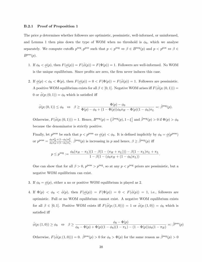
B.2.1 Proof of Proposition 1

The price p determines whether followers are optimistic, pessimistic, well-informed, or uninformed,

and Lemma 1 then pins down the type of WOM when no threshold is φ0, which we analyse

separately. We compute cutoffs pneg, ppos such that p < pneg ⇔ β ∈ Bneg(p) and p < ppos ⇔ β ∈

Bpos(p).

1. If φ0 < φ(p), then F (φ(p)) = F (φ(p)) = F (Φ(p)) = 1. Followers are well-informed. No WOM

is the unique equilibrium. Since profits are zero, the firm never induces this case.

2. If φ(p) < φ0 < Φ(p), then F (φ(p)) = 0 < F (Φ(p)) = F (φ(p)) = 1. Followers are pessimistic.

A positive WOM equilibrium exists for all β ∈ [0, 1]. Negative WOM arises iff F (φ(p; (0, 1))) =

0 or φ(p; (0, 1)) = φ0 which is satisfied iff

φ(p; (0, 1)) ≤ φ0 ⇔ β ≥ Φ(p)− φ0

Φ(p)− φ0 + (1− Φ(p))φ0πH − Φ(p)(1− φ0)πL=: βneg(p).

Otherwise, F (φ(p; (0, 1))) = 1. Hence, Bneg(p) =(βneg(p), 1−ξ

]and βneg(p) > 0 if Φ(p) > φ0

because the denominator is strictly positive.

Finally, let ppess be such that p < ppess ⇔ φ(p) < φ0. It is defined implicitly by φ0 = φ(ppess)

or ppess =φ0π2

H+(1−φ0)π2L

φ0πH+(1−φ0)πL. βneg(p) is increasing in p and hence, β ≥ βneg(p) iff

p ≤ pneg :=φ0(πH − πL)(1− β(1− (πH + πL)))− β(1− πL)πL + πL

1− β(1− (φ0πH + (1− φ0)πL)).

One can show that for all β > 0, ppess > pneg, so at any p < pneg priors are pessimistic, but a

negative WOM equilibrium can exist.

3. If φ0 = φ(p), either a no or positive WOM equilibrium is played as 2.

4. If Φ(p) < φ0 < φ(p), then F (φ(p)) = F (Φ(p)) = 0 < F (φ(p)) = 1, i.e., followers are

optimistic. Full or no WOM equilibrium cannot exist. A negative WOM equilibrium exists

for all β ∈ [0, 1]. Positive WOM exists iff F (φ(p; (1, 0))) = 1 or φ(p; (1, 0)) = φ0 which is

satisfied iff

φ(p; (1, 0)) ≥ φ0 ⇔ β ≥ φ0 − Φ(p)

φ0 − Φ(p) + Φ(p)(1− φ0)(1− πL)− (1− Φ(p))φ0(1− πH)=: βpos(p)

Otherwise, F (φ(p; (1, 0))) = 0. βpos(p) > 0 for φ0 > Φ(p) for the same reason as βneg(p) > 0

38

when followers are pessimistic. Hence, Bpos(p) =[βpos(p), 1− ξ

].

Finally, let popt be such that p < popt ⇔ Φ(p) < φ0. It is defined implicitly by φ0 = Φ(popt)

or popt = φ0πH + (1− φ0)πL. βpos(p) is decreasing in p and hence, β ≥ βpos(p) iff

p ≥ ppos :=φ0(πH − πL)(β(πH + πL)− 1) + πL(βπL − 1)

β(φ0(πH − πL) + πL)− 1

One can show that for all β ∈ (0, 1], ppos < popt, i.e., if p < popt, both positive and negative

WOM equilibria exist. Further, ppess > popt because x 7→ x2 is convex and pneg > popt, i.e.,

the firm always sets the price as close as possible to pneg (ppess) to induce negative (positive)

WOM where followers are pessimistic.

5. If φ0 = Φ(p), both positive and negative WOM equilibria exist for all β > 0, since φ(p; (0, 1)) <

φ0 < φ(p; (1, 0)) for β > 0.

6. If φ0 > φ(p), then F (φ(p)) = F (Φ(p)) = F (φ(p)) = 0. Followers are well-informed. No WOM

is the unique equilibrium. Such beliefs are induced iff

p < pwell :=π(φ0)− (φ0π

2H + (1− φ0)π2

L)

1− π(φ0)

7. If φ0 = φ(p), then either no one talks as in 6, or negative WOM arises as in 4.

Lastly, we compare profits. In a positive WOM equilibrium given p, profits are

Πpos(p) := p Dpos(p) = p βπ(φ0).

It is then straightforward to compute the maximal profit when positive WOM is induced is

Πpos(ppess) = β(φ0π2H + (1− φ0)π2

L).

Analogously, with negative WOM the maximum profit is

Πneg(pneg) = (1− β)π(φ0) + β(φ0π2H + (1− φ0)π2

L))

> Πpos(ppess) for β < 1.

The maximal profit with no WOM is Πno(pwell) = pwell. Negative WOM is an equilibrium iff

Πneg(pneg) ≥ Πno(pwell) ⇔ β ≤ βhom, and no WOM iff β ≥ βhom. No other WOM equilibria can

39

exist.

B.2.2 Proof of Proposition 2

First, define for any p ∈ P∗, ξ(p) := F (φ(p)) − F (Φ(p)) and ξ(p) := F (Φ(p)) − F (φ(p)). Further,

for any given β > 0 and w ∈ {full, no, neg, pos}, define

Pw(β) := arg maxpDw(p)p.

Note that as β → 0, Pw(β) converges to P∗.

1. With a strong brand image, it follows immediately that ξ > ξ(p) for all p ∈ P∗. Further, for

any ε > 0, there exists a β so that for all β < β and p ∈ Pw(β), there exists a p∗ ∈ P∗ so

that |p∗ − p| < ε. Hence, for sufficiently small β,

ξ > F (Φ(p))− F (φ(p))

for all p ∈ Pw(β) with w ∈ {full,no, neg, pos}. Thus, there is no profit maximizing equilibrium

price that induces positive WOM.

2. With a weak brand image and πL = 0, we have that for all p ∈ P∗, ξ(p) = F (Φ(p)) > ξ.

Again, for any ε > 0, there exists a β so that for all β < β and p ∈ Pw(β), there exists a

p∗ ∈ P∗ so that |p∗ − p| < ε. Thus, for sufficiently small β

ξ < F (Φ(p))− F (φ(p))

for all p ∈ Pw(β) with w ∈ {full,no, neg,pos}. Thus, in any PBE positive WOM must occur.

B.2.3 Proof of Proposition 3

Given a WOM regime w ∈ {full,no,neg,pos}, the firm maximizes maxppDw(p). Dw(p) uniformly

converges to 1− F (Φ(p)). Thus, for sufficiently small β, any profit-maximizing price is arbitrarily

close to p∗. Denote an arbitrary sequence of solutions by pw(β). Let ξ := F (φ(p∗))−F (Φ(p∗)) and

ξ := F (Φ(p∗))− F (φ(p∗)). If ξ < min{ξ, ξ}, then for sufficiently small β

ξ < min{(1− β)(F (φ(pw(β)))− F (Φ(pw(β)))), (1− β)(F (Φ(pw(β)))− F (φ(pw(β))))},

40

so that followers are well-informed, and Lemma 1 implies the unique equilibrium features no WOM.

The other three cases ξ > max{ξ, ξ}, ξ > ξ > ξ, ξ > ξ > ξ, follow analogously.

B.2.4 Proof of Proposition 4

Proof. We characterize the pooling equilibrium in which the H-type firm maximizes its profits.

Because the price is not informative on equilibrium path, beliefs of the followers and early adopters

are the same on equilibrium path whether or not the firm has private information. Hence, Lemma 1

applies unchanged. However, the induced demand functions faced by an θ-type firm are now

different, as the firm knows that it is a θ type. Thus, for an equilibrium price p∗, the demand faced

by a θ-type firm in a no, full, negative, and positive WOM equilibrium, respectively is:

Dno(p; θ) = 1− F (Φ(p))

Dfull(p; θ) = β (πθ(1− F (φ(p))) + (1− πθ) (1− F (φ(p))))

+(1− β) (1− F (Φ(p))),

Dneg(p; θ) = (1− β + βπθ) (1− F (φ(p; (0, 1)))) + β(1− πθ)(1− F (φ(p)))

Dpos(p; θ) = (1− β + β (1− πθ))(1− F (φ(p; (1, 0)))) + βπθ(1− F (φ(p))).

1. We start with the case of homogeneous priors F = 1(φ ≥ φ0). Since the WOM stage is

identical to the baseline case, points 1-7 of the proof of Proposition 1 apply here too. However,

the profits are different. The maximal profit of and H-type firm when positive WOM is induced is

given by

Πpos(ppess;H) := ppess βπH =φ0π2

H+(1−φ0)π2L

π(φ0) βπH .

The maximal profit of an H-type firm when negative WOM is induced is given by

Πneg(pneg;H) := pneg (1− β + βπH))

= φ0(πH−πL)(1−β(1−(πH+πL)))−β(1−πL)πL+πL(1−β+βπ(φ0)) (1− β + βπH)

> Πpos(ppess)

for sufficiently small β. The maximal profit with no WOM is given by

Πno(pwell;H) :=π(φ0)−(φ0π2

H+(1−φ0)π2L)

1−π(φ0) < Πneg(pneg;H)

for sufficiently small β. Hence, for sufficiently small β > 0, there can only be negative WOM. No

41

other WOM equilibria can be sustained.

2. For the uniform distribution, F is the identity function. Again an analogous argument to

the proof of Proposition 3 can be applied with the adjusted demand and profit functions. Note,

that the profit-maximizing price as β tends to zero is, however, identical and equal to πH2 . Hence,

the exact same proof can be applied.

42