What-If Post-Processing of General-Purpose

Optimization Results Using VisualDOC

Gerhard Venter (gventer@vrand.com) ∗

Gary C. Quinn (quinng@vrand.com) †

Vladimir Balabanov (vladimir@vrand.com) ‡

Garret N. Vanderplaats (vanderplaats@vrand.com) §

Vanderplaats Research and Development, Inc.

1767 S 8th Street, Colorado Springs, CO 80906

This paper introduces and demonstrates a new post-processing capability that is avail-able in Version 4.0 of VisualDOC. VisualDOC is a general-purpose optimization tool,available from Vanderplaats Research and Development, Inc. This new post-processingtool allows the user to perform real-time “What-If?” studies in the vicinity of the opti-mum point found by the optimizer. The tool is demonstrated using a stiffened panel thatrequires a non-linear analysis.

I. Introduction

Despite many years of research, resulting in the availability of several general-purpose optimizationprograms, optimization has only realized limited success in the industrial environment. There are many

reasons for this lack of acceptance, including (a) a lack of user familiarity with optimization concepts,and (b) the high computational resource requirements for general-purpose optimization. The first issueis primarily due to the fact that optimization is rarely taught at the undergraduate level, creating theneed for user training that companies are often unwilling to invest in. The high computational resourcerequirements stems from the general-purpose requirement placed on these optimization algorithms. In mostcases general-purpose optimization makes use of gradient based optimization algorithms, primarily dueto their high efficiency. Unfortunately, gradient information is not readily available for most engineeringanalyses, requiring general-purpose optimizers to employ finite difference gradient calculations. These finitedifference gradient calculations are the main cost component for most general-purpose optimizers.

To address these issues, vendors have created powerful, general-purpose optimization software that areeasy to use. The VisualDOC program,1 from VR&D is one example of such a commercial quality optimizationcode. VisualDOC addresses the lack of familiarity with optimization concepts issue by providing the userwith a powerful and robust optimization engine, an easy to use GUI and a design integration tool for quickand easy coupling to existing analysis programs. To reduce computation cost, VisualDOC provides the userwith efficient optimization algorithms that allow many calculations, including finite difference calculations,to be executed concurrently. VisualDOC is built on a platform independent database that allows the userto further reduce computational cost by reusing design points that were previously analyzed. The intuitivegraphical user interface was specifically designed to guide users through the steps required to setup anoptimization problem, allowing engineers to apply optimization to real problems and obtain meaningfulresults, with minimal training. The optimization engine used in VisualDOC is a robust optimizer that hasbeen used for many years in a wide variety of commercial codes. VR&D has spent significant time to providethe optimization engine with default parameters that will work for most problems, thus further reducinguser training requirements.

∗VisualDOC Project Manager, AIAA Member†Senior R&D Engineer‡Senior R&D Engineer, Senior AIAA Member§President, AIAA Fellow

1 of 10

American Institute of Aeronautics and Astronautics

10th AIAA/ISSMO Multidisciplinary Analysis and Optimization Conference30 August - 1 September 2004, Albany, New York

AIAA 2004-4566

Copyright © 2004 by Gerhard Venter. Published by the American Institute of Aeronautics and Astronautics, Inc., with permission.

The VisualDOC capabilities include gradient based optimization algorithms,2 non-gradient based opti-mization algorithms (genetic algorithm and particle swarm optimization3,4) response surface approximateoptimization, design of experiments, integer, discrete and mixed design problems and probabilistic analysisand optimization. VisualDOC is also available as an Application Programming Interface (API) that allowsusers to embed the technology in their own analysis programs.

An important aspect of general-purpose optimization is the presentation of the results to the user. Tra-ditionally, this includes text reports and design history charts of the design variable, response and objectivefunction values. Although these are powerful tools for investigating the optimization results, they all haveone big drawback: the user cannot interact with the results. For example, it may be useful for the userto investigate the influence of small changes to the optimum design point on the objective function value.Being able to quickly investigate the influence of small changes to the optimum design point is an importantpart of an optimization study since, in practice, a user rarely performs an optimization study only once.Typically, the user performs an optimization study, investigates the optimum results, gains more insight intothe problem and makes small modifications to the optimization problem definition to re-run the optimizationstudy. This process of re-running an optimization study many times to perform “What If?” studies aboutthe optimum design point adds to the overall cost of doing optimization.

Version 4.0 of VisualDOC has addressed this need by introducing an unique “What If?” study tool thatallows the user to interact with the optimum results. The user can use this tool to investigate the influence ofchanges to the optimum design variable values and/or constraint values on the optimum objective function.The “What If?” study tool provided with VisualDOC employs a full optimization on an approximate problemto estimate the influence of the changes to the optimum result. This new “What If?” post-processing toolis the focus of this paper.

II. Example Problem

Figure 1. ABAQUS Stiffened plate example problem

The following example problem will be usedthroughout this paper to illustrate optimizationpost-processing capabilities. The example problemwas obtained from the ABAQUS Example ProblemsManual5 and consists of a rectangular plate that is10.8 m long and 6.75 m wide with a skin thicknessof 5.0 mm. The plate is reinforced with several stiff-eners in both the longitudinal and transverse direc-tions as shown in Fig. 1. The boundary conditionsreflect the fact that the plate represents part of alarger structure. The two longitudinal sides havesymmetric boundary conditions, and the two trans-verse sides have pinned boundary conditions. In ad-dition there are springs at two major reinforcementintersections that represent flexible connections tothe rest of the structure. The mesh consists of 1,975grid points and 2,214 elements. The elements consist of 1,912 S4 shell elements for both the plate and largerreinforcements and 14 S3 shell and 288 B31 beam elements for the remaining reinforcements. The entirestructure is made of the same construction steel, with an initial flow stress of 235.0 MPa and the finiteelement model is constructed using meters as the length measurement.

The analysis consists of two ABAQUS steps. In the first step a gravity load is applied perpendicular tothe plane of the plate. In the second step a longitudinal compressive load of 6.46x106 N is applied to one ofthe pinned sides of the plate. All the nodes on that side are forced to move in unison by means of multi-pointconstraints. The analysis is quasi-static, but buckling occurs. Initially, local out-of-plane buckling developsthroughout the plate in an almost checkerboard pattern, inside each one of the sections delimited by thereinforcements. Later, global buckling develops along a front of sections closer to the applied load, as shownin Fig. 2(a). In Fig. 2(a) the contours represent the out of plane displacement. The load-displacement curveobtained by comparing the longitudinal applied load versus the displacement at the side where the load isapplied, is shown in Fig. 2(b). Figure 2(b) clearly reflects the global instability that develops. The curvebecomes almost flat, indicating a complete loss of load carrying capacity.

2 of 10

American Institute of Aeronautics and Astronautics

(a) Deformed FE model

0 1 2 3 4 5 6 7 80

1000

2000

3000

4000

5000

6000

7000

Displacement [mm]

Load

[kN

]

0 10 20 30 40 50 60 70 800

1000

2000

3000

4000

5000

6000

7000

Displacement [mm]

Load

[kN

]

(b) Load-Displacement curve

Figure 2. Results for the initial stiffened plate

The optimization problem is defined as the redistribution of the existing mass to avoid the global bucklingthat is shown in Fig. 2. This is achieved by minimizing the longitudinal displacement where the load isapplied, with an upper bound constraint that the mass should not exceed its initial value of 4598.96 kg.Four thickness design variables are considered as shown by the different color regions of Fig. 1. The first (t1)is the skin thickness (green region of Fig. 1); the second (t2) is the web thickness of the small longitudinalstiffeners (blue region of Fig. 1); the third (t3) is the web and cap thickness of the large longitudinal stiffener(red region of Fig. 1); and the fourth (t4) is the web and cap thickness of the transverse stiffeners (gold regionof Fig. 1). The lower and upper bounds for the four design variables are 1.0 mm and 100.0 mm respectively.

The example problem was solved using the response surface approximate optimization module of Visual-DOC. The initial point was chosen close to that considered in the original ABAQUS example problem, witht1 = 5.0 mm, t2 = 6.0 mm and t3 = t4 = 10.0 mm. The optimizer was able to solve this problem using atotal of 34 analyses. The optimum solution has a weight of 4592.86 kg (the initial weight was 4598.96 kg)and a displacement of 7.96 mm (the initial displacement of 76.97 mm). The longitudinal displacement wasthus reduced by a factor of 10 and the global buckling is clearly avoided as shown in the deformation andload-displacement plots of Fig. 3. The optimum design point is located at t1 = 5.3 mm, t2 = 18.2 mm andt3 = t4 = 1.0 mm

(a) Deformed FE model

0 1 2 3 4 5 6 7 80

1000

2000

3000

4000

5000

6000

7000

Displacement [mm]

Load

[kN

]

(b) Load-Displacement curve

Figure 3. Results for the optimized stiffened plate

3 of 10

American Institute of Aeronautics and Astronautics

III. Traditional Post-Processing

Traditionally, general-purpose optimization results are presented to the user as either a text report and/ora set of design iteration history charts. These traditional post-processing options are explained in more detailfor our example problem next, with special emphasis on the post-processing options that are provided in theVisualDOC program.

A. Text Reports

A text report typically includes a summary of the design points visited during the optimization run, theobjective function and constraint values evaluated at each design point and an explanation for the convergenceof the algorithm. For gradient based optimization, more detailed reports may include gradient information,information regarding the one-dimensional search and Lagrange multiplier data.

The text reports provided in VisualDOC are created on the fly from information stored in the VisualDOCdatabase. This allows the user to customize the information shown in the report, depending on the user’scurrent need. For example, the user can choose to show only a summary of each design iteration or showthe design iteration with the one-dimensional search information and to show all constraint values or onlyconstraints that are active or violated.

Typically a VisualDOC report consists of a summary of the optimization algorithm, the algorithm pa-rameters and the optimization problem definition. The summary information is followed by a detailed reportfor each design iteration that consists of the best point found so far and the design variable, objective andconstraint values evaluated during the iteration. Finally, the report also contains information about thenumber of analysis calls and the overall time it took to complete the optimization. Additionally, the usercan obtain more information by turning on output from the optimizer itself. This will include detailed infor-mation regarding the one-dimensional search including step sizes, the gradient calculations and the Lagrangemultipliers.

VisualDOC allows the user to search through the text report, to cut, copy and paste, to print or to exportthe report to a text file.

B. Graphical Reports

Figure 4. VisualDOC objective function history plot

The traditional graphical reports typically consist ofdesign history charts that show the design iterationhistory of the objective function, design variablesand constraints. In VisualDOC all of these chartsare available in real time while the optimizationis running, or from the VisualDOC database anytime after the optimization is completed. Visual-DOC creates these charts in terms of the best designpoint found to date versus the design iteration. De-pending on the algorithm used, a design iteration inVisualDOC may represent anywhere from one (forresponse surface approximate optimization) to hun-dreds or even thousands of points (for non-gradientbased optimization).

The objective function design iteration historychart for our example problem is shown in Fig. 4.Note that the chart shows the best objective function versus the design iteration number. The chart alsoincludes information about the feasibility of the design. If one or more constraints are violated, we have aninfeasible design, which is indicated with a red star (see the first point in Fig. 4). As the design becomesfeasible the red star is replaced with a green dot. The objective function design history shows that theapproximate optimization algorithm quickly reached a feasible solution. After increasing the accuracy of theapproximation by adding more data (design iterations 3 through 11), VisualDOC was not able to improvethe optimum found in integration 2.

The corresponding design variable history chart is shown in Fig. 5. VisualDOC allows the user to alsoshow the design variable side constraints. VisualDOC will never evaluate any design variable outside the

4 of 10

American Institute of Aeronautics and Astronautics

side constraints, but showing the bounds is useful to indicate any design variables that may be restrictedfrom moving. The corresponding response history chart is shown in Fig. 6. Again the user can choose toshow the constraint bounds. In this case the Mass response initially exceeded the upper bound. However,the optimizer quickly overcomes this initial violation and at the optimum, the constraint bound is active,meaning that the Mass response is within a small tolerance of the allowable upper bound value.

Figure 5. VisualDOC design variable history plot Figure 6. VisualDOC response history plot

VisualDOC allows the user to print, save or modify the charts. For example, the user can change colors,font sizes, the legend, etc. The user can also place the mouse pointer on any point in any of the charts tosee the exact value for that point. Additionally, the user can save the data from these charts into a text file.This allows users to create their own charts using any available plotting program.

IV. “What If?” Post-Processing

As shown in the previous section, the traditional text and graphical reporting of optimization resultsprovide a powerful tool for analyzing the optimum results while the optimization is running or after it iscompleted. However, these tools lack an important aspect; they can only report on what happened withoutinteraction from the user that would influence the reported results.

VisualDOC Version 4.0 provides a unique feature that allows the user to perform what-if studies. Thistool allows the user to interact with the optimum design variable values and constraint bounds and performan approximate optimization based on these changes. This approximate optimization is a full optimizationperformed on an approximate problem and as a result automatically takes account of interactions betweenthe design variables. This is different from performing a sensitivity analysis that does not account for theinteractions between design variables. The tool provided in VisualDOC allows the user to plot a selectedsub-set of design variables and responses as shown in Fig. 7. In Fig. 7 we choose to plot all design variablesand responses for our example problem. The tool also includes a plot for the objective function and theworst constraint values. In these plots, pid5 denotes t1, pid6 denotes t2, pid7 denotes t3 and pid9 denotest4 while N329(U1) denotes the longitudinal displacement at the side where the load is applied and Massdenotes the overall mass of the structure.

As shown in Fig. 7, the What If Post-Processing dialog consists of three sub-plots. These are (1)the design variables sub-plot; (2) the responses sub-plot and (3) the objective function sub-plot. Each ofthese plots will be discussed in more detail next. In addition, the tool presents the user with four buttons.The Close button is used to close the dialog. The Optimize (Approx.) button is used to performan approximate optimization and update the design variables, responses and objective function sub-plotsaccordingly. This button is only enabled after some changes to either the design variable values and/or theconstraint bounds have been made. The Validate button allows the user to perform a real analysis forthe current design variable and constraint values and update the responses and objective function sub-plotsaccordingly. This button is also only enabled after some changes have been made to the problem definition.Finally, the Create VisualDOC Task button can be used to create a VisualDOC task that includes themodifications made to the problem definition. The newly created VisualDOC task can be used to create afull, and thus more accurate, optimization.

5 of 10

American Institute of Aeronautics and Astronautics

Figure 7. VisualDOC what-if post-processing tool

A. Design variables sub-plot

Figure 8. The design variables sub-plot

The design variables sub-plot appears in the top,left hand corner of the What If Post-Processingdialog and is reproduced here as Fig. 8. The ini-tial plot shows the design variable values found atthe optimum solution, all normalized to 1.00 for barchart visualization and comparison purposes. Theplot also includes upper and lower bound informa-tion as shown in Fig. 8.

Initially all bars in the design variables plot arecolored a dark blue or orange, which indicate thatthey are free to be modified by the optimizer. Theorange color is used to indicate that a design variableis at a move limit bound and can thus only be changed in one direction. To see the unscaled value of adesign variable, simply place the mouse pointer over the bar that represents the appropriate design variableand a popup with the unscaled value will appear. To change a design variable value, simply select the bar tomodify and drag the mouse until the desired value is reached. A continuously updated popup will indicatethe current value of the design variable as it is modified. Note that a design variable can only be dragged upor down within certain limits. VisualDOC imposes move limits on the design variables to limit the allowedchanges that are made. The move limits are required since we are solving an approximate problem that isonly accurate within the region of the optimum solution and can be modified by the user. After the mouseis released, the bar representing the design variable will change color from dark blue to light blue. Thelight blue color indicates that the design variable value was changed and that it will be fixed at this newvalue during the optimization. Anytime a user changes a design variable value in the what-if post-processingtool, the design variable will be fixed at that new value and cannot be changed by the optimizer when theapproximate optimization is performed.

The basic user interaction with the design variables sub-plot include dragging a bar to a new value orplacing the mouse pointer over a bar to get the unscaled value. However, there are many more actionsthat are allowed. To access these additional options, simply select the right mouse button inside the designvariables sub-plot. This will provide a popup menu with the following additional options:

• Set Move Limits: This option allows the user to change the default move limits imposed by Visual-DOC on the design variables. The default move limits are a relative move limit of ±10% and anabsolute move limit of ±0.02. The relative move limit is always applied, unless it results in a move

6 of 10

American Institute of Aeronautics and Astronautics

limit less than the absolute move limit, in which case the absolute move limit is used.

• Show All Current Values: This option allows the user to open a dialog box that displays all thecurrent, unscaled, values for all design variables and responses. The current move limit bounds for thedesign variables and the constraint bounds are also included.

• Set Design Variable Value: This option allows the user to specify a specific value for the currentlyselected design variable. The new value can be specified as either a scaled or an unscaled value. Thisaction has the same effect as dragging the design variable up or down, except that the move limits areignored.

• Free Design Variable: This option allows the user to free a previously fixed design variable. Designvariables are fixed, and cannot be changed during the approximate optimization, whenever the userspecifies a new value. When freeing the design, the value of the design variable remains unchanged,but the approximate optimizer will be able to change the value during the optimization.

• Reset Design Variable: This option allows the user to reset a design variable back to its initial(optimum) value (normalized to 1.0).

• Reset All: This option allows the user to reset all design variable values and constraint bounds backto their initial (optimum) values. Design variables will be normalized to 1.0, constraint lower boundsto -1.0 and constraint upper bounds to 1.0. The objective function and worst constraint plots will alsobe returned to their initial (optimum) values.

• Properties: This option allows the user to control the chart properties.

• Print: This option allows the user to print the chart.

• Save Graph: This option allows the user to save the chart in one of many different image formats.

B. Response sub-plot

Figure 9. The responses sub-plot

The responses sub-plot appears in the bottom, lefthand corner of the What If Post-Processing di-alog and is is reproduced here as Fig. 9. The initialplot shows the response values found at the optimumsolution, all normalized so that the upper boundconstraint values are at 1.0 and the lower boundconstraint values are at -1.0. If no constraints arespecified the response itself is normalized to 1.0. Theupper and/or lower bound constraints are includedin the plot as shown in Fig. 9.

As for the design variables plot, the color schemein the responses plot is important. A green bar rep-resents a response that satisfies all associated constraint bounds, while a red bar indicates that the responseis violating a constraint bound. It is also possible to identify a feasible/infeasible response by comparing theheight of the bar to the constraint bounds shown.

To view the unscaled values of the constraint bounds, move the mouse pointer over the desired boundand a popup will appear with the unscaled value for that constraint bound. Note that the unscaled value ofthe closest bound will be displayed. Thus, if the constraint has both an upper and lower bound set, placingthe mouse pointer above the 0 value on the Y axis will result in displaying the unscaled value for the upperbound, while placing the mouse pointer below the 0 value will result in displaying the unscaled value for thelower bound. To modify a bound, simply drag that bound up or down until the desired value is reached.While dragging the bound, a continuously updated popup will display the current unscaled value for thatbound. Again, when dragging a bound, the closest bound will be selected for modification. If a responseviolates a constraint bound due to a modification in the bound value, the response will change from greento red.

The basic user interaction with the responses sub-plot include dragging a bound to a new value or placingthe mouse pointer over a bound to get the unscaled value. However, as with the design variables sub-plot

7 of 10

American Institute of Aeronautics and Astronautics

there are many more actions that the user can perform within the responses sub-plot. To access theseadditional options, simply select the right mouse button inside the responses sub-plot.

C. Objective function sub-plot

Figure 10. Theobjective functionsub-plot

The objective function sub-plot is shown on the right hand side of the What If Post-Processing dialog and is reproduced here as Fig. 10. This sub-plot consists of twobars, one for the unscaled objective function value and one for the unscaled worstconstraint value. These two bars have independent Y-Axis, each with it’s own range.The user cannot directly interact with this sub-plot. Instead this plot is automaticallyupdated when the user performs an approximate optimization or a validation of thecurrently modified optimization problem.

The color scheme in this plot is the same as for the responses plot: green indicatesa feasible design (all constraint bounds are satisfied), while red indicates an infeasibledesign (at least one constraint bound is violated). Also, note that there is a horizontalline drawn at the end of each bar. These lines represent the values of the objectivefunction and worst constraint at the optimum design point and are colored either red orgreen, indicating a feasible or infeasible optimum design. When performing an approx-imate optimization or validation, the objective function and worst constraint boundsmay change up or down and may change color between red and green. However, thehorizontal lines indicating the optimum objective function and worst constraint valueswill remain, thus providing a reference point to the initial optimum design. The usercan use this reference point to investigate the influence of changing the optimizationproblem definition.

D. Using the tool

Figure 11. The design variables sub-plot after changingthe design variables

A typical application of the tool may be to quicklyinvestigate changes to the optimum design point,for example to accommodate manufacturing. In ourcase, let us assume that we can only get the con-struction steel required to produce the plate in cer-tain thickness. From Fig. 8, the t3 (indicated bypid7 on the plot) and t4 (indicated by pid9 onthe plot) thickness values are already at their lowerbound values of 1.0 mm. We can fix these valuesat their lower bounds to prevent the optimizer fromchanging them during the optimization. To do this,simply select the bars with the mouse and drag themall the way down. They will not move (they are already at their lower bounds), but will change color fromorange to light blue, indicating that their values are now fixed. Next, we can take a look at the t2 value(indicated by pid6 on the plot). The optimum value is t2 = 18.2 mm. Let us change this to 15.0 mm byright clicking on the bar and selecting the Set Design Variable Value option from the popup menu. Thedesign variables sub-plot should now appear as shown in Fig. 11. Note that due to the small absolute valuesof the design variables, the changes in the design variable values are not clearly visible in Fig. 11.

With the design variables changed, we can now perform a real-time approximate optimization to find thenew approximate optimum value for t1. However, because of the small absolute values of the design variables,we first need to adjust our move limits. The optimum t1 value is 5.3 mm, we want our move limits to beabout ±10% so let’s change our absolute move limit from 0.02 to 0.0005 (remember that the problem is setupin meters). Next, we can select the Optimize (Approx.) button to perform the optimization. Even thougha typical analysis takes about half an hour, the approximate optimization result is returned immediately.The what if study tool now appears as shown in Fig. 12. We can clearly see that we have maintained theweight constraint as active, while the displacement has slightly increased. This is to be expected, since we’verestricted the optimizer and should thus find a worse design as compared to our original optimization. Thenew approximate optimum value for t1 is now 5.04 mm.

8 of 10

American Institute of Aeronautics and Astronautics

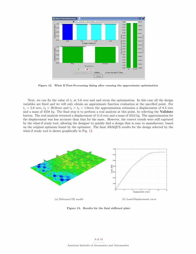
Figure 12. What If Post-Processing dialog after running the approximate optimization

Next, we can fix the value of t1 at 5.0 mm and and rerun the optimization. In this case all the designvariables are fixed and we will only obtain an approximate function evaluation at the specified point. Fort1 = 5.0 mm, t2 = 20.0mm and t3 = t4 = 1.0mm the approximation estimates a displacement of 8.3 mmand a mass of 4558 kg. The final step is to perform a real analysis at this point, by selecting the Validatebutton. The real analysis returned a displacement of 11.6 mm and a mass of 4513 kg. The approximation forthe displacement was less accurate than that for the mass.. However, the correct trends were still capturedby the what-if study tool, allowing the designer to quickly find a design that is easy to manufacture, basedon the original optimum found by the optimizer. The final ABAQUS results for the design selected by thewhat-if study tool is shown graphically in Fig. 13.

(a) Deformed FE model

0 2 4 6 8 10 120

1000

2000

3000

4000

5000

6000

7000

Displacement [mm]

Load

[kN

]

(b) Load-Displacement curve

Figure 13. Results for the final stiffened plate

9 of 10

American Institute of Aeronautics and Astronautics

V. Concluding Remarks

A new, interactive post-processing capability is introduced as part of VisualDOC Version 4.0. Thiscapability allows the user to interactively perform real-time what-if studies, based on optimization results.This is especially powerful if the analysis takes a long time. The tool allows the user to estimate the influenceof changing the optimization problem in real-time, before committing to a time-consuming optimization. Thetool also provides the user with a better feel and more insight into the optimization problem and addressesboth the issues of ease of use and high computational cost.

References

1VisualDOC Design Optimization Software, Version 4.x, Getting Started Manual, Vanderplaats Research and Develop-ment, Inc., 1767 S. 8th St., Colorado Springs, CO, 2004.

2DOT. Design Optimization Tools, Version 5.x, Users Manual , Vanderplaats Research and Development, Inc., 1767 S.8th St., Colorado Springs, CO, January 2001.

3Venter, G. and Sobieszczanski-Sobieski, J., “Particle Swarm Optimization,” Proceedings of the 43rdAIAA/ASME/ASCE/AHS/ASC Structures, Structural Dynamics, and Materials Conference, Denver, CO, AIAA-2002-1235,April 22–25 2002.

4Venter, G. and Sobieszczanski-Sobieski, J., “Multidisciplinary Optimization of a Transport Aircraft Wing using ParticleSwarm Optimization,” Proceedings of the 9th AIAA/ISSMO Symposium on Multidisciplinary Analysis and Optimization,Atlanta, GA, AIAA-2002-5644, September 4–6 2002.

5ABAQUS Example Problems Manual, Version 6.4-3 , ABAQUS, Inc., 1080 Main Street, Pawtucket, RI, 2004.

10 of 10

American Institute of Aeronautics and Astronautics