Polygonal finite elements for incompressible fluid flow · POLYGONAL FINITE ELEMENTS FOR...
18
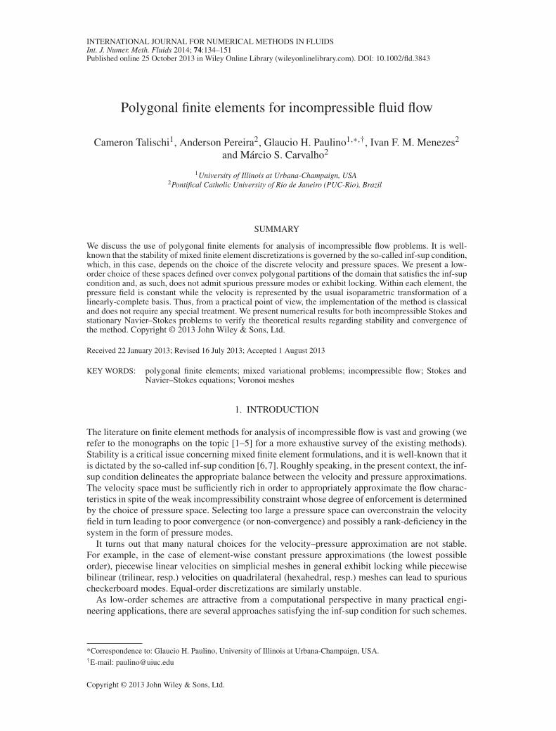
INTERNATIONAL JOURNAL FOR NUMERICAL METHODS IN FLUIDS Int. J. Numer. Meth. Fluids 2014; 74:134–151 Published online 25 October 2013 in Wiley Online Library (wileyonlinelibrary.com). DOI: 10.1002/fld.3843 Polygonal finite elements for incompressible fluid flow Cameron Talischi 1 , Anderson Pereira 2 , Glaucio H. Paulino 1, * ,† , Ivan F. M. Menezes 2 and Márcio S. Carvalho 2 1 University of Illinois at Urbana-Champaign, USA 2 Pontifical Catholic University of Rio de Janeiro (PUC-Rio), Brazil SUMMARY We discuss the use of polygonal finite elements for analysis of incompressible flow problems. It is well- known that the stability of mixed finite element discretizations is governed by the so-called inf-sup condition, which, in this case, depends on the choice of the discrete velocity and pressure spaces. We present a low- order choice of these spaces defined over convex polygonal partitions of the domain that satisfies the inf-sup condition and, as such, does not admit spurious pressure modes or exhibit locking. Within each element, the pressure field is constant while the velocity is represented by the usual isoparametric transformation of a linearly-complete basis. Thus, from a practical point of view, the implementation of the method is classical and does not require any special treatment. We present numerical results for both incompressible Stokes and stationary Navier–Stokes problems to verify the theoretical results regarding stability and convergence of the method. Copyright © 2013 John Wiley & Sons, Ltd. Received 22 January 2013; Revised 16 July 2013; Accepted 1 August 2013 KEY WORDS: polygonal finite elements; mixed variational problems; incompressible flow; Stokes and Navier–Stokes equations; Voronoi meshes 1. INTRODUCTION The literature on finite element methods for analysis of incompressible flow is vast and growing (we refer to the monographs on the topic [1–5] for a more exhaustive survey of the existing methods). Stability is a critical issue concerning mixed finite element formulations, and it is well-known that it is dictated by the so-called inf-sup condition [6, 7]. Roughly speaking, in the present context, the inf- sup condition delineates the appropriate balance between the velocity and pressure approximations. The velocity space must be sufficiently rich in order to appropriately approximate the flow charac- teristics in spite of the weak incompressibility constraint whose degree of enforcement is determined by the choice of pressure space. Selecting too large a pressure space can overconstrain the velocity field in turn leading to poor convergence (or non-convergence) and possibly a rank-deficiency in the system in the form of pressure modes. It turns out that many natural choices for the velocity–pressure approximation are not stable. For example, in the case of element-wise constant pressure approximations (the lowest possible order), piecewise linear velocities on simplicial meshes in general exhibit locking while piecewise bilinear (trilinear, resp.) velocities on quadrilateral (hexahedral, resp.) meshes can lead to spurious checkerboard modes. Equal-order discretizations are similarly unstable. As low-order schemes are attractive from a computational perspective in many practical engi- neering applications, there are several approaches satisfying the inf-sup condition for such schemes. *Correspondence to: Glaucio H. Paulino, University of Illinois at Urbana-Champaign, USA. † E-mail: [email protected] Copyright © 2013 John Wiley & Sons, Ltd.
Transcript of Polygonal finite elements for incompressible fluid flow · POLYGONAL FINITE ELEMENTS FOR...
INTERNATIONAL JOURNAL FOR NUMERICAL METHODS IN FLUIDSInt. J. Numer. Meth. Fluids 2014; 74:134–151Published online 25 October 2013 in Wiley Online Library (wileyonlinelibrary.com). DOI: 10.1002/fld.3843
Polygonal finite elements for incompressible fluid flow
Cameron Talischi1, Anderson Pereira2, Glaucio H. Paulino1,*,†, Ivan F. M. Menezes2
and Márcio S. Carvalho2
1University of Illinois at Urbana-Champaign, USA2Pontifical Catholic University of Rio de Janeiro (PUC-Rio), Brazil
SUMMARY
We discuss the use of polygonal finite elements for analysis of incompressible flow problems. It is well-known that the stability of mixed finite element discretizations is governed by the so-called inf-sup condition,which, in this case, depends on the choice of the discrete velocity and pressure spaces. We present a low-order choice of these spaces defined over convex polygonal partitions of the domain that satisfies the inf-supcondition and, as such, does not admit spurious pressure modes or exhibit locking. Within each element, thepressure field is constant while the velocity is represented by the usual isoparametric transformation of alinearly-complete basis. Thus, from a practical point of view, the implementation of the method is classicaland does not require any special treatment. We present numerical results for both incompressible Stokes andstationary Navier–Stokes problems to verify the theoretical results regarding stability and convergence ofthe method. Copyright © 2013 John Wiley & Sons, Ltd.
Received 22 January 2013; Revised 16 July 2013; Accepted 1 August 2013
KEY WORDS: polygonal finite elements; mixed variational problems; incompressible flow; Stokes andNavier–Stokes equations; Voronoi meshes
1. INTRODUCTION
The literature on finite element methods for analysis of incompressible flow is vast and growing (werefer to the monographs on the topic [1–5] for a more exhaustive survey of the existing methods).Stability is a critical issue concerning mixed finite element formulations, and it is well-known that itis dictated by the so-called inf-sup condition [6,7]. Roughly speaking, in the present context, the inf-sup condition delineates the appropriate balance between the velocity and pressure approximations.The velocity space must be sufficiently rich in order to appropriately approximate the flow charac-teristics in spite of the weak incompressibility constraint whose degree of enforcement is determinedby the choice of pressure space. Selecting too large a pressure space can overconstrain the velocityfield in turn leading to poor convergence (or non-convergence) and possibly a rank-deficiency in thesystem in the form of pressure modes.
It turns out that many natural choices for the velocity–pressure approximation are not stable.For example, in the case of element-wise constant pressure approximations (the lowest possibleorder), piecewise linear velocities on simplicial meshes in general exhibit locking while piecewisebilinear (trilinear, resp.) velocities on quadrilateral (hexahedral, resp.) meshes can lead to spuriouscheckerboard modes. Equal-order discretizations are similarly unstable.
As low-order schemes are attractive from a computational perspective in many practical engi-neering applications, there are several approaches satisfying the inf-sup condition for such schemes.
*Correspondence to: Glaucio H. Paulino, University of Illinois at Urbana-Champaign, USA.†E-mail: [email protected]
Copyright © 2013 John Wiley & Sons, Ltd.

POLYGONAL FINITE ELEMENTS FOR INCOMPRESSIBLE FLUID FLOW 135
For example, one approach is to introduce enrichments to the velocity space in the form of inter-nal or edge bubble functions. A well-known example is the MINI element of Arnold et al. [8].Stabilization methods that introduce residual or penalty terms to augment the variational statementof the problem have also been successfully applied to obtain stable low-order formulations ‡ (see,for example, [9–11]). However, mesh-dependent parameters in such formulations must be chosencarefully, and special data structures may be needed for the numerical implementation [12]. In thisregard, we mention the recent work [13], based on local projection operators, which addresses theaforementioned shortcomings. Finally, certain mesh topologies have been shown to be stable evenwhen the underlying spaces are in general not inf-sup compatible. One example is the macroelementmesh in [14], which consists of a special arrangement of quadrilaterals. Another related approach isdue to Hauret et al. [15] where ‘diamond’ meshes are constructed from simplicial partitions of thedomain and the choice of spaces together with the special structure of the mesh ensure stability.
As illustrated in this paper, low-order velocity and pressure approximations based on a largeclass of polygonal discretizations satisfy the inf-sup condition without the need for any additionaltreatment. Intuitively, this stability can be attributed to the presence of more velocity DOFs forpolygonal elements with many sides (per pressure DOF) when compared to triangular and quadri-lateral discretizations. We remark that we have observed similar characteristics of polygonal dis-cretizations in topology optimization [16–19] where spurious checkerboard-like patterns also plaguetriangular and quadrilateral discretizations [20].
While the development of polygonal finite elements has had a long history, dating back to the sem-inal work of Wachspress [21], their numerical implementation and application to solving PDEs ismore recent (see, for example, [22–25]). From a practical perspective, the greater flexibility for meshgeneration is an attractive feature of polygonal finite elements. On the one hand, local modificationsof the mesh (e.g., refinement through element splitting used in [26]) is made possible by the factthat not all the elements have to be topologically equivalent. On the other hand, a number of meshgeneration algorithms, harnessing the properties of Voronoi diagrams, have been developed recently[27–30]. In addition to advantages in mesh generation, polygonal finite elements can outperformtheir triangular and quadrilateral counterparts in terms of accuracy (see the example in section 3.2of [17] where the overall system size can be smaller for a given level of error).
Recently, a number of mimetic finite difference (MFD) schemes have been developed for solvingPDEs on polygonal and polyhedral meshes. While some MFD formulations (e.g., [31]) are closelyrelated to mixed finite elements, purely nodal MFD schemes (e.g., [32, 33]) are related to primalfinite elements. This connection is elucidated in the recent work [34] wherein an FEM-like incarna-tion of MFD, labeled Virtual Element Method, is developed. Of particular relevance to the presentwork are the MFD formulations for incompressible Stokes flow for polygonal meshes reported in[35, 36]. While the formulation in [35] features edge DOFs for the velocity field, the results in [36]delineate the conditions on the mesh topology under which nodal velocity DOFs are sufficient toensure stability. For meshes consisting of convex elements, one such scenario is when each interiornode is incident to at most three edges. This property naturally excludes triangular and quadrilat-eral grids and requires the elements to have many sides. Even though in the mimetic frameworkan explicit construction of the basis functions is not needed, the present finite element scheme is arealization of the MFD formulation considered in [36]. Thus, as we will show later in Section 5, theresults of [36] are applicable to our formulation.
The remainder of this paper is organized as follows: in the next section, we introduce the problemof incompressible Stokes flow, which serves as the model problem for the theoretical discussion.In Section 3, we present the mixed variational finite element discretization of the problem and dis-cuss sufficient conditions for convergence. Next, in Section 4, we show the construction of thelow-order velocity and pressure space for convex polygonal meshes. The specific condition on themesh topology that is sufficient for stability is discussed and verified in Section 5. Numerical resultsdemonstrating convergence of the method for both Stokes and stationary Navier–Stokes problemsare provided in Section 6. We conclude the paper with some remarks in Section 7.
‡In some instances, one can establish an equivalence between enrichment and stabilized methods (see, for example [37]).
Copyright © 2013 John Wiley & Sons, Ltd. Int. J. Numer. Meth. Fluids 2014; 74:134–151DOI: 10.1002/fld
136 C. TALISCHI ET AL.
We briefly and partially introduce the notation adopted in this paper. We denote by H k.�/ thestandard Sobolev space consisting of functions whose derivatives up to the kth order are square-integrable over the given domain � and write k�kk for its norm. We write L2.�/ D H 0.�/ anddenote by H 1
0 .�/ functions in H 1.�/ that vanish on the boundary @�. For any subset E � �,we denote by jEj its measure and by �E its characteristic (or indicator) function. This means that�E .x/ D 1 if x 2 E and �E .x/ D 0 if x 2 �nE. The interior of E is denoted by int.E/ and itsclosure by E.
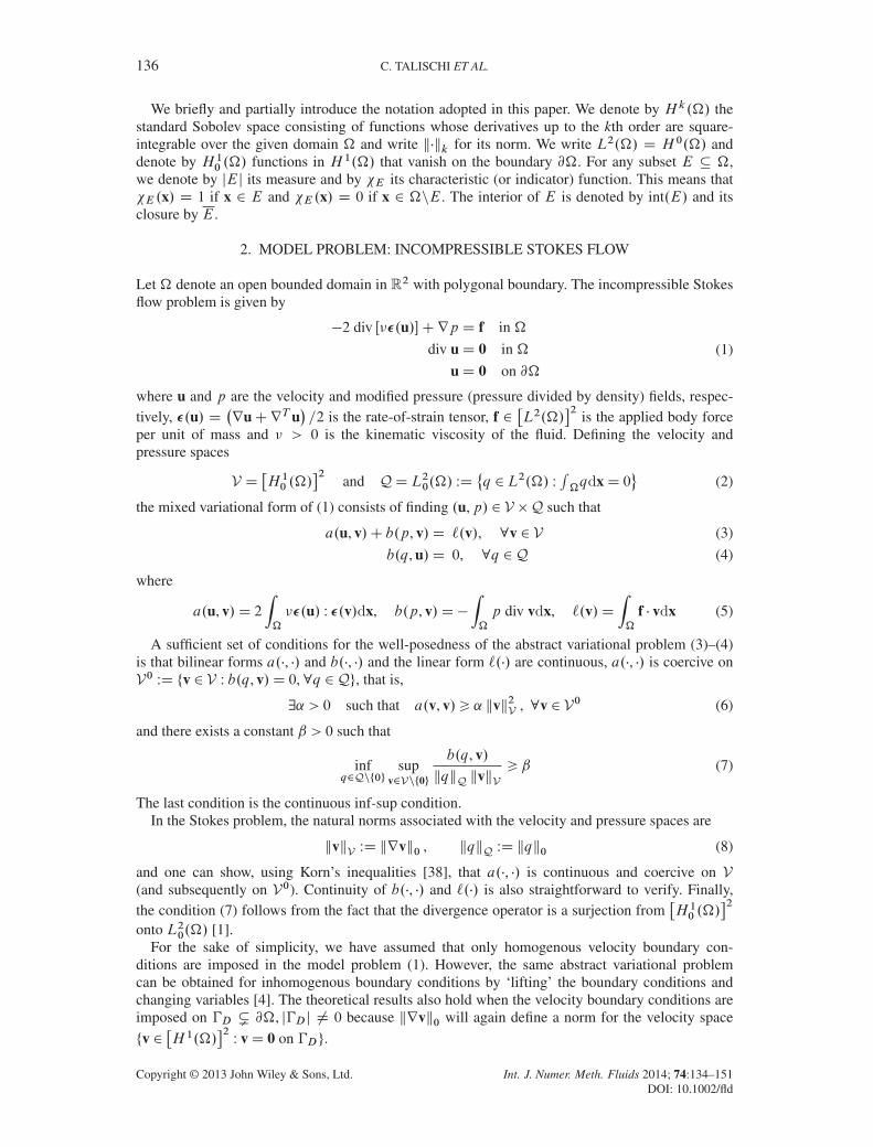
2. MODEL PROBLEM: INCOMPRESSIBLE STOKES FLOW
Let � denote an open bounded domain in R2 with polygonal boundary. The incompressible Stokesflow problem is given by
�2 div Œ��.u/�Crp D f in �
div uD 0 in �
uD 0 on @�
(1)
where u and p are the velocity and modified pressure (pressure divided by density) fields, respec-tively, �.u/ D
�ruCrT u
�=2 is the rate-of-strain tensor, f 2
�L2.�/
�2is the applied body force
per unit of mass and � > 0 is the kinematic viscosity of the fluid. Defining the velocity andpressure spaces
V D�H 10 .�/
�2and QD L20.�/ WD
®q 2 L2.�/ W
R�qdxD 0
¯(2)
the mixed variational form of (1) consists of finding .u,p/ 2 V �Q such that
a.u, v/C b.p, v/D `.v/, 8v 2 V (3)
b.q, u/D 0, 8q 2Q (4)
where
a.u, v/D 2Z�
��.u/ W �.v/dx, b.p, v/D�Z�
p div vdx, `.v/DZ�
f � vdx (5)
A sufficient set of conditions for the well-posedness of the abstract variational problem (3)–(4)is that bilinear forms a.�, �/ and b.�, �/ and the linear form `.�/ are continuous, a.�, �/ is coercive onV0 WD ¹v 2 V W b.q, v/D 0,8q 2Qº, that is,
9˛ > 0 such that a.v, v/> ˛ kvk2V , 8v 2 V0 (6)
and there exists a constant ˇ > 0 such that
infq2Qn¹0º
supv2Vn¹0º
b.q, v/kqkQ kvkV
> ˇ (7)
The last condition is the continuous inf-sup condition.In the Stokes problem, the natural norms associated with the velocity and pressure spaces are
kvkV WD krvk0 , kqkQ WD kqk0 (8)
and one can show, using Korn’s inequalities [38], that a.�, �/ is continuous and coercive on V(and subsequently on V0). Continuity of b.�, �/ and `.�/ is also straightforward to verify. Finally,the condition (7) follows from the fact that the divergence operator is a surjection from
�H 10 .�/
�2onto L20.�/ [1].
For the sake of simplicity, we have assumed that only homogenous velocity boundary con-ditions are imposed in the model problem (1). However, the same abstract variational problemcan be obtained for inhomogenous boundary conditions by ‘lifting’ the boundary conditions andchanging variables [4]. The theoretical results also hold when the velocity boundary conditions areimposed on �D ¨ @�, j�Dj ¤ 0 because krvk0 will again define a norm for the velocity space
¹v 2�H 1.�/
�2W vD 0 on �Dº.
Copyright © 2013 John Wiley & Sons, Ltd. Int. J. Numer. Meth. Fluids 2014; 74:134–151DOI: 10.1002/fld

POLYGONAL FINITE ELEMENTS FOR INCOMPRESSIBLE FLUID FLOW 137
3. FINITE ELEMENT APPROXIMATION
Considering the finite element subspaces Vh � V and Qh � Q, with h indicating the maximumdiameter of elements in the underlying mesh, the Galerkin approximation of (3)–(4) consists ofseeking .uh,ph/ 2 Vh �Qh such that
a.uh, vh/C b.ph, vh/D `.vh/, 8vh 2 Vh (9)
b.qh, uh/D 0, 8qh 2Qh (10)
The approximate problem (9)–(10) is well-posed if, in addition to the previously stated continuityand coercivity requirements,
ˇh WD infqh2Qhn¹0º
supvh2Vhn¹0º
b.qh, vh/kqhkQ kvhkV
> 0 (11)
This is nothing but the discrete version of the inf-sup condition (7) and is sometimes referred toas the Ladyzenskaja-Babuska-Brezzi or LBB condition [6, 7]. Observe that for the Stokes prob-lem, a.�, �/ is coercive on all of V , and so it follows that it is also coercive on the subspaceV0hWD ¹vh 2 Vh W b.qh, vh/D 0,8q 2Qhº §.
Moreover, under these conditions, the finite element solution pair .uh,ph/ satisfies the followingerror estimates [4]:
ku� uhkV 6�1C
ca
˛
��1C
cb
ˇh
inf
vh2Vhku� vhkV C
cb
˛inf
qh2Qhkp � qhkQ (12)
kp � phkQ 6ca
ˇh
�1C
ca
˛
��1C
cb
ˇh
inf
vh2Vhku� vhkV
C
�1C
cb
ˇhCcacb
˛ˇh
inf
qh2Qhkp � qhkQ (13)
for some positive constants ca and cb ¶.With the typical choice of finite element spaces, standard interpolation error estimates show that
the distances infvh2Vh kv� vhkV and infqh2Qh kp � qhkQ vanish under mesh refinement as h! 0.The estimates (12)–(13) then prove convergence of the finite element solutions provided that ˇhremains bounded away from zero. More specifically, if ˇh > ˇ0 for some fixed constant ˇ0 > 0 andall h, then the distance between .u,p/ and .uh,ph/ is on the order of the distance between .u,p/and its best approximation in Vh � Qh, and the method achieves an optimal rate of convergence.Otherwise, if ˇh ! 0 with h, the finite element formulation is said to exhibit locking. Intuitively,locking occurs when, given a finite element pressure space Qh, the velocity space Vh is not suf-ficiently rich to both satisfy the weak incompressibility constraint (4) and approximate the flowcharacteristics. Mesh refinement does not alleviate the problem because it also enriches the pressurespace Qh. Therefore, it is important to recognize that preventing locking involves the appropriateselection of Vh with respect to the given choice of pressure discretization.
Aside from locking, the other important issue related to stability of the mixed finite element for-mulations is the appearance of spurious modes. The pair of spaces Vh and Qh admits a spuriouspressure mode if there exists Qph 2Qhn¹0º such that
b . Qph, vh/D 0 8vh 2 Vh (14)
§In general, coercivity of a.�, �/ on V0 does not imply its coercivity on V0h because we may have V0h ª V0. In such cases,the latter must be verified independently for the given spaces Vh and Qh.
¶These constants are in fact the norms associated with the bilinear forms a.�, �/ and b.�, �/. Notice that in these estimates,we have used the fact that a.�, �/ is ˛-coercive on V0h (see the remark in the previous footnote).
Copyright © 2013 John Wiley & Sons, Ltd. Int. J. Numer. Meth. Fluids 2014; 74:134–151DOI: 10.1002/fld

138 C. TALISCHI ET AL.
If pressure modes are present, then the discrete inf-sup condition (11) cannot be satisfied (the sta-bility constant ˇh is simply zero), and so the finite element problem is not well-posed. Observe thatif .uh,ph/ is the solution to (9)–(10), then .uh,ph C s Qph/ is also a solution for any s 2 R anda spurious pressure mode Qph. Conversely, for finite-dimensional spaces Vh and Qh, the violationof the discrete inf-sup condition implies existence of spurious modes. We note that the appearanceof pressure modes is problem-dependent (for the same velocity–pressure pair, the pressure modemay or may not exist depending on the boundary conditions of the problem) while locking is moreintrinsic to the degree of interpolation of velocity and pressure fields.
We conclude this brief discussion by noting that there exists certain improved error estimates,most notably for the bilinear-velocity constant-pressure element, which show that the approximatevelocity solution in some cases can be accurate, despite the failure to satisfy the inf-sup condition[2,39–42]. However, such elements can be unreliable in general and should be used only by knowl-edgable practitioners. For example, the presence of spurious modes can lead to an ill-posed discreteproblem (one with no solutions) when certain inhomogenous boundary conditions are prescribed(see, for example, [43, 44]).
4. VELOCITY AND PRESSURE SPACES ON POLYGONAL DISCRETIZATIONS
In this section, we define a low-order pair of velocity and pressure spaces defined on polygonalmeshes that leads to a stable finite element approximation. Consider a mesh Th D ¹�mºMmD1 con-sisting of closed strictly convex polygons that form a partition of the domain � ||. The mesh size his the maximum diameter of the elements in Th. Aside from the usual shape-regularity assumptions,we must require certain conditions of the topology of Th in order to ensure the satisfaction of theinf-sup condition. These will be discussed in the next section.
We define the discrete pressure space Qh to simply consist of element-wise constant functions onTh, that is
Qh D®qh 2 L
20.�/ W qhj�m D constant, 8mD 1, : : : ,M
¯(15)
This is, in some sense, the lowest possible order discretization for the pressure field. Observe thateach admissible pressure function qh 2Qh has the form
qh D
MXmD1
cm��m (16)
where cm is the constant value of qh over themth element (recall that ��m � 1 on�m and vanisheselsewhere). However, because
R� qhdxD 0, the coefficients must satisfy the following relation:
MXmD1
cm j�mj D 0 (17)
In order to enforce the zero-mean condition, we consider the following set of pressure basisfunctions
m WD ��m �j�mj
j�M j��M , mD 1, : : : ,M � 1 (18)
Observe that Qh D span ¹ 1, : : : , M�1º and that themth DOF, for 16m6M �1, corresponds tothe pressure in �m (we refer the reader to [45] for a more general discussion of such construction).Using the standard finite element approximation theory, we can show that for p 2H�.�/\Q, with0 < �6 1, we have infqh2Qh kp � qhkQ DO.h�/.
||Therefore,[MmD1�m D� and int .�m/\ int .�m0/D; ifm¤m0. By strictly convex, we mean that no three verticesof the polygon are collinear.
Copyright © 2013 John Wiley & Sons, Ltd. Int. J. Numer. Meth. Fluids 2014; 74:134–151DOI: 10.1002/fld
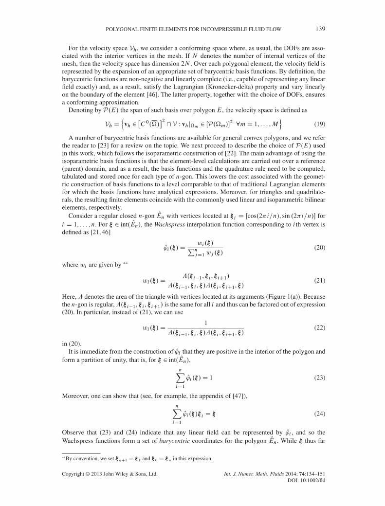
POLYGONAL FINITE ELEMENTS FOR INCOMPRESSIBLE FLUID FLOW 139
For the velocity space Vh, we consider a conforming space where, as usual, the DOFs are asso-ciated with the interior vertices in the mesh. If N denotes the number of internal vertices of themesh, then the velocity space has dimension 2N . Over each polygonal element, the velocity field isrepresented by the expansion of an appropriate set of barycentric basis functions. By definition, thebarycentric functions are non-negative and linearly complete (i.e., capable of representing any linearfield exactly) and, as a result, satisfy the Lagrangian (Kronecker-delta) property and vary linearlyon the boundary of the element [46]. The latter property, together with the choice of DOFs, ensuresa conforming approximation.
Denoting by P.E/ the span of such basis over polygon E, the velocity space is defined as
Vh D°
vh 2�C 0.�/
�2\ V W vhj�m 2 ŒP.�m/�2 8mD 1, : : : ,M
±(19)
A number of barycentric basis functions are available for general convex polygons, and we referthe reader to [23] for a review on the topic. We next proceed to describe the choice of P.E/ usedin this work, which follows the isoparametric construction of [22]. The main advantage of using theisoparametric basis functions is that the element-level calculations are carried out over a reference(parent) domain, and as a result, the basis functions and the quadrature rule need to be computed,tabulated and stored once for each type of n-gon. This lowers the cost associated with the geomet-ric construction of basis functions to a level comparable to that of traditional Lagrangian elementsfor which the basis functions have analytical expressions. Moreover, for triangles and quadrilate-rals, the resulting finite elements coincide with the commonly used linear and isoparametric bilinearelements, respectively.
Consider a regular closed n-gon OEn with vertices located at �i D Œcos.2�i=n/, sin .2�i=n/� fori D 1, : : : ,n. For � 2 int. OEn/, the Wachspress interpolation function corresponding to i th vertex isdefined as [21, 46]
O'i .�/Dwi .�/PnjD1wj .�/
(20)
where wi are given by **
wi .�/DA.�i�1, �i , �iC1/
A.�i�1, �i , �/A.�i , �iC1, �/(21)
Here, A denotes the area of the triangle with vertices located at its arguments (Figure 1(a)). Becausethe n-gon is regular,A.�i�1, �i , �iC1/ is the same for all i and thus can be factored out of expression(20). In particular, instead of (21), we can use
wi .�/D1
A.�i�1, �i , �/A.�i , �iC1, �/(22)
in (20).It is immediate from the construction of O'i that they are positive in the interior of the polygon and
form a partition of unity, that is, for � 2 int. OEn/,
nXiD1
O'i .�/D 1 (23)
Moreover, one can show that (see, for example, the appendix of [47]),
nXiD1
O'i .�/�i D � (24)
Observe that (23) and (24) indicate that any linear field can be represented by O'i , and so theWachspress functions form a set of barycentric coordinates for the polygon OEn. While � thus far
**By convention, we set �nC1 D �1 and �0 D �n in this expression.
Copyright © 2013 John Wiley & Sons, Ltd. Int. J. Numer. Meth. Fluids 2014; 74:134–151DOI: 10.1002/fld
140 C. TALISCHI ET AL.
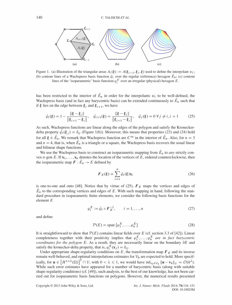
Figure 1. (a) Illustration of the triangular areas Ai .�/ WD A.�i�1, �i , �/ used to define the interpolant wi ;(b) contour lines of a Wachspress basis function O'i over the regular (reference) hexagon OE6; (c) contour
lines of the ‘isoparametric’ basis function 'Ei
over an irregular (physical) hexagon E.
has been restricted to the interior of OEn in order for the interpolants wi to be well-defined, theWachspress basis (and in fact any barycentric basis) can be extended continuously to OEn such thatif � lies on the edge between �i and �iC1, we have
O'i .�/D 1�k� � �ik�iC1 � �i , O'iC1.�/D
k� � �ik�iC1 � �i , O'j .�/D 0 8j ¤ i , i C 1 (25)
As such, Wachspress functions are linear along the edges of the polygon and satisfy the Kronecker-delta property O'i .�j / D ıij (Figure 1(b)). Moreover, this means that properties (23) and (24) hold
for all � 2 OEn. We remark that Wachspress function are C1 in the interior of OEn. Also, for n D 3and nD 4, that is, when OEn is a triangle or a square, the Wachspress basis recovers the usual linearand bilinear shape functions.
We use the Wachspress basis to construct an isoparametric mapping from OEn to any strictly con-vex n-gon E. If x1, : : : , xn denotes the location of the vertices of E, ordered counterclockwise, thenthe isoparametric map F W OEn!E defined by
F E .�/D
nXiD1
O'i .�/xi (26)
is one-to-one and onto [48]. Notice that by virtue of (25), F E maps the vertices and edges ofOEn to the corresponding vertices and edges of E. With such mapping in hand, following the stan-
dard procedure in isoparametric finite elements, we consider the following basis functions for theelement E
'Ei WD O'i ıF�1E , i D 1, : : : ,n (27)
and define
P.E/D span®'E1 , : : : ,'En
¯(28)
It is straightforward to show that P.E/ contains linear fields over E (cf. section 3.3 of [42]). Linearcompleteness together with their positivity implies that 'E1 , : : : ,'En are in fact barycentriccoordinates for the polygon E. As a result, they are necessarily linear on the boundary @E andsatisfy the kronecker-delta property, that is, 'Ei .xj /D ıij .
Under appropriate shape-regularity conditions on E, the transformation map F E and its inverseremain well-behaved, and optimal interpolations estimates for Vh are expected to hold. More specif-
ically, for u 2�H 1C�.�/
�2\ V , with 0 < � 6 1, we would have infvh2Vh ku� vhkV D O.h�/.
While such error estimates have appeared for a number of barycentric basis (along with suitableshape-regularity conditions) (cf. [49]), such analysis, to the best of our knowledge, has not been car-ried out for isoparametric basis functions on polygons. However, the numerical results presented
Copyright © 2013 John Wiley & Sons, Ltd. Int. J. Numer. Meth. Fluids 2014; 74:134–151DOI: 10.1002/fld

POLYGONAL FINITE ELEMENTS FOR INCOMPRESSIBLE FLUID FLOW 141
Figure 2. Illustration of the integration scheme using ‘quadrangulation’ of the polygon (a) integration pointsusing 2� 2 Gauss quadrature for each cell of the reference hexagon; (b) location of the integration points inthe physical element; (c) location of integration points in the physical element for the ‘triangulation’ scheme.
in the next section confirm this conjecture. Note that the choice of spaces Vh and Qh is opti-mal in that both terms in the approximation errors (12)–(13) are O.h/ when the exact solution issufficiently smooth.
We close this section by discussing the quadrature scheme used for evaluating the weak formintegrals. For n D 3 and n D 4, we use the standard quadrature rules for triangles and quads, andfor n > 5, we divide OEn into n quadrilaterals (by connecting the centroid to the midpoint of eachedge) and use the well-known Gauss quadrature rules on each quadrilateral (cf. Figure 2). We havefound that this scheme provides better accuracy compared to the triangulation approach adopted in[17,22]. We should also note that a number of specific quadrature rules for polygonal domains haverecently appeared [50,51], although, for the purposes of this work, the adopted scheme is sufficient.
Finally, we observe that with the present choice of velocity and pressure spaces, the bilinear formb.�, �/ can be evaluated exactly (this fact is also noted and used in [36]). Indeed, for any qh 2 Qhand vh 2 Vh,
b.qh, vh/D�MXmD1
qhj�m
Z�m
div vhdxD�MXmD1
qhj�m
Z@�m
vh � nds (29)
where we have used the fact that qh is element-wise constant. Because vh varies linearly over @�m,the last integral can be computed using the nodal values of vh. In fact, the particular construction ofbarycentric basis functions over�m is immaterial for the bilinear form b.�, �/ because all barycentricbasis functions are linear on the boundary.
5. STABILITY AND SATISFACTION OF THE INF-SUP CONDITION
Without additional restrictions on the family of meshes Th, the pair of discrete spaces Vh and Qhdefined in the previous section does not necessarily satisfy the inf-sup condition. So far, we havenot yet excluded the cases where Th is a triangular or quadrilateral mesh.
In [36], a set of conditions on the topology of Th that guarantees the satisfaction of the inf-supcondition for the choice of velocity and pressures defined here is identified. Although the originalproof by Beirão Da Veiga and Lipnikov is given in the context of MFD, the results are applicableto the present setting because the pressure spaces are identical and Vh is one particular realizationof the velocity space considered in [36] when no bubble DOFs are present. Furthermore, in light ofequation (29) in the previous section and equations (6) and (9) in [36], the definition of bilinear formb.�, �/ is also identical. In fact, the main difference between the two formulations is the treatment ofbilinear form a.�, �/.
As mentioned in the introduction, for meshes consisting of convex polygons, their result guaran-tees the satisfaction of inf-sup condition if every internal node/vertex in the mesh is connected to atmost three edges. This, for example, holds for meshes obtained from a Voronoi tessellation of thedomain where no four neighboring seeds lie on a circle and thus each internal vertex is incident to
Copyright © 2013 John Wiley & Sons, Ltd. Int. J. Numer. Meth. Fluids 2014; 74:134–151DOI: 10.1002/fld
142 C. TALISCHI ET AL.
exactly three edges. By contrast, a structured grid of rectangular elements violates it because theinternal vertices are connected to four edges.
In practice, such convex polygonal meshes can be constructed using an appropriate Voronoi-basedmeshing algorithm [27, 28, 52]. While it is possible that the Voronoi tessellation of a non-convexdomain from an arbitrary set of seeds contains non-convex elements near the boundary, the approachproposed in [27, 28, 52] avoids this by including additional seeds, obtained from reflections of theinterior seeds about the boundary, and considering the Voronoi tessellation of the entire plane. Asuitable mesh is given by a subset of this Voronoi diagram, which necessarily consists only ofconvex elements. In [28], the regularity of the mesh is ensured by requiring that the Voronoi dia-gram is centroidal (that is, the centroid of each element coincides with the generating seed). Wewill show numerical results for both random Voronoi and centroidal Voronoi (CVT) meshes inthis paper.
We validate the applicability of the previous condition in the present setting by computing thestability parameter ˇh for different families of meshes and a sequence of progressively finer meshesfor each family. While this ‘test’ only furnishes a necessary condition for satisfaction of the inf-supcondition, it is shown in [53] to reliably correlate with the known theoretical results. In the fol-lowing, we briefly discuss the procedure for the calculation of the stability parameter following theapproach of [53].
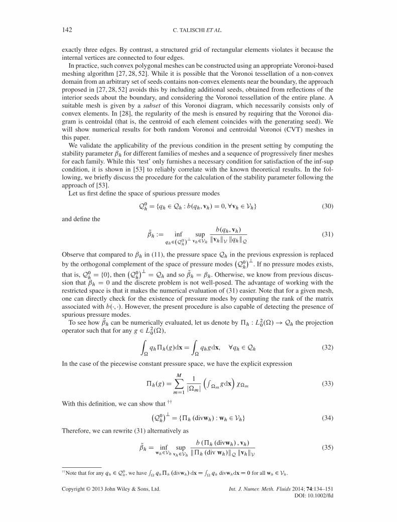
Let us first define the space of spurious pressure modes
Q0h D ¹qh 2Qh W b.qh, vh/D 0,8vh 2 Vhº (30)
and define the
Q̌h WD inf
qh2.Q0h/?
supvh2Vh
b.qh, vh/kvhkV kqhkQ
(31)
Observe that compared to ˇh in (11), the pressure space Qh in the previous expression is replaced
by the orthogonal complement of the space of pressure modes�Q0h
�?. If no pressure modes exists,
that is, Q0hD ¹0º, then
�Q0h
�?D Qh and so Q̌h D ˇh. Otherwise, we know from previous discus-
sion that ˇh D 0 and the discrete problem is not well-posed. The advantage of working with therestricted space is that it makes the numerical evaluation of (31) easier. Note that for a given mesh,one can directly check for the existence of pressure modes by computing the rank of the matrixassociated with b.�, �/. However, the present procedure is also capable of detecting the presence ofspurious pressure modes.
To see how Q̌h can be numerically evaluated, let us denote by …h W L20.�/! Qh the projection
operator such that for any g 2 L20.�/,Z�
qh…h.g/dxDZ�
qhgdx, 8qh 2Qh (32)
In the case of the piecewise constant pressure space, we have the explicit expression
…h.g/D
MXmD1
1
j�mj
�R�mgdx
���m (33)
With this definition, we can show that ††
�Q0h�?D ¹…h .divwh/ W wh 2 Vhº (34)
Therefore, we can rewrite (31) alternatively as
Q̌h D inf
wh2Vhsup
vh2Vh
b .…h .divwh/ , vh/k…h .div wh/kQ kvhkV
(35)
††Note that for any qh 2Q0h, we have
R�qh…h .divwh/dxD
R�qh divwhdxD 0 for all wh 2 Vh.
Copyright © 2013 John Wiley & Sons, Ltd. Int. J. Numer. Meth. Fluids 2014; 74:134–151DOI: 10.1002/fld

POLYGONAL FINITE ELEMENTS FOR INCOMPRESSIBLE FLUID FLOW 143
Figure 3. Representative example of the family of meshes: (a) uniform quadrilateral, (b) uniform hexagonal,(c) random Voronoi and (d) centroidal Voronoi (CVT).
Moreover, from (32), we have
b .…h .div wh/ , vh/DZ�
…h .div wh/ div vhdxDZ�
…h .div wh/…h .div vh/dx (36)
which gives the symmetric expression
Q̌h D inf
wh2Vhsup
vh2Vh
R�…h .div wh/…h .div vh/dx
k…h .div wh/kQ kvhkV(37)
Let us denote by ¹'iº2NiD1 the set of basis functions for the velocity space Vh and define the following
matrices associated with the terms in (37):
ŒSh�ij DZ�
r'i W r'jdx, ŒGh�ij D
Z�
…h .div 'i /…h
�div 'j
�dx (38)
Observe that Sh is positive definite and Gh is positive semi-definite. We have the following relationfor Q̌h
Q̌h D inf
W2R2Nsup
V2R2N
WTGhV�WTGhW
�1=2 �VT ShV
�1=2 (39)
From this and after some algebra, one can show that [2, 53, 54]
Q̌h Dp� (40)
where � is the smallest nonzero eigenvalue for the following eigenvalue problem
GhVD �ShV (41)
The number of spurious pressure modes can also be obtained from the eigenvalue problem (41). Ifthere are k � 1 zero eigenvalues, then there are max .k � 2N CM � 1, 0/ pressure modes present,where N and M are the total number of nodes and elements, respectively. We note that Q̌h > 0 insuch a case even though ˇh D 0 and the inf-sup condition is not satisfied.
We consider four families of meshes over the unit square �D .0, 1/2, and as in the model prob-lem (1), the velocity boundary conditions are imposed on the entire boundary @�. A representativemesh for each family is shown in Figure 3. For each mesh type, the quantity Q̌h was computed onfive progressively finer meshes ‡‡, and the results are shown in Figure 4. For the bilinear quads, Q̌his evidently O.h/, consistent with the existing theory [5] and thus decays with mesh refinement.However, this quantity remains bounded away from zero for the three types of polygonal meshes.This is the case in spite of the fact that there are few occasions in the CVT meshes where an internaledge is connected to four edges (this is due to a procedure in the algorithm proposed in [28] thatcollapses very small edges in the mesh into a single vertex). Finally, while a checkerboard mode isdetected for every square grid, the polygonal meshes are free of any spurious pressure modes.
‡‡The mesh size is the maximum diameter of the elements in the mesh, that is, hDmaxm diam.�m/.
Copyright © 2013 John Wiley & Sons, Ltd. Int. J. Numer. Meth. Fluids 2014; 74:134–151DOI: 10.1002/fld

144 C. TALISCHI ET AL.
Figure 4. Computed values of the stability parameter Q̌h and mesh size h for different families of meshes.Note that the horizontal axis is in reverse (decreasing) order.
6. NUMERICAL STUDIES
In this section, we present a variety of numerical results confirming the stability and convergence ofpolygon finite elements and assess their performance for the families of meshes used in the previoussection.
First, we consider a Stokes flow problem on the unit square � D .0, 1/2 with known analyticalsolution given by §§
u1.x/D r.x1/ sin.ax2/, u2.x/D r 0.x1/ cos.ax2/=a, p.x/D x1x22 � 1=6 (42)
where r.x/ D .1 � x/ sin.ax/ and a D 2.2� . The velocity boundary conditions on @� as wellas the body force f are prescribed in accordance with (42) and � D 1. For polygonal elements, asecond-order quadrature rule, as illustrated in Figure 2(a and b), is used. We consider 10 randomly-generated meshes for each mesh level for the random Voronoi and CVT families. In addition to thepolygonal meshes, we also provide the results for uniform triangular meshes ¶¶ consisting of thestable MINI element [8] for the purposes of comparison.
We consider three measures for the error in the finite element solution given by
ku� uhk0 , ku� uhkV , kp � phkQ (43)
The convergence plots are shown in Figure 5 where, in the case of random Voronoi and CVT meshes,the figures show the average errors and the mesh sizes for each mesh level. The results indicate thatin every case, the solutions exhibit the optimal rates of convergence in the respective error norms.In fact, the L2-error in pressure converges at a faster rate than O.h/ for all the mesh families. Thisoptimal performance is even exhibited, on average, by the random Voronoi meshes despite the varia-tions in the meshes (we note, however, that the variations of error become smaller for finer meshes).Finally, we observe that the quadrilateral discretization, while not inf-sup stable, does provide con-vergent velocity solutions. The pressure field, however, contains spurious checkerboard modes inevery quadrilateral mesh.
As a way of comparing the performance of the different discretizations, we next plot theerror as a function of number of DOFs in Figure 6. While the number of DOFs indicates the size
§§This problem is proposed and solved in [36].¶¶The triangular meshes are obtained by splitting each element in the uniform quadrilateral grids along its left diagonal.
Copyright © 2013 John Wiley & Sons, Ltd. Int. J. Numer. Meth. Fluids 2014; 74:134–151DOI: 10.1002/fld

POLYGONAL FINITE ELEMENTS FOR INCOMPRESSIBLE FLUID FLOW 145
Figure 5. Plots of error versus mesh size for problem (42): (a) L2-error in velocity, (b)H1-error in velocityand (c) L2-error in pressure. Note that the horizontal axis is in reverse (decreasing) order.
Figure 6. Plots of error versus the number of DOFs for problem (42): (a) L2-error in velocity, (b) H1-errorin velocity and (c) L2-error in pressure.
of the associated discrete system, it is not a perfect measure for computational performance becauseit does not account for the cost of computing the element matrices and the structure of the linearsystem and its influence of the convergence of linear solver. Nevertheless, we observe several note-worthy facts from these plots. First, the CVT and hexagonal meshes, owing to their regularity,perform better than the random Voronoi meshes. While the velocity errors are comparable forCVT and hexagonal families, CVT meshes provide more accurate pressure solutions. Also, it isinteresting to note that all polygonal discretizations, including random Voronoi meshes, require asmaller number of DOFs for a given level of accuracy than the MINI discretization. The difference ispronounced for pressure solutions where, in the range of errors considered, the MINI discretizationrequires two orders of magnitude more DOFs than the CVT family. It is also interesting to notethat the quadrilateral meshes provide better performance for the calculation for the velocity field.This may be attributed to the fact that the exact velocity field for this problem is multiplicativelyseparable in x1 and x2 and is thus particularly well-suited for approximation by the tensor productin quadrilateral meshes.
We also examine the error in approximating the incompressibility of the velocity field. Figure 7shows plots of the L2-norm of div uh as a function of mesh size and number of DOFs. We can seethat the div uh converges to div u� 0 with a linear rate in h for all mesh families. The accuracy incapturing the incompressibility constraint, in terms of the total number of DOFs, is about the samefor quadrilateral, hexagonal and CVT meshes.
Copyright © 2013 John Wiley & Sons, Ltd. Int. J. Numer. Meth. Fluids 2014; 74:134–151DOI: 10.1002/fld
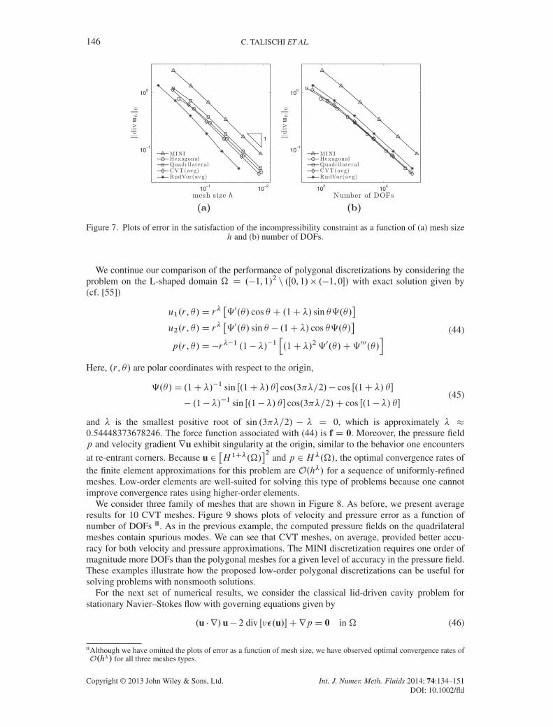
146 C. TALISCHI ET AL.
Figure 7. Plots of error in the satisfaction of the incompressibility constraint as a function of (a) mesh sizeh and (b) number of DOFs.
We continue our comparison of the performance of polygonal discretizations by considering theproblem on the L-shaped domain � D .�1, 1/2 n .Œ0, 1/� .�1, 0�/ with exact solution given by(cf. [55])
u1.r , /D r��‰0./ cos C .1C �/ sin ‰./
�u2.r , /D r�
�‰0./ sin � .1C �/ cos ‰./
�p.r , /D�r��1 .1� �/�1
h.1C �/2‰0./C‰000./
i (44)
Here, .r , / are polar coordinates with respect to the origin,
‰./D .1C �/�1 sin Œ.1C �/ � cos.3��=2/� cos Œ.1C �/ �
� .1� �/�1 sin Œ.1� �/ � cos.3��=2/C cos Œ.1� �/ �(45)
and � is the smallest positive root of sin .3��=2/ � � D 0, which is approximately � �0.54448373678246. The force function associated with (44) is f D 0. Moreover, the pressure fieldp and velocity gradient ru exhibit singularity at the origin, similar to the behavior one encounters
at re-entrant corners. Because u 2�H 1C�.�/
�2and p 2H�.�/, the optimal convergence rates of
the finite element approximations for this problem are O.h�/ for a sequence of uniformly-refinedmeshes. Low-order elements are well-suited for solving this type of problems because one cannotimprove convergence rates using higher-order elements.
We consider three family of meshes that are shown in Figure 8. As before, we present averageresults for 10 CVT meshes. Figure 9 shows plots of velocity and pressure error as a function ofnumber of DOFs ||||. As in the previous example, the computed pressure fields on the quadrilateralmeshes contain spurious modes. We can see that CVT meshes, on average, provided better accu-racy for both velocity and pressure approximations. The MINI discretization requires one order ofmagnitude more DOFs than the polygonal meshes for a given level of accuracy in the pressure field.These examples illustrate how the proposed low-order polygonal discretizations can be useful forsolving problems with nonsmooth solutions.
For the next set of numerical results, we consider the classical lid-driven cavity problem forstationary Navier–Stokes flow with governing equations given by
.u � r/u� 2 div Œ��.u/�Crp D 0 in � (46)
||||Although we have omitted the plots of error as a function of mesh size, we have observed optimal convergence rates ofO.h�/ for all three meshes types.
Copyright © 2013 John Wiley & Sons, Ltd. Int. J. Numer. Meth. Fluids 2014; 74:134–151DOI: 10.1002/fld

POLYGONAL FINITE ELEMENTS FOR INCOMPRESSIBLE FLUID FLOW 147
Figure 8. Representative example of the family of meshes for the L-shaped problem: (a) MINI, (b) uniformquadrilateral and (c) centroidal Voronoi.
Figure 9. Plots of error versus the number of DOFs for L-shaped problem (44): (a) L2-error in velocity, (b)H1-error in velocity and (c) L2-error in pressure.
subject to the incompressibility constraint. The cavity problem is posed on the unit square � D.0, 1/2 with the following boundary conditions prescribed
uD .1, 0/T on � , uD 0 on @�n� (47)
Here, � D ¹x 2 @� W x2 D 1º. These correspond to stationary bottom and side walls and a horizon-tally moving top wall of the cavity. Because of the jump in the boundary conditions on the top twocorners, there are singularities in the resulting flow at these points. In particular, the pressure andvorticity fields are not finite at the top corners. Because the characteristic velocity and length of theflow are equal to unity, the Reynolds number for this flow is given by ReD 1=�.
We solve the nonlinear algebraic system of equations that arise from the finite element discretiza-tion by using the classical Newton–Rhapson method. For all the numerical results, we consider the‘non-leaky’ approximation to the boundary conditions wherein no-slip conditions are imposed atthe nodes located at the top two corners. We refer to [56] for an analysis of the convergence ofsuch approximation.
First, we consider the case ReD 100 and compute the extrema of horizontal and vertical velocityfields along the centerlines of the cavity as well as the vorticity !.u/ D @u2=@x1 � @u1=@x2 atthe center of the cavity, that is, point x D .0.5, 0.5/T . We use uniform hexagonal meshes for thisstudy and compare the solutions to the benchmark results reported in [57]. As seen from Table I, theresults indicate the convergence of finite element solutions.
Next, we plot the velocity profiles along horizontal and vertical centerlines of the cavity forRe D 100 as well as the higher Reynolds number of Re D 1000. In this case, we use a fine CVT
Copyright © 2013 John Wiley & Sons, Ltd. Int. J. Numer. Meth. Fluids 2014; 74:134–151DOI: 10.1002/fld
148 C. TALISCHI ET AL.
Table I. Convergence of the extrema of the velocity through the centerlines of the cavity and the vorticityat the center of the cavity for ReD 100 computed on uniform hexagonal meshes.
# Elements .u1/min .x2/min .u2/max .x1/ max .u2/min .x1/min !.0.5,0.5/
27 �0.1935865 0.4387 0.1504861 0.2656 �0.1274992 0.6578 0.78042180 �0.2074123 0.4767 0.1712218 0.2610 �0.2381359 0.8297 1.070017270 �0.2119418 0.4657 0.1756644 0.2368 �0.2470137 0.7924 1.095341986 �0.2131678 0.4650 0.1785574 0.2281 �0.2512619 0.8021 1.1513463,729 �0.2138928 0.4599 0.1794154 0.2363 �0.2535334 0.8098 1.15990914,560 �0.2139864 0.4588 0.1795193 0.2366 �0.2537095 0.8099 1.173501Ref. [57] �0.2140424 0.4581 0.1795728 0.2370 �0.2538030 0.8104 1.174412
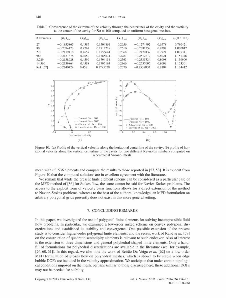
Figure 10. (a) Profile of the vertical velocity along the horizontal centerline of the cavity; (b) profile of hor-izontal velocity along the vertical centerline of the cavity for two different Reynolds numbers computed on
a centroidal Voronoi mesh.
mesh with 65, 536 elements and compare the results to those reported in [57, 58]. It is evident fromFigure 10 that the computed solutions are in excellent agreement with the literature.
We remark that while the present finite element scheme can be considered as a particular case ofthe MFD method of [36] for Stokes flow, the same cannot be said for Navier–Stokes problems. Theaccess to the explicit form of velocity basis functions allows for a direct extension of the methodto Navier–Stokes problems, whereas to the best of the authors’ knowledge, an MFD formulation onarbitrary polygonal grids presently does not exist in this more general setting.
7. CONCLUDING REMARKS
In this paper, we investigated the use of polygonal finite elements for solving incompressible fluidflow problems. In particular, we examined a low-order mixed scheme on convex polygonal dis-cretizations and established its stability and convergence. One possible extension of the presentstudy is to consider higher-order polygonal finite elements, and the recent work of Rand et al. [59]on the construction of quadratic serendipity elements is relevant to such endeavor. Also of interestis the extension to three dimensions and general polyhedral-shaped finite elements. Only a hand-ful of formulations for polyhedral discretizations are available in the literature (see, for example,[26, 60, 61]). In this regard, we also note the work of Beirão Da Veiga et al. [62] on a low-orderMFD formulation of Stokes flow on polyhedral meshes, which is shown to be stable when edgebubble DOFs are included in the velocity approximation. We anticipate that under certain topologi-cal conditions imposed on the mesh, perhaps similar to those discussed here, these additional DOFsmay not be needed for stability.
Copyright © 2013 John Wiley & Sons, Ltd. Int. J. Numer. Meth. Fluids 2014; 74:134–151DOI: 10.1002/fld

POLYGONAL FINITE ELEMENTS FOR INCOMPRESSIBLE FLUID FLOW 149
ACKNOWLEDGEMENTS
The authors appreciate constructive comments and insightful suggestions from the anonymous reviewers.Ivan F. M. Menezes and Anderson Pereira acknowledge the financial support provided by Tecgraf/PUC-Rio(Group of Technology in Computer Graphics), Rio de Janeiro, Brazil. We are thankful to the support fromthe US National Science Foundation under grant CMMI #1321661 and from the Donald B. and ElizabethM. Willett endowment at the University of Illinois at Urbana-Champaign. Any opinion, finding, conclusionsor recommendations expressed here are those of the authors and do not necessarily reflect the views ofthe sponsors.
REFERENCES
1. Girault V, Raviart PA. Finite Element Method for Navier-Stokes Equations. Springer Verlag: Berlin, 1986.2. Brezzi F, Fortin M. Mixed and Hybrid Finite Element Method. Springer: New York, 1991.3. Donea J, Huerta A. Finite Element Methods for Flow Problems. John Wiley and Sons, Ltd.: West Sussex, England,
2003.4. Ern A, Guermond JL. Theory and Practice of Finite Elements. Springer Verlag: New York, 2004.5. Boffi D, Brezzi F, Fortin M. Finite elements for the Stokes problem. Lecture Notes in Mathematics 2008;
1939:45–100.6. Babuska I. Error bounds for finite element method. Numerical Mathematics 1971; 18:322–333.7. Brezzi F. On the existence, uniqueness and approximation of saddle-point problems arising from lagrangian
multipliers. RAIRO Analyse Numérique 1974; 8(R.2):129–151.8. Arnold DN, Brezzi F, Fortin M. A stable finite element for the Stokes equations. Calcolo 1984; 21(4):
337–344.9. Hughes TJ, Franca LP, Balestra M. A new finite element formulation for computational fluid dynamics: V.
Circumventing the Babuska-Brezzi condition: a stable Petrov-Galerkin formulation of the Stokes problem accom-modating equal-order interpolations. Computer Methods in Applied Mechanics and Engineering 1986; 59(1):85–99.
10. Brezzi F, Douglas JJ. Stabilized mixed methods for the Stokes problem. Numerical Mathematics 1988; 53:225–236.
11. Barth T, Bochev P, Gunzburger M, Shadid J. A taxonomy of consistently stabilized finite element methods for theStokes problem. SIAM Journal on Scientific Computing 2004; 25(5):1585–1607.
12. Silvester D. Optimal low order finite element methods for incompressible flow. Computer Methods in AppliedMechanics and Engineering 1994; 111:357–368.
13. Bochev PB, Dohrmann CR, Gunzburger MD. Stabilization of low-order mixed finite elements for the Stokesequations. SIAM Journal on Numerical Analysis 2006; 44(1):82–101.
14. Tallec PL, Ruas V. On the convergence of the bilinear-velocity constant-pressure finite element method in viscousflow. Computer Methods in Applied Mechanics and Engineering 1986; 54(2):235–243.
15. Hauret P, Kuhl E, Ortiz M. Diamond elements: a finite element/discrete-mechanics approximation scheme withguaranteed optimal convergence in incompressible elasticity. International Journal for Numerical Methods inEngineering 2007; 72:253–294.
16. Talischi C, Paulino GH, Le CH. Honeycomb Wachspress finite elements for structural topology optimization.Structural and Multidisciplinary Optimization 2009; 37(6):569–583.
17. Talischi C, Paulino GH, Pereira A, Menezes IFM. Polygonal finite elements for topology optimization: a unifyingparadigm. International Journal for Numerical Methods in Engineering 2010; 82(6):671–698.
18. Saxena A. A material-mask overlay strategy for continuum topology optimization of compliant mechanisms usinghoneycomb discretization. Journal of Mechanical Design 2008; 130(8):082304.
19. Langelaar M. The use of convex uniform honeycomb tessellations in structural topology optimization. Proceedingsof 7th World Congress on Structural and Multidisciplinary Optimization, 2007; 21–25.
20. Jog CS, Haber RB. Stability of finite element models for distributed-parameter optimization and topology design.Computer Methods in Applied Mechanics and Engineering 1996; 130(3-4):203–226.
21. Wachspress EL. A Rational Finite Element Basis. Academic Press: New York, 1975.22. Sukumar N, Tabarraei A. Conforming polygonal finite elements. International Journal for Numerical Methods in
Engineering 2004; 61(12):2045–2066.23. Sukumar N, Malsch EA. Recent advances in the construction of polygonal finite element interpolants. Archives of
Computational Methods in Engineering 2006; 13(1):129–163.24. Ghosh S. Micromechanical Analysis and Multi-scale Modeling Using the Voronoi Cell Finite Element Method. CRC
Press: Florida, 2011.25. Talischi C, Paulino GH, Pereira A, Menezes IFM. PolyTop: A Matlab implementation of a general topology optimiza-
tion framework using unstructured polygonal finite element meshes. Structural and Multidisciplinary Optimization2012; 45:329–357.
26. Rashid MM, Selimotic M. A three-dimensional finite element method with arbitrary polyhedral elements. Interna-tional Journal for Numerical Methods in Engineering 2006; 67(2):226–252.
Copyright © 2013 John Wiley & Sons, Ltd. Int. J. Numer. Meth. Fluids 2014; 74:134–151DOI: 10.1002/fld

150 C. TALISCHI ET AL.
27. Bolander JE, Saito S. Fracture analyses using spring networks with random geometry. Engineering FractureMechanics 1998; 61(5-6):569–591.
28. Talischi C, Paulino GH, Pereira A, Menezes IFM. PolyMesher: a general-purpose mesh generator for polygonalelements written in Matlab. Structural and Multidisciplinary Optimization 2012; 45:309–328.
29. Sieger D, Alliez P, Botsch M. Optimizing Voronoi diagrams for polygonal finite element computations. Proceedingsof the 19th International Meshing Roundtable, 2010; 435–350.
30. Ebeida MS, Mitchell SA. Uniform random Voronoi meshes. Proceedings of the 20th International MeshingRoundtable, 2012; 273–290.
31. Brezzi F, Lipnikov K, Shashkov M, Simoncini V. A new discretization methodology for diffusion problems ongeneralized polyhedral meshes. Computer Methods in Applied Mechanics and Engineering 2007; 196(37-40):3682–3692.
32. Brezzi F, Buffa A, Lipnikov K. Mimetic finite differences for elliptic problems. ESAIM Mathematical Modelling andNumerical Analysis 2009; 43(02):277–295.
33. Beirão Da Veiga L, Lipnikov K, Manzini G. Arbitrary-order nodal mimetic discretizations of elliptic problems onpolygonal meshes. SIAM Journal on Numerical Analysis 2011; 49(5):1737–1760.
34. Beirão Da Veiga L, Brezzi F, Cangiani A, Manzini G, Marini LD, Russo A. Basic principles of Virtual ElementMethods. Mathematical Models and Methods in Applied Sciences 2013; 23:199–214.
35. Beirão Da Veiga L, Gyrya V, Lipnikov K, Manzini G. Mimetic finite difference method for the Stokes problem onpolygonal meshes. Journal of Computational Physics 2009; 228(19):7215–7232.
36. Beirão Da Veiga L, Lipnikov K. A mimetic discretization of the Stokes problem with selected edge bubbles. SIAMJournal on Scientific Computing 2010; 32(2):875–893.
37. Pierre R. Simple C 0 approximations for the computation of incompressible flows. Computer Methods in AppliedMechanics and Engineering 1988; 68(2):205–227.
38. Brenner SC, Scott LR. The Mathematical Theory of Finite Element Methods, 2nd ed. Springer: New York, 2002.39. Malkus DS, Olsen ET. Obtaining error estimates for optimally constrained incompressible finite elements. Computer
Methods in Applied Mechanics and Engineering 1984; 45:331–353.40. Boland J, Nicolaides R. On the stability of bilinear-constant velocity-pressure finite elements. Numerical Mathemat-
ics 1984; 44(2):219–222.41. Boland J, Nicolaides R. Stable and semistable low order finite elements for viscous flows. SIAM Journal on
Numerical Analysis 1985:474–492.42. Hughes TJR. The Finite Element Method: Linear Static and Dynamic Finite Element Analysis. Dover Publications:
New York, 2000.43. Sani RL, Gresho PM, Lee RL, Griffiths DF. The cause and cure (?) of the spurious pressures generated by certain
FEM solutions of the incompressible Navier-Stokes equations: Part 1. International Journal for Numerical Methodsin Fluids 1981; 1(1):17–43.
44. Sani RL, Gresho PM, Lee RL, Griffiths DF, Engelman M. The cause and cure (!) of the spurious pressures generatedby certain FEM solutions of the incompressible Navier-Stokes equations: Part 2. International Journal for NumericalMethods in Fluids 1981; 1(2):171–204.
45. Bochev P, Lehoucq RB. On finite element solution of the pure Neumann problem. SIAM Review 2001; 47:50–66.46. Floater MS, Hormann K, Kos G. A general construction of barycentric coordinates over convex polygons. Advances
in Computational Mathematics 2006; 24(1-4):311–331.47. Meyer M, Barr A, Lee H, Desbrun M. Generalized barycentric coordinates on irregular polygons. Journal of
Graphics Tools 2002; 7:13–22.48. Floater MS, Kosinka J. On the injectivity of Wachspress and mean value mappings between convex polygons.
Advances in Computational Mathematics 2010; 32(2):163–174.49. Gillette A, Rand A, Bajaj C. Error estimates for generalized barycentric interpolation. Advances in Computational
Mathematics 2012; 37(3):417–439.50. Mousavi SE, Xiao H, Sukumar N. Generalized Gaussian quadrature rules on arbitrary polygons. International
Journal for Numerical Methods in Engineering 2010; 82(1):99–113.51. Natarajan S, Bordas S, Mahapatra DR. Numerical integration over arbitrary polygonal domains based on Schwarz-
Christoffel conformal mapping. International Journal for Numerical Methods in Engineering 2009; 80(1):103–134.52. Yip M, Mohle J, Bolander JE. Automated modeling of three-dimensional structural components using irregular
lattices. Computer-Aided Civil and Infrastructure 2005; 20(6):393–407.53. Chapelle D, Bathe KJ. The inf-sup test. Computers and Structures 1993; 47(4-5):537–545.54. Malkus DS. Eigenproblems associated with the discrete LBB condition for incompressible finite elements.
International Journal of Engineering Science 1981; 19(10):1299–1310.55. Gerdes K, Schotzau D. hp-finite element simulations for Stokes flow – stable and stabilized. Finite Elements in
Analysis and Design 1999; 33:143–165.56. Cai Z, Wang Y. An error estimate for two-dimensional Stokes driven cavity flow. Mathematical and Computer 2009;
78(266):771–787.57. Botella O, Peyret R. Benchmark spectral results on the lid-driven cavity flow. Computers and Fluids 1998;
27(4):421–433.58. Ghia U, Ghia KN, Shin T. High-Re solutions for incompressible flow using the Navier-Stokes equations and a
multigrid method. Journal of Computational Physics 1982; 48(387-411).
Copyright © 2013 John Wiley & Sons, Ltd. Int. J. Numer. Meth. Fluids 2014; 74:134–151DOI: 10.1002/fld

POLYGONAL FINITE ELEMENTS FOR INCOMPRESSIBLE FLUID FLOW 151
59. Rand A, Gillette A, Bajaj C. Quadratic serendipity finite element on polygons using generalized barycentriccoordinates, 2012. arXiv:1109.3259v2 [math.NA].
60. Hormann K, Sukumar N. Maximum entropy coordinates for arbitrary polytopes. Eurographics Symposium onGeometry Processing 2008; 27(5).
61. Milbradt P, Pick T. Polytope finite elements. International Journal for Numerical Methods in Engineering 2008;73(12):1811–1835.
62. Beirão Da Veiga L, Lipnikov K, Manzini G. Error analysis for a mimetic discretization of the steady stokes problemon polyhedral meshes. SIAM Journal on Numerical Analysis 2010; 48(4):1419–1443.
Copyright © 2013 John Wiley & Sons, Ltd. Int. J. Numer. Meth. Fluids 2014; 74:134–151DOI: 10.1002/fld