What caused the Sacramento River fall Chinook stockcollapse?

S. T. Lindley, C. B. Grimes, M. S. Mohr, W. Peterson, J. Stein, J. T. Anderson,L. W. Botsford, , D. L. Bottom, C. A. Busack, T. K. Collier, J. Ferguson, J. C. Garza,A. M. Grover, D. G. Hankin, R. G. Kope, P. W. Lawson, A. Low, R. B. MacFar-lane, K. Moore, M. Palmer-Zwahlen, F. B. Schwing, J. Smith, C. Tracy, R. Webb,B. K. Wells, T. H. Williams

Pre-publication report to the Pacific Fishery Management Council

March 18, 2009

1

Contents1 Executive summary 4

2 Introduction 7

3 Analysis of recent broods 103.1 Review of the life history of SRFC . . . . . . . . . . . . . . . . . . 103.2 Available data . . . . . . . . . . . . . . . . . . . . . . . . . . . . . 113.3 Conceptual approach . . . . . . . . . . . . . . . . . . . . . . . . . 113.4 Brood year 2004 . . . . . . . . . . . . . . . . . . . . . . . . . . . 15

3.4.1 Parents . . . . . . . . . . . . . . . . . . . . . . . . . . . . 153.4.2 Eggs . . . . . . . . . . . . . . . . . . . . . . . . . . . . . 163.4.3 Fry, parr and smolts . . . . . . . . . . . . . . . . . . . . . . 173.4.4 Early ocean . . . . . . . . . . . . . . . . . . . . . . . . . . 213.4.5 Later ocean . . . . . . . . . . . . . . . . . . . . . . . . . . 303.4.6 Spawners . . . . . . . . . . . . . . . . . . . . . . . . . . . 323.4.7 Conclusions for the 2004 brood . . . . . . . . . . . . . . . 32

3.5 Brood year 2005 . . . . . . . . . . . . . . . . . . . . . . . . . . . 333.5.1 Parents . . . . . . . . . . . . . . . . . . . . . . . . . . . . 333.5.2 Eggs . . . . . . . . . . . . . . . . . . . . . . . . . . . . . 333.5.3 Fry, parr and smolts . . . . . . . . . . . . . . . . . . . . . . 333.5.4 Early ocean . . . . . . . . . . . . . . . . . . . . . . . . . . 343.5.5 Later ocean . . . . . . . . . . . . . . . . . . . . . . . . . . 353.5.6 Spawners . . . . . . . . . . . . . . . . . . . . . . . . . . . 353.5.7 Conclusions for the 2005 brood . . . . . . . . . . . . . . . 35

3.6 Prospects for brood year 2006 . . . . . . . . . . . . . . . . . . . . 363.7 Is climate change a factor? . . . . . . . . . . . . . . . . . . . . . . 363.8 Summary . . . . . . . . . . . . . . . . . . . . . . . . . . . . . . . 37

4 The role of anthropogenic impacts 384.1 Sacramento River fall Chinook . . . . . . . . . . . . . . . . . . . . 384.2 Other Chinook stocks in the Central Valley . . . . . . . . . . . . . 43

5 Recommendations 475.1 Knowledge Gaps . . . . . . . . . . . . . . . . . . . . . . . . . . . 475.2 Improving resilience . . . . . . . . . . . . . . . . . . . . . . . . . 485.3 Synthesis . . . . . . . . . . . . . . . . . . . . . . . . . . . . . . . 49

2

List of Figures1 Sacramento River index. . . . . . . . . . . . . . . . . . . . . . . . 82 Map of the Sacramento River basin and adjacent coastal ocean. . . . 133 Conceptual model of a cohort of fall-run Chinook. . . . . . . . . . . 144 Discharge in regulated reaches of the Sacramento River, Feather

River, American River and Stanislaus River in 2004-2007. . . . . . 165 Daily export of freshwater from the Delta and the ratio of exports

to inflows. . . . . . . . . . . . . . . . . . . . . . . . . . . . . . . . 186 Releases of hatchery fish. . . . . . . . . . . . . . . . . . . . . . . . 197 Mean annual catch-per-unit effort of fall Chinook juveniles at Chipps

Island by USFWS trawl sampling. . . . . . . . . . . . . . . . . . . 208 Cumulative daily catch per unit effort of fall Chinook juveniles at

Chipps Island by USFWS trawl sampling in 2005. . . . . . . . . . . 209 Relative survival from release into the estuary to age two in the

ocean for Feather River Hatchery fall Chinook. . . . . . . . . . . . 2210 Escapement of SRFC jacks. . . . . . . . . . . . . . . . . . . . . . . 2211 Conceptual diagram displaying the hypothesized relationship be-

tween wind-forced upwelling and the pelagic ecosystem. . . . . . . 2412 Sea surface temperature (colors) and wind (vectors) anomalies for

the north Pacific for Apr-Jun in 2005-2008. . . . . . . . . . . . . . 2513 Cumulative upwelling index (CUI) and anomalies of the CUI. . . . 2714 Sea surface temperature anomalies off central California in May-

July of 2003-2006. . . . . . . . . . . . . . . . . . . . . . . . . . . 2815 Surface particle trajectories predicted from the OSCURS current

model . . . . . . . . . . . . . . . . . . . . . . . . . . . . . . . . . 2916 Length, weight and condition factor of juvenile Chinook over the

1998-2005 period. . . . . . . . . . . . . . . . . . . . . . . . . . . . 3117 Changes in interannual variation in summer and winter upwelling

at 39◦N latitude. . . . . . . . . . . . . . . . . . . . . . . . . . . . . 3719 The fraction of total escapement of SRFC that returns to spawn in

hatcheries. . . . . . . . . . . . . . . . . . . . . . . . . . . . . . . . 4220 Escapement trends in various populations of Central Valley Chinook. 4521 Escapement trends in the 1990s and 2000s of various populations

of Chinook. . . . . . . . . . . . . . . . . . . . . . . . . . . . . . . 46

List of Tables1 Summary of data sources used in this report. . . . . . . . . . . . . . 12

3

1 Executive summary1

In April 2008, in response to the sudden collapse of Sacramento River fall Chi-2

nook salmon (SRFC) and the poor status of many west coast coho salmon popula-3

tions, the Pacific Fishery Management Council (PFMC) adopted the most restric-4

tive salmon fisheries in the history of the west coast of the U.S. The regulations5

included a complete closure of commercial and recreational Chinook salmon fish-6

eries south of Cape Falcon, Oregon. Spawning escapement of SRFC in 2007 is es-7

timated to have been 88,000, well below the PFMC’s escapement conservation goal8

of 122,000-180,000 for the first time since the early 1990s. The situation was even9

more dire in 2008, when 66,000 spawners are estimated to have returned to natural10

areas and hatcheries. For the SRFC stock, which is an aggregate of hatchery and11

natural production, many factors have been suggested as potential causes of the poor12

escapements, including freshwater withdrawals (including pumping of water from13

the Sacramento-San Joaquin delta), unusual hatchery events, pollution, elimination14

of net-pen acclimatization facilities coincident with one of the two failed brood15

years, and large-scale bridge construction during the smolt outmigration (CDFG,16

2008). In this report we review possible causes for the decline in SRFC for which17

reliable data were available.18

Our investigation was guided by a conceptual model of the life history of fall19

Chinook salmon in the wild and in the hatchery. Our approach was to identify where20

and when in the life cycle abundance became anomalously low, and where and when21

poor environmental conditions occurred due to natural or human-induced causes.22

The likely cause of the SRFC collapse lies at the intersection of an unusually large23

drop in abundance and poor environmental conditions. Using this framework, all of24

the evidence that we could find points to ocean conditions as being the proximate25

cause of the poor performance of the 2004 and 2005 broods of SRFC. We recognize,26

however, that the rapid and likely temporary deterioration in ocean conditions is27

acting on top of a long-term, steady degradation of the freshwater and estuarine28

environment.29

The evidence pointed to ocean conditions as the proximate cause because con-30

ditions in freshwater were not unusual, and a measure of abundance at the entrance31

to the estuary showed that, up until that point, these broods were at or near normal32

levels of abundance. At some time and place between this point and recruitment to33

the fishery at age two, unusually large fractions of these broods perished. A broad34

body of evidence suggests that anomalous conditions in the coastal ocean in 200535

and 2006 resulted in unusually poor survival of the 2004 and 2005 broods of SRFC.36

Both broods entered the ocean during periods of weak upwelling, warm sea surface37

temperatures, and low densities of prey items. Individuals from the 2004 brood38

sampled in the Gulf of the Farallones were in poor physical condition, indicating39

that feeding conditions were poor in the spring of 2005 (unfortunately, comparable40

data do not exist for the 2005 brood). Pelagic seabirds in this region with diets sim-41

ilar to juvenile Chinook salmon also experienced very poor reproduction in these42

years. In addition, the cessation of net-pen acclimatization in the estuary in 200643

may have contributed to the especially poor estuarine and marine survival of the44

4

2005 brood.45

Fishery management also played a role in the low escapement of 2007. The46

PFMC (2007) forecast an escapement of 265,000 SRFC adults in 2007 based on47

the escapement of 14,500 Central Valley Chinook salmon jacks in 2006. The real-48

ized escapement of SRFC adults was 87,900. The large discrepancy between the49

forecast and realized abundance was due to a bias in the forecast model that has50

since been corrected. Had the pre-season ocean abundance forecast been more ac-51

curate and fishing opportunity further constrained by management regulation, the52

SRFC escapement goal could have been met in 2007. Thus, fishery management,53

while not the cause of the 2004 brood weak year-class strength, contributed to the54

failure to achieve the SRFC escapement goal in 2007.55

The long-standing and ongoing degradation of freshwater and estuarine habitats56

and the subsequent heavy reliance on hatchery production were also likely contrib-57

utors to the collapse of the stock. Degradation and simplification of freshwater58

and estuary habitats over a century and a half of development have changed the59

Central Valley Chinook salmon complex from a highly diverse collection of nu-60

merous wild populations to one dominated by fall Chinook salmon from four large61

hatcheries. Naturally-spawning populations of fall Chinook salmon are now ge-62

netically homogeneous in the Central Valley, and their population dynamics have63

been synchronous over the past few decades. In contrast, some remnant populations64

of late-fall, winter and spring Chinook salmon have not been as strongly affected65

by recent changes in ocean conditions, illustrating that life-history diversity can66

buffer environmental variation. The situation is analogous to managing a financial67

portfolio: a well-diversified portfolio will be buffeted less by fluctuating market68

conditions than one concentrated on just a few stocks; the SRFC seems to be quite69

concentrated indeed.70

Climate variability plays an important role in the inter-annual variation in abun-71

dance of Pacific salmon, including SRFC. We have observed a trend of increasing72

variability over the past several decades in climate indices related to salmon sur-73

vival. This is a coast-wide pattern, but may be particularly important in California,74

where salmon are near the southern end of their range. These more extreme climate75

fluctuations put additional strain on salmon populations that are at low abundance76

and have little life-history or habitat diversity. If the trend of increasing climate77

variability continues, then we can expect to see more extreme variation in the abun-78

dance of SRFC and salmon stocks coast wide.79

In conclusion, the development of the Sacramento-San Joaquin watershed has80

greatly simplified and truncated the once-diverse habitats that historically supported81

a highly diverse assemblage of populations. The life history diversity of this histor-82

ical assemblage would have buffered the overall abundance of Chinook salmon in83

the Central Valley under varying climate conditions. We are now left with a fish-84

ery that is supported largely by four hatcheries that produce mostly fall Chinook85

salmon. Because the survival of fall Chinook salmon hatchery release groups is86

highly correlated among nearby hatcheries, and highly variable among years, we87

can expect to see more booms and busts in this fishery in the future in response88

to variation in the ocean environment. Simply increasing the production of fall89

5

Chinook salmon from hatcheries as they are currently operated may aggravate this90

situation by further concentrating production in time and space. Rather, the key to91

reducing variation in production is increasing the diversity of SRFC.92

There are few direct actions available to the PFMC to improve this situation,93

but there are actions the PFMC can support that would lead to increased diversity94

of SRFC and increased stability. Mid-term solutions include continued advocacy95

for more fish-friendly water management and the examination of hatchery prac-96

tices to improve the survival of hatchery releases while reducing adverse interac-97

tions with natural fish. In the longer-term, increased habitat quantity, quality, and98

diversity, and modified hatchery practices could allow life history diversity to in-99

crease in SRFC. Increased diversity in SRFC life histories should lead to increased100

stability and resilience in a dynamic, changing environment. Using an ecosystem-101

based management and ecological risk assessment framework to engage the many102

agencies and stakeholder groups with interests in the ecosystems supporting SRFC103

would aid implementation of these solutions.104

6

2 Introduction105

In April 2008 the Pacific Fishery Management Council (PFMC) adopted the most106

restrictive salmon fisheries in the history of the west coast of the U.S., in response to107

the sudden collapse of Sacramento River fall Chinook (SRFC) salmon and the poor108

status of many west coast coho salmon populations. The PFMC adopted a com-109

plete closure of commercial and recreational Chinook fisheries south of Cape Fal-110

con, Oregon, allowing only for a mark-selective hatchery coho recreational fishery111

of 9,000 fish from Cape Falcon, Oregon, to the Oregon/California border. Salmon112

fisheries off California and Oregon have historically been robust, with seasons span-113

ning May through October and catches averaging over 800,000 Chinook per year114

from 2000 to 2005. The negative economic impact of the closure was so drastic115

that west coast Governors asked for $290 million in disaster relief, and the U.S.116

Congress appropriated $170 million.117

Escapement of several west coast Chinook and coho salmon stocks was lower118

than expected in 2007 (PFMC, 2009), and low jack escapement in 2007 for some119

stocks suggested that 2008 would be at least as bad (PFMC, 2008). The most120

prominent example is SRFC salmon, for which spawning escapement in 2007 is121

estimated to have been 88,000, well below the escapement conservation goal of122

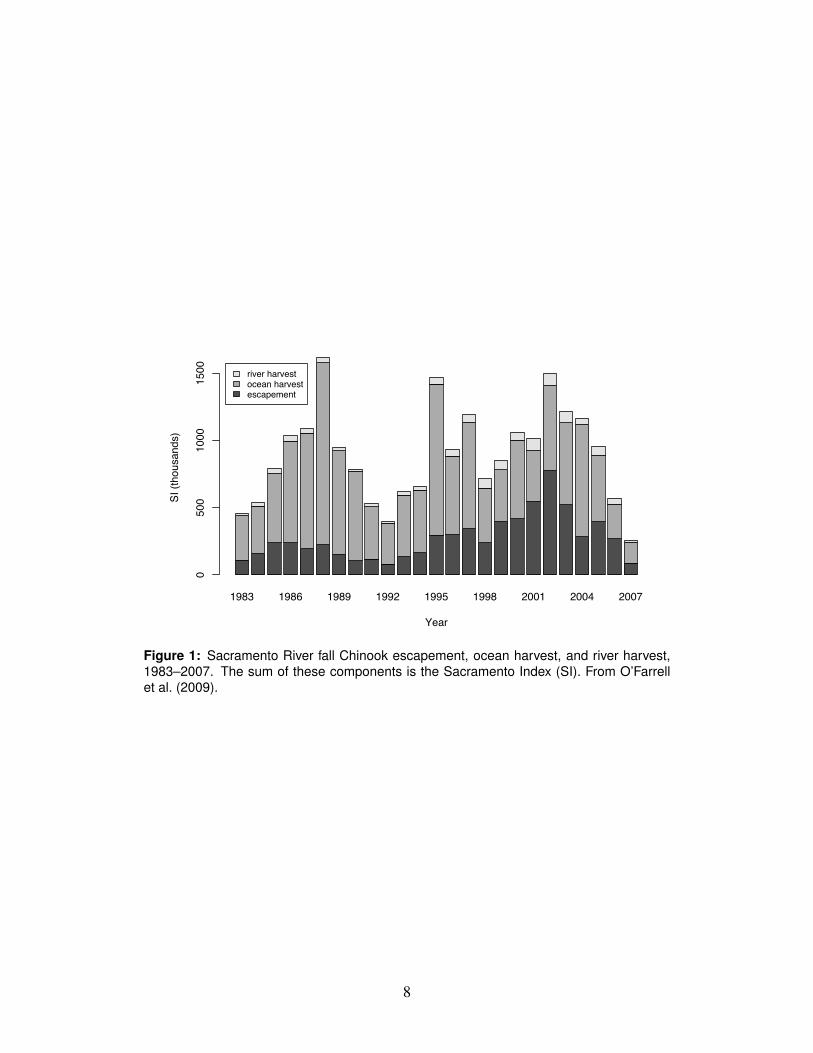
the PFMC (122,000–180,000 fish) for the first time since the early 1990s (Fig. 1).123

While the 2007 escapement represents a continuing decline since the recent peak124

escapement of 725,000 spawners in 2002, average escapement since 1983 has been125

about 248,000. The previous record low escapement, observed in 1992, is believed126

to have been due to a combination of drought conditions, overfishing, and poor127

ocean conditions (SRFCRT, 1994). Although conditions have been wetter than av-128

erage over the 2000-2005 period, the spawning escapement of jacks in 2007 was129

the lowest on record, significantly lower than the 2006 jack escapement (the second130

lowest on record), and the preseason projection of 2008 adult spawner escapement131

was only 59,0001 despite the complete closure of coastal and freshwater Chinook132

fisheries.133

Low escapement has also been documented for coastal coho salmon during this134

same time frame. For California, coho salmon escapement in 2007 averaged 27%135

of parent stock abundance in 2004, with a range from 0% (Redwood Creek) to 68%136

(Shasta River). In Oregon, spawner estimates for the Oregon Coast natural (OCN)137

coho salmon were 30% of parental spawner abundance. These returns are the lowest138

since 1999, and are near the low abundances of the 1990s. Columbia River coho139

and Chinook stocks experienced mixed escapement in 2007 and 2008.140

For coho salmon in 2007 there was a clear north-south gradient, with escape-141

ment improving to the north. California and Oregon coastal escapement was down142

sharply, while Columbia River hatchery coho were down only slightly (PFMC,143

2009). Washington coastal coho escapement was similar to 2006. Even within144

the OCN region, there was a clear north-south pattern, with the north coast region145

(predominantly Nehalem River and Tillamook Bay populations) returning at 46%146

1Preliminary postseason estimate for 2008 SRFC adult escapement is 66,000.

7

1983 1986 1989 1992 1995 1998 2001 2004 2007

Year

SI (t

hous

ands

)

050

010

0015

00 river harvestocean harvestescapement

Figure 1: Sacramento River fall Chinook escapement, ocean harvest, and river harvest,1983–2007. The sum of these components is the Sacramento Index (SI). From O’Farrellet al. (2009).

8

of parental abundance while the mid-south coast region (predominantly Coos and147

Coquille populations) returned at only 14% of parental abundance. The Rogue148

River population was only 21% of parental abundance. Low 2007 jack escapement149

for these three stocks in particular suggests a continued low abundance in 2008.150

In addition, Columbia River coho salmon jack escapement in 2007 was also near151

record lows.152

There have been exceptions to these patterns of decline. Klamath River fall153

Chinook experienced a very strong 2004 brood, despite parent spawners being well154

below the estimated level necessary for maximum production. Columbia River155

spring Chinook production from the 2004 and 2005 broods will be at historically156

high levels, according to age-class escapement to date. The 2008 forecasts for157

Columbia River fall Chinook “tule” stocks are significantly more optimistic than158

for 2007. Curiously, Sacramento River late-fall Chinook escapement has declined159

only modestly since 2002, while the SRFC in the same river basin fell to record low160

levels.161

What caused the observed general pattern of low salmon escapement? For the162

SRFC stock, which is an aggregate of hatchery and natural production (but prob-163

ably dominated by hatchery production (Barnett-Johnson et al., 2007)), freshwater164

withdrawals (including pumping of water from the Sacramento-San Joaquin Delta),165

unusual hatchery events, pollution, elimination of net-pen acclimatization facilities166

coincident with one of the two failed brood years, and large-scale bridge construc-167

tion during the smolt outmigration along with many other possibilities have been168

suggested as prime candidates causing the poor escapement (CDFG, 2008).169

When investigating the possible causes for the decline of SRFC, we need to rec-170

ognize that salmon exhibit complex life histories, with potential influences on their171

survival at a variety of life stages in freshwater, estuarine and marine habitats. Thus,172

salmon typically have high variation in adult escapement, which may be explained173

by a variety of anthropogenic and natural environmental factors. Also, environ-174

mental change affects salmon in different ways at different time scales. In the short175

term, the dynamics of salmon populations reflect the effects of environmental vari-176

ation, e.g., high freshwater flows during the outmigration period might increase177

juvenile survival and enhance recruitment to the fishery. On longer time scales,178

the cumulative effects of habitat degradation constrain the diversity and capacity of179

habitats, extirpating some populations and reducing the diversity and productivity180

of surviving populations (Bottom et al., 2005b). This problem is especially acute in181

the Sacramento-San Joaquin basin, where the effects of land and water development182

have extirpated many populations of spring-, winter- and late-fall-run Chinook and183

reduced the diversity and productivity of fall Chinook populations (Myers et al.,184

1998; Good et al., 2005; Lindley et al., 2007).185

Focusing on the recent variation in salmon escapement, the coherence of varia-186

tions in salmon productivity over broad geographic areas suggests that the patterns187

are caused by regional environmental variation. This could include such events188

as widespread drought or floods affecting hydrologic conditions (e.g., river flow189

and temperature), or regional variation in ocean conditions (e.g., temperature, up-190

welling, prey and predator abundance). Variations in ocean climate have been in-191

9

creasingly recognized as an important cause of variability in the landings, abun-192

dance, and productivity of salmon (e.g, Hare and Francis (1995); Mantua et al.193

(1997); Beamish et al. (1999); Hobday and Boehlert (2001); Botsford and Lawrence194

(2002); Mueter et al. (2002); Pyper et al. (2002)). The Pacific Ocean has many195

modes of variation in sea surface temperature, mixed layer depth, and the strength196

and position of winds and currents, including the El Nino-Southern Oscillation, the197

Pacific Decadal Oscillation and the Northern Oscillation. The broad variation in198

physical conditions creates corresponding variation in the pelagic food webs upon199

which juvenile salmon depend, which in turn creates similar variation in the popula-200

tion dynamics of salmon across the north Pacific. Because ocean climate is strongly201

coupled to the atmosphere, ocean climate variation is also related to terrestrial cli-202

mate variation (especially precipitation). It can therefore be quite difficult to tease203

apart the roles of terrestrial and ocean climate in driving variation in the survival204

and productivity of salmon (Lawson et al., 2004).205

In this report we review possible causes for the decline in SRFC, limiting our206

analysis to those potential causes for which there are reliable data to evaluate. First,207

we analyze the performance of the 2004, 2005 and 2006 broods of SRFC and look208

for corresponding conditions and events in their freshwater, estuarine and marine209

environments. Then we discuss the impact of long-term degradation in freshwater210

and estuarine habitats and the effects of hatchery practices on the biodiversity of211

Chinook in the Central Valley, and how reduced biodiversity may be making Chi-212

nook fisheries more susceptible to variations in ocean and terrestrial climate. We213

end the report with recommendations for future monitoring, research, and conser-214

vation actions. The appendix answers each of the more than 40 questions posed to215

the committee and provides summaries of most of the data used in the main report216

(CDFG, 2008).217

3 Analysis of recent broods218

3.1 Review of the life history of SRFC219

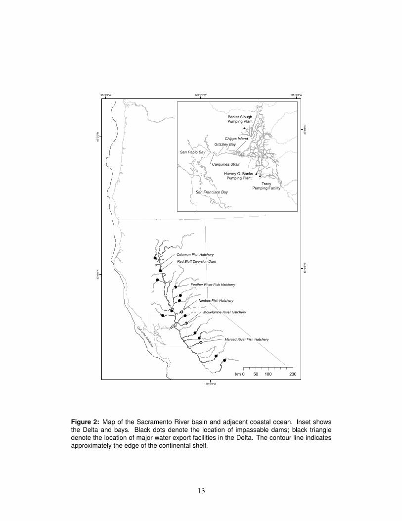
Naturally spawning SRFC return to the spawning grounds in the fall and lay their220

eggs in the low elevation areas of the Sacramento River and its tributaries (Fig. 2).221

Eggs incubate for a month or more in the fall or winter, and fry emerge and rear222

throughout the rivers, tributaries and the Delta in the late winter and spring. In May223

or June, the juveniles are ready for life in the ocean, and migrate into the estuary224

(Suisun Bay to San Francisco Bay) and on to the Gulf of the Farallones. Emigra-225

tion from freshwater is complete by the end of June, and juveniles migrate rapidly226

through the estuary (MacFarlane and Norton, 2002). While information specific to227

the distribution of SRFC during early ocean residence is mostly lacking, fall Chi-228

nook in Oregon and Washington reside very near shore (even within the surf zone)229

and near their natal river for some time after ocean entry, before moving away230

from the natal river mouth and further from shore (Brodeur et al., 2004). SRFC231

are encountered in ocean salmon fisheries in coastal waters mainly between cen-232

10

tral California and northern Oregon (O’Farrell et al., 2009; Weitkamp, In review),233

with highest abundances around San Francisco. Most SRFC return to freshwater to234

spawn after two or three years of feeding in the ocean.235

A large portion of the SRFC contributing to ocean fisheries is raised in hatcheries236

(Barnett-Johnson et al., 2007), including Coleman National Fish Hatchery (CNFH)237

on Battle Creek, Feather River Hatchery (FRH), Nimbus Hatchery on the Amer-238

ican River, and the Mokelumne River Hatchery. Hatcheries collect fish that as-239

cend hatchery weirs, breed them, and raise progeny to the smolt stage. The state240

hatcheries transport >90% of their production to the estuary in trucks, where some241

smolts usually are acclimatized briefly in net pens and others released directly into242

the estuary; Coleman National Fish Hatchery (CNFH) usually releases its produc-243

tion directly into Battle Creek.244

3.2 Available data245

A large number of datasets are potentially relevant to the investigation at hand.246

These are summarized in Table 1.247

3.3 Conceptual approach248

The poor landings and escapement of Chinook in 2007 and the record low escape-249

ment in 2008 suggests that something unusual happened to the SRFC 2004 and250

2005 broods, and more than forty possible causes for the decline were evaluated251

by the committee. Poor survival of a cohort can result from poor survival at one or252

more stages in the life cycle. Life cycle stages occur at certain times and places, and253

an examination of possible causes of poor survival should account for the temporal254

and spatial distribution of these life stages. It is helpful to consider a conceptual255

model of a cohort of fall-run Chinook that illustrates how various anthropogenic256

and natural factors affect the cohort (Fig. 3). The field of candidate causes can be257

narrowed by looking at where in the life cycle the abundance of the cohort became258

unusually low, and by looking at which of the causal factors were at unusual levels259

for these broods. The most likely causes of the decline will be those at unusual260

levels at a time and place consistent with the unusual change in abundance.261

In this report, we trace through the life cycle of each cohort, starting with the262

parents of the cohort and ending with the return of the adults. Coverage of life stages263

and possible causes for the decline varies in depth, partly due to differences in the264

information available and partly to the committee’s belief in the likelihood that265

particular life stages and causal mechanisms are implicated in the collapse. Each266

potential factors identified by CDFG (2008) is, however, addressed individually in267

the Appendix. Before we delve into the details of each cohort, it is worthwhile to268

list some especially pertinent observations relative to the 2004 and 2005 broods:269

• Near-average numbers of fall Chinook juveniles were captured at Chipps Is-270

land271

11

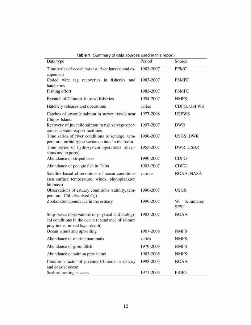
Table 1: Summary of data sources used in this report.Data type Period Source

Time series of ocean harvest, river harvest and es-capement

1983-2007 PFMC

Coded wire tag recoveries in fisheries andhatcheries

1983-2007 PSMFC

Fishing effort 1983-2007 PSMFC

Bycatch of Chinook in trawl fisheries 1994-2007 NMFS

Hatchery releases and operations varies CDFG, USFWS

Catches of juvenile salmon in survey trawls nearChipps Island

1977-2008 USFWS

Recovery of juvenile salmon in fish salvage oper-ations at water export facilities

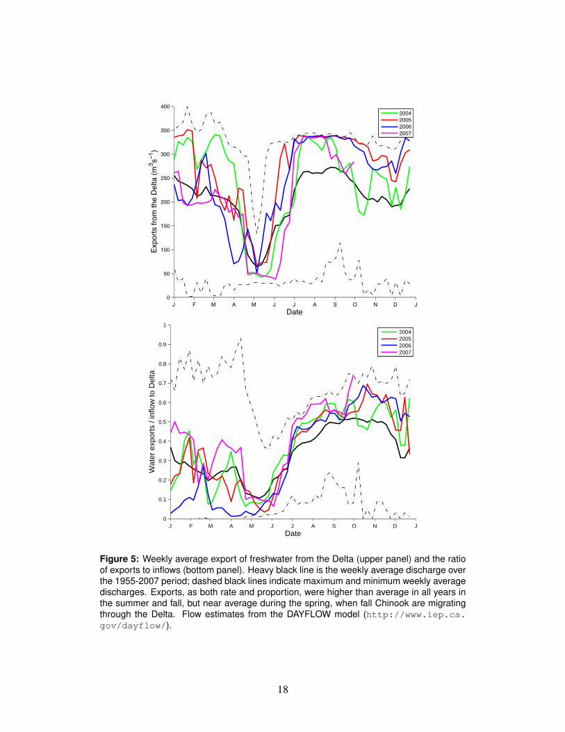
1997-2007 DWR

Time series of river conditions (discharge, tem-perature, turbidity) at various points in the basin

1990-2007 USGS, DWR

Time series of hydrosystem operations (diver-sions and exports)

1955-2007 DWR, USBR

Abundance of striped bass 1990-2007 CDFG

Abundance of pelagic fish in Delta 1993-2007 CDFG

Satellite-based observations of ocean conditions(sea surface temperature, winds, phytoplanktonbiomass)

various NOAA, NASA

Observations of estuary conditions (salinity, tem-perature, Chl, dissolved O2)

1990-2007 USGS

Zoolankton abundance in the estuary 1990-2007 W. Kimmerer,SFSU

Ship-based observations of physical and biologi-cal conditions in the ocean (abundance of salmonprey items, mixed layer depth)

1983-2007 NOAA

Ocean winds and upwelling 1967-2008 NMFS

Abundance of marine mammals varies NMFS

Abundance of groundfish 1970-2005 NMFS

Abundance of salmon prey items 1983-2005 NMFS

Condition factor of juvenile Chinook in estuaryand coastal ocean

1998-2005 NOAA

Seabird nesting success 1971-2005 PRBO

12

Nimbus Fish Hatchery

Coleman Fish Hatchery

Mokelumne River Hatchery

Merced River Fish Hatchery

Feather River Fish Hatchery

Gulf of the Farallones

Red Bluff Diversion Dam

!

!

!

!

!

!

!

!

!

!

!!

!

!!

!(

!(

!(

!(

!(

!

115°0'0"W

120°0'0"W

120°0'0"W125°0'0"W45

°0'0"N 45

°0'0"N

40°0'

0"N 40°0'

0"N

#

#

#

TracyPumping Facility

Barker SloughPumping Plant

Harvey O. Banks Pumping Plant

San Pablo Bay

Carquinez Strait

San Francisco Bay

Grizzley BayChipps Island

0 100 20050km

Figure 2: Map of the Sacramento River basin and adjacent coastal ocean. Inset showsthe Delta and bays. Black dots denote the location of impassable dams; black triangledenote the location of major water export facilities in the Delta. The contour line indicatesapproximately the edge of the continental shelf.

13

parents

eggs

fry

smolts

age 2

age 3

eggs

fry

smolts

diseasewater quality

diseasewater quality

diseasewater qualityfeed

diseasenet penstrucks

high templow flowsdisease

scourstrandinghigh tempdisease

entrainment

lethal noise

release timingsize at release

poor feedingpredation

predation

fishing

terrestrial/fw climate

bridge construction

hydro ops

hydro ops

marine climate

birds, fish, mammals

fish, birds

pollutiondisease

diseasepestisidespredation

parents

agriculture

oil spills

BY

+3B

Y+2

sprin

g, B

Y +1

win

ter,

BY

+1fa

ll, B

Y

timeline

predation

fishing

recruitment

In Captivity In Nature

Figure 3: Conceptual model of a cohort of fall-run Chinook and the factors affecting itssurvival. Orange boxes represent life stages in the hatchery, and black boxes represent lifestages in the wild.

14

• Near-average numbers of SRFC smolts were released from state and federal272

hatcheries273

• Hydrologic conditions in the river and estuary were not unusual during the274

juvenile rearing and outmigration periods (in particular, drought conditions275

were not in effect)276

• Although water exports reaches record levels in 2005 and 2006, these lev-277

els were not reached until June and July, a period of time which followed278

outmigration of the vast majority of fall Chinook salmon smolts from the279

Sacramento system280

• Survival of Feather River fall Chinook from release into the estuary to re-281

cruitment to fisheries at age two was extremely poor282

• Physical and biological conditions in the ocean appeared to be unusually poor283

for juvenile Chinook in the spring of 2005 and 2006284

• Returns of Chinook and coho salmon to many other basins in California,285

Oregon and Washington were also low in 2007 and 2008.286

From these facts, we infer that unfavorable conditions during the early marine287

life of the 2004 and 2005 broods is likely the cause of the stock collapse. Fresh-288

water factors do not appear to be implicated directly because of the near average289

abundance of smolts at Chipps Island and because tagged fish released into the es-290

tuary had low survival to age two. Marine factors are further implicated by poor291

returns of coho and Chinook in other west coast river basins and numerous obser-292

vations of anomalous conditions in the California Current ecosystem, especially293

nesting failure of seabirds that have a diet and distribution similar to that of juvenile294

salmon.295

In the remainder of this section, we follow each brood through its lifecycle,296

bringing relatively more detail to the assessment of ocean conditions during the297

early marine phase of the broods. While we are confident that ocean conditions are298

the proximate cause of the poor performance of the 2004 and 2005 broods, human299

activities in the freshwater environment have played an important role in creating a300

stock that is vulnerable to episodic crashes; we develop this argument in section 4.301

3.4 Brood year 2004302

3.4.1 Parents303

The possible influences on the 2004 brood of fall-run Chinook began in 2004, with304

the maturation, upstream migration and spawning of the brood’s parents. Most sig-305

nificantly, 203,000 adult fall Chinook returned to spawn in the Sacramento River306

and its tributaries in 2004, slightly more than the 1970-2007 mean of 195,000; es-307

capement to the Sacramento basin hatcheries totaled 80,000 adults (PFMC, 2009).308

In September and October of 2004, water temperatures were elevated by about309

15

J F M A M J J A S O N D J F0

500

1000

1500

2000

2500

3000Sacramento R. (BND)

Date

Dis

char

ge (

m3 s−

1 )

J F M A M J J A S O N D J F0

1000

2000

3000

4000Feather R (GRL)

Date

Dis

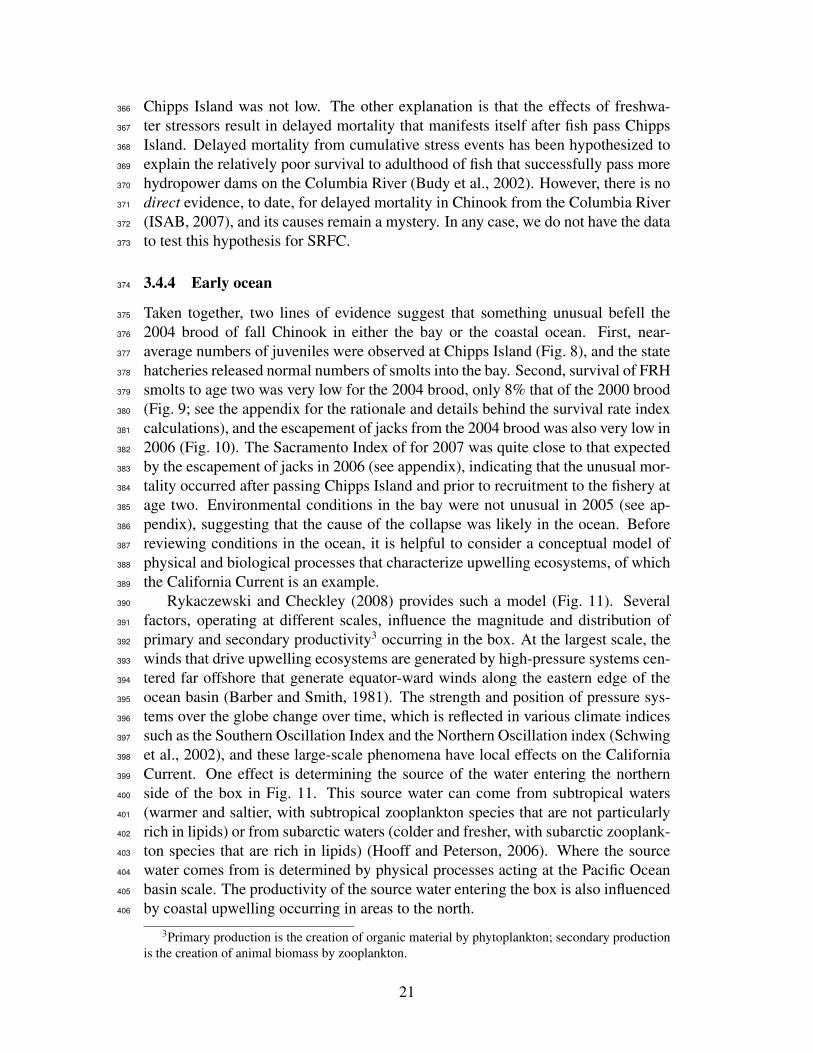
char

ge (

m3 s−

1 )

2004200520062007

J F M A M J J A S O N D J F0

50

100

150

200

250

300American R (NAT)

Date

Dis

char

ge (

m3 s−

1 )

J F M A M J J A S O N D J F0

50

100

150

200Stanislaus R (RIP)

Date

Dis

char

ge (

m3 s−

1 )

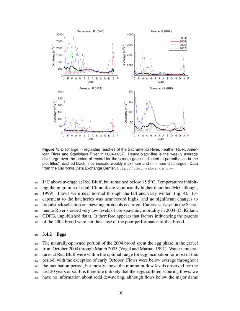
Figure 4: Discharge in regulated reaches of the Sacramento River, Feather River, Amer-ican River and Stanislaus River in 2004-2007. Heavy black line is the weekly averagedischarge over the period of record for the stream gage (indicated in parentheses in theplot titles); dashed black lines indicate weekly maximum and minimum discharges. Datafrom the California Data Exchange Center, http://cdec.water.ca.gov.

1◦C above average at Red Bluff, but remained below 15.5◦C. Temperatures inhibit-310

ing the migration of adult Chinook are significantly higher than this (McCullough,311

1999). Flows were near normal through the fall and early winter (Fig. 4). Es-312

capement to the hatcheries was near record highs, and no significant changes to313

broodstock selection or spawning protocols occurred. Carcass surveys on the Sacra-314

mento River showed very low levels of pre-spawning mortality in 2004 (D. Killam,315

CDFG, unpublished data). It therefore appears that factors influencing the parents316

of the 2004 brood were not the cause of the poor performance of that brood.317

3.4.2 Eggs318

The naturally-spawned portion of the 2004 brood spent the egg phase in the gravel319

from October 2004 through March 2005 (Vogel and Marine, 1991). Water tempera-320

tures at Red Bluff were within the optimal range for egg incubation for most of this321

period, with the exception of early October. Flows were below average throughout322

the incubation period, but mostly above the minimum flow levels observed for the323

last 20 years or so. It is therefore unlikely that the eggs suffered scouring flows; we324

have no information about redd dewatering, although flows below the major dams325

16

are regulated to prevent significant redd dewatering.326

In the hatcheries, no unusual events were noted during the incubation of the327

eggs of the 2004 brood. Chemical treatments of the eggs were not changed for the328

2004 brood.329

3.4.3 Fry, parr and smolts330

As noted above, flows in early 2005 were relatively low until May, when conditions331

turned wet and flows rose to above-normal levels (Fig. 4). Higher spring flows332

are associated with higher survival of juvenile salmon (Newman and Rice, 2002).333

Water temperature at Red Bluff was above the 1990-2007 average for much of the334

winter and spring, but below temperatures associated with lower survival of juvenile335

life stages (McCullough, 1999). In 2005, the volume of water pumped from the336

Delta reached record levels in January before falling to near-average levels in the337

spring, then rising again to near-record levels in the summer and fall (Fig. 5,top), but338

only after the migration of fall Chinook smolts was nearly complete (Fig. 8). Water339

diversions, in terms of the export:inflow ratio (E/I), fluctuated around the average340

throughout the winter and spring (Fig. 5,bottom). Statistical analysis of coded-341

wire-tagged releases of Chinook to the Delta have shown that survival declines342

with increasing exports and increasing E/I at time of release (Kjelson and Brandes,343

1989; Newman and Rice, 2002).344

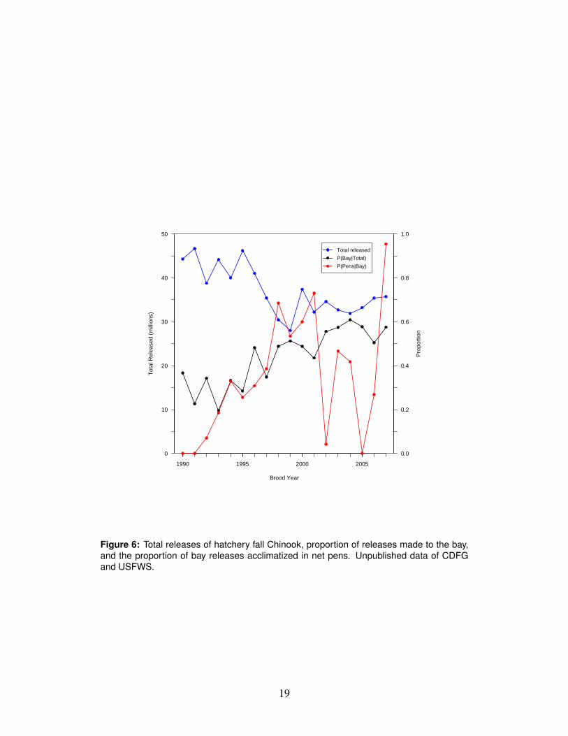
Releases of Chinook smolts were at typical levels for the 2004 brood, with a345

high proportion released into the bay, and of these, a not-unusual portion acclima-346

tized in net pens prior to release (Fig. 6). No significant disease outbreaks or other347

problems with the releases were noted.348

Systematic trawl sampling near Chipps Island provides an especially useful349

dataset for assessing the strength of a brood as it enters the estuary2. The US-350

FWS typically conducts twenty-minute mid-water trawls, 10 times per day, 5 days351

a week. An index of abundance can be formed by dividing the total catch per day by352

the total volume swept by the trawl gear. Fig. 7 shows the mean annual CPUE from353

1976 to 2007; CPUE in 2005 was slightly above average. The timing of catches354

of juvenile fall Chinook at Chipps Island was not unusual in 2005 (Fig. 8). Had355

the survival of the 2004 brood been unusually poor in freshwater, catches at Chipps356

Island should have been much lower than average, since by reaching that location,357

fish have survived almost all of the freshwater phase of their juvenile life.358

There are two reasons, however, that apparently normal catches at Chipps Island359

could mask negative impacts that occurred in freshwater. One possibility is that360

catches were normal because the capture efficiency of the trawl was much higher361

than usual. The capture efficiency of the trawl, as estimated by the recovery rate362

of coded-wire-tagged Chinook, is variable among years, but the recovery rate of363

Chinook released at Ryde in 2005 was about average (P. Brandes, USFWS, un-364

published data). This suggests that the actual abundance of fall Chinook passing365

2Catches at Chipps Island include naturally-produced fish and CNFH hatchery fish released atBattle Creek; almost all fish from the state hatcheries are released downstream of Chipps Island.

17

J F M A M J J A S O N D J0

50

100

150

200

250

300

350

400

Date

Expo

rts fr

om th

e D

elta

(m3 s−

1 )

2004200520062007

J F M A M J J A S O N D J0

0.1

0.2

0.3

0.4

0.5

0.6

0.7

0.8

0.9

1

Date

Wat

er e

xpor

ts /

inflo

w to

Del

ta

2004200520062007

Figure 5: Weekly average export of freshwater from the Delta (upper panel) and the ratioof exports to inflows (bottom panel). Heavy black line is the weekly average discharge overthe 1955-2007 period; dashed black lines indicate maximum and minimum weekly averagedischarges. Exports, as both rate and proportion, were higher than average in all years inthe summer and fall, but near average during the spring, when fall Chinook are migratingthrough the Delta. Flow estimates from the DAYFLOW model (http://www.iep.ca.gov/dayflow/).

18

1990 1995 2000 2005

0

10

20

30

40

50

Brood Year

Tot

al R

elea

sed

(mill

ions

)

0.0

0.2

0.4

0.6

0.8

1.0

Pro

port

ion

Total released

P(Bay|Total)

P(Pens|Bay)

Figure 6: Total releases of hatchery fall Chinook, proportion of releases made to the bay,and the proportion of bay releases acclimatized in net pens. Unpublished data of CDFGand USFWS.

19

1975 1980 1985 1990 1995 2000 2005 20100

0.2

0.4

0.6

0.8

1

1.2

1.4x 10−3

Year

Mea

n C

PUE

Figure 7: Mean annual catch-per-unit effort of fall Chinook juveniles at Chipps Island byUSFWS trawl sampling conducted between January 1 and July 18. Error bars indicate thestandard error of the mean. USFWS, unpublished data.

03/01 04/01 05/01 06/01 07/010.0

10.0

20.0

30.0

40.0

50.0

60.0

Date

Cum

ulat

ive

Cat

ch p

er T

hous

and

m3

2004200520062007

Figure 8: Cumulative daily catch per unit effort (CPUE) of fall Chinook juveniles at ChippsIsland by USFWS trawl sampling. Black line shows the mean cumulative CPUE for 1976-2007.

20

Chipps Island was not low. The other explanation is that the effects of freshwa-366

ter stressors result in delayed mortality that manifests itself after fish pass Chipps367

Island. Delayed mortality from cumulative stress events has been hypothesized to368

explain the relatively poor survival to adulthood of fish that successfully pass more369

hydropower dams on the Columbia River (Budy et al., 2002). However, there is no370

direct evidence, to date, for delayed mortality in Chinook from the Columbia River371

(ISAB, 2007), and its causes remain a mystery. In any case, we do not have the data372

to test this hypothesis for SRFC.373

3.4.4 Early ocean374

Taken together, two lines of evidence suggest that something unusual befell the375

2004 brood of fall Chinook in either the bay or the coastal ocean. First, near-376

average numbers of juveniles were observed at Chipps Island (Fig. 8), and the state377

hatcheries released normal numbers of smolts into the bay. Second, survival of FRH378

smolts to age two was very low for the 2004 brood, only 8% that of the 2000 brood379

(Fig. 9; see the appendix for the rationale and details behind the survival rate index380

calculations), and the escapement of jacks from the 2004 brood was also very low in381

2006 (Fig. 10). The Sacramento Index of for 2007 was quite close to that expected382

by the escapement of jacks in 2006 (see appendix), indicating that the unusual mor-383

tality occurred after passing Chipps Island and prior to recruitment to the fishery at384

age two. Environmental conditions in the bay were not unusual in 2005 (see ap-385

pendix), suggesting that the cause of the collapse was likely in the ocean. Before386

reviewing conditions in the ocean, it is helpful to consider a conceptual model of387

physical and biological processes that characterize upwelling ecosystems, of which388

the California Current is an example.389

Rykaczewski and Checkley (2008) provides such a model (Fig. 11). Several390

factors, operating at different scales, influence the magnitude and distribution of391

primary and secondary productivity3 occurring in the box. At the largest scale, the392

winds that drive upwelling ecosystems are generated by high-pressure systems cen-393

tered far offshore that generate equator-ward winds along the eastern edge of the394

ocean basin (Barber and Smith, 1981). The strength and position of pressure sys-395

tems over the globe change over time, which is reflected in various climate indices396

such as the Southern Oscillation Index and the Northern Oscillation index (Schwing397

et al., 2002), and these large-scale phenomena have local effects on the California398

Current. One effect is determining the source of the water entering the northern399

side of the box in Fig. 11. This source water can come from subtropical waters400

(warmer and saltier, with subtropical zooplankton species that are not particularly401

rich in lipids) or from subarctic waters (colder and fresher, with subarctic zooplank-402

ton species that are rich in lipids) (Hooff and Peterson, 2006). Where the source403

water comes from is determined by physical processes acting at the Pacific Ocean404

basin scale. The productivity of the source water entering the box is also influenced405

by coastal upwelling occurring in areas to the north.406

3Primary production is the creation of organic material by phytoplankton; secondary productionis the creation of animal biomass by zooplankton.

21

2000 2001 2002 2003 2004 2005

0.0

0.2

0.4

0.6

0.8

1.0

Brood Year

Sur

viva

l Rat

e In

dex

Figure 9: Index of FRH fall Chinook survival rate between release in San Francisco Bayand age two based on coded-wire tag recoveries in the San Francisco major port arearecreational fishery; brood years 2000-2005. The survival rate index is recoveries of coded-wire tags expanded for sampling divided by the product of fishing effort and the number ofcoded-wire tags released, relative to the maximum value observed (brood year 2000).

1990 1995 2000 2005

010

2030

4050

6070

Brood Year

SR

FC

Jac

k E

scap

emen

t (th

ousa

nds)

Figure 10: Escapement of SRFC jacks. Escapements in 2006 (brood year 2004) and 2007(brood year 2005) were record lows at the time. Escapement estimate for 2008 (brood year2006) is preliminary.

22

Within the box, productivity also depends on the magnitude, direction, spatial407

and temporal distribution of the winds (e.g., Wilkerson et al., 2006). Northwest408

winds drive surface waters away from the shore by a process called Ekman flow,409

and are replaced from below by colder, nutrient-rich waters near shore through the410

process of coastal upwelling. Northwest winds typically become stronger as one411

moves away from shore, a pattern called positive windstress curl, which causes412

offshore upwelling through a processes called Ekman pumping. The vertical ve-413

locities of curl-driven upwelling are generally much smaller than those of coastal414

upwelling, so nutrients are supplied to the surface waters at a lower rate by Ekman415

pumping (although potentially over a much larger area). Calculations by Dever et al.416

(2006) indicate that along central California, coastal upwelling supplies about twice417

the nutrients to surface waters as curl-driven upwelling. The absolute magnitude of418

the wind stress also affects mixing of the surface ocean; wind-driven mixing brings419

nutrients into the surface mixed layer but deepens the mixed layer, potentially lim-420

iting primary production by decreasing the average amount of light experienced by421

phytoplankton.422

Yet another factor influencing productivity is the degree of stratification4 in the423

upper ocean. This is partly determined by the source waters– warmer waters in-424

crease the stratification, which impedes the effectiveness of wind-driven upwelling425

and mixing. The balance of all of these processes determines the character of the426

pelagic food web, and when everything is “just right”, highly productive and short427

food chains can form and support productive fish populations that are characteristic428

of coastal upwelling ecosystems (Ryther, 1969; Wilkerson et al., 2006).429

It is also helpful to consider how Chinook use the ocean. Juvenile SRFC typ-430

ically enter the ocean in the springtime, and are thought to reside in near shore431

waters, in the vicinity of their natal river, for the first few months of their lives in432

the sea (Fisher et al., 2007). As they grow, they migrate along the coast, remaining433

over the continental shelf mainly between central California and southern Wash-434

ington (Weitkamp, In review). Fisheries biologists believe that the time of ocean435

entry is especially critical to the survival of juvenile salmon, as they are small and436

thus vulnerable to many predators (Pearcy, 1992). If feeding conditions are good,437

growth will be high and starvation or the effects of size-dependent predation may438

be lower. Thus, we expect conditions at the time of ocean entry and near the point439

of ocean entry to be especially important in determining the survival of juvenile fall440

Chinook.441

The timing of the onset of upwelling is critical for juvenile salmon that migrate442

to sea in the spring. If upwelling and the pelagic food web it supports is well-443

developed when young salmon enter the sea, they can grow rapidly and tend to444

survive well. If upwelling is not well-developed or if its springtime onset is delayed,445

growth and survival may be poor. As shown next, most physical and biological446

measures were quite unusual in the northeast Pacific, and especially in the Gulf of447

the Farallones, in the spring of 2005, when the 2004 brood of fall Chinook entered448

the ocean.449

4Stratification is the layering of water of different density.

23

Figure 11: Conceptual diagram displaying the hypothesized relationship between wind-forced upwelling and the pelagic ecosystem. Alongshore, equatorward wind stress resultsin coastal upwelling (red arrow), supporting production of large phytoplankters and zoo-plankters. Between the coast and the wind-stress maximums, cyclonic wind-stress curlresults in curl-driven upwelling (yellow arrows) and production of smaller plankters. Blackarrows represent winds at the ocean surface, and their widths are representative of windmagnitude. Young juvenile salmon, like anchovy (red fish symbols), depend on the foodchain supported by large phytoplankters, whereas sardine (blue fish symbols) specializeon small plankters. Growth and survival of juvenile salmon will be highest when coastalupwelling is strong. Redrawn from Rykaczewski and Checkley (2008).

Figure 12 shows temperature and wind anomalies for the north Pacific in the450

April-June period of 2005-2008. There were southwesterly anomalies in wind451

speed throughout the California Current in May of 2005, and sea surface tempera-452

ture (SST) in the California Current was warmer than normal. This indicates that453

upwelling-inducing winds were abnormally weak in May 2005. By June of 2005,454

conditions off of California were more normal, with stronger than usual northwest-455

erly winds along the coast.456

Because Fig. 12 indicates that conditions were unusual in the spring of 2005457

throughout the California Current and also the Gulf of Alaska, we should expect458

to see wide-spread responses by salmon populations inhabiting these waters at this459

time. This was indeed the case. Fall Chinook in the Columbia River from brood460

year 2004 had their lowest escapement since 1990, and coastal fall Chinook from461

Oregon from brood year 2004 had their lowest escapement since either 1990 or the462

1960s, depending on the stock. Coho salmon that entered the ocean in the spring of463

2005 also had poor escapement.464

Conditions off north-central California further support the hypothesis that ocean465

conditions were a significant reason for the poor survival of the 2004 brood of fall466

Chinook salmon. The upper two panels of Fig. 13 show a cumulative upwelling467

index (CUI;Schwing et al. (2006)), an estimate of the integrated amount of up-468

welling for the growing season, for the nearshore ocean area where fall Chinook469

juveniles initially reside (39◦N) and the coastal region to the north, or “upstream”470

24

Apr May Jun

20

05

20

06

20

07

20

08

Figure 12: Sea surface temperature (colors) and wind (vectors) anomalies for the north Pa-cific for April-June in 2005-2008. Red indicates warmer than average SST; blue is coolerthan average. Note the southwesterly wind anomalies (upwelling-suppressing) in May 2005and 2006 off of California, and the large area of warmer-than-normal water off of Califor-nia in May 2005. Winds and surface temperatures returned to near-normal in 2007, andbecome cooler than normal in spring 2008 along the west coast of North America.

25

(42◦N). Typically, upwelling-favorable winds are in place by mid-March, as shown471

by the start dates of the CUI. In 2005, upwelling-favorable winds were unseason-472

ably weak in early spring, and did not become firmly established until late May and473

June further delayed to the north. The resulting deficit in the CUI (Fig. 13, lower474

two panels) is thought to have resulted in a delayed spring bloom, reduced biologi-475

cal productivity, and a much smaller forage base for Chinook smolts. The low and476

delayed upwelling was also expressed as unusually warm sea-surface temperatures477

in the spring of 2005 (Fig. 14).478

The anomalous spring conditions in 2005 and 2006 were also evident in surface479

trajectories predicted from the OSCURS current simulations model5. The model480

computes the daily movement of water particles in the North Pacific Ocean surface481

layer from daily sea level pressures (Ingraham and Miyahara, 1988). Lengths and482

directions of trajectories of particles released near the coast are an indication of483

the strength of offshore surface movement and upwelling. Fig. 15 shows particle484

trajectories released from three locations March 1 and tracked to May 1 for 2004,485

2005, 2006 and 2007. In 2005 and 2006 trajectories released south of 42◦N stayed486

near coast; a situation suggesting little upwelling over the spring.487

The delay in 2005 upwelling to the north of the coastal ocean habitat for these488

smolts is particularly important, because water initially upwelled off northern Cali-489

fornia and Oregon advected south, providing the source of primary production that490

supports the smolts prey base. Transport in spring 2005 (Fig. 15b) supports the con-491

tention that the water encountered by smolts emigrating out of SF Bay originated492

from off northern California, where weak early spring upwelling was particularly493

notable.494

Some of the strongest evidence for the collapse of the pelagic food chain comes495

from observations of seabird nesting success on the Farallon Islands. Nearly all496

Cassin’s auklets, which have a diet very similar to that of juvenile Chinook, aban-497

doned their nests in 2005 because of poor feeding conditions (Sydeman et al., 2006;498

Wolf et al., 2009). Other notable observations of the pelagic foodweb in 2005 in-499

clude: emaciated gray whales (Newell and Cowles, 2006); sea lions foraging far500

from shore rather than their usual pattern of foraging near shore (Weise et al., 2006);501

various fishes at record low abundance, including common salmon prey items such502

as juvenile rockfish and anchovy (Brodeur et al., 2006); and dinoflagellates be-503

coming the dominant phytoplankton group in Monterey Bay, rather than diatoms504

(MBARI, 2006). While the overall abundance of anchovies was low, they were505

captured in an unusually large fraction of trawls, indicating that they were more506

evenly distributed than normal (NMFS unpublished data). The overall abundance507

of krill observed in trawls in the Gulf of the Farallones was not especially low, but508

krill were concentrated along the shelf break and sparse inshore.509

Observations of size, condition factor (K, a measure of weight per length) and510

total energy content (kilojoules (kJ) per fish, from protein and lipid contents) of511

juvenile salmon offer direct support for the hypothesis that feeding conditions in512

5Live access to OSCURS model, Pacific Fisheries Environmental Laboratory. Available at www.pfeg.noaa.gov/products/las.html. Accessed 26 December 2007.

26

0

8000

16000

24000

32000

40000

CU

I (m

3 /s/1

00m

)

125 W, 42 N° °

↑

0

10000

20000

30000

40000

50000125 W, 39 N° °

↑

MeanSt.Dev1967-200420052006 2007

2008

-8000

-4000

0

4000

8000

CU

I Ano

mal

y (m

3 /s/1

00m

)

125 W, 42 N° °

-6000

0

6000

12000

18000

0 60 120 180 240 300 360Yearday

125 W, 39 N° °

Figure 13: Cumulative upwelling index (CUI) and anomalies of the CUI at 42◦N (nearBrookings, Oregon) and 39◦N (near Pt. Arena, California). Gray lines in the upper twopanels are the individual years from 1967-2004. Black line is the average, dashed linesshow the standard deviation. Arrow indicates the average time of maximum upwelling rate.The onset of upwelling was delayed in 2005 and remained weak through the summer; in2006, the onset of upwelling was again delayed but became quite strong in the summer.Upwelling in 2007 and 2008 was stronger than average.

27

Figure 14: Sea surface temperature anomalies off central California in May-July of 2003-2006.

28

-130 -128 -126 -124 -122 -120

3540

4550

2005

1-M

ar.1

-May

.

-130 -128 -126 -124 -122 -120

3540

4550

2004

1-M

ar.1

-May

.

2004March April

2005March April

-130 -128 -126 -124 -122 -120

3540

4550

2006

1-M

ar.1

-May

.

-130 -128 -126 -124 -122 -120

3540

4550

2007

1-M

ar.1

-May

.

2007March April

2006March April

A B

C D

Figure 15: Surface particle trajectories predicted from the OSCURS current model. Par-ticles released at 38◦N, 43◦N and 46◦N (dots) were tracked from March 1 through May 1(lines) for 2004-2007.

29

the Gulf of the Farallones were poor for juvenile salmon in the summer of 2005.513

Variation in feeding conditions for early life stages of marine fishes has been linked514

to subsequent recruitment variation in previous studies, and it is hypothesized that515

poor growth leads to low survival (Houde, 1975). In 2005, length, weight, K, and516

total energy content of juvenile Chinook exiting the estuary during May and June,517

when the vast majority of fall-run smolts enter the ocean, was similar to other ob-518

servations made over the 1998-2005 period (Fig. 16). However, size, K, and total519

energy content in the summer of 2005, after fish had spent approximately one month520

in the ocean, were all significantly lower than the mean of the 8-year period. These521

data show that growth and energy accumulation, processes critical to survival dur-522

ing the early ocean phase of juvenile salmon, were impaired in the summer, but523

recovered to typical values in the fall. A plausible explanation is that poor feeding524

conditions and depletion of energy reserves in the summer produced low growth525

and energy content, resulting in higher mortality of juveniles at the lower end of the526

distribution. By the fall, however, ocean conditions and forage improved and size,527

K, and total energy content had recovered to typical levels in survivors.528

Taken together, these observations of the physical and biological state of the529

coastal ocean offer a plausible explanation for the poor survival of the 2004 brood.530

Due to unusual atmospheric and oceanic conditions, especially delayed coastal up-531

welling, the surface waters off of the central California coast were relatively warm532

and stratified in the spring, with a shallow mixed layer. Such conditions do not533

favor the large, colonial diatoms that are normally the base of short, highly produc-534

tive food chains, but instead support greatly increased abundance of dinoflagellates535

(MBARI, 2006; Rykaczewski and Checkley, 2008). The dinoflagellate-based food536

chain was likely longer and therefore less efficient in transferring energy to juve-537

nile salmon, juvenile rockfish and seabirds, which all experienced poor feeding538

conditions in the spring of 2005. This may have resulted in outright starvation of539

young salmon, or may have made them unusually vulnerable to predators. What-540

ever the mechanism, it appears that relatively few of the 2004 brood survived to541

age two. These patterns and conditions are consistent with Gargett’s (1997) “opti-542

mal stability window” hypothesis, which posits that salmon stocks do poorly when543

water column stability is too high (as was the case for the 2004 and 2005 broods)544

or too low, and with Rykaczewski and Checkley’s (2008) explanation of the role545

of offshore, curl-driven upwelling in structuring the pelagic ecosystem of the Cal-546

ifornia Current. Strong stratification in the Bering Sea was implicated in the poor547

escapement of sockeye, chum and Chinook populations in southwestern Alaska in548

1996-97 (Kruse, 1998).549

3.4.5 Later ocean550

In the previous section we presented information correlating unusual conditions551

in the Gulf of the Farallones, driven by unusual conditions throughout the north552

Pacific in the spring of 2005, that caused poor feeding conditions for juvenile fall553

Chinook. It is possible that conditions in the ocean at a later time, such as the spring554

of 2006, may have also contributed to or even caused the poor performance of the555

30

Figure 16: Changes in (a) fork length, (b) weight, and (c) condition (K) of juvenile Chinooksalmon during estuarine and early ocean phases of their life cycle. Boxes and whiskersrepresent the mean, standard deviation and 90% central interval for fish collected in SanFrancisco Estuary (entry = Suisun Bay, exit = Golden Gate) during May and June andcoastal ocean between 1998-2004; points connected by the solid line represent the means(± 1 SE) of fish collected in the same areas in 2005. Unpublished data of B. MacFarlane.

31

2004 brood. This is because fall Chinook spend at least years at sea before returning556

to freshwater, and thus low jack escapement could arise due to mortality or delayed557

maturation caused by conditions during the second year of ocean life. While it558

is generally believed that conditions during early ocean residency are especially559

important (Pearcy, 1992), work by Kope and Botsford (1990) and Wells et al. (2008)560

suggests that ocean conditions can affect all ages of Chinook. As discussed below561

in section 3.5.4, ocean conditions in 2006 were also unusually poor. It is therefore562

plausible that mortality of sub-adults in their second year in the ocean may have563

contributed to the poor escapement of SRFC in 2007.564

Fishing is another source of mortality to Chinook that could cause unusually565

low escapement (discussed in more detail in the appendix). The PFMC (2007)566

forecasted an escapement of 265,000 SRFC adults in 2007 based on the escape-567

ment of 14,500 Central Valley Chinook jacks in 2006. The realized escapement of568

SRFC adults was 87,900. The error was due mainly to the over-optimistic forecast569

of the pre-season ocean abundance of SRFC. Had the pre-season ocean abundance570

forecast been accurate and fishing opportunity further constrained by management571

regulation in response, so that the resulting ocean harvest rate was reduced by half,572

the SRFC escapement goal would have been met in 2007. Thus, fishery manage-573

ment, while not the cause of the 2004 brood weak year-class strength, contributed574

to the failure to achieved the SRFC escapement goal in 2007.575

3.4.6 Spawners576

Jack returns and survival of FRH fall Chinook to age two indicates that the 2004577

brood was already at very low abundance before they began to migrate back to578

freshwater in the fall 2007. Water temperature at Red Bluff was within roughly579

1◦C of normal in the fall, and flows were substantially below normal in the last 5580

weeks of the year. We do not believe that these conditions would have prevented581

fall Chinook from migrating to the spawning grounds, and there is no evidence582

of significant mortalities of fall Chinook in the river downstream of the spawning583

grounds.584

3.4.7 Conclusions for the 2004 brood585

All of the evidence that we could find points to ocean conditions as being the proxi-586

mate cause of the poor performance of the 2004 brood of fall Chinook. In particular,587

delayed coastal upwelling in the spring of 2005 meant that animals that time their588

reproduction so that their offspring can take advantage of normally bountiful food589

resources in the spring, found famine rather than feast. Similarly, marine mammals590

and birds (and juvenile salmon) which migrate to the coastal waters of northern591

California in spring and summer, expecting to find high numbers of energetically-592

rich zooplankton and small pelagic fish upon which to feed, were also impacted.593

Another factor in the reproductive failure and poor survival of fishes and seabirds594

may have been that 2005 marked the third year of chronic warm conditions in the595

northern California Current, a situation which could have led to a general reduction596

32

in health of fish and birds, rendering them less tolerant of adverse ocean conditions.597

3.5 Brood year 2005598

3.5.1 Parents599

In 2005, 211,000 adult fall Chinook returned to spawn in the Sacramento River600

and its tributaries to give rise to the 2005 brood, almost exactly equal to the 1970-601

2007 mean (Fig. 1). Pre-spawning mortality in the Sacramento River was about602

1% of the run (D. Killam, CDFG, unpublished data). River flows were near normal603

through the fall, but rose significantly in the last weeks of the year. Escapement to604

Sacramento basin hatcheries was near record highs, but this did not result in any605

significant problems in handling the broodstock.606

3.5.2 Eggs607

Flows in the winter of 2005-2006 were higher than usual, with peak flows around608

the new year and into the early spring on regulated reaches throughout the basin.609

Flows generally did not reach levels unprecedented in the last two decades (Fig. 4;610

see appendix for more details), but may have resulted in stream bed movement611

and subsequent mortality of a portion of the fall Chinook eggs and pre-emergent612

fry. Water temperature at Red Bluff in the spring was substantially lower than613

normal, probably prolonging the egg incubation phase, but not so low as to cause614

egg mortality (McCullough, 1999).615

3.5.3 Fry, parr and smolts616

The spring of 2006 was unusually wet, due to late-season rains associated with a617

cut-off low off the coast of California and a ridge of high pressure running over618

north America from the southwest to the northeast. This weather pattern gener-619

ated high flows in March and April 2006 (Fig. 4) and a very low ratio of water620

exports to inflows to the Delta (Fig. 5). Water temperatures in San Francisco Bay621

were unusually low, and freshwater outflow to the bay was unusually high (see ap-622

pendix). These conditions, while anomalous, are not expected to cause low survival623

of smolts migrating through the bay to the ocean. It is conceivable that the wet624

spring conditions had a delayed and indirect negative effect on the 2005 brood. For625

example, surface runoff could have carried high amounts of contaminants (pesti-626

cide residues, metals, hydrocarbons) into the rivers or bay, and these contaminants627

could have caused health problems for the brood that resulted in death after they628

passed Chipps Island. However, since both the winter and spring had high flows629

the concentrations of pollutants would likely have been at low levels if present. We630

found no evidence for or against this hypothesis.631

Total water exports at the state and federal pumping facilities in the south Delta632

were near average in the winter and spring, but the ratio of water exports to inflow to633

the Delta (E/I) was lower than average for most of the winter and spring, only rising634

33

to above-average levels in June. Total exports were near record levels throughout635

the summer and fall of 2006, after the fall Chinook emigration period.636

Catch-per-unit-effort of juvenile fall Chinook in the Chipps Island trawl sam-637

pling was slightly higher than average in 2006, and the timing of catches was very638

similar to the average pattern, with perhaps a slight delay (roughly one week) in639

migration timing.640

Releases from the state hatcheries were at typical levels, although in a poten-641

tially significant change in procedure, fish were released directly into Carquinez642

Strait and San Pablo Bay without the usual brief period of acclimatization in net643

pens at the release site. This change in procedure was made due to budget con-644

straints at CDFG. Acclimatization in net pens has been found to increase survival645

of release groups by a factor of 2.6, (CDFG, unpublished data) so this change may646

have had a significant impact on the survival of the state hatchery releases. CNFH647

released near-average numbers of smolts into the upper river, with no unusual prob-648

lems noted.649

Conditions in the estuary and bays were cooler and wetter in the spring of 2006650

than is typical. Such conditions are unlikely to be detrimental to the survival of651

juvenile fall Chinook.652

3.5.4 Early ocean653

Overall, conditions in the ocean in 2006 were similar to those in 2005. At the654

north Pacific scale, northwesterly winds were stronger than usual far offshore in the655

northeast Pacific during the spring, but weaker than normal near shore (Fig. 12).656

The seasonal onset of upwelling was again delayed in 2006, but this anomaly was657

more distinct off central California (Fig. 13). Unlike 2005, however, nearshore658

transport in 2006 was especially weak (Fig. 15b). In contrast to 2005, conditions659

unfavorable for juvenile salmon were restricted to central California, rather than be-660

ing a coast-wide phenomenon (illustrated in Fig. 13, where upwelling was delayed661

later at 39◦N than 42◦N). Consequently, we should expect to see corresponding662

latitudinal variation in biological responses in 2006.663

These relatively poor conditions, following on the extremely poor conditions664

in 2005, had a dramatic effect on the food base for juvenile salmon off central665

CA. Once again, Cassin’s auklets on the Farallon Islands experienced near-total666

reproductive failure. Krill, which were fairly abundant but distributed offshore near667

the continental shelf break in 2005, were quite sparse off central California in 2006668

(see appendix). Juvenile rockfish were at very low abundance off central California,669

according to the NMFS trawl surveys (see appendix). These observations indicate670

feeding conditions for juvenile salmon in the spring of 2006 off central California671

were as bad as or worse than in 2005.672

Consistent with the alongshore differences in upwelling and SST anomalies, and673

with better conditions off of Oregon and Washington, abundance of juvenile spring674

Chinook, fall Chinook and coho were four to five times higher in 2006 than in 2005675

off of Oregon and Washington (W. Peterson, NMFS, unpublished data from trawl676

surveys). Catches of juvenile spring Chinook and coho salmon in June 2005 were677

34

the lowest of the 11 year time series; catches of fall Chinook were the third lowest.678

Similarly, escapement of adult fall Chinook to the Columbia River in 2007 for the679

fish that entered the sea in 2005 was the lowest since 1993 but escapement in 2008680

was twice as high as in 2007. A similar pattern was seen for Columbia River spring681

Chinook. Cassin’s auklets on Triangle Island, British Columbia, which suffered682

reproductive failure in 2005, fared well in 2006 (Wolf et al., 2009).683

Estimated survival from release to age two for the 2005 brood of FRH fall Chi-684

nook was 60% lower than the 2004 brood, only 3% of that observed for the 2000685

brood (Fig. 9). We note that the failure to acclimatize the bay releases in net pens686

may explain the difference in survival of the 2004 and 2005 Feather River releases,687

but would not have affected survival of naturally produced or CNFH smolts. Jack688

escapement from the 2005 brood in 2007 was extremely low. Unfortunately, lipid689

and condition factor sampling of juvenile Chinook in the estuary, bays and Gulf690

of the Farallones was not conducted in 2006 due to budgetary and ship-time con-691

straints.692

3.5.5 Later ocean693

Ocean conditions improved in 2007 and 2008, with some cooling in the spring in694

the California Current in 2007, and substantial cooling in 2008. Data are not yet695

available on the distribution and abundance of salmon prey items, but it is likely696

that feeding conditions improved for salmon maturing in 2008. However, improved697

feeding conditions appear to have had minimal benefit to survival after recruitment698

to the fishery, because the escapement of 66,000 adults in 2008 was very close to699

the predicted escapement (59,000) based on jack returns in 2007. Fisheries were700

not a factor in 2008 (they were closed).701

3.5.6 Spawners702

As mentioned above, about 66,000 SRFC adults returned to natural areas and hatcheries703

in 2008. Although detailed data have not yet been assembled on freshwater and704

estuarine conditions for the fall of 2008, the Sacramento Valley has been experi-705

encing severe drought conditions, and river temperatures were higher than normal706

and flows have been lower than normal. Neither of these conditions are beneficial707

to fall Chinook and may have impacted the reproductive success of the survivors of708

the 2005 brood.709

3.5.7 Conclusions for the 2005 brood710

For the 2005 brood, the evidence suggests again that ocean conditions were the711

proximate cause of the poor performance of that brood. In particular, the cessation712

of coastal upwelling in May of 2006 was likely a serious problem for juvenile fall713

Chinook entering the ocean in the spring. In contrast to 2005, anomalously poor714

ocean conditions were restricted to central California. The poorer performance of715

35

the 2005 brood relative to the 2004 brood may be partly due to the cessation of716

net-pen acclimatization of fish from the state hatcheries.717

3.6 Prospects for brood year 2006718

In this section, we briefly comment on some early indicators of the possible per-719

formance of the 2006 brood. The abundance of adult fall Chinook escaping to the720

Sacramento River, its tributaries and hatcheries in 2006 had dropped to 168,000, a721

level still above the minimum escapement goal of 122,000. Water year 2007 (which722

started in October 2006) was categorized as “critical”6, meaning that drought con-723

ditions were in effect during the freshwater phase of the 2006 brood. While the724

levels of water exports from the Delta were near normal, inflows were below nor-725

mal, and for much of the winter, early spring, summer and fall of 2007, the E/I ratio726

was above average. During the late spring, when fall Chinook are expected to be727

migrating through the Delta, the E/I ratio was near average. Ominously, catches of728

fall Chinook juveniles in the Chipps Island trawl survey in 2007 were about half729

that observed in 2005 and 2006. A tagging study conducted by NMFS and UC730

Davis found that survival of late-fall Chinook from release in Battle Creek (upper731

Sacramento River near CNFH) to the Golden Gate was roughly 3% in 2007; such732

survival rates are much lower than have been observed in similar studies in the733

Columbia River (Williams et al., 2001; Welch et al., 2008).734

Ocean conditions began to improve somewhat in 2007, with some cooling evi-735

dent in the Gulf of Alaska and the eastern equatorial Pacific. The California Current736

was roughly 1◦C cooler than normal in April and May, but then warmed to above-737

normal levels in June-August 2007. The preliminary estimate of SRFC jack escape-738

ment was 4,060 (Fig. 10, PFMC (2009)), double that of the 2005 brood, but still the739

second lowest on record and a level that predicts an adult escapement in 2009 at the740

low end of the escapement goal absent any fishing in 2009. A survival rate estimate741

from release to age two is not possible for this brood due to the absence of a fishery742

in 2008, but jack returns will provide some indication of the survival of this brood7.743

3.7 Is climate change a factor?744

An open question is whether the recent unusual conditions in the coastal ocean are745

the result of normal variation or caused in some part by climate change. We tend746

to think of the effects of climate change as a trajectory of slow, steady warming.747

Another potential effect is an increased intensity and frequency of many types of748

rare events (Christensen et al., 2007). Along with a general upward trend in sea749

surface temperatures, the variability of ocean conditions as indexed by the Pacific750

Decadal Oscillation, the North Pacific Gyre Oscillation, and the NINO34 index751

appears to be increasing (N. Mantua, U. Washington, unpublished data).752

6California Department of Water Resources water year hydrological classification indices,http://cdec.water.ca.gov/cgi-progs/iodir2/WSIHIST

7Proper cohort reconstructions are hindered because of inadequate sampling of tagged fish in thehatchery and on the spawning grounds, and high rates of straying.

36

Figure 17: Changes in interannual variation in summer and winter upwelling at 39◦N lati-tude, 1946 - 2007. Summer upwelling shows a possible decadal-scale oscillation. Winterupwelling (downwelling) shows a sharp increase starting in the late 1980s. The graphshows 11-year moving average standard deviations of standardized time series.

Winter upwelling at 39◦N, off the California coast, took a jump upward in the753

late 1980s (Fig. 17). Whether there is a direct causative relationship between this754

pattern and recent volatility in SRFC escapement is a matter for further investi-755

gation, but there is a similar pattern of variability in environmental indices and756

salmon catch and escapement coast wide. While not evident in all stocks (Sacra-757

mento River winter Chinook escapement variability is going down, for example)758

the general trend for salmon stocks from California to Alaska is one of increasing759

variability (Lawson and Mantua, unpublished data). The well-recognized relation-760

ship between salmon survival and ocean conditions suggests that the variability in761

SRFC escapement is at least partly linked to the variability in ocean environment.762

In the Sacramento River system there are other factors leading to increased vari-763

ability in salmon escapements, including variation in harvest rates, freshwater habi-764

tat simplification, and reduced life history diversity in salmon stocks (discussed in765

detail in the section 4). In addition, freshwater temperature and flow patterns are766

subject to the same forces that drive variability in the ocean environment (Lawson767

et al., 2004), although they are modified significantly in the Central Valley by the768

water projects. These factors, in combination with swings in ocean survival, would769

tend to increase the likelihood of extreme events such as the unusually high escape-770

ments of the early 2000s and the recent low escapements that are the subject of this771

report.772

3.8 Summary773

A broad body of evidence suggests that anomalous conditions in the coastal ocean774

in 2005 and 2006 resulted in unusually poor survival of the 2004 and 2005 broods775

of SRFC. Both broods entered the ocean during periods of weak upwelling, warm776

sea surface temperatures, and low densities of prey items. Pelagic seabirds with777

diets similar to juvenile Chinook also experienced very poor reproduction in these778

years. A dominant role for freshwater factors as proximate causes of poor survival779

for the 2004 and 2005 broods were ruled out by observations of near-normal fresh-780

37

water conditions during the period of freshwater residency, near-normal numbers of781

juvenile fall-run Chinook entering the estuary, and typical numbers of juvenile fall782

Chinook released from hatcheries. However, as Lawson (1993) reasoned, long-term783

declines in the condition of freshwater habitats are expected to result in increasingly784

severe downturns in abundance during episodes of poor ocean survival (Fig. 18). In785

the following section, we explain how human activities may be making the Central786

Valley Chinook salmon stock complex more susceptible to natural stressors.787

4 The role of anthropogenic impacts788

So far, we have restricted our analysis to the question of whether there were un-789

usual conditions affecting Sacramento River fall-run Chinook from the 2004 and790

2005 broods that could explain their poor performance, reaching the conclusion791

that unfavorable ocean conditions were the proximate cause. But what about the792

ultimate causes?793

4.1 Sacramento River fall Chinook794

With regard to SRFC, anthropogenic effects are likely to have played a signifi-795

cant role in making this stock susceptible to collapse during periods of unfavorable796

ocean conditions. Historical modifications have eliminated salmon spawning and797

rearing habitat, decreased total salmon abundance, and simplified salmon biodi-798

versity (McEvoy, 1986; Yoshiyama et al., 1998, 2001; Williams, 2006a). To the799

extent that these changes have concentrated fish production and reduced the ca-800

pacity of populations to spread mortality risks in time and space, we hypothesize801

that the Central Valley salmon ecosystem has become more vulnerable to recurring802

stresses, including but not limited to periodic shifts in the ocean environment.803

Modifications in the Sacramento River basin since early in the nineteenth cen-804

tury have reduced the quantity, quality, and spatial distribution of freshwater habitat805

for Chinook. Large dams have blocked access to spawning habitat upriver and806

disrupted geomorphic processes that maintain spawning and rearing habitats down-807

stream. Levees have disconnected flood plains, and bank armoring and dewatering808

of some river reaches have eliminated salmon access to shallow, peripheral habitats.809

By one estimate at least 1700 km or 48% of the stream lengths available to salmon810

for spawning, holding, and migration (not including the Delta) have been lost from811

the 3500 km formerly available in the Central Valley (Yoshiyama et al., 2001).812

One of the most obvious alterations to fall Chinook habitat has been the loss813

of shallow-water rearing habitat in the Delta. Mid-nineteenth century land surveys814

suggest that levee construction and agricultural conversion have removed all but815

about 5% of the 1,300 km2 of Delta tidal wetlands (Williams, 2006a). Because816

growth rates in shallow-water habitats can be very high in the Central Valley (Som-817

mer et al., 2001; Jeffres et al., 2008), access to shallow wetlands, floodplains and818

stream channel habitats could increase the productive capacity of the system. From819

this perspective, the biggest problem with the state and federal water projects is not820

38

Figure 18: Conceptual model of effects of declining habitat quality and cyclic changes inocean productivity on the abundance of salmon. a: trajectory over time of habitat quality.Dotted line represents possible effects of habitat restoration projects. b: generalized timeseries of ocean productivity. c: sum of top two panels where letters represent the following:A = current situation, B = situation in the future, C = change in escapement from increasingor decreasing harvest, and D = change in time of extinction from increasing or decreasingharvest. Copied from Lawson (1993).

39

that they kill fish at the pumping facilities, but that by engineering the whole system821

to deliver water from the north of the state to the south while preventing flooding,822

salmon habitat has been greatly simplified.823

Although historical habitat losses undoubtedly have reduced salmon production824

in the Central Valley ecosystem, other than commercial harvest records, quantita-825

tive abundance estimates did not become available until the 1940s, nearly a century826

after hydraulic gold mining, dam construction, and other changes had drastically827

modified the habitat landscape. Harvest records indicate that high volumes of fish828

were harvested by nineteenth-century commercial river fisheries. From the 1870s829

through early 1900s, annual in-river harvest in the Central Valley often totaled four830

to ten million pounds of Chinook, approaching or exceeding the total annual harvest831

by statewide ocean fisheries in recent decades (Yoshiyama et al., 1998). Maximum832

annual stock size (including harvest) of Central Valley Chinook salmon before the833

twentieth century has been estimated conservatively at 1-2 million spawners with834

fall-run salmon totals perhaps reaching 900,000 fish (Yoshiyama et al., 1998). In re-835

cent decades, annual escapement of SRFC, which typically accounts for more than836

90% of all fall Chinook production in the Central Valley, has remained relatively837

stable, totaling between 100,000 and 350,000 adults in most years from the 1960s838

through the 1990s. However, escapement began to fluctuate more erratically in the839

present decade, climbing to a peak of 775,000 in 2002 but then falling rapidly to840

near-record lows thereafter (Fig. 1).841

Beyond the effects of human activities on production of SRFC are the less obvi-842

ous influences on biodiversity. The diversity of life histories in Chinook (variations843

in size and age at migration, duration of freshwater and estuarine residency, time844

of ocean entry, etc.) has been described as a strategy for spreading mortality risks845

in uncertain environments (Healey, 1991). Diverse habitat types allow the expres-846

sion of diverse salmon rearing and migration behaviors (Bottom et al., 2005b), and847

life history diversity within salmon stocks allows the stock aggregate to be more848

resilient to environmental changes (Hilborn et al., 2003).849

Juvenile SRFC have adopted a variety of rearing strategies that maximize use850

of the diverse habitat types throughout the basin, including: (1) fry (< 50 mm fork851

length) migrants that leave soon after emergence to rear in the Delta or in the es-852

tuarine bays; (2) fingerling migrants that remain near freshwater spawning areas853

for several months, leaving at larger sizes (> 60 mm fork length) in the spring but854

passing quickly through the Delta; and (3) later migrants, including some juveniles855

that reside in natal streams through the summer or even stay through the winter856

to migrate as yearlings (Williams, 2006a). Today most SRFC exhibit fry-migrant857

strategies, while the few yearling migrants occur in areas where reservoir releases858

maintain unusually low water temperatures. Historical changes reduced or elim-859

inated habitats that supported diverse salmon life histories throughout the basin.860

Passage barriers blocked access to cool upper basin tributaries, and irrigation di-861

versions reduced flows and increased water temperatures, eliminating cool-water862

refugia necessary to support juveniles with stream-rearing life histories (Williams,863

2006a). The loss of floodplain and tidal wetlands in the Delta eliminated a con-864

siderable amount of habitat for fry migrants, a life history strategy that is not very865

40

effective in the absence of shallow-water habitats downstream of spawning areas.866

Similar fresh water and estuarine habitat losses have been implicated in the simplifi-867

cation of Chinook life histories in the Salmon (Bottom et al., 2005a) and Columbia868

River basins (Bottom et al., 2005b; Williams, 2006b). In Oregon’s Salmon River,869

an extensive estuarine wetland restoration program has increased rearing opportu-870

nities for fry migrants, expanding life history diversity in the Chinook population,871

including the range of times and sizes that juveniles now enter the ocean (Bottom872

et al., 2005a). Re-establishing access to shallow wetland and floodplain habitats in873

the Sacramento River and Delta similarly could extend the time period over which874

SRFC reach sufficient sizes to enter the ocean, strengthening population resilience875

to a variable ocean environment.876

Hatchery fish are a large and increasing proportion of SRFC (Barnett-Johnson877

et al., 2007), and a rising fraction of the population is spawning in hatcheries878

(Fig. 19). The Central Valley salmon hatcheries were built and operated to miti-879

gate the loss of habitat blocked by dams, but may have inadvertently contributed to880

the erosion of biodiversity within fall Chinook. In particular, the release of hatchery881

fish into the estuary greatly increases the straying of hatchery fish to natural spawn-882

ing areas (CDFG and NMFS, 2001). Central Valley fall Chinook are almost unique8883

among Chinook ESUs in having little or no detectable geographically-structured ge-884

netic variation (Williamson and May, 2005). There are two plausible explanations885

for this. One is that Central Valley fall Chinook never had significant geographical886

structuring because of frequent migration among populations in response to highly887

variable hydrologic conditions (on a microevolutionary time scale). The other ex-888

planation is that straying from hatcheries to natural spawning areas has genetically889

homogenized the ESU. One implication of the latter explanation is that populations890

of SRFC may have lost adaptations to their local environments. It is also likely that891

hatchery practices cause unintentional evolutionary change in populations (Reisen-892

bichler and Rubin, 1999; Bisson et al., 2002), and high levels of gene flow from893

hatchery to wild populations can overcome natural selection, reducing the genetic894

diversity and fitness of wild populations.895

Another consequence of the hatchery mitigation program was the subsequent896

harvest strategy, which until the 1990s was focused on exploiting the aggregate897

stock, with little regard for the effects on naturally produced stocks. For many898

years, Central Valley Chinook stocks were exploited at rates averaging more than899

60 percent in ocean and freshwater fisheries (Myers et al., 1998). Such levels may900

not be sustainable for natural stocks, and could result in loss of genetic diversity,901

contributing to the homogeneity of Central Valley fall Chinook stocks. Harvest902

drives rapid changes in the life history and morphological phenotypes of many or-903

ganisms, with Pacific salmon showing some of the largest changes (Darimont et al.,904

2009). An evolutionary response to the directional selection of high ocean harvest905

is expected, including reproduction at an earlier age and smaller size and spawn-906

ing earlier in the season (reviewed by Hard et al. (2008)). A truncated age structure907

8The exception to this rule is Sacramento River winter-run Chinook, which now spawn only inthe mainstem Sacramento River below Keswick Reservoir.

41

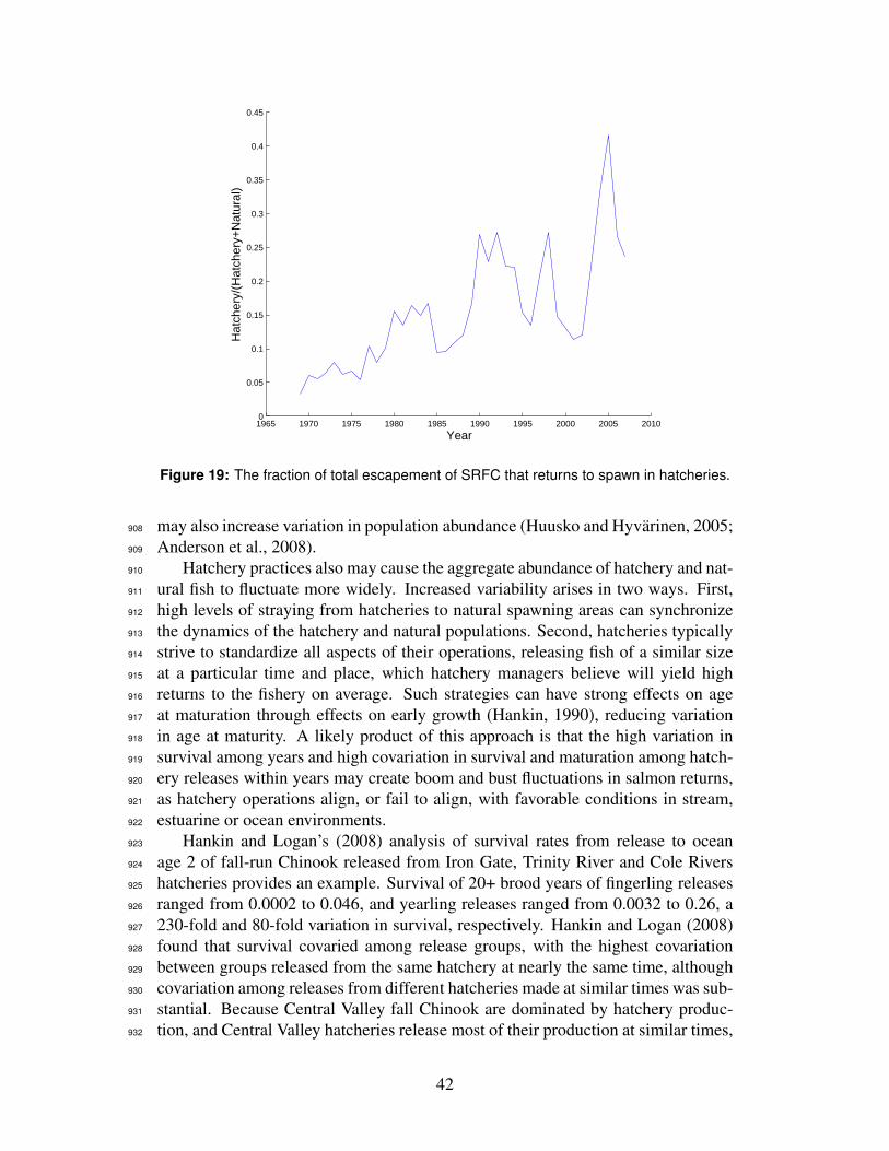
1965 1970 1975 1980 1985 1990 1995 2000 2005 20100

0.05

0.1

0.15

0.2

0.25

0.3

0.35

0.4

0.45

Year

Hat

cher

y/(H

atch

ery+

Nat

ural

)

Figure 19: The fraction of total escapement of SRFC that returns to spawn in hatcheries.

may also increase variation in population abundance (Huusko and Hyvarinen, 2005;908

Anderson et al., 2008).909

Hatchery practices also may cause the aggregate abundance of hatchery and nat-910

ural fish to fluctuate more widely. Increased variability arises in two ways. First,911

high levels of straying from hatcheries to natural spawning areas can synchronize912

the dynamics of the hatchery and natural populations. Second, hatcheries typically913

strive to standardize all aspects of their operations, releasing fish of a similar size914

at a particular time and place, which hatchery managers believe will yield high915

returns to the fishery on average. Such strategies can have strong effects on age916

at maturation through effects on early growth (Hankin, 1990), reducing variation917

in age at maturity. A likely product of this approach is that the high variation in918

survival among years and high covariation in survival and maturation among hatch-919

ery releases within years may create boom and bust fluctuations in salmon returns,920

as hatchery operations align, or fail to align, with favorable conditions in stream,921

estuarine or ocean environments.922

Hankin and Logan’s (2008) analysis of survival rates from release to ocean923

age 2 of fall-run Chinook released from Iron Gate, Trinity River and Cole Rivers924

hatcheries provides an example. Survival of 20+ brood years of fingerling releases925

ranged from 0.0002 to 0.046, and yearling releases ranged from 0.0032 to 0.26, a926

230-fold and 80-fold variation in survival, respectively. Hankin and Logan (2008)927

found that survival covaried among release groups, with the highest covariation928

between groups released from the same hatchery at nearly the same time, although929

covariation among releases from different hatcheries made at similar times was sub-930

stantial. Because Central Valley fall Chinook are dominated by hatchery produc-931

tion, and Central Valley hatcheries release most of their production at similar times,932

42

this finding is significant: very high variation in ocean abundance and escapement933

should be expected from the system as currently operated.934

A similar mechanism has been proposed to explain the collapse of coho salmon935

fisheries along the Oregon coast following the 1976 ocean regime shift. Cumulative936

habitat loss, overharvest, and the gradual replacement of diverse wild populations937

and life histories with a few hatchery stocks left coho salmon vulnerable to col-938

lapse when ocean conditions suddenly changed (Lawson, 1993; Lichatowich, 1999;939

Williams, 2006b)). The situation is analogous to managing a financial portfolio: a940

well-diversified portfolio will be buffeted less by fluctuating market conditions than941

one concentrated on just a few stocks; the SRFC seems to be quite concentrated in-942

deed.943

4.2 Other Chinook stocks in the Central Valley944

Sacramento River fall Chinook have been the most abundant stock of Chinook945

salmon off of central California in recent decades, but this has not always been946

the case. Sacramento River winter Chinook, late-fall Chinook and especially spring947

Chinook once dominated the production of Chinook from the Central Valley (Fisher,948

1994), but over the decades have dwindled to a few remnant populations mostly949

now under the protection of the Endangered Species Act (Lindley et al., 2004). The950

causes for these declines are the same as those that have affected fall Chinook, but951

because these other stocks spend some portion of their life in freshwater during952

the summer, they have been more strongly impacted by impassable dams that limit953

access to cold-water habitats.954

Spring-run Chinook were once the most abundant of the Central Valley runs,955

with large populations in snow-melt and spring-fed streams in the Sierra Nevada956

and southern Cascades, respectively (Fisher, 1994). Spring-run Chinook have been957

reduced from perhaps 18 major populations spawning in four distinct ecoregions958

within the Central Valley to three remnant populations inhabiting a single ecoregion959

(Lindley et al., 2007). Winter-run Chinook were less abundant than spring Chinook,960

spawning in summer months in a few spring-fed tributaries to the upper Sacramento961

River. Perhaps four distinct populations of winter Chinook have been extirpated962

from their historical spawning grounds, with survivors founding a population in the963

tailwaters of Shasta Dam (Lindley et al., 2004). The historical distribution of late-964

fall-run Chinook is less clear, but their life history requires cool water in summer,965

and thus their distribution has probably also been seriously truncated by impassable966

dams at low elevations in the larger tributaries.967

An examination of the population dynamics of extant Central Valley Chinook968

populations illustrates that if spring, winter and late-fall Chinook contributed sig-969

nificantly to the fishery, the aggregate abundance of Chinook in central California970

waters would be less variable. Populations of Central Valley fall-run Chinook ex-971

hibited remarkably similar dynamics over the past two decades, while other runs972

of Central Valley Chinook did not (Fig. 20 and 21). Almost all fall Chinook popu-973

lations reached peak abundances around 2002, and have all been declining rapidly974

since then. In contrast, late-fall, winter and naturally-spawning spring Chinook975

43

populations have been increasing in abundance over the past decade, although es-976

capement in 2007 was down in some of them and the growth of these populations977

through the 1990s and 2000s has to some extent been driven by habitat restoration978

efforts. This begs the question of why have these other stocks responded differently979

to recent environmental variation.980

The answer may have two parts. One part has to do with hatcheries. As dis-981

cussed above, hatcheries may be increasing the covariation of fall Chinook popu-982

lations by erasing genetic differences among populations that might have caused983

the populations to respond differently to environmental variation. They may be fur-984

ther synchronizing the demographics of the naturally-spawning populations through985

straying of hatchery fish into natural spawning areas, a problem exacerbated by out-986

planting fish to the Delta and bays. Finally, hatchery practices minimize variation987

in size, condition and migration timing, which should tend to increase variation in988

survival rates because “bet hedging” is minimized.989

The other part of the answer may lie in the observation that the other runs of990

Chinook have life history tactics that differ in important ways from fall Chinook.991

While named according to the time of year that adults enter freshwater, each run992

type of Central Valley Chinook has a characteristic pattern of habitat use across993

space and time that leads to differences in the time and size of ocean entry. For994

example, spring-run Chinook juveniles enter the ocean at a broader range of ages995

(with a portion of some populations migrating as yearlings) than fall Chinook, due996

to their use of higher elevations and colder waters. Winter run Chinook spawn in997

summer, and the juveniles enter the ocean at a larger size than fall Chinook, due998

to their earlier emergence and longer period of freshwater residency. Late-fall-run999

Chinook enter freshwater in the early winter, and spawn immediately, but juveniles1000

migrate as yearlings the following winter. Thus, if ocean conditions at the time1001

of ocean entry are critical to the survival of juvenile salmon, we should expect1002

that populations from different runs should respond differently to changing ocean1003

conditions because they enter the ocean at different times and at different sizes.1004

In conclusion, the development of the Sacramento-San Joaquin watershed has1005

greatly simplified and truncated the once-diverse habitats that historically supported1006

a highly diverse assemblage of populations. The life history diversity of this histor-1007

ical assemblage would have buffered the overall abundance of Chinook salmon in1008

the Central Valley under varying climate conditions. We are now left with a fish-1009

ery that is supported largely by four hatcheries that produce mostly fall Chinook1010

salmon. Because the survival of fall Chinook salmon hatchery release groups is1011

highly correlated among nearby hatcheries, and highly variable among years, we1012

can expect to see more booms and busts in this fishery in the future in response1013

to variation in the ocean environment. Simply increasing the production of fall1014

Chinook salmon from hatcheries as they are currently operated may aggravate this1015

situation by further concentrating production in time and space. Rather, the key to1016

reducing variation in production is increasing the diversity of SRFC. In the follow-1017

ing section, we make some recommendations towards this goal.1018

44

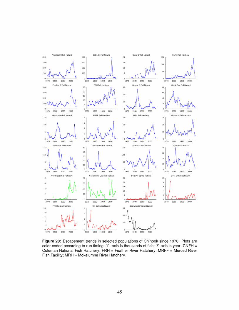
1970 1980 1990 20000

50

100

150

200American R Fall Natural

1970 1980 1990 20000

100

200

300

400Battle Cr Fall Natural

1970 1980 1990 20000

5

10

15

20Clear Cr Fall Natural

1970 1980 1990 20000

50

100

150CNFH Fall Hatchery

1970 1980 1990 20000

50

100

150

200Feather R Fall Natural

1970 1980 1990 20000

5

10

15

20

25FRH Fall Hatchery

1970 1980 1990 20000

10

20

30Merced R Fall Natural

1970 1980 1990 20000

20

40

60

80Middle Sac Fall Natural

1970 1980 1990 20000

5

10

15Mokelumne Fall Natural

1970 1980 1990 20000

1

2

3

4MRFF Fall Hatchery

1970 1980 1990 20000

5

10

15MRH Fall Hatchery

1970 1980 1990 20000

10

20

30Nimbus H Fall Hatchery

1970 1980 1990 20000

5

10

15Stanislaus Fall Natural

1970 1980 1990 20000

10

20

30

40

50Tuolumne R Fall Natural

1970 1980 1990 20000

50

100

150Upper Sac Fall Natural

1970 1980 1990 20000

10

20

30

40Yuba R Fall Natural

1970 1980 1990 20000

2

4

6

8CNFH Late Fall Hatchery

1970 1980 1990 20000

10

20

30

40Sacramento Late Fall Natural

1970 1980 1990 20000

5

10

15

20

25Butte Cr Spring Natural

1970 1980 1990 20000

2

4

6

8

10Deer Cr Spring Natural

1970 1980 1990 20000

2

4

6

8

10FRH Spring Hatchery

1970 1980 1990 20000

1

2

3

4Mill Cr Spring Natural

1970 1980 1990 20000

20

40

60Sacramento Winter Natural

Figure 20: Escapement trends in selected populations of Chinook since 1970. Plots arecolor-coded according to run timing. Y - axis is thousands of fish; X-axis is year. CNFH =Coleman National Fish Hatchery; FRH = Feather River Hatchery; MRFF = Merced RiverFish Facility; MRH = Mokelumne River Hatchery.

45

−0.3 −0.2 −0.1 0 0.1 0.2 0.3 0.4 0.5 0.6−0.8

−0.6

−0.4

−0.2

0

0.2

0.4

0.6

Change in log(abundance) per year, 1990−2000

Cha

nge

in lo

g(ab

unda

nce)

per

yea

r, 2

000−

2007

F

S

F

S

F

SF

S

F

S

F

S

F

F

FF

S

F

LF

S

W

F

F

F

F

Figure 21: Escapement trends in the 1990s and 2000s of various populations of Chinook.F = fall Chinook, S = spring Chinook, LF= late fall Chinook, W= winter Chinook. If popu-lations maintained constant growth rates over the 1990-2007 period, they would fall alongthe dashed diagonal line. All populations fall below the diagonal line, showing that growthrates are lower in the 2000s than in the 1990s, and fall Chinook populations have tendedto decline the fastest in the 2000s.

46

5 Recommendations1019

In this section, we offer recommendations in three areas. First, we identify major1020

information gaps that hindered our analysis of the 2004 and 2005 broods. Filling1021

these gaps should lead to a better understanding of the linkages between survival1022

and environmental conditions. Second, we offer some suggestions on how to im-1023

prove the resilience of SRFC and the Central Valley Chinook stock complex. While1024

changes in harvest opportunities are unavoidable given the expected fluctuations in1025

environmental conditions, it is the panel’s opinion that reducing the volatility of1026

abundance, even at the expense of somewhat lower average catches, would benefit1027

the fishing industry and make fishery disasters less likely. Finally, we point out that1028

an ecosystem-based management and ecological risk assessment framework could1029

improve management of Central Valley Chinook stocks by placing harvest man-1030

agement in the broader context of the Central Valley salmon ecosystem, which is1031

strongly influenced by hatchery operations and management of different ecosystem1032

components, including water, habitat and other species.1033

5.1 Knowledge Gaps1034

We are confident in our conclusion that unusual conditions in the coastal ocean in1035

2005 and 2006 caused the poor performance of the 2004 and 2005 broods. Our1036

case could have been strengthened further, however, with certain kinds of informa-1037

tion that are not currently available. Chief among these is the need for constant1038

fractional marking and tagging of hatchery production, and adequate sampling of1039

fish on the natural spawning grounds. Such information would better identify the1040

contribution of hatcheries to the ocean fishery and natural spawning escapement,1041

survival rates of different hatchery release groups, and the likely degree to which1042

hatchery populations are impacting naturally-spawning populations. Central Valley1043

hatcheries have recently started a constant-fractional marking program for fall Chi-1044

nook, and CDFG is currently planning how to improve in-river sampling for mark1045

and tag recovery. These efforts are critical to improved assessment of SRFC in the1046

future.1047

CDFG has also recently begun to determine the age of returns to the river, which1048

will allow stock assessment scientists to produce cohort reconstructions of the nat-1049

ural stocks in addition to hatchery stocks. Cohort reconstructions provide better1050

survival estimates than the method used in this report (releases of tagged juvenile1051

and recovery of tagged fish at age-two in recreational fisheries) because they are1052

based on many more tag recoveries and provide estimates of fishery mortality and1053

maturation rates.1054

In the case of the 2004 and 2005 broods, freshwater factors did not appear to be1055

the direct cause of the collapse, but future collapses may have multiple contribut-1056

ing causes of similar importance. In such cases, it would be extremely valuable to1057

have reach-specific survival rates like those routinely available for several salmonid1058

species in the Columbia River and recently available for late-fall Chinook and steel-1059

head in the Sacramento River. This would provide powerful and direct information1060

47

about when and where exceptional mortality occurs.1061

Observations of growth and energetic condition of Chinook in the estuary and1062

ocean provided valuable evidence for the 2004 brood, but were unavailable for the1063

2005 and later broods, due to funding limitations.1064

5.2 Improving resilience1065

It appears that the abundance of SRFC is becoming increasingly variable (Fig. 17).1066

Exceptionally high abundance of SRFC may not seem like a serious problem (al-1067

though it does create some problems), but exceptionally low abundances are treated1068

as a crisis. The panel is concerned that such crises are to be expected at a frequency1069

much higher than is acceptable, and that this frequency may be increasing with1070

time due to changes in the freshwater environment, the ocean environment, and the1071

SRFC stock itself. The main hope of reducing this volatility is increasing the diver-1072

sity within and among the populations of fall Chinook in the Central Valley. There1073

are a number of ways to increase diversity.1074

Perhaps the most tractable area for increasing diversity is in changing hatchery1075

operations. We recommend that a hatchery science review panel, be formed to1076

review hatchery practices in the Central Valley. The panel should address a number1077

of questions, including the following:1078

1. assess impacts of outplanting and broodstock transfers among hatcheries on1079

straying and population structure and evaluate alternative release strategies1080

2. evaluate alternative rearing strategies to increase variation in timing of out-1081

migration and age at maturity1082

3. assess whether production levels are appropriate and if they could be adjusted1083

according to expected ocean conditions1084

Ongoing efforts to recover listed Chinook ESUs and increase natural production1085

of anadromous fish in the Central Valley (e.g., the fisheries programs of the Central1086

Valley Project Improvement Act) are also relevant to the problem and should be1087

supported. In particular, efforts to increase the quantity and diversity of spawning1088

and rearing habitats for fall Chinook are likely to be effective in increasing the1089

diversity of life history tactics in that stock.1090

The PFMC should consider creating specific conservation objectives for natural1091

populations of SRFC. Especially in coordination with revised hatchery operations1092

and habitat restoration, managing for natural production could increase diversity1093

within Central Valley fall Chinook. Because conditions for reproduction and juve-1094

nile growth are more variable within and among streams than hatcheries, natural1095

production can be expected to generate a broader range of outmigration and age-at-1096

maturity timings. If straying from hatcheries to natural areas is greatly reduced, the1097

population dynamics of natural populations would be less similar to the dynamics of1098

the hatchery populations, which would smooth the variation of the stock aggregate.1099

48

5.3 Synthesis1100

Addressing hatcheries, habitat and harvest independently would provide benefits1101

to Central Valley Chinook, but addressing them together within a holistic frame-1102

work is likely to be much more successful. The fisheries management community1103

is increasingly recognizing the need to move towards an ecosystem based manage-1104

ment approach. While there is still much uncertainty about what this should en-1105

tail, the ecosystem-based management and ecological risk assessment (EBM/ERA)1106

approach used by the south Florida restoration program (e.g., Harwell et al., 1996;1107

Gentile et al., 2001) is readily applicable to management of Central Valley Chinook.1108

That approach could lead stakeholders to a common view of the different problems1109

afflicting Central Valley Chinook, identify and organize the information needed1110

to effectively manage the ecosystem, better connect this information to decision-1111

making, and reduce the uncertainty surrounding our decisions.1112

At the core of the EBM/ERA approach are conceptual models of how the sys-1113

tem works. The current fishery management regime for SRFC has some features1114

of adaptive management, in that there are clearly stated goals and objectives for1115

the fisheries, monitoring and evaluation programs, and an analytic framework for1116

connecting the data to decisions about operation of the fishery. If one were to make1117

explicit the conceptual model underlying SRFC harvest management, it would in-1118

clude hatcheries that maintain a roughly constant output of fish coupled with ocean1119

and in-river fisheries operating on aggregate stock abundance. The goal is to max-1120

imize harvest opportunities in the current year within constraints posed by vari-1121

ous weak stocks, which do not include naturally-spawning populations of SRFC.1122

The panel feels that it would be useful to expand this conceptual model to include1123

naturally-spawning populations, revised hatchery operations, habitat effects, ocean1124

effects, and climate change. Also, resource managers might consider changing the1125

goal of management from maximizing harvest opportunity for the current year to1126

reducing fluctuations in opportunity from year to year and maintaining the stability1127

of the system for the long term. Both of these goals require viable and productive1128

populations of wild salmon. Not all of the factors in the revised system would be1129

subject to control by fisheries managers, but including them in the model would1130

at least make clear the contribution of these factors to the problem of effectively1131

managing Chinook salmon fisheries.1132

The panel is well aware that the resource management institutions are not well-1133

equipped to pursue this approach, and that many of the actions that could improve1134

the status and resilience of Central Valley Chinook are beyond the authority of the1135

PFMC or any other single agency or entity. Nonetheless, significantly improv-1136

ing the resilience of Central Valley Chinook and the sustainability of California’s1137

Chinook salmon fishery will require resource managers and stakeholders to work1138

together, and EBM/ERA offers a framework for facilitating such cooperation.1139

49

References1140

Anderson, C. N. K., C. H. Hsieh, S. A. Sandin, R. Hewitt, A. Hollowed, J. Bed-1141

dington, R. M. May, and G. Sugihara. 2008. Why fishing magnifies fluctuations1142

in fish abundance. Nature 452:835–839.1143

Barber, R. T. and R. L. Smith. 1981. Coastal upwelling ecosystems. In Analysis1144

of marine ecosystems, A. R. Longhurst, editor, pages 31–68. Academic Press,1145

London.1146

Barnett-Johnson, R., C. B. Grimes, C. F. Royer, and C. J. Donohoe. 2007b. Iden-1147

tifying the contribution of wild and hatchery Chinook salmon (Oncorhynchus1148

tshawytscha) to the ocean fishery using otolith microstructure as natural tags.1149

Canadian Journal of Fisheries and Aquatic Sciences 64:1683–1692.1150

Beamish, R. J., D. J. Noakes, G. A. McFarlane, L. Klyashtorin, V. V. Ivanov, and1151

V. Kurashov. 1999. The regime concept and natural trends in the production of1152

Pacific salmon. Can. J. Fish. Aquat. Sci. 56:516–526.1153

Bisson, P. A., C. C. Coutant, D. Goodman, R. Gramling, D. Lettenmaier, J. Licha-1154

towich, W. Liss, E. Loudenslager, L. McDonald, D. Philipp, and B. Riddell. 2002.1155

Hatchery surpluses in the Pacific Northwest. Fisheries 27:16–27.1156

Botsford, L. W. and C. A. Lawrence. 2002. Patterns of co-variability among Califor-1157

nia Current chinook salmon, coho salmon, Dungeness crab, and physical oceano-1158

graphic conditions. Progress In Oceanography 53:283–305.1159

Bottom, D. L., K. K. Jones, T. J. Cornwell, A. Gray, and C. A. Simenstad. 2005a.1160

Patterns of Chinook salmon emigration and residency in the Salmon River estu-1161

ary (Oregon). Estuarine Coastal and Shelf Science 64:79–93.1162

Bottom, D. L., C. A. Simenstad, J. Burke, A. M. Baptista, D. A. Jay, K. K.1163

Jones, E. Casillas, and M. H. Schiewe. 2005b. Salmon at river’s end: the role1164

of the estuary in the decline and recovery of Columbia River salmon. NOAA1165

Tech. Memo. NMFS-NWFSC-68, U.S. Dept. Commer.1166

Brodeur, R. D., J. P. Fisher, D. J. Teel, R. L. Emmett, E. Casillas, and T. W. Miller.1167

2004. Juvenile salmonid distribution, growth, condition, origin, and environmen-1168

tal and species associations in the Northern California Current. Fishery Bulletin1169

102:25–46.1170

Brodeur, R. D., S. Ralston, R. L. Emmett, M. Trudel, T. D. Auth, and A. J. Phillips.1171

2006. Anomalous pelagic nekton abundance, distribution, and apparent recruit-1172

ment in the northern California Current in 2004 and 2005. Geophysical Research1173

Letters 33:L22S08.1174

Budy, P., G. P. Thiede, N. Bouwes, C. E. Petrosky, and H. Schaller. 2002. Evidence1175

linking delayed mortality of Snake River salmon to their earlier hydrosystem1176

experience. North American Journal of Fisheries Management 22:35–51.1177

50

CDFG (California Department of Fish and Game). 2008. Focus areas of research1178

relative to the status of the 2004 and 2005 broods of the Central Valley fall Chi-1179

nook salmon stock. Pacific Fishery Management Council.1180

CDFG and NMFS(California Department of Fish and Game and National Marine1181

Fisheries Service). 2001. Final report on anadromous salmonid fish hatcheries1182

in California. Technical report, California Department of Fish and Game and1183

National Marine Fisheries Service Southwest Region.1184

Christensen, J., B. Hewitson, A. Busuioc, A. Chen, X. Gao, I. Held, R. Jones,1185

R. K. Kolli, W. T. Kwon, R. Laprise, V. Magana Rueda, L. Mearns, C. Men-1186

ndez, J. Raisanen, A. Rinke, S. A., and P. Whetton. 2007. Regional climate1187

projections. In Climate Change 2007: The Physical Science Basis. Contribution1188

of Working Group I to the Fourth Assessment Report of the Intergovernmental1189

Panel on Climate Change, S. Solomon, D. Qin, M. Manning, Z. Chen, M. Mar-1190

quis, K. Averyt, M. Tignor, and H. Miller, editors. Cambridge University Press,1191

Cambridge, United Kingdom and New York, NY, USA.1192

Darimont, C. T., S. M. Carlson, M. T. Kinnison, P. C. Paquet, T. E. Reimchen, and1193

C. C. Wilmers. 2009. Human predators outpace other agents of trait change in1194

the wild. Proceedings of the National Academy of Sciences of the United States1195

of America 106:952–954.1196

Dever, E. P., C. E. Dorman, and J. L. Largier. 2006. Surface boundary-layer vari-1197

ability off Northern California, USA, during upwelling. Deep Sea Research Part1198

II: Topical Studies in Oceanography 53:2887–2905.1199

Fisher, F. W. 1994. Past and present status of Central Valley chinook salmon. Con-1200

servation Biology 8:870–873.1201

Fisher, J. P., M. Trudel, A. Ammann, J. A. Orsi, J. Piccolo, C. Bucher, E. Casillas,1202

J. A. Harding, R. B. MacFarlane, R. D. Brodeur, J. F. T. Morris, and D. W. Welch.1203

2007. Comparisons of the coastal distributions and abundances of juvenile Pacific1204

salmon from central California to the northern Gulf of Alaska. In The ecology1205

of juvenile salmon in the northeast Pacific Ocean: regional comparisons, C. B.1206

Grimes, R. D. Brodeur, L. J. Haldorson, and S. M. McKinnell, editors, pages1207

31–80. American Fisheries Society, Bethesda, MD.1208

Gargett, A. E. 1997. The optimal stability ‘window’: a mechanism underlying1209

decadal fluctuations in North Pacific salmon stocks? Fisheries Oceanography1210

6:109–117.1211

Gentile, J. H., M. A. Harwell, W. Cropper, C. C. Harwell, D. DeAngelis, S. Davis,1212

J. C. Ogden, and D. Lirman. 2001. Ecological conceptual models: a framework1213

and case study on ecosystem management for South Florida sustainability. Sci-1214

ence of the Total Environment 274:231–253.1215

51

Good, T. P., R. S. Waples, and P. Adams. 2005. Updated status of federally listed1216

ESUs of west coast salmon and steelhead. NOAA Tech. Memo. NMFS-NWFSC-1217

66, U.S. Dept. Commer.1218

Hankin, D. G. 1990. Effects of month of release of hatchery-reared chinook salmon1219

on size at age, maturation schedule, and fishery contribution. Information Reports1220

Number 90-4, Fish Division, Oregon Department of Fish and Wildlife.1221

Hankin, D. G. and E. Logan. 2008. A preliminary analysis of chinook salmon1222

coded-wire tag recovery data from Iron Gate, Trinity River and Cole Rivers1223

hatcheries, brood years 1978-2001. Review draft.1224

Hard, J. J., M. R. Gross, M. Heino, R. Hilborn, R. G. Kope, R. Law, and J. D.1225

Reynolds. 2008. Evolutionary consequences of fishing and their implications for1226

salmon. Evolutionary Applications 1:388–408.1227

Hare, S. R. and R. C. Francis. 1995. Climate change and salmon production in1228

the Northeast Pacific Ocean. In Climate Change and Northern Fish Popula-1229

tions. Canadian Special Publications in Fisheries and Aquatic Sciences 121, R. J.1230

Beamish, editor, pages 357–372.1231

Harwell, M. A., J. F. Long, A. M. Bartuska, J. H. Gentile, C. C. Harwell, V. Myers,1232

and J. C. Ogden. 1996. Ecosystem management to achieve ecological sustain-1233

ability: The case of south Florida. Environmental Management 20:497–521.1234

Healey, M. C. 1991. Life history of chinook salmon (Oncorhynchus tswawytscha).1235

In Pacific salmon life histories, C. Margolis and L. Groot, editors, pages 311–1236

394. University of British Columbia Press, Vancouver.1237

Hilborn, R., T. P. Quinn, D. E. Schindler, and D. E. Rogers. 2003. Biocomplexity1238

and fisheries sustainability. Proceedings of the National Academy of Sciences,1239

USA 100:6564–6568.1240

Hobday, A. J. and G. W. Boehlert. 2001. The role of coastal ocean variation in1241

spatial and temporal patterns in survival and size of coho salmon (Oncorhynchus1242

kisutch). Canadian Journal of Fisheries and Aquatic Sciences 58:2021–2036.1243

Hooff, R. C. and W. T. Peterson. 2006. Copepod biodiversity as an indicator1244

of changes in ocean and climate conditions of the northern California current1245

ecosystem. Limnology and Oceanography 51:2607–2620.1246

Houde, E. D. 1975. Effects of stocking density and food density on survival, growth1247

and yield of laboratory-reared larvae of sea bream Archosargus rhomboidalis (L.)1248

(Sparidae). Journal of Fish Biology 7:115–127.1249

Huusko, A. and P. Hyvarinen. 2005. A high harvest rate induces a tendency to1250

generation cycling in a freshwater fish population. Journal of Animal Ecology1251

74:525–531.1252

52

ISAB (Independent Scientific Advisory Board). 2007. Latent mortality report: re-1253

view of hypotheses and causative factors contributing to latent mortality and their1254

likely relevenace to he ”below Bonneville” component of the COMPASS model.1255

ISAB 2007-1. ISAB, Portland, OR.1256

Ingraham, J. W. J. and R. K. Miyahara. 1988. Ocean surface current simulations in1257

the North Pacific Ocean and Bering Sea (OSCURS – Numerical Models). NOAA1258

Tech. Memo. NMFS F/NWC-130, U.S. Dept. Commer.1259

Jeffres, C. A., J. J. Opperman, and P. B. Moyle. 2008. Ephemeral floodplain habitats1260

provide best growth conditions for juvenile Chinook salmon in a California river.1261

Environmental Biology of Fishes 83:449–458.1262

Kjelson, M. A. and P. L. Brandes. 1989. The use of smolt survival estimates to1263

quantify the effects of habitat changes on salmonid stocks in the Sacramento-1264

San Joaquin rivers, California. In Proceedings of the National Workshop on the1265

effects of habitat alteration on salmonid stocks, C. D. Levings, L. B. Holtby,1266

and M. A. Henderson, editors, Canadian Special Publications in Fisheries and1267

Aquatic Sciences, volume 105, pages 100–115.1268

Kope, R. G. and L. W. Botsford. 1990. Determination of factors affecting recruit-1269

ment of chinook salmon Oncorhynchus tshawytscha in central California. Fish-1270

ery Bulletin 88:257–269.1271

Kruse, G. H. 1998. Salmon run failures in 1997–1998: a link to anomalous ocean1272

conditions? Alaska Fishery Research Bulletin 5:55–63.1273

Lawson, P. W. 1993. Cycles in ocean productivity, trends in habitat quality, and the1274

restoration of salmon runs in Oregon. Fisheries 18:6–10.1275

Lawson, P. W., E. A. Logerwell, N. J. Mantua, R. C. Francis, and V. N. Agostini.1276

2004. Environmental factors influencing freshwater survival and smolt produc-1277

tion in Pacific Northwest coho salmon (Oncorhynchus kisutch). Canadian Journal1278

of Fisheries and Aquatic Sciences 61:360–373.1279

Lichatowich, J. 1999. Salmon without rivers: a history of the Pacific salmon crisis.1280

Island Press, Washington, DC.1281

Lindley, S. T., R. S. Schick, B. May, J. J. Anderson, S. Greene, C. Hanson,1282

A. Low, D. McEwan, R. B. MacFarlane, C. Swanson, and J. G. Williams.1283

2004. Population structure of threatened and endangered chinook salmon ESUs1284

in California’s Central Valley basin. NOAA Tech. Memo. NMFS-SWFSC-360,1285

U.S. Dept. Commer.1286

Lindley, S. T., R. S. Schick, E. Mora, P. B. Adams, J. J. Anderson, S. Greene,1287

C. Hanson, B. P. May, D. McEwan, R. B. MacFarlane, C. Swanson, and J. G.1288

Williams. 2007. Framework for assessing viability of threatened and endangered1289

Chinook salmon and steelhead in the Sacramento-San Joaquin basin. San Fran-1290

cisco Estuary and Watershed Science 5(1):Article 4.1291

53

MacFarlane, R. B. and E. C. Norton. 2002. Physiological ecology of juvenile chi-1292

nook salmon (Oncorhynchus tshawytscha) at the southern end of their distribu-1293

tion, the San Francisco Estuary and Gulf of the Farallones, California. Fishery1294

Bulletin 100:244–257.1295

Mantua, N., S. Hare, Y. Zhang, J. Wallace, and R. Francis. 1997. A Pacific inter-1296

decadal climate oscillation with impacts on salmon production. Bulletin of the1297

American Meteorological Society 78:1069–1079.1298

MBARI (Monterey Bay Aquarium Research Institute). 2006. Annual report.1299

MBARI, Moss Landing, CA.1300

McCullough, D. A. 1999. A review and synthesis of effects of alteration to the1301

water temperature regime on freshwater life stages of salmonids, with special1302

reference to chinook salmon. Document 910-R-99010, United States Environ-1303

mental Protection Agency. Seattle, WA.1304

McEvoy, A. F. 1986. The fisherman’s problem: ecology and law in the California1305

fisheries. Cambridge University Press, New York, New York.1306

McIsaac, D. O. 2008. Pacific Fishery Management Council request for scientific1307

review of factors affecting certain west coast salmon stocks. Supplemental Infor-1308

mational Report 5, Pacific Fishery Management Council. Portland, OR.1309

Mueter, F. J., R. M. Peterman, and B. J. Pyper. 2002. Opposite effects of ocean1310

temperature on survival rates of 120 stocks of Pacific salmon (Oncorhynchus1311

spp.) in northern and southern areas. Canadian Journal of Fisheries and Aquatic1312

Sciences 59:456–463.1313

Myers, J. M., R. G. Kope, G. J. Bryant, D. Teel, L. J. Lierheimer, T. C. Wainwright,1314

W. S. Grant, F. W. Waknitz, K. Neely, S. T. Lindley, and R. S. Waples. 1998. Sta-1315

tus review of chinook salmon from Washington, Idaho, Oregon, and California.1316

NOAA Tech. Memo. NMFS-NWFSC-35, U.S. Dept. Commer.1317

Newell, C. L. and T. J. Cowles. 2006. Unusual gray whale Eschrichtius robus-1318

tus feeding in the summer of 2005 off the central Oregon Coast. Geophysical1319

Research Letters 33:L22S11.1320

Newman, K. B. and J. Rice. 2002. Modeling the survival of chinook salmon smolts1321

outmigrating through the lower Sacramento River system. Journal of the Ameri-1322

can Statistical Association 97:983–993.1323

O’Farrell, M. R., M. S. Mohr, M. L. Palmer-Zwahlen, and A. M. Grover. 2009. The1324

Sacramento Index. Report in preparation.1325

Pearcy, W. G. 1992. Ocean ecology of North Pacific salmonids. University of1326

Washinton, Seattle, WA.1327

54

PFMC (Pacific Fishery Management Council). 2007. Preseason report III: Anal-1328

ysis of council adopted management measures for 2007 ocean salmon fisheries.1329

Pacific Fishery Management Council, 7700 NE Ambassador Place, Suite 101,1330

Portland, Oregon 97220-1384.1331

PFMC (Pacific Fishery Management Council). 2008. Preseason report I: Stock1332

abundance analysis for 2008 ocean salmon fisheries. Pacific Fishery Management1333

Council, 7700 NE Ambassador Place, Suite 101, Portland, Oregon 97220-1384.1334

PFMC (Pacific Fishery Management Council). 2009. Review of 2008 ocean salmon1335

fisheries. Pacific Fishery Management Council, 7700 NE Ambassador Place,1336

Suite 101, Portland, Oregon 97220-1384.1337

Pyper, B. J., F. J. Mueter, R. M. Peterman, D. J. Blackbourn, and C. C. Wood.1338

2002. Spatial covariation in survival rates of Northeast Pacific chum salmon.1339

Transactions of the American Fisheries Society 131:343–363.1340

Reisenbichler, R. R. and S. P. Rubin. 1999. Genetic changes from artificial prop-1341

agation of Pacific salmon affect the productivity and viability of supplemented1342

populations. ICES Journal of Marine Science 56:459–466.1343

Rykaczewski, R. R. and D. J. Checkley. 2008. Influence of ocean winds on the1344

pelagic ecosystem in upwelling regimes. Proceedings of the National Academy1345

of Sciences 105:1967–1970.1346

Ryther, J. H. 1969. Photosynthesis and fish production in the sea. Science 166:72–1347

76.1348

Schwing, F. B., N. A. Bond, S. J. Bograd, T. Mitchell, M. A. Alexander, and1349

N. Mantua. 2006. Delayed coastal upwelling along the US West Coast in 2005:1350

A historical perspective. Geophysical Research Letters 33:L22S01.1351

Schwing, F. B., T. Murphree, and P. M. Green. 2002. The Northern Oscillation1352

Index (NOI): a new climate index for the northeast Pacific. Progress In Oceanog-1353

raphy 53:115–139.1354

Sommer, T. R., M. L. Nobriga, W. C. Harrel, W. Batham, and W. J. Kimmerer. 2001.1355

Floodplain rearing of juvenile chinook salmon: evidence of enhanced growth and1356

survival. Can. J. Fish. Aquat. Sci. 58:325–333.1357

SRFCRT (Sacramento River Fall Chinook Review Team). 1994. Sacramento River1358

Fall Chinook Review Team: An assessment of the status of the Sacramento River1359

fall chinook stiock as required under the salmon fishery management plan. Pacific1360

Fishery Management Council.1361

Sydeman, W. J., R. W. Bradley, P. Warzybok, C. L. Abraham, J. Jahncke, K. D.1362

Hyrenbach, V. Kousky, J. M. Hipfner, and M. D. Ohman. 2006. Planktivorous1363

auklet Ptychoramphus aleuticus responses to ocean climate, 2005: Unusual at-1364

mospheric blocking? Geophysical Research Letters 33:L22S09.1365

55

Vogel, D. A. and K. R. Marine. 1991. Guide to upper Sacramento chinook salmon1366

life history. CH2M Hill.1367

Weise, M. J., D. P. Costa, and R. M. Kudela. 2006. Movement and diving behavior1368

of male California sea lion (Zalophus californianus) during anomalous oceano-1369

graphic conditions of 2005 compared to those of 2004. Geophysical Research1370

Letters 33:L22S10.1371

Weitkamp, L. A. In review. Marine distributions of Chinook salmon (Oncorhynchus1372

tshawytscha) from the west coast of North America determined by coded wire tag1373

recoveries.1374

Welch, D. W., E. L. Rechisky, M. C. Melnychuk, A. D. Porter, C. J. Walters,1375

S. Clements, B. J. Clemens, R. S. McKinley, and C. Schreck. 2008. Survival1376

of migrating salmon smolts in large rivers with and without dams. PLoS Biology1377

6:2101–2108.1378

Wells, B. K., J. C. Field, J. A. Thayer, C. B. Grimes, S. J. Bograd, W. J. Sydeman,1379

F. B. Schwing, and R. Hewitt. 2008. Untangling the relationships among climate,1380

prey and top predators in an ocean ecosystem. Marine Ecology Progress Series1381

364:15–29.1382

Wilkerson, F. P., A. M. Lassiter, R. C. Dugdale, A. Marchi, and V. E. Hogue. 2006.1383

The phytoplankton bloom response to wind events and upwelled nutrients during1384

the CoOP WEST study. Deep Sea Research Part II: Topical Studies in Oceanog-1385

raphy 53:3023–3048.1386

Williams, J. G. 2006a. Central Valley salmon: a perspective on Chinook and steel-1387

head in the Central Valley of California. San Francisco Estuary and Watershed1388

Science 4(3):Article 2.1389

Williams, J. G., S. G. Smith, and W. D. Muir. 2001. Survival estimates for down-1390

stream migrant yearling juvenile salmonids through the Snake and Columbia1391

rivers hydropower system, 1966–1980 and 1993–1999. North American Jour-1392

nal of Fisheries Management 21:310–317.1393

Williams, R. N., editor. 2006b. Return to the river: restoring salmon to the1394

Columbia River. Elsevier Academic Press, San Diego, CA.1395

Williamson, K. S. and B. May. 2005. Homogenization of fall-run Chinook salmon1396

gene pools in the Central Valley of California, USA. North American Journal of1397

Fisheries Management 25:993–1009.1398

Wolf, S. G., W. J. Sydeman, J. M. Hipfner, C. L. Abraham, B. R. Tershy, and D. A.1399

Croll. 2009. Range-wide reproductive consequences of ocean climate variability1400

for the seabird Cassins Auklet. Ecology 90:742–753.1401

56

Yoshiyama, R. M., F. W. Fisher, and P. B. Moyle. 1998. Historical abundance1402

and decline of chinook salmon in the Central Valley region of California. North1403

American Journal of Fisheries Management 18:487–521.1404

Yoshiyama, R. M., E. R. Gerstung, F. W. Fisher, and P. B. Moyle. 2001. Historic1405

and present distribution of chinook salmon in the Central Valley drainage of Cal-1406

ifornia. In Fish Bulletin 179: Contributions to the biology of Central Valley1407

salmonids., R. L. Brown, editor, volume 1, pages 71–176. California Department1408

of Fish and Game, Sacramento, CA.1409

57