1

Instrument Science Report WFC3 2009-39

WFC3 SMOV Program 11453:

IR Flat Field Uniformity

B. Hilbert, V. Kozhurina-Platais, E. Sabbi

5 November 2009

ABSTRACT

Using data taken during the 2009 Servicing Mission Observatory Verification (SMOV),

we have analyzed the quality of the Thermal Vacuum 3 (TV3) derived flat fields for the

F110W, F125W, F140W, and F160W filters. These ground-based flats are currently

used in the standard calibration of all WFC3/IR observations. By comparing photometry

results from a set of stars observed on orbit at multiple locations on the detector, we are

able to quantify residual differences in detector response after the application of the TV3

flat fields. We find variations in photometry of up to 1.5% across the detector in all four

filters.

Introduction

After its installation in HST during the May 2009 servicing mission, testing of the

WFC3 cooled IR detector began in mid-June 2009. Program 11453, “IR Flat Field

Uniformity” executed between July 15 and 17, 2009, with the goal of quantifying

differences between flat field images created on the ground before launch versus on-orbit

flats.

During TV3 testing in the spring of 2008, we obtained flat field images through all of

the IR filters using an external optical stimulus (CASTLE) as the illumination source.

CASTLE provided a more uniform pattern of illumination, and higher illumination level

than is possible using the WFC3 Tungsten lamps. These high quality flat fields are

currently used in the WFC3 data reduction pipeline on all WFC3/IR data.

2

However, past experience with ACS (ACS ISR 2002-0008, Mack et al. 2002),

suggests that there could be significant differences between ground testing and on orbit

flat fields. SMOV Program 11543 was developed to collect data suitable for quantifying

any observed differences in WFC3/IR data. By performing the standard data reduction

steps on these data, including the application of the TV3 flat fields, any residual

variations in response across the detector would be the result of a change in the flat field

behavior between TV3 and SMOV.

Data

Data collected include multiple observations of 47 Tucanae (NGC104) taken through

the four IR wide band filters. We used an observing strategy similar to that used by ACS

in past calibration campaigns (ACS ISR 2002-0008, Mack et al. 2002), and to SMOV

Program 11452, which was used to test the WFC3/UVIS flat field uniformity. (WFC3

ISR 2009-19, Sabbi 2009)

All data were obtained in full-frame mode with MEB2, using Science Mission

Specifications (SMS), i.e. no real time commanding. The temperature of the IR detector

was -127.9 C (145.1 K) and constant to within 0.2oC throughout the observations. All

data were obtained at the nominal 2.5 e-/ADU gain setting.

For each of the F110W, F125W, F140W, and F160W filters, we collected two ramps

at each of 9 pointings. The pointings were arranged in a 3x3 box with a shift in the x

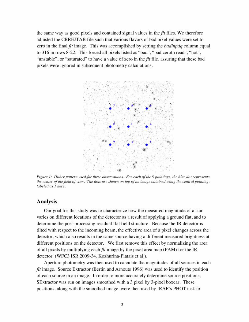
and/or y direction of roughly 20% of the detector’s field of view between each. Figure 1

gives a graphical view of the 9-point dither pattern, with each point denoting the center of

one of the 9 pointings. The star field shown here represents the field of view for only the

central pointing. Table 2 lists all of the data files collected as part of this proposal, along

with relevant details for each.

All data were reduced using CALWF3 version 1.7 for basic data reduction. This

included reference pixel subtraction, zeroth read subtraction, cosmic ray rejection, non-

linearity correction, flat fielding, and conversion to units of electrons per second. Table 3

in Appendix 1 lists the reference files used by CALWF3 for its processing steps. We

made two changes to the default CALWF3 processing steps when running these data

through the pipeline.

First we adjusted the gain values applied to the data. Initial data analysis indicated

that a quadrant-to-quadrant offset in the photometry results was present when the data

were reduced using SMOV-derived gain values. (See Hilbert and McCullough ISR

WFC3 2009-23 for these gain values). When we applied an identical gain to all four

quadrants this quadrant dependence was minimized. We therefore replaced the gain

values in the CCDTAB file (listed in Table 3) with values of 2.4 e-/ADU for all

quadrants.

The second adjustment we made was in the way CALWF3 treated bad pixels. In

version 1.7 of CALWF3, pixels marked as bad in the bad pixel mask were processed in

3

the same way as good pixels and contained signal values in the flt files. We therefore

adjusted the CRREJTAB file such that various flavors of bad pixel values were set to

zero in the final flt image. This was accomplished by setting the badinpdq column equal

to 316 in rows 8-22. This forced all pixels listed as “bad”, “bad zeroth read”, “hot”,

“unstable”, or “saturated” to have a value of zero in the flt file, assuring that these bad

pixels were ignored in subsequent photometry calculations.

Figure 1: Dither pattern used for these observations. For each of the 9 pointings, the blue dot represents

the center of the field of view. The dots are shown on top of an image obtained using the central pointing,

labeled as 1 here.

Analysis

Our goal for this study was to characterize how the measured magnitude of a star

varies on different locations of the detector as a result of applying a ground flat, and to

determine the post-processing residual flat field structure. Because the IR detector is

tilted with respect to the incoming beam, the effective area of a pixel changes across the

detector, which also results in the same source having a different measured brightness at

different positions on the detector. We first remove this effect by normalizing the area

of all pixels by multiplying each flt image by the pixel area map (PAM) for the IR

detector (WFC3 ISR 2009-34, Kozhurina-Platais et al.).

Aperture photometry was then used to calculate the magnitudes of all sources in each

flt image. Source Extractor (Bertin and Arnouts 1996) was used to identify the position

of each source in an image. In order to more accurately determine source positions,

SExtractor was run on images smoothed with a 3 pixel by 3-pixel boxcar. These

positions, along with the smoothed image, were then used by IRAF’s PHOT task to

4

perform initial aperture photometry and further refine the source positions through

Gaussian fitting. Finally, PHOT used the refined positions and the original flt image

(multiplied by the PAM), to perform final aperture photometry on all sources, using a 3-

pixel radius aperture. This photometry procedure is similar to that used in the analysis of

the data used to create the IR PAM (WFC3 ISR 2009-34 Kozhurina-Platais et al.).

For each filter, we combined the photometric catalogs from all pointings using a

triangle matching script and a 4th order polynomial. We then calculated a sigma-clipped

mean magnitude for each star and then subtracted the magnitude of the star measured in

the reference image (position 1 in Figure 1). In order to collect more robust statistics on

these magnitude differences, we limited our sample of stars to those with a signal-to-

noise ratio greater than 16. This resulted in a population of roughly 1100 stars across the

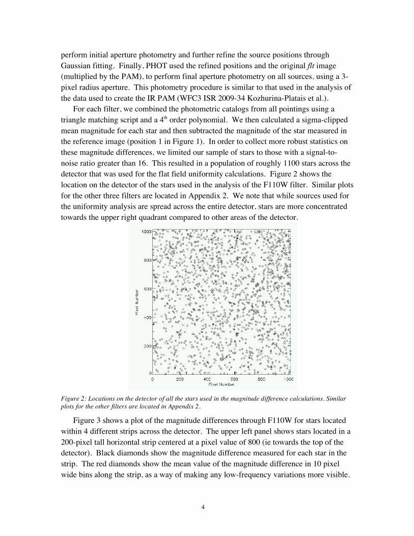
detector that was used for the flat field uniformity calculations. Figure 2 shows the

location on the detector of the stars used in the analysis of the F110W filter. Similar plots

for the other three filters are located in Appendix 2. We note that while sources used for

the uniformity analysis are spread across the entire detector, stars are more concentrated

towards the upper right quadrant compared to other areas of the detector.

Figure 2: Locations on the detector of all the stars used in the magnitude difference calculations. Similar

plots for the other filters are located in Appendix 2.

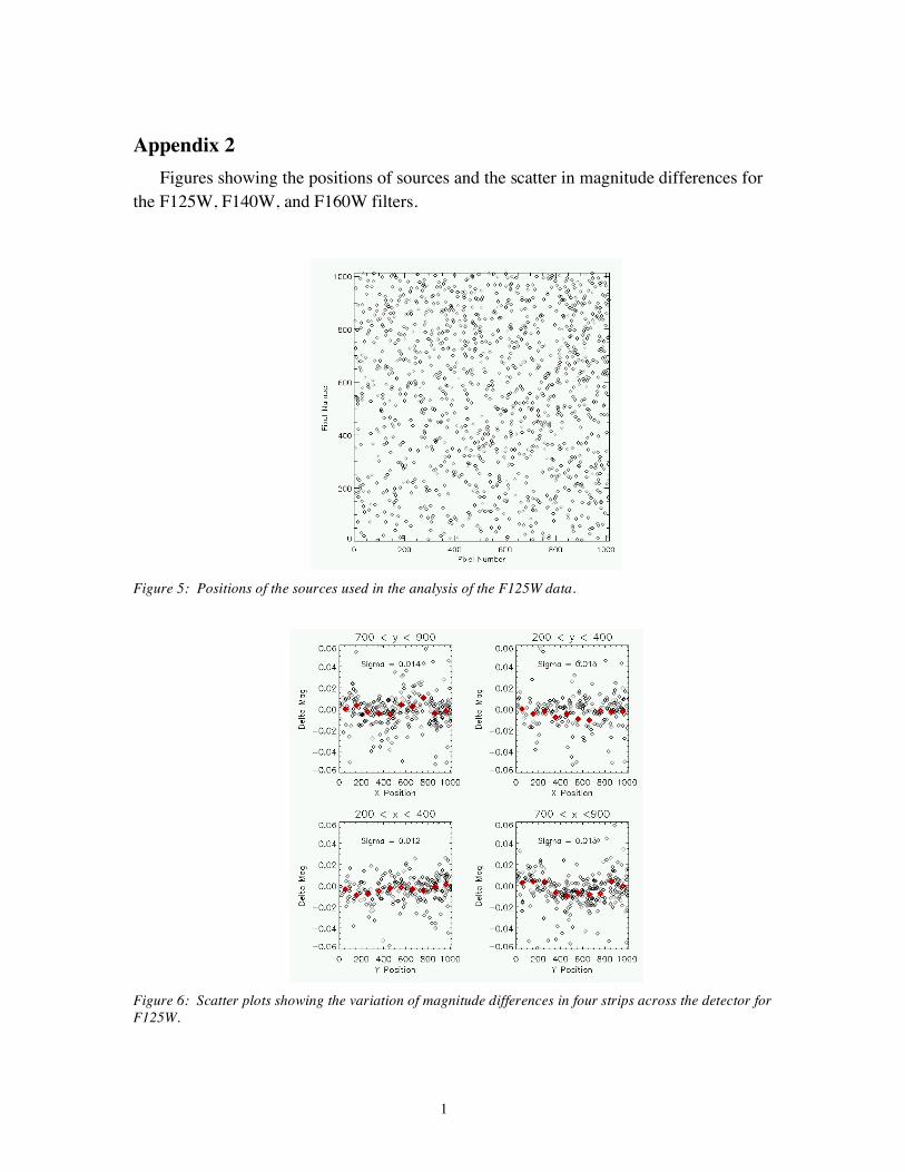
Figure 3 shows a plot of the magnitude differences through F110W for stars located

within 4 different strips across the detector. The upper left panel shows stars located in a

200-pixel tall horizontal strip centered at a pixel value of 800 (ie towards the top of the

detector). Black diamonds show the magnitude difference measured for each star in the

strip. The red diamonds show the mean value of the magnitude difference in 10 pixel

wide bins along the strip, as a way of making any low-frequency variations more visible.

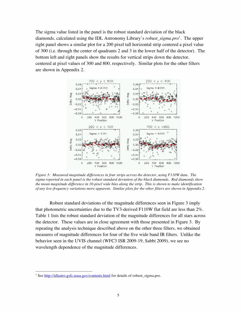
5

The sigma value listed in the panel is the robust standard deviation of the black

diamonds, calculated using the IDL Astronomy Library’s robust_sigma.pro1. The upper

right panel shows a similar plot for a 200 pixel tall horizontal strip centered a pixel value

of 300 (i.e. through the center of quadrants 2 and 3 in the lower half of the detector). The

bottom left and right panels show the results for vertical strips down the detector,

centered at pixel values of 300 and 800, respectively. Similar plots for the other filters

are shown in Appendix 2.

Figure 3: Measured magnitude differences in four strips across the detector, using F110W data. The

sigma reported in each panel is the robust standard deviation of the black diamonds. Red diamonds show

the mean magnitude difference in 10-pixel wide bins along the strip. This is shown to make identification

of any low-frequency variations more apparent. Similar plots for the other filters are shown in Appendix 2.

Robust standard deviations of the magnitude differences seen in Figure 3 imply

that photometric uncertainties due to the TV3-derived F110W flat field are less than 2%.

Table 1 lists the robust standard deviation of the magnitude differences for all stars across

the detector. These values are in close agreement with those presented in Figure 3. By

repeating the analysis technique described above on the other three filters, we obtained

measures of magnitude differences for four of the five wide band IR filters. Unlike the

behavior seen in the UVIS channel (WFC3 ISR 2009-19, Sabbi 2009), we see no

wavelength dependence of the magnitude differences.

1 See http://idlastro.gsfc.nasa.gov/contents.html for details of robust_sigma.pro.

6

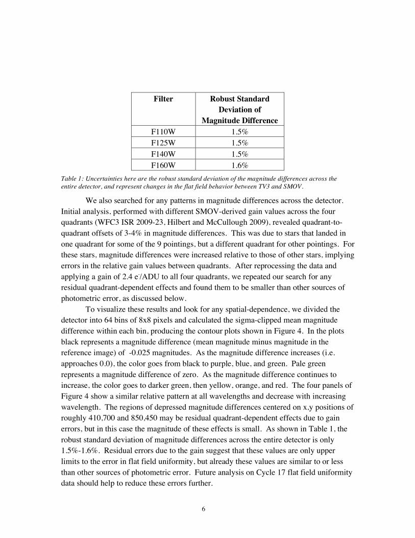
Filter Robust Standard

Deviation of

Magnitude Difference

F110W 1.5%

F125W 1.5%

F140W 1.5%

F160W 1.6%

Table 1: Uncertainties here are the robust standard deviation of the magnitude differences across the

entire detector, and represent changes in the flat field behavior between TV3 and SMOV.

We also searched for any patterns in magnitude differences across the detector.

Initial analysis, performed with different SMOV-derived gain values across the four

quadrants (WFC3 ISR 2009-23, Hilbert and McCullough 2009), revealed quadrant-to-

quadrant offsets of 3-4% in magnitude differences. This was due to stars that landed in

one quadrant for some of the 9 pointings, but a different quadrant for other pointings. For

these stars, magnitude differences were increased relative to those of other stars, implying

errors in the relative gain values between quadrants. After reprocessing the data and

applying a gain of 2.4 e-/ADU to all four quadrants, we repeated our search for any

residual quadrant-dependent effects and found them to be smaller than other sources of

photometric error, as discussed below.

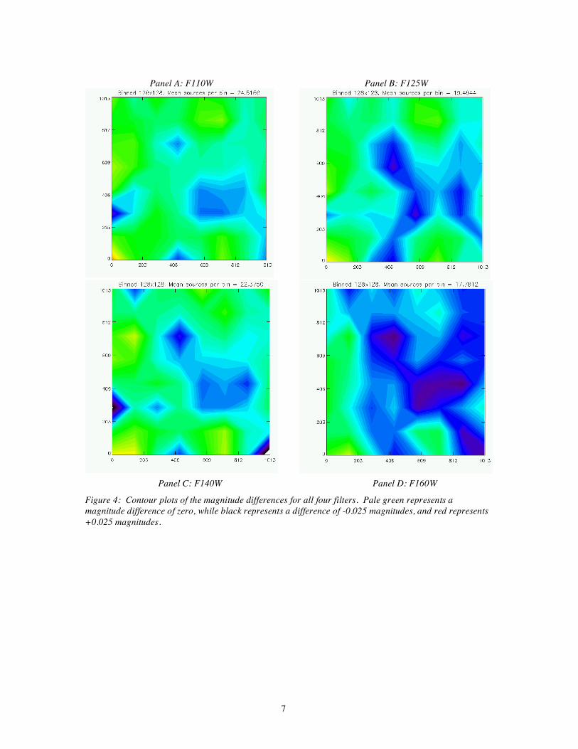
To visualize these results and look for any spatial-dependence, we divided the

detector into 64 bins of 8x8 pixels and calculated the sigma-clipped mean magnitude

difference within each bin, producing the contour plots shown in Figure 4. In the plots

black represents a magnitude difference (mean magnitude minus magnitude in the

reference image) of -0.025 magnitudes. As the magnitude difference increases (i.e.

approaches 0.0), the color goes from black to purple, blue, and green. Pale green

represents a magnitude difference of zero. As the magnitude difference continues to

increase, the color goes to darker green, then yellow, orange, and red. The four panels of

Figure 4 show a similar relative pattern at all wavelengths and decrease with increasing

wavelength. The regions of depressed magnitude differences centered on x,y positions of

roughly 410,700 and 850,450 may be residual quadrant-dependent effects due to gain

errors, but in this case the magnitude of these effects is small. As shown in Table 1, the

robust standard deviation of magnitude differences across the entire detector is only

1.5%-1.6%. Residual errors due to the gain suggest that these values are only upper

limits to the error in flat field uniformity, but already these values are similar to or less

than other sources of photometric error. Future analysis on Cycle 17 flat field uniformity

data should help to reduce these errors further.

7

Panel A: F110W Panel B: F125W

Panel C: F140W Panel D: F160W

Figure 4: Contour plots of the magnitude differences for all four filters. Pale green represents a

magnitude difference of zero, while black represents a difference of -0.025 magnitudes, and red represents

+0.025 magnitudes.

8

Conclusions

Based on SMOV observations through four wide band filters, we find that the

CASTLE-derived flat field images obtained for the F110W, F125W, F140W, and F160W

filters during ground testing provide accurate flat fielding across the detector to at least

the 1.5% level. Similar observations planned for Cycle 17 should provide higher signal-

to-noise data with more sources, allowing a more accurate measurement of the IR flat

field non-uniformity, as well as the ability to create corrective low-order flats, commonly

referred to as L flats, if necessary.

Unresolved Issues

Further analysis needs to be done regarding the gain values used in each

quadrant, and their effects on the photometry.

References

Bertin, E., and S. Arnouts, 1996. SExtractor: Software for source extraction. A&AS v.117 p.393

Hilbert, B., and P. McCullough, 2009. WFC3 SMOV Program 11420: IR Channel Functional Tests.

WFC3 ISR 2009-23. http://www.stsci.edu/hst/wfc3/documents/ISRs/WFC3-2009-23.pdf Nov 2009.

Kozhurina-Platais, V., C. Cox, B. McLean, L. Petro, L. Dressel, H. Bushouse, 2009. WFC3 SMOV

Proposal 11445 – IR Geometric Distortion Calibration. WFC3 ISR 2009-34.

http://www.stsci.edu/hst/wfc3/documents/ISRs/WFC3-2009-34.pdf Nov 2009.

Mack, J., R. Bohlin, R. Gilliland, R. Van Der Marel, J. Blakeslee, G. De Marchi, 2002. ACS L-Flats for

the WFC. ACS ISR 2002-0008. . http://www.stsci.edu/hst/acs/documents/isrs/isr0208.pdf Aug 2002.

Sabbi, E., 2009. WFC3 SMOV Program 11452: UVIS Flat Field Uniformity. WFC3 ISR 2009-19.

http://www.stsci.edu/hst/wfc3/documents/ISRs/WFC3-2009-19.pdf Nov 2009.

1

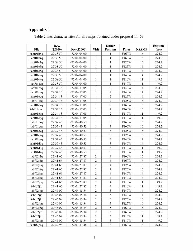
Appendix 1

Table 2 lists characteristics for all ramps obtained under proposal 11453.

File

R.A.

(J2000) Dec (J2000) Visit

Dither

Position Filter NSAMP

Exptime

(sec)

iabf01bxq 22:38.50 -72:04:04.00 1 1 F160W 16 274.2

iabf01bzq 22:38.50 -72:04:04.00 1 1 F160W 16 274.2

iabf01c1q 22:38.50 -72:04:04.00 1 1 F125W 16 274.2

iabf01c3q 22:38.50 -72:04:04.00 1 1 F125W 16 274.2

iabf01c5q 22:38.50 -72:04:04.00 1 1 F140W 14 224.2

iabf01c7q 22:38.50 -72:04:04.00 1 1 F140W 14 224.2

iabf01c9q 22:38.50 -72:04:04.00 1 1 F110W 11 149.2

iabf01caq 22:38.50 -72:04:04.00 1 1 F110W 11 149.2

iabf01ccq 22:34.13 -72:04:17.05 1 2 F140W 14 224.2

iabf01ceq 22:34.13 -72:04:17.05 1 2 F140W 14 224.2

iabf01cgq 22:34.13 -72:04:17.05 1 2 F125W 16 274.2

iabf01ciq 22:34.13 -72:04:17.05 1 2 F125W 16 274.2

iabf01ckq 22:34.13 -72:04:17.05 1 2 F160W 16 274.2

iabf01cmq 22:34.13 -72:04:17.05 1 2 F160W 16 274.2

iabf01coq 22:34.13 -72:04:17.05 1 2 F110W 11 149.2

iabf01cpq 22:34.13 -72:04:17.05 1 2 F110W 11 149.2

iabf01crq 22:37.43 -72:04:40.53 1 3 F160W 16 274.2

iabf01ctq 22:37.43 -72:04:40.53 1 3 F160W 16 274.2

iabf01cvq 22:37.43 -72:04:40.53 1 3 F125W 16 274.2

iabf01cxq 22:37.43 -72:04:40.53 1 3 F125W 16 274.2

iabf01czq 22:37.43 -72:04:40.53 1 3 F140W 14 224.2

iabf01d1q 22:37.43 -72:04:40.53 1 3 F140W 14 224.2

iabf01d3q 22:37.43 -72:04:40.53 1 3 F110W 11 149.2

iabf01d4q 22:37.43 -72:04:40.53 1 3 F110W 11 149.2

iabf02j2q 22:41.66 -72:04:27.87 2 4 F160W 16 274.2

iabf02j4q 22:41.66 -72:04:27.87 2 4 F160W 16 274.2

iabf02j6q 22:41.66 -72:04:27.87 2 4 F125W 16 274.2

iabf02j8q 22:41.66 -72:04:27.87 2 4 F125W 16 274.2

iabf02jaq 22:41.66 -72:04:27.87 2 4 F140W 14 224.2

iabf02jcq 22:41.66 -72:04:27.87 2 4 F140W 14 224.2

iabf02jeq 22:41.66 -72:04:27.87 2 4 F110W 11 149.2

iabf02jfq 22:41.66 -72:04:27.87 2 4 F110W 11 149.2

iabf02jhq 22:46.09 -72:04:15.34 2 5 F140W 14 224.2

iabf02jjq 22:46.09 -72:04:15.34 2 5 F140W 14 224.2

iabf02jlq 22:46.09 -72:04:15.34 2 5 F125W 16 274.2

iabf02jnq 22:46.09 -72:04:15.34 2 5 F125W 16 274.2

iabf02jpq 22:46.09 -72:04:15.34 2 5 F160W 16 274.2

iabf02jrq 22:46.09 -72:04:15.34 2 5 F160W 16 274.2

iabf02jtq 22:46.09 -72:04:15.34 2 5 F110W 11 149.2

iabf02juq 22:46.09 -72:04:15.34 2 5 F110W 11 149.2

iabf02jwq 22:42.93 -72:03:51.48 2 6 F160W 16 274.2

2

iabf02jyq 22:42.93 -72:03:51.48 2 6 F160W 16 274.2

iabf02k0q 22:42.93 -72:03:51.48 2 6 F125W 16 274.2

iabf02k2q 22:42.93 -72:03:51.48 2 6 F125W 16 274.2

iabf02k4q 22:42.93 -72:03:51.48 2 6 F140W 14 224.2

iabf02k6q 22:42.93 -72:03:51.48 2 6 F140W 14 224.2

iabf02k8q 22:42.93 -72:03:51.48 2 6 F110W 11 149.2

iabf02k9q 22:42.93 -72:03:51.48 2 6 F110W 11 149.2

iabf03hpq 22:39.73 -72:03:27.55 3 7 F160W 16 274.2

iabf03hrq 22:39.73 -72:03:27.55 3 7 F160W 16 274.2

iabf03htq 22:39.73 -72:03:27.55 3 7 F125W 16 274.2

iabf03hvq 22:39.73 -72:03:27.55 3 7 F125W 16 274.2

iabf03hxq 22:39.73 -72:03:27.55 3 7 F140W 14 224.2

iabf03i2q 22:39.73 -72:03:27.55 3 7 F110W 11 149.2

iabf03i4q 22:35.31 -72:03:40.16 3 8 F140W 14 224.2

iabf03i6q 22:35.31 -72:03:40.16 3 8 F140W 14 224.2

iabf03i8q 22:35.31 -72:03:40.16 3 8 F125W 16 274.2

iabf03iaq 22:35.31 -72:03:40.16 3 8 F125W 16 274.2

iabf03icq 22:35.31 -72:03:40.16 3 8 F160W 16 274.2

iabf03ieq 22:35.31 -72:03:40.16 3 8 F160W 16 274.2

iabf03igq 22:35.31 -72:03:40.16 3 8 F110W 11 149.2

iabf03ihq 22:35.31 -72:03:40.16 3 8 F110W 11 149.2

iabf03ijq 22:30.89 -72:03:52.77 3 9 F160W 16 274.2

iabf03ilq 22:30.89 -72:03:52.77 3 9 F160W 16 274.2

iabf03inq 22:30.89 -72:03:52.77 3 9 F125W 16 274.2

iabf03ipq 22:30.89 -72:03:52.77 3 9 F125W 16 274.2

iabf03irq 22:30.89 -72:03:52.77 3 9 F140W 14 224.2

iabf03itq 22:30.89 -72:03:52.77 3 9 F140W 14 224.2

iabf03ivq 22:30.89 -72:03:52.77 3 9 F110W 11 149.2

iabf03iwq 22:30.89 -72:03:52.77 3 9 F110W 11 149.2

Table 2: Data characteristics. The dither position column follows the numbering scheme

presented in Figure 1. All ramps were obtained using the STEP25 sample sequence.

3

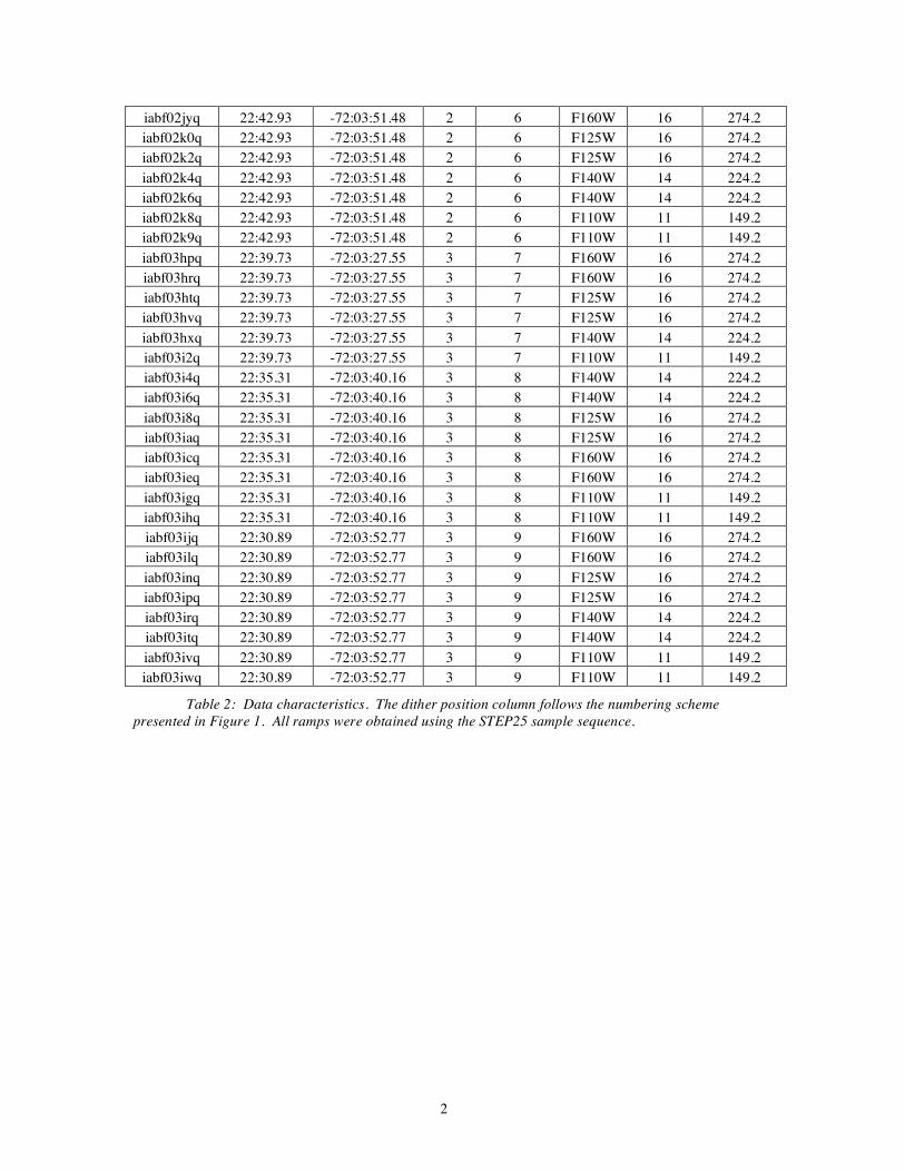
File Filename Purpose

BPIXTAB t291659ni_bpx.fits Bad pixel table

CCDTAB t2c16200i_ccd.fits** Detector calibration parameters

OSCNTAB q911321mi_osc.fits Detector overscan table

CRREJTAB t3j1659ki_crr.fits** Cosmic ray rejection parameters

DARKFILE t6119331i_drk.fits Dark current correction ramp

NLINFILE sbi18555i_lin.fits Non-linearity correction

coefficients

PFLTFILE sca20261i_pfl.fits Pixel-to-pixel flat field

GRAPHTAB t2605492m_tmg.fits HST graph table

COMPTAB t6i1714pm_tmc.fits HST components table

Table 3: Reference files used for all ramps collected in this proposal. Files listed in both of these tables

can be obtained from the HST archive. For more reliable photometry results, we edited the CCDTAB and

CRREJTAB files listed below. Detector gain values in the CCDTAB file were changed to be 2.4 e-

/sec/pixel for all four quadrants. In the CRREJTAB file, the values in the badinpdq column (rows 8-22)

were set to 316. This ensured that all pixels flagged as bad, bad zero read, hot, unstable, or saturated were

given a value of zero in the final image.

1

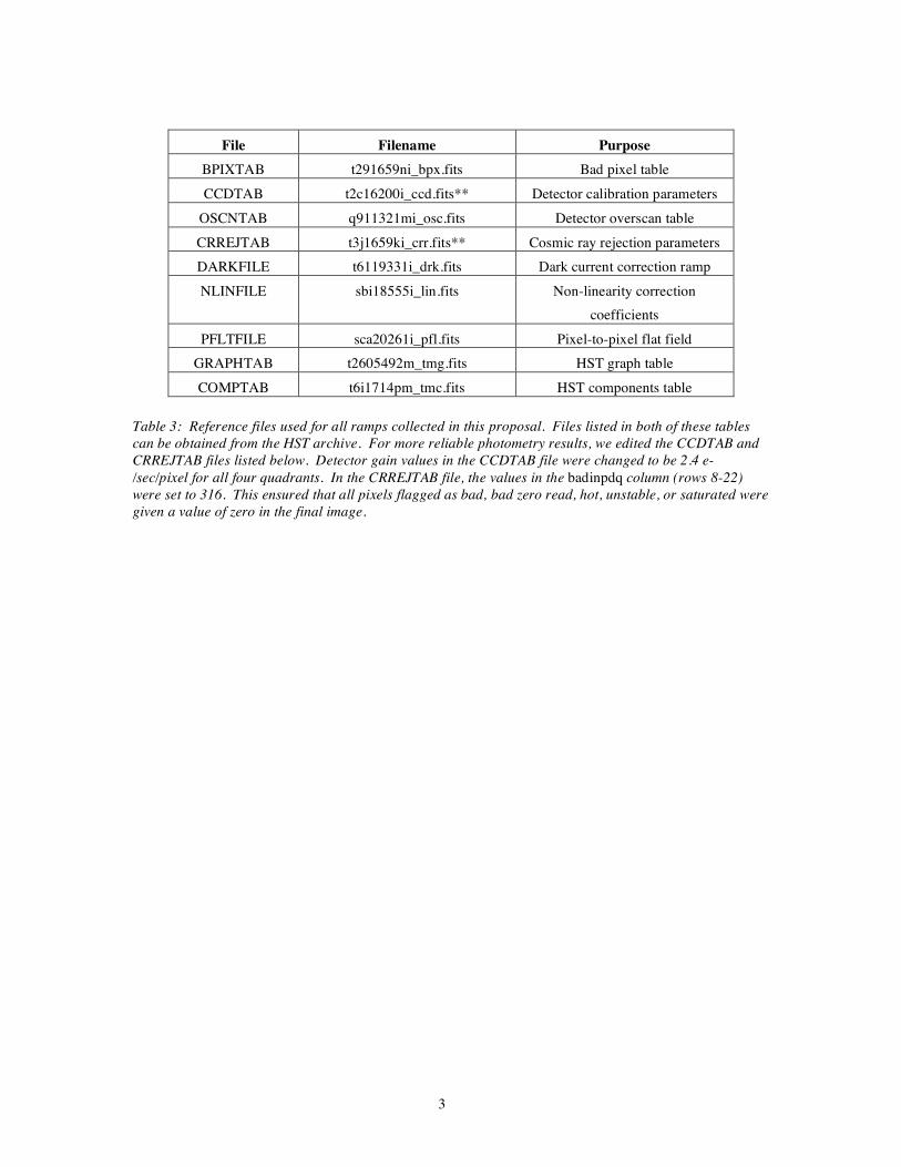
Appendix 2

Figures showing the positions of sources and the scatter in magnitude differences for

the F125W, F140W, and F160W filters.

Figure 5: Positions of the sources used in the analysis of the F125W data.

Figure 6: Scatter plots showing the variation of magnitude differences in four strips across the detector for

F125W.

2

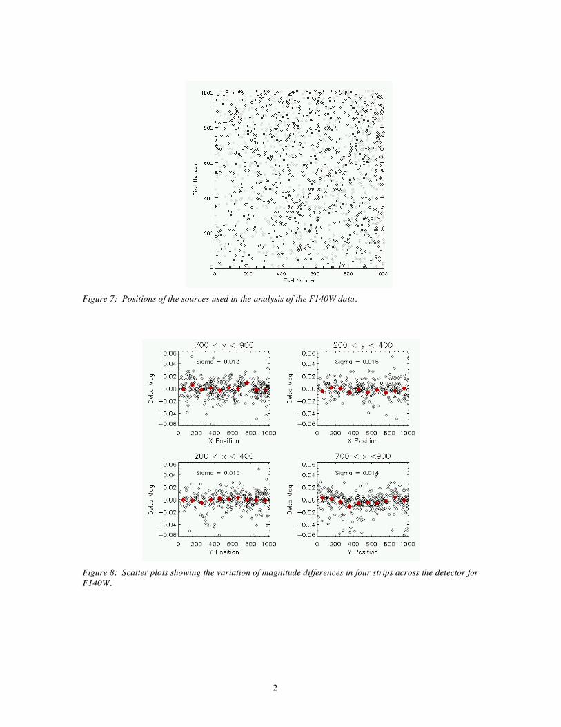
Figure 7: Positions of the sources used in the analysis of the F140W data.

Figure 8: Scatter plots showing the variation of magnitude differences in four strips across the detector for

F140W.

3

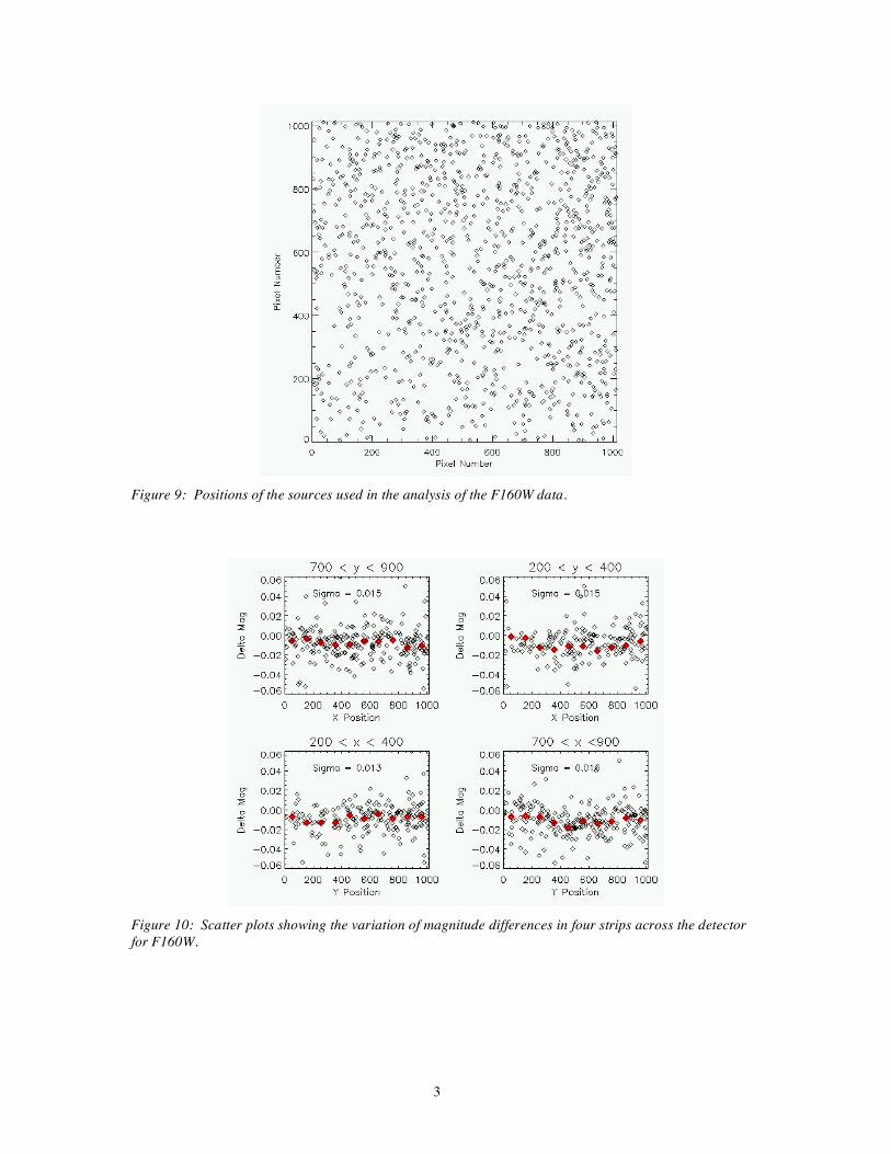
Figure 9: Positions of the sources used in the analysis of the F160W data.

Figure 10: Scatter plots showing the variation of magnitude differences in four strips across the detector

for F160W.