Wellformed Systems of Point Incidences for Resolving ...sitharam/overlap-j.pdf · Wellformed...

April 17, 2006 10:54 WSPC/Guidelines p

International Journal of Computational Geometry & Applicationsc© World Scientific Publishing Company

Wellformed Systems of Point Incidences

for Resolving Collections of Rigid Bodies

Meera Sitharam∗

CISE Dept. University of Florida

Gainesville, FL, 32611, US

[email protected]

Received (received date)Revised (revised date)

Communicated by (Name)

For tractability, many modern geometric constraint solvers recursively decompose aninput geometric constraint system into standard collections of smaller, generically rigidsubsystems or clusters. These are recursively solved and their solutions or realizationsare recombined to give the solution or realization of the input constraint system.

The recombination of a standard collection of solved clusters typically reduces topositioning and orienting the rigid realizations of the clusters with respect to each other,subject to incidence constraints representing primitive, shared objects between the clus-ters and other external constraints relating objects in different clusters.

Even for generically wellconstrained systems in 3D, and even when the shared objectsare restricted to be points, finding a system of incidence constraints that extends to awellconstrained system for recombining a cluster decomposition is a significant hurdlefaced by geometric constraint solvers. In general, we would like a wellformed systemof incidences that generically preserves the classification of the original, undecomposedsystem as a well, under or overconstrained system.

Here we motivate, formally state and give an efficient, greedy algorithm to find such awellformed system for a general constraint system, when the shared objects in the clusterdecomposition are restricted to be points. Our solution relies on isolating an interestingnew matroid structure underlying collections of rigid clusters with shared point objects.

Keywords: Decomposition and Recombination of Geometric Constraint Systems; Vari-ational Geometric Constraint Solving; Constraint graphs; Generic and CombinatorialRigidity; Matroids.

1. Introduction and Motivation

Geometric constraint systems are used as succinct, conceptual, editable representa-

tions of geometric composites in many applications including mechanical computer

aided design, robotics, molecular modeling and teaching geometry. For recent re-

views of the extensive literature on geometric constraint solving and basic defini-

tions, see expository papers in this volume and e.g, 2,11,10,15.

∗Work supported in part by NSF Grants EIA 02-18435, CCF 04-04116.

1


2 Meera Sitharam

For tractability of solving, many modern geometric constraint solvers use a com-

binatorial structure called a decomposition - recombination (DR) plan 2 to recur-

sively decompose an input geometric constraint system into collections of smaller,

generically rigid subsystems or clusters. These are recursively solved and their solu-

tions or realizations are recombined to give the solution or realization of the input

constraint system. The standard cluster decompositions (discussed in Section 2)

have many desirable properties that facilitate not only solving efficiency, but also

detecting rigidity, incorporating feature hierarchies, dealing with under and over-

constraints, solution navigation, 15.

The recombination of such a standard collection of solved clusters typically re-

duces to positioning and orienting the rigid bodies - i.e., the realizations of the

clusters - with respect to each other, subject to primarily incidence constraints rep-

resenting primitive, shared objects between the clusters and possibly other external

constraints relating objects in different clusters.

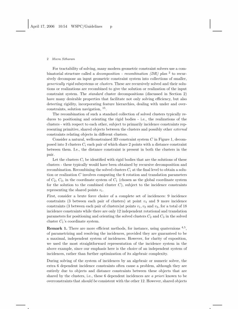
Consider a natural, wellconstrained 3D constraint system C in Figure 1, decom-

posed into 3 clusters Ci each pair of which share 2 points with a distance constraint

between them. I.e., the distance constraint is present in both the clusters in the

pair.

Let the clusters Ci be identified with rigid bodies that are the solutions of these

clusters - these typically would have been obtained by recursive decomposition and

recombination. Recombining the solved clusters Ci at the final level to obtain a solu-

tion or realization C involves computing the 6 rotation and translation parameters

of C2, C3, in the coordinate system of C1 (chosen as the global coordinate system

for the solution to the combined cluster C), subject to the incidence constraints

representing the shared points vi.

First, consider a brute force choice of a complete set of incidences: 9 incidence

constraints (3 between each pair of clusters) at point v4 and 9 more incidence

constraints (3 between each pair of clusters)at points v1, v2 and v3, for a total of 18

incidence constraints while there are only 12 independent rotational and translation

parameters for positioning and orienting the solved clusters C2 and C3 in the solved

cluster C1’s coordinate system.

Remark 1. There are more efficient methods, for instance, using quaternions 4,5,

of parametrizing and resolving the incidences, provided they are guaranteed to be

a maximal, independent system of incidences. However, for clarity of exposition,

we used the most straightforward representation of the incidence system in the

above example, since our emphasis here is the choice of an independent system of

incidences, rather than further optimization of its algebraic complexity.

During solving of the system of incidences by an algebraic or numeric solver, the

extra 6 dependent incidence constraints often cause a problem, although they are

entirely due to objects and distance constraints between these objects that are

shared by the clusters, i.e., these 6 dependent incidences are a priori known to be

overconstraints that should be consistent with the other 12. However, shared objects


Wellformed Systems of Point Incidences for Resolving Collections of Rigid Bodies 3

C1 C2

C3

v1v2

v3

v4

3

3

2:x,y

2:x,y 1:z

1

2

2

3

3

2

3

3 2

2

2

Fig. 1. Choosing wellconstrained sets of incidences is nontrivial: see text

and constraints are replicated and treated separately in the participating clusters Ci

when they are independently solved, typically by finite precision computations. As

a result, the 6 dependent incidence constraints typically turn out to be inconsistent

with the other 12. For example, the actual distance between the solved points v1

and v4 in C2 may not exactly equal the distance between the copies of the same

points in C3.

Remark 2. Some algebraic and numeric solvers incorporate methods for dealing

with such overconstrained systems. For example, numeric solvers based on gradient

descent may circumvent this problem since each iteration solves a linear system

and overdetermined systems are simply solved by finding the best least squares fit.

However, such numeric solvers do not usually return all solutions. A more serious

drawback that is common to this type of approach and other general approaches

that adjust for finite precision inaccuracies by using tolerance intervals, or algebraic

approaches that deal with overdetermined systems using rational univariate repre-

sentations etc. is the following: they do not discriminate between the above type

of introduced-incidence overconstraints that are caused entirely by treating shared

objects as incidences (and are hence a priori known to be consistent), and other


4 Meera Sitharam

inherent overconstraints that were present in the original system C that relates

the clusters Ci (such as the example in Figure 6), which could moreover include

other external constraints relating objects in different Ci (not present in either of

these examples). Such a discrimination is desirable for most applications which re-

quire careful detection of inherent, implicit overconstraints. Some classical algebraic

methods could potentially be used to isolate specifically these global introduced-

incidence dependences, however, we contend that (a) it would be necessary for any

such method to solve the essentially combinatorial problem which we pose and solve

in this manuscript, and furthermore (b) such a combinatorial solution is sufficient

in generic cases.

We would like to explicitly avoid these introduced-incidence overconstraints or de-

pendences, while retaining any inherent overconstraints. Towards this end, we could

first attempt to detect all local dependences. As a second attempt at the above ex-

ample, notice that only 6 incidence constraints at point v4 are independent (for

example, 3 of them between C1 and C2 and 3 of them between C2 and C3; the

other 3 each complete a cycle of incidences and are hence give a locally detectable

dependence). Discarding these 3 reduces the number of incidences to 15, but they

still clearly form a dependent system.

As a third attempt, notice that the shared distance constraint between each pair of

clusters permits a total of only 5 independent incidence constraints between each

pair of clusters. To account for this type of local dependence, choose 3 incidence

constraints each at points v1, v2, v3, totaling 9, and only 4 independent incidences

at point v4 (for example, 2 incidences say for the x and y coordinates between C1

and C2 and 2 between C2 and C3). This reduces the number of incidences to 13,

but they are still clearly dependent.

As a fourth attempt, avoiding both the above types of local dependences and taking

care to choose only 12 incidences still does not guarantee an independent system.

For example, as in the top right in Figure 1, choosing 3 incidence constraints each

at points v2 and v3, 1 incidence at v3, 2 incidences for the x and y coordinates

between C1 and C2 at v4, 2 incidences for the x and y coordinates between C3 and

C1 at v4 and 1 locally independent incidence for the z coordinate between C2 and

C3 gives a total of 12 incidences - but we show later that the last incidence above

is dependent on the 10 incidences between C1 and C2 (at v3 and v4) and between

C1 and C3 (at v2 and v4).

Thus, to obtain an independent set of incidences, global dependences - caused by

shared constraints between the clusters - have to be detected. Independent (and

maximal) choices of incidence systems for the example in Figure 1 are the following.

One possibility shown on the bottom right of Figure 1 is to choose 2 incidence

constraints at each of the points v1, v2, v3, and 6 independent incidences at point

v4 (for example, 3 of them between C1 and C2 and 3 of them between C2 and C3).

Another possibility is shown on the bottom left of Figure 1 and is a modification

of the top right picture: choose 3 incidence constraints each, at points v1 and v2, 2



incidence constraints at v3, 2 incidences between C1 and C2 at v4 and 2 incidences

between C2 and C3 at v4.

The above example was chosen as a small, manageable example for illustrating the

problem solved in this manuscript. However, some aspects of this example could

cause some confusions which the following remarks should clarify.

Remark 3. In the Figure 1 example, many decomposition-recombination based ge-

ometric constraint solvers, including our FRONTIER solver 6,14, would not solve C

by recombining the shown Ci; as a result the above problem of detecting introduced-

incidence (global) dependences would simply not arise, as we clarify below.

On the surface, the above example exposition would remain unaffected if 3

explicit distance constraints were to be added to C, pairwise between v1, v2 and v3,

to create a new system C′, where the Ci’s would be overconstrained. However, as a

result of these 3 additional distance constraints, none of the Ci is a maximal proper

subcluster of C. In particular, there is a 4th (tetrahedral) cluster C4 consisting of the

4 points vi. The cluster C4 would share 3 points with C1 and can hence be combined

in 3D into a cluster C14, which for the same reason can be combined with C2 into a

cluster C124 (which is in fact a maximal proper subcluster of C′), which can finally

be combined with C3 to give the cluster C′. DR-planners such as FRONTIER’s find

such so-called complete, maximal decompositions 12,7 for recombining each of the

clusters C14 and C124, which appear in the DR-plan for C. With the new DR-plan for

C′, the problem explained in the above example does not arise because recombining

2 clusters that share 3 (or more) points into a single cluster is a simple process that

only requires solving a linear system to find the coordinates of the second cluster’s

objects in the first cluster’s coordinate system. This further preserves any inherent

overconstraints (not present in this example), for instance, when some 2 of the

shared points do not have an explicit shared constraint between them.

Now we observe that even if the example C in Figure 1 remains unaltered with

no extra distance constraints, the cluster C4 would still be found by DR-planners

such as FRONTIER’s 2003 version 14. This version detects all known types of

hidden or implicit dependencies 7, and uses a so-called complete, maximal, module

decomposition of clusters. Such a DR-plan will effectively introduce the 3 distance

constraints pairwise between v1, v2 and v3, which are implied by the rigidity of

the clusters Ci, although these constraints were not present in the input constraint

system C. Hence the module decomposition will include the tetrahedral cluster C4,

and successively the clusters C14 and C124, exactly as in the previous paragraph.

This discussion raises the question whether the problem explained earlier, of de-

tecting introduced-incidence dependences, ever arises during cluster recombination.

Figure 2 shows a natural example of a cluster and its decomposition, where the prob-

lem of detecting introduced-incidence dependences during recombination is present

even when complete, maximal, module decompositions are employed. Hence the

problem presented in this manuscript will have to be faced by any decomposition-

recombination based geometric constraint solver, including FRONTIER.


6 Meera Sitharam

v9 v8

v7

v11v10

C1

3

3 3

323

2

3

3 3

32

3

v5

2

3

22

2:y,z2:x,y

2

32

3

2

C2

C3

C4v6

C5

C6

v1

v2

v3v4 3

2

3

3 3

32

3

1:z

3

Fig. 2. An example where the problem of choosing wellformed systems of incidences persists evenafter non-explicit constraints - that are implied by clusters - are added. Top right shows a badchoice of incidences; the bottom two are wellformed choices.

Problem Statement and Contribution

Our input is general 2D or 3D constraint systems C, with the usual variety of objects

and constraints given earlier, along with a standard cluster decomposition D into

maximal subclusters (defined formally in Section 2), with the restriction that the

clusters share only share point objects.

The problem is to replace the shared points by a set of incidences between the

clusters in D such that the resulting system for recombining C (which further in-

cludes other external constraints between the clusters in D) satisfies 3 requirements.

The first requirement is that this resulting system does not contain new introduced-

incidence dependences that were not originally present in the undecomposed system

C. While the above examples concern wellconstrained systems C, the problem of

choosing a wellformed set of incidence constraints (defined formally in Section 2)

applies to under and overconstrained systems C as well. Specifically, in the case of

a wellconstrained systems C, there should be no dependences in the chosen system

of incidences.

Note that any system of incidences underlying a cluster decomposition of C



C1 C2v1

v2

v3v4

c1c2

c3

v21

v22v42

v43

v31

v33

v12v11

c1

c2

v1

v2

v3

v4

z2

x

y

z

c1

c2

v1

v2v3

v4

z2

−z2v′2

x

y

z

Fig. 3. Another decomposition example (top left), seam graph (top right) and extraneous solutionto chosen system of incidences: see text

does not introduce any new inconsistencies regardless of whether it is wellformed or

not, since it simply replicates and then equates shared objects between the clusters.

Hence the solution set of the resulting recombination system contains the solution

set of the original system C. In particular, the complete set of incidences (assuming

infinite precision computation is used to compute the cluster realizations) gives

exactly the solution set of the original system C.

On the other hand, extraneous solutions are entirely acceptable (and unavoidable)

for a wellformed (usually incomplete) system of incidences recombining C from a

cluster decomposition, i.e., solutions that are not solutions of the original system

C. See the simple example Figure 3, where a 3D constraint system C is decom-

posed into 2 clusters sharing 2 points and a distance constraint, with an additional

distance constraint d between unshared points v3 and v4 in the two clusters. Now

C can be recombined from C1 and C2 using a wellformed system consisting of the

distance constraint d and 5 incidence constraints, i.e., 3 incidences at point v1 and

2 for the x and y coordinates at point v2. However, we get one extraneous solution

assigning two different z values for the copies of the same point v2 in C1 and C2 re-

spectively. In Figure 3, the extaneous point is denoted v′2. It is entirely unavoidable

that even for wellconstrained systems C, one of these extraneous solutions turns out


8 Meera Sitharam

to be atypical, i.e., a non-zero-dimensional or flexible solution, for no matter which

independent system of incidences is used for recombining a wellconstrained system

C. However, whenever an appropriate, natural notion of genericity can be defined

for the class of constraint systems from which C is drawn, such atypical extraneous

solutions should be generically avoidable provided adequately many incidences are

chosen.

Thus a competing second requirement of our problem is that adequately many

incidences should be chosen so that they generically preserve the classification of a

generic C as overconstrained, wellconstrained or underconstrained. More precisely,

given a decomposition D for a constraint system C that is generically wellcon-

strained (resp. underconstrained or overconstrained), a system I(D) of adequately

many independent incidences should be chosen so that such that the following holds.

Let IC(D) be any resulting system for recombining C (i.e., including additional ex-

ternal constraints between child clusters of C). Except for a measure zero subset

of the generic neighborhood of C, for any other constraint system C′ in the neigh-

borhood of C, IC′(D) has the same generic classification as C. Here the system of

incidences should depend only on the decomposition D of the cluster C, and not

on the further structure or parameters of other constraints in C, for example the

other external constraints between child clusters.

Together, the two requirements assert a minimal system of incidences (based

only on the decomposition of C) that generically preserves the classification of any

generic C.

An alternative informal statement of the problem is the following. We view incidence

constraints as zero-distance constraints. We then require an efficient algorithm for

choosing a maximal set of incidences (again, based only on the decomposition of C)

such that the following holds. Take a generic perturbation of the chosen system of

incidences (into near-incidences using infinitesimal non-zero distances) while keep-

ing all other external constraints between the child clusters and internal constraints

within the child clusters exactly the same. The resulting system for recombination

should generically preserve the well, under or overconstrainedness of any generic

C (as formally described in the previous paragraph). It is easy to see that this

requirement would not be met by any dependent system of incidence constraints

e.g., in the first 4 cases of the example of Figure 1 - in general, there would be no

solution, even if C were wellconstrained. In fact, unlike the exact systems of inci-

dences in the previous paragraph, the solution set given by the perturbed system

of incidences is in general not a superset of the undecomposed C. All we require is

that the classification of C be generically preserved.

Finally, as a third requirement, we would like an efficient algorithm for choosing

such a system of incidences, given as input a standard cluster decomposition. Prefer-

ably, the algorithm should be greedy and would avoid combinatorial explosion of

choices as well as wrong choices and backtracking. For example, Figure 6 shows

a decomposition of an overconstrained system and Figure 9 is a wellformed set of



incidences for it that is found by the algorithm presented in Section 3. It preserves

the dependences of the original overconstrained system, but does not create any

new dependences.

Organization

Section 2 builds up the formal machinery and combinatorial properties of wellformed

systems of incidences. Section 3 (Corollary 2) gives a solution to the problem stated

here by taking advantage of an interesting new underlying matroid structure. Sec-

tion 4 offers conclusions and suggestions for further investigation.

2. Standard Decompositions, Wellformed sets of Incidences and

their properties

Recall that the problem is to give an efficient, combinatorial algorithm that takes

a standard cluster decomposition as input and outputs a wellformed system of

incidences. We carefully formalize these notions and their properties which form

the basis for the algorithm presented in Section 3.

Standard Decomposition

The first notion we formalize is a standard decomposition of a constraint system

into rigid clusters. This will be the input to the algorithm for choosing a wellformed

set of incidences.

Let C be a geometric constraint system with the usual variety of objects and

constraints given in Section 1, and D a collection of rigid clusters or subsystems

C1, C2, . . . of C.

Let VD and ED denote the set of objects and constraints of C that are shared

by more than 1 cluster in D. D additionally induces the following. A collection of

subsets ci of VD, where ci contains all the objects in VD that belong to cluster Ci;

and dually, for each v ∈ VD and e ∈ ED, the set Sv (resp. Se ) of ci’s that contain

v (resp. e).

The pair (C, D) is said to be a standard decomposition if the following hold.

(1) The clusters in D are rigid maximal proper cluster subsystems of C. I.e., there

is no proper subsystem of C that is rigid and properly contains any of them.

(2) The clusters in D form a complete covering set for C, i.e., their union includes

all the objects of C and no cluster is entirely contained in another cluster.

(3) The objects in VD represent point objects in the constraint system C, the

constraints in ED represent shared distance constraints in the constraint system

C.

(4) If C is a 3D constraint system, for any i, j, |ci ∩ cj | ≤ 2; alternately for any

triple of points u, v, w ∈ VD, |Su ∩ Sv ∩ Sw| ≤ 1 and for any pair of constraints

e, f ∈ ED |Se ∩ Sf | ≤ 1.


10 Meera Sitharam

If C is a 2D constraint system, then for any i, j, |ci ∩ cj | ≤ 1; alternately for

any pair of points u, v ∈ VD, |Su ∩ Sv| ≤ 1 and ED is empty.

Justification of Decomposition Requirements

First, the maximality in the first requirement as well as the second requirement are

satisfied by 3D geometric constraint solvers such as 14 which typically decompose

C into a complete collection of maximal proper subsystems that are generically

rigid clusters 7,12. Such decompositions are desirable for numerous purposes in-

cluding solution navigation, rigidity determination, dealing with over and under

constrainedness, optimizing algebraic complexity, incorporating feature hierarchies15 etc. This implies that any such decomposition satisfies one of two properties:

it contains exactly 2 clusters that intersect on more than 2 points (1 point in the

case of 2D) since their union would be rigid, or otherwise, no pair of clusters in the

decomposition intersects on more than 2 points (1 point in the case of 2D, hence

there are no shared constraints). In the former case, recombining the 2 clusters can

be done easily as a linear system solution as pointed out in the introduction under

Remark 2, and we do not need a set of incidences for doing so. Therefore, the fourth

requirement is a natural one.

Remark 4. The above explanation has a simple consequence in 2D: no pair of

clusters in the standard decomposition can share more than 1 point, i.e., there are

no shared constraints. Hence the only dependences are caused by local cycles of

incidences such as those removed by the second attempt in the Section 1 example.

However, we nevertheless include the 2D case in our exposition as it serves as a

consistency check of the concepts and algorithm developed here - i.e, in the 2D case

our algorithm will automatically reduce to simply detecting these local cycles of

incidences.

The third requirement restricts shared objects VD to be points - a possible

method of generalization to other types of shared objects is given in Section 4.

However, once the shared objects are restricted to be points, the requirement con-

cerning ED is entirely natural, since the only natural constraints between pairs of

points are incidence and distance constraints. Again to avoid confusion in expo-

sition, we avoid shared incidence constraints and in general, incidence constraints

within the clusters Ci. Since the Ci are already determined to be rigid clusters, this

can be easily achieved by simply identifying those pairs of points within each Ci.

Remark 5. On the surface, the definition of standard decomposition seems to

exclude module decompositions discussed in the latter part of Remark 2, and con-

sequently it seems to forbid clusters such as C4, in the unaltered example C in

Figure 1, which are formed by implied distance constraints pairwise between v1, v2

and v3. However, as discussed in the earlier part of Remark 2, note that a module

decomposition of C is a standard decomposition of some C′ of the same size, whose

constraint set is a superset of C’s. For the Figure 1 example, C′ explicitly contains

the distance constraints pairwise between v1, v2 and v3. Since our results apply to



all standard decompositions of all constraint sytems, they, in effect, apply to module

decompositions as well.

Note: With the above explanation, it should be clear that the 3D examples in

the various discussions in Section 1 effectively satisfy the requirements for being a

standard decomposition.

Adjusted Degrees of Freedom of a Standard Decomposition

Next we define a key quantity that will be used in defining wellformed set of inci-

dences for recombining a standard decomposition.

The Adjusted Degrees of Freedom (adof)(C, D, T ) of any subset T of clusters

in a standard decomposition D of a constraint system C is a natural expression

that automatically adjusts for explicit overconstraints and was first used in 7 and12, together with the notion of a canonical, complete, maximal decomposition of

C. For our purposes here, the adof is a straightforward combinatorial expression

for computing the generic number of degrees of freedom of a collection of maximal

clusters that overlap and have other external constraints between them. A formal

definition follows. First we define the usual degrees of freedom based on primitive

geometric objects and rigid bodies.

• If C is a 3D (resp. 2D) constraint system, for any point v ∈ VD, dof(v) = 3

(resp. 2); For any shared (distance) constraint e ∈ ED, dof(e) = 5 (as pointed

out in Remark 4, ED is empty in 2D). For any other cluster Ci ∈ D, dof(Ci) = 6

(resp. 3), unless Ci is a rotationally symmetric cluster, for example representing

a point in 2D or 3D, in which case dof(Ci) = 3 (resp. 2); or representing a pair

of points in 3D with a distance constraint between them, or a single fixed

length line segment in 3D. In this case, dof(Ci) = 5. For any subset of clusters

T ⊆ D, let XT define the set of nonshared, external constraints relating objects

in different clusters in T - these and the (nonshared) objects that they relate

could be of any of the usual variety of types given in Section 1. For any external

constraint x = (u, v), dof(x) is the number of degrees of freedom it removes from

its participating objects u and v.

• The expression for the Adjusted dof adof(C, D, T ) uses inclusion-exclusion:

∑

Q⊆T,|Q|≥1

(−1)|Q|−1dof (⋂

Ci∈Q

Ci) −∑

x∈XT

dof (x)

Remark 6. Notice that the nonshared external constraints and the (nonshared)

objects that they relate could be of any of the usual variety of types given in Section

1. The manner in which in this manuscript has no deeper technical significance

beyond ease of exposition. Other equivalent treatments are possible. Specifically,

the complete covering set requirement in the definition of a standard decomposition

can be tightened to cover not just all objects but also all constraints in C. This

would force each external constraint e = (u, v) between clusters to be treated as a


12 Meera Sitharam

separate “external constraint pseudo-cluster” whose dof is computed as: dof(v) +

dof(u) − dof(e). Such an external constraint pseudo-cluster would be permitted to

share one object each with 2 other clusters, and we permit such shared objects alone

to be of other types (than points). This treatment of external constraints reduces

to the method used in this manuscript. For example, while the adof expression

above would be modified to incorporate external constraint clusters directly in the

inclusion-exclusion formula, and the last term would disappear, it is clear that these

changes would not alter the value of the computed adof. Similarly, it will become

clear in Section 3 that the algorithm will always pick the incidences corresponding

to the 2 participating objects of such an external constraint pseudo-cluster, i.e., the

corresponding external constraint will always be included in the output system.

The above expression has exponentially many terms in |T |. Using the fourth require-

ment of a standard decomposition, we next show a much simpler Moebius inversion

formula 1 for adof.

Proposition 1. Let C be a 3D geometric constraint system and D be a standard

decomposition of C. Assume that The sets VD, ED, Sv, Se are defined as above. Let

T be any subset of D. Let T1 ⊆ T be the non-rotationally symmetric clusters,

T2 ⊆ T be the clusters with 1 rotational symmetry in 3D, T3 ⊆ T be the set of fully

rotationally symmetric clusters, with no rotational degrees of freedom, and XT be

the set of external constraints. Then adof(C, D, T ) =

6 ∗ |T1|+ 5 ∗ |T2|+ 3 ∗ |T3| −∑

x∈XT

dof (x)− 3∑

v∈VD

(|Sv ∩ T | − 1)+∑

e∈ED

(|Se ∩T | − 1)

In the 2D case, since ED and T2 are empty, this expression is

3 ∗ |T1| + 2 ∗ |T3| −∑

x∈XT

dof (x) − 2∑

v∈VD

(|Sv ∩ T | − 1)

Proof: The negative term involving external constraints in XT appears in both the

original and simplified expressions and is hence irrelevant. Consider the nonzero

summands of the original adjusted dof expression. For |Q| = 1, the summand is

6 ∗ |T1| + 5 ∗ |T2| + 3 ∗ |T3|, (respectively 3 ∗ |T1| + 2 ∗ |T3|, in 2D), giving the first

positive terms in the above expression.

Assuming that no pair of clusters in T have a shared constraint, i.e., if ED is

empty, (which is always the case in 2D) each point v ∈ VD contributes −3(|Sv ∩

T | − 1) (respectively −2(|Sv ∩ T | − 1) in 2D) to the summands corresponding to

|Q| ≥ 2, giving the relevant negative term in the above expression. This completes

the proof for 2D since no pair of clusters shares a constraint.

In 3D, when clusters in T share constraints, each such shared constraint e ∈ ED

contributes −5(|Se ∩ T | − 1) to the summands corresponding to |Q| ≥ 2. However,

if e = (u, v), the contribution of the vertices u and v have to be removed from

those summands, hence each such shared constraint e contributes −5(|Se ∩ T | −

1) + 3(|Se ∩ T | − 1) + 3(|Se ∩ T | − 1) = +(|Se ∩ T | − 1), which completes the proof

for 3D, since no pair of clusters has more than 1 shared constraint. 2



Observation 1.

(1) If a constraint system C is generically wellconstrained, then adof(C, D, D) = 6

in 3D and 3 in 2D. for all standard decompositions D.

(2) If the constraint system C generically has overconstrained subsystems, then the

adjusted dof depends on the particular standard decomposition. (Only in 2D

distance constraint systems, where Laman’s theorem holds, is the adjusted dof

independent of the standard decomposition).

(3) There are constraint systems that are not generically rigid (not generically well

or well-overconstrained), but whose adjusted dof for all standard decomposi-

tions is at most 6 in 3D, or 3 in 2D. (Again, 2D distance constraint systems are

well-behaved and this does not happen).

Remark 7. In the latter cases of the above observation, i.e, when the constraint

system C has generically overconstrained subsystems, the preferred, canonical de-

compositions 7,12 are the following types mentioned earlier. (1) A so-called complete,

maximal standard decomposition of C for which the adof gives the so-called general-

ized Laman count, which is at most 6 (3 in 2D) if the is constraint system is generi-

cally rigid. The converse is true for such decompositions provided all overconstraints

are known to be explicit: for such generically under-overconstrained systems, these

complete maximal decompositions guarantee an adjusted dof greater than 6 (3 in

2D). However, the converse is false even for such decompositions, if implicit depen-

dencies are present: known generically under-overconstrained counterexamples in

3D are systems that embed the so-called “bananas” or “hinge” structures and are

key to the famous 3D combinatorial rigidity characterization problem 3, 8,9. (2) A

complete maximal module decomposition of C which gives a so-called module dof

count 7 which is at most 6 (3 in 2D) if the constraint system is generically rigid,

(truth of converse is unknown, no known counterexamples). As mentioned in Re-

mark 5, these decompositions may not be standard for C, they are standard for

some (generically overconstrained) constraint system C′ whose constraint set is a

superset of C’s.

Note. For the remainder of this manuscript we will be concerned only about the last

2 summands of the adof expression in Proposition 1, which we call the removed dof

(rdof). Hence, the only information that will be needed in a standard decomposition

(C, D) is (VD, ED, {ci}), from which the sets Sv, Se can be derived for each v ∈

VD, e ∈ ED. Any other information in a constraint system C and the clusters in D

is henceforth irrelevant. Hence we will simply identify this tuple with a standard

decomposition which we will denote D and refer to the sets ci ⊆ VD as “clusters”

in D.

The following definition makes this precise.

Let D be a standard decomposition of a geometric constraint system. Assume

that the sets VD, ED, Sv, Se are defined as above. Let T be any subset of D. Then


14 Meera Sitharam

in 3D, rdof(D, T ) =

3∑

v∈VD

(|Sv ∩ T | − 1) −∑

e∈ED

(|Se ∩ T | − 1)

For the 2D case, ED is empty, and rdof(D, T ) =

2∑

v∈VD

(|Sv ∩ T | − 1)

Wellformed Set of Incidences

We are now ready to precisely define well-formed system of incidences.

An incidence constraint for recombination (short: incidence) of a standard clus-

ter decomposition D = (VD, ED, {ci}) of a 3D constraint system C is a triple

(v, {ci, cj}, l), where v ∈ VD represents the shared point at which the incidence is

asserted; ci, cj ∈ D, with i 6= j, represent the two clusters which are constrained to

be incident at v, and 1 ≤ l ≤ 3 denotes the particular coordinate (x, y or z) (of

the point v) which is equated by the incidence constraint. In case of 2D constraint

systems C, l ≤ 2.

Note: Section 1 describes how such a set of incidence constraints I(D) (if properly

chosen) yields an algebraic system that could be used for recombining the solved

clusters in D to obtain a realization of a (generic or nongeneric) constraint system

C. We denote this recombination system as IC(D). In fact, using the construction in

Section 1, it represents a family of algebraic systems, one for each solution choice for

each of the clusters in the decomposition D. Hence, when we refer to the realization

or solution set of IC(D), we include solutions taken over all of the solution choices

for the clusters in D.

Definition 1. A wellformed set of incidences I(D) for a standard decomposition

D of a constraint system satisfies the following.

(1) There is no local cycle of incidences. Formally, for any v, l, and k ≥ 3, if I(D)

contains

(v, {ci1 , ci2}, l), (v, {ci2 , ci3}, l), . . . , (v, {cik−1, cik

}, l)

then I(D) does not contain (v, {ci1 , cik}, l).

(2) For a subset of clusters T ⊆ D, let I(D, T ) denote those incidences (v, {ci, cj}, l)

in I(D) for which ci, cj ∈ T . For any T ⊆ D, |I(D, T )| ≤ rdof (D, T ).

(3) |I(D)| = rdof (D, D).

Remark 8. For the 2D case, notice that any system of incidences that avoids local

incidence cycles is automatically wellformed. I.e., in 2D the first requirement in

Definiton 1 of wellformed systems of incidences, automatically implies the second.

And any maximal system of incidences satisfying the first requirement automatically

satisfies the third requirement. As a check, not surprisingly, it will turn out that the



algorithm given in Section 3 reduces in the 2D case to picking a maximal system of

incidences that avoids local cycles.

3. Seam Graphs and Main Technical Results

A significant contribution of this section is a careful and appropriate definition of

a construct called the seam graph from which an underlying matroid emerges and

many of the results follow from basic matroid theory. A seam graph GD correspond-

ing to a standard decomposition D = (VD, ED, {ci}) of a constraint system is an

undirected graph:

GD := (V , E);V :=⋃

v∈VD

Vv; E := PE ∪ LE ;

PE :=⋃

v∈VD

PEv = {(u, w) : u, w ∈ Vv};LE :=⋃

e∈ED

Ee

The seam graph GD contains |Sv| copies (recall notation from Section 2) of each

point v ∈ VD. I.e, for each cluster ci in Sv (that shares v in the decomposition D),

we create a copy vi of the vertex v. These sets of vertices are denoted Vv. The edges

of GD are of two types. The first is the set PE of point seam edges that connect

every pair of vertices (u, w) in the set Vv (forming a complete graph) for each v.

The second is the set LE of line seam edges which consists of |Se| copies of every

edge e ∈ ED. I.e., for each edge (u, w) in ED, and each cluster ci in Se that shares

e in G, we create a copy (ui, wi) of the edge (u, w). These sets of edges are denoted

Ee. (These do not exist for seam graphs corresponding to 2D systems).

Figures 4, 5 show examples of seam graphs for the example standard decom-

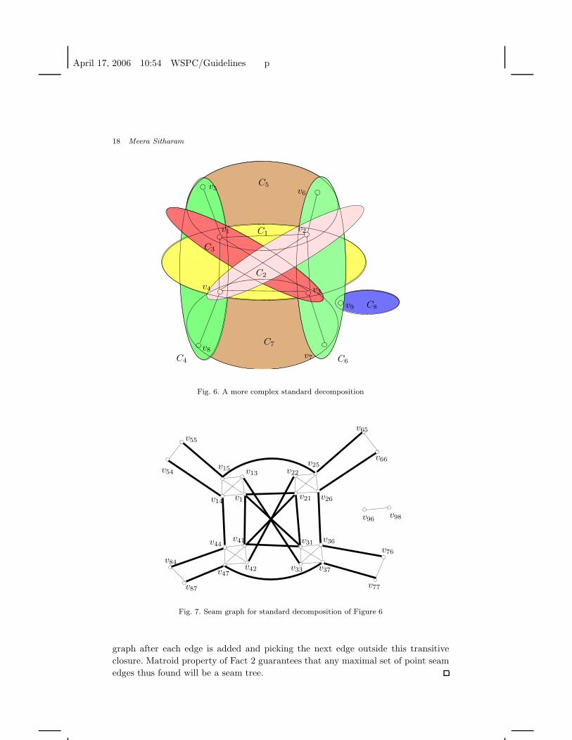
positions discussed in Section 1 and Figure 6 shows a more complex 3D standard

decomposition and Figure 7 shows the corresponding seam graph.

Note that any subset T ⊆ D of clusters of a standard decomposition D itself

satisfies relevant properties of a standard decomposition (covering potentially a

smaller subsystem of the original constraint system). Hence it also induces a seam

graph which we denote as GD,T .

A seam path is defined between or connecting a pair of vertices u, w in the same set

Vv of the seam graph GD. We denote a path as a sequence of consecutively incident

edges. The path assigns each of its edges a direction. A seam path between u and w,

u 6= w, is a simple path that is the concatenation of simple path segments h0, g1, . . . ,

h2m, g2m+1, . . . , h4m, where u and w are the first and last vertices of the first and

last edge on the path; and where the h2j ’s could be empty and consist only of point

seam edges (hence all edges in each h2j are necessarily are in the same set PEv for

some v). Each g2j+1 is a single edge in LE and has a unique partner edge g2l+1 such

that both edges belong to the same set Ee for some e = (x, y) ∈ ED. They appear

directed as (xi, yi) and (yk, xk) along the path and are associated with the clusters


16 Meera Sitharam

c1 c2

c3

v31 v32

v41 v42

v21

v23

v43

v13

v12

v31 v32

v41 v42

v43

v13

v12

g1 g3

g5

g7

h0

h2

h4

h6

h8

v31 v32

v41 v42

v21

v23

v43

v13

v12

v31 v32

v41 v42

v21

v23

v43

v13

v12

v31 v32

v41 v42

v21

v23

v43

v13

v12

Fig. 4. Top left shows seam graph for decomposition in Figure 1; seam path (top right), seamcycle (bottom left); and 2 seam trees corresponding to two wellconstrained incidences in bottomof Figure 1

ci and ck in Se. A seam cycle is a closed seam path, i.e., a seam path between u

and w, where u = w.

Figures 4 shows a seam path and a seam cycle for the standard decomposition in

Figure 1. We now define a number of special subgraphs of a seam graph. Seam

subgraphs are edge induced, spanning subgraphs i.e., they include all vertices, and

are line inclusive, i.e., they include all of the line seam edges in LE . Note: when the

context is clear, these subgraphs are simply identified with the set of their point

seam edges. A seam forest is a seam subgraph that does not contain any seam

cycles. A seam subgraph is seam connected if it contains a seam path between every

pair of vertices that belong to the same set Vv, for every v ∈ VD. A seam tree is a

seam forest that is seam connected. Seam trees are both minimal seam connected

subgraphs (removal of any point seam edge destroys seam connectedness) and the

maximal seam forests (addition of any point seam edge creates a seam cycle).

Figure 4 shows 2 seam trees for the seam graph of the standard decomposition

of Figure 1 that will be seen to correspond to the 2 wellconstrained choices of

incidences shown on bottom of Figure 1. Figure 8 shows a seam tree for the seam

graph of Figure 7, which corresponds to the standard decomposition of Figure 6.

This will be seen to correspond to a wellformed set of incidences of Figure 9. Figure

5 shows a seam graph corresponding to the example decomposition in Figure 2;

a seam tree which will be seen to correspond to a wellformed set of incidences in

Figure 2 as well as seam subgraphs containing seam cycles corresponding to the bad

choices of incidences in Figure 2. The next fact states that seam forests form the



c3

c4

c5

c6

v11

v21 v23

v13v12

v22v43 v33

v34v44

v54

v55v65

v62

v75

v76

v86v96

v81v91

v13

c2

c1

v11

v34v44

v54

v55v65

v62

v75

v76

v86v96

v81v91

v11

v21

v13v12

v22

v11

v21

v22

h0

g1

g3

h2

h4v12

v33v21 v23

v13v12

v22v43 v33

v34v44

v54

v55v65

v62

v75

v76

v86v96

v81v91

v11

v21 v23

v13v12

v22v43

Fig. 5. Seam graph; seam cycles corresponding to the bad choice of incidences and seam treescorresponding to wellformed choices of incidences in Figure 2

independent sets of a matroid and several properties immediately follow from basic

matroid theory. We refer the reader to 13 for matroid basics. It is straightforward

to check, using the properties of a standard decomposition in Section 2 and the

definition of the seam graph above that the matroid axioms are satisfied.

Fact 2. For a seam graph GD associated with a standard decomposition D, let F be

the collection of its seam forests (as noted, we identify a seam forest with its point

seam edges). Then the set PE of its point seam edges forms a matroid MD with F

as the collection of independent sets. We refer to this as a seam forest matroid. It

follows that the seam trees are the bases or maximal independent sets and they all

have the same size, namely the rank of the matroid.

Next we state the classical consequence of having an underlying matroid.

Theorem 3. A seam tree in a seam graph can be found using a greedy algorithm.

Proof. The algorithm starts with an empty set of point seam edges and picks

one point seam edge per iteration ensuring that at each iteration, seam cycles are

avoided. This can be done by simply taking the seam path transitive closure of the


18 Meera Sitharam

C1

C2

C3

C4

C5

C6

C7

C8

v1 v2

v3v4

v5 v6

v7

v8

v9

Fig. 6. A more complex standard decomposition

v21

v22

v25

v26

v41

v42

v44

v47

v54

v55

v31

v33

v36

v37

v65

v66

v84

v87

v76

v77

v98v96

v11

v13

v14

v15

Fig. 7. Seam graph for standard decomposition of Figure 6

graph after each edge is added and picking the next edge outside this transitive

closure. Matroid property of Fact 2 guarantees that any maximal set of point seam

edges thus found will be a seam tree.



v21

v22

v25

v26

v41

v42

v44

v47

v54

v55

v31

v33

v36

v37

v65

v66

v84

v87

v76

v77

v98v96

v11

v13

v14

v15

Fig. 8. Seam tree for seam graph of Figure 7

Theorem 4. Consider a seam graph GD of a standard decomposition D =

(VD, ED, {ci}) of a 3D constraint graph G. Then r =∑

v∈VD

(|Sv|−1)−∑

e∈ED

(|Se|−1)

is the rank of the underlying seam forest matroid MD.

Proof. We will show that

(i) a seam forest of GD has at most r point seam edges and

(ii) any seam connected subgraph has at least r point seam edges.

Thus a seam tree, which is a seam connected seam forest has exactly r point seam

edges, giving the rank of the matroid, from Fact 2.

Proof of (i): Start with a maximal seam forest F and extend it to a seam subgraph

F ∗ that includes a tree of edges from each complete graph PEv of point seam edges

associated with a vertex v of VD. Clearly the number of point seam edges in F ∗

is exactly∑

v∈VD

(Sv − 1). We will now show that |F ∗ \ F | is at least∑

e∈ED

(Se − 1),

thereby showing (i).

We can construct a maximal set W of pairs of the line seam edges LE such that

in each pair, both edges belong in the same set Ee for some e ∈ ED; and if (e1, e2),

(e2, e3), . . . , (em−1, em) are in the set, then (ej , ek) is not in the set for any j ≤ k−2,

with 1 ≤ j, k ≤ m. From the structure of a seam graph, |W | =∑

e∈ED

(Se − 1).

Crucially, since F is a maximal seam forest, and using the property of standard

decompositions given in Section 2 (i.e, no pair of clusters in D share more than

1 edge), each pair of edges in W , is associated with a unique corresponding edge

e∗ in F ∗ \ F , and together they define a unique seam cycle (minimal seam circuit)

associated with F , in F ∗: specifically all the other edges in such a seam cycle belong


20 Meera Sitharam

to F and removal of the cycle while retaining edges in F requires removing e∗. So

|W | is at most the number of such edges e∗ ∈ F ∗ \ F .

Proof of (ii): We now show that |F ∗ \F | is at most |W | for a collection W described

above. Take F to be minimal seam connected, hence for each edge e∗ ∈ F ∗\F , there

is a unique seam path in F that connects the 2 end points of e∗. This path contains

a unique pair of edges from a collection W as described above. So the number of

such edges e∗ is at most |W |.

From this, we obtain a simple result about wellformed sets of incidences.

Corollary 1. There is a wellformed set of incidences for a standard decomposition

D = (VD, ED, {ci}) of a 3D constraint graph G, containing at least 2∑

v∈VD

(|Sv| − 1)

incidences.

Proof. Specifically, it is sufficient to show that there is a set of incidences that

satisfies the first 2 wellformed properties and has size at least 2∑

v∈VD

(|Sv|−1), since

the 3rd wellformed property does not restrict the size. We construct such a set

of incidences J (D) as follows. J (D) :=⋃

v∈VD

J1,v ∪ J2,v where Jl,v consists of

exactly (|Sv|−1) incidences (v, {ci, cj}, l) (recall notation from Section 2). Here the

clusters ci, cj ∈ Sv contribute vertex copies vi and vj of v, in the seam graph GD.

The (|Sv| − 1) incidences are chosen so that the edges (vi, vj) form a tree in the

complete graph of point seam edges Pv associated with v in the seam graph GD.

We now show that this set of incidences satisfies the first 2 wellformed properties

of Section 2. It is clear that it does not contain any local incidence cycles, since the

edges (vi, vj) form a tree. To show the second wellformed property, for any subset

T ⊆ D, let J (D, T ) be the set of incidences restricted to T . Again, since the edges

(vi, vj) form a tree, it follows that for any T , |J (D, T )| ≤ 2∑

v∈VD

(|Sv ∩ T | − 1).

However, rdof (D, T ) was shown in Proposition 2 to be = 3∑

v∈VD

(|Sv ∩ T | − 1) −∑

e∈ED

(|Se ∩ T | − 1) for standard decompositions D.

Now we use Theorem 4, which shows that the quantity r =∑

v∈VD

(|Sv ∩T |− 1)−∑

e∈ED

(|Se ∩ T | − 1) is positive, since it is the rank of the seam forest matroid of the

seam graph GD,T induced by the subset T of the standard decomposition D. From

the expressions in the previous paragraph it follows that |J (D, T )| ≤ rdof (D, T )−r,

hence the second wellformed property holds for the set of incidences J (D), thus

completing the proof.

However, the above constructed set of incidences does not satisfy the last wellformed

property, for which we need the next result, which effectively solves the problem

stated in the introduction.



C2

C7

C5

C8

C4 C6

2 2

33

3

32

3

32

2

32

22

2 2

C3

C1

Fig. 9. Wellformed set of incidences corresponding to seam tree of Figure 8

Corollary 2. Given a 3D constraint graph G and a standard decomposition D =

(VD, ED, {ci}), there is a greedy algorithm running in time at most O((|VD ||D|)2)

for finding a wellformed set of incidences. Here |D| denotes the number of clusters

ci.

Proof. First we give the algorithm to construct a wellformed set of incidences

I(D).

Algorithm: Construct a seam tree F greedily as in the proof of Theorem 3. and

extend it as in the proof of Theorem 4 to F ∗ that includes a tree of edges from each

complete graph of point seam edges Pv associated with each v ∈ VD.

Now the first part of the construction of I(D) chooses incidences of the first two

coordinates and is similar to the construction of the set J (D) of incidences in the

proof of Corollary 1. For each v and each point seam edge (vi, vj) ∈ Pv ∩F ∗, put 2

incidence constraints (v, {ci, cj}, 1) and (v, {ci, cj}, 2) in I(D).

For the second part of the construction concerning incidences of the 3rd coordi-

nate, we turn to F . For each v, and each point seam edge (vi, vj) ∈ Pv ∩ F , put 1

incidence (v, {ci, cj}, 3) in I(D).

The running time of the entire procedure is at most quadratic in∑

v∈VD

(|Sv|) which

is at most O((|VD ||D|)2).

Figure 4 shows 2 seam trees from which the 2 wellconstrained sets of incidences

shown in Figure 1 are constructed using the above procedure. Similarly, Figure 9


22 Meera Sitharam

shows a wellformed set of incidences corresponding to the seam tree of Figure 8.

Why does I(D) satisfy the 3 wellformed properties? Since the construction only

uses only a tree of point seam edges (vi, vj) corresponding to each vertex v, and

for each of the 3 coordinates, we avoid local incidence cycles, satisfying the first

wellformed property.

Next we show the 3rd wellformed property. From the construction, the size |I(D)| =

2|F ∗|+ |F |. We have seen that |F ∗| =∑

v∈VD

(|Sv| − 1). And we know from Theorem

4 that |F | = r, the rank of the underlying seam forest matroid, which is∑

v∈VD

(|Sv|−

1) −∑

e∈ED

(|Se| − 1). Thus

|I(D)| = 3∑

v∈VD

(|Sv| − 1) −∑

e∈ED

(|Se| − 1)

which is exactly rdof(D, D), from Proposition 2.

The proof of the 2nd wellformed property simply uses the fact that for any subset

T of D, |I(D, T )| = 2|F ∗T | + |FT |, where F ∗

T and FT denote F ∗ and F restricted

(for each v ∈ VD) to those point seam edges (vi, vj) in Pv where the corresponding

clusters ci and cj both belong in Sv ∩ T . Now clearly |F ∗T | ≤

∑v∈VD

(|Sv ∩ T | − 1).

And since FT is a subgraph of the seam tree F , it has at most as many edges as

a seam tree for the seam graph GD,T induced by T . Hence |FT | ≤∑

v∈VD

(|Sv ∩ T | −

1) −∑

e∈ED

(|Se ∩ T | − 1). Thus

|I(D, T )| ≤ 3∑

v∈VD

(|Sv ∩ T | − 1) −∑

e∈ED

(|Se ∩ T | − 1) = rdof (D, T ),

where the latter equality is from Proposition 2.

4. Conclusions

By isolating an underlying matroid structure, we have given a simple algorithmic

solution to the informal problem stated in the introduction, satisfying the 3 given

requirements. To the best of our knowledge, neither this nor any similar prob-

lem has previously been studied in the literature although, for reasons detailed in

Section 1, we believe it would be a recurring problem for any general decomposition-

recombination based 3D constraint solver. The closest relative is Tay’s work 16,17

on body, panel, hinge and bar frameworks and structures, which have additional

restrictions that are crucial to his results. Hence those results do not extend to our

problem.

As pointed out earlier, we have considered in 5,4 the problem of optimizing the

algebraic complexity of the system of constraints for recombining a system C from

its cluster decomposition. However, in that work, we a priori assume the availability



of wellformed systems of incidences. Here, we show how to choose such systems. It is

our ongoing project to combine the two results, i.e., efficiently finding a wellformed

system that is also optimal in terms of algebraic complexity.

In addition, we believe that seam graph and seam forest matroid are independently

interesting and are likely to have further uses. We now present some directions in

which it would desirable to extend our results (or remove the restrictions under

which they apply) and provide concrete suggestions for doing so.

First, our results only have useful implications for generic constraint systems.

The drawback is that if the constraint repertoire is restricted, an appropriately

natural notion of genericity may not be definable. So for our algorithmic solution

to be meaningful in those contexts, it should contribute to an understanding of

non-generic situations.

Second, we have given a solution to the problem of finding wellformed systems

of incidences as defined in Section 2. To obtain an exact proof of implication to the

requirements in the problem statement of Section 1, we need to precisely formalize

the notion of genericity being used, which depends on the constraint repertoire, and

moreover the notion needs to be natural for the specific application.

Third, the shared objects between clusters in our decomposition are restricted

to be points, hence as pointed out in Section 2 the only natural shared constraints

are distance constraints between these points, (recall that shared constraints cause

the dependencies that our algorithm removes). In general, however, clusters could

share other objects such as lines, planes etc. causing a variety of shared constraint

possibilities.

The seam graph and seam forest matroid introduced here would be useful in ad-

dressing the first 2 issues mentioned above, as follows.

As mentioned earlier, the complete system of incidences for a cluster decompo-

sition of a constraint system C (assuming infinite precision computations), while

it contains dependencies, yields a recombination system that is equivalent to the

original system C and hence generically preserves the classification of C as well-

constrained, underconstrained or overconstrained. First note that if just enough

incidences are removed so that all local cycles eliminated - i.e., seam cycles that

consist only of point seam edges are eliminated, then the resulting recombination

system is still equivalent to the original system C. Such a system of incidences cor-

responds to a forest of trees of point seam edges, one maximal tree of point seam

edges corresponding to each shared vertex in the input decomposition of C. This

system which is refered to as F ∗ in the proof of Theorem 4, contains seam cycles

and we know the exact structure of further incidences that have to be removed to

obtain a seam tree F - i.e., the set F ∗ \ F . The removal of each of these incidences

creates a bifurcation of the original solution variety defined by the complete set of

incidences, i.e., the variety corresponding to C (potential extraneous solution vari-

eties are created by the bifurcations). It immediately follows that we can index the

extraneous solutions by subsets of removed incidences. Since the number of removed


24 Meera Sitharam

incidences is obtained directly from the rank of the underlying seam forest matroid,

we immediately have a nontrivial upperbound on the number of extraneous solution

varieties.

In fact, the seam tree F gives a simple algorithm to completely describe these

extraneous varieties: as mentioned in the proof of Theorem 4, each of these removed

incidences is associated with a unique seam cycle in the final seam tree F . Given a

seam cycle, it is associated with a unique pair of line seam edges (which corresponds

to a shared constraint between a specific pair of clusters in the decomposition of

C). These pairs form the set W in the proof of Theorem 4 and we know that for

any shared constraint e, the number of such line seam edge pairs is less than the

number of clusters sharing e, i.e., at most |Se| − 1. Thus each removed incidence

is associated with a unique (cluster) copy of a shared constraint in the input de-

composition. Hence a description of the extraneous variety indexed by a particular

subset of k removed incidences can be obtained directly from the original variety

corresponding to C and these k shared constraint copies. The efficiency of obtaining

these descriptions as well as the complexity of the descriptions (i.e., the “size” of

the polynomials in the description) can be reduced by choosing “short” seam trees

where all removed incidences would correspond to short cycles.

A key observation is that in the above discussion we have not used any genericity

properties of the original constraint system C or of the extraneous varieties, which

clearly indicates the usefulness of the seam graph in addressing the first issue above.

To address the second issue above, for wellformed systems of incidences obtained

from seam trees, observe that the structure and description of of extraneous varieties

discussed above gives us a simple method to eliminate those extraneous varieties

that are nongeneric over the reals (i.e., those that do not preserve the original classi-

fication of the constraint system C), by a real perturbation of C that infinitesimally

changes only the shared constraints in the given decomposition of C. It can be shown

that the original classification of a generic C as wellconstrained, underconstrained

or overconstrained would be preserved by all but a measure zero set of such pertur-

bations. This defines the precise notion of genericity under which we can formally

solve the first problem informally stated in Section 1. I.e., for generic C under this

definition, seam trees provide both minimal systems of incidences that still gener-

ically preserve the classification of C. Using a similar definition and argument, we

can use seam trees to formally state and solve the alternative problem statement

given in Section 1: seam trees provide maximal systems of incidences such that a

generic perturbation of these incidences still generically preserves the classification

of C. An interesting question remains: can similar implications be drawn for other

wellformed systems of incidences that satisfy the formal definition of Section 2, but

which are not obtained directly from seam trees, using the method described in

Corollary 2 (it is not hard to see that many such wellformed systems exist)?

To address the third issue above, one approach is to investigate if the seam graph

representation can be extended to include other types of shared objects and con-



straints and if the resulting introduced-incidence dependencies can be character-

ized via matroids or other combinatorial constructs. In fact, a systematic program

of investigation would be needed, starting with restricted classes of shared objects

and constraints and gradually enlarging or combining these classes. Our current

manuscript - which deals with shared point objects alone - can be viewed as the

first step in such a program of investigation.

Acknowledgement

We thank Yong Zhou for his gracious help in manuscript preparation.

References

1. M. Aigner. Combinatorial Theory. Springer, Classics in Mathematics Series, 1997.2. C. M. Hoffmann and A. Lomonosov and M. Sitharam. Decomposition of geometric

constraints systems, part i: performance measures. Journal of Symbolic Computation,31(4), 2001.

3. Jack E. Graver and Brigitte Servatius and Herman Servatius. Combinatorial Rigidity.Graduate Studies in Math., AMS, 1993.

4. M Sitharam and J Peters and Y Zhou. Solving minimal, wellconstrained, 3d geometricconstraint systems: combinatorial optimization of algebraic complexity. Automateddeduction in Geometry (ADG) 2004, available upon request, 2004.

5. Jorg Peters and JianHua Fan and Meera Sitharam and Yong Zhou. Elimination ingenerically rigid 3d geometric constraint systems. In Proceedings of Algebraic Geome-try and Geometric Modeling, Nice, 27-29 September 2004, pages 1–16. Springer Verlag,2005.

6. J. J. Oung and M. Sitharam and B. Moro and A. Arbree. Frontier: fully enablinggeometric constraints for feature based design and assembly. In abstract in Proceedingsof the ACM Solid Modeling conference, 2001.

7. M Sitharam and Y Zhou. A tractable, approximate, combinatorial 3d rigidity charac-terization. Fifth Automated Deduction in Geometry (ADG), 2004.

8. Henry Crapo. Structural rigidity. Structural Topology, 1:26–45, 1979.9. Henry Crapo. The tetrahedral-octahedral truss. Structural Topology, 7:52–61, 1982.

10. I. Fudos. Geometric Constraint Solving. PhD thesis, Purdue University, Dept of Com-puter Science, 1995.

11. G. Kramer. Solving Geometric Constraint Systems. MIT Press, 1992.12. Andrew Lomonosov. Graph and Combinatorial Analysis for Geometric Constraint

Graphs. Technical report, Ph.D thesis, Univ. of Florida, Gainesville, Dept. of Com-puter a nd Information Science, Gainesville, FL, 32611-6120, USA, 2004.

13. J.G. Oxley. Matroid Theory. Oxford University Press, 1992.14. M. Sitharam. Frontier, opensource gnu geometric constraint solver: Version 1 (2001)

for general 2d systems; version 2 (2002) for 2d and some 3d systems; version3 (2003) for general 2d and 3d systems. In http://www.cise.ufl.edu/∼sitharam,http://www.gnu.org, 2004.

15. M Sitharam. Graph based geometric constraint solving: problems, progress and direc-tions. In Volume on Computer Aided Design, D. Dutta R. Janardhan M. Smid ed.s,volume 67. AMS-DIMACS series, 2005.

16. T.S. Tay. Linking (n− 2)-dimensional panels in n-space: Part 2 (n− 2, 2)-frameworksand body and hinge structures. Graphs Combin, 5:245–273, 1989.


26 Meera Sitharam

17. T.S. Tay. Linking (n− 2)-dimensional panels in n-space: Part 1 (k − 1, k)-graphs and(k − 1, k)-frames. Graphs Combin, 7:289–304, 1991.

Wellformed Systems of Point Incidences for Resolving ...sitharam/overlap-j.pdf · Wellformed...

Documents

Transcript of Wellformed Systems of Point Incidences for Resolving ...sitharam/overlap-j.pdf · Wellformed...