
Well Log Interpretation
435
-
Upload
bilal-khan -
Category
Documents
-
view
648 -
download
15
description
well logging
Transcript of Well Log Interpretation

Developments in Petroleum Science, 1 5 A
fundamentals of well-log interpretation 1. the acquisition of logging data

FURTHER TITLES IN THIS SERIES
1 A.G. COLLINS
2 W.H.FERTL
3 A.P. SZILAS
4 C.E.B. CONYBEARE
GEOCHEMISTRY OF OILFIELD WATERS
ABNORMAL FORMATION PRESSURES
PRODUCTION AND TRANSPORT OF OIL AND GAS
GEOMORPHOLOGY O F OIL AND GAS FIELDS IN SANDSTONE BODIES 5 T.F. YEN and G.V. CHILINGARIAN (Editors)
OIL SHALE 6 D.W. PEACEMAN
7
8 L.P. DAKE
9 K.MAGARA
FUNDAMENTALS O F NUMERICAL RESERVOIR SIMULATION G.V. CHILINGARIAN and T.F. YEN (Editors)
BITUMENS, ASPHALTS AND TAR SANDS
FUNDAMENTALS O F RESERVOIR ENGINEERING
COMPACTION AND FLUID MIGRATION 10 M.T. SILVIA and E.A. ROBINSON
DECONVOLUTION O F GEOPHYSICAL TIME SERIES IN THE EXPLORATION FOR OIL AND NATURAL GAS
11 G.V. CHILINGARIAN and P. VORABUTR DRILLING AND DRILLING FLUIDS
1 2 T.D. VAN GOLF-RACHT FUNDAMENTALS O F FRACTURED RESERVOIR ENGINEERING
13 J. FAYERS (Editor) ENHANCED OIL RECOVERY
14 G. M6ZES (Editor) PARAFFIN PRODUCTS
Developments in Petroleum Science, 15A
well-log interpretation 1. the acquisition of logging data
0. SERRA Former Chef du Service Dhgraphies Differkes a la Direction Exploration
de la SNEA (P), Pau, France
and
Geological Interpretation Development Manager, Schlum berger Technical Services Inc., Singapore
(Translated from the French by Peter Westaway and Haydn A b b o t t )
ELSEVIER ELF AQUITAINE Amsterdam - Oxford - New York - Tokyo 1984 Pau
ELSEVIER SCIENCE PUBLISHERS B.V. Sara Burgerhartstraat 25 P.O. Box 21 1, 1000 AE Amsterdam, The Netherlands
Distributors for the United States and Canada:
ELSEVIER SCIENCE PUBLISHING COMPANY INC 52, Vanderbilt Avenue New York, NY 10017, U.S.A.
First edition 1984 Second impression 1985 Third impression 1988
Library of Congress Cataloging in Publication Data
Serra, Oberto. Fundamentals of well-log interpretation
(Developments in petroleum science; 15A- Translation of: Diagraphies differees. Bibliography: p. Includes index. Contents: v. 1. The aquisition of logging data. 1 . Oil well logging. I. Title. II. Series. TN87 1.35.S47 13 1984 622 ' . 18282 83-2057 1 ISBN 0-444-42132-7 (U.S.: V. 1)
ISBN 0-444-421 32-7 (Vol. 15A) ISBN 0-444-41 625-0 (Series)
@> Elsevier Science Publishers B.V., 1984
All rights reserved. No part of this publication may be reproduced, stored in a retrieval system or. transmitted in any form or by any means, electronic, mechanical, photocopying, recording or otherwise, without the prior written permission of the publisher, Elsevier Science Publishers B.V./ Physical Sciences & Engineering Division, P.O. Box 330, 1000 AH Amsterdam, The Netherlands.
Special regulations for readers in the USA -This publication has been registered with the Copyright Clearance Center Inc. (CCC), Salem, Massachusetts. Information can be obtained from the CCC about conditions under which photocopies of parts of this publication may be made in the USA. All other copyright questions, including photocopying outside of the USA, should be referred to the Dublisher.
No responsibility is assumed by the Publisher for any injury and/or damage to persons or property as a matter of products liability, negligence or otherwise, or from any use or operation of any meth- ods, products, instructions or ideas contained in the material herein.
Printed in The Netherlands
V
PREFACE
The relentless search for elusive hydrocarbon re- serves demands that geologists and reservoir en- gineers bring into play more and more expertise, inventiveness and ingenuity. To obtain new data from the subsurface requires the continual refinement of equipment and techniques.
This book describes! the various well-logging equipment at the disposal of geologists and reservoir engineers today. It follows two volumes on carbonates, also published by Elf Aquitaine.
One can never over-emphasize the importance to the geological analysis of basins, and sedimentology in general, of the information which drilling a bore- hole makes available to us. But this data would be incomplete, even useless, if not complemented by certain new techniques-well-logging in particular- which represent a tremendous source of information both about hydrocarbons and the fundamental geol- ogy of the rocks.
I t required considerable enthusiasm and a de- termination to succeed on the part of the author to bring the present work to its culmination, while at the same time performing the daily duties of Manager of the Log Analysis Section of the Exploration Dept. at Elf Aquitaine.
Such qualities, indeed, earned Oberto Serra the first Marcel Roubault award on March 21st, 1974, in just recognition of “work concerned with methods and techniques, or with ideas and concepts, which have led to important progress in the exploration for, and development of, natural energy resources, the discovery of new reservoirs, or the accomplishment of major works”. The judges recognized in particular an invaluable liaison between the spirit of the naturalist, constantly tempered by reality, and the rigorous
training of a physicist and informatician-bringing to the field of geological analysis all the facets of modern technology.
Since this award, 0. Serra has, by virtue of his talents as an instructor and author, acquired a very large audience both in professional circles and in the universities studying geological sciences.
This book is the result of a fruitful collaboration involving several companies. It testifies to the desire of Elf Aquitaine to further an active policy of re- search and training, disseminating knowledge of modern technical developments amongst its field per- sonnel.
It is hoped, that, in publishing this work, and continuing the series, we may contribute to a better understanding of geological sciences and their meth- ods, fundamental to our search for energy and mineral resources.
We also hope to strengthen the bonds between the “ thinkers” and the “doers”, those involved in re- search, and those on the operational side. Progress depends as much on the deliberations of the one, as on the techniques and skill of the other, and a close collaboration between the two is essential. Explora- tion is no longer an exclusive domain of guarded secrets; information gathered in the course of major projects must, wherever feasible, be made available to all interested, particularly those most likely to put it to good use.
Finally, let us hope that, with this publication, we might make a modest contribution to Marcel Roubault’s proud concept: “Geology at the service of Man”.
ALAIN PERRODON, Paris, March 1978

This Page Intentionally Left Blank
vii
FOREWORD TO THE FRENCH EDITION
The development of hydrocarbon reservoirs fol- lows complex natural laws dependent on a number of factors.
The geologist’s goal is to understand the processes of hydrwarbon accumulation. For, simply, the better these are understood, the better are the chances of discovering new hydrocarbon reserves.
The fields of geological study are several: sedi- mentology, structural geology, geochemistry, fluid geology, geophysics. Techniques are becoming con- tinually more sophisticated to keep pace with the demands of modern hydrocarbon exploration.
Well-logging plays a particularly important role in geophysics:
-well-logs provide an objective, continuous record of a number of properties of the rocks which have been drilled through;
-they are the link between geophysical measure- ments on the surface, and subsurface geology;
-they provide numerical data, introducing the possibility of fairly rigorous quantification in the description of sedimentological processes.
I t is no longer realistic to consider the geological description of a reservoir without incorporating log data, Its omission would effectively exclude most of the information potentially available from drill-holes, which itself represents a significant fraction of the total evidence on which the description can be based.
This book was conceived and written by a geolo- gist. I t is hoped it will provide geologists, (and, indeed, all engineers involved in hydrocarbon ex- ploration and reservoir development) with a good understanding of well-logging techniques, and an ap- preciation of the wealth of information available from log measurements, and their relevance in re- servoir description.
The present work is the first of a two-volume
series on well-logging. I t deals with the acquisition of log data (tool principles, logging techniques), and describes how the measurements are influenced by the many aspects of the geology of the rocks.
The second volume, currently under preparation, will cover in detail log interpretation and applica- tions.
ACKNOWLEDGEMENTS
I wish to express my thanks to my colleagues C. Gras, L. Sulpice and C . Augier of Elf Aquitaine, for their continual encouragement and constructive criticism of the first volume during its initial prepara- tion in French for publication; to G. Herve for his help in preparing the texts and figures for publica- tion; to P. Pain for his humorous illustrations; and to all anonymous draft-men and typists who contrib- uted to this book.
I also wish to express my gratitude to Schlum- berger for their permission to reproduce figures and texts from their various publications.
My thanks are also extended to Dresser-Atlas, SPE of AIME, and SPWLA from whose publications I have borrowed numerous figures.
Finally, I thank B. Vivet, Ph. Souhaite, J. Piger, J. Gartner and L. Dupal of Schlumberger Technical Services for their advice and criticism of the original French text; A. Perrodon for his constant support and encouragement; D. Bugnicourt for his advice on numerous points; H. Oertli for his invaluable assis- tance in editing and correcting the French text; and Elf Aquitaine for their permission to publish this book.
OBERTO SERRA. Paris, March 1978
... v l l l
FOREWORD TO THE ENGLISH EDITION
Following the suggestion of several people, I de- cided to translate my French book on Well Logging into English. At the same time I took the opportunity to improve and update the content by revising the original texts, correcting some errors which had eluded me, and adding sections on the most recent tech- niques. The critisms of reviewers of the original French text have been taken into account.
It considered that this translation could best be performed by my English colleagues within Schlum- berger. I wish to thank Peter Westaway and Haydn Abbott for undertaking this formidable task. Their contribution has been invaluable, both in translating
the French text and in bringing the present volume up to date.
1 should also like to mention the typists responsi- ble for preparing the final draft for editing.
Once again, I am indebted to H. Oertli for his help in the publication of this work, and to Elf-Aquitaine for their financial contribution without which this book could not have been published, and to Schlum- berger for their permission to reproduce some of their material.
OBERTO SERRA, Singapore, May 1982
ix
CONTENTS
Preface . . . . . . . . . . . . . . . . . . . . . . . . . . . . . . . . . . . . . Foreword to the French edition . . . . . . . . . . . . . . . . . . . . Foreword to the English edition . . . . . . . . . . . . . . . . . . .
Chapter 1 . 1.1. 1.2. 1.3. 1.3.1. 1.3.2. 1.3.3. 1.4. 1.4.1.
1.4.2.
1.4.3. 1.4.4. 1.4.5. 1.4.6. 1.5. 1.6.
Chapter 2 . 2.1. 2.1.1. 2.1.2.
2.2. 2.2.1. 2.2.2. 2.2.3. 2.2.4. 2.3. 2.3.1. 2.3.2. 2.3.3. 2.3.4. 2.3.5. 2.3.6. 2.4. 2.5. 2.6. 2.7.
Chapter 3 . 3.1. 3.2. 3.2.1. 3.2.2. 3.2.3. 3.2.4. 3.2.5. 3.2.6. 3.3. 3.3.1. 3.3.2. 3.3.3. 3.4. 3.4.1.
Review of basic concepts The definition of a " well-log'' . . . . . . . . . . . . The importance of well-logs . . . . . . . . . . . . . The definition of rock composition . . . . . . . . Matrix . . . . . . . . . . . . . . . . . . . . . . . . . . . . Shale, silt and clay . . . . . . . . . . . . . . . . . . . . Fluids . . . . . . . . . . . . . . . . . . . . . . . . . . . . . Rock texture and structure . . . . . . . . . . . . . . The relationship between porosity and resistiv- ity: the formation factor . . . . . . . . . . . . . . . . The relationship between saturation and resis- tivity: Archie's formula . . . . . . . . . . . . . . . . . The effect of shaliness on the resistivity The effect of shale distribution Permeability . . . . . . . . . . . . . . . . . . . . . . . . Thickness and internal structure of strata . . . . Conclusions . . . . . . . . . . . . . . . . . . . . . . . .
. . . . . . . .
. . . . . . . . . . . . . . . . . . . . . .
Logging techniques and measurements Classification of log measurements Natural phenomena . . . . . . . . . . . . . . . . . . . Physical properties measured by inducing re- sponses from the formation . . . . . . Problems specific to well-log measurements . . Borehole effects. invasion . . . . . . . . . . . . . . . The effect of tool geometry . . . . . . . . . . . . . . Logging speed . . . . . . . . . . . . . . . Hostile environments . . . . . . . . . . . . . . . . . . Loggng equipment-surface and downhole . . Logging truck and off Cable . . . . . . . . . . . . . . . . . . . . . . . . . . . . . The logging tool . . . . . . . . . . . . . .
Tool combinations . . Memorization . . . . . Log presentation . . . . . . . . . . . . . . . . . . . . .
Data transmission . . . . . . . . . . . . . . References . . . . . . . . . . . . . . . . . . . . . . . . .
Recording equipment . . . . . . . . . . . . . . . . . .
Repeatability and calibrations . . . . . . . . . . . .
The measurement of resistivity Introduction . . . . . . . . . . . . . . . . . . . . . . . . Non-focused long-spacing tools . . . . . . . . . . . Measuring principle . . . . . . . . . . . . . . . . . . . The current path . . . . . . . . . . . . . . . . . . . . . Measuring point . . . . . . . . . . . . . . . . . . . . . Radius of investigation . . . . . . . . . . . . . . . . . Environmental corrections . . . . . . . . . . . . . . The shape of the apparent resistivity curve . . . Focused long-spacing tools . . . . . . . . . . . . . .
The laterologs-LL . . . . . . . . . . . . . . . . . . . The spherically focused log-SFL . . . . . . . . .
Induction-IL . . . . . . . . . . . . . . . . . . . . . .
Non-focused microtools: the microlog (ML) . . Principle . . . . . . . . . . . . . . . . . . . . . . . . . . .
V
vii ...
Vl l l
1 1 2 2 2 5
11
12
14 15 15 18 23 24 24
29 29
29 30 31 33 36 38 38 39 39 43 44 45 45 46 48 48 50
51 51 51 53 53 54 54 55 57 51 64 61 71 11
3.4.2. 3.4.3. 3.5. 3.5.1. 3.5.2. 3.5.3. 3.5.4. 3.6. 3.6.1. 3.6.2. 3.1.
Chapter 4 . 4.1. 4.2. 4.2.1. 4.2.2. 4.2.3. 4.3. 4.4. 4.5. 4.5.1. 4.5.2. 4.5.3. 4.5.4. 4.5.5. 4.5.6. 4.5.7. 4.5.8. 4.6. 4.6.1. 4.6.2. 4.6.3. 4.6.4. 4.6.5.
4.1. 4.8.
Chapter 5 . 5.1. 5.2. 5.3. 5.4. 5.5. 5.6. 5.1. 5.8.
Chapter 6 .
6.1. 6.2. 6.2.1. 6.2.2. 6.2.3. 6.2.4. 6.2.5. 6.2.6. 6.3.
Environmental effects . . . . . . . . . . . . . . . . . Tool response . . . . . . . . . . . . . . . . . . . . . . . Focused microtools . . . . . . . . . . . . . . . . . . . The microlaterolog- MLC . . . . . . . . . . . . . . The microproximity log (PL) . . . . . . . . . . . . . The micro-SFL (MSFL) . . . . . . . . . . . . . . . . The high-resolution dipmeter (HDT) . . . . . . . Conclusions . . . . . . . . . . . . . . . . . . . . . . . . Geological factors which influence resistivity . Applications . . . . . . . . . . . . . . . . . . . . . . . . References . . . . . . . . . . . . . . . . . . . . . . . . .
The spontaneous potential -SP The origin of the electrokinetic potential The origin of the electrochemical potential . . . Membrane potential . . . . . . . . . . . . . . . . . . . Liquid junction or diffusion potential . . . . . . . The electrochemical potential. E, . . . . . . . . . . Ionic activity. concentration and resistivity . . . The static SP . . . . . . . . . . . . . . . . . . . . . . . . Amplitude and shape of SP peaks Hole diameter . . . . . . . . . . Depth of invasion . . . . . . .
. . . .
. . . . . . . . .
. . . . . . . . . . . . . . . . .
. . . . . . . . . . . . . . . . . Tight formations . . . . . . . . . . . . . . . . . . . . . Shale base-line shifts, and drift Irregular invasion profile . . . . . . . . . . . . . . . SP anomalies . . . . . . . . . . . . . . . . . . . . . . . . Geology and the SP . . . . . . . . . . . . . . . . . . . Composition of the rock . . . . . . . . . . . . . . . . Rock texture . . . . . . . . . . . . . . . . . . . . . . . . Temperature . . . Pressure . . . . . . . . . . . . . . . . . . . . . . . . . . . Depositional environment, sequential evolu- tion
References . . . . . . . . . . . . . . . . . . . . . . . . .
. . . . . . . . . . .
. . . . . . . . . . . . . .
. . . . . . . . . . . . . . . . . .
An introduction to nuclear logs Definition . . . . . . . . . . . . . . . . . . . . . . . . . . Recording capability . . . . . . . . . . . . . . . . . . Statistical variations . . . . . . . . . . . . . . . . . . . Dead-time . . . . . . . . . . . . . . . . . . . . . . . . . . Logging speed . . . . . . . . . . . . . . . . . . . . . . . Bed thickness . . . . . . . . . . . . . . . . . . . . . . .
References . . . . . . . . . . . . . . . . . . . . . . . . . Measuring point . . . . . . . . . . . . . . . . . . . . .
Measurement of the nature1 gamma radioactiv-
Definition natural radioactivity . . . . . . . . . . .
a-radiation . . . . . . . . . . . . . . . . . . . . . . . . .
itr
Basic concepts . . . . . . . . . . . . . . . . . . . . . . .
,&radiation. /3+ or f i - . . . . . . . . . . . . . . . . . . y-radiation . . . . . . . . . . . . . . . . . . . . . . . . . Radioactive decay . . . . . . . . . . . . . . . . . . . . Radioactive equilibrium . . . . . . . . . . . . . . . . The units of radioactivity . . . . . . . . . . . . . . . The origin of natural radioactivity in rocks . . .
12 72 12 12 13 73 73 14 74 15 16
77 19 19 80 80 80 81 82 82 82 82 83 84 84 85 85 86 86 88 88 88
88 88 88
89 89 89 90 91 91 93 93
95 95 95 96 96 96 97 98 99

X
6.4.
6.4.1. 6.4.2. 6.4.3. 6.4.4. 6.5. 6.5.1. 6.5.2. 6.5.3. 6.5.4. 6.6. 6.7. 6.8. 6.9. 6.9.1. 6.9.2. 6.9.3. 6.9.4. 6.10. 6.1 1 . 6.12.
Chapter 7 . 7.1. 7.2. 7.3. 7.4. 7.5. 7.6.
7.7. 7.8. 7.9. 7.9.1. 7.9.2. 7.9.3. 7.9.4. 7.9.5. 7.9.6. 7.9.7. 7.9.8. 7.9.9. 7.9.10. 7.9.11. 7.10. 7.10.1.
7.10.2. 7.10.3. 7.10.4. 7.10.5. 7.11.
Chapter 8 . 8.1. 8.2. 8.2.1. 8.2.2.
8.2.3. 8.2.4. 8.2.5. 8.2.6. 8.2.7. 8.2.8. 8.2.9.
Minerals and rocks containing radioactive ele- ments Potassium-bearing minerals and rocks . . . . . . Uranium-bearing minerals and rocks . . . . . . . Thorium-bearing minerals and rocks . . . . . . .
Measurement of gamma radiation . . . . . . . . . Geiger-Mueller counter . . . . . . . . . . . . . . . . Ionization chamber . . . . Scintillation counter . . . . Response of the tool . . . . . . . Measuring point . . . . . . . . . Radius of investigation . . . . . . . . . . . . . . . . .
Summary . . . . . . . . . . . . . . . . . . . . . . . . . .
Vertical definition . . . . . . . . . . . . . . . . . . . . Factors affecting the gamma-ray response . . . Statistical variations . . . . . . . . . . . . . . . . . . .
Bed thickness . . . Applications . . . . . . . . . . . . . . . . . . . . . . . .
References . . . . . . . . . . . . . . . . . . . . . . . . .
Natural gamma-ray spectrometry Principles . . . . . . . . . . . . . . . . . . . . . . . . . . Tool description . . . . . . . . . . . . . . . . . . . . .
Calibration . . . . . . . . . . . . . . . . . . . . . . . . .
Fundamental factors influencing the mea- surement . . . . . . . . . . . . . . . . . . . . . . . . . . . Computation of Th. U and K content . . . . . . Filtering . . . . . . . . . . . . . . . . . . . . . . . . . . . Applications . . . . . . . . . . . . . . . . . . . . . . . . Lithology determination . . . . . . . . Well-to-well variations . . . . . . . . . Detection of unconformities . . . . . . . . . . . . . Fracture and stylolite detection . . . . . . . . . . . Hydrocarbon potential . . . . . .
Sedimentology . . . . . . . . . . . . . . . . . . . . . . .
Radius of investigation . . . . . . . . . . . . . . . . .
Igneous rock recognition . . . . . . . . . . . . . . . .
Diagenesis . . . . . . . . . . Estimation of the uranium potential . . . . . . . . An approach to the cation exchange capacity .
Time constant (vertical smoothing). logging
The bore-hole . . . . . . . . . . . . . . . . . . . . . . . Tool position . . . . . . . . . . . . . . . . . . . . . . . . Casing . . . . . . . . . . . . . . . . . . . . . . . . . . . . Bed thickness . . . . . . . . . . . . . . . . . . . References . . . . . . . . . . . . . . . . . . . . . . . . .
Neutron logs
speed. dead time . . . . . . . . . . . . . . . . . . . . .
. . . . . . . . . . . . . . . ent hydrogen index .
Principles . . . . . . . . . . . . . . . . . . Spatial distribution of thermal neutrons and capture gamma rays . . . . . . . . . . . . . . . . . . .
Neutron sources .
Schlumberger neutron tools . . . . . . . . . . . . . Depth of investigation . . . Vertical resolution . . . . . . . . . . . . . . . . . . . . Measuring point . .
Calibration and log Its . . . . . . . . . . . .
_ . 8.2.10. Factors influencing the measurement . . . . . . .
99 99
101 105 106 106 106 106 107 107 108 108 109 109 109 109 109 110 111 111 111
113 114 114 116 119
119 120 120 121 121 126 126 126 128 129 130 131 132 132 132 132
132 132 133 133 133 133
135 135 135
138 138 139 139 140 141 142 142 142
8.2.11. Interpretation . . . . . . . . . . . . . . . . . . . . . . . 8.2.12. Environmental effects . . . . . . . . . . . . . . . . . 8.2.13.
8.2.14. Applications . . . . . . . . . . . . . . . . . . . . . . . . 8.3. References . . . . . . . . . . . . . . . . . . . . . . . . .
Geological factors affecting the hydrogen in- dex
Chapter 9 . 9.1.
9.1.1. 9.1.2. 9.1.3. 9.1.4. 9.2.
9.2.1. 9.2.2. 9.2.3. 9.2.4. 9.2.5. 9.2.6. 9.2.7. 9.3.
Induced gamma-ray spectrometry Early capture gamma-ray spectrometry- the chlorine log . . . . . . . . . . . . . . . . . . . . . . . . . Principle of the chlorine log . . . . . . . . . . . . . Measurement characteristics . . . . . . . . . . . . . The shale-compensated chlorine log (SCLL) . . Uses . . . . . . . . . . . . . . . . . . . . . . . . . . . . . . Modern induced gamma-ray techniques-in- elastic and capture spectrometry . . . . . . . . . . General . . . . . . . . . . . . . . . . . . . . . . . . . . . Fast neutron scattering . . . . . . . . . . . . . . . . . Thermal neutron capture . . . . . . . . . . . . . . . Reservoir analysis by spectroscopy . . . . . . . . Measured spectra . . . . . . . . . . . . . . . . . . . . . Measuring techniques-the window method . . The “weighed least-squares” (WLS) method . . References . . . . . . . . . . . . . . . . . . . . . . . . .
Chapter I0 . Thermal decay time measurements 10.1. 10.2. 10.2.1. 10.2.2. 10.2.3. 10.2.4. 10.3. 10.4. 10.5. 10.6. 10.7. 10.8. 10.9. 10.10, 10.11. 10.11.1. 10.1 1.2. 10.11.3. 10.11.4. 10.12. 10.12.1. 10.12.2. 10.12.3. 10.12.4.
10.13.
10.1 3.1. 10.13.2. 10.13.3. 10.13.4. 10.14. 10.14.1. 10.14.2. 10.15. 10.15.1. 10.15.2. 10.15.3. 10.15.4. 10.15.5. 10.16.
Background theory . . . . . . . . . . . . . . . . . . . . Tool principle . . . . . . . . . . . . . . . . . . . . . . . Neutron capture . . . . . . . . . . . . . . . . . . . . . Neutron diffusion . . . . . . . . . . . . . . . . . . . . Measuring the neutron population . . . . . . . . . Measurement of capture cross-section . . . . . . Neutron source . . . . . . . . . . . . . . . . . . . . . .
Spacing . . . . . . . . . . . . . . . . . . . . . . . . . . . Units . . . . . . . . . . . . . . . . . . . . . . . . . . . . . Calibration (see Appendix 5) . . . . . . . . . . . . . Measure points . . . . . . . . . . . . . . . . . . . . . . Vertical resolution . . . . . . . . . . . . . . . . . . . . Depth of investigation . . . . . . . . . . . . . . . . . Factors influencing the Z measurement . . The matrix ( X m a ) . . . . . . . . . . . . . . . . . . . .
Shales . . . . . . . . . . . . . . . . . . . . . . . . . . . . . Acidization . . . . . . . . . . . . . . . . . . . . . . . . . Environmental effects . . . . . . . . . . . . . . . . . Borehole signal and diffusion . . . . . . . . . . . . Tool eccentralization . . . . . Invasion . . . . . . . . . . . . . . . . . . . . . . . . . . . Time constant, logging speed. bed thickness and vertical resolution . . . . . . . . . . . . . . . . . Geological factors affecting the Z measure- ment Composition of the rock . . . . . Rock texture . . . . . . . . . . . . . . . . . . . . . . . . Temperature . . . . . . . . . . . . . . . . . . . . . . . .
Porosity and gas indication . . . . . . . . . . . . . .
Gas indication from the count- rates . Applications . . . . . . . . . . . . . . . . . . . . . . . . Response equations . . . . . . . . . . . . . . . . . . .
Formation fluid . . . . . . . . . . . . . . . . . . . . . .
Supplementary uses . . . . . . . . . . . . . . . . . . .
. . . . . . . . . . . . . . . . .
. . .
Porosity . . . . . . . . . . . . . . . . . . . . . . . . . . .
144 145
148 148 149
151 152 152 154 155
155 155 156 157 158 158 159 162 172
175 175 175 177 177 177 181 182 182 182 182 182 182 182 183 183 184 186 186 187 187 188 188
188
189 189 189 189 189 190 190 190 190 190 192 192 192 192 192

Chupier 11 .
11.1. 11.1.1. 11.1.2. 11.1.3. 11.2. 11.3.
11.4. 11.5. 11.6. 11.7. 11.8. 11.9. 11.10. 11.11.
11.11.1. 11.1 1.2. 11.1 1.3. 11.12. 11.13. 11.13.1.
11.13.2. 11.13.3. 1 1 . 13.4. 11.13.5. 11.14. 11.14.1. 11.14.2. 11.14.3. 11.14.4. 11.14.5. 11 .l4. 6.
11.15. 11.16.
Formation density measurements (the gamma-gamma log or density log) Principle . . . . . . . . . . . . . . . . Pair production . . . . . . . . . . . . . . . . . . . Cornpton scattering . . . . . . . . . . . . . . . . . . . Photo-electric effect . . . . . . . . . . . Absorption equation . . . . . . . . . . . . . . . . . . The relation between the electronic densit the bulk density . . . . . . . . . . . . . . . . . . Gamma-ray source . . . . . . . . . . . . . Detectors . . . . . . . . . . . . . . . . . . . Calibration units . . . . . . . . . . . . . . . . . The tools . . . . . . . . . . . . . . . . . . . . . . . . . .
Vertical resolution . . . . . . . . . . . . . . . . . . . .
men1 Shales . . . . . . . . . . . . . . . . . . . . . . . . . . . . . Water . . . . . . . . . . . . . . . . . . . . Hydrocarbon . . . . . . . . . . . . . . . . . . . . . . . . Interpretation . . . . . . . . . . . . Environmental effects . . . . . . . . . . . . .
thickness . . . . . . . . . . . . . . . . The borehole . . . . . . . . . . . . . . . . . . . . . . . . Mud-cake . . . . . . . . . . . . . . . . . . . . . . . . . . Casing . . . . . . . . . . . . . . . lnvasion . . . . . . . . . . . . . . . . . . . . . . . . . . . Geological factors . . . . . . . . . . . . . . . . . . . . Rock composition . . . . . . . . . . . . . . .
Sedimentary structure . . . . . . . . . Temperat . . . . . . . . . . . . . . . . . . . Pressure . . . . . . . . . . . . . . . . . . . Depositio ment-sequential evolu- tion Applications . . . . . . . . . . . . . . . . . References . . . . . . . . . . . . . . . . . . . . . . . . .
Rock texture . . . . . . . . . . . . . . . . . . . . . . . .
Chupter 12 . Measurement of the mean atomic number (litho-density tool)
12.1. Physical principle of the tool . . . . . . . . . . . . . 12.1.1. Photo-electric interaction . . . . . . . . . . . . . . . 12.1.2. Definition of the photoelectric absorption in-
dex 12.1.3. P, of a composite material . . . . . . . . . . . . . . . 12.2. The Schlumberger Litho- density tool (LDT) . 12.3. Principle of measurement . . . . . . . . . . . . . . .
12.5. Vertical resolution . . . . . . . . . . . . . . . . . . . . 12.6. Measuring point . . . . . . . . . . . . .
12.4. Radius of investigation . . . . . . . . . . . . . . . . .
12.7. 12.8.
12.9. 12.10. 12.10.1. 12.10.2. 12.10.3. 12.11.
Statistical variations . . . . . . . . . . . . . . . . . . Geological factors which affect the measure- ments Environmental effects on the measurements . Applications . . . . . . . . . . . . . . . . . . . . . . . Mineralogical composition of the formation . Fracture detection . . . . . . . . . . . . . . . . . . . Sedimentological studies . . . . . . . . . . . . . . . References . . . . . . . . . . . . . . . . . . . . . . . .
195 195 195 195 196
197 197 198 198 198 199 199 199
199 200 200 200 201 201
201 201 202 202 202 202 203 203 203 203 203
203 203 203
205 205
206 2G6 208 208 209 209 209 209
209 210 21 1 211 211 21 1 212
Chapter 13 . Acoustic log generalities-fundamentals 13.1. Acoustic signals . . . . . . . . . . . . . . . . . . . . . . 213 13.1.1. Period, T . . . . . . . . . . . . . . . . . . . . . . . . . . 213 13.1.2. Frequency, f . . . . . . . . . . . . . . . . . . . . . . . . 213 13.1.3. Wavelength, h . . . . . . . . . . . . . . . . . . . . . . . 213 13.2. Acoustic waves . . . . . . . . . . . . . . . . . . . . . . 213
13.2.1.
13.2.2. Transverse or shear waves (or S wave) . . . . . . 13.2.3. Surface waves . . . . . . . . . . . . . . . . . . . . . . . 13.3. Elastic properties of rocks . . . . . . . . . . . . . . . 13.4. Sound wave velocities . . . 13.5. Sound wave propagation, reflection and refrac-
tion 13.6. Acoustic impedance . . . . . . . . . . . . . . . . . . . 13.7. Reflection coefficient . . . . . . . . . . . . . . . . . . 13.8. Wave interference . . . . . . . . . . . . . . . . . . . . 13.9. References . . . . . . . . . . . . . . . . . . . . . . . . .
Compressional or longitudinal waves (or P wave)
Chapter 14 . Measurement of the speed of sound (Sonic
Log) Principle . . . . . . . . . . . . . . . . . . . . . . . . . . . 14.1.
14.2. Borehole compensated sonic . . . . . . . . . . . . . 14.3. Measure point . . . . . . . . . . . . . . . . . . . . . . . 14.4. Depth of investigation . . . . . . . . . . . . . . . . . 14.5. Vertical resolution . . . . . . . . . . . . . . . . . . . . 14.6. 14.7. 14.7.1. 14.7.2. 14.7.3. 14.7.4. 14.8. 14.9. 14.9.1. 14.9.2. 14.9.3. 14.9.4. 14.9.5. 14.9.6.
Units of measurement . . . . . . . . . . . . . . . . . Factors influencing the measurement . . . . . . . The matrix . . . . . . . . Porosity and fluids . . . . . . . . . . . . . . . . . . . .
Texture . . . . . . . . . . . . . . . . . . . . . Interpretation . . . . . . . . . . . . . . . . . . . . . . . Environmental and other effects . . . . . . . . . . Transit time stretching . . . . . . . . . . . . . . . . .
Kicks to smaller A t . . . . . . . . . . . . . . . . . . . The borehole . . . . . . . . . . . . . . . . . . . . . Invasion . . . . . . . . . . . . . . . . . . . . . . . .
Temperature and pressure . . . . . . . . . .
Cycle skipping . . . . . . . . . . . . . . . . . . . . . . .
Radial cracking effects . . . . . . . . . . . 14.10. Travel time integration . . . . . . . . . . . . . . . . . 14.11. Sonic log rescaling . . . . . . . . . . . . . . . . . . . . 14.12. Applications . . . . . . . . . . . . . . . . . . . . . . . . 14.1 3 . Determination of elasticity parameters using
14.14. References . . . . . . . . . . . . . . . . . . . . . . . . . logs . . . . . . . . . . . . . . . . . . . . . . . . . . . . . .
Chapter 15 . Measurement of sonic attenuation and ampli-
15.1. 15.1.1. Loss of energy through heat loss . . . . . . . . . . 15.1.2. Redistribution of energy . . . . . . . . . . . . . . . . 15.2. Causes of attenuation in the borehole . . . . . . . 15.2.1. Open-hole . . . . . . 15.2.2. Cased hole . . . . . 15.3. Measurement of attenuation 15.3.1. Cement Bond Log 15.3.2. Attenuation index . . . . . . . . . . . . . . . . . . . . 15.4. An expression for the law of attenuation in
15.5. Variable density log (VDL) . . . . . . . . . . . . . . 15.6. References . . . . . . .
tude Theoretical causes of attenuation . . . .
open hole . . . . . . . . . . . . . . . . . . . .
Chapter 16 . Measurement of the propagation time and at- tenuation rate of an electromagnetic wave (Electromagnetic Propagation Tool. EFT)
16.1. Generalities . . . . . . . . . . . . . . . . . . . . . . . . . 16.2. Basic concepts . . . . . . . . . . . . . . . . . . . . . . . 16.3. Theory of the measurement . . . . . . . . . . . . . . 16.4. Measurement technique . . . . . . . . . . . . . . . . 16.5. Depth of investigation . . . . . . . . . . . . . . . . . 16.6. Vertical resolution . . . . . . . . . . . . . . . . . . . . 16.7. Environmental factors influencing the response 16.7.1. Hole-size and shape . . . . . . . . . . . . . . . . . . .
214 214 215 215 216
216 217 217 217 218
219 223 224 224 224 225 225 225 226 226 221 228 230 230 231 231 231 232 233 233 234 235
236 236
239 239 239 240 240 242 242 242 244
246 247 250
251 251 251 252 254 254 255 255
xii
16.7.2. 16.7.3. 16.7.4. 16.8. 16.8.1. 16.8.2. 16.8.3. 16.9.
16.9.1. 16.9.2. 16.9.3. 16.9.4. 16.10. 16.11.
Chapter 17 17.1. 17.2. 17.3.
17.4.
Chapter 18 18.1. 18.1.1. 18.1.2. 18.2. 18.2.1. 18.2.2. 18.3.
Chapter 19 . 19.1. 19.2. 19.3. 19.4. 19.4.1. 19.4.2. 19.5. 19.5.1. 19.5.2. 9.5.3. 19.5.4.
19.5.5.
19.6. 19.6.1. 19.6.2. 19.6.3.
19.6.4.
19.6.5. 19.7. 19.7.1. 19.7.2. 19.7.3. 19.8. 19.8.1. 19.8.2. 19.8.3. 19.9.
Fluid . . . . . . . . . . . . . . . . . . . . . . . . . . . . . Mud-cake . . . . . . . . . . Temperature . . . . . . . . . . . . . . . . . . . . . . . .
Energy losses . . . . . . . . . . . . . . . . . . . . . . . . Interpretation in lossless formations . . . . . . . . Interpretation in lossy formations . . . . . . . . . Geological parameters affecting the measure- ment Mineralogical composition . . . . . . . . . . . . . . Texture . . . . . . . . . . . . . . . . . . . . . . . . . . . . Structure . . . . . . . . Fluids . . . . . . . . . . . . . . . . . . . . . . . . Applications . . . . . . . . . . . . . . . . . . . . . . . .
Borehole caliper measurements Principle . . . . . . . . . . . . . . . . . . . . . . . . . . Tools . . . . . . . . . . . . . . . . . . . . . . . . . . . . Geological factors influencing the hole diame- ter Applications . . . . . . . . . . . . . . . . . . . . . . .
Temperature measurements (temperature logs) Methods of temperature measurement . . . . . . Point measurements . . . . . . . . . . . . . . . . . . . Continuous temperature measurements . . . . . Applications . . . . . . . . . . . . . . . . . . . . . . . . Open hole . . . . . . . . . . . . . . . . . . . . . . . . . . Cased hole . . . . . . . . . . . . . . . . . . . . . . . . . References . . . . . . . . . . . . . . . . . . . . . . . . .
Dip measurements (dipmeter logs) Objective . . . . . . . . . . . . . . . . . . . . . . . . . . Principle . . . . . . . . . . . . . . . . . . . . . . . . . . . The measurement process . . . . . Dipmeter tools . . . . . . . . . . . . . . . . . . . . . . Discontinuous dipmeters . . Continuous dipmeters . . . . . . . . . . . . . . . . . Use of dipmeter resisti Description of raw log
Field magnetic tapes- . . . . . . . . Dip computation: Aut method . . . . . . . . . . . . . . . . . . . . . . . . . . . . Pattern recognition method of dip computa- tion Results presentation . . . . . . . . . . . . . . . . . . . Listing presentations Graphical presentatio Results given as punched cards or magnetic tapes . . . . . . . . . . . . . . . Horizontal or vertical proj deviation . . . . . . . . . . . . . . . . . . . . . . . . . . Special presentation of GEODIP results Treatment of results . . . . . . . . . . . . . . . . . . . The Cluster method . . . . . . . . . . . . . . . . . . . Determination of structural dip (Diptrend) . . . Dip-removal Applications Tectonic or st Sedimentary applications . . Stratigraphc applications . . . . . . . . . . . . . . . References
Dip computation: man . . . . . . . .
255 255 255 255 255 255 256
256 256 256 256 256 256 260
261 261
262 262
264 264 267 267 267 268 268
269 269 269 269 269 270 275 275 276 279
279
285 288 288 289
293
294 294 295 295 299 299 300 300 300 201 301
Chapter 20.1. 20.2. 20.2.1. 20.2.2. 20.2.3. 20.2.4. 20.3.
20 . Wireline sampling Rock sampling . . . . . . . . . . . . . . . . . . . . . . Fluid sampling and pressure measurements . . . Formation tester (FT) . . . . . . . . . . . . . . . . . Formation Interval Tester (FIT) . . . . . . . . . . Repeat Formation Tester (RFT) . . . . . . . . . . Fluid sampler applications . . . . . . . . . . . . . . References . . . . . . . . . . . . . . . . . . . . . . . . .
Chapter 21 . Other measurements 21.1. Borehole televiewer (BHTV) . . . . . . . . . . . . . 21.1 . 1. Principle . . . . . . . . . . . . . . . . . . . . . . . . . . . 21.1.2. Tool description . . . . . . . . . . . . . . . . . . . . . 21.1.3. Data recording and display . . . . . . . . . . . . . . 21.1.4. Parameters affecting the measurement . . . . . . 21.1.5. 21.1.6. 21.1.7. 21.2. 21.2.1. 21.2.2. 21.2.3. 21.2.4. 21.2.5. 21.3. 21.3.1. 21.3.2. 21.3.3. 21.3.4. 21.3.5.
Processing of the data . . . . . . . . . . . . . . . . . Interpretation . . . . . . . . . . . . . . . . . . Application . . . . . . . . . . . . . . . . . . . . . . . . . Vertical seismic profiling (VSP) . . . . . . . . . . . Principle . . . . . . . . . . . . . . . . . . . . . . . . . . .
. . . . . . . . . . Tool description . . Data recording . . . . . . . . . . . . . . . . . . . . . . Data processing . . . . . . . . . . . . . . . . . . . . . . Applications . . . . . . . . . . . . . . . . . . . . . . . . Nuclear magnetic log (NML) . . . . . . . . . . . . Introduction . . . . . . . . . . . . . . . . . . . . . . . . Principle . . . . . . . . . . . . . . . . . . . . . . . . . . .
Method of measurement . . . . . . . . . . . . . . . . Signal Processing . . . .
21.3.6. 21.3.7. Environmental factors . . . . . . . . . . . . . . . . 21.3.8. Interpretation-Application . . . . . . . . . . . . 21.4. References . . . . . . . . . . . . . . . . . . . . . . . .
Geological factor influencing the measurement
Chapter 22 . The place and role of logs in the search for petroleum . . . . . . . . . . . . . . . . . . . . . . . . . .
Appendix 1 . List of open hole logging tools and their symbol . . . . . . . . . . . . . . . . . . Specifica n hole logging tools . . . . Mathematics of manual dip computation . . . An example of a manual dipmeter calcula- tion Quick-look method todetermine the dip azimuth Quality control of log measurements . . . . . . General recommendations covering all oper- ations
Appendix 5A . Examples of logs with repeat section and calibrations for the most common Schlum- berger logs . . . . . . . . . . . . . . . . . .
. . . . . . . . . . . . . . . . . . Detailed calibration summaries . . . . . . . . . Induction logs DISF . . . . . . . . . . . . . . . . . Resistivity tools DLL-MSFL . . Nuclear tools FDC-CNL-GR . .
MLL- proximity . . . . .
ental and derived units. conversion tables . . . . . . . . . . . . . . . . . . .
Appendix 7.Quantities, their symbols and abbreviations . .
Appendix 2 . Appendix 3 .
Appendix 4 .
Appendix 5 .
Appendix 5B . CSU calibr
. . . . . . . . . . . . . . . . .
Index and Glossary . . . . . . . .
303 304 304 305 307 309
313 313 313 313 313 314 314 314 314 314 315 316 316 317 318 318 318 320 321 321 321 321 323 326
327
333 337 343
345
350 351
351
355 373 373 373 374 376 379 380
381 395 413
1
1. REVIEW OF BASIC CONCEPTS
1.1. THE DEFINITION OF A “WELL-LOG”
When we speak of a log in the oil industry we mean “a recording against depth of any of the char- acteristics of the rock formations traversed by a measuring apparatus in the well-bore.”
The logs we shall be discussing in this book, sometimes referred to as “wireline logs” or “well- logs”, are obtained by means of measuring equip- ment (logging tools) lowered on cable (wireline) into the well. Measurements are transmitted up the cable (which contains one or several conductors) to a surface laboratory or computer unit. The recording of this information on film or paper constitutes the well-log. Log data may also be recorded on magnetic tape. A large number of different logs may be run, each recording a different property of the rocks penetrated by the well.
Wireline logging is performed after an interruption (or the termination) of drilling activity, and is thus distinguished from “drilling-logs’’ (of such things as drilling-rate, mud-loss, torque, etc.) and “ mud-logs’’ (drilling mud salinity, pH, mud-weight, etc) obtained during drilling operations.
1.2. THE IMPORTANCE OF WELL-LOGS
Geology is the study of the rocks making up the Earth’s crust. The field of geology that is of most importance to the oil industry is sedimentology, for it is in certain sedimentary environments that hydro- carbons are formed, It entails a precise and detailed study of the composition, texture and structure of the rocks, the colour of the constituents, and identifica- tion of any traces of animal and plant organisms. This enables the geologist: (a) to identify the physi- cal, chemical and biological conditions prevalent at the time of deposition; and (b) to describe the trans- formations that the sedimentary series has undergone since deposition. He must also consider the organisa- tion of the different strata into series, and their possible deformation by faulting, folding, and so on.
The geologist depends on rock samples for this basic information. On the surface, these are cut from rock outcrops. Their point of origin is, obviously, precisely known, and in principle a sample of any desired size can be taken, or repeated.
Sampling from the subsurface is rather more prob- lematic. Rock samples are obtained as cores or cut- tings.
Cores obtained while drilling (using a core-barrel), by virtue of their size and continuous nature, permit a thorough geological analysis over a chosen interval. Unfortunately, for economical and technical reasons, this form of coring is not common practice, and is restricted to certain drilling conditions and types of formation.
“Sidewall-cores”, extracted with a core-gun, sam- ple-taker or core-cutter from the wall of the hole after drilling, present fewer practical difficulties. They are smaller samples, and, being taken at discrete depths, they do not provide continuous information. How- ever, they frequently replace drill-coring, and are invaluable in zones of lost-circulation.
Cuttings (the fragments of rock flushed to surface during drilling) are the principle source of subsurface sampling. Unfortunately, reconstruction of a litho- logical sequence in terms of thickness and composi- tion, from cuttings that have undergone mixing, leaching, and general contamination, during their transportation by the drilling-mud to the surf ace, cannot always be performed with confidence. Where mud circulation is lost, analysis of whole sections of formation is precluded by the total absence of cut- tings. In addition, the smallness of this kind of rock sample does not allow all the desired tests to be performed.
As a result of these limitations, it is quite possible that the subsurface geologist may find himself with insufficient good quality, representative samples, or with none at all. Consequently, he is unable to answer with any confidence the questions fundamental to oil exploration: (a) Has a potential reservoir structure been located? (b) If so, is it hydrocarbon-bearing? (c) Can we infer the presence of a nearby reservoir?
An alternative, and very effective, approach to this problem is to take in situ measurements, by running well-logs. In this way, parameters related to porosity, lithology, hydrocarbons, and other rock properties of interest to the geologist, can be obtained.
The first well-log, a measurement of electrical re- sistivity, devised by Marcel and Conrad Schlum- berger, was run in September 1927 in Pechelbronn (France). They called this, with great foresight, “elec- trical coring”. (The following text will demonstrate the significance of this prophetic reference to coring.) Since then scientific and technologd advances have led to the development of a vast range of highly sophisticated measuring techniques and equipment,
supported by powerful interpretation procedures. Well-log measurements have firmly established ap-
plications in the evaluation of the porosities and saturations of reservoir rocks, and for depth correla- tions.
More recently, however, there has been an increas- ing appreciation of the value of log data as a source of more general geological information. Geologists have realised, in fact, that well-logs can be to the subsurface rock what the eyes and geological instru- ments are to the surface outcrop. Through logging we measure a number of physical parameters related to both the geological and petrophysical properties of the strata that have been penetrated; properties which are conventionally studied in the laboratory from rock-samples. In addition, logs tell us about the fluids in the pores of the reservoir rocks.
The rather special kind of picture provided by logs is sometimes incomplete or distorted, but always permanent, continuous and objective. It is an objec- tive translation of a state of things that one cannot change the statement (on paper!) of a scientific fact.
Log data constitute, therefore, a “signature” of the rock; the physical characteristics they represent are the consequences of physical, chemical and biological (particularly geographical and climatic.. . ) condi- tions prevalent during deposition; and its evolution during the course of geological history.
Log interpretation should be aimed towards the same objectives as those of conventional laboratory core-analyses. Obviously, t h s is only feasible if there exist well-defined relationships between what is mea- sured by logs, and rock parameters of interest to the geologist and reservoir engineer.
The descriptions of the various logging techniques contained in this book will show that such relation- ships do indeed exist, and that we may assume: (a) a significant change in any geological characteristic will generally manifest itself through at least one physical parameter which can be detected by one or more logs; and (b) any change in log response indicates a change in at least one geological parameter.
1.3. DETERMINATION OF ROCK COMPOSI- TION
This is the geologist’s first task. Interpretation of the well-logs will reveal both the mineralogy and proportions of the solid constituents of the rock (i.e. grains, matrix * and cement), and the nature and
proportions (porosity, saturations) of the interstitial fluids.
Log analysts distinguish only two categories of solid component in a rock-“matrix” ** and “shale”. This classification is based on the sharply contrasting effects they have, not only on the logs themselves, but on the petrophysical properties of reservoir rocks (permeability, saturation, etc.). Shale is in certain cases treated in terms of two constituents, “clay” and “silt”. We will discuss this log-analyst terminology in more detail.
1.3.1. Matrix
For the log analyst, matrix encompasses all the solid constituents of the rock (grains, matrix *, ce- ment), excluding shale. A simple matrix lithology consists of single mineral (calcite or quartz, for exam- ple). A complex lithology contains a mixture of minerals: for instance, a cement of a different nature from the grains (such as a quartz sand with calcitic cement).
A clean formation is one containing no apprecia- bIe amount of clay or shale.
(Thus we may speak of a simple shaly sand lithol- ogy, or a clean complex lithology, and so on).
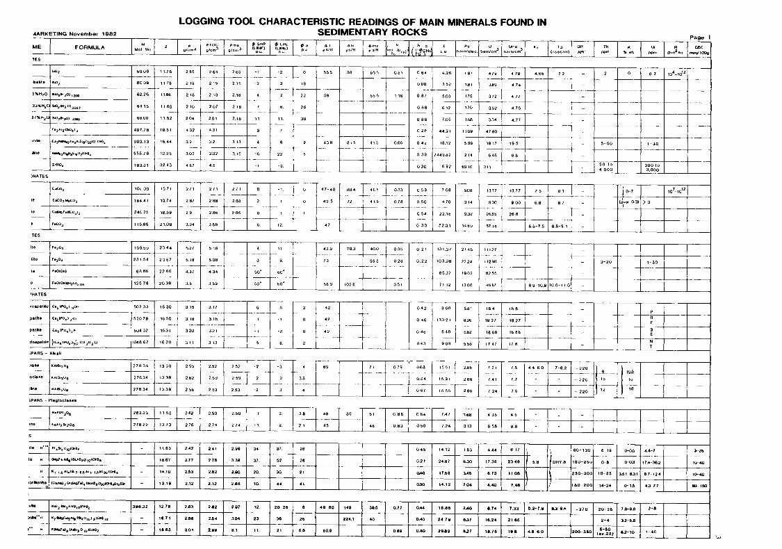
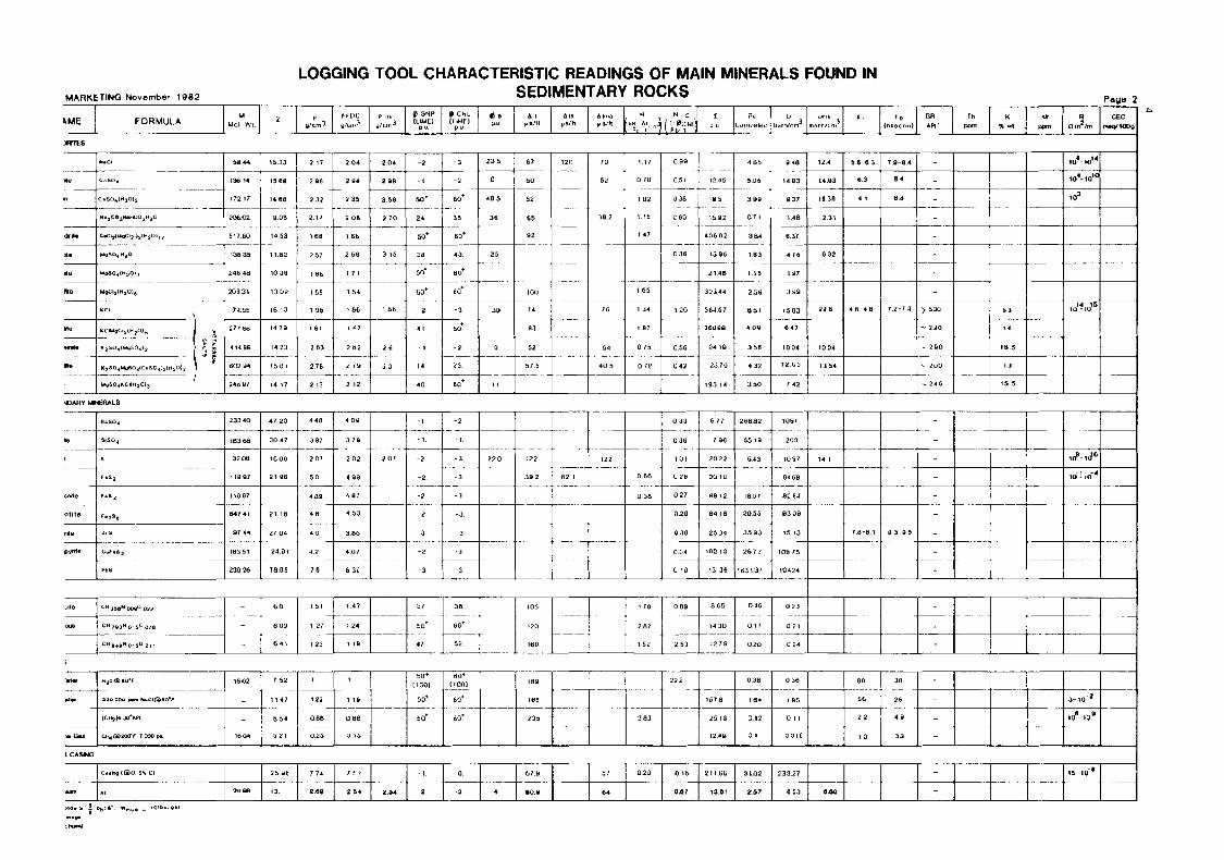
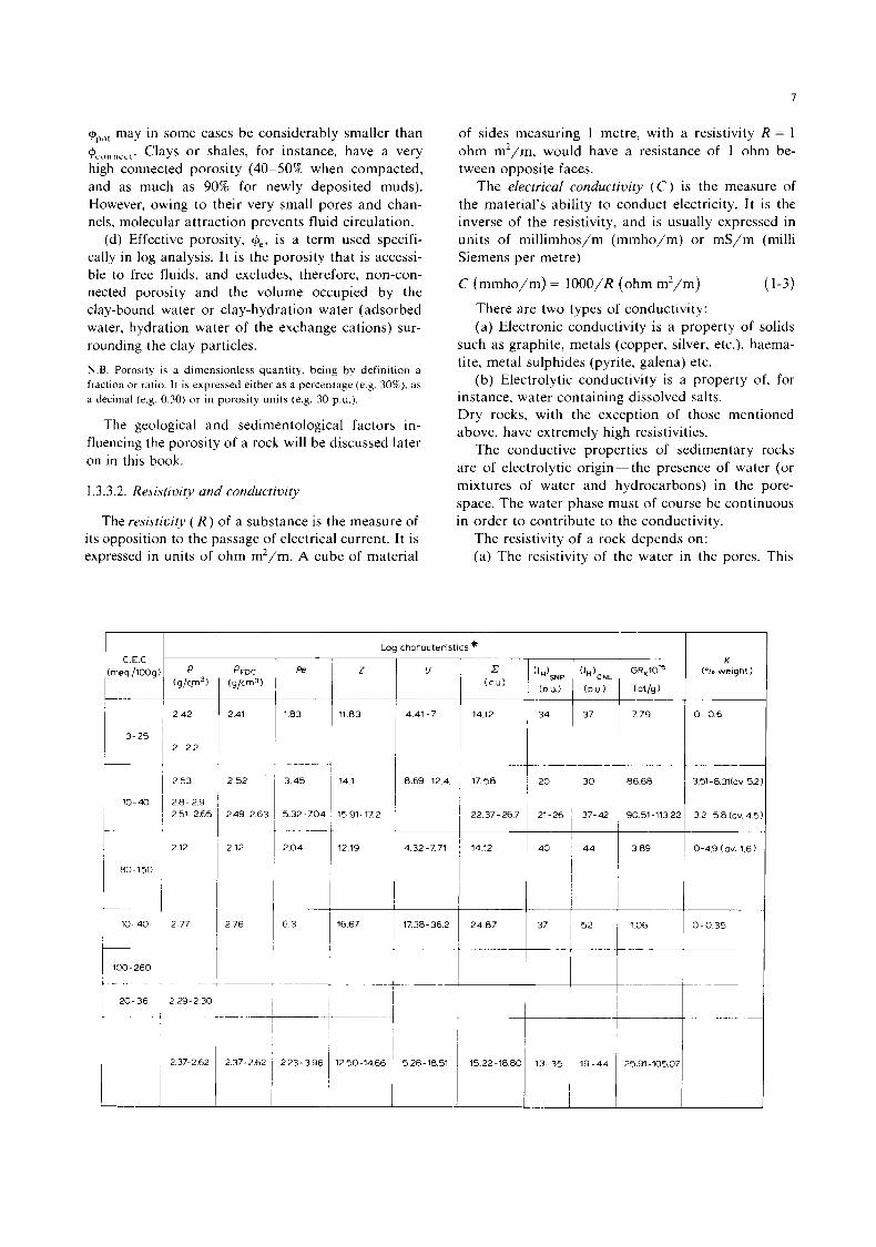
Table 1-1 summarizes the log characteristics (ra- dioactivity, resistivity, hydrogen index, bulk density, acoustic wave velocity . . .) of some of the principle minerals found in sedimentary rocks.
1.3.2. Shale, silt and clay
A shale is a fine-grained, indurated sedimentary rock formed by the consolidation of clay or silt. I t is characterized by a finely stratified structure (laminae 0.1-0.4 mm thick) and/or fissility approximately parallel to the bedding. It normally contains at least 50% silt with, typically, 35% clay or fine mica and 15% chemical or authigenic minerals.
A silt is a rock fragment or detrital particle having a diameter in the range of 1/256 mm to 1/16 mm. I t has commonly a high content of clay minerals associ- ated with quartz, feldspar and heavy minerals such as mica, zircon, apatite, tourmaline, etc.. .
A clay is an extremely fine-grained natural sedi- ment or soft rock consisting of particles smaller than 1/256 mm diameter. I t contains clay minerals (hy- drous silicates, essentially of aluminium, and some- times of magnesium and iron) and minor quantities of finely divided quartz, decomposed feldspars, carbonates, iron oxides and other impurities such as
* For a sedimentologist, matrix is “The smaller or finer-grained, continuous material enclosing, or filling the interstices between the larger grains or particles of a sediment or sedimentary rock; the natural material in which a sedimentary particle is embedded” (Glossary of Geology, A.G.I., 1977).
** For a log analyst, matrix is “all the solid framework of rock which surrounds pore volume”. excluding clay or shale (glossary of terms and expressions used in well logging, S.P.W.L.A.. 1975).
3
i-' r I
4
-N
N
N
00
i .1
00
O
'0
m
N
h
P
m
m
N7
m
*
L
4
- I
TT
'I
II
I
N
W
m
T
c
m Y
5 P 0 I c
5
organic matter. Clays form pasty, plastic impermea- ble masses.
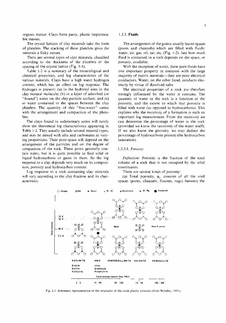
The crystal lattices of clay minerals take the form of platelets. The stacking of these platelets gives the minerals a flaky nature.
There are several types of clay minerals, classified according to the thickness of the platelets or the spacing of the crystal lattice (Fig. 1-1).
Table 1-2 is a summary of the mineralogical and chemical properties, and log characteristics of the various minerals. Clays have a high water hydrogen content, which has an effect on log response. The hydrogen is present: (a) in the hydroxyl ions in the clay mineral molecule; (b) in a layer of adsorbed (or “bound”) water on the clay particle surface; and (c) in water contained in the spaces between the clay platelets. The quantity of this “free-water” varies with the arrangement and compaction of the plate- lets.
The clays found in sedimentary series will rarely show the theoretical log characteristics appearing in Table 1-2. They usually include several mineral types, and may be mixed with silts and carbonates in vary- ing proportions. Their pore-space will depend on the arrangement of the particles and on the degree of compaction of the rock. These pores generally con- tain water, but i t is quite possible to find solid or liquid hydrocarbons or gases in them. So the log response to a clay depends very much on its composi- tion, porosity and hydrocarbon content.
Log response to a rock containing clay minerals will vary according to the clay fraction and its char- acteristics.
1.3.3. Fluids
The arrangement of the grains usually leaves spaces (pores and channels) which are filled with fluids: water, air, gas, oil, tar, etc. (Fig. 1-2). Just how much fluid is contained in a rock depends on the space, or porosity, available.
With the exception of water, these pore-fluids have one important property in common with the large majority of matrix minerals- they are poor electrical conductors. Water, on the other hand, conducts elec- tricity by virtue of dissolved salts.
The electrical properties of a rock are therefore strongly influenced by the water it contains. The quantity of water in the rock is a function of the porosity, and the extent to which that porosity is filled with water (as opposed to hydrocarbons). This explains why the resistivity of a formation is such an important log measurement. From the resistivity we can determine the percentage of water in the rock (provided we know the resistivity of the water itself). If we also know the porosity, we may deduce the percentage of hydrocarbons present (the hydrocarbon saturation).
1.3.3.1. Porosity
Definition: Porosity is the fraction of the total volume of a rock that is not occupied by the solid constituents.
There are several kinds of porosity: (a) Total porosity, $I,, consists of all the void
spaces (pores, channels, fissures, vugs) between the
@OH 0 Silicw 0 Si - A l gAluminlum 0 Al - M Q Potassium
.~ ...
water Water B cations
K A O L I N I T E MICA M O N T M O R I L L O N I l E C H L O R I T E V E R M l C U L l l E
Oick i te l l l i t e Nacr i te G I au con1 te H a l l o y r i t e Pvrophyll i*e
Cation exchange capacity lmeq 1009)
I I I I 3 - 5 I 0 - 00 80 - [I 50 I 0 - 10 100 - 260
Fig. 1 - 1 . Schematic representation of the structures of the main plately minerals (from Brindley. 195 1 ).
h
( H20),
Channel
Grain /
Volcanic ashes
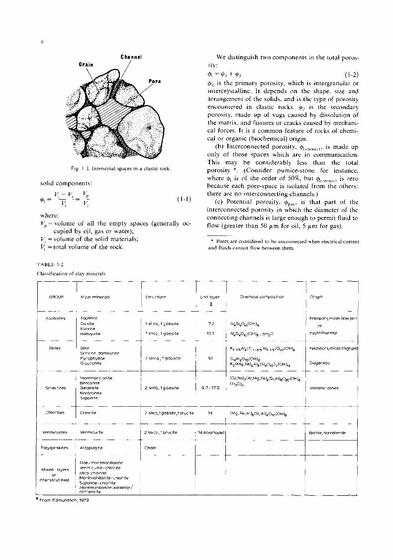
Fig. 1-2. Interstitial spaces in a clastic rock
solid components:
where:
We distinguish two components in the total poros- 1ty:
9, is the primary porosity, which is intergranular or intercrystalline. It depends on the shape, size and arrangement of the solids, and is the type of porosity encountered in clastic rocks. +2 is the secondary porosity, made up of vugs caused by dissolution of the matrix, and fissures or cracks caused by mechani- cal forces. It is a common feature of rocks of chemi- cal or organic (biochemical) origin.
(b) Interconnected porosity, +cconnec,, is made up only of those spaces which are in communication. This may be considerably less than the total porosity *. (Consider pumice-stone for instance, where is of the order of 5056, but +Lii,nnect is zero because each pore-space is isolated from the others: there are no interconnecting channels.)
(c) Potential porosity, GPO,, is that part of the interconnected porosity in which the diameter of the
+t=9, + 9 2 (1-2)
(1-1)
connecting channels is large enough to permit fluid to flow (greater than 50 pm for oil, 5 pm for gas). Vp= volume of all the empty spaces (generally OC-
cupied by oil, gas or water); V, = volume of the solid materials; V, =total volume of the rock.
* Pores are considered to be unconnected when electrical current and fluids cannot flow between them.
T A B L E 1-2
Classification o f clay minerals
GROUP
___ ~
Kaolrnites
Main minerals
Kaolinite Dickite Nacrite Halloysrte
Structure
1 silrca, 1 gibbsite 7 2
1 srlica. 1 gibbsrte I 10 1 I
I
Illites lllite Sericite, darnourite Pyrophyllite Glauconite
2 silica, 1 gibbsite 10
Montmorillonite Bentonite
Nontronite Saponite
Chlorites Chlorite
I 1 2 511im, 1 gibbsite
+. ~
I 2 silica,lgibbsite,l brucite
9.7 - 17 2
14
Mixed -layers o r
interstratif ied
Illite - montrnorillanite Vermiculite - chlorite Mica-chlorite Montmorillonite-chlorite Saponite - chlorite Montrnorillonite-kaolinite/ corrensite
Chemical composition Origin
Feldspars, micas (low pH )
at From Edrnundson, 1979
I 1
I#I~,,[ may in some cases be considerably smaller than q5cconnccl. Clays or shales, for instance, have a very high connected porosity (40-50% when compacted, and as much as 90% for newly deposited muds). However, owing to their very small pores and chan- nels, molecular attraction prevents fluid circulation.
(d) Effective porosity, Ge, is a term used specifi- cally in log analysis. It is the porosity that is accessi- ble to free fluids, and excludes, therefore, non-con- nected porosity and the volume occupied by the clay-bound water or clay-hydration water (adsorbed water, hydration water of the exchange cations) sur- rounding the clay particles. N.B. Porosity is a dimensionless quantity, being by definition a fraction or ratio. I t is expressed either as a percentage (e.g. 30%), as a decimal (e.g. 0.30) or in porosity units (e.g. 30 P.u.).
The geological and sedimentological factors in- fluencing the porosity of a rock will be discussed later on in this book.
of sides measuring 1 metre, with a resistivity R = 1 ohm m2/m, would have a resistance of 1 ohm be- tween opposite faces.
The electrical conductivity (C) is the measure of the material’s ability to conduct electricity. It is the inverse of the resistivity, and is usually expressed in units of millimhos/m (mmho/m) or mS/m (milli Siemens per metre)
C (mmho/m) = IOOO/R (ohm m2/m) (1-3) There are two types of conductivity: (a) Electronic conductivity is a property of solids
such as graphite, metals (copper, silver, etc.), haema- tite, metal sulphides (pyrite, galena) etc.
(b) Electrolytic conductivity is a property of, for instance, water containing dissolved salts. Dry rocks, with the exception of those mentioned above, have extremely high resistivities.
The conductive properties of sedimentary rocks are of electrolytic origin-the presence of water (or mixtures of water and hydrocarbons) in the pore- space. The water phase must of course be continuous in order to contribute to the conductivity.
The resistivity of a rock depends on: (a) The resistivity of the water in the pores. This
1.3.3.2. Resistivitv and conductivity
The resistivity ( R ) of a substance is the measure of its opposition to the passage of electrical current. It is expressed in units of ohm m2/m. A cube of material
Log characteristics i t
K (% weight) P
( g/c.m3) Pe
183
3 45
5 32-704
2 42
2 - 2 2
2.41 37 7 79
86 68
90 51-113 2.
0 - 0 6
. . ._ - . -
351-831(av 5;
32-58(av4E
1 34 11.83 1 4.41-7 1 14.12
2.53
2.8 - 2.9 2.51 -2.65
2 52
249-263
2 12
30
37- 42
141 1 8 6 9 - 1 2 4 1 1 7 5 8 20
1 I 21-26
15 91-17 2 1 2237-267 ’ 1 ’ 10-40
t 212
1 80-150
I ! 432-7.71 i 14.12
~ ~ ~ ~ ~ I I I
I ! 40
2.04 1 12.19 44 3.89 0-4.9 (OV. 1.6)
~
0 - 0 3 5 -+-- 52 2.76
-
1 10-40
100 - 260
l 20-36
2 77 6 3 ~ 1667 1 1738-362 1 2487 1 37
1
2 29-2 30
I- --!
X
will vary with the nature and concentration of its dissolved salts.
(b ) The quantity of water present; that is, the porosity and the saturation.
(c) Lithology, i.e. the nature and percentage of clays present, and traces of conductive minerals.
( d ) The texture of the rock; i.e. distribution of pores, clays and conductive minerals.
(e ) The temperature. Resistivity may be anisotropic by virtue of stratifi-
cation (layering) in the rock, caused, for instance, by deposition of elongated or flat particles. oriented in the direction of a prevailing current. This creates preferential paths for current flow (and fluid move- ment), and electrical conductivity is not the same in all directions.
We define horizontal resistivity ( R,) in the direc- tion of layering, and vertical resistivity ( R , ) per- pendicular to this.
The anisotropy coefficient, A , is:
x = ( R, /R{ i )1’2 ( 1-4)
This can vary between 1.0 and 2.5, with R, generally larger than R,. It is R, that we measure with the laterolog and other resistivity tools (induction), whereas the classical electrical survey reads some- where between R,, and R,.
The mean resistivity of an anisotropic formation is:
R = ( R , , R , ) ” ’ (1-5) The anisotropy of a single uniform layer is micro-
scopic anisotropy. When we talk of the overall char- acteristic of a sequence of thin resistive layers, this is inacroscopic anisotropy. In such a series, the current tends to flow more easily along the layers than across them, and this anisotropy will affect any tool reading resistivity over a volume of formation containing these fine layers.
Microscopic anisotropy occurs in clays, and mud- cakes. In the second case, the resistivity measured through the mudcake perpendicular to the wall of the hole is higher than that parallel to the axis. This has an effect on the focussed micro-resistivity tools (MLL, PML) which must be taken into account in their interpretation. A mud-cake of anisotropy, A, and thickness, h mc, is electrically equivalent to an iso- tropic mud-cake having a resistivity equal to the mean, R,,Rv with thickness, Ah,,,.
Summarizing, what we call the true resistivity ( R , ) o f a formation is a resistivity dependent on the fluid content and the nature and configuration of the solid matrix.
1.3.3.2.1, The relurionship between resistivity and salin- i p
We have mentioned that the resistivity of an elec-
0 100 000 290 O00 400 000
CONCENTRATION - PPM
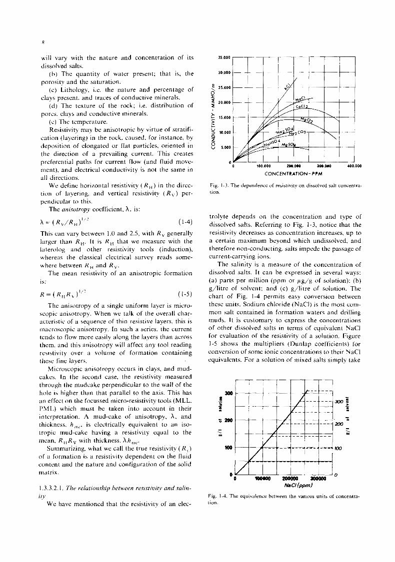
Fig. 1-3. The dependence of resistivity on dissolved salt concentra- tion.
trolyte depends on the concentration and type of dissolved salts. Referring to Fig. 1-3, notice that the resistivity decreases as concentration increases, up to a certain maximum beyond which undissolved, and therefore non-conducting, salts impede the passage of current-carrying ions.
The salinity is a measure of the concentration of dissolved salts. It can be expressed in several ways: (a) parts per million (ppm or pg/g of solution); (b) g/litre of solvent; and (c) g/litre of solution. The chart of Fig. 1-4 permits easy conversion between these units. Sodium chloride (NaCI) is the most com- mon salt contained in formation waters and drilling muds. It is customary to express the concentrations of other dissolved salts in terms of equivalent NaCl for evaluation of the resistivity of a solution. Figure 1-5 shows the multipliers (Dunlap coefficients) for conversion of some ionic concentrations to their NaCl equivalents. For a solution of mixed salts simply take
Na CI bpm)
Fig. 1-4. The equivalence between the various units of concentra- tion.
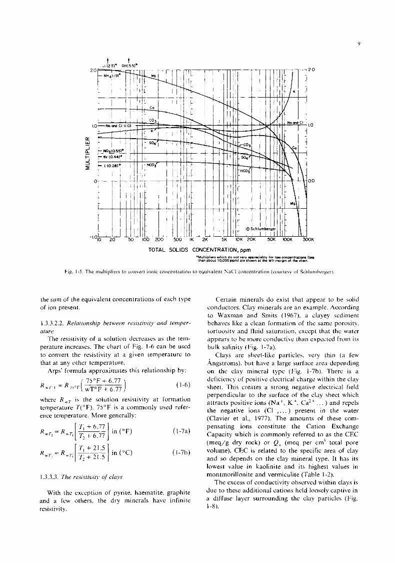
9
TOTAL SOLIDS CONCENTRATION, ppm 'Multipliers which do not vary appreciably for low concentrations I I S n than abwt 10.000 ppm) are shown et the left margin of the chart.
Fig. 1-5. The multipliers to convert ionic concentration to equivalent NaCl concentration (courtesy o f Schlumhrrgrr)
the sum of the equivalent concentrations of each type of ion present.
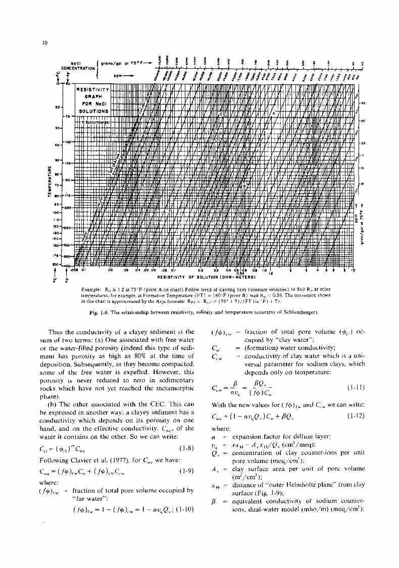
1.3.3.2.2. Relutionship between resistivity und temper- ature
The resistivity of a solution decreases as the tem- perature increases. The chart of Fig. 1-6 can be used to convert the resistivity at a given temperature to that at any other temperature.
Arps' formula approximates this relationship by:
where R,, is the solution resistivity at formation temperature T("F) . 75°F is a commonly used refer- ence temperature. More generally:
TI + 21.5 R,,, = Rw,,
( 1 -7a)
( 1 -7b)
1.3.3.3. The resistivity of duys
With the exception of pyrite, haematite. graphite and a few others. the dry minerals have infinite resistivity.
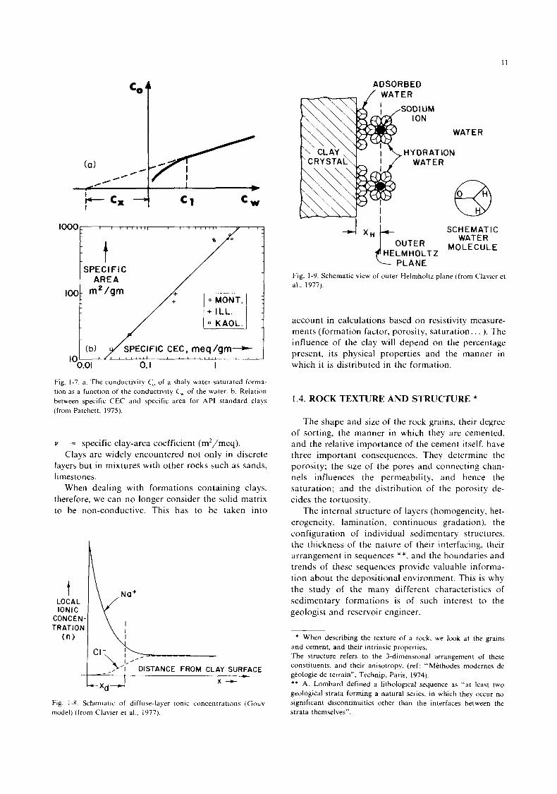
Certain minerals do exist that appear to be solid conductors. Clay minerals are an example. According to Waxman and Smits (1967), a clayey sediment behaves like a clean formation of the same porosity. tortuosity and fluid saturation, except that the water appears to be more conductive than expected from its bulk salinity (Fig. 1-7a).
Clays are sheet-like particles, very thin (a few Angstroms), but have a large surface area depending on the clay mineral type (Fig. 1-7b). There is a deficiency of positive electrical charge within the clay sheet. This creates a strong negative electrical field perpendicular to the surface of the clay sheet which attracts positive ions (Na+, K+, Ca*+. . . ) and repels the negative ions (Cl-, . . .) present in the water (Clavier et al., 1977). The amounts of these com- pensating ions constitute the Cation Exchange Capacity which is commonly referred to as the CEC (meq/g dry rock) or Q , (meq per cm' total pore volume). CEC is related to the specific area of clay and so depends on the clay mineral type. It has its lowest value in kaolinite and its highest values in montmorillonite and vermiculite (Table 1-2).
The excess of conductivity observed within clays i s due to these additional cations held loosely captive in a diffuse layer surrounding the clay particles (Fig. 1-8).
10
' I ! I .02 .Ob .$4 .dS .do ' .d@ d.1 0.2 d! d4 dd I d8 O$ ' II.0 I
0.68 1.1 RESISTIVITY OF SOLUTION (OHM-METERS)
2 0 " Example: R, is 1.2 at 75$F (point A on chart). Follow trend of slanting lines (constant salinities) to find R, at other temperatures; for example, at Formation Temperature (FT) = 160'F (point B ) read R, = 0.56. The conversion shown in rhis chart is approximated by the Arps formula: RFT = R7,. x ( 7 5 " + 7) / (FT (in 'F) + 7) .
Fig. 1-6. The relationship between resistivity, salinity and temperature (courtesy of Schlumberger).
Thus the conductivity of a clayey sediment is the sum of two terms: (a) One associated with free water or the water-filled porosity (indeed this type of sedi- ment has porosity as high as 80% at the time of deposition. Subsequently, as they become compacted, some of the free water is expelled. However, this porosity is never reduced to zero in sedimentary rocks which have not yet reached the metamorphic phase).
(b ) The other associated with the CEC. This can be expressed in another way: a clayey sediment has a conductivity which depends o n its porosity on one hand, and o n the effective conductivity, C,,, of the water it contains on the other. So we can write:
c,, = (+,,,>"'Cw, (1-8)
c,, = (f+)rwCw + (f+)cwcc, (1-9)
Following Clavier et al. (1977), for C,, we have:
where: ( = fraction of total pore volume occupied by
"far water":
( f + ) f w = l - ( f + ) c w = l - a o q Q v ; (1-10)
fraction of total pore volume ( + c , ) oc- cupied by "clay water"; (formation) water conductivity; conductivity of clay water which is a uni- versal parameter for sodium clays, which depends only on temperature:
(1 -11)
With the new values for (f+),, and C,, we can write:
cw, = ( 1 - w&>~, + PQ, (1-12)
where: a =
- *q - Q , =
A,, =
X H =
P =
expansion factor for diffuse layer; v x H = A v x H / Q v (cm-'/meq); concentration of clay counter-ions per unit pore volume (meq/cm3 1: clay surface area per unit of pore volume (m2/cm3 ); distance of "outer Helmholtz plane" from clay surface (Fig. 1-9); equivalent conductivity of sodium counter- ions, dual-water model (mho/m) (meq/cm3);
I 1
ADSORBED
WATER ‘I C 1 C W
SPEC1 F I C I o o o 1 / AREA
I (b), /SPECIFIC CEC, meq/gm- t 1 # 1 1 1 1 1
‘O0.Ol 0. I I
Fig. 1-7. a. The conductivity C,, of a shaly water-saturated forma- tion as a function of the conductivity C,, of the water. b. Relation between specific CEC and specific area for API standard clays (from Patchett. 1975).
v Clays are widely encountered not only in discrete
layers but in mixtures with other rocks such as sands, limes tones.
When dealing with formations containing clays, therefore, we can no longer consider the solid matrix to be non-conductive. This has to be taken into
= specific clay-area coefficient (m2/meq>.
CONCEN- TRATION
( n )
-
x - +
Fig. I - X . Schcmatlc o f diffuse-layer mnic concentratlons (Gouv model) (from Clavier et al.. 1977).
SCHEMATIC WATER
OUTER MOLECULE HELM HOLT Z ‘-- PLANE
Fig. 1-9. Schematic view of outer Helmholtz plane (from Clavier et al.. 1977).
account in calculations based on resistivity measure- ments (formation factor, porosity, saturation.. . ). The influence of the clay will depend on the percentage present, its physical properties and the manner in which it is distributed in the formation.
1.4. ROCK TEXTURE AND STRUCTURE *
The shape and size of the rock grains, their degree of sorting, the manner in which they are cemented. and the relative importance of the cement itself. have three important consequences. They determine the porosity; the size of the pores and connecting chan- nels influences the permeability, and hence the saturation; and the distribution of the porosity de- cides the tortuosity.
The internal structure of layers (homogeneity, het- erogeneity, lamination, continuous gradation). the configuration of individual sedimentary structures, the thickness of the nature of their interfacing, their arrangement in sequences **, and the boundaries and trends of these sequences provide valuable informa- tion about the depositional environment. This is why the study of the many different characteristics of sedimentary formations is of such interest to the geologist and reservoir engineer.
* When describing the texture of a rock. we look at the grains and cement, and their intrinsic properties. The structure refers to the 3-dimensional arrangement of these constituents, and their anisotropy. (ref: “ Methodes modernes de geologie de terrain”, Technip, Paris, 1974). * * A. Lombard defined a lithological sequence as “at least two geological strata forming a natural series. in which they occur no significant discontinuities other than the interfaces between the strata themselves”.
12
Face A .
Fig. 1-10, Theoretical case-a cube of unit volume containing parallel cylindrical capillaries of cross-sectional area So.
Well-log interpretation will provide much of this information. Before embarking on a detailed study of how this is achieved, we must understand the basic relationships between the log measurements and the physical parameters.
1.4.1. The relationship between porosity and resistiv- ity: the formation factor
In clean, porous aquifers, the formation resistivity R, , is proportional to that of the interstitial water,
R,, = F , R w (I-13a)
F , is the formation resistivity factor, a function of the rock texture. It is the ratio of the resistivity of the formation to that of the water with which i t is 100%
R,:
saturated:
FR = R , / R w (1-l3b)
If the interstitial spaces were made up solely of parallel cylindrical channels (Fig. 1-10), R , would be inversely proportional to the porosity. The resistance between faces A and B of the elementary cube of Fig. 1-10 is, by definition: R , = R, - I
S P (1-14)
Sp being the cross-sectional area of each of the chan- nels. Now Sp is equal to + t :
“P 1 x s, + =-=(seesection I .3.3.I .)= ‘ K I X l X l
= s, ( / = 1 ) (1-15)
S o : R = R,+/+(, which means that F , = I / + ( . In reality, the electrical current is constrained to
follow complex meandering paths, whose lengths in- crease with their tortuosity. and whose sectional areas (and hence resistances) vary erratically between the pores and fine interconnecting capillaries. The nature of these paths depends on the rock texture.
A large number of measurements on rock samples has shown that the formation factor of a shale-free rock is related reasonably consistently to porosity by:
FR = a/+”‘ (1-16)
u is a coefficient between 0.6 and 2.0 depending on
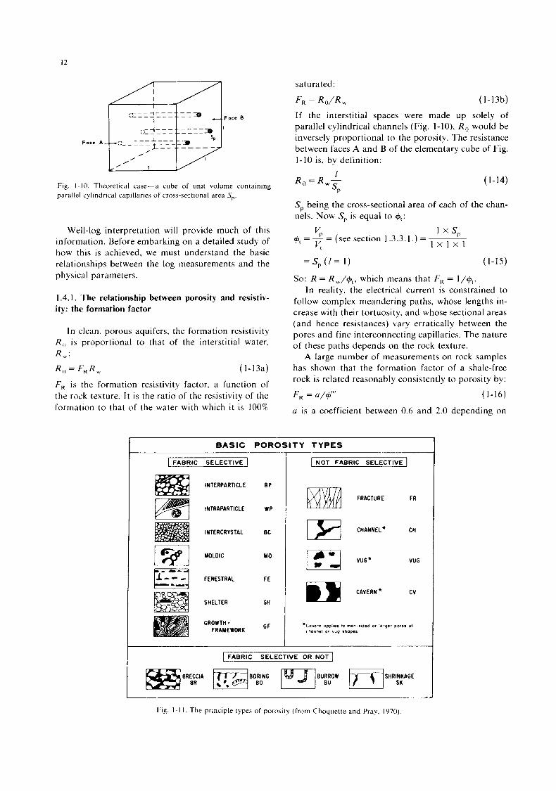
BASIC POROSITY TYPES
I FABRIC SELECTIVE I
INTERPARTICLE
MOLDIC w SHELTER
E P
WP
BC
MO
FE
SH
GF
I NOT FABRIC SELECTIVE I
FRACTURE FR
CHANNEL‘ CH
r A VUG” VUG
*Cavern opphes lo men stred or lnrgsr pores of channel or vug rnapss
I FABRIC SELECTIVE OR NOT 1
Fig. 1-1 I . The principle types of porosity (from Choquette and Pray. 1970)
13
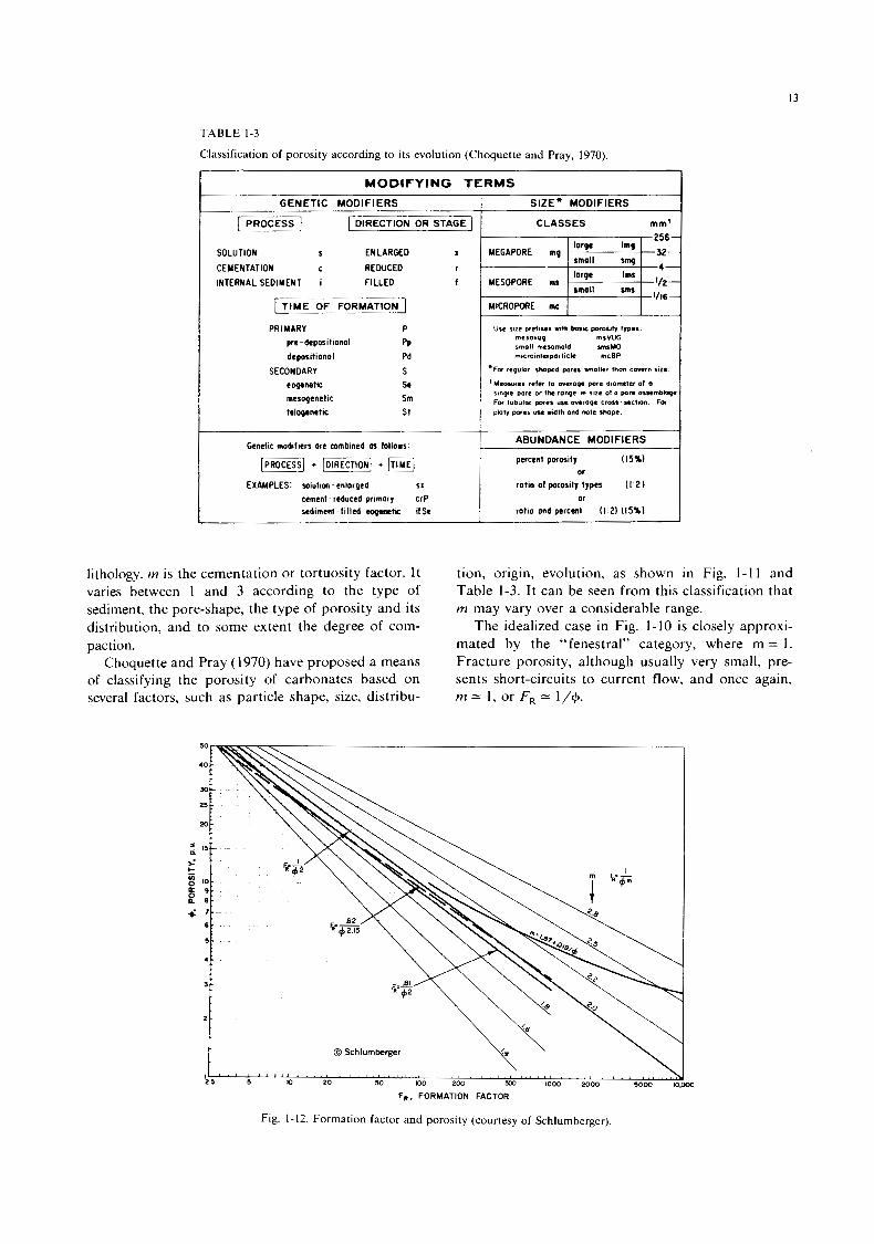
TABLE 1-3
Classification of porosity according to its evolution (Choquette and Pray, 1970).
I MODIFYING TERMS
GENETIC MODIFIERS
lpizEEq I DIRECTION OR STAGE 1 SOLUTION S ENLARGED I
CEMENTATION C REDUCED r
INTERNAL SEDIMENT i FILLED f
[ T I M E OF FORMATION
PRIMARY P
pre -depositional PP
SECONDARY S eop.wtic SI
telogenetic Sl
depositional Pd
mesogenetic Sm
Genetic modiliers OR combined m follows
[PROCESS] + pzEiq +[TIME] EXAMPLES- solulion -enlarged S I
cement -reduced primary CrP sediment-filled eogomlr if%
SIZE” MODIFIERS
CLASSES mmt
ABUNDANCE MODIFIERS
percent porosity (15x1 or
ratio of porosity types
rotio and percent
(I 2 1
(I 21 (15%) or
lithology. m is the cementation or tortuosity factor. I t tion, origin, evolution, as shown in Fig. 1-1 1 and -.. varies between 1 and 3 according to the type of sediment, the pore-shape, the type of porosity and its distribution, and to some extent the degree of com- paction.
Choquette and Pray (1970) have proposed a means of classifying the porosity of carbonates based on several factors, such as particle shape, size, distribu-
Table 1-3. It can be seen from this classification that in may vary over a considerable range.
The idealized case in Fig. 1-10 is closely approxi- mated by the “fenestral” category, where m = 1. Fracture porosity, although usually very small, pre- sents short-circuits to current flow, and once again, in = 1, or FR = I/+.
Fig. 1-12. Formation factor and porosity (courtesy of Schlumberger)
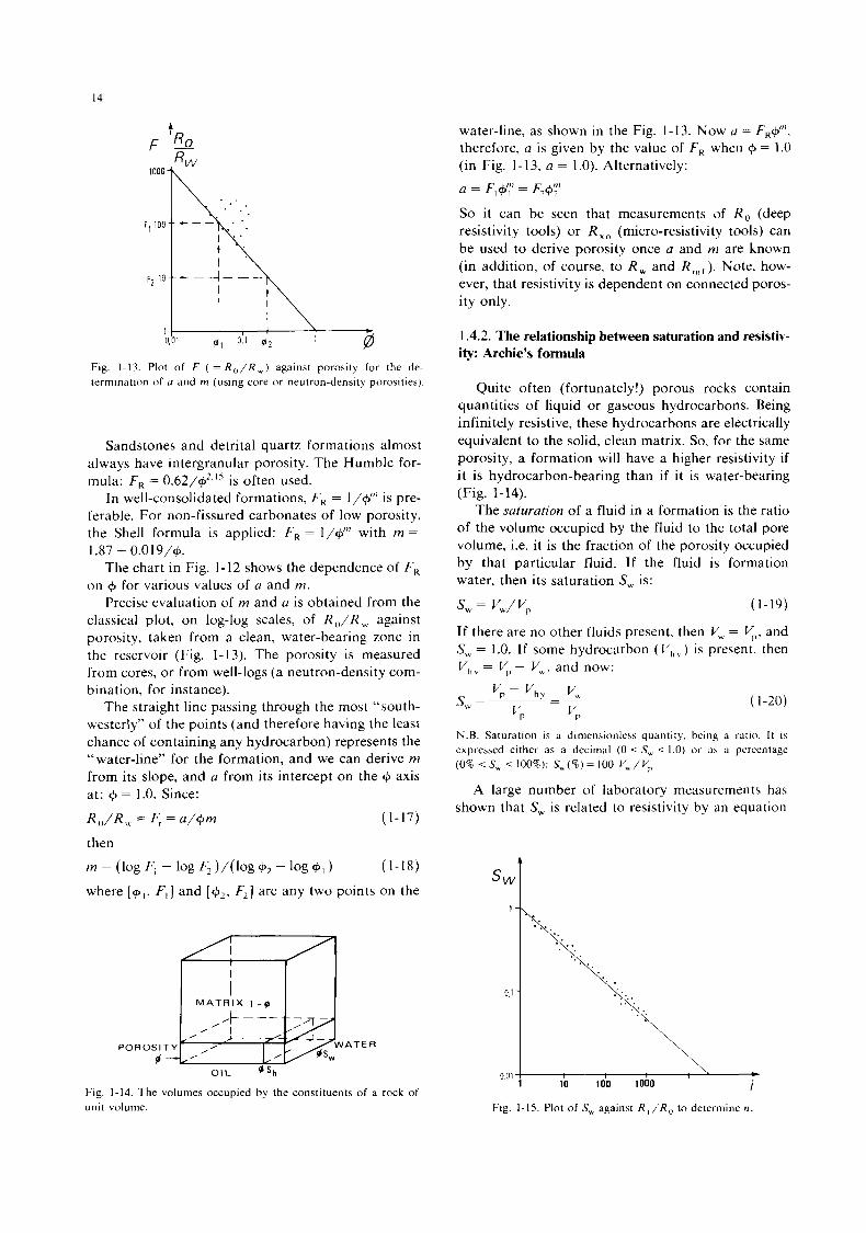
14
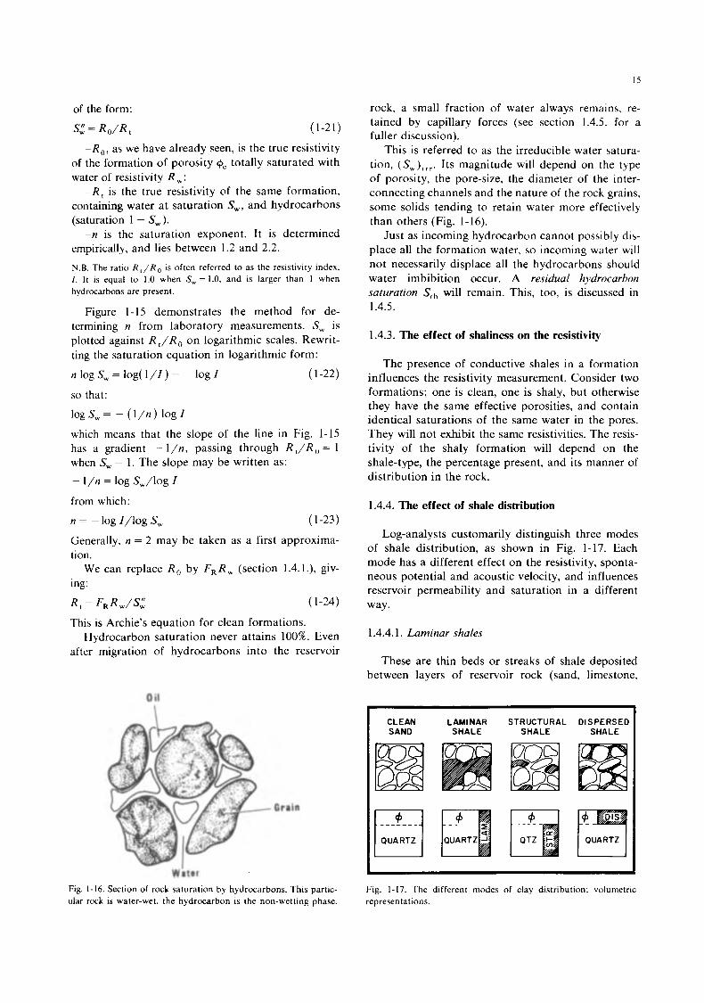
A F = + ‘ R
Fig. 1-13. Plot of F ( = R , , / R , ) against porosity for the de- termination of u and m (using core or neutron-density porosities).
Sandstones and detrital quartz formations almost always have intergranular porosity. The Humble for- mula: F , = 0.62/G2.I5 is often used.
In well-consolidated formations, F, = I/+’” is pre- ferable. For non- fissured carbonates of low porosity, the Shell formula is applied: F, = I/+’” with m =
1.87 + 0.0 19/+. The chart in Fig. 1-12 shows the dependence of F ,
on + for various values of a and m. Precise evaluation of m and a is obtained from the
classical plot, on log-log scales, of R, , /R , against porosity, taken from a clean, water-bearing zone in the reservoir (Fig. 1-13). The porosity is measured from cores, or from well-logs (a neutron-density com- bination, for instance).
The straight line passing through the most “south- westerly” of the points (and therefore having the least chance of containing any hydrocarbon) represents the “water-line’’ for the formation, and we can derive m from its slope, and a from its intercept on the $ axis at: $ = 1.0. Since:
R , , / R , = F, = u/+m (1-17)
then m = (log F, -
where [+,, F,
1% F2 )/(log $2 - 1% $ 1 ) (1-18)
and [&, F2] are any two points on the
Fig. 1-14. The volumes occupied by the constituents of a rock of unit volume.
water-line, as shown in the Fig. 1-13. Now a = FR$‘”. therefore, a is given by the value of F , when @ = 1.0 (in Fig. 1-13, a = 1.0). Alternatively: a = Fl+’;’ = F +I” 2 2
So it can be seen that measurements of R , (deep resistivity tools) or R x o (micro-resistivity tools) can be used to derive porosity once a and m are known (in addition, of course, to R , and R, , f ) . Note, how- ever, that resistivity is dependent on connected poros- ity only.
1.4.2. The relationship between saturation and resistiv- ity: Archie’s formula
Quite often (fortunately!) porous rocks contain quantities of liquid or gaseous hydrocarbons. Being infinitely resistive, these hydrocarbons are electrically equivalent to the solid, clean matrix. So, for the same porosity, a formation will have a higher resistivity if it is hydrocarbon-bearing than if it is water-bearing (Fig. 1-14).
The saturation of a fluid in a formation is the ratio of the volume occupied by the fluid to the total pore volume, i.e. it is the fraction of the porosity occupied by that particular fluid. If the fluid is formation water, then its saturation S, is:
s, = V,/V, (1-19)
If there are no other fluids present, then V,, = V,. and S, = 1 .O. If some hydrocarbon ( V,, ) is present, then Vl,v = V, - V,, and now:
( 1-20)
N.B. Saturation is a dimensionless quantity, being a ratio. I t is expressed either as a decimal (0 < S, < 1.0) o r as a percentage (0% < S, < 100%): S,(%) = 100 v,,,/v,
A large number of laboratory measurements has shown that S, is related to resistivity by an equation
swl
Fig. 1-15. Plot of S,,, against R , / R , to determine n
15
of the form: S: = R , / R , (1-21)
- R 0 , as we have already seen, is the true resistivity of the formation of porosity +e totally saturated with water of resistivity R , :
- R , is the true resistivity of the same formation, containing water at saturation S,, and hydrocarbons (saturation 1 - Sw).
-n is the saturation exponent. It is determined empirically, and lies between 1.2 and 2.2. N.B. The ratio R , / R , , is often referred to as the resistivity index, I. It is equal to 1.0 when S, = 1.0, and is larger than 1 when hydrocarbons are present.
Figure 1-15 demonstrates the method for de- termining n from laboratory measurements. S, is plotted against R , / R 0 on logarithmic scales. Rewrit- ting the saturation equation in logarithmic form:
n log s, = log( 1 / 1 ) = -log z
log s, = - (1 /n) log I
( 1-22)
so that:
which means that the slope of the line in Fig. 1-15 has a gradient - l /n, passing through R , / R o = 1 when S, = 1. The slope may be written as: - I /n = log S,/log I
from which:
n = - log I/log s , ( 1-23)
Generally, n = 2 may be taken as a first approxima- tion.
We can replace R , by F , R , (section 1.4.1.), giv- ing:
R , = F , R ,/St ( 1-24)
This is Archie’s equation for clean formations. Hydrocarbon saturation never attains 100%. Even
after migration of hydrocarbons into the reservoir
0 il
Grain
W i t t r
Fig. 1-16. Section of rock saturation by hydrocarbons. This partic- ular rock is water-wet, the hydrocarbon is the non-wetting phase.
rock, a small fraction of water always remains, re- tained by capillary forces (see section 1.4.5. for a fuller discussion).
This is referred to as the irreducible water satura- tion, (S,),,,. Its magnitude will depend on the type of porosity, the pore-size, the diameter of the inter- connecting channels and the nature of the rock grains, some solids tending to retain water more effectively than others (Fig. 1-16).
Just as incoming hydrocarbon cannot possibly dis- place all the formation water, so incoming water will not necessarily displace all the hydrocarbons should water imbibition occur. A residual hydrocarbon saturation S,, will remain. This, too, is discussed in 1.4.5.
1.4.3. The effect of shaliness on the resistivity
The presence of conductive shales in a formation influences the resistivity measurement. Consider two formations; one is clean, one is shaly, but otherwise they have the same effective porosities, and contain identical saturations of the same water in the pores. They will not exhibit the same resistivities. The resis- tivity of the shaly formation will depend on the shale-type, the percentage present, and its manner of distribution in the rock.
1.4.4. The effect of shale distribution
Log-analysts customarily distinguish three modes of shale distribution, as shown in Fig. 1-17. Each mode has a different effect on the resistivity, sponta- neous potential and acoustic velocity, and influences reservoir permeability and saturation in a different way.
1.4.4.1. Laminar shales
These are thin beds or streaks of shale deposited between layers of reservoir rock (sand, limestone,
CLEAN LAMINAR STRUCTURAL DISPERSED I SAND SHALE SHALE SHALE
Fig. 1-17. The different modes of clay distribution; volumetric representations.
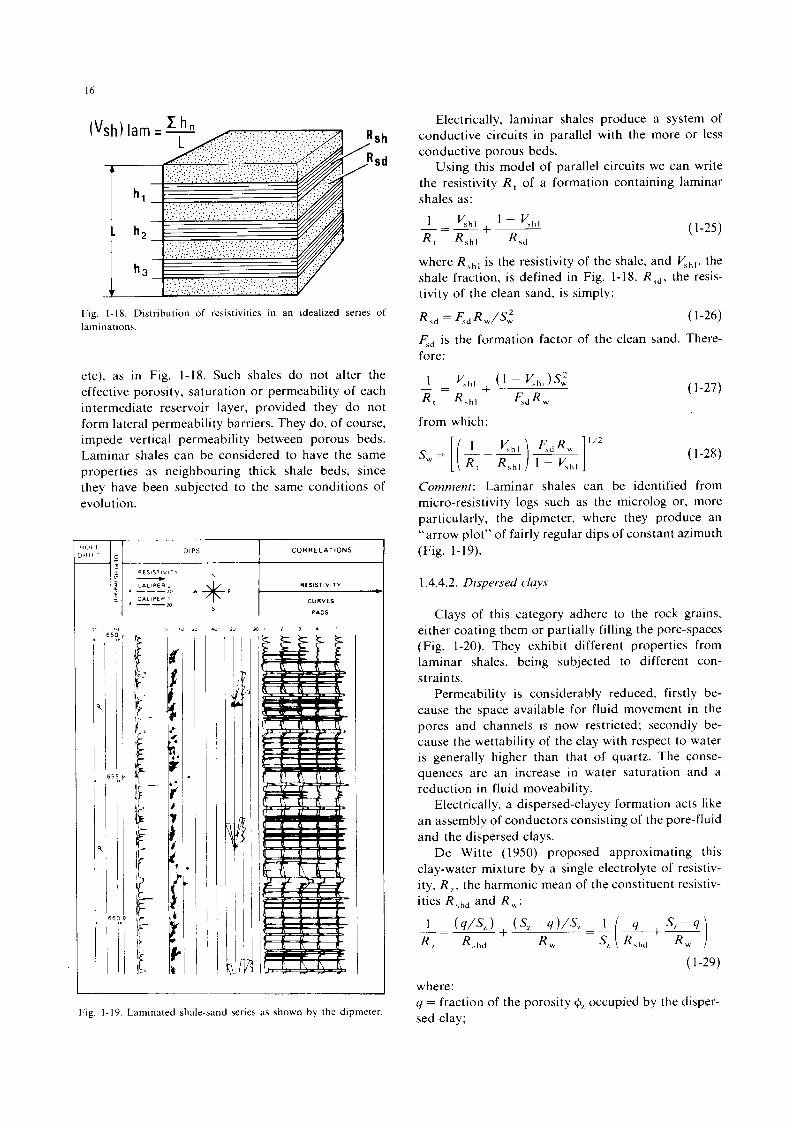
16
Fig. 1-18. Distribution of resistivities in an idealized series of laminations.
etc), as in Fig. 1-18. Such shales do not alter the effective porosity, saturation or permeability of each intermediate reservoir layer, provided they do not form lateral permeability barriers. They do, of course, impede vertical permeability between porous beds. Laminar shales can be considered to have the same properties as neighbouring thick shale beds, since they have been subjected to the same conditions of evolution.
DIPS I CORRELATIONS
S
."- I CURVES
PADS
mJ 9 0 1 i 1 . I
Fig. 1-19. Laminated shale-sand series as shown by the dipmeter.
Electrically, laminar shales produce a system of conductive circuits in parallel with the more or less conductive porous beds.
Using this model of parallel circuits we can write the resistivity R , of a formation containing laminar shales as:
(1-25)
where R,,, is the resistivity of the shale, and Y h l , the shale fraction, is defined in Fig. 1-18. R,,, the resis- tivity of the clean sand, is simply:
R,, = <,R,/s: ( 1-26)
5, is the formation factor of the clean sand. There- fore:
from which:
( 1-27)
( 1-28)
Comment: Laminar shales can be identified from micro-resistivity logs such as the microlog or, more particularly, the dipmeter, where they produce an "arrow plot" of fairly regular dips of constant azimuth (Fig. 1-19).
1.4.4.2. Dispersed clays
Clays of this category adhere to the rock grains, either coating them or partially filling the pore-spaces (Fig. 1-20). They exhibit different properties from laminar shales, being subjected to different con- straints.
Permeability is considerably reduced. firstly be- cause the space available for fluid movement in the pores and channels is now restricted; secondly be- cause the wettability of the clay with respect to water is generally higher than that of quartz. The conse- quences are an increase in water saturation and a reduction in fluid moveability.
Electrically, a dispersed-clayey formation acts like an assembly of conductors consisting of the pore-fluid and the dispersed clays.
De Witte (1950) proposed approximating this clay-water mixture by a single electrolyte of resistiv- ity, R,, the harmonic mean of the constituent resistiv- ities R,,, and R,:
1 - ( 4 / S , ) + (S, - 4 ) / S , - - 1 __
R7 R,hd R u s, i R,hd +'"'I R ,
( 1-29)
where: q = fraction of the porosity +, occupied by the disper- sed clay;
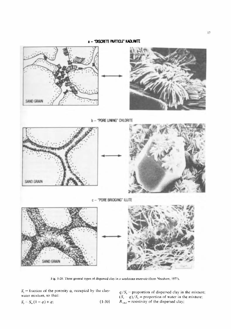
-3
L1
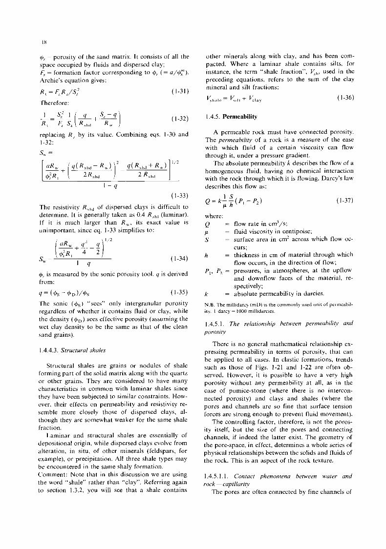
+, = porosity of the sand matrix. I t consists of all the space occupied by fluids and dispersed clay; F, = formation factor corresponding to += ( = a/+;). Archie’s equation gives:
R , = F,R, / s ,Z (1-31)
Therefore:
( 1-32)
replacing R , by its value. Combining eqs. 1-30 and 1-32: s, =
I - q (1-33)
The resistivity R,,,d of dispersed clays is difficult to determine. I t is generally taken as 0.4 R,,, (laminar). I f i t is much larger than R,. its exact value is unimportant, since eq. 1-33 simplifies to:
( 1-34)
+, is measured by the sonic porosity tool. q is derived from: y = ( + s - + o ) / + s ( 1-35)
The sonic ( +s) “sees” only intergranular porosity regardless of whether it contains fluid or clay, while the density (+,,) sees effective porosity (assuming the wet clay density to be the same as that of the clean sand grains).
1.4.4.3. Structural shales
Structural shales are grains or nodules of shale forming part of the solid matrix along with the quartz or other grains. They are considered to have many characteristics in common with laminar shales since they have been subjected to similar constraints. How- ever, their effects on permeability and resistivity re- semble more closely those of dispersed clays, al- though they are somewhat weaker for the same shale fraction.
Laminar and structural shales are essentially of depositional origin, while dispersed clays evolve from alteration, in situ, of other minerals (feldspars, for example), or precipitation. All three shale types may be encountered in the same shaly formation. Comment: Note that in this discussion we are using the word “shale” rather than “clay”. Referring again to section 1.3.2, you will see that a shale contains
other minerals along with clay, and has been com- pacted. Where a laminar shale contains silts, for instance, the term “shale fraction”, Yhr used in the preceding equations, refers to the sum of the clay mineral and silt fractions:
1.4.5. Permeability
( 1-36)
A permeable rock must have connected porosity. The permeability of a rock is a measure of the ease with which fluid of a certain viscosity can flow through it, under a pressure gradient.
The absolute permeability k describes the flow of a homogeneous fluid, having no chemical interaction with the rock through which it is flowing. Darcy’s law describes this flow as:
1 s Q = k - - ( P , - P 2 )
P h (1-37)
where: Q = flow rate in cm3/s; P = fluid viscosity in centipoise; S = surface area in cm2 across which flow OC-
curs; h = thickness in cm of material through which
flow occurs, in the direction of flow; P I , Pz = pressures, in atmospheres, at the upflow
and downflow faces of the material, re- spectively;
k = absolute permeability in darcies. N.B. The millidarcy (mD) is the commonly used unit o f permeabil- ity. 1 darcy = 1000 millidarcies.
1.4.5.1. The relationship between permeabilitv and porosity
There is no general mathematical relationship ex- pressing permeability in terms of porosity, that can be applied to all cases. In clastic formations, trends such as those of Figs. 1-21 and 1-22 are often ob- served. However, i t is possible to have a very high porosity without any permeability at all, as in the case of pumice-stone (where there is no intercon- nected porosity) and clays and shales (where the pores and channels are so fine that surface tension forces are strong enough to prevent fluid movement).
The controlling factor, therefore, is not the poros- ity itself, but the size of the pores and connecting channels, if indeed the latter exist. The geometry of the pore-space, in effect, determines a whole series of physical relationships between the solids and fluids of the rock. This is an aspect of the rock texture.
1.4.5.1.1. Contact phenomena between water and rock - capillarity
The pores are often connected by fine channels of
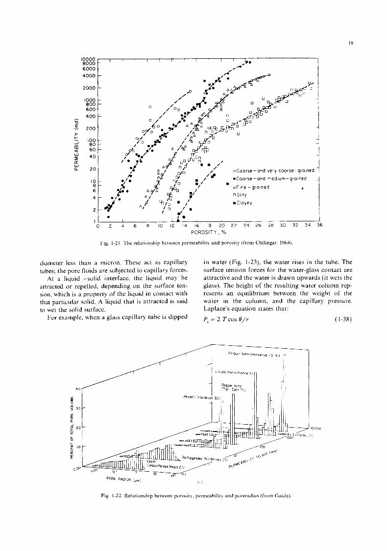
19
Fig. 1-21, The relationship between permeability and porosity (from Chilingar. 1964)
diameter less than a micron. These act as capillary tubes; the pore fluids are subjected to capillary forces.
At a liquid-solid interface, the liquid may be attracted or repelled, depending on the surface ten- sion, which is a property of the liquid in contact with that particular solid. A liquid that is attracted is said to wet the solid surface.
For example, when a glass capillary tube is dipped
in water (Fig. 1-23), the water rises in the tube. The surface tension forces for the water-glass contact are attractive and the water is drawn upwards ( i t wets the glass). The height of the resulting water column rep- resents an equilibrium between the weight of the water in the column, and the capillary pressure. Laplace's equation states that: P, = 2 T cos e / r ( 1-38)
4 0 / w q 2 20
B
k 0 Po'
Fig. 1-22. Relationship between porosity, permeability and poreradius (from Gaida).
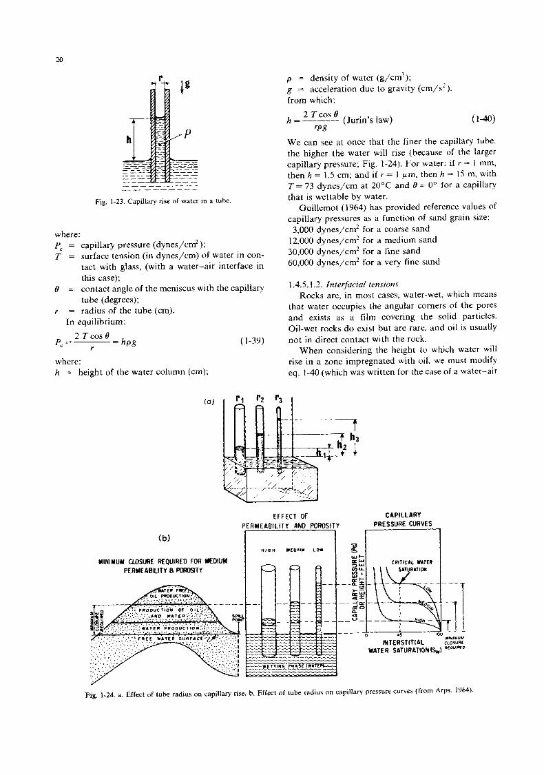
20
- - - - - - - - - - - - - - - - - - - Fig. 1-23. Capillary rise of water in a tube.
where: P, = capillary pressure (dynes/cm2); T = surface tension (in dynes/cm) of water in con-
tact with glass, (with a water-air interface in this case);
= contact angle of the meniscus with the capillary tube (degrees);
0
r = radius of the tube (cm). In equilibrium:
2 Tcosb' P, = = hpg
Y
where: h = height of the water column (cm);
( 1-39)
p = density of water (g/cm3); g = acceleration due to gravity (cm/s2). from whch:
h = 2 Tcos 8 (Jurin's law) ( 1-40)
We can see at once that the finer the capillary tube, the higher the water will rise (because of the larger capillary pressure; Fig. 1-24). For water: if r = 1 mm, then h = 1.5 cm; and if r = 1 pm, then h = 15 m, with T = 73 dynes/cm at 20°C and 0 = 0" for a capillary that is wettable by water.
Guillemot (1 964) has provided reference values of capillary pressures as a function of sand grain size:
3,000 dynes/cm2 for a coarse sand 12,000 dynes/cm2 for a medium sand 30,000 dynes/cm2 for a fine sand 60,000 dynes/cm2 for a very fine sand
rPg
1.4.5.1.2. Interfacial tensions Rocks are, in most cases, water-wet, which means
that water occupies the angular corners of the pores and exists as a film covering the solid particles. Oil-wet rocks do exist but are rare, and oil is usually not in direct contact with the rock.
When considering the height to which water will rise in a zone impregnated with oil, we must modify eq. 1-40 (which was written for the case of a water-air
t
EFFECT OF CAPILLARY
Fig. 1-24. a. Effect of tube radius on capillary rise. b. Effect of tube radius on capillary pressure curves (from Arps, 1964).
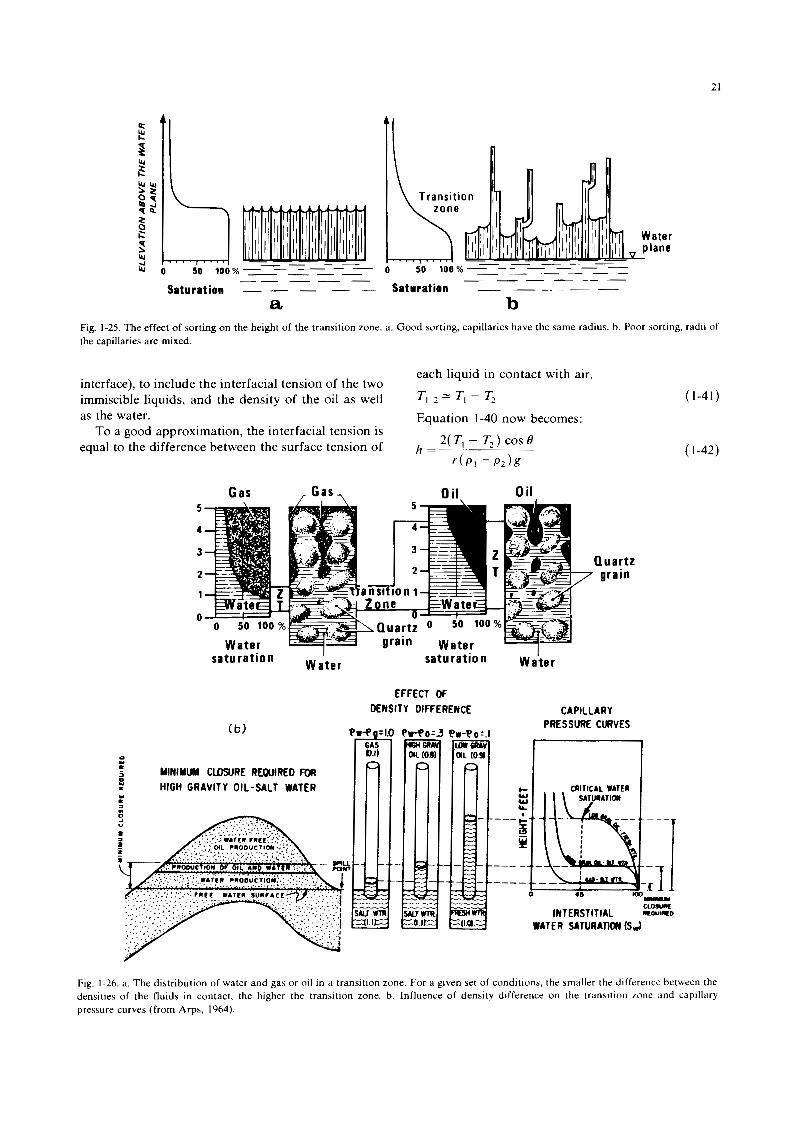
21
I 2 % I,,,.] g z s q R
ater E f lane
0 50 loo%----:-- - -_y UI 0 50 loo%--- - --- _ _ _ - UI
4
------ _- --- Saturation - - - - - Saturation - - - - __
a b Fig. 1-25. The effect of sorting on the height of the transition zone. a. Good sorting, capillaries have the same radius. b. Poor sorting, radii of the capillaries are mixed.
each liquid in contact with air.
T ~ - 2 = - T2
Equation 1-40 now becomes:
h =
interface), to include the interfacial tension of the two immiscible liquids, and the density of the oil as well as the water.
To a good approximation, the interfacial tension is equal to the difference between the surface tension of
(1-41)
2( TI - T2) cos 0 ( 1-42)
‘(PI - P*)g
Gas 0 il. 0 il
I saturation Wa\er Water sa t u rat ion
EFFECT OF DENSITY DIFFERENCE
Quartz * grain
CAPILLARY PRESSURE CURVES
Fig. 1-26. a. The distribution of water and gas or oil in a transition zone. For a given set of conditions, the smaller the difference between the densities of the fluids in contact, the higher the transition zone. b. Influence of density difference on the transition zone and capillary pressure curves (from Arps, 1964).
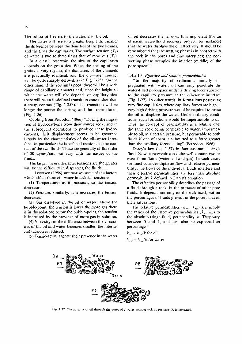
22
The subscript 1 refers to the water, 2 to the oil. The water will rise to a greater height the smaller
the difference between the densities of the two liquids, and the finer the capillaries. The surface tension ( T , ) of water is two to three times that of most oils (T2) .
In a clastic reservoir, the size of the capillaries depends on the grain-size. When the sorting of the grains is very regular, the diameters of the channels are practically identical, and the oil-water contact will be quite sharply defined, as in Fig. 1-25a. On the other hand, if the sorting is poor, there will be a wide range of capillary diameters and, since the height to which the water will rise depends on capillary size, there will be an ill-defined transition zone rather than a sharp contact (Fig. 1-25b). This transition will be longer the poorer the sorting, and the denser the oil (Fig. 1-26).
Quoting from Perrodon (1 966) “During the migra- tion of hydrocarbons from their source rock, and in the subsequent operations to produce these hydro- carbons, their displacement seems to be governed largely by the characteristics of the oil-water inter- face; in particular the interfacial tensions at the con- tact of the two fluids. These are generally of the order of 30 dynes/cm, but vary with the nature of the fluids.
The larger these interfacial tensions are the greater will be the difficulty in displacing the fluids. . . .
. . . Levorsen (1956) summarises some of the factors which affect these oil-water interfacial tensions:
(1) Temperature: as it increases, so the tension decreases.
(2) Pressure: similarly, as it increases, the tension decreases.
(3) Gas dissolved in the oil or water: above the bubble-point, the tension is lower the more gas there is in the solution; below the bubble-point, the tension is increased by the presence of more gas in solution.
(4) Viscosity: as the difference between the viscosi- ties of the oil and water becomes smaller, the interfa- cial tension is reduced.
(5) Tensio-active agents: their presence in the water
rain
or oil decreases the tension. It is important (for an efficient water-flood recovery project, for instance) that the water displays the oil effectively. It should be remembered that the wetting phase is in contact with the rock in the pores and fine interstices; the non- wetting phase occupies the interior (middle) of the pore-spaces”.
1.4.5.1.3. Effective and relative permeabilities “In the majority of sediments, initially im-
pregnated with water, oil can only penetrate the water-filled pore-space under a driving force superior to the capillary pressure at the oil-water interface (Fig. 1-27). In other words, in formations possessing very fine capillaries, where capillary forces are high, a very high driving pressure would be required to cause the oil to displace the water. Under ordinary condi- tions, such formations would be impermeable to oil. Thus the concept of permeability is a relative one; the same rock being permeable to water, impermea- ble to oil, at a certain pressure, but permeable to both fluids if one of them is submitted to a force greater than the capillary forces acting” (Perrodon, 1966).
Darcy’s law (eq. 1-37) in fact assumes a single fluid. Now, a reservoir can quite well contain two or even three fluids (water, oil and gas). In such cases, we must consider diphasic flow and relative permea- bility; the flows of the individual fluids interfere and their effective permeabilities are less than absolute permeability k defined in Darcy’s equation.
The effective permeability describes the passage of a fluid through a rock, in the presence of other pore fluids. It depends not only on the rock itself, but on the percentages of fluids present in the pores; that is, their saturations.
The relative permeabilities ( k , , , k, , , ) are simply the ratios of the effective permeabilities (k,.,, k , ) to the absolute (singe-fluid) permeability, k . They vary between 0 and 1, and can also be expressed as percentages : k , , = k , / k for oil k , , = k , / k for water
Fig. 1-27. The advance of oil through the pores of a water-bearing rock as pressure, P, is increased.
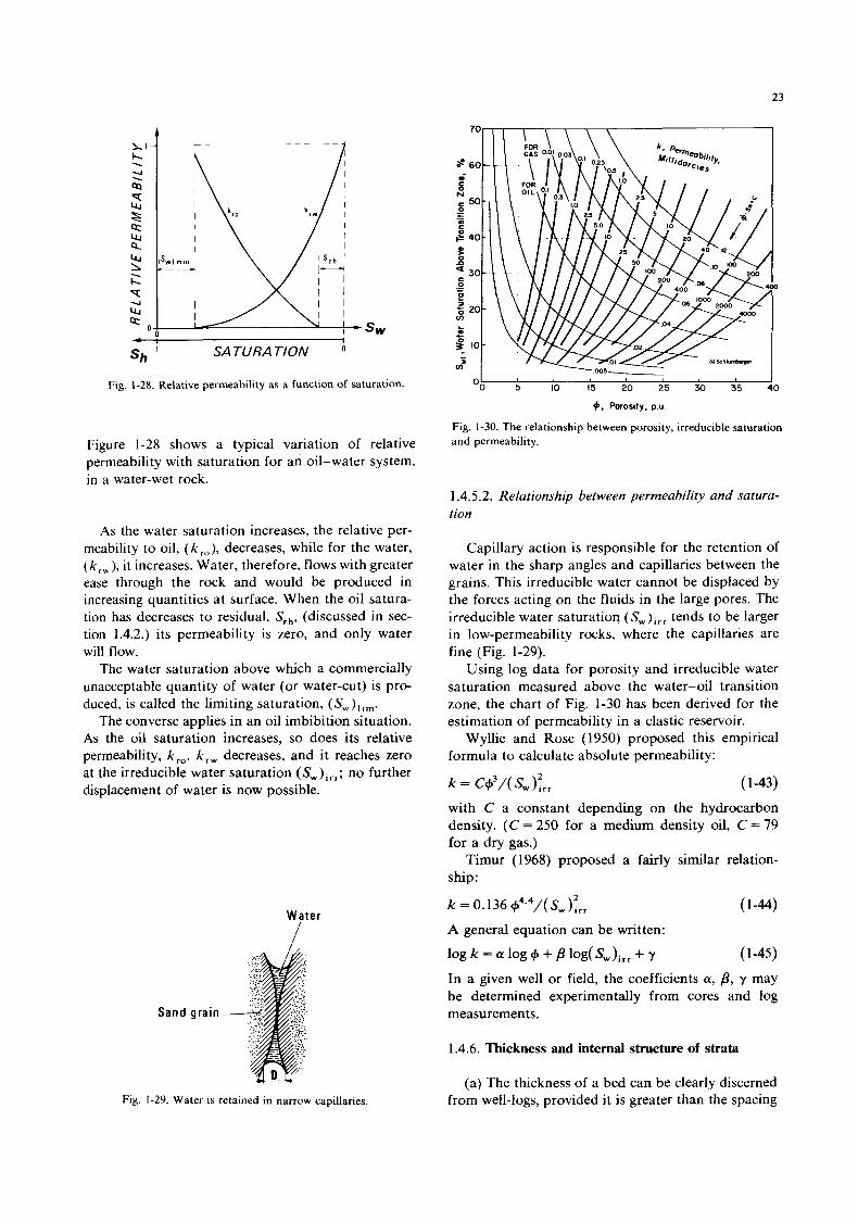
23
r ; I
SATURATION ' s h ' Fig. 1-28. Relative permeability as a function of saturation.
Figure 1-28 shows a typical variation of relative permeability with saturation for an oil-water system, in a water-wet rock.
As the water saturation increases, the relative per- meability to oil, ( k , , ) , decreases, while for the water, ( k , , ) , i t increases. Water, therefore, flows with greater ease through the rock and would be produced in increasing quantities at surface. When the oil satura- tion has decreases to residual, Srh, (discussed in sec- tion 1.4.2.) its permeability is zero, and only water will flow.
The water saturation above which a commercially unacceptable quantity of water (or water-cut) is pro- duced, is called the limiting saturation, ( S , ) , , m.
The converse applies in an oil imbibition situation. As the oil saturation increases, so does its relative permeability, kro. k , , decreases, and it reaches zero at the irreducible water saturation (Sw)irr; no further displacement of water is now possible.
W a t e r
I
Fig. 1-29. Water is retained in narrow capillaries.
+, Porosity. p.u.
Fig. 1-30. The relationship between porosity, irreducible saturation and permeability.
1.4.5.2. Relationship between permeability and suturu- tion
Capillary action is responsible for the retention of water in the sharp angles and capillaries between the grains. This irreducible water cannot be displaced by the forces acting on the fluids in the large pores. The irreducible water saturatioq ( Sw)irr tends to be larger in low-permeability rocks, where the capillaries are fine (Fig. 1-29).
Using log data for porosity and irreducible water saturation measured above the water-oil transition zone, the chart of Fig. 1-30 has been derived for the estimation of permeability in a clastic reservoir.
Wyllie and Rose (1950) proposed this empirical formula to calculate absolute permeability:
k = c+3/(sw);rr ( 1-43)
with C a constant depending on the hydrocarbon density. ( C = 250 for a medium density oil, C = 79 for a dry gas.)
Timur (1968) proposed a fairly similar relation- ship:
(1-44) 2 k = 0.136 +494/(Sw)i,,
A general equation can be written:
log k = a log + + p log(Sw)irr + y ( 1-45)
In a gven well or field, the coefficients a, B, y may be determined experimentally from cores and log measurements.
1.4.6. Thickness and internal structure of strata
(a) The thickness of a bed can be clearly discerned from well-logs, provided it is greater than the spacing
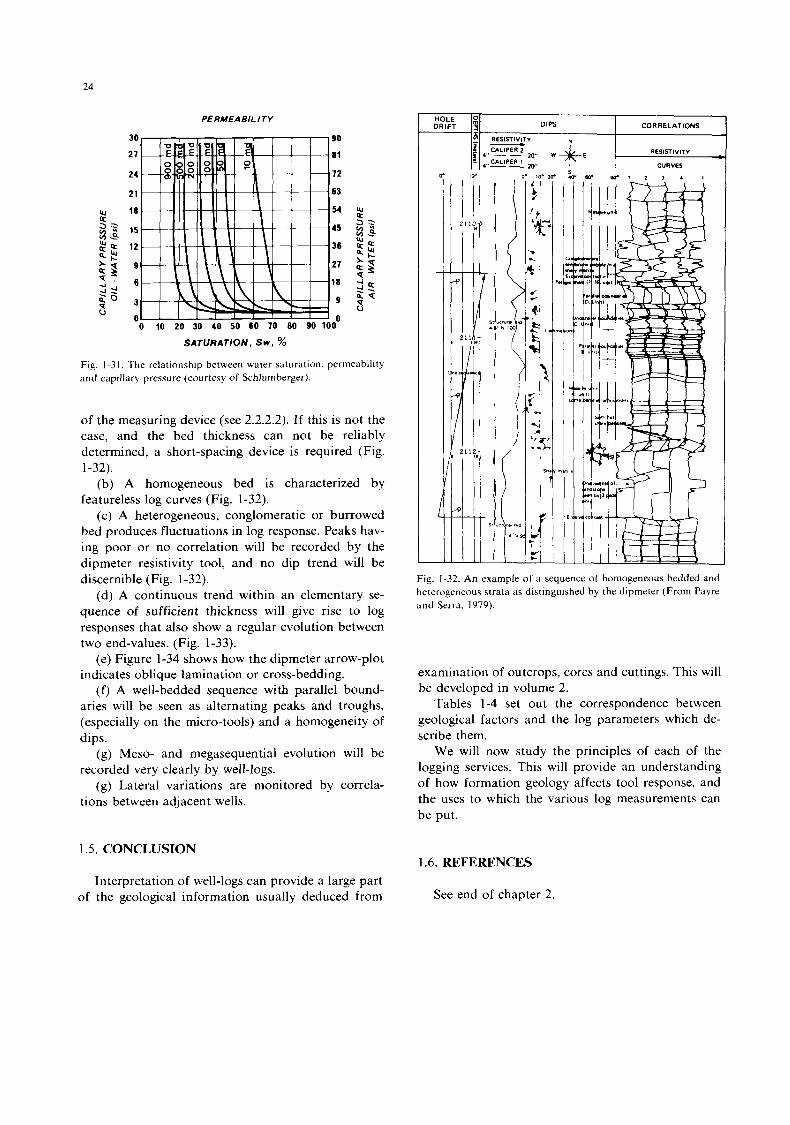
24
PERMEABILITY
SATURATION, S w , %
Fig. 1-3 I . The relationship between water saturation, permeability and capillary pressure (courtesy of Schlumberger).
of the measuring device (see 2.2.2.2). If this is not the case, and the bed thickness can not be reliably determined, a short-spacing device is required (Fig.
(b) A homogeneous bed is characterized by featureless log curves (Fig. 1-32).
(c) A heterogeneous, conglomeratic or burrowed bed produces fluctuations in log response. Peaks hav- ing poor or no correlation will be recorded by the dipmeter resistivity tool, and no dip trend will be discernible (Fig. 1-32).
(d) A continuous trend within an elementary se- quence of sufficient thickness will give rise to log responses that also show a regular evolution between two end-values. (Fig. 1-33).
(e) Figure 1-34 shows how the dipmeter arrow-plot indicates oblique lamination or cross-bedding.
(f) A well-bedded sequence with parallel bound- aries will be seen as alternating peaks and troughs, (especially on the micro-tools) and a homogeneity of dips.
(g) Meso- and megasequential evolution will be recorded very clearly by well-logs.
(g) Lateral variations are monitored by correla- tions between adjacent wells.
1-32).
1.5. CONCLUSION
Interpretation of well-logs can provide a large part of the geological information usually deduced from
DRIFT F
L
CORRELATIONS
RESlSTlVlTV
- ,CALIPER I m. CURVES
IP
1:
Fig. 1-32. An example of a sequence of homogeneous bedded and heterogeneous strata as distinguished by the dipmeter (From Payre and Serra, 1979).
examination of outcrops, cores and cuttings. This will be developed in volume 2.
Tables 1-4 set out the correspondence between geological factors and the log parameters which de- scribe them.
We will now study the principles of each of the logging services. This will provide an understanding of how formation geology affects tool response, and the uses to which the various log measurements can be put.
1.6. REFERENCES
See end of chapter 2.
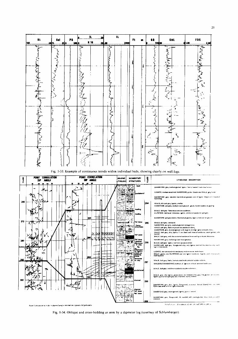
25
POINT DIP
n nao
F t )I
1
0 8 I CWL
Fig. 1-33. Example of continuous trends within individual beds, showing clearly on well-logs
FDC I
LITKXOGE DESCRIPTION
Fig. 1-34. Oblique and cross-bedding as seen by a dipmeter log (courtesy of Schlumberger)
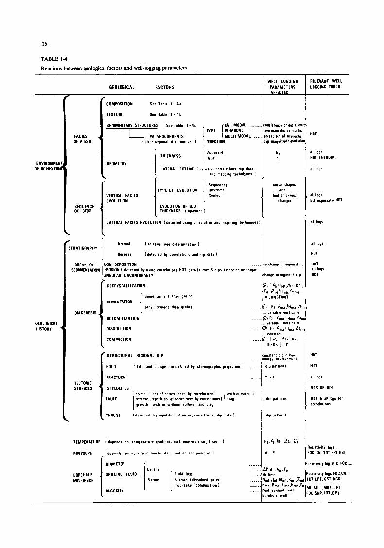
26
NON OEPOSlTlON ___._ ' EROSION I detected by using correlations.HOT data Icurves& dips ' ANGULAR UNCONFORMITY mapping technique 1
TABLE 1 - 4
Relations between geological factors and well-logging parameters
no change in regionaldip HOT
change in regional dip HOT a l l logs
I
RELEVANT WELL LOGGING TOOLS
W E L L LOGGING PARAMETERS AFFECTEO
GEOLOGICAL FACT0 R S
COMPOSITION See Table 1 - 4 a
TEXTURE See Table 1 - 4 b
SEDIMENTARY STRUCTURES See Table 1 - 4 c UNI -MODAL ....
TYPE El-MOOAL .
OlRECTlON MULTI-MOOAL . . . ! ' PALAEOCURRENTS
(af ter regional dip removal 1 pead cut of azmuths i p magnitude evolutmn
utsistency of dip azmut NO main dip azimuths 1 FACIES
OF A B E 0
al l logs HOT I GEOOIP I
all logs
Apparent [ true THICKNESS ha h t
ENVIRMIMEN OF MPOSlTKll
GEOLOGICAL HISTORY
GEOMETRY LATERAL EXTENT ( by uslng correlations,dip data
and mapping techniques 1
Sequences
Cycles TYPE OF EVOLUTION Rhythms I
EVOLUTION OF BE0 THICKNESS ( upwards
curve shapes and
bed thickness changes
VERTICAL FACIES EVOLUTION
all logs but especially HOT
SEOUENCE OF BEDS
LATERAL FACIES EVOLUTION I detected using correlation and mapping techniques 1 I all logs
Normal I relative age determmation 1
Reverse 1 detected by correlations and dip data ! STRATIGRAPHY a l l logs
HOT
BREAK OF SEDIMENTATION
0% [ 4'. ,At \ , R 3 I =CONSTANT
I , Pe. Pma ,IHma, Atma
RECRYSTALLIZATION
Same cement than grains
other cement than grains CEMENTATION
OOLOMlTlZATlON OIAGENESIS
OISSOLUTION
COMPACTION constant
( T i l t and plunge are defined by stereographic projection 1 dip patterns
STRUCTURAL REGIONAL OIP
FOLO
FRACTURE
STRESSES I STYLOLITES TECTONIC
HOT
H 01
all logs
NGS.GR.HO1
HOT & all logs lor correlations
dip patterns normal ( lack of series seen by correlations) w i t h or without reverse (repetition of series seen by correlations ) I drag growth wi th or without rollover and drag
I detected by repetition of series,correlations dip data 1 J dip patterns
Resistivity logs FOC,CNL,TOT.EPT,GST
Resistivity log, BHC. FOC ....
Resistivity logs, FOC.CNL.
i R f . P f . IHf , A t 1 .If
d i . P
9 m f . & l , I H m f , K m l , h 1 TOT. EPT. GST. NCS
d i . I& . pe di.hmc
TEMPERATURE I depends on temperature gradient. rock composit ion, f l o w 1
PRESSURE (depends on density of overburden, and on composit ion )
f DIAMETER
ORlLLlNG FLU10 Density
Fluid loss Filtrate I dissolved salts ) ..... mud -cake (composition 1
1 Nature [ RUGOSITV __._
BOREHOLE INFLUENCE
F0C.SNP. LOT.EPT 'ad contact w i t h lorehole wall
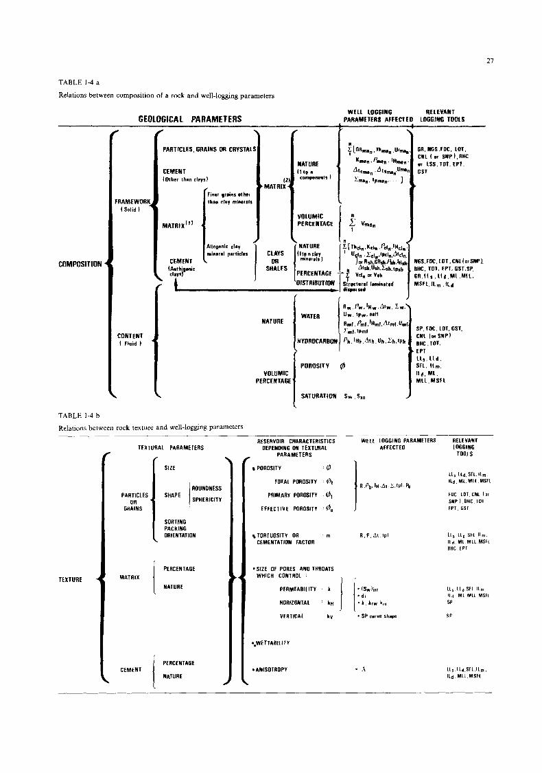
27
Finar grains other than clav minralr
MATRIX(^ J
TABLE 1-4 a
Relations between composition of a rock and well-loggng parameters
b MATRIX
WELL LOGGING RELEVANT 'ARAMETERS AFFECTED LOGGING TOOLS
Allogsnic clay mineral part ic lor
CEMENT ( Authignnie
GEOLOGICAL PARAMETERS
NATURE I l t o n campowants I
VOLUMIC PERCENTAGE
' NATURE f t to n c k y
minerals 1
PERCENTAGE
GR. NCS.fOC. LOT, CNL I or SNPI.BHC or LSS.TOT. EPT. G S T .
PARTICLES. GRAINS OR
CEMENT IOthsr thnn clays)
Finar grains other than clav minralr
Allogsnic clay mineral part ic lor I :RAMEWORI( . .
I Sol id I
CONTENT I Flu id I
b
MATRIX(^ J
CEMENT COMPOSITION
TABLE 1-4 b
( Authignnie clays)
A DIST RIBUTIOR
NATURE
VOLUMIC PERCENTAGE
POROSITY 8
SATURATION Sw , Sxo
Relations between rock texture and well-logging parameters WELL LOGGING PARAMETERS RELEVANT
AFFECTED LOGGING TOOLS
RESERVOIR CHARACTERISTICS DEPENDING ON TEXTURAL
PARAMETERS
POROSITY 8
TOTAL POROSITY 01
PRIMARY POROSITY 9,
EFFECTIVE POROSITY 0,
TEXTURAL PARAMETERS
\
SIZE
ROUNDNESS
'IiAPE SPHERICITY I PARTICLES OR
GRAINS
SORTING PACKING ORIENTATION TORTUOSITY OR rn
CEMENTATION FACTOR
'SIZE OF PORES AN0 THROATS WHICH CONTROL
PERMEABILITY h
HORIZONTAL hH
VERTICAL kv
PERCENTAGE
NATURE
MATRIX TEXTURE
- SP curve shape
WETTABILITY
PERCENTAGE
NATURE i CEMENT *ANISOTROPY
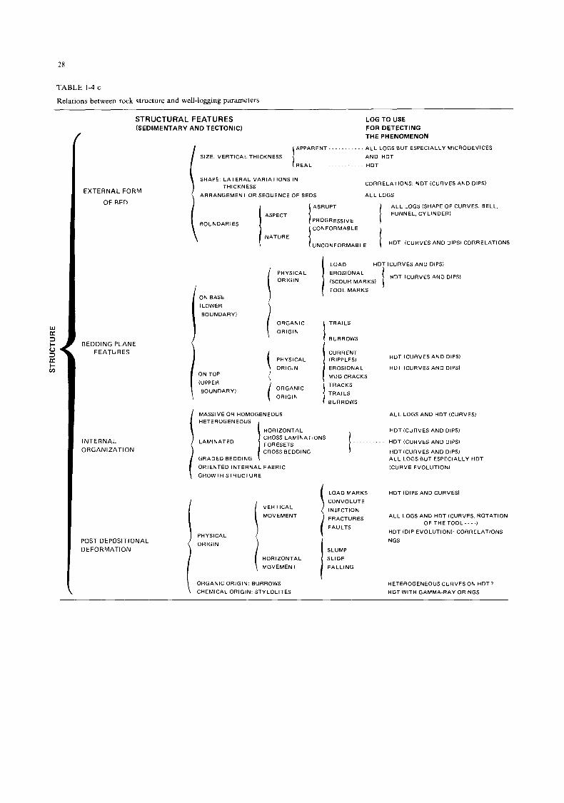
28
TABLE 1-4 c
Relations between rock structure and well-logging parameters
STRUCTURAL FEATURES (SEDIMEMTARY AND TECTONIC)
I
EXTERNAL FORM
OF BED
BEDDING PLANE FEATURES
INTERNAL 0 RGAN I ZATl ON
POST DEPOSITIONAL DEFORMATION
APPARENT . . . . . . . . . . .
1 REAL . . . . . . . . . . .
SIZE: VERTICAL THICKNESS
LOG TO USE FOR DETECTING THE PHENOMENON
A L L LOGS BUT ESPECIALLY MICRODEVICES
AND HDT
H DT
CORRELATIONS. NDT (CURVES AND DIPS)
A L L LOGS
SHAPE LATERAL VARIATIONS I N THICKNESS
ARRANGEMENT OR SEOUENCE OF BEDS
A L L LOGS (SHAPE OF CURVES BELL. FUNNEL, CYLINDER) I
I ABRUPT
PROGRESSIVE CONFORMABLE
HDT (CURVES AND DIPS) CORRELATIONS
1 I
ASPECT
BOUNDARIES
LOAD HDT (CURVES AND DIPS)
NATURE
ON BASE
(LOWER
BOUNDARY)
3N TOP
,UPPER
BOUNDARY)
PHYSICAL ORIGIN
ORGANIC
ORIGIN
PHYSICAL
ORIGIN
ORGANIC
ORIGIN
MASSIVE OR HOMOGENEOUS HETEROGENEOUS 1
HDT (CURVES AND DIPS) I EROSIONAL
(SCOUR MARKS)
TOOL MARKS ! TRAILS
BURROWS
CURRENT (RIPPLES)
EROSIONAL
MUD CRACKS
TRACKS
TRAILS I BURROWS
HORIZONTAL CROSS LAMINATIONS I FORESETS
LAMINATED
GRADED BEDDING
ORIENTED INTERNAL FABRIC
GROWTH STRUCTURE
PHYSICAL
ORIGIN
VERTICAL
MOVEMENT i HORIZONTAL
MOVEMENT
ORGANIC ORIGIN: BURROWS \ CHEMICAL ORIGIN: STYLOLITES
LOAD MARKS
CONVOLUTE
INJECTION
FRACTURES
FAULTS
HDT (CURVES AND DIPS)
HDT (CURVES AND DIPS)
A L L LOGS AND HDT (CURVES)
HDT (CURVES AND DIPS)
- HDT (CURVES AND DIPS)
HDT(CURVES AND DIPS) A L L LOGS BUT ESPECIALLY H D l
(CURVE EVOLUTION)
HDT (DIPS AND CURVES)
A L L LOGS AND HDT (CURVES. ROTATION
HOT (DIP EVOLUTION) CORRELATIONS
NGS
OF THE TOOL - - - -1
SLUMP
SLIDE
FALLING
HETEROGENEOUS CURVES ON HDT ?
HDT WITH GAMMA-RAY OR NGS
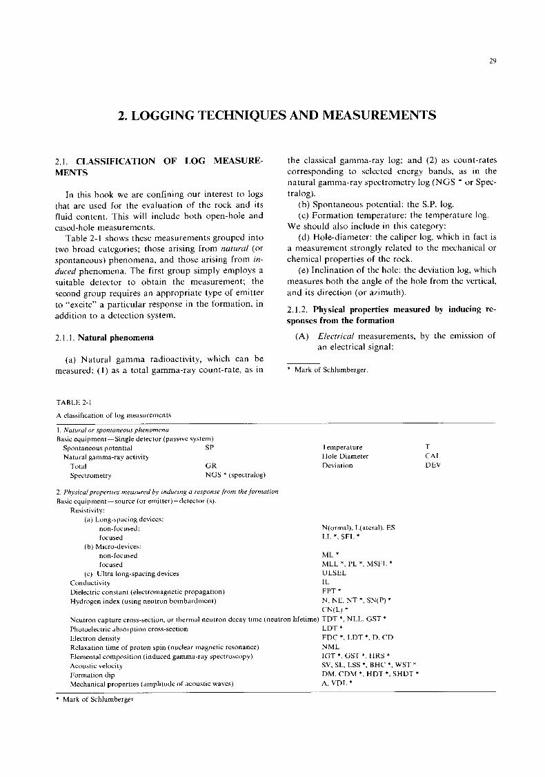
29
2. LOGGING TECHNIQUES AND MEASUREMENTS
2.1. CLASSIFICATION OF LOG MEASURE- MENTS
In this book we are confining our interest to logs that are used for the evaluation of the rock and its fluid content. This will include both open-hole and cased-hole measurements.
Table 2-1 shows these measurements grouped into two broad categories; those arising from natural (or spontaneous) phenomena, and those arising from in- duced phenomena. The first group simply employs a suitable detector to obtain the measurement; the second group requires an appropriate type of emitter to “excite” a particular response in the formation, in addition to a detection system.
2.1.1. Natural phenomena
(a) Natural gamma radioactivity, which can be measured: (1) as a total gamma-ray count-rate, as in
TABLE 2-1
A classification of log measurements
the classical gamma-ray log; and (2) as count-rates corresponding to selected energy bands, as in the natural gamma-ray spectrometry log (NGS * or Spec- tralog).
(b) Spontaneous potential: the S.P. log. (c) Formation temperature: the temperature log.
We should also include in this category: (d) Hole-diameter: the caliper log, which in fact is
a measurement strongly related to the mechanical or chemical properties of the rock.
( e ) Inclination of the hole: the deviation log, which measures both the angle of the hole from the vertical, and its direction (or azimuth).
2.1.2. Physical properties measured by inducing re- sponses from the formation
Elecfrical measurements, by the emission of an electrical signal:
(A)
* Mark of Schlumberger.
1 , Nuturul or sponruneous phenomenu Basic equipment-Single detector (passive system)
Spontaneous potential SP Natural gamma-ray activity
Total G R Spectrometry NGS * (spectralog)
Temperature Hole Diameter Deviation
2 . Physical properties measured by inducing u response from the formation Basic equipment - source (or emitter) + detector (s).
Resistivity: (a) Long-spacing devices:
non-focused: N(orma1). L(ateral), ES focused LL *, SFL *
(b) Micro-devices: non-focused ML * focused MLL *. PL *. MSFL *
ULSEL
EPT * N, NE. N T *. SN(P) * CN(L) *
(c) Ultra long-spacing devices Conductivity IL Dielectric constant (electromagnetic propagation) Hydrogen index (using neutron bombardment)
Neutron capture cross-section, or thermal neutron decay time (neutron lifetime) T D T *, NLL. GST * Photoelectric absorption cross-section Electron density Relaxation time of proton spin (nuclear magnetic resonance) Elemental composition (induced gamma-ray spectroscopy) Acoustic velocity Formation dip Mechanical properties (amplitude of acoustic waves)
LDT * FDC *, LDT *, D, C D NML IGT *, GST *. HRS * SV. SL, LSS *. BHC *. WST * DM. CDM *, HDT *, SHDT * A, VDL *
T CA L DEV
* Mark of Schlumberger
Resistivity or conductivity: (a) using an electrode system: electrical
survey (ES), laterolog (LL) *, micro- log (ML) *, microlaterolog (MLL) *, spherically focused log (SFL) *, mi- cro-spherically focused log (MSFL) *, high-resolution dipmeter (HDT) *, (SDT) *.
(b) using inductive coils: induction log (IL).
Dielectric constant, using inductive coils: electromagnetic propagat ion tool (EPT) *.
(B) Nuclear measurements, by the irradiation of formation with gamma rays or neutrons: Density. Gamma rays are emitted from a source. The Compton scattered gamma rays returning from the formation are detected: formation density or gamma- gamma log. (FDC *, D, CD, LDT *). Photo-electric absorption coefficient (re- lated to the mean Atomic Number). This is a low energy gamma-ray phenomenon and is measured in addition to density in the lithodensity log (LDT) *. The hydrogen index. The formation is continuously bombarded by high energy neutrons, which are slowed by successive elastic collisions with atomic nuclei, par- ticularly those of hydrogen. There are several techniques in use, in- volving the detection of: (a) Thermal neutrons, i.e. those neutrons
that have been slowed down to ther- mal energy: neutron-thermal neutron logging (CNL *, NT).
(b) Gamma rays emitted when these thermal neutrons are captured by atomic nuclei: neutron-gamma log- ging (N).
(c) Epithermal neutrons i.e. those neu- trons not yet slowed down to thermal energy: neutron-epithermal neutron logging NE, SNP *, CNL * (epithermal).
Macroscopic thermal neutron capture cross-section (Z). High-energy neutrons are emitted in short bursts. The rate of decay of the thermal neutron population in the formation is measured between bursts. This is a neutron capture phenom- enon: thermal neutron decay time (TDT) * or neutron lifetime logging (NLL).
* Mark of Schlumberger.
(5) Elemental composition. Gamma rays emitted from interactions between high energy neutrons and certain atomic nuclei are analyzed spectroscopically. There are three types of interaction important for induced gamma ray spectroscopy: (a) Fast neutron or inelastic interactions:
inelastic gamma ray spectrometry (IGT, GST), carbon-oxygen logging.
(b) Neutron capture: capture gamma ray spectrometry (GST, IGT), chlorine logging.
(c) Activation and subsequent decay of radio-isotopes: activation logging, high resolution spectrometry (HRS).
(6) Proton spin relaxation time. A pulsed DC magnetic field momentarily aligns the nuclear magnetic moments of the pro- tons. After the pulse, the time required for the protons of the formation to stop precessing about the Earth’s magnetic field is measured. This spin relaxation time can be used to evaluate residual oil. Nuclear magnetic resonance log (NML).
(C) Acoustic measurements-an acoustic signal is sent into the formation. We may measure: (1) The velocity of a compressional wave,
from the transit time between two re- ceivers: sonic log (SV, SL, BHC *). The shear-wave velocity can also be mea- sured.
( 2 ) The transit time from a surface gun to a downhole geophone: well seismic (WST) *.
(3) The amplitude of a selected peak or trough in the acoustic wave-train arriving at a receiver. The compressional or shear-wave arrivals may be of interest: amplitude logging (A).
(4) The relative amplitudes of the various components of the wave-train, the config- uration of the wave-train; variable den- sity logging (VDL) *, sonic waveform photography, well seismic (WST), bore- hole televiewer (BHTV).
2.2. PROBLEMS SPECIFIC TO WELL-LOG MEASUREMENTS
Although we would like logs to be direct measure- ments of the formation, log responses are invariably affected by the presence of the well-bore, certain near-hole phenomena associated with the drilling of the well, and the geometry of the logging tool itself. Operational problems may be posed by temperature and pressure in the well.
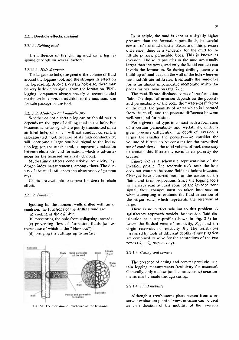
31
2.2.1. Borehole effects, invasion
2.2.1.1. Drilling mud
The influence of the drilling mud on a log re- sponse depends on several factors:
2.2.1.1.1. Hole diameter The larger the hole, the greater the volume of fluid
around the logging tool, and the stronger its effect on the log reading. Above a certain hole-size, there may be very little or no signal from the formation. Well- logging companies always specify a recommended maximum hole-size, in addition to the minimum size for safe passage of the tool.
2.2.1.1.2. Mud-type and mud-density Whether or not a certain log can or should be run
depends on the type of drilling mud in the hole. For instance, acoustic signals are poorly transmitted in an air-filled hole; oil or air will not conduct current; a salt-saturated mud, because of its high conductivity, will contribute a large borehole signal to the induc- tion log; (on the other hand, it improves conduction between electrodes and formation, which is advanta- geous for the focussed resistivity devices).
Mud-salinity affects conductivity, resistivity, hy- drogen index measurements, among others. The den- sity of the mud influences the absorption of gamma rays.
Charts are available to correct for these borehole effects
2.2.1.2. Invasion
Ignoring for the moment wells drilled with air or
(a) cooling of the drill-bit. (b) preventing the hole from collapsing inwards. (c) preventing flcw of formation fluids (an ex-
(d) bringing the cuttings up to surface.
emulsion, the functions of the drilling mud are:
treme case of which is the “blow-out”).
nola aais I Solid particular Grain o f the mud , (/Rmf) py Shale
kud-cake Porous and permaable
formation
Fig. 2-1. The formation of mud-cake on the hole-wall.
In principle, the mud is kept at a slightly higher pressure than the formation pore-fluids, by careful control of the mud-density. Because of this pressure difference, there is a tendency for the mud to in- filtrate porous, permeable beds. This is known as invasion. The solid particles in the mud are usually larger than the pores, and only the liquid content can invade the formation. So during drilling, there is a build-up of mud-cake on the wall of the hole wherever the mud-filtrate infiltrates. Eventually the mud-cake forms an almost impermeable membrane which im- pedes further invasion (Fig. 2-1).
The mud-filtrate displaces some of the formation fluid. The depth of invasion depends on the porosity and permeability of the rock, the “ water-loss’’ factor of the mud (the quantity of water which is liberated from the mud), and the pressure difference between well-bore and formation.
For a given mud-type, in contact with a formation of a certain permeability and wettability, under a given pressure differential, the depth of invasion is larger the smaller the porosity-we consider the volume of filtrate to be constant for the prescribed set of conditions- the total volume of rock necessary to contain this filtrate increases as its porosity de- creases.
Figure 2-2 is a schematic representation of the invasion profile. The reservoir rock near the hole does not contain the same fluids as before invasion. Changes have occurred both in the nature of the fluids and their proportions. Since the logging tools will always read at least some of the invaded zone signal, these changes must be taken into account when attempting to evaluate the fluid saturation of the virgin zone, which represents the reservoir at large.
There is no perfect solution to this problem. A satisfactory approach models the invasion fluid dis- tribution as a step-profile (shown in Fig. 2-3) be- tween the flushed zone of resistivity, R, , , and the virgin reservoir, of resistivity R , . The resistivities measured by tools of different depths of investigation are combined to solve for the saturations of the two zones (S, , , S, respectively).
2.2.1.3. Casing and cement
The presence of casing and cement precludes cer- tain logging measurements (resistivity for instance). Generally, only nuclear (and some acoustic) measure- ments can be made through casing.
2.2.1.4. Fluid mobility
Although a troublesome phenomenon from a re- servoir evaluation point of view, invasion can be used as an indication of the mobility of the reservoir
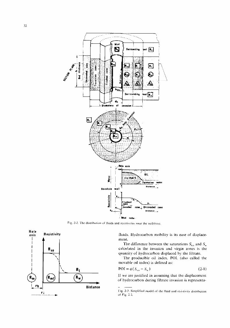
32
H o l e a x i s
I I I I I I I l
r-
L
i
Fig. 2-2. The
Resis t iv i ty
01.1."'.
;Mud cake
distribution of fluids and rrsistivltirs near the well-bore.
fluids. Hydrocarbon mobility is its ease of displace- ment.
The difference between the saturations S , , and S, calculated in the invasion and virgin zones is the quantity of hydrocarbon displaced by the filtrate.
The producible oil index, POI, (also called the movable oil index) is defined as:
POI = +( S,, - S,) (2-1 1 If we are justified in assuming that the displacement of hydrocarbon during filtrate invasion is representa- -~ ~~ Distance Fig. 2-3 . Simplified model o f the fluid and resis~ivity distribution o f Fig. 2-2.
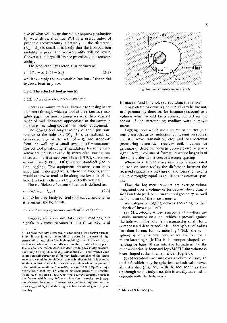
33
tive of what will occur during subsequent production by water-drive, then the POI is a useful index of probable recoverability. Certainly, if the difference (S,,, - S,) is small, it is likely that the hydrocarbon mobility is poor, and recoverability will be low *. Conversely, a large difference promises good recover- ability.
The recoverability factor, f, is defined as:
f = (S,,, - - S,) (2-2) which is simply the recoverable fraction of the initial hydrocarbons in place.
2.2.2. The effect of tool geometry
2.2.2.1. Tool diameter, excentralization
There is a minimum hole diameter (or casing inner diameter) through which a tool of a certain size may safely pass. For most logging services, there exists a range of tool diameters appropriate to the common hole-sizes, including special “ slim-hole’’ equipment.
The logging tool may take any of three positions relative to the hole axis (Fig. 2-4); centralized, ex- centralized against the wall (6 = O), and stood-off from the wall by a small amount (6 = constant). Correct tool positioning is mandatory for some mea- surements, and is ensured by mechanical means; one or several multi-armed centralizers (BHC); one-armed excentralizer (CNL, FDC); rubber stand-off (induc- tion logging). This equipment becomes even more important in deviated wells, where the logging sonde would otherwise tend to lie along the low side of the hole. (In fact, wells are rarely perfectly vertical.)
The coefficient of excentralization is defined as:
= 26/( d , - d,,,,, 1 (2-3) c is 1.0 for a perfectly centred tool sonde, and 0 when it is against the hole wall.
2.2.2.2. Spacing of sensors, depth of investigation
Logging tools do not take point readings, the signals they measure come from a finite volume of
* The fluid mobility is essentially a function of its relative permea- bility. If this is zero, the mobility is zero. In the case of high permeability (and therefore high mobility), the displaced hydro- carbon will often return rapidly once mud-circulation has stopped. If invasion is extremely deep, the deep-reading resistivity measure- ment may be very close to R,, rather than R , . The invaded zone saturation will appear to differ very little from that of the virgin zone. and we might conclude, erroneously, that mobility is poor. A similar conclusion could be drawn in a situation where the pressure differential is small, and invasion insignificant despite a high hydrocarbon mobility. (A zero or reversed pressure differential would have the same effect.) One should always carefully consider the factors which may influence invasion (porosity, rock-type, mud-density, formation pressure, etc) before computing satura- tions (S, , , and S,,,) and drawing conclusions about good or poor mobility.
Fig. 2-4. Sonde positioning in the hole.
formation (and borehole) surrounding the sensor. Single-detector devices (the S.P. electrode, the nat-
ural gamma-ray detector, for instance) respond to a volume whch would be a sphere, centred on the sensor, if the surrounding medium were homoge- neous.
Logging tools which use a source or emitter (cur- rent electrodes array, induction coils, neutron source, acoustic wave transmitter, etc) and one detector (measuring electrode, receiver coil, neutron or gamma-ray detector, acoustic receiver, etc) receive a signal from a volume of formation whose height is of the same order as the source-detector spacing.
Where two detectors are used (e.g. compensated neutron or sonic tools), the difference between the received signals is a measure of the formation over a distance roughly equal to the detector-detector spac- ing.
Thus the log measurements are average values, integrated over a volume of formation whose dimen- sions and shape depend on the tool geometry, as well as the nature of the measurement.
We categorize logging devices according to their “depth of investigation”:
(a) Micro-tools, whose sensors and emitters are usually mounted on a pad which is pressed against the hole-wall. The volume investigated is small; for a compensated density tool it is a hemisphere of radius less than 10 cm; for the microlog * (ML) the hemi- sphere is only a few centimetres radius; for a micro-laterolog * (MLL) it is trumpet shaped, ex- tending perhaps 10 cm into the formation; for the micro-spherically focussed log (MSFL) the volume is bean-shaped rather than spherical (Fig. 2-5).
(b) Macro-tools measure over a volume of, say, 0.5 to 5 m3, which may be spherical, cylindrical or even almost a disc (Fig. 2-5), with the tool sonde as axis. (Although not strictly true, this is usually assumed to coincide with the hole axis.)
* Mark of Schlumberger
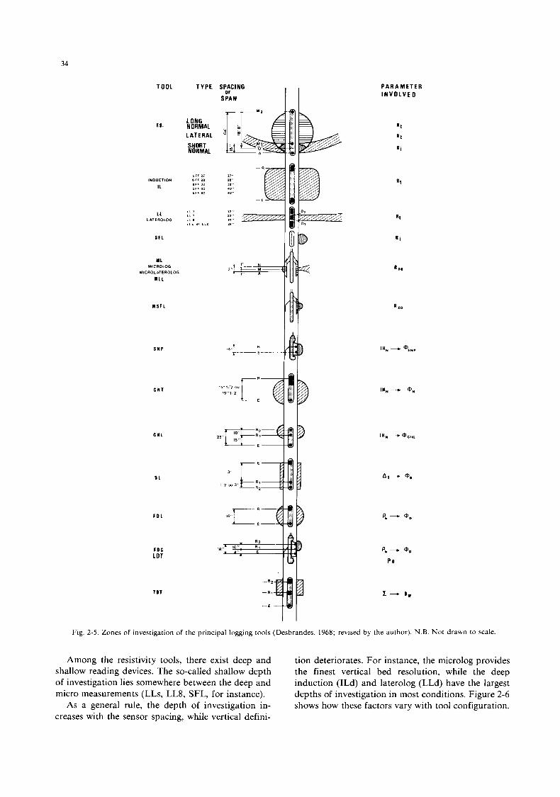
34
TOOL
ts.
INDUCTION
It
LL L 6TEROLOG
S F L
I t MICROLOG
UICROLATEROLOG
YLL
M S F L
S I P
G I 1
f D L
F D C LOT
I D 1
T Y P E SPACING or
S P A N I I
15 1 / 2 0"
1 9 1 2
E
25
P A R A M E T E R I N V O L V E D
R t
F - R 1
- E
Fig. 2-5. Zones of investigation of the principal logging tools (Desbrandes, 1968; revised by the author). N.B. Not drawn to scale.
Among the resistivity tools, there exist deep and shallow reading devices. The so-called shallow depth of investigation lies somewhere between the deep and micro measurements (LLs, LL8, SFL, for instance).
As a general rule, the depth of investigation in- creases with the sensor spacing, while vertical defini-
tion deteriorates. For instance, the microlog provides the finest vertical bed resolution, while the deep induction (ILd) and laterolog (LLd) have the largest depths of investigation in most conditions. Figure 2-6 shows how these factors vary with tool configuration.
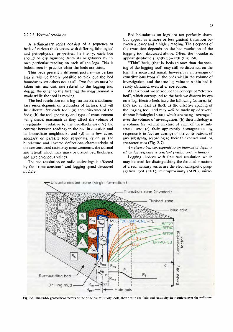
35
2.2.2.3. Vertical resolution
A sedimentary series consists of a sequence of beds of various thicknesses, with differing lithological and petrophysical properties. In theory, each bed should be distinguished from its neighbours by its own particular reading on each of the logs. This is indeed seen in practice when the beds are thck.
Thin beds present a different picture-on certain logs it will be barely possible to pick out the bed boundaries, on others not at all. Two factors must be taken into account, one related to the logging tool design, the other to the fact that the measurement is made while the tool is moving.
The bed resolution on a log run across a sedimen- tary series depends on a number of factors, and will be different for each tool: (a) the thickness of the beds; (b) the tool geometry and type of measurement being made, inasmuch as they affect the volume of investigation (relative to the bed-thickness); (c) the contrast between readings in the bed in question and its immediate neighbours; and (d) in a few cases, ancillary or parasite tool responses, (such as the blind-zone and inverse deflections characteristic of the conventional resistivity measurements, the normal and lateral) whch may mask or distort bed thickness, and give erroneous values.
The bed resolution on radio-active logs is affected by the “time constant” and logging speed discussed in 2.2.3.
Bed boundaries on logs are not perfectly sharp, but appear as a more or less gradual transition be- tween a lower and a higher reading. The steepness of the transition depends on the bed resolution of the logging tool, discussed above. Often, the boundaries appear displaced slightly upwards (Fig. 2-8).
“Thin” beds, (that is, beds thinner than the spac- ing of the logging tool) may still be discerned on the log. The measured signal, however, is an average of contributions from all the beds within the volume of investigation, and the true log value in a thin bed is rarely obtained, even after correction.
At this point we introduce the concept of “electro- bed”, which correspond to the beds we discern by eye on a log. Electro-beds have the following features: (a) they are at least as thick as the effective spacing of the logging tool, and may well be made up of several thinner lithological strata which are being “averaged” over the volume of investigation; (b) their lithology is a volume for volume mixture of each of these sub- strata; and (c) their apparently homogeneous log response is in fact an average of the contributions of any substrata, according to their thicknesses and log characteristics (Fig. 2-7).
An electro-bed corresponds to an interval of depth in which log response is constant (within certain limits).
Logging devices with fine bed resolution which may be used for distinguishng the detailed structure of a sedimentary series are the electromagnetic prop- agation tool (EPT), microproximity (MPL), micro-
Fig. 2-6. The radial geometrical factors of the principal resistivity tools, shown with the fluid and resistivity distributions near the well-bore.

36
INDUCTION
MICROLATEROLOG
$5 8 6 n a
COMPENSATED NEUTRON SONIC BHC
FORMATION DENSITY
Fig. 2-7. An example of a composite log, and “electrobed” zoning.
laterolog (MLL), or better still, the microlog (ML) and high-resolution dipmeters (HDT and SDT).
Since the electro-bed definition of the longer spac- ing tools is inferior to the micro-tools, it is customary to apply “depth-smoothing” or vertical averaging to the latter so as to render the bed resolution of all logs
Fig. 2-8. An example of “electrobeds”. The theoretical log re- sponse of a single-detector formation density tool (40 cm spacing), across a series of fine alternating beds of dolomite, anhydrite and salt. Note that the true density reading is not attained in beds significantly thinner than the tools spacing; and the upward dis- placement of the apparent bed boundaries.
more or less compatible, before an evaluation is at tempted.
2.2.3. Logging speed
Logging speeds are by no means the same for all types of log.
Since natural and induced radio-active phenomena are random by nature, it is necessary to accumulate count data over a period of time and compute the mean in order to obtain a representative reading. This accumulation or sampling period corresponds to the “Time constant” of conventional (capacitative- type) measuring equipment. The time constant is chosen according to the count-rate level and measure- ment precision desired; the logging speed is then usually adjusted such that the tool travels 1 f t (0.30 m) in one time constant period, as shown in Table 2-2. Vertical resolution of 2-3 f t (0.60-0.90 m) may be attained under these conditions.
Other factors which limit logging speed are galvanometer inertia (they must have sufficient time to deflect to the full value, which precludes very high logging speeds where high contrasts in readings are to be encountered), and various safety considerations, particularly cable tension and the risk of damage to pad-type equipment.
On log films, a speed marker provides a record of the logging speed. This is usually a small break or pip
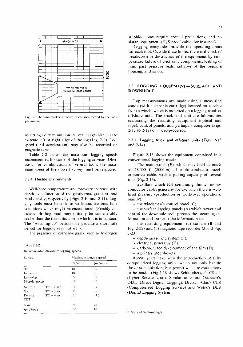
37
0 0 s
White intelval for recording speed control
Fig. 2-9. The time-marker, a record of distance moved by the cable per minute.
occurring every minute on the vertical grid-line at the extreme left or right edge of the log (Fig. 2-9). Tool speed (and acceleration) may also be recorded on magnetic tape.
Table 2-2 shows the maximum logging speeds recommended for some of the logging services. Obvi- ously, for combinations of several tools, the maxi- mum speed of the slowest survey must be respected.
2.2.4. Hostile environments
Well-bore temperature and pressure increase with depth as a function of the geothermal gradient, and mud density, respectively (Figs. 2-10 and 2-1 1). Log- ging tools must be able to withstand extreme hole conditions which might be encountered. (Freshly cir- culated drilling mud may initially be considerably cooler than the formations with which i t is in contact. The “warming-up” period may provide a short safe period for logging very hot wells.)
The presence of corrosive gases, such as hydrogen
TABLE 2-2
Recommended maximum logging speeds.
Survey Maximum logging speed
(ft/min) (m/min)
SP Induction La terolog Microlaterolog
Neutron GR Density TDT
Sonic Amplitude
TC = 2 sec TC = 3 sec TC = 4 sec
100 100 50 35
30 20 15
70 35
30 30 15 10
9 6 4.5
20 10
sulphide, may require special precautions, and re- sistant equipment (H,S-proof cable, for instance).
Logging companies provide the operating limits for each tool. Outside these limits, there is the risk of breakdown or destruction of the equipment by tem- perature failure of electronic components, leaking of mud past pressure seals, collapse of the pressure housing, and so on.
2.3. LOGGING EQUIPMENT-SURFACE AND DOWNHOLE
Log measurements are made using a measuring sonde (with electronic cartridge) lowered on a cable from a winch, which is mounted on a logging truck or offshore unit. The truck and unit are laboratories containing the recording equipment (optical and tape), control panels, and perhaps a computer (Figs. 2- 12 to 2- 18) or micro-processor.
2.3.1. Logging truck and offshore units (Figs. 2-13 and 2-14)
Figure 2-15 shows the equipment contained in a conventional logging truck:
- The main winch (E), which may hold as much as 26,000 f t (8000 m) of multi-conductor, steel- armoured cable, with a pulling capacity of several tons (Fig. 2-16).
- auxillary winch (G) containing thinner mono- conductor cable, generally for use when there is well- head pressure (production or work-over operations, mainly).
- the winchman’s control panel (C). - the surface logging panels (A) which power and
control the downhole tool, process the incoming in- formation and transmit the information to:
~ the recording equipment: (a) camera (B and Fig. 2-22) and (b) magnetic tape recorder (J and Fig. 2-23).
~ depth-measuring system (F). - electrical generator (H). - dark-room for development of the film (D). - a printer (not shown). Recent years have seen the introduction of fully
computerized logging units, which not only handle the data acquisition, but permit well-site evaluations to be made. (Fig.2-18 shows Schlumberger’s CSU * (Cyber Service Unit). Similar units are Gearhart’s DDL (Direct Digital Logging), Dresser Atlas’s CLS (Computerized Logging Service) and Welex’s DLS (Digital Logging System).
-~~ ~~
* Mark of Schlumberger
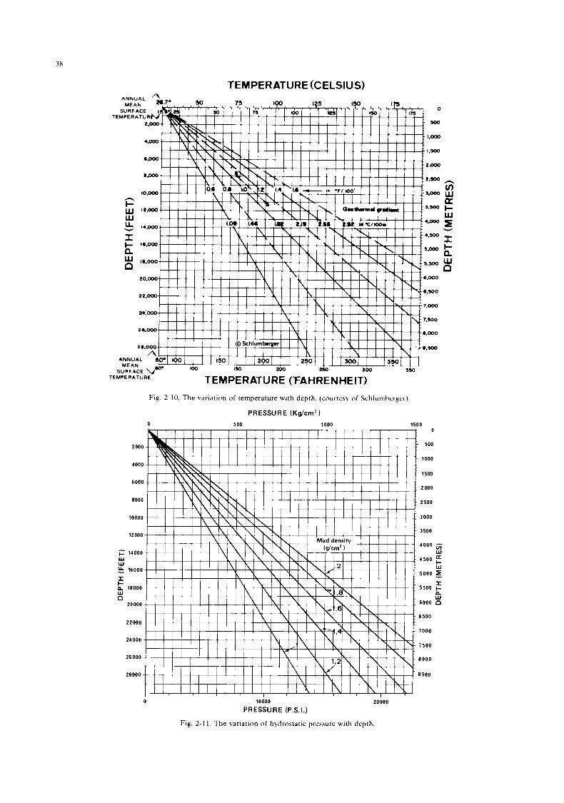
TE M PER AT UR E (% ELSI u S )
TEMPERATURE (FAHRENHEIT) TEMPERATURE
Fig 2-10 The variation of temperature with depth (Lourtesy o f Schlurnherger)
PRESSURE (Kg/cm2)
0 500 1000 1500
0 10000 20000
PRESSURE (P S I . )
Fig 2-1 1 The variation of hydrostdtiL preasure with depth
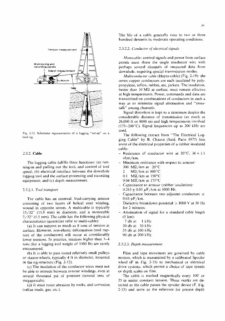
39
Tension measurement
Monitoring and recording panels
I I
Cable I
Fig. 2-12. Schematic representation of a logging “set-up” on a land-rig.
2.3.2. Cable
The logging cable fulfills three functions: (a) run- ning-in and pulling out the tool, and control of tool speed; (b) electrical interface between the downhole logging tool and the surface processing and recording equipment; and (c) depth measurement.
2.3.2.1. Tool trunsport
The cable has an external, load-carrying armour consisting of two layers of helical steel winding, wound in opposite senses. A multicable is typically 15/32” ( 1 1.8 mm) in diameter, and a monocable 7/32“ (5.5 mm). The cable has the following physical characteristics (quantities refer to multi-cable):
(a) I t can support as much as 8 tons of tension at surface. However, non-elastic deformation (and rup- ture of the conductors) will occur at considerably lower tensions. In practice, tensions higher than 3-4 tons (for a logging tool weight of 1500 lb) are rarely encountered.
(b) It is able to pass round relatively small pulleys or sheave-wheels, typically 4 ft in diameter, mounted in the rig-structure (Fig. 2-12).
(c) The insulation of the conductor wires must not be able to extrude between armour windings, even at several thousand psi of pressure (several tens of megapascals).
(d) I t must resist abrasion by rocks, and corrosion (saline muds, gas, etc.).
The life of a cable generally runs to two or three hundred descents in moderate operating conditions.
2.3.2.2. Conductor of electrical signuls
Monocable: control signals and power from surface panels must share the single conductor wire with perhaps several channels of measured data from downhole, requiring special transmission modes.
Multiconductor cable (Hepta-cable) (Fig. 2- 19): the seven copper conductors are each insulated by poly- propylene, teflon, rubber, etc, jackets. The insulation, better than 10 MQ at surface, must remain effective at high temperatures. Power, commands and data are transmitted on combinations of conductors in such a way as to minimize signal attenuation and “cross- talk” among channels.
Signal distortion is kept to a minimum despite the considerable distance of transmission (as much as 26,000 f t or 8000 m) and high temperatures involved (175-200°C). Signal frequencies up to 200 kHz are used.
The following extract from “The Electrical Log- ging Cable” by B. Chauve (Said, Paris 1977) lists some of the electrical properties of a rubber insulated cable:
Resistance of conductor wire at 20”C, 36 t- 1.5 ohm/km. Minimum resistance with respect to armour: 300 MQ/km at 20°C 2 MQ/kmat 100°C 0.1 MQ/kmat 150°C 0.04 MQ/km at 175°C Capacitance to armour (rubber insulation): 0.263 f 0.05 pF/km at 1000 Hz. Capacitance between two adjacent conductors ,< 0.03 pF/km. Dielectric breakdown potential >, 1000 V at 50 Hz for 2 minutes. Attenuation of signal for a standard cable length (5 km): 7 d b a t 1 kHz
30 db at 10 kHz 55 db at 100 kHz 90 db at 200 kHz
2.3.2.3. Depth measurement
Film and tape movement are governed by cable motion, which is transmitted by a calibrated Spooler wheel (F in Fig. 2-15) to mechanical or electrical drive systems, which permit a choice of tape speeds or depth scales on film.
The cable is marked magnetically every 100’ or 25 m under constant tension. These marks are de- tected as the cable passes the spooler device (F, Fig. 2-15) and serve as the reference for precise depth
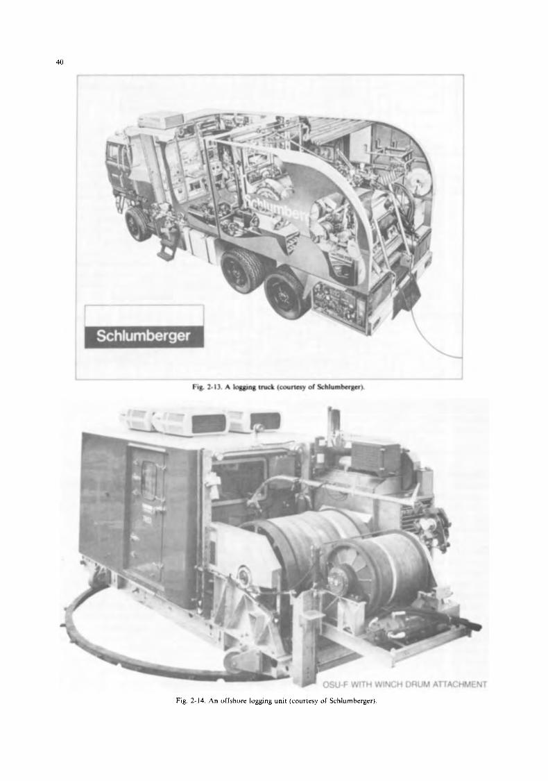
40
________ ___ -- ~- - - ~
Fig 2-13. A loggmg truck (courtesy of Schlumberger)
Fig. 2- 14. An offshore logging unit (courtesy of Schlumberger).
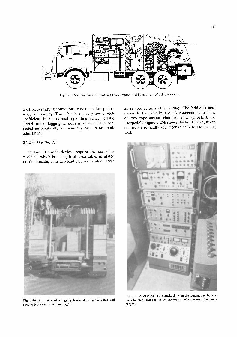
41
Fig 2-15 Sectional view of d logging truck (reproduced bv courte\y of Schlumberger)
control, permitting corrections to be made for spooler wheel inaccuracy. The cable has a very low stretch coefficient in its normal operating range; elastic stretch under logging tensions is small, and is cor- rected automatically, or manually by a hand-crank adjustment.
2.3.2.4. The “bridle”
Certain electrode devices require the use of a “bridle”, which is a length of deca-cable, insulated on the outside, with two lead electrodes which serve
:a.
Fig. 2-16. Rear view of a logging truck, showing the cable and spooler (courtesy of Schlumberger).
as remote returns (Fig. 2-20a). The bridle is con- nected to the cable by a quick-connection consisting of two rope-sockets clamped in a split-shell, the “torpedo”. Figure 2-20b shows the bridle head, which connects electrically and mechanically to the logging tool.
Fig. 2-17. A view inside the truck. showing the logging panels, tape recorder (top) and part of the camera (right) (courtesy of Schlum- berger).
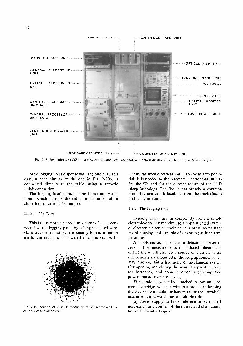
42
MAGNETIC TAPE UNIT
GENERAL ELECTRONIC UNIT
OPTICAL ELECTRONICS UNIT
CENTRAL PROCESSOR UNIT No.1
CENTRAL PROCESSOR UNIT No. 2
V E N TIL AT ION BLOWER UNIT
N U M E R I C A L DISPLAY CARTRIDGE TAPE UNIT
OPTICAL FILM UNIT
TOOL INTERFACE UNIT
TOOL MODULES
DEPTH C O N T R O L
OPTICAL MONITOR UNIT
TOOL POWER UNIT
KEYBOARD / PRINTER UNIT COMPUTER AUXILIARY UNIT
Fig. 2-18 Schlumberger’s CSU’ -a view of the computers. tdpe unit4 dnd opticdl di\play 4eCtlon (courte4y o f Schluniberger)
Most logging tools dispense with the bridle. In this case, a head similar to the one in Fig. 2-20b, is connected directly to the cable, using a torpedo quick-connection.
The logging head contains the important weak- point, which permits the cable to be pulled off a stuck tool prior to a fishing job.
ciently far from electrical sources to be at zero poten- tial. I t is needed as the reference electrode-at-infinity for the SP, and for the current return of the LLD (deep laterolog). The fish is not strictly a common ground return, and is insulated from the truck chassis and cable armour.
2.3.3. The logging tool 2.3.2.5. The “fish”
This is a remote electrode made out of lead, con- nected to the logging panel by a long insulated wire, via a truck installation. It is usually buried in damp earth, the mud-pit, or lowered into the sea, suffi-
Fig. 2-19. Section of a multi-conductor cable (reproduced by courtesy of Schlumberger).
Logging tools vary in complexity from a simple electrode-carrying mandrel, to a sophisticated system of electronic circuits, enclosed in a pressure-resistant metal housing and capable of operating at high tem- peratures.
All tools consist at least of a detector, receiver or sensor. For measurements of induced phenomena (2.1.2) there will also be a source or emitter. These components are mounted in the logging sonde, which may also contain a hydraulic or mechanical system (for opening and closing the arms of a pad-type tool, for instance), and some electronics (preamplifier, power-transformer Fig. 2-2 1 a).
The sonde is generally attached below an elec- tronic cartridge, which carries in a protective housing the electronic modules or hardware for the downhole instrument, and which has a multiple role:
(a) Power supply to the sonde emitter system ( i f necessary), and control of the timing and characteris- tics of the emitted signal.
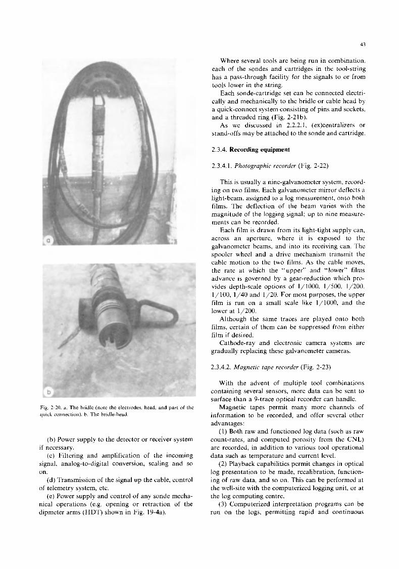
43
Fig. 2-20. a. The bridle (note the electrodes, head, and part of the quick connection). b. The bridle-head.
(b) Power supply to the detector or receiver system i f necessary.
(c) Filtering and amplification of the incoming signal, analog-to-digital conversion, scaling and so on.
(d) Transmission of the signal up the cable, control of telemetry system, etc.
(e) Power supply and control of any sonde mecha- nical operations (e.g. opening or retraction of the dipmeter arms (HDT) shown in Fig. 19-4a).
Where several tools are being run in combination, each of the sondes and cartridges in the tool-string has a pass-through facility for the signals to or from tools lower in the string.
Each sonde-cartridge set can be connected electri- cally and mechanically to the bridle or cable head by a quick-connect system consisting of pins and sockets, and a threaded ring (Fig. 2-21b).
As we discussed in 2.2.2.1, (ex)centralizers or stand-offs may be attached to the sonde and cartridge.
2.3.4. Recording equipment
2.3.4.1. Photographic recorder (Fig. 2-22)
This is usually a nine-galvanometer system, record- ing on two films. Each galvanometer mirror deflects a light-beam, assigned to a log measurement, onto both films. The deflection of the beam varies with the magnitude of the logging signal; up to nine measure- ments can be recorded.
Each film is drawn from its light-tight supply can. across an aperture, where i t is exposed to the galvanometer beams, and into its receiving can. The spooler wheel and a drive mechanism transmit the cable motion to the two films. As the cable moves, the rate at which the “upper” and “lower” films advance is governed by a gear-reduction which pro- vides depth-scale options of I / l O O O , 1/500, 1/200. 1/100, 1/40 and 1/20. For most purposes, the upper film is run on a small scale like 1/1000, and the lower at 1/200.
Although the same traces are played onto both films, certain of them can be suppressed from either film if desired.
Cathode-ray and electronic camera systems are gradually replacing these galvanometer cameras.
2.3.4.2. Magnetic tape recorder (Fig. 2-23)
With the advent of multiple tool combinations containing several sensors, more data can be sent to surface than a 9-trace optical recorder can handle.
Magnetic tapes permit many more channels of information to be recorded, and offer several other advantages :
( 1 ) Both raw and functioned log data (such as raw count-rates, and computed porosity from the CNL) are recorded, in addition to various tool operational data such as temperature and current level.
(2) Playback capabilities permit changes in optical log presentation to be made, recalibration, function- ing of raw data, and so on. This can be performed at the well-site with the computerized logging unit, or at the log computing centre.
(3) Computerized interpretation programs can be run on the logs, permitting rapid and continuous
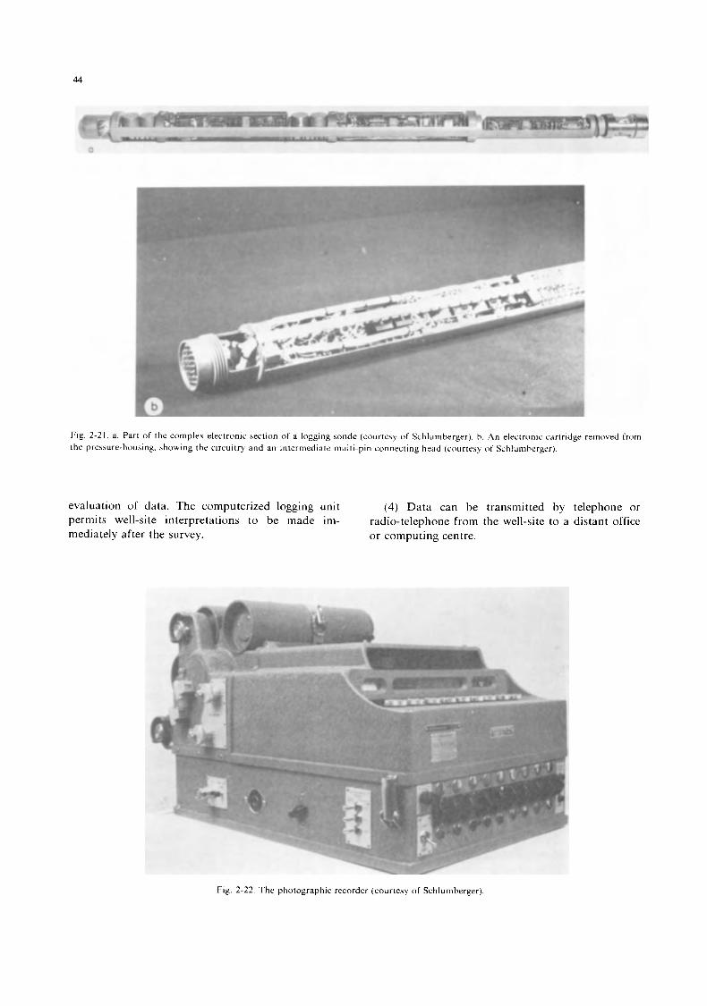
44
Fig. 2-21. a. Part of the complex electronic section of a logging sonde (courtesy of Schlumberger). h . An electronic cartridge reinoved from the pressure-housing, showing the circuitry and an intermediate multi-pin connecting head (courtesy of Schlunihergcr).
evaluation of data. The computerized logging unit (4) Data can be transmitted by telephone or permits well-site interpretations to be made im- radio-telephone from the well-site to a distant office mediately after the survey. or computing centre.
Fig. 2-22. The photographic recorder (courtesy of Schlumherger)
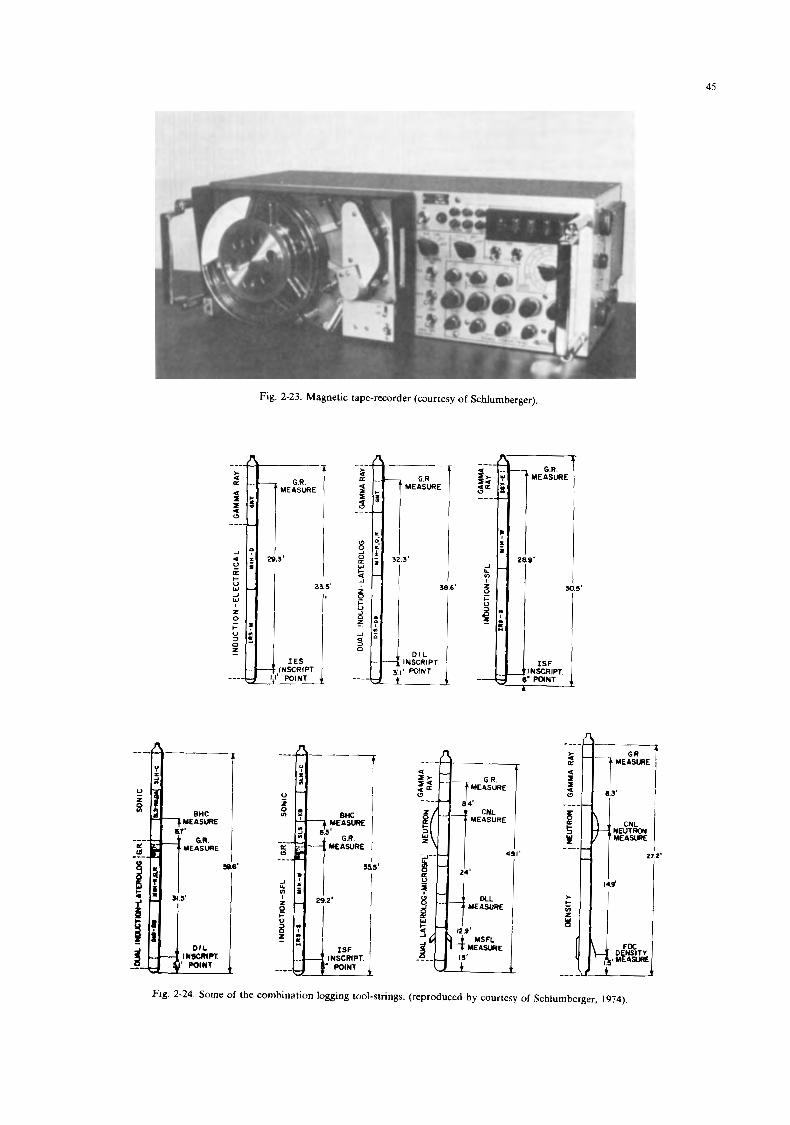
45
Fig. 2-23. Magnetic tape-recorder (courtesy of Schlumberger).
"
Fig. 2-24. Some of the combination logging tool-strings. (reproduced by courtesy of Schlumberger, 1974)
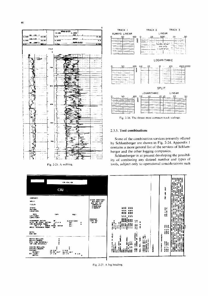
46
I
Fig. 2-25. A well-log.
OTHER SCRVICCS- nLL-ntrL-tP
BUC HDT E l l COMPPSlTE CYBLRLPOK CVBCRDIP
TRACK I TRACK 2 TRACK 3
ALWAYS LINEAR LINEAR
LOGARl THMlC
0 0 000
t x
SPLIT LOGARITHMIC LINEAR
Fig. 2-26. The threee most common track scalings
2.3.5. Tool combinations
Some of the combination services presently offered by Schlumberger are shown in Fig. 2-24. Appendix 1 contains a more general list of the services of Schlum- berger and the other logging companies.
Schlumberger is at present developing the possibil- ity of combining any desired number and types of tools, subject only to operational considerations such
l.l Y
P I
- Fig. 2-27. A log heading.
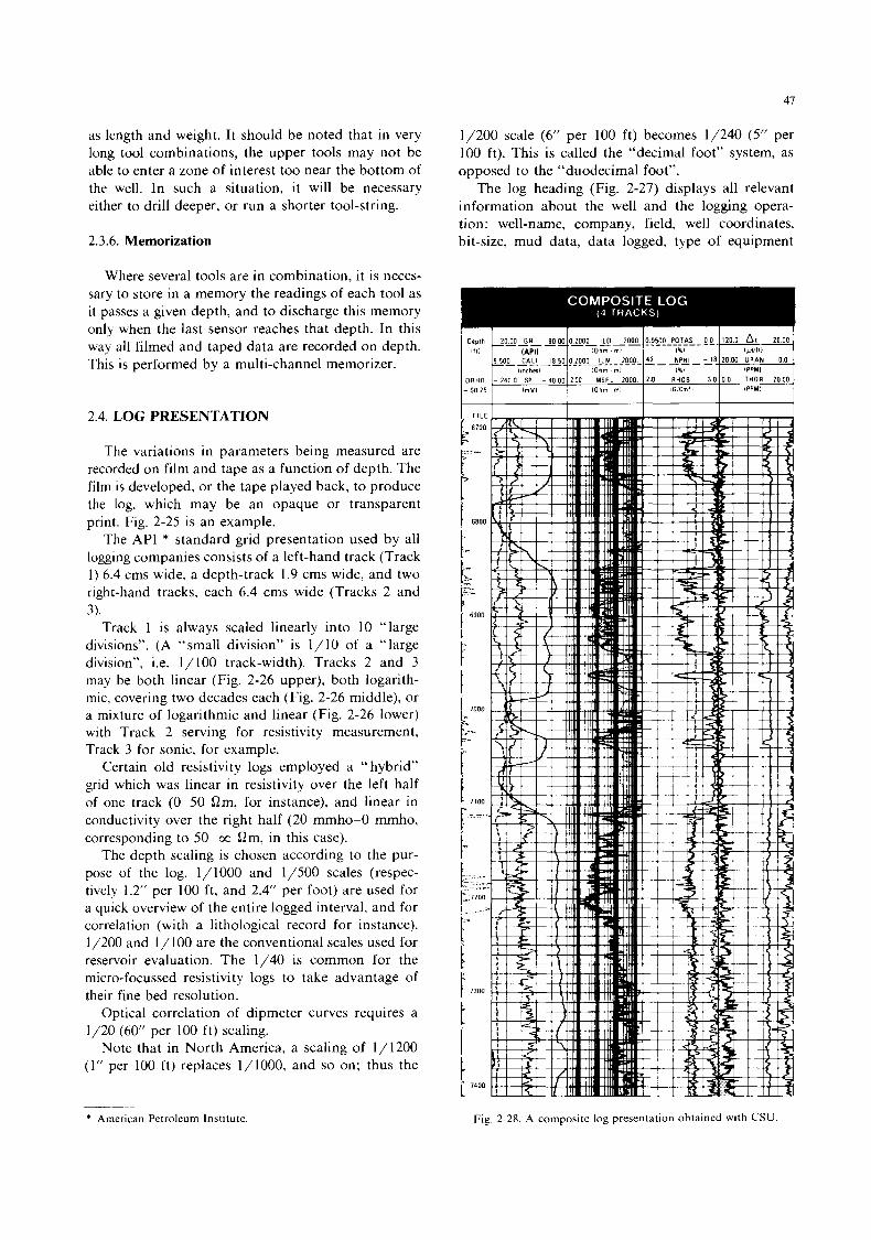
47
as length and weight. It should be noted that in very long tool combinations, the upper tools may not be able to enter a zone of interest too near the bottom of the well. In such a situation, it will be necessary either to drill deeper, or run a shorter tool-string.
2.3.6. Memorization
Where several tools are in combination, it is neces- sary to store in a memory the readings of each tool as it passes a given depth, and to discharge this memory only when the last sensor reaches that depth. In this way all filmed and taped data are recorded on depth. This is performed by a multi-channel memorizer.
2.4. LOG PRESENTATION
The variations in parameters being measured are recorded on film and tape as a function of depth. The film is developed, or the tape played back, to produce the log, which may be an opaque or transparent print. Fig. 2-25 is an example.
The API * standard grid presentation used by all logging companies consists of a left-hand track (Track 1 ) 6.4 crns wide, a depth-track 1.9 crns wide, and two right-hand tracks, each 6.4 crns wide (Tracks 2 and 3).
Track 1 is always scaled linearly into 10 “large divisions”. (A “small division” is 1/10 of a “large division”, i.e. 1/100 track-width). Tracks 2 and 3 may be both linear (Fig. 2-26 upper), both logarith- mic, covering two decades each (Fig. 2-26 middle), or a mixture of logarithmic and linear (Fig. 2-26 lower) with Track 2 serving for resistivity measurement, Track 3 for sonic, for example.
Certain old resistivity logs employed a “hybrid” grid which was linear in resistivity over the left half of one track (0-50 Qm, for instance), and linear in conductivity over the right half (20 mmho-0 mmho, corresponding to 50-00 Qm, in this case).
The depth scaling is chosen according to the pur- pose of the log. 1/1000 and 1/500 scales (respec- tively 1.2” per 100 ft, and 2.4“ per foot) are used for a quick overview of the entire logged interval, and for correlation (with a lithological record for instance). 1 /200 and 1 / 100 are the conventional scales used for reservoir evaluation. The 1/40 is common for the micro-focussed resistivity logs to take advantage of their fine bed resolution.
Optical correlation of dipmeter curves requires a 1/20 (60” per 100 f t ) scaling.
Note that in North America, a scaling of 1/1200 ( I ” per 100 ft) replaces 1/1000, and so on; thus the
1/200 scale (6” per 100 ft) becomes 1/240 (5” per 100 ft). This is called the “decimal foot” system, as opposed to the “duodecimal foot”.
The log heading (Fig. 2-27) displays all relevant information about the well and the logging opera- tion: well-name, company, field, well coordinates, bit-size, mud data, data logged, type of equipment
e
* American Petroleum Institute. Fig. 2-28. A composite log presentation obtained with CSU.
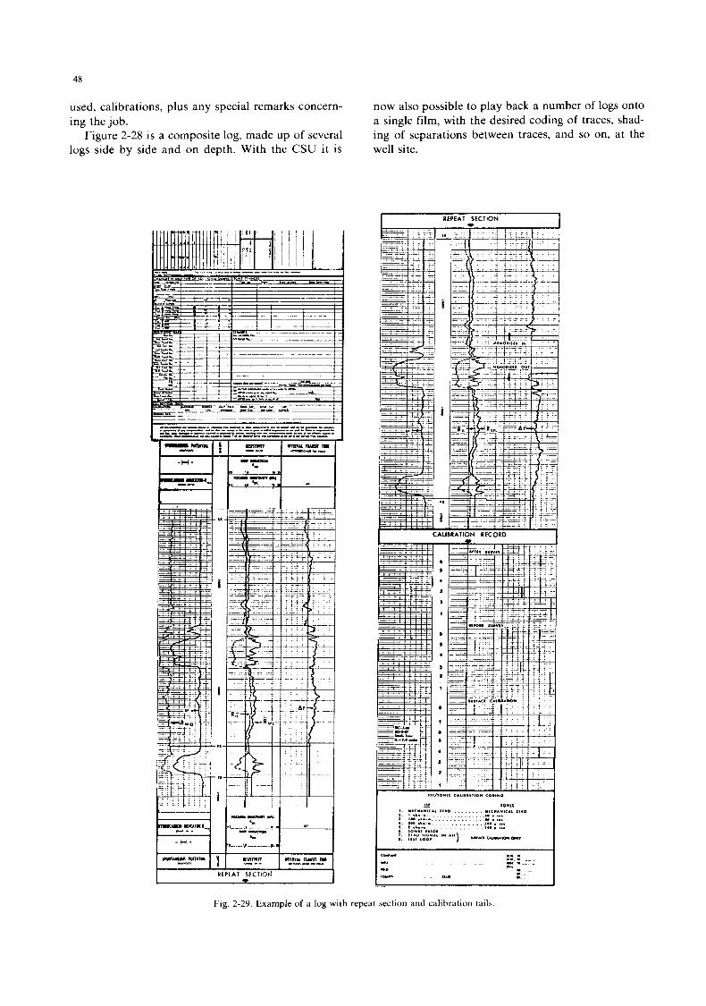
48
used, calibrations, plus any special remarks concern- ing the job.
Figure 2-28 is a composite log, made up of several logs side by side and on depth. With the CSU it is
1
1 1 I 1 1 1
I YEPLAT SECTION * 1
now also possible to play back a number of logs onto a single film, with the desired coding of traces, shad- ing of separations between traces, and so on, at the well site.
I REPEAT SECTION 1
- 1 1 1 W!u I. "#<*.*1C1, 11.0 .... . .. . . "lC".*,C.L z1.0 1 . I.).-.. .......__._._.. a,.... I . 0.. ...-.. . . . . . . _ _ _ _ _ .... . ... a . *.* ....I. . . . . . . . . . . ... I.. ~ ... s. I .L.-. . . . . . . . . . . I.. . ... 6 . ,o*m 1,101 I . 2 1 . 0 %or*., I" .I, ,. llllLool ) -*---l*-v
Fig. 2-29. Example of a log with repeat section and calibration tails.
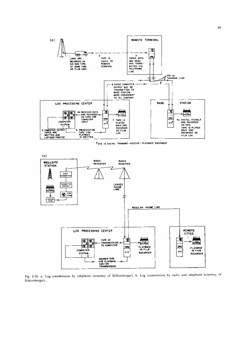
49
(a )
RECORDED ON DIG. MAG TAPE AT SAME TIME AS FILM LOOS
it _ - 2
TAPE I S TAKEN TO REMOTE TERMINAL
REMOTE TERMINAL
AN0 TRANS- MITTED VIA TELEPHONE
I LINE I I
4 b RECEIVED DATA ARE RECORDED
*DTE IS DIGITAL TRANSMIT-RECEIVE -PLAYBACK EWIPMENT
RADIO RADIO RECEIVER
LEASED PHONE LINE 1
I A 1 REGULAR PHONE LINE
I I
LOG PROCESSING CENTER
TAPE OF TRANSMISSION TO COMPUTER
ANSWERTAPE L-r' FOR PLAYBACK d AND/ OR TRANSMISSION
REMOTE CITIES gzK RECORDER
Fig. 2-30. a. Log transmission by telephone (courtesy of Schlumberger). b. Log transmission by radio and telephone (courtesy of
Schlumberger).
50
2.5. REPEATABILITY AND CALIBRATIONS (see Appendix 5 for more details)
At the end of a log, a repeat section and calibra- tion tail are usually attached (Fig. 2-29, right). The repeat section verifies that the tool is functioning consistently. For radio-active logs, several repeat sec- tions may be run for subsequent stacking (averaging) to reduce statistical variations (e.g. NGS and TDT).
A calibration record is made on film and tape before and after the survey, to show that the equip- ment was correctly adjusted, and that no drift in adjustment has occurred during the log. For certain tools, a “master calibration” is made at the workshop prior to the logging operation, using laboratory equipment. The well-site calibration repeats this ad- justment using portable calibration ‘‘jigs’’ (FDC, CNL, GR. . . Appendix 5) . Other tools have their own internal calibrators (IL, LL, ...), and may be ad- justed while down-hole.
2.6. DATA TRANSMISSION
Taped data can be transmitted by telephone, or radio and telephone (Fig. 2-30) to a log computing centre or company office if quick decisions, or rapid interpretation, are to be made away from the well-site.
2.7. REFERENCES
Allaud, L. and Martin, M., 1976. Schlumberger: Histoire d’une
Arps, J.J., 1964. Engineering concepts useful in oil finding. Bull.
Chilingar. G.V., 1969. Deltaic and Shallow Marine Deposits.
Chombart, L.G., 1959. Reconnaissance et evaluation des forma-
Technique. Berger-Levrault, Pans.
Am. Assoc. Pet. Geol., vol. 48 (2).
L.M.J.U. van Straaten, ed., Elsevier, Amsterdam.
tions par diagraphies electriques et nucleaires. Technip, Paris.
Choquette, P.W. and Pray, L.C., 1970. Geologic nomenclature and classification of porosity in sedimentary carbonates. Bull. Am. Assoc. Pet. Geol., 54 (2).
Clavier, C., Coates, G. and Dumanoir, J., 1977. The theoretical and experimental basis for the “dual water” model for the interpretation of shaly sands. Soc. Pet. Eng.. AIME. Pap. No. 6859.
Dadone, R., 1958. Diagraphies differees. Tome 1 des “Techniques d’exploration profonde dans la recherche du petrole”. Technip. Pans.
Desbrandes, R., 1968. Theorie et interpretation des diagraphies. Technip, Paris.
De Witte, L., 1950. Relations between resistivities and fluid con- tents of porous rocks. Oil Gas J.. August 24.
Flandrin, J. and Chapelle, J., 1961. Le petrole. Technip. Paris. Guillemot, J., 1964. Cours de Geologie du Petrole. Technip, Paris. Guyod, H., 1952. Electrical Well Logging. Fundamentals, Hous-
ton. Guyod, H., 1969. Geophysical Well Logging. Guyod, Houston. Lynch, E.J., 1962. Formation Evaluation. Harper & Row. New
York. Martin, M., 1957. Possibilites actuelles des methodes de diagra-
phies electriques et nucleaires. Technip, Paris. Millot, G., 1969. Geologie des argiles. Masson, Paris. Patchett, J.G., 1975. An investigation of shale conductivity.
SPWLA, 16th Am. Log. Symp. Trans., paper V . Perrodon, A., 1966. Geologie du petrole. Presses Univ. Franq..
Paris. Pirson, S.J., 1963. Handbook of Well Log Analysis for Oil and
Gas, Formation Evaluation. Prentice Hall, New York. Schlumberger, 1959. Etudes des sondages par les methodes
Schlumberger, document 8. Log interpretation: Vol. I. Princi- ples 1972; Vol. 11. Applications 1974; Charts 1979. Soc. Pet. Eng. AIME, 1958. Petroleum Transactions, vol. I: Well log- ging.
Timur, A,, 1968. An investigation of permeability. porosity and residual water saturation relationship for sandstone reservoirs. Log Analyst, 9 (4).
Waxrnan, M.H. and Smits, L.J.M., 1968. Electrical conductivities in oil-bearing shaly sands. J. Soc. Pet. Eng.. 8 (2).
Wyllie, M.R.J., 1957. The Fundamentals of Electric Log Interpre- tation. Academic Press, New York.
Wyllie, M.R.J. and Rose, W.D.. 1950. Some theoretical considera- tions related to the quantitative evaluation of the physical characteristics of reservoir rock from electrical log data. J. Pet. Technol., 189.
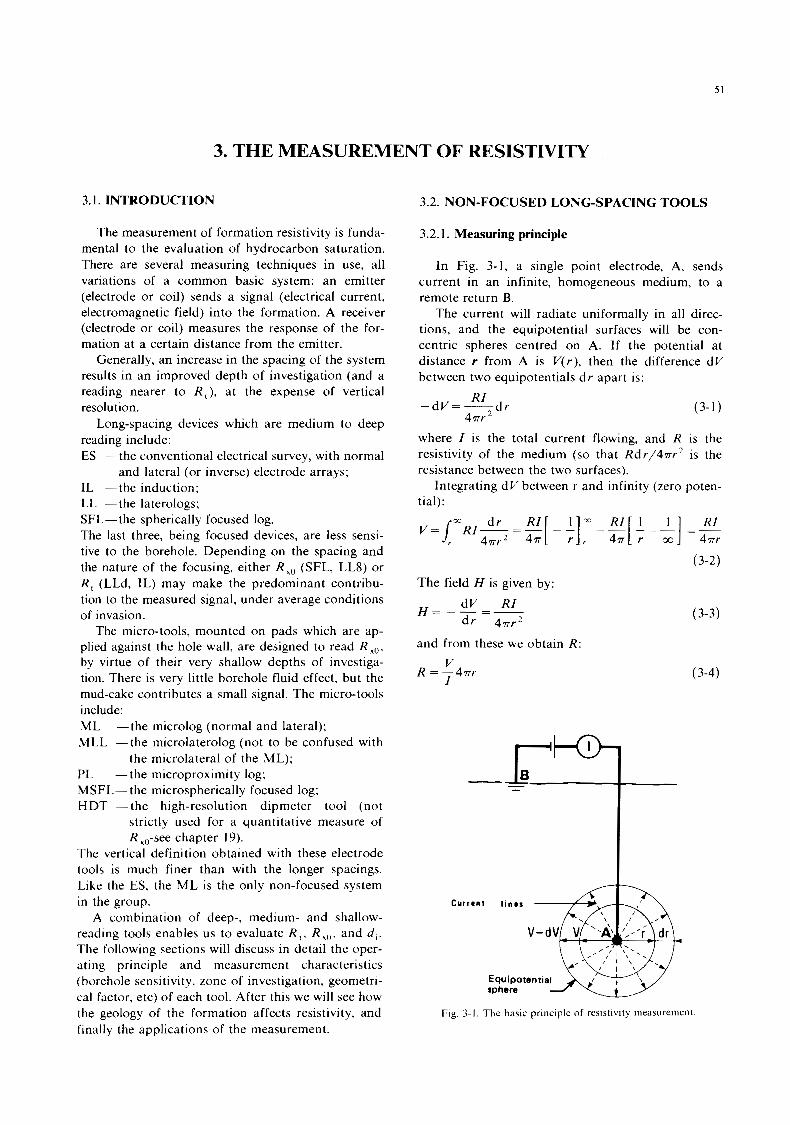
5 1
3. THE MEASUREMENT OF RESISTIVITY
3.1. INTRODUCTION
The measurement of formation resistivity is funda- mental to the evaluation of hydrocarbon saturation. There are several measuring techniques in use, all variations of a common basic system: an emitter (electrode or coil) sends a signal (electrical current, electromagnetic field) into the formation. A receiver (electrode or coil) measures the response of the for- mation at a certain distance from the emitter.
Generally, an increase in the spacing of the system results in an improved depth of investigation (and a reading nearer to R,), at the expense of vertical resolution.
Long-spacing devices which are medium to deep reading include: ES -the conventional electrical survey, with normal
IL -the induction; LL -the laterologs; SFL- the spherically focused log. The last three, being focused devices, are less sensi- tive to the borehole. Depending on the spacing and the nature of the focusing, either R,, (SFL, LL8) or R , (LLd, IL) may make the predominant contribu- tion to the measured signal, under average conditions of invasion.
The micro-tools, mounted on pads which are ap- plied against the hole wall, are designed to read R, , , by virtue of their very shallow depths of investiga- tion. There is very little borehole fluid effect, but the mud-cake contributes a small signal. The micro-tools include: ML MLL -the microlaterolog (not to be confused with
PL -the microproximity log; MSFL- the microspherically focused log; HDT -the high-resolution dipmeter tool (not
strictly used for a quantitative measure of R ,,,-see chapter 19).
The vertical definition obtained with these electrode tools is much finer than with the longer spacings. Like the ES, the ML is the only non-focused system in the group.
A combination of deep-, medium- and shallow- reading tools enables us to evaluate R , , R and d , . The following sections will discuss in detail the oper- ating principle and measurement characteristics (borehole sensitivity, zone of investigation, geometri- cal factor, etc) of each tool. After this we will see how the geology of the formation affects resistivity, and finally the applications of the measurement.
and lateral (or inverse) electrode arrays;
-the microlog (normal and lateral);
the microlateral of the ML);
3.2. NON-FOCUSED LONG-SPACING TOOLS
3.2.1. Measuring principle
In Fig. 3-1, a single point electrode, A, sends current in an infinite, homogeneous medium, to a remote return B.
The current will radiate uniformally in all direc- tions, and the equipotential surfaces will be con- centric spheres centred on A. If the potential at distance r from A is V(r), then the difference dV between two equipotentials d r apart is:
- d v = - d r
where I is the total current flowing, and R is the resistivity of the medium (so that Rdr /4r r2 is the resistance between the two surfaces).
Integrating dV between r and infinity (zero poten- tial):
d r RI 3c R I 1 1 RI
(3-1) R I
4 r r 2
v=J: R I G - z [ - : ] , - =&;I =4711.
(3-2) The field H is given by:
dV R I d r 4 r r 2
H = --=-
and from these we obtain R:
(3-3)
(3-4) V R = - 4 r r I
Current l i n e r
Equipotential sphere
Fig. 3- I . The basic principle of reslstivlty measurement.

52
A
(3-5)
Equations 3-4 and 3-5 suggest two ways of measuring the resistivity and these are discussed next.
3.2.1.1. The normal configuration
The measuring electrode M is situated close to the current electrode A, (Fig. 3-2a). A constant current I flows from A to the remote return 9. The potential V , of M is measured with respect to a reference electrode N (at zero potential) by means of a volt-me- ter. Although, theoretically, N should be on surface (at “infinity”), inductive phenomena necessitate plac- ing it downhole, but at a distance from M consider- ably greater than is A (one of the bridle electrodes, for instance) (Fig. 3-2b). From eq. 3-2:
RI
477AM v, == (3-6)
neglecting borehole effects, i.e. we assume an infinite homogeneous medium.
Since I is held constant, VM is proportional to R. 4 n m is the coefficient K , of the normal device:
AV R = K -
N I (3-7)
Thus a continuous recording of V , on an ap- propriate scale is a log of the resistivity. There are two conventional AM spacings for the normal:
AM= 16”, the “short normal”;
AM= 64’, the “medium normal”. -
generator
rc7-
Equipotential wherical surfaces
recorder
@lN
3.2.1.2. Lateral and inverse configurutions
In the lateral configuration (Fig. 3-3a), two mea- suring electrodes, M and N, are placed close together below A. The difference AV between the spherical equipotential surfaces on which M and N lie, is derived as follows:
RI V M = -
477232
VM is the potential at electrode M, from eq. 3-2. RI
V , =- 4aAN
VN is the potential at electrode N, from eq. 3-2.
- MN
AV=RI ~
4nAMAN (3-8)
~- The constant 4rAMAN/MN is the coefficient K , for the lateral device. So:
(3-9) AV
R=K,- I
The formation resistivity R is proportional to AV if the current is constant.
In practice, return electrode B is placed downhole. and a modified, but equivalent ‘‘inverse” configura- tion is used (Fig. 3-3b). The electrode pair A-B takes the place of M-N; however, by the principle of re- ciprocity the resistivity relationship derived above still holds, with measure return electrode N remote from M.
generator
\ \-
a) Scheme of the norm& b) Real configuration device principle
Fig. 3-2. The normal configuration.
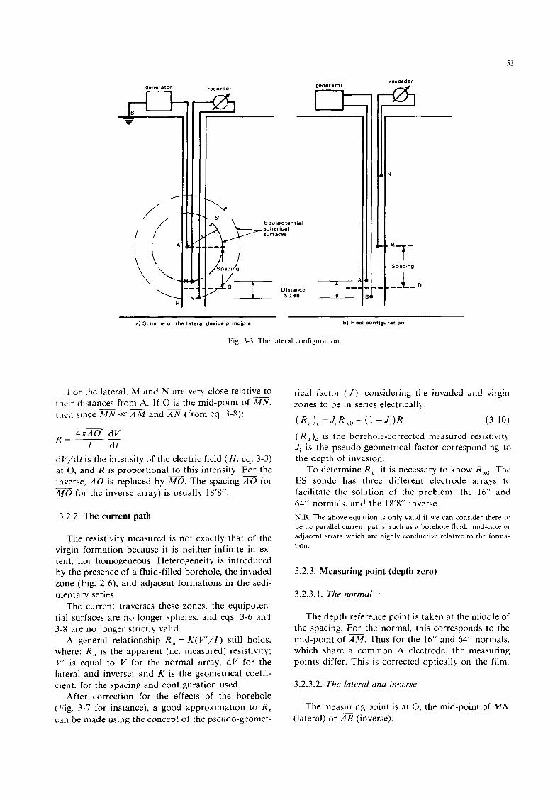
53
recorder generator
U
Equ ipoten tial spherical surfaces
Distance span
recorder
9
r-
N
7- Spacing
a) Scheme of the lateral device principle b) Real Configuration
Fig. 3-3. The lateral configuration
For the lateral, M and N are very close relative to their distances from A. If 0 is the mid-point of m, then since M N << AM and AN (from eq. 3-8):
4 a A ‘ dV I d l
R = - -
dV/dl is the intensity of the electric field ( H , eq. 3-3) at 0, and R is proportional to this intensity. For the inverse, is replaced by m. The spacing (or M O for the inverse array) is usually 18’8”. -
3.2.2. The current path
The resistivity measured is not exactly that of the virgin formation because it is neither infinite in ex- tent, nor homogeneous. Heterogeneity is introduced by the presence of a fluid-filled borehole, the invaded zone (Fig. 2-6), and adjacent formations in the sedi- mentary series.
The current traverses these zones, the equipoten- tial surfaces are no longer spheres, and eqs. 3-6 and 3-8 are no longer strictly valid.
A general relationship R , = K ( V’/Z) still holds, where: R;, is the apparent (i.e. measured) resistivity; V’ is equal to V for the normal array, dV for the lateral and inverse; and K is the geometrical coeffi- cient, for the spacing and configuration used.
After correction for the effects of the borehole (Fig. 3-7 for instance), a good approximation to R , can be made using the concept of the pseudo-geomet-
rical factor ( J ) , considering the invaded and virgin zones to be in series electrically:
( R , )c is the borehole-corrected measured resistivity. J , is the pseudo-geometrical factor corresponding t o the depth of invasion.
To determine R , , i t is necessary to know RK,,. The ES sonde has three different electrode arrays to facilitate the solution of the problem: the 16” and 64” normals, and the 18’8’’ inverse. N.B. The above equation is only valid i f we can consider there t o be no parallel current paths, such as a borehole fluid, mud-cake or adjacent strata which are highly conductive relative to the forma- tion.
3.2.3. Measuring point (depth zero)
3.2.3.1. The normal
The depth reference point is taken at the middle of the spacing. For the normal, this corresponds to the mid-point of AM. Thus for the 16” and 64” normals, which share a common A electrode, the measuring points differ. This is corrected optically on the film.
3.2.3.2. The lateral and inverse
The measuring point is at 0, the mid-point of M N (lateral) or AB (inverse).
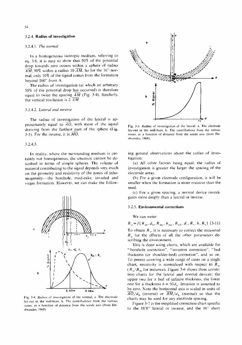
54
3.2.4. Radius of investigation
3.2.4.1. The normul a lilA
In a homogeneous isotropic medium. referring to eq. 3-6, i t is easy to show that 50% of the potential d rop towards zero occurs within a sphere of radius AM, 90% within a radius 10 AM. So for the 16”-nor- mal, only 10% of the signal comes from the formation beyond 160” from A.
The radius of investigation (at which an arbitrary 50% of the potential drop has occurred) is therefore equal to twice the spacing AM (Fig. 3-4). Similarly, the vertical resolution is 2 AM.
3.2.4.2. Lateral und inverse
The radius of investigation of the lateral is ap- proximately equal to m, with most of the signal deriving from the farthest part of the sphere (Fig. 3-5). For the inverse, it is m. 3.2.4.3.
In reality, where the surrounding medium is cer- tainly not homogeneous, the situation cannot be de- scribed in terms of simple spheres. The volume of material contributing to the signal depends very much on the geometry and resistivity of the zones of inho- mogeneity- the borehole, mud-cake, invaded and virgin formation. However, we can make the follow-
a
b
0 . 4 0 m 0 . 8 0 m
Fig. 3-4. Radius of investigation of the normal. a. The electrode lay-out in the well-bore. b. The contributions from the various zones. as a function of distance from the sonde axis (from De- sbrandes. 1968).
I .
Fig. 3-5. Radius of investigation of the lateral. a. The electrode lay-out in the well-bore. b. The contributions from the various zones, as a function of distance from the sonde axis (from De- sbrandes, 1968).
ing general observations about the radius of inves- tigation:
(a) All other factors being equal, the radius of investigation is greater the larger the spacing of the electrode array.
(b) For a given electrode configuration, i t will be smaller when the formation is more resistive than the mud.
(c) For a given spacing, a normal device investi- gates more deeply than a lateral or inverse.
3.2.5. Environmental corrections
To obtain R , , i t is necessary to correct the measured R , for the effects of all the other parameters de- scribing the environment.
This is done using charts. which are available for “ borehole correction”, “ invasion correction”, “ bed thickness (or shoulder-bed) correction”, and so on. To permit covering a wide range of cases on a single chart, resistivity is normalized with respect to R , ( R , / R ”, for instance). Figure 3-6 shows three correc- tion charts for the lateral and normal devices; the upper two for a bed of infinite thickness. the lower one for a thickness h = 50d,. Invasion is assumed to be zero. Note the horizontal axis is scaled in units of A / d , (inverse) or A / d , , (normal) so that the charts may be used for any electrode spacing.
Figure 3-7 is the simplified correction chart specific to the 18’8” lateral or inverse. and the 16” short
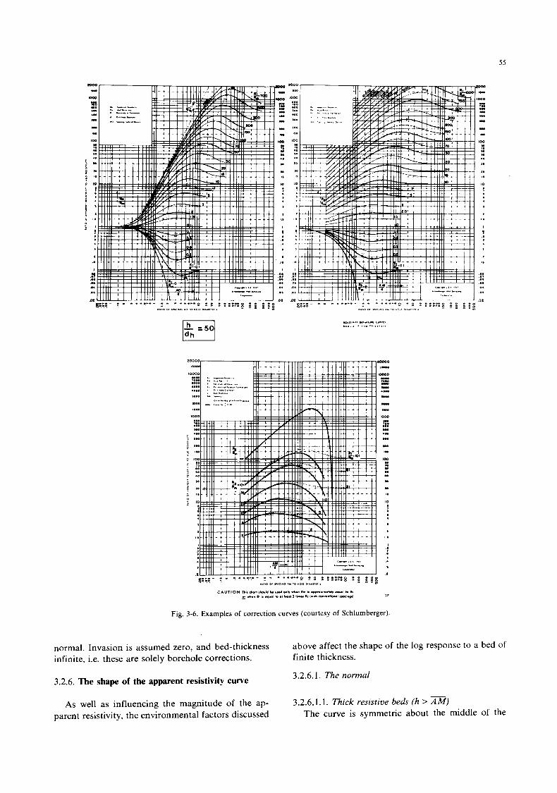
"%,,11"1,. DI... 1"" <"."L, ................... I " 1
Fig. 3-6. Examples of correction curves (courtesy of Schlumberger).
normal. Invasion is assumed zero, and bed-thickness infinite, i.e. these are solely borehole corrections.
3.2.6. The shape of the apparent resistivity curve
above affect the shape of the log response to a bed of finite thickness.
3.2.6.1. The normal
3.2.6.1.1. Thick resistive beds (h > AM) As well as influencing the magnitude of the ap- parent resistivity, the environmental factors discussed The curve is symmetric about the middle of the
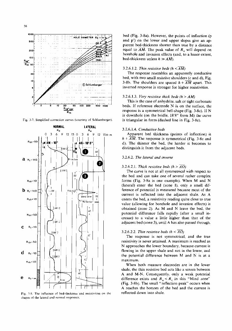
56
- _ - L l o w -- HOLE DIAMETER d $ = A
L . I . . . I . . . . . 1 I 5 0 0 - - ~
~
2 0 0 - - -
-~~ _* . . . . . , . . . . . . . . . -.
. . . . , . . , .
. . . . . . . . . . - , . . . ~*
. . .... ~ - 20- . . ’
. . . . . . .. - .
:l/s , , , , , ,I , , , , , , , , , ,.,l.ll, , I I I 2 5 10 20 50 100 200 500 1000
R16*COr
R m
Fig. 3-7 Simplified correction curves (courtesy of Schlumberger).
NORMAL LATERAL Ra Ra
0 3 6 9 12 1 5 0 3 6 9 12 1 5 0 m
Fig. 3-8. The influence of bed-thickness and resistivities on the shapes of the lateral and normal responses.
bed (Fig. 3-8a). However, the points of inflection (p and p’) on the lower and upper slopes give an ap- parent bed-thickness shorter than true by a distance equal to AM. The peak value of R , will depend on borehole and invasion effects (and, to a lesser extent, bed-thickness unless h >>AM).
3.2.6.1.2. Thin resistive be& (h <AM) The response resembles an apparently conductive
bed, with two small resistive shoulders (c and d), Fig. 3-8b. The shoulders are spaced h +AM apart. This inverted response is stronger for higher resistivities.
3.2.6.1.3. Very resistive thick be& (h > AM) This is the case of anhydrite, salt or tight carbonate
beds. If reference electrode N is on the surface, the response is a symmetrical bell-shape (Fig. 3-8e). If N is downhole (on the bridle, 18’8” from M) the curve is triangular in form (dashed line in Fig. 3-8e).
3.2.6.1.4. Conductive b e d Apparent bed thickness (points of inflection) is
h + AM. The response is symmetrical (Fig. 3-8c and d). The thinner the bed, the harder it becomes to distinguish it from the adjacent beds.
3.2.6.2, The lateral and inverse
3.2.6.2.1. Thick resistive beds (h > m) The curve is not at all symmetrical with respect to
the bed and can take one of several rather complex forms (Fig. 3-8a is one example). When M and N (lateral) enter the bed (zone I), only a small dif- ference of potential is measured because most of the current is reflected into the adjacent shale. As A enters the bed, a resistivity reading quite close to true value (allowing for borehole and invasion effects) is obtained (zone 2). As M and N leave the bed, the potential difference falls rapidly (after a small in- crease) to a value a little higher than that of the adjacent bed (zone 3), until A has also passed through.
3.2.6.2.2. Thin resistive beds (h < m) The response is not symmetrical, and the true
resistivity is never attained. A maximum is reached as N approaches the lower boundary, because current is flowing in the upper shale and not in the lower, and the potential difference between M and N is at a maximum.
When both measure electrodes are in the lower shale, the thin resistive bed acts like a screen between A and M-N. Consequently, only a weak potential difference exists and R , < R , in this “blind zone” (Fig. 3-8b). The small “reflection peak” occurs when A reaches the bottom of the bed and the current is reflected down into shale.
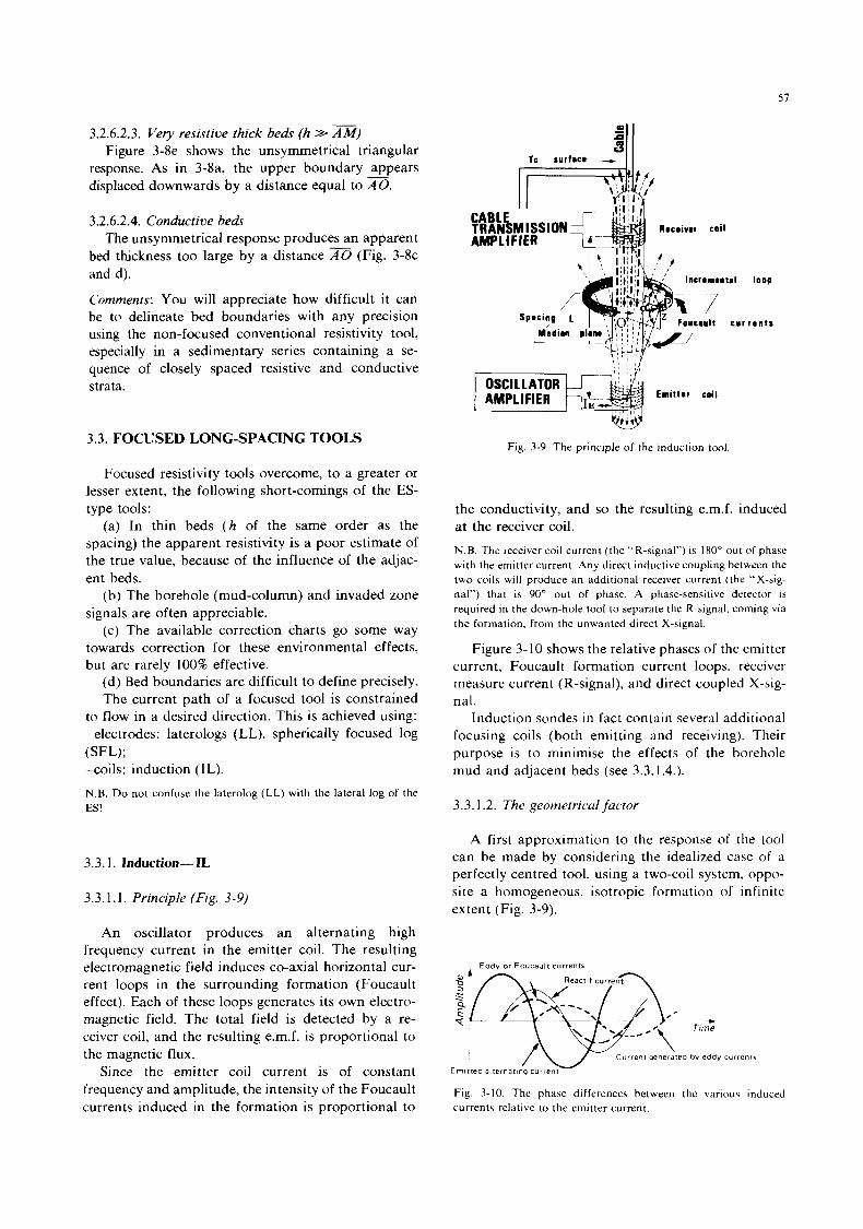
51
3.2.6.2.3. Very resistive thick beds (h B AM) Figure 3-8e shows the unsymmetrical triangular
response. As in 3-8a, the upper boundary appears displaced downwards by a distance equal to m. 3.2.6.2.4. Conductive beds
bed thickness too large by a distance and d).
Comments: You will appreciate how difficult it can be to delineate bed boundaries with any precision using the non-focused conventional resistivity tool, especially in a sedimentary series containing a se- quence of closely spaced resistive and conductive strata.
The unsymmetrical response produces an apparent (Fig. 3-8c
3.3. FOCUSED LONG-SPACING TOOLS
Focused resistivity tools overcome, to a greater or lesser extent, the following short-comings of the ES- type tools:
(a) In thin beds ( h of the same order as the spacing) the apparent resistivity is a poor estimate of the true value, because of the influence of the adjac- ent beds.
(b) The borehole (mud-column) and invaded zone signals are often appreciable.
(c) The available correction charts go some way towards correction for these environmental effects, but are rarely 100% effective.
(d) Bed boundaries are difficult to define precisely. The current path of a focused tool is constrained
to flow in a desired direction. This is achieved using: -electrodes: laterologs (LL), spherically focused log (SFL); -coils: induction (IL). N.B. Do not confuse the laterolog (LL) with the lateral log of the ES!
3.3. I . Induction-IL
3.3.1.1. Principle (Fig. 3-9)
An oscillator produces an alternating high frequency current in the emitter coil. The resulting electromagnetic field induces co-axial horizontal cur- rent loops in the surrounding formation (Foucault effect). Each of these loops generates its own electro- magnetic field. The total field is detected by a re- ceiver coil, and the resulting e.m.f. is proportional to the magnetic flux.
Since the emitter coil current is of constant frequency and amplitude, the intensity of the Foucault currents induced in the formation is proportional to
Racaivrr coil
Emit1 a r coi I
Fig. 3-9. The principle of the induction tool.
loop
r a n t s
the conductivity, and so the resulting e.m.f. induced at the receiver coil. N.B. The receiver coil current (the "R-signal") is 180" out of phase with the emitter current. Any direct inductive coupling between the two coils will produce an additional receiver current (the "X-sig- nal") that is 90" out of phase. A phase-sensitive detector i s required in the down-hole tool to separate the R-signal. coming via the formation, from the unwanted direct X-signal.
Figure 3-10 shows the relative phases of the emitter current, Foucault formation current loops, receiver measure current (R-signal), and direct coupled X-sig- nal.
Induction sondes in fact contain several additional focusing coils (both emitting and receiving). Their purpose is to minimise the effects of the borehole mud and adjacent beds (see 3.3.1.4.).
3.3.1.2. The geometrical factor
A first approximation to the response of the tool can be made by considering the idealized case of a perfectly centred tool, using a two-coil system. oppo- site a homogeneous, isotropic formation of infinite extent (Fig. 3-9).
Eddy or Foucault currents
Emit ted alternating A current-
Fig. 3-10. The phase differences between the various induced currents relative to the emitter current.
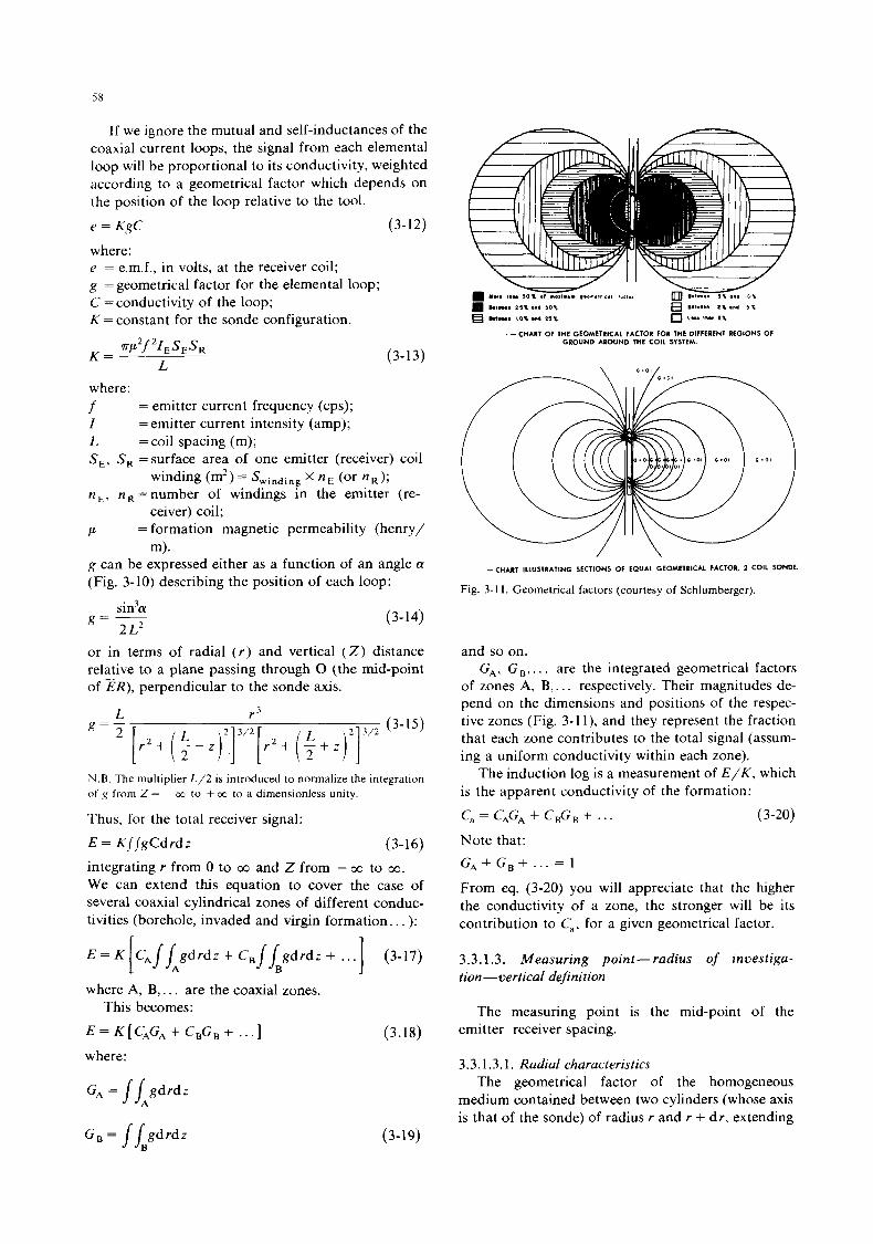
58
If we ignore the mutual and self-inductances of the coaxial current loops, the signal from each elemental loop will be proportional to its conductivity, weighted according to a geometrical factor which depends on the position of the loop relative to the tool. e = KgC (3-12)
where: e = e.m.f., in volts, at the receiver coil; g =geometrical factor for the elemental loop; C =conductivity of the loop; K =constant for the sonde configuration.
(3-13)
where: f = emitter current frequency (cps); I =emitter current intensity (amp); L = coil spacing (m); S, , S , =surface area of one emitter (receiver) coil
n E , n R =number of windings in the emitter (re-
P = formation magnetic permeability (henry/
g can be expressed either as a function of an angle a (Fig. 3-10) describing the position of each loop:
winding (m2)= Swinding X n E (or n R ) ;
ceiver) coil;
m).
sin3a g = 2 2L
(3-14)
or in terms of radial ( r ) and vertical ( Z ) distance relative to a plane passing through 0 (the mid-point of m), perpendicular to the sonde axis.
N.B. The multiplier L / 2 is introduced to normalize the integration o f g from Z = ~ 03 to + M to a dimensionless unity.
Thus, for the total receiver signal:
E = K//gCdrdz (3-16) integrating r from 0 to 00 and Z from - 00 to 00.
We can extend this equation to cover the case of several coaxial cylindrical zones of different conduc- tivities (borehole, invaded and virgin formation.. . ):
E = K [ CA// gdrdz + C,/Lgdrdz + . . .] (3-17) A
where A, B, . . . are the coaxial zones. This becomes:
E = K [ C,C, + C,G, + . . . ] (3.18) where:
G, = / L g d r d r
G, = /Lgdrdz (3-19)
I I
- CHART O F THE GEOMETRICAL FACTOR FOR THE DIFFERENT REGIONS Of GROUND AROUND THE COIL SYSTEM.
\ G . O I / - \,I/- A\l . I//- \
/ \ -CHART ILLUSTRATING SECTIONS OF EQUAL GEOMETRICAL FACTOR, 2 COIL SONDE.
Fig. 3-1 1. Geometrical factors (courtesy of Schlumberger).
and so on. CAI G,, . . . are the integrated geometrical factors
of zones A, B,. . . respectively. Their magnitudes de- pend on the dimensions and positions of the respec- tive zones (Fig. 3-1 l), and they represent the fraction that each zone contributes to the total signal (assum- ing a uniform conductivity within each zone).
The induction log is a measurement of E / K , which is the apparent conductivity of the formation:
c, = C,G, + C,G, + . . . (3-20)
Note that: GA+GG,+ . . .= 1
From eq. (3-20) you will appreciate that the higher the conductivity of a zone, the stronger will be its contribution to C,, for a given geometrical factor.
3.3.1.3. Measuring point-radius of investiga- tion -vertical definition
The measuring point is the mid-point of the emitter-receiver spacing.
3.3.1.3.1. Radial characteristics The geometrical factor of the homogeneous
medium contained between two cylinders (whose axis is that of the sonde) of radius r and r + dr , extending
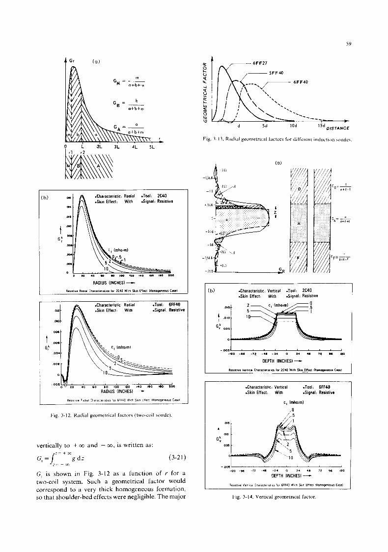
59
0 i ai 3L 4L 5L
b)
t G :
.Characteristic: Radial .Tool: 2C40 .Signal: Resistive
RAOIUS (INCHES) -t
R~rir t iui Radial Charartirirticr lor 2C40 With Shin €flirt lHomoglncour C a d
.Characteristic Radial .Tool 6FF40 -21 A .Skin Effect With .Signal Resistive
Fig. 3- 12. Radial geometrical factors (two-coil sonde).
vertically to + co and - 00, is written as:
R d z (3-21)
G, is shown in Fig. 3-12 as a function of r for a two-coil system. Such a geometrical factor would correspond to a very thick homogeneous formation, so that shoulder-bed effects were negligible. The major
4
5d 0 IS TA NC E d 5d 1 Od
Fig. 3- 13. Radial geometrical factors f o r different induction aundes.
1
(b) .Characteristic Vertical .Tool 2C40 .Skin Effect With .Signal Resistive
.Characteristic Vertical .Tool 6FF40
.Skin Effect With .Signal Resistive
c t Imhorrn)
as
ao
G: 008
0
420 -98 -I2 -40 - 2 4 0 2 4 48 I2 % 120
OEPTH (INCHES) - R e r ~ r l i v s V e r l ~ c a l Chiracler,rlirr l o r 6FF40 W i l h Skin E l l i r l IHomogmews Caral
Fig. 3-14. Vertical geometrical factor
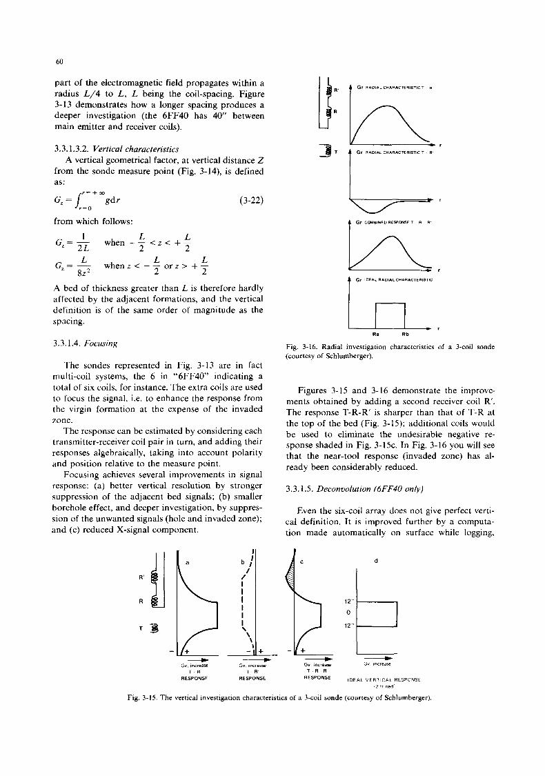
60
part of the electromagnetic field propagates within a radius L/4 to L, L being the coil-spacing. Figure 3-13 demonstrates how a longer spacing produces a deeper investigation (the 6FF40 has 40” between main emitter and receiver coils).
3.3.1.3.2. Vertical characteristics A vertical geometrical factor, at vertical distance 2
from the sonde measure point (Fig. 3-14), is defined as:
r - + 00
G, = gdr (3 -22) L o
from w l c h follows:
L L when -- < z < + - 2 L 2 2
1 G = -
L L L whenz< -- o r z > + - G,= - 82 * 2 2
A bed of thickness greater than L is therefore hardly affected by the adjacent formations, and the vertical definition is of the same order of magnitude as the spacing.
3.3.1.4. Focusing
The sondes represented in Fig. 3-13 are in fact multi-coil systems, the 6 in “6FF40” indicating a total of six coils, for instance. The extra coils are used to focus the signal, i.e. to enhance the response from the virgin formation at the expense of the invaded zone.
The response can be estimated by considering each transmitter-receiver coil pair in turn, and adding their responses algebraically, taking into account polarity and position relative to the measure point.
Focusing achieves several improvements in signal response: (a) better vertical resolution by stronger suppression of the adjacent bed signals; (b) smaller borehole effect, and deeper investigation, by suppres- sion of the unwanted signals (hole and invaded zone); and (c) reduced X-signal component.
’ + b Gv. - increase
T R RESPONSE
\ \ \ \ ! Gv. -+ T - + increase R ’
RESPONSE
Gr RADIALCHARACTERISTIC T R
Gr RADIAL CHARACTERISTIC T R’
Gr COMBINED RESPONSE T ~ R ~ R’
I
Gr IDEAL RADIAL CHARACTERISTIC t
Ra Rb
Fig. 3-16. Radial investigation characteristics (courtesy of Schlurnberger).
r
of a 3-coil sonde
Figures 3-15 and 3-16 demonstrate the improve- ments obtained by adding a second receiver coil R’. The response T-R-R’ is sharper than that of T-R at the top of the bed (Fig. 3-15); additional coils would be used to eliminate the undesirable negative re- sponse shaded in Fig. 3- 15c. In Fig. 3- 16 you will see that the near-tool response (invaded zone) has al- ready been considerably reduced.
3.3. I .5. Deconvolution (6FF40 onlyl
Even the six-coil array does not give perfect verti- cal definition. It is improved further by a computa- tion made automatically on surface while logging,
Gv mcrease Gv increase
T R R ’
I D E A L V E R l l C A L RESPONSE I 2 11 hedl
Fig. 3-15. The vertical investigation characteristics of a 3-coil sonde (courtesy of Schlumberger).
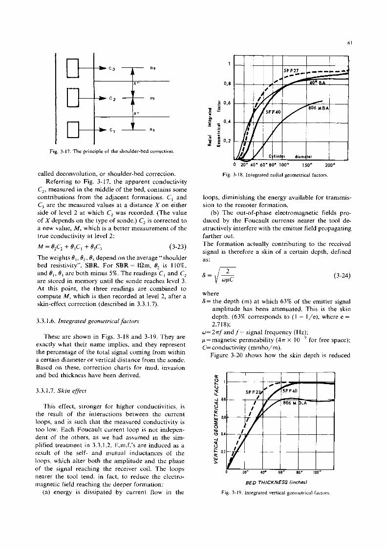
Fig. 3-17. The principle of the shoulder-bed correction.
called deconvolution, or shoulder-bed correction. Referring to Fig. 3- 17, the apparent conductivity
C,, measured in the middle of the bed, contains some contributions from the adjacent formations. C, and C, are the measured values at a distance X on either side of level 2 at which C, was recorded. (The value of X depends on the type of sonde.) C, is corrected to a new value, M , which is a better measurement of the true conductivity at level 2 :
M = e,c, + B,C, + e,c, (3-23)
The weights B , , B,, 0, depend on the average "shoulder bed resistivity", SBR. For SBR = lQm, Br is 1 lo%, and B , , B, are both minus 5%. The readings C, and C, are stored in memory until the sonde reaches level 3. At this point, the three readings are combined to compute M , which is then recorded at level 2, after a skin-effect correction (described in 3.3.1.7).
3.3.1.6. Integrated geometrical factors
These are shown in Figs. 3-18 and 3-19. They are exactly what their name implies, and they represent the percentage of the total signal coming from within a certain diameter or vertical distance from the sonde. Based on these, correction charts for mud, invasion and bed thickness have been derived.
3.3.1.7. Skin effect
This effect, stronger for higher conductivities, is the result of the interactions between the current loops, and is such that the measured conductivity is too low. Each Foucault current loop is not indepen- dent of the others, as we had assumed in the sim- plified treatment in 3.3.1.2. E.m.f.'s are induced as a result of the self- and mutual inductances of the loops, which alter both the amplitude and the phase of the signal reaching the receiver coil. The loops nearer the tool tend, in fact, to reduce the electro- magnetic field reaching the deeper formation:
(a) energy is dissipated by current flow in the
61
0 20" 40" 60"80' 100" 150" 200"
Fig. 3- 18. Integrated radial geometrical factors
loops, diminishing the energy available for transmis- sion to the remoter formation.
(b) The out-of-phase electromagnetic fields pro- duced by the Foucault currents nearer the tool de- structively interfere with the emitter field propagating farther out. The formation actually contributing to the received signal is therefore a skin of a certain depth, defined as:
(3-24)
where 6 = the depth (m) at which 63% of the emitter signal
amplitude has been attenuated. This is the skin depth. (63% corresponds to ( 1 - I/e), where e =
2.7 18); w= 277f and f = signal frequency (Hz); p=magnetic permeability (4a x l o p 7 for free space); C= conductivity (mmho/m).
Figure 3-20 shows how the skin depth is reduced
a e l
- s 8
9
c, T cc 4 0.9
a 06
lu 0 0.4 4
i2 0 2 rt
0 20" 40. 60" no' 100"
BED THICKNESS (inches)
Flg 3-19 Integrated vertical geometrical fdctors
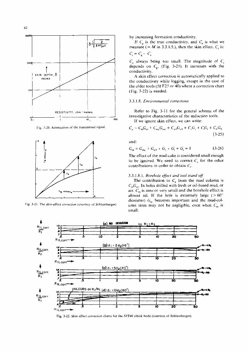
RESISTIV ITY, ohm - meters
I 1 0. I I lo , 100
10
Fig. 3-20. Attenuation of the transmitted signal.
t. b
E
_ - T I
I cg mhos/,- I
14
Fig. 3-21. The skin-effect correction (courtesy of Schlumberger).
by increasing formation conductivity. If C, is the true conductivity, and C, is what we
measure (= M in 3.3.1.5.), then the skin effect, C, is: c, = c, - c, C, always being too small. The magnitude of C, depends on C,, (Fig. 3-21). I t increases with the conductivity.
A skin effect correction is automatically applied to the conductivity while logging, except in the case of the older tools (5FF27 or 40) where a correction chart (Fig. 3-22) is needed.
3.3.1.8. Enoironmental corrections
Refer to Fig. 3-1 1 for the general schema of the
If we ignore skin effect, we can write: investigative characteristics of the induction tools.
C, = C,G,,, + C,,,G,,, + C,,,G,, + C,G, + CtG, + CSG, (3-25)
and :
G, + G,, + G,, + G, + G, + G, = 1 (3-26)
The effect of the mud-cake is considered small enough to be ignored. We need to correct C, for the other contributions in order to obtain C,.
3.3.1.8.1. Borehole effect and tool stand-off The contribution to Ca from the mud column is
C,G,,. In holes drilled with fresh or oil-based mud, or air, C, is zero or very small and the borehole effect is almost nil. If the hole is extremely large ( > 60” diameter) G, becomes important and the mud-col- umn term may not be negligible, even when C, is small.
4 R A c o r r
R t
4 rc LO .S -00 1 .?
J - H I L c o r e
Fig. 3-22. Skin effect correction charts for the 5FF40 (thick beds) (courtesy of Schlumberger).
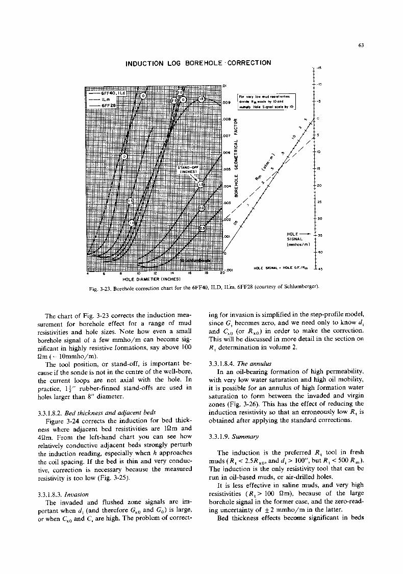
63
INDUCTION LOG BOREHOLE .CORRECTION - -15
---I0
- - - 5
0
5
-- 10
IS
-- 20
-- 25
--30
35
- - 4 0
1 4 5
HOLE DIAMETER (INCHES)
Fig. 3-23. Borehole correction chart for the 6FF40, ILD, IL‘m, 6FF28 (courtesy of Schlumberger).
The chart of Fig. 3-23 corrects the induction mea- surement for borehole effect for a range of mud resistivities and hole sizes. Note how even a small borehole signal of a few mmho/m can become sig- nificant in highly resistive formations, say above 100 9 m ( = IOmmho/m).
The tool position, or stand-off, is important be- cause if the sonde is not in the centre of the well-bore, the current loops are not axial with the hole. In practice, 1 i’’ rubber-finned stand-offs are used in holes larger than 8” diameter.
3.3.1.8.2. Bed thickness and adjacent beds Figure 3-24 corrects the induction for bed thick-
ness where adjacent bed resistivities are l a m and 49m. From the left-hand chart you can see how relatively conductive adjacent beds strongly perturb the induction reading, especially when h approaches the coil spacing. If the bed is thin and very conduc- tive, correction is necessary because the measured resistivity is too low (Fig. 3-25).
3.3.1.8.3. Znvasion The invaded and flushed zone signals are im-
portant when d i (and therefore G,, and Go) is large, or when C,, and Ci are high. The problem of correct-
ing for invasion is simplified in the step-profile model, since Gi becomes zero, and we need only to know d i and C,, (or Rxo) in order to make the correction. This will be discussed in more detail in the section on R, determination in volume 2.
3.3.1.8.4. The annulus In an oil-bearing formation of high permeability,
with very low water saturation and high oil mobility, it is possible for an annulus of high formation water saturation to form between the invaded and virgin zones (Fig. 3-26). This has the effect of reducing the induction resistivity so that an erroneously low R, is obtained after applying the standard corrections.
3.3.1.9. Summary
The induction is the preferred R, tool in fresh muds (R, < 2.5RX,, and di > loo”, but R, < 500 R,,,). The induction is the only resistivity tool that can be run in oil-based muds, or air-drilled holes.
It is less effective in saline muds, and very hlgh resistivities ( R , > 100 Qm), because of the large borehole signal in the former case, and the zero-read- ing uncertainty of f 2 mmho/m in the latter.
Bed thickness effects became significant in beds
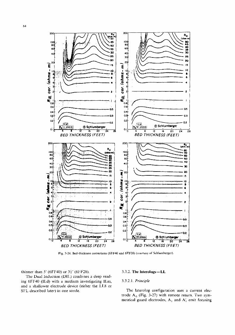
64
0.6
a2
- 1 O h m 01
BED THICKNESS (FEET)
c 2 4 '4'
0.3
a2- y h2 m 0 Schlumhrger - __,- ai 0 4 8 12 16 I 20 I 24 2 8
BED THICKNESS (FEET)
200 - - too: 80 : 60-
40 - I . -------&I
BED THICKNESS (FEET) BED THICKNESS (FEET) -
Fig. 3-24. Bed-thickness corrections (6FF40 and 6FF28) (courtesy of Schlumberger).
thinner than 5' (6FF40) or 34' (6FF28). The Dual Induction (DIL) combines a deep read-
ing 6FF40 (ILd) with a medium investigating ILm, and a shallower electrode device (either the LL8 or SFL described later) in one sonde.
3.3.2. The laterologs-LL
3.3.2.1. Principle
The laterolog configuration uses a current elec- trode A, (Fig. 3-27) with remote return. Two sym- metrical guard electrodes, A, and A', emit focusing
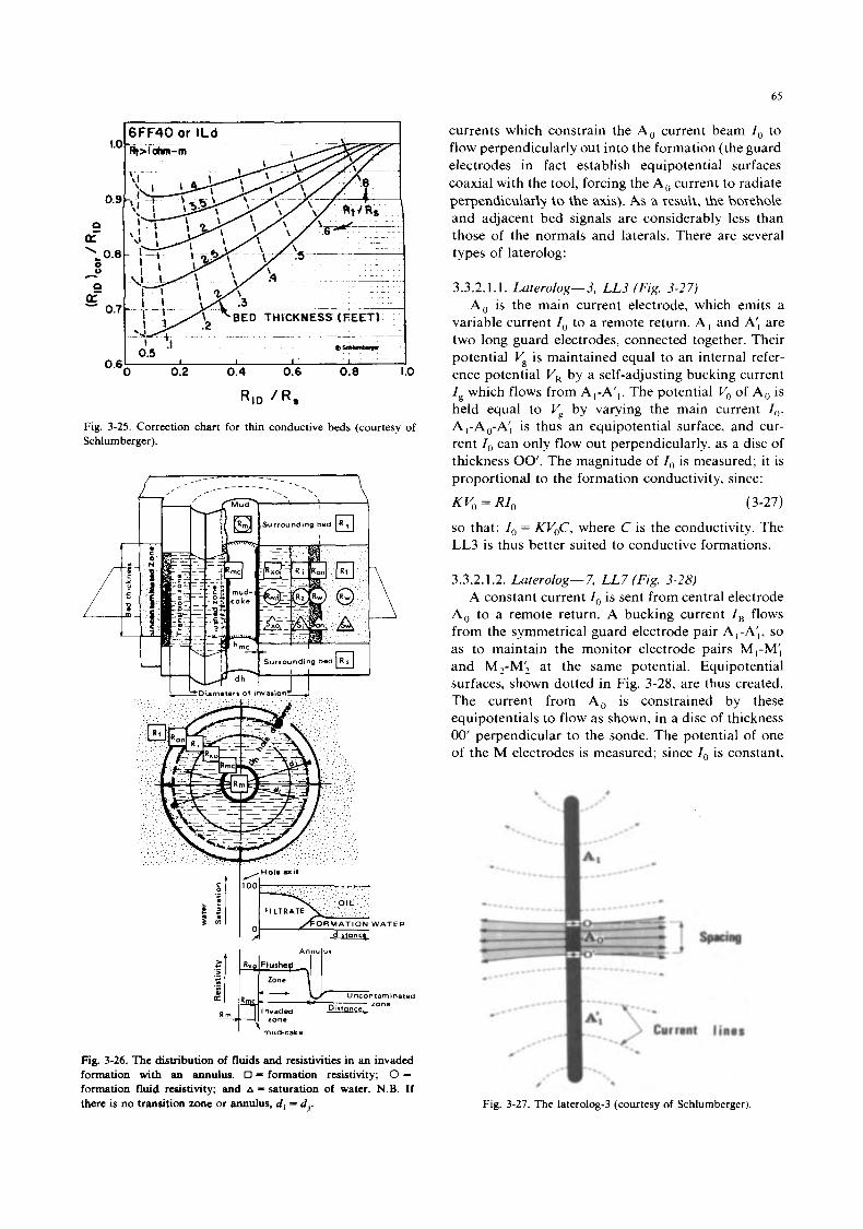
65
16FF40 or ILd I
Q- ‘ :I
0.5 1 1
0 0.2 0.4 0.6 0.8 I .o
RID ’ R s
0.6
Fig. 3-25. Correction chart for thin conductive beds (courtesy of Schlumberger).
,? ‘I h a i t
FILTRATE
ORMATION W A T E R
U nconraminated lone
Distance,
Fig. 3-26. The distribution of fluids and resistivities in an invaded formation with an annulus. 0 = formation resistivity; 0 =
formation fluid resistivity; and A-saturation of water. N.B. If there is no transition mne or annulus, di = d,.
currents which constrain the A, current beam I, to flow perpendicularly out into the formation (the guard electrodes in fact establish equipotential surfaces coaxial with the tool, forcing the A, current to radiate perpendicularly to the axis). As a result, the borehole and adjacent bed signals are considerably less than those of the normals and laterals. There are several types of laterolog:
3.3.2.1.1. Laterolog-3, LL3 (Fig. 3-27) A, is the main current electrode, which emits a
variable current I , to a remote return. A , and A‘, are two long guard electrodes, connected together. Their potential V, is maintained equal to an internal refer- ence potential V, by a self-adjusting bucking current Ig which flows from A,-A’,. The potential yl of A, is held equal to Vg by varying the main current I ( ) . A,-A,-A‘, is thus an equipotential surface, and cur- rent I , can only flow out perpendicularly, as a disc of thickness 00’. The magnitude of I , is measured; it is proportional to the formation conductivity, since:
KV, = RI, (3-27)
so that: I, = KV,C, where C is the conductivity. The LL3 is thus better suited to conductive formations.
3.3.2.1.2. Laterolog- 7, LL7 (Fig. 3-28) A constant current I , is sent from central electrode
A, to a remote return. A bucking current I , flows from the symmetrical guard electrode pair A,-A‘,, so as to maintain the monitor electrode pairs MI-M’, and M,-M; at the same potential. Equipotential surfaces, shown dotted in Fig. 3-28, are thus created. The current from A, is constrained by these equipotentials to flow as shown, in a disc of thickness 00’ perpendicular to the sonde. The potential of one of the M electrodes is measured; since I,, is constant,
spreins
l ines
Fig. 3-27. The laterolog-3 (courtesy of Schlumberger).
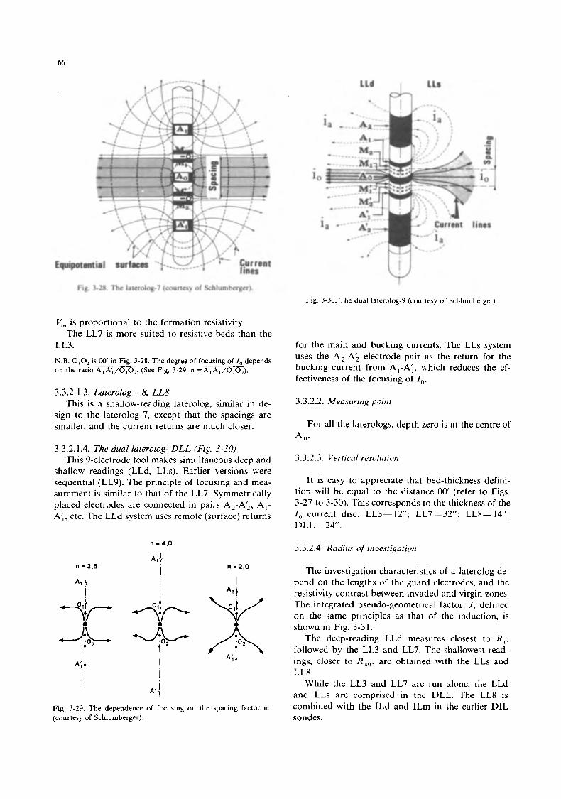
66
Fig. 3-28. The laterolog-7 (courtesy of Schlumberger).
V, is proportional to the formation resistivity.
LL3. The LL7 is more suited to resistive beds than the
__ N.B. O,O, is 00‘ in Fig. 3-28. The degree of focusing of I , depends on the ratio A,A’,/O,O,. (See Fig. 3-29, n =A,A’, /0,02).
-__ ~ _ _
3.3.2.1.3. Laterolog-8, LL8 This is a shallow-reading laterolog, similar in de-
sign to the laterolog 7, except that the spacings are smaller. and the current returns are much closer.
3.3.2.1.4. The dual laterolog-DLL (Fig. 3-30) This 9-electrode tool makes simultaneous deep and
shallow readings (LLd, LLs). Earlier versions were sequential (LL9). The principle of focusing and mea- surement is similar to that of the LL7. Symmetrically placed electrodes are connected in pairs A,-A;, A,- A’,, etc. The LLd system uses remote (surface) returns
n = 4,O
A,!
I n = 2 , 5 n =2 ,0
Fig. 3-29. The dependence of focusing on the spacing factor n. (courtesy of Schlumberger).
Fig. 3-30. The dual laterolog-9 (courtesy of Schlumberger).
for the main and bucking currents. The LLs system uses the A,-A; electrode pair as the return for the bucking current from A,-A’,, which reduces the ef- fectiveness of the focusing of I , .
3.3.2.2. Measuring point
For all the laterologs, depth zero is at the centre of ‘40.
3.3.2.3. Vertical resolution
It is easy to appreciate that bed-thickness defini- tion will be equal to the distance 00’ (refer to Figs. 3-27 to 3-30). This corresponds to the thickness of the I , current disc: LL3- 12”; LL7-32”; LL8- 14”; DLL-24”.
3.3.2.4. Radius of investigation
The investigation characteristics of a laterolog de- pend on the lengths of the guard electrodes, and the resistivity contrast between invaded and virgin zones. The integrated pseudo-geometrical factor, J , defined on the same principles as that of the induction, is shown in Fig. 3-31.
The deep-reading LLd measures closest to R , , followed by the LL3 and LL7. The shallowest read- ings, closer to R, , , are obtained with the LLs and LL8.
While the LL3 and LL7 are run alone, the LLd and LLs are comprised in the DLL. The LL8 is combined with the ILd and ILm in the earlier DIL sondes.
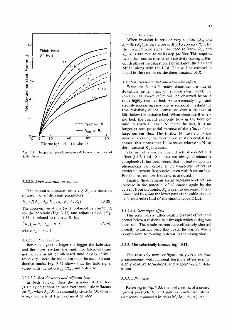
67
1.0
7
b ,.8 0 0 k
0 0 L . 6 - Q)
0
- .- 4-
E
s 64-
a
-0 3 Q) v)
.2
-
-
-
r I I I
O:, 8 $0 40 60 80
Diameter d i ( inches 1
Fig. 3-31, Integrated pseudo-geometrical factors (courtesy of Schlumberger).
3.3.2.5. Environmental corrections
The measured apparent resistivity R , is a function of a number of different parameters:
R , =f(R . , , d,, R,,, d , , R, , h , R , ) (3-28)
The apparent resistivity ( R , ) c obtained by correcting for the borehole (Fig. 3-32) and adjacent beds (Fig. 3-33), is related to the true R , by:
( R , )' = R x o J,, + R t J, (3-29)
where J,, + J , = 1.
3.3.2.5.1. The borehole Borehole signal is larger the bigger the hole size,
and the more resistant the mud. The laterologs can- not be run in air or oil-based mud having infinite resistivity-here the induction must be used. In con- ductive muds, Fig. 3-32 shows that the hole signal varies with the ratio R,,/R,, and hole size.
3.3.2.5.2. Bed thickness and adjacent beds In beds thicker than the spacing of the tool
(3.3.2.3.) neighbouring beds exert very little influence on R , , when R , / R , is reasonably close to 1.0. Other- wise, the charts of Fig. 3-33 must be used.
3.3.2.5.3. Invasion When invasion is zero or very shallow (.Ix, and
f, = 0), ( R a ) = is very close to R , . To correct ( Ra)= for the invaded zone signal, we need to know R, , and Jxo. J , is assumed to be 0 (step profile). This requires two other measurements of resistivity having differ- ent depths of investigation. For instance, the LLs and MSFL along with the LLd. This will be covered in detail in the section on the determination of R , .
3.3.2.5.4. Delaware and anti-Delaware effects When the B and N return electrodes are located
downhole rather than on surface (Fig. 3-34), the so-called Delaware effect will be observed below a thick highly resistive bed. An erroneously high, and steadily increasing resistivity is recorded, masking the true resistivity of the formations over a distance of 80ft below the resistive bed. When electrode B enters the bed, the current can only flow in the borehole mud to reach B. Once N enters the bed, i t is no longer at zero potential because of the effect of this large current flux. The further N travels into the resistive section, the more negative its potential be- comes; this means that & increases relative to N, so the measured R , increases.
The use of a surface current return reduces this effect (LL7, LLd), but does not always eliminate i t completely. I t has been found that mutual inductance phenomena can create a Delaware-type effect at moderate current frequencies, even with B on surface. For this reason, low frequencies are used.
Finally, there remains an anti-Delaware effect; an increase in the potential of N, caused again by the current from the sonde. R , is seen to decrease. This is minimized by using the lower part of the cable armour as N electrode (LLd of the simultaneous DLL).
3.3.2.5.5. Groningen effect This resembles a rather weak Delaware effect, and
occurs below a resistive bed through which casing has been run. The sonde currents are effectively shorted directly to surface once they reach the casing, which is equivalent to moving B down to the casing-shoe.
3.3.3. The spherically focused log-SFL
This relatively new configuration gives a shallow measurement, with minimal borehole effect even in highly resistive formations, and a good vertical defi- nition.
3.3.3.1. Principle
Referring to Fig. 3-35, the tool consists of a central current electrode A, and eight symmetrically placed electrodes, connected in pairs M,-M',. A,-A',, etc.
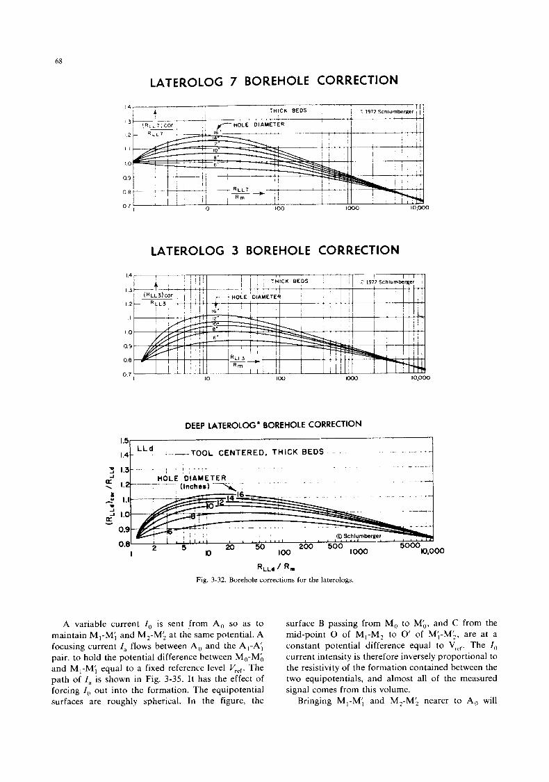
68
LATEROLOG 7 BOREHOLE CORRECTION
14
1 3
I 2
I 1
I 0
09
0 8
07 0
LATEROLOG 3 BOREHOLE CORRECTION
10 lO.000
DEEP LATEROLOG* BOREHOLE CORRECTION
1.5 . _ _ * _ I .4 ----TOOL CENTERED, THICK BEDS - -
RLLI 1 Rm Fig. 3-32. Borehole corrections for the laterologs.
A variable current I,, is sent from A,, so as to maintain M,-M’, and M,-M; at the same potential. A focusing current I , flows between A,, and the A,-A’, pair, to hold the potential difference between M,-M’, and M,-M’, equal to a fixed reference level Vref. The path of I , is shown in Fig. 3-35. It has the effect of forcing I , out into the formation. The equipotential surfaces are roughly spherical. In the figure, the
surface B passing from M, to M;, and C from the mid-point 0 of M,-M, to 0’ of M’,-M;, are at a constant potential difference equal to Vref. The I , current intensity is therefore inversely proportional to the resistivity of the formation contained between the two equipotentials, and almost all of the measured signal comes from this volume.
Bringing M,-M’, and M,-M; nearer to A, will
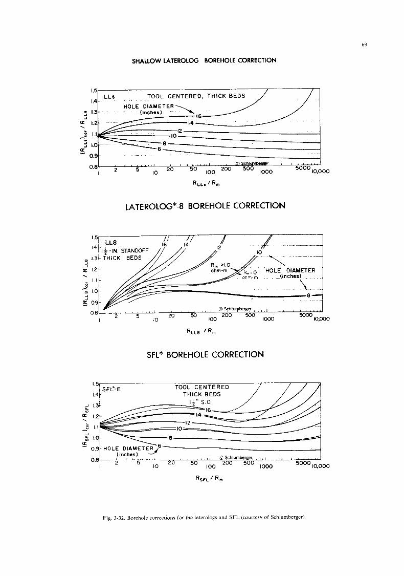
69
SHALLOW LATEROLOG BOREHOLE CORRECTION
1.5 LLS TOOL CENTERED, THICK BEDS
14 HOLE DIAMETER
f 1.3- - (Inches) L,6 / J
. . : 1.1,
i 1.0 1
K I
0.9 1 , @ S c h l m w e r J
2o 50 100 2oo 500 1000 5000 l0,Ooo 0.d 2
' ' ' ' ""
I 10
R L L ~ 1 R m
LATEROLOG"8 BOREHOLE CORRECTION
-
_ - - -
\- HOLE DIAMETER
(inches) _ _ - \-- -
8- . . , 'QSchlu~berger , , ,
- d o 9 y/ 5ooo
QOOo 200 500 ,ooo
5o 100 20
10 O8 2 ' " " . !
I
SFL" BOREHOLE CORRECTION
TOOL CENTERED
RSFL R m
Fig. 3-32. Borehole corrections for the laterologs and SFL (courtesy of Schlurnberger).
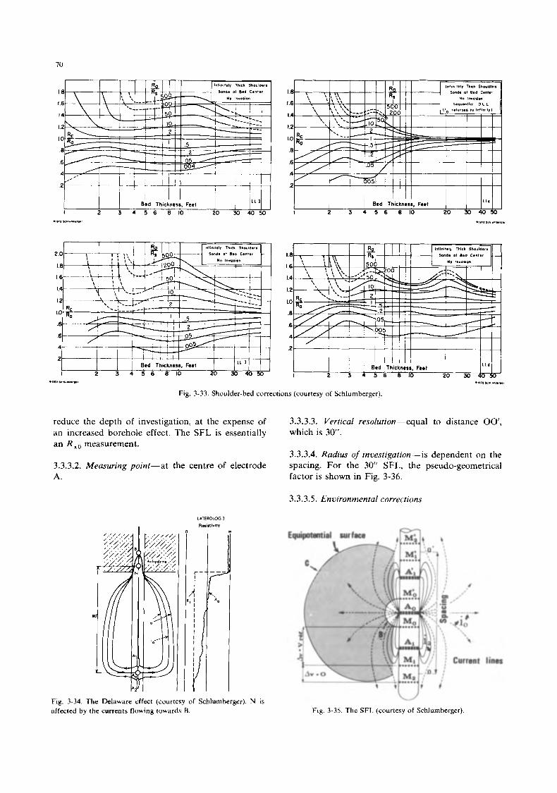
70
I
Bed 1 Thickness. 1 1 1 1 Feet L L I Bed Thicknear. Feet
I 2 3 4 5 6 8 1 0 20 m 4 0 w
Fig. 3-33. Shoulder-bed corrections (courtesy of Schlumberger)
reduce the depth of investigation, at the expense of an increased borehole effect. The SFL is essentially an R , , measurement.
3.3.3.2. Measuring point-at the centre of electrode A.
3.3.3.3. Vertical resolution-equal to distance 00', which is 30".
3.3.3.4. Radius of investigation-is dependent on the spacing. For the 30" SFL, the pseudo-geometrical factor is shown in Fig. 3-36.
3.3.3.5. Environmental corrections
LATEROLOG 3
Rnimwify 0 DI
Fig. 3-34. The Delaware effect (courtesy of Schlumberger). N is affected by the currents flowing towards B.
L/
Fig. 3-35. The SFL (courtesy of Schlumberger).
lines
View of the TOO1
Fig. 3-36. Integrated pseudo-geometrical factor (courtesy of Schlumberger).
3.3.3.5.1. The borehole For hole diameters less than about lo”, the spheri-
cal focusing renders the borehole effect almost negli- gible. Figure 3-37 is a comparison of the influence of the borehole size and mud resistivity on the SFL and 16” Normal-the SFL is a significant improvement.
3.3.3.5.2. A4ucent beds
16” Normal. Their effect on the SFL is much less than on the
3.3.3.5.3. Invasion You will appreciate from Fig. 3-36 that the SFL is
strongly affected by the invaded zone. I t generally reads between R,,, and R , , and is used in combina- tion with deep and micro-resistivity measurements to evaluate R, .
The induction tool in current use, the ISF, con- tains an SFL electrode system, which replaces the 16” Normal system of the earlier IES.
Fig. 1-37 Comparlson of borehole effects on the 16’” and SFL (Lourte\y of Schlumberger)
Schemes a
1
F r o n t VI.W Side v1.w
Fig. 3-38. The microlog (courtesy of Schlumberger). a. Measure- ment principle. b. The hydraulic pad.
3.4. NON-FOCUSED MICROTOOLS: THE MI- CROLOG (ML)
3.4.1. Principle
Three electrode buttons are mounted in line on the face of an oil-filled rubber pad (Fig. 3-38). The pad-face is pressed against the borehole wall by a hydraulically controlled spring pressure system.
The electrodes are 1” apart, and are combined electrically in two configurations which operate
MICROLOG’ I N T E R P R E T A T I O N C H A R T
” 20.
E C L ’
=‘ 1,:
c .
x
L . . . . I . . . . , . . , . , . . . . I . . . . , , . . ..,...., . , . / , . , . 3 I 3 e 7 8 9 , C 8 % 2
R 2 ‘ 7 R n l C
Fig. 3-39. Microlog interpretation chart (courtesy of Schlumberger).
12
simultaneously-a micro-normal (2”) and a micro-in- verse (1 ” x I” ) , whose principles have already been covered.
3.4.2. Environmental effects
If the pad is in perfect contact with the hole wall, the borehole fluid has no effect on the reading. However, these very shallow measurements are very sensitive to the mud-cake, across which the current must flow opposite permeable, porous beds. Figure 3-39 is a chart which combines the micro-inverse and micronormal measurements to obtain R correcting for the thickness and resistivity of the mud-cake. Note how sensitive the readings are to the thickness of the cake.
In rugose holes, the pad makes irregular contact. There may be mud between the electrodes and the uneven wall of the hole, causing erroneously low measurements.
The vertical definition is very fine, and adjacent beds will only affect the readings when bed thickness is less than a few inches.
3.4.3. Tool response
3.4.3.1. Porous, permeable formations
When mud-cake is present, and R, , < R X o , there is a distinctive “positive” separation ( R , , , x < R 2 , , ) o n the micro-log. This is because the depths of inves- tigation of the two tools (and therefore the mud-cake effect) differ. However, negative separations will be observed when R , , < R, , , or when invasion is very shallow (with R , , > R t ) .
3.4.3.2. Shah formutions
There is generally no mud-cake, and the separa- tion is negative.
3.4.3.3. Tight formations
In the absence of mudcake and invasion, the two systems are, in principle, measuring the high R , . However, the readings are very sensitive to the pres- ence of mud-filled fissures, fine conductive strata, and poor application, and any such anomalies will show up very clearly.
A “mud-log” is usually recorded while running into the hole, with the pad arms retracted. Both measurements will jump erratically as the tool makes intermittent contact with the hole wall on the way down. The minima on the shallow-reading micro-in- verse (corresponding to when the tool was farthest from the wall) are taken as indicative of R, .
3.5. FOCUSED MICROTOOLS
3.5.1. The microlaterolog-MLL
3.5.1.1. Principle
The principle of measurement is the same as that of the LL-7. The electrode array is mounted on an oil-filled rubber pad, as shown in Fig. 3-40. The central A, electrode is surrounded by three con- centric rings of buttons, constituting the M I , M, and A , electrodes respectively. (This amounts to a cir- cular LL-7 array, in fact.)
A constant current I , flows from A, to the return electrode in the bridle. The variable bucking current holds M I at the same potential as M,, thus forcing I , to flow out perpendicularly to the pad-face, at least for a short distance. Since I , is constant, the potential Vo of M I and M, is proportional to the resistivity of the formation.
3.5.1.2. Measuring point
The measuring point is at A,. The spacing is the diameter of a circle passing mid-way between M, and M,. Vertical definition is about 1.7”. Depth of in- vestigation is 1-2”.
3.5.1.3. Environmental effects
We can ignore the borehole and mud provided pad contact is good.
3.5.1.3.1. Mud-cake influence The mud-cake, however, cannot be ignored. The
chart of Fig. 3-41 is used to correct R, , , for mud- cake thickness and resistivity. (RML,) , should be close to R x , .
V e a of the
,001
Schemer
a r I
F w n t v ~ e w s , j e “#em
Fig. 3-40. The microlaterolog (courtesy of Schlumberger). a. Mea- surement principle. b. The hydraulic pad.
73
MUD CAKE CORRECTION FOR HOLE DIAMETER OF 8 in OR 203mm
RP IRmc
5 10 20 x) 100
RMS.FL/R~C
Fig. 3-4 1 . Mud-cake correction charts (courtesy of Schlumberger).
3.5.1.3.2. Bed thickness influence
appreciable effect on R,,,. For beds thicker than 1.7“, adjacent beds have no
1 .o
0 0 3 1‘0 ’ 15
DEPTH OF INVASION (INCHES)
Fig. 3-42. Integrated pseudo-geometrical factors (courtesy of Schlumberger).
3.5.1.3.3. Invasion influence The virgin zone does not affect R,,, if invasion is
deeper than a few inches (Fig. 3-42). Very shallow invasion will produce a reading somewhere between R,, and R , . In this case, we can compute R,, by combining several different resistivity measurements, and using the step-profile model.
3.5.2. The micro-proximity log (PL)
3.5.2.1. Principle
This device works on the same principle as the LL-3, but uses rectangular electrodes with a common centre (Fig. 3-43), mounted on a solid rubber pad.
3.5.2.2. Environmental effects
The mud-cake signal is weaker (Fig. 3-41) by virtue of the larger depth of investigation (Fig. 3-42). The measurement is therefore, except in the case of deep invasion (> lo”), influenced to some extent by R , . Computation of R , , requires other measurements to fix di and R,.
3.5.3. The micro-SFL (MSFL)
This is a small-scale SFL array, mounted on a flexible rubber pad (Figs. 3-44 and 3-45). I t has two advantages over the MLL and PL: (a) i t is less sensitive to the mud-cake than the MLL, and reads shallower than the PL (Fig. 3-41); and (b) it can be combined with other tools, such as the DLL and DIL, while the MLL or PL require a separate run (and therefore more rig-time, and risk of sticking).
3.5.4. The high-resolution dipmeter (HDT)
This is dealt with in chapter 19, but is included here for completeness.
Guard doctrod r
LMonitor electrod
Fig. 3-43. The microproximity electrode configuration.
14
A 0
I Po
Fig. 3-44. The
Relei Guard
‘cncc contr
electrodes Guard
voltam.
A
I I
Guard electrodes
micro-SFL (courtesy of Schlumberger). a. The electrode configuration. b. The measu rement principle
3.6. CONCLUSIONS
i
Fig. 3-45. The MSFL sonde, showing the pad and caliper arms (courtesy of Schlumberger).
3.6.1. Geological factors which influence resistivity
We have so far considered “environmental” ef- fects-unwanted signals which distort the measure- ment. We will now look at the significance of some of the geological aspects of the formation.
3.6.1.1. Rock composition
(a) The nature of the solid part of the rock: as a general rule, the solid grains and cement are infinitely resistive. However, some clays are more or less con- ductive, and there exist some conductive minerals (graphite, hematite, metals, sulphides, etc).
(b) The nature of the fluids in the pores: hydro- carbons are infinitely resistive; the resistivity of the water will depend on the dissolved salts present.
(c) The porosity and saturation.
3.6.1.2. Rock texture
The shape, size, sorting, orientation and arrange- ment of the grains determine the porosity, its distri- bution, the sizes of the pores and channels, which in turn influence the resistivity by:
(a) Tortuosity; which means the “a” and “m” terms in the relationship between F and +.
(b) Permeability; variations will alter the invasion profile and saturations in both the virgin and invaded zones.
(c) Microscopic anisotropy; by which tools em- ploying horizontal current flow will read differently from those using predominantly vertical flow. The manner in which clay or other conductive minerals are distributed is also important (laminar, dispersed, etc).
Fissures or fractures, if filled with conductive mud or water, present preferential current paths to some of the tools, and each will be affected differently. The “a” and “m” factors will therefore change.
75
3.6.1.3. Dips
In beds which are not in a plane perpendicular to the axis of the hole, the apparent resistivity may be in error. This is a form of anisotropy.
3.6.1.4. Sedimentary structure, depositional environ- ment, the geological sequence
The thickness of the beds, their internal organisa- tion, and the nature of the adjacent strata, (that is, the anisotropy on a macroscopic scale) is dependent on the depositional history.
3.6.1.5. Temperature
The effect of temperature on the resistivity of the fluids was discussed in 1.3.3.2.2. A bottom-hole tem- perature measurement must accompany a resistivity log, if it is not already known.
3.6.1.6. Pressure-compaction
Pore-pressure is a function of several factors-in- cluding tectonic forces, overburden, compaction. Compaction is also important in its effect on the arrangement of the grains (packing), and the poros- ity.
The invasion profile is determined in part by the difference between hydrostatic pressure in the well- bore, and formation pore pressure.
3.6.1.7. Summary
To summarize, the resistivity of a rock depends principally on the water saturation, and porosity. Further geological information can be deduced, using the measurement in conjunction with other logs, and making certain reasonable hypotheses.
3 6 2 . Applications
They will be developed in volume 2 but can be summarized as follows.
3.6.2.1. Hydrocarbon saturation
The major application of resistivity logging is in the determination of water (and hence hydrocarbon) saturation, in the flushed and virgin zones.
Rxo can be measured fairly directly with micro- tools.
R , can rarely be measured directly because of the omni-present borehole and invaded zone signals, and the effects of adjacent beds. Under favourable condi- tions, the focused deep-reading tools (LLd, ILd) can be read very closely to R, even without correction.
We have already seen the various correction charts available to deal with borehole and adjacent beds. Correction for the flushed zone usually requires at least three resistivity measurements of different de- pths of investigation to solve for the three unknowns; d , , R X o , R , (we assume the step-profile of section 2.2.1.2.). We have:
( R ) a cor = R x&xO + R ,GI + R tct Gxo(d,) + G , ( d , ) + G , ( d , ) = 1
(Ra)cor = RxoGxo + RtGt
C x " ( d , ) + G,(d , ) = 1
which becomes:
if we eliminate the transition zone, so that:
Gxo, GI correspond to the invasion diameter, d,. ( G is used for induction, J is reserved for laterolog device.)
Given three different resistivity measurements, or by making assumptions about R , , or d , , R , can be estimated by calculation or charts. This is covered in the next volume on quantitative interpretation.
3.6.2.2. Porosity
If we assume a formation to be clean and 100% water-bearing, its porosity can be calculated, since:
F = R o / R , = R., /R, ,
and : F =
3.6.2.3. Water resistivity
Given the porosity, we may obtain R, or R,,,r in a clean, wet formation:
R wa = ' t/F
Rmfa=Rxo/F
R,, and Rmf , in clean, 100% water-wet zones corre- spond to R , and R m f . Hydrocarbons will cause Rwi, > R , and R m f a > R m f . A good estimate of R , and R,, can therefore be obtained by picking the minima on R,,, R,,, (in clean beds) over a log interval.
If, in addition, S, is known by another means (such as TDT), fluid resistivity may be calculated from Archie's equation in hydrocarbon-bearing zones.
3.6.2.4. Correlation between wells
This is the earliest application of resistivity log- ging. Similarity between the resistivity profiles in two wells may often quite reasonably be assumed to indicate the occurrence of the same geological se- quence. It must be borne in mind that depths will certainly not be exactly the same (dips, faults be- tween the wells), and that some strata appearing in one well may " pinch-out'' before reaching the other.
76
3.6.2.5. Compaction, fracturing
The degree of compaction with depth in sand-shale series has been studied with resistivity, density and acoustic logs. As already mentioned, both deep and micro-tools can serve as fracture indicators, though confirmation is needed from other logs.
3.6.2.6. Sedimentology, lithology
The resistivity can shed light on geological proper- ties such as shaliness, tightness, texture, sequential evolution, etc.
3.6.2.7. Bed thickness
The micro-tools give fine definition of thin boundaries, down to a few inches thickness. (This resolution is surpassed by the HDT.) Large depth scales are often used with micro-tools (1/40), to bring out the fine detailing. Of the deep-reading tools, the laterologs have the best vertical definition.
3.7. REFERENCES
Doll, H.G., 1949. Introduction to induction logging. J. Pet. Tech-
Doll, H.G.. 1950. The microlog. Trans. AIME, 189. Doll, H.G.. 1951. The laterolog. J. Pet. Technol., 3, 11. Doll, H.G.. 1953. The microlaterol. J. Pet. Technol. 5, 1. Duesterhoeft. Jr. W.C., 196 1. Propagation effects in induction
logging. Geophysics, 26 (2). Duesterhoeft, Jr. W.C., Hartline, R.E. and Sandoe Thomsen, H.,
1961. The effect of coil design on the performance of the induction log. J. Pet. Technol., 13 (11).
Dumanoir, J.L., Tixier, M.P. and Martin, M., 1957. Interpretation of the induction electrical log in fresh mud. Trans. AIME, 210.
Gianzero, S. and Anderson, B., 1981. A new look at skin effect. Trans. SPWLA, 22d Annu. Log. Symp., paper I.
Guyod, H., 1 9 4 - 1945. Electrical well logging: fundamentals. Oil Weekly, 114 (7/8/44) and 115 (25/12/45).
nol., 1 (6).
Guyod, H., 1964. Factors affecting the responses of laterolog-type logging system (LL3 and LL7). J. Pet. Technol. 16(2).
Hamilton, R.G., 1960. Application of the proximity log. Trans. SPWLA, 1st Ann. Log. Symp.
Moran. J.H. and Kunz, K.S., 1962. Basic theory of induction logging and application to study of two-coil sondes. Geo- physics, 27, 6.
Owen, J.E. and Greer, W.J., 1951. The guard electrode logging system. Petrol. Trans. AIME, 192.
Schlumberger, C.M., and Leonardon. E., 1934. Some observations concerning electrical measurements in anisotropic media, and their interpretation, p. 159. Electrical coring: a method of determining bottom-hole data by electrical measurements, p. 237. A new contribution to subsurface studies by means of electrical measurements in drill holes, p. 273. Petrol. Trans. AIME, 110.
Schlumberger Well Surveying Co.. 1947- 1949. Resistivity depar- ture curves, document 3.
Schlumberger Well Surveying Co., 1950. Interpretation Handbook for resistivity logs. Document 4
Schlumberger Well Surveying Co.. I95 1. Interpretation of induc- tion logs.
Schlumberger Well Surveying Co., 1962. Induction log correction charts.
Schlumberger Ltd. 1970. The dual laterolog. Technical report. Schlumberger Ltd, I97 1. The ISF/SONIC, Technical report. Tixier, M.P., 1956. Fundamentals of electrical logging - Microlog
and microlatero1og.- In: Fundamentals of logging. Univ. Kansas, Petroleum Eng. Conf. 2 and 3, April, 1956.
Tixier, M.P., Alger, R.P. and Tanguy, D.R., 1959. New develop- ments in induction and sonic logging. Soc. Petrol. Eng. of AIME, Pap. 1300G, October 1959.
Tixier, M.P., Alger, R.P., Biggs, W.P. and Carpenter, B.N., 1963. Dual induction-Iaterolog: A new tool for resistivity analysis. Soc. Petrol. Eng. of AIME, Pap. 713, 6-9 October 1963.
Tixier, M.P., Alger, R.P., Biggs, W.P. and Carpenter, B.N., 1965. Combined logs pinpoint reservoir resistivity. Petrol. Eng., Feb- March.
Witte, L. de, 1950. Relations between resistivities and fluid con- tents of porous rocks. Oil Gas J., Aug. 24.
Witte, A.J. de and Lowitz, D.A., 1961. Theory of Induction Log. Trans. SPWLA, 2nd. Annu. Log. Symp.
Woodhouse, R. and Taylor, P.A., 1974. The varying radial geomet- rical factors of the induction log. Paper no. SPE4823 presented at the SPE-European Spring Meeting.
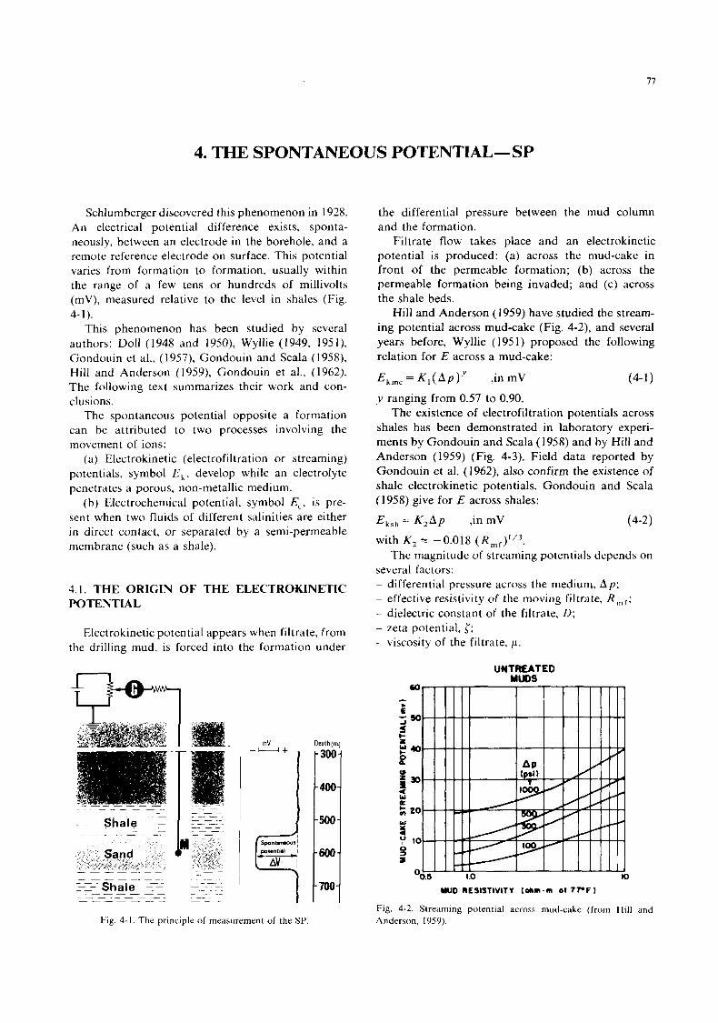
4. THE SPONTANEOUS POTENTIAL- SP
300J
-400-
-500-
-600-
-700-
Schlumberger discovered this phenomenon in 1928. An electrical potential difference exists, sponta- neously, between an electrode in the borehole, and a remote reference electrode on surface. This potential varies from formation to formation, usually within the range of a few tens or hundreds of millivolts (mV), measured relative to the level in shales (Fig.
This phenomenon has been studied by several authors: Doll (1948 and 1950) Wyllie (1949, 1951), Gondouin et al., (1957), Gondouin and Scala (1958), Hill and Anderson ( 1959), Gondouin et al., ( 1 962). The following text summarizes their work and con- clusions.
The spontaneous potential opposite a formation can be attributed to two processes involving the movement of ions:
(a) Electrokinetic (electrofiltration or streaming) potentials, symbol E , , develop while an electrolyte penetrates a porous, non-metallic medium.
(b) Electrochemical potential, symbol E,. is pre- sent when two fluids of different salinities are either in direct contact, or separated by a semi-permeable membrane (such as a shale).
4-1).
4.1. THE ORIGIN OF THE ELECTROKINETIC POTENTIAL
Electrokinetic potential appears when filtrate, from the drilling mud, is forced into the formation under
n _L
I 1 mV --+
Fig. 4-1. The principle of measurement of the SP
Oep I h ( rn)
the differential pressure between the mud column and the formation.
Filtrate flow takes place and an electrokinetic potential is produced: (a) across the mud-cake in front of the permeable formation; (b) across the permeable formation being invaded; and (c) across the shale beds.
Hill and Anderson (1 959) have studied the strearn- ing potential across mud-cake (Fig. 4-2), and several years before, Wyllie ( 1 95 1) proposed the following relation for E across a mud-cake:
Ekmc = K , ( A p ) ’ ,in mV (4-1) y ranging from 0.57 to 0.90.
The existence of electrofiltration potentials across shales has been demonstrated in laboratory experi- ments by Gondouin and Scala (1958) and by Hill and Anderson (1959) (Fig. 4-3). Field data reported by Gondouin et al. ( 1 962), also confirm the existence of shale electrokinetic potentials. Gondouin and Scala (1 958) give for E across shales:
Eksh = K , A p ,in mV (4-2) with K , = -0.018 ( R m r ) 1 / 3 .
several factors: ~ differential pressure across the medium, A p ; ~ effective resistivity of the moving filtrate, R,,,, .; - dielectric constant of the filtrate, D ; - zeta potential, {; - viscosity of the filtrate, p.
The magnitude of streaming potentials depends on
UNTREATED MUDS
MU0 RESISTIVITY (ohm-m O I 7T.F)
Fig. 4-2. Streaming potential across mud-cake (from Hill and Anderson, 1959).
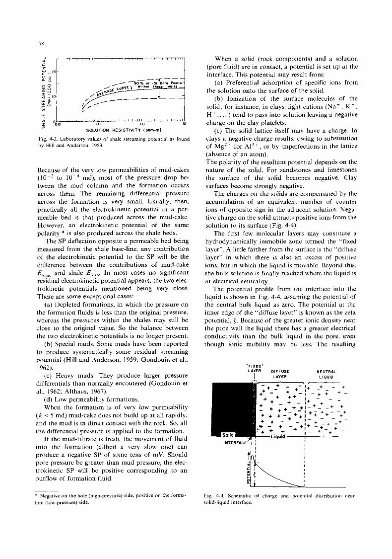
78
I-
$ b-- ?*/
‘1: a L . d 01 10 10 I O0.Ol ul
SOLUTION RESISTIVITY (ohm-m)
Fig. 4-3. Laboratory values of shale streaming potential as found by Hill and Anderson, 1959.
Because of the very low permeabilities of mud-cakes md), most of the pressure drop be-
tween the mud column and the formation occurs across them. The remaining differential pressure across the formation is very small. Usually, then, practically all the electrokinetic potential in a per- meable bed is that produced across the mud-cake. However, an electrokinetic potential of the same polarity * is also produced across the shale beds.
The SP deflection opposite a permeable bed being measured from the shale base-he, any contribution of the electrokinetic potential to the SP will be the difference between the contributions of mud-cake Ekmc and shale Eksh. In most cases no significant residual electrokinetic potential appears, the two elec- trokinetic potentials mentioned being very close. There are some exceptional cases:
(a) Depleted formations, in which the pressure on the formation fluids is less than the original pressure, whereas the pressures within the shales may still be close to the original value. So the balance between the two electrokinetic potentials is no longer present.
(b) Special muds. Some muds have been reported to produce systematically some residual streaming potential (Hill and Anderson, 1959; Gondouin et al., 1962).
(c) Heavy muds. They produce larger pressure differentials than normally encoutered (Gondouin et al., 1962; Althaus, 1967).
to
(d) Low permeability formations. When the formation is of very low permeability
( k < 5 md) mud-cake does not build up at all rapidly, and the mud is in direct contact with the rock. So, all the differential pressure is applied to the formation.
If the mud-filtrate is fresh, the movement of fluid into the formation (allbeit a very slow one) can produce a negative SP of some tens of mV. Should pore pressure be greater than mud pressure, the elec- trokinetic SP will be positive corresponding to an outflow of formation fluid.
* Negative on the hole (high-pressure) side, positive on the forma- tion (low-pressure) side.
When a solid (rock components) and a solution (pore fluid) are in contact, a potential is set up at the interface. This potential may result from:
(a) Preferential adsorption of specific ions from the solution onto the surface of the solid.
(b) Ionization of the surface molecules of the solid; for instance, in clays, light cations @ a + , K + , H t , . . . ) tend to pass into solution leaving a negative charge on the clay platelets.
(c) The solid lattice itself may have a charge. In clays a negative charge results, owing to substitution of Mg2+ for A13+, or by imperfections in the lattice (absence of an atom). The polarity of the resultant potential depends on the nature of the solid. For sandstones and limestones the surface of the solid becomes negative. Clay surfaces become strongly negative.
The charges on the solids are compensated by the accumulation of an equivalent number of counter ions of opposite sign in the adjacent solution. Nega- tive charge on the solid attracts positive ions from the solution to its surface (Fig. 4-4).
The first few molecular layers may constitute a hydrodynamically immobile zone termed the “ fixed layer”. A little farther from the surface is the “diffuse layer” in which there is also an excess of positive ions, but in which the liquid is movable. Beyond this, the bulk solution is finally reached where the liquid is at electrical neutrality.
The potential profile from the interface into the liquid is shown in Fig. 4-4, assuming the potential of the neutral bulk liquid as zero. The potential at the inner edge of the “diffuse layer” is known as the zeta potential, {. Because of the greater ionic density near the pore wall the liquid there has a greater electrical conductivity than the bulk liquid in the pore, even though ionic mobility may be less. The resulting
‘FIXED” LAYER DIFFUSE NEUTRAL
I LAYER LlOUlD
INTERFACEr; I 1
I
Fig. 4-4. Schematic of charge and potential distribution near solid-liquid interface.

19
I 1
I PRESSURE- FLUID FLOW
Fig. 4-5. Generation of electrokinetic potential in a cylindrical pore by application of differential pressure across pore.
increase of conductance across the pore over that expected from the conductivity of the bulk liquid is defined as the surface conductance. It is considered to be relatively independent of pore-water conductiv- Ity.
Figure 4-5 shows how the streaming potential is produced in a cylindrical pore. A differential pressure applied across the pore causes fluid flow through it. Liquid also flows in the diffuse layer carrying along with it its excess positive ions. This movement of charge creates a potential across the length of the pore. This potential results in current flow back through the pore, and a resultant potential drop through the liquid in the pore.
Lynch (1962) proposed the relation:
A
A l
(4-3)
ohm-m p
Fig. 4-6. Example of streaming potential.
where: { D A p is the pressure differential; R , is the water resistivity;
is water viscosity.
is the zeta potential, mentioned above; is the dielectric constant of the water:
Figure 4-6 gives an example of streaming potential appearing in front of a low-permeability formation.
Generally, the electrokinetic potential across the mud-cake is compensated by that across the shale. So one neglects the residual streaming potential and one assumes that the spontaneous potential measured is only related to the electrochemical potential. How- ever, the streaming potential must be recognized be- fore interpreting the SP deflection for R computa- tion. Several features by which one can recognize i t are summarized below:
SP values are abnormally large, resulting in erro- neously low values of R , (compare with RW,;, or known values of R,).
Often SP deflections change quickly with depth giving a “peaky” appearance of the curve.
There may be diminished or no mud-cake, due to low formation permeability (see caliper).
The mud is fresh and formation water is fresh or brackish.
The formation is relatively clean, since shaliness drastically decreases streaming potential (see gamma ray or natural gamma ray spectrometry log).
There must be some porosity (see porosity logs: density, neutron, sonic).
A large differential pressure exists (check mud density). In these cases it is good to have other methods to estimate R,.
4.2. THE ORIGIN OF THE ELECTROCHEMICAL POTENTIAL
The electrochemical potential, Ec, is the sum of two potentials described below.
4.2.1. Membrane potential
An e.m.f. develops when two electrolytes of differ- ent ionic concentrations (mud and formation water) are separated by shale (Figs. 4-7 and 4-9). The clay minerals in shale are made up of lattices of atomic Al, Si, 0 etc. 02- ions occupy the outer extremities, and there is a net negative charge on the lattice. As a result, Na+ ions from solution are attracted and allowed to pass through the shale, while C1- ions are repelled. Na+ ions thus migrate between the two solutions, with a net influx from the more saline to the less. The resulting imbalance of ions on either side of the shale constitutes an e.m.f., the membrane
80
Difference of Dotential
Concentrated NaCl Diluted NaCI
tshale
Fig. 4-7. The membrane potential (after Desbrandes, 1968).
potential (Em).
E m = K , log(aw/amf )
where:
K , = 2.3 R T / F
(the term 2.3 takes care of the conversion from naperian to base- 10 logarithms);
R =ideal gas constant (8.314 joules/"K-mol); T = absolute temperature (in degrees Kelvin); F = Faraday constant (96, 489 coulombs/mol); u, =the ionic activity of the formation water; amf =the ionic activity of the mud filtrate; K , =59.1 mV at 25°C (77°F). For all intents and purposes, Em can be considered constant with time, the actual rate of ionic diffusion being very small (a few mA of current) and the volumes of electrolytes very large. N.B. A small membrane potential also occurs across the mud cake, between the filtrate and the mud. This is usually negligible.
4.2.2. Liquid junction or diffusion potential
This is an e.m.f. established at the contact of the mud filtrate and connate water in an invaded forma- tion (Figs. 4-8 and 4-9). Ions Na+ and C1- have
Difference of potential +m- k a n d
Fig. 4-8. The liquid junction potential (after Desbrandes, 1968).
I ""aded
Zone
Fig. 4-9. The principle of the electrochemical SP. E,. 5 EM + E, .
different mobilities, and therefore do not diffuse at the same rates between the two electrolytes. Na +
tends to be less mobile because of its larger size and an affinity for water molecules. Consequently, a build-up of C1- ions occurs in the weaker solution, and of Nat ions in the more saline solution. This imbalance causes an e.m.f., E,, described by:
= K4 l o g ( a w / a m f 1 (4-6)
The coefficient K , = 11.6 mV at 25°C (77°F). I t is approximated by:
V - u RT K, = 2.3- - v + u F
where: o= mobility of C1 (67.6 x u=mobility of Na (45.6 X
cm2/sV); cm2/sV).
4.2.3. The electrochemical potential, E,
(4-7)
This is the sum of the membrane and liquid junc- tion potentials:
where:
K = K, + K, = 60 + 0.133T (T"F).
E, is arbitrarily defined as zero opposite a shale.
4.3. IONIC ACTIVITY, CONCENTRATION, AND RESISTIVITY
The ionic activity depends on the valency of the cations. Formation waters are usually predominantly solutions of sodium, calcium or magnesium salts. The activity of such a solution is:
(4-9)
81
(PPM,,t PPM,,) or PPMN,
Fig. 4-10. The relationship between ionic activity and concentra- tion (courtesy of Schlumberger).
The chart in Fig. 4-10 can be used to determine the activity from the concentrations. In Fig. 4-1 1 the resistivity of the solution is drawn as a function of ionic activity. Note that it is inversely proportional to the activity below about 80 Kppm total salinity, so that:
(4-10)
At higher concentrations (or more precisely, at higher activities, such as might result from divalent ions), the relationship is more complicated. We simplify the problem by defining equivalent resistivities such that:
(4-1 1)
Equivalent and true resistivities are related as in Fig.
Act iv i ty (Temp 75OF)
v)
& 1.0 c
+!; E r 3
.01 .01 2 3 5 7 .I 2 3 5 7 1 . 0 2 3 5 7 1 0
No+ Activity (Gr-ion / I ) -1 Fig. 4-1 I . The relationship between ionic activity and resistivity (courtesy of Schlumberger).
o w (l,f
7
0 -87
STATIC SP (mi l l ivo l ts1
Fig. 4-12. Determination of R,, from the SP (clean formation) (courtesy of Schlumberger).
4-13. The SP ( E , ) is now a simple logarithmic func- tion of ( R r n f ) J ( R,.,)e as shown in Fig. 4-12.
4.4. THE STATIC SP
In Fig. 4-14a, the spontaneous potential is drawn for the idealized case where no current is allowed to flow in the borehole. The SP is constant across the permeable bed, dropping sharply to zero in the shales (dashed curve). This is the static SP, or SSP, given
r5 r . 2
0
3 1.0 I
2 0.5
- + E E
- k 3 i': I
05 n
- - 2 02
; 01 L
f 005 001 002 005 01 U2 05 01 0 2 R5 10 2
Rmfe or R,, ( at Formation Temperature)
Fig. 4-13. Determination of R , from R,, (courtesy of Schlum- berger).
82
- - - - - - - - - Static SPdiogmm--potential in mud when SP currents are prevented from flowing SP log-potential in mud when SPcurrents are flowing
Fig 4- 14 Schematic representation of potential and current dlstri- bution in dnd around a permeable bed (courtesy of Schlumberger)
by:
(4-12)
The SSP, being defined as zero in the shale, all deflections are measured relative to the SHALE BASE-LINE. Consequently, i t is of the utmost im- portance to correctly define the shale base-line. In reality, a current loop is completed through the mud, and an SP profile similar to that of Fig. 4-14b is produced.
Note that the SP builds up rather gradually from the base-line and that the peak value is less than the SSP. This is referred to as the pseudo-static SP or PSP, and is strongly dependent on bed thickness, the resistivities of the invaded and virgin zones, depth of invasion, shaliness, and so on. These factors also affect the shape of the peak.
4.5. AMPLITUDE AND SHAPE OF S P PEAKS
4.5.1. Hole diameter
The SP is reduced by an increase in hole size, all other factors remaining unchanged.
Fig. 4-15. The effect of invasion on the SP (after Desbrandes. 1968).
4.5.2. Depth of invasion
As Fig. 4-15 shows, the SP decreases as the inva- sion deepens.
4.5.3. Bed thickness
The SP is in fact a measurement of the rise and fall of electrical potential produced by current flow in
1 0 0 m v , 100 mv ~
__ - _ - _ _ -- - --_ __ Permeable Strata
__-._ Stat ic S P D i a g r a m - Fig. 4-16. The effect of bed thickness and resistivity on the shape of the SP (from Doll, 1948).
~- -_ = Impervious Strata
S P Log
83
the mud. Its amplitude approaches the SSP value only when the resistance to current flow offered by the formation and adjacent beds is negligible com- pared with that of the mud (Fig. 4-16). This condition is met only when the bed is thick. So, in general, the SP is reduced in thin beds.
4.5.4. Formation resistivities
The virgin zone-as RJR, increases, the SP deflection decreases-and the bed
No Invasion
' = 5 R Rm
L 0
u) P
n
W \
v) W
1.0
0.0
06
0.4
0.2
R t l R n ,' 40 w 20 In 10 I* S
h/dh
h /dh
less sharply defined (Fig. 4-16). The presence of hydrocarbons therefore attenuates the SP. Neigh- bouring beds-the SP increases with R , / R , ; in- vaded zone- the SP increases with R .JR ,,,.
Charts of the form of Fig. 4-17 are necessary to correct the PSP for these variables, which can have significant effects on the log reading. "SP,,,," in the figure is a good estimate of the PSP. More precise correction charts have been proposed by Segesman
boundaries are ( 1962).
0 0
0 6
04
0 2
40 30 20 I* 10 'S s h /dh
1.0
0 0
0 6
0 4
0 2
I 10
0 0
0 6
0 4
0 2
I .o
0 0
0 6
04
0.2
h/dh @ Schlumberger
I
0
0
0
0.
40 M 20 I* 10 S
h /dh
Fig. 4-17. Correction charts for the SP (courtesy of Schlumberger).
1.0
ao
0.6
0.4
02
40 20 I* 10 '* 5
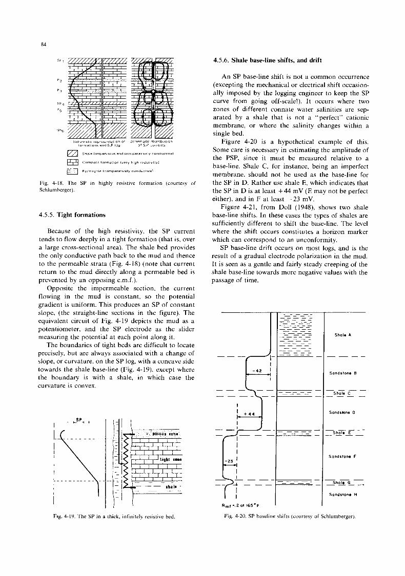
Schematic representation 0 1 Schemaric dlstr lbul lon formations arid S P log O f s P current*
a Shale ( Imper i lour and compararlvely < onducrwel
Compact forrnat8on (very hlgh reslst lwty)
Permeahle ~ComDarat lvelV conducrwe l
Fig 4-18. The SP in highly resistive formation (courtesy of Schlumberger)
4.5.5. Tight formations
Because of the high resistivity, the SP current tends to flow deeply in a tight formation (that is, over a large cross-sectional area). The shale bed provides the only conductive path back to the mud and thence to the permeable strata (Fig. 4-1 8) (note that current return to the mud directly along a permeable bed is prevented by an opposing e.m.f.).
Opposite the impermeable section, the current flowing in the mud is constant, so the potential gradient i s uniform. This produces an SP of constant slope, (the straight-line sections in the figure). The equivalent circuit of Fig. 4-19 depicts the mud as a potentiometer, and the SP electrode as the slider measuring the potential at each point along it.
The boundaries of tight beds are difficult to locate precisely, but are always associated with a change of slope, or curvature, on the SP log, with a concave side towards the shale base-line (Fig. 4- 19), except where the boundary is with a shale, in which case the curvature is convex.
- & + I
I
I I Fig. 4-19. The SP in a thick, infinitely resistive bed.
4.5.6. Shale base-line shifts, and drift
An SP base-line shift is not a common occurrence (excepting the mechanical or electrical shift occasion- ally imposed by the logging engineer to keep the SP curve from going off-scale!). It occurs where two zones of different connate water salinities are sep- arated by a shale that is not a “perfect” cationic membrane, or where the salinity changes within a single bed.
Figure 4-20 is a hypothetical example of this. Some care is necessary in estimating the amplitude of the PSP, since it must be measured relative to a base-line. Shale C, for instance, being an imperfect membrane, should not be used as the base-line for the SP in D. Rather use shale E, which indicates that the SP in D is at least + 44 mV (E may not be perfect either), and in F at least -23 mV.
Figure 4-21, from Doll (1948), shows two shale base-line shifts. In these cases the types of shales are sufficiently different to shift the base-line. The level where the shift occurs constitutes a horizon marker which can correspond to an unconformity.
SP base-line drift occurs on most logs, and is the result of a gradual electrode polarization in the mud. It is seen as a gentle and fairly steady creeping of the shale base-line towards more negative values with the passage of time.
R,f * . 2 01 165-F ’ I
Fig. 4-20. SP baseline shifts (courtesy of Schlumberger).
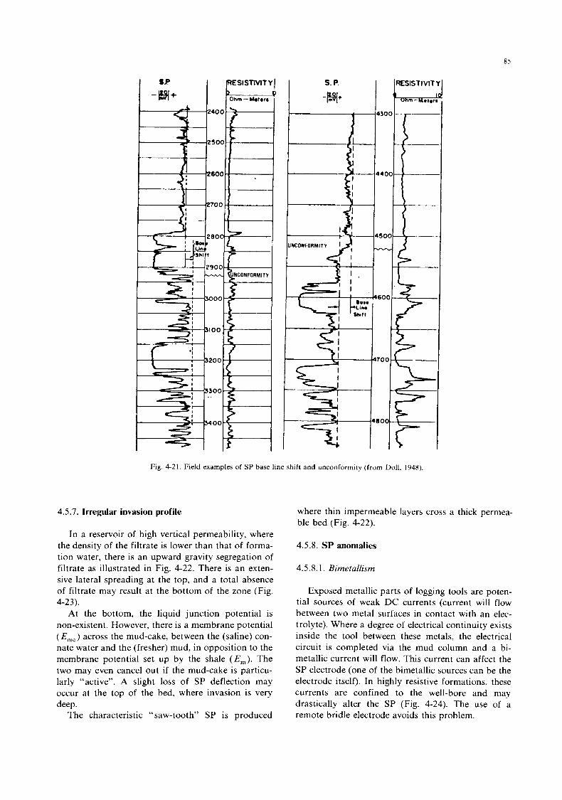
85
Fig. 4-21. Field examples of SP base line shift and unconformity (from Doll, 1948).
4.5.7. Irregular invasion profile
In a reservoir of high vertical permeability, where the density of the filtrate is lower than that of forma- tion water, there is an upward gravity segregation of filtrate as illustrated in Fig. 4-22. There is an exten- sive lateral spreading at the top, and a total absence of filtrate may result at the bottom of the zone (Fig.
At the bottom, the liquid junction potential is non-existent. However, there is a membrane potential ( E m C ) across the mud-cake, between the (saline) con- nate water and the (fresher) mud, in opposition to the membrane potential set up by the shale ( E m ) . The two may even cancel out-if the mud-cake is particu- larly “active”. A slight loss of SP deflection may occur at the top of the bed, where invasion is very deep.
The characteristic “saw-tooth” SP is produced
4-23).
where thin impermeable layers cross a thick permea- ble bed (Fig. 4-22).
4.5.8. SP anomalies
4.5.8.1. Bimetallism
Exposed metallic parts of logging tools are poten- tial sources of weak DC currents (current will flow between two metal surfaces in contact with an elec- trolyte). Where a degree of electrical continuity exists inside the tool between these metals, the electrical circuit is completed via the mud column and a bi- metallic current will flow. This current can affect the SP electrode (one of the bimetallic sources can be the electrode itself). In highly resistive formations, these currents are confined to the well-bore and may drastically alter the SP (Fig. 4-24). The use of a remote bridle electrode avoids this problem.
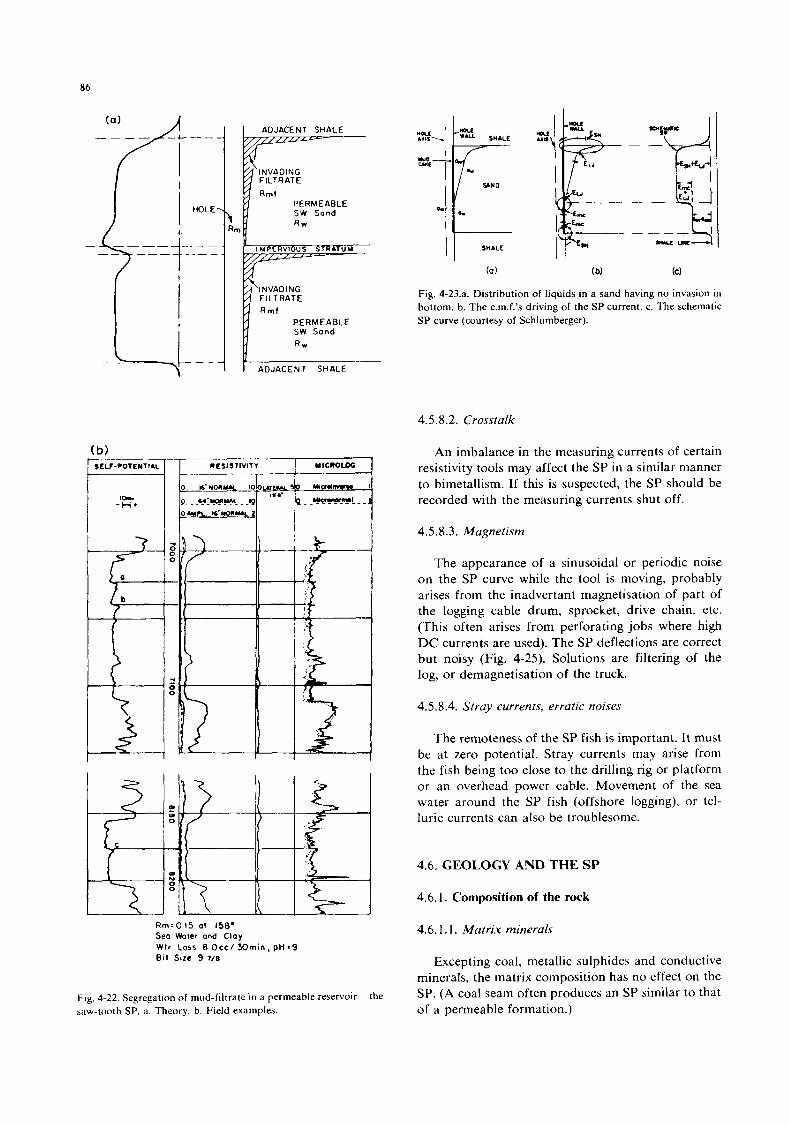
86
I
R m : 0 1 5 at 158’ 520 Woter and Clay W t r Loss 8 O c c / M m i n , pH.9 eat slZc 9 718
Fig. 4-22. Segregation of mud-filtrate in a permeable reservoir-the saw-tooth SP. a. Theory. b. Field examples.
(a 1 (b) (C)
Fig. 4-23.a. Distribution of liquids in a sand having no invasion in bottom. b. The e.m.f.’s driving of the SP current. c. The schematic SP curve (courtesy of Schlumberger).
4.5 3.2. Crosstalk
An imbalance in the measuring currents of certain resistivity tools may affect the SP in a similar manner to bimetallism. If this is suspected, the SP should be recorded with the measuring currents shut off.
4.5.8.3. Magnetism
The appearance of a sinusoidal or periodic noise on the SP curve while the tool is moving, probably arises from the inadvertant magnetisation of part of the logging cable drum, sprocket, drive chain, etc. (This often arises from perforating jobs where high DC currents are used). The SP deflections are correct but noisy (Fig. 4-25). Solutions are filtering of the log, or demagnetisation of the truck.
4.5.8.4. Stray currents, erratic noises
The remoteness of the SP fish is important. It must be at zero potential. Stray currents may arise from the fish being too close to the drilling rig or platform or an overhead power cable. Movement of the sea water around the SP fish (offshore logging), or tel- lurk currents can also be troublesome.
4.6. GEOLOGY AND THE SP
4.6.1. Composition of the rock
4.6.1.1. Matrix minerals
Excepting coal, metallic sulphides and conductive minerals, the matrix composition has no effect on the SP. (A coal seam often produces an SP similar to that of a permeable formation.)
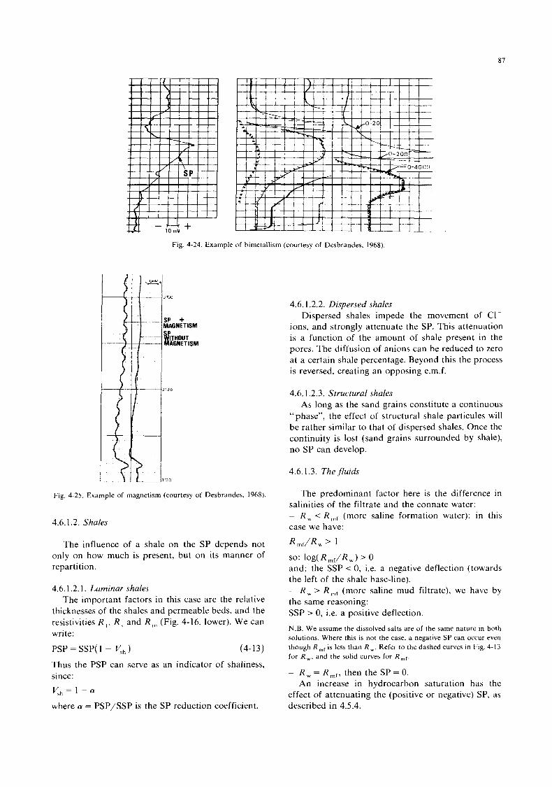
87
Fig 4-24 Example of bimetallism (courtesy of Desbrandes, 1968)
Fig. 4-25. Example of magnetism (courtesy of Desbrandes, 1968)
4.6.1.2. Shales
The influence of a shale on the SP depends not only on how much is present, but on its manner of reparti tion.
4.6.1.2.1. Laminar shales The important factors in this case are the relative
thicknesses of the shales and permeable beds, and the resistivities R , , R , and R , (Fig. 4-16, lower). We can write:
PSP = SSP( 1 - Yh) (4-13)
Thus the PSP can serve as an indicator of shaliness, since: Vlh= 1 - a
where a = PSP/SSP is the SP reduction coefficient.
4.6.1.2.2. Dispersed shales Dispersed shales impede the movement of CI-
ions, and strongly attenuate the SP. This attenuation is a function of the amount of shale present in the pores. The diffusion of anions can be reduced to zero at a certain shale percentage. Beyond this the process is reversed, creating an opposing e.m.f.
4.6.1.2.3. Structural shales As long as the sand grains constitute a continuous
“phase”, the effect of structural shale particules will be rather similar to that of dispersed shales. Once the continuity is lost (sand grains surrounded by shale), no SP can develop.
4.6.1.3. The fluids
The predominant factor here is the difference in
R,, (more saline formation water); in this salinities of the filtrate and the connate water: - R , case we have:
R,r/R, > 1 so: log( R,,/R,) > 0 and: the SSP < 0, i.e. a negative deflection (towards the left of the shale base-line). - R , > Rn,r (more saline mud filtrate), we have by the same reasoning: SSP > 0, i.e. a positive deflection. N.B. We assume the dissolved salts are of the same nature in both solutions. Where this is not the case. a negative SP can occur even though R,, is less than R, . Refer to the dashed curves in Fig. 4-13 for R , , and the solid curves for R,,,,.
- R , = R m f , then the SP = 0. ~ An increase in hydrocarbon saturation has the effect of attenuating the (positive or negative) SP, as described in 4.5.4.
88
4.6.2. Rock texture 4.8. REFERENCES
There is no known direct correlation between per- meability, porosity, and the amplitude of the SP. Certainly, both must be present for an SP to develop, and in that they influence invasion (4.5.2.) and fluid segregation (4.5.7), we can say that the sedimentology of the formation is one of the factors affecting the SP.
Shale distribution is discussed in 4.6.1.2.
4.6.3. Temperature
K is temperature-dependent, and is approximated
(4-14) by: K = 60 + 0.133T ( O F )
4.6.4. Pressure
The pressure difference between the well-bore and the formation influences: (a) the diameter of inva- sion; and (b) a possible electrokinetic SP.
4.6.5. Depositional environment, sequential evolution
These factors determine the bed thicknesses, and for a given bed, the nature of its “environment”, i.e. its adjacent (4.5.3 and 4.5.4).
The actual shape of the SP curve (Shell geologists have devised a classification including bell-, funnel- and egg-shaped, etc.) depends on the sequential evolution within the bed, since this will manifest itself as an “evolution” of spontaneous potential (upward coarsening, upward fining, and so on).
4.7. APPLICATIONS
(a) Identification of porous, permeable beds (pro-
(b) Determination of R, . (c) A lithological indicator: shales, coal-seams,
(d) An analysis of the facies and grading, based on
(e) Correlation. (f) An indication of possible hydrocarbon satura-
tion in shaly sands, including the presence of a gas-oil contact. These applications will be discussed in volume 2 .
vided the other conditions discussed are met).
shale fraction estimation from: Kh < 1 - PSP/SSP.
the curve shape.
Althaus, V.E., 1967. Electrokinetic potentials in South Louisiana
Chombart, L.G., 1957. Reconnaissance d’evaluation des forrna-
Dickey, P.A., 1944. Natural potentials in sedimentary rocks. Trans.
Doll, H.G., 1948. The S.P. Log: theoretical analysis and principles
Doll, H.G., 1950. The S.P. log in shaly sands. Trans. AIME. 189. Gondouin, M. and Scala, C., 1958. Streaming potential and the
S.P. log. J. Pet. Technol., 10 (8). Gondouin, M., Tixier, M.P. and Simard, G.L. (1957). An experi-
mental study on the influence of the chemical compositlon of electrolytes on the S.P. curve. J. Pet. Technol., 9 (2).
Gondouin, M., Hill, H.J. and Waxman. M.H., 1962. A field streaming potential experiment. J. Pet. Technol., 14 (3).
Hill, H.J. and Anderson, A.E., 1959. Streaming potential phenom- ena in S.P. log interpretation. Trans. AIME. 216.
Kerver, J.K. and Prokop, C.L., 1957. Effect of the presence of hydrocarbons on well logging potential. Soc. Petrol. Eng. of AIME, Los Angeles Meeting, October 1957.
Lynch, E.J., 1962. Formation Evaluation. Harper’s Geoscience Series, Harper and Row, New-York.
McCardell, W.M.. Winsauer, E.O. and Williams, M., 1953. Origin of the electric potential observed in wells. J. Pet. Technol., 5
Mallenburg, J.K., 1973. Interpretation of gamma ray logs. The Log Analyst, 14(6).
Mounce, W.D. and Rust, W.M., Jr.. 1943. Natural potentials in well logging. J. Pet. Technol., 6.
Pied, B. and Poupon. A., 1966. SP base-line shift in Algeria. 7th Ann. Symp. S.P.W.L.A.
Pirson. S.J. (1947) A study of the self potential curve. Oil Gas J. Oct. 4.
Poupon, A. and Lebreton, F. Diagraphies nucleaires. Inst. f r a y . Petr. ENSPM, ref. 2432.
Schlumberger, C.M. Schlumberger, C. and Leonardon, E.G.. 1934. A new contribution to subsurface studies by means of electrical measurements in drill holes. Trans. AIME. 110.
Segesman, F., 1962. New SP correction charts. Geophysics, vol. 27, n 6, part I .
Segesman, F. and Tixier, M.P., 1959. Some effects of invasion on the S.P. curve. Trans. AIME, 216.
White, C.C., 1946. A study of the self potential curve. Oil Gas. J.. 14 Dec.
Witte, L. de 1950. Experimental studies on the characteristics of the electrochemical potential encountered in drill holes. AIME, Los Angeles, 12-13 October 1950.
Worthington, A.E. and Meldau, R.F., 1958. Departure curves for the self-potential log. J. Pet. Technol., 10 ( I ) .
Wyllie, M.R.J., 1949. A quantitative analysis of the electrochemical component of the S.P. curve. J. Pet. Technol., 1 ( I ) .
Wyllie, M.R.J., 195 1. An investigation of the electrokinetic compo- nent of the S.P. curve. J. Pet. Technol., 3 (1).
Wyllie, M.R.J., Witte, A.J. de, and Warren, J.E., 1958. On the streaming potential. Trans. AIME, 213.
Tertiary sediments. The Log Analyst, 8 ( I ) .
tions par diagraphies electriques et nucleaires. Technip, Paris.
AIME, 155.
of interpretation. Trans. AIME. 179 ( 1 1 ) .
(3).
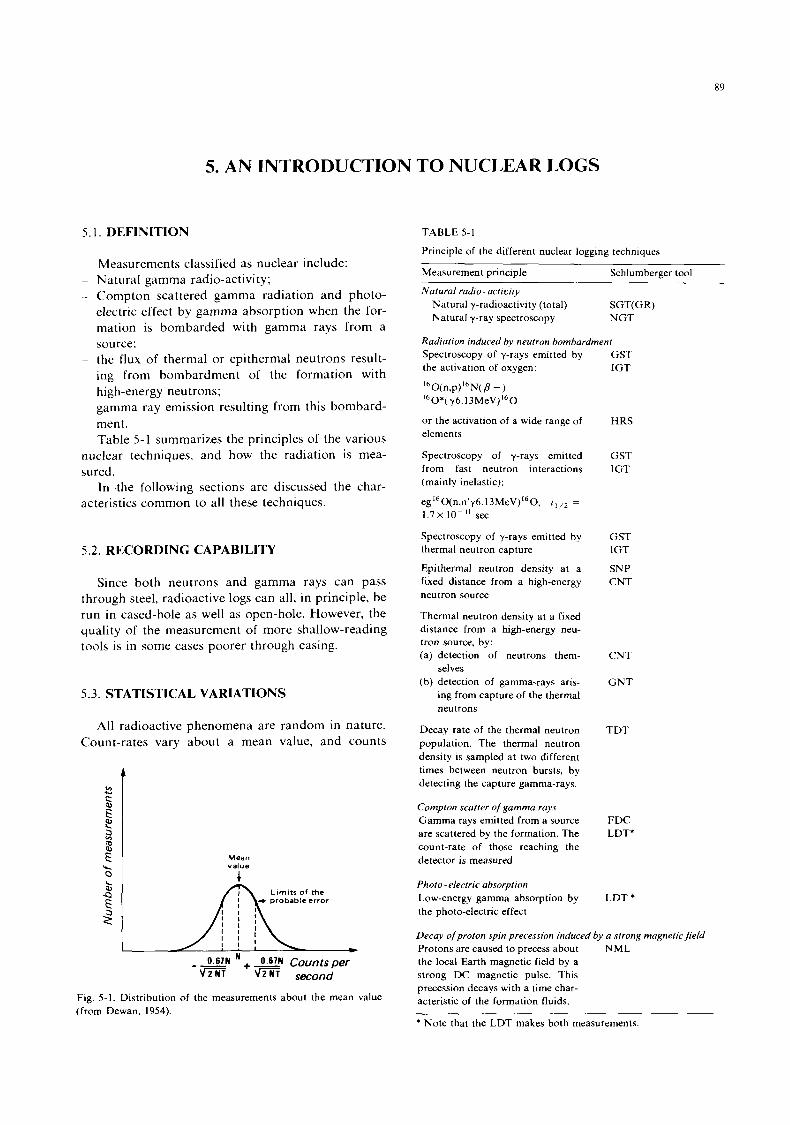
R9
5. AN INTRODUCTION TO NUCLEAR LOGS
5.1. DEFINITION
Measurements classified as nuclear include: ~ Natural gamma radio-activity; - Compton scattered gamma radiation and photo-
electric effect by gamma absorption when the for- mation is bombarded with gamma rays from a source;
- the flux of thermal or epithermal neutrons result- ing from bombardment of the formation with high-energy neutrons;
~ gamma ray emission resulting from this bombard- ment. Table 5- 1 summarizes the principles of the various
nuclear techniques, and how the radiation is mea- sured.
In .the following sections are discussed the char- acteristics common to all these techniques.
5.2. RECORDING CAPABILITY
Since both neutrons and gamma rays can pass through steel, radioactive logs can all, in principle, be run in cased-hole as well as open-hole. However, the quality of the measurement of more shallow-reading tools is in some cases poorer through casing.
5.3. STATISTICAL VARIATIONS
All radioactive phenomena are random in nature. Count-rates vary about a mean value, and counts
j[ e, F
Mean value
Fig. 5-1. Distribution of the measurements about the mean value (from Dewan, 1954).
TABLE 5-1
Principle of the different nuclear logging techniques
Measurement principle Schlumberger tool
Natural radio - activity Natural y-radioactivity (total) SGT(GR) Natural y-ray spectroscopy NGT
Radiation induced by neutron bombardment Spectroscopy of y-rays emitted by GST the activation of oxygen: IGT
160(n,p)'6N(P - ) I6O*( y6.I3MeV)I60
or the activation of a wide range of elements
Spectroscopy of y-rays emitted GST from fast neutron interactions IGT (mainly inelastic):
eg160(n,n'y6. 1 3MeV)I60, 1.7X10-" sec
Spectroscopy of y-rays emitted by GST thermal neutron capture IGT
Epithermal neutron density at a SNP fixed distance from a high-energy CNT neutron source
Thermal neutron density at a fixed distance from a high-energy neu- tron source, by: (a) detection of neutrons them- CNT
selves (b) detection of gamma-rays aris- GNT
ing from capture of the thermal neutrons
HRS
t I,z =
Decay rate of the thermal neutron population. The thermal neutron density is sampled at two different times between neutron bursts, by detecting the capture gamma-rays.
Compton scatter of gamma rays Gamma rays emitted from a source are scattered by the formation. The count-rate of those reaching the detector is measured.
Photo - electric absorption Low-energy gamma absorption by the photo-electric effect
Decay of proton spin precession induced by a strong magnetic field Protons are caused to precess about the local Earth magnetic field by a strong DC magnetic pulse. This precession decays with a time char- acteristic of the formation fluids.
TDT
FDC LDT*
LDT *
NML
* Note that the LDT makes both measurements.
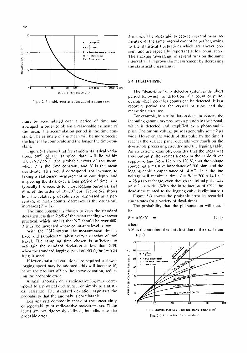
90
U 0 0: U W
20 31
COUNTS PER SECOND (N)
Fig. 5-2. Propable error as a function of a count-rate.
must be accumulated over a period of time and averaged in order to obtain a reasonable estimate of the mean. The accumulation period is the time con- stant. The estimate of the mean will be more precise the higher the count-rate and the longer the time-con- stant.
Figure 5- 1 shows that for random statistical varia- tions. 50% of the sampled data will lie within * 0 . 6 7 N / d 2 P f (the probable error) of the mean, where T is the time constant, and N is the mean count-rate. This would correspond, for instance, to taking a stationary measurement at one depth, and inspecting the data over a long period of time. T is typically 1-6 seconds for most logging purposes, and N is of the order of 10-10’ cps. Figure 5-2 shows how the relative probable error, expressed as a per- centage of mean counts, decreases as the count-rate increases ( T = ts).
The time constant is chosen to keep the standard deviation less than 2.5% of the mean reading wherever practical, which implies that NT should be over 400. T must be increased where count-rate level is low.
With the CSU system, the measurement time is fixed and samples are taken every six inches of tool travel. The sampling time chosen is sufficient to maintain the standard deviation at less than 2.5% when the standard logging speed of 900 ft/hr ( = 0.25 ft/s) is used.
If lower statistical variations are required, a slower logging speed may be adopted; this will increase N , hence the product N T in the above equation, reduc- ing the probable error.
A small anomaly on a radioactive log may corre- spond to a physical occurrence, or simply to statisti- cal variation. The standard deviation expresses the probability that the anomaly is correlatable.
Log analysts commonly speak of the uncertainty or repeatability of radio-active measurements. These terms are not rigorously defined, but allude to the probable error.
Remarks. The repeatability between several measure- ments over the same interval cannot be perfect. owing to the statistical fluctuations which are always pre- sent, and are especially important at low count rates. The stacking (averaging) of several runs on the same interval will improve the measurement by decreasing the statistical uncertainty.
5.4. DEAD-TIME
The “dead-time’’ of a detector system is the short period following the detection of a count or pulse, during which no other counts can be detected. I t is a recovery period for the crystal or tube, and the measuring circuitry.
For example, in a scintillation detector system, the incoming gamma ray produces a photon in the crystal, which is detected and amplified by a photo-multi- plier. The output voltage pulse is generally some 2 ps wide. However, the width of this pulse by the time i t reaches the surface panel depends very much on the down-hole processing circuitry and the logging cable. As an extreme example, consider that the (negative) P-M output pulse creates a drop in the cable driver supply voltage from 125 V to 120 V, that the voltage source has a resistive impedance of 200 ohm, and the logging cable a capacitance of 14 pF. Then the line voltage will require a time T = RC = 200 X 14.10-‘ = 28 ps to recharge, even though the initial pulse was only 2 ps wide. (With the introduction of CSU the dead-time related to the logging cable is eliminated.)
Figure 5-3 shows the probable error in recorded count-rates for a variety of dead-times.
The probability that the phenomenon will occur is: P = A N / N = nt (5-1) where: A N is the number of counts lost due to the dead-time
(CPS> I I I / I 1
0 20 40 60 80 100
TRUE COUNTS PER SEC IFOR NIL DEAD-TIME) x lo3
Fig. 5-3. Correction for dead-time.
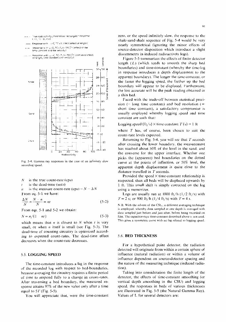
91
- _ -
__
. . . . . . . ..
True radioactlvlty, theoretical rectangular response zero. or the speed infinitely slow, the response t o the shale-sand-shale sequence of Fig. 5-4 would be very nearly symmetrical (ignoring the minor effects of source-detector disposition which introduce a slight dissymmetry in induced radioactivity logs).
length ( L ) (which tends to smooth the sharp bed
L = 0, TC z 0, V = O
Response with L: 4', TC =O, V # O (effect of length)
Response with L:O,TCz7,V=720yh (effect Of the tlme constant and the velocity)
Response wlth L24: TC.7, V=720'/h (combined effect in n Figure 5-5 summarizes the effects of finite detector 01 length, t ime constant and VeIOclty)
z e a ' a '
Shale
Sand
Shale
0 20*60 80 100
I 32- 160
28-140 c
E 24-120 -
a VI
U 20-100 $ s 16- 80
12- 60
8- 40
4 - 20
0- 0
- 4 - - 2 0
- 8 - - 4 0
Radioac t IV i t y
Fig. 5-4. Gamma ray responses in the case of an infinitely slow recording speed.
N t is the dead-time (secs) n
From eq. 5-1 we have: A N N - n N N
is the true count-rate (cps)
is the measure count-rate (cps) = N - A N
nt ~ - _ _ _ = - ( 5 - 2 )
From eqs. 5-1 and 5-2 we obtain:
N = n / ( l - n t ) ( 5 - 3 )
which means that n is closest to N when t is very small, or when n itself is small (see Fig. 5-3). The dead-time of counting circuitry is optimized accord- ing to expected count-rates. The dead-time effect decreases when the count-rate decreases.
5.5. LOGGING SPEED
The time-constant introduces a lag in the response o f the recorded log with respect to bed-boundaries, because averaging the circuitry requires a finite period of time to respond fully to a change in count-rates. After traversing a bed boundary, the measured re- sponse attains 97% of the new value only after a time equal to 5 T (Fig. 5-5) .
You will appreciate that, were the time-constant
boundaries) and time-constant (whereby the time-log in response introduces a depth displacement to the apparent boundary). The longer the time-constant, or the faster the logging speed, the farther up the bed boundary will appear to be displaced. Furthermore, the less accurate will be the peak reading obtained in a thin bed.
Faced with the trade-off between statistical preci- sion (= long time constant) and bed resolution ( =
short time constant), a satisfactory compromise is usually employed whereby logging speed and time constant are such that:
Logging speed (ft/s) X time constant T ( s ) = 1 f t
where T has, of course, been chosen to suit the count-rate levels expected.
Returning to Fig. 5-4, you will see that T seconds after crossing the lower boundary, the measurement has reached about 50% of the level in the sand, and the converse for the upper interface. Whether one picks the (apparent) bed boundaries on the dotted curve at the points of inflection, or 50% level, the apparent depth displacement is quite close to the distance travelled in T seconds.
Provided the speed x time-constant relationship is respected, than all beds will be displaced upwards by 1 ft. This small shift is simply corrected on the log using a memorizer.
Logs are usually run at 1800 ft/h (1/2 ft/s) with T = 2 s; or 900 ft/h (1/4 ft/s) with T = 4 s.
N.B. With the advent of the CSU, a different averaging technique is employed. whereby data sampled at one depth is averaged with data sampled just before and just after. before being recorded on film. The capacitor-type time-constant described above is not used. This gives a symmetric curve with no lag related to logging speed.
5.6. BED THICKNESS
For a hypothetical point detector, the radiation detected will originate from within a certain sphere of influence (natural radiation) or within a volume of influence dependent on source-detector spacing and the nature of the measuring technique (induced radia- tion).
Taking into consideration the finite length of the detector, the effects of time-constant smoothing (or vertical depth smoothing in the CSU) and logging speed, the responses in beds of various thicknesses are illustrated in Fig. 5-5 (the Natural Gamma Ray). Values of L for several detectors are:
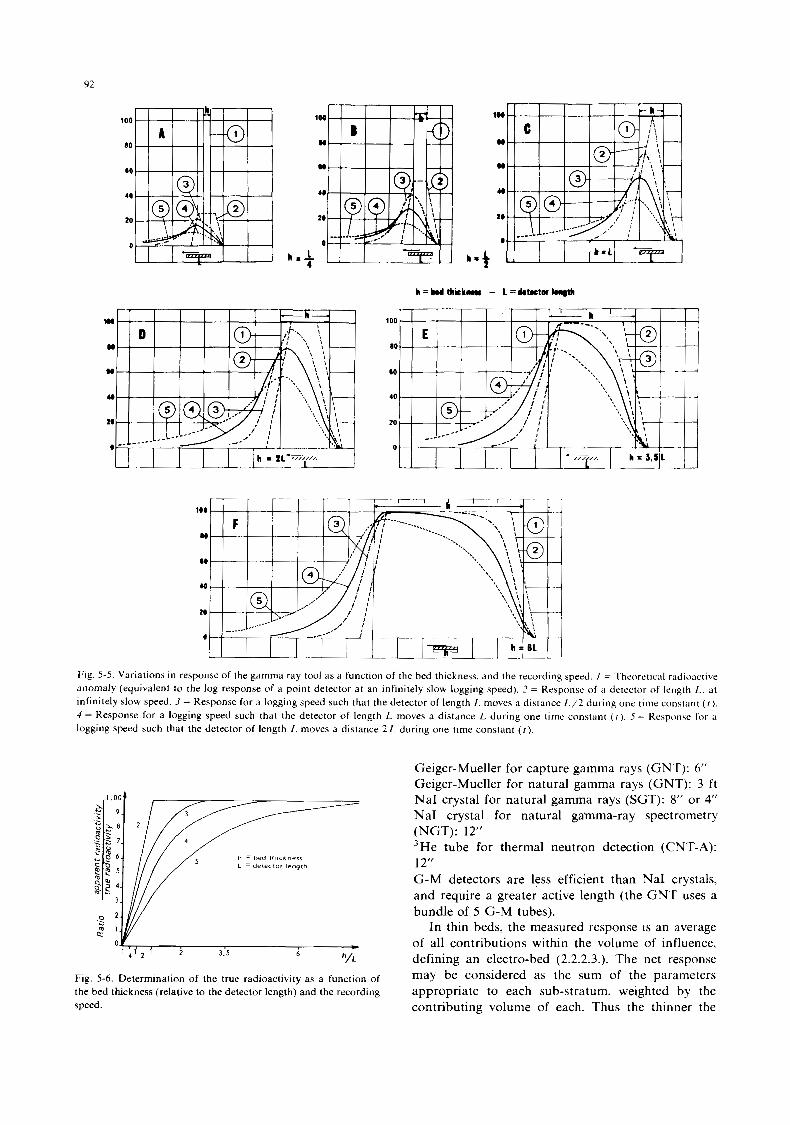
92
100
80
00
40
20
o - , i r w I c
h . 1 4
loo
n
20
0
100
80
60
40
20
0
Fig. 5 5 . Variations in response of the gamma ray tool as a function of the bed thickness. and the recording speed. I = Theoretical radioactive anomaly (equivalent to the log response of a point detector at an infinitely slow logging speed). 2 = Response o f il detector o f length L . at infinitely slow speed. 3 = Response for a logging speed such that the detector of length L moves a distance L / 2 during one time constant ( I ) .
4 = Response for a logging speed such that the detector of length L moves a distance L during one time constant ( I ) . 5 = Response for il logging speed such that the detector of length L moves a distance 2 L during one time constant ( t ) .
Geiger-Mueller for capture gamma rays (GNT): 6” Geiger-Mueller for natural gamma rays (GNT): 3 f t NaI crystal for natural gamma rays (SGT): 8” or 4” NaI crystal for natural gamma-ray spectrometry (NGT): 12” 3He tube for thermal neutron detection (CNT-A): 12“ G-M detectors are less efficient than NaI crystals, and require a greater active length (the GNT uses a bundle of 5 G-M tubes).
In thin beds, the measured response IS an average of all contributions within the volume of influence, defining an electro-bed (2.2.2.3.). The net response may be considered as the sum Of the parameters appropriate to each sub-stratum, weighted by the contributing volume of each. Thus the thinner the
h = b e d thickness L = detector length
- 2 6
h/L ’ 4 ’ 2 ‘ 3.5
Fig. 5-6. Determination of the true radioactivity as a function of the bed thickness (relative to the detector length) and the recording speed.
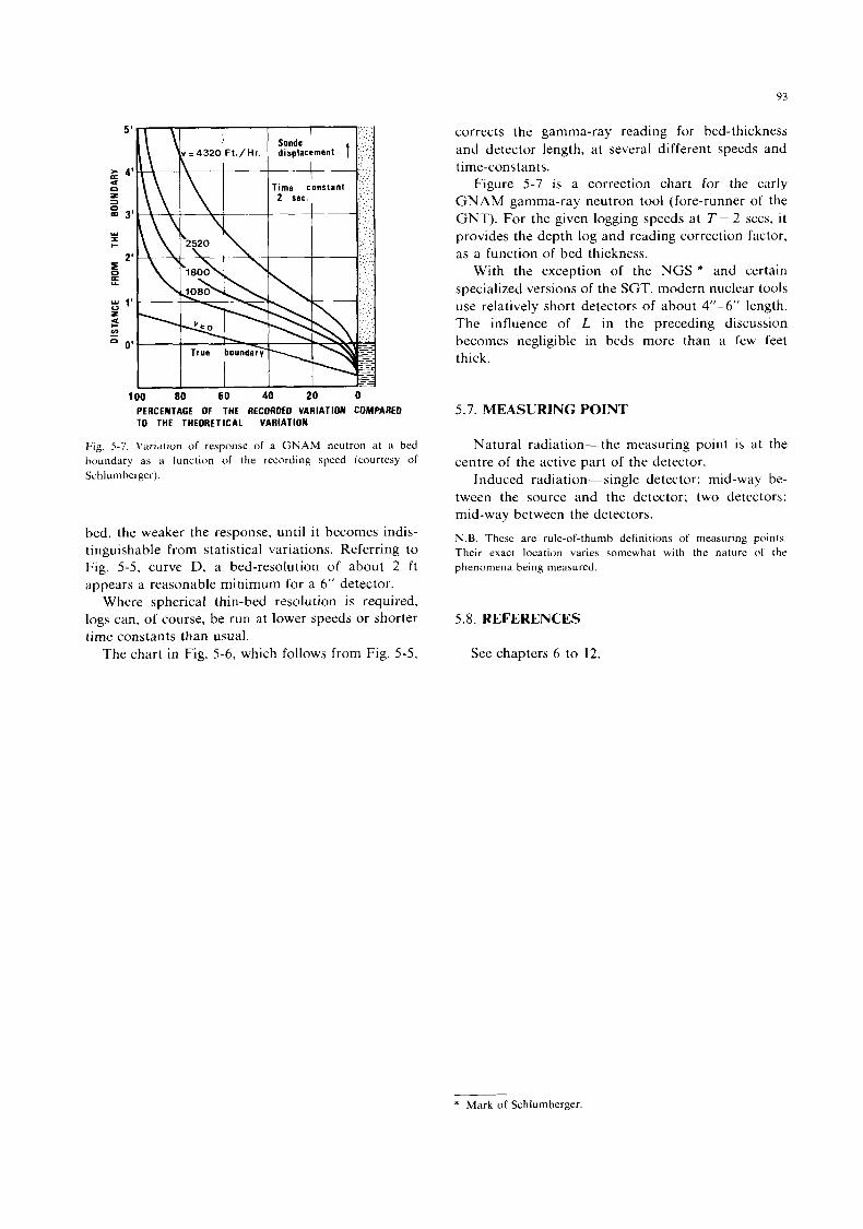
93
corrects the gamma-ray reading for bed-thickness and detector length, at several different speeds and time-constants.
Figure 5-7 is a correction chart for the early GNAM gamma-ray neutron tool (fore-runner of the GNT). For the given logging speeds at T = 2 secs, i t provides the depth log and reading correction factor, as a function of bed thickness.
With the exception of the NGS * and certain specialized versions of the SGT, modern nuclear tools use relatively short detectors of about 4”-6” length. The influence of L in the preceding discussion becomes negligible in beds more than a few feet thick.
100 80 60 40 20 0 PERCENTAGE OF THE RECORDEO VARIATION COMPARED TO THE THEORETICAL VARIATION
Flg. 5-7. Variation o f response of a GNAM neutron at a bed boundary as a function of the recording speed (courtesy of Schlumberger).
bed, the weaker the response, until i t becomes indis- tinguishable from statistical variations. Referring to Fig. 5-5, curve D, a bed-resolution of about 2 f t appears a reasonable minimum for a 6” detector.
Where spherical thin-bed resolution is required, logs can, of course, be run at lower speeds or shorter time constants than usual.
The chart in Fig. 5-6, which follows from Fig. 5-5,
5.7. MEASURING POINT
Natural radiation-the measuring point is at the centre of the active part of the detector.
Induced radiation-single detector: mid-way be- tween the source and the detector; two detectors: mid-way between the detectors. N.B. These are rule-of-thumb definitions of measuring points. Their exact location varies somewhat with the nature of the phenomena being measured.
5.8. REFERENCES
See chapters 6 to 12.
~~
* Mark of Schlumberger

This Page Intentionally Left Blank
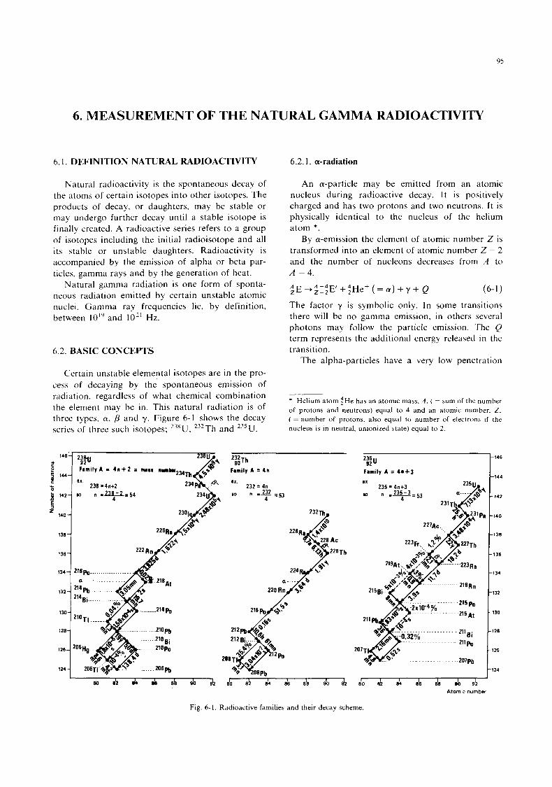
95
6. MEASUREMENT OF THE NATURAL GAMMA RADIOACTIVITY
6.1. DEFINITION NATURAL RADIOACTIVITY
Natural radioactivity is the spontaneous decay of the atoms of certain isotopes into other isotopes. The products of decay, or daughters, may be stable or may undergo further decay until a stable isotope is finally created. A radioactive series refers to a group o f isotopes including the initial radioisotope and all its stable or unstable daughters. Radioactivity is accompanied by the emission of alpha or beta par- ticles, gamma rays and by the generation of heat.
Natural gamma radiation is one form of sponta- neous radiation emitted by certain unstable atomic nuclei. Gamma ray frequencies lie, by definition, between 10" and 10" Hz.
6.2. BASIC CONCEPTS
Certain unstable elemental isotopes are in the pro- cess of decaying by the' spontaneous emission of radiation, regardless of what chemical combination the element may be in. This natural radiation is of three types, a, p and y. Figure 6-1 shows the decay series o f three such isotopes; 23xU, 232Th and 235U.
138 1
6.2.1. a-radiation
An &-particle may be emitted from an atomic nucleus during radioactive decay. I t is positively charged and has two protons and two neutrons. It is physically identical to the nucleus of the helium atom *.
By a-emission the element of atomic number Z is transformed into an element of atomic number Z - 2 and the number of nucleons decreases from A to A - 4.
$E+$I ;E +;He+ ( = a ) + y + Q (6-1) The factor y is symbolic only. In some transitions there will be no gamma emission, in others several photons may follow the particle emission. The Q term represents the additional energy released in the transition.
The alpha-particles have a very low penetration
* Helium atom :He has an atomic mass, A . ( = sum o f the number of protons and neutrons) equal to 4 and an atomic numher. Z . ( = number of protons. also equal to number of electrons if the nucleus is In neutral, unionized state) equal to 2.
232
Family A = 4n
232 = 4n so n ,232 =53
4
90Th
ex
216 h/
235 92
Family A = 4 0 + 3
I I 8 0 e!? M 8b ds do 9h
Atomic number
-I46
-144
. I42
140
138
136
134
132
130
I28
I26
I24
Fig. 6-1. Radioactive families and their decay scheme.
96
TABLE 6-1
Penetration o f a-particles in different materiala as a function of their energy
Energy of a- 1 2 3 4 5 6 7 Particles (MeV)
Air (mm) 5 10 17 25 35 47 59 Aluminium(pni) 4 7 1 1 16 22 29 Iron (pni ) 2 4 6 8 1 1 14 Water. paper 10 19 29 41 54 71 Plastic ( p m )
power and at normal temperature and pressure can only penetrate most materials to only a few tens of p m (Table 6-1).
6.2.2. P-radiation, P + or P
A ,&particle may be emitted from an atomic nucleus during radioactive decay. I t is physically identical to the electron. It may be either positively charged (positron) or negatively charged (electron).
During p- -emission the element of atomic num- ber Z becomes the element of atomic number Z + 1.
/ E +7+ ,E’ + ,l- + n o + y + Q (6-2) y and Q as above, n o represents the neutrino.
During p’-emission the element of atomic num- ber Z becomes the element of atomic number Z - 1. ,E +7- ,E’ + p’ + n o + y + Q (6-3) ,&particles have a higher penetration power than a. It d e p e n d s o n t h e kinet ic energy of the electron/positron. For instance, at 1 MeV energy, penetration is about 4 m in air, and 2 mm in aluminium (Table 6-2).
Like a-radiation, &radiation is generally too weak to be of direct interest as a logging measurement.
6.2.3. y-radiation
y-radiation may be considered as an electromag- netic wave similar to visible light or X-rays, or as a
particle or photon. Gamma rays are electromagnetic radiations emitted from an atomic nucleus during radioactive decay. These radiations are characterized by wave lengths in the range of 1 0 ~ ’ - 1 0 ~ ” cm, equivalent to frequencies ranging from 10’’ to 10” sec I.
The gamma-emission corresponds, in a nucleus, to the transition from one state to another of lower energy with emission of a photon of energy hv, equal to the difference between the energies of the two states. The energy is related to the wavelength, A , or frequency v, by:
E = hv = hc/X (6-4)
where c is the velocity of light, and h is Planck’s constant (6.626 x lop2’ erg s or 6.626 X joule s).
The energy is expressed in electron-volts (eV) *. The energies of gamma rays are of the order of the KeV (10’ eV) or the MeV ( lo6 eV).
Usually, the a-, p- and y-emissions are simulta- neous. a- and /?-particles do not penetrate far enough to be detected by logging techniques. The gamma rays have a very high power of penetration (Table 6-3) and can be detected and recorded in present-day hole condictions. For that reason, they are the basis of several important logging techniques.
6.2.4. Radioactive decay
The decay or disintegration of an atom involves the emission of a , j3, or y radiations, and heat, resulting in the transformation of that atom into another, lower down the decay series (Fig. 6-1). The final atomic state at the end of the series is stable. The radioactive decay is a pure statistical process. At a
* One electron-volt is the energy acquired by a charged particle carrying unit electronic charge when i t is accelerated by a potential difference of one volt. One eV is equivalent to 1.602 x 10- ’’ erg or 1 . 6 0 2 ~ joule. One eV is associated through the Planck constant with a photon of wavelength 1.239 pm. For an energy of 1 MeV. the wave-length is equal to 0.0124 A.
TABLE 6-2
Penetration of electrons in different materials as a function of their energy (all values in mm)
Energy in Mev 0.01 0.03 0.1 0.3 0.7 Material (density)
Air (0.001 3) 1.9 15 120 730 2440 Water ( 1 .O) 0.002 0.0 17 0.14 0.8 2.7 Vinyl polychloride 0.002 0.015 0.12 0.74 2.4 Hexiglass ( 1.19) 0.002 0.014 0.12 0.71 2.4 Aluminium (2.7) 0.001 0.009 0.07 0.40 1.3 Iron (7.8) o . 4 ~ 3 . 4 ~ I O - ~ 0.027 0.16 0.50 Lead ( 1 1.35) 0 . 5 2 ~ lo-) 3 . 7 ~ I O - ~ 0.028 0.14 0.44
1
3 800 4.3 3.8 3.7 2.1 0.78 0.67
2 3
8 350 12800 9.6 14.9 8.5 13.1 8.4 13.1 4.5 6.9 1.7 2.6 1.4 2. I
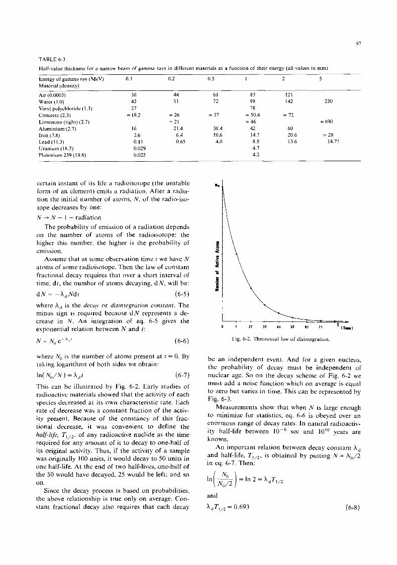
97
TABLE 6-3
Half-value thickness for a narrow beam of gamma rays in different materials as a function of their energy (all values in mm)
Energy of gamma ray (MeV) 0.1 0.2 0.5 1 2 5 Material (density)
Air (0.0003) Water ( 1 .O) Vinyl polychloride (1.3) Concrete (2.3) Limestone (tight) (2.7) Aluminium (2.7) Iron (7.8) Lead ( 1 1.3) Uranium (18.7) Plutonium 239 (19.8)
36 44 42 51 27
= 19.2 = 26 = 21
16 21.4 2.6 6.4 0.1 1 0.65 0.029 0.025
61 83 121 72 98 142 230
78 = 37 = 50.4 = 72
= 46 = 100 30.4 42 60 10.6 14.7 20.6 = 28 4.0 8.8 13.6 14.7?
4.7 4.2
certain instant of its life a radioisotope (the unstable form of an element) emits a radiation. After a radia- tion the initial number of atoms, N, of the radio-iso- tope decreases by one: N + N - 1 + radiation
The probability of emission of a radiation depends on the number of atoms of the radioisotope: the higher this number, the higher is the probability of emission.
Assume that at some observation time t we have N atoms of some radioisotope. Then the law of constant fractional decay requires that over a short interval of time, dt , the number of atoms decaying, dN, will be:
d N = -A,Ndt (6-5) where A, is the decay or disintegration constant. The minus sign is required because d N represents a de- crease in N. An integration of eq. 6-5 gives the exponential relation between N and t:
where 4, is the number of atoms present at t = 0. By taking logarithms of both sides we obtain:
In( N,,," ) = A,t (6-7) This can be illustrated by Fig. 6-2. Early studies of radioactive materials showed that the activity of each species decreased at its own characteristic rate. Each rate of decrease was a constant fraction of the activ- ity present. Because of the constancy of this frac- tional decrease, it was convenient to define the half-life, TI , , , of any radioactive nuclide as the time required for any amount of it to decay to one-half of its original activity. Thus, if the activity of a sample was originally 100 units, i t would decay to 50 units in one half-life. At the end of two half-lives, one-half of the 50 would have decayed, 25 would be left; and so on.
Since the decay process is based on probabilities, the above relationship is true only on average. Con- stant fractional decay also requires that each decay
' (Tim) 0 T 2T 31 4 1 5 1 6 1 7 1
Fig. 6-2. Theoretical law of disintegration.
be an independent event. And for a given nucleus, the probability of decay must be independent of nuclear age. So on the decay scheme of Fig. 6-2 we must add a noise function which on average is equal to zero but varies in time. This can be represented by Fig. 6-3.
Measurements show that when N is large enough to minimize for statistics, eq. 6-6 is obeyed over an enormous range of decay rates. In natural radioactiv- ity half-life between sec and 10" years are known.
An important relation between decay constant A, and half-life, Ti,,, is obtained by putting N = N0/2 in eq. 6-7. Then:
and
AdTi,2 = 0.693
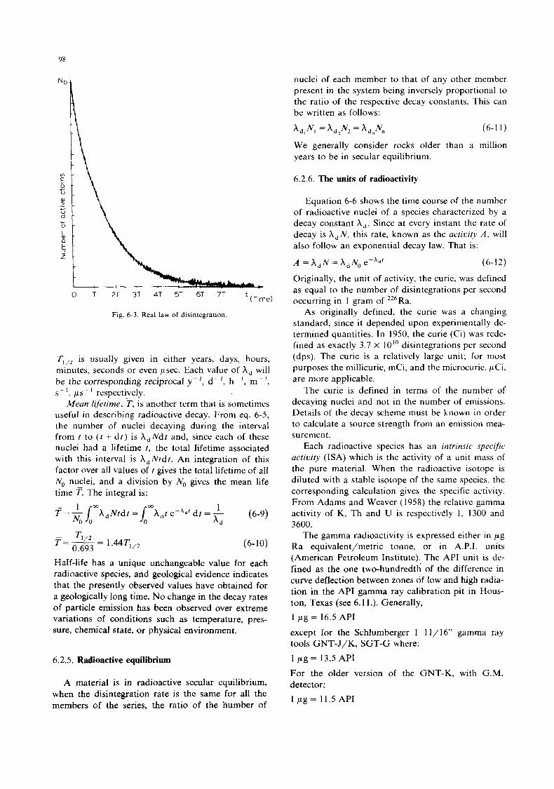
98
No I R I\
L 0 T 2T 3 T 4 T 5 T 6T 7T
(Time)
Fig. 6-3. Real law of disintegration.
is usually given in either years, days, hours, minutes, seconds or even psec. Each value of A, will
s - I , ps- I respectively. Mean lifetime, T , is another term that is sometimes
useful in describing radioactive decay. From eq. 6-5, the number of nuclei decaying during the interval from t to ( t + d t ) is A,Ndt and, since each of these nuclei had a lifetime t, the total lifetime associated with t h s interval is X,Ntdt. An integration of this factor over all values of t gives the total lifetime of all No nuclei, and a division by No gives the mean life time T. The integral is:
be the corresponding reciprocal y- I , d I , h ' , m-l,
1 - 00
T='jW X,Ntdt =/, h,t e-xd' d t = - (6-9) No 0 A d
'F
(6-10)
Half-life has a unique unchangeable value for each radioactive species, and geological evidence indicates that the presently observed values have obtained for a geologcally long time. No change in the decay rates of particle emission has been observed over extreme variations of conditions such as temperature, pres- sure, chemical state, or physical environment.
6.2.5. Radioactive equilibrium
A material is in radioactive secular equilibrium, when the disintegration rate is the same for all the members of the series, the ratio of the number of
nuclei of each member to that of any other member present in the system being inversely proportional to the ratio of the respective decay constants. This can be written as follows:
(6-1 1 )
We generally consider rocks older than a million years to be in secular equilibrium.
6.2.6. The units of radioactivity
Equation 6-6 shows the time course of the number of radioactive nuclei of a species characterized by a decay constant A,. Since at every instant the rate of decay is A,N, this rate, known as the activity A , will also follow an exponential decay law. That is:
A = A, N = A, N~ e p h d * (6-12)
Originally, the unit of activity, the curie, was defined as equal to the number of disintegrations per second occurring in 1 gram of 226Ra.
As originally defined, the curie was a changing standard, since it depended upon experimentally de- termined quantities. In 1950, the curie (Ci) was rede- fined as exactly 3.7 X 10" disintegrations per second (dps). The curie is a relatively large unit; for most purposes the millicurie, mCi, and the microcurie, p Ci, are more applicable.
The curie is defined in terms of the number of decaying nuclei and not in the number of emissions. Details of the decay scheme must be known in order to calculate a source strength from an emission mea- suremen t.
Each radioactive species has an intrinsic specific activity (ISA) which is the activity of a unit mass of the pure material. When the radioactive isotope is diluted with a stable isotope of the same species, the corresponding calculation gives the specific activity. From Adams and Weaver (1958) the relative gamma activity of K, Th and U is respectively 1, 1300 and 3600.
The gamma radioactivity is expressed either in pg Ra equivalent/metric tonne, or in A.P.I. units (American Petroleum Institute). The API unit is de- fined as the one two-hundredth of the difference in curve deflection between zones of low and high radia- tion in the API gamma ray calibration pit in Hous- ton, Texas (see 6.1 1 .). Generally, 1 pg = 16.5 API except for the Schlumberger 1 11/16" gamma ray tools GNT-J/K, SGT-G where: 1 p g = 13.5 API For the older version of the GNT-K, with G.M. detector: 1 p g = 11.5 API
99
6.3. THE ORIGIN OF NATURAL RADIOACTIV- ITY IN ROCKS
Elements other than hydrogen, whether stable or unstable (radioactive), have been formed in very hot and high pressure environments (stars, supernovae). Natural conditions on the Earth are not suitable for the formation of these elements and the only ele- ments or isotopes found on the Earth are those which are stable or which have a decay time comparable with, or larger than the age of the Earth (about 5 x 10 years). The isotopes with shorter life-times disappeared long ago, unless they result from the decay of longer lived radioactive elements.
The radioisotopes with a sufficiently long life, and whose decay produces an appreciable amount of gamma rays (Table 6-4) are:
(a) Potassium 40K with a half-life of 1.3 x 10' years, which emits 1 p-, 1 y and zero a.
(b) Thorium 232Th with half a life of 1.4 X 10'' years, which emits 7 a, 5 p- and numerous y of different energies.
(c) Uranium 23xU with a half-life of 4.4 X lo9 years, which emits 8 a, 6 p- and numerous y of different energies. N.B: The radioactive 4 0 K isotope constitutes a fairly constant 0.0118% of the total potassium ( 3 X K , etc.) present. The isotope $;5U, also radioactive, is much less abundant than '::U (0.71% compared with 99.28%) and can be ignored.
Potassium 4 0 K disintegrates to give argon 4"A, which is stable (Fig. 6-4). The spectrum consists of a single peak. The process is more complex for uranium and thorium which give a series of isotopes, some of which are gamma ray emitters.
The detailed decay schemes of uranium and thorium are indicated on Fig. 6-4. Figure 6-5 shows the theoretical gamma ray emission spectra of the potassium, thorium and uranium families.
Note in Table 6-5 (from Adams and Weaver, 1958) that the relative contributions of these isotopes
TABLE 6-4
Main radioactive elements
to the total mean radiation is quite closely linked to the relative abundances of the elements in the litho- sphere and hydrosphere (Clarke's numbers).
6.4. MINERALS AND ROCKS CONTAINING RA- DIOACTIVE ELEMENTS
6.4.1. Potassium-bearing minerals and rocks
The source minerals of potassium are the alkali potassic feldspars and micas plus a large number of minerals of minor importance.
During alteration, some silicates such as the feldspars are completely dissolved; the potassium is thus liberated in ionic form and transported in solu- tion (Fig. 6-6).
Micas, on the other hand, may lose only part of their potassium during alteration, the remainder stay- ing in the crystal lattice. The minerals resulting from the alteration of micas therefore contain potassium in varying amounts (illite, montmorillonite, mixed layers I-M). However, under temperate, humid conditions muscovite is at an unstable phase and undergoes incongruent dissolution to form kaolinite:
2 KA13Si30,0(OH)2 + 2 H + + 3 H,O (muscovite)
+ 3 Al,Si,O,(OH), + 2 K t (kaolinite)
The liberated potassium is transported by rivers to the sea. In arid regions i t may remain with the altered minerals.
Potassium ions may be adsorbed onto the surfaces of clay particles, or absorbed by plants, to reappear in relatively insoluble complex organic compounds. This explains why, in sea-water, potassium is only present at 380 ppm, a small fraction of the original concentration.
The concentration of potassium in sea-water is affected by: (a) dilution by river-water; (b) biological
Element I sot ope Percentage Emissions Half life Relative of the (year) abundance total element P Y in Earth's s crust (ppm)
a
Primeval natural gamma -ray emitters Potassium 40 K 0.0118 1 1 1.3X 10' 2.5 Uranium a 0.72 8 d 5 d 7.1 X 10' 0.02
99.27 8 d 6 d 4.5 x 10' 3 Thorium series 232Th 7 d 5d 1.4X 10" 12
2 3 5 u
Secondary gamma - ray emitters by their daughters b
b
238" Uranium series
' Gamma ray emitter by itself and its daughters. McGraw Hill, New York.
For more detail see Fig. 6-4. From Krauskopf (1967): Introduction to Geochemistry. From A d a m and Gasparini (1970).
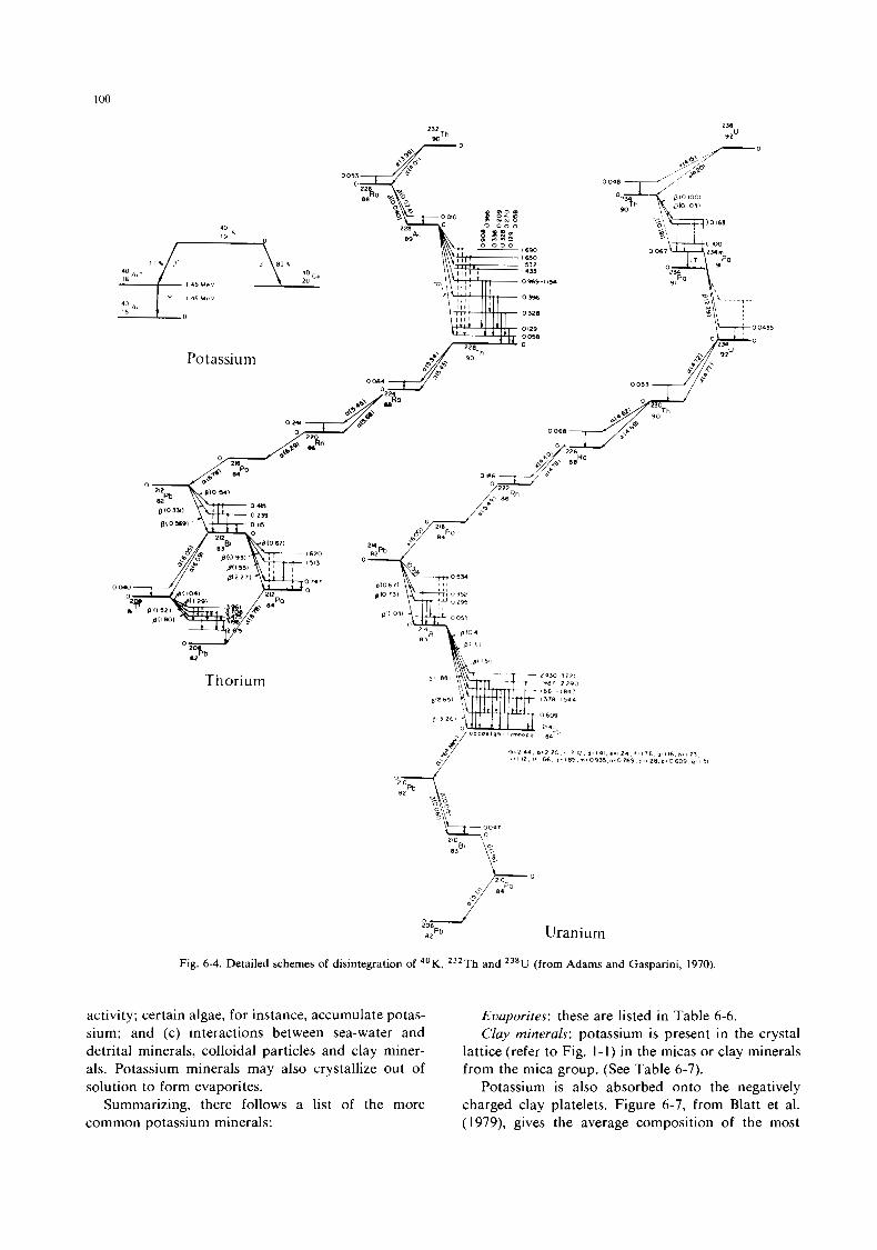
I00
254
92"
19
/
1 46 MeV
Potassium
I 6 9 0 I650 I532 3 433
o 9 6 9 - i i n
0 3%
0 328
0 129
0 o me
0
o& 82
Thorium
"d Pb Uranium 206
82
Fig. 6-4. Detailed schemes of disintegration of 40K, 232Th and 238U (from Adams and Gasparini, 1970).
activity; certain algae, for instance, accumulate potas- sium; and (c) interactions between sea-water and detrital minerals, colloidal particles and clay miner- als. Potassium minerals may also crystallize out of solution to form evaporites.
Summarizing, there follows a list of the more common potassium minerals:
Evaporites: these are listed in Table 6-6. Clay minerals: potassium is present in the crystal
lattice (refer to Fig. 1-1) in the micas or clay minerals from the mica group. (See Table 6-7).
Potassium is also absorbed onto the negatively charged clay platelets. Figure 6-7, from Blatt et al. (1979), gives the average composition of the most
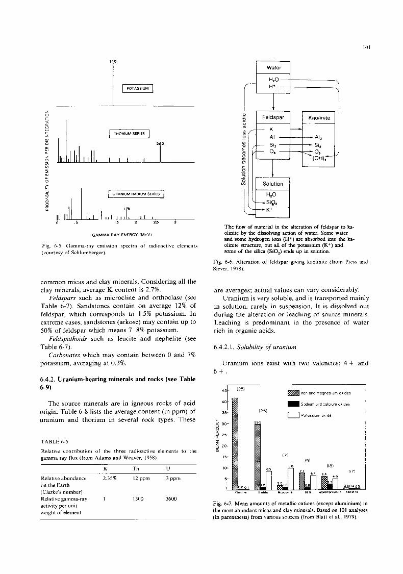
101
I z 0 a U
c s z L" 0
CC w a
z
ul 0 L" 2 Y 0 > L m - 2 0 U n
1, THORIUM SERIES
2.62
dt . 5
I URANIUM-RADIUM SERIES 1
GAMMA RAY ENERGY (MeV1
Fig. 6-5. Gamma-ray emission spectra of radioactive elements (courtesy of Schlumberger).
common micas and clay minerals. Considering all the clay minerals, average K content is 2.7%.
Feldspars such as microcline and orthoclase (see Table 6-7). Sandstones contain on average 12% of feldspar, which corresponds to 1.5% potassium. In extreme cases, sandstones (arkose) may contain up to 50% of feldspar which means 7-8% potassium.
Feldsputhoids such as leucite and nephelite (see Table 6-7).
Carbonates which may contain between 0 and 7% potassium. averaging at 0.3%.
6.4.2. Uranium-bearing minerals and rocks (see Table 6-9)
The source minerals are in igneous rocks of acid origin. Table 6-8 lists the average content (in ppm) of uranium and thorium in several rock types. These
TABLE 6-5
Relative contribution of the three radioactive elements to the gamma ray flux (from Adams and Weaver, 1958)
K Th U
Relative abundance 2.358 12ppm 3 p p m on the Earth (Clarke's number) Relative gamma-ray 1 1300 3600 activity per unit weight of element
Water pi++:
Solution
The flow of material in the alteration of feldspar to ka- olinite by the dissolving action of water. Some water and some hydrogen ions (H+) are absorbed into the ka- olinite structure, but all of the potassium (K+) and some of the silica (SiO,) ends up in solution.
Fig. 6-6. Alteration of feldspar giving kaolinite (from Press and Siever, 1978).
are averages; actual values can vary considerably. Uranium is very soluble, and is transported mainly
in solution, rarely in suspension. It is dissolved out during the alteration or leaching of source minerals. Leaching is predominant in the presence of water rich in organic acids.
6.4.2.1. Solubility of uranium
Uranium ions exist with two valencies: 4 + and 6 + .
Iron and magnesium oxides
Sodium and calcium oxides
0 Potassium oxide
Fig. 6-7. Mean amounts of metallic cations (except aluminium) in the most abundant micas and clay minerals. Based on 101 analyses (in parenthesis) from various sources (from Blatt et al., 1979).
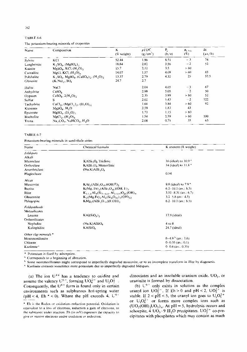
TABLE 6-6
The potassium-bearing minerals of evaporites
Name Composition K p FDC p, ' k ' N I At (%weight) (g/cm') (b/e) (%) (ps/ft)
Sylvitr KCI 52.44 1.86 8.5 I - 3 74 Langbeinite K,SO4. (MgSO4)z 18.84 2.82 3.56 - 2 52 Kainite MgSO4, KCI, (H20)3 15.7 2.12 3.5 > 60 Carnallite MgCL KCI, (H2O), 14.07 1.57 4.09 > 60 83 Polyhalite K2S04, MgSO4, (CasO,),, (H2O)2 13.37 2.79 4.32 25 57.5 Glaseri te (K,Na),. SO4 24.7 2.7
Halite NaCl 2.04 4.65 - 3 67 Anhydrite CaSO, 2.98 5.05 - 2 50 Gypsum CaSO,, 2 ( H 2 0 ) , 2.35 3.99 > 60 52
Tachydrite CaCI,, (MgCI,),, (H20)12 1.66 3.84 > 60 92
Epsomite MgSO4, (H20)7 1.71 1.15 > 60
Sulfur S 2.02 5.43 - 2 122
Kieserite MgSO4, H2O 2.59 1.83 43
Bischofite MgCl,, (H2O), 1.54 2.59 > 60 100 Trona Na,CO,, NaHCO,, H2O 2.08 0.7 1 35 65
TABLE 6-7
Potassium-bearing minerals in sand-shale series
Name Chemical formula K content (% weight)
Feldspurs Alkali Microcline Orthoclase Anorthoclase Plagioclases
Mlcus Muscovite Biotite lllite Glauconite Phlogopite
Felhpathords Metasilicates
Leucite Orthosilicates
Nephelite Kaliophilite
KAISi,O, Triclinic KAlSi,O, Monoclinic (Na.K)AlSi ,O,
KAKSiO, ) 2
(Na. K)A1Si04 KAlSiO,
16 (ideal) to 10.9 * 14 (ideal) to 11.8
0.54
9.8 (ideal) to 7.9 '' 6.2-10.1 (av.: 8.5) 3.51-8.31 (av.: 6.7) 3.2-5.8 (av.: 4.5) 6.2-10.1 (av.: 8.5)
17.9 (ideal)
4 to 8 24.7 (ideal)
Other clay minerals * Montmorilloni te 0-4.9' (av.: 1.6) Chlorite 0-0.35 (av.: 0.1) Kaolinite 0-0.6 (av.: 0.35)
* Potassium is fixed by adsorption. a Corresponds to a beginning of alteration.
Some montmorillonites might correspond to imperfectly degraded muscovite, or to an incomplete transform in illite by diagenesis. Kaolinite contents sometimes more potassium due to imperfectly degraded feldspars.
(a) The ion U4+ has a tendency to oxidize and assume the valency U6+, forming U0:- and U,O:-. Consequently, the U4+ form is found only in certain environments such as sulphurous hot-spring water (pH < 4, Eh * < 0). Where the pH exceeds 4, U4+
dissociates and an insoluble uranium oxide, UO,, or uraninite is formed by dissociation.
(b) U6+ only exists in solution as the complex uranyl ion UO;+. If Eh > 0 and pH < 2, UO;+ is stable. If 2 < pH < 5, the uranyl ion goes to U 2 0 t + or U30i+ or forms more complex ions such as (U0,(OH),U03)n. At pH = 5, hydrolysis occurs and
-
* Eh is the Redox o r oxidation-reduction potential. Oxidation is equivalent t o a loss of electrons. reduction a gain of electrons, to the substance under reaction. Eh (in mV) expresses the capacity to schoepite, u03 ' H2° precipitates. uO;' co-pre-
. .
give or receive electrons under oxidation o r reduction. cipitates with phosphates whch may contain as much
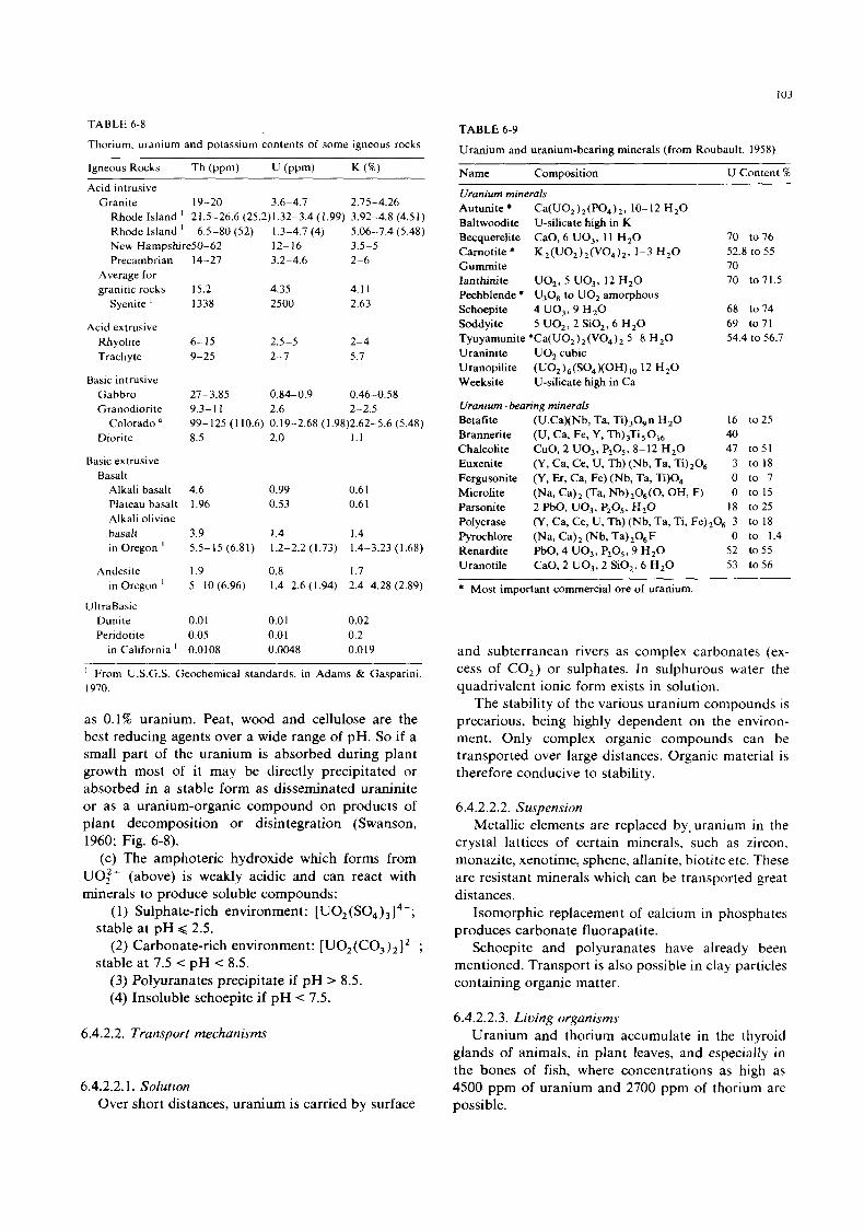
I03
TABLE 6-8
Thorium, uranium and potassium contents of some igneous rocks
Igneous Rocks Th (ppm) U (ppm) K ( W )
Acid intrusive Granite 19-20 3.6-4.7 2.75-4.26
Mode Island ' 21.5-26.6 (25.2)1.32-3.4 (1.99) 3.92-4.8 (4.51) Rhode Island I 6.5-80 (52) 1.3-4.7 (4) 5.06-7.4 (5.48)
Precambrian 14-27 3.2-4.6 2-6 Average for granitic rocks 15.2 4.35 4.11
Syenite ' 1338 2500 2.63
New Hampshire50-62 12-16 3.5-5
Acid extrusive Rhyolite 6- I5 2.5-5 2-4 Trachyte 9-25 2-7 5.7
Basic intrusive Gabbro 27-3.85 0.84-0.9 0.46-0.58 Granodiorite 9.3- 1 I 2.6 2-2.5
Diorite 8.5 2.0 1.1 Colorado a 99-125 ( 1 10.6) 0.19-2.68 (1.9Q2.62-5.6 (5.48)
Basic extrusive Basalt
Alkali basalt 4.6 0.99 0.6 1 Plateau basalt 1.96 0.53 0.61 Alkali olivine basalt 3.9 I .4 I .4 in Oregon ' 5.5-15 (6.81) 1.2-2.2 (1.73) 1.4-3.23 (1.68)
Andesite 1.9 0.8 1.7 in Oregon ' 5- 10 (6.96) 1.4-2.6 (1.94) 2.4-4.28 (2.89)
UltraBasic Dunite 0.01 0.0 1 0.02 Peridotite 0.05 0.01 0.2
in California I 0.0108 0.0048 0.019
I From U.S.G.S. Geochemical standards, in Adams & Gasparini. 1970.
as 0.1% uranium. Peat, wood and cellulose are the best reducing agents over a wide range of pH. So if a small part of the uranium is absorbed during plant growth most of it may be directly precipitated or absorbed in a stable form as disseminated uraninite or as a uranium-organic compound on products of plant decomposition or disintegration (Swanson, 1960; Fig. 6-8).
(c) The amphoteric hydroxide which forms from UOi+ (above) is weakly acidic and can react with minerals to produce soluble compounds:
(1) Sulphate-rich environment: [U0,(S0,),]4-;
(2) Carbonate-rich environment: [UO, (CO,), 1 2-;
(3) Polyuranates precipitate if pH > 8.5. (4) Insoluble schoepite if pH < 7.5.
stable at pH G 2.5.
stable at 7.5 < pH < 8.5.
6.4.2.2. Transport mechanisms
6.4.2.2.1. Solution Over short distances, uranium is carried by surface
TABLE 6-9
Uranium and uranium-bearing minerals (from Roubault. 1958)
Name Composition U Content %
Uranium minerals Autunite Ca(VO,),(PO,),, 10-12 H,O Baltwoodite U-silicate high in K Becquerelite CaO, 6 UO,, 11 H,O 70 to 76 Carnotite * KZ(UO2),(VO4),. 1-3 H,O 52.8 to 55 Gummite 70
70 1071.5 Ianthinite UO,, 5 UO,, 12 H,O Pechblende * U,O, to UO, amorphous
68 to74 Schoepite 4 UO,, 9 H,O Soddyite 5 UO,, 2 SO,, 6 H 2 0 69 to71 Tyuyamunite *Ca(UO,),(VO,), 5-8 H,O 54.4 to 56.7 Uraninite UO, cubic Uranopilite (UO,),(SO,)(OH),, 12 H 2 0 Weeksite U-silicate high in Ca
Uranium -bearing minerals Betafite (U.Ca)(Nb, Ta, Ti)30,n H,O 16 to25
Chalcolite CuO, 2 UO,, P,O,, 8-12 H,O 47 to 51 Euxenite (Y, Ca, Ce, U, Th) (Nb, Ta, Ti),06 3 to 18
Microlite (Na, Ca), (Ta, Nb),O,(O, OH, F) 0 to 15 Parsonite 2 PbO, UO,, P,05, H,O 18 to25 Polycrase to 18
0 to 1.4 Pyrochlore (Na, Ca), (Nb, Ta),06F Renardite PbO, 4 UO,, P,O,, 9 H 2 0 52 to55 Uranotile CaO, 2 UO,, 2 SO,, 6 H,O 53 to56
Brannerite (U, Ca, Fe, Y, Th),TisOl6 40
Fergusonite (Y, Er, Ca, Fe) (Nb, Ta, Ti)O, 0 to 7
(Y, Ca, Ce, U, Th) (Nb, Ta, Ti, Fe) ,06 3
~~~ ~ ~
* Most important commercial ore of uranium.
and subterranean rivers as complex carbonates (ex- cess of CO,) or sulphates. In sulphurous water the quadrivalent ionic form exists in solution.
The stability of the various uranium compounds is precarious, being highly dependent on the environ- ment. Only complex organic compounds can be transported over large distances. Organic material is therefore conducive to stability.
6.4.2.2.2. Suspension Metallic elements are replaced by. uranium in the
crystal lattices of certain minerals, such as zircon. monazite, xenotime, sphene, allanite, biotite etc. These are resistant minerals which can be transported great dis tances.
Isomorphic replacement of calcium in phosphates produces carbonate fluorapatite.
Schoepite and polyuranates have already been mentioned. Transport is also possible in clay particles containing organic matter.
6.4.2.2.3. Living organisms Uranium and thorium accumulate in the thyroid
glands of animals, in plant leaves, and especially in the bones of fish, where concentrations as high as 4500 ppm of uranium and 2700 ppm of thorium are possible.
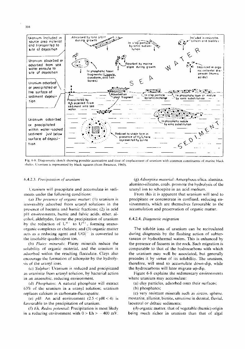
I04
Uroniurn included in soxce ore0 rnateriol cnd t ronspor ted to site ot deposition
Uroniurn absorbed or odsorbed from seo woter enroute to site of deposition
or preci pi toted ot the surfoce of sediment deposi- r
Uroniurn odsorbed
or precipifoted within woter-sooked sediment just below surfoce of deposi- t ion
L A b s o r b e d by mor inr 1 olgor during growlh
1 I n phosphotic foasil ’ f rogmcntr (-0. conodonts,and fish bones1 P
\ i
Stobi l i ied in orgo- nic colloidol d i s - persion (hurnic o c i d r 1
__ ___ ~ ~- ~
~ - _ _ _ -
Fig. 6-8. Diagramatic sketch showing possible association and time of emplacement of uranium with common constituents of marine black shales. Uranium is represented by black squares (from Swanson. 1960).
6.4.2.3. Precipitation of uranium
Uranium will precipitate and accumulate in sedi- ments under the following conditions:
(a ) The presence of organic matter: ( 1 ) uranium is irreversibly adsorbed from uranyl solutions in the presence o f bacteria and humic fractions; (2) in acid pH environments. humic and fulvic acids, ether, al- cohol. aldehydes, favour the precipitation of uranium by the reduction of U h + to U 4 + , forming urano- organic complexes or chelates; and (3) organic matter acts as a reducing agent and UO:+ is converted to the insoluble quadrivalent ion.
(b ) Plutey minerals: Platey minerals reduce the solubility of organic material. and the uranium is adsorbed within the resulting flocculate. Clays also encourage the formation of schoepite by the hydroly- sis of the uranyl ions.
(c) Sulphur: Uranium is reduced and precipitated as uraninite from uranyl solution, by bacterial action in an anaerobic, reducing environment.
(d) Phosphares: A natural phosphate will extract 63% o f the uranium in a uranyl solution; uranium replaces calcium in carbonate-fluorapatite.
(e) p H : An acid environment (2.5 < pH < 4) is favourable to the precipitation of uranium.
( f ) Eh, Redox potential: Precipitation is most likely in a reducing environment with 0 > Eh > -400 mV.
(g) Adsorptive material: Amorphous silica, alumina, alumino-silicates, coals, promote the hydrolysis of the uranyl ion to schoepite in an acid medium.
From this i t is apparent that uranium will tend to precipitate or concentrate in confined, reducing en- vironments, which are themselves favourable to the accumulation and preservation of organic matter.
6.4.2.4. Diagenetic migration
The soluble ions of uranium can be recirculated during diagenesis by the flushing action of subter- ranean or hydrothermal waters. This is enhanced by the presence of fissures in the rock. Such migration is comparable to that of the hydrocarbons with which the uranium may well be associated, but generally precedes it by virtue of its solubility. The uranium, therefore, will tend to accumulate down-dip, while the hydrocarbons will later migrate up-dip.
Figure 6-8 explains the sedimentary environments where uranium may accumulate:
(a) clay particles, adsorbed onto their surfaces; (b) phosphates; (c) very resistant minerals such as zircon, sphene,
monazite, allanite, biotite, xenotime in detrital, fluvial, lacustral or deltaic sediments;
(d) organic matter, that of vegetable (humic) origin being much richer in uranium than that of algal
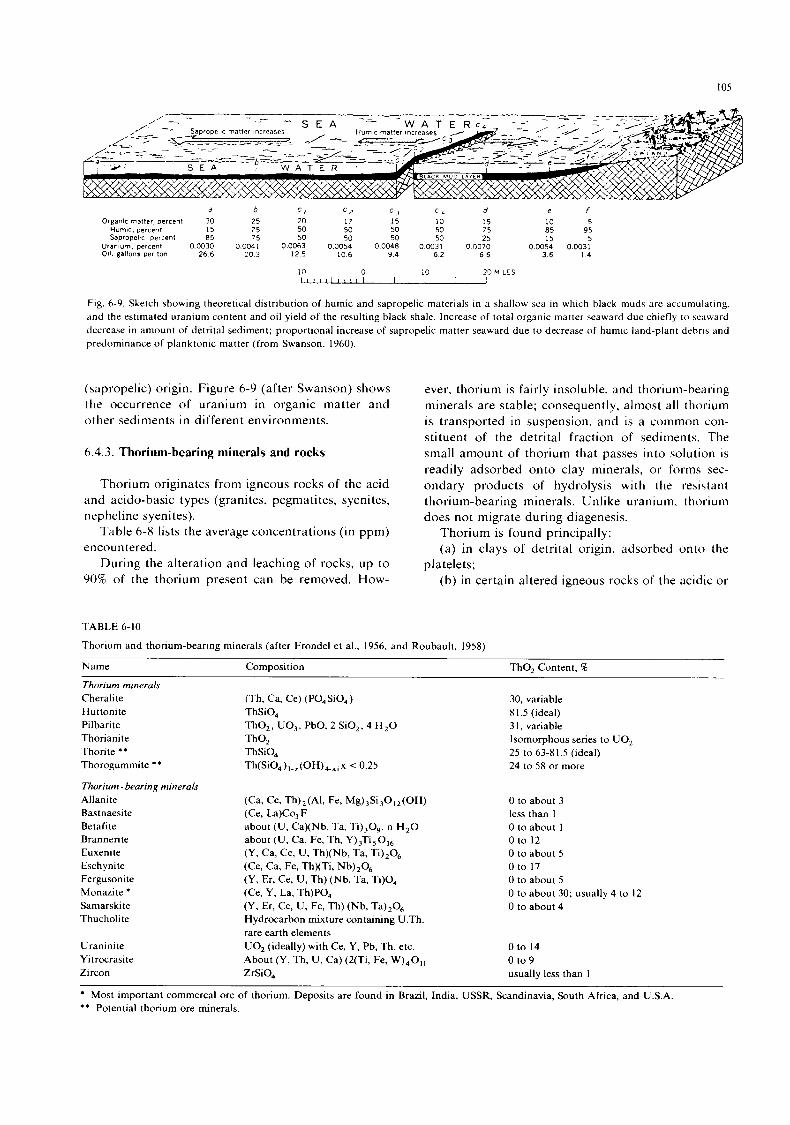
I05
a d e I 6 c / c z c 3 C L
Organic matter, percent 30 25 20 17 15 10 15 10 5 Humic. percent 15 25 50 50 50 50 75 85 95 Sapropeltc. Dercenl 85 75 50 50 50 50 25 15 5
Uranium. percent 0.0030 0.0041 0.0063 0.0054 0.0048 0 0031 0.0370 O.CO54 0.0031 011. gallons per ton 26 6 20 3 12.5 10 6 9 4 6 2 6 6 3.6 1.4
10 0 10 20 MILES I 1 1 1 1 1 1 1 1 1 1 I I I I
Fig. 6-9. Sketch showing theoretical distribution of humic and sapropelic materials in a shallow sea in which black muds are accumulating. and the estimated uranium content and oil yield of the resulting black shale. Increase of total organic matter seaward due chiefly to seaward decrease in amount of detrital sediment; proportional increase of sapropelic matter seaward due to decrease of humic land-plant debris and predominance of planktonic matter (from Swanson, 1960).
(sapropelic) origin. Figure 6-9 (after Swanson) shows the occurrence of uranium in organic matter and other sediments in different environments.
6.4.3. Thorium-bearing minerals and rocks
Thorium originates from igneous rocks of the acid and acido-basic types (granites, pegmatites, syenites, nepheline syenites).
Table 6-8 lists the average concentrations (in ppm) encountered.
During the alteration and leaching of rocks, up to 90% of the thorium present can be removed. How-
ever, thorium is fairly insoluble. and thorium-bearing minerals are stable; consequently, almost all thorium is transported in suspension, and is a common con- stituent of the detrital fraction of sediments. The small amount of thorium that passes into solution is readily adsorbed onto clay minerals, or forms sec- ondary products of hydrolysis with the resistant thorium-bearing minerals. Unlike uranium, thorium does not migrate during diagenesis.
Thorium is found principally: (a) in clays of detrital origin, adsorbed onto the
(b) in certain altered igneous rocks of the acidic or platelets;
TABLE 6-10
Thorium and thorium-bearing minerals (after Frondel et al., 1956. and Roubault, 1958)
Name Composition Tho, Content, %
Thorium minerals Cheralite Huttonite Pilbarite Thorianite Thorite * * Thorogummite **
Thorium - bearing minerals Allanite Bastnaesite Betafite Brannerite Euxenite Eschynite Fergusonite Monazite * Samarski te Thucholite
Uraninite Y i trocrasi te Zircon
(Th, Ca, Ce) (PO,SiO,) ThSiO, Tho, , UO,, PbO, 2 SO,, 4 H,O Tho, ThSiO, Th(SiO,),.,(OH),,,x < 0.25
(Ca, Ce, Th),(Al, Fe, Mg),Si,O,,(OH) (Ce, La)Co,F about (U, Ca)(Nb, Ta, Ti),O,, n H,O about (U, Ca, Fe, Th, Y),Ti,O,, (Y, Ca, Ce, U, Th)(Nb, Ta, Ti),O, (Ce, Ca, Fe, Th)(Ti, Nb),06 (Y, Er, Ce, U, Th) (Nb, Ta, Ti)O, (Ce, Y, La, Th)P04 (Y, Er, Ce, U, Fe, Th) (Nb, Ta),06 Hydrocarbon mixture containing U.Th. rare earth elements UO, (ideally) with Ce, Y, Pb, Th, etc. About (Y. Th, U, Ca) (2(Ti, Fe, W),Oll ZrSiO,
30, variable 8 1.5 (ideal) 3 I , variable Isomorphous series to UO, 25 to 63-81.5 (ideal) 24 to 58 or more
0 to about 3 less than 1 0 to about 1 0 to 12 0 to about 5 0 to 17 0 to about 5 0 to about 30; usually 4 to 12 0 to about 4
0 to 14 0 to 9 usually less than 1
* Most important commercal ore of thorium. Deposits are found in Brazil, India, USSR, Scandinavia, South Africa, and U.S.A * * Potential thorium ore minerals.
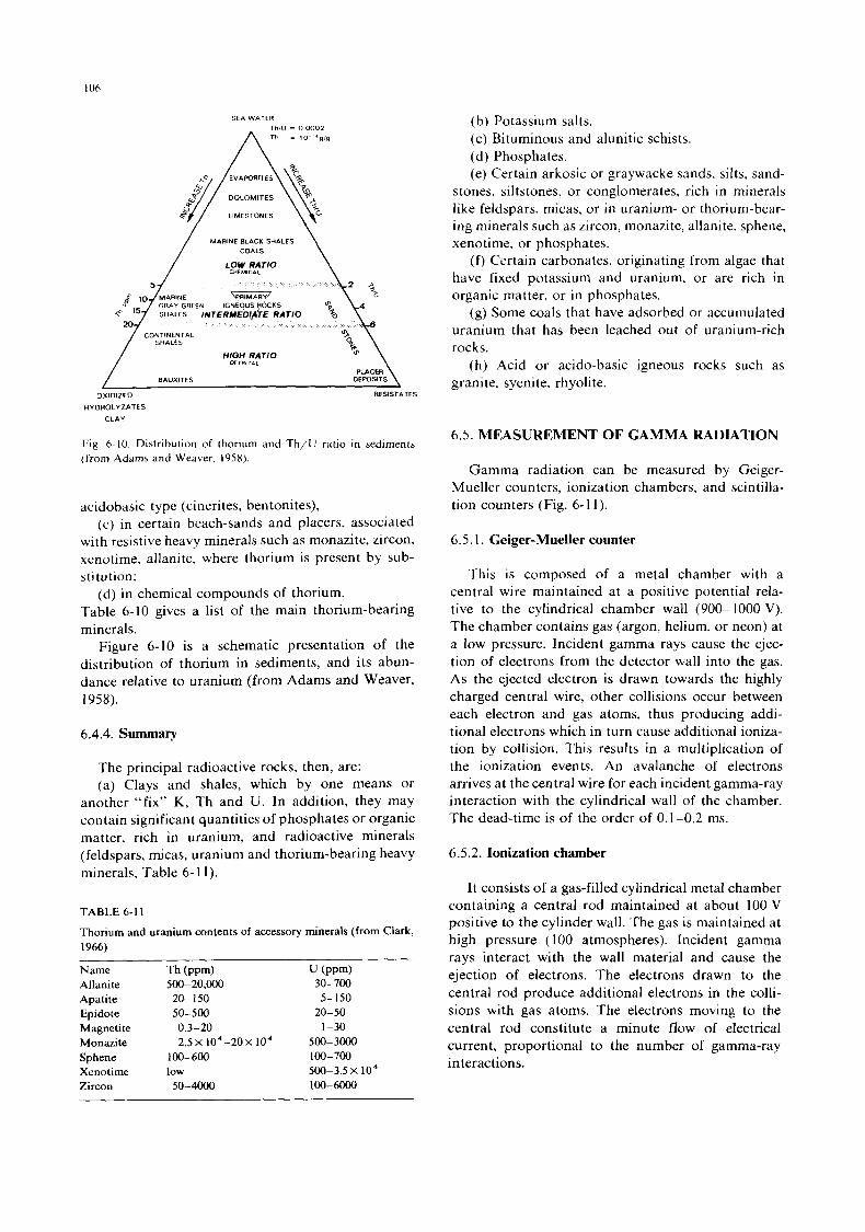
I06
SEA WATER Th/U = 0 0002 A Th = Io-“g/g
LIMESTONES
MARINE BLACK SHALES
CONTINENTAL
HIGH RATIO OCTRITAL
BAUXITES
OXIDIZED RESISTATES
HYDROLYZATES
CLAY
Fig. 6-10. Distribution of thorium and Th/U ratio in sediments ( f rom Adams and Weaver, 1958).
acidobasic type (cinerites, bentonites), (c) in certain beach-sands and placers, associated
with resistive heavy minerals such as monazite, zircon, xenotime, allanite, where thorium is present by sub- sti tution;
Table 6-10 gives a list of the main thorium-bearing minerals.
Figure 6-10 is a schematic presentation of the distribution of thorium in sediments, and its abun- dance relative to uranium (from Adams and Weaver, 1958).
(d) in chemical compounds of thorium.
6.4.4. Summary
The principal radioactive rocks, then, are: (a) Clays and shales, whch by one means or
another “fix” K, Th and U. In addition, they may contain significant quantities of phosphates or organic matter, rich in uranium, and radioactive minerals (feldspars, micas, uranium and thorium-bearing heavy minerals, Table 6-1 1).
TABLE 6-1 1
Thorium and uranium contents of accessory minerals (from Clark, 1966)
Name Th (PPW u (PPW Allanite 500-20,000 30-700 Apatite 20- 150 5-150 Epidote 50-500 20-50 Magnetite 0.3-20 1-30
Sphene 100-600 100-700
Zircon 50-4OOo 100-6000
Monazite 2 . 5 ~ 1o4-2ox 104 500-3000
Xenotime low 500-3.5 x 10⁴
(b) Potassium salts. (c) Bituminous and alunitic schists. (d) Phosphates. (e) Certain arkosic or graywacke sands, silts, sand-
stones, siltstones, or conglomerates, rich in minerals like feldspars, micas, or in uranium- or thorium-bear- ing minerals such as zircon, monazite, allanite, sphene, xenotime, or phosphates.
( f ) Certain carbonates, originating from algae that have fixed potassium and uranium, or are rich in organic matter, or in phosphates.
(g) Some coals that have adsorbed or accumulated uranium that has been leached out of uranium-rich rocks.
(h) Acid or acido-basic igneous rocks such as granite, syenite, rhyolite.
6.5. MEASUREMENT OF GAMMA RADIATION
Gamma radiation can be measured by Geiger- Mueller counters, ionization chambers, and scintilla- tion counters (Fig. 6-1 1).
6.5.1. Geiger-Mueller counter
This is composed of a metal chamber with a central wire maintained at a positive potential rela- tive to the cylindrical chamber wall (900- 1000 V). The chamber contains gas (argon, helium, or neon) at a low pressure. Incident gamma rays cause the ejec- tion of electrons from the detector wall into the gas. As the ejected electron is drawn towards the highly charged central wire, other collisions occur between each electron and gas atoms, thus producing addi- tional electrons which in turn cause additional ioniza- tion by collision. This results in a multiplication of the ionization events. An avalanche of electrons arrives at the central wire for each incident gamma-ray interaction with the cylindrical wall of the chamber. The dead-time is of the order of 0.1-0.2 ms.
6.5.2. Ionization chamber
It consists of a gas-filled cylindrical metal chamber containing a central rod maintained at about 100 V positive to the cylinder wall. The gas is maintained at high pressure (100 atmospheres). Incident gamma rays interact with the wall material and cause the ejection of electrons. The electrons drawn to the central rod produce additional electrons in the colli- sions with gas atoms. The electrons moving to the central rod constitute a minute flow of electrical current, proportional to the number of gamma-ray interactions.
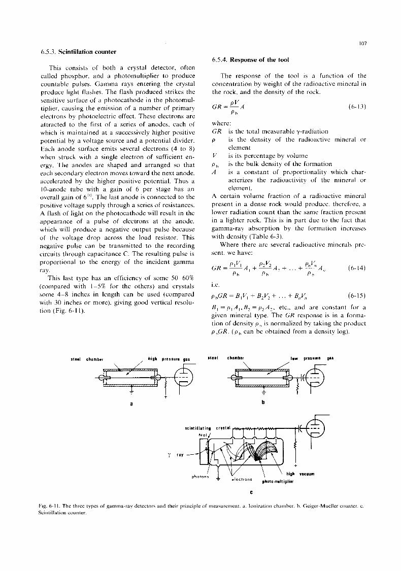
107
6.5.3. Scintillation counter 6.5.4. Response of the tool
This consists of both a crystal detector, often called phosphor, and a photomultiplier to produce countable pulses. Gamma rays entering the crystal produce light flashes. The flash produced strikes the sensitive surface of a photocathode in the photomul- tiplier, causing the emission of a number of primary electrons by photoelectric effect. These electrons are attracted to the first of a series of anodes, each of which is maintained at a successively higher positive potential by a voltage source and a potential divider. Each anode surface emits several electrons (4 to 8) when struck with a single electron of sufficient en- ergy. The anodes are shaped and arranged so that each secondary electron moves toward the next anode, accelerated by the higher positive potential. Thus a 10-anode tube with a gain of 6 per stage has an overall gain of 6"'. The last anode is connected to the positive voltage supply through a series of resistances. A flash of light on the photocathode will result in the appearance of a pulse of electrons at the anode. which will produce a negative output pulse because of the voltage drop across the load resistor. This negative pulse can be transmitted to the recording circuits through capacitance C. The resulting pulse is proportional to the energy of the incident gamma ray.
This last type has an efficiency of some 50-60% (compared with 1-5% for the others) and crystals some 4-8 inches in length can be used (compared with 30 inches or more), giving good vertical resolu- tion (Fig. 6-1 1).
The response of the tool is a function of the concentration by weight of the radioactive mineral in the rock, and the density of the rock.
PV GR=-A Ph
(6-13)
where: GR is the total measurable y-radiation p is the density of the radioactive mineral o r
element V is its percentage by volume ph is the bulk density of the formation A is a constant of proportionality which char-
acterizes the radioactivity o f the mineral o r element.
A certain volume fraction of a radioactive mineral present in a dense rock would produce, therefore, a lower radiation count than the same fraction present in a lighter rock. This is in part due to the fact that gamma-ray absorption by the formation increases with density (Table 6-3).
Where there are several radioactive minerals pre- sent, we have:
1.e.
phGR = B,V, + B2V2 + ... + B,,I.;, (6-15)
B , =p,A, ,B ,=p,A, , etc., and are constant for a given mineral type. The GR response is in a forma- tion of density ph is normalized by taking the product p,,GR. (ph can be obtained from a density log).
steel chamber IOW pressure gas steel chamber
a +
ll
scintil lating crystal
'I ray
\ \ high vacuum
photo multiplier photon! 1 - e l e c t r o n s
C
Fig. 6-1 I . The three types of gamma-ray detectors and their principle of measurement. a. Ionization chamber. h. Geiger-Mueller counter. c. Scintillation counter.
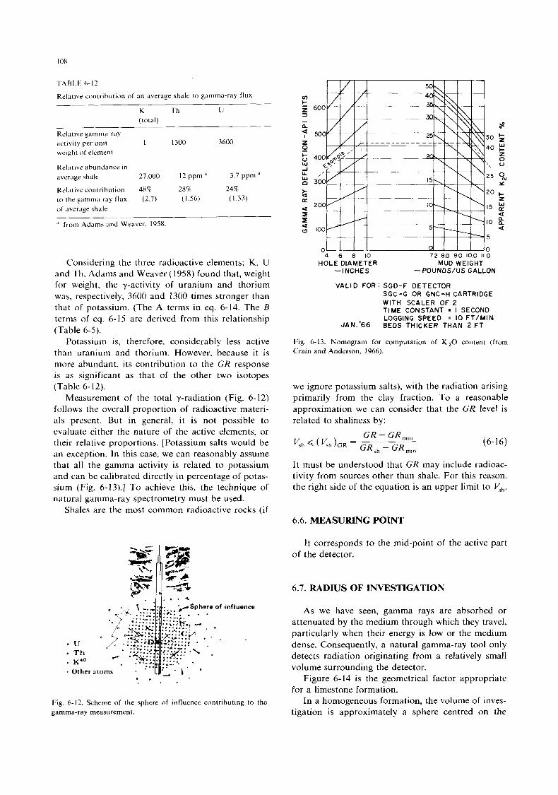
TABLE 6-12
Relative contrihution o f an average shale to gamma-ray flux
K Th U (total)
Relative gamma-ray ;ictivity per unit 1 1300 3600 weight of element
Kelatlve abundance in average shale 27.000 12 ppm 3.7 ppm *
Relative contrihution 48% 28% 24% to the gamma ray flux (2.7) (1.56) ( 1.33) of average shale
I' from Adams and Weaver. 1958.
Considering the three radioactive elements; K, U and Th, Adams and Weaver (1958) found that, weight for weight, the y-activity of uranium and thorium was, respectively, 3600 and 1300 times stronger than that of potassium. (The A terms in eq. 6-14. The B terms of eq. 6-15 are derived from this relationship (Table 6-5).
Potassium is, therefore, considerably less active than uranium and thorium. However, because it is more abundant, its contribution to the GR response is as significant as that of the other two isotopes (Table 6-12).
Measurement of the total y-radiation (Fig. 6-12) follows the overall proportion of radioactive materi- als present. But in general, i t is not possible to evaluate either the nature of the active elements, or their relative proportions. [Potassium salts would be an exception. In this case, we can reasonably assume that all the gamma activity is related to potassium and can be calibrated directly in percentage of potas- sium (Fig. 6-13).] To achieve this, the technique of natural gamma-ray spectrometry must be used.
Shales are the most common radioactive rocks ( i f
. .
Fig. 6-12. Scheme of the sphere of influence contributing to the gamma-ray measurement
4 6 8 1 0 HOLE DIAMETER
72 80 90 100 I 1 0 MUD WEIGHT
--INCHES -POUNDS/US GALLON
VAL1 D FOR : SGD-F DETECTOR SGC-G OR GNC-H CARTRIDGE WITH SCALER OF 2 TIME CONSTANT = I SECOND LOGGING SPEED = 10 FT/MIN
JAN.'66 BEDS THICKER THAN 2 F T
Fig. 6-13. Nomogram for computation of K,O content (from Crain and Anderson, 1966).
we ignore potassium salts), with the radiation arising primarily from the clay fraction. To a reasonable approximation we can consider that the GR level is related to shaliness by:
GR - GR,,,
G R , h - GR, in K h ( K h ) , , = (6-16)
It must be understood that GR may include radioac- tivity from sources other than shale. For this reason, the right side of the equation is an upper limit to yh.
6.6. MEASURING POINT
It corresponds to the mid-point of the active part of the detector.
6.7. RADIUS OF INVESTIGATION
As we have seen, gamma rays are absorbed or attenuated by the medium through which they travel, particularly when their energy is low or the medium dense. Consequently, a natural gamma-ray tool only detects radiation originating from a relatively small volume surrounding the detector.
Figure 6-14 is the geometrical factor appropriate for a limestone formation.
In a homogeneous formation, the volume of inves- tigation is approximately a sphere centred on the
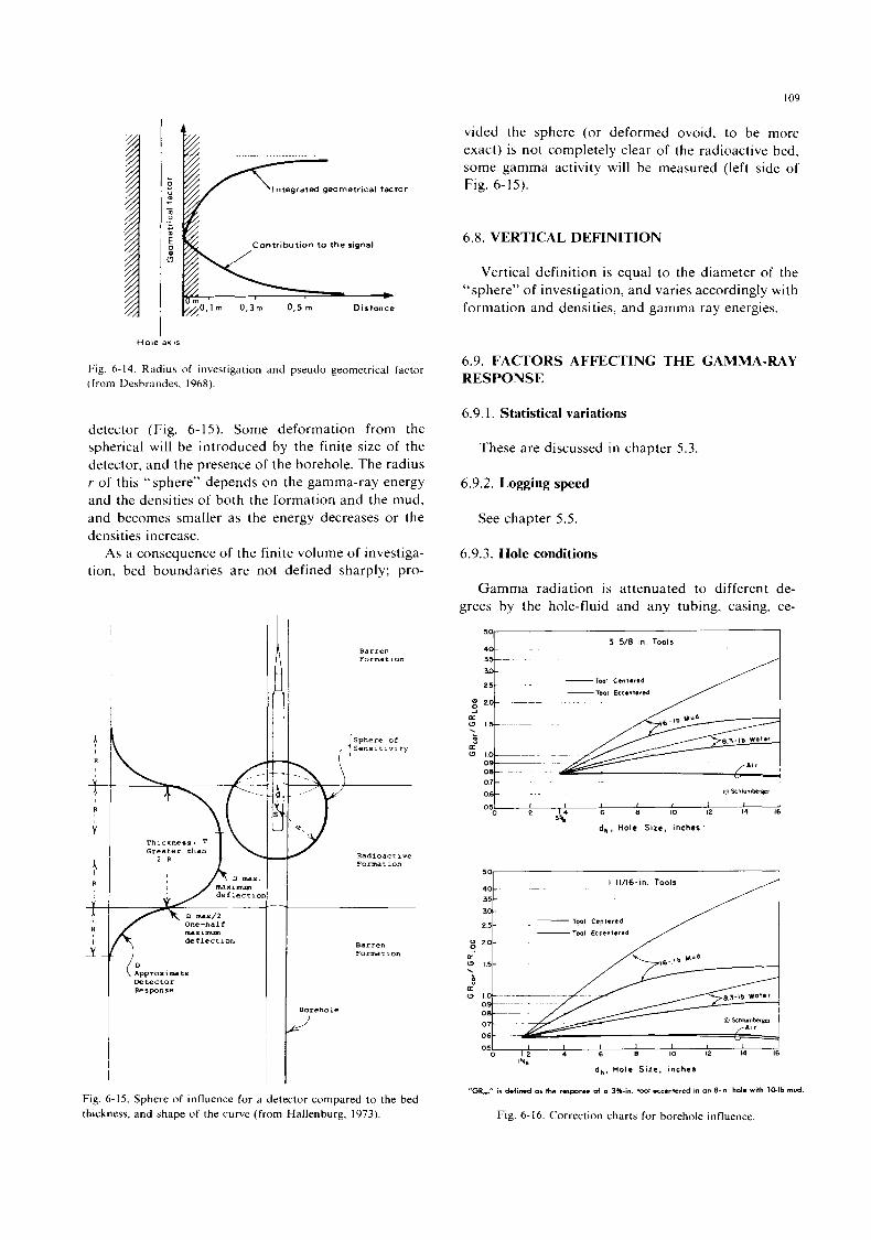
I09
.. ... . ... ~ .............. ~.~~~~~~
I n t e g r a t d geometrical factor
Contr ibut ion t o the signal
Distance
I Hole axis
Fig. 6-14. Radius of investigation and pseudo geometrical factor (from Desbrandes. 1968).
detector (Fig. 6- 15). Some deformation from the spherical will be introduced by the finite size of the detector. and the presence of the borehole. The radius r of this “sphere” depends on the gamma-ray energy and the densities of both the formation and the mud, and becomes smaller as the energy decreases or the densities increase.
As a consequence of the finite volume of investiga- tion, bed boundaries are not defined sharply; pro-
d R
Response
Formation
Barren Formation
Borehole
LJ
Fig. 6-15. Sphere o f influence for a detector compared to the bed thickness, and shape of the curve (from Hallenburg, 1973).
vided the sphere (or deformed ovoid, to be more exact) is not completely clear of the radioactive bed, some gamma activity will be measured (left side of Fig. 6-15).
6.8. VERTICAL DEFINITION
Vertical definition is equal to the diameter of the “sphere” of investigation, and varies accordingly with formation and densities, and gamma ray energies.
6.9. FACTORS AFFECTING THE GAMMA-RAY RESPONSE
6.9. I . Statistical variations
These are discussed in chapter 5.3.
6.9.2. Logging speed
See chapter 5.5.
6.9.3. Hole conditions
Gamma radiation is attenuated to different de- grees by the hole-fluid and any tubing. casing. ce-
3 5/8 in Tools
Tool Cen1.r.d
-Tool Eccen1.r.d
07
06
05 2 $4 6 8 10 12 14 16
0 Schl“rnbe.ne,
I I I I I I
d,. Hole Size . inches
I l l / l6-1n Tools
Tool C a n l o e d
Tool Eccentercd
I I I I I I I 4 6 8 10 12 14 16 0 I 2
“%6
051
d,,, H o l e Size, inches
“GL,’’ is defined as the r e s ~ n s e of D 3%n. t-I ecccntcred in an 8-in. hole with 104b mud.
Fig. 6-16. Correction charts for borehole influence
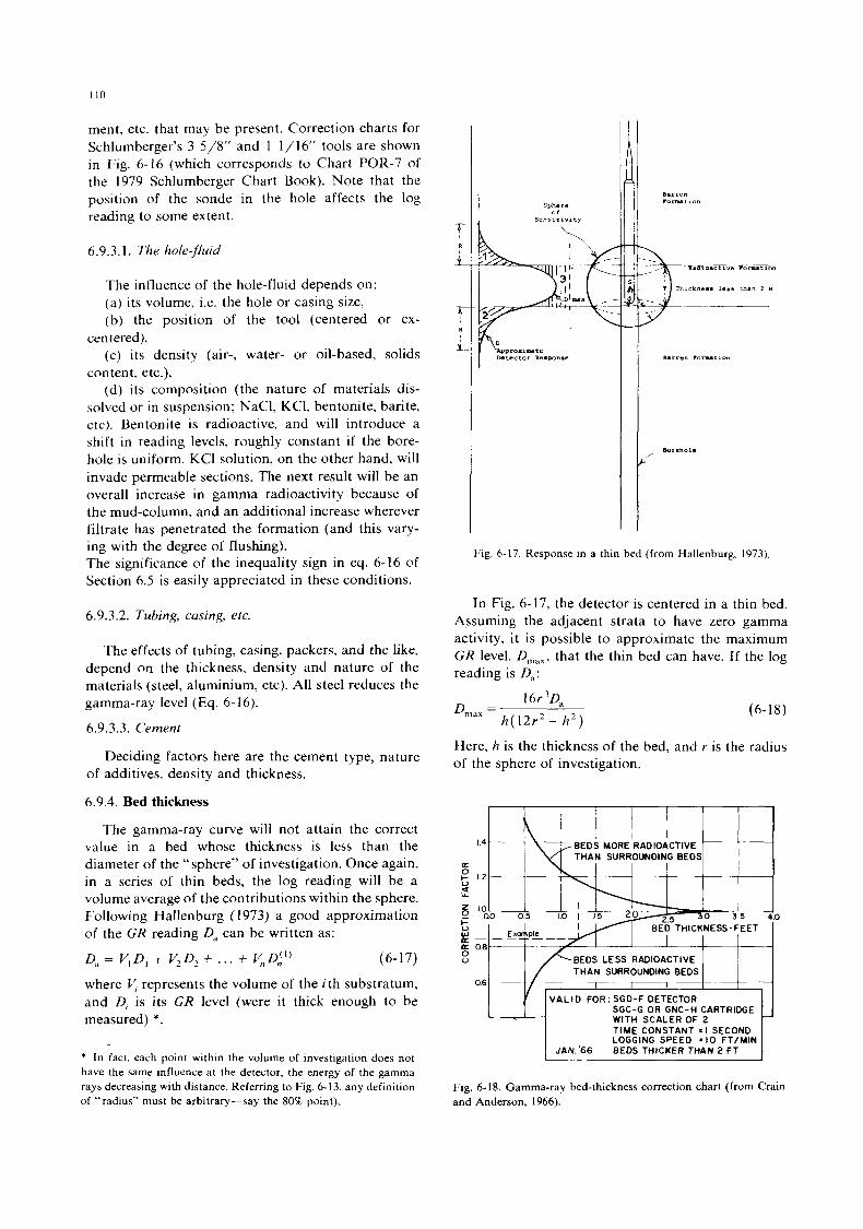
110
ment, etc. that may be present. Correction charts for Schlumberger's 3 5/8" and 1 1/16" tools are shown in Fig. 6-16 (which corresponds to Chart POR-7 of the 1979 Schlumberger Chart Book). Note that the position of the sonde in the hole affects the log reading to some extent.
6.9.3.1. The hole-fluid
The influence of the hole-fluid depends on: (a) its volume, i.e. the hole or casing size, (b) the position of the tool (centered or ex-
centered), (c) its density (air-, water- or oil-based, solids
content, etc.), (d) its composition (the nature of materials dis-
solved or in suspension; NaC1, KCl, bentonite, barite, etc). Bentonite is radioactive, and will introduce a shift in reading levels, roughly constant if the bore- hole is uniform. KCl solution, on the other hand, will invade permeable sections. The next result will be an overall increase in gamma radioactivity because of the mud-column, and an additional increase wherever filtrate has penetrated the formation (and t h s vary- ing with the degree of flushing). The significance of the inequality sign in eq. 6-16 of Section 6.5 is easily appreciated in these conditions.
6.9.3.2. Tubing, casing, etc.
The effects of tubing, casing, packers, and the like, depend on the thickness, density and nature of the materials (steel, aluminium, etc). All steel reduces the gamma-ray level (Eq. 6- 16).
6.9.3.3. Cement
Deciding factors here are the cement type, nature of additives, density and thickness.
6.9.4. Bed thickness
The gamma-ray curve will not attain the correct value in a bed whose thickness is less than the diameter of the "sphere" of investigation. Once again, in a series of thin beds, the log reading will be a volume average of the contributions within the sphere. Following Hallenburg (1973) a good approximation of the GR reading D, can be written as:
Da = V , D , -t &Dz + ... f V,Dd" (6-17)
where V , represents the volume of the i th substratum, and 0, is its GR level (were i t thick enough to be measured) *.
~~
* In fact. each point within the volume of investigation does not have the same influence at the detector, the energy of the gamma rays decreasing with distance. Referring to Fig. 6-13, any definition o f "radius" must be arbitrary-say the 80% point).
7-
i R
T
i R
Borehole /
'ig. 6-17. Response in a thin bed (from Hallenburg. 1973)
In Fig. 6-17, the detector is centered in a thin bed. Assuming the adjacent strata to have zero gamma activity, i t is possible to approximate the maximum GR level, D,,,, that the thin bed can have. If the log reading is 0,:
(6-18)
Here, h is the thickness of the bed, and r is the radius of the sphere of investigation.
BEDS MORE RADIOACTIVE
LL
u
BEDS LESS RADIOACTIVE THAN SURROUNDING BEDS
VALID FOR: SGD-F DETECTOR SGC-G OR GNC-H CARTRIDGE WITH SCALER OF 2 TIME CONSTANT =I SECOND LOGGING SPEED =I0 FT/MIN BEDS THICKER THAN 2 F T JAN.'66
Fig. 6-18. Gamma-ray bed-thickness correction chart (from Crain and Anderson, 1966).
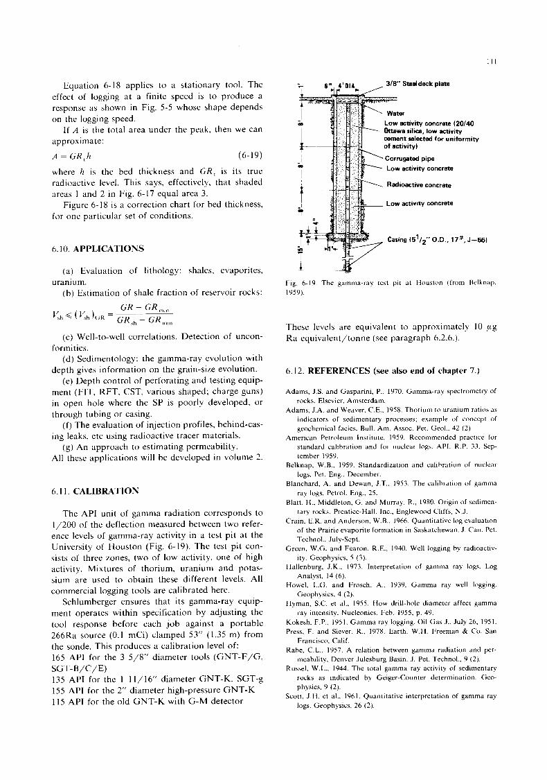
Equation 6-18 applies to a stationary tool. The effect of logging at a finite speed is to produce a response as shown in Fig. 5-5 whose shape depends on the logging speed.
I f A is the total area under the peak, then we can approximate: A = G R , h (6-19)
where h is the bed thickness and G R , is its true radioactive level. This says, effectively, that shaded areas 1 and 2 in Fig. 6-17 equal area 3.
Figure 6- 18 is a correction chart for bed thickness, for one particular set of conditions.
6.10. APPLICATIONS
(a) Evaluation of lithology: shales, evaporites,
(b) Estimation of shale fraction of reservoir rocks: uranium.
(c) Well-to-well correlations. Detection of uncon- formi ties.
(d) Sedimentology: the gamma-ray evolution with depth gives information on the grain-size evolution.
(e) Depth control of perforating and testing equip- ment (FIT, RFT, CST, various shaped; charge guns) in open hole where the SP is poorly developed, or through tubing or casing.
(f) The evaluation of injection profiles, behind-cas- ing leaks, etc using radioactive tracer materials.
(8) An approach to estimating permeability. All these applications will be developed in volume 2.
6.1 1. CALIBRATION
The API unit of gamma radiation corresponds to 1/200 of the deflection measured between two refer- ence levels of gamma-ray activity in a test pit at the University of Houston (Fig. 6-19). The test pit con- sists of three zones, two of low activity, one of high activity. Mixtures of thorium, uranium and potas- sium are used to obtain these different levels. All commercial logging tools are calibrated here.
Schlumberger ensures that its gamma-ray equip- ment operates within specification by adjusting the tool response before each job against a portable 266Ra source (0.1 mCi) clamped 53“ (1.35 m) from the sonde. This produces a calibration level of: 165 API for the 3 5/8” diameter tools (GNT-F/G,
135 API for the 1 11/16” diameter GNT-K, SGT-g 155 API for the 2” diameter high-pressure GNT-K 115 API for the old GNT-K with G-M detector
SGT-B/C/E)
% 6 ’ i ? ’ D l A = , 318’ Steeldeck plate
i
I I / r
Fig. 6-19. The gamma-ray test pit at Houston (from Belknap. 1959).
These levels are equivalent to approximately 10 pg Ra equivalent/tonne (see paragraph 6.2.6.).
6.12. REFERENCES (see also end of chapter 7.)
Adams, J.S. and Gasparini, P., 1970. Gamma-ray spectrometry of rocks. Elsevier, Amsterdam.
Adams, J.A. and Weaver, C.E., 1958. Thorium t o uranium ratios as indicators of sedimentary processes; example of concept of geochemical facies. Bull. Am. Assoc. Pet. Geol.. 42 (2).
American Petroleum Institute, 1959. Recommended practice for standard calibration and for nuclear logs. API. R.P. 33. Sep- tember 1959.
Belknap. W.B., 1959. Standardization and calibration of nuclear logs. Pet. Eng., December.
Blanchard, A. and Dewan, J.T.. 1953. The calibration of gamma ray logs. Petrol. Eng., 25.
Blatt. H., Middleton, G. and Murray, R., 1980. Origin of sedimen- tary rocks. Prentice-Hall, Inc.. Englewood Cliffs, N.J.
Crain. E.R. and Anderson. W.B., 1966. Quantitative log evaluation of the Prairie evaporite formation in Saskatchewan. J. Can. Pet. Technol., July-Sept.
Green, W.G. and Fearon. R.E., 1940. Well logging by radioactiv- ity. Geophysics, 5 (3).
Hallenburg, J.K., 1973. Interpretation of gamma ray logs. Log Analyst, 14 (6).
Howel, L.G. and Frosch. A,, 1939. Gamma ray well logging. Geophysics, 4 (2).
Hyman, S.C. et al.. 1955. How drill-hole diameter affect gamma ray intensity. Nucleonics. Feb. 1955, p. 49.
Kokesh, F.P.. 1951. Gamma ray logging. Oil Gas J.. July 26. 1951. Press, F. and Siever, R., 1978. Earth. W.H. Freeman & Co. San
Francisco. Calif. Rabe, C.L.. 1957. A relation between gamma radiation and per-
meability. Denver Julesburg Basin. J. Pet. Technol.. 9 (2). Russel, W.L., 1944. The total gamma ray activity of sedimentary
rocks as indicated by Geiger-Counter determination. Geo- physics, 9 (2).
Scott, J.H. et al., 1961. Quantitative interpretation of gamma ray logs. Geophysics, 26 (2).

I12
Swanson, V.E.. 1960. Oil yield and uranium content of black
Tittman. J.. 1956. Radiation logging: physical principles. In: Univ.
Tixier, M.P. and Alger. R.P., 1967. Log evaluation of non metallic
shales. U.S. Geol. Surv.. Prof. Pap., 356-A.
Kansas Petroleum Eng. Conf.. April 2 and 3, 1956.
mineral deposits. SPWLA. 8th Annu. Symp. Trans., paper R.
Toelke, L.W., 1952. Scintillometer used in radiation logging. World
Westby, G.H. and Scherbatskay, S.A.. 1940. Well logging by Oil. 135 (3).
radioactivity. Oil Gas. J.. 38 (41).
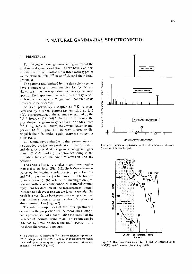
113
7. NATURAL GAMMA-RAY SPECTROMETRY
7.1. PRINCIPLES
For the conventional gamma-ray log we record the total natural gamma radiation. As we have seen, this radiation is in fact emitted from three main types of source elements: 40K, 232Th or 23xU, (and their decay products).
The gamma rays emitted by the three decay series have a number of discrete energies. In Fig. 7-1 are shown the three corresponding gamma-ray emission spectra. Each spectrum characterizes a decay series, each series has a spectral “signature” that enables its presence to be discerned.
As seen previously (Chapter 6) 40K is char- acterized by a single gamma-ray emission at 1.46 MeV. corresponding to the gamma ray emitted by the 40Ar* isotope (Fig. 6-4) *. In the 232Th series, the most distinctive gamma-ray peak is at 2.62 MeV from *“‘Tl, Fig. 6-5), but there are several lower energy peaks. The 2‘4Bi peak at 1.76 MeV is used to dis- tinguish the 238U series; again, there are numerous other peaks.
But gamma rays emitted with discrete energies can be degraded by: (a) pair production in the formation and detector crystal, i f the gamma energy is higher than 1.02 MeV; and (b) Compton scattering in the formation between the point of emission and the detector.
The observed spectrum takes a continuous rather than a discrete form (Fig. 7-2). Such degradation is worsened by logging conditions (compare Fig. 7-2 and 7-1). I t is due to: (a) limitation of detector size (poor efficiency); (b) volume of investigation (im- portant. with large contribution of scattered gamma rays); and (c) duration of the measurement (limited in order to achieve a reasonable logging speed). The result is a very large background in the spectrum, so that its fine structure, given by about 50 peaks, is almost entirely lost (Fig. 7-2).
The relative amplitudes of the three spectra will depend on the proportions of the radioactive compo- nents present, so that a quantitative evaluation of the presence of thorium, uranium and potassium can be obtained by breaking down the total spectrum into the three characteristic spectra.
1.46
(1
z 0 - L
Y 0 >
URANIUM-RADIUM SERIES
a
.5 1.6 2 25 3
G A M M A RAY ENERGY (MeV)
Fig. 7-1. Gamma-ray emission spectra of radioactive elements (courtesy of Schlumberger).
* 1 1 percent of the decays of 40K involve electron capture and 40Ar* is the product. The 40Ar* is, however, in an unstable excited state, and upon returning to its ground-state, emits the gamma photon at 1.46 MeV (Fig. 6-4).
ENERGV OF GAMMA RAVS ( M i V l
Fig. 7-2. Real Spectrograms of K, Th and U obtained from NaI(T1) crystal detector (from Doig, 1968).
This analysis will only be valid if we can assume that the spectra of the three radioactive series always have the same energy distribution. As thorium and uranium series are normally in a state of secular equilibrium, each series has the characteristic spec- trum observed on Fig. 7-1 with the different elements occurring in fairly well-defined proportions.
To obtain a quantitative evaluation of thorium. uranium and potassium from an analysis of the total energy distribution, i t is helpful to divide the spec- t rum into two regions:
( 1 ) The high-energy region, with three main peaks: Thallium ’“‘Tl at 2.62 MeV (from the 232Th family) Bismuth ‘I4Bi at 1.76 MeV (from the ’”U family) Potassium 40K at 1.46 MeV
(2) The low-energy region, covering the energy range of the gamma rays resulting from Compton scattering in the formation, plus lower-energy emis- sions from the thorium and uranium series.
7.2. TOOL DESCRIPTION
The Dresser Atlas Spectralog” tool measures the counting rates in a number of “windows”, each of which spans a certain energy band. As can be seen from Fig. 7-3 the high-energy region is divided into three windows (W 3, W 4 and W 5), centered on the three characteristic high-energy peaks. Thus, broadly speaking, we can see that these three windows will have responses corresponding to the amounts of thorium, uranium and potassium respectively. There will be a certain amount of correlation (for example, i t is clear that window 3 will respond not only to the presence of potassium, but also to some extent to the presence of uranium and thorium). However, with three windows i t is possible to compute the exact solution:
232Th = m,,W3 + m14W4 + m,5W5 (7-1)
7.3. DETECTOR
The detector consists of a sodium iodide crystal doped with thallium-referred to as NaI (TI). It is optically coupled to a photo-multiplier (Fig. 7- lo), and an amplifier and a multi-channel analyser com-
ENERGY OF G A M M A RAY (MeV)
Fig. 7-3. Window repartition in the Dresser Atlas’ Spectralog.
’” u = rn 2 3 ~ 3 + m 2 4 ~ 4 + rn 2 s ~ 5
40K = m,,W, + m3,W4 + m,,W,
(7-2)
(7-3)
where m,, is the current element of the so-called measurement matrix.
The Schlumberger Natural Gamma ray Spectrom- etry tool (NGS *) uses five windows (Fig. 7-4), mak- ing fuller use of the information in the spectrum so as to reduce the statistical uncertainty on the analysis of Th, U and K. Indeed the high-energy region repre- sents only ten percent of the spectrum in terms of counting rates. As a result, the above computations are subject to a very substantial statistical error.
Much-improved results can be obtained if we take into consideration the remaining (low-energy) portion of the detectable spectrum. Ths region contains meaningful information that is pertinent to the spec- trometry measurement.
Figure 7-5, from Marett et al. (1976), compares the result of a three-window analysis with one incorpo- rating low-energy information. The reduction in sta- tistics is clearly seen in the second case: the standard deviation of the statistical noise for Th, U and K is reduced substantially (Fig. 7-6).
To illustrate the importance of the low-energy windows an artifical log was created. By adding statistical variations to a theoretical model (Fig. 7-7), whch assumes a succession of levels with different thorium, uranium and potassium content, artificial window count-rates were created (Fig. 7-8). As we observe, small peaks on thorium, uranium or potas- sium are only clearly seen on the low-energy windows. On the high-energy windows, these peaks are difficult to separate from the statistical noise. To define the sensitivity of the tool another artificial log was created (Fig. 7-9) in which a sequence of thorium, uranium and potassium peaks was created. Even if the spec- trum is degraded by Compton scattering it appears that the low-energy windows are the most sensitive: compared to a constant background, peaks of 1 ppm uranium, 2 ppm thorium and 0.3% potassium are detected only on the two first low-energy windows and do not appear on the three high-energy windows where they are masked by statistics.
* Trade Mark of Schlumberger. Although the NGS spectrum is degraded, mainly by Compton scattering, i t can be retrieved by statistical analysis.
PROBABILITY OF EMISSION PER OESINTEGRATION
3 - b
0 5
0 2 - a n
2
I-
Y 0
U
z U I- m
I- 2
Yt ’ -
I (T:+U+K)
I
0 1 2 - Energy I M ~ V I
I Schlumbergsr Wndovs wz I w3 I w4 I W5
HIGH ENERGY “ W l i
LOW ENERGY HIGH COUNT RATE LOW COUNT RATE
Y I
Fig. 7-4. Potassium, Thorium and Uranium response curve (NaI crystal detector) (from Serra et al., 19x0).
T h F
I I I
WHITOUT CONTRIBUTON ” FROM LOW ENERGY WINDOWS
I - k
WITH CONTRl0UTlON FROM LOW ENIRGV WINDOWS
I I I
I -m Flg. 7-5. Gamma-ray spectrometry with and without low-energy windows (from Marett et al.. 1976).
T I M E C O N S T A N T 8 LOGGING S P E E D = 900 F T / H R
4 S E C
Th3
0 Th5 SUBSCRIPTS 3, 5 - NUMBER OF
WINOOWS
- FILTERING
0 u5
O K F , - 0 4 8 12
A V E R A G E M E A S U R E M E N T V A L U E
Fig. 7-6. NGS statistical error (from Serra et al., 1980).
plete the measuring circuitry. Unlike previous gamma-ray tools, which only counted pulses, the energy determination of the gamma rays entering the crystal is of the utmost importance.
Figure 7-11 shows how the proportionality be- tween the energy E of the gamma ray entering the crystal and the output voltage Vat the preamplifier is achieved (see figure caption).
The pulse amplitude V is analyzed by a set of comparators each of which has a fixed reference voltage. The window count rates obtained by these comparators are stored in a buffer and sent to the surface through the telemetry. The purpose of the feedback loop, shown on the downhole block dia- gram of Fig. 7-10, is to stabilize the gamma spectrum in energy. It uses a reference gamma-ray source and can be considered as a continuous energy calibration of the tool. Since the behaviour of the detector versus temperature is unpredictable, this stabilization is es- sential.
At the surface, the transmitted information is de- coded and made available for further digital processing in the CSU mode. For optical display the data are depth-averaged. In this averaging technique the data sampled at one depth are averaged with data sampled just before (past) and just after (future), before being recorded on film. This gives a symmetric curve in time with no lag related to logging speed. A further reduction in the statistical noise is achieved using the filtering technique described later. The standard gamma ray, GR, along with the filtered Th, U, K and “ uranium-free’’ gamma-ray measurement, CGR, are available for playback at the well-site with the CSU system.
1 I6
0 Th 80 ’ 30
0 fppm’ K 10
(PPml ” 0
1%)
9700
9800
Fig. 7-7. Main log. Model.
A time-constant of 4 seconds was used for logging the NGS-tool at 900 ft/hr with panel. A time-con- stant of 6 seconds and a recording speed of 600 ft/hr are required for the Spectralog. With the CSU sys- tem, the measurement time is fixed and samples are taken every six inches of tool travel. The sampling time chosen is sufficient to maintain the standard deviation at less than 2.5%, when the standard log- ging speed is used (900 ft/hr).
r
0 wi 400 0 W2 400
0 w3 400
7
9700
I
Fig. 7-8. Main log. Window counts (in cps).
7.4. CALIBRATION
For Schlumberger’s tools, the base of the master calibration is a special test pit (TUK pit) which has been built in Clamart (Fig. 7-12).
The basic structure of this pit consists of four zones. Each of the top three zones contains the three radioactive elements, thorium, uranium and potas- sium, with the greatest possible contrast between the zones.
a
117
b I
9700
9800
i- I
Fig. 7-9. a. Model for testing the sensitivity. Th. U. K computation using a Kalrnan filter. b. Model for testing the sensitivity. Windoh counts ( in cps).
A fourth zone, at the bottom of the pit, enables the descent of long tools and the evaluation of the radio- active contribution of the concrete that is the main component of the lower zone. The size of the pit was dictated by the most powerful radiation emitted by the components, i.e. the 2.62 MeV gamma ray of the thorium series.
The NGS calibration involves the measuring of the counting rates in the five windows when the tool is placed in the centre of the three zones.
The counting rate in window i when the tool is placed in zonej is called y,. There are 15 y , values.
These values are related to the Th,, U,, K , contents by the linear relations:
W;,=A,Th,+ B,U, + C,K, (7-4)
where Th,, U,, K, are known and I+(, measured.
resolving the 3 equations system: The 15 coefficients A , , B , , C, are computed by
W;, =A,Th, + B,U, + C,K,
W;* = A,Th, + B,U, + C , K 2
W;, = A,Th, + B,U, + C,K,
(zone 1 )
(zone 2)
(zone 3)
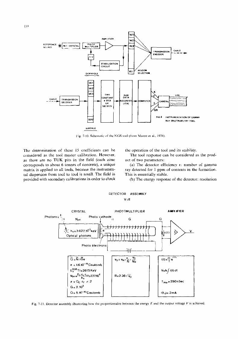
REFERENCE SOURCE
L AMPI, I F I E R
TRANSMISSION ENCODER
SELECT- W W N H O L E
SURFACE
CABLE -----)
I I I I
4 SECS ECORDER OR
im SECS
LOG
4 SECS ECORDER
:ONSTANT
im SECS
FIG.6 INSTRUMENTATION OF GAMMA
RAY SPECTROMETRY TOOL
Fig. 7-10. Schematic of the NGS tool (from Marett et al., 1976).
The determination of these 15 coefficients can be considered as the tool master calibration. However, as there are no TUK pits in the field (each zone corresponds to about 6 tonnes of concrete), a unique matrix is applied to all tools, because the instrumen- tal dispersion from tool to tool is small. The field is provided with secondary calibrations in order to check
the operation of the tool and its stability. The tool response can be considered as the prod-
uct of two parameters: (a) The detector efficiency c : number of gamma
ray detected for 1 ppm of contents in the formation. This is essentially stable.
(b) The energy response of the detector: resolution
DETECTOR ASSEMBLY
VIE
CRYSTAL PHOTOMULTIPLI€R AMPLIFIER
Photo cathode E Photonsy
Photo elec
Q -11,
V=k i(t) dt
Fig. 7-1 1. Detector assembly illustrating how the proportionality between the energy E and the output voltage V is achieved.
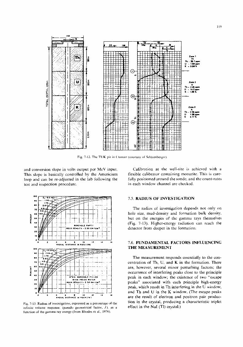
I19
I T
Fig. 7-12. The T U K pit in Clamart (courtesy of Schlumberger).
and conversion slope in volts output per MeV input. This slope is basically controlled by the Americium loop and can be re-adjusted in the lab following the test and inspection procedure.
Calibration at the well-site is achieved with a flexible calibrator containing monazite. This is care- fully positioned around the sonde, and the count-rates in each window channel are checked.
c I u 0
i
100
90
a 0
10
S O
SO
4 0
>O
2 0
10
0 0 2 4 6 a 10 I 2 I 4 I6
R A D l 4 L D I S T A N C E IN ROCK l l W
J 2 4 6 10 12 I , I.
R L D I A L D l S T 4 M C L I N R O C N { I M 1
Fig. 7-13. Radius of investigation, expressed as a percentage of the infinite volume response, (pseudo geometrical factor, J ) , as a function of the gamma ray energy (from Rhodes et al., 1976).
7.5. RADIUS OF INVESTIGATION
The radius of investigation depends not only on hole size, mud-density and formation bulk density, but on the energies of the gamma rays themselves (Fig. 7- 13). Higher-energy radiation can reach the detector from deeper in the formation.
7.6. FUNDAMENTAL FACTORS INFLUENCING THE MEASUREMENT
The measurement responds essentially to the con- centration of Th, U, and K in the formation. There are, however, several minor perturbing factors; the occurrence of interfering peaks close to the principle peak in each window; the existence of two “escape peaks” associated with each principle hgh-energy peak, which result in Th interfering in the U window, and Th and U in the K window. (The escape peaks are the result of electron and positron pair produc- tion in the crystal, producing a characteristic triplet effect in the NaI (Tl) crystal.)
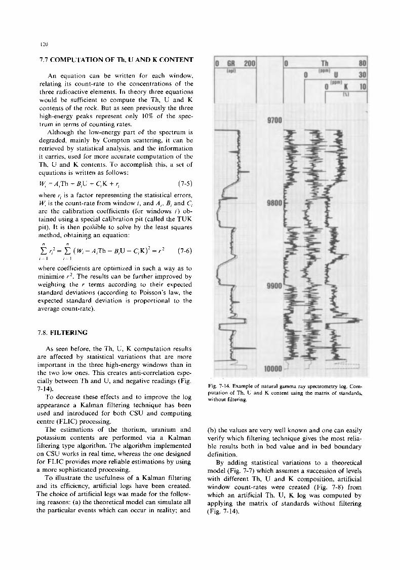
120
7.7 COMPUTATION OF Th, U AND K CONTENT
An equation can be written for each window, relating its count-rate to the concentrations of the three radioactive elements. In theory three equations would be sufficient to compute the Th, U and K contents of the rock. But as seen previously the three high-energy peaks represent only 10% of the spec- trum in terms of counting rates.
Although the low-energy part of the spectrum is degraded, mainly by Compton scattering, it can be retrieved by statistical analysis, and the information i t carries, used for more accurate computation of the Th, U and K contents. To accomplish this, a set of equations is written as follows:
w = A,Th + B,U + C,K + r, (7-5)
where r, is a factor representing the statistical errors, fl is the count-rate from window i, and A , , B, and C, are the calibration coefficients (for windows i ) ob- tained using a special calibration pit (called the TUK pit). It is then pos'sible to solve by the least squares method, obtainiqg an equation:
c r,2 = c (q - A,Th - B,U - C,K)2 = r 2 n n
(7-6)
where coefficients are optimized in such a way as to minimize r 2 . The results can be further improved by weighting the r terms according to their expected standard deviations (according to Poisson's law, the expected standard deviation is proportional to the average count-rate).
I = 1 I = 1
7.8. FILTERING
As seen before, the Th, U, K computation results are affected by statistical variations that are more important in the three high-energy windows than in the two low ones. This creates anti-correlation espe- cially between Th and U, and negative readings (Fig. 7- 14).
To decrease these effects and to improve the log appearance a Kalman filtering technique has been used and introduced for both CSU and computing centre (FLIC) processing.
The estimations of the thorium, uranium and potassium contents are performed via a Kalman filtering type algorithm. The algorithm implemented on CSU works in real time, whereas the one designed for FLIC provides more reliable estimations by using a more sophisticated processing.
To illustrate the usefulness of a Kalman filtering and its efficiency, artificial logs have been created. The choice of artificial logs was made for the follow- ing reasons: (a) the theoretical model can simulate all the particular events which can occur in reality; and
1
9700
Fig. 7-14. Example of natural gamma ray spectrometry log. Com- putation of Th, U and K content using the matrix of standards, without filtering.
(b) the values are very well known and one can easily verify which filtering technique gives the most relia- ble results both in bed value and in bed boundary definition.
By adding statistical variations to a theoretical model (Fig. 7-7) which assumes a succession of levels with different Th, U and K composition, artificial window count-rates were created (Fig. 7-8) from which an artificial Th, U, K log was computed by applying the matrix of standards without filtering (Fig. 7-14).
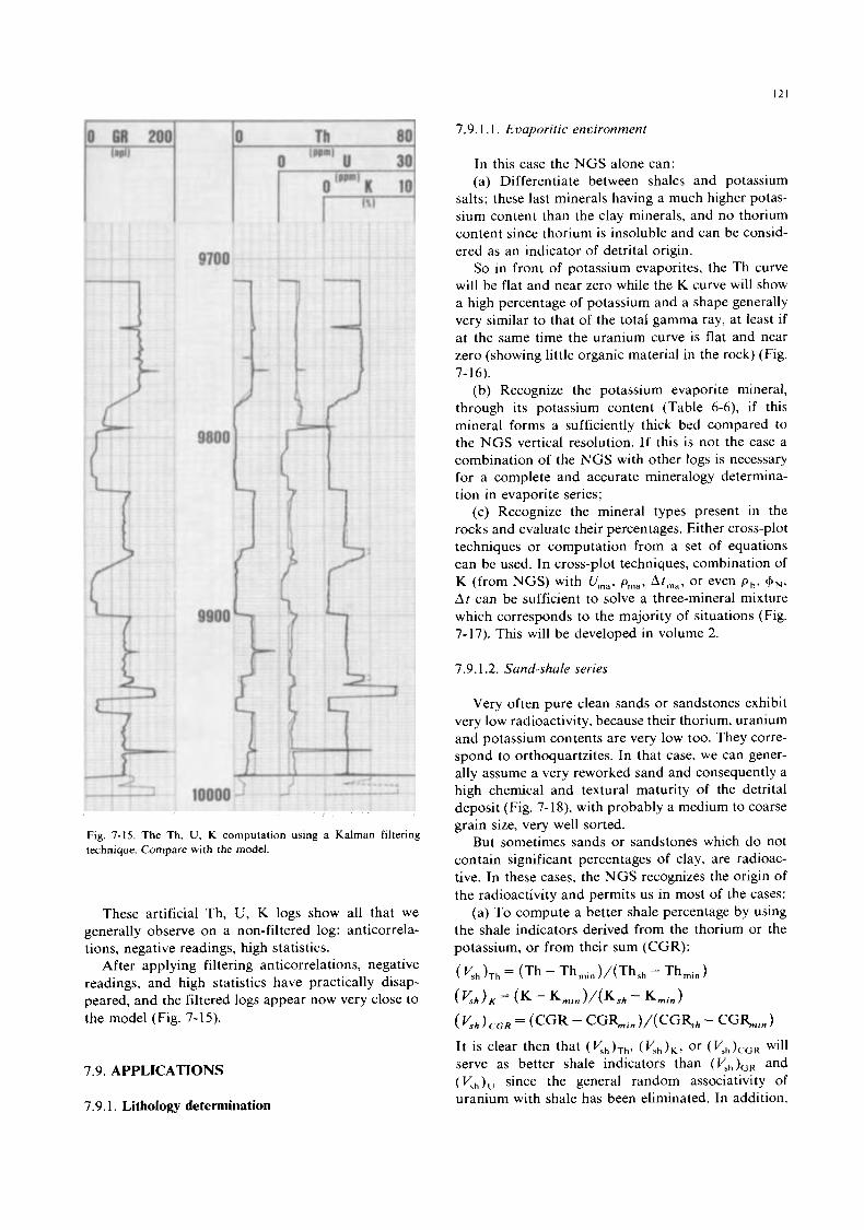
121
i '"7
Fig. 7-15. The Th, U, K computation using a Kalman filtering technique. Compare with the model.
These artificial Th, U, K logs show all that we generally observe on a non-filtered log: anticorrela- tions, negative readings, high statistics.
After applying filtering anticorrelations, negative readings, and high statistics have practically disap- peared, and the filtered logs appear now very close to the model (Fig. 7- 15).
7.9. APPLICATIONS
7.9.1. Lithology determination
7.9.1.1. Evuporitic environment
In this case the NGS alone can: (a) Differentiate between shales and potassium
salts; these last minerals having a much higher potas- sium content than the clay minerals, and no thorium content since thorium is insoluble and can be consid- ered as an indicator of detrital origin.
So in front of potassium evaporites, the Th curve will be flat and near zero while the K curve will show a high percentage of potassium and a shape generally very similar to that of the total gamma ray, at least if at the same time the uranium curve is flat and near zero (showing little organic material in the rock) (Fig.
(b) Recognize the potassium evaporite mineral, through its potassium content (Table 6-6), if this mineral forms a sufficiently thick bed compared to the NGS vertical resolution. If this is not the case a combination of the NGS with other logs is necessary for a complete and accurate mineralogy determina- tion in evaporite series;
(c) Recognize the mineral types present in the rocks and evaluate their percentages. Either cross-plot techniques or computation from a set of equations can be used. In cross-plot techniques, combination of K (from NGS) with Urn,, pma, At,,, or even ph? $J,.,, A t can be sufficient to solve a three-mineral mixture which corresponds to the majority of situations (Fig. 7- 17). This will be developed in volume 2.
7- 16).
7.9.1.2. Sand-shale series
Very often pure clean sands or sandstones exhibit very low radioactivity, because their thorium, uranium and potassium contents are very low too. They corre- spond to orthoquartzites. In that case, we can gener- ally assume a very reworked sand and consequently a high chemical and textural maturity of the detrital deposit (Fig. 7- 18), with probably a medium to coarse grain size, very well sorted.
But sometimes sands or sandstones which do not contain significant percentages of clay, are radioac- tive. In these cases, the NGS recognizes the origin of the radioactivity and permits us in most of the cases:
(a) To compute a better shale percentage by using the shale indicators derived from the thorium or the potassium, or from their sum (CGR):
( <h > T h = (Th - Th mtn - Th min
( V s h ), = (K - K,,, ) / (Ksh - K,,,) (K,) CGR = (CGR - C G L , )/(CG%h - C G l L n ) It is clear then that ( yh)rh, ( < h ) K , or (V,,),,, will serve as better shale indicators than (yh)GR and (y,)" since the general random associativity of uranium with shale has been eliminated. In addition,
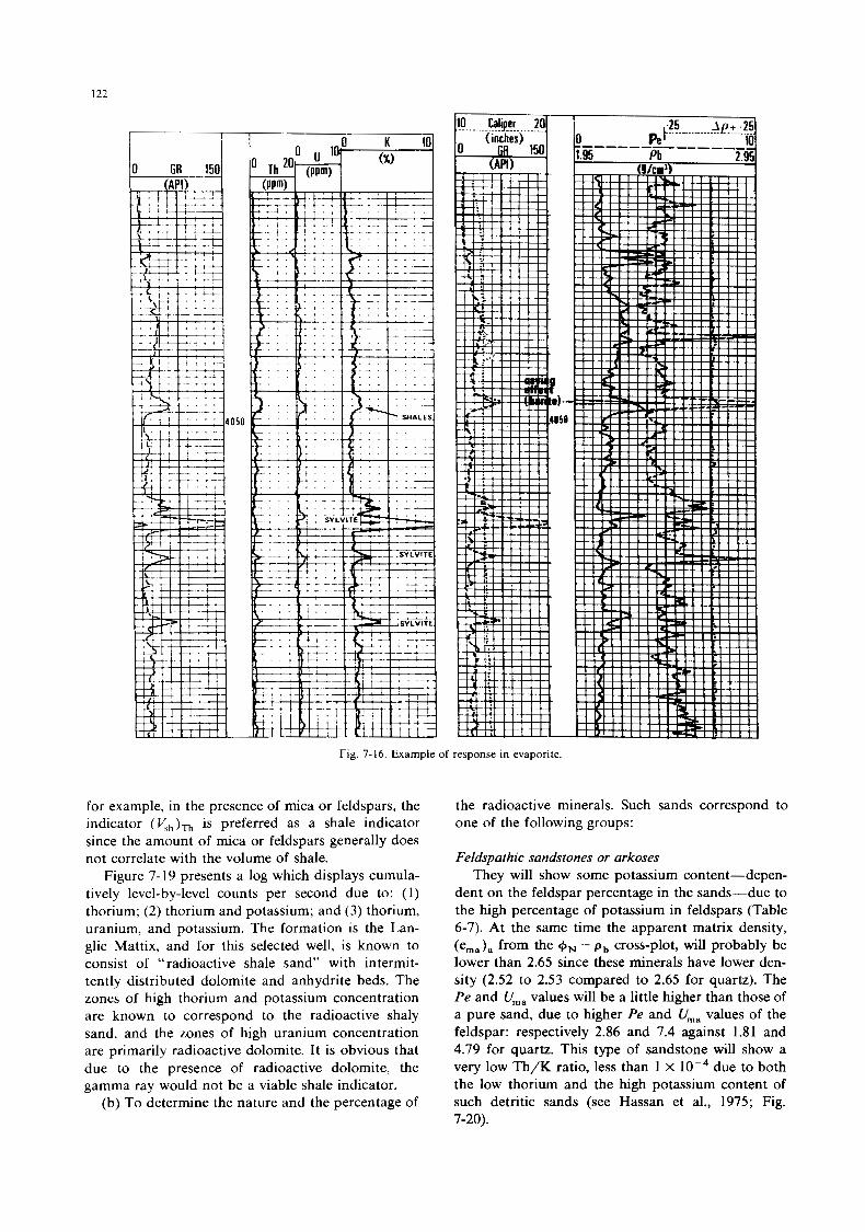
122
I i l I I I I I
Fig. 7-16. Example of response in evaporite.
for example, in the presence of mica or feldspars, the indicator (V,,),, is preferred as a shale indicator since the amount of mica or feldspars generally does not correlate with the volume of shale.
Figure 7-19 presents a log which displays cumula- tively level-by-level counts per second due to: (1) thorium; (2) thorium and potassium; and (3) thorium, uranium, and potassium. The formation is the Lan- glie Mattix, and for this selected well, is known to consist of “radioactive shale sand” with intermit- tently distributed dolomite and anhydrite beds. The zones of high thorium and potassium concentration are known to correspond to the radioactive shaly sand, and the zones of high uranium concentration are primarily radioactive dolomite. It is obvious that due to the presence of radioactive dolomite, the gamma ray would not be a viable shale indicator.
(b) To determine the nature and the percentage of
the radioactive minerals. Such sands correspond to one of the following groups:
Feldspathic sanhtones or arkoses They will show some potassium content-depen-
dent on the feldspar percentage in the sands-due to the high percentage of potassium in feldspars (Table 6-7). At the same time the apparent matrix density, (ema)a from the +N - p b cross-plot, will probably be lower than 2.65 since these minerals have lower den- sity (2.52 to 2.53 compared to 2.65 for quartz). The Pe and Urn, values will be a little higher than those of a pure sand, due to higher Pe and Urn, values of the feldspar: respectively 2.86 and 7.4 against 1.81 and 4.79 for quartz. This type of sandstone will show a very low Th/K ratio, less than 1 X lop4 due to both the low thorium and the high potassium content of such detritic sands (see Hassan et al., 1975; Fig. 7-20).
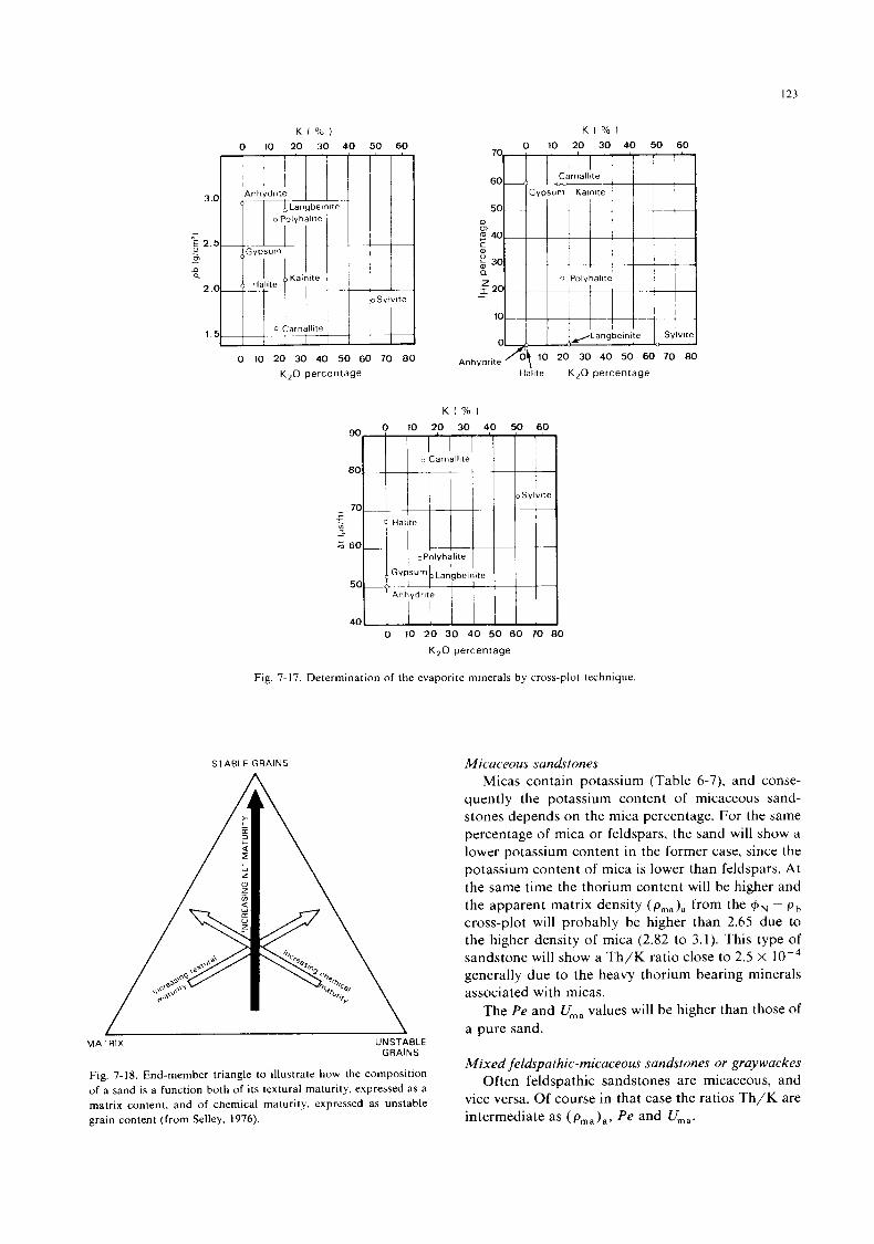
I23
K '10 1 K ( % ) 0 10 20 30 4 0 50 60 0 10 20 30 40 50 60
0 10 20 30 40 50 60 70 80 Anhydrite A' lo K,O percentage H a h e
20 30 40 50 60 70 80
K,O percentage
0 10 20 30 4 0 50 60 70 80
K,O percentage
Fig. 7- 17. Determination of the evaporite minerals by cross-plot technique.
STABLE G R A I N S
MATRIX U N S T A B L E G R A I N S
Fig. 7-18. End-member triangle to illustrate how the composition of a sand is a function both of its textural maturity, expressed as a matrix content, and of chemical maturity. expressed as unstable grain content (from Selley. 1976).
Micaceous sandstones Micas contain potassium (Table 6-7), and conse-
quently the potassium content of micaceous sand- stones depends on the mica percentage. For the same percentage of mica or feldspars, the sand will show a lower potassium content in the former case, since the potassium content of mica is lower than feldspars. At the same time the thorium content will be higher and the apparent matrix density (p, , ) , from the + N - p,, cross-plot will probably be higher than 2.65 due to the higher density of mica (2.82 to 3.1). This type of sandstone will show a Th/K ratio close to 2.5 X
generally due to the heavy thorium bearing minerals associated with micas.
The Pe and Urn, values will be higher than those of a pure sand.
Mixed feldspathic-micaceous sandstones or graywackes Often feldspathic sandstones are micaceous, and
vice versa. Of course in that case the ratios Th/K are intermediate as (p, , ) , , Pe and U,,.
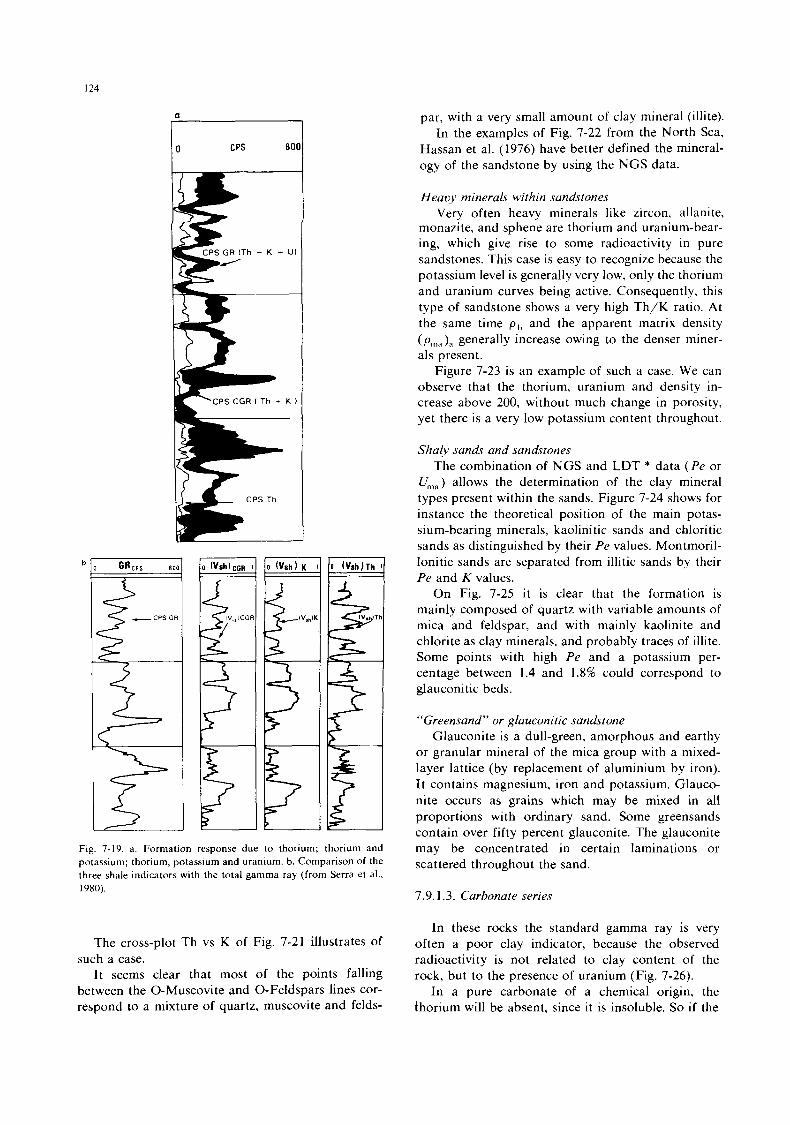
124
b
- CPS GR F
Th + K + U)
Fig. 7-19. a. Formation response due to thorium; thorium and potassium; thorium, potassium and uranium. b. Comparison of the three shale indicators with the total gamma ray (from Serra et al., iyno).
The cross-plot Th vs K of Fig. 7-21 illustrates of such a case.
It seems clear that most of the points falling between the 0-Muscovite and 0-Feldspars lines cor- respond to a mixture of quartz, muscovite and felds-
par, with a very small amount of clay mineral (illite). In the examples of Fig. 7-22 from the North Sea,
Hassan et al. (1976) have better defined the mineral- ogy of the sandstone by using the NGS data.
Heavy minerals within sandstones Very often heavy minerals like zircon, allanite,
monazite, and sphene are thorium and uranium-bear- ing, which give rise to some radioactivity in pure sandstones. This case is easy to recognize because the potassium level is generally very low, only the thorium and uranium curves being active. Consequently, this type of sandstone shows a very high Th/K ratio. At the same time ph and the apparent matrix density ( p,,), generally increase owing to the denser miner- als present.
Figure 7-23 is an example of such a case. We can observe that the thorium, uranium and density in- crease above 200, without much change in porosity, yet there is a very low potassium content throughout.
Shaly sands and sandstones The combination of NGS and LDT * data ( P e or
U,,) allows the determination of the clay mineral types present within the sands. Figure 7-24 shows for instance the theoretical position of the main potas- sium-bearing minerals, kaolinitic sands and chloritic sands as distinguished by their Pe values. Montmoril- lonitic sands are separated from illitic sands by their Pe and K values.
On Fig. 7-25 i t is clear that the formation is mainly composed of quartz with variable amounts of mica and feldspar, and with mainly kaolinite and chlorite as clay minerals, and probably traces of illite. Some points with high Pe and a potassium per- centage between 1.4 and 1.8% could correspond to glauconitic beds.
“Greensand” or glauconitic sandstone Glauconite is a dull-green, amorphous and earthy
or granular mineral of the mica group with a mixed- layer lattice (by replacement of aluminium by iron). It contains magnesium, iron and potassium. Glauco- nite occurs as grains which may be mixed in all proportions with ordinary sand. Some greensands contain over fifty percent glauconite. The glauconite may be concentrated in certain laminations or scattered throughout the sand.
7.9.1.3. Carbonate series
In these rocks the standard gamma ray is very often a poor clay indicator, because the observed radioactivity is not related to clay content of the rock, but to the presence of uranium (Fig. 7-26).
In a pure carbonate of a chemical origin, the thorium will be absent, since it is insoluble. So if the
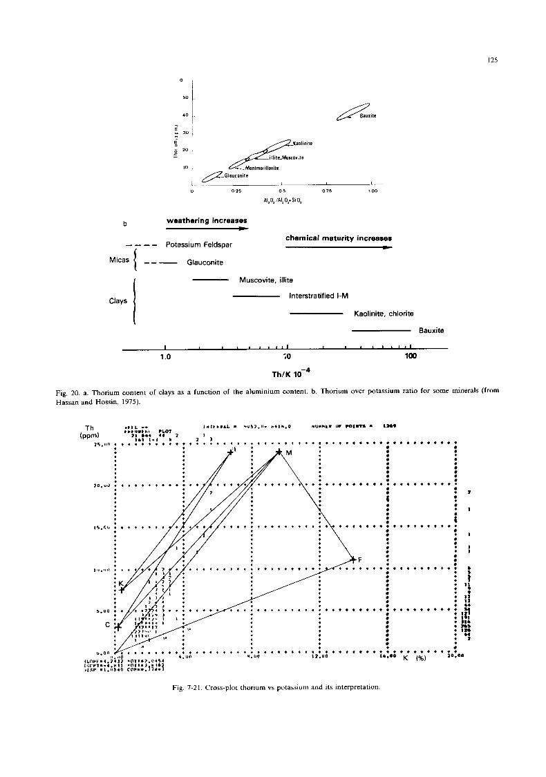
125
auxitc
0 0 25 0 5 0 7 5 100
AI,O,/AI,O,+SIO,
weathering increases b t
- - - - Potassium Feldspar
Glauconite
chemical maturity increases t
Clays
Muscovite, illite
lnterstratified I-M
Kaolinite, chlorite
Bauxite
I 1 I 1 I I I I I I 1 I I I
1 .o i 0 100
Th/K
Fig. 20. a. Thorium content of clays as a function of the aluminium content. b. Thorium over potassium ratio for some minerals (from Hassan and Hossin, 1975).
* * * * * * * * * *
t
. .
t
* . * . * * . * * *
. * * * . * * * * *
* . * * * * * * * *
* * * * * . * * * *
* * * * * * * * * t lb.00 K (%)
* . . + *
* l . . * l
* * * I
* I * l
1. * : ; : r .
* * 20.00
Fig. 7-2 1. Cross-plot thorium vs potassium and its Interpretation.
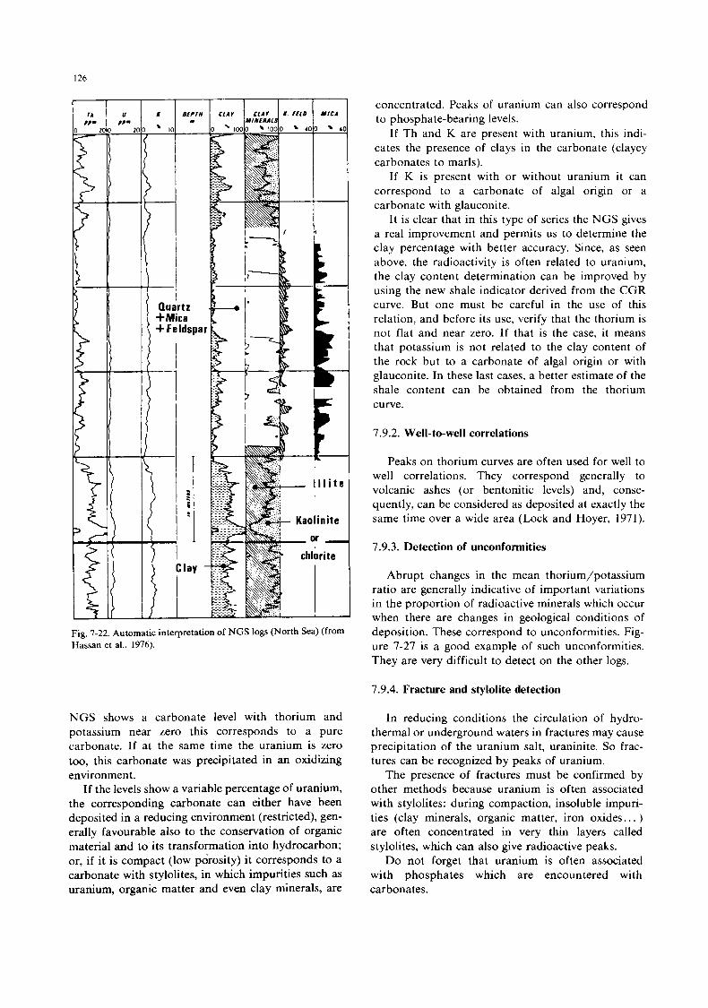
126
Fig. 7-22. Automatic interpretation of NGS logs (North Sea) (from Hassan et al., 1976).
NGS shows a carbonate level with thorium and potassium near zero this corresponds to a pure carbonate. If at the same time the uranium is zero too, this carbonate was precipitated in an oxidizing environment.
If the levels show a variable percentage of uranium, the corresponding carbonate can either have been deposited in a reducing environment (restricted), gen- erally favourable also to the conservation of organic material and to its transformation into hydrocarbon; or, if it is compact (low porosity) it corresponds to a carbonate with stylolites, in which impurities such as uranium, organic matter and even clay minerals, are
concentrated. Peaks of uranium can also correspond to phosphate-bearing levels.
If Th and K are present with uranium, this indi- cates the presence of clays in the carbonate (clayey carbonates to marls).
If K is present with or without uranium it can correspond to a carbonate of algal origin or a carbonate with glauconite.
It is clear that in this type of series the NGS gives a real improvement and permits us to determine the clay percentage with better accuracy. Since, as seen above, the radioactivity is often related to uranium, the clay content determination can be improved by using the new shale indicator derived from the CGR curve. But one must be careful in the use of this relation, and before its use, verify that the thorium is not flat and near zero. If that is the case, it means that potassium is not related to the clay content of the rock but to a carbonate of algal origin or with glauconite. In these last cases, a better estimate of the shale content can be obtained from the thorium curve.
7.9.2. Well-to-well correlations
Peaks on thorium curves are often used for well to well correlations. They correspond generally to volcanic ashes (or bentonitic levels) and, conse- quently, can be considered as deposited at exactly the same time over a wide area (Lock and Hoyer, 1971).
7.9.3. Detection of unconformities
Abrupt changes in the mean thorium/potassium ratio are generally indicative of important variations in the proportion of radioactive minerals which occur when there are changes in geological conditions of deposition. These correspond to unconformities. Fig- ure 7-27 is a good example of such unconformities. They are very difficult to detect on the other logs.
7.9.4. Fracture and stylolite detection
In reducing conditions the circulation of hydro- thermal or underground waters in fractures may cause precipitation of the uranium salt, uraninite. So frac- tures can be recognized by peaks of uranium.
The presence of fractures must be confirmed by other methods because uranium is often associated with stylolites: during compaction, insoluble impuri- ties (clay minerals, organic matter, iron oxides. . . ) are often concentrated in very thin layers called stylolites, which can also give radioactive peaks.
Do not forget that uranium is often associated with phosphates which are encountered with carbonates.
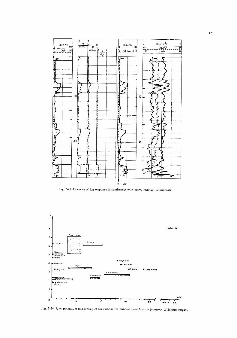
321s 118
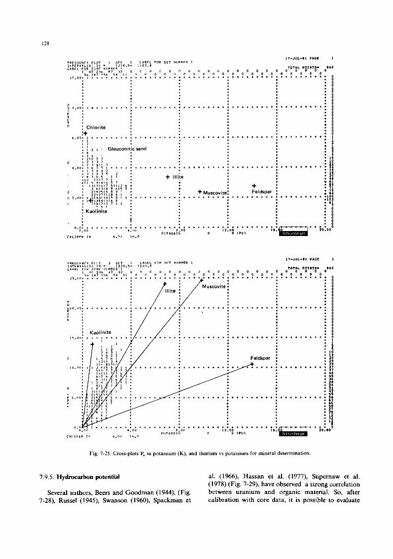
128
FRFOUENCY PLOT 1 SFT I 1,A4FL, I N T E P V b L ( S 1 I N u 1 2 3 4 . 5 - 1 1 0 3 . 4 L A B F l , FOR ZONF MllMRFR 1
I B O 7 3 b 0 7 32 0 0 0 5 6 1 4 7 1 5 6 5 4 1 1 n n
i n . o o + + + t + t + + + + + + t + t + +
F O R S E T N U Y R F R 1 17-JUL-I1 PACE I
TOTAL POIIITSS 860 0 0 0 0 0 0 0 0
0 0 0 0 0 0 0 0 + + + + + + + + + t + + + + + t 0 t o
0 0 0 0 0 0 0 0
* + + + t * t t
0 0
+ + * 0
+ t + t + + t + t
+ + + +
+ + t t t * + +
+ + + + +
t
+ + +
+ o t + o + t + * . + t + t t t 0 t + o
+ + P t e 0 . 0 0 * t + + + + + + + + + + + - + +
C t T t + i : +
:+ + ” : Chlorite +
6.00, I + + + + t t + + + + + t t t l + r 2 + + I + I 2 1 I Glauconitic sand I ”
+
+ + + + * + + *
+ + + t
t
+ + + + +
+ t + + + t t *
+ + + t + + + * +
t + + + +
t t + t t +
+ + + + + + + t + t + t +
+ + + + + t
+ + + + + + + +
t + t + + + + + + + + + t + +
t 9 + 16
+ t , + t + t t i 11 + 14 + 1s + 2 0 + 4 0
61
+ 19 ‘94
r * + + + . + * t l O 5 +lo3
: J :
: ‘4
v 4 * + , + * * +
2 + I *
l t 1 1 2 b t 6 1 5 5 t 9 1 + 4 1 + 5 1 * t + * * U t 1 2 t
+ + + t * + + + *
+ ;
t + t + + * t t + + t + t
+
+ + . t +
+ I H i &
+ +
t + + t + + t t t t + + + + + + +
+ Feldspar * t + + +
t Muscovite: + + t + + + t *
t + + t + + + +
+ + + + + + + + + +
+ 1 5 1 t t + +
+ + t
: Kaolinite
3, +
o.n+ t + t + + t t + + + t t t t 0 . 0 0 4.130
C A L I P F R I N 6 . 0 1 Ib.0
+ t o + + + * o * o t o t o i n
+ + t t + + + t t
12.00 0
+ + + IPUI
+ + + ; 6 2 0 . 0 0
+ * + + + t 16.
t + + + t + t + @.no
POT ASS I IJ
17-JUL-81 PACE 3 PRFUIIFNCY PI117 2 S k T 1 L b t l t L FflR S F T NI IMPER I
I N T k R V b I . ( F l I N - 1 2 3 4 . 5 - 1 1 0 3 . 4 TOTAL POINTS= 0 6 0 LACIFL FL lU ZONF hUMRFR 1
* + + + + + + + + * 0 t o t + o + t o + + o . + o t t o t t o
t o t o
+ + + + + + + * + + 0 + o + o r o
+ t * o t + o
t + + * o + + + + o
+ + t o + o + + + + + + * + + + 0
+ I t + + I + t t 2 + + I + + 10
+ 12 + PO t 1 9 + 39
+ t + + + + t t t 37 + 31 + 46 t 45 t 36 + 28 t 24 t 21
+ + 41 + 59 + + + + + + + + t t $6
t + + 63 + + 66 + + 59 t + + 1 7 t + + 28 + + + 12 + + t 32
-tt+ + t t 3
1 f l n 2 1 h k 1 7 3 2 0 n 0 0 0 n 0 0 0 0 0 0 0 0 0 0 0 0 0 0 0 5 0 1 4 7 i 5 6 5 4 1 1 n n o n n 0 n 0 0 0 0 0 0 0 0 0 0 0 0 0
+ +
20.00 P l i T A S S l I1 n
CAI IPtP I ) b.01 16.0
Fig. 7-25. Cross-plots Pe vs potassium (K), and thorium vs potassium for mineral determination.
7.9.5. Hydrocarbon potential al. (1966), Hassan et al. (1977), Supernaw et al. (1978) (Fig. 7-29), have observed a strong correlation between uranium and organic material. So, after calibration with core data, it is possible to evaluate
Several authors, Beers and Goodman (1944), (Fig. 7-28), Russel (1945), Swanson (1960), Spackman et
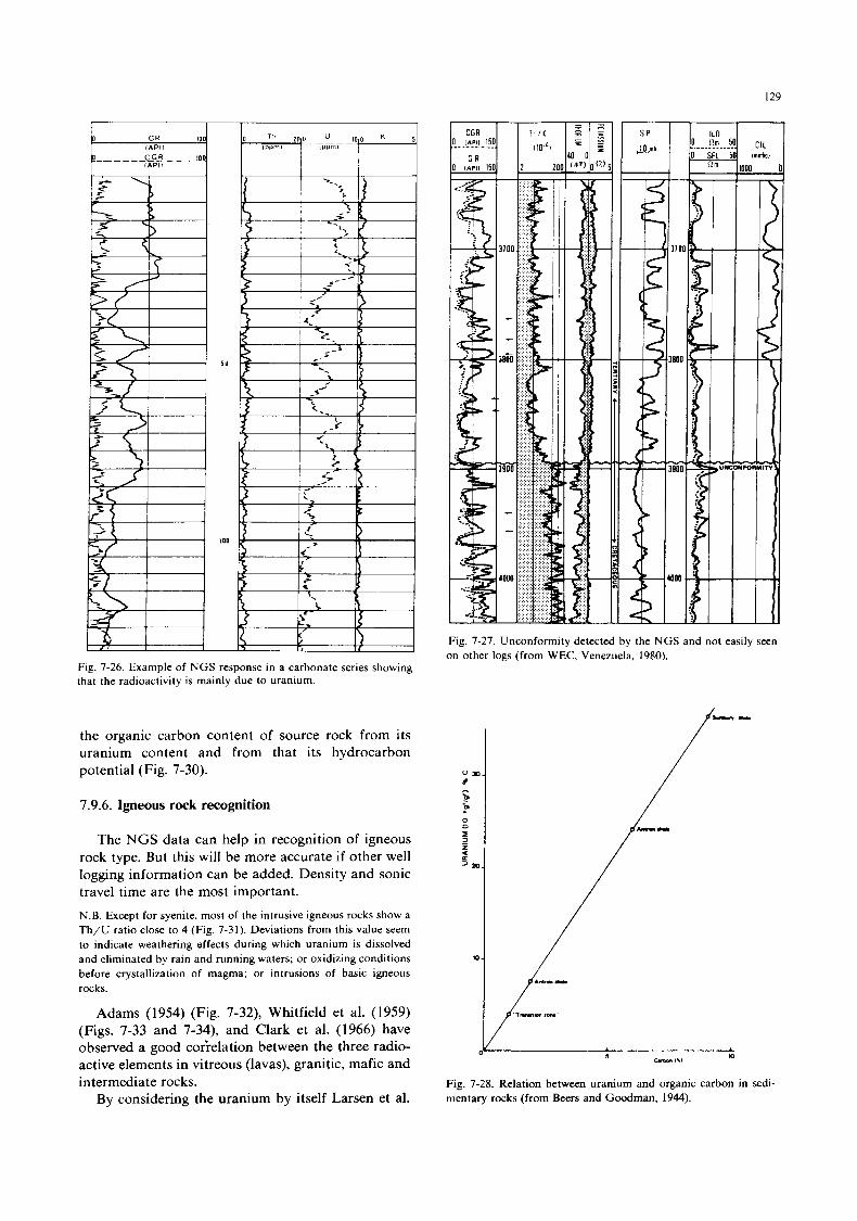
Fig. 7-26. Example of NGS response in a carbonate series showing that the radioactivity is mainly due to uranium.
the organic carbon content of source rock from its uranium content and from that its hydrocarbon potential (Fig. 7-30).
7.9.6. Igneous rock recognition
The NGS data can help in recognition of igneous rock type. But this will be more accurate if other well logging information can be added. Density and sonic travel time are the most important. N.B. Except for syenite, most of the intrusive igneous rocks show a Th/U ratio close to 4 (Fig. 7-31). Deviations from this value seem to indicate weathering effects during which uranium is dissolved and eliminated by rain and running waters; or oxidizing conditions before crystallization of magma; or intrusions of basic igneous rocks.
Adams (1954) (Fig. 7-32), Whitfield et al. (1959) (Figs. 7-33 and 7-34), and Clark et al. (1966) have observed a good coirelation between the three radio- active elements in vitreous (lavas), granitic, mafic and intermediate rocks.
By considering the uranium by itself Larsen et al.
Fig. 7-27. Unconformity detected by the NGS and not easily seen on other logs (from WEC, Venezuela, 1980).
I
30. f - D
D
0 5
f < c m.
5 L
c-.a ,\I 0
Fig. 7-28. Relation between uranium and organic carbon in sedi- mentary rocks (from Beers and Goodman, 1944).
130
0.9
0.0
- 0.7 a
u 5
0.6
s 2 0.5 4
$ 0.4 3 z 2 0.3 3
+
-
0.2
0.1
0
URANIUM POOTISSKIY P A 1 0
ORGANIC C U I W N
(NEW 41-V WALE1
r = 0 9 7 5
Fig. 7-29. Relation between uranium and organic carbon (from Supernaw et al., 1978).
(1954) have found a good correlation between the uranium content and the igneous type rocks (Fig. 7-35).
7.9.7. Sedimentology
Through the information on the radioactive ele- ments present in the rocks, the NGS is a very power- ful tool for sedimentological applications.
The recognition of radioactive minerals, especially of the clay minerals present in the rocks, and an
Th = 1300 I U = 2500 SYENITE
I I . GRANITE
a GRANOOIORITE
.
5 m 15 20 UIWrnl
Fig. 7-31. Thorium vs uranium cross-plot for the main igneous rocks.
understanding of the conditions of deposition through the uranium measurement (oxidizing if free of uranium, reducing if rich in uranium), give a better determination of the mineralogical and grain size vertical distribution, and allow a more accurate re- construction of the depositional environment. These are often characterized by the presence of certain minerals (Hassan et al., 1976) (Table 7-1):
(a) Glauconite is of marine origin, forming mainly in continental shelf conditions.
(b) Phosphatic deposits occur in similar condi- tions, but with the added requirements of warm water and a reducing environment.
(c) Feldspars are indicators of the degree of evolu- tion of sand facies. Being unstable, they will only be
0300 - I- z w 0
w a n.
5 .0200 - r' 2 a a 3
0 25 50 75 100 0 25 50 75
TOTAL ORGANIC MATTER IN ROCK, IN PERCENT TOTAL ORGANIC MATTER IN ROCK, I N PERCENT
Fig. 7-30. Diagrams showing possible relation of uranium content to oil yield of a marine black shale, as controlled by total organic matter and the proportions of humic and sapropelic material making up the organic matter (from Swanson, 1960).
131
10
8 -
URANIUM AND THORIUM CONTENT VERSUS THE POTASSIUM FELDSPAR/PLAGIOCLASE
RATIO OF GRANITIC ROCKS
- .URANIUM CONTENT
Uranium content, (pprn)
Fig. 7-32. Relation between potassium and uranium content of rocks in the Larsen Peak region, California (from Adams, 1954).
found relatively close to the source rocks.
oped continental environment with good drainage.
tional environments.
tions.
(d) Bauxite forms in a warm, humid, well-devel-
(e) Clay typing is widely used in analyzing deposi-
(f) Uranium indicates low-energy, reducing condi-
7.9.8. Diagenesis
Diagenesis causes the alteration of clay minerals (montmorillonite, illite, mixed layer I-M), the disap- pearance of kaolinite (which is transformed into il- lite), or a neogenesis in sands (kaolinite). These phe- nomena can be studied from gamma-ray spectrome- try and, in particular, the Th/K ratio.
Under compaction, montmorillonite is trans-
URANIUM AND POTASSIUM V E R S U S THORIUM CONTENT IN GRANITIC ROCKS t
0 1 5 10 15 2 5 2 0
THORIUM, T h ( pprn)
Fig. 7-33. Uranium and potassium vs thorium content in granitic rocks (after data from Whitfield et al., 1959).
I ’ 311
2 4 6 (0 20 40 60 100 URANIUM 1U1 AND THORIUM ‘Tni,ppm
Fig. 7-34. Uranium and thorium content vs Potassium feldspar/plagioclase ratio of granitic rocks (after data from Whit- field et al., 1959).
COMPOSITION OF ROCKS, 113 SoO, + K,O-FeO-MgO-CaO Qtr OlORlTE GRANODIORITE GRANITE GABBRO
Fig. 7-35. Distribution of uranium in rocks of the southern Cali- fornia Batholith plotted as a function of the composition of the rocks (from Larsen et al., 1954).
TABLE 7-1
Thorium and uranium content of clay minerals (data from Adams and Weaver, 1958; Clark et al., 1966; Hassan et al., 1975)
Minerals Th (PPm) u (PPm)
Illite 10- 25 1.5 Montmonllonite 10- 24 2 - 5 Bentonite 4- 55 1 -36 Kaolinite 6- 42 1.5- 9 Chlorite 3- 5 Glauconite < 10 Bauxite 10-132 3 -30
132
formed into illite, passing through an intermediate mixed-layer illite-montmorillonite phase (Hassan et al., 1976). This results in a decrease of the Th/K ratio with depth. In undercompacted shales this trend will be reversed.
In carbonate reservoirs, diagenesis strongly affects the concentration and distribution of uranium (Has- san et al., 1976): (a) uranium can be easily mobilized and migrates during leaching and dissolution; (b) a high uranium concentration is characteristic of material filling or surrounding stylolites (Hassan et al., 1976); and (c) phosphatization in carbonates, too, results in a build-up of uranium (Hassan and Al- Maleh, 1976).
7.9.9. Estimation of the uranium potential
Natural gamma-ray spectrometry allows the direct estimation of the uranium content of the rocks, and consequently the detection of the uranium ores.
7.9.10. An approach to the cation exchange capacity
From the fact that one can define the type and the percentage of the clays present in the rocks, one can compute a parameter related to the cation exchange capacity.
7.9.1 1. Radioactive scaling
Abnormally high uranium content is frequently observed in front of perforated intervals in old wells. This is due to the precipitation of radioactive salts (radio-barite, Ba( Ra)SO,).
Under dynamic conditions, radium isotopes are transported through permeable reservoirs, during the primary production of a water-flood operation, until final precipitation occurs at perforated (or around unperforated) cased wellbores. This precipitation de- pends on variations in temperature, pressure, flow and chemical equilibrium.
7.10. ENVIRONMENTAL AND OTHER EFFECTS
7.10.1. Time constant (vertical smoothing), logging speed, dead time
These are discussed in Chapter 5.
7.10.2. The bore-hole
The bore-hole influence is essentially due to ab- sorption and Compton scattering. These are a func- tion of several factors:
(a) Energy of the gamma rays emitted: the absorp- tion is higher when the gamma energy is lower (Fig. 7-36).
SILICON
100
C ._ c
L
51 n Q
0.1
Fig. 7-36. The Compton scattering and photoelectric absorption increase when the gamma energy decreases (from Adam and Gasparini, 1970).
(b) Volume of the bore-hole fluid around the tool which depends on the diameters of the hole and the tool.
5 1 b P 4
0 1
0 01 01 1
Gamma r.v ENERGY E IMcVl
Fig. 7-37. Compton Scattemg and photoelectnc absorption as a function of density and atomc number (from Adams and Gaspanni, 1970).
133
(c) Nature of the bore-hole fluid. ( 1 ) Its density (air, gas, water, oil): the Compton
scattering is higher when the density is higher; (2) Its effective atomic number Z; the absorp-
tion will be higher if its content of strong gamma absorbers like barite is higher (Fig. 7-37).
(3) Its content of radioactive materials: be- ntonite, potassium salts (e.g. KCl mud), etc.
7.10.3. Tool position
Tool excentering is a departure from the idealized concentrically cylindrical geometry and the log read- ings are affected accordingly.
7.10.4. Casing
In cased hole the nature of the casing-its thck- ness, its position in the hole, and the nature and the volume of the cement between the casing and the formation-all contribute to absorption and Comp- ton scattering, preferentially attenuating the low-en- ergy gamma rays. The measured spectrum is thus unfairly weighted towards the high energies.
7.10.5. Bed thickness
As for other radioactive techniques, the log read- ings in a thin bed depend on the thickness of the bed, and the volume it represents relative to the spheres of influence of the three radioactive elements.
Rhodes et al. (1966) proposed correction charts for these effects. However, they are somewhat difficult to apply.
7.1 1 REFERENCES
Adams, J.A.S., 1954. Uranium and thorium contents of volcanic rocks. In: Nuclear Geology. J. Wiley & Sons, N.Y.
Adams, J.S. and Gasparini, P., 1970. Gamma ray spectrometry of rocks. Elsevier, Amsterdam.
Adams, J.S. and Weaver, C.E., 1958. Thorium to uranium ratio as indicator of sedimentary processes: examples of concept of geochemical facies. Bull. Am. Assoc. Pet. Geol., 42 (2).
Baleine, O., Charlet, J.M., Dupuis, Ch. and Meys, H. (1976). Dosage par spectrometrie des radidlements naturels. Appli- cation A I'etude de quelques formations du bassin de Mons. Ann. Sci. DCpt. Mines-Ghlogie, Fac. Polytech. Mons, 2.
Beers, R.F. and Goodman, C., 1944. Distribution of radioactivity in ancient sediments. Bull. Geol. Soc. America, 55.
Bell, K.G., 1954. Uranium and thorium in sedimentary rocks. In: Nuclear Geology. J. Wiley & Sons, N.Y.
Blatt, H., Middleton, G. and Murray, R., 1980. Origin of Sedimen- tary Rocks (2nd 4.). Prentice-Hall, E n g l e w d Cliffs, N.J.
Brannon, Jr, H.R. and Osoba, J.S., 1956. Spectral gamma ray logging. Trans. AIME, 207.
Caillere, S. and Henin, S., 1963. Mineralogie des Argiles. Masson & Cie., Paris.
Civetta, L., Gasparini, P. and Adams, J.A.S., 1965. Aspetti dell'
evoluzione magmatica del vulcano di Roccamonfina attraverso misure di radioattivita. Ann. Osserv. Vesuviano, Vol. 7.
Clark, S.P.Jr, Peterman, Z.E. and Heier, K.S., 1966. Abundances of uranium, thorium and potassium. Handbook of Physical Con- stants, 1966.
Cody, R.D., 1971. Absorption and the Reliability of Trace Ele- ments as Environment Indicators for Shales. J. Sediment. Pet., Vol. 41, No. 2.
Deer, W.A., Howie, R.A. and Zussman, J., 1978. Rock Forming Minerals (2nd Ed.) Halsted Press (6 Volumes).
Doig, 1968. The natural gamma-ray flux: in situ analysis. Geo- physics, 33 (2).
Dumesnil, P. and Andrieux, C., 1970. Spectrometrie gamma dans les forages par sonde a semi-conducteur Ge-Li. Revue In- dustries Atomiques, no 11/12.
Dunoyer De Segonzac, G., 1969. Les mineraux argileux dans la diagenese. Passage au metamorphisme. Mem. Serv. Cart. Geol. Als.-Lorr., 29.
Evans, R.D., 1955. The Atomic Nucleus. McGraw-Hill, N.Y. Fertl, W.H., 1979. Gamma ray spectral data assists in complex
formation evaluation. The Log Analyst, vol 20, No. 5. Fertl, W.H., Stapp, W.L., Vaello, D.B., and Vercellino, C., 1978.
Spectral Gamma Ray Logging in the Austin Chalk trend. SPE 7431, SPE of AIME, Fall Mtg., Houston, TEXAS, Oct. 1-3.
Fertl, W.H., Welker, D.W. and Hopkinson, E.C., 1978. The Dresser Atlas Spectralog-A look at basic principles, field applications and interpretive concepts of gamma ray spectral logging. Dresser Atlas Publication No. 3332, September.
Frost, E. Jr, and F e d , W.H., 1979. Integrated Core and Log analysis Concepts in Shaly Clastic Reservoirs. 7th Formation Evaluation Symp. of the Canadian Well Log. Society, Calgary.
Gasparini, P., Luongo, G. and Davia, G., 1963. Misure di radioat- tivita alla Solfatara di Pozzuoli. Atti Conv. Assoc. Geofis. Ital., 12, Rome, pp. 41-50.
Grim, R.E., 1958. Concept of diagenesis in argllaceous sediments. Bull. Am. Assoc. Pet. Geol., 42 (2).
Grim, R.E., 1968. Clay Mineralogy (2nd ed.). McGraw-Hill, New York, N.Y.
Hassan, M., 1973. The use of radioelements in diagenetic studies of shale and carbonate sediments. Int. Symp. Petrography of Organic Material in Sediment. Centre Nat. Rech. Sci., Pans, Sept. 1973.
Hassan, M. and Al-Maleh, K., 1976. La repartition de l'uranium dans les phosphates Senoniens dans le Nord-Ouest Syrien. C. R. Acad. Sci. (Pans), 282.
Hassan, M. and Hossin, A,, 1975. Contribution a l'etude des comportements du thorium et du potassium dans les roches sedimentaires. C.R. Acad. Sci. (Paris), 280.
Hassan, M., Selo, M. and Combaz, A., 1975. Uranium distribution and geochemistry as criteria of diagenesis in carbonate rocks. 9th Int. Sediment. Congr. (Nice, 1975), 7.
Hassan, M., Hossin, A. and Combaz, A., 1976. Fundamentals of the differential gamma-ray log. Interpretation technique. SPWLA. 17th Ann. Log. Symp. Trans., Paper H.
Hodson, G., Fertl, W.H. and Hammack, G.W., 1975. Formation Evaluation in Jurassic sandstones in the northern North Sea area. SPWLA, 16th Ann. Log. Symp. Trans., Paper 11.
Institut Franpis du Petrole (1963). La spectrornetrie du rayonne- ment nature1 des roches sementaires. Bureau d'Etudes Geologiques, Rapport no. 9000.
Keller, W.D., 1958. Argillaceous and direct bauxitization. Bull. Amer. Assoc. Petroleum Geol., 42, 2.
Keys, W.S., 1979. Borehole Geophysics in Igneous and Metamor- phic Rock. SPWLA, 20th Ann. Log. Symp. Trans., pap. 00.
King, R.L. and Bradley, R.W., 1977. Gamma-ray log finds bypassed oil zones in six Texas oilfields. Oil Gas J., April 4.
Krumbein, W.C. and Sloss, L.L., 1963. Stratigraphy and Sedimen- tation. W.H. Freeman & Co, San Francisco.
I34
Larsen, E.S., Jr., and Phair, G., 1954. The distribution of uranium and thorium in igneous rocks. In: Nuclear Geology. J. Wiley & Sons, New York.
Lock, G.A. and Hoyer, W.A., 1971. Natural gamma ray spectral Logging. The Log Analyst, 12 (5).
Luongo, G. and Rapolla, A., 1964. Contributo all0 studio dell’evoluzione del magma Somma-Vesuviano mediante le de- terminazione delle concentrazioni in isotopi radioattivi 238U, 232Th. 226Ta. e 40K. Ann. Osserv. Vesuviano, vol. 6.
Marett, G., Chevalier, P., Souhaite, P. and Suau, J., 1976. Shaly sand evaluation using gamma ray spectrometry applied to the North Sea Jurassic. SPWLA, 17th Ann. Log. Symp. Trans., Paper DD.
Millot, G., 1963. Geologie des Argiles. Masson & Cie., Pans. Millot, G.. 1963. Clay. Sci. Am., 240 (4). Moll, S.T., 1980. Spectral Gamma Logging in the Copper Moun-
tain Uranium Uistricf: A case Study in Fractured Quartz Monzonite. SPWLA, 21st Ann. Log. Symp. Trans., Paper 0.
Naidu, A.S., Burrel, D.C. and Hood, D.W., 1971. Clay mineral composition and geologic significance of some Beaufort Sea sediments. J. Sediment. Petrol., 41 (3).
Pettijohn, F.J., 1975. Sedimentary Rocks (3rd ed.). Harper & Row, New York.
Pettijohn, F.J., Potter, P.E. and Siever, R., 1972. Sand and Sand- stone. Springer-Verlag, Berlin.
Press, F. and Siever, R., 1978. Earth (2nd ed.). W.H. Freeman, San Francisco.
Quirein. J.A., Baldwin, J.L., Terry, R.L. and Hendrieks, M., 1981. Estimation of clay types and volumes from well log data. An extension of the global method. SPWLA, 22nd Ann. Log. Symp. Trans., Paper Q.
Rhodes, D.F. and Mott, W.E., 1966. Quantitative interpretation of gamma-ray spectral log. Geophysics, 3 1 (2).
Roubault, M., 1958. Geologie de I’uranium. Masson, Pans. Russell, W.L., 1945. Relation of Radioactivity, Organic content,
and sedimentation. Bull. Am. Assoc. Pet. Geol., 29 (10). Schenewerk, P.A., Sethi, D.K., F e d , W.H. and Lochmann, M.,
1980. Natural Gamma ray Spectral logging aids granite wash reservoir evaluation. SPWLA, 21st Ann. Log. Symp. Trans., Paper BB.
Schlumberger, 198 I . Natural Gamma-ray Spectrometry. Technical Book.
Schlumberger, 1982. Essentials of NGS interpretation Selley, R.C., 1976. An Introduction to Sedimentology. Academic
Press, London. Selley, R.C., 1978. Ancient Sedimentary Environments. (2nd Ed.).
Chapman & Hall, London. Serra, O., Baldwin, J. and Quirein, J., 1980. Theory, interpretation
and practical applications of Natural Gamma-ray Spectros- copy. SPWLA, 2lst Ann. Log. Symp. Trans., Paper Q.
Stromswold, D.C., 1980. Comparison of Scintillation Detectors for Borehole Gamma-ray logging. SPWLA, 21st Ann. Log. Symp. Trans., Paper EE.
Stromswold, D.C. and Kosanke, K.L., 1979. Spectral Gamma-ray logging I: Energy Stabilization Methods. SPWLA, 20th Ann. Log. Symp. Trans., Paper DD.
Suau, J. and Spurlin, J., 1982. Interpretation of micaceous sand- stones in the North Sea. SPWLA, 23rd Ann. Log. Symp. Trans., Paper G.
Supernaw, I.R., McCoy, A.D. and Link, A.J., 1978. Method for in-situ evaluation of the source rock potential of each forma- tion. U.S. PATENT 4,071,744, Jan 31.
Swanson, V.E., 1960. Oil yield and Uranium Content of black shales. Geol. Survey, Prof. Paper 356-A.
West, F.G. and Laughlin, A.W., 1976. Spectral gamma logging in crystalline basement rocks. Geology, 4: 617-618.
Whitfield, J.M., Rogers, J.J.W. and Adams, J.A.S., 1959. The relationship between the petrology and the thorium and uranium contents of some granitic rocks. Geochim. Cosmochim. Acta., 17.
Wichmann, P.A., McWhirter, V.C. and Hopkinson, E.C., 1975. Field results of the natural gamma ray Spectralog. SPWLA, 16th Ann. Log. Symp. Trans., Paper 0.
Wilson, R.D., Stromswold, D.C., Evans, M.L., Jain, M. and Close, D.A., 1979. Spectral gamma-ray logging 11: Borehole Correc- tion Factors. SPWLA, 20th Ann. Log. Symp. Trans., Paper EE.
Wilson, R.D., Stromswold, D.C., Evans, M.L., Jain, M. and Close, D.A., 1979. Spectral Gamma-ray Logging 111: Thm Bed and Formation Effects. SPWLA, 20th Ann. Log. Symp. Trans., Paper EE.
Wilson, R.D., Cosby, M.S. and Stone, J.M., 1980. Field evaluation of direct uranium borehole logging methods. SPWLA, 21st Ann. Log. Symp. Trans., Paper S.
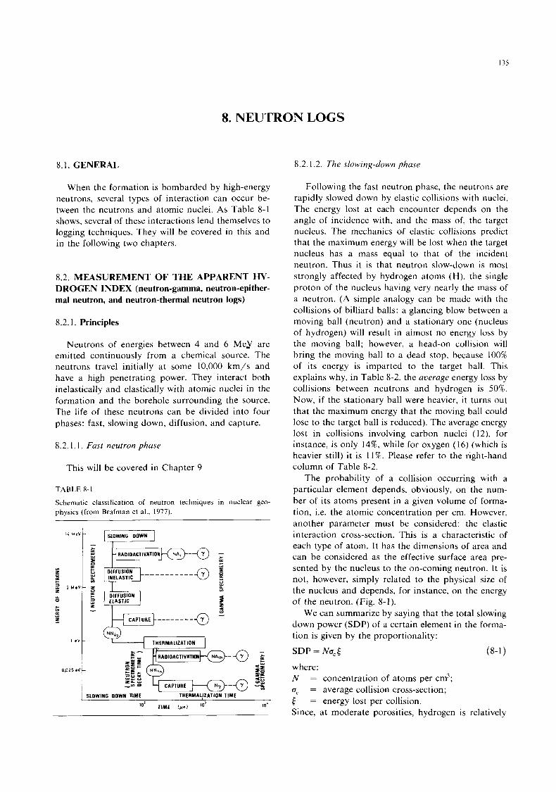
8. NEUTRON LOGS
8.1. GENERAL 8.2.1.2. The slowing-down phuse
When the formation is bombarded by high-energy neutrons, several types of interaction can occur be- tween the neutrons and atomic nuclei. As Table 8-1 shows, several of these interactions lend themselves to logging techniques. They will be covered in this and in the following two chapters.
8.2. MEASUREMENT OF THE APPARENT HY- DROGEN INDEX (neutron-gamma, neutron-epither- ma1 neutron, and neutron-thermal neutron logs)
8.2.1. Principles
Neutrons of energies between 4 and 6 MeY are emitted continuously from a chemical source. The neutrons travel initially at some 10,000 km/s and have a high penetrating power. They interact both inelastically and elastically with atomic nuclei in the formation and the borehole surrounding the source. The life of these neutrons can be divided into four phases: fast, slowing down, diffusion, and capture.
8.2.1.1. Fust neutron phuse
This will be covered in Chapter 9
TABLE 8-1
Schematic classification of neutron techniques in nuclear geo- physics (from Brafman et al., 1977).
Y
c
I e v t
I SLOWING I
loL
Following the fast neutron phase, the neutrons are rapidly slowed down by elastic collisions with nuclei. The energy lost at each encounter depends on the angle of incidence with, and the mass of, the target nucleus. The mechanics of elastic collisions predict that the maximum energy will be lost when the target nucleus has a mass equal to that of the incident neutron. Thus it is that neutron slow-down is most strongly affected by hydrogen atoms (H), the single proton of the nucleus having very nearly the mass of a neutron. (A simple analogy can be made with the collisions of billiard balls: a glancing blow between a moving ball (neutron) and a stationary one (nucleus of hydrogen) will result in aimost no energy loss by the moving ball; however, a head-on collision will bring the moving ball to a dead stop, because 100% of its energy is imparted to the target ball. This explains why, in Table 8-2, the uueruge energy loss by collisions between neutrons and hydrogen is 50%. Now, if the stationary ball were heavier, it turns out that the maximum energy that the moving ball could lose to the target ball is reduced). The average energy lost in collisions involving carbon nuclei (12). for instance, is only 14%, while for oxygen (16) (which is heavier still) it is 1 1 % . Please refer to the right-hand column of Table 8-2.
The probability of a collision occurring with a particular element depends, obviously, on the num- ber of its atoms present in a given volume of forma- tion, i.e. the atomic concentration per cm. However, another parameter must be considered: the elastic interaction cross-section. This is a characteristic of each type of atom. It has the dimensions of area and can be considered as the effective surface area pre- sented by the nucleus to the on-coming neutron. I t is not, however, simply related to the physical size of the nucleus and depends, for instance, on the energy of the neutron. (Fig. 8-1).
We can summarize by saying that the total slowing down power (SDP) of a certain element in the forma- tion is given by the proportionality:
SDP = Nu,( (8-1)
where: N a, = average collision cross-section; 5 = energy lost per collision. Since, at moderate porosities, hydrogen is relatively
= concentration of atoms per cm3;
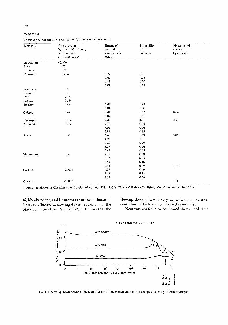
136
TABLE 8-2
Thermal neutron capture cross-section for the principal elements
Elements Cross-section in Energy of Probability Mean loss of barns ( = cm2) emitted of energy for neutrons gamma rays emission by collision ( u = 2200 m/s) (MeV)
Gadolinium 40,000 Bore 77 1 Lithium 71 Chlorine 33.4
Potassi um Barium Iron Sodium Sulphur
C a 1 c i u m
Hydrogen Aluminium
Silicon
Magnesium
2.2 1.2 2.56 0.534 0.49
0.44
0.332 0.232
0.16
0.064
7.77 7.42 6.12 5.01
0.1 0.08 0.06 0.04
5.43 0.84 4.84 0.20 6.42 0.83 5.89 0.11 2.23 1 .o 1.12 0.35 3.02 0.16 2.84 0.13 6.40 0.19 4.95 1 .0 4.20 0.19 3.57 0.94 2.69 0.65 8.16 0.09 3.92 0.83 3.45 0.16 3.83 0.39
Carbon 0.0034 4.95 0.49 4.05 0.15 3.05 0.36
Oxygen 0.0002 0.1 I
* From Handbook of Chemistry and Physics, 62 edition (1981-1982). Chemical Rubber Publishing Co., Cleveland, Ohio, U.S.A.
0.04
0.5
0.06
0.14
highly abundant, and its atoms are at least a factor of 10 more effective at slowing down neutrons than the other common elements (Fig. 8-2), i t follows that the
slowing down phase is very dependent on the con- centration of hydrogen or the hydrogen index.
Neutrons continue to be slowed down until their
CLEAN SAND, POROSITY 1 5 %
l 1
10-4 I I .1 1 10 1 0 2 1 0 3 1 0 4 1 6 10s 107
NEUTRON ENERGY I N ELECTRON VOLTS b s
d P idj f
Fig. 8-1. Slowing down power of H, 0 and Si for different incident neutron energies (courtesy of Schlumberger).
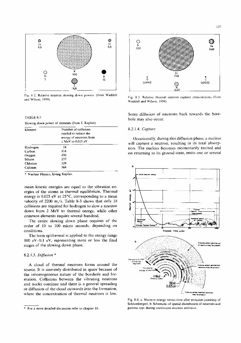
137
8 0
4.9 5,5 C I C a
0 t i 100 0
SI 0 7.
'*' I 1qa I
Fig. 8-2 . Relative neutron slowing down powers. (from Waddell and Wilson, 1959).
TABLE 8-3
Slowing down power of elements (from I. Kaplan)
Element Number of collisions needed to reduce the energy of neutrons from 2 MeV to 0.025 eV
Hydrogen 18 Carbon 1 I4 Oxygen 150 Silicon 251 Chlorine 329 Calcium 368
* Nuclear Physics, Irving Kaplan.
mean kinetic energies are equal to the vibration en- ergies of the atoms in thermal equilibrium. Thermal energy is 0.025 eV at 25"C, corresponding to a mean velocity of 2200 m/s. Table 8-3 shows that only 18 collisions are required for hydrogen to slow a neutron down from 2 MeV to thermal energy, whle other common elements require several hundred.
The entire slowing down phase requires of the order of 10 to 100 micro seconds, depending on conditions.
The term epithermal is applied to the energy range 100 eV-0.1 eV, representing more or less the final stages of the slowing down phase.
8.2.1.3. Diffusion *
A cloud of thermal neutrons forms around the source. It is unevenly distributed in space because of the inhomogeneous nature of the borehole and for- mation. Collisions between the vibrating neutrons and nuclei continue and there is a general spreading or diffusion of the cloud outwards into the formation, where the concentration of thermal neutrons is low.
* For a more detailed discussion refer to chapter 10.
0 SI CI
0.43 O J 3
C I 31.6 e
0 C OD032 @ 0,0002
Fig. 8-3. Relative thermal neutron capture cross-sections (from Waddell and Wilson, 1959).
Some diffusion of neutrons back towards the bore- hole may also occur.
8.2.1.4. Capture
Occasionally, during this diffusion phase, a nucleus will capture a neutron, resulting in its total absorp- tion. The nucleus becomes momentarily excited and on returning to its ground-state, emits one or several
a I I I
i
Elapsed time. psec
-v bo p-nt
Fig. 8-4. a. Neutron energy versus time after emission (courtesy of Schlumberger). b. Schematic of spatial distribution of neutrons and gamma rays during continuous neutron emission.
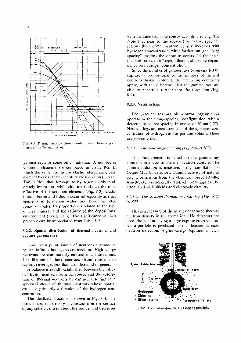
13x
0 5 10 15 20 25 30 35 40 45 50 55 60 65 7Qsentlrnstrrl
DISTANCE FROM SOURCE
Fig. X-5. Thermal neutron density with distance from a point source (from Tittman. 1956).
gamma rays, or some other radiation. A number of common elements are compared in Table 8-2. In much the same way as for elastic interactions, each element has its thermal capture cross-section (c in the Table). Note that, for capture, hydrogen is only mod- erately important, while chlorine ranks as the most effective of the common elements (Fig. 8-3). Gado- linium, boron and lithium occur infrequently as trace elements in formation water, and boron is often found in shales. Its proportion is related to the type of clay mineral and the salinity of the depositional environment (Fertl, 1973). The significance of their presence can be appreciated from Table 8-2.
8.2.2. Spatial distribution of thermal neutrons and capture gamma rays
Consider a point source of neutrons surrounded by an infinite homogeneous medium. High-energy neutrons are continuously emitted in all directions. The lifetime of these neutrons (from emission to capture) averages less than a millisecond in general.
A balance is rapidly established between the influx of “fresh” neutrons from the source and the absorp- tion of thermal neutrons by capture, resulting in a spherical cloud of thermal neutrons whose spatial extent is primarily a function of the hydrogen con- centration.
The idealized situation is shown in Fig. 8-4. The thermal neutron density is constant over the surface of any sphere centred about the source, and decreases
with distance from the source according to Fig. 8-5. Note that near to the source (the “short spacing’’ region) the thermal neutron density increases with hydrogen concentration, while farther out (the “long spacing” region) the opposite occurs. In the inter- mediate “cross-over’’ region there is almost no depen- dence on hydrogen concentration.
Since the number of gamma rays being emitted by capture is proportional to the number of thermal neutrons being captured, the preceding comments apply, with the difference that the gamma rays are able to penetrate further into the formation (Fig. 8-4).
8.2.3. Neutron logs
For practical reasons, all neutron logging tools operate in the ‘‘ long-spacing” configuration, with a detector to source spacing in excess of 30 cm (12”). Neutron logs are measurements of the apparent con- centration of hydrogen atoms per unit volume. There are several types.
8.2.3.1. The neutron-gamma log (Fig. 8-6) (GNT)
This measurement is based on the gamma ray emission rate due to thermal neutron capture. The gamma radiation is measured using scintillation or Geiger-Mueller detectors. Gamma activity of natural origin, or arising from the chemical source (Ra-Be, Am-Be, etc.,) is generally relatively weak and can be attenuated with shields and electronic circuitry.
8.2.3.2. The neutron-thermal neutron log (Fig. 8-7)
(CNT)
This is a measure of the as yet uncaptured thermal neutron density in the formation. ‘He detectors are used, the helium having a large capture cross-section. An a-particle is produced in the detector at each neutron detection. Higher energy (epithermal, etc.)
Fig. 8-6. The neutron-gamma (n,y) logging principle.
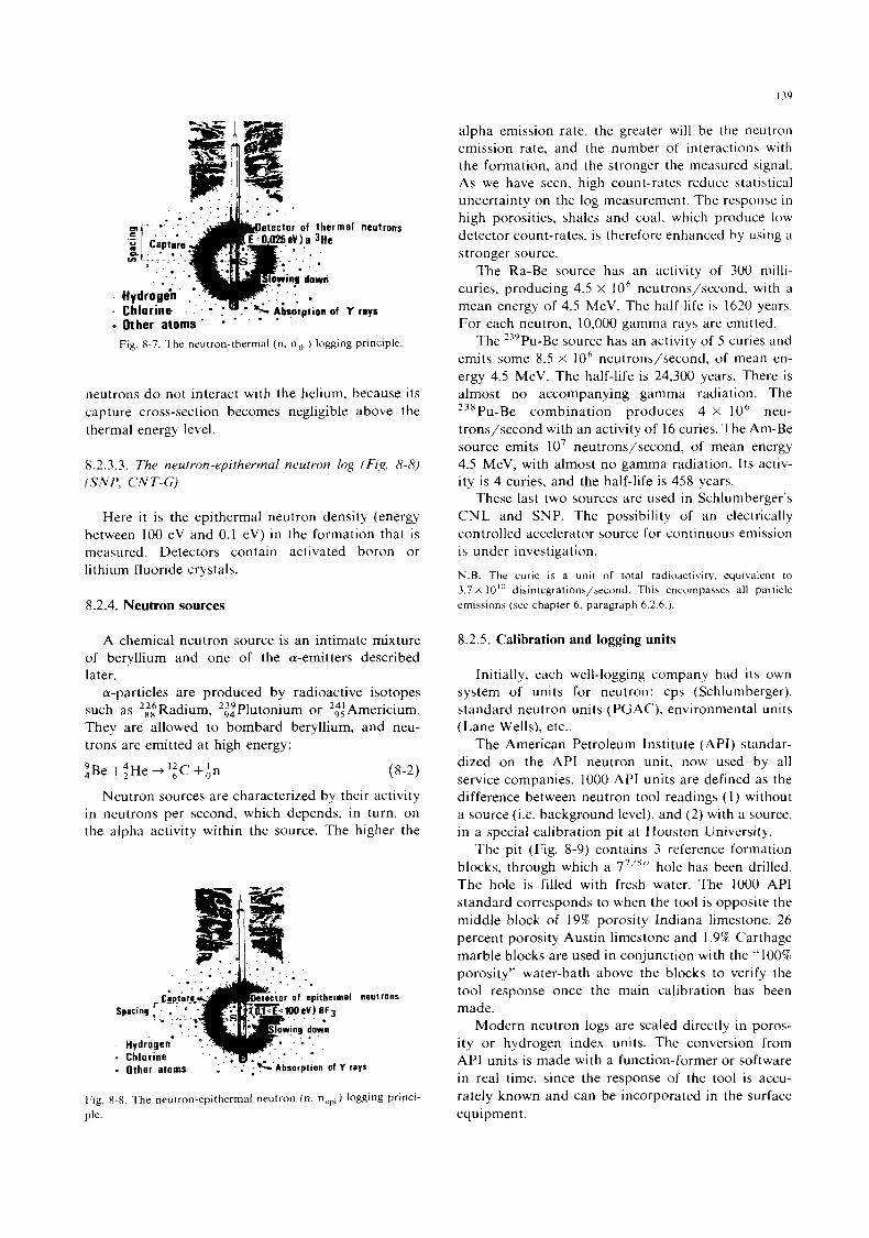
0 Other atoms‘ ’ - . ’ ’ ‘ ’ ‘
Fig. 8-7. The neutron-thermal (n. nlh ) logging principle.
neutrons d o not interact with the helium, because its capture cross-section becomes negligible above the thermal energy level.
8.2.3.3. The neutron-epithermal neutron log (Fig. 8-8) ( S N P , CNT-G)
Here it is the epithermal neutron density (energy between 100 eV and 0.1 eV) in the formation that is measured. Detectors contain activated boron or lithium fluoride crystals.
8.2.4. Neutron sources
A chemical neutron source is an intimate mixture of beryllium and one of the a-emitters described later.
a-particles are produced by radioactive isotopes such as *::Radium, *::Plutonium or ’;:Americium. They are allowed to bombard beryllium, and neu- trons are emitted at high energy:
~ B e + ~ H e - + l ~ C + ~ n (8-2) Neutron sources are characterized by their activity
in neutrons per second, which depends, in turn, on the alpha activity within the source. The higher the
Fig. 8-8. The neutron-epithermal neutron (n, ncp, ) logging princi- ple.
alpha emission rate, the greater will be the neutron emission rate. and the number of interactions with the formation, and the stronger the measured signal. As we have seen, high count-rates reduce statistical uncertainty on the log measurement. The response i n high porosities, shales and coal, which produce low detector count-rates, is therefore enhanced by using a stronger source.
The Ra-Be source has an activity of 300 niilli- curies, producing 4.5 x lo6 neutrons/second, with a mean energy of 4.5 MeV. The half-life is 1620 years. For each neutron, 10,000 gamma rays are emitted.
The ”’Pu-Be source has an activity o f 5 curies and emits some 8.5 X 10‘ neutrons/second. of mean en- ergy 4.5 MeV. The half-life is 24,300 years. There is almost no accompanying gamma radiation. The 238Pu-Be combination produces 4 X 10‘ neu- trons/second with an activity of 16 curies. The Am-Be source emits lo7 neutrons/second, of mean energy 4.5 MeV, with almost no gamma radiation. Its activ- ity is 4 curies, and the half-life is 458 years.
These last two sources are used in Schlumberger’s CNL and SNP. The possibility of an electrically controlled accelerator source for continuous emission is under investigation. N.B. The curie is a unit of total radioactivity, equivalent to 3.7 X 10“’ disintegrations/second. This encompaases all particle emissions (see chapter 6. paragraph 6.2.6.).
8.2.5. Calibration and logging units
Initially, each well-logging company had its own system of units for neutron: cps (Schlumberger), standard neutron units (PGAC), environmental units (Lane Wells), etc..
The American Petroleum Institute (API) standar- dized on the API neutron unit, now used by all service companies. 1000 API units are defined as the difference between neutron tool readings ( I ) without a source (i.e. background level), and (2) with a source, in a special calibration pit at Houston University.
The pit (Fig. 8-9) contains 3 reference formation blocks, through which a 7’IX” hole has been drilled. The hole is filled with fresh water. The 1000 API standard corresponds to when the tool is opposite the middle block of 19% porosity Indiana limestone. 26 percent porosity Austin limestone and 1.9% Carthage marble blocks are used in conjunction with the “100% porosity” water-bath above the blocks to verify the tool response once the main calibration has been made.
Modern neutron logs are scaled directly in poros- i ty or hydrogen index units. The conversion from API units is made with a function-former or software in real time, since the response of the tool is accu- rately known and can be incorporated in the surface equipment.
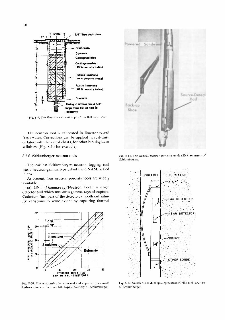
I40
(1.9 % porosity index)
Indiana linwrtone (19 % porosity index)
Austin limestone (26 96 porosity index)
b i n g in r.tholo ha id 1/8"
Fig. X-9. The Houston calibration pit (from Belknap. 1959).
The neutron tool is calibrated in limestones and fresh water. Corrections can be applied in real-time, or later, with the aid of charts, for other lithologies or salinities. (Fig. 8-10 for example).
8.2.6. Schlumberger neutron tools
The earliest Schlumberger neutron logging tool was a neutron-gamma type called the GNAM, scaled in cps.
At present, four neutron porosity tools are widely available.
(a) GNT (Gamma-ray/Neutron Tool): a single detector tool which measures gamma-rays of capture. Cadmium fins, part of the detector, smooth out salin- i ty variations to some extent by capturing thermal
HYDROGEN INOEX FOR SNP and CNL ( LIMESTONE I
I..ig. X-10. The relationship between real and apparent (measured) hydrogen indices for three lithologies (courtesy o f Schlumberger).
tector
Fig. 8-1 I. The sidewall neutron porosity sonde (SNP) (courtesy of Schlumberger)
. . . . . .
. -. ' . . BOREHOLE
. . . . . . . . . . . . . . . . . . . . . . : . . . . . .
. . . . . . . .
. . . . . . . . . _ . . . . . . . .
Y
. . . . . . . . . . . . . . . . . . . . .
. . . . ':' FORMAT(0N.: : . . . . . . . . . . . . . .
/ - 3 3/8' .DlA. . . . . . . . . . . . .
. . . . . . . . .
. . . . . . _ _ . _ . - . . . . . . . . . . . . . . . . . . , . . . _ .
. . . . . . . _ _ _ &F.AR . . ' :DETECTOR.. . . . . .
. . . . . . . . . . . . . . . .
. . . . . . . . . . . . . . . .
. . . . . . _ , _ . . . .
-NEAR DETECTOR, . . . . . . . . . . . . .
. - . ,
: . . . . . . . . . . . . . .
. . :_ - . .
. . .
. . . . . .
. . , . . I . . . . . .
-SOURCE
. . . . . . . . . ' . . . . . . . . . . . . . .
>OTHER SONDE : . . . . . . . . . . . . . . . . . . .
. . . . . . . . . . . . . . . . .
. . . . . . . . . . . . . . . . . .
. . . . .
. . . . . . . . . . . . . . . . . . . .
. . _ .
Fig 8-12. Sketch of the dual-\pacing neutron (CNL) tool (courtesy of Schlumberger)
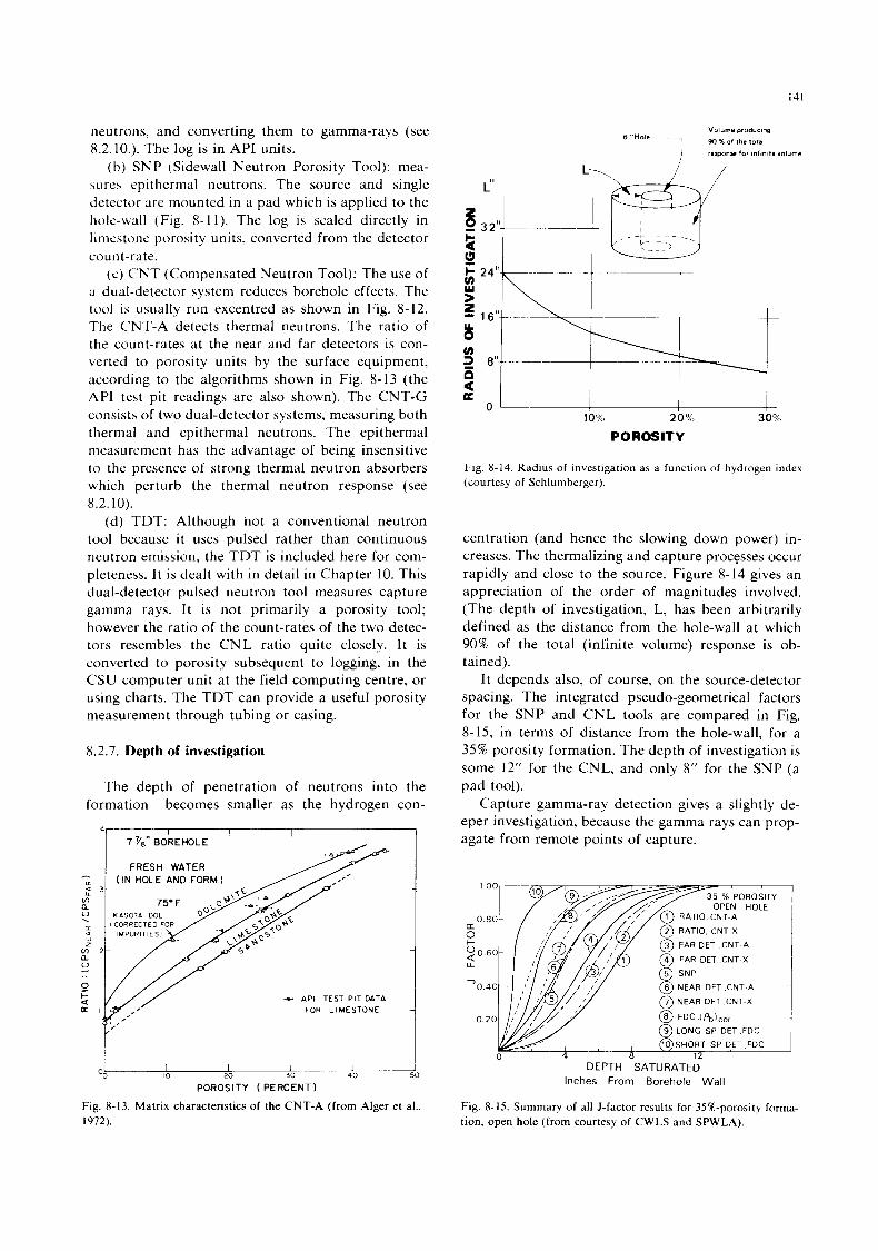
141
neutrons, and converting them to gamma-rays (see 8.2.10.). The log is in API units.
( b ) SNP (Sidewall Neutron Porosity Tool): mea- sures epithermal neutrons. The source and single detector are mounted in a pad which is applied to the hole-wall (Fig. 8-1 I ) . The log is scaled directly in limestone porosity units, converted from the detector count-rate.
(c) CNT (Compensated Neutron Tool): The use of ;1 dual-detector system reduces borehole effects. The tool is usually run excentred as shown in Fig. 8-12. The CNT-A detects thermal neutrons. The ratio of the count-rates at the near and far detectors is con- verted to porosity units by the surface equipment, according to the algorithms shown in Fig. 8-13 (the API test pit readings are also shown). The CNT-G consists of two dual-detector systems, measuring both thermal and epithermal neutrons. The epithermal measurement has the advantage of being insensitive to the presence of strong thermal neutron absorbers which perturb the thermal neutron response (see 8.2.10).
(d) TDT: Although not a conventional neutron tool because i t uses pulsed rather than continuous neutron emission, the TDT is included here for com- pleteness. I t is dealt with in detail in Chapter 10. This dual-detector pulsed neutron tool measures capture gamma rays. I t is not primarily a porosity tool; however the ratio of the count-rates of the two detec- tors resembles the CNL ratio quite closely. I t is converted to porosity subsequent to logging, in the CSU computer unit at the field computing centre, or using charts. The TDT can provide a useful porosity measurement through tubing or casing.
8.2.7. Depth of investigation
The depth of penetration of neutrons into the formation becomes smaller as the hydrogen con-
7 '/a'' BOREHOLE ' FRESH WATER
I I
a
+ API TEST PIT DATA FOR LIMESTONE
00 - 20 30
POROSITY ( PERCENT)
Fig. 8-13, Matrix characteristics of the CNT-A (from Alger et al., 1972).
Volurna producing
90 4 of Ihe total 6 Hole
re,ponIm for lnllnlle YolUme
L\ L"
I I
10% 2 0 % 30%
POROSITY
Fig. 8-14. Radius of investigation as a function of hydrogen index (courtesy of Schlumberger).
centration (and hence the slowing down power) in- creases. The thermalizing and capture processes occur rapidly and close to the source. Figure 8-14 gives an appreciation of the order of magnitudes involved. (The depth of investigation, L, has been arbitrarily defined as the distance from the hole-wall at which 90% of the total (infinite volume) response is ob- tained).
It depends also, of course, on the source-detector spacing. The integrated pseudo-geometrical factors for the SNP and CNL tools are compared in Fig. 8-15, in terms of distance from the hole-wall, for a 35% porosity formation. The depth of investigation is some 12" for the CNL, and only 8" for the SNP (a pad tool).
Capture gamma-ray detection gives a slightly de- eper investigation, because the gamma rays can prop- agate from remote points of capture.
AT10 CNT A
AT10 CNT X
FAR DET CNT A
FAR DET CNT X
NEAR DET CNT A
NEAR DET CNT X
LONG SP DET FDC
DEPTH SATURATED Inches From Borehole Wall
Fig. 8-15. Summary of all J-factor results for 35%-porosity forma- tion, open hole (from courtesy of CWLS and SPWLA).
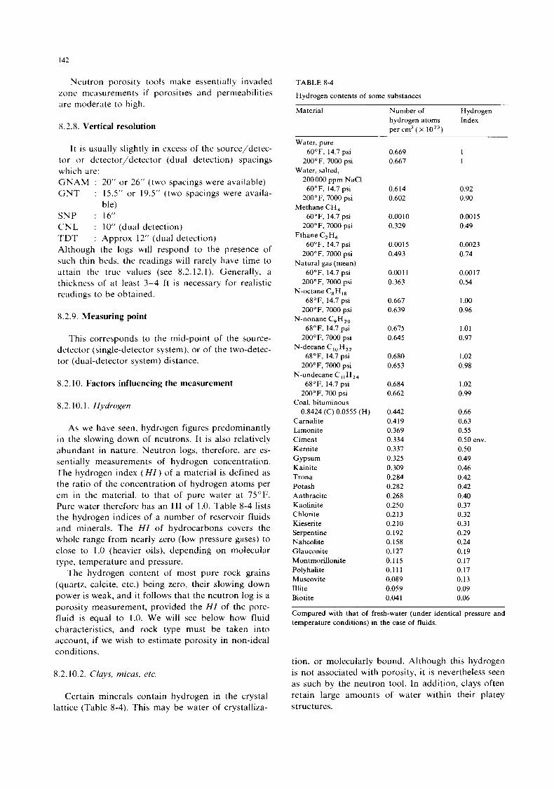
I42
Neutron porosity tools make essentially invaded zone measurements i f porosities and permeabilities are moderate to high.
8.2.8. Vertical resolution
I t is usually slightly in excess of the source/detec- tor o r detector/detector (dual detection) spacings which are: GNAM : 20" o r 26" (two spacings were available) G N T : 15.5" or 19.5" (two spacings were availa-
ble) SNP : 16" CNL : 10" (dual detection) TDT Although the logs will respond to the presence of xuch thin beds, the readings will rarely have time to attain the true values (see 8.2.12.1). Generally. a thickness of at least 3-4 f t is necessary for realistic readings to be obtained.
: Approx 12" (dual detection)
8.2.9. Measuring point
This corresponds to the mid-point of the source- detector (single-detector system), or of the two-detec- tor (dual-detector system) distance.
8.2.10. Factors influencing the measurement
8.2.10.1. H.ydrogen
As we have seen. hydrogen figures predominantly in the slowing down of neutrons. I t is also relatively abundant in nature. Neutron logs, therefore, are es- sentially measurements of hydrogen concentration. The hydrogen index ( H I ) of a material is defined as the ratio of the concentration of hydrogen atoms per cm in the material, to that of pure water at 75°F. Pure water therefore has an HI of 1.0. Table 8-4 lists the hydrogen indices of a number of reservoir fluids and minerals. The HZ of hydrocarbons covers the whole range from nearly zero (low pressure gases) to close to 1.0 (heavier oils), depending on molecular type, temperature and pressure.
The hydrogen content of most pure rock grains (quartz, calcite, etc.) being zero, their slowing down power is weak, and i t follows that the neutron log is a porosity measurement, provided the H I of the pore- fluid is equal to 1.0. We will see below how fluid characteristics, and rock type must be taken into account, i f we wish to estimate porosity in non-ideal conditions.
8.2.10.2. Clays, micas, etc.
Certain minerals contain hydrogen in the crystal lattice (Table 8-4). This may be water of crystalliza-
TABLE 8-4
Hydrogen contents of some substances
Material Number of Hydrogen hydrogen atoms Index per cm3 ( x 1 0 , ~ )
Water, pure 60°F, 14.7 psi
200"F, 7000 psi
200000 ppm NaCl 60°F. 14.7 psi
200"F, 7000 psi
60°F, 14.7 psi 200"F, 7000 psi
60°F, 14.7 psi 200°F, 7000 psi
Natural gas (mean) 60°F, 14.7 psi
200°F. 7000 psi
68"F, 14.7 psi 200'F. 7000 psi
N-nonane C,H,,, 68"F, 14.7 psi
200" F, 7000 psi N-decane C,,H,,
68'F. 14.7 psi 200'F, 7000 psi
N-undecane C I I H,, 68°F. 14.7 psi
200"F, 700 psi Coal, bituminous
0.8424 (C) 0.0555 (H) Carnalite Limonite Ciment Kernite Gypsum Kainite Trona Potash Anthracite Kaolinite Chlorite Kieserite Serpentine Nahcolite Glauconite Montmorillonite Polyhalite Muscovite Illite Biotite
Water, salted,
Methane CH,
Ethane C,H,
N-octane C, H
0.669 0.667
0.614 0.602
0.0010 0.329
0.00 15 0.493
0.001 1 0.363
0.667 0.639
0.675 0.645
0.680 0.653
0.684 0.662
0.442 0.4 19 0.369 0.334 0.337 0.325 0.309 0.284 0.282 0.268 0.250 0.213 0.210 0.192 0.158 0.127 0.115 0.1 1 1 0.089 0.059 0.041
1 1
0.92 0.90
0.00 15 0.49
0.0023 0.74
0.0017 0.54
1 .oo 0.96
1.01 0.97
1.02 0.98
1.02 0.99
0.66 0.63 0.55 0.50 env. 0.50 0.49 0.46 0.42 0.42 0.40 0.37 0.32 0.31 0.29 0.24 0.19 0.17 0.17 0.13 0.09 0.06
Compared with that of fresh-water (under identical pressure and temperature conditions) in the case of fluids.
tion, or molecularly bound. Although this hydrogen is not associated with porosity, it is nevertheless seen as such by the neutron tool. In addition, clays often retain large amounts of water within their platey structures.
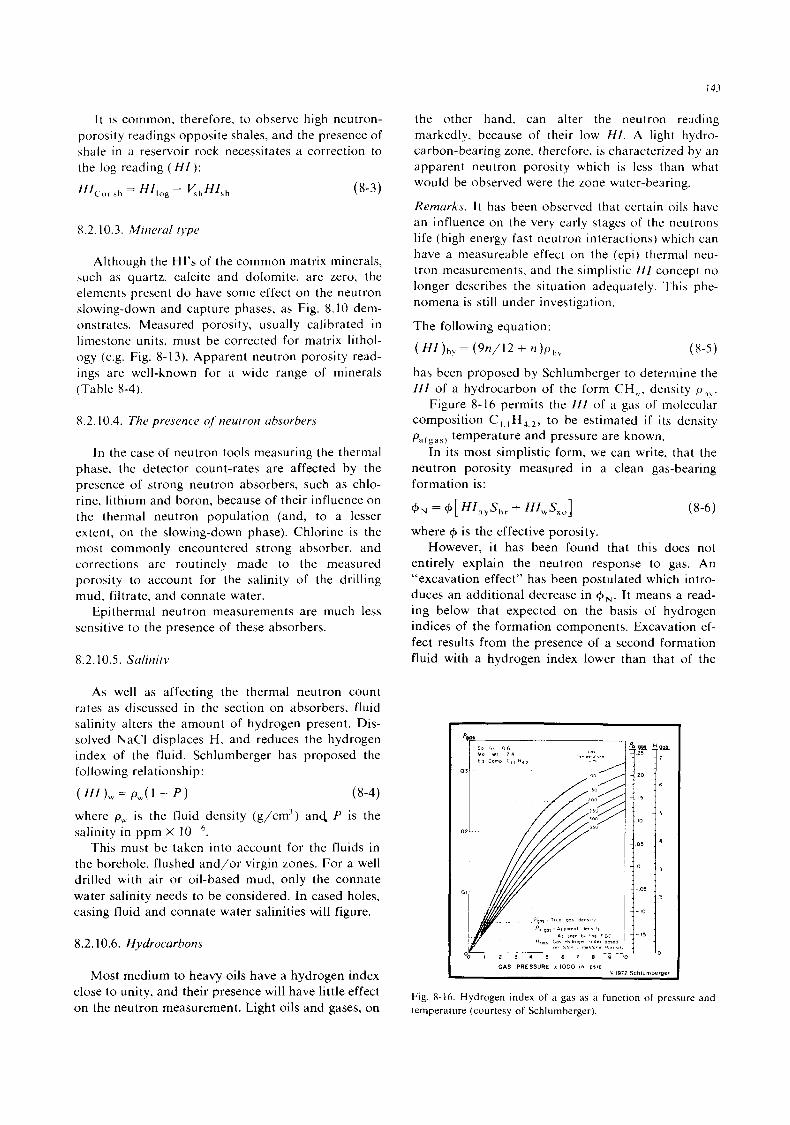
143
I t is common, therefore, to observe high neutron- porosity readings opposite shales, and the presence of shale i n a reservoir rock necessitates a correction to the log reading ( H I ):
HICor ,h = H 1 , o g - yhH’sh (8-3)
8.2.10.3. Mineral type
Although the HI’S of the common matrix minerals, such as quartz, calcite and dolomite, are zero, the elements present do have some effect on the neutron slowing-down and capture phases, as Fig. 8.10 dem- onstrates Measured porosity, usually calibrated in limestone units, must be corrected for matrix lithol- ogy (e.g. Fig. 8-13). Apparent neutron porosity read- ings are well-known for a wide range of minerals (Table 8-4).
8.2.10.4. The presence of neutron absorbers
I n the case of neutron tools measuring the thermal phase, the detector count-rates are affected by the presence of strong neutron absorbers, such as chlo- rine, lithium and boron, because of their influence on the thermal neutron population (and, to a lesser extent, on the slowing-down phase). Chlorine is the most commonly encountered strong absorber, and corrections are routinely made to the measured porosity to account for the salinity of the drilling mud, filtrate, and connate water.
Epithermal neutron measurements are much less sensitive t o the presence of these absorbers.
8.2.10.5. Salinitv
As well as affecting the thermal neutron count rates as discussed in the section on absorbers, fluid salinity alters the amount of hydrogen present. Dis- solved NaCl displaces H, and reduces the hydrogen index of the fluid. Schlumberger has proposed the following relationship:
( H I ) w = p , ( l - p ) (8-4)
where p, is the fluid density (g/cm7) and P is the salinity in ppm x lo-‘.
This must be taken into account for the fluids in the borehole, flushed and/or virgin zones. For a well drilled with air or oil-based mud, only the connate water salinity needs to be considered. In cased holes, casing fluid and connate water salinities will figure.
8.2.10.6. Hydrocarbons
Most medium to heavy oils have a hydrogen index close to unity, and their presence will have little effect on the neutron measurement. Light oils and gases, on
the other hand, can alter the neutron reading markedly, because of their low H I . A light hydro- carbon-bearing zone, therefore, is characterized by an apparent neutron porosity which is less than what would be observed were the zone water-bearing.
Remarks. I t has been observed that certain oils have an influence on the very early stages of the neutrons life (high energy fast neutron interactions) which can have a measureable effect on the (epi) thermal neu- tron measurements, and the simplistic H I concept no longer describes the situation adequately. This phe- nomena is still under investigation.
The following equation:
( H I ) h , = (9fl/12 + f l ) P h y ( 8 - 5 )
has been proposed by Schlumberger to determine the H I of a hydrocarbon of the form CH,,, density p,,,.
Figure 8-16 permits the H I of a gas of molecular composition C, , ,H,2, to be estimated if its density pa(gas) temperature and pressure are known.
In its most simplistic form, we can write, that the neutron porosity measured in a clean gas-bearing formation is:
@ N = @[ H’hyShr + H1wSxO] (8-6)
where is the effective porosity. However, it has been found that this does not
entirely explain the neutron response to gas. An “excavation effect” has been postulated which intro- duces an additional decrease in G N . It means a read- ing below that expected on the basis of hydrogen indices of the formation components. Excavation ef- fect results from the presence of a second formation fluid with a hydrogen index lower than that of the
Fig. 8-16. Hydrogen index of a gas as a function of pressure and temperature (courtesy of Schlumberger).
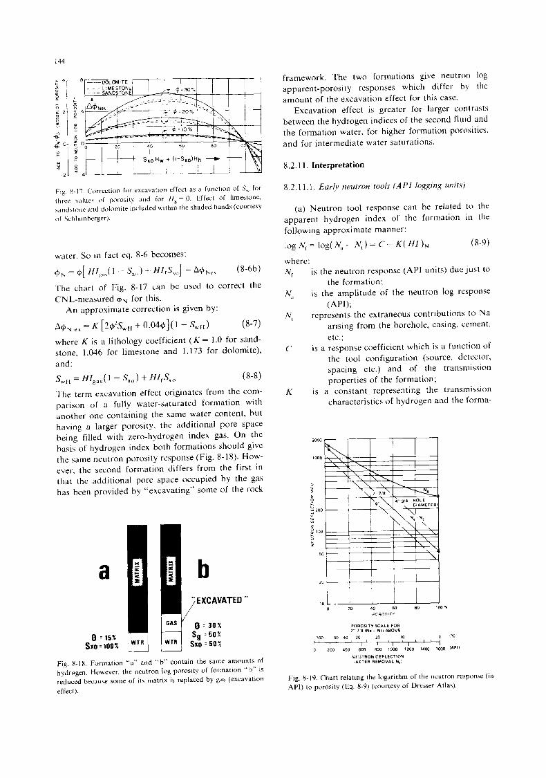
144
Fig. X-17. Correction for excavation effect as a function of S, for three viilues c ) f porosity and for H , = 0. Effect of limestone. \nndstone and dolomite included within the shaded bands (courtesy of Schlumberger).
water. So in fact eq. 8-6 becomes:
+ N = $[ H 1 g ~ t , ( ’ ~ sx,,) + H z , S x O ] - A + N c , (8-6b)
The chart of Fig. 8-17 can be used to correct the CNL-measured + N for this.
An approximate correction is given by:
A$N e x = K [2+2SwH + O.O4+](1 - Sw,) (8-7) where K is a lithology coefficient ( K = 1 .O for sand- stone, 1.046 for limestone and 1.173 for dolomite), and:
Sw,, = f f & J I - SX,> + HIfSx, (8-8) The term excavation effect originates from the com- parison of a fully water-saturated formation with another one containing the same water content, but having a larger porosity, the additional pore space being filled with zero-hydrogen index gas. On the basis of hydrogen index both formations should give the same neutron porosity response (Fig. 8-18). How- ever, the second formation differs from the first in that the additional pore space occupied by the gas has been provided by “excavating” some of the rock
a
8 = 15% sxo = 100 %
Fig. 8-18. Formation “a” and “b” contain the same amounts of hydrogen. However, the neutron log porosity of formation “b” is reduced because some of its matrix is replaced by gas (excavation effect).
framework. The two formations give neutron log apparent-porosity responses which differ by the amount of the excavation effect for this case.
Excavation effect is greater for larger contrasts between the hydrogen indices of the second fluid and the formation water, for higher formation porosities. and for intermediate water saturations.
8.2.1 1. Interpretation
8.2.1 1.1. E a r b neutron tools (API logging units)
(a) Neutron tool response can be related to the apparent hydrogen index of the formation in the following approximate manner:
log N f = log( N, - N , ) = C - K ( H I ) N (8-9) where:
is the neutron response (API units) due just to the formation;
is the amplitude of the neutron log response (API);
represents the extraneous contributions to Na arising from the borehole, casing, cement. etc.;
is a response coefficient which is a function of the tool configuration (source. detector, spacing etc.) and of the transmission properties of the formation;
is a constant representing the transmission characteristics of hydrogen and the forma-
2000 t 1
1000
~
3 P u u 200
50
1 1 t I I I
20 -1 10
0 20 40 60 80 100 3
POROSITY
POROSITY SCALE FOR 7 ’ 7 8 IN. ~ Nil ABOVE
1 1 1 I , 1W 50 40 30 20 10 0 ipb l
& I
0 200 400 6W 800 1OW 1200 14W 1600 IAPII I I I ” I I 1 I , ,
NEUTRON DEFLECTION (AFTER REMOVAL Ntl
Fig. 8-19. Chart relating the logarithm of the neutron response (in API) to porosity (Eq. 8-9) (courtesy of Dresser Atlas).
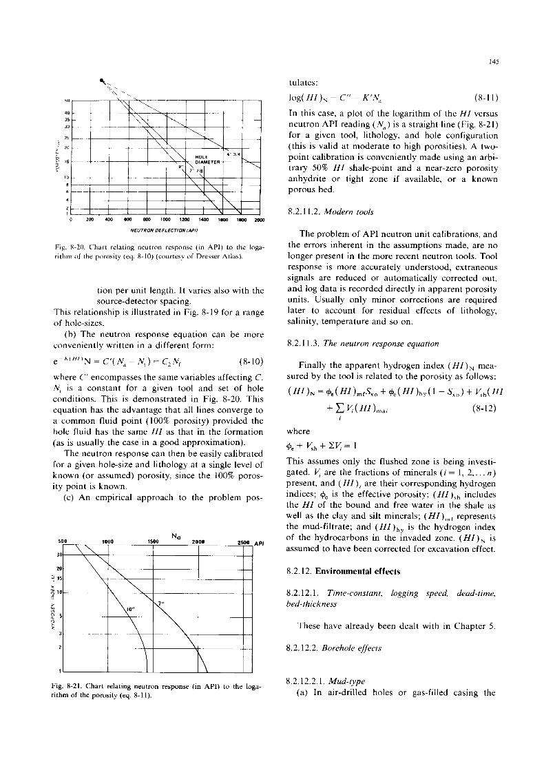
14.5
0 zw 4MI 800 800 loo0 lmo l4m 1m 1m moo
NEUTRON DEFLECTION *PI /
Fig. X-20. Chart relating neutron response (in API) to the loga- rithm o f the porosity (eq. 8-10) (courtesy of Dresser Atlas).
tion per unit length. It varies also with the source-detector spacing.
This relationship is illustrated in Fig. 8-19 for a range of hole-sizes.
(b) The neutron response equation can be more conveniently written in a different form:
e-h('")N = C ! ( N 'I - N 1 ) = c 2 f N (8-10)
where C' encompasses the same variables affecting C. N , is a constant for a given tool and set of hole conditions. This is demonstrated in Fig. 8-20. This equation has the advantage that all lines converge to a common fluid point (100% porosity) provided the hole fluid has the same H I as that in the formation (as is usually the case in a good approximation).
The neutron response can then be easily calibrated for a given hole-size and lithology at a single level of known (or assumed) porosity, since the 100% poros- ity point is known.
(c) An empirical approach to the problem pos-
9PI
Fig. 8-21. Chart relating neutron response (in API) to the loga- rithm of the porosity (eq. 8-1 1).
tulates:
log( H I ) N = C" - K ' N , (8-1 1 )
In this case, a plot of the logarithm of the HI versus neutron API reading ( N , ) is a straight line (Fig. 8-21) for a given tool, lithology, and hole configuration (this is valid at moderate to high porosities). A two- point calibration is conveniently made using an arbi- trary 50% HI shale-point and a near-zero porosity anhydrite or tight zone if available, or a known porous bed.
8.2.1 1.2. Modern tools
The problem of API neutron unit calibrations, and the errors inherent in the assumptions made, are no longer present in the more recent neutron tools. Tool response is more accurately understood, extraneous signals are reduced or automatically corrected out, and log data is recorded directly in apparent porosity units. Usually only minor corrections are required later to account for residual effects of lithology, salinity, temperature and so on.
8.2.11.3. The neutron response equation
Finally the apparent hydrogen index ( H I ) , mea- sured by the tool is related to the porosity as follows:
( ) N = $e ( H I )rnfSxo + $e ( H I )h y ( - Sx,, + ?h (
+ c Y(HI)rna, (8-12) I
where G e + V,,+zy= 1
This assumes only the flushed zone is being investi- gated. y are the fractions of minerals ( i = 1, 2,. . . n ) present, and ( H I ) , are their corresponding hydrogen indices; $e is the effective porosity; ( H I ) s h includes the H I of the bound and free water in the shale as well as the clay and silt minerals; ( represents the mud-filtrate; and ( H I ) h T is the hydrogen index of the hydrocarbons in the invaded zone. ( H I ) , is assumed to have been corrected for excavation effect.
8.2.12. Environmental effects
8.2.12.1. Time-constant, logging speed, deud-time, bed-thickness
These have already been dealt with in Chapter 5.
8.2.12.2. Borehole effects
8.2.12.2.1. Mud-type (a) In air-drilled holes or gas-filled casing the
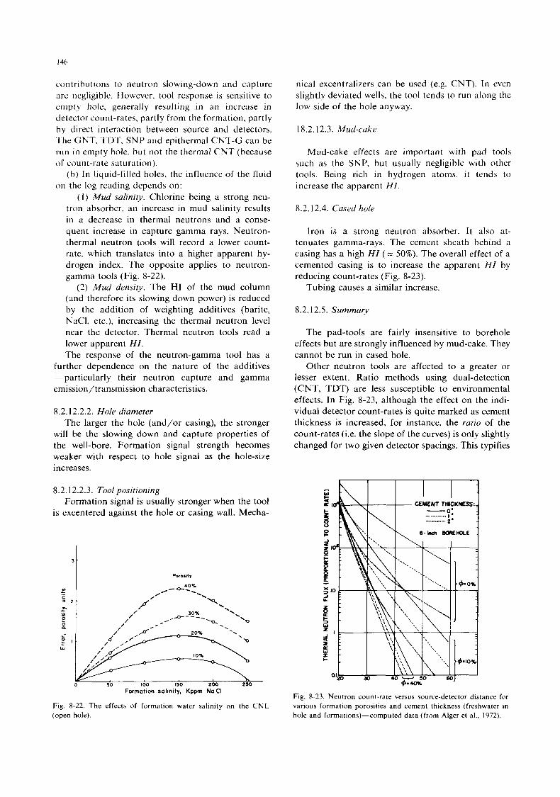
contributions to neutron slowing-down and capture are negligible. However. tool response is sensitive to empty hole, generally resulting in an increase in detector count-rates, partly from the formation, partly by direct interaction between source and detectors. The GNT. TDT. SNP and epithermal CNT-G can be r u n i n empty hole, but not the thermal CNT (because o f count-rate saturation).
(b) In liquid-filled holes, the influence of the fluid o n the log reading depends on:
( I ) Mud salinity. Chlorine being a strong neu- tron absorber, an increase in mud salinity results in a decrease in thermal neutrons and a conse- quent increase in capture gamma rays. Neutron- thermal neutron tools will record a lower count- rate, which translates into a higher apparent hy- drogen index. The opposite applies to neutron- gamma tools (Fig. 8-22).
(2) Mud density. The HI of the mud column (and therefore its slowing down power) is reduced by the addition of weighting additives (barite, NaCI, etc.), increasing the thermal neutron level near the detector. Thermal neutron tools read a lower apparent HI . The response of the neutron-gamma tool has a
further dependence on the nature of the additives -particularly their neutron capture and gamma emission/transmission characteristics.
8.2.12.2.2. Hole diameter The larger the hole (and/or casing), the stronger
will be the slowing down and capture properties of the well-bore. Formation signal strength becomes weaker with respect to hole signal as the hole-size increases.
8.2.12.2.3. Tool positioning Formation signal is usually stronger when the tool
is excentered against the hole or casing wall. Mecha-
M
c c .-
c
3 2 - 2,
0 so I S 0 2 0 0 2so
I/ ,’ ’
Formation salinity, Kppm Na CI
Fig. 8-22. The effects of formation water salinity on the CNL (open hole).
nical excentralizers can be used (e.g. CNT). I n even slightly deviated wells, the tool tends to run along the low side of the hole anyway.
18.2.12.3. Mud-cuke
Mud-cake effects are important with pad tools such as the SNP, but usually negligible with other tools. Being rich in hydrogen atoms, i t tends to increase the apparent H I .
8.2.12.4. Cased hole
Iron is a strong neutron absorber. I t also at- tenuates gamma-rays. The cement sheath behind a casing has a high HZ (= 50%). The overall effect of a cemented casing is to increase the apparent H I by reducing count-rates (Fig. 8-23).
Tubing causes a similar increase.
8.2.12.5. Summary
The pad-tools are fairly insensitive to borehole effects but are strongly influenced by mud-cake. They cannot be run in cased hole.
Other neutron tools are affected to a greater or lesser extent. Ratio methods using dual-detection (CNT, TDT) are less susceptible to environmental effects. In Fig. 8-23, although the effect on the indi- vidual detector count-rates is quite marked as cement thickness is increased, for instance, the ratio of the count-rates (i.e. the slope of the curves) is only slightly changed for two given detector spacings. T h s typifies
Fig. 8-23. Neutron count-rate versus source-detector distance for various formation porosities and cement thickness (freshwater in hole and formations)-computed data (from Alger et al.. 1972).
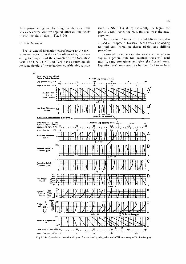
147
the improvement gained by using dual detectors. The necessary corrections are applied either automatically o r with the aid of charts (Fig. 8-24).
8.2.12.6. Inuasion
The volume of formation contributing to the mea- surement depends on the tool configuration, the mea- suring technique. and the character of the formation itself. The GNT, CNT and TDT have approximately the same depths of investigation, considerably greater
than the SNP (Fig. 8-15). Generally, the higher the porosity (and hence the H I ) , the shallower the niea- surement.
The process of invasion of mud filtrate was dis- cussed in Chapter 2. Invasion depth varies according to mud and formation characteristics and drilling procedure.
Taking all these factors into consideration. we can say as a general rule that neutron tools will read mostly, (and sometimes entirely), the flushed zone. Equation 8-12 may need to be modified to include
a Enter b e for lbqa withcut
Neutron Log Porosity Index pukmmtic cnllp CamCtKm
40 hap p ~ w to Jon. 1976 ? 10 20 30 l . , , , - ( . . . , . . l . . , . l , . , , . . , , " ' I " ' ' 7 ' 1
I . , . .
Lws after Jon. 1976 0 10 20 I 30 40
A'
Mud Coke Thichnrss- , B' Inchss
T
I A Mud ca* T h l C h U - Inches
A d z - I 0 ' / 0 t
B 25
Borehd. Salinity- Thouaond ppm
I l l l l l l l l l l l l l 1 . 1 1 1 1 1
I A d = + 0 4
Fomailm Salinlty- Thousand ppm
250
I, I I 1 Y l I I I
0 M I I I M I I I m
C
t
E
?"iI$ -6 F 0
sl6 t
G Borehole Tempcroture-
'F
Jo 1 . L u l
Loqs prior to Jon, I976 0 I) 20 30 I I I
Lops offer Jon , 1976 3 I0 x) 30 40
Fig 8-24a Open-hole correction diagram for the dual spacing (thermal) CNL (courtesy of Schlumberger)
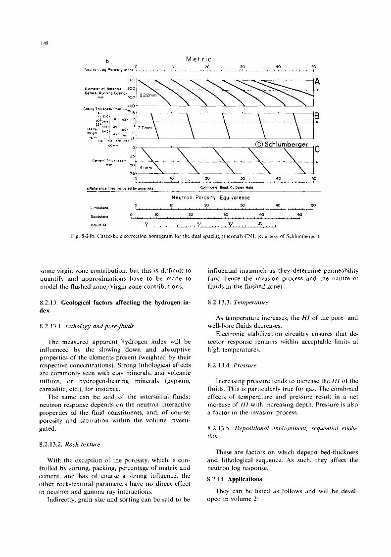
148
some virgin zone contribution, but this is difficult to quantify and approximations have to be made to model the flushed zone/virgin zone contributions.
8.2.13. Geological factors affecting the hydrogen in- dex
8.2.13.1. Lithology und pore-fluids
The measured apparent hydrogen index will be influenced by the slowing down and absorptive properties of the elements present (weighted by their respective concentrations). Strong lithological effects are commonly seen with clay minerals, and volcanic tuffites, or hydrogen-bearing minerals (gypsum, carnallite, etc.), for instance.
The same can be said of the interstitial fluids; neutron response depends on the neutron interactive properties of the fluid constituents, and, of course, porosity and saturation within the volume investi- gated.
8.2.13.2. Rock texture
With the exception of the porosity, which is con- trolled by sorting, packing, percentage of matrix and cement, and has of course a strong influence, the other rock-textural parameters have no direct effect in neutron and gamma ray interactions.
Indirectly, grain size and sorting can be said to be
influential inasmuch as they determine permeability (and hence the invasion process and the nature of fluids in the flushed zone).
8.2.1 3.3. Temperature
As temperature increases, the H I of the pore- and well-bore fluids decreases.
Electronic stabilization circuitry ensures that de- tector response remains within acceptable limits at high temperatures.
8.2.13.4. Pressure
Increasing pressure tends to increase the H I of the fluids. This is particularly true for gas. The combined effects of temperature and pressure result in a net increase of H I with increasing depth. Pressure is also a factor in the invasion process.
8.2.13.5. Depositional environment, sequentiul evolu- tion
These are factors on which depend bed-thickness and lithological sequence. As such, they affect the neutron log response.
8.2.14. Applications
They can be listed as follows and will be devel- oped in volume 2: .
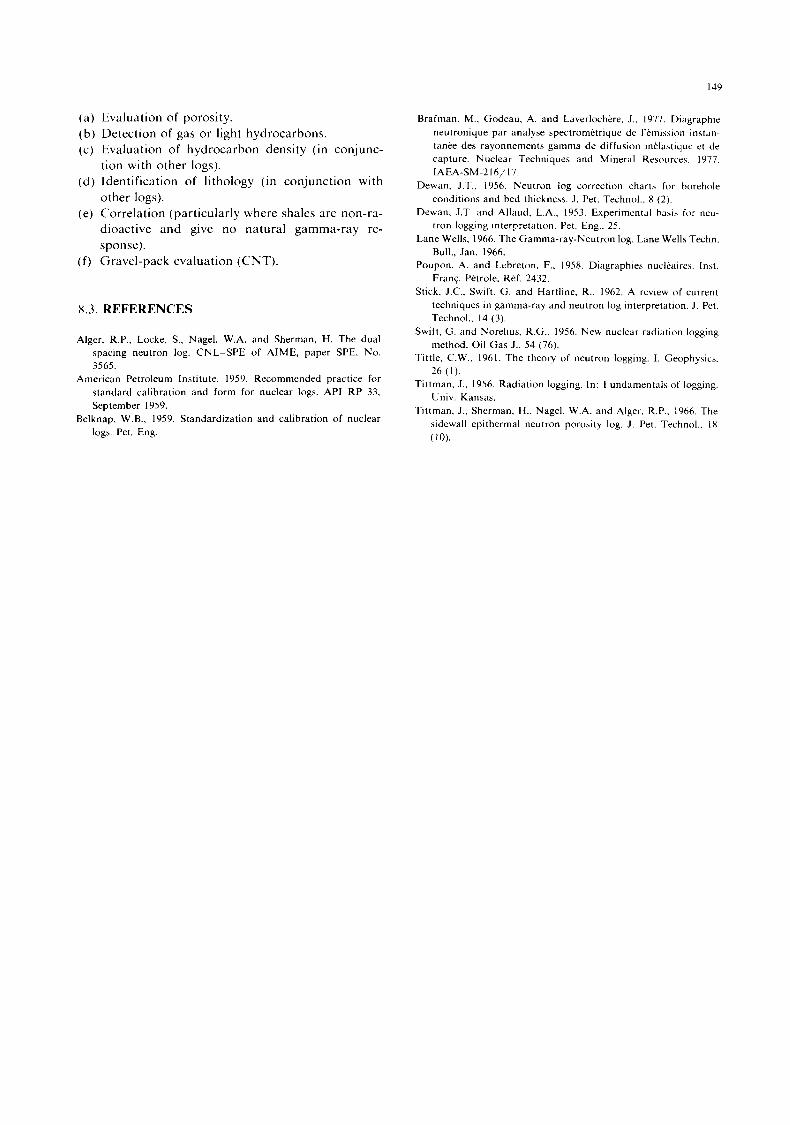
I49
(a) Evaluation of porosity. (b) Detection of gas or light hydrocarbons. (c) Evaluation of hydrocarbon density (in conjunc-
tion with other logs). (d) Identification of lithology (in conjunction with
other logs). (e) Correlation (particularly where shales are non-ra-
dioactive and give no natural gamma-ray re- sponse).
( f ) Gravel-pack evaluation (CNT).
8.3. REFERENCES
Alger, R.P., Locke, S., Nagel, W.A. and Sherman, H. The dual spacing neutron log. CNL-SPE of AIME, paper SPE. No. 3565.
American Petroleum Institute, 1959. Recommended practice for standard calibration and form for nuclear logs. API R P 33, September 1959.
Belknap. W.B., 1959. Standardization and calibration of nuclear logs. Pet. Eng.
Brafman, M., Godeau. A. and Laverlochere, J.. 1977. Diagraphie neutronique par analyse spectrometrique de I’emission instan- tanee des rayonnements gamma d e diffusion inelaatique et de capture. Nuclear Techniques and Mineral Resourcea. 1977. IAEA-SM-2 16/17.
Dewan. J.T., 1956. Neutron log correction charts fo r borehole conditions and bed thickness. J. Pet. Technol.. 8 ( 2 ) .
Dewan. J.T. and Allaud, L.A.. 1953. Experimental hasis f o r neu- tron logging interpretation. Pet. Eng., 25.
Lane Wells, 1966. The Gamma-ray-Neutron log. Lane Wells Techn. Bull., Jan. 1966.
Poupon, A. and Lehreton. F., 1958. Diagraphles nucleairea. Inst. Franq. Petrole. Ref. 2432.
Stick, J.C., Swift, G. and Hartline. R.. 1962. A review of current techniques in gamma-ray and neutron log interpretation. J. Pet. Technol.. 14 (3).
Swift, G. and Norelius. R.G.. 1956. New nuclear radiation logging method. Oil Gas J., 54 (76).
Tittle, C.W., 1961. The theory of neutron logging. I. Geophysics. 26 ( I ) .
Tittman. J., 1956. Radiation logging. In: Fundamentals of logging. Univ. Kansas.
Tittman. J., Sherman, H., Nagel. W.A. and Alger, R.P.. 1966. The sidewall epithermal neutron porosity log. J. Pet. Technol.. 18
( 10).

This Page Intentionally Left Blank
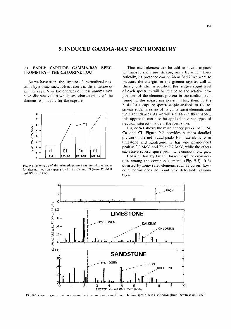
151
9. INDUCED GAMMA-RAY SPECTROMETRY
9.1. EARLY CAPTURE GAMMA-RAY SPEC- TROMETRY-THE CHLORINE LOG
As we have seen, the capture of thermalized neu- trons by atomic nuclei often results in the emission of gamma rays. Now the energies of these gamma rays have discrete values which are characteristic of the element responsible for the capture.
8
7
Fig. 9-1. Schematic of the principle gamma ray emission energies for thermal neutron capture by H. Si. Ca and CI (from Waddell and Wilson. 1959).
Thus each element can be said to have a capture gamma-ray signature (its spectrum), by which. theo- retically, its presence can be identified if we were to measure the energies of the gamma rays as well as their count-rate. In addition, the relative count level of each spectrum will be related to the relative pro- portions of the elements present in the medium sur- rounding the measuring system. This, then, is the basis for a capture spectroscopic analysis of the re- servoir rock, in terms of its constituent elements and their abundances. As we will see later in this chapter, this approach can also be applied to other types of neutron interactions with the formation.
Figure 9-1 shows the main energy peaks for H, Si, Ca and C1. Figure 9-2 provides a more detailed picture of the individual peaks for these elements in limestone and sandstone. H has one pronounced peak at 2.2 MeV, and Fe at 7.7 MeV, while the others each have several quite prominent emission energies.
Chlorine has by far the largest capture cross-sec- tion among the common elements (Fig. 9-3). It is dwarfed by some rarer elements such as boron; how- ever, boron does not emit any detectable gamma rays.
Fig. 9-2. Capture gamma emission from limestone and quartz sandstone. The iron spectrum is also shown (from Dewan et al., 1961)
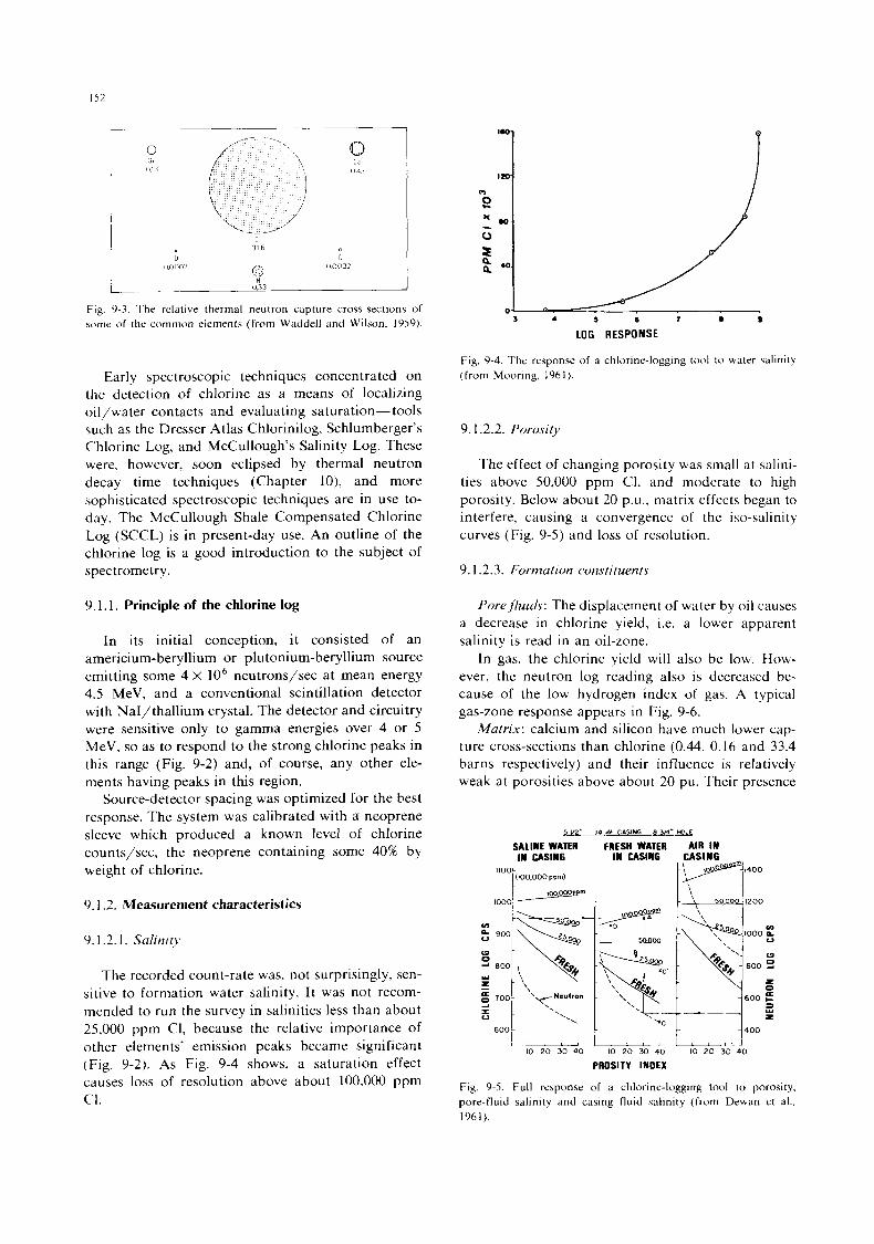
I52
H I 0.33 I Fig. 9-3. The relative thermal neutron capture cross-sections of some of the common elements (from Waddell and Wilson. 1959).
Early spectroscopic techniques concentrated on the detection of chlorine as a means of localizing oil/water contacts and evaluating saturation- tools such as the Dresser Atlas Chlorinilog, Schlumberger's Chlorine Log, and McCullough's Salinity Log. These were, however, soon eclipsed by thermal neutron decay time techniques (Chapter lo), and more sophisticated spectroscopic techniques are in use to- day. The McCullough Shale Compensated Chlorine Log (SCCL) is in present-day use. An outline of the chlorine log is a good introduction to the subject of spectrometry.
9.1.1. Principle of the chlorine log
In its initial conception, it consisted of an americium-beryllium or plutonium-beryllium source emitting some 4 x lo6 neutrons/sec at mean energy 4.5 MeV, and a conventional scintillation detector with NaI/thallium crystal. The detector and circuitry were sensitive only to gamma energies over 4 or 5 MeV, so as to respond to the strong chlorine peaks in this range (Fig. 9-2) and, of course, any other ele- ments having peaks in this region.
Source-detector spacing was optimized for the best response. The system was calibrated with a neoprene sleeve which produced a known level of chlorine counts/sec, the neoprene containing some 40% by weight of chlorine.
9. I .2. Measurement characteristics
9.1.2.1. Salinity
The recorded count-rate was, not surprisingly, sen- sitive to formation water salinity. I t was not recom- mended to run the survey in salinities less than about 25,000 ppm CI, because the relative importance of other elements' emission peaks became significant (Fig. 9-2). As Fig. 9-4 shows, a saturation effect causes loss of resolution above about 100,000 pprn c1.
0 3 4 5 6 7 a 9
LOG RESPONSE
Fig. 9-4. The response of a chlorine-logging tool to water salinity (from Mooring, 1961).
9.1.2.2. Porosity
The effect of changing porosity was small at salini- ties above 50,000 pprn CI, and moderate to high porosity. Below about 20 P.u., matrix effects began to interfere, causing a convergence of the iso-salinity curves (Fig. 9-5) and loss of resolution.
9.1.2.3. Formation constituents
Porefluids: The displacement of water by oil causes a decrease in chlorine yield, i.e. a lower apparent salinity is read in an oil-zone.
In gas, the chlorine yield will also be low. How- ever, the neutron log reading also is decreased be- cause of the low hydrogen index of gas. A typical gas-zone response appears in Fig. 9-6.
Matrix: calcium and silicon have much lower cap- ture cross-sections than chlorine (0.44, 0.16 and 33.4 barns respectively) and their influence is relatively weak at porosities above about 20 pu. Their presence
5 V2" 14 # CASING 8 9 4 ' W L E
SALINE WATER I N CASING
~100.000 ppm)
- 10 20 30 40
FRESH WATER I N CASING
.O I 09
- I0 20 30 40
AIR IN p-l"oo CASING
4 4 0 0
I 10 20 30 40
PROSITV INDEX
Fig. 9-5. Full response of a chlorine-logging tool to porosity. pore-fluid salinity and casing fluid salinity (from Dewan et al.. 1961).
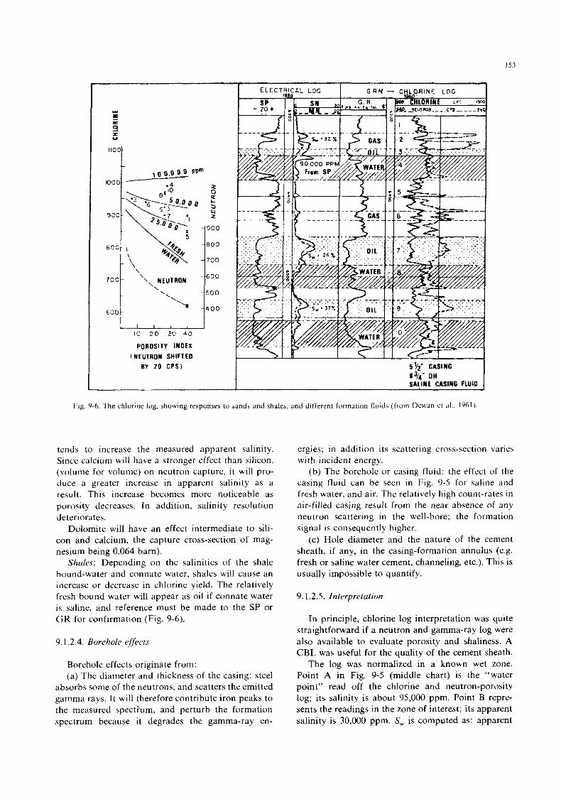
I53
1000
w L- a
2 u
- 1 0 0.0 0 0 ppm
.4 2 --
700-
630
I0 2 0 3 0 4 0
POROSITY I N D E X
I NEUTRON SHIFTED
BY 2 0 C P S )
- \ \
- 630
\ - 500
- ‘‘\ -400
‘, NEUTRON ‘
\ -
Fig. 9-6. The chlorine log. showing responses to sands and shales. and different formation fluids (from D w a n et al.. 1961)
tends to increase the measured apparent salinity. Since calcium will have a stronger effect than silicon, (volume for volume) on neutron capture, i t will pro- duce a greater increase in apparent salinity as a result. This increase becomes more noticeable as porosity decreases. In addition, salinity resolution deteriorates.
Dolomite will have an effect intermediate to sili- con and calcium, the capture cross-section of mag- nesium being 0.064 barn).
Shules: Depending on the salinities of the shale bound-water and connate water, shales will cause an increase or decrease in chlorine yield. The relatively fresh bound water will appear as oil if connate water is saline, and reference must be made to the SP or G R for confirmation (Fig. 9-6).
9.1.2.4. Borehole effects
Borehole effects originate from: (a) The diameter and thickness of the casing: steel
absorbs some of the neutrons, and scatters the emitted gamma rays. I t will therefore contribute iron peaks to the measured spectium, and perturb the formation spectrum because it degrades the gamma-ray en-
ergies; in addition its scattering cross-section varies with incident energy.
(b) The borehole or casing fluid: the effect of the casing fluid can be seen in Fig. 9-5 for saline and fresh water, and air. The relatively high count-rates in air-filled casing result from the near absence of any neutron scattering in the well-bore; the formation signal is consequently higher.
(c) Hole diameter and the nature of the cement sheath, if any, in the casing-formation annulus (e.g. fresh or saline water cement, channeling, etc.). This is usually impossible to quantify.
9.1.2.5. Interpretation
In principle, chlorine log interpretation was quite straightforward if a neutron and gamma-ray log were also available to evaluate porosity and shaliness. A CBL was useful for the quality of the cement sheath.
The log was normalized in a known wet zone. Point A in Fig. 9-5 (middle chart) is the “water point” read off the chlorine and neutron-porosity log; its salinity is about 95,000 ppm. Point B repre- sents the readings in the zone of interest; its apparent salinity is 30,000 ppm. S, is computed as: apparent
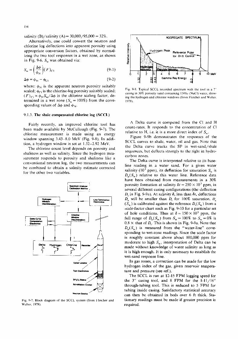
I54
salinity (B)/salinity (A) = 30,000/95,000 = 32%. Alternatively, one could convert the neutron and
chlorine log deflections into apparent porosity using appropriate conversion factors, obtained by normal- izing the two tool responses in a wet zone, as shown in Fig. 9-6. S, was obtained via:
(9-1)
where: G N is the apparent neutron porosity suitably scaled; +,-, is the chlorine-log porosity suitably scaled; ( F),- l = +,S,/A+ is the chlorine scaling factor, de- termined in a wet zone ( S , = 100%) from the corre- sponding values of A+ and G N .
9.1.3. The shale compensated chlorine log (SCCL)
Fairly recently, an improved chlorine tool has been made available by McCullough (Fig. 9-7). The chlorine measurement is made using an energy window spanning 3.43-8.0 MeV (Fig. 9-8). In addi- tion, a hydrogen window is set at 1.32-2.92 MeV.
The chlorine count level depends on porosity and shaliness as well as salinity. Since the hydrogen mea- surement responds to porosity and shaliness like a conventional neutron log, the two measurements can be combined to obtain a salinity estimate corrected for the other two variables.
I / I I
sclntlll*b cry.ul
Neutm Savra ’A Fig. 9-7. Block diagram of the SCCL system (from Fletcher and Walter, 1978).
w WGREGATE SPECTR
Fig. 9-8. Typical SCCL recorded spectrum with the tool in a 7” casing in 30% porosity sand containing 150%0 (NaCI) water. show- ing the hydrogen and chlorine windows (from Fletcher and Walter. 1978).
A Delta curve is computed from the CI and H count-rates. It responds to the concentration of CI relative to H, i.e. i t is a more direct index of S,.
Figure 9-9b demonstrates the responses of the SCCL curves to shale, water, oil and gas. Note that the Delta curve tracks the SP in wet-sand/shale sequences, but deflects strongly to the right in hydro- carbon zones.
The Delta curve is interpreted relative to its base- line reading in a water sand. For a given water salinity (lo3 ppm), its deflection for saturation S, is D,(S,) relative to this water line. Reference data have been obtained from measurements in a 30% porosity formation at salinity St = 250 x lo3 ppm, in several different casing configurations (the deflection D, in Fig. 9-9a). At salinity 8, less than S t , deflections D, will be smaller than D, for 100% saturation. 0, (S,) is calibrated against the reference D,( S,) from a scale-factor chart such as Fig. 9-10 for a particular set of hole conditions. Thus at 6 = 150 X lo3 ppm, the full range of D,(S,) from S, = 100% to S, = 0% is 0.8 x that of 0,. Thls is shown in Fig. 9-9a. Note that D,( S,) is measured from the “water-line’’ corre- sponding to wet-zone readings. Since the scale factor is roughly constant above about 100,000 ppm for moderate to high S,, interpretation of Delta can be made without knowledge of water salinity as long as it is high enough. It is only necessary to establish the wet-sand response line.
In gas zones, a correction can be made for the low hydrogen index of the gas, gwen reservoir tempera- ture and pressure (see ref.).
The SCCL is run at 12-15 FPM logging speed for the 3” casing tool, and 8 FPM for the 1-1 1/16” through-tubing tool. This is reduced to 5 FPM for tubing inside casing. Satisfactory statistical accuracy can then be obtained in beds over 6 f t thick. Sta- tionary readings must be made if greater precision is required.
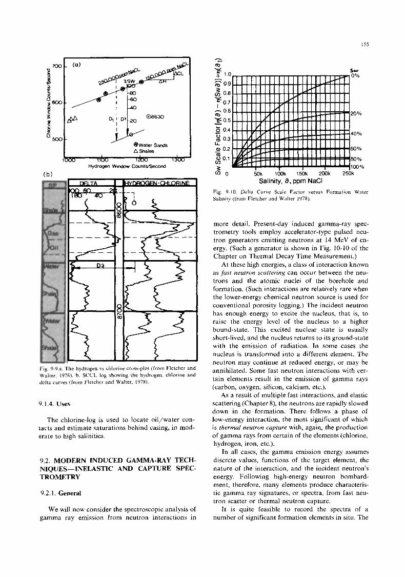
@water sands A Shales
1 m 1 1 0 0 Hydrogen Window CcuntVSecond
Fig. 9-10, Delta Curve Scale Factor versus Formation Water Salinity (from Fletcher and Walter 1978).
Fig. 9-92. The hydrogen vs chlorine cross-plot (from Fletcher and Walter, 1978). b. SCCL log showing the hydrogen, chlorine and delta curves (from Fletcher and Walter, 1978).
9.1.4. Uses
The chlorine-log is used to locate oil/water con- tacts and estimate saturations behind casing, in mod- erate to high salinities.
9.2. MODERN INDUCED GAMMA-RAY TECH- NIQUES-INELASTIC AND CAPTURE SPEC- TROMETRY
9.2.1. General
We will now consider the spectroscopic analysis of gamma ray emission from neutron interactions in
more detail. Present-day induced gamma-ray spec- trometry tools employ accelerator-type pulsed neu- tron generators emitting neutrons at 14 MeV of en- ergy. (Such a generator is shown in Fig. 10-10 of the Chapter on Thermal Decay Time Measurement.)
At these high energies, a class of interaction known as fast neutron scattering can occur between the neu- trons and the atomic nuclei of the borehole and formation. (Such interactions are relatively rare when the lower-energy chemical neutron source is used for conventional porosity logging.) The incident neutron has enough energy to excite the nucleus, that is, to raise the energy level of the nucleus to a higher bound-state. This excited nuclear state is usually short-lived, and the nucleus returns to its ground-state with the emission of radiation. In some cases the nucleus is transformed into a different element. The neutron may continue at reduced energy, or may be annihilated. Some fast neutron interactions with cer- tain elements result in the emission of gamma rays (carbon, oxygen, silicon, calcium, etc.).
As a result of multiple fast interactions, and elastic scattering (Chapter 8), the neutrons are rapidly slowed down in the formation. There follows a phase of low-energy interaction, the most significant of which is thermal neutron capture with, again, the production of gamma rays from certain of the elements (chlorine, hydrogen, iron, etc.).
In all cases, the gamma emission energy assumes discrete values, functions of the target element, the nature of the interaction, and the incident neutron’s energy. Following high-energy neutron bombard- ment, therefore, many elements produce characteris- tic gamma ray signatures, or spectra, from fast neu- tron scatter or thermal neutron capture.
It is quite feasible to record the spectra of a number of significant formation elements in situ. The
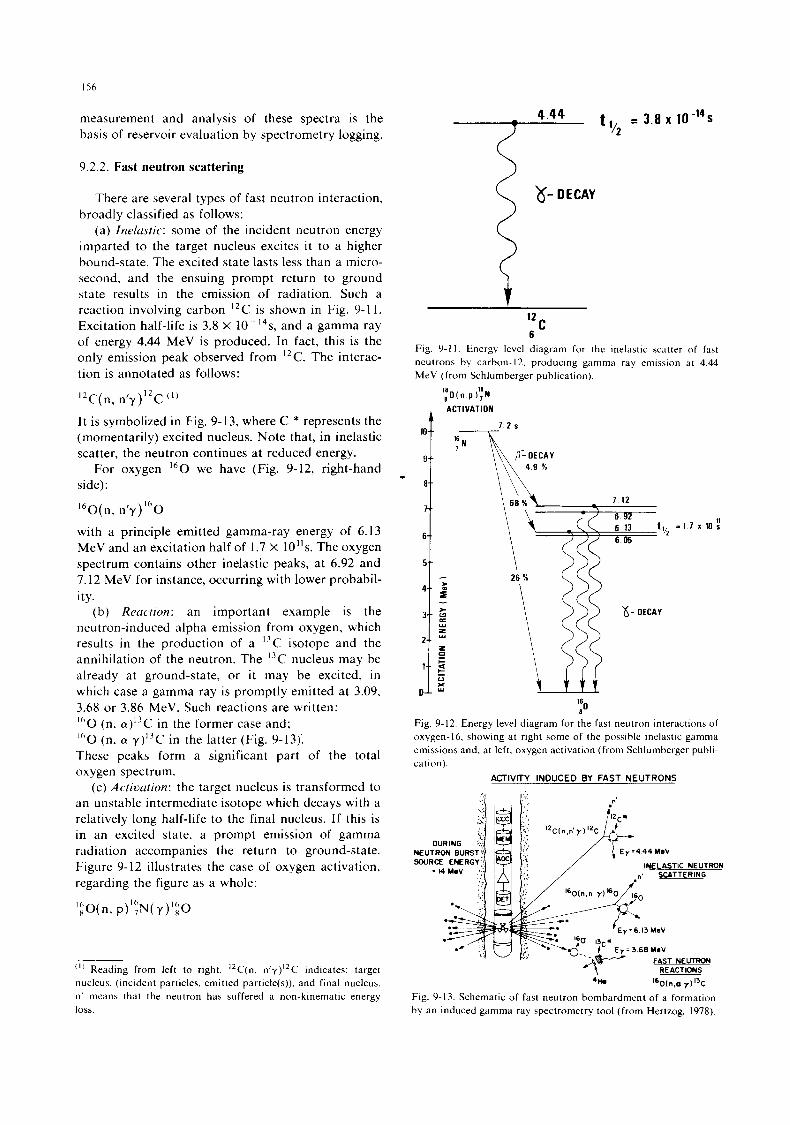
156
measurement and analysis of these spectra is the basis of reservoir evaluation by spectrometry logging.
9.2.2. Fast neutron scattering
There are several types of fast neutron interaction, broadly classified as follows:
(a) Inekustic: some of the incident neutron energy imparted to the target nucleus excites it to a higher bound-state. The excited state lasts less than a micro- second, and the ensuing prompt return to ground state results in the emission of radiation. Such a reaction involving carbon "C is shown in Fig. 9-1 1. Excitation half-life is 3.8 X 10-l4s, and a gamma ray of energy 4.44 MeV is produced. In fact, this is the only emission peak observed from "C. The interac- tion is annotated as follows:
l2C(n, n fy ) I2c ( I )
It is symbolized in Fig. 9-13, where C * represents the (momentarily) excited nucleus. Note that, in inelastic scatter, the neutron continues at reduced energy.
For oxygen 160 we have (Fig. 9-12, right-hand side):
I60(n, n'y)I60
with a principle emitted gamma-ray energy of 6.13 MeV and an excitation half of 1.7 X 10"s. The oxygen spectrum contains other inelastic peaks, at 6.92 and 7.12 MeV for instance, occurring with lower probabil- ity.
(b) Reuction: an important example is the neutron-induced alpha emission from oxygen, which results in the production of a I3C isotope and the annihilation of the neutron. The "C nucleus may be already at ground-state, or it may be excited, in which case a gamma ray is promptly emitted at 3.09, 3.68 or 3.86 MeV. Such reactions are written: 0 (n, a)"C in the former case and;
IhO (n, (Y y)I3C in the latter (Fig. 9-13): These peaks form a significant part of the total oxygen spectrum.
(c) Activation: the target nucleus is transformed to an unstable intermediate isotope which decays with a relatively long half-life to the final nucleus. If this is in an excited state, a prompt emission of gamma radiation accompanies the return to ground-state. Figure 9-12 illustrates the case of oxygen activation, regarding the figure as a whole:
I6
' I ' Reading from left to right, "C(n, n'y)' 'C indicates: target nucleus. (incident particles, emitted particle(s)). and final nucleus. 11' means that the neutron has suffered a non-kinematic energy loss.
-y- t 1,2 = 3.8 x 10-l4s
C 12
6 Fig. 9-1 1 . Energy level diagram for the inelastic scatter o f fast neutrons by carbon-12. produclng gamma ray emission at 4.44 MeV (from Schlumberger publication).
';O(n.p#YN
, ACTIVATION
= 1 7 x 10.:
Fig. 9-12. Energy level diagram for the fast neutron interactions of oxygen-16, showing at right 5ome of the possihle inelastic gamma emissions and, at left. oxygen activation (from Schlumberger publi- cation).
ACTIVITY INDUCED BY FAST NEUTRONS
NEUTRON BURST
SOURCE ENERGY INELASTIC NEUTRON
4na '%(n.a y)"t Fig. 9-13. Schematic of fast neutron bombardment of a formation by an induced gamma ray spectrometry tool (from Hertzog. 1978).
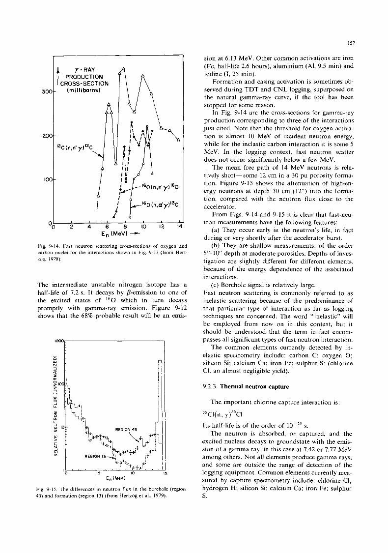
157
y - RAY PRODUCTION
CROSS-SECTION (mi II i barns)
t h 1 I I I 1 I 1
2 4 6 8 10 12 Id En (MeV) -
Fig. 9-14. Fast neutron scattering cross-sections of oxygen and carbon nuclei for the interactions shown in Fig. 9-13 (from Hert- zog, 1978).
The intermediate unstable nitrogen isotope has a half-life of 7.2 s. It decays by p-emission to one of the excited states of I6O which in turn decays promptly with gamma-ray emission. Figure 9- 12 shows that the 68% probable result will be an emis-
En (MeV)
Fig. 9-15. The differences in neutron flux in the borehole (region 43) and formation (region 13) (from Hertzog et al., 1979).
sion at 6.13 MeV. Other common activations are iron (Fe, half-life 2.6 hours), aluminium (Al, 9.5 min) and iodine (I, 25 min).
Formation and casing activation is sometimes ob- served during TDT and CNL logging, superposed on the natural gamma-ray curve, if the tool has been stopped for some reason.
In Fig. 9-14 are the cross-sections for gamma-ray production corresponding to three of the interactions just cited. Note that the threshold for oxygen activa- tion is almost 10 MeV of incident neutron energy, while for the inelastic carbon interaction i t is some 5 MeV. In the logging context, fast neutron scatter does not occur significantly below a few MeV.
The mean free path of 14 MeV neutrons is rela- tively short-some 12 cm in a 30 pu porosity forma- tion. Figure 9-15 shows the attenuation of high-en- ergy neutrons at depth 30 cm (12”) into the forma- tion, compared with the neutron flux close to the accelerator.
From Figs. 9-14 and 9-15 i t is clear that fast-neu- tron measurements have the following features:
(a) They occur early in the neutron’s life, in fact during or very shortly after the accelerator burst.
(b) They are shallow measurements; of the order 5”- 10” depth at moderate porosities. Depths of inves- tigation are slightly different for different elements, because of the energy dependence of the assbciated interactions.
Fast neutron scattering is commonly referred to as inelastic scattering because of the predominance of that particular type of interaction as far as logging techniques are concerned. The word “inelastic” will be employed from now on in this context, but it should be understood that the term in fact encom- passes all significant types of fast neutron interaction.
The common elements currently detected by in- elastic spectrometry include: carbon C; oxygen 0; silicon Si; calcium Ca; iron Fe; sulphur S: (chlorine C1, an almost negligible yield).
(c) Borehole signal is relatively large.
9.2.3. Thermal neutron capture
The important chlorine capture interaction is:
3 5 ~ i ( n , v ) 3 6 ~ i
Its half-life is of the order of 10p20s. The neutron is absorbed, or captured, and the
excited nucleus decays to groundstate with the emis- sion of a gamma ray, in this case at 7.42 or 7.77 MeV among others. Not all elements produce gamma rays, and some are outside the range of detection of the logging equipment. Common elements currently mea- sured by capture spectrometry include: chlorine C1; hydrogen H; silicon Si; calcium Ca; iron Fe; sulphur S.
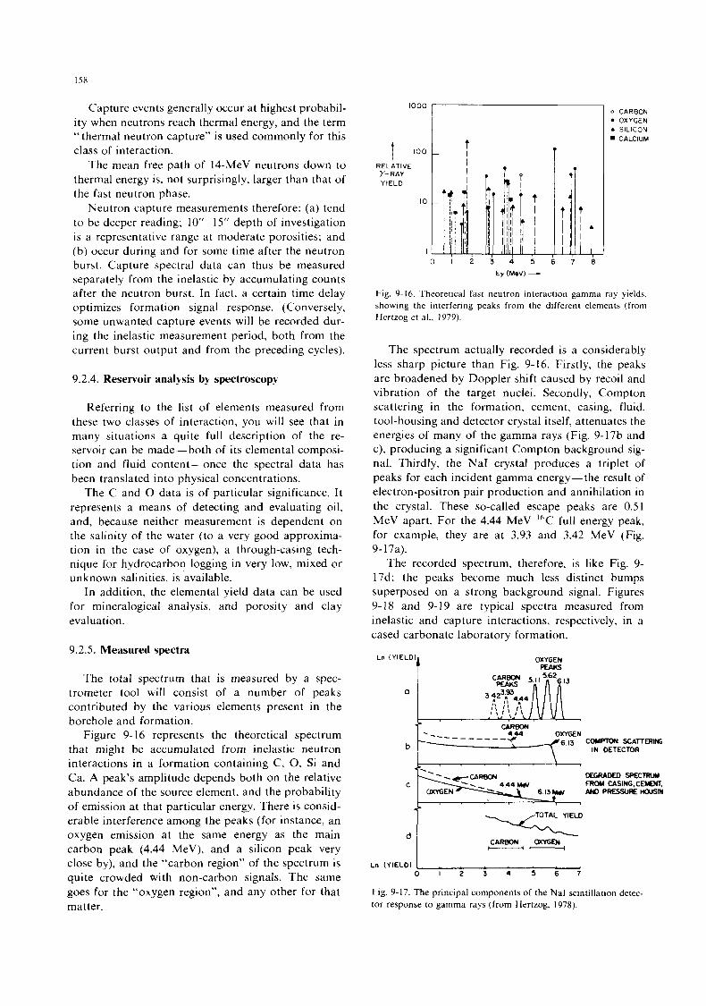
158
Capture events generally occur at highest probabil- ity when neutrons reach thermal energy, and the term “thermal neutron capture” is used commonly for this class of interaction.
The mean free path of 14-MeV neutrons down to thermal energy is, not surprisingly, larger than that of the fast neutron phase.
Neutron capture measurements therefore: (a) tend to be deeper reading; 10”-15” depth of investigation is a representative range at moderate porosities; and (b) occur during and for some time after the neutron burst. Capture spectral data can thus be measured separately from the inelastic by accumulating counts after the neutron burst. In fact, a certain time delay optimizes formation signal response. (Conversely, some unwanted capture events will be recorded dur- ing the inelastic measurement period, both from the current burst output and from the preceding cycles).
9.2.4. Reservoir analysis by spectroscopy
Referring to the list of elements measured from these two classes of interaction, you will see that in many situations a quite full description of the re- servoir can be made-both of its elemental composi- tion and fluid content-once the spectral data has been translated into physical concentrations.
The C and 0 data is of particular significance. It represents a means of detecting and evaluating oil, and, because neither measurement is dependent on the salinity of the water (to a very good approxima- tion in the case of oxygen), a through-casing tech- nique for hydrocarbon logging in very low, mixed or unknown salinities, is available.
I n addition, the elemental yield data can be used for mineralogical analysis, and porosity and clay evaluation.
9.2.5. Measured spectra
The total spectrum that is measured by a spec- trometer tool will consist of a number of peaks contributed by the various elements present in the borehole and formation.
Figure 9- 16 represents the theoretical spectrum that might be accumulated from inelastic neutron interactions in a formation containing C, 0, Si and Ca. A peak’s amplitude depends both on the relative abundance of the source element, and the probability of emission at that particular energy. There is consid- erable interference among the peaks (for instance, an oxygen emission at the same energy as the main carbon peak (4.44 MeV), and a silicon peak very close by), and the “carbon region” of the spectrum is quite crowded with non-carbon signals. The same goes for the “oxygen region”, and any other for that matter.
RELATIVE 7- RAY YIELD
10
I
0 1 2 3 4 5 6
E y (MeV) 4
0 CARBON OXYGEN
A SILICON CALCIUM
Fig. 9-16. Theoretical fast neutron interaction gamma ray yields. showing the interfering peaks from the different elements (from Hertzog et a].. 1979).
The spectrum actually recorded is a considerably less sharp picture than Fig. 9-16. Firstly, the peaks are broadened by Doppler shift caused by recoil and vibration of the target nuclei. Secondly, Compton scattering in the formation, cement, casing, fluid, tool-housing and detector crystal itself, attenuates the energies of many of the gamma rays (Fig. 9-17b and c), producing a significant Compton background sig- nal. Thirdly, the NaI crystal produces a triplet of peaks for each incident gamma energy-the result of electron-positron pair production and annihilation in the crystal. These so-called escape peaks are 0.51 MeV apart. For the 4.44 MeV “C full energy peak, for example, they are at 3.93 and 3.42 MeV (Fig. 9- 17a).
The recorded spectrum, therefore, is like Fig. 9- 17d; the peaks become much less distinct bumps superposed on a strong background signal. Figures 9-18 and 9-19 are typical spectra measured from inelastic and capture interactions, respectively, in a cased carbonate laboratory formation.
OXYGEN PEAW
+ ” ” CARBON . 444 6 13 C O W ” SCAfTERIffi
IN DETECTOR
--- - _ - _ _ _ _ b
I
i] TOTAL YIELD
\ CARBON WXGEN --
Ln (YIELD) I . , . ~ . . , 0 1 2 3 4 5 6 7
Fig. 9-17. The principal components of the NaI scintillation detec- tor response to gamma rays (from Hertzog, 1978).
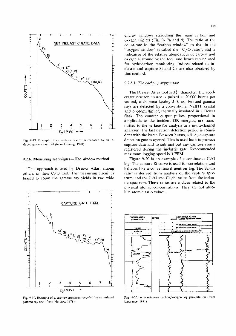
159
r NET INELASTIC GATE DATA
1 2 3 4 5 6 7 8 1 I I I I I I I
Ey (MeV) - Fig. 9-18. Example of an inelastic spectrum recorded by an in- duced gamma ray tool (from Hertzog, 1978).
9.2.6. Measuring techniques-The window method
This approach is used by Dresser Atlas, among others, in their C/O tool. The measuring circuit is biased to count the gamma ray yields in two wide
ti
E,.(MeV) -+
Fig. 9-19. Example of a capture spectrum recorded by an induced gamma ray tool (from Hertzog, 1978).
energy windows straddling the main carbon and oxygen triplets (Fig. 9-17a and d). The ratio of the count-rate in the “carbon window” to that in the “oxygen window” is called the “C/O ratio”. and is indicative of the relative abundances of carbon and oxygen surrounding the tool, and hence can be used for hydrocarbon monitoring. Indices related to in- elastic and capture Si and Ca are also obtained by this method.
9.2.6.1. The carbon/oxygen tool
The Dresser Atlas tool is 3;“ diameter. The accel- erator neutron source is pulsed at 20,000 bursts per second, each burst lasting 5-8 ps. Emitted gamma rays are detected by a conventional NaI(T1) crystal and photomultiplier, thermally insulated in a Dewar flask. The counter output pulses, proportional in amplitude to the incident GR energies, are trans- mitted to the surface for analysis in a multi-channel analyzer. The fast neutron detection period is coinci- dent with the burst. Between bursts, a 5-8 ps capture detection gate is opened. This is used both to provide capture data and to subtract out any capture events registered during the inelastic gate. Recommended maximum logging speed is 3 FPM.
Figure 9-20 is an example of a continuous C/O log. The capture Si curve is used for correlation, and behaves like a conventional neutron log. The Si/Ca ratio is derived from analysis of the capture spec- trum, and the C/O and Ca/Si ratios from the inelas- tic spectrum. These ratios are indices related to the physical atomic concentrations. They are not abso- lute atomic ratio values.
Fig. 9-20. A continuous carbon/oxygen log presentation (from Lawrence, 1981).
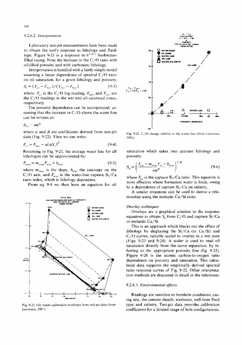
I60
9.2.6.2. Interpretation IF. - F A ICNCUUTED)
F.. f 8F. - 2 5 1
Laboratory test-pit measurements have been made to obtain the tool's response to lithology and fluid- type. Figure 9-21 is a response in 65/x" freshwater- filled casing. Note the increase in the C/O ratio with oil-filled porosity and with carbonate lithology.
Interpretation is handled with a fairly simple model assuming a linear dependence of spectral C/O ratio on oil saturation, for a given lithology and porosity.
s,, = ( F,,, - F,,,, >A 4,<, - F,,,, (9-3) where: t,, is the C/O log reading, F,.,,,, and e,,,, are the C/O readings in the wet and oil-saturated zones, respectively.
The porosity dependence can be incorporated. as- suming that the increase in C/O above the water line can be written as:
A,,, = a@
where a and p are coefficients derived from test-pit data (Fig. 9-22). Then we can write:
F,.,, = F,,,, + 4 @S<, > D (9-4) Returning to Fig. 9-21, the average water line for all lithologies can be approximated by:
Fw,, = mwscFwsc + bws, (9-5) where mwsc is the slope, bws, the intercept on the C/O axis, and F,,, is the water-line capture Si/Ca ratio index, which is lithology dependent.
From eq. 9-4 we then have an equation for oil
CIO .. SUC.
T
(OIL-WATER ENVELOPE SIZE VS POROSITVI TEST PIT DATA. 8W CASING
FRESH WATER
I, \
0 WATERSAND
OILSAND
A OIL LIME
0 WATER DOLOMITE
WATERLIME
\ OIL LINES
SUCa RATW
Fig. 9-21. Oil/water calibration envelopes from test-pit data (from Lawrence, 1981).
Rxcsllv TEST M DATA. W uIs*yo
FRESU WATER
WATER SAND
OIL SAND WATER LlYE
A OIL LIME
WATER DOLOWTE
t OIL L"7 '
0.t /
WATERLINE 0
O W T - k 7 2 %
POROSITY (PERCENT)
-05
Fig. 9-22. C/O change relative to the water line (from Laurence. 1981).
saturation which takes into account lithology and porosity:
(9-6)
where F,, is the capture Si/Ca ratio. This equation is most effective where formation water is fresh, owing to a dependence of capture Si/Ca on salinity.
A similar treatment can be used to derive a rela- tionshp using the inelastic Ca/Si ratio.
Overlay techniques Overlays are a graphcal solution to the response
equations to obtain So from C/O and capture Si/Ca or inelastic Ca/Si.
T h s is an approach which blacks out the effect of lithology by displaying the Si/Ca (or Ca/Si) and C/O curves, suitably scaled to overlay in a wet zone (Figs. 9-23 and 9-24). A scaler is used to read oil saturation directly from the curve separation, by re- ferring to the appropriate porosity line (fig. 9-25). Figure 9-26 is the atomic carbon-to-oxygen ratio dependence on porosity and saturation. This calcu- lated data supports the empirically derived spectral ratio response curves of Fig. 9-22. Other interpreta- tion methods are discussed in detail in the references.
9.2.6.3. Environmental effects
Readings are sensitive to borehole conditions, cas- ing size, the cement sheath, washouts, well-bore fluid type and salinity. Test-pit data provides calibration coefficients for a limited range of hole configurations.
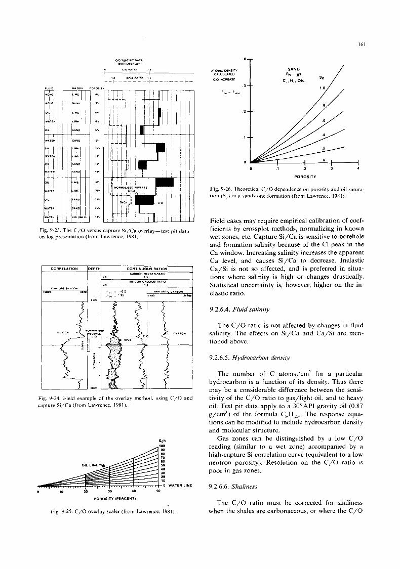
161
CORRELATION
.4 T
DEPTH CONTINUOUS RATIOS c m m m O X V G E W I A T ! ~
SILICON CALCIUM n.mo 1 0 I 5
T
~
I I
i I
~
t , t
L Flg. 9-23. The C/O versus capture Si/Ca overlay-test-pit data on log presentatlon (from Lawrence. 1981).
ATOUIC DENSITI CALCULATED
CNJ INCREASE
F,, - F",,
SAND
c, n., OIL 3 --
2 --
I 0 1 2 3 4
POROSITY
Fig. 9-26. Theoretical C/O dependence on porosity and oil satura- tion (S , ) in a sandstone formation (from Lawrence, 1981).
Field cases may require empirical calibration of coef- ficients by crossplot methods, normalizing in known wet zones, etc. Capture Si/Ca is sensitive to borehole and formation salinity because of the C1 peak in the Ca window. Increasing salinity increases the apparent Ca level, and causes Si/Ca to decrease. Inelastic Ca/Si is not so affected, and is preferred in situa- tions where salinity is high or changes drastically. Statistical uncertainty is, however, higher on the in- elastic ratio.
9.2.6.4. Fluid salinity
The C/O ratio is not affected by changes in fluid salinity. The effects on Si/Ca and Ca/Si are men- tioned above.
9.2.6.5. Hydrocarbon density
The number of C atoms/cm3 for a particular hydrocarbon is a function of its density. Thus there may be a considerable difference between the sensi- tivity of the C/O ratio to gas/light oil, and to heavy oil. Test pit data apply to a 30"API gravity oil (0.87 g/cm3) of the formula C,H,,. The response equa- tions can be modified to include hydrocarbon density and molecular structure.
Gas zones can be distinguished by a low C/O reading (similar to a wet zone) accompanied by a high-capture Si correlation curve (equivalent to a low neutron porosity). Resolution on the C/O ratio is poor in gas zones.
Fig. 9-24. Field example of the overlay method, using C/O and capture Si/Ca (from Lawrence, 1981).
9.2.6.6. Shaliness
POROSITY (PERCENT)
Fig. 9-25. C/O overlay scaler (from Lawrence, 1981). The C/O ratio must be corrected for shaliness
when the shales are carbonaceous, or where the C/O
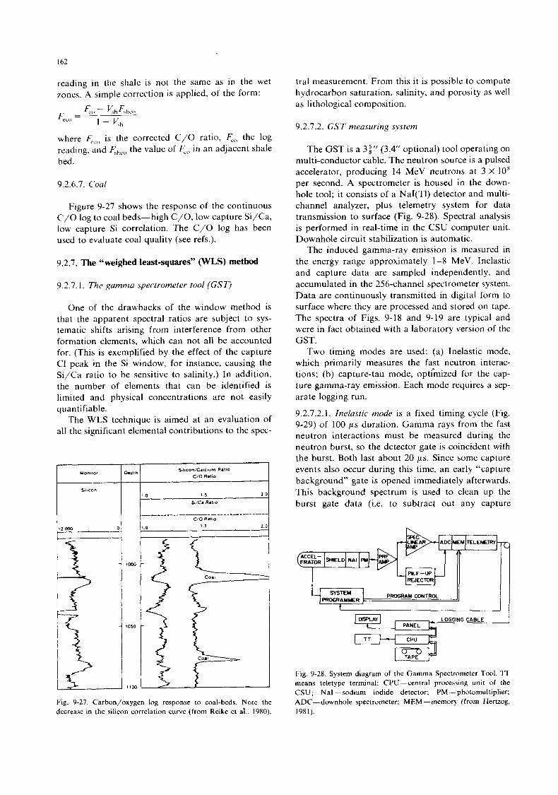
162
M 0 n I ID r
reading in the shale is not the same as in the wet zones. A simple correction is applied, of the form:
S,l,con/C.lcl“m R.140
c/o R.tm Oopln
where F,,,, is the corrected C/O ratio, F,,, the log reading, and qhco the value of F , , in an adjacent shale bed.
9.2.6.1. C o d
Figure 9-27 shows the response of the continuous C/O log to coal beds-high C/O, low capture Si/Ca, low capture Si correlation. The C/O log has been used to evaluate coal quality (see refs.).
9.2.7. The “weighed least-squares” (WLS) method
9.2.7.1. The gumma spectrometer tool (GST)
One of the drawbacks of the window method is that the apparent spectral ratios are subject to sys- tematic shifts arising from interference from other formation elements, which can not all be accounted for. (This is exemplified by the effect of the capture Cl peak in the Si window, for instance, causing the Si/Ca ratio to be sensitive to salinity.) In addition, the number of elements that can be identified is limited and physical concentrations are not easily quantifiable.
The WLS technique is aimed at an evaluation of all the significant elemental contributions to the spec-
Fig. 9-27. Carbon/oxygen log response to coal-beds. Note the decrease in the silicon correlation curve (from Reike et al., 1980).
tral measurement. From this it is possible to compute hydrocarbon saturation, salinity, and porosity as well as lithological composition.
9.2.7.2. GST measuring system
The GST is a 3;‘’ (3.4’ optional) tool operating on multi-conductor cable. The neutron source is a pulsed accelerator, producing 14 MeV neutrons at 3 X 10’ per second. A spectrometer is housed in the down- hole tool; it consists of a NaI(T1) detector and multi- channel analyzer, plus telemetry system for data transmission to surface (Fig. 9-28). Spectral analysis is performed in real-time in the CSU computer unit. Downhole circuit stabilization is automatic.
The induced gamma-ray emission is measured in the energy range approximately 1-8 MeV. Inelastic and capture data are sampled independently, and accumulated in the 256-channel spectrometer system. Data are continuously transmitted in digital form to surface where they are processed and stored on tape. The spectra of Figs. 9-18 and 9-19 are typical and were in fact obtained with a laboratory version of the GST.
Two timing modes are used: (a) Inelastic mode, which primarily measures the fast neutron interac- tions; (b) capture-tau mode, optimized for the cap- ture gamma-ray emission. Each mode requires a sep- arate logging run.
9.2.7.2.1. Inelastic mode is a fixed timing cycle (Fig. 9-29) of 100 p s duration. Gamma rays from the fast neutron interactions must be measured during the neutron burst, so the detector gate is coincident with the burst. Both last about 20 ps. Since some capture events also occur during this time, an early “capture background” gate is opened immediately afterwards. This background spectrum is used to clean up the burst gate data (Le. to subtract out any capture
PROGRAM CONTROL
LOGGING CABLE PANEL
TT
Fig. 9-28. System diagram of the Gamma Spectrometer Tool. TT means teletype terminal; CPU-central processing unit of the CSU ; NaI - sodium iodide detector; PM - photomultiplier; ADC-downhole spectrometer; MEM-memory (from Hertzog, 1981).
163
SPECTRA L BURST BKGNO LATE CAPTURE
NEUTRON BURST
I TIME lusec) INELASTIC MODE I I I
BURST
0 100 I INELASTIC 6 CAPTURE
/ CAPTURE 7 RAY
COUNT RATE
0 20 40 84 100
m:m=m -M BACKGAOUNO NET INELASTIC CAPTURE
SPECTRUM BURST
SPECTRUM SPECTRUM SPECTRUM
Fig. 9-29. GST inelastic mode timing program (from Westaway and Hertzog. 1980).
events), resulting in the “net inelastic spectrum” in the figure.
A “late capture” gate measures formation (and the inevitable borehole) capture events. All three spectra, plus circuit calibration data, are sent uphole for analysis.
9.2.7.2.2. Capture-tau mode allows fast neutron and early borehole-related capture events to die away before the detector gate is opened (Fig. 9-30). The entire gating sequence is dependent on the thermal neutron decay time 7 (see Chapter 10). This is mea- sured simultaneously by a self-adjusting tau-loop working along the same lines as the TDT-K except that the background gate is set during the ninth and tenth cycles, which have no neutron bursts. The effect of varying the detector gate delay as formation T
varies, is to enhance the tool response to the forma- tion, at the expense of borehole signal.
This can be further improved by fitting a boron sleeve to the tool housing to displace well-bore fluid. The highly captive boron causes a very rapid deple- tion of thermal neutrons in the borehole, effectively extinguishing the borehole signal before the detector
gates open. Casing or tubing size may preclude the use of this sleeve.
The capture gate, late background and calibration data are transmitted uphole. The formation T mea- surement is also recorded as a capture cross-section, Z, curve.
9.2.7.2.3. Logging speeds. On the surface, the spectral data are accumulated over 6” of tool travel in con- tinuous logging mode. Every 6” the accumulated data are analyzed, and stored on magnetic tape along with the results of the WLS analysis. Capture-tau mode is usually run at 10 FPM or slower.
Inelastic mode is commonly operated with the tool stationary, in which case data are accumulated over 5 minutes per station. Alternatively, a logging speed of 2-1/2 FPM can be used. To reduce statistical vari- ations, several passes may be averaged.
9.2.7.3. WLS spectral analysis
This is a fitting technique. Reference, or standard, spectra for each of the elements it is required to identify, have been derived from laboratory analysis. Each elemental standard represents what the tool would record if surrounded solely by that element. The set in present use for inelastic spectrometry is shown in Fig. 9-31a and the set for capture spectrom- etry in 9-31b. (Note that the detector crystal’s iodine activation yield must be included in the capture standards, since the objective is to analyse ALL significant components of the spectrum).
At each sampling depth, the CSU computer de- termines which linear combination of these standards best fits the logging spectrum, over almost its entire width. The best fi t is assessed according to a least- squares criterion. Rather than using a “trial” and error” approach to the fitting, each standard has its associated linear estimator (Fig. 9-32) which, when multiplied channel for channel into the accumulated log spectrum, produces the corresponding fractional
GST TIMING PROGRAMS
NEUTRON
BACKGROUNO 81
CAPTURE - 7
SPECTROMETRY
10 12 42 u u l u MULTIPLES OF T -
7 111
61
SIMULTANEOUS
MEASUREMENT
MULTIPLES OF T - TOT EOUATION N1/2 - N, + N, = 0
Fig. 9-30. GST capture-tau mode timing diagram (from Westaway and Hertzog, 1980).
164
INELASTIC 1-1- a
CAPTURE 7 h
GAMMA RAY fWfRGY IMaVl
Fig. 9-31. a. The inelastic WLS fitting standards (from Westaway and Hertzog, 1980). b. The capture WLS fitting standards ifrom Westaway and Hertzog, 1980).
contribution of the element in question. Inelastic spectra are processed basically with the
inelastic standard set, but further cleaning up of residual capture events is possible by incorporation of selected capture standards. Capture spectra are processed with the capture standards. The two analyses are, of course, performed completely inde- pendently.
The outputs of the analysis are the elemental yield
ELEMENT RESPONSE LINEAR ESTIMATORS F U N CT IONS
E Y - OXYGEN
0 4 v
Fig. 9-32. The linear estimators (right) for carbon and oxygen spectral yields, used in the WLS analysis (from Hertzog. 1978).
coefficients. These are the fractions of the total spec- trum that are computed to have been contributed by the various elements. The results of a typical inelastic f i t in a clean oil-bearing sandstone, with water-filled cased hole, might be: C : 0.12 (oil) 0 : 0.28 (water, quartz, cement) Si : 0.25 (quartz, cement) Ca: 0.04 (from the cement) Fe: 0.32 (casing and tool housing) S : - 0.01 (none present) Note that the sum of the yields is, by definition, 1.0. The slightly negative S yield is due to statistical variation about zero. In terms of the fitting, i t means that the best f i t was obtained by subtracting a small fraction of the S standard rather than adding.
From these coefficients, the spectral yield ratios are computed. They were chosen for correlation with the conventional macroscopic reservoir parameters such as porosity and lithology. These yield ratios are listed in Table 9-1.
Other outputs include gate count-rates, various calibration data concerned with the alignment of the downhole circuitry, crystal resolution (peak width, which deteriorates with crystal age), and a quality indicator for the spectral fitting.
All this data goes onto tape along with the spectra.
TABLE 9-1
The GST spectral yield ratios presently output on CSU (from Westaway and Hertzog, 1980).
Yield ratio Interaction Name Label
c/o Inelastic Carbon-oxygen ratio COR CI/H Capture Salinity-indicator ratio SIR H/(Si + Ca) Capture Porosity-indicator ratio PIR Fe/(Si + Ca) Capture Iron-indicator ratio IIR Si/(Si + Ca) Capture and Lithology-indicator ratio LIR
inelastic
I65
STATIONPIRV INELASTIC MODE
COR 0
A
Fig. 9-33. Example of a GST continuous capture-tau mode log (a), and stationary mode inelastic log (b) in a clean carbonate reservoir. Note that the wellbore oil/water interface has moved between runs (adapted from Westaway and Hertzog, 1980).
Selected channels. particularly the yield coefficients, ratios and count-rates, are displayed on film. The spectra can be observed on the viewer of the CSU.
Figure 9-33a is a section of continuous capture-tau log, and Fig. 9-33b the corresponding inelastic mode based on 5-minute stations. The yield ratios are dis- played.
9.2.7.4. Reprocessing of data
Since all the downhole spectra are recorded on tape. i t is possible to re-analyze them i f necessary to improve the results or correct for factors not taken into account in the real-time analysis. Such factors include:
(a) Inclusion of an element not present in the set of standards used, but present in the formation spec- trum.
(b) Exclusion from the standards of any element not present in the formation (i.e. less than 2% contri- bution to the measured spectrum). Minimising the standards used in the W.L.S. fit reduces statistical uncertainty.
(c) The effects of temperature, humidity, age, or damage, on the detector crystal. These tend to de- grade the crystal resolution, i.e. to broaden the peaks, so that the standards no longer are valid because they were obtained using a good crystal. Appropriately degraded standards can be simulated.
(d) Changes in spectrometer alignment. Although
the downhole circuitry is automatically aligned by means of channel calibrating signals, residual shifts or gain errors must be corrected for, because the standard spectra were made with a well-aligned tool.
Much of this corrective processing is now per- formed in real-time in the CSU. Subsequent re- processing can be performed off-line in the CSU or computing centre, should i t be necessary.
9.2.7.5. In terpretation
The relations between the measured spectral yields and physical atomic concentrations depend on neu- tron energy distribution and interaction cross-sec- tions, integrated over all space and over all neutron energies, in addition to the obvious dependence on atomic concentrations. A rigorous treatment of ele- mental yields would produce a response equation of the form (taking elemental carbon as an example):
X c = 1 I#( E, r ) u( E ) V,( r ) d Ed r (9-6 1 E r
where #( E , r ) is the flux of neutrons of energy E at distance r from the source, a( E ) is the total interac- tion cross-section for neutron energy E, and y , ( r ) is the concentration of atoms of carbon at r. Further terms describing the transport of gamma rays from point of emission to detector would also be required.
Thus the elemental yield for carbon, for example, cannot be easily converted to its abundance in the formation. Furthermore, the conversion coefficient would not be the same as for oxygen.
Interpretation of elemental yields or yield ratios is a complex problem, therefore. WLS analysis has the advantage of extracting true spectral fractions from the measured spectrum, rather than apparent ones. making the development of a rigorous interpretation model more feasible.
Induced gamma-ray yield responses are being re- searched using computerized mathematical modelling and laboratory calibrations. A simplified interpreta- tion model has been used on field data with good results. This model assumes that the elemental yields depend in a linear manner on the concentration of elements averaged over the borehole and formation, and the average interaction cross-sections. This ap- proach has been particularly successful in the inter- pretation of the C and 0 yields for hydrocarbon evaluation.
9.2.7.5.1. Hydrocarbon saturations from the C und 0 yields
The ratio spectral carbon yield/spectral oxygen yield (COR) can be approximated by:
166
where: u ~ , u,, are the effective fast neutron interaction cross
sections for C and 0, averaged over all interac- tion types and all neutron energies.
a , /3 are the atomic concentrations of carbon in the rock matrix volume ( 1 - +) and in the hydro- carbon volume +( 1 - &,), respectively.
y . 6 are the atomic concentrations of oxygen in the rock matrix volume ( 1 - +) and the pore water volume +SW, respectively.
B,. Bc, represent carbon and oxygen background con- tributions from the borehole. These are im- portant terms because they are relatively large and cause systematic shifts to the log readings. They depend on hole configuration (size, casing, cement) and hole fluid.
+ is the effective formation porosity, most accurately obtained from open-hole logs.
The equation can be easily modified to include shale terms. Figure 9-34 shows some laboratory data plotted to show the dependence of COR on porosity, hydrocarbon saturation and lithology. The response fans, computed with an appropriate choice of con- stants, in eq. 9-7 f i t the data points closely.
Table 9-2 lists the theoretical a and y matrix carbon and oxygen concentrations for a variety of lithologies, together with the /3 of an oil of density 0.85 g/cm', type C,H,,,, and the 6 of pure water. These constants are easily computed from the bulk density p (g/cm3), gram molecular weight (GMW), and number of atoms per n molecule (in units of Avogadro's number).
Atoms/cm3 = p X n/GMW For example, for pure limestone; CaCO,: a = 2.71
x 1/100 = 0.027; and y = 2.72 x 3/100 = 0.081. For
f , RAT
COR
0 35r
0 30
'020) u+z '/
0 0.1 012 0:3 0.4
c#+ POROSITY - Fig. 9-34. The dependence of the ratio of carbon to oxygen yields (COR) on porosity and water saturation S,, in limestone and sandstone l i thologies. water-filled hole. Both laboratory data and postulated response curves are shown (adapted from Westaway and Hertzog, 1980).
TABLE 9-2
Some atomic densities in units of Avogadro's number (6.023 X lo2' atoms/mole)
Density Oxygen carbon (g/cm3) (atoms/cm3) (atom/cm')
Limestone Dolomite Quartz sandstone Anhydrite Oil Water
Feldspars Microcline Albite Anorthite
Micas Muscovite Biotite Glauconite
Sample I Sample I1
Clays Illite Kaolinite Chlorite Montmorillonite
2.71
2.65 2.96 0.85 1 .o
2.87
2.56 2.62 2.76
2.83 3.08
2.5 1 2.65
2.53 2.42 2.17 2.12
0.08 1 0.027 0.094 0.03 1
0.087 - - 0.06 1 0.056 -
0.088 -
0.074 ~
0.080 -
0.079 -
0.085 -
0.08 1 -
0.074 -
0.075 -
0.082 -
0.084 -
0.082 -
0.077 ~
silica, SO,: a = 0; and y = 2.65 X 2/60 = 0.088. Note that the concentration of atomic oxygen is, unlike any other element, fairly constant in many minerals. This suggests that the COR measurement should be relatively insensitive to variations in non- carbon-bearing mineralogy (tuffites, clays, feldspars, etc.), all other things being equal.
The borehole terms B,, and B, have been derived from laboratory and field data. Most importantly, in water-filled open hole or casing, B, = 0. In oil-filled open-hole B, = 0. In oil-filled cased-hole, both B, (oil) and B, (cement sheath) will be non-zero.
Equation 9-7 defines a unique response curve for a given lithology and hole configuration, resembling a fan graduated in terms of S,. In Fig. 9.-35, four COR vs porosity crossplots are shown to demonstrate this. Figures 9-35a and 9-35b correspond to the oil-filled and water-filled sections of the example log of Fig. 9-33, which is a clean limestone reservoir. Note the change of well-bore fluid from oil to water causes a large downward shift of the COR ratio, and a reduc- tion in the dynamic range (i.e. the spread of the fan from S, = 1 to S, = 0). This example in fact shows two prominent interpretational features: (a) a major oil-water transition in the formation at 4986' and (b) a breakthrough of water above this OWC, 4970-4959'.
These features can also be discerned on the cros- splots. Figure 9-36 presents the CPI analysis of the COR data, compared with 2-derived saturations.
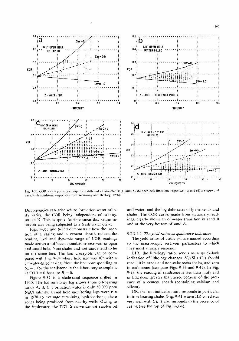
I67
0 . 5 ~ . . . . . . . . . . . . . . . , . . . . . . . . . . . . . . . . . . . . . . . .
;b : 8.5" OPEN HOLE
0.4: .. WATER-FILLED ...... : ......... : ......... :
...................... ......... ......... :
0.4; . . . . . . . . . ............................... 0.1: . . . . . . . . . ...............................
......................................... 0 : . . . . . . . . . :......*,.:*.....".:.. . . * . . , . :
SW=l.O
i z - AXIS FR~OUENCY PLOT i i 2 - AXIS :'SIR
0 0.1 0.2 0.3 0.4 0 0 1 0.2 0 3 0.4
POROSITY POROSITY
0.3
0.2 ...................................................
: Z . A X I S : ~ M A R * Y i : 2- AXIS GAMMA RAY i
p, ................................................... 0 , : . . . . . . . . . . . . . . . . . . . . . . . . . . . . . . . . . . . . . . . . . . . . . . . . . . 0 10 20 M 40 50 0 10 20 30 40 p- 50
CNl POROSITY CNL POROSITY
Fig. 9-35. COR versus porosity crossplots in different environments; (a) and (b) are open hole limestone responses: (c) and (d) are open and cased-hole sandstone responses (from Westaway and Hertzog, 1980).
Discrepancies can arise where formation water salin- ity varies, the COR being independent of salinity, unlike 2. This is quite feasible since this saline re- servoir was being subjected to a fresh water drive.
Figs. 9-35c and 9-35d demonstrate how the inser- tion of a casing and a cement sheath reduce the reading level and dynamic range of COR readings made across a tuffaceous sandstone reservoir in open and cased hole. Note shales and wet sands tend to lie on the same line. The four crossplots can be com- pared with Fig. 9-34 where hole size was 10" with a 7" water-filled casing. Note the line corresponding to S, = 1 for the sandstone in the laboratory example is at COR = 0 because B, = 0.
Figure 9-37 is a shale-sand sequence drilled in 1940. The ES resistivity log shows three oil-bearing sands A, B, C. Formation water is only 50.000 ppm NaCl salinity. Cased hole monitoring logs were run in 1978 to evaluate remaining hydrocarbons, these zones being produced from nearby wells. Owing to the freshwater, the TDT Z curve cannot resolve oil
and water, and the log delineates only the sands and shales. The COR curve, made from stationary read- ings, clearly shows an oil-water transition in sand B and at the very bottom of sand A.
9.2.7.5.2. The yield ratios as qualitative indicators The yield ratios of Table 9-1 are named according
to the macroscopic reservoir parameters to which they most strongly respond.
LIR, the lithology ratio, serves as a quick-look indication of lithology changes. Si/(Si + Ca) should read 1.0 in sands and non-calcareous shales, and zero in carbonates (compare Figs. 9-33 and 9-41). In Fig. 9-38, the reading in sandstone is less than unity and in limestone greater than zero, because of the pres- ence of a cement sheath (containing calcium and silicon).
IIR, the iron indicator ratio, responds in particular to iron-bearing shales (Fig. 9-41 where IIR correlates very well with 2) . It also responds to the presence of casing (see the top of Fig. 9-33a).
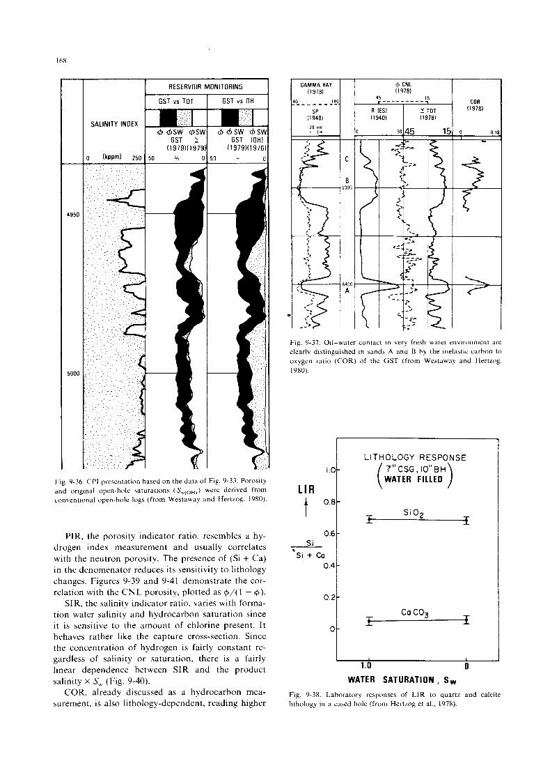
I6X
1.0-
L I R
f O.*-
0.6 Si
Si + Ca .
0.4
0.2-
4950
5000
LITHOLOGY RESPONSE 7 " C S G , IO"BH
WATER FILLED
f Si 0 2
f -
-
I RESERVOIR M O N I T O R I N G 1
SALINITY INOEX
I d, chsw chsw GST (OH)
10 " 979)11976)~ ',- 0
Fig. 9-36. CPI presentation based on the data of Fig. 9-33. Porosity and original open-hole saturations (S, , , , , , ) were derived from conventional open-hole logs (from Westaway and Hertzog, 1980).
PIR, the porosity indicator ratio, resembles a hy- drogen index measurement and usually correlates with the neutron porosity. The presence of (Si + Ca) in the denomenator reduces its sensitivity to lithology changes. Figures 9-39 and 9-41 demonstrate the cor- relation with the CNL porosity, plotted as +/( 1 - +).
SIR, the salinity indicator ratio. varies with forma- tion water salinity and hydrocarbon saturation since i t is sensitive to the amount of chlorine present. I t behaves rather like the capture cross-section. Since the concentration of hydrogen is fairly constant re- gardless of salinity or saturation, there is a fairly linear dependence between SIR and the product salinity x S, (Fig. 9-40).
COR, already discussed as a hydrocarbon mea- surement, is also lithology-dependent, reading higher
GAMMA RAY 11978)
SP (19401 I 20 rnV - I I*
COR (1978)
w
f
Fig. 9-37. Oil-water contact in very fresh water environment are clearly distinguished in sands A and B by the inelastic carbon to oxygen ratio (COR) of the GST (from Westaway and Hertzog. 1980).
I 1 I I 1.0 0
WATER S A T U R A T I O N , S w
Fig. 9-38. Laboratory responses of LIR to quartz and calcite lithology in a cased hole (from Hertzog et al.. 1978).
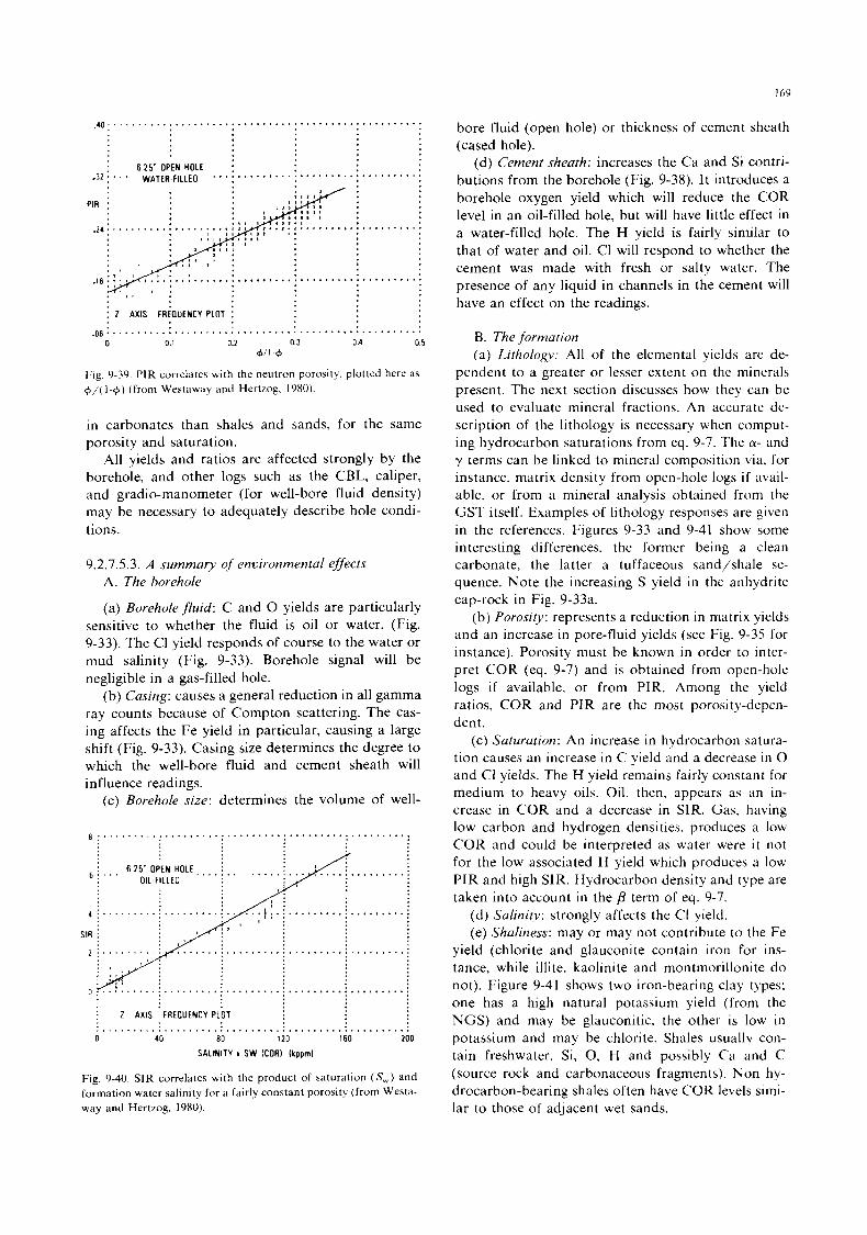
169
...................................................
: 6 2 5 " OPEN HOLE : . . . WATER ..................................
. , I
i 2 AXIS F R h J E N C Y PLOT
.08 ................................................... 0 0.1 0.2 0.3 04 0.5
611 6
Fig. 9-39, PIR correlates with the neutron porosity. plotted here as +/( 1-4) (from Westaway and Hertzog. 1980).
in carbonates than shales and sands, for the same porosity and saturation.
All yields and ratios are affected strongly by the borehole, and other logs such as the CBL, caliper, and gradio-manometer (for well-bore fluid density) may be necessary to adequately describe hole condi- tions.
9.2.7.5.3. A summary of environmental effects A. The borehole
(a) Boreholefluid: C and 0 yields are particularly sensitive to whether the fluid is oil or water. (Fig. 9-33). The C1 yield responds of course to the water or mud salinity (Fig. 9-33). Borehole signal will be negligible in a gas-filled hole.
(b) Casing: causes a general reduction in all gamma ray counts because of Compton scattering. The cas- ing affects the Fe yield in particular, causing a large shift (Fig. 9-33). Casing size determines the degree to which the well-bore fluid and cement sheath will influence readings.
(c) Borehole size: determines the volume of well-
8 : " " ..............................................
E , . . . :
4 i I . . : .
6 25" OPEN HOLE 011 FILLED
.IP . Sl"
2
0
. . . . . . . . . . . . . . .
................................................ : 2 AXIS FAEOUENCY PLOT . . ................................................. 0 40 80 120 160 200
S A L N I T Y I SW (COR) (kppm)
Fig. 9-40. SIR correlates with the product of saturation ( S , ) and formation water salinity for a fairly constant porosity (from Westa- way and Hertzog. 1980).
bore fluid (open hole) or thickness of cement sheath (cased hole).
(d) Cement sheath: increases the Ca and Si contri- butions from the borehole (Fig. 9-38). It introduces a borehole oxygen yield which will reduce the COR level in an oil-filled hole, but will have little effect in a water-filled hole. The H yield is fairly similar to that of water and oil. C1 will respond to whether the cement was made with fresh or salty water. The presence of any liquid in channels in the cement will have an effect on the readings.
B. The formation (a) Lithology: All of the elemental yields are de-
pendent to a greater or lesser extent on the minerals present. The next section discusses how they can be used to evaluate mineral fractions. An accurate de- scription of the lithology is necessary when coniput- ing hydrocarbon saturations from eq. 9-7. The a- and y terms can be linked to mineral composition via, for instance, matrix density from open-hole logs i f avail- able, or from a mineral analysis obtained from the GST itself. Examples of lithology responses are given in the references. Figures 9-33 and 9-41 show some interesting differences, the former being a clean carbonate, the latter a tuffaceous sand/shale se- quence. Note the increasing S yield in the anhydrite cap-rock in Fig. 9-33a.
(b) Porosity: represents a reduction in matrix yields and an increase in pore-fluid yields (see Fig. 9-35 for instance). Porosity must be known in order to inter- pret COR (eq. 9-7) and is obtained from open-hole logs i f available. or from PIR. Among the yield ratios, COR and PIR are the most porosity-depen- dent.
(c) Saturution: An increase in hydrocarbon satura- tion causes an increase in C yield and a decrease in 0 and CI yields. The H yield remains fairly constant for medium to heavy oils. Oil, then, appears as an in- crease in COR and a decrease in SIR. Gas, having low carbon and hydrogen densities. produces a low COR and could be interpreted as water were i t not for the low associated H yield which produces a low PIR and high SIR. Hydrocarbon density and type are taken into account in the p term of eq. 9-7.
(d) Salinity: strongly affects the CI yield. (e) Shaliness: may or may not contribute to the Fe
yield (chlorite and glauconite contain iron for ins- tance, while illite, kaolinite and montmorillonite do not). Figure 9-41 shows two iron-bearing clay types; one has a high natural potassium yield (from the NGS) and may be glauconitic. the other is low in potassium and may be chlorite. Shales usually con- tain freshwater, Si, 0, H and possibly Ca and C (source rock and carbonaceous fragments). Non hy- drocarbon-bearing shales often have COR levels simi- lar to those of adjacent wet sands.
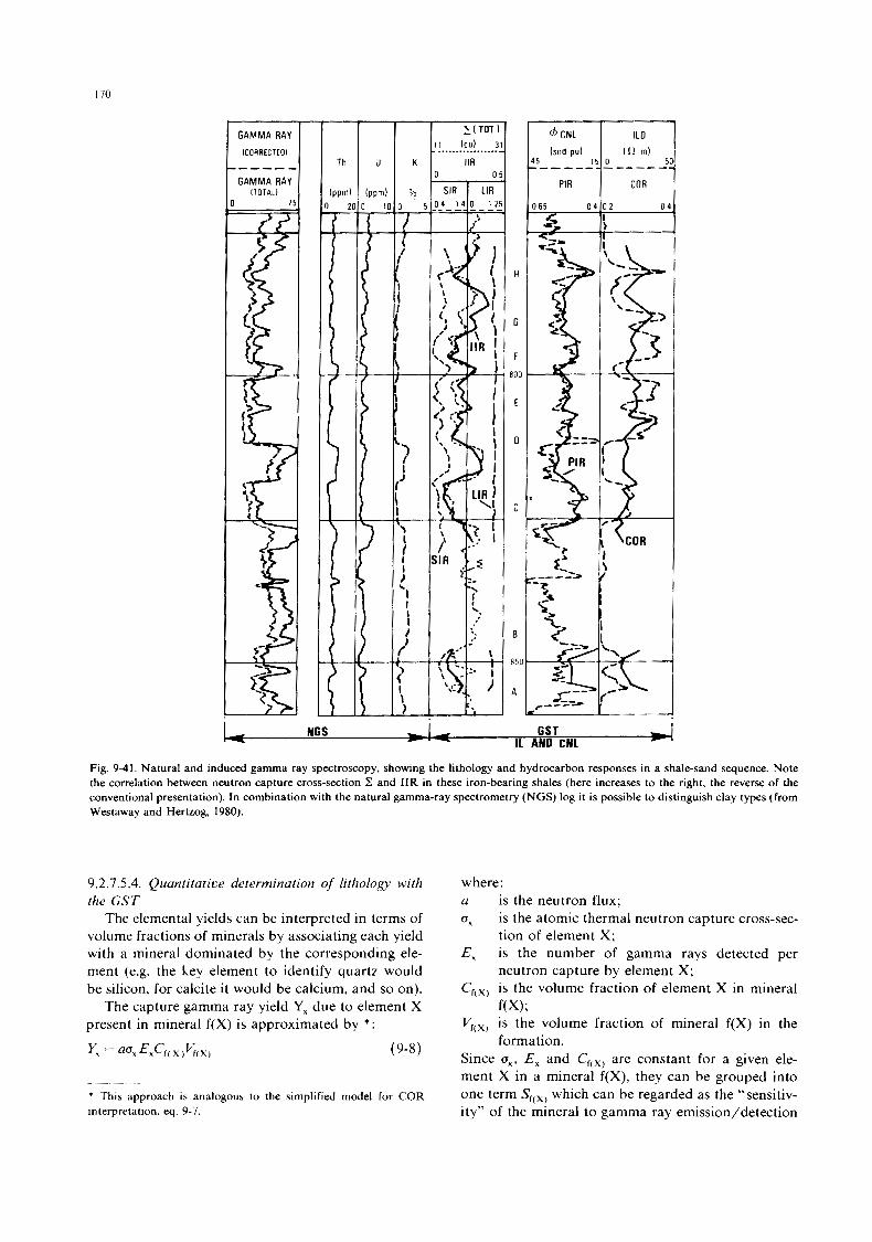
170
H
G
F
R O O
E
0
C
E
8 ’
P
GST 4 I1 AND CNL NGS
Fig. 9-41. Natural and induced gamma ray spectroscopy, showing the lithology and hydrocarbon responses in a shale-sand sequence. Note the correlation between neutron capture cross-section Z and IIR in these iron-bearing shales (here increases to the right, the reverse of the conventional presentation). In combination with the natural gamma-ray spectrometry (NGS) log it is possible to distinguish clay types (from Westaway and Hertzog, 1980).
9.2.1.5.4. Quantitative determination of lithology with the GST
The elemental yields can be interpreted in terms of volume fractions of minerals by associating each yield with a mineral dominated by the corresponding ele- ment (e.g. the key element to identify quartz would be silicon, for calcite it would be calcium, and so on).
The capture gamma ray yield Y , due to element X present in mineral f(X) is approximated by *:
y x = U % E x C f ( X Y N X ) (9-8)
~ -~ ~~-
* This approach is analogous to the simplified model for COR interpretation, eq. 9-7.
where: a is the neutron flux; u, is the atomic thermal neutron capture cross-sec-
tion of element X; E , is the number of gamma rays detected per
neutron capture by element X; Cr0, is the volume fraction of element X in mineral
V,,,, is the volume fraction of mineral f(X) in the
Since ux, E , and C,,,, are constant for a given ele- ment X in a mineral f(X), they can be grouped into one term Sf(x! which can be regarded as the “sensitiv- ity” of the mineral to gamma ray emission/detection
f(X);
formation.
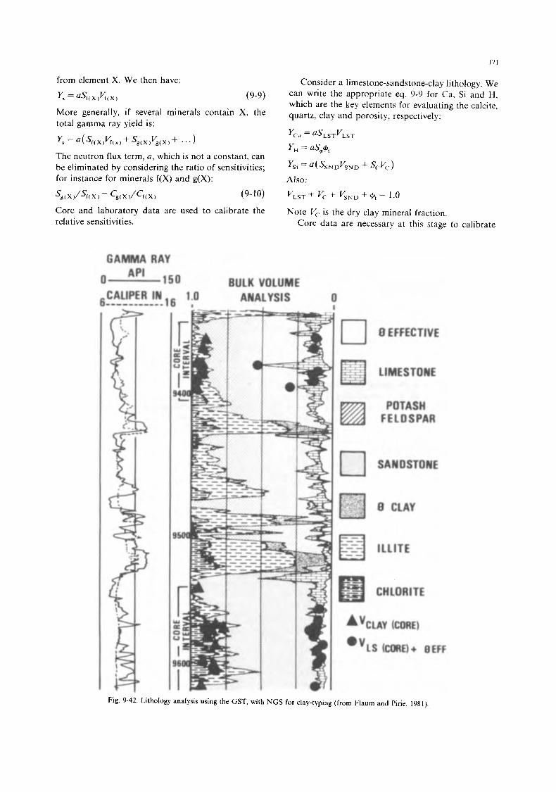
171
from element X. We then have: Consider a limestone-sandstone-clay lithology. We can write the appropriate eq. 9-9 for Ca, Si and H, which are the key elements for evaluating the calcite, quartz, clay and porosity, respectively:
(9-9)
More generally, if several minerals contain x , the y, = G(X)Vf(X)
total gamma ray yield is:
y, = a(sf(X)Vf(,) + sg(x)Vg(x) + . . The neutron flux term, a, which is not a constant, can be eliminated by considering the ratio of sensitivities; for instance for minerals f(X) and g(X):
'Si = a ( S ~ ~ ~ V ~ ~ ~ + scVc) Also:
sg(x)/sf(x) = Cg(X)/Cf(X) (9-10) VLsT + V, + VsND + 9, = 1 .O
Core and laboratory data are used to calibrate the relative sensitivities.
Note Vc is the dry clay mineral fraction. Core data are necessary at this stage to calibrate
G A M M A RAY
0 1 5 0 BULK VOLUME 6----------- CALIPER IN 1 6 1.0 , ANALYSIS 0
1
rl 8 EFFECTIVE
LIMESTONE
POTASH FELDSPAR
SANDSTONE
ILL ITE
&LAY (CORE)
OVLs (CORE)+ 8EFF
Fig. 9-42. Lithology analysis using the GST, with NGS for clay-typing (from Flaum and Pirie. 1981)
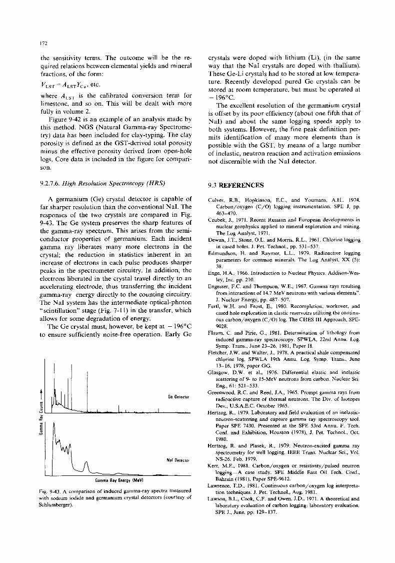
172
the sensitivity terms. The outcome will be the re- quired relations between elemental yields and mineral fractions, of the form:
VLST = ALSTYCa, etc. where ALST is the calibrated conversion term for limestone, and so on. This will be dealt with more fully in volume 2.
Figure 9-42 is an example of an analysis made by this method. NGS (Natural Gamma-ray Spectrome- try) data has been included for clay-typing. The clay porosity is defined as the GST-derived total porosity minus the effective porosity derived from open-hole logs. Core data is included in the figure for compari- son.
9.2.7.6. High Resolution Spectroscopy (HRS)
A germanium (Ge) crystal detector is capable of far sharper resolution than the conventional NaI. The responses of the two crystals are compared in Fig. 9-43. The Ge system preserves the sharp features of the gamma-ray spectrum. This arises from the semi- conductor properties of germanium. Each incident gamma ray liberates many more electrons in the crystal; the reduction in statistics inherent in an increase of electrons in each pulse produces sharper peaks in the spectrometer circuitry. In addition, the electrons liberated in the crystal travel directly to an accelerating electrode, thus transferring the incident gamma-ray energy directly to the counting circuitry. The NaI system has the intermediate optical-photon “scintillation” stage (Fig. 7-1 1) in the transfer, which allows for some degradation of energy.
The Ge crystal must, however, be kept at - 196°C to ensure sufficiently noise-free operation. Early Ge
Gamma Ray Energy (MeV)
Fig. 9-43. A comparison of induced gamma-ray spectra measured with sodium iodide and germanium crystal detectors (courtesy of Schlumberger).
crystals were doped with lithium (Li), (in the same way that the NaI crystals are doped with thallium). These Ge-,Li crystals had to be stored at low tempera- ture. Recently developed pured Ge crystals can be stored at room temperature, but must be operated at
The excellent resolution of the germanium crystal is offset by its poor efficiency (about one fifth that of NaI) and about the same logging speeds apply to both systems. However, the fine peak definition per- mits identification of many more elements than is possible with the GST, by means of a large number of inelastic, neutron reaction and activation emissions not discernible with the NaI detector.
- 196°C.
9.3 REFERENCES
Culver, R.B., Hopkinson, E.C., and Youmans, A.H., 1974. Carbon/oxygen (C/O) logging instrumentation. SPE J, pp. 463-470.
Czubek, J., 1971. Recent Russian and European developments in nuclear geophysics applied to mineral exploration and mining. The Log Analyst, 1971.
Dewan, J.T., Stone, O.L. and Morris, R.L., 1961. Chlorine logging in cased holes. J. Pet. Technol., pp. 531-537.
Edmundson, H. and Raymer, L.L., 1979. Radioactive logging parameters for common minerals. The Log Analyst, XX ( 5 ) : 38.
Enge, H.A., 1966. Introduction to Nuclear Physics. Addison-Wes- ley, Inc. pp. 210.
Engesser, F.C. and Thompson, W.E., 1967. Gamma rays resulting from interactions of 14.7 MeV neutrons with various elements”. J. Nuclear Energy, pp. 487-507.
Fertl, W.H. and Frost, E., 1980. Recompletion, workover, and cased hole exploration in clastic reservoirs utilizing the continu- ous carbon/oxygen (C/O) log. The CHES Il l Approach, SPE- 9028.
Flaum, C. and Pirie, G., 1981. Determination of lithology from induced gamma-ray spectroscopy. SPWLA, 22nd Annu. Log. Symp. Trans., June 23-26, 1981, Paper H.
Fletcher, J.W. and Walter, J., 1978. A practical shale compensated chlorine log. SPWLA 19th Annu. Log. Symp. Trans., June 13-16, 1978, paper GG.
Glasgow, D.W. et al., 1976. Differential elastic and inelastic scattering of 9- to 15-MeV neutrons from carbon. Nuclear Sci. Eng., 61: 521-533.
Greenwood, R.C. and Reed, J.A., 1965. Prompt gamma rays from radioactive capture of thermal neutrons. The Div. of Isotopes Dev., U.S.A.E.C. October 1965.
Hertzog, R., 1979. Laboratory and field evaluation of an inelastic- neutron-scattering and capture gamma ray spectroscopy tool. Paper SPE 7430. Presented at the SPE 53rd Annu. F. Tech. Conf. and Exhibition, Houston (1978), J. Pet. Technol., Oct. 1980.
Hertzog, R. and Plasek, R., 1979. Neutron-excited gamma ray spectrometry for well logging. IEEE Trans. Nuclear Sci., Vol. NS-26. Feb. 1979.
Kerr, M.E., 1981. Carbon/oxygen or resistivity/pulsed neutron logging-A case study. SPE Middle East Oil Tech. Conf., Bahrain (1981), Paper SPE-9612.
Lawrence, T.D., 198 1. Continuous carbon/oxygen log interpreta- tion techniques. J. Pet. Technol., Aug. 1981.
Lawson, B.L., Cook, C.F. and Owen, J.D., 1971. A theoretical and laboratory evaluation of carbon logging: laboratory evaluation. SPE J., June, pp. 129-137.
I73
Lock, G.A. and Hoyer, W.A., 1974. Carbon/oxygen (C/O) log: use and interpretation. J. Pet. Technol., Sept., pp. 1044-1054.
McKinlay. P.F. and Tanner, H.L., 1975. The shale compensated chlorine log. J . Pet. Technol., Feb., pp. 164-170.
Moran, H.H. and Tittman, J., 1970. Analysis of gamma-ray energy spectrum for constituent identification. U.S. Patent 3,521,064 (July 21st 1970).
Oliver. D.W. et al., I98 I . Continuous carbon/oxygen logging-in- strumentation, interpretive concepts and field applications. SPWLA, 22nd Ann. Log. Symp. Trans., Paper TT.
Rabson, W.R.. 1969. Chlorine detection by the spectral log. Pet. Eng., Mar. 1969, B102-llI.
Ready, R., Arnold, J. and Trombka, J., 1973. Expected gamma-ray emissions spectra from the lunar surface as a function of chemical composition. Gold Space Flight Center, Publ. No. X-641-73-68.
Reike, H. et al., 1980. Successful application of carbon/oxygen logging to coal bed exploration. SPE 9464.
Schultz, W.E. and Smith, H.D., Jr., 1973. Laboratory and field evaluation of a carbon/oxygen well logging system. SPE-4638.
Smith, H.D. and Schultz, W.E.. 1974. Field experience in determin-
ing oil saturations from continuous C/O and Ca/Si logs independent of salinity and shaliness. The Log Analyst. Nov- Dec. 1974, pp. 9-18.
Stroud, S.G. and Schaller, H.E., 1960. New radiation log for the determination of reservoir salinity. J. Pet. Technol.. Feb.. pp. 37-41.
Tittman, J. and Nelligan, W.B., 1960. Laboratory studles of a pulsed neutron-source technique in well logging. SPE AIME, Trans. 219: 375-378.
Waddell, C. and Wilson, J.C., 1960. Chlorinity and porosity de- termination in cased and open holes by nuclear logs. SPE of AIME, Paper 1456-G, Beaumont. Texas, Mar 8, 1960.
Westaway, P. and Hertzog, R., 1980. The gamma spectrometer tool: inelastic and capture gamma-ray spectroscopy for re- servoir analysis. Paper SPE-9461.
Westaway, P., Wittmann, M. and Rochette, P., 1979. Applications of nuclear techniques to reservoir monitoring. Proc. SPE Mid- dle East Tech. Conf., Bahrain, Paper SPE-7776.
Youngblood, W., 1980. The application of pulsed-neutron decay time logs to monitoring water floods with changing salinity. J . Pet. Technol., 32/6.

This Page Intentionally Left Blank
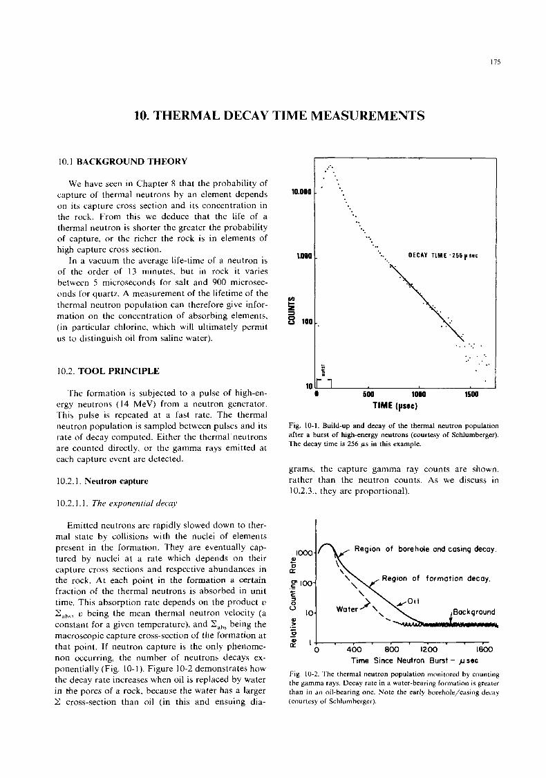
175
10. THERMAL DECAY TIME MEASUREMENTS
10.1 BACKGROUND THEORY
We have seen in Chapter 8 that the probability of capture of thermal neutrons by an element depends on its capture cross section and its concentration in the rock. From this we deduce that the life of a thermal neutron is shorter the greater the probability of capture, or the richer the rock is in elements of high capture cross section.
In a vacuum the average life-time of a neutron is of the order of 13 minutes, but in rock it varies between 5 microseconds for salt and 900 microsec- onds for quartz. A measurement of the lifetime of the thermal neutron population can therefore give infor- mation on the concentration of absorbing elements, (in particular chlorine, which will ultimately permit us to distinguish oil from saline water).
10.2. TOOL PRINCIPLE
The formation is subjected to a pulse of high-en- ergy neutrons (14 MeV) from a neutron generator. This pulse is repeated at a fast rate. The thermal neutron population is sampled between pulses and its rate of decay computed. Either the thermal neutrons are counted directly, or the gamma rays emitted at each capture event are detected.
10.2.1. Neutron capture
10.2.1.1. The exponentid decay
Emitted neutrons are rapidly slowed down to ther- mal state by collisions with the nuclei of elements present in the formation. They are eventually cap- tured by nuclei at a rate which depends on their capture cross sections and respective abundances in the rock. At each point in the formation a certain fraction of the thermal neutrons is absorbed in unit time. This absorption rate depends on the product u Zc,h,, u being the mean thermal neutron velocity (a constant for a given temperature), and Zaha being the macroscopic capture cross-section of the formation at that point. If neutron capture is the only phenome- non occurring, the number of neutrons decays ex- ponentially (Fig. 10-1). Figure 10-2 demonstrates how the decay rate increases when oil is replaced by water in the pores of a rock, because the water has a larger Z cross-section than oil (in this and ensuing dia-
10.000
1.000
r 00 100
z 3
10
.. . . . .
DECAY TIME - 2 5 6 p sec
. . . . .
r c.3 c
1 7
500 1000 1500
TIME (psec)
Fig. 10-1. Build-up and decay of the thermal neutron population after a burst of high-energy neutrons (courtesy of Schlumberger). The decay time is 256 ps in this example.
grams, the capture gamma ray counts are shown, rather than the neutron counts. As we discuss in 10.2.3., they are proportional).
Region of borehole and casing decoy. IOOO- aJ 0 [L
c
Region of formotion decoy. 100- -
c c 1 0 0
aJ > 10-
._
Region of formotion decoy.
c c 1 0 0
aJ > ._ Z J -
$ 1 0 400 800 1200 I800
Time Since Neutron Burst - y s r c
Fig. 10-2. The thermal neutron population monitored by counting the gamma rays. Decay rate in a water-bearing formation is greater than in an oil-bearing one. Note the early borehole/casing decay (courtesy of Schlumberger).
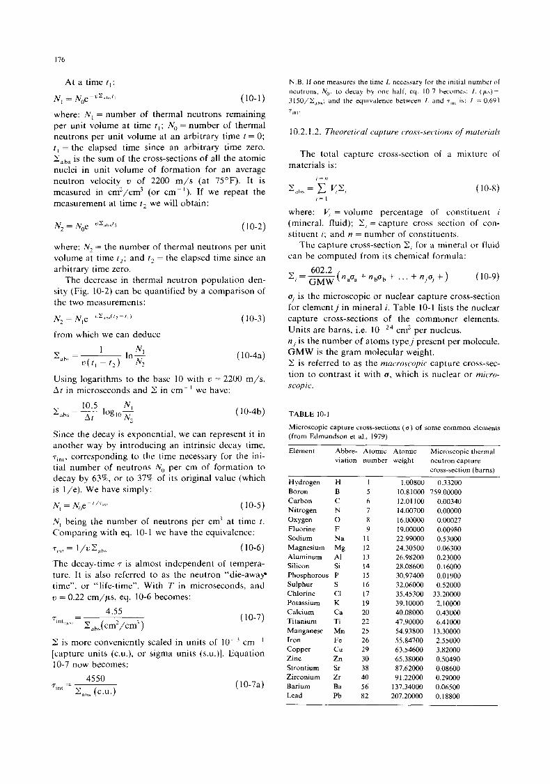
I76
At a time t , :
N, = Noe-"xah.." (10-1)
where: N, = number of thermal neutrons remaining per unit volume at time t , ; No = number of thermal neutrons per unit volume at an arbitrary time t = 0; t , = the elapsed time since an arbitrary time zero. Zabs is the sum of the cross-sections of all the atomic nuclei in unit volume of formation for an average neutron velocity u of 2200 m/s (at 75°F). It is measured in cm2/cm3 (or cm-I). If we repeat the measurement at time t , we will obtain:
( 10-2)
where: N7 = the number of thermal neutrons per unit volume at time t,; and t , = the elapsed time since an arbitrary time zero.
The decrease in thermal neutron population den- sity (Fig. 10-2) can be quantified by a comparison of the two measurements:
from which we can deduce
( 10-4a)
Using logarithms to the base 10 with u = 2200 m/s, At in microseconds and Z in cm-l we have:
( 10-4b)
Since the decay is exponential, we can represent i t in another way by introducing an intrinsic decay time, T,"~, corresponding to the time necessary for the ini- tial number of neutrons No per cm of formation to decay by 63%, or to 37% of its original value (which is l/e). We have simply:
N, = N,,e- l/Tm (10-5)
N , being the number of neutrons per cm' at time t . Comparing with eq. 10-1 we have the equivalence:
7 , n t = l/UZ'lh, ( 10-6)
The decay-time r is almost independent of tempera- ture. I t is also referred to as the neutron "die-away time", or "life-time". With T in microseconds, and u = 0.22 cm/ps, eq. 10-6 becomes:
4.55 -
Iilh5( cm2/cm3 ) r l n , ,p \ , - ( 10-7)
2: is more conveniently scaled in units of lo-' cm- ' [capture units (c.u.), or sigma units (s.u.)]. Equation 10-7 now becomes:
( 10-7a)
N.B. I f one measures the time L necessary for the initial number of neutrons, N,, , to decay by one half, eq. 10-7 hecomes: L ( p s ) = 3150/2,,,; and the equivalence between L and T,,,, is: L. = 0.693 7,"l.
10.2.1.2. Theoreticul cupture cros.s-section.s of niuteriuls
The total capture materials is:
, = n
C a b \ = c v, I = I
where: V; = volume
cross-section of a mixture of
( 10-8)
percentage of constituent i (mineral, fluid); 2, = capture cross section of con- stituent i; and n = number of constituents.
The capture cross-section C, for a mineral or fluid can be computed from its chemical formula:
602.2 GMW z,=- (n ,a ,+nbu,+ . . . + n,o, + 1 ( 10-9)
a, is the microscopic or nuclear capture cross-section for elementj in mineral i. Table 10-1 lists the nuclear capture cross-sections of the commoner elements. Units are barns, i.e. n, is the number of atoms typej present per molecule. GMW is the gram molecular weight. I: is referred to as the macroscopic capture cross-sec- tion to contrast i t with u, which is nuclear or micro- scopic.
cm2 per nucleus.
TABLE 10-1
Microscopic capture cross-sections ( u ) of some common elements (from Edmundson et al., 1979)
~
Element Abbre- Atomic Atomic Microscopic thermal
cross-section (barns) viation number weight neutron capture
Hydrogen Boron Carbon Nitrogen Oxygen Fluorine Sodium Magnesium Aluminum Silicon Phosphorous Sulphur Chlorine Potassium Calcium Titanium Manganese Iron Copper Zinc Strontium Zirconium Barium Lead
H 1 B 5 C 6 N 7 0 8 F 9 Na 11 Mg 12 A1 13 Si 14 P 15 S 16 c1 17 K 19 Ca 20 Ti 22 Mn 25 Fe 26 Cu 29 Zn 30 Sr 38 Zr 40 Ba 56 Pb 82
1.00800 10.81000 12.01 100 14.00700 16.00000 19.00000 22.99000 24.30500 26.98200 28.08600 30.97400 32.06000 35.45300 39.10000 40.08000 47.90000 54.93800 55.84700 63.54600 65.38000 87.62000 9 1.22000
137.34000 207.2oooO
0.3 3 200 759.00000
0.00340 0.00000 0.00027 0.00980 0.53000 0.06300 0.23000 0.16000 0.0 1900 0.5 2000
33.20000 2.10000 0.43000 6.4 1000
13.30000 2.55000 3.82000 0.50490 0.08600 0.29000 0.06500 0.18800
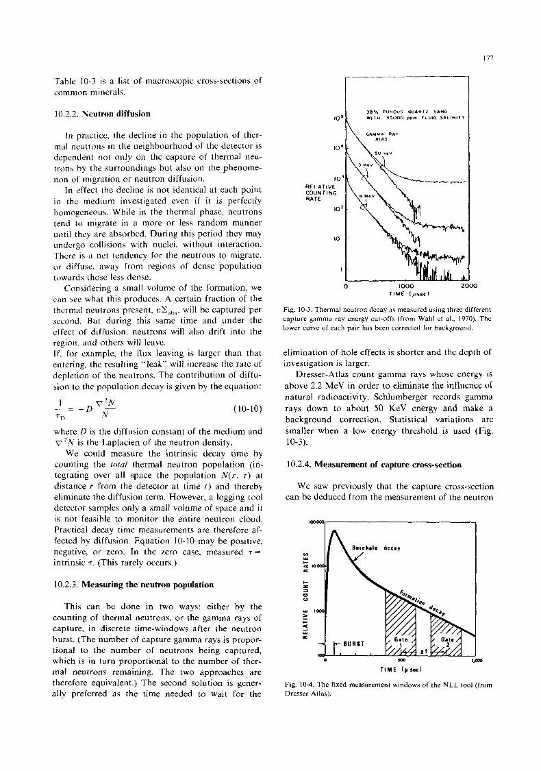
177
Table 10-3 is a list of macroscopic cross-sections of common minerals.
10.2.2. Neutron diffusion
I n practice, the decline in the population of ther- mal neutrons in the neighbourhood of the detector is dependent not only on the capture of thermal neu- trons by the surroundings but also on the phenome- non o f migration or neutron diffusion.
In effect the decline is not identical at each point in the medium investigated even if i t is perfectly homogeneous. While in the thermal phase, neutrons tend to migrate in a more or less random manner until they are absorbed. During this period they may undergo collisions with nuclei, without interaction. There is a net tendency for the neutrons to migrate, or diffuse, away from regions of dense population towards those less dense.
Considering a small volume of the formation, we can see what this produces. A certain fraction of the thermal neutrons present, 0 2 , ~ ~ . will be captured per second. But during this same time and under the effect of diffusion, neutrons will also drift into the region, and others will leave. I f , for example, the flux leaving is larger than that entering, the resulting “leak” will increase the rate of depletion of the neutrons. The contribution of diffu- sion to the population decay is given by the equation:
v ’ N - -D- 1 _ - 711 N
(10-10)
where D is the diffusion constant of the medium and v ’ N is the Laplacien of the neutron density.
We could measure the intrinsic decay time by counting the total thermal neutron population (in- tegrating over all space the population N ( r , t ) at distance r from the detector at time t ) and thereby eliminate the diffusion term. However, a logging tool detector samples only a small volume of space and i t is not feasible to monitor the entire neutron cloud. Practical decay time measurements are therefore af- fected by diffusion. Equation 10-10 may be positive, negative, or zero. In the zero case, measured r =
intrinsic r . (This rarely occurs.)
10.2.3. Measuring the neutron population
This can be done in two ways: either by the counting of thermal neutrons, or the gamma rays of capture, in discrete time-windows after the neutron burst. (The number of capture gamma rays is propor- tional to the number of neutrons being captured, which is in turn proportional to the number of ther- mal neutrons remaining. The two approaches are therefore equivalent.) The second solution is gener- ally preferred as the time needed to wait for the
30-1. POROUS OUARfZ SAND W t l H 95000 DDm f L U l 0 S A L I N I I V
G4MH4 A 4 f h B l P S
10’
0 I000 2000 TIME I p 5 e c )
Fig. 10-3. Thermal neutron decay as measured using three different capture gamma ray energy cut-offs (from Wahl et al., 1970). The lower curve of each pair has been corrected for background.
elimination of hole effects is shorter and the depth of investigation is larger.
Dresser-Atlas count gamma rays whose energy is above 2.2 MeV in order to eliminate the influence of natural radioactivity. Schlumberger records gamma rays down to about 50 KeV energy and make a background correction. Statistical variations are smaller when a low energy threshold is used (Fig. 10-3).
10.2.4. Measurement of capture cross-section
We saw previously that the capture cross-section can be deduced from the measurement of the neutron
.. ...
TIME ( p s e c )
Fig. 10-4. The fixed measurement windows of the NLL tool (from Dresser Atlas).
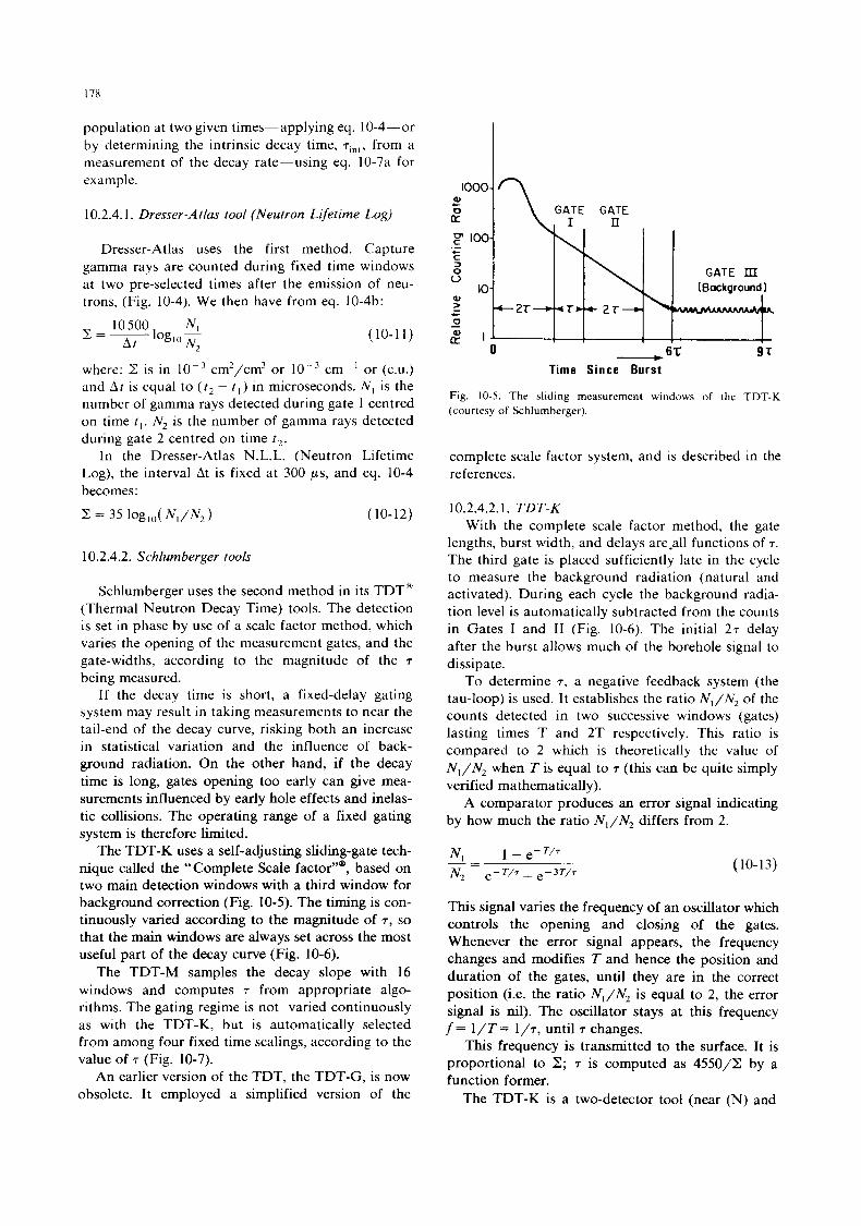
178
population at two given times-applying eq. 10-4-or by determining the intrinsic decay time, r,,,,, from a measurement of the decay rate-using eq. 10-7a for example.
10.2.4.1. Dresser-Atlas tool (Neutron Lifetime Log)
Dresser-Atlas uses the first method. Capture gamma rays are counted during fixed time windows at two pre-selected times after the emission of neu- trons, (Fig. 10-4). We then have from eq. 10-4b:
(10-1 1 )
where: Z is in l o p 3 cm2/cm3 or lo-’ c m p ’ or (c.u.) and A t is equal to ( t , - t l ) in microseconds. N, is the number of gamma rays detected during gate 1 centred o n time t , . N2 is the number of gamma rays detected during gate 2 centred on time t,.
In the Dresser-Atlas N.L.L. (Neutron Lifetime Log), the interval At is fixed at 300 ps, and eq. 10-4 becomes: 2 = 35 log,o(N,/N2) (10-12)
10.2.4.2. Schlumberger tools
Schlumberger uses the second method in its TDTa (Thermal Neutron Decay Time) tools. The detection is set in phase by use of a scale factor method, which varies the opening of the measurement gates, and the gate-widths, according to the magnitude of the r
being measured. If the decay time is short, a fixed-delay gating
system may result in taking measurements to near the tail-end of the decay curve, risking both an increase in statistical variation and the influence of back- ground radiation. On the other hand, if the decay time is long, gates opening too early can give mea- surements influenced by early hole effects and inelas- tic collisions. The operating range of a fixed gating system is therefore limited.
The TDT-K uses a self-adjusting sliding-gate tech- nique called the “Complete Scale factor”@, based on two main detection windows with a third window for background correction (Fig. 10-5). The timing is con- tinuously varied according to the magnitude of T, so that the main windows are always set across the most useful part of the decay curve (Fig. 10-6).
The TDT-M samples the decay slope with 16 windows and computes r from appropriate algo- rithms. The gating regime is not varied continuously as with the TDT-K, but is automatically selected from among four fixed time scalings, according to the value of 7 (Fig. 10-7).
An earlier version of the TDT, the TDT-G, is now obsolete. It employed a simplified version of the
1000 al
0 c
rK
loo .- c c 3 0 u al I
10
c 0 -
7 GATE GATE
B I 0
II
GATE IlI (Background)
Time Since Burst
Fig. 10-5. The sliding measurement windows o f the TDT-K (courtesy of Schlumberger).
complete scale factor system, and is described in the references.
10.2.4.2.1. TDT-K With the complete scale factor method, the gate
lengths, burst width, and delays are-all functions of r .
The third gate is placed sufficiently late in the cycle to measure the background radiation (natural and activated). During each cycle the background radia- tion level is automatically subtracted from the counts in Gates I and I1 (Fig. 10-6). The initial 27 delay after the burst allows much of the borehole signal to dissipate.
To determine r , a negative feedback system (the tau-loop) is used. It establishes the ratio N,/N, of the counts detected in two successive windows (gates) lasting times T and 2T respectively. This ratio is compared to 2 which is theoretically the value of N 1 / N z when T is equal to T ( th s can be quite simply verified mathematically).
A comparator produces an error signal indicating by how much the ratio N 1 / N 2 differs from 2.
(10-13)
This signal varies the frequency of an oscillator which controls the opening and closing of the gates. Whenever the error signal appears, the frequency changes and modifies T and hence the position and duration of the gates, until they are in the correct position (i.e. the ratio N , / N , is equal to 2, the error signal is nil). The oscillator stays at this frequency f = 1 / T = I / T , until T changes.
This frequency is transmitted to the surface. It is proportional to 2; 7 is computed as 4550/2 by a function former.
The TDT-K is a two-detector tool (near (N) and
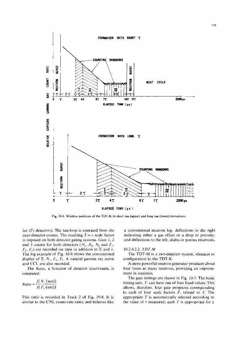
1 1 179
FORMATION WITH SHORT Z
ELAPSED TIME ( ps
FORMATION WITH LONG
O 3T 4-c 6T 7f 2000 ps
ELAPSEd TIME I ps
Fig. 10-6. Window positions of the TDT-K in short tau (upper) and long tau (lower) formations.
far (F) detectors). The tau-loop is operated from the near-detector counts. The resulting T = T scale factor is imposed on both detector gating systems. Gate 1, 2 and 3 counts for both detectors ( N , , N , , N3 and F, , F,, F 7 ) are recorded on tape in addition to Z and T. The log example of Fig. 10-8 shows the conventional display of Z, N , , F , , F3. A natural gamma ray curve and CCL are also recorded.
The Ratio, a function of detector count-rates, is computed:
This ratio is recorded in Track 2 of Fig. 10-8. It is similar to the CNL count-rate ratio, and behaves like
a conventional neutron log: deflections to the right indicating either a gas effect or a drop in porosity, and deflections to the left, shales or porous reservoirs.
10.2.4.2.2. TDT-M The TDT-M is a two-detector system, identical in
configuration to the TDT-K. A more powerful neutron generator produces about
four times as many neutrons, providing an improve- ment in statistics.
The gate timings are shown in Fig. 10-7. The basic timing unit, T, can have one of four fixed values. This allows, therefore, four gate programs corresponding to each of four scale factors F, related to T. The appropriate T is automatically selected according to the value of T measured; each T is appropriate for a
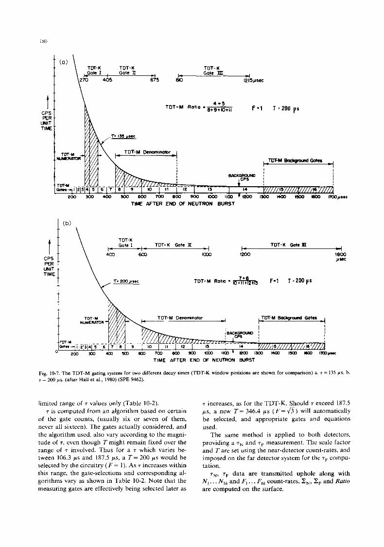
TDT-K TDT- K
k Gote lE 4 270 405 675 810 1215r~c
t \ t t \
4 +5 8+ 9t K)+I I F - t T =200 vs TDT-M Ratio I I
CPS PER
U(IT TIME
TIME AFTER END OF NEUTRON BURST
(b)
TOT-K TOT-K Gate SI TOT-K GoteI
4 600 1030 I200 I800
Ira
7- 200pr.c TOT-M Ratm = B*B F-1 T.200 V S
t CPS PER UNIT TIME
1 TOT-M I.. TOT-M Ocnormnator NUMERATOR = I
TIME AFTER EN0 OF NEUTRON BURST
Fig. 10-7. The TDT-M gating system for two different decay times (TDT-K window positions are shown for comparison) a. T = 135 p s . b. T = 200 p s . (after Hall et al., 1980) (SPE 9462).
limited range of T values only (Table 10-2). 7 is computed from an algorithm based on certain
of the gate counts, (usually six or seven of them, never all sixteen). The gates actually considered, and the algorithm used, also vary according to the magni- tude of 7, even though T might remain fixed over the range of 7 involved. Thus for a T which varies be- tween 106.3 p s and 187.5 p s , a T = 200 p s would be selected by the circuitry ( F = 1). As 7 increases within this range, the gate-selections and corresponding al- gorithms vary as shown in Table 10-2. Note that the measuring gates are effectively being selected later as
7 increases, as for the TDT-K. Should T exceed 187.5 p s , a new T = 346.4 ps ( F = 0) will automatically be selected, and appropriate gates and equations used.
The same method is applied to both detectors, providing a T~ and T~ measurement. The scale factor and Tare set using the near-detector count-rates, and imposed on the far detector system for the 7F compu- tation.
T ~ , rF data are transmitted uphole along with N , . . . N , , and Fl. . . F,, count-rates. Z,, Z, and Ratio are computed on the surface.
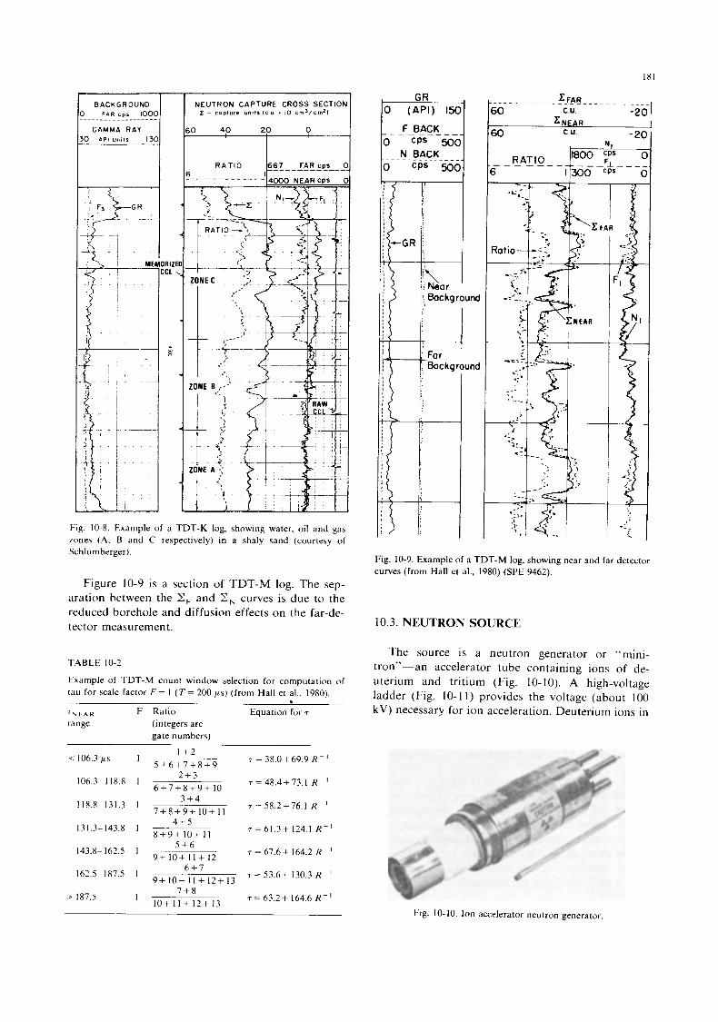
BACKGROUND F A R c p i 1000
GAMMA R A Y
1 Mf RlZl CL
6
NEUTRON CAPTURE CROSS SECTlOl z - C O P I U ~ C u n t ~ s ( c u = 10 cm’/cm2)
i0 40 20 0
Fig. 10-8. Example of a TDT-K log, showing water, oil and gas zones (A, B and C respectively) in a shaly sand (courtesy of Schlumberger).
Figure 10-9 is a section of TDT-M log. The sep- aration between the Z, and Z, curves is due to the reduced borehole and diffusion effects on the far-de- tector measurement.
TABLE 10-2
Example o f TDT-M count window selection for computation of tau for scale factor F = 1 ( T = 200 ps) (from Hall et al., 1980).
T~~~~ F Ratio Equation for T range (integers are
. gate numbers)
~
1 + 2 5 + 6 + 7 + 8 + 9
2 + 3 6 + 7 + 8 + 9 + 10
3 + 4 7 + 8 + 9 + 1 0 + 1 1
4 + 5 8 + 9 + 10+ 1 1
5 + 6 9 + 1 0 + 1 1 + 1 2
6 + 7 9 + 1 0 + 11+12+13
< 106.3 ps T = 38.0+69.9 R - ’
106.3- 118.8 1 T = 48.4+ 73.1 R - I
118.8-131.3 1 T = 58.2 + 76.1 R - I
131.3-143.8 1 ~ = 6 1 . 3 + 124.1 R - ’
143.8- 162.5 1 T = 67.6 + 164.2 R ’ 162.5-187.5 1 T = 53.6+ 130.3 R- ’
> 187.5 ~ = 6 3 . 2 + 1 6 4 . 6 R - ‘ 7 + 8 ’ 10+ 11+12+ 13
Fig. 10-9. Example of a TDT-M log, showing near and far detector curves (from Hall et al., 1980) (SPE 9462).
10.3. NEUTRON SOURCE
The source is a neutron generator or “mini- tron”-an accelerator tube containing ions of de- uterium and tritium (Fig. 10-10). A high-voltage ladder (Fig. 10-11) provides the voltage (about 100 kV) necessary for ion acceleration. Deuterium ions in
Fig. 10-10. Ion accelerator neutron generator
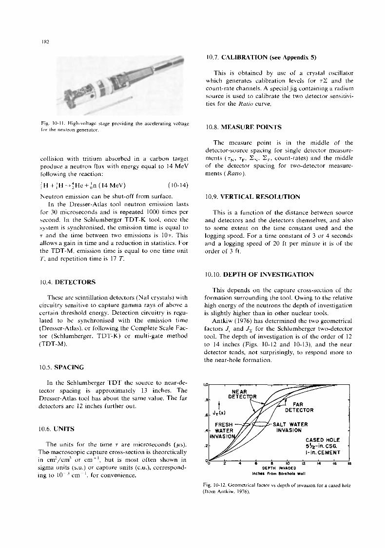
10.7. CALIBRATION (see Appendix 5)
Fig. 10-1 1 . High-voltage stage providing the accelerating voltage f o r the neutron generator.
collision with tritium absorbed in a carbon target produce a neutron flux with energy equal to 14 MeV following the reaction:
f H + i H -:He +bn (14 MeV) (10-14)
Neutron emission can be shut-off from surface. In the Dresser-Atlas tool neutron emission lasts
for 30 microseconds and is repeated 1000 times per aecond. In the Schlumberger TDT-K tool, once the system is synchronised, the emission time is equal to 7 and the time between two emissions is 107. This allows a gain in time and a reduction in statistics. For the TDT-M, emission time is equal to one time unit T. and repetition time is 17 T.
This is obtained by use of a crystal oscillator which generates calibration levels for T X and the count-rate channels. A special jig containing a radium source is used to calibrate the two detector sensitivi- ties for the Ratio curve.
10.8. MEASURE POINTS
The measure point is in the middle of the detector-source spacing for single detector measure- ments ( T ~ , T ~ , Z,, Z,, count-rates) and the middle of the detector spacing for two-detector measure- ments (Ratio).
10.9. VERTICAL RESOLUTION
This is a function of the distance between source and detectors and the detectors themselves, and also to some extent on the time constant used and the logging speed. For a time constant of 3 or 4 seconds and a logging speed of 20 f t per minute it is of the order of 3 f t .
10.10. DEPTH OF INVESTIGATION 10.4. DETECTORS
These are scintillation detectors (NaI crystals) with circuitry sensitive to capture gamma rays of above a certain threshold energy. Detection circuitry is regu- lated to be synchronised with the emission time (Dresser-Atlas), or following the Complete Scale Fac- tor (Schlumberger, TDT-K) or multi-gate method (TDT-M).
10.5. SPACING
In the Schlumberger TDT the source to near-de- tector spacing is approximately 13 inches. The Dresser-Atlas tool has about the same value. The far detectors are 12 inches further out.
10.6. UNITS
The units for the time 7 are microseconds (ps). The macroscopic capture cross-section is theoretically in cm2/cm3 or cm- ' , but is most often shown in sigma units (s.u.) or capture units (c.u.), correspond- ing to lo- ' cm- ' , for convenience.
This depends on the capture cross-section of the formation surrounding the tool. Owing to the relative high energy of the neutrons the depth of investigation is slightly higher than in other nuclear tools.
Antkiw ( 1976) has determined the two geometrical factors J, and J , for the Schlumberger two-detector tool. The depth of investigation is of the order of 12 to 14 inches (Figs. 10-12 and 10-13), and the near detector tends, not surprisingly, to respond more to the near-hole formation.
SALT WATER
CASED HOLE
I-in. CEMENT 5'4-in. CSG.
DEPTH INVADED Inches From eoreholr Wall
4
Fig. 10-12. Geometrical factor vs depth of invasion for a cased hole (from Antkiw. 1976).
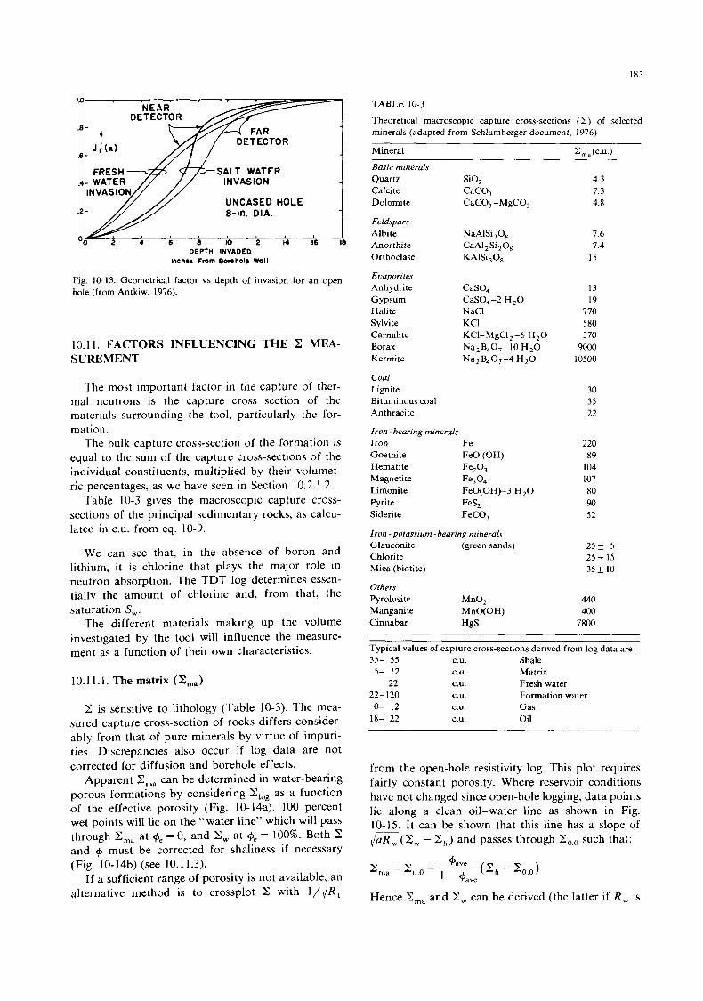
183
1.0 N E A R . - -. . . . I DETECTOR
SALT WATER .4- WATER INVASION
UNCASED HOLE &in. DIA.
b ;O i2 1’4 ie OEPTH INVADED
Inches Fmm Bonholr Wall
Fig. 10-13. Geometrical factor vs depth of invasion for an open hole (from Antkiw, 1976).
10.11. FACTORS INFLUENCING THE 2 MEA- SUREMENT
The most important factor in the capture of ther- mal neutrons is the capture cross section of the materials surrounding the tool, particularly the for- mation.
The bulk capture cross-section of the formation is equal to the sum of the capture cross-sections of the individual constituents, multiplied by their volumet- ric percentages, as we have seen in Section 10.2.1.2.
Table 10-3 gives the macroscopic capture cross- sections of the principal sedimentary rocks, as calcu- lated in C.U. from eq. 10-9.
We can see that, in the absence of boron and lithium, it is chlorine that plays the major role in neutron absorption. The TDT log determines essen- tially the amount of chlorine and, from that, the saturation S,.
The different materials making up the volume investigated by the tool will influence the measure- ment as a function of their own characteristics.
Z is sensitive to lithology (Table 10-3). The mea- sured capture cross-section of rocks differs consider- ably from that of pure minerals by virtue of impuri- ties. Discrepancies also occur if log data are not corrected for diffusion and borehole effects.
Apparent Z,, can be determined in water-bearing porous formations by considering Z,og as a function of the effective porosity (Fig. 10-14a). 100 percent wet points will lie on the “water line” which will pass through Z,, at (p, = 0, and Z, at C#J~ = 100%. Both Z and 4 must be corrected for shaliness if necessary (Fig. 10-14b) (see 10.1 1.3).
If a sufficient range of porosity is not available, an alternative method is to crossplot Z with l / K
TABLE 10-3
Theoretical macroscopic capture cross-sections ( 2 ) of selected minerals (adapted from Schlumberger document, 1976)
Mineral
Basic minerals Quartz SiO, Calcite CaCO, Dolomite CaCO, -MgCO,
Feldspars Albite NaAlSi ,08 Anorthite CaAl , Si ,08 Orthoclase KAISi,O,
Evuporites Anhydrite CaSO, Gypsum CaS0,-2 H,O Halite NaCl Sylvite KCI Carnalite KC1-MgCI2-6 H,O Borax Na,B,O,-10 H,O Kermite Na,B40,-4 H,O
Coal Lignite Bituminous coal Anthracite
Iron -bearing mineruls Iron Fe Goethite FeO (OH) Hematite Fe203 Magnetite F e P 4 Limonite FeO(0H)-3 H,O Pyrite FeS, Siderite FeCO,
Iron -potussium - bearing minerals Glauconite (green sands) Chlorite Mica (biotite)
Others Pyrolusite MnO, Manganite MnO(0H) Cinnabar HgS
z,, (C.U.)
4.3 7.3 4.8
7.6 7.4
15
13 19
770 580 3 70
9000 10500
30 35 22
220 89
104 107 80 90 52
25k 5 25+ I5 35k 10
440 400
7800
Typical values of capture cross-sections derived from log data are: 35- 55 C.U. Shale
5- 12 C.U. Matrix Fresh water 22 C.U.
22- 120 C.U. Formation water
18- 22 C.U. Oil 0- 12 C.U. Gas
from the open-hole resistivity log. This plot requires fairly constant porosity. Where reservoir conditions have not changed since open-hole logging, data points lie along a clean oil-water line as shown in Fig. 10-15. It can be shown that this line has a slope of &(Z, - 2,) and passes through ZO,() such that:
Hence Erna and 2 , can be derived (the latter if R , is
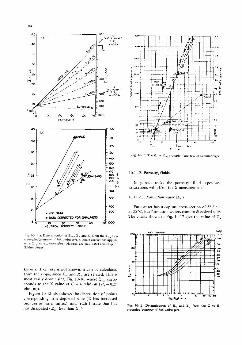
0 POROSITY
110
120
130
140
IS0
160
300
400
500
0 DATA C X R F C X D FOR SHAUNES
10 20 XI 40 NEUTRON POROslTY INDEX
Fig. 10-14 a. Ikterrnination of I,,,.%. 2, and S, from the ZI,, vs $,
cr<ib.+plot (courtesy of Schlumberger). b. Shale corrections applied to a \'I.,e vs $,N crosa-plot (triangles are raw data) (courtesy of Schlumberger).
known. I f salinity is not known, i t can be calculated from the slope, since Z, and R , are related. This is most easily done using Fig. 10-16, where 24,0 corre- sponds to the 2 value at C, = 4 mho/m ( R , = 0.25 ohm-mj).
Figure 10-15 also shows the disposition of points corresponding to a depleted zone ( Z has increased because of water influx), and fresh filtrate that has not dissipated ( less than 2,).
=o 0 ~ I O O 240
1-
Fig. 10-15. The R , vs Z,, , crossplot (courtesy of Schlumberger).
10.1 1.2. Porosity, fluids
In porous rocks the porosity, fluid types and saturations will affect the Z measurement.
10.1 1.2.1. Formation water (ZM,)
Pure water has a capture cross-section of 22.2 C.U.
at 25"C, but formation waters contain dissolved salts. The charts shown in Fig. 10-17 give the value of 2 ,
lZ,D-Z,,,,) in C.U.
Fig. 10-16. Determination of R, and X, from the X vs R, crossplot (courtesy of Schlumberger).
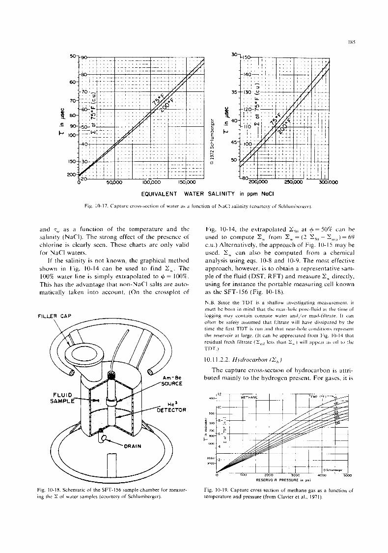
I xs
50
EQUIVALENT WATER SALINITY in ppm NaCl
Fig. 10-17. Capture cross-section of water as a function of NaCl salinity (courtesy of Schlumhcrgcr).
and T, as a function of the temperature and the salinity (NaCl). The strong effect of the presence of chlorine is clearly seen. These charts are only valid for NaCl waters.
I f the salinity is not known, the graphical method shown in Fig. 10-14 can be used to find Z,. The 100% water line is simply extrapolated to + = 100%. This has the advantage that non-NaC1 salts are auto- matically taken into account. (On the crossplot of
Fig. 10-18. Schematic of the SFT-156 sample chamber for measur- ing the Z of water samples (courtesy of Schlumberger).
Fig. 10-14, the extrapolated X 5 , , at $I = 50%' can be used to compute Z, from Z , = (2 Z,,, - Z ,,,,, ) = 69 c.u.) Alternatively, the approach of Fig. 10-15 may be used. Z, can also be computed from a chemical analysis using eqs. 10-8 and 10-9. The most effective approach, however, is to obtain a representative sam- ple of the fluid (DST. RFT) and measure 8 , directly, using for instance the portable measuring cell known as the SFT- 156 (Fig. 10- 18). N.B. Since the T D T is a shallow investigating measurement. i t
must be born in mind that the near-hole pore-fluid at the time of logging may contain connate water and/or mud-filtrate. I t can often be safely assumed that filtrate will have dissipated by the time the first TDT is run and that near-hole conditions represent the reservoir at large. ( I t can be appreciated from Fig. 10.14 that residual fresh filtrate (Z,,,, less than X w ) will appear iis oil to the TDT.)
10.1 1.2.2. H.vdrocurhon (E,, ) The capture cross-section of hydrocarbon i s attri-
buted mainly to the hydrogen present. For gases, it is
e E
I-
10 1000 2000 3000 4000
RESERVOIR PRESSURE in p s i
Fig 10-19 Capture cross-section of methane gas as d function of temperature and pressure (from Clavier et a1 , 1971)
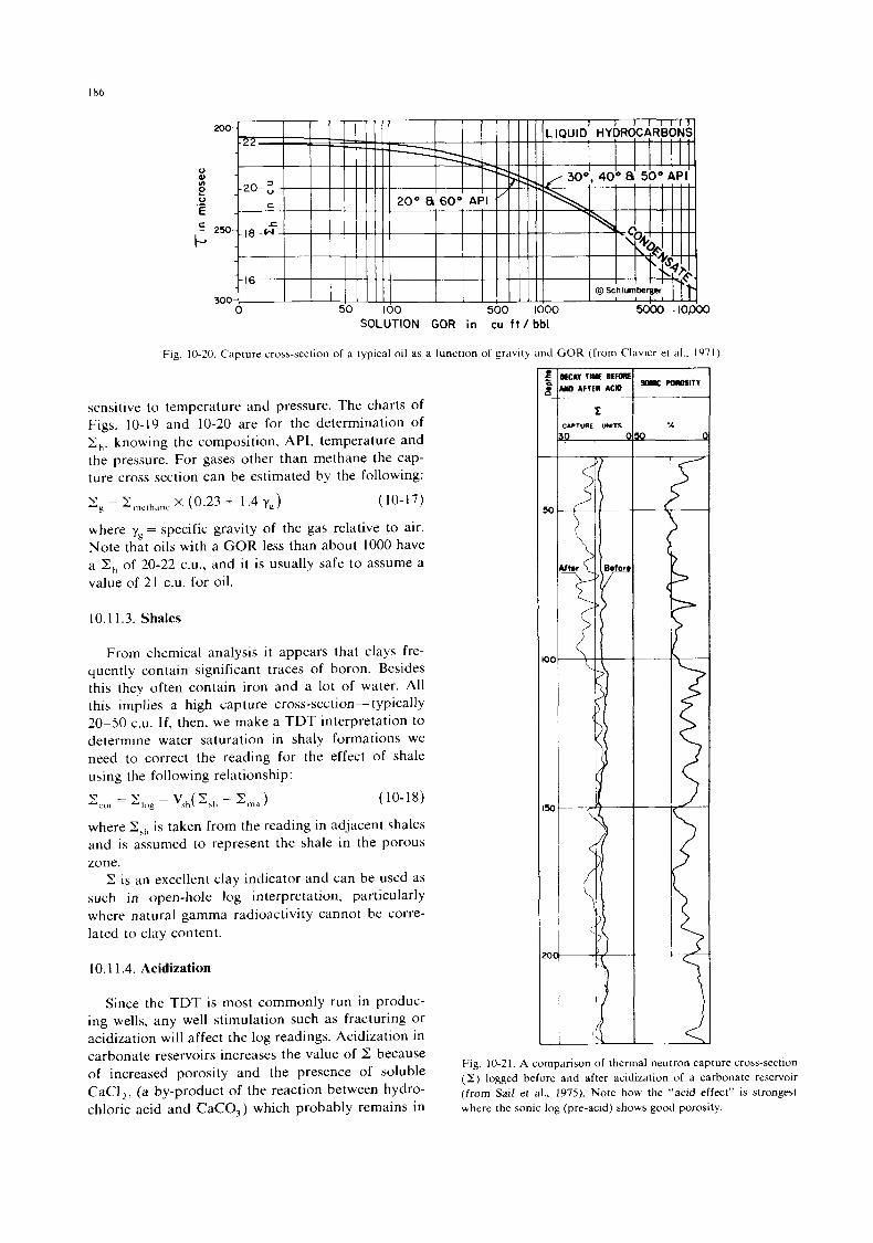
186
SOLUTION GOR in cu f t / bbl
Fig. 10-20. Capture cross-section of a typical oil as a function of gravity and GOR (from Clavier et al.. 1971).
sensitive to temperature and pressure. The charts of Figs. 10-19 and 10-20 are for the determination of 2,,. knowing the composition, API, temperature and the pressure. For gases other than methane the cap- ture cross section can be estimated by the following: \- = 2 x (0.23 + 1.4 y,) (10-17) - p , , l ~ l h a ~ l c
where y, = specific gravity of the gas relative to air. Note that oils with a GOR less than about 1000 have a 2, of 20-22 c.u., and it is usually safe to assume a value of 21 C.U. for oil.
10.1 1.3. Shales
From chemical analysis it appears that clays fre- quently contain significant traces of boron. Besides this they often contain iron and a lot of water. All this implies a high capture cross-section-typically 20-50 C.U. I f , then. we make a TDT interpretation to determine water saturation in shaly formations we need to correct the reading for the effect of shale using the following relationship:
Y,,, = Z,,>g - Y h ( Z \ h - x " , a ) (10-18)
where Z,, is taken from the reading in adjacent shales and is assumed to represent the shale in the porous zone.
Z is an excellent clay indicator and can be used as such in open-hole log interpretation, particularly where natural gamma radioactivity cannot be corre- lated to clay content.
10.1 1.4. Acidization
Since the TDT is most commonly run in produc- ing wells, any well stimulation such as fracturing or acidization will affect the log readings. Acidization in carbonate reservoirs increases the value of Z because Fig. 10-21. A comparison of thermal neutron capture cross-section
( 2 ) logged before and after acidization of a carbonate reservoir (from Saif et a].. 1975). Note how the "acid effect" is strongest
Of increased porosity and the presence Of solub1e CaC12, (a by-product Of the reaction between hydro- chloric acid and CaCO,) which probably remains in where the sonic log (pre-acid) shows good porosity.
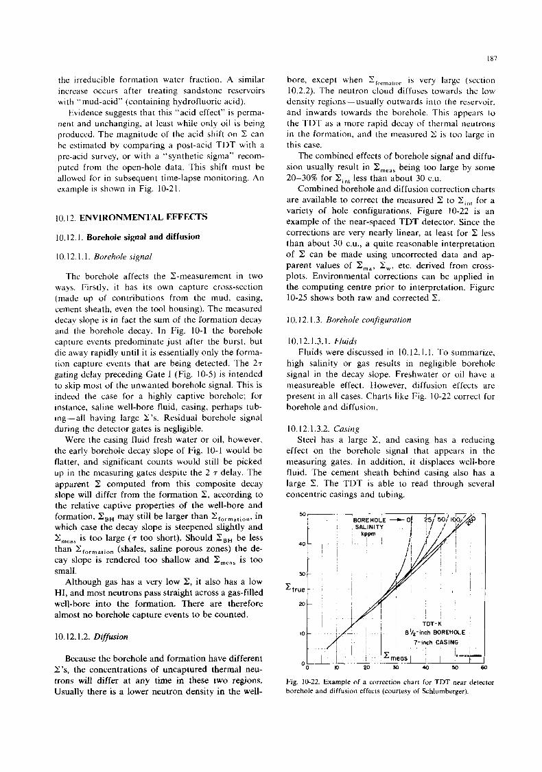
187
the irreducible formation water fraction. A similar increase occurs after treating sandstone reservoirs with “mud-acid” (containing hydrofluoric acid).
Evidence suggests that this “acid effect” is perma- nent and unchanging, at least while only oil is being produced. The magnitude of the acid shift on Z can be estimated by comparing a post-acid TDT with a pre-acid survey, or with a “synthetic sigma” recom- puted from the open-hole data. This shift must be allowed for in subsequent time-lapse monitoring. An example is shown in Fig. 10-21.
10.12. ENVIRONMENTAL EFFECTS
10.12.1. Borehole signal and diffusion
10.12.1.1. Borehole signal
The borehole affects the %measurement in two ways. Firstly, it has its own capture cross-section (made up of contl-ibutions from the mud, casing, cement sheath, even the tool housing). The measured decay slope is in fact the sum of the formation decay and the borehole decay. In Fig. 10-1 the borehole capture events predominate just after the burst, but die away rapidly until it is essentially only the forma- tion capture events that are being detected. The 27 gating delay preceding Gate I (Fig. 10-5) is intended to skip most of the unwanted borehole signal. This is indeed the case for a highly captive borehole; for instance, saline well-bore fluid, casing, perhaps tub- ing-all having large 2 ’s . Residual borehole signal during the detector gates is negligible.
Were the casing fluid fresh water or oil, however, the early borehole decay slope of Fig. 10-1 would be flatter, and significant counts would still be picked up in the measuring gates despite the 2 T delay. The apparent Z computed from thn composite decay slope will differ from the formation Z, according to the relative captive properties of the well-bore and formation. Z,, may still be larger than Zformation, in which case the decay slope is steepened slightly and Z,,,, is too large (7 too short). Should Z,, be less than Zformalion (shales, saline porous zones) the de- cay slope is rendered too shallow and Z,,,, is too small.
Although gas has a very low Z, it also has a low HI, and most neutrons pass straight across a gas-filled well-bore into the formation. There are therefore almost no borehole capture events to be counted.
10.12.1.2. Diffusion
bore, except when EF,,rmdl,on is very large (section 10.2.2). The neutron cloud diffuses towards the low density regions-usually outwards into the reservoir. and inwards towards the borehole. This appears to the TDT as a more rapid decay of thermal neutrons in the formation, and the measured 2: is too large in this case.
The combined effects of borehole signal and diffu- sion usually result in Z,,,, being too large by some 20-30% for Z,,, less than about 30 C.U.
Combined borehole and diffusion correction charts are available to correct the measured Z to Z,,, for a variety of hole configurations. Figure 10-22 is an example of the near-spaced TDT detector. Since the corrections are very nearly linear, at least for Z less than about 30 c.u., a quite reasonable interpretation of Z can be made using uncorrected data and ap- parent values of Z,,, Z,, etc. derived from cross- plots. Environmental corrections can be applied in the computing centre prior to interpretation. Figure 10-25 shows both raw and corrected Z.
10.12.1.3. Borehole configuration
10.12.1.3.1. Fluids Fluids were discussed in 10.12.1.1. To summarize,
high salinity or gas results in negligible borehole signal in the decay slope. Freshwater or oil have a measureable effect. However, diffusion effects are present in all cases. Charts like Fig. 10-22 correct for borehole and diffusion.
10.12.1.3.2. Casing Steel has a large 2, and casing has a reducing
effect on the borehole signal that appears in the measuring gates. In addition, i t displaces well-bore fluid. The cement sheath behind casing also has a large 2. The TDT is able to read through several concentric casings and tubing.
Because the borehole and formation have different Z ’s, the concentrations of uncaptured thermal neu- trons will differ at any time in these two regions. Usually there is a lower neutron density in. the well-
Fig. 10-22. Example of a correction chart for TDT near detector borehole and diffusion effects (courtesy of Schlumberger).
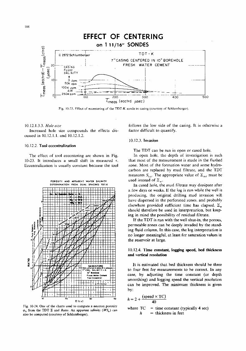
- V
10
v 5
[meas (ecctrd p e c )
Fig. 10-23. Effect of eccentering of the TDT-K sonde in casing (courtesy of Schlumberger)
I
I ~ ~~ FRESH WATER CEMENT _ _ - ___
0 1972 Schlumberger T D T - K
7"CASING CENTERED IN 10" BOREHOLE I
' O - C A S I N G i FLUID SALINITY 1
-
10.12.1.3.3. Hole-size
cussed in 10.12.1.1. and 10.12.1.2.
10.12.2. Tool eccentralization
follows the low side of the casing. It is otherwise a factor difficult to quantify.
10.12.3. Invasion
Increased hole size compounds the effects dis-
The TDT can be run in open or cased hole. The effect of tool eccentering are shown in Fig. In open hole, the depth of investigation is such
10-23. It introduces a small shift in measured 7. that most of the measurement is made in the flushed Eccentralization is usually constant because the tool zone. Most of the formation water and some hydrb-
carbon are replaced by mud filtrate, and the TDT measures &,. The appropriate value of Z,, must be used instead of 8,.
In cased hole, the mud filtrate may dissipate after a few days or weeks. If the log is run while the well is producing, the original drilling mud invasion will have dispersed in the perforated zones, and probably elsewhere provided sufficient time has elapsed. 2 , should therefore be used in interpretation, but keep- ing in mind the possibility of residual filtrate.
If the TDT is run with the well shut-in, the porous, permeable zones can be deeply invaded by the stand- ing fluid column. In this case, the log interpretation is no longer meaningful, at least for saturation values in the reservoir at large.
10.12.4. Time constant, logging speed, bed thickness and vertical resolution
It is estimated that bed thickness should be three to four feet for measurements to be correct. In any case, by adjusting the time constant (or depth smoothing) and logging speed the vertical resolution can be improved. The minimum thickness is given by:
h = 2 +
where TC
(speed x TC) 40 = time constant (typically 4 sec)
h = thickness in feet
Fig. 10-24. One of the charts used to compute a neutron porosity +k from the TDT X and Ratio. An apparent salinity (WS,) can also be computed (courtesy of Schlumberger).
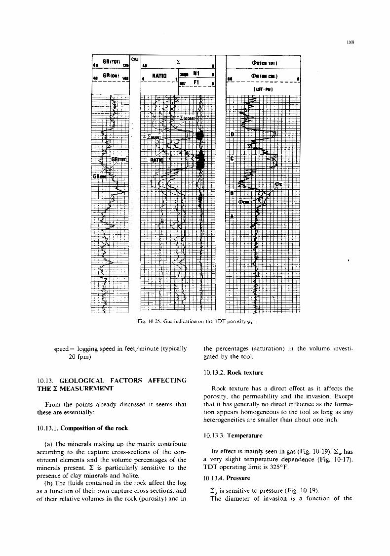
I89
Fig. 10-25. Gas indication on the TDT porosity + k .
speed = logging speed in feet/minute (typically 20 fpm)
10.13. GEOLOGICAL FACTORS AFFECTING THE Z MEASUREMENT
From the points already discussed it seems that these are essentially:
.
the percentages (saturation) in the volume investi- gated by the tool.
10.13.2. Rock texture
Rock texture has a direct effect as it affects the porosity, the permeability and the invasion. Except that it has generally no direct influence as the forma- tion appears homogeneous to the tool as long as any heterogeneities are smaller than about one inch.
10.13.1. Composition of the rock 10.13.3. Temperature
(a) The minerals making up the matrix contribute according to the capture cross-sections of the con- stituent elements and the volume percentages of the minerals present. Z is particularly sensitive to the presence of clay minerals and halite.
(b) The fluids contained in the rock affect the log as a function of their own capture cross-sections, and of their relative volumes in the rock (porosity) and in
Its effect is mainly seen in gas (Fig. 10-19). Z, has a very slight temperature dependence (Fig. 10-1 7). TDT operating limit is 325°F.
10.13.4. Pressure
Z, is sensitive to pressure (Fig. 10-19). The diameter of invasion is a function of the
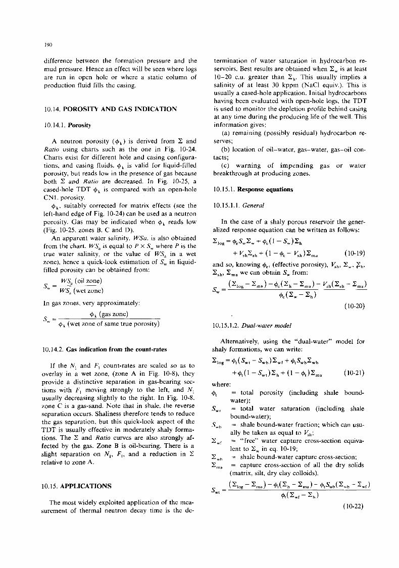
190
difference between the formation pressure and the mud pressure. Hence an effect will be seen where logs are run in open hole or where a static column of production fluid fills the casing.
10.14. POROSITY AND GAS INDICATION
10.14.1. Porosity
A neutron porosity ( G k ) is derived from 2 and Ratio using charts such as the one in Fig. 10-24. Charts exist for different hole and casing configura- tions, and casing fluids. Gk is valid for liquid-filled porosity, but reads low in the presence of gas because both 2 and Ratio are decreased. In Fig. 10-25, a cased-hole TDT Gk is compared with an open-hole CNL porosity.
+ k , suitably corrected for matrix effects (see the left-hand edge of Fig. 10-24) can be used as a neutron porosity. Gas may be indicated when Gk reads low (Fig. 10-25, zones B, C and D).
An apparent water salinity, WSa, is also obtained from the chart. WS, is equal to P X S, where P is the true water salinity, or the value of WSa in a wet zone), hence a quick-look estimation of S, in liquid- filled porosity can be obtained from:
WS, (oil zone) WS;, (wet zone)
s, =
In gas zones, very approximately:
G k (gas zone) s, = + k (wet zone of same true porosity)
10.14.2. Gas indication from the count-rates
If the N , and F, count-rates are scaled so as to overlay in a wet zone, (zone A in Fig. lO-S), they provide a distinctive separation in gas-bearing sec- tions with F, moving strongly to the left, and N , usually decreasing slightly to the right. In Fig. 10-8, zone C is a gas-sand. Note that in shale, the reverse separation occurs. Shaliness therefore tends to reduce the gas separation, but this quick-look aspect of the TDT is usually effective in moderately shaly forma- tions. The Z and Ratio curves are also strongly af- fected by the gas. Zone B is oil-bearing. There is a slight separation on N , , F , , and a reduction in Z relative to zone A.
10.15. APPLICATIONS
The most widely exploited application of the mea- suiement of thermal neutron decay time is the de-
termination of water saturation in hydrocarbon re- servoirs. Best results are obtained when Z, is at least 10-20 C.U. greater than 2,. This usually implies a salinity of at least 30 kppm (NaCl equiv.). This is usually a cased-hole application. Initial hydrocarbons having been evaluated with open-hole logs, the TDT is used to monitor the depletion profile behind casing at any time during the producing life of the well. This information gives:
(a) remaining (possibly residual) hydrocarbon re- serves;
(b) location of oil-water, gas-water, gas-oil con- tacts;
(c) warning of impending gas or water breakthrough at producing zones.
1 0.1 5.1. Response equations
10.15.1.1. General
In the case of a shaly porous reservoir the gener- alized response equation can be written as follows:
'log = +esw'w + Gee(' - sw)'h
+ E h Z s h + - @ e - Eh) 'ma (10-19)
and so, knowing +e, (effective porosity), Kh, Z,, Ch, Z s h , Em, we can obtain S, from:
s, = ('log - 'ma) -+e('h - 'ma) - Kh('sh -
+e('w-'h)
( 10-20)
10.15.1.2. Dual-water model
Alternatively, using the "dual-water'' model for shaly formations, we can write:
'log = +tt(swt - swb)'wf + +tswb'wb
++t( ' -'wt)'h+ ( l -+,)'ma (10-21)
where: = total porosity (including shale bound- water);
S,, = total water saturation (including shale bound-water) ;
S,, = shale bound-water fraction; which can usu- ally be taken as equal to yh;
Z,, = "free" water capture cross-section equiva- lent to 8 , in eq. 10-19;
Z,, = shale bound-water capture cross-section; Zma = capture cross-section of all the dry solids
(matrix, silt, dry clay colloids).
('log - 'ma) - +t('h - 'ma) - +tSwb('wb - 'wf) s,, = G,(',f - 8,)
(10-22)
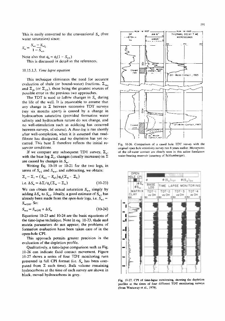
191
)-.RUN I N 1957 .- -RUN I N 1965--------(
This is easily converted to the conventional S, (free water saturation) since:
S w 1 - S w b s, = - 'wh
Note also that +e = &( 1 - S,,) This is discussed in detail in the references.
10.15.1.3. Time lapse equation
This technique eliminates the need for accurate evaluation of shale (or bound-water) fractions, Z,, and Z,, (or Zwb), these being the greatest sources of possible error in the previous two approaches.
The TDT is used to follow changes in S, during the life of the well. It is reasonable to assume that any change in Z between successive TDT surveys (say six months apart) is caused by a change in hydrocarbon saturation (provided formation water salinity and hydrocarbon nature do not change, and no well-stimulation such as acidizing has occurred between surveys, of course). A Base-log is run shortly after well-completion, when it is assumed that mud- filtrate has dissipated, and no depletion has yet oc- curred. This base Z therefore reflects the initial re- servoir conditions.
If we compare any subsequent TDT survey, Z,, with the base log Z,, changes (usually increases) in Z are caused by changes in S,.
Writing Fiq. 10-19 or 10-21 for the two logs, in terms of S,, and S,,, and subtracting, we obtain:
Z n - '1 = ( S w n - S w I ) + e ( Z w - 2,) i.e. AS, = Z, - Z,) (10-23)
We can obtain the actual saturation S,, simply by adding AS, to S,,. Ideally, a good estimate of S,, has already been made from the open-hole logs, i.e. S,, =
s w , = sw,, + AS, ( 10-24)
Equations 10-23 and 10-24 are the basic equations of the time-lapse technique. Note in eq. 10-23, shale and matrix parameters do not appear; the problems of formation evaluation have been taken care of in the open-hole CPI.
This approach permits greater precision in the evaluation of the depletion profile.
Qualitatively, a time-lapse comparison such as Fig. 10-26 can indicate fluid contact movement. Figure 10-27 shows a series of four TDT monitoring runs presented in full CPI format (i.e. S, has been com- puted from Z each time). Bulk volume remaining hydrocarbons at the time of each survey are shown in black, moved hydrocarbons in grey.
s,,,. so:
100 ?50 400
O i l - Water Contocl , 1965
Fig. 10-26. Comparison of a cased hole TDT survey with the original open hole resistivity survey run 8 years earlier. Movements of the oil-water contact are clearly seen in this saline fordation water-bearing reservoir (courtesy of Schlumberger).
(CLAY I 1 -
vsOH 1 v s O H VsOH 1 A O H 50 Ox) 0 50 0 50
4 d 4
...... ....
Fig. 10-27. CPI of time-lapse monitoring, showing the depletion profiles at the times of four different TDT monitoring surveys (from Westaway et al., 1979).
192
10.15.2. Residual oil saturation
Residual Oil Saturation can be estimated in cased-hole or observation wells. Various specialized techniques such as " Log-inject-log'' (see References) have been developed to enhance the accuracy of the ROS evaluation.
10.15.3. Formation fluid
Identification of the formation fluid-gas, oil, water contacts-with the aid of count-rate data, and 2.
10.15.4. Old wells
Evaluation of old wells for possible recompletion, or assessment of initial hydrocarbon reserves. The TDT log provides information on porosity, clay frac- tion, hydrocarbon saturation and type. In an old well where perhaps only an early electrical survey has been run, an evaluation can be made of porosity and initial hydrocarbon reserves with the aid of a TDT log. Gas zones can be identified. Where formation water salinity permits, present-day hydrocarbon saturations can also be estimated.
10.15.5. Supplementary uses
Where bad open-hole conditions prevent a com- prehensive logging suite from being made, the TDT can be run through a drill-pipe, or after completion, to supplement the logging data (lithology, porosity, hydrocarbons).
Although rarely run in open hole, the TDT can be used alongside other tools to give a better definition of the lithology, particularly the clay fraction. An obvious application here would be in shaly carbonate reef deposits, where the clay fraction does not gener- ally correlate with the GR (unless the NGS is run).
10.16. REFERENCES
Antkiw, S., 1976. Depth of investigation of the dual-spacing ther- mal neutron decay time loggmg tool. SPWLA 17th Annu. Log. Symp. Trans., Paper CC.
Boyeldieu, C. and Horvath, S., 1980. A contribution to the evalua- tion of residual oil from well logs for tertiary recovery. SPWLA 21st Annu. Log. Symp., Trans.
Clavier, C., Hoyle, W.R. and Meunier, D., 1969. Quantitative interpretation of T D T Logs, paper SPE 2658 presented at the SPE 44th Annu. Meet., Denver, Sept. 28-Oct. I , 1969. J. Pet. Technol., June 197 1.
Dewan, J.T., Johnstone, C.W., Jacobson, L.A., Wall, W.B. and Alger, R.P., 1973. Thermal neutron decay time logging using dual detection. Log Analyst 145): 13.
Edmundson, H. and Dadrian, C., 1973. Thermal neutron decay time logging applications in the Eastern Hemisphere. 2nd Annu. Symp. SAID, Paris, Oct.
Edmundson. H. and Raymer, L., 1979. Radioactive logging param- eters for common minerals. SPWLA 20th Annu. Log. Symp. Trans.
F e d , W.H., 1972. Occurrence of the neutron-absorbing tracing element boron. Part 11-boron in oil-field water. The Log Analyst, Vol. XIII, Jan-Feb, 1972.
Golder, D., 1978. Thermal decay time logging at Ekofisk. case study of a multiple use tool. European Offshore Petroleum Conference and Exhibition, Paper No. EUR 91.
Hall, J., Tittman, J. and Edmundson, H., 1981. A system for wellsite measurement of Z fluid. SPWLA. 21st Annu. Log. Symp. Trans., Paper W.
Hall, J.. Johnstone, C.. Baldwin, J. and Jacobson, L., 1980. A new thermal neutron decay logging system-TDT-M. SPE of AIME. Paper No. SPE 9462.
Jameson, J.B., McGhee. B.F., Blackburn, J.S. and Leach, B.C., 1977. Dual spacing T D T applications in marginal conditions. J. Pet. Technol., Sept.
Kidwell. C. and Guillory, A,, 1980. A recipe for residual oil saturation determination J. Pet. Technol. Nov.
Locke, S.. and Smith, R., 1975. Computed departure curves for the thermal neutron decay time log. SPWLA, 16th Annu. Log. Symp. Trans.
McGhee, B.F., McCuire, J.A. and Vacca, H.L., 1974. Examples of dual spacing thermal neutron decay time logs in Texas Coast oil and gas reservoirs. SPWLA 15th Annu. Log. Symposium. Trans., Houston, Paper R.
Nelligan, W.B. and Antkiw, S., 1976. Accurate thermal neutron decay time measurements with the dual-spacing TDT--$ laboratory study. 51st Annu. Fall Techn. Conf. SPE/AIME, Paper SPE 5 156.
Nelligan, W.B., Wahl, J.S., Frentrop, A.H., Johnstone, C.W. and Schwartz. R.J., 1970. The thermal neutron decay time log. SOC. Pet. Eng., J. Dec: 365-380.
Preeg, W.E. and Scott, H.D., 1981. Computing thermal neutron decay time (TDT) environmental effects using Monte Carlo techniques. Paper SPE 10293 presented at the SPE 56th Annual Technical Conference and Exhibition, San Antonio, Oct. 4-7, 1981.
Rinehart, C.E. and Weber, H.J., 1975. Measuring thermal neutron absorption cross sections of formation water. SPWLA 16th Annu. Log. Symp. Trans. June, 1975.
Robinson, J.D., 1974. Neutron decay time in the subsurface: theory, experiment, and an application to residual oil de- termination. SOC. Pet. Eng. of AIME 49th Annu. Fall Meet., Houston, October 6-9, 1974, Paper SPE 5 119.
Saif, A.S., Cochrane, J.E., Edmundson, H.N. and Youngblood, W.E., 1975. Analysis of pulsed-neutron' decay-time logs in acidized carbonate formations. SPE J., Dec. Paper No. SPE 5443.
Schlumberger, 1974. Log Interpretation; Vol. 11-Applications. Schlumberger, Mar., 1976. The Essentials of Thermal Decay Time
Logging. Schlumberger, Mar., 1980. Dual-Water Model Cased Reservoir
Analysis. Serpas, C.J., Wickmann, P.A., Fertl, W.H., Devries, M.R. and
Randall, R.R., 1977. The dual detector neutron lifetime log-theory and practical applications. SPWLA 18th Annu. Log. Symp. Trans., Houston Paper CC.
Smith, R.L. and Patterson, W.F., 1976. Production management of reservoirs through log evaluation. SPE of AIME, Paper No. SPE 5507.
SPWLA, 1976. Pulsed Neutron Logging, Reprint Volume. Tittman, J., 1956. Radiation Logging. Fundamentals of Logging,
University of Kansas.

193
Tixier, M.P. and Vesperman, F.A. 1976. The porosity transform-A shale-compensated interpretation using T D T and neutron Logs, SPWLA 17th Annu. Log. Symp., Trans., Paper GG.
Westaway, P., Wittman, M. and Rochette, P., 1979. Application of Nuclear Techniques to Reservoir Monitoring. SPE of AIME, Paper No. SPE 7776.
Wahl, J.S., Nelligan, W.B., Frentrop, A.H., Johnstone, C.W. and
Schwartz. R.J., 1970. The thermal neutron decay time log. SPE J., Dec.
Youmans, A.H., Hopkinson, E.C. and Wichmann. P.A.. 1966. Neutron lifetime logging in theory and practice SPWLA Sev- enth Annual Logging Symposium, May 8-1 I , Tulsa, Eq. 5.
Youngblood, W.E., 1980. The application of pulsed neutron decay time logs to monitor water floods with changing salinity. SPE of AIME, Paper No. 7771.

This Page Intentionally Left Blank
195
11. FORMATION DENSITY MEASUREMENTS (the gamma-gamma log or density log)
1 1.1. PRINCIPLE
The formation is subjected to gamma rays emitted by a special source (60Co or 13’Cs). Gamma rays are particles having no mass and moving at the speed of light. These gamma rays or photons collide with matter in three different types of interaction, depen- ding on their incident energy.
have an energy of 0.51 MeV and are emitted in almost exactly opposite direction (Fig. 11-2).
The pair production cross-section increases with increasing energy (Fig. 11-5). It is directly propor- tional to Z 2 ( Z being the atomic number).
The influence of pair production is negligeable for the types of source used in density tools.
1 1.1.2. Compton scattering 1 1.1.1. Pair production
When the photon energy is above 1.02 MeV, the interaction of photon and matter leads to pair produc- tion, it means the production of a negutron (%r nega- tive electron) and a positron (or positive electron), each with an energy of 0.51 MeV (Fig. 11-1).
These two previously non-existent electron masses appear as a result of the disappearance of the photon energy. All of the photon energy is given up to the two electrons, with the exception of a very small amount going into the recoiling nucleus. The reaction is: hv, - ei + e- + 2T ( 1 1-1)
This phenomenon can only occur when the energy of the photon is higher than 2mc2 ( = 1.02 MeV). Re- quirement of conservation of energy and momentum of the system allow this process to occur only in the electric field of a nucleus.
After the pair has been created, positron and electron lose energy by ionization as they move off from the point of origin. When the positron energy becomes low it annihilates by combination with an electron in a process that is the reverse of that by which it was created: e+ + e- + 2hv
It means that the rest energy of the two mutually annihilating particles is transformed into radiant en- ergy. The two photons, or gamma rays, in eq. 11-2 are called annihilation radiation. The two photons
(1 1-2)
Fig. 11-1. Schematic of pair production at a nucleus.
When the incident photon collides with an elec- tron (Fig. 11-3) its energy hv, is divided between the kinetic energy B = mv2 given to the electron ejected from its atom with initial velocity o and a photon “scattered” in a direction making an angle 8 with the original incident direction.
This elastic collision between the gamma ray and an individual electron simply allows the gamma ray to proceed, deflected by its encounter, but reduczd in energy. This process occurs mainly with outer elec- trons of the atoms.
This type of reaction is called Compton scattering and it is the reaction figuring mainly in density measurements. The scattering effect is sensitive to the electron density of the formation (number of elec- trons per unit volume). This is developed in Para- graph 11-2.
An important feature of Compton scattering is that if the incident energy of the gamma ray, E,, is known, then the scattering angle 8 and the scattered gamma ray energy, E,, are quite simply related (Fig. 1 1-3).
1 1.1.3. Photo-electric effect
In the course of a collision with an electron a photon can transfer all its energy to the electron in the form of kinetic energy. The electron is ejected from its atom and the photon disappears. The gamma ray is absorbed (Fig. 1 1-4).
The microscopic cross-section of this reaction, T ,
has been found to be related to the atomic number of the target atom, Z,.and the energy of the incident gamma ray, E,, by the following relation:
2 4 . 6
7 = 12.1- barns/atom ( E,)3’Is
( 1 1-3)
The photo-electric effect is highest when the gamma-
196
Fig. 11-2. Cloud chamber photograph of pair production with track curvatures produced by a field of 1500 gauss (in Lapp and Andrews, 1972).
Compton recoil electron
Fig. 11-3. Schematic of the Compton process. Geometrical rela- tions in the Compton process.
e- ted
photoelectron
Fig. 11-4. Schematic of the photoelectric process
.
p .01 8
.001 I-I
01 .1 1 10 Energy of gamma rays (MeV)
Fig. 11-5. Gamma ray mass absorption coefficient over the energy range of interest in Formation Density Logging (from Tittman and Wahl, 1965).
ray energy is small and the atomic number of the element high.
The relative importance of the three major types of interactions between photon and matter for different photon energies and for different atomic numbers is represented by the schematic diagram of Fig. 11-5. The lines indicate the values of absorber atomic number, Z , and photon energy at which neighbohg effects are equally probable.
If we compare the mass absorbtion factor p with the energy of the gamma rays (Fig. 11-5) we can see that for an energy band of 0.2-2.0 MeV absorption is due essentially to Compton scattering.
The density tool measures the intensity of scattered gamma rays at a fixed distance from the source.
T h s intensity is smaller the larger the number of collisions experienced by a photon, hence when the electron density is higher. To. a first approximation the electron density is proportional to the density of the formation. Hence, the number of gamma rays detected is smaller when the formation density is higher.
So, in dense formations few gamma rays are de- tected since the number of collisions is high and gamma rays are absorbed (photo-electric effect) hav- ing lost a proportion of their energy in each collision. In low-density formations few collisions are made and so less energy is lost. More gamma rays are detected.
1 1.2. ABSORPTION EQUATION
If L is large enough the intensity of the gamma rays is an exponential function of the electron density of the formation and is given by the equation:
I = Ioe-’PcL (1 1-4)
197
TABLE 1 1 - 1
Values of C = 2 Z / A for the most common elements
Element Z A 2 Z / A
H C N 0 Na Mg A1 Si P S C1 K Ca Fe Ba
1 6 7 8
11 12 13 14 15 16 17 19 20 26 56
1.0079 12.01 11 14.0067 15.9994 22.9898 24.312 26.98 15 28.086 30.9738 32.064 35.453 39.102 40.08 55.847
137.34
1.9843 0.9991 0.9995 1 .Ooo 0.9569 0.9872 0.9636 0.9969 0.9686 0.998 0.959 0.9718 0.998 0.93 1 1 0.8155
where: I = intensity of gamma rays measured at the detec-
I , =intensity of gamma rays at the source. p , =electronic density of the formation in the inter-
val L (number of electrons per unit volume). L = detector-source spacing. p is, to a first approximation, a constant depending on the tool geometry, the energy of the gamma rays emitted by the source and the detector characteristics.
L,I = L,r, - p p e ~ (1 1-5)
which says in effect that the electron density is a linear function of logarithm of the intensity of gamma rays detected.
tor.
Taking natural logarithms of eq. 11-4 gives:
11.3. THE RELATION BETWEEN THE ELEC- TRONIC DENSITY AND THE BULK DENSITY
The bulk density (pb) of the formation is what we seek to determine. This is related to the electron density ( p , ) by the following:
p e = P b ( Z / A ) N (1 1-6) where: Z = atomic number A = atomic mass N = Avogadro’s number (6.02 X For the majority of elements and constituents of rocks ( Z / A ) is very close to 0.5 except for hydrogen for which it is almost 1 (Tables 11-1 and 11-2).
( pe )i = 2pe/N (1 1-7)
As the tool is calibrated in a freshwater-saturated limestone the apparent global density pa is linked to ( P,)~ by the equation: pa = 1.07( pe)i - 0.1883 (1 1-8)
For sands, limestones and dolomites (liquid saturated) pa is practically equal to pb. For some substances or for gas-filled formations corrections have to be made (Fig. 11-6).
We define an electron density index by:
1 I .4. GAMMA-RAY SOURCES
The most widely used are: 60Cobalt which emits photons at energies of 1.17
I3’Cesium that emits photons of energy 0.66 MeV. and 1.33 MeV.
TABLE 11-2 Values of C , electronic and bulk densities of the most common minerals found in rocks
Compound Formula Actual 2ZZ’s Electronic density Apparent density density mol.wt. (as seen by tool) Pb Pe Pa
Quartz Si02 2.654 0.9985 2.650 2.648 Calcite CaCO, 2.710 0.9991 2.708 2.710 Dolomite CaCO, MgCO, 2.870 0.9977 2.863 ‘2.876 Anhydnte CaSO, 2.960 0.9990 2.957 2.977 Sylvite KCI 1.984 0.9657 1.916 1.863 Halite NaCl 2.165 0.9581 2.074 2.032 Gypsum CaSO, 2 H 2O 2.320 1.0222 2.372
1.442 { 1.852 Anthracite coal 1.030 { 1.400
1.800
2.351 { 1.355
1.7% 1.272 1.173
‘1.590 { 1.514
Salt water 200.000 ppm 1.146 1.0797 1.237 1.135 “ oil” 4 C H d 0.850 1.1407 0.970 0.850
1.060 1.200
{ 1.500 Bituminous coal
Fresh water H2O 1 .Ooo 1.1101 1.110 1 .oo
Methane CH4 pmst h I .247 Pmcth 1.335 ~ ~ ~ h - 0 . 1 8 8 “GaS”
, . lH4.2 9 1.238 1.238 pg 1.325 pg-0.188
198
+.I4
+ . I2
+ 0.1
+ .08
+ .06
+.04
t.02
0
- .02
-.04
Fig. 11-6. Corrections to be applied to apparent bulk density, plo,. in order to derive true density, ph. (from Tittman and Wahl, 1965).
1 1.5. DETECTORS
These are scintillation detectors set to detect gamma rays above a certain energy level.
1 1.6. CALIBRATION UNITS
The initial laboratory calibrations are made in pure limestone saturated with freshwater, where the density is known exactly.
Secondary calibrations are made in blocks of aluminium and sulphur or magnesium. Finally, at the wellsite a cahbration jig is used that gives a radioac- tivity level of known intensity designed to test the detection system.
Originally the units of measurement were the standard counts per sec (Schlumberger) or the stan- dard unit of density (PGAC). These were then trans- formed to density by charts given by the service companies. However, since the introduction of two detector tools the transformation is made inside the surface instrumentation and the log is given directly in grams per cubic centimeter: ,g/cm3.
spring, the measurement suffered from the effects of mud-cake, its type, thickness and density.
To eliminate mud-cake effects service companies now offer two-detector systems in so-called com- pensated tools (Fig. 11-8). The corrections are made within the surface equipment as a function of the readings from the two detectors. Figure 11-9, known as the spine- and ribs plot, shows that for a given value of pb, the readings from the two detectors fall on an average curve, whatever the density or thick- ness of the mud-cake. By using the set of curves it is
- - Detector
Spacing
------Source 11.7. THE TOOLS
The first tools used only one detector (Fig. 11-7). Although pushed against the borehole wall by a
Fig. 11-7. Principle and schematic of the one detector formation density tool.
199
Fig. 11-8. Schematic of the Dual-spacing formation density log (FDC) (courtesy of Schlumberger).
possible to determine the correction Ap,. The log presents both p,, and the correction applied Apb.
11.8. DEPTH OF INVESTIGATION
This is lower the higher is the density of the rock. Figure 11-10 gives an idea of the investigated zone. We can see that it is small and does not go above 6 inches. In porous and permeable formations the den- sity tool investigates essentially the invaded zone.
W I- a a
5 (3
I- z 3 0 u
0 I- u W I- W
0
0
In
0 z 0 -1
a
n
z 2
7 YUDCAKE
W I T H 0 A R I T E
91 ~~ ~
SHORT SPACING DETECTOR COUNTING RATE
Fig. 11-9. "Spine-and-ribs" plot, showing response of FDC count- ing rates to mud cake (from Wahl et al., 1964) (courtesy of SPE of AIME).
0.8C
DEPTH SATURATED Inches From Borehole Wall
100
35% WROSrrY OPEN HOLE
pb APP B U N DENS
12 DEPTH SATURATED
Inches From Borehole Wall
Fig. 1 1-10, Pseudo-geometrical factor (J-factor) curves for FDC density tool. for 22% and 35% porosity (from Sherman and Lock, 1975, courtesy of SPE of AIME). . 1 1.9. VERTICAL RESOLUTION
For single-detector tools it corresponds to the source-detector spacing, around 16 inches for the FDL. For two-detector tools the distance between the detectors (span) gives the resolution, about 10 inches for the FDC.
1 1.10. MEASURE POINT
This is either at the midpoint of the source-detec- tor spacing (FDL one-detector system) or the mid- point of the two detector span (FDC or two-detector system).
1 1.1 1. FUNDAMENTAL FACTORS INFLUENC- ING THE MEASUREMENT
We have seen that for a given source and spacing the main factors are the bulk density and the ratio Z / A .
As a first approximation Z / A is considered a constant. The global density in the region investi- gated by the tool depends then on: (a) the density and percentage of different mineralogical con- stituents in the rock; and (b) in the case of porous rocks, the density of the different fluids and their
200
-
-
-
percentage in the reservoir (porosity) and in the pore space (saturation). However, a correct interpretation implies that we take account of the influence Z / A as this differs from 1 for oil, gas and water (see Table 1 1-2).
We should consider in particular the influence on the measurement of three important parameters.
.3
.2
- 0
1 1 . 1 1.2. Water
The fluid in the zone investigated by the tool is mainly mud filtrate, if the rock is porous and in- vaded. As the density of this can vary with temper- ature and pressure as a function of its salinity, we need to make corrections in the interpretation (Fig. 11-1 1).
1 1 . 1 1 . 1 . Shales 1 1 . 1 1.3. Hydrocarbon
If we try to interpret the density in terms of porosity the influence of shale for density logs is much less than for neutron logs. The density of "dry" clays is somewhere around that of quartz and so they have approximately the same effect within the matrix.
In any case when an interpretation is made for lithology or porosity it is preferable to take into account the effect of shales, above all if their density is very different from the other minerals composing the rock. We have the following equation: P b c = P b + K h ( & n a - & h ) (1 1-9)
where: pbc = shale corrected bulk density; pb pma =matrix bulk density; psh = shale bulk density; V,, = shale percentage.
=log reading of bulk density;
TEMPERATURE (CENTIGRADE)
I20 I 20
I15 I I 5
I10 I10
I I
g IM 105 ::
k - E - b 100 100:
, n ,
> r
z z W W n
095
0 90 090
1 1 1 , ~ , I l , l l i ; ! . l i , 085 ' ' 1 1 ' ' I ' I ' " ' I I OBS
40 100 200 300 400 440
TEMPERATURE (FAHRENHEIT)
Fig. 11-11. Densities of water and NaCl solution at varying tem- peratures and pressures (courtesy of Schlumberger).
Hydrocarbon densities, especially gas, are less than that of water (Fig. 11-12), which means that the same formation full of gas appears much lighter and there- fore more porous than if water-saturated. There is a case for making a hydrocarbon correction especially when determining porosity. If we write Apbh for the variation in density caused by hydrocarbons we can write:
P h = P h c + 'Phh (1 1-10)
where: pbc = bulk density corrected for hydrocarbon (i.e.
where the pores are saturated with mud filtrate P m f ) ;
pb =bulk density log reading. It can be shown that Apbh is given by: A P h h = @ s h r ( c m f p m f - c h p h ) (1 1-1 1 )
P b c = P h + 1 .07@shr (cmfpmf- c h p h ) (1 1-12) and hence
GAS PRESSURE x 1000 in psi0
Fig. 11-12. Gas density and hydrogen index as a function of pressure and temperature for a gas mixture slightly heavier than methane (CI . , H4,2) (courtesy of Schlumberger).
20 1
with: + shr
C m i Ch
P h P m r
11.12.
= porosity; = hydrocarbon residual saturation in invaded
= electronic density coefficient for mud-filtrate; =electronic density coefficient for hydro-
=hydrocarbon density; =mud filtrate density.
zone;
carbon;
INTERPRETATION
The bulk density is exactly equal to the sum of the densities of the component parts of the formation multiplied by their respective percentage volume. For a porous formation, this implies: P b = + P f + ( l - + ) P m a (11-13)
with (11-14)
(1 1-15)
(1 1-16)
(1 1-17)
Equation 11-13 can be rewritten in terms of porosity as
+ D = ( Pma - P b )/( P m a - Pmf ) (1 1-18)
with +,, = porosity; pman =bulk density of mineral n; s x 0 =water saturation in the invaded zone; v, = volumic percentage of mineral n . The chart in Fig. 11-13 shows this relation.
In general for most fluids, with the exception of gas or light hydrocarbons, and most minerals malung up a rock pb is obtained directly from the apparent pa
T ae
0 1 11 2 1 1 4 1
Fig. 11-13. Relationshp between $I and pb knowing the density of the mineral (p,.).
given by the tool (the coefficient C being nearly equal to 1).
In the case of a gas or light hydrocarbon forma- tion where the coefficient C is no longer near l, this has to be taken into account when + is calculated. It can be shown that eq. 11-3 may be rewritten as:
P log = - .0704 (P [ c m a P m a - h rch P h - sxocm f P m I 1 + P m (1 1-19)
and that eq. 11-18 becomes:
1 1.13. ENVIRONMENTAL EFFECTS
1 1.13.1. Time constant, recording speed, dead time, bed thickness
These factors have been dealt with in the general discussion of nuclear logs (Chapter 5).
1 1.13.2. The borehole
The effect of the borehole is easily seen for uncom- pensated density logs but less so for the compens'ated (Fig. 11-14). Several factors are important.
MUD - FILLED HOLES
,o .eel APPARENT FORMATION DENSITY
1 I 1 I
6"-9" 1 0 ' 11" 1 2 13" 1 4 15"
BORE. HOLE DIAMETER
GAS FILLED HOLES
APPARENT FORMATION DEWITY
ga% 10" 11" 12" 13" 1 4 ' 15" 1
BORE. HOLE DIAMETER
Fig. 11-14. Corrections for hole size (from Wahl et al., 1964; courtesy of SPE of AIME).
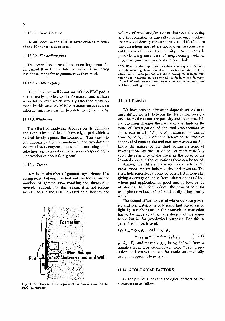
202
1 1.13.2.1. Hole diameter
Its influence on the FDC is more evident in holes above 10 inches in diameter.
11.13.2.2. The drillingfluid
The corrections needed are more important for air- drilled than for mud-drilled wells, as air, being less dense, stops fewer gamma rays than mud.
1 1.13.2.3. Hole rugosity
If the borehole well is not smooth the FDC pad is not correctly applied to the formation and isolates zones full of mud which strongly affect the measure- ment. In this case, the FDC correction curve shows a different influence on the two detectors (Fig. 11-15).
11.13.3. Mud-cake
The effect of mud-cake depends on its thickness and type. The FDC has a sharp-edged pad which is pushed 'firmly against the formation. This tends to cut through part of the mud-cake. The two-detector system allows compensation for the remaining mud- cake layer up to a certain thickness corresponding to a correction of about 0.15 g/cm3.
1 1.13.4. Casing
Iron is an absorber of gamma rays. Hence, if a casing exists between the tool and the formation, the number of gamma rays reaching the detector is severely reduced. For this reason, it is not recom- mended to run the FDC in cased hole. Besides, the
wall
Fig. 11-15. Influence of the rugosity of the borehole wall on the FDC log response.
volume of mud and/or cement between the casing and the formation is generally not known. It follows that revised density measurements are difficult since the corrections needed are not known. In some cases calibration of cased hole density measurements is possible using core data of neighbouring wells or repeat sections run previously in open hole. N.B. When making repeat sections there may appear differences with the main log above those due to statistical variations. This is often due to heterogeneous formations having for example frac- tures, vugs or fissures more on one side of the hole than the other. If the FDC pad does not trace the same path on the two runs there will be a resulting difference.
11.13.5. Invasion
We have seen that invasion depends on the pres- sure difference A P between the formation pressure and the mud column, the porosity and the permeabil- ity. Invasion changes the nature of the fluids in the zone of investigation of the tool (replacement of none, part or all of R , by R m f , saturations ranging from S, to S,,). In order to determine the effect of the invaded zone on the tool measurement we need to know the nature of the fluid within its zone of investigation. By the use of one or more resistivity tools the resistivity of the water in the pores of the invaded zone and the saturations there can be found.
Among the different environmental effects the most important are hole rugosity and invasion. The first, hole rugosity, can only be corrected empirically, giving a density obtained from other sections of hole where pad application is good and is low, or by attributing theoretical values (the case of salt, for example) or values defined statistically using nearby wells.
The second effect, universal where we have poros- ity and permeability, is only important where gas or light hydrocarbons are in the reservoir. A correction has to be made to obtain the density of the virgin formation ie. for geophysical purposes. For this, a general equation is used:
(PtJcor = @,Pw + 441 - S,)P,
+ <hPsh -k ( l - @ - K h > p m a (1 1-21)
+, S.,,, Kh and possibly pma being defined from a quantitative interpretation of well logs. This interpre- tation and correction can be made automatically using an appropriate program.
1 1.14. GEOLOGICAL FACTORS
As for previous logs the geological factors of im- portance are as follows:
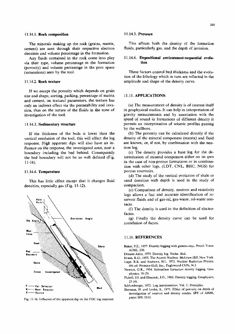
1 1.14.1. Rock composition
203
11.14.5. Pressure
The minerals making up the rock (grains, matrix, cement) are seen through their respective electron densities and volume percentage in the formation.
Any fluids contained in the rock come into play via their type, volume percentage in the formation (porosity) and volume percentage in the pore space (saturations) seen by the tool.
11.14.2. Rock texture
If we except the porosity which depends on grain size and shape, sorting, packing, percentage of matrix and cement, on textural parameters, the texture has only an indirect effect via the permeability and inva- sion, thus on the nature of the fluids in the zone of investigation of the tool.
1 1.14.3. Sedimentary structure
If the thickness of the beds is lower than the vertical resolution of the tool, this will affect the log response. High apparent dips will also have an in- fluence on the response, the investigated zone, near a boundary including the bed behind. Consequently the bed boundary will not be so well defined (Fig. 11-16).
1 1.14.4. Temperature
This has little effect except that it changes fluid densities, especially gas (Fig. 1 1 - 12).
This affects both the density of the formation fluids, particularly gas, and the depth of invasion.
1 1.14.6. Depositional environment-sequential evolu- tion
These factors control bed thickness and the evolu- tion of the lithology which in turn are reflected in the amplitude and shape of the density curve.
1 1.15. APPLICATIONS
(a) The measurement of density is of interest itself in geophysical studies. It can help in interpretation of gravity measurements and by association with the speed of sound in formations of different density it permits an interpretation of seismic profiles passing by the wellbore.
(b) The porosity can be calculated directly if the density of the mineral component (matrix) and fluid are known, or, if not, by combination with the neu- tron log.
(c) The density provides a base log for the de- termination of mineral component either on its gwn in the case of non-porous formations or in combina- tion with other logs, (LDT, CNL, BHC, NGS) for porous reservoirs.
(d) The study of the vertical evolution of shale or sand densities with depth is used in the study of compaction.
(e) Comparison of density, neutron and resistivity logs allows a fast and accurate identification of re- servoir fluids and of gas-oil, gas-water, oil-water con- tact s.
( f ) The density is used in the definition of electro- facies.
(8) Finally the density curve can be used for correlation of facies.
1 \
1 1.16. REFERENCES
F- Far O e t i c i o r N-Near D e t e c t o r S - S o u r c e
-::\ Mud \ Fig. 11-16. Influence of the apparent dip on the FDC log response.
Baker, P.E., 1957. Density logging with gamma-rays. Petrol. Trans.
Dresser-Atlas, 1973. Density log. Techn. Bull. Evans, R.D., 1955. The Atomic Nucleus. McGraw-Hill, New York. Lapp, R.E. and Andrews, H.L. 1972. Nuclear Radiation Physics,
Newton, G.R., 1954. Subsurface formation density logging. Geo-
Pickell, J.J. and Heacock, J.G., 1960. Density logging. Geophysics,
Schlumberger, 1972. Log interpretation. Vol. 1 : Principles. Sherman, H. and Locke, S., 1975. Effect of porosity on depth of
investigation of neutron and density sondes. SPE of AIME, paper SPE 5510.
AIME, 210.
4th ed. Prentice-Hall, Inc., Englewood Cliffs, N.J.
physics, 19 (3).
25 (4).

204
Tittman, J. and Wahl, J.S., 1965. The physical foundation of formation density logging (Gamma-Gamma). Geophysics, 30
Wahl, J.S., Tittman, J., Johnstone, C.W. and Alger. R.P. (1964). The dual spacing formation density log. J. Pet. Technol., 16
(2). (12).
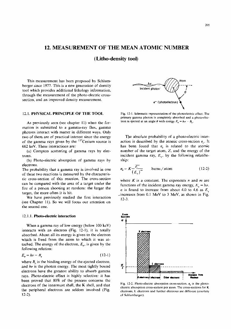
205
12. MEASUREMENT OF THE MEAN ATOMIC NUMBER
(Litho-density tool)
This measurement has been proposed by Schlum- berger since 1977. This is a new generation of density tool which provides additional lithology information, through the measurement of the photo-electric cross- section, and an improved density measurement.
12.1. PHYSICAL PRINCIPLE OF THE TOOL
As previously seen (see chapter 11) when the for- mation is submitted to a gamma-ray flux, gamma photons interact with matter in different ways. Only two of them are of practical interest since the energy of the gamma rays given by the '37Cesium source is 662 keV. These interactions are:
(a) Compton scattering of gamma rays by elec- trons.
(b) Photo-electric absorption of gamma rays by electrons. The probability that a gamma ray is involved in one of these two reactions is measured by the characteris- tic cross-section of t h s reaction. The cross-section can be compared with the area of a target under the fire of a person shooting at random: the larger the target, the more often it is hit.
We have previously studied the first interaction (see Chapter 11). So we will focus our attention on the second one.
12.1.1. Photo-electric interaction
When a gamma ray of low energy (below 100 keV) interacts with an electron (Fig. 12-l), it is totally absorbed. About all its energy is given to the electron which is freed from the atom to which it was at- tached. The energy of the electron, E,, is given by the following relation: E, = hv - Be (12-1)
where Be is the binding energy of the ejected electron, and hv is the photon energy. The most tightly bound electrons have the greatest ability to absorb gamma rays. Photo-electric effect is highly selective: i t has been proved that 80% of the process concerns the electrons of the innermost shell, the K shell, and that the peripheral electrons are seldom involved (Fig. 12-2).
e- (photoelectron)
Fig. 12-1. Schematic representation of the photoelectric effect. The primary gamma photon is completely absorbed and a photo-elec- tron is ejected at an angle 8 with energy E, = h v - B,.
The absolute probability of a photo-electric inter- action is described by the atomic cross-section a,. It has been found that a, is related to the atomic number of the target atom, Z , and the energy of the incident gamma ray, E,, by the following r e l a t h - ship:
a, = K--, barns/atom ( 12-2) Z"
( E J
where K is a constant. The exponents n and rn are functions of the incident gamma ray energy, E, = hv. n is found to increase from about 4.0 to 4.6 as E,
,increases from 0.1 MeV to 3 MeV, as shown in Fig. 12-3.
Cross Sections
I
Fig. 12-2. Photo-electric absorption cross-section. oe is the photo- electric absorption cross-section per atom. The cross-sections for K electrons, L electrons and further electrons are different (courtesy of Schlumberger).
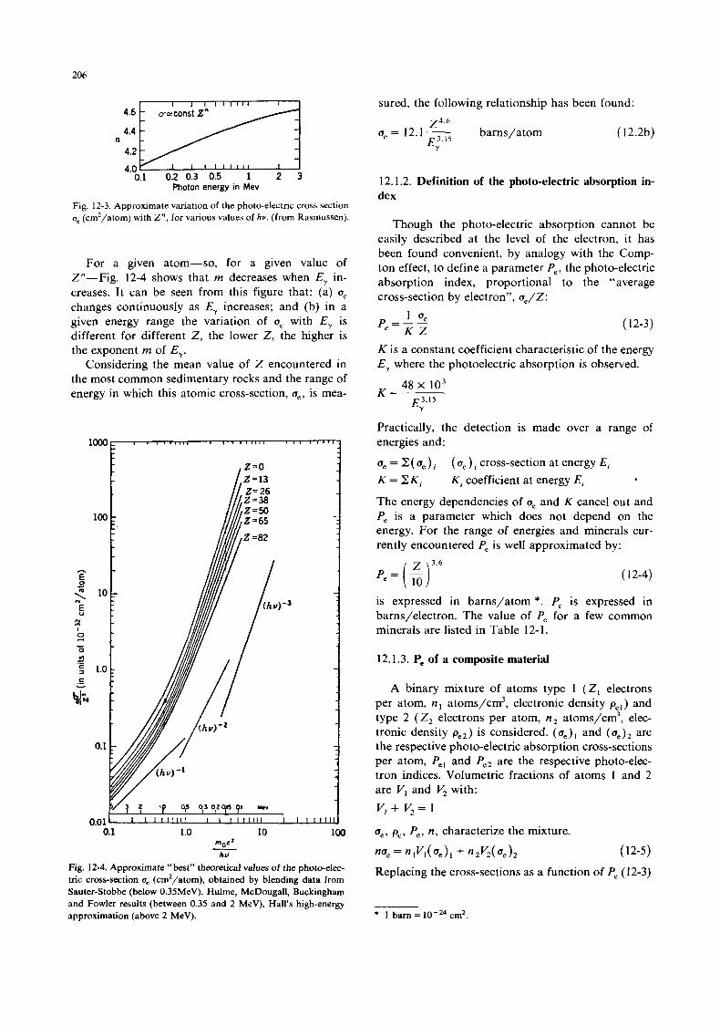
206 n41v 4.2
4.0 0.1 02 0.3 0.5 1 2 3 .~
Photon energy in Mev
Fig. 12-3. Approximate variation of the photo-electric cross section a, (cm2/atom) with Z”, for various values of hv. (from Rasmussen).
For a given atom-so, for a given value of Z“-Fig. 12-4 shows that m decreases when E, in- creases. It can be seen from this figure that: (a) u, changes continuously as E, increases; and (b) in a given energy range the variation of a, with E, is different for different Z , the lower Z , the higher is the exponent m of E,.
Considering the mean value of Z encountered in the most common sedimentary rocks and the range of energy in which this atomic cross-section, a,, is mea-
0.1 1 .o 10 100 m , y
hL, -
Fig. 12-4. Approximate “best” theoretical values of the photo-elec- tnc cross-section ue (cm2/atom), obtained by blending data from Sauter-Stobbe (below 0.35MeV). Hulme, McDougall, Buckingham and Fowler results (between 0.35 and 2 MeV), Hall’s high-energy approximation (above 2 MeV).
sured, the following relationship has been found:
a, = 12.1 - barns/atom (12.2b) Z4.h
E13.I5
12.1.2. Definition of the photo-electric absorption in- dex
Though the photo-electric absorption cannot be easily described at the Ievel of the electron, i t has been found convenient, by analogy with the Comp- ton effect, to define a parameter P,, the photo-electric absorption index, proportional to the “average cross-section by electron”, u,/Z:
1 ‘e p =-- K Z
( 12-3)
K is a constant coefficient characteristic of the energy E, where the photoelectric absorption is observed.
K - 48 x 103
E Y
Practically, the detection is made over a range of energies and:
a, = Z (u,), (u,) , cross-section at energy El K = ZK, K , coefficient at energy El
The energy dependencies of a, and K cancel out and P, is a parameter which does not depend on the energy. For the range of energies and minerals cur- rently encountered P, is well approximated by:
p e = ( $ ) ( 12-4)
is expressed in barns/atom *. P, is expressed in barns/electron. The value of P, for a few common minerals are listed in Table 12- 1.
3.6
12.1.3. P, of a composite material
A binary mixture of atoms type 1 (2, electrons per atom, n , atoms/cm3, electronic density p,,) and type 2 (Z, electrons per atom, n 2 atoms/cm3, elec- tronic density pe2) is considered. (u,)~ and (u , )~ are the respective photo-electric absorption cross-sections per atom, Pel and Pe2 are the respective photo-elec- tron indices. Volumetric fractions of atoms 1 and 2 are Vl and V2 with: V , + V , = l
a,, p,, P,, n , characterize the mixture. = nlVl(ue)l+ “ 2 ‘ 2 ( ~ e ) 2 ( 12-5)
Replacing the cross-sections as a function of P, (12-3)
* 1 barn = cm2.
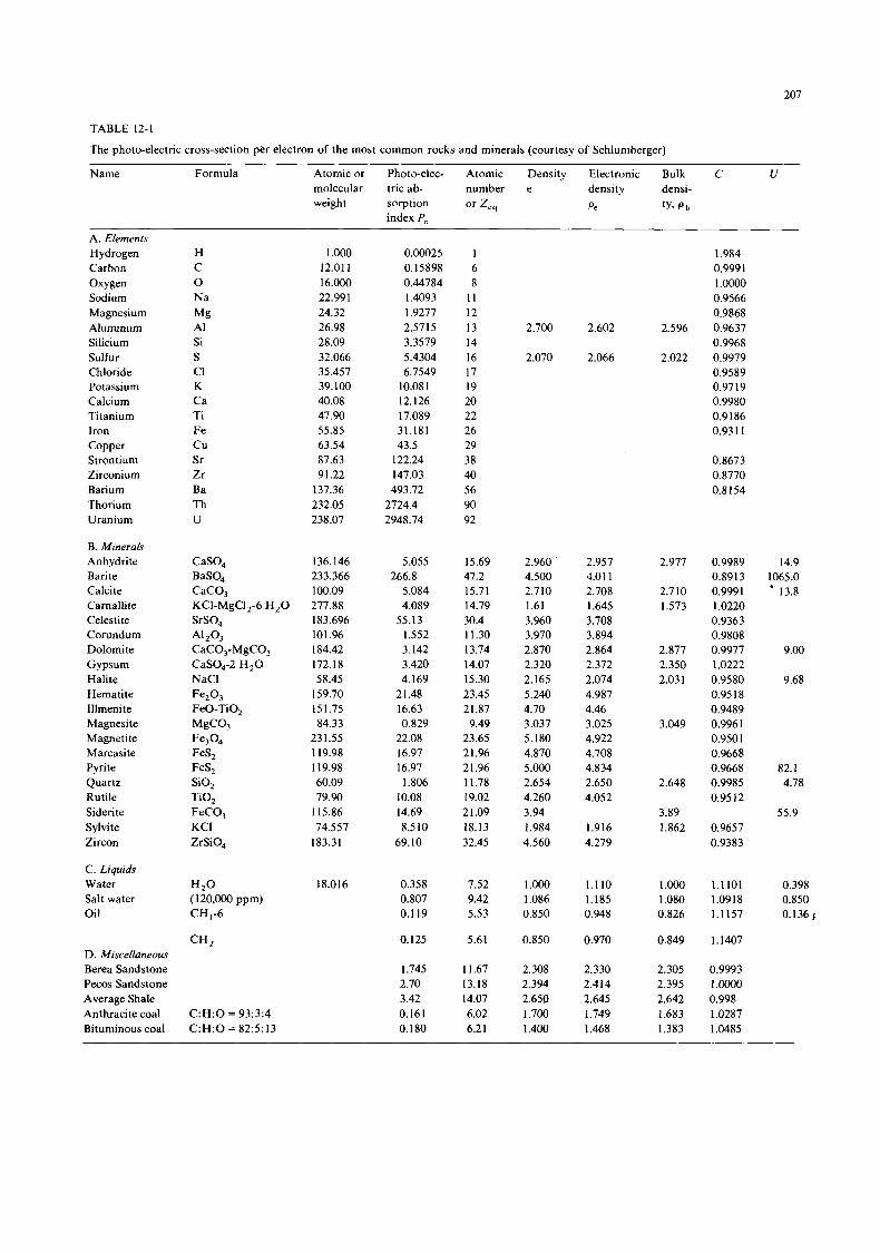
207
TABLE 12-1
The photo-electric cross-section per electron of the most common rocks and minerals (courtesy of Schlurnberger)
Name Formula Atomic or Photo-elec- Atomic Density Electronic Bulk C U molecular tric ab- number e weight sorption or Z,,
index P,
A. Elements Hydrogen Carbon Oxygen Sodium Magnesium Aluminum Silicium Sulfur Chloride Potassium Calcium Titanium Iron Copper Strontium Zirconium Barium Thorium Uranium
B. Minerals Anhydrite Barite Calcite Carnallite Celestite Corundum Dolomite Gypsum Halite Hematite Illmenite Magnesite Magnetite Marcasite Pyrite Quartz Rutile Siderite Sylvite Zircon
C. Liquids Water Salt water Oil
D. Miscellaneous Berea Sandstone Pecos Sandstone Average Shale Anthracite coal Bituminous coal
H C 0 Na Mg A1 Si S C1 K Ca Ti Fe c u Sr Zr Ba Th U
CaSO, BaSO, CaCO, KCI-MgC12-6 H,O SrSO,
CaC0,-MgCO, CaS0,-2 H,O NaCl
FeO-TiO,
A1203
MgCO, Fe3 0 4
FeS, FeS, SiO, TiO, FeCO, KCI ZrSiO,
1.000 12.01 1 16.000 22.99 1 24.32 26.98 28.09 32.066 35.457 39.100 40.08 47.90 55.85 63.54 87.63 91.22
137.36 232.05 238.07
136. I46 233.366 100.09 277.88 183.696 101.96 184.42 172.18 58.45
159.70 151.75 84.33
231.55 119.98 119.98 60.09 79.90
115.86 74.557
183.31
C:H:O = 93:3:4 C:H:O = 82:5:13
0.00025 0.15898 0.44784 1.4093 1.9277 2.5715 3.3579 5.4304 6.7549
10.08 1 12.126 17.089 31.181 43.5
122.24 147.03 493.72
2724.4 2948.74
5.055
5.084 4.089
1.552 3.142 3.420 4.169
266.8
55.13
21.48 16.63
22.08 16.97 16.97
10.08 14.69
69.10
0.829
1.806
8.5 10
0.358 0.807 0.119
0.125
1.745 2.70 3.42 0.161 0.180
1 6 8
11 12 13 14 16 17 19 20 22 26 29 38 40 56 90 92
15.69 47.2 15.71 14.79 30.4 11.30 13.74 14.07 15.30 23.45 21.87
9.49 23.65 21.96 21.96 11.78 19.02 2 1.09 18.13 32.45
7.52 9.42 5.53
5.61
11.67 13.18 14.07 6.02 6.21
2.700
2.070
2.960 4.500 2.710 1.61 3.960 3.970 2.870 2.320 2.165 5.240 4.70 3.037 5.180 4.870 5.000 2.654 4.260 3.94 1.984 4.560
1.000 1.086 0.850
0.850
2.308 2.394 2.650 1.700 1.400
density P,
2.602
2.066
2.957 4.01 1 2.708 1.645 3.708 3.894 2.864 2.372 2.074 4.987 4.46 3.025 4.922 4.708 4.834 2.650 4.052
1.916 4.279
1.110 1.185 0.948
0.970
2.330 2.414 2.645 1.749 1.468
densi- ty, P b
2.596
2.022
2.977
2.710 1.573
2.877 2.350 2.03 1
3.049
2.648
3.89 1.862
1 .Ooo 1.080 0.826
0.849
2.305 2.395 2.642 1.683 1.383
1.984 0.9991 1 .oooo 0.9566 0.9868 0.9637 0.9968 0.9979 0.9589 0.9719 0.9980 0.9 186 0.93 1 1
0.8673 0.8770 0.8 I54
0.9989 0.8913 0.9991 1.0220 0.9363 0.9808 0.9977 1.0222 0.9580 0.95 18 0.9489 0.996 1 0.9501 0.9668 0.9668 0.9985 0.9512
0.9657 0.9383
1.1101 1.0918 1.1157
1.1407
0.9993 I .oooo 0.998 1.0287 1.0485
14.9 1065.0 ' 13.8
9.00
9.68
82.1 4.78
55.9
0.398 0.850 0.136 (
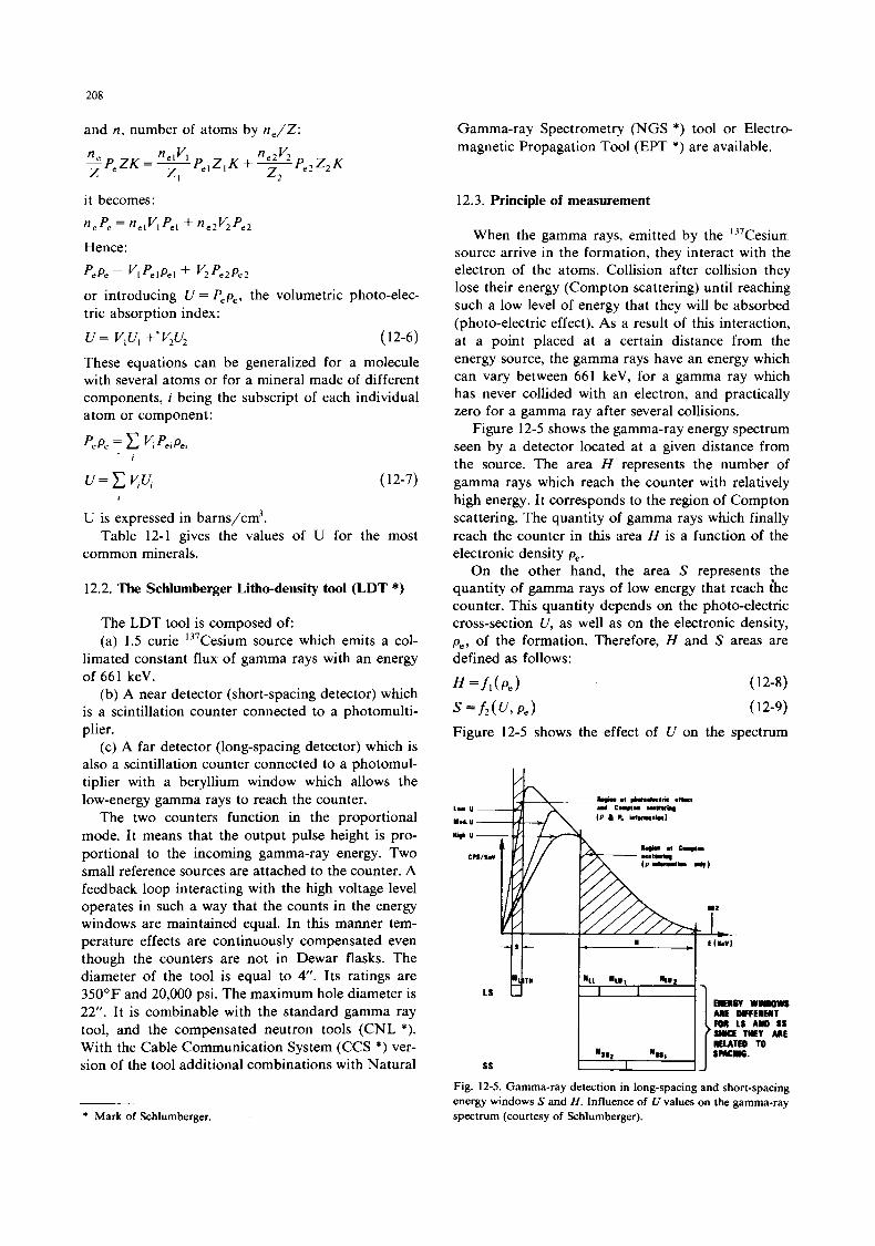
208
and n , number of atoms by n , / Z :
i t becomes :
nepe = nelVlPel + ne2'2Pe2
Hence:
P e p , = V l P e l P e I + V 2 P e 2 ~ e 2
or introducing U = Pepe, the volumetric photo-elec- tric absorption index:
u = vp, +' v2u2 ( 12-6)
These equations can be generalized for a molecule with several atoms or for a mineral made of different components, i being the subscript of each individual atom or component:
Pe Pe = C pa pel I
U = C Y U , I
( 12-7)
U is expressed in barns/cm3.
common minerals. Table 12-1 gives the values of U for the most
12.2. The Schlumberger Litho-density tool (LDT *)
The LDT tool is composed of: (a) 1.5 curie 137Cesium source which emits a col-
limated constant flux of gamma rays with an energy of 661 keV.
(b) A near detector (short-spacing detector) which is a scintillation counter connected to a photomulti- plier.
(c) A far detector (long-spacing detector) which is also a scintillation counter connected to a photomul- tiplier with a beryllium window which allows the low-energy gamma rays to reach the counter.
The two counters function in the proportional mode. It means that the output pulse height is pro- portional to the incoming gamma-ray energy. Two small reference sources are attached to the counter. A feedback loop interacting with the high voltage level operates in such a way that the counts in the energy windows are maintained equal. In this manner tem- perature effects are continuously compensated even though the counters are not in Dewar flasks. The diameter of the tool is equal to 4". Its ratings are 350'F and 20,000 psi. The maximum hole diameter is 22". It is combinable with the standard gamma ray tool, and the compensated neutron tools (CNL *). With the Cable Communication System (CCS *) ver- sion of the tool additional combinations with Natural
Gamma-ray Spectrometry (NGS *) tool or Electro- magnetic Propagation Tool (EPT *) are available.
12.3. Principle of measurement
When the gamma rays, emitted by the '37Cesiurr source arrive in the formation, they interact with the electron of the atoms. Collision after collision they lose their energy (Compton scattering) until reaching such a low level of energy that they will be absorbed (photo-electric effect). As a result of t h s interaction, at a point placed at a certain distance from the energy source, the gamma rays have an energy which can vary between 661 keV, for a gamma ray which has never collided with an electron, and practically zero for a gamma ray after several collisions.
Figure 12-5 shows the gamma-ray energy spectrum seen by a detector located at a given distance from the source. The area H represents the number of gamma rays which reach the counter with relatively high energy. It corresponds to the region of Compton scattering. The quantity of gamma rays which finally reach the counter in this area H is a function of the electronic density pe.
On the other hand, the area S represents the quantity of gamma rays of low energy that reach {he counter. This quantity depends on the photo-electric cross-section U, as well as on the electronic density, p,, of the formation. Therefore, H and S areas are defined as follows:
H = fi ( P e ) ( 12-8) S=fi(u, P e l ( 12-9)
Figure 12-5 shows the effect of U on the spectrum
ss
* Mark of Schlumberger.
Fig. 12-5. Gamma-ray detection in long-spacing and short-spacing energy windows S and H. Influence of (I values on the gamma-ray spectrum (courtesy of Schlumberger).
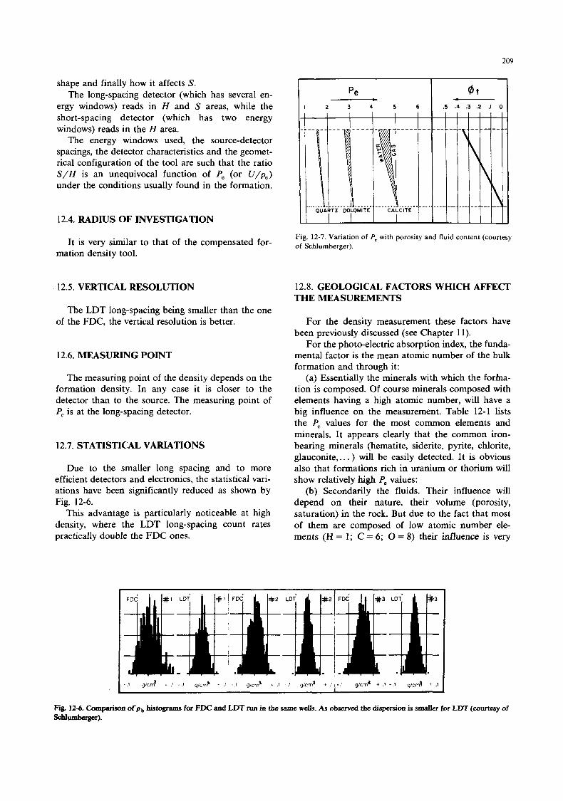
209
shape and finally how it affects S. The long-spacing detector (which has several en-
ergy windows) reads in H and S areas, while the short-spacing detector (which has two energy windows) reads in the H area.
The energy windows used, the source-detector spacings, the detector characteristics and the geomet- rical configuration of the tool are such that the ratio S / H is an unequivocal function of P, (or U/p, ) under the conditions usually found in the formation.
12.4. RADIUS OF INVESTIGATION
It is very similar to that of the compensated for- mation density tool.
12.5. VERTICAL RESOLUTION
The LDT long-spacing being smaller than the one of the FDC, the vertical resolution is better.
12.6. MEASURING POINT
The measuring point of the density depends on the formation density. In any case it is closer to the detector than to the source. The measuring point of P, is at the long-spacing detector.
12.7. STATISTICAL VARIATIONS
Due to the smaller long spacing and to more efficient detectors and electronics, the statistical vari- ations have been significantly reduced as shown by Fig. 12-6.
This advantage is particularly noticeable at high density, where the LDT long-spacing count rates practically double the FDC ones.
Pe b
2 3 4 5 6 .5 : .3 .2 .I 0 I
Fig. 12-7. Variation of P, with porosity and fluid content (courtesy of Schlumberger).
12.8. GEOLOGICAL FACTORS WHICH AFFECT THE MEASUREMENTS
For the density measurement these factors have been previously discussed (see Chapter 11).
For the photo-electric absorption index, the funda- mental factor is the mean atomic number of the bulk formation and through it:
(a) Essentially the minerals with which the forha- tion is composed. Of course minerals composed with elements having a high atomic number, will have a big influence on the measurement. Table 12-1 lists the P, values for the most common elements and minerals. It appears clearly that the common iron- bearing minerals (hematite, siderite, pyrite, chlorite, glauconite,. . . ) will be easily detected. It is obvious also that formations rich in uranium or thorium will show relatively high P, values:
(b) Secondarily the fluids. Their influence will depend on their nature, their volume (porosity, saturation) in the rock. But due to the fact that most of them are composed of low atomic number ele- ments (H = 1; C = 6; 0 = 8) their influence is very
Fig. 12-6. Comparison of pb histograms for FDC and LDT run in the same wells. As observed the dispersion is smaller for LDT (courtesy of schlumberger).
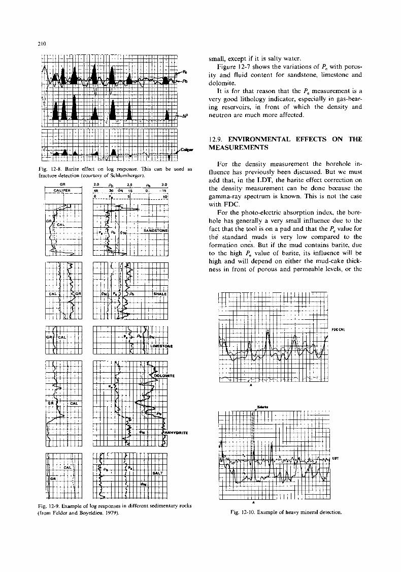
210
Fig. 12-8. Barite effect on log response. This can be used as fracture detection (courtesy of Schlumberger).
GR
E
Fig. 12-9. Example of log responses in different sedimentary rocks (from Felder and Boyeldieu, 1979).
small, except if it is salty water. Figure 12-7 shows the variations of P, with poros-
ity and fluid content for sandstone, limestone and dolomite.
It is for that reason that the P, measurement is a very good lithology indicator, especially in gas-bear- ing reservoirs, in front of which the density and neutron are much more affected.
12.9. ENVIRONMENTAL EFFECTS ON THE MEASUREMENTS
For the density measurement the borehole in- fluence has previously been discussed. But we must add that, in the LDT, the barite effect correction on the density measurement can be done because the gamma-ray spectrum is known. This is not the case with FDC.
For the photo-electric absorption index, the bore- hole has generally a very small influence due to the fact that the tool is on a pad and that the P, value for the standard muds is very low compared to the formation ones. But if the mud contains barite, due to the high P, value of barite, its influence will be high and will depend on either the mud-cake thick- ness in front of porous and permeable levels, or the
A
Fig. 12-10. Example of heavy mineral detection
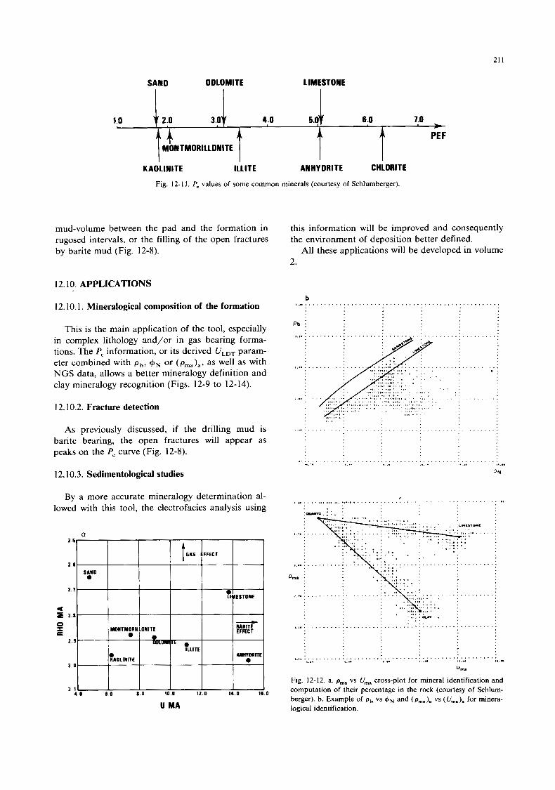
21 1
DOLOMITE LIMESTONE SAND
y 2.0 3.0v 4.0 5.0” 6.0 1.0 1.0
A A A PEF MONTMORILLONITE t 4
I KAOLlNlTE ILLITE ANHY DRlTE CHLORITE
Fig. 12- 1 1. P, values of some coinmon minerals (courtesy of Schlumberger).
mud-volume between the pad and the formation in rugosed intervals, or the filling of the open fractures by barite mud (Fig. 12-8).
this information will be improved and consequently the environment of deposition better defined.
All these applications will be developed in volume 2.
12.10. APPLICATIONS b
12.10.1. Mineralogical composition of the formation
This is the main application of the tool, especially in complex lithology and/or in gas bearing forma- tions. The P, information, or its derived U,,, param- eter combined with pb, +,., or (P,,,~)~, as well as with NGS data, allows a better mineralogy definition and clay mineralogy recognition (Figs. 12-9 to 12-14).
12.10.2. Fracture detection
As previously discussed, if the drilling mud is barite bearing, the open fractures will appear as peaks on the P, curve (Fig. 12-8).
12.10.3. Sedimentological studies
By a more accurate mineralogy determination al- lowed with this tool, the electrofacies analysis using
GAS EFFECT
2 6
2 .1
0
U M A
ON
. . . . . . . . . . . . . . . . . . . . . . . . . . . . . . . . . . . . . . . . . . . . . . . . . . . . . . . . . . . . . . .
, . , , . ~ . . . . . . . . . . . . . . . . . . . . . . . . . . . . . . . . . . . . . . . . . . . . . . . . . . . .
. . . . . . . . . . . . . . . . . . . . . . . . . . . . . . . . . . . . . . . . . . . . . . . . . . 11.1. / I _ . . t..”
Fig. 12-12. a. pma vs Urn, cross-plot for mineral identification and computation of their percentage in the rock (courtesy of Schlum- berger). b. Example of pb vs +N and vs (Urn.). for minera- logical identification.
..a. ..” I .. urn,
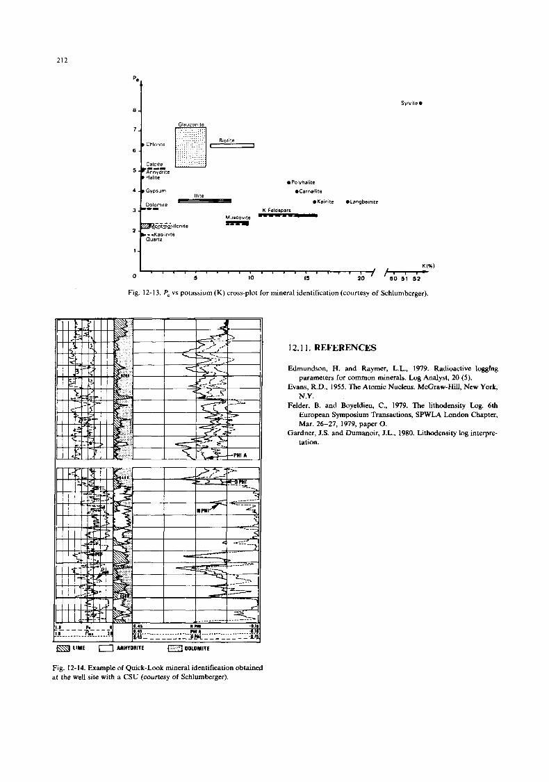
212
pe
8 -
7 -
6 -
5
4
B Chlorite
Calcite - v Z G Z t e
B Halite
- D Gypsum
Svlviie.
1.
Glauconite
............. ............. ............. Blotlie - ..... .......... . . . . . . . . . . . . . . . . . . . . . . . . . . . . . . . . . . . 1. . . . . . . . . . . .
.Polyhalite
.Carnalltte lll ite
___c_ mKarnite WLangbetnite
12.1 1. REFERENCES
Edmundson, H. and Raymer, L.L., 1979. Radioactive logghg parameters for common minerals. Log Analyst, 20 ( 5 ) .
Evans, R.D., 1955. The Atomic Nucleus. McGraw-Hill, New York, N.Y.
Felder, B. and Boyeldieu, C., 1979. The lithodensity Log. 6th European Symposium Transactions, SPWLA London Chapter, Mar. 26-27, 1979, paper 0.
Gardner, J.S. and Dumanoir, J.L., 1980. Lithodensity log interpre- tation.
LIME a ANHYORITE DOLOMITE
Fig. 12- 14. Example of Quick-Look mineral identification obtained at the well site with a CSU (courtesy of Schlumberger).
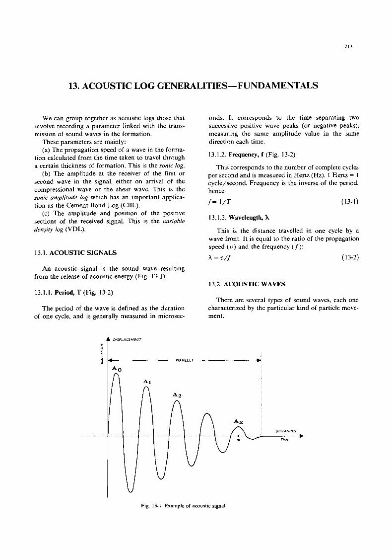
213
13. ACOUSTIC LOG GENERALITIES-FUNDAMENTALS
We can group together as acoustic logs those that involve recording a parameter linked with the trans- mission of sound waves in the formation.
These parameters are mainly: (a) The propagation speed of a wave in the forma-
tion calculated from the time taken to travel through a certain thickness of formation. T h s is the sonic log.
(b) The amplitude at the receiver of the first or second wave in the signal, either on arrival of the compressional wave or the shear wave. This is the sonic amplitude log which has an important applica- tion as the Cement Bond Log (CBL).
(c) The amplitude and position of the positive sections of the received signal. This is the variable denSity log (VDL).
13.1. ACOUSTIC SIGNALS
onds. It corresponds to the time separating two successive positive wave peaks (or negative peaks), measuring the same amplitude value in the same direction each time.
13.1.2. Frequency, f (Fig. 13-2)
This corresponds to the number of complete cycles per second and is measured in Hertz (Hz). 1 Hertz = 1 cycle/second. Frequency is the inverse of the period, hence f = 1/T (13-1)
13.1.3. Wavelength, X
This is the distance travelled in one cycle by a wave front. It is equal to the ratio of the propagation speed ( u ) and the frequency ( f ):
h = u/f ( 13-2)
An acoustic signal is the sound wave resulting . from the release of acoustic energy (Fig. 13-1).
13.1.1. Period, T (Fig. 13-2) 13.2. ACOUSTIC WAVES
There are several types of sound waves, each one characterized by the particular kind of particle move- ment.
The period of the wave is defined as the duration of one cycle, and is generally measured in microsec-
4 DISPLACEMENT
Fig. 13-1. Example of acoustic signal.
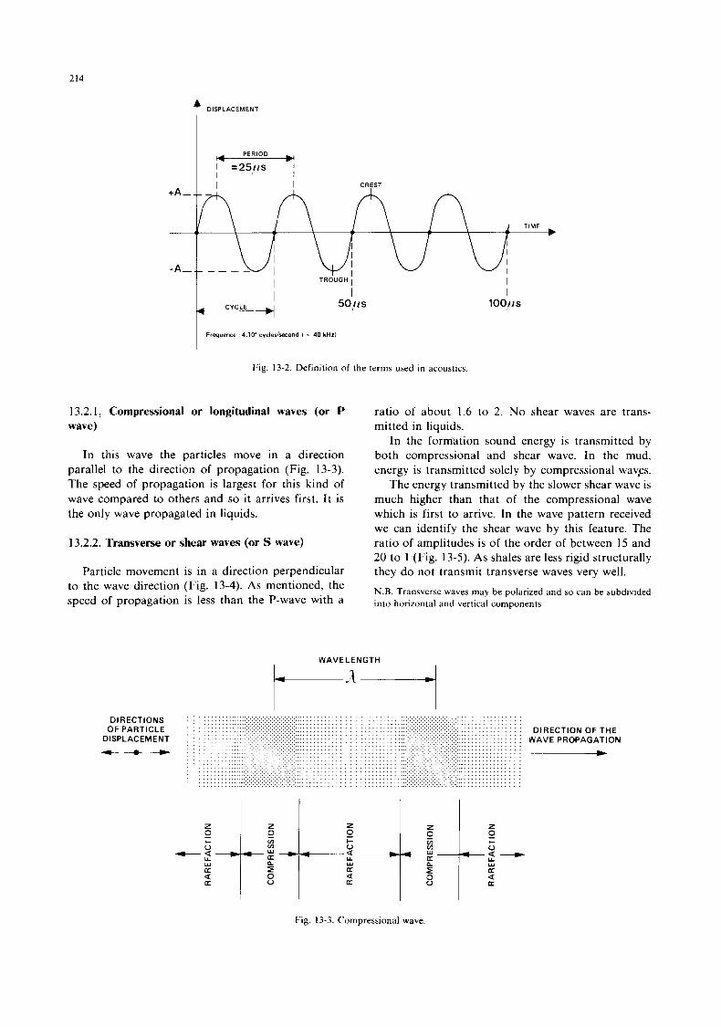
214
? DISPLACEMENT
PERIOD
I =25,iis I I I
I 50,irs
I 100,~s
I Frequence 4 10' cyclerlrecond ( ~ 40 kHz)
Fig. 13-2. Definition of the terms used in acoustics.
13.2.1 : Compressional or longitudinal waves (or P wave)
In this wave the particles move in a direction parallel to the direction of propagation (Fig. 13-3). The speed of propagation is largest for this kind of wave compared to others and so it arrives first. It is the only wave propagated in liquids.
13.2.2. Transverse or shear waves (or S wave)
Particle movement is in a direction perpendicular to the wave direction (Fig. 13-4). As mentioned, the speed of propagation is less than the P-wave with a
ratio of about 1.6 to 2. No shear waves are trans- mitted in liquids.
In the form'ation sound energy is transmitted by both compressional and shear wave. In the mud, energy is transmitted solely by compressional wav,es.
The energy transmitted by the slower shear wave is much higher than that of the compressional wave which is first to arrive. In the wave pattern received we can identify the shear wave by this feature. The ratio of amplitudes is of the order of between 15 and 20 to 1 (Fig. 13-5). As shales are less rigid structurally they do not transmit transverse waves very well. N.B. Transverse waves may he polarized and so can he subdivided into horizontal and vertical components
WAVELENGTH
I DIRECTIONS
OF PARTICLE DISPLACEMENT --
z 0 + V - 2 4 w a U a
. . . . . . . . . . . . . . ..................
2 0 I- V 6 2 - Y a
a U
: DIRECTION OF THE : WAVE PROPAGATION
:-
Fig. 13-3. Compressional wave.
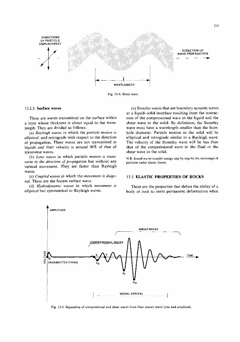
215
D ISPLACEMENT
a i l + W A V E L E N G T H
Fig. 13-4. Shear wave.
13.2.3. Surface waves
These are waves transmitted on the surface within a layer whose thickness is about equal to the wave- length. They are divided as follows:
(a) Rayleigh waves in which the particle motion is elliptical, and retrograde with respect to the direction of propagation. These waves are not transmitted in liquids and their velocity is around 90% of that of transverse waves.
(b) Love waves in which particle motion is trans- verse to the direction of propagation but without any vertical movement. They are faster than Rayleigh waves.
(c) Coupled waves in which the movement is diago- nal. These are the fastest surface wave.
(d) Hydrodynamic waves in which movement is elliptical but symmetrical to Rayleigh waves.
AMPLITUDE 1
(e) Stoneley waves that are boundary acoustic waves at a liquid-solid interface resulting from the interac- tion of the compressional wave in the liquid and the shear wave in the solid. By definition, the Stoneley wave must have a wavelength smaller than the bore- hole diameter. Particle motion in the solid will be elliptical and retrograde similar to a Rayleigh wave. The velocity of the Stoneley wave will be less than that of the compressional wave in the fluid or the shear wave in the solid. N.B. Sound waves transfer energy step by step by the movemept of particles under elastic forces.
13.3. ELASTIC PROPERTIES OF ROCKS
These are the properties that define the ability of a body or rock to resist permanent deformation when
SHEAR WAVES
I SIGNAL ARRIVAL
Fig. 13-5. Separation of compressional and shear waves from their transit travel time and amplitude.
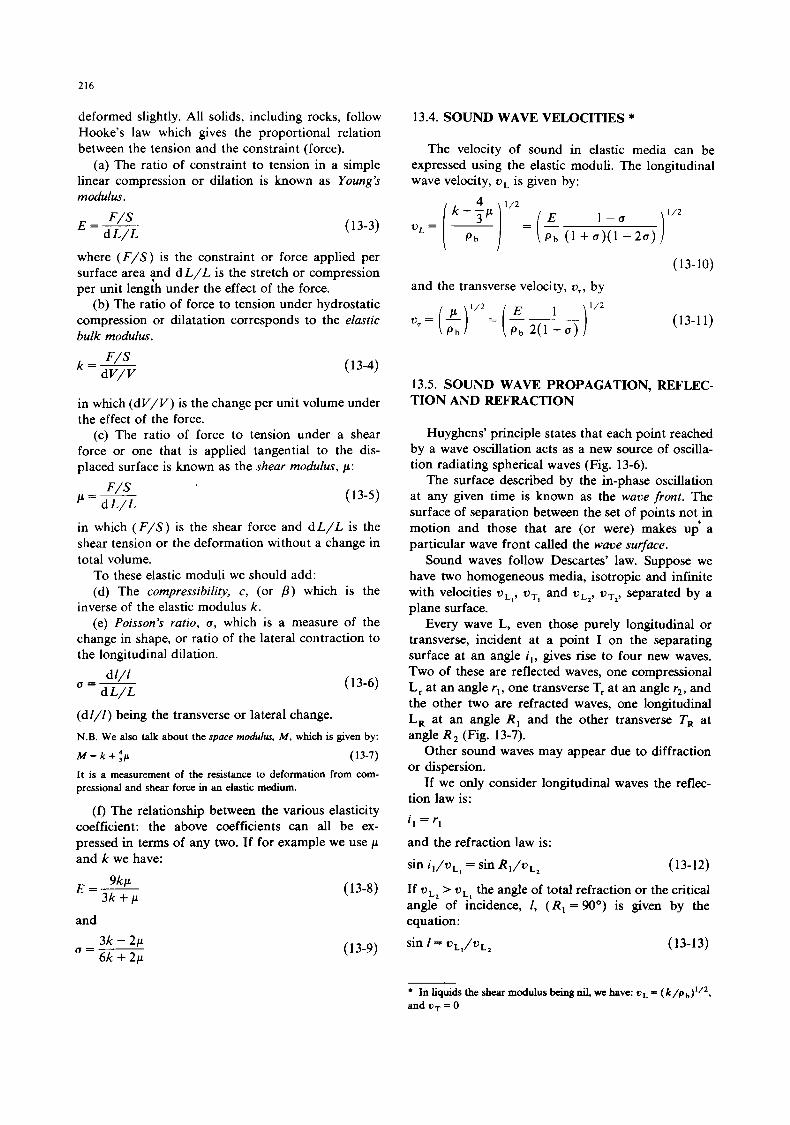
216
deformed slightly. All solids, including rocks, follow Hooke's law which gives the proportional relation between the tension and the constraint (force).
(a) The ratio of constraint to tension in a simple linear compression or dilation is known as Young's modulus.
(13-3)
where ( F / S ) is the constraint or force applied per surface area ?nd dL/L is the stretch or compression per unit length under the effect of the force.
(b) The ratio of force to tension under hydrostatic compression or dilatation corresponds to the elastic bulk modulus.
(1 3-4)
in which (dV/V) is the change per unit volume under the effect of the force.
(c) The ratio of force to tension under a shear force or one that is applied tangential to the dis- placed surface is known as the shear modulus, p:
( 13-5)
in which ( F / S ) is the shear force and d L/L is the shear tension or the deformation without a change in total volume.
To these elastic moduli we should add: (d) The compressibility, c, (or p ) which is the
inverse of the elastic modulus k. (e) Poisson's ratio, (I, which is a measure of the
change in shape, or ratio of the lateral contraction to the longitudinal dilation.
d 1/1 d L/L
o=- ( 13-6)
(d I / I ) being the transverse or lateral change. N.B. We also talk about the space modulus, M , which is given by:
M = k + ! p ( 13-7)
I t is a measurement of the resistance to deformation from com- pressional and shear force in an elastic medium.
(f) The relationship between the various elasticity coefficient: the above coefficients can all be ex- pressed in terms of any two. If for example we use p and k we have:
E = - 9kP 3 k + p
and 3k - 2 p
(J=-
6k + 2 p
( 13-8)
(1 3-9)
13.4. SOUND WAVE VELOCITIES *
The velocity of sound in elastic media can be expressed using the elastic moduli. The longitudinal wave velocity, v L is given by:
~~
J = ( ~ h ( l + o ) ( 1 - 2 u ) J (13-10)
and the transverse velocity, vT, by
(13-1 1)
13.5. SOUND WAVE PROPAGATION, REFLEC- TION AND REFRACTION
Huyghens' principle states that each point reached by a wave oscillation acts as a new source of oscilla- tion radiating spherical waves (Fig. 13-6).
The surface described by the in-phase oscillation at any given time is known as the wave front. The surface of separation between the set of points not in motion and those that are (or were) makes u$ a particular wave front called the wave surface.
Sound waves follow Descartes' law. Suppose we have two homogeneous media, isotropic and infinite with velocities vLl , vT, and uL2, vT2, separated by a plane surface.
Every wave L, even those purely longitudinal or transverse, incident at a point I on the separating surface at an angle z, , gives rise to four new waves. Two of these are reflected waves, one compressional L, at an angle r , , one transverse T, at an angle r,, and the other two are refracted waves, one longitudinal L, at an angle R, and the other transverse TR at angle R, (Fig. 13-7).
Other sound waves may appear due to diffraction or dispersion.
If we only consider longitudinal waves the reflec- tion law is: i , = r,
and the refraction law is: sin i , / v L l = sin R 1 / v L 2 (13-12)
If vL, > v the angle of total refraction or the critical angle of mcidence, I, ( R , = 90") is given by the equation: sin I = uL,/uL2 (13-13)
41
* In liquids the shear modulus being nil, we have: wL = ( k / p b ) ' I 2 , andwT=O
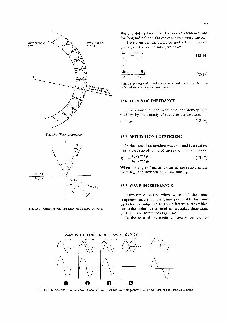
217
WAVE FRONT AT WAVE FRONT AT
/
I VI
Fig. 13-6. Wave propagation.
Fig. 13-7. Reflection and refraction of an acoustic wave.
We can define two critical angles of incidence, one for longitudinal and the other for transverse waves.
If we consider the reflected and refracted waves given by a transverse wave, we have: sin i, sin r, (13-14) -=-
v L , T,
and sin i, sin R,
OLI " T2 - (!3-15)
N.B. In the case of a wellbore where medium 1 is a fluid the reflected transverse wave does not exist.
13.6. ACOUSTIC IMPEDANCE
This is given by the product of the density of a medium by the velocity of sound in the medium: r = "IPI (13-16)
13.7. REFLECTION COEFFICIENT
In the case of an incident wave normal to a surface this is the ratio of reflected energy to incident energy:
(13-17)
When the angle of incidence varies, the ratio changes from R1-, and depends on i,, .vT, and vT,.
V2P2 - V I P 1
V2P2 + U l P l RI-2 =
13.8. WAVE INTERFERENCE
Interference occurs when waves of the same frequency arrive at the same point. At this time particles are subjected to two different forces which can either reinforce or tend to neutralise depending on the phase difference (Fig. 13-8).
In the case of the sonic, emitted waves are re-
WAVE INTERFERENCE AT THE SAME FREQUENCY
0 0 0 0 Fig. 13-8. Interference phenomenon of acoustic waves of the same frequency I , 2, 3 and 4 are of the same wavelength.

218
flected or refracted at the borehole wall. However, as this is not perfectly cylindrical and the tool axis is rarely at the hole axis, wave interference may occur.
13.9. REFERENCES
See end of chapter 14.
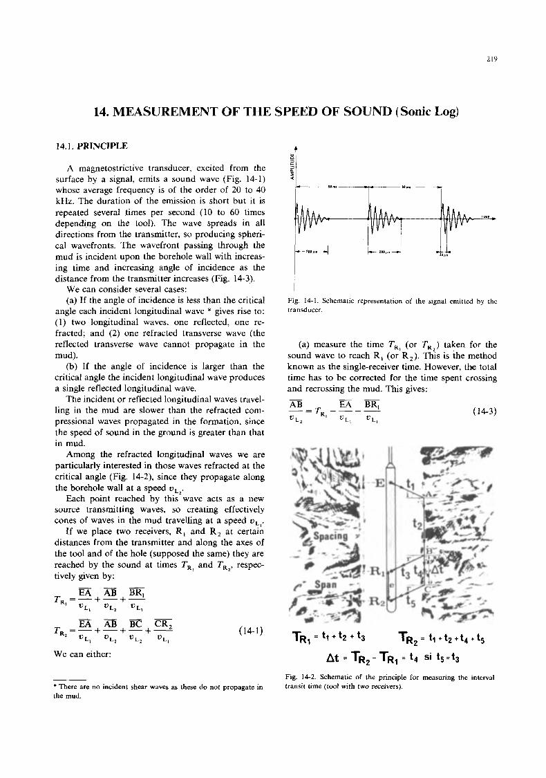
219
14. MEASUREMENT OF THE SPEED OF SOUND (Sonic Log)
14.1. PRINCIPLE
A magnetostrictive transducer, excited from the surface by a signal, emits a sound wave (Fig. 14-1) whose average frequency is of the order of 20 to 40 kHz. The duration of the emission is short but it is repeated several times per second (10 to 60 times depending on the tool). The wave spreads in all directions from the transmitter, so producing spheri- cal wavefronts. The wavefront passing through the mud is incident upon the borehole wall with increas- ing time and increasing angle of incidence as the distance from the transmitter increases (Fig. 14-3).
We can consider several cases: (a) If the angle of incidence is less than the critical
angle each incident longitudinal wave * gives rise to: (1) two longitudinal waves, one reflected, one re- fracted; and (2) one refracted transverse wave (the reflected transverse wave cannot propagate in the mud).
(b) If the angle of incidence is larger than the critical angle the incident longitudinal wave produces a single reflected longitudinal wave.
The incident or reflected longitudinal waves travel- ling in the mud are slower than the refracted com- pressional waves propagated in the formation, since the speed of sound in the ground is greater than that in mud.
Among the refracted longitudinal waves we are particularly interested in those waves refracted at the critical angle (Fig. 14-2), since they propagate along the borehole wall at a speed v L , .
Each point reached by this wave acts as a new source transmitting waves, so creating effectively cones of waves in the mud travelling at a speed uL,.
If we place two receivers, R, and R, at certain distances from the transmitter and along the axes of the tool and of the hole (supposed the same) they are reached by the sound at times TRl and TR,, respec- tively given by: - E A A B B R ,
TR, =- + - + - V L , VL, V L ,
E A A B B C C R V L , VL, V L , V L ,
T =-+-+++2
We can either:
R2 (14-1)
* There are no incident shear waves as these do not propagate in the mud.
c
Fig. 14-1. Schematic representation of the signal emitted by the transducer.
(a) measure the time TR, (or TR2) taken for the sound wave to reach R , (or R,). This is the method known as the single-receiver time. However, the total time has to be corrected for the time spent crossing and recrossing the mud. This gives:
(14-3)
- -E
Fig. 14-2. Schematic of the principle for measuring the interval transit time (tool with two receivers).
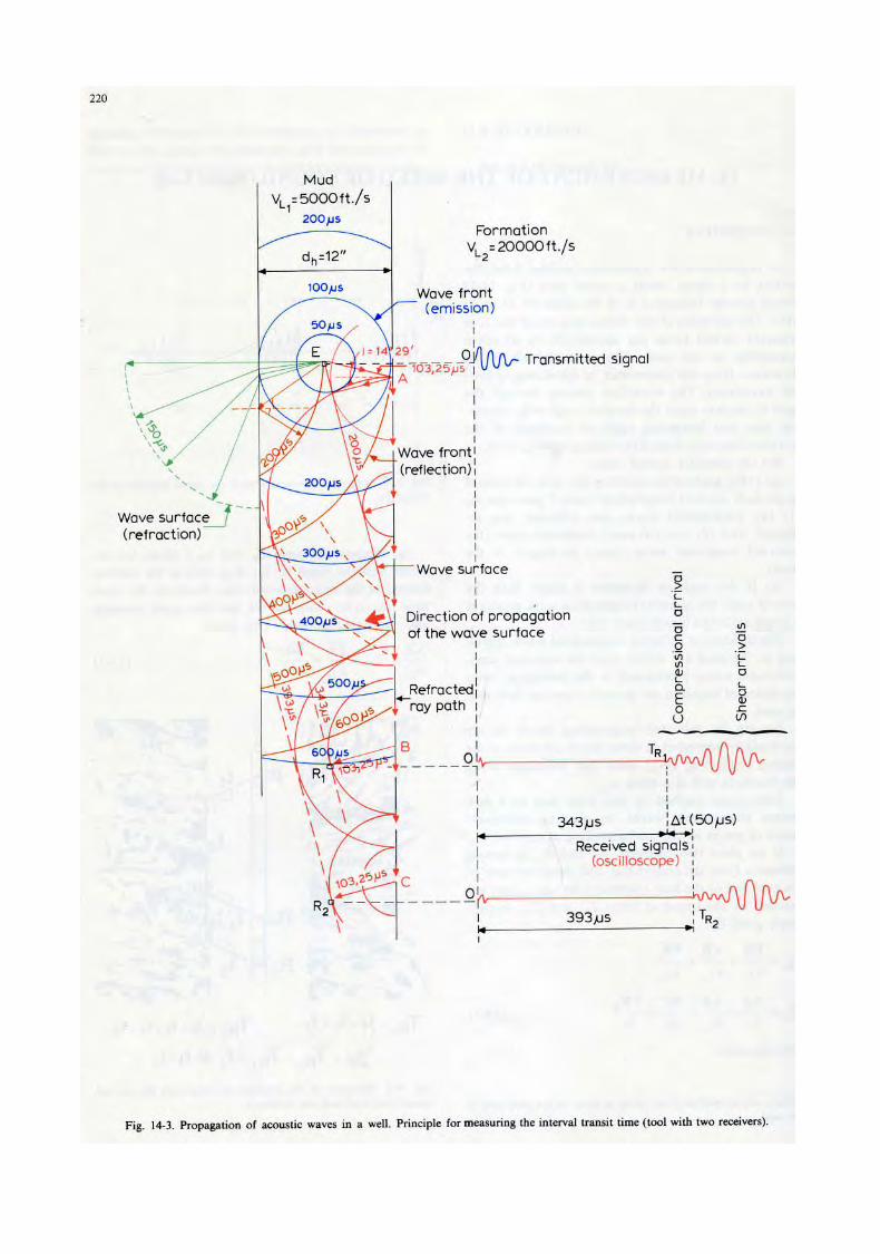
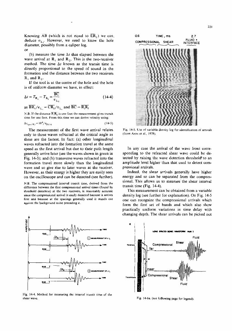
22 I
Knowing AB (which is not equal to m,) we can. 0.6 TIME, ms 2.7 deduce uL,. However, we need to know the hole diameter, possibly from a caliper log. or
(b) measure the time A t that elapsed between the wave arrival at R, and R,. This is the two-receiver method. The time At known as the transit time is directly proportional to the speed of sound in the formation and the distance between the two receivers R , and R,.
If the tool is at the centre of the hole and the hole is of uniform diameter we have, in effect:
- ( 14-4)
BC
vL,
A t = T - T =- R, Rl
- - as m / v L I = =/uLI and BC = R,Rz N.B. If the distance time for one foot. From this time we can derive velocity using:
*&,f,) = 106/%,,) (14-5)
is one foot the measurement gives transit
The measurement of the first wave arrival relates only to those waves refracted at the critical angle as these are the fastest. In fact: (a) other lonjytudinal waves refracted into the formation travel at the same speed as the first arrival but due to their path length generally arrive later (see the waves shown in green in Fig. 14-3); and (b) transverse waves refracted into the formation travel more slowly than the longitudinal wave and so give rise to later waves at the receiver. However, as their energy is higher they are easily seen on the oscilloscope and can be detected (see further). N.B. The compressional interval transit time, derived from the difference between the first compressional arrival times (found by threshold detection) at the two receivers, is reasonably accurate since the compressional arrival is easily detected because it arrives first and because at the spacings generally used it stands out against the background noise preceding it.
'I *TIME
IIM k
9 * 1ME 0-
@ MEIIUREMENT OF &I,
'I I *TIME
0 9
Fig. 14-4. Method for measuring the interval transit time of the shear wave.
Fig. 14-5. Use of variable density log for identification of arrivals (from Aron et al., 1978).
In any case the arrival of the wave front corre- sponding to the refracted shear wave could be de- tected by raising the wave detection threshold' to an amplitude level higher than that used to detect com- pressional arrivals.
Indeed, the shear arrivals generally have higher energy and so can be separated from the compres- sional. This allows us to measure' the shear interval transit time (Fig. 14-4).
This measurement can be obtained from a variable density log (see further for explanation). On Fig. 14-5 one can recognize the compressional arrivals which form the first set of bands and which also show practically uniform variations in time delay with changing depth. The shear arrivals can be picked out
I I Fluid
Fig. 14-6a. (see following page for legend).
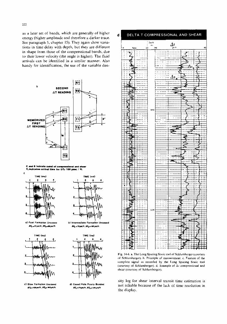
222
AT SECOND READING
as a later set of bands, which are generally of higher energy (higher amplitude and therefore a darker trace. See paragraph 5, chapter 15). They again show varia- tions in time delay with depth, but they are different in shape from those of the compressional bands, due to their lower velocity (the angle is higher). The fluid arrivals can be identified in a similar manner. Also handy for identification, the use of the variable den-
@I%h 3--.,
b
MEMORIZED
a
U
C and S Indlcata onaot of conproaolonal and mhur F. Indlcatoa arrival tlma for DT- 189 poc / ft.
C
TIME (ma)
1 2 3 4
a) Fast Formation Uncasea
A%- 5~p/ft,ATs=.6psfh
TIME (ms) 1 2 3 4
C S F
c ) Slow Forrnatlon Uncaied AT.=msrflt, A s - MJwltt
TIME (ma) 1 2 3 4 C S F
b) Intermediate Formation Uncased A~=IZ(rfft .ATs=UOplh
TIME (mi) 1 2 3 4 5 C S F
I
dl Cased Hole Poorly Bonded ATc =75pfft. ATs -?2s pail1
Fig. 14-6. a. The Long Spacing Sonic tool of Schlumberger (courtesy of Schlumberger). b. Principle of measurement. c. Feature of the complete signal as recorded by the Long Spacing Sonic tool (courtesy of Schlumberger). d. Example of A t compressional and shear (courtesy of Schlumberger).
sity log for shear interval transit time estimation is not reliable because of the lack of time resolution in the display.
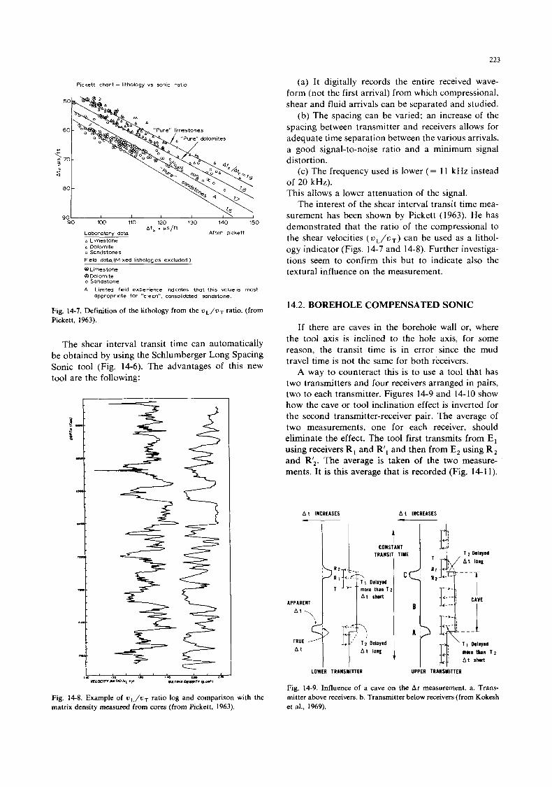
223
Pickett chart - lithology vs sonic rat io
50
60
c
5 70 4
z 80
\\ 90 I I I 4 I
90 100 110 120 130 140 150 Ats . p / f t
Laboratory data After pichett
A Limestone A Dolomite a Sandstones Field data(Mined litholoaies excluded
@Limestone @Dolomite o Sandstone
A Limrted field experience indicates that this value is most appropriate for "clean", consolidcrled sandstone
Fig. 14-7. Definition of the lithology from the uL/uT ratio. (from Pickett, 1963).
The shear interval transit time can automatically be obtained by using the Schlumberger Long Spacing Sonic tool (Fig. 14-6). The advantages of this new tool are the following:
? m 1 0 ..* L.D 270
VfLoEIN RA?WI.p.lr 1I"T"I.X m r v h.&l 8 -
Fig. 14-8. Example of uL/uT ratio log and comparison with the matrix density measured from cores (from Pickett, 1963).
(a) It digitally records the entire received wave- form (not the first arrival) from which compressional, shear and fluid arrivals can be separated and studied.
(b) The spacing can be varied; an increase of the spacing between transmitter and receivers allows for adequate time separation between the various arrivals, a good signal-to-noise ratio and a minimum signal distortion.
(c) The frequency used is lower ( = 11 kHz instead of 20 kHz). This allows a lower attenuation of the signal.
The interest of the shear interval transit time mea- surement has been shown by Pickett (1963). He has demonstrated that the ratio of the compressional to the shear velocities (oL/uT) can be used as a lithol- ogy indicator (Figs. 14-7 and 14-8). Further investiga- tions seem to confirm this but to indicate also the textural influence on the measurement.
14.2. BOREHOLE COMPENSATED SONIC
If there are caves in the borehole wall or, where the tool axis is inclined to the hole axis, for some reason, the transit time is in error since the mud travel time is not the same for both receivers.
A way to counteract this is to use a tool that has two transmitters and four receivers arranged in pairs, two to each transmitter. Figures 14-9 and 14-10 show how the cave or tool inclination effect is inverted for the second transmitter-receiver pair. The average of two measurements, one for each receiver, should eliminate the effect. The tool first transmits from E, using receivers R, and R', and then from E, using R, and R;. The average is taken of the two measure- ments. It is this average that is recorded (Fig. 14-1 1).
A t INCREASES A t INCREASES 4 I
t 1 1 CONSTANl I TRANSIT
more than T z A t short
'' 1 2 Delayed A t long
r
TIME
CC
B
A
LOWER TRANSMITTER UPPER TRANSMITTER
Fig. 14-9. Influence of a cave on the A r measurement. a. Trans- mitter above receivers. b. Transmitter below receivers (from Kokesh et al., 1969).
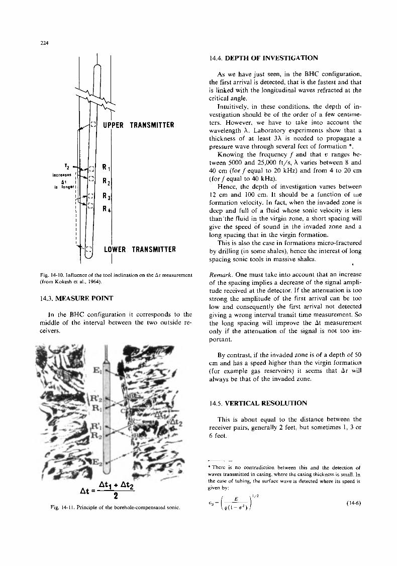
224
14.4. DEPTH OF INVESTIGATION
T2 - increases '
I A t I
is longer1 I I I I I I I I I I I I
33. TRANSMITTER
TRANSMITTER
Fig. 14-10. Influence of the tool inclination on the A t measurement (from Kokesh et al., 1964).
14.3. MEASURE POINT
In the BHC configuration it corresponds to the middle of the interval between the two outside re- ceivers.
At, + At2
2 At =
Fig. 14- I 1. Principle of the borehole-compensated sonic.
As we have just seen, in the BHC configuration, the first arrival is detected, that is the fastest and that is linked with the longitudinal waves refracted at the critical angle.
Intuitively, in these conditions, the depth of in- vestigation should be of the order of a few centime- ters. However, we have to take into account the wavelength A. Laboratory experiments show that a thickness of at least 3A is needed to propagate a pressure wave through several feet of formation *.
Knowing the frequency f and that v range? he- tween 5000 and 25,000 ft/s, A varies between 8 and 40 cm (for f equal to 20 kHz) and from 4 to 20 cm (for f equal to 40 kHz).
Hence, the depth of investigation varies between 12 cm and 100 cm. It should be a function of me formation velocity. In fact, when the invaded zone is deep and full of a fluid whose sonic velocity is less than'the fluid in the virgin zone, a short spacing will give the speed of sound in the invaded zone and a long spacing that in the virgin formation.
This is also the case in formations micro-fractured by drilling (in some shales), hence the interest of long spacing sonic tools in massive shales.
Remark. One must take into account that an increase of the spacing implies a decrease of the signal ampli- tude received at the detector. If the attenuation is too strong the amplitude of the first arrival can be too low and consequently the first arrival not detected giving a wrong interval transit time measurement. So the long spacing will improve the At measurement only if the attenuation of the signal is not too im- portant.
.
By contrast, if the invaded zone is of a depth of 50 cm and has a speed higher than the virgin formation (for example gas reservoirs) it seems that A t will always be that of the invaded zone.
14.5. VERTICAL RESOLUTION
This is about equal to the distance between the receiver pairs, generally 2 feet, but sometimes 1, 3 or 6 feet.
*There is no contradiction between this and the detection of waves transmitted in casing, where the casing thickness is small. In the case of tubing, the surface wave is detected where its speed is given by:
( 14-6)
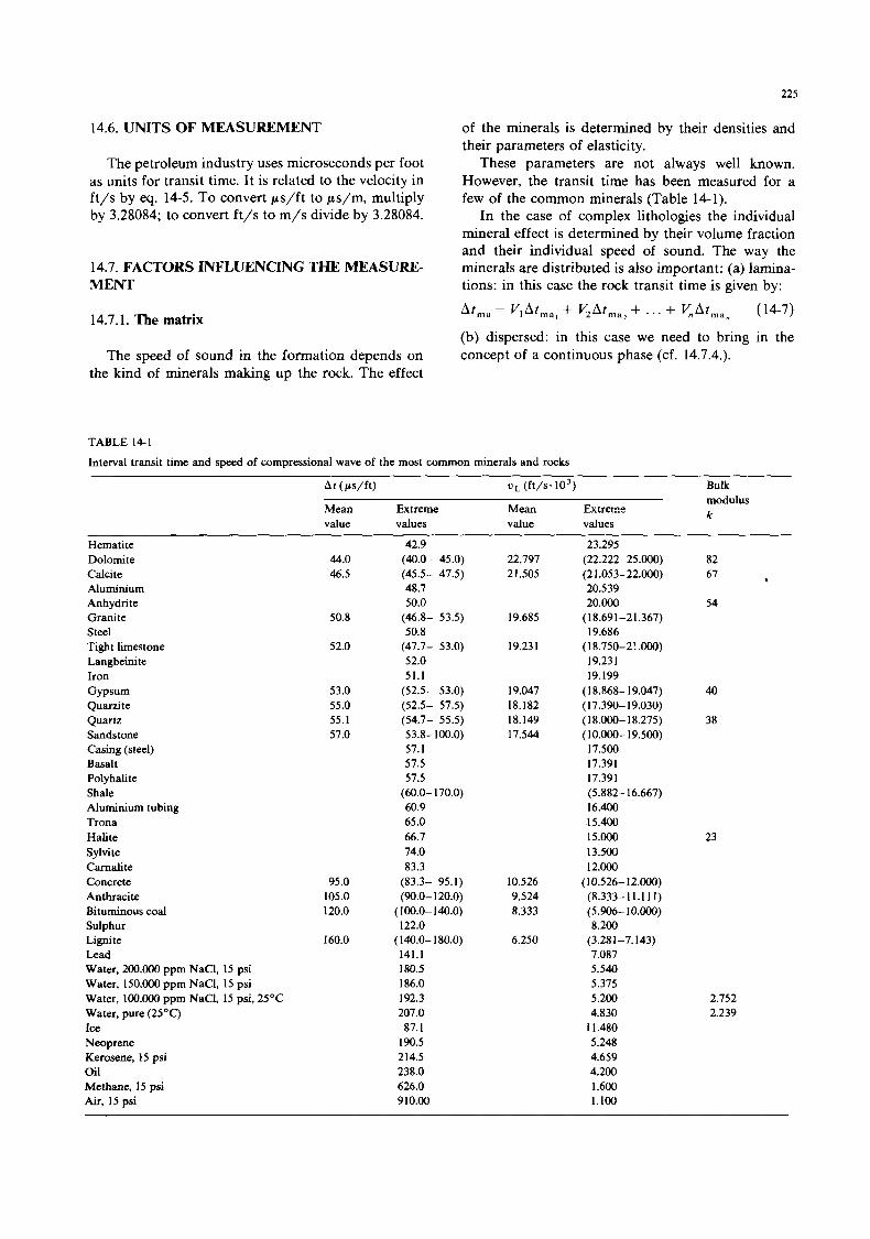
225
14.6. UNITS OF MEASUREMENT
The petroleum industry uses microseconds per foot as units for transit time. It is related to the velocity in ft/s by eq. 14-5. To convert ps/ft to ps/m, multiply by 3.28084; to convert ft/s to m/s divide by 3.28084.
14.7. FACTORS INFLUENCING THE MEASURE- MENT
14.7.1. The matrix
The speed of sound in the formation depends on the kind of minerals making up the rock. The effect
of the minerals is determined by their densities and their parameters of elasticity.
These parameters are not always well known. However, the transit time has been measured for a few of the common minerals (Table 14-1).
In the case of complex lithologies the individual mineral effect is determined by their volume fraction and their individual speed of sound. The way the minerals are distributed is also important: (a) lamina- tions: in this case the rock transit time is given by: At,, = V,Atma, + VZAtma2 + . . . + VHAtman (14-7)
(b) dispersed: in this case we need to bring in the concept of a continuous phase (cf. 14.7.4.).
TABLE 14-1
Interval transit time and speed of compressional wave of the most common minerals and rocks
A t (as/ft) DL (ft/s. lo3) Bulk
Mean Extreme Mean Extrecs value values value values
modulus k
Hematite Dolomite Calcite Aluminium Anhydrite Granite Steel Tight limestone Langbeinite Iron Gypsum Quarzite Quartz Sandstone Casing (steel) Basalt Polyhalite Shale Aluminium tubing Trona Halite Sylvite Carnalite Concrete Anthracite Bituminous coal Sulphur Lignite Lead Water, 200.000 ppm NaCI, I5 psi Water, 150.000 ppm NaCI, 15 psi Water, 100.000 ppm NaCI, 15 psi, 25°C Water, pure (25°C) Ice Neoprene Kerosene, 15 psi oi l Methane, 15 psi Air, 15 psi
44.0 46.5
50.8
52.0
53.0 55.0 55.1 57.0
95.0 105.0 120.0
160.0
42.9 (40.0- 45.0)
48.7 50.0
50.8
52.0 51.1
(45.5- 47.5)
(46.8- 53.5)
(47.7- 53.0)
(52.5- 53.0) (52.5- 57.5)
53.8-100.0) 57.1 57.5 57.5
(60.0-170.0) 60.9 65.0 66.7 74.0 83.3
(54.7- 55.5)
(83.3- 95.1) (90.0- 120.0)
(100.0- 140.0) 122.0
141.1 180.5 186.0 192.3 207.0 87.1
190.5 214.5 238.0 626.0 910.00
( 140.0- 180.0)
22.797 21.505
19.685
19.231
19.047 18.182 18.149 17.544
10.526 9.524 8.333
6.250
23.295 (22.222-25.000) 82 (21.053-22.000) 67 20.539 20.000 54
19.686
19.231 19.199
*
(18.691-21.367)
(18.750-21 .000)
(18.868- 19.047) 40 (17.390-19.030) ( 18.000- 18.275) 38 (10.000-19.500) 17.500 17.391 17.391
16.400 15.400 15.000 13.500 12.000
(10.526-12.000) (8.333-11.111)
(5.882- 16.667)
(5.906- 10.000) 8.200
(3.281-7.143) 7.087 5.540 5.375 5.200 4.830
1 1.480 5.248 4.659 4.200 1.600 1.100
23
2.752 2.239
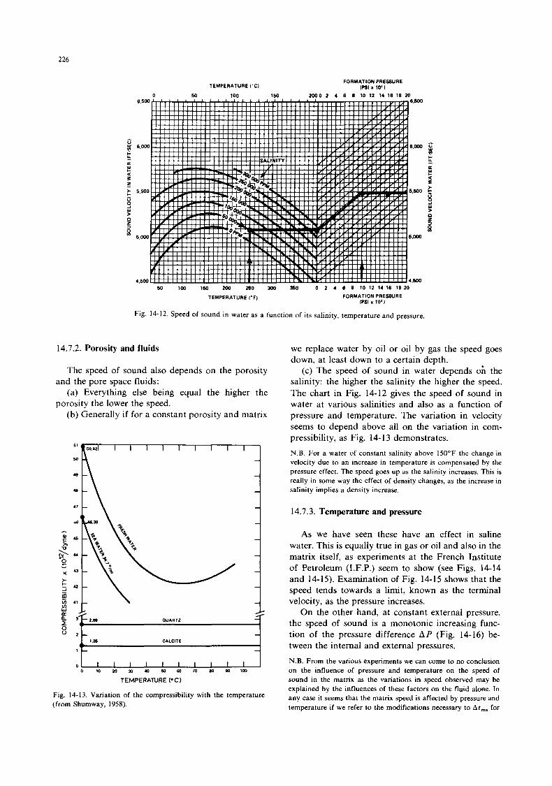
226
- 0
s c U Y
5
$ L t >
> 0
3 w
Fig. 14-12. Speed of sound in water as a function of its salinity, temperature and pressure.
14.7.2. Porosity and fluids
The speed of sound also depends on the porosity
(a) Everything else being equal the higher the
(b) Generally if for a constant porosity and matrix
and the pore space fluids:
porosity the lower the speed.
CALCITE :: a ia m a aa so 60 10 BO 90 im
TEMPERATURE ( 'C)
Fig. 14-13. Variation of the compressibility with the temperature (from Shumway, 1958).
we replace water by oil or oil by gas the speed goes down, at least down to a certain depth.
(c) The speed of sound in water depends oh the salinity: the higher the salinity the higher the speed. The chart in Fig. 14-12 gives the speed of sound in water at various salinities and also as a function of pressure and temperature. The variation in velocity seems to depend above all on the variation in com- pressibility, as Fig. 14- 13 demonstrates. N.B. For a water of constant salinity above 150°F the change in velocity due to an increase in temperature is compensated by the pressure effect. The speed goes up as the salinity increases. This is really in some way the effect of density changes, as the increase in salinity implies a density increase.
1 4.7.3. Temperature and pressure
As we have seen these have an effect in saline water. Ths is equally true in gas or oil and also in the matrix itself, as experiments at the French Institute of Petroleum (I.F.P.) seem to show (see Figs. 14-14 and 14-15). Examination of Fig. 14-15 shows that the speed tends towards a limit, known as the terminal velocity, as the pressure increases.
On the other hand, at constant external pressure, the speed of sound is a monotonic increasing func- tion of the pressure difference A P (Fig. 14-16) be- tween the internal and external pressures. N.B. From the various experiments we can come to no conclusion on the influence of pressure and temperature on the speed of sound in the matrix as the variations in speed observed may be explained by the influences of these factors on the fluid alone. In any case it seems that the matrix speed is affected by pressure and temperature if we refer to the modifications necessary to At,, for
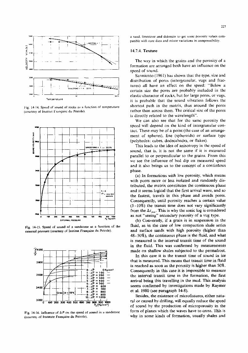
227
5 > 4 9 m
I 1
1 1 I
Fig. 14-14. Speed of sound of rocks as a function of temperature (courtesy of Institut FranGaise du Petrole).
Fig. 14-15. Speed of sound of a sandstone as a function of the external pressure (courtesy of Institut Franpise du Petrole).
- t4000 E u
3800
3 600
3400
3 200 0 100 200 300 400 500 600 700 800 900 lo00
PE (Kglcm’)
Fig. 14-16. Influence of A P on the speed of sound in a sandstone (courtesy of Institute Franpise du Petrole).
a sand, limestone and dolomite to get sonic porosity values com- patible with core data and minor variations in compressibility.
14.7.4. Texture
The way in which the grains and the porosity of a formation are arranged both have an influence on the speed of sound.
Sarmiento (1961) has shown that the type, size and distribution of pores (intergranular, vugs and frac- tures) all have an effect on the speed: “Below a certain size the pores are probably included in the elastic character of rocks, but for large pores, or vugs, it is probable that the sound vibration follows the shortest path in the matrix, thus around the pores rather than across them. The critical size of the pores is directly related to the wavelength”.
We can also see that for the same porosity the speed will depend on the kind of intergranular con- tact. These may be of a point (the case of an arrange- ment of spheres), line (spheroids) or surface type (polyhedra: cubes, dodecahedra, or flakes).
This leads to the idea of anisotropy in the speed of sound, that is, it is not the same if it is measured parallel to or perpendicular to the grains. From this we see the influence of bed dip on measured speed and it also brings us to the concept of a continhous phase.
(a) In formations with low porosity, which means with pores more or less isolated and randomly dis- tributed, the matrix constitutes the continuous phase and it seems logical that the first arrival wave, and so the fastest, travels in t h s phase and avoids pores. Consequently, until porosity reaches a certain value (5- 10%) the transit time does not vary significantly from the Atma. This is why the sonic log is considered as not “seeing” secondary porosity of a vug type.
(b) Conversely, if a grain is in suspension in the fluid, as in the case of low compaction shale series and surface sands with high porosity (higher than 48-50%), the continuous phase is the fluid, and what is measured is the interval transit time of the sound in the fluid. This was confirmed by measurements made on shallow shales subjected to the permafrost.
In this case it is the transit time of sound in ice that is measured. This means that transit time in fluid is reached as soon as the porosity is higher than 50%. Consequently in this case it is impossible to measure the interval transit time in the formation, the first amval being this travelling in the mud. This analysis seems confirmed by investigations made by Raymer et al. 1980 (see paragraph 14-8).
Besides, the existence of microfissures, either natu- ral or caused by drilling, will equally reduce the speed of sound by the production of microporosity in the form of planes which the waves have to cross. This is why in some kinds of formation, usually shales and
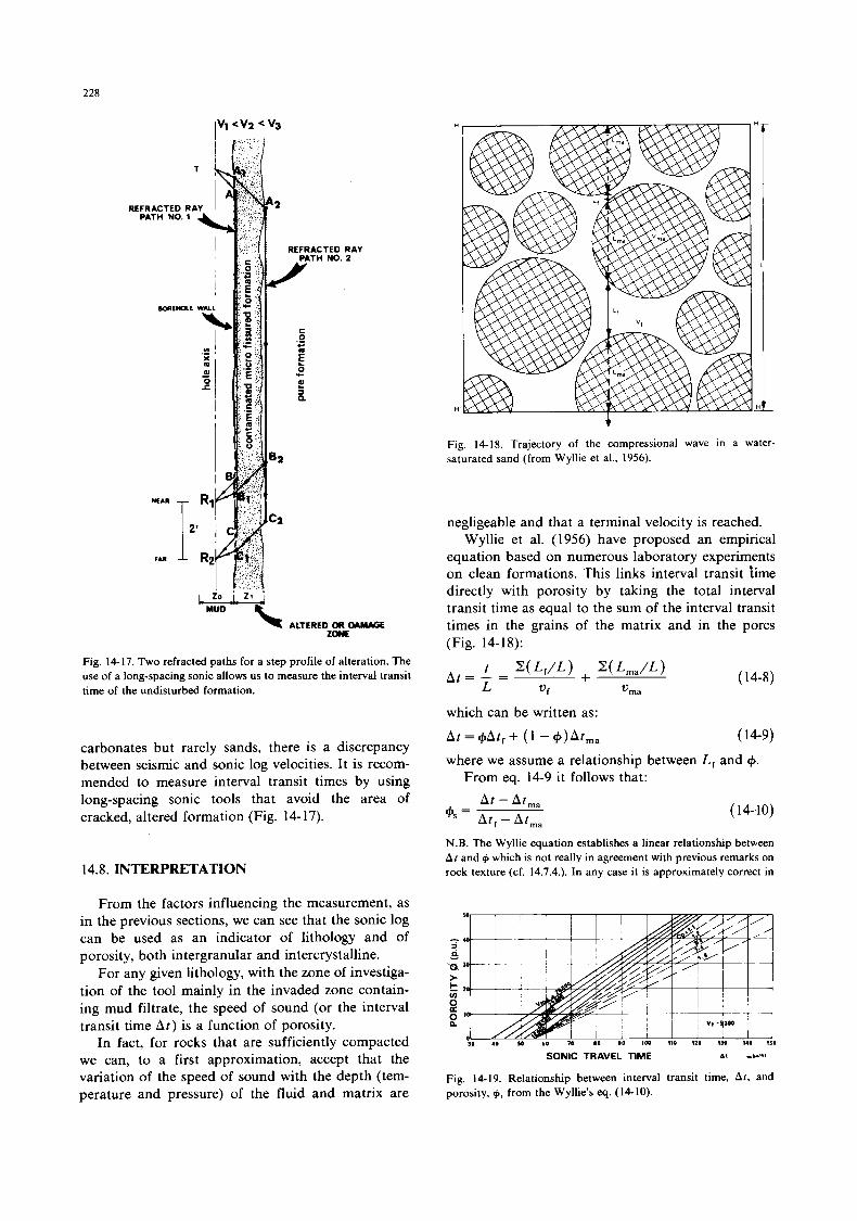
228
RAY 2
L zo i ZI i
MUD \ ALTERED OR MMMX ZONE
Fig. 14-17. Two refracted paths for a step profile of alteration. The use of a long-spacing sonic allows us to measure the interval transit time of the undisturbed formation.
carbonates but rarely sands, there is a discrepancy between seismic and sonic log velocities. It is recom- mended to measure interval transit times by using long-spacing sonic tools that avoid the area of cracked, altered formation (Fig. 14-17).
14.8. INTERPRETATION
From the factors influencing the measurement, as in the previous sections, we can see that the sonic log can be used as an indicator of lithology and of porosity, both intergranular and intercrystalline.
For any gwen lithology, with the zone of investiga- tion of the tool mainly in the invaded zone contain- ing mud filtrate, the speed of sound (or the interval transit time A t ) is a function of porosity.
In fact, for rocks that are sufficiently compacted we can, to a first approximation, accept that the variation of the speed of sound with the depth (tem- perature and pressure) of the fluid and matrix are
Fig. 14-18. Trajectory of the compressional wave in a water- saturated sand (from Wyllie et al., 1956).
negligeable and that a terminal velocity is reached. Wyllie et al. (1 956) have proposed an empirical
equation based on numerous laboratory experiments on clean formations. This links interval transit time directly with porosity by taking the total interval transit time as equal to the sum of the interval transit times in the grains of the matrix and in the pores (Fig. 14-18):
(14-8)
(14-9)
where we assume a relationship between L, and +. From eq. 14-9 it follows that:
A t - Atma
's= A t , - Atrna (14-10)
N.B. The Wyllie equation establishes a linear relationship between A r and + which is not really in agreement with previous remarks on rock texture (cf. 14.7.4.). In any case it is approximately correct in
\o 40 50 60 10 10 YO I W 190 120 1.30 140 IS0
SONIC TRAVEL TIME b l ~ W W
Fig. 14-19. Relationship between interval transit time, At , and porosity, +, from the Wyllie's eq. (14-10).
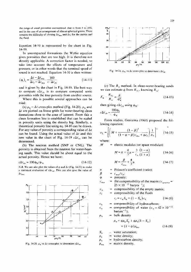
229
the range of usual porosities encountered, that is from 5 to' 25%. and in the case of an arrangement of almost spherical grains. There remains the difficulty of chosing A / m a and A / f for the matrix and the fluid.
Equation 14-10 is represented by the chart in Fig.
In uncompacted formations the Wyllie equation gives porosities that are too high. It is therefore not directly applicable. A correction factor is needed, to take into account the effects of temperature and pressure, or in other words that the terminal speed of sound is not reached. Equation 14-10 is then written:
14-19.
A t - At,, 100 .- ("')' = A t , - At,, c . Atsh
(14-1 1)
and is given by the chart in Fig. 14-19. The best way to compute c a t s h is to compare computed sonic porosities with the true porosity from another source.
Where this is possible several approaches can be tried:
(a) pb - A t cross-plot method (Fig. 14-20). pb and A t are plotted on linear grids for water-bearing clean formations close to the zone of interest. From this a clean formation line is established that can be scaled in porosity units using the density log. Similarly, a theoretical porosity line using eq. 14-10 can be drawn. For any value of porosity a corresponding value of A t can be found. Using the actual value of A t and this new value in the chart of Fig. 14-19 cAt,, can be determined.
(b) The neutron method (SNP or CNL). The porosity is obtained from the neutron for water-bear- ing sands. This value should be about equal to the actual porosity. Hence we have:
= loo%/+N (14-12) N.B. We can also plot the values of 4 and A r (Fig. 14-21) to make a statistical evaluation of cA/$,,. This can also give the value of
Alrnd.
Fig. 14-20. ph vs A / cross-plot to determine cAtS,,.
50 60 70 80 90 100 110 120 A t
P / f t
Fig. 14-21. + N vs A r cross-plot to determine C A I , ,
(c) The R , method. In clean-water-bearing sands we can estimate + from R , L , knowing R w :
then giving c a t , , using +R:
1m+, +R
c a t s h = -
(14-13)
(14-14)
From studies, Geerstma (1961) proposed the fol- lowing equation:
where: elastic modulus (or space modulus)
(14-16)
(14-17) P 4 Cm, 3
M=--+-p
Poisson's coefficient (ratio);
porosity; the compressibility of the matrix (cquart l =
25 X lo-" baryes-'); compressibility of the empty matrix; compressibility of the fluids
Cf = cwsw + (1 - S W ) C h
compressibility of hydrocarbons; compressibility of water (c, = 42 x baryes- I ) ;
bulk density
c,,/c h i
(14-18)
water saturation; water density; hydrocarbon density; matrix density.
(14-19)
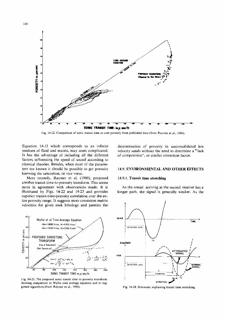
230
Fig. 14-22. Comparison of sonic transit time to core porosity from published data (from Raymer et al.. 1980).
Equation 14-15 which corresponds to an infinite medium of fluid and matrix, may seem complicated. It has the advantage of including all the different factors influencing the speed of sound according to classical theories. Besides, when most of the parame- ters are known it should be possible to get porosity knowing the saturation, or vice versa.
More recently, Raymer et al. ( 1980), proposed another transit time-to-porosity transform. This seems more in agreement with observations made. It is illustrated by Figs. 14-22 and 14-23 and provides superior transit-time-porosity correlation over the en- tire porosity range. It suggests more consistent matrix velocities for given rock lithology and permits the
100 - Wyllie et al. Time-Average Equation
(Vm=18000 I l isec. VI=5300 W s e c l
iVrn=19500 W s e c . V1=5300 I l l s e c ) 80 -
a
I I I I 1 60 80 loo 120 140 160 180 200
SONIC TRANSIT TIME-in p sec/ft
Fig. 14-23. The proposed sonic transit time to porosity transform. showing comparison to Wyllie time average equation and to sug- gested algorithms (from Raymer et al.. 1980).
determination of porosity in unconsolidated low velocity sands without the need to determine a "lack of composition", or similar correction factor.
14.9. ENVIRONMENTAL AND OTHER EFFECTS
14.9.1. Transit time stretching
As the sound arriving at the second receiver has a longer path, the signal is generally weaker. As the
t I
€ 2
Amplitude
. -. , ..I."_. L" I I i n \ SIGNAL I/ FAR
D€T€CTION L t V t l
I E2
STRETCH / Fig. 14-24. Schematic explaining transit time stretching.
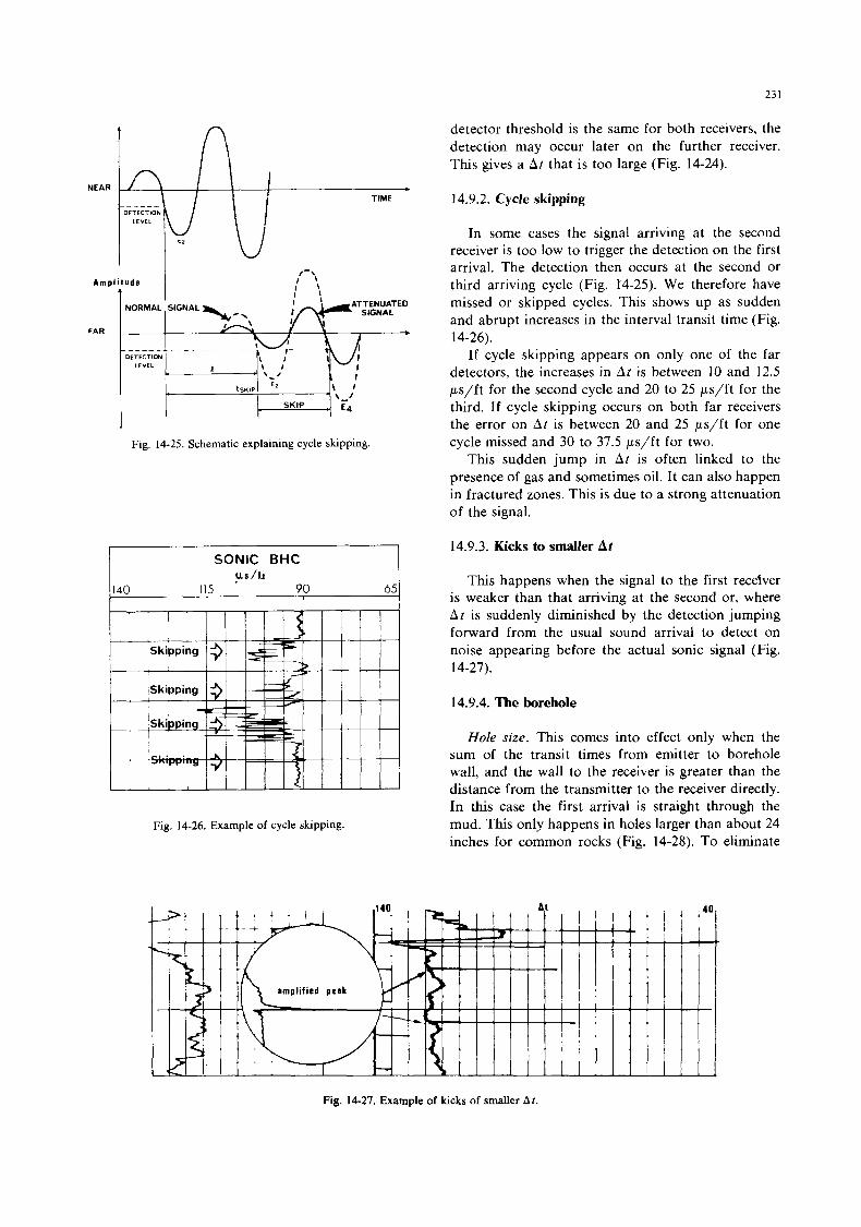
23 1
- tSKIP
i n
'-' I '* \ I
'-/ E 4 I SKIP I
Fig. 14-26, Example of cycle skipping.
detector threshold is the same for both receivers, the detection may occur later on the further receiver. This gives a A t that is too large (Fig. 14-24).
14.9.2. Cycle skipping
In some cases the signal arriving at the second receiver is too low to trigger the detection on the first arrival. The detection then occurs at the second or third arriving cycle (Fig. 14-25). We therefore have missed or skipped cycles. This shows up as sudden and abrupt increases in the interval transit time (Fig.
If cycle skipping appears on only one of the far detectors, the increases in A t is between 10 and 12.5 ps/ft for the second cycle and 20 to 25 ps/ft for the third. If cycle skipping occurs on both far receivers the error on At is between 20 and 25 ps/ft for one cycle missed and 30 to 37.5 p / f t for two.
This sudden jump in A t is often linked to the presence of gas and sometimes oil. It can also happen in fractured zones. This is due to a strong attenuation of the signal.
14-26).
14.9.3. Kicks to smaller A t
This happens when the signal to the first recelver is weaker than that arriving at the second or, where A t is suddenly diminished by the detection jumping forward from the usual sound arrival to detect on noise appearing before the actual sonic signal (Fig. 14-27).
14.9.4. The borehole
Hole size. This comes into effect only when the sum of the transit times from emitter to borehole wall, and the wall to the receiver is greater than the distance from the transmitter to the receiver directly. In t h s case the first arrival is straight through the mud. Ths only happens in holes larger than about 24 inches for common rocks (Fig. 14-28). To eliminate
Fig. 14-27. Example of kicks of smaller Ar.
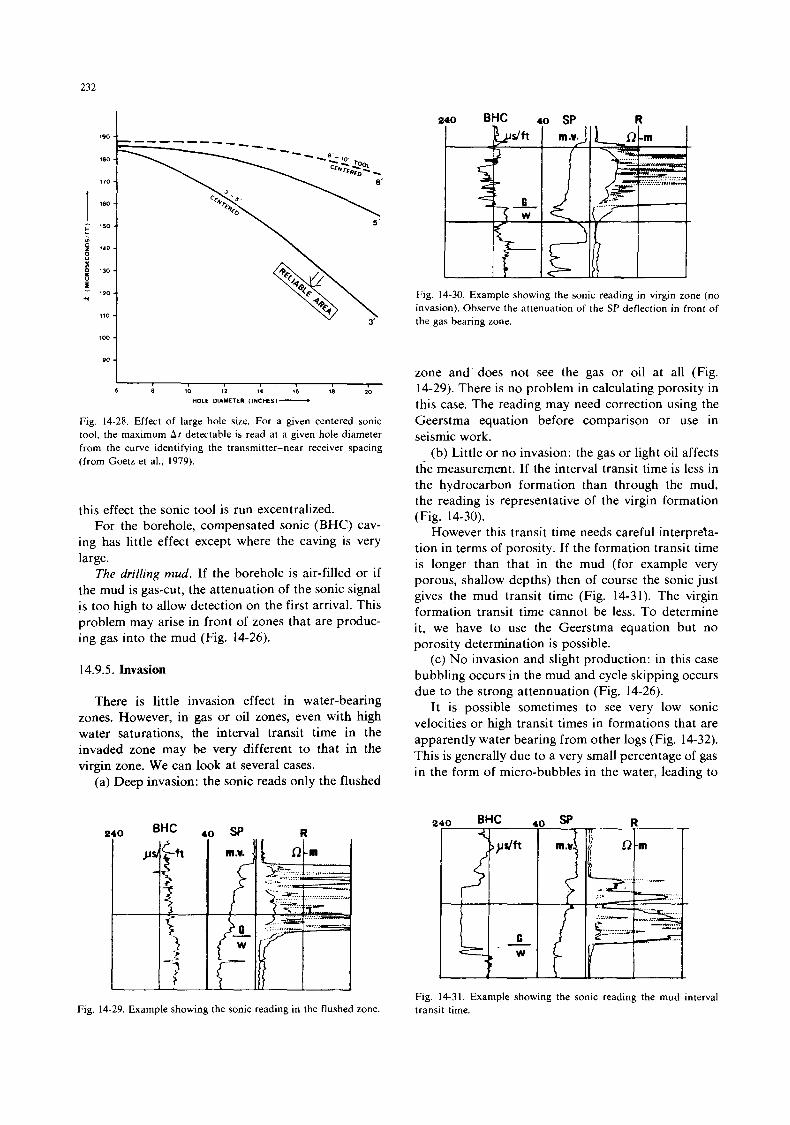
232
190
180
110
m g 140
i p 130 U
120 f Y
110
100 w l 6 8 10 12 14 16 18 20
HOLE DIAMETER (INCHES)-
Fig. 14-28. Effect of large hole size. For a given centered sonic tool, the maximum A t detectable is read at a given hole diameter from the curve identifying the transmitter-near receiver spacing (from Goetz et al.. 1979).
this effect the sonic tool is run excentralized. For the borehole, compensated sonic (BHC) cav-
ing has little effect except where the caving is very large.
The drilling mud. If the borehole is air-filled or if the mud is gas-cut, the attenuation of the sonic signal is too high to allow detection on the first arrival. This problem may arise in front of zones that are produc- ing gas into the mud (Fig. 14-26).
14.9.5. Invasion
There is little invasion effect in water-bearing zones. However, in gas or oil zones, even with high water saturations, the interval transit time in the invaded zone may be very different to that in the virgin zone. We can look at several cases.
(a) Deep invasion: the sonic reads only the flushed
BHC
3 ; i -
Fig. 14-29. Example showing the sonic reading in the flushed zone.
Fig. 14-30. Example showing the sonic reading in virgin zone (no invasion). Observe the attenuation of the SP deflection in front of the gas bearing zone.
zone and does not see the gas or oil at all (Fig. 14-29). There is no problem in calculating porosity in t h s case. The reading may need correction using the Geerstma equation before comparison or use in seismic work.
(b) Little or no invasion: the gas or light oil affects the measurement. If the interval transit time is less in the hydrocarbon formation than through the mud, the reading is representative of the virgin formation (Fig. 14-30).
However this transit time needs careful interpreta- tion in terms of porosity. If the formation transit time is longer than that in the mud (for example very porous, shallow depths) then of course the sonic just gives the mud transit time (Fig. 14-31). The virgin formation transit time cannot be less. To determine it, we have to use the Geerstma equation but no porosity determination is possible.
(c) No invasion and slight production: in this case bubbling occurs in the mud and cycle skipping occurs due to the strong attennuation (Fig, 14-26).
It is possible sometimes to see very low sonic velocities or high transit times in formations that are apparently water bearing from other logs (Fig. 14-32). This is generally due to a very small percentage of gas in the form of micro-bubbles in the water, leading to
240 BHC 40 sp R
Fig. 14-31. Example showing the sonic reading the mud interval transit time.
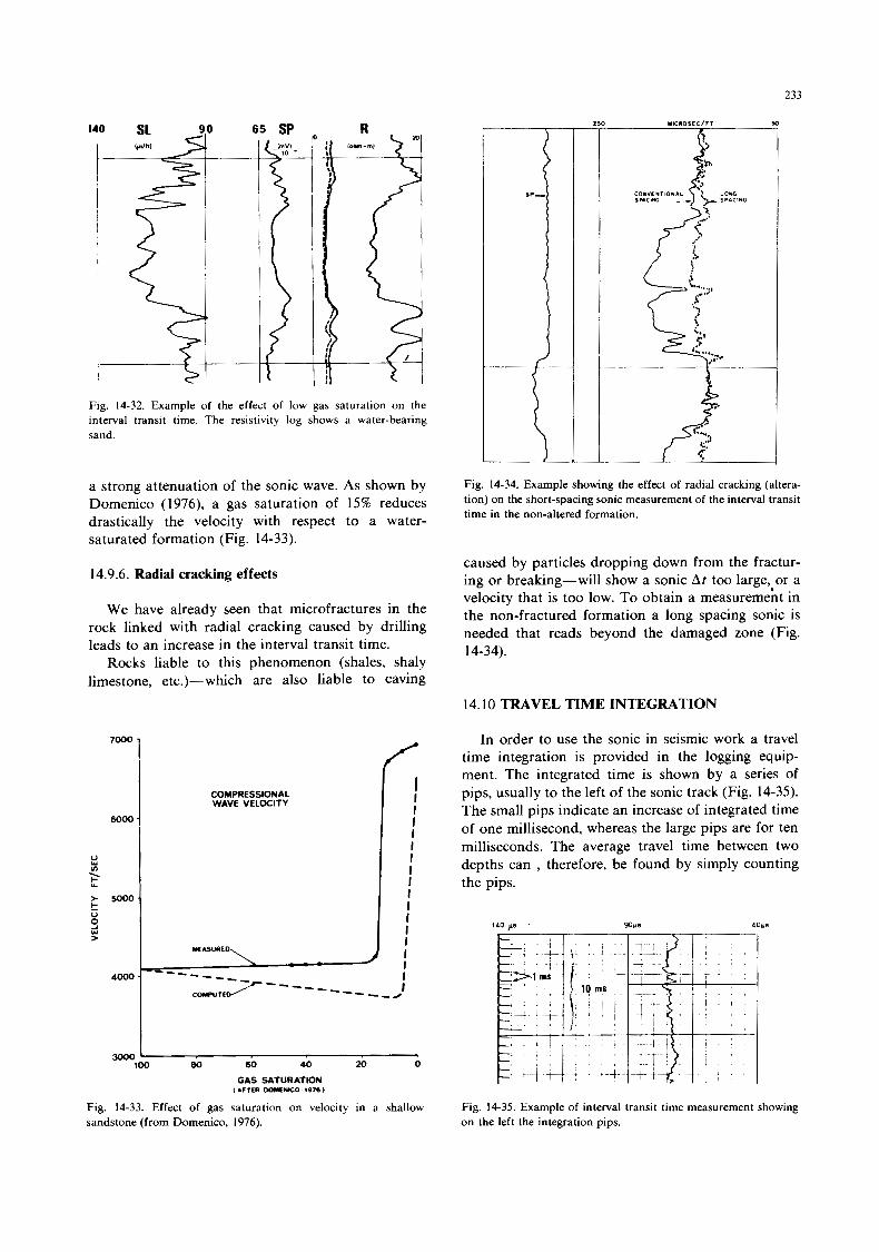
233
6000.
Fig. 14-32. Example of the effect of low gas saturation on the interval transit time. The resistivity log shows a water-bearing sand.
a strong attenuation of the sonic wave. As shown by Domenico (1976), a gas saturation of 15% reduces drastically the velocity with respect to a water- saturated formation (Fig. 14-33).
14.9.6. Radial cracking effects
We have already seen that microfractures in the rock linked with radial cracking caused by drilling leads to an increase in the interval transit time.
Rocks liable to this phenomenon (shales, shaly limestone, etc.)- which are also liable to caving
COMPRESSIONAL WAVE VELOCITY fi I I
>
V c s Y >
80 60 40 20 0 100
GAS SATURATION I AFTER WUENKO 1976 1
Fig. 14-33. Effect of gas saturation on velocity in a shallow sandstone (from Domenico, 1976).
Fig. 14-34. Example showing the effect of radial cracking (altera- tion) on the short-spacing sonic measurement of the interval transit time in the non-altered formation.
caused by particles dropping down from the fractur- ing or breaking-will show a sonic At too large,,or a velocity that is too low. To obtain a measurement in the non-fractured formation a long spacing sonic is needed that reads beyond the damaged zone (Fig. 14-34).
14.10 TRAVEL TIME INTEGRATION
In order to use the sonic in seismic work a travel time integration is provided in the logging equip- ment. The integrated time is shown by a series of pips, usually to the left of the sonic track (Fig. 14-35). The small pips indicate an increase of integrated time of one millisecond, whereas the large pips are for ten milliseconds. The average travel time between two depths can , therefore, be found by simply counting the pips.
Fig. 14-35. Example of interval transit time measurement showing on the left the integration pips.
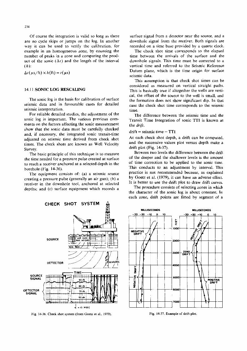
234
Of course the integration is valid so long as there are no cycle skips or jumps on the log. In another way it can be used to verify the calibration, for example in an homogeneous zone, by counting the number of peaks in a zone and comparing the prod- uct of the sonic ( A t ) and the length of the interval (h): At(ps/ft) x h(ft) = t ( p s )
14.1 1 SONIC LOG RESCALING
The sonic log is the basis for calibration of surface seismic data and in favourable cases for detailed seismic interpretation.
For reliable detailed studies, the adjustment of the sonic log is important. The various previous com- ments on the factors affecting the sonic measurement show that the sonic data must be carefully checked and, if necessary, the integrated sonic transit-time adjusted on seismic time derived from check shot times. The check shots are known as Well Velocity Survey.
The basic principle of this technique is to measure the time needed for a pressure pulse created at surface to reach a receiver anchored at a selected depth in the borehole (Fig. 14-36).
The equipment consists of: (a) a seismic source creating a pressure pulse (generally an air gun); (b) a receiver in the downhole tool, anchored at selected depths; and (c) surface equipment which records a
CHECK SHOT SYSTEM
SOURCE
SOURCE SIGNAL
4 b10 MSEC
Fig. 14-36. Check shot system (from Goetz et al., 1979)
surface signal from a detector near the source, and a downhole signal from the receiver. Both signals are recorded on a time base provided by a quartz clock.
The check shot time corresponds to the elapsed time between the arrivals of the surface and the downhole signals. This time must be corrected to a vertical time and referred to the Seismic Reference Datum plane, which is the time origin for surface seismic data.
This assumption is that check shot times can be considered as measured on vertical straight paths. This is basically true if altogether the wells are verti- cal, the offset of the source to the well is small, and the formation does not show significant dip. In that case the check shot time corresponds to the seismic time.
The difference between the seismic time and the Transit Time Integration of sonic TTI is known as the drift.
drift = seismic time - TTI At each check shot depth, a drift can be computed, and the successive values plot versus depth make a drift plot (Fig. 14-37).
Between two levels the difference between the drift of the deeper and the shallower levels is the amount of time correction to be applied to the sonic time. This conducts to an adjustment by interval. This practice is not recommended because, as explained by Goetz et al. (1979), it can have an adverse effect. It is better to use the drift plot to draw drift curves.
The procedure consists of selecting zones in which the character of the sonic log is about constant. In each zone, drift points are fitted by segment of a
MILLISECONDS MILLISECONDS
Fig. 14-37. Example of drift plot.
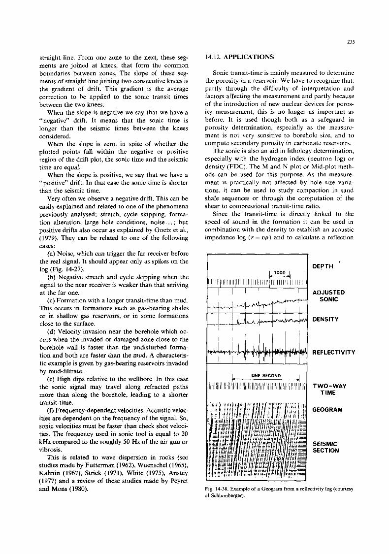
235
14.12. APPLICATIONS
Sonic transit-time is mainly measured to determine the porosity in a reservoir. We have to recognize that, partly through the difficulty of interpretation and factors affecting the measurement and partly because of the introduction of new nuclear devices for poros- ity measurement, this is no longer as important as before. It is used though both as a safeguard in porosity determination, especially as the measure- ment is not very sensitive to borehole size, and to compute secondary porosity in carbonate reservoirs.
The sonic is also an aid in lithology determination, especially with the hydrogen index (neutron log) or density (FDC). The M and N plot or Mid-plot meth- ods can be used for this purpose. As the measure- ment is practically not affected by hole size varia- tions, it can be used to study compaction in sand shale sequences or through the computation of the shear to compressional transit-time ratio.
Since the transit-time is directly linked to the speed of sound in the formation it can be used in combination with the density to establish an acoustic impedance log ( r = u p ) and to calculate a reflection
straight line. From one zone to the next, these seg- ments are joined at knees, that form the common boundaries between zones. The slope of these seg- ments of straight line joining two consecutive knees is the gradient of drift. This gradient is the average correction to be applied to the sonic transit times between the two knees.
When the slope is negative we say that we have a “negative” drift. It means that the sonic time is longer than the seismic times between the knees considered.
When the slope is zero, in spite of whether the plotted points fall within the negative or positive region of the drift plot, the sonic time and the seismic time are equal.
When the slope is positive, we say that we have a “positive” drift. In that case the sonic time is shorter than the seismic time.
Very often we observe a negative drift. This can be easily explained and related to one of the phenomena previously analysed: stretch, cycle skipping, forma- tion alteration, large hole conditions, noise. . . ; but positive drifts also occur as explained by Goetz et al., (1 979). They can be related to one of the following cases:
(a) Noise, which can trigger the far receiver before the real signal. It should appear only as spikes on the log (Fig. 14-27).
(b) Negative stretch and cycle skipping when the signal to the near receiver is weaker than that arriving at the far one.
(c) Formation with a longer transit-time than mud. This occurs in formations such as gas-bearing shales or in shallow gas reservoirs, or in some formations close to the surface.
(d) Velocity invasion near the borehole which oc- curs when the invaded or damaged zone close to the borehole wall is faster than the undisturbed forma- tion and both are faster than the mud. A characteris- tic example is given by gas-bearing reservoirs invaded by mud-filtrate.
(e) High dips relative to the wellbore. In t h s case the sonic signal may travel along refracted paths more than along the borehole, leading to a shorter transit- time.
( f ) Frequency-dependent velocities. Acoustic velw- ities are dependent on the frequency of the signal. So, sonic velocities must be faster than check shot veloci- ties. The frequency used in sonic tool is equal to 20 kHz compared to the roughly 50 Hz of the air gun or vibrosis.
This is related to wave dispersion in rocks (see studies made by Futterman (1962), Wuenschel(1965), Kalinin (1967), Strick (1971), White (1975), Anstey (1977) and a review of these studies made by Peyret and Mons (1980).
DEPTH
ADJUSTED SONIC
DENSITY
REFLECT lVlT V
TWO- WAY TIME
GEOGRAM
SEfSMlC SECTION
Fig. 14-38. Example of a Geogram from a reflectivity log (courtesy of Schlumberger).
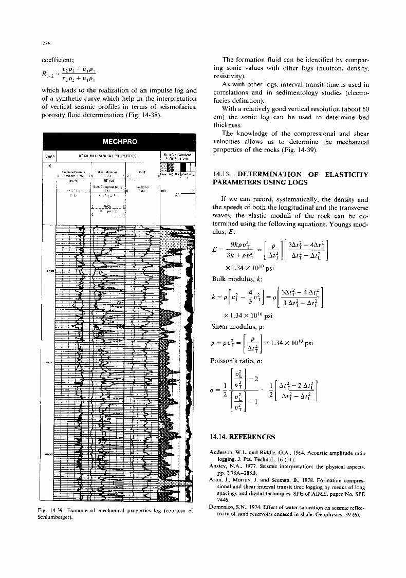
236
coefficient; V2P2 - V I P ,
U2P2 + V I P I RI.2 =
which leads to the realization of an impulse log and of a synthetic curve which help in the interpretation of vertical seismic profiles in terms of seismofacies, porosity fluid determination (Fig. 14-38).
Fig. 14-39. Example of mechanical properties log (courtesy of Schlumberger).
The formation fluid can be identified by compar- ing sonic values with other logs (neutron, density, resistivity).
As with other logs, interval-transit-time is used in correlations and in sedimentology studies (electro- facies definition).
With a relatively good vertical resolution (about 60 cm) the sonic log can be used to determine bed thickness.
The knowledge of the compressional and shear velocities allows us to determine the mechanical properties of the rocks (Fig. 14-39).
14.13. DETERMINATION OF ELASTICITY PARAMETERS USING LOGS
If we can record, systematically, the density and the speeds of both the longitudinal and the transverse waves, the elastic moduli of the rock can be de- -termined using the following equations ulus, E :
E = 9kpv; 3At: - 4Ati
3k + pv; = [ &][ At+-- At:
X 1.34 X 1 O l o psi Bulk modulus, k:
3At: - 4 At: 3 At: - At:
X 1.34 x 10" psi Shear modulus, p:
Poisson's ratio, u:
14.14. REFERENCES
Youngs mod-
*
Anderson, W.L. and Riddle, G.A., 1964. Acoustic amplitude ratio logging. J. Pet. Technol., 16 (1 1).
Anstey, N.A., 1977. Seismic interpretation: the physical aspects. pp. 2.78A-288B.
Aron, J., Murray, J. and Seeman, B., 1978. Formation compres- sional and shear interval transit time logging by means of long spacings and digital techniques. SPE of AIME, paper No. SPE 7446.
Domenico, S.N., 1974. Effect of water saturation on seismic reflec- tivity of sand reservoirs encased in shale. Geophysics, 39 (6).
237
Domenico, S.N., 1976. Effect of brine gas mixture on velocity in an
Dupal, L., Gartner, J. and Vivet, B., 1977. Seismic applications of
Futterman, W.I., 1962. Dispersive body waves: J. Geophys. Res.,
Geerstma, K., 1961. Velocity log interpretation: the effect of rock-bulk compressibility. J. SOC. Pet. Eng., 1.
Goetz, J.F., Dupal, L. and Bowler, J., 1979. An investigation into discrepancies between sonic log and seismic check shot veloci- ties.
Guyod, H. and Shane, L.E., 1969. Geophysical Well Logging, Vol. 1. Guyod, Houston.
Kalinin, A.V., 1967. Estimate of the phase velocity in absorbing media: Izv. Earth Physics (English translation) No. 4, pp. 249-25 1.
Kokesh, F.P., Schwartz, R.J., Wall, W.B. and Morris, R.L., 1960. A new approach to sonic loggng and other acoustic measure- ments. SOC. Petrol. Eng., Paper No. SPE 991. J. Pet. Technol.,
Kowalski, J., 1975. Formation strength parameters from well logs. SPWLA, 16th ann. Log. Symp. Trans., Paper N.
Ladefroux, J., 1961. Mesure en laboratoire de la vitesse du son dans les roches sedimentaires consolidks. Rev. Inst. F r a y . Petrol., 16 (4).
Morlier, P. and Sarda, J.P., 1971. Attenuation des ondes elastiques dans les roches poreuses saturks. Rev. Inst. FranG. Petrol., 26
Morris, R.L., Grine, D.R. and Arkfeld, T.E., 1963. The use of
unconsolidated sand reservoir. Geophysics, 41 (5).
well logs. 5th European Logging Symposium.
67 (13), pp. 5269-5291.
12 (3).
(9).
compressional and shear acoustic amplitudes for location of fractures. SOC. Petrol. Eng., Paper No. SPE 723.
Nations, J.F., 1974. Lithology and porosity from acoustic shear and compressional wave transit time relationships. SPWLA, 15th Annu. Log. Symp. Trans., Paper Q.
Peyret, 0. and Mons, F., 1980. Sonic versus seismic velocities, positive drift study, recording frequency effect.
Pickett, G.R., 1963. Acoustic character logs and their applications in formation evaluation. J. Pet. Technol., 15 (6).
Raymer, L.L., Hunt, E.R. and Gardner, J.S., 1980. An improved sonic transit time to porosity transform. SPWLA, 21st Annu. Log. Symp. Trans., Paper P.
Sarmiento, R., 1961. Geological factors influencing porosity esti- mates from velocity logs. Bul. Am. Assoc. Pet. Geol., 45 (5).
Shumway, G., 1958. Sound velocity vs temperature in water- saturated sediments. Geophysics, 23 (3).
Strick, E., 1971. An explanation of observed time discrepancies between continuous and conventional well velocity survey. Geophysics, 36(2); 285-295.
Summers, G.C. and Broding, R.A., 1952. Continuous velocity logging. Geophysics, 17 (3).
Tixier, M.P., Alger, R.P. and Doh, C.A., 1959. Sonic logging. J. Pet. Technol., 11 (5).
White, J.E., 1975. Computed seismic speeds and attenuation in rocks with partial gas saturation. Geophysics, 40 (2): 224-232.
Wuenschel, P.C., 1965. Dispersive body waves-an experimental study. Geophysics, 3G. 539-551.
Wyllie, M.R.J., Gregory, A.R. and Gardner, L.W., 1956. Elastic wave velocities in heterogeneous and porous media. Geo- physics, 21 (1).

This Page Intentionally Left Blank
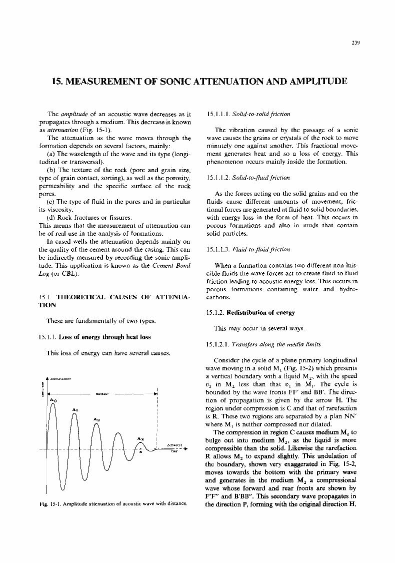
239
15. MEASUREMENT OF SONIC ATTENUATION AND AMPLITUDE
The amplitude of an acoustic wave decreases as it propagates through a medium. This decrease is known as attenuation (Fig. 15-1).
The attenuation as the wave moves through the formation depends on several factors, mainly:
(a) The wavelength of the wave and its type (longi- tudinal or transversal).
(b) The texture of the rock (pore and grain size, type of grain contact, sorting), as well as the porosity, permeability and the specific surface of the rock pores.
(c) The type of fluid in the pores and in particular its viscosity.
(d) Rock fractures or fissures. This means that the measurement of attenuation can be of real use in the analysis of formations.
In cased wells the attenuation depends mainly on the quality of the cement around the casing. This can be indirectly measured by recording the sonic ampli- tude. This application is known as the Cement Bond Log (or CBL).
15.1. THEORETICAL CAUSES OF ATTENUA- TION
15.1.1.1. Solid-to-solid friction
The vibration caused by the passage of a sonic wave causes the grains or crystals of the rock to move minutely one against another. This fractional move- ment generates heat and so a loss of energy. This phenomenon occurs mainly inside the formation.
15.1.1.2. Solid-to-fluid friction
As the forces acting on the solid grains and on the fluids cause different amounts of movement, fric- tional forces are generated at fluid to solid boundaries, with energy loss in the form of heat. This occurs in porous formations and also in muds that contain solid particles.
15.1.1.3. Fluid-to-fluid friction
When a formation contains two different non-his- cible fluids the wave forces act to create fluid to fluid friction leading to acoustic energy loss. This occurs in porous formations containing water and hydro- carbons.
15.1.2. Redistribution of energy These are fundamentally of two types.
This may occur in several ways. 15.1.1. Loss of energy through heat loss
15.1.2.1. Transfers along the media limits This loss of energy can have several causes.
4 DISPLACEMEN7
Fig. 15-1. Amplitude attenuation of acoustic wave with distance.
Consider the cycle of a plane primary longitudinal wave moving in a solid MI (Fig. 15-2) which presents a vertical boundary with a liquid M,, with the speed v2 in M, less than that u1 in M,. The cycle is bounded by the wave fronts FF’ and BB’. The direc- tion of propagation is given by the arrow H. The region under compression is C and that of rarefaction is R. These two regions are separated by a plan NN’ where MI is neither compressed nor dilated.
The compression in region C causes medium M, to bulge out into medium M,, as the liquid is more compressible than the solid. Likewise the rarefaction R allows M, to expand slightly. This undulation of the boundary, shown very exaggerated in Fig. 15-2, moves towards the bottom with the primary wave and generates in the medium M, a compressional wave whose forward and rear fronts are shown by F‘F” and B’BB’’. This secondary wave propagates in the direction P, forming with the original direction H,
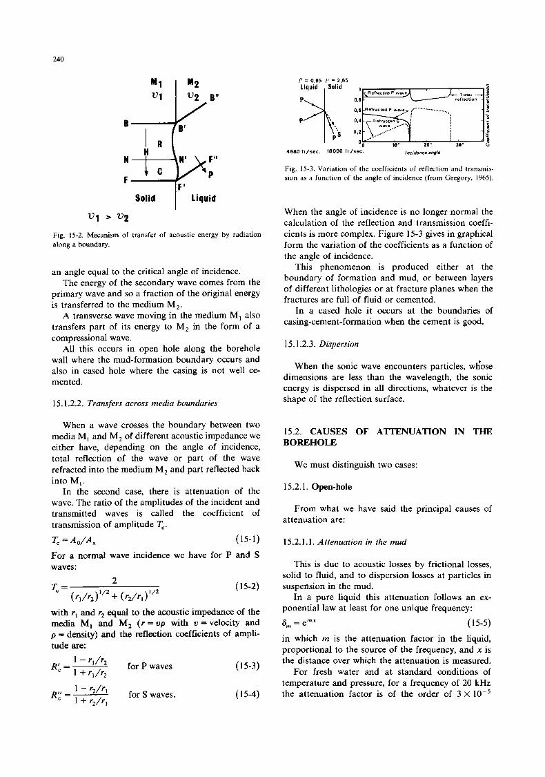
240
Solid I Liquid
*1 ’ v2 Fig. 15-2. Mecanism of transfer of acoustic energy by radiation along a boundary.
an angle equal to the critical angle of incidence. The energy of the secondary wave comes from the
primary wave and so a fraction of the original energy is transferred to the medium M,.
A transverse wave moving in the medium M, also transfers part of its energy to M, in the form of a compressional wave.
All t h s occurs in open hole along the borehole wall where the mud-formation boundary occurs and also in cased hole where the casing is not well ce- mented.
15.1.2.2. Transfers across media boundaries
When a wave crosses the boundary between two media M I and M, of different acoustic impedance we either have, depending on the angle of incidence, total reflection of the wave or part of the wave refracted into the medium M, and part reflected back into M I .
In the second case, there is attenuation of the wave. The ratio of the amplitudes of the incident and transmitted waves is called the coefficient of transmission of amplitude T,. T, = W A X (15-1)
For a normal wave incidence we have for P and S waves:
( 15-2)
with rl and r, equal to the acoustic impedance of the media M, and M, ( r = u p with u=velocity and p = density) and the reflection coefficients of ampli- tude are:
for P waves 1 - r,/r2 R‘, = 1 + r l / r2
- r2’rl for s waves. R’ = 1 + r2/r1
( 15-3)
( 15-4)
Fig. 15-3. Variation of the coefficients of reflection and transmis- sion as a function of the angle of incidence (from Gregory, 1965).
When the angle of incidence is no longer normal the calculation of the reflection and transmission coeffi- cients is more complex. Figure 15-3 gives in graphical form the variation of the coefficients as a function of the angle of incidence.
This phenomenon is produced either at the boundary of formation and mud, or between layers of different lithologies or at fracture planes when the fractures are full of fluid or cemented.
In a cased hole it occurs at the boundaries of casing-cement-formation when the cement is good.
15.1.2.3. Dispersion
When the sonic wave encounters particles, w6ose dimensions are less than the wavelength, the sonic energy is dispersed in all directions, whatever is the shape of the reflection surface.
15.2. CAUSES OF ATTENUATION IN THE BOREHOLE
We must distinguish two cases:
15.2.1. Open-hole
From what we have said the principal causes of attenuation are:
15.2.1.1. Attenuation in the mud
This is due to acoustic losses by frictional losses, solid to fluid, and to dispersion losses at particles in suspension in the mud.
In a pure liquid this attenuation follows an ex- ponential law at least for one unique frequency: 8 m = e m x ( 15-5)
in which m is the attenuation factor in the liquid, proportional to the source of the frequency, and x is the distance over which the attenuation is measured.
For fresh water and at standard conditions of temperature and pressure, for a frequency of 20 kHz the attenuation factor is of the order of 3 x lo-’
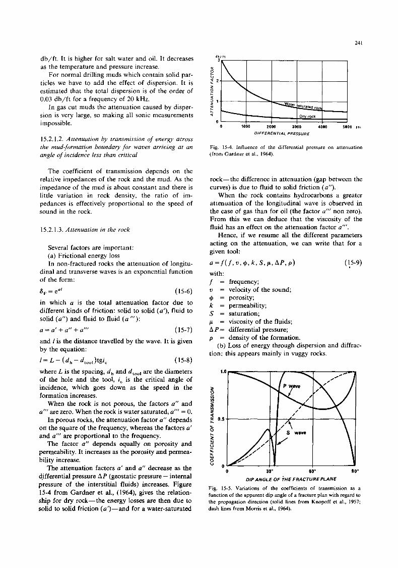
24 1
db/ft. It is higher for salt water and oil. It decreases as the temperature and pressure increase.
For normal drilling muds which contain solid par- ticles we have to add the effect of dispersion. It is estimated that the total dispersion is of the order of 0.03 db/ft for a frequency of 20 kHz.
In gas cut muds the attenuation caused by disper- sion is very large, so making all sonic measurements impossible.
15.2.1.2. Attenuation by transmission of energy across the mud-jormatifn boundary for waves arriving at an angle of incidence less than critical
The coefficient of transmission depends on the relative impedances of the rock and the mud. As the impedance of the mud is about constant and there is little variation in rock density, the ratio of im- pedances is effectively proportional to the speed of sound in the rock.
15.2.1.3. Attenuation in the rock
Several factors are important: (a) Frictional energy loss In non-fractured rocks the attenuation of longitu-
dinal and transverse waves is an exponential function of the form:
8 , = ear ( 15-6)
in which a is the total attenuation factor due to different kinds of friction: solid to solid (a’), fluid to solid (a”) and fluid to fluid (a ’”): a = a’ + a” + a”’ (15-7) and I is the distance travelled by the wave. It is given by the equation:
I = L - (d, - d,,,,)tgi, (1 5-8) where L is the spacing, d , and dtoo, are the diameters of the hole and the tool, i, is the critical angle of incidence, which goes down as the speed in the formation increases.
When the rock is not porous, the factors a” and a”’ are zero. When the rock is water saturated, a”’ = 0.
In porous rocks, the attenuation factor u” depends on\ the square of the frequency, whereas the factors a’ and a”‘ are proportional to the frequency.
The factor a” depends equally on porosity and permeability. It increases as the porosity and permea- bility increase.
The attenuation factors a’ and a” decrease as the differential pressure AP (geostatic pressure - internal pressure of the interstitial fluids) increases. Figure 15-4 from Gardner et al., (1964), gives the relation- ship for dry rock- the energy losses are then due to solid to solid friction (a’)-and for a water-saturated
d b l f t
5000 P S I 0 1000 2000 3000 4000 DIFFERENTIAL PRESSURE
Fig. 15-4. Influence of the differential pressure on attenuation (from Gardner et al., 1964).
with: f =
+ = k = s = c L = AP= P =
(b)
u =
rock-the difference in attenuation (gap between the curves) is due to fluid to solid friction (a”).
When the rock contains hydrocarbons a greater attenuation of the longitudinal wave is observed in the case of gas than for oil (the factor a”’ non zero). From this we can deduce that the viscosity of the fluid has an effect on the attenuation factor a”’.
Hence, if we resume all the different parameters acting on the attenuation, we can write that for a given tool: a = f ( f , * , + , k , S , c L J P , P ) (15-9) .
frequency; velocity of the sound; porosity; permeability ; saturation; viscosity of the fluids; differential pressure; density of the formation. Loss of energy through dispersion and diffrac-
~~
tion: this appears mainly in vuggy rocks.
0 30” 60” 90”
DIP ANGLE OF ?HE FRACTURE PLANE
Fig. 15-5. Variations of the coefficients of transmission as a function of the apparent dip angle of a fracture plan with regard to the propagation direction (solid lines from Knopoff et al., 1957; dash tines from Moms et al., 1964).
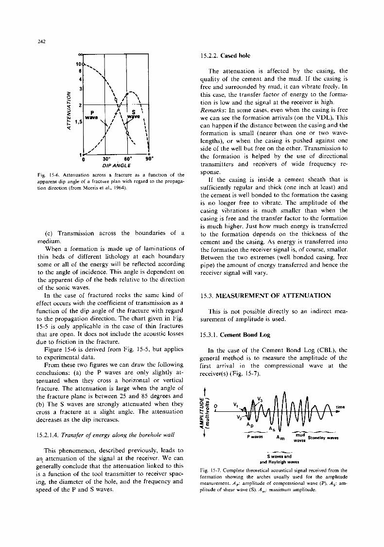
242
DIP ANGLE
Fig. 15-6. Attenuation across a fracture as a function of the apparent dip angle of a fracture plan with regard to the propaga- tion direction (from Morris et al., 1964).
(c) Transmission across the boundaries of a medium.
When a formation is made up of laminations of thin beds of different lithology at each boundary some or all of the energy will be reflected according to the angle of incidence. This angle is dependent on the apparent dip of the beds relative to the direction of the sonic waves.
In the case of fractured rocks the same kind of effect occurs with the coefficient of transmission as a function of the dip angle of the fracture with regard to the propagation direction. The chart given in Fig. 15-5 is only applicable in the case of thin fractures that are open. It does not include the acoustic losses due to friction in the fracture.
Figure 15-6 is derived from Fig. 15-5, but applies to experimental data.
From these two figures we can draw the following conclusions: (a) the P waves are only slightly at- tenuated when they cross a horizontal or vertical fracture. The attenuation is large when the angle of the fracture plane is between 25 and 85 degrees and (b) The S waves are strongly attenuated when they cross a fracture at a slight angle. The attenuation decreases as the dip increases.
15.2.1.4. Transfer of energy along the borehole wall
This phenomenon, described previously, leads to an attenuation of the signal at the receiver. We can generally conclude that the attenuation linked to this is a function of the tool transmitter to receiver spac- ing, the diameter of the hole, and the frequency and speed of the P and S waves.
15.2.2. Cased hole
The attenuation is affected by the casing, the quality of the cement and the mud. If the casing is free and surrounded by mud, it can vibrate freely. In this case, the transfer factor of energy to the forma- tion is low and the signal at the receiver is high. Remarks: In some cases, even when the casing is free we can see the formation arrivals (on the VDL). This can happen if the distance between the casing and the formation is small (nearer than one or two wave- lengths), or when the casing is pushed against one side of the well but free on the other. Transmission to the formation is helped by the use of directional transmitters and receivers of wide frequency re- sponse.
If the casing is inside a cement sheath that is sufficiently regular and thick (one inch at least) and the cement is well bonded to the formation the casing is no longer free to vibrate. The amplitude of the casing vibrations is much smaller than when the casing is free and the transfer factor to the formation is much higher. Just how much energy is transferred to the formation depends on the thickness of the cement and the casing. As energy is transferred into the formation the receiver signal is, of course, smaller. Between the two extremes (well bonded casing, free pipe) the amount of energy transferred and hence the receiver signal will vary.
15.3. MEASUREMENT OF ATTENUATION
This is not possible directly so an indirect mea- surement of amplitude is used.
15.3.1. Cement Bond Log
In the case of the Cement Bond Log (CBL), the general method is to measure the amplitude of the first arrival in the compressional wave at the receiver(s) (Fig. 15-7).
e
_hz_
t Stoneley waves mud
Am waves P waves
S waves and and Rayleigh waves
Fig. 15-7. Complete theoretical acoustical signal received from the formation showing the arches usually used for the amplitude measurement. A,: amplitude of compressional wave (P). A,: am- plitude of shear wave (S). A,: maximum amplitude.
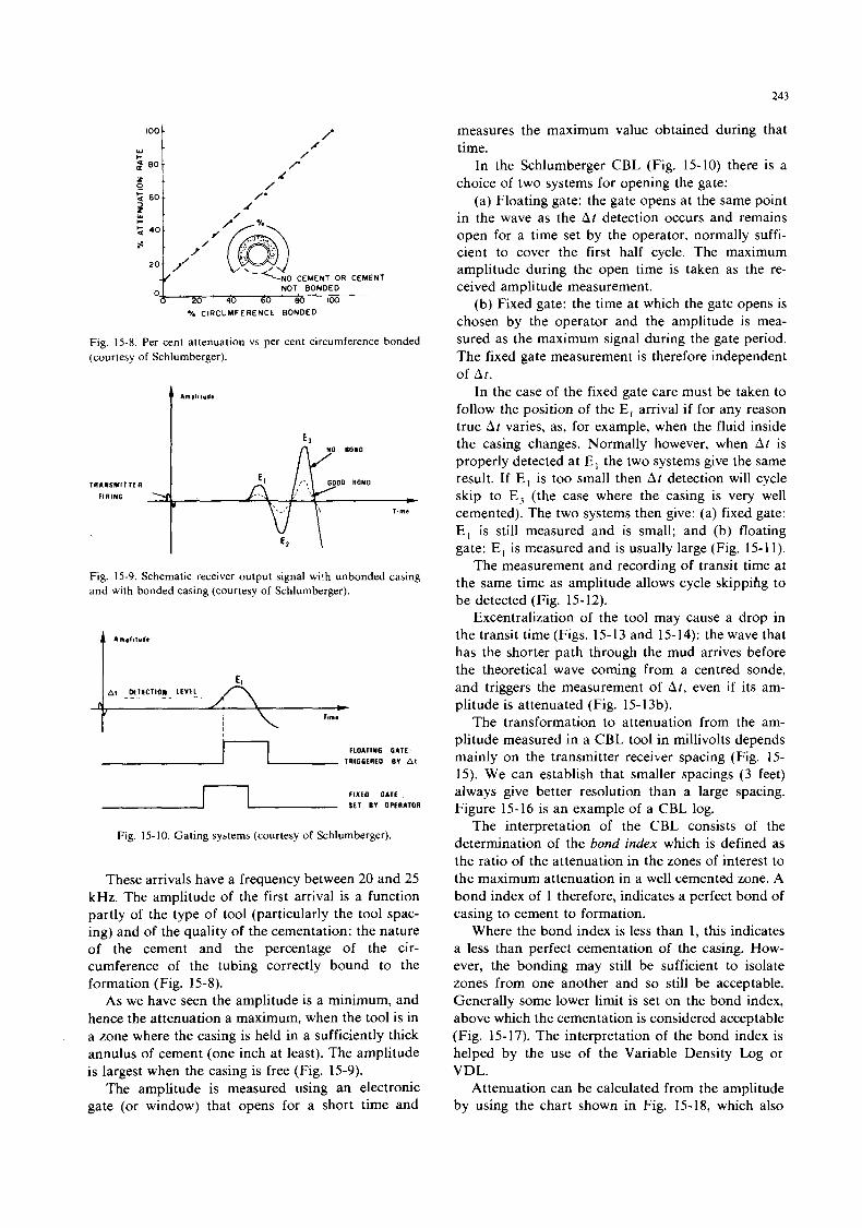
243
5 60. z r W ’
5 4 0 .
8 .
2 0 -
0-
100 1
/ * I
t ,/
/ ‘- <NO CEMENT OR
, NOT BONDED
40 60 80 100
: t 2 80
/ /-
/ /-
I /
CEMENT
*I. CIRCUMFERENCE BONDED
Fig. 15-8. Per cent attenuation vs per cent circumference bonded (courtesy of Schlumberger).
Amplilvdr t I E 3
Fig. 15-9. Schematic receiver output signal wi!h unbonded casing and with bonded casing (courtesy of Schlumberger).
Ampli ludi t
Fig. 15-10. Gating systems (courtesy of Schlumberger).
These arrivals have a frequency between 20 and 25 kHz. The amplitude of the first arrival is a function partly of the type of tool (particularly the tool spac- ing) and of the quality of the cementation: the nature of the cement and the percentage of the cir- cumference of the tubing correctly bound to the formation (Fig. 15-8).
As we have seen the amplitude is a minimum, and hence the attenuation a maximum, when the tool is in a zone where the casing is held in a sufficiently thick annulus of cement (one inch at least). The amplitude is largest when the casing is free (Fig. 15-9).
The amplitude is measured using an electronic gate (or window) that opens for a short time and
measures the maximum value obtained during that time.
In the Schlumberger CBL (Fig. 15-10) there is a choice of two systems for opening the gate:
(a) Floating gate: the gate opens at the same point in the wave as the At detection occurs and remains open for a time set by the operator, normally suffi- cient to cover the first half cycle. The maximum amplitude during the open time is taken as the re- ceived amplitude measurement.
(b) Fixed gate: the time at which the gate opens is chosen by the operator and the amplitude is mea- sured as the maximum signal during the gate period. The fixed gate measurement is therefore independent of A t .
In the case of the fixed gate care must be taken to follow the position of the E, arrival if for any reason true At varies, as, for example, when the fluid inside the casing changes. Normally however, when At is properly detected at E l the two systems give the same result. If E , is too small then A t detection will cycle skip to E, (the case where the casing is very well cemented). The two systems then give: (a) fixed gate: E l is still measured and is small; and (b) floating gate: E l is measured and is usually large (Fig. 15-1 1).
The measurement and recording of transit time at the same time as amplitude allows cycle skippihg to be detected (Fig. 15-12).
Excentralization of the tool may cause a drop in the transit time (Figs. 15-13 and 15-14): the wave that has the shorter path through the mud arrives before the theoretical wave coming from a centred sonde, and triggers the measurement of A t , even if its am- plitude is attenuated (Fig. 15-13b).
The transformation to attenuation from the am- plitude measured in a CBL tool in millivolts depends mainly on the transmitter receiver spacing (Fig. 15- 15). We can establish that smaller spacings (3 feet) always give better resolution than a large spacing. Figure 15-16 is an example of a CBL log.
The interpretation of the CBL consists of the determination of the bond index whch is defined as the ratio of the attenuation in the zones of interest to the maximum attenuation in a well cemented zone. A bond index of 1 therefore, indicates a perfect bond of casing to cement to formation.
Where the bond index is less than 1, this indicates a less than perfect cementation of the casing. How- ever, the bonding may still be sufficient to isolate zones from one another and so still be acceptable. Generally some lower limit is set on the bond index, above which the cementation is considered acceptable (Fig. 15-17). The interpretation of the bond index is helped by the use of the Variable Density Log or VDL.
Attenuation can be calculated from the amplitude by using the chart shown in Fig. 15-18, which also
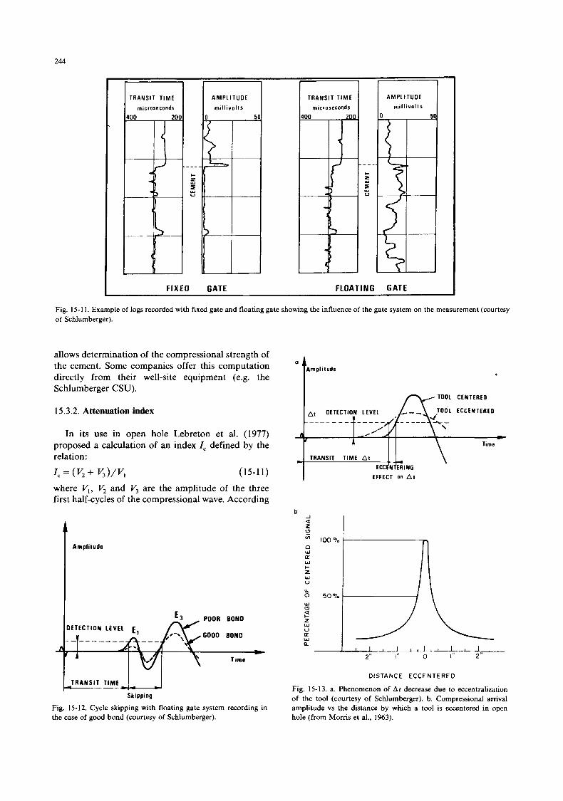
244
FIXED GATE FLOATING GATE
Fig. 15-1 1. Example of logs recorded with fixed gate and floating gate showing the influence of the gate system on the measurement (courtesy of Schlumberger).
allows determination of the compressional strength of the cement. Some companies offer this computation directly from their well-site equipment (e.g. the Schlumberger CSU).
15.3.2. Attenuation index
In its use in open hole Lebreton et al. (1977) proposed a calculation of an index I , defined by the relation:
1, = (V2 + K P , (15-1 1) where V,, V2 and V3 are the amplitude of the three first half-cycles of the compressional wave. According
Amplitude
E3 POOR BONO M
I+ I " l \
J Skipping
Fig. 15-12. Cycle skipping with floating gate system recording in the case of good bond (courtesy of Schlumberger).
Ampl i tude a t TOOL CENTERED
at DETECTION LEVEL TOOL ECCENTEREO
- - Time
TRANSIT T I M E A t
EFFECT on A t
a I I I I I , , I , , 1 1 I 2" I" 0 I" 2"
DI STA N C E ECC E N TE RE D
Fig. 15-13. a. Phenomenon of Ar decrease due to eccentralization of the tool (courtesy of Schlumberger). b. Compressional arrival amplitude vs the distance by which a tool is eccentered in open hole (from Morns et al., 1963).
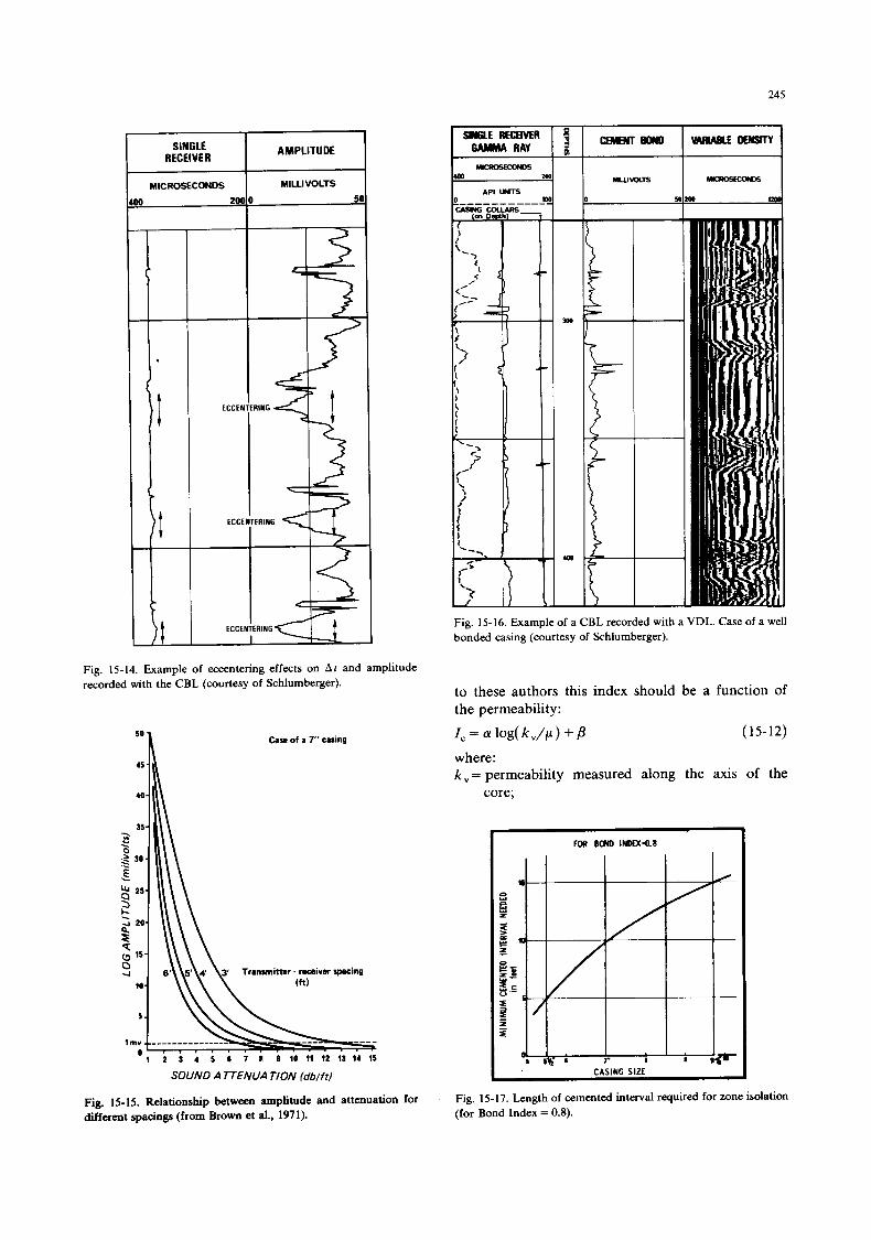
245
SINGLE RECEIVER I
MICROSECONDS MILLIVOLTS
Fig. 15-14. Example of eccentering effects on Ar and amplitude recorded with the CBL (courtesy of Schlumberger).
Care of a 7” casing h
SOUND A TTENUA TION (dblft)
Fig. 15-15. Relationship between amplitude and attenuation for different spacings (from Brown et al., 1971).
SNW RECEIVER GAMMA RAY
MCROSKOlDS Do In
Fig. 15- 16. Example of a CBL recorded with a VDL. Case of a well bonded casing (courtesy of Schlumberger).
to these authors this index should be a function of the permeability:
1, = a log(k,/C1) + P (15-12)
where: k , = permeability measured along the axis of the
core;
FOR Born) INDEX.0.8
Fig. 15-17. Length of cemented interval required for zone isolation (for Bond Index = 0.8).
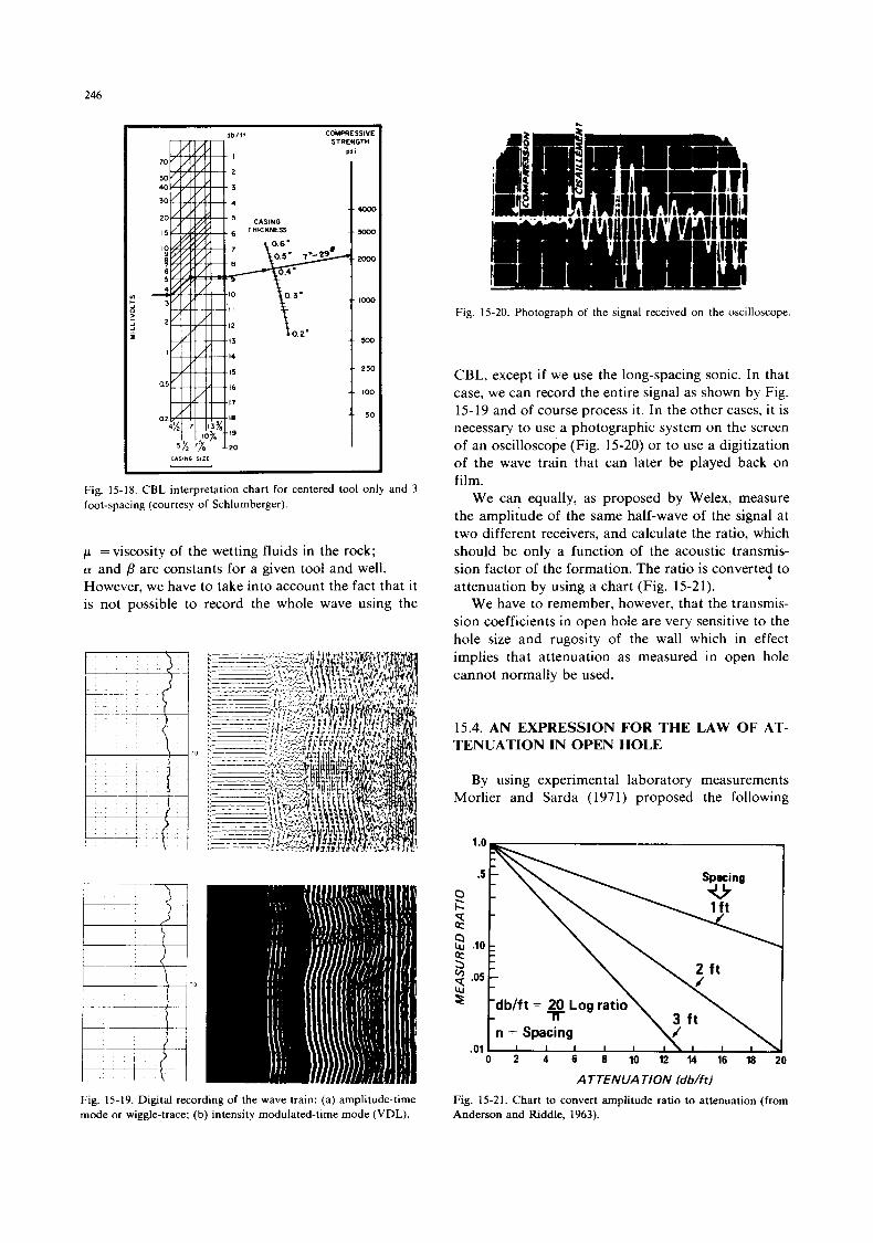
246
d b l f t COMP~IESSIVE STRENGTH
psi
70
4ooo
xxx)
1ooo
lo00
yx)
2 50
I00
50
Fig. 15-18. CBL interpretation chart for centered tool only and 3 foot-spacing (courtesy of Schlumberger).
p, =viscosity of the wetting fluids in the rock; a and p are constants for a given tool and well. However, we have to take into account the fact that i t is not possible to record the whole wave using the
Fig. 15-19. Digital recording of the wave train: (a) amplitude-time mode or wiggle-trace; (b) intensity modulated-time mode (VDL).
Fig. 15-20. Photograph of the signal received on the oscilloscope.
CBL, except if we use the long-spacing sonic. In that case, we can record the entire signal as shown by Fig. 15-19 and of course process it. In the other cases, i t is necessary to use a photographic system on the screen of an oscilloscope (Fig. 15-20) or to use a digitization of the wave train that can later be played back on film.
We can equally, as proposed by Welex, measure the amplitude of the same half-wave of the signal at two different receivers, and calculate the ratio, which should be only a function of the acoustic transmis- sion factor of the formation. The ratio is converte$ to attenuation by using a chart (Fig. 15-21).
We have to remember, however, that the transmis- sion coefficients in open hole are very sensitive to the hole size and rugosity of the wall which in effect implies that attenuation as measured in open hole cannot normally be used.
15.4. AN EXPRESSION FOR THE LAW OF AT- TENUATION IN OPEN HOLE
By using experimental laboratory measurements Morlier and Sarda (1 97 1) proposed the following
A TTENUA TION (db/ft)
Fig. 15-21. Chart to convert amplitude ratio to attenuation (from Anderson and Riddle, 1963).
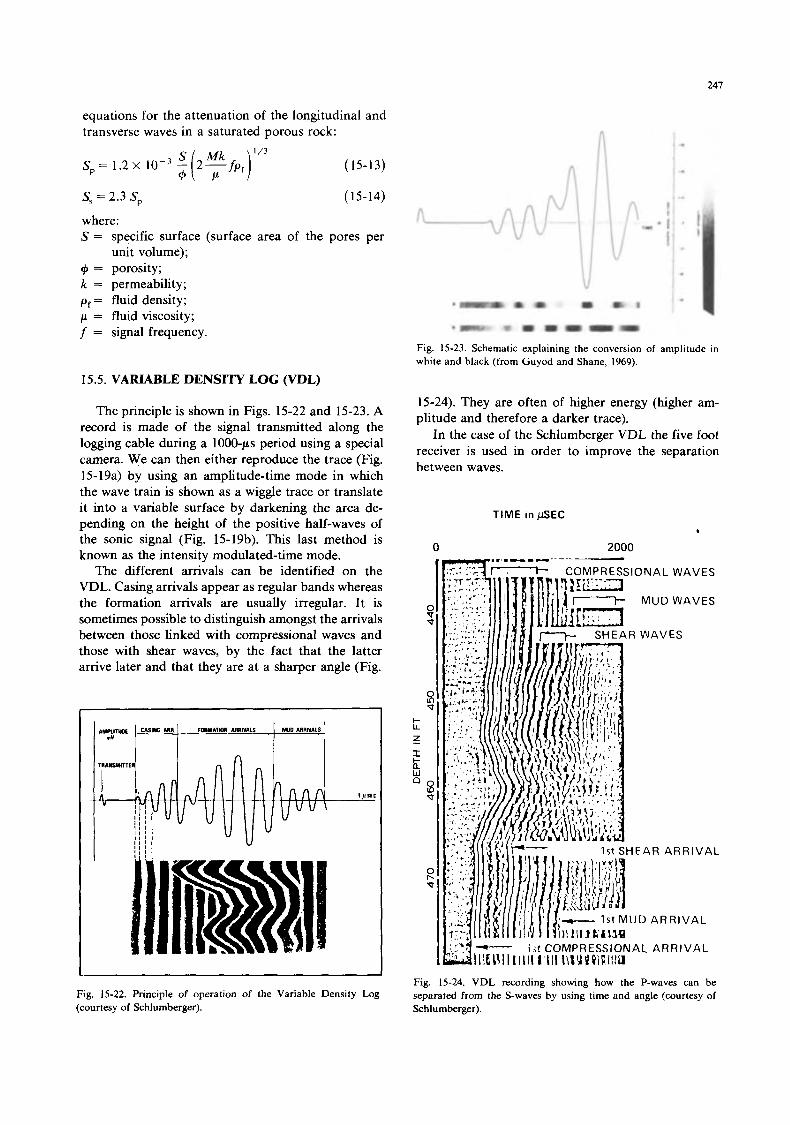
247
equations for the attenuation of the longitudinal and transverse waves in a saturated porous rock:
(15-13)
S, = 2.3 Sp (15-14)
where: S = specific surface (surface area of the pores per
unit volume); + = porosity; k = permeability; pr = fluid density; p = fluid viscosity; f = signal frequency.
Fig. 15-23. Schematic explaining the conversion of amplitude in white and black (from Guyod and Shane, 1969).
15.5. VARIABLE DENSITY LOG (VDL)
The principle is shown in Figs. 15-22 and 15-23. A record is made of the signal transmitted along the logging cable during a 1000-ps period using a special camera. We can then either reproduce the trace (Fig. 15- 19a) by using an amplitude-time mode in which the wave train is shown as a wiggle trace or translate it into a variable surface by darkening the area de- pending on the height of the positive half-waves of the sonic signal (Fig. 15-19b). Thls last method is known as the intensity modulated-time mode.
The different arrivals can be identified on the VDL. Casing arrivals appear as regular bands whereas the formation amvals are usually irregular. It is sometimes possible to distinguish amongst the arrivals between those linked with compressional waves and those with shear waves, by the fact that the latter arrive later and that they are at a sharper angle (Fig.
15-24). They are often of higher energy (higher am- plitude and therefore a darker trace).
In the case of the Schlumberger VDL the five foot receiver is used in order to improve the separation between waves.
Fig. 15-22. Principle of operation of the Variable Density Log (courtesy of Schlumberger).
Fig. 15-24. VDL recording showing how the P-waves can be separated from the S-waves by using time and angle (courtesy of Schlumberger).
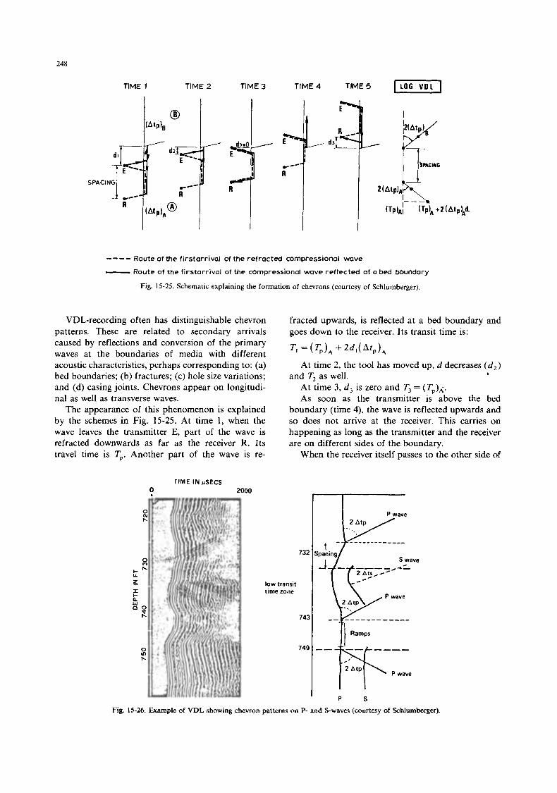
248
TIME 1 TIME 2 TIME 3 TIME 4 TIME5 -1 E'"
, d 5 .
---- Route of the firstarrival of the refracted compressional wave - Route of the firstarrival of the compressional wave reflected at a bed boundary
Fig. 15-25. Schematic explaining the formation of chevrons (courtesy of Schlumberger).
VDL-recording often has distinguishable chevron patterns. These are related to secondary arrivals caused by reflections and conversion of the primary waves at the boundaries of media with different acoustic characteristics, perhaps corresponding to: (a) bed boundaries; (b) fractures; (c) hole size variations; and (d) casing joints. Chevrons appear on longitudi- nal as well as transverse waves.
The appearance of this phenomenon is explained by the schemes in Fig. 15-25. At time 1, when the wave leaves the transmitter E, part of the wave is refracted downwards as far as the receiver R. Its travel time is Tp. Another part of the wave is re-
fracted upwards, is reflected at a bed boundary and goes down to the receiver. Its transit time is:
T I = ( r P > A + 2 d , ( A f p ) A
At time 2, the tool has moved up, d decreases (d2)
At time 3, d, is zero and T3 = (Tp)A,. As soon as the transmitter is above the bed
boundary (time 4), the wave is reflected upwards and so does not arrive at the receiver. This carries on happening as long as the transmitter and the receiver are on different sides of the boundary.
When the receiver itself passes to the other side of
and T, as well. *
rlME IN PSECS
low transit time zone
I P S
Fig. 15-26. Example of VDL showing chevron patterns on P- and S-waves (courtesy of Schlumberger).
0 TIME IN pSECS
249
2000 MWSIlred Computed chevron At
angle b 3 c l f t )
( a t s - 1 3 0 - 1.85) Atp 70
P S
I
chevron slope = A. tg (chewon angle) = A t = 2 A t
VDL scale ratio : A ( 1 )
_ - = lWO 100 wseclinch feethnch 10
A=--
Fig. 15-27. Computation of A I ~ from the slope of the chevron pattern.
the boundary (time 5) it detects once again an arrival reflected from the boundary and at a transit time equal to: have in fact:
This can be done if there are S-chevrons. In this case, At, is given by the gradient (Fig. 15-27). We
An example of chevron patterns is given in Fig.
The main applications of a study of chevron pat-
(A) Fracture detection Depending on the angle that the fracture planes
make with the hole we have to consider three differ- ent cases:
(a) Fractures whose inclination is less than 35". The amplitude of the compression wave is hardly reduced. We can expect only a small amount of reflection. The VDL will have the following char- acteristics: (1) Strong amplitude of the compressional wave (E, or E2); (2) weak or no P-chevron pattern; (3) low amplitude of the shear waves; and (4) well defined S-chevron pattern.
(b) Fractures with an inclination between 35" and 85". The amplitude of the P-wave is reduced. The amplitude of the S-wave goes up and the VDL has the following characteristics: (1) low-amplitude P wave (E, and E2); (2) little or no S-chevron patterns; and (3) some P-chevron patterns.
(c) Fractures with an inclination of over 85". These are very difficult to detect by acoustic methods.
(B) The calculation of At ,
15-26.
terns are:
At, = id/t
We can also calculate it by a method analyzing the whole wave train. The changes in At, are larger than those of At,, which explains why the S-wave arrivals are not parallel to the P-wave arrivals. The difference in time between P- and S-wave arrivals can be ap- proximated by the equation:
T, - Tp = (spacing) (At, - At,) from which we solve for At,:
r,- Tp At, = Atp + ___ spacing
Thus, in the example of Fig, 15-23 between 4277 and 4281 the VDL, whose spacing is five feet, gives:
T, - T, = 200 ps (approx.)
The Atp read by the uncompensated tool is around 45 ps/ft from which we have: At, = 40 + 45 = 85 ps/ft
Remarks: Another method to find At, is to record two VDL's, one with a 3-ft, the other a 5-ft spacing, and to determine the S-wave arrivals on each one. Then, the respective arrival times are measured and the difference divided by 2 ft.
250
15.6. REFERENCES
1 . CBL
Brown, H.D., Grijalva, V.E. and Raymer, L.L., 1971. New de- velopments in sonic wave train display and analysis in cased holes. Log Analyst, 12 (1).
Grosmangin, M. et al., 1960. The Cement Bond Log. Soc. Pet, Eng. AIME, Pasadena Meeting, Paper no. 1512 G.
Grosmanging, M., Kokesh, F.P. and Majani, P., 1961. A sonic method for analyzing the quality of cementation of borehole casings. J. Pet. Technol., 165-171; Trans., AIME, 222.
Muir, D.M. and Latson, B.F., 1962. Oscillographs of acoustic energy and their application to log interpretation. Document P.G.A.C., Houston, 1962.
Pardue, G.H., Moms, R.L., Gollwitzer, L.H., and Moran, J.H., 1963. Cement Bond Log. A study of cement and casing variab- les. Soc. Pet. Eng. AIME, Los Angeles Meeting, Paper No. 453.
Poupon, A., 1964. Interpretation of Cement Bond Logs. Document Schlumberger, Paris.
Putman, L., 1964. A progress Report on Cement Bond Logging. J. Petr. Technol.
Riddle, G.A., 1962. Acoustic Propagation in Bonded and Un- bonded Oil Well Casing. Soc. Pet. Eng. AIME, Los Angeles Meeting, Paper no. 454.
Thurber, C.H. and Latson, B.F., 1960. SATA Log Checks Casing Cement Jobs. Petrol. Eng., Dec. 1960.
Schlumberger, 1976. The essentials of cement evaluation.
2. Attenuation and VDL, VSP
Anderson, W.L. and Riddle, G.A., 1963. Acoustic amplitude ratio logging. Soc. Petr. Eng. AIME, 38th Annu. Fall Meeting, New Orleans, Paper 722.
Anderson, W.L. and Walker, T., 1961. Application of open hole acoustic Amplitude Measurements. Soc. Petr. Eng. AIME, 36th Annu. Fall Meeting, Dallas, Paper 122.
Fons, L.H., 1%3. Use of acoustic signal parameters to locate hydrocarbons and fractured zones. P.G.A.C. Service report, Houston.
Fons, L.H., 1963. Acoustic scope pictures. Soc. Pet. Eng. AIME, 38th Annu. Fall Meeting, New Orleans, Paper 724.
Fons, L.H., 1964. Utilisation des paramktres du signal acoustique pour la localisation directe des hydrocarbures et la determina- tion des zones fracturh. Bull. Assoc. FranG. Techn. PC., 167 (in English: P.G.A.C., no. 64.5).
Gardner, G.H.F., Wyllie, M.R.J. and Droschak, D.M., 1964. Effect of pressure and fluid saturation on the attenuation of the elastic waves in sands. J. Pet. Technol., 16 (2).
Gregory, A.R., 1965. Ultrasonic pulsed-beam transmission and reflection methods for measuring rock properties. Some theo-
retical and experimental results. 6th Annu. Log. Symp. Trans. SPWLA.
Guyod, H. and Shane, L.E., 1969. Geophysical Well Logging, Vol. 1. Guyod, Houston.
Knopoff, L. et al., 1957. 2nd Annual Report, Seismic Scattering Project. Inst. Geophysics, UCLA.
Kokesh, F.P. et al., 1964. A new Approach to sonic Logging and other acoustic measurements. Soc. Pet. Eng. AIME, Paper S.P.E., Houston Meeting, Paper 991.
Lebreton, F., Sarda, J.P., Trocpueme, F. and Morlier, P., 1977. Essais par diagraphie dans des milieux poreux pour evaluer I'influence de leur permeabilite sur des impulsions acoustiques. 5th Europ. Log. Symp. SAID (oct. 1977, Paris).
Morlet and Schwaetzer, 1961. Mesures d'amplitude des ondes soniques dans les sondages. Geophys. Prospect., 9, 4.
Morlet and Schwaetzer, 1962. Le log d'atthuation. 22' reunion EAEG (oct. 1977, Paris).
Morlier, P. and Sarda, J.P., 1971. Attenuation des ondes elastiques dans les roches poreuses saturks.
Moms, R.L., Grine, D.R., Arkfeld, T.E., 1963. The use of com- pressional and shear acoustic amplitudes for the location of fractures. Soc. Pet. Eng. AIME, 38th Annu. Fall Meeting, New Orleans, Paper 723.
Moms, R.L. et al., 1964. Using compressional and shear acoustic amplitudes for the location of fractures. J. Pet. Technol., 16 (6).
Mu&, D.M. and Fons, L.H., 1964. Case histories: Hydrocarbon location from acoustic parameter logs. Trans. S.P.W.L.A. 5th Annu. Log. Symp., 13-15 may 1964.
Muir, D.M. and Fons, L.H., 1964. The new acoustic parameter log: what it is.. . how it operates? World Oil, 'May, 1964.
Pickett, G.R., 1963. Acoustic character logs and their Applications in Formation Evaluation. J. Petrol. Technol., 15, 6.
Schlumberger, 1964. Brevet franpis no 1401258 demande le 2 aw. 1964.
Thurber, C.H., 1961. Acoustic log interpretation. Document P.G.A.C., Houston.
Tixier, M.P., Alger7R. and Doh, C.A., 1959. Sonic Logging. J. Pet. Technol., 11 (5).
Tixier, M.P., Loveless, G.W. and Anderson, R.A., 1973. Estimation of formation strength from the mechanical properties log. SPE of AIME, paper no SPE 4532.
Walker, T., 1962. Fracture Zones Vary Acoustic Signal Ampli- tudes. World Oil, May, 154, 6.
Walker, T., 1962. Progress Report on Aco,ptic Amplitude Logging for Formation Evaluation. Soc. Pet. Eng. AIME, 37th Annu. Fall Meeting, Los Angeles, Paper 451.
Walker, T. and Riddle, G., 1963. Field investigation of full acous- tic wave recording. 4th Annu. Log. Symp. SPWLA.
Wyllie, M.R.J., Gardner, G.H.F. and Gregory, A.R., 1962. Studies of elastic wave attenuation in porous media. Geophysics, 27 (5).
.
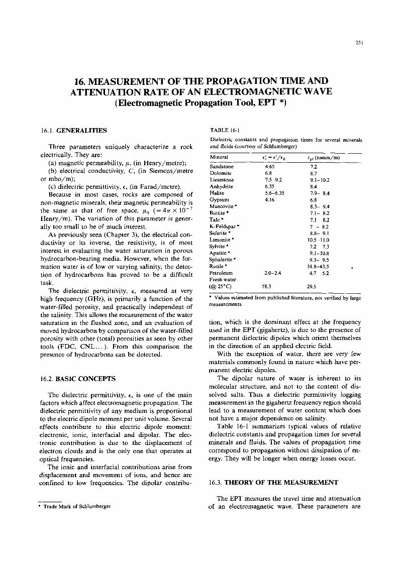
25 1
16. MEASUREMENT OF THE PROPAGATION TIME AND ATTENUATION RATE OF AN ELECTROMAGNETIC WAVE
(Electromagnetic Propagation Tool, EPT *)
16.1. GENERALITIES
Three parameters uniquely characterize a rock
(a) magnetic permeability, p , (in Henry/metre); (b) electrical conductivity, C, (in Siemens/metre
(c) dielectric permittivity, c , (in Farad/metre). Because in most cases, rocks are composed of
non-magnetic minerals, their magnetic permeability is the same as that of free space, po (= 477 X lo-' Henry/m). The variation of ths parameter is gener- ally too small to be of much interest.
As previously seen (Chapter 3), the electrical con- ductivity or its inverse, the resistivity, is of most interest in evaluating the water saturation in porous hydrocarbon-bearing media. However, when the for- mation water is of low or varying salinity, the detec- tion of hydrocarbons has proved to be a difficult task.
The dielectric permittivity, c, measured at very hgh frequency (GHz), is primarily a function of the water-filled porosity, and practically independent of the salinity. This allows the measurement of the water saturation in the flushed zone, and an evaluation of moved hydrocarbon by comparison of the water-filled porosity with other (total) porosities as seen by other tools (FDC, CNL.. . ). From this comparison the presence of hydrocarbons can be detected.
electrically. They are:
or mho/m);
16.2. BASIC CONCEPTS
The dielectric permittivity, c, is one of the main factors which affect electromagnetic propagation. The dielectric permittivity of any medium is proportional to the electric dipole moment per unit volume. Several effects contribute to this electric dipole moment: electronic, ionic, interfacial and dipolar. The elec- tronic contribution is due to the displacement of electron clouds and is the only one that operates at optical frequencies.
The ionic and interfacial contributions arise from displacement and movement of ions, and hence are confined to low frequencies. The dipolar contribu-
TABLE 16-1
Dielectric constants and propagation times for several minerals and fluids (courtesy of Schlumberger)
Mineral r; = €'/C0 r,, (nanos/m)
Sandstone Dolomite Limestone Anhydrite Halite Gypsum Muscovite * Biotite * Talc * K-Feldspar * Siderite * Limonite * Sylvite * Apatite * Sphalerite * Rutile * Petroleum Fresh water (@ 25OC)
4.65 6.8 7.5-9.2 6.35
4.16 5.6-6.35
2.0-2.4
78.3
1.2 8.7 9.1- 10.2 8.4
6.8
7.1- 8.2 7.1- 8.2 7 - 8.2
7.9- 8.4
8.3- 9.4
8.8- 9.1 10.5-1 1.0 1.2- 7.3 9.1- 10.8 9.3- 9.5
4.1- 5.2 31.8-43.5 . 29.5
* Values estimated from published literature, not verified by large measurements.
tion, which is the dominant effect at the frequency used in the EPT (gigahertz), is due to the presence of permanent dielectric dipoles which orient themselves in the direction of an applied electric field.
With the exception of water, there are very few materials commonly found in nature which have per- manent electric dipoles.
The dipolar nature of water is inherent to its molecular structure, and not to the content of dis- solved salts. Thus a dielectric permittivity logging measurement in the gigahertz frequency region should lead to a measurement of water content which does not have a major dependence on salinity.
Table 16-1 summarizes typical values of relative dielectric constants and propagation times for several minerals and fluids. The values of propagation time correspond to propagation without dissipation of en- ergy. They will be longer when energy losses occur.
16.3. THEORY OF THE MEASUREMENT
* Trade Mark of Schlumberger The EFT measures the travel time and attenuation
of an electromagnetic wave. These parameters are
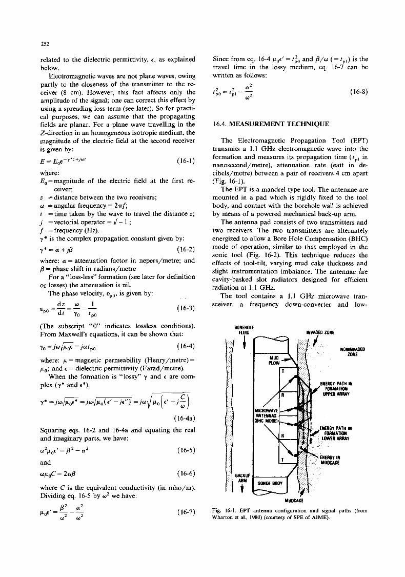
252
related to the dielectric permittivity, e, as explained below.
Electromagnetic waves are not plane waves, owing partly to the closeness of the transmitter to the re- ceiver (8 cm). However, this fact affects only the amplitude of the signal; one can correct this effect by using a spreading loss term (see later). So for practi- cal purposes, we can assume that the propagating fields are planar. For a plane wave travelling in the Z-direction in an homogeneous isotropic medium, the magnitude of the electric field at the second receiver is given by:
E = E0e-Y*‘+JWf (16-1)
where: Eo=magnitude of the electric field at the first re-
z =distance between the two receivers; w = angular frequency = 2 ?r f; t =time taken by the wave to travel the distance z; j =vectorial operator = J-1; f =frequency (Hz). y* is the complex propagation constant given by:
ceiver;
y * = a + j p (16-2) where: a = attenuation factor in nepers/metre; and p = phase shift in radians/metre
For a “loss-less” formation (see later for definition or losses) the attenuation is nil.
The phase velocity, up0, is given by:
(16-3)
(The subscript “0” indicates lossless conditions). From Maxwell’s equations, it can be shown that:
yo = j w t p o ( 16-4)
where: p = magnetic permeability (Henry/metre) =
po; and c = dielectric permittivity (Farad/metre). When the formation is “lossy” y and e are com-
plex (y* and e*).
y* = j w p = j w / m = j w / p o ( ec -j:)
( 16-4a)
Squaring eqs. 16-2 and 16-4a and equating the real and imaginary parts, we have:
w2p0cf = p2 - a2 ( 16-5)
and wpoc = 2ap (16-6)
where C is the equivalent conductivity (in mho/m). Dividing eq. 16-5 by w2 we have:
p2 a2 pocf = - - - w2 w2
(16-7)
Since from eq. 16-4 pot' = tio and p / w (= r p l ) is the travel time in the lossy medium, eq. 16-7 can be written as follows:
aL tp20 = tp21 - -
w2 ( 16-8)
16.4. MEASUREMENT TECHNIQUE
The Electromagnetic Propagation Tool (EFT) transmits a 1.1 GHz electromagnetic wave into the formation and measures its propagation time ( r p l in nanosecond/metre), attenuation rate (eatt in de- cibels/metre) between a pair of receivers 4 cm apart (Fig. 16-1).
The EFT is a mandrel type tool. The antennae are mounted in a pad whch is rigidly fixed to the tool body, and contact with the borehole wall is achieved by means of a powered mechanical back-up arm.
The antenna pad consists of two transmitters and two receivers. The two transmitters are alternately energized to allow a Bore Hole Compensation (BHC) mode of operation, similar to that employed in the sonic tool (Fig. 16-2). This technique reduces the effects of tool-tilt, varying mud cake thickness and slight instrumentation imbalance. The antennae ire cavity-basked slot radiators designed for efficient radiation at 1.1 GHz.
The tool contains a 1.1 GHz microwave tran- sceiver, a frequency down-converter and low-
BOREHOLE FLUID INVADED ZONE
BACKUP ARM
t
NONINVAOEO
ENERGY PATH IN
ENERGY PATH IN
Fig. 16-1. EFT antenna configuration and signal paths (from Wharton et al., 1980) (courtesy of SPE of AIME).
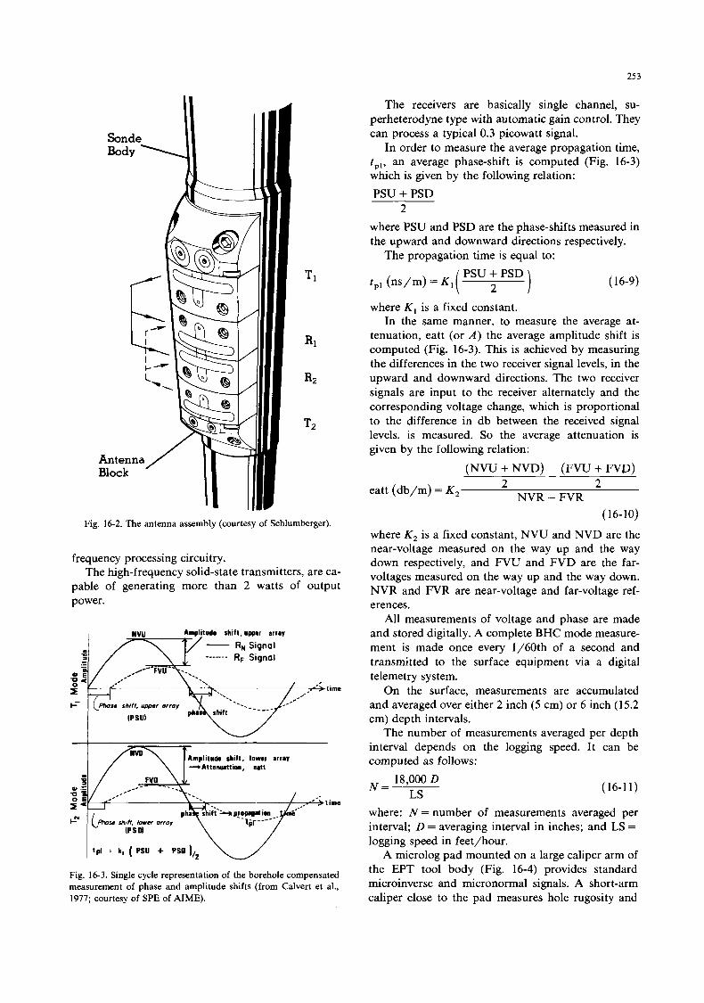
253
Fig. 16-2. The antenna assembly (courtesy of Schlumberger).
frequency processing circuitry. The high-frequency solid-state transmitters, are ca-
pable of generating more than 2 watts of output power.
.time
W
shift, lower array I / --Attatmattion, eitt
/ (PSM
Fig. 16-3. Single cycle representation of the borehole compensated measurement of phase and amplitude shifts (from Calvert et al., 1977; courtesy of SPE of AIME).
The receivers are basically single channel, su- perheterodyne type with automatic gain control. They can process a typical 0.3 picowatt signal.
In order to measure the average propagation time, t , , , an average phase-shift is computed (Fig. 16-3) which is given by the following relation: PSU + PSD
2 where PSU and PSD are the phase-shifts measured in the upward and downward directions respectively.
The propagation time is equal to:
( 16-9)
where K , is a fixed constant. In the same manner, to measure the average at-
tenuation, eatt (or A ) the average amplitude shift is computed (Fig. 16-3). This is achieved by measuring the differences in the two receiver signal levels, in the upward and downward directions. The two receiver signals are input to the receiver alternately and the corresponding voltage change, which is proportional to the difference in db between the received signal levels, is measured. So the average attenuation is given by the following relation:
(NVU + NVD) - (FVU + FVP) 2 2
NVR - FVR eatt (db/m) = K ,
( 16- 10)
where K , is a fixed constant, NVU and NVD are the near-voltage measured on the way up and the way down respectively, and FVU and FVD are the far- voltages measured on the way up and the way down. NVR and FVR are near-voltage and far-voltage ref- erences.
All measurements of voltage and phase are made and stored digitally. A complete BHC mode measure- ment is made once every 1/60th of a second and transmitted to the surface equipment via a digital telemetry system.
On the surface, measurements are accumulated and averaged over either 2 inch (5 cm) or 6 inch (1 5.2 cm) depth intervals.
The number of measurements averaged per depth interval depends on the logging speed. It can be computed as follows:
18,000 D LS
N = (16-1 1)
where: N = number of measurements averaged per interval; D = averaging interval in inches; and LS =
logging speed in feet/hour. A microlog pad mounted on a large caliper arm of
the EPT tool body (Fig. 16-4) provides standard microinverse and micronormal signals. A short-arm caliper close to the pad measures hole rugosity and
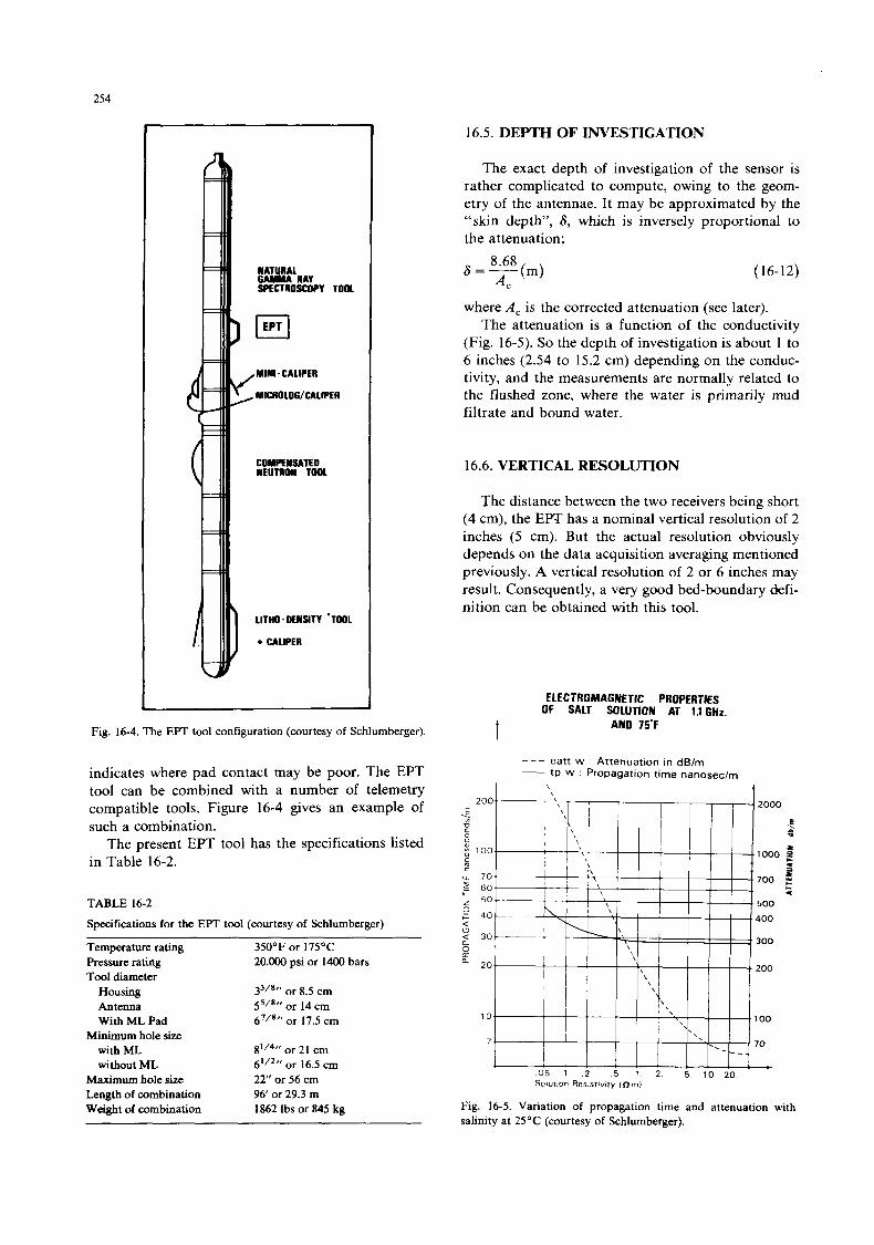
254
NATURAL 6- RAY sPEcTRoxoPv TOOL
)El
COMPENSATED NEUTROll TOOL
LITHO-DENSITY ‘TOOL
+ CALIPER I Fig. 16-4. The EFT tool configuration (courtesy of Schlumberger).
indicates where pad contact may be poor. The EPT tool can be combined with a number of telemetry compatible tools. Figure 16-4 gives an example of such a combination.
The present EFT tool has the specifications listed in Table 16-2.
TABLE 16-2
Specifications for the EFT tool (courtesy of Schlumberger)
Temperature rating 350°F or 175OC Pressure rating Tool diameter Housing 33/8” or 8.5 cm
or 14cm Antenna With ML Pad
Minimum hole size with ML without ML
20.000 psi or 1400 bars
55/8,r
6’/’” or 17.5 cm
8’/4” or 21 cm 6’/”’ or 16.5 cm 22” or 56 cm 96‘ or 29.3 m 1862 Ibs or 845 kg
Maximum hole size Length of combination Weight of combination
16.5. DEPTH OF INVESTIGATION
The exact depth of investigation of the sensor is rather complicated to compute, owing to the geom- etry of the antennae. It may be approximated by the “skin depth”, S, which is inversely proportional to the attenuation;
(16-12)
where A , is the corrected attenuation (see later). The attenuation is a function of the conductivity
(Fig. 16-5). So the depth of investigation is about 1 to 6 inches (2.54 to 15.2 cm) depending on the conduc- tivity, and the measurements are normally related to the flushed zone, where the water is primarily mud filtrate and ‘bound water.
16.6. VERTICAL RESOLUTION
The distance between the two receivers being short (4 cm), the EPT has a nominal vertical resolution of 2 inches (5 cm). But the actual resolution obviously depends on the data acquisition averaging mentioned previously. A vertical resolution of 2 or 6 inches may result. Consequently, a very good bed-boundary defi- nition can be obtained with this tool.
ELECTROMAGNETIC PROPERTIES OF SALT SOLUTION AT 1.lGHz.
AND 75’F
--- eatt w : Attenuation in dElm - tp w : Propagation time nanosec/rn
Fig. 16-5. Variation of propagation time and attenuation with salinity at 25OC (courtesy of Schlumberger).
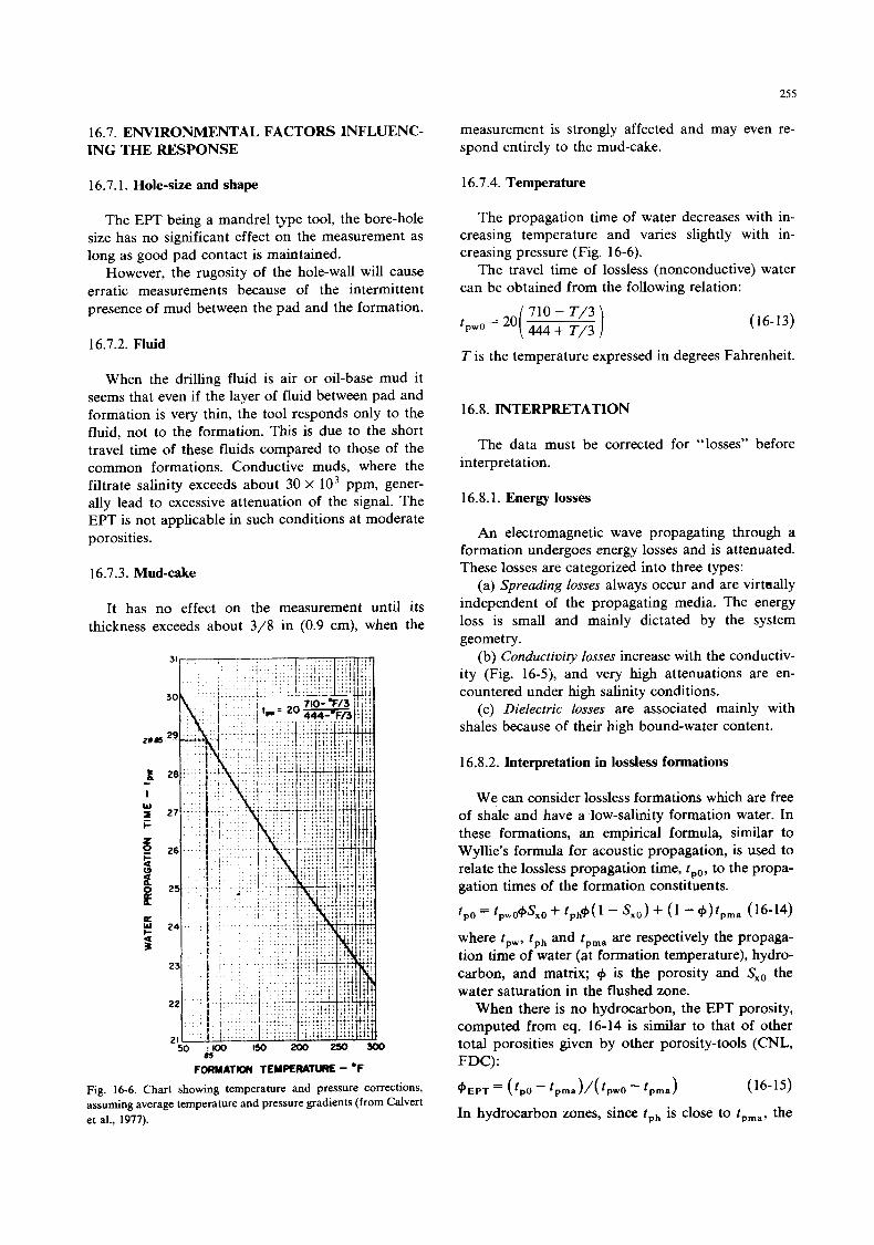
255
16.7. ENVIRONMENTAL FACTORS INFLUENC- ING THE RESPONSE
16.7.1. Hole-size and shape
The EPT being a mandrel type tool, the bore-hole size has no significant effect on the measurement as long as good pad contact is maintained.
However, the rugosity of the hole-wall will cause erratic measurements because of the intermittent presence of mud between the pad and the formation.
16.7.2. Fluid
When the drilling fluid is air or oil-base mud it seems that even if the layer of fluid between pad and formation is very thin, the tool responds only to the fluid, not to the formation. This is due to the short travel time of these fluids compared to those of the common formations. Conductive muds, where the filtrate salinity exceeds about 30 X lo3 ppm, gener- ally lead to excessive attenuation of the signal. The EFT is not applicable in such conditions at moderate porosities.
16.7.3. Mud-cake
It has no effect on the measurement until its thickness exceeds about 3/8 in (0.9 cm), when the
FORMATIW TEMPERATURE - *F
Fig. 16-6. Chart showing temperature and pressure corrections, assuming average temperature and pressure gradients (from Calvert et al., 1977).
measurement is strongly affected and may even re- spond entirely to the mud-cake.
16.7.4. Temperature
The propagation time of water decreases with in- creasing temperature and varies slightly with in- creasing pressure (Fig. 16-6).
The travel time of lossless (nonconductive) water can be obtained from the following relation:
(16-13)
T is the temperature expressed in degrees Fahrenheit.
16.8. INTERPRETATION
The data must be corrected for “losses” before interpretation.
16.8.1. Energy losses
An electromagnetic wave propagating through a formation undergoes energy losses and is attenuated. These losses are categorized into three types:
(a) Spreading losses always occur and are virtually independent of the propagating media. The energy loss is small and mainly dictated by the system geometry.
(b) C o n d u c t i v i t y losses increase with the conductiv- ity (Fig. 16-5), and very high attenuations are en- countered under high salinity conditions.
(c) Dielectric losses are associated mainly with shales because of their high bound-water content.
16.8.2. Interpretation in lossless formations
We can consider lossless formations which are free of shale and have a low-salinity formation water. In these formations, an empirical formula, similar to Wyllie’s formula for acoustic propagation, is used to relate the lossless propagation time, tpO, to the propa- gation times of the formation constituents.
tpO = tpwO+SxO+ lph+( l - ’%O) + ( l - +)tpma (16-14) where tPW, tph and tpma are respectively the propaga- tion time of water (at formation temperature), hydro- carbon, and matrix; + is the porosity and Sxo the water saturation in the flushed zone.
When there is no hydrocarbon, the EFT porosity, computed from eq. 16-14 is similar to that of other total porosities given by other porosity-tools (CNL, FDC):
+EpT = ( tpo - tpma)/(tpwO - tpma) (16-15)
In hydrocarbon zones, since tDh is close to fpma, the
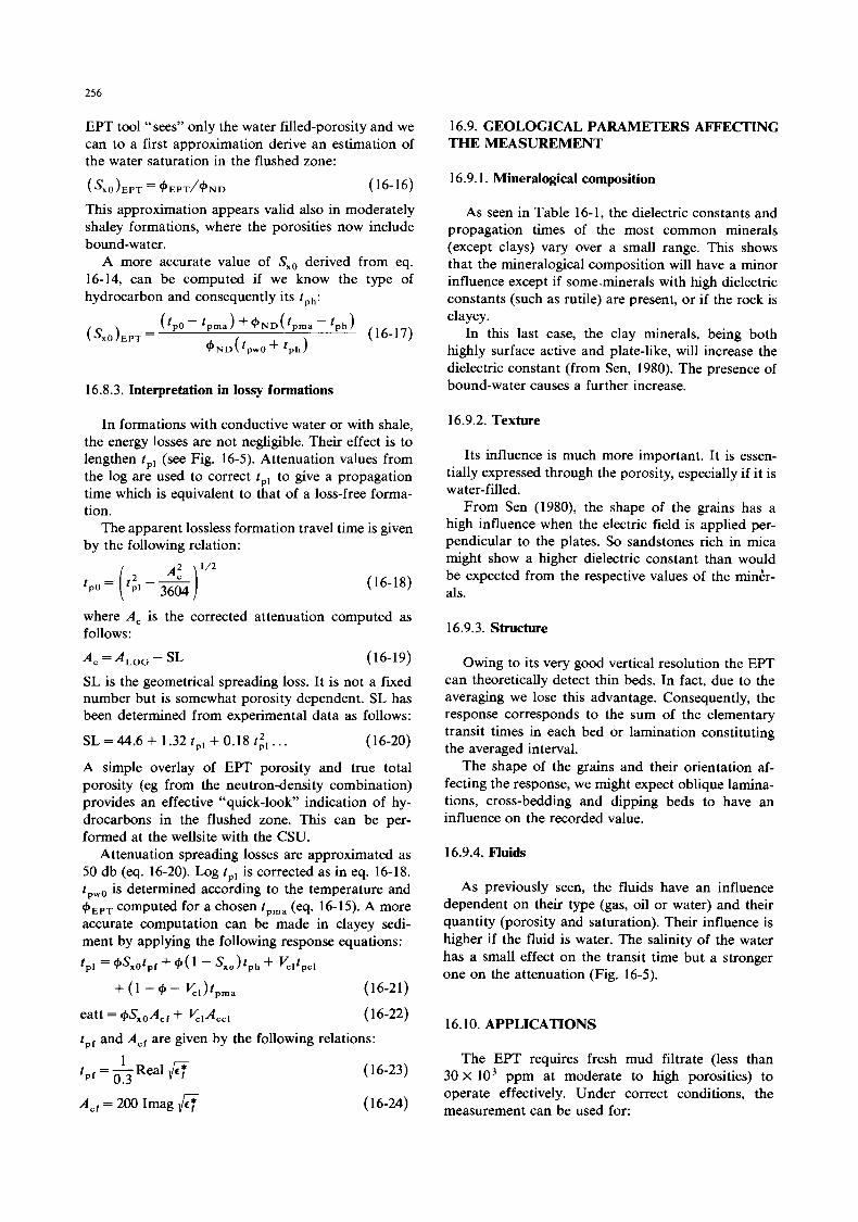
256
EPT tool “sees” only the water filled-porosity and we can to a first approximation derive an estimation of the water saturation in the flushed zone: (sxo),p, = +EPT/+ND (16-16)
This approximation appears valid also in moderately shaley formations, where the porosities now include bound-water.
A more accurate value of Sxo derived from eq. 16-14, can be computed if we know the type of hydrocarbon and consequently its rph:
(Sxo)EPT = (‘PO - ‘prna) ++ND( tp rna - ‘ph) (16-17)
G N D (‘pwO + ‘ph)
16.8.3. Interpretation in lossy formations
In formations with conductive water or with shale, the energy losses are not negligible. Their effect is to lengthen t,, (see Fig. 16-5). Attenuation values from the log are used to correct tp, to give a propagation time which is equivalent to that of a loss-free forma- tion.
The apparent lossless formation travel time is given by the following relation:
(16-18)
where A , is the corrected attenuation computed as follows: A , = A,,, - SL (16-19)
SL is the geometrical spreading loss. It is not a fixed number but is somewhat porosity dependent. SL has been determined from experimental data as follows:
SL = 44.6 + 1.32 rpl + 0.18 f i l . . . ( 16-20)
A simple overlay of EPT porosity and true total porosity (eg from the neutron-density combination) provides an effective “quick-look” indication of hy- drocarbons in the flushed zone. This can be per- formed at the wellsite with the CSU.
Attenuation spreading losses are approximated as 50 db (eq. 16-20). Log t , , is corrected as in eq. 16-18. tpwO is determined according to the temperature and +EPT computed for a chosen tpma (eq. 16-15). A more accurate computation can be made in clayey sedi- ment by applying the following response equations: t , , = W x o t , , + + ( I - Sxoh, , + K’,,‘,,’,,
(16-2 1)
eatt = ~ S x o A , , + VclAccl ( 16-22)
t , , and A,, are given by the following relations:
Real fi t =- pf 0.3
1 (16-23)
A, , = 200 Imag fi ( 16-24)
16.9. GEOLOGICAL PARAMETERS AFFECTING THE MEASUREMENT
16.9.1. Mineralogical composition
As seen in Table 16-1, the dielectric constants and propagation times of the most common minerals (except clays) vary over a small range. This shows that the mineralogical composition will have a minor influence except if someminerals with high dielectric constants (such as rutile) are present, or if the rock is clayey.
In this last case, the clay minerals, being both highly surface active and plate-like, will increase the dielectric constant (from Sen, 1980). The presence of bound-water causes a further increase.
16.9.2. Texture
Its influence is much more important. It is essen- tially expressed through the porosity, especially if it is water-filled.
From Sen (1980), the shape of the grains has a high influence when the electric field is applied per- pendicular to the plates. So sandstones rich in mica might show a higher dielectric constant than would be expected from the respective values of the minkr- als.
16.9.3. Structure
Owing to its very good vertical resolution the EFT can theoretically detect t h n beds. In fact, due to the averaging we lose this advantage. Consequently, the response corresponds to the sum of the elementary transit times in each bed or lamination constituting the averaged interval.
The shape of the grains and their orientation af- fecting the response, we might expect oblique lamina- tions, cross-bedding and dipping beds to have an influence on the recorded value.
16.9.4. Fluids
As previously seen, the fluids have an influence dependent on their type (gas, oil or water) and their quantity (porosity and saturation). Their influence is higher if the fluid is water. The salinity of the water has a small effect on the transit time but a stronger one on the attenuation (Fig. 16-5).
16.10. APPLICATIONS
The EFT requires fresh mud filtrate (less than 30 X lo3 ppm at moderate to high porosities) to operate effectively. Under correct conditions, the measurement can be used for:
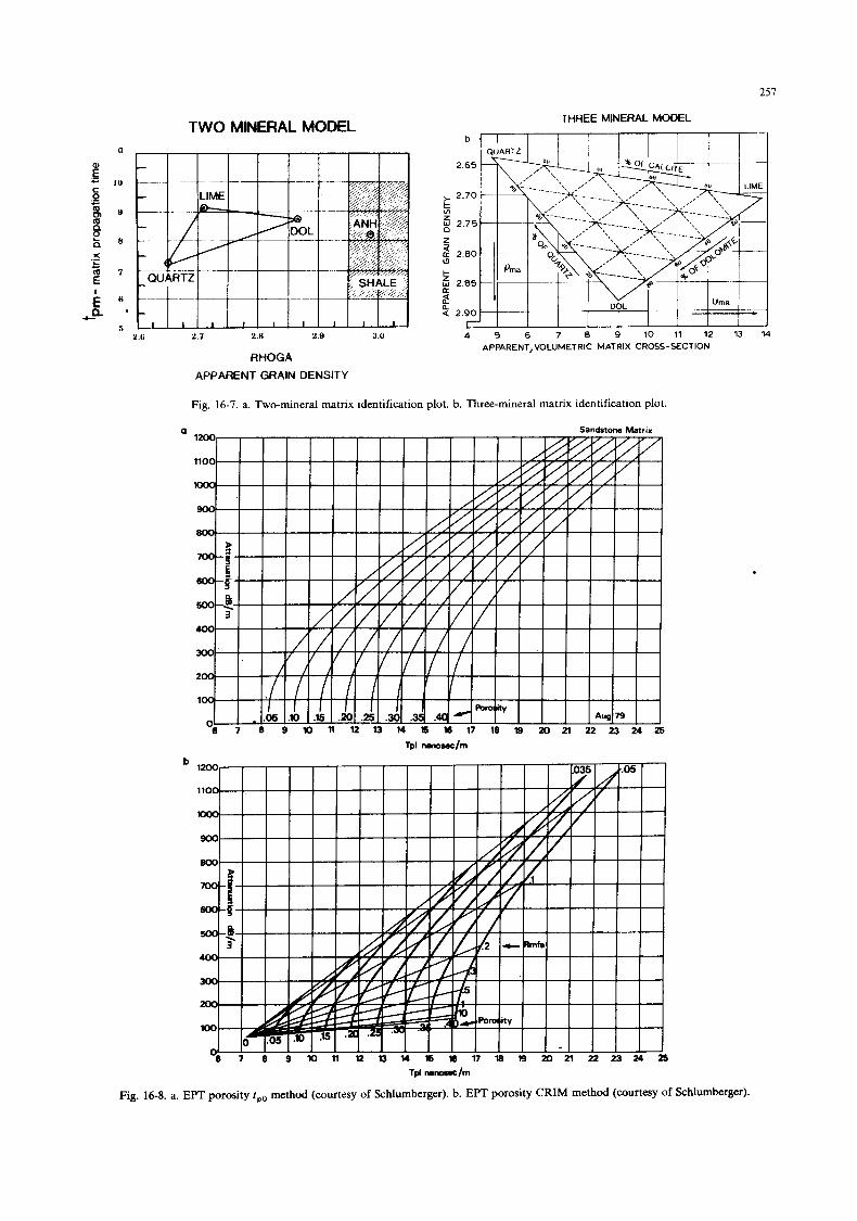
TWO MINERAL MODEL a
I l l
Y
8
7
6
5 2.G 2.7 2.8 2.9 3.0
RHOGA
APPARENT GRAIN DENSITY
251
THREE MINERAL MODEL
Fig. 16-7. a. Two-mineral matrix identification plot. b. Three-mineral matrix identification plot.
Fig. 16-8. a.
Tpl mnosac/rn
EFT porosity t,, method (courtesy of Schlumberger). b. EPT porosity CRIM method (courtesy of Schlumberger).
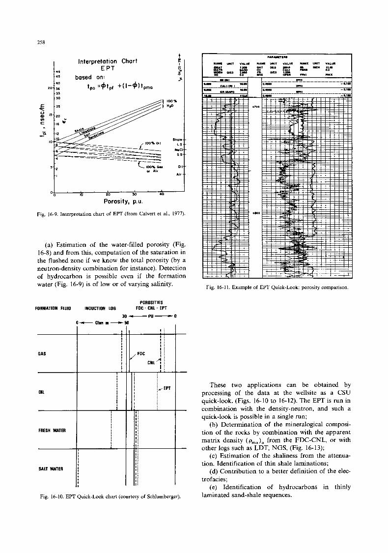
258
i
49
45
40
33 1 30 2 0 36
I i I : 1 : I .
I :
CNL? i
I i
FDC I
I !
- 1
GAS
OIL
FRESH WATER
SALT WATER
I nterpreta t ion Chart E PT
based on: t,, =+tpf +(I-+
I
I I I
I I
I I I
I I
I I
I
I
i I
I I
I
I I I
I I
I
I
1 I
I I I I I I I
100% Gaa Oi I 01 Air
Air
0 10 20 30 40
Porosity, p.u.
Fig. 16-9. Interpretation chart of EPT (from Calvert et al., 1977).
(a) Estimation of the water-filled porosity (Fig. 16-8) and from this, computation of the saturation in the flushed zone if we know the total porosity (by a neutron-density combination for instance). Detection of hydrocarbon is possible even if the formation water (Fig. 16-9) is of low or of varying salinity.
POROSITIES FORMATION FLUID INOUCTIOP! LOG FOC - CNL - EPT
30 - PU - 0 0- Ohm m -t
Fig. 16-10. EFT Quick-Look chart (courtesy of Schlumberger).
- 4700
Fig. 16-1 1. Example of EFT Quick-Look: porosity comparison.
These two applications can be obtained by processing of the data at the wellsite as a CSU quick-look. (Figs. 16- 10 to 16- 12). The EFT is run in combination with the density-neutron, and such a quick-look is possible in a single run;
(b) Determination of the mineralogical composi- tion of the rocks by combination with the apparent matrix density (p,,,,), from the FDC-CNL, or with other logs such as LDT, NGS, (Fig. 16-13);
(c) Estimation of the shaliness from the attenua- tion. Identification of thin shale laminations;
(d) Contribution to a better definition of the elec- trofacies;
(e) Identification of hydrocarbons in thinly laminated sand-shale sequences.
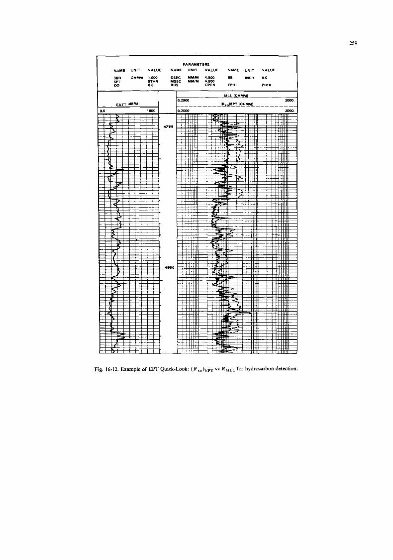
259
PARAMETERS
NAME UNIT VALUE NAME UNIT VALUE NAME UNIT VALUE
SBR OHMM 1.OOO DSEC MMlM 4.500 Bs INCH 0.0 SPT STAN MSEC MMlM 4.500 w 0.0 BHS OPEN FPHl PHlX
Fig. 16-12. Example of EPT Quick-Look: (R,,) , , , vs R,,, for hydrocarbon detection.
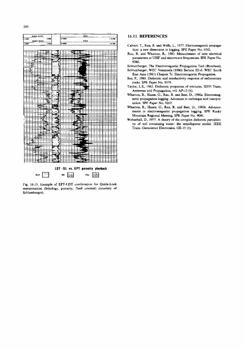
260
RHGA IGIC31 €PHI
YDu2 lGlC3l PHIA
......................... 2500 3 . m 0 4500 - 0.150
2 . m 3 . m 0.4500 - 0.160 ...............................................
RHGA IGIC31 €PHI
YDu2 lGlC3l PHIA
......................... 2500 3 . m 0 4500 - 0.150
2 . m 3 . m 0.4500 - 0.160 ...............................................
L O T - Q L vs. EPT porositg playback
all @ CIW snd
16.1 1 . REFERENCES
Calvert, T., Rau, R. and Wells, L., 1977. Electromagnetic propaga- tion: a new dimension in logging. SPE Paper No. 6542.
Rau, R. and Wharton, R., 1980. Measurement of core electrical parameters at UHF and microwave frequencies. SPE Paper No. 9380.
Schlumberger. The Electromagnetic Propagation Tool (Brochure). Schlumberger, WEC Venezuela (1980) Section 111-d. WEC South
East Asia (1981) Chapter 7c. Electromagnetic Propagation. Sen, P., 1980. Dielectric and conductivity response of sedimentary
rocks. SPE Paper No. 9379. Taylor, L.S., 1965. Dielectric properties of mixtures. IEEE Trans.
Antennae and Propagation, vol. AP- 13 (6). Wharton, R., Hazen, G., Rau, R. and Best, D., 1980a. Electromag-
netic propagation logging: Advances in technique and interpre- tation. SPE Paper No. 9267.
Wharton, R., Hazen, G., Rau, R. and Best, D., 1980b. Advance- ments in electromagnetic propagation logging. SPE Rocky Mountain Regional Meeting. SPE Paper No. 9041.
Wobschall, D., 1977. A theory of the complex dielectric permittiv- ity of soil containing water: the semidisperse model. IEEE Trans. Geoscience Electronics, GE-15 (1).
Fig. 16-13. Example of EFT-LDT combination for Quick-Look interpretation (lithology, porosity, fluid content) (courtesy of Schlumberger).
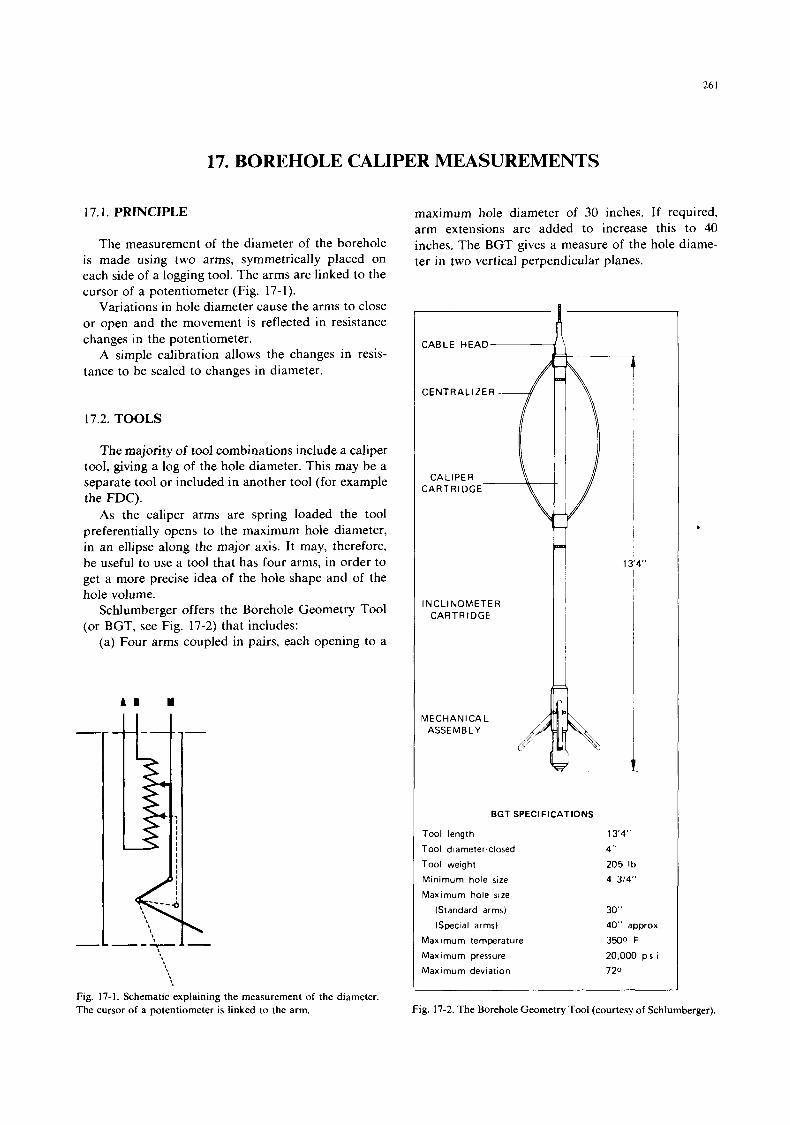
26 I
17. BOREHOLE CALIPER MEASUREMENTS
17.1. PRINCIPLE
The measurement of the diameter of the borehole is made using two arms, symmetrically placed on each side of a logging tool. The arms are linked to the cursor of a potentiometer (Fig. 17-1).
Variations in hole diameter cause the arms to close or open and the movement is reflected in resistance changes in the potentiometer.
A simple calibration allows the changes in resis- tance to be scaled to changes in diameter.
17.2. TOOLS
The majority of tool combinations include a caliper tool, giving a log of the hole diameter. This may be a separate tool or included in another tool (for example the FDC).
As the caliper arms are spring loaded the tool preferentially opens to the maximum hole diameter, in an ellipse along the major axis. It may, therefore, be useful to use a tool that has four arms, in order to get a more precise idea of the hole shape and of the hole volume.
Schlumberger offers the Borehole Geometry Tool (or BGT, see Fig. 17-2) that includes:
(a) Four arms coupled in pairs, each opening to a
A D I
_----
I
I I I I I
I I I I
Fig. 17-1. Schematic explaining the measurement of the diameter. The cursor of a potentiometer i s linked to the arm.
maximum hole diameter of 30 inches. If required, arm extensions are added to increase this to 40 inches. The BGT gives a measure of the hole diame- ter in two vertical perpendicular planes.
CENTRALIZER -
CALIPER CARTRIDGE-
INCLINOMETER CARTRIDGE
VlECH A N I CA L ASSEMBLY
CABLE HEAD
-
i
BGT SPECIFICATIONS
Tool length
Tool diameter closed
Tool weight
Minimum hole size
Maximum hole size
(Standard arms)
(Special arms)
Maximum temperature
Maximum pressure
Maximum deviation
I"
13'4"
4"
205 Ib
4 314"
30"
40" approx.
3500 F
20,000 ps I
720
Fig. 17-2. The Borehole Geometry Tool (courtesy of Schlumberger).
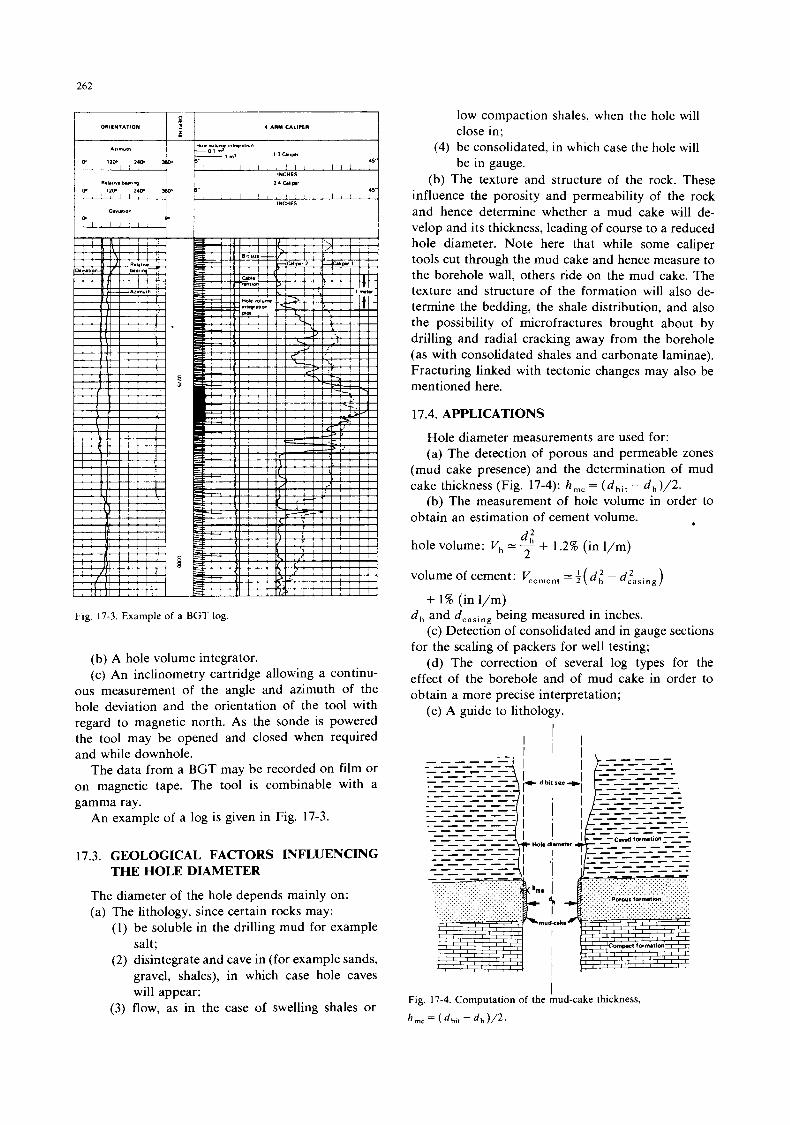
262
I I
Fig. 17-3. Example of a BGT log.
(b) A hole volume integrator. (c) An inclinometry cartridge allowing a continu-
ous measurement of the angle and azimuth of the hole deviation and the orientation of the tool with regard to magnetic north. As the sonde is powered the tool may be opened and closed when required and while downhole.
The data from a BGT may be recorded on film or on magnetic tape. The tool is combinable with a gamma ray.
An example of a log is gven in Fig. 17-3.
17.3. GEOLOGICAL FACTORS INFLUENCING THE HOLE DIAMETER
The diameter of the hole depends mainly on: (a) The lithology, since certain rocks may:
(1) be soluble in the drilling mud for example salt;
(2) disintegrate and cave in (for example sands, gravel, shales), in which case hole caves will appear;
(3) flow, as in the case of swelling shales or
low compaction shales, when the hole will close in;
(4) be consolidated, in which case the hole will be in gauge.
(b) The texture and structure of the rock. These influence the porosity and permeability of the rock and hence determine whether a mud cake will de- velop and its thickness, leading of course to a reduced hole diameter. Note here that while some caliper tools cut through the mud cake and hence measure to the borehole wall, others ride on the mud cake. The texture and structure of the formation will also de- termine the bedding, the shale distribution, and also the possibility of microfractures brought about by drilling and radial cracking away from the borehole (as with consolidated shales and carbonate laminae). Fracturing linked with tectonic changes may also be mentioned here.
17.4. APPLICATIONS
Hole diameter measurements are used for: (a) The detection of porous and permeable zones
(mud cake presence) and the determination of mud cake thickness (Fig. 17-4): h,, = (dbit - d h ) / 2 .
(b) The measurement of hole volume in order to obtain an estimation of cement volume.
hole volume: Vh 2: - + 1.2% (in l/m) 2 volume of cement: K ~ ~ ~ ~ , = +( df - dzasing)
+ 1 % (in I/m) d, and dcasing being measured in inches.
(c) Detection of consolidated and in gauge sections for the scaling of packers for well testing;
(d) The correction of several log types for the effect of the borehole and of mud cake in order to obtain a more precise interpretation;
* d f
(e) A guide to lithology. I
I Fig. 17-4. Computation of the mud-cake thickness,
h mc = ( d b , , - d , )/2.
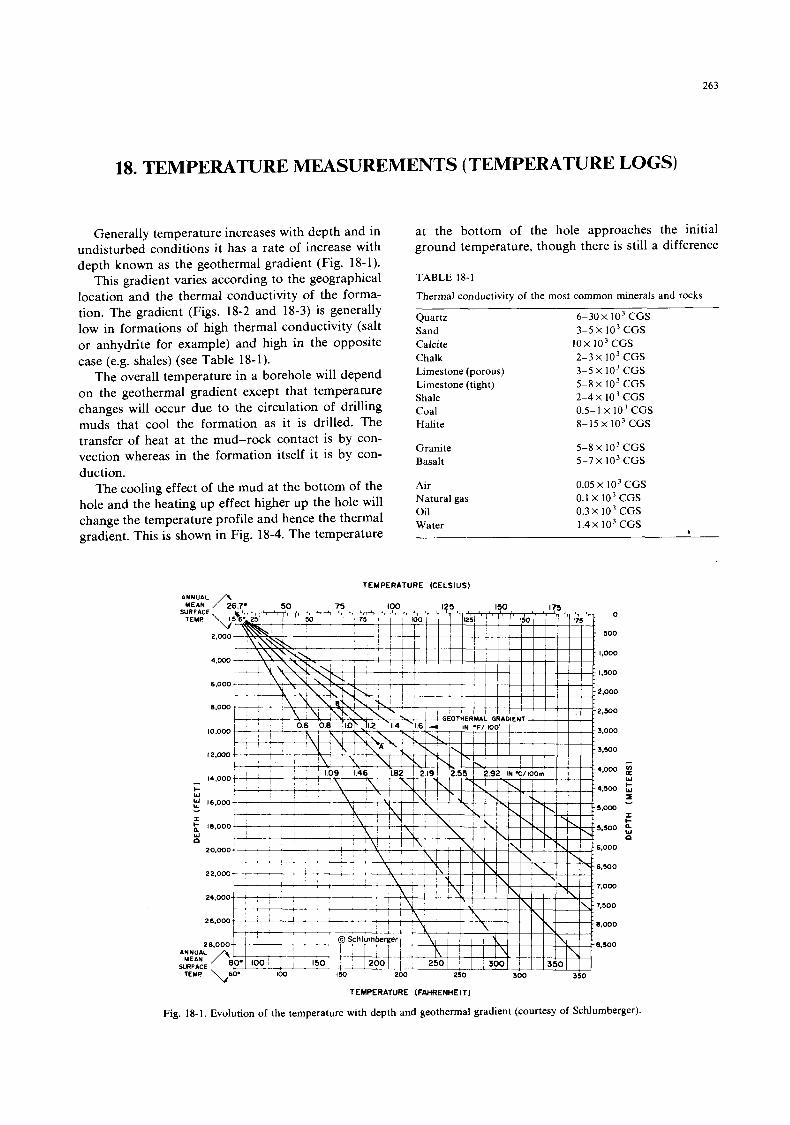
263
18. TEMPERATURE MEASUREMENTS (TEMPERATURE LOGS)
Generally temperature increases with depth and in undisturbed conditions it has a rate of increase with depth known as the geothermal gradient (Fig. 18-1).
T h s gradient varies according to the geographical location and the thermal conductivity of the forma- tion. The gradient (Figs. 18-2 and 18-3) is generally low in formations of high thermal conductivity (salt or anhydrite for example) and hgh in the opposite case (e.g. shales) (see Table 18-1).
The overall temperature in a borehole will depend on the geothermal gradient except that temperature changes will occur due to the circulation of drilling muds that cool the formation as it is drilled. The transfer of heat at the mud-rock contact is by con- vection whereas in the formation itself it is by con- duction.
The cooling effect of the mud at the bottom of the hole and the heating up effect higher up the hole will change the temperature profile and hence the thermal gradient. This is shown in Fig. 18-4. The temperature
at the bottom of the hole approaches the initial ground temperature, though there is still a difference
TABLE 18-1
Thermal conductivity of the most common minerals and rocks
Quartz 6-30 x lo3 CGS Sand 3-5 X lo3 CGS
Chalk 2-3 x lo3 CGS Limestone (porous) 3-5X lo3 CGS Limestone (tight) 5-8 X lo3 CGS Shale 2-4X lo3 CGS Coal 0.5-1 x lo3 CGS Halite 8-15 x lo3 CGS
Calcite I O X 103 CGS
Granite Basalt
Air Natural gas Oil Water
5-8 X lo3 CGS 5-7 X lo3 CGS
0.05 X lo3 CGS 0.1 X lo3 CGS 0.3 X lo3 CGS 1.4X lo3 CGS
TEMPERATURE (CELSIUS) ANNUAL A
0
500
1,000
I, 500
2.000
2,500
3,000
3.500
4.000 2 W
- 4.500 t;
I
I
- 5,000
5,500 n
6,000
6,500
7,000
7.500
8.000
8.500
TEMPERATURE (FAHRENHEIT)
Fig. 18-1. Evolution of the temperature with depth and geothermal gradient (courtesy of Schlumberger).
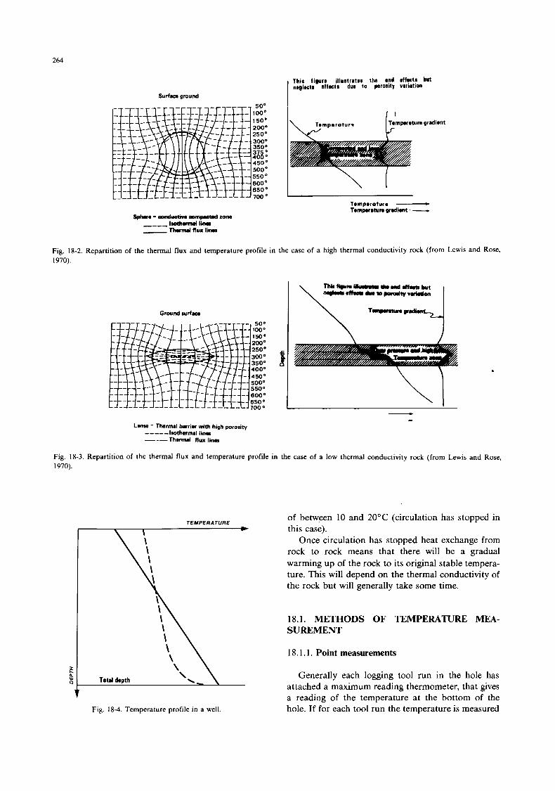
264
50' 1000 150' 2000
- 250' - 300° - 350:
375 400' 450' 500°
600 a 850'
- 550'
- 700
Surface ground
Tamparatun gradient
This figure illustrates the end off?ct! but nqlwtr affects dun to porosaly variation
Fig. 18-2. Repartition of the thermal flux and temperature profile in the case of a high thermal conductivity rock (from Lewis and Rose, 1970).
Ground rurfrcr
L ~ M = Thermal barrier with high porosity -----lrotharmJ l i n r ---Th.rmal flux l ina
Fig. 18-3. Repartition of the thermal flux and temperature profile in the case of a low thermal conductivity rock (from Lewis and Rose, 1970).
t Fig. 18-4. Temperature profile in a well.
of between 10 and 20°C (circulation has stopped in this case).
Once circulation has stopped heat exchange from rock to rock means that there will be a gradual warming up of the rock to its original stable tempera- ture. This will depend on the thermal conductivity of the rock but will generally take some time.
18.1. METHODS OF TEMPERATURE MEA- SUREMENT
18.1.1. Point measurements
Generally each logging tool run in the hole has attached a maximum reading thermometer, that gives a reading of the temperature at the bottom of the hole. If for each tool run the temperature is measured
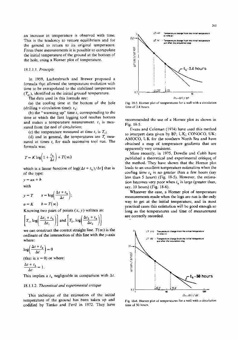
265
an increase in temperature is observed with time. This is the tendency to restore equilibrium and for the ground to return to its original temperature. From these measurements it is possible to extrapolate the initial temperature of the ground at the bottom of the hole, using a Horner plot of temperature.
1 8.1.1.1. Principle
In 1959, Lachenbruch and Brewer proposed a formula t h p allowed the temperature evolution with time to be extrapolated to the stabilised temperature ( Tm), identified as the initial ground temperature.
The data used in t h s formula are: (a) the cooling time at the bottom of the hole
(drilling + circulation time): tk; (b) the “warming up” time t , corresponding to the
time at which the first logging tool reaches bottom and makes a temperature measurement. t , is mea- sured from the end of circulation;
(c) the temperature measured at time t , is TI; (d) and in general, the temperatures are mea-
sured at times t , for each successive tool run. The formula was:
T = Klog( 1 +$) + T(m)
which is a linear function of log[(At + tk)/At] that is of the type: y = a x + b with
y = T x = b g ( - ‘k ) . 7
a = K b=T(oo) Knowing two pairs of points (x, y ) written as:
we can construct the correct straight line. T( 00) is the ordinate of the intersection of this line with the y-axis where: log( +) A t + t = 0
(that is x = 0) or where: At + t,
A t -- - 1.
This implies a t , negligeable in comparison with At.
18.1.1.2. Theoretical and experimental critique
This technique of the estimation of the initial temperature of the ground has been taken up and codified by Timko and Fertl in 1972. They have
( t k + A t ) / A f
Fig. 18-5. Horner plot of temperatures for a well with a circulation time of 2.4 hours.
recommended the use of a Horner plot as shown in Fig. 18-5.
Evans and Coleman (1974) have used this method to interpret data given by BP, UK; CONOCO, UK; AMOCO, UK for the southern North Sea and have obtained a map of temperature gradients that are apparently very consistent.
More recently, in 1975, Dowdle and Cobb have published a theoretical and experimental critiquq of the method. They have shown that the Horner plot leads to an excellent temperature estimation when the cooling time t , is no greater than a few hours (say less than 5 hours) (Fig. 18-5). However, the estima- tion becomes very poor when t , is large (greater than, say, 10 hours) (Fig. 18-6).
Whatever the case, a Homer plot of temperature measurements made when the logs are run is the only way to get at the initial temperature, and in most practical cases this estimation will be good enough so long as the temperatures and time of measurement are correctly recorded.
A T ( A t ) - Temperature change from the !nttbal temmrature at h m A t
A T (0) - Tsmpaature change from the mnul tempnhrre lust after the cumhtmn stop
11-
- 0
Q
..- h
h c Q L 0
-
I
loo 0.7
10
(tk+ A t ) / A t
Fig. 18-6. Homer plot of temperatures for a well with a circulation time of 50 hours.
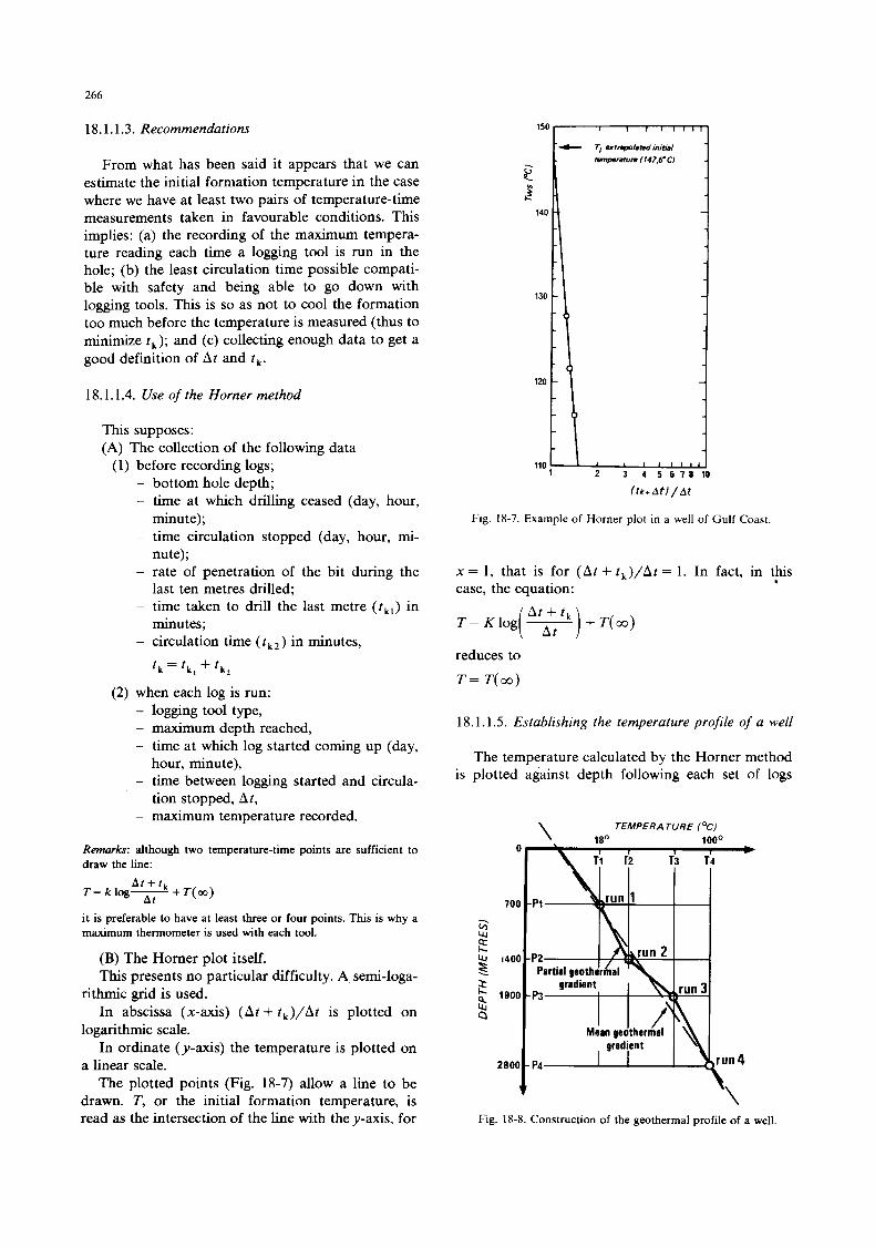
266
18.1.1.3. Recommendations
From what has been said it appears that we can estimate the initial formation temperature in the case where we have at least two pairs of temperature-time measurements taken in favourable conditions. This implies: (a) the recording of the maximum tempera- ture reading each time a logging tool is run in the hole; (b) the least circulation time possible compati- ble with safety and being able to go down with logging tools. T h s is so as not to cool the formation too much before the temperature is measured (thus to minimize t k ) ; and (c) collecting enough data to get a good definition of At and tk.
18.1.1.4. Use of the Horner method
This supposes: (A) The collection of the following data
(1) before recording logs; - bottom hole depth; - time at which drilling ceased (day, hour,
- time circulation stopped (day, hour, mi-
- rate of penetration of the bit during the
- time taken to drill the last metre ( t k , ) in
- circulation time ( t k 2 ) in minutes,
minute);
nute);
last ten metres drilled;
minutes;
l k = t k l + ‘ k 2
(2) when each log is run: - logging tool type, - maximum depth reached, - time at which log started coming up (day,
- time between logging started and circula-
- maximum temperature recorded.
hour, minute),
tion stopped, A t ,
Remarks: although two temperature-time points are sufficient to draw the line:
A t + t k T = k l o g - A t + T ( o o )
it is preferable to have at least three or four points. This is why a maximum thermometer is used with each tool.
(B) The Horner plot itself. This presents no particular difficulty. A semi-loga-
rithmic grid is used. In abscissa (x-axis) (A t + t k ) / A t is plotted on
logarithmic scale. In ordinate (y-axis) the temperature is plotted on
a linear scale. The plotted points (Fig. 18-7) allow a line to be
drawn. T, or the initial formation temperature, is read as the intersection of the line with the y-axis. for
120 I\ 110
2 3 4 5 6 7 8 1 0 1
( t k + A t ) / A t
Fig. 18-7. Example of Horner plot in a well of Gulf Coast.
x = 1, that is for ( A t + t k ) / A t = 1. In fact, in this case, the equation: e
At + t , T = K log( T ) + T( CO )
reduces to T = T ( w )
18.1.1.5. Establishing the temperature profile of a well
The temperature calculated by the Horner method is plotted against depth following each set of logs
Fig. 18-8. Construction of the geothermal profile of a well.
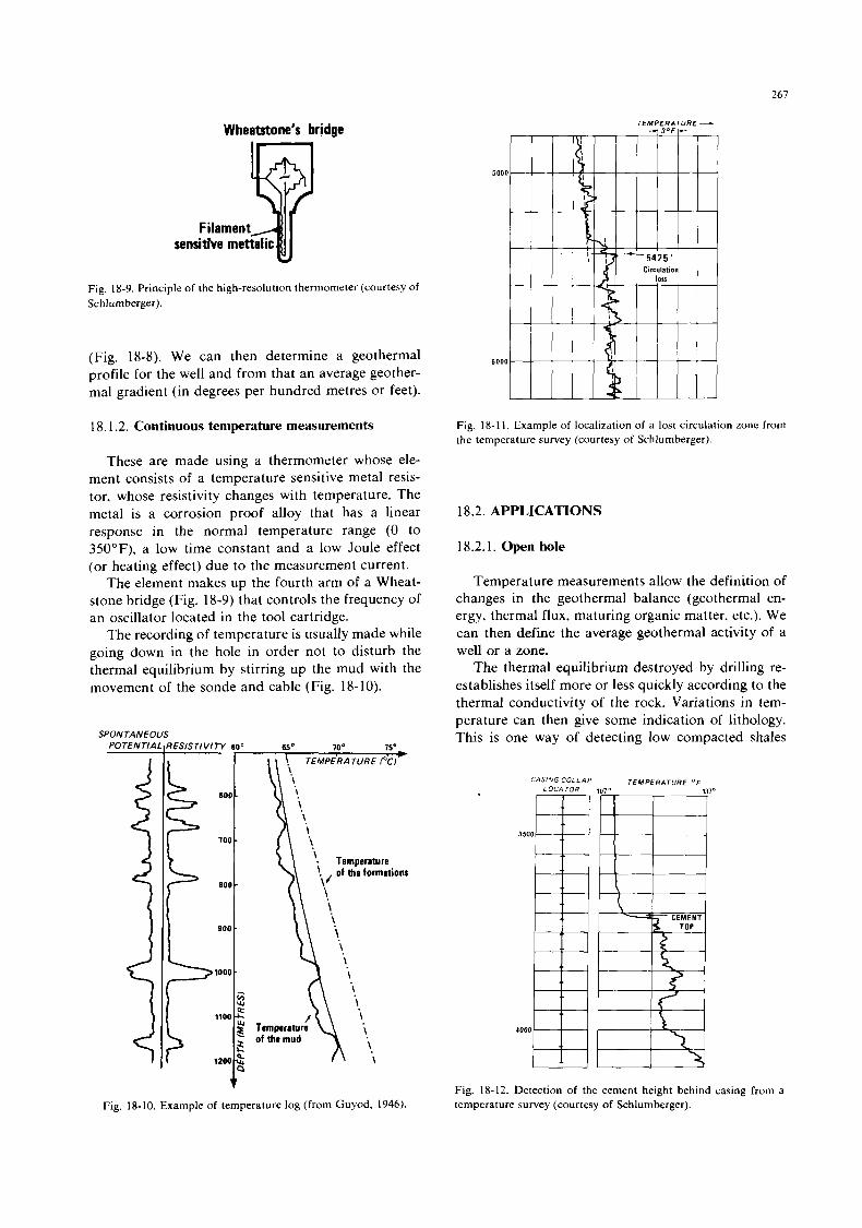
Wheatstone's bridge
261
T E M P E R A T U R E - i 1 O F C
Filament
Fig. 18-9. Principle of the high-resolution thermometer (courtesy of Schl umberger).
(Fig. 18-8). We can then determine a geothermal profile for the well and from that an average geother- mal gradient (in degrees per hundred metres or feet).
18.1.2. Continuous temperature measurements
These are made using a thermometer whose ele- ment consists of a temperature sensitive metal resis- tor, whose resistivity changes with temperature. The metal is a corrosion proof alloy that has a linear response in the normal temperature range (0 to 350"F), a low time constant and a low Joule effect (or heating effect) due to the measurement current.
The element makes up the fourth arm of a Wheat- stone bridge (Fig. 18-9) that controls the frequency of an oscillator located in the tool cartridge.
The recording of temperature is usually made while going down in the hole in order not to disturb the thermal equilibrium by stirring up the mud with the movement of the sonde and cable (Fig. 18-10).
SPONTANEOUS POTEN TIA
Fig. 18-10. Example of temperature log (from Guyod, 1946).
Fig. 18- 1 I . Example of localization of a lost circulation zone from the temperature survey (courtesy of Schlumberger).
18.2. APPLICATIONS
18.2.1. Open hole
Temperature measurements allow the definition of changes in the geothermal balance (geothermal en- ergy, thermal flux, maturing organic matter, etc.). We can then define the average geothermal activity of a well or a zone.
The thermal equilibrium destroyed by drilling re- establishes itself more or less quickly according to the thermal conductivity of the rock. Variations in tem- perature can then give some indication of lithology. This is one way of detecting low compacted shales
CASING C O L L A R TEMPERATURE OF
3500
4000
Fig. 18-12. Detection of the cement height behind casing from a temperature survey (courtesy of Schlumberger).
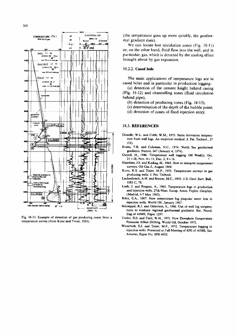
268
ELECTRICAL LOG
ohms. rn /WdI full of 0aO ! lo I Normal G I Normil
TEMPERATURE ( O F . )
I100 -
I200 -
IUO -
I u o -
IW -
U O ) -
L- RESISTIVITY -I (onrns - rnr
Fig. 18-13. Example of detection of gas producing zones from a temperature survey (from Kunz and Tixier, 1955).
(the temperature goes up more quickly, the geother- mal gradient rises).
We can locate lost circulation zones (Fig. 18-1 I ) or, on the other hand, fluid flow into the well, and in particular, gas, which is detected by the cooling effect brought about by gas expansion.
18.2.2. Cased hole
The main applications of temperature logs are in cased holes and in particular in production logging:
(a) detection of the cement height behind casing (Fig. 18- 12) and channelling zones (fluid circulation behind pipe);
(b) detection of producing zones (Fig. 18-13); (c) determination of the depth of the bubble point; (d) detection of zones of fluid injection entry.
18.3. REFERENCES
Dowdle, W.L. and Cobb, W.M., 1975. Static formation tempera- ture from well logs. An empirical method. J. Pet. Technol., 27 (1 1).
Evans, T.R. and Coleman, N.C., 1974. North Sea geothermal gradients. Nature, 247 (January 4, 1974).
Guyod, H., 1946. Temperature well logging. Oil Weekly, Oct. 21 +28, Nov. 4+ 11, Dec. 2, 9+ 16.
Hutchins, J.S. and Kading, H., 1969. How to interpret temperature surveys. Oil Gas J., August 1969.
Kunz, K.S. and Tixier, M.P., 1955. Temperature surveys in gas producing wells. J. Pet. Technol.
Lachenbruch, A.H. and Brewer, M.C., 1959. U.S. Geol. Surv. Bull., 1083 C, 78.
h b , J. and Poupon, A., 1965. Temperature logs in production and injection wells. 27th Meet. Europ. Assoc. Explor. Geophys. (Madrid, 5-7 May 1965).
Riley, E.A., 1%7. New temperature log pinpoint water loss in injection wells. World Oil, January 1967.
Schoeppel, R.J. and Gilarranz, S., 1966. Use of well log tempera- tures to evaluate regional geothermal gradients. Soc. Petrol. Eng of AIME, Paper 1297.
Timko, D.J. and F e d , W.H., 1972. How Downhole Temperature Pressures Affect Drilling. World Oil, October 1972.
Witterholt, E.J. and Tixier, M.P., 1972. Temperature logging in injection wells. Presented at Fall Meeting of SPE of AIME, San Antonio, Paper No. SPE 4022.
.
269
19. DIP MEASUREMENTS (DIPMETER LOGS)
19.1. OBJECTIVE
The aim of this log is to determine the angle to the horizontal and the azimuth referenced to magnetic north and geographcal north of the dip of the planes cut by the well. These planes can be -bed boundarjes; -an open or closed fracture; -an erosional surface; -a stylolitic joint.. . The planes can be planar, or can correspond to a convex or concave surface intersecting the well.
19.2. PRINCIPLE
A plane is defined by a minimum of three points not lying in a straight line. It should be sufficient, therefore, to know the coordinates ( X , Y, Z ) of three points in space to define the plane. These three points will be the intersection of three generatrices of the borehole wall with the plane (Fig. 19-1).
19.3. THE MEASUREMENT PROCESS (Fig. 19-2)
The tool consists of .at least three electrodes‘’) mounted on pads in a plane perpendicular to the axis
MAGNETIC NORTH \
HOLE AXIS
Fig. 19-1. A plane is defined by a minimum of three points not lying on a straight line. The three points are the intersection of three generatrices of the borehole wall with the plane (i.e. bed boundary).
of the tool and situated at angles of 120 degrees (3-pad tool) or 90 degrees (4-pad tool) to each other.
The three electrodes each make a resistivity mea- surement of the borehole wall. Because of the size of the electrode and the current focusing that occurs on each pad the resistivity measurement is assumed to be a point measurement at the electrode. When the tool crosses the boundary between two formations the corresponding response change is recorded for each pad at different depths according to the ap- parent dip (that is to say in relation to the borehole axis). The relative depth differences for the curves give the necessary information to evaluate the dip and the azimuth if we also know:
(a) the orientation of the sonde defined by the azimuth and one of the pads (pad number 1). This azimuth is the angle formed by the horizontal projec- tion of the lines perpendicular to the sonde axis and passing through pad number 1 and magnetic north;
(b) the borehole deviation and its azimuth; (c) the hole diameter (or more exactly the distahce
between the sonde and each pad). The azimuth of pad 1 with respect to magnetic
north is measured using a compass to which is fixed the cursor of a potentiometer. The movement of the compass pointer is reflected in changes in the poten- tiometer resistance. The borehole deviation is mea- sured using a pendulum linked to a potentiometer whose resistance varies as a function of the deviation.
The azimuth of the deviation is measured by means of another pendulum that is continuously aligned in a vertical plane passing through the low side of the borehole. This pendulum is linked to a circular potentiometer whose resistance is a function of the angle formed by the azimuth of the deviation and of the ’azimuth of pad number 1 as reference (called the relative bearing).
Finally the hole diameter is measured using potentiometers linked to the sideways movement of the pads.
19.4. DIPMETER TOOLS * 19.4.1. Discontinuous dipmeters
19.4.1.1. Anisotropy dipmeter
We can mention as a reference the “anisotropy dipmeter”, used by Schlumberger around 1936 and
(1) Nuclear or acoustic dipmeters do not exist until now. * The toools described are those of Schlumberger.
270
Onentat,on o f the deviation (rela twe bearing)
DeviarJon angle of the ho for drift angle)
AzM 7 ,l’)
Magnetic Norrh
/ Compass
Correlation curves
I Rests tivi ry measurements
(4 Dads)
.
Fig. 19-2. Principle of the dipmeter showing the different measurements made by the tool (from Dresser-Atlas document).
which measured the difference in potential between two electrodes situated on axes at 90”. The orienta- tion of the sonde and the borehole deviation were given by an induction compass. T h s method used the anisotropy property of shales.
i 9.4.1.2. SP dipmeter
Towards 1942, Schlumberger introduced to the market a three pad dipmeter, recording SP curves. A photoclinometer associated with the tool gave the orientation of electrode number 1 referenced to mag- netic north as well as the deviation and azimuth of the well, in the form of a negative taken with the sonde stopped.
19.4.1.3. Lateral dipmeter
In 1945 the recording of SP curves was abandoned in favour of small “lateral” systems since the SP often had little character in salt muds or in front of very resistive formations.
19.4.2. Continuous dipmeters
19.4.2.1. CDM (Continuous dipmeter)
In 1952, Schlumberger put into service a continu- ous dipmeter (Fig. 19-3) that allowed the continuous recording of three parameters: the deviation and azimuth of the well and the orientation of electrode number 1; thanks to a system that transmitted to the surface the information recorded by each potentiom- eter.
At the same time there were changes in the pad curves. First pads of a microlog and then, later, of a focussed micro-device were used, with the pad ap- plied to the formation by means of articulated arms (1956). According to the CDM type, hole diameters of between 4 and 19 inches could be logged.
The calculation of dips consisted first in establish- ing correlations between the three curves, noting the displacement by superposition of the curves, and
- then in defining the angle and azimuth of the dip knowing the angle and azimuth of the hole deviation.
27 1
Fig. 19-3. Three-pad dipmeter (CDM) (courtesy of Schlumberger).
Although well developed, this method presented some problems:
(a) In holes that are caved or ovalized one of the pads may not touch the wall of the hole (floating pad) and the recorded resistivity would be about equal to the mud resistivity so giving a characterless curve. The calculation of dip becomes impossible since only two points are known. In some cases to get over this problem the log may be recorded twice in the hope that the sonde will turn and the pads take a different path.
(b) In very deviated wells, the tool presses against one side of the hole under its own weight, leading to a possible partial or complete closing of the sonde. The uppermost pad is likely to be free of the wall and so gives a characterless curve.
(c) In the case of very saline muds the resistivity curves will also be lacking in character and hence the correlations difficult or imprecise.
(d) In the case of oil base muds a film of oil comes between the pad and the formation and no current
B A
Fig. 19-4. a. Photograph of the HDT tool (courtesy of Schlum- berger).
b
N,!
I
I I
/ nOr12oniai I / Fig. 19-4. b. Principle of the HDT dip measurement (courtesy of
passes. Special pads called “scratcher pads” are avail- - Schlumberger).
212
able to get over this. The results are often erratic as the pad's contact is very irregular as the tool moves in the hole.
(e) As already described above the correlations had to be established manually. The interpretation, itself a manual process for a long time, is now done on a computer.
Figure 19-8 shows a field example of a dipmeter log recorded with a CDM type tool. Remark: The Dresser Atlas CDM had the advantage of having moveable pads that were free to rotate by + 15' about a vertical axis at the arm end, so improving the pad contact with the wall.
ELECTIIKAL CUllRENT EMITTED BY THE SONIW, A N 0 THE ELECTROOOCS
I INSULATED RAT-
1 1
i \
71
19.4.2.2. HDT (High resolution dipmeter tool: Fig. 19-4)
Since 1967 a four-pad dipmeter has almost totally replaced the CDM (Fig. 19-4 a and b).
(a) The sonde is powered and can be opened and closed at will from the surface.
(b) It has four pads at 90" to each other. This means that if one pad does not touch the borehole wall because the hole is ovalized or the hole is devia- ted (floating pad) then three pads can still give good logs that allow the determination of dip planes.
ELECTRONICS ' ACOUlSlTlON AN0 TRANSMISSION --- OF DATA FROM INCLINOMETER AND ELECTRODES
\ \
/ / ' / / , SON3E (4 PADS) BOREHOLE DIAMETER
' EACH ELEtTRoM MEASURES A ll< CURRENT DISPLAYED HERE AS CWIVE
CORRELATION RELATIVE POSITION SHIFTS
BETWEEN CURRENT CURVES
Fig. 19-5. The different measurements of the SHDT (courtesy of Schlumberger).
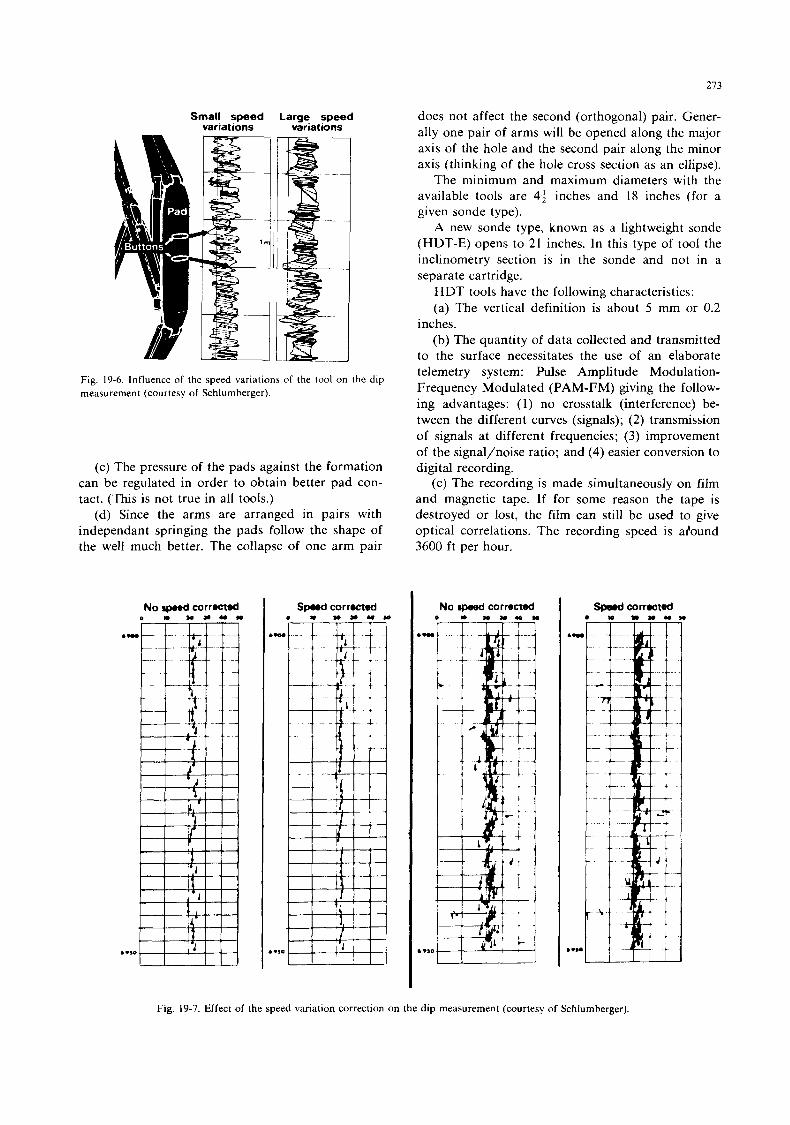
273
Small Speed Large speed variations variations
Fig. 19-6. Influence of the speed variations of the tool on the dip measurement (courtesy of Schlumberger).
(c) The pressure of the pads against the formation can be regulated in order to obtain better pad con- tact. (This is not true in all tools.)
(d) Since the arms are arranged in pairs with independant springing the pads follow the shape of the well much better. The collapse of one arm pair
No speed corrected 0 m a 0 a e u I e
S p m i corrocted 0 m Y W
b W
. -30
does not affect the second (orthogonal) pair. Gener- ally one pair of arms will be opened along the major axis of the hole and the second pair along the minor axis (thinking of the hole cross section as an ellipse).
The minimum and maximum diameters with the available tools are 44 inches and 18 inches (for a given sonde type).
A new sonde type, known as a lightweight sonde (HDT-E) opens to 21 inches. In this type of tool the inclinometry section is in the sonde and not in a separate cartridge.
HDT tools have the following characteristics: (a) The vertical definition is about 5 mm or 0.2
inches. (b) The quantity of data collected and transmitted
to the surface necessitates the use of an elaborate telemetry system: Pulse Amplitude Modulation- Frequency Modulated (PAM-FM) giving the follow- ing advantages: (1) no crosstalk (interference) be- tween the different curves (signals); (2) transmission of signals at different frequencies; (3) improvement of the signal/noise ratio; and (4) easier conversion to digital recording.
(c) The recording is made simultaneously on film and magnetic tape. If for some reason the tape is destroyed or lost, the film can still be used to give optical correlations. The recording speed is afound 3600 f t per hour.
No speed corracted 0 - Y Y . 0
Sped mrrocted H m n u .... D
Fig. 19-7. Effect of the speed variation correction on the dip measurement (courtesy of Schlumberger).
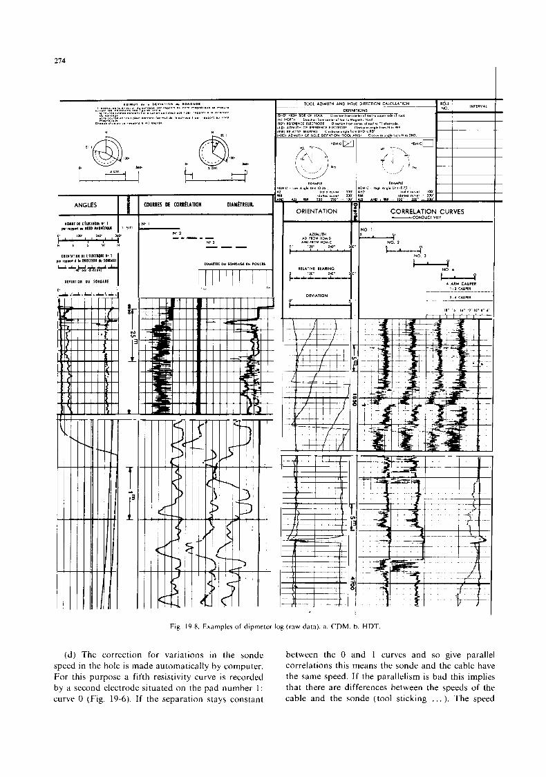
214
1 COUUBES DE COUR~LATION DIAML~UEU~,
I , 6.
Fig. 19-8. Examples of dipmeter
**D FROM "DM c
RELATIVE BEARING 0 l W ' 140" +ILLLLLI
rn c
I
log (raw data) a CDM b
CORRELATION CURVES -CONDUCTIVITY
3 1
P NO 2
L L - 4 N O 3
H DT
(d) The correction for variations in the sonde between the 0 and 1 curves and so give parallel correlations this means the sonde and the cable have the same speed. If the parallelism is bad this implies that there are differences between the speeds of the cable and the sonde (tool sticking . . . ). The speed
speed in the hole is made automatically by computer. For this purpose a fifth resistivity curve is recorded by a second electrode situated on the pad number 1: curve 0 (Fig. 19-6). If the separation stays constant
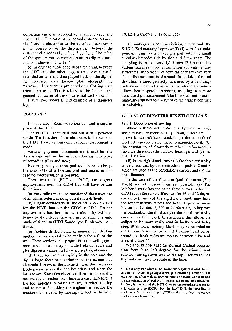
275
correction curve is recorded on magnetic tape and not on film. The ratio of the actual distance between the 0 and 1 electrodes to the calculated separation allows correction of the displacement between the different electrodes (h,.*, h,. , , h,.,, h 4 . , ) . The effect of the speed variation correction on the dip measure- ments is shown in Fig. 19-7.
(e) In order to allow good depth matching between the HDT and the other logs, a resistivity curve is recorded on tape and then played back on the dipme- ter processed data (arrow plot) alongside the “arrows”. This curve is presented on a floating scale (that is no scale). This is related to the fact that the geometrical factor of the sonde is not well known.
Figure 19-8 shows a field example of a dipmeter log.
19.4.2.3. PDT
In some areas (South America) this tool is used in place of the HDT.
The PDT is a three-pad tool but with a powered sonde. The focusing of the electrodes is the same as the HDT. However, only one caliper measurement is made.
An analog system of transmission is used but the data is digitized on the surface, allowing both types of recording (film and tape).
Evidently being a three-pad tool there is always the possibility of a floating pad and again, in this case no interpretation is possible.
These two tools (PDT and HDT) are a great improvement over the CDM but still have certain limitations:
(a) Very saline muds: as mentioned the curves are often characterless, making correlation difficult.
(b) Highly deviated wells: the effect is less marked for the HDT than for the CDM or PDT. Further improvement has been brought about by Schlum- berger by the introduction and use of a lighter sonde made of titanium (HDT Sonde type F) already men- tioned.
(c) Turbine drilled holes: in general this drilling method causes a spiral to be cut into the wall of the well. These sections that project into the well appear more resistant and may simulate beds or layers and give dipmeter values that have no real significance.
(d) If the tool rotates rapidly in the hole and the dip is large there is a variation of the azimuth of electrode 1 between the nloment when the first elec- trode passes across the bed boundary and when the last crosses. Since this effect is difficult to detect it is not usually corrected for. There is a case therefore, if the tool appears to rotate rapidly, to refuse the log and to repeat it, asking the engineer to reduce the tension on the cable by moving the tool in the hole.
19.4.2.4. SHDT (Fig. 19-5, p. 272)
Schlumberger is commercializing a new tool, the SHDT (Sedimentary Dipmeter Tool) with four inde- pendant arms, each carrying a pad with two small circular electrodes side by side and 3 cm apart. The sampling is made every 1/10 inch (2.5 mm). Ths system acquires more information on sedimentary structures: lithological or textural changes over very short distances can be detected. In addition the tool deviation is more precisely measured by a new mag- netometer. The tool also has an accelerometer whch allows better speed corrections, resulting in a more accurate dip measurement. The Emex current is auto- matically adjusted to always have the highest contrast in resistivity.
19.5. USE OF DIPMETER RESISTIVITY LOGS
19.5.1. Description of raw log Where a three-pad continuous dipmeter is used,
seven curves are recorded (Fig. 19-8a). These are: (A) In the left-hand track *: (a) the azimuth of
electrode number 1 referenced to magnetic north; (b) the orientation of electrode number 1 referenced to the hole direction (the relative bearing); and (c) the hole deviation. *
(B) In the right-hand track: (a) the three resistivity curves, recorded by the electrodes on pads 1, 2 and 3 which are used as the correlations curves; and (b) the hole diameter.
In the case of the four-arm (pad) dipmeter (Fig. 19-8b) several presentations are possible: (a) The left-hand track has the same three curves as for the CDM (with the same differences for 36 and 72 degree cartridges); and (b) the right-hand track may have the four resistivity curves and both calipers or possi- bly on the l/lOOO, 1/500 or 1/200 scale, to improve the readability, the third and/or the fourth resistivity curves may be left off. In particular, this allows the caliper to be more easily read in badly caved holes (Fig. 19-8b lower section). Marks may be recorded on certain curves (deviation and 2-4 caliper) and corre- spond to depth reference points between film and magnetic tape * * .
We should note that the normal gradual progres- sion from 0 to 360 degrees for the azimuth and relative bearing curves end with a rapid return to 0 as the tool continues to rotate in the hole.
* This is only true when a 36” inclinometry system is used. In the case of 72” system, high angle cartridge, a recording is made of: (a) the direction of the well directly referenced to magnetic north; and (b) the orientation of pad No. I referenced to the hole direction. ** Only in the case of the HDT-C where the recording is made as a function of time (DDR). For the HDT-D/E the recording is made as a function of depth (‘lTR) and so no depth reference marks are made on film.
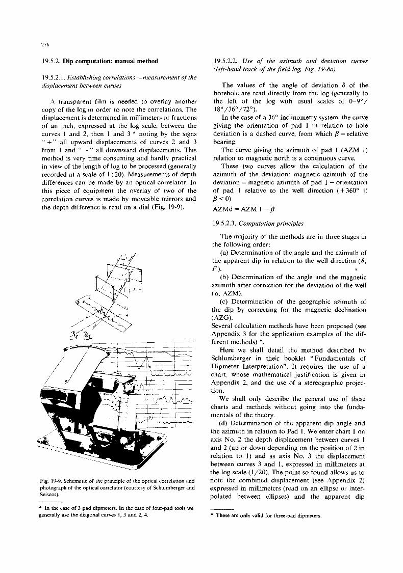
216
19.5.2. Dip computation: manual method
19.5.2.1. Establishing correlations-measurement ofthe displacement between curves
A transparent film is needed to overlay another copy of the log in order to note the correlations. The displacement is determined in millimeters or fractions of an inch, expressed at the log scale, between the curves 1 and 2, then 1 and 3 * noting by the signs '' +" all upward displacements of curves 2 and 3 from I and " -" all downward displacements. This method is very time consuming and hardly practical in view of the length of log to be processed (generally recorded at a scale of 1 : 20). Measurements of depth differences can be made by an optical correlator. In this piece of equipment the overlay of two of the correlation curves is made by moveable mirrors and the depth difference is read on a dial (Fig. 19-9).
Fig. 19-9. Schematic of the principle of the optical correlation and photograph of the optical correlator (courtesy of Schlumberger and Seiscor).
19.5.2.2. Use of the azimuth and deviation curves (left-hand track of the field log, Fig. 19-8a)
The values of the angle of deviation 6 of the borehole are read directly from the log (generally to the left of the log with usual scales of 0-9O/ 18"/36"/72").
In the case of a 36" inclinometry system, the curve giving the orientation of pad 1 in relation to hole deviation is a dashed curve, from which P = relative bearing.
The curve giving the azimuth of pad 1 (AZM 1) relation to magnetic north is a continuous curve.
These two curves allow the calculation of the azimuth of the deviation: magnetic azimuth of the deviation = magnetic azimuth of pad 1 - orientation of pad 1 relative to the well direction (+360" if P < 0) AZMd = AZM 1 - P
19.5.2.3. Computation principles
The majority of the methods are in three stages in the following order:
(a) Determination of the angle and the azimuth of the apparent dip in relation to the well direction (0, F ) . 4
(b) Determination of the angle and the magnetic azimuth after correction for the deviation of the well (a, AZM).
(c) Determination of the geographic azimuth of the dip by correcting for the magnetic declination (AZG). Several calculation methods have been proposed (see Appendix 3 for the application examples of the dif- ferent methods) *.
Here we shall detail the method described by Schlumberger in their booklet "Fundamentals of Dipmeter Interpretation". It requires the use of a chart, whose mathematical justification is given in Appendix 2, and the use of a stereographic projec- tion.
We shall only describe the general use of these charts and methods without going into the funda- mentals of the theory.
(d) Determination of the apparent dip angle and the azimuth in relation to Pad 1. We enter chart 1 on axis No. 2 the depth displacement between curves 1 and 2 (up or down depending on the position of 2 in relation to 1) and as axis No. 3 the displacement between curves 3 and 1, expressed in millimeters at the log scale (1/20). The point so found allows us to note the combined displacement (see Appendix 2) expressed in millimeters (read on an ellipse or inter- polated between ellipses) and the apparent dip
* In the case of 3 pad dipmeters. In the case of four-pad tools we generally use the diagonal curves 1, 3 and 2,4. * These are only valid for three-pad dipmeters.
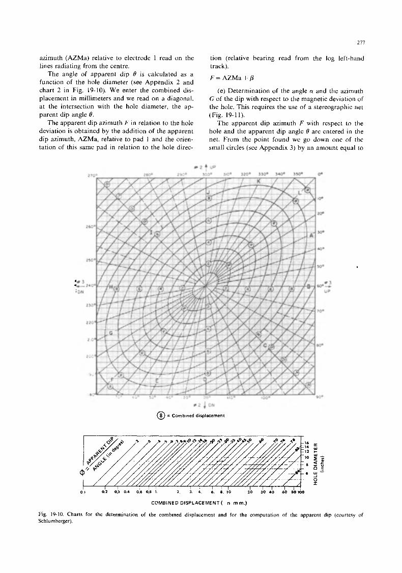
211
azimuth (AZMa) relative to electrode 1 read on the lines radiating from the centre.
The angle of apparent dip 8 is calculated as a function of the hole diameter (see Appendix 2 and chart 2 in Fig. 19-10). We enter the combined dis- placement in millimeters and we read on a diagonal, at the intersection with the hole diameter, the ap- parent dip angle 8.
The apparent dip azimuth F i n relation to the hole deviation is obtained by the addition of the apparent dip azimuth, AZMa, relative to pad 1 and the orien- tation of this same pad in relation to the hole direc-
tion (relative bearing read from the log left-hand track).
F = AZMa + /3 (e) Determination of the angle a and the azimuth
G of the dip with respect to the magnetic deviation of the hole. This requires the use of a stereographic net (Fig. 19-1 1).
The apparent dip azimuth F with respect to the hole and the apparent dip angle 8 are entered in the net. From the point found we go down one of the small circles (see Appendix 3) by an amount equal to
* 3
ON c
* 2 4 ON
@ = Combined displacement
16 14 12
10
8
6
0 1 0 1 0 , 3 0 4 0 6 0 . 8 1 1 3 4 6 8 . 1 0 20 30 4 0 60 80100
CCMBiNED DISPLACEMENT ( n m m.)
Fig. 19-10. Charts for the determination of the combined displacement and for the computation of the apparent dip (courtesy of Schlumberger).
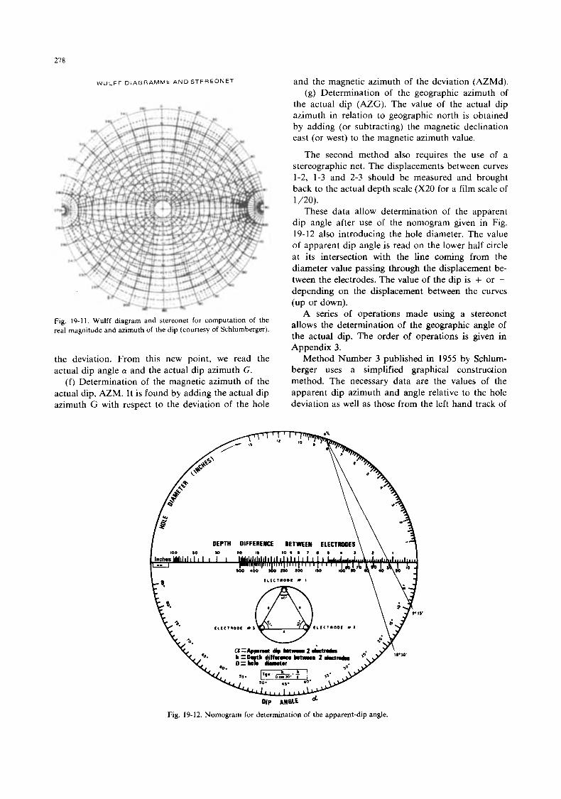
278
W U L F F D I A G R A M M E A N D STEREONE1
3% , O D .."
Fig. 19-1 1 . Wulff diagram and stereonet for computation of the real magnitude and azimuth of the dip (courtesy of Schlumberger).
the deviation. From this new point, we read the actual dip angle a! and the actual dip azimuth G.
(f) Determination of the magnetic azimuth of the actual dip, AZM. It is found by adding the actual dip azimuth G with respect to the deviation of the hole
and the magnetic azimuth of the deviation (AZMd). (g) Determination of the geographic azimuth of
the actual dip (AZG). The value of the actual dip azimuth in relation to geographic north is obtained by adding (or subtracting) the magnetic declination east (or west) to the magnetic azimuth value.
The second method also requires the use of a stereographic net. The displacements between curves 1-2, 1-3 and 2-3 should be measured and brought back to the actual depth scale (X20 for a film scale of
These data allow determination of the apparent dip angle after use of the nomogram given in Fig. 19-12 also introducing the hole diameter. The value of apparent dip angle is read on the lower half circle at its intersection with the line coming from the diameter value passing through the displacement be- tween the electrodes. The value of the dip is + or - depending on the displacement between the curves (up or down).
A series of operations made using a stereonet allows the determination of the geographic angle of the actual dip. The order of operations is given in Appendix 3.
Method Number 3 published in 1955 by Schlum- berger uses a simplified graphical construotion method. The necessary data are the values of the apparent dip azimuth and angle relative to the hole deviation as well as those from the left hand track of
1 /20).
DEPTH DIFFERENCE BETWEEN E l E C T m E S i o s m 7 s 4 s
Olp <WLE
Fig. 19-12. Nomogram for determination of the apparent-dip angle.
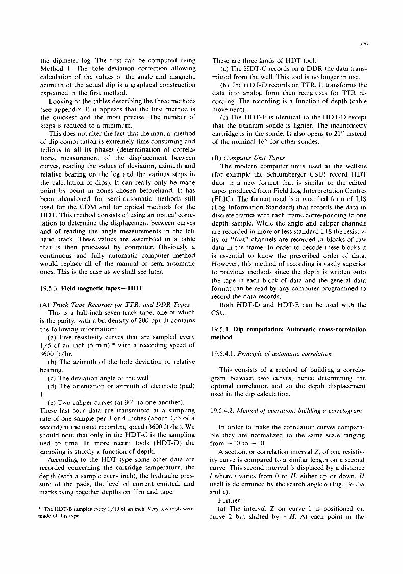
219
the dipmeter log. The first can be computed using Method 1. The hole deviation correction allowing calculation of the values of the angle and magnetic azimuth of the actual dip is a graphical construction explained in the first method.
Looking at the tables describing the three methods (see appendix 3) it appears that the first method is the quickest and the most precise. The number of steps is reduced to a minimum.
This does not alter the fact that the manual method of dip computation is extremely time consuming and tedious in all its phases (determination of correla- tions, measurement of the displacement between curves, reading the values of deviation, azimuth and relative bearing on the log and the various steps in the calculation of dips). It can really only be made point by point in zones chosen beforehand. It has been abandoned for semi-automatic methods still used for the CDM and for optical methods for the HDT. This method consists of using an optical corre- lation to determine the displacement between curves and of reading the angle measurements in the left hand track. These values are assembled in a table that is then processed by computer. Obviously a continuous and fully automatic computer method would replace all of the manual or semi-automatic ones. Thls is the case as we shall see later.
19.5.3. Field magnetic tapes-HDT
(A) Truck Tape Recorder (or TTR) and DDR Tapes This is a half-inch seven-track tape, one of which
is the parity, with a bit dqs i ty of 200 bpi. It contains the following information:
(a) Five resistivity curves that are sampled every 1/5 of an inch (5 mm) * with a recording speed of 3600 ft/hr.
(b) The azimuth of the hole deviation or relative bearing.
(c) The deviation angle of the well. (d) The orientation or azimuth of electrode (pad)
1. (e) Two caliper curves (at 90” to one another).
These last four data are transmitted at a sampling rate of one sample per 3 or 4 inches (about 1/3 of a second) at the usual recording speed (3600 ft/hr). We should note that only in the HDT-C is the sampling tied to time. In more recent tools (HDT-D) the sampling is strictly a function of depth.
According to the HDT type some other data are recorded concerning the cartridge temperature, the depth (with a sample every inch), the hydraulic pres- sure of the pads, the level of current emitted, and marks tying together depths on film and tape.
* The HDT-B samples every 1/10 of an inch. Very few tools were made of this type.
These are three kinds of HDT tool: (a) The HDT-C records on a DDR the data trans-
mitted from the well. This tool is no longer in use. (b) The HDT-D records on TTR. I t transforms the
data into analog form then redigitises for TTR re- cording. The recording is a function of depth (cable movement).
(c) The HDT-E is identical to the HDT-D except that the titanium sonde is lighter. The inclinometry cartridge is in the sonde. It also opens to 21” instead of the nominal 16” for other sondes.
(B) Computer Unit Tapes The modern computer units used at the wellsite
(for example the Schlumberger CSU) record HDT data in a new format that is similar to the edited tapes produced from Field Log Interpretation Centres (FLIC). The format used is a modified form of LIS (Log Information Standard) that records the data in discrete frames with each frame corresponding to one depth sample. While the angle and caliper channels are recorded in more or less standard LIS the resistiv- ity or “fast” channels are recorded in blocks of raw data in the frame. In order to decode these blocks it is essential to know the prescribed order of data. However, t h s method of recording is vastly superior to previous methods since the depth is written onto the tape in each block of data and the general data format can be read by any computer programmed to record the data records.
Both HDT-D and HDT-E can be used with the c s u .
19.5.4. Dip computation: Automatic cross-correlation method
19.5.4.1. Principle of automatic correlation
This consists of a method of building a correlo- gram between two curves, hence determining the optimal correlation and so the depth displacement used in the dip calculation.
19.5.4.2. Method of operation: building a correlogram
In order to make the correlation curves compara- ble they are normalized to the same scale ranging from - 10 to + 10.
A section, or correlation interval Z , of one resistiv- ity curve is compared to a similar length on a second curve. This second interval is displaced by a distance I where I varies from 0 to H , either up or down. H itself is determined by the search angle a (Fig. 19-13a and c).
Further: (a) The interval Z on curve 1 is positioned on
curve 2 but shifted by + H . At each point in the
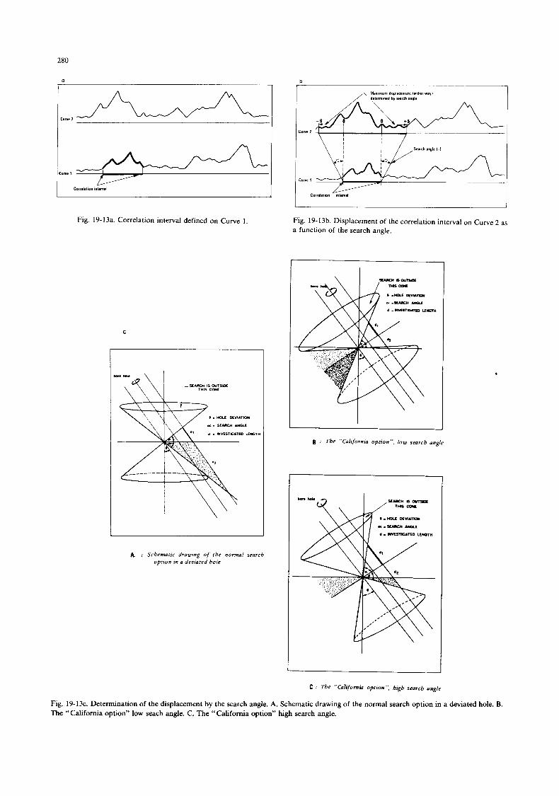
280
b
I !
Fig. 19-13a. Correlation interval defined on Curve 1
C
“.w \ I
A : Schematic drawing of the normal search option in a deuidted hole
Fig. 19-13b. Displacement of the correlation interval on Curve 2 as a function of the search angle.
B The “California opt ion”, low search ungle
c The “Catrfornua opt ion”, higb search angle
Fig. 19-13c. Determination of the displacement by the search angle. A. Schematic drawing of the normal search option in a deviated hole. B. The “California option” low seach angle. C. The “California option” high search angle.
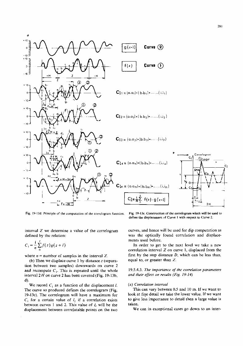
28 1
d
L n z
:-
c1, =(a.a,)+( b.b,)+ ........ ( i . i l )
c12= (o.02)+( b.b;l)+ ......... ( i . i l )
e
Fig. 19-13d. Principle of the computation of the correlogram function. Fig. 19-13e. Construction of the correlogram which will be used to define the displacement of Curve 1 with respect to Curve 2.
interval Z we determine a value of the correlogram defined by the relation:
where n = number of samples in the interval Z . (b) Then we displace curve 1 by distance z (separa-
tion between two samples) downwards on curve 2 and recompute C,. Ths is repeated until the whole interval 2 H on curve 2 has been covered (Fig. 19-13b,
We record C, as a function of the displacement 1. The curve so produced defines the correlogram (Fig. 19-13e). The correlogram will have a maximum for C, for a certain value of I , if a correlation exists between curves 1 and 2. This value of L will be the displacement between correlatable points on the two
4 .
curves, and hence will be used for dip computation as was the optically found correlation and displace- ments used before.
In order to get to the next level we take a new correlation interval Z on curve 1, displaced from the first by the step distance D, which can be less than, equal to, or greater than Z .
19.5.4.3. The importance of the correlation parameters and their effect on results (Fig. 19-1 4)
(a) Correlation interval This can vary between 0.5 and 10 m. If we want to
look at fiqe detail we take the lower value. If we want to give less importance to detail then a large value is taken.
We can in exceptional cases go down to an inter-
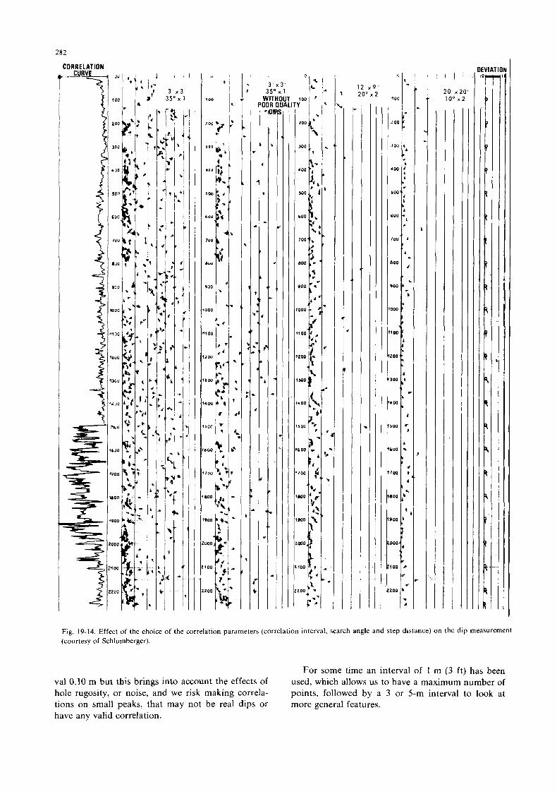
N" -.
I'
G I
LII
P
m
W M
m
- W
5
- 0 Fig. 19-14. Effect of the choice of the correlation parameters (correlation interval. search angle and step distance) on the dip measurement (courtesy of Schlurnberger).
For some time an interval of 1 m ( 3 ft) has been used, which allows us to have a maximum number of points, followed by a 3 or 5-m interval to look at more general features.
V a l 0.10 m but this brings into account the effects of hole rugosity, or noise, and we risk making cotrela- Lions on smaIl peaks, that may not be real dips or have any valid correlation.
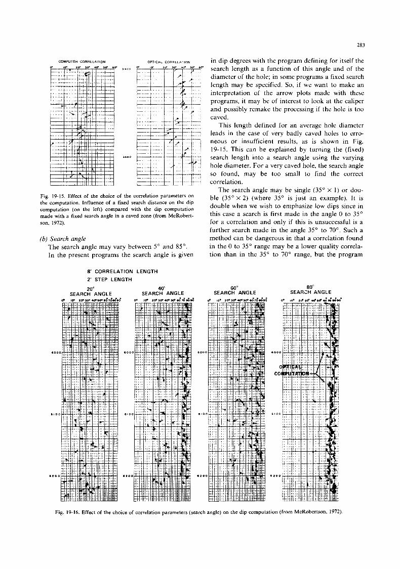
283
COMPUTER CORRELATION
3.00
,100
OPTICAL CORRELATION
0. 1 0 . Iff 30- .0- 50. 60.
I / / I P ' i
Fig. 19-15. Effect of the choice of the correlation parameters on the computation. Influence of a fixed search distance on the dip computation (on the left) compared with the dip computation made with a fixed search angle in a caved zone (from McRobert- son, 1972).
(b) Search angle The search angle may vary between 5" and 85". In the present programs the search angle is given
8 CORRELATION LENGTH
2' STEP LENGTH
20" SEARCH ANGLE
40" SEARCH ANGLE
80C
610
8 1 0
6 0 0
610
8 2 0
in dip degrees with the program defining for itself the search length as a function of this angle and of the diameter of the hole; in some programs a fixed search length may be specified. So, if we want to make an interpretation of the arrow plots made with these programs, it may be of interest to look at the caliper and possibly remake the processing if the hole is too caved.
This length defined for an average hole diameter leads in the case of very badly caved holes to erro- neous or insufficient results, as is shown in Fig. 19-15. This can be explained by turning the (fixed) search length into a search angle using the varying hole diameter. For a very caved hole, the search angle so found, may be too small to find the correct correlation.
The search angle may be single (35" x 1) or dou- ble (35" x 2 ) (where 35" is just an example). I t is double when we wish to emphasize low dips since in this case a search is first made in the angle 0 to 35" for a correlation and only if this is unsuccessful is a further search made in the angle 35" to 70". Such a method can be dangerous in that a correlation found in the 0 to 35" range may be a lower quality correla- tion than in the 35" to 70" range, but the program
. 60"
SEARCH ANGLE 80"
SEARCH ANGLE
Fig. 19-16. Effect of the choice of correlation parameters (search angle) on the dip computation (from McRobertson. 1972).
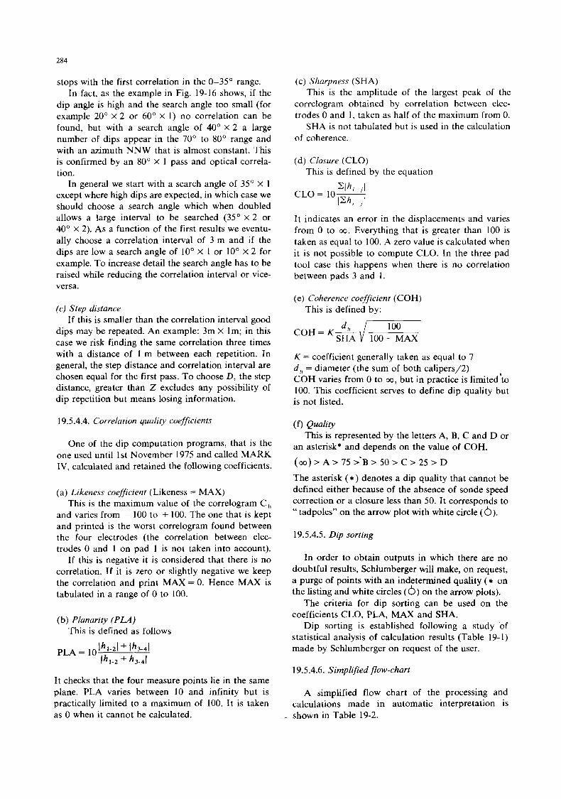
284
stops with the first correlation in the 0-35" range. In fact, as the example in Fig. 19-16 shows, if the
dip angle is high and the search angle too small (for example 20" x 2 or 60" X 1) no correlation can be found, but with a search angle of 40" X 2 a large number of dips appear in the 70" to 80" range and with an azimuth NNW that is almost constant. This is confirmed by an 80" X 1 pass and optical correla- tion.
In general we start with a search angle of 35" x 1 except where high dips are expected, in which case we should choose a search angle which when doubled allows a large interval to be searched (35" x 2 or 40" X 2). As a function of the first results we eventu- ally choose a correlation interval of 3 m and if the dips are low a search angle of 10" x 1 or 10" x 2 for example. To increase detail the search angle has to be raised while reducing the correlation interval or vice- versa.
(c) Step distance If this is smaller than the correlation interval good
dips may be repeated. An example: 3m X lm; in this case we risk finding the same correlation three times with a distance of 1 m between each repetition. In general, the step distance and correlation interval are chosen equal for the first pass. To choose D, the step distance, greater than Z excludes any possibility of dip repetition but means losing information.
19.5.4.4. Correlation quality coefficients
One of the dip computation programs, that is the one used until 1st November 1975 and called MARK IV, calculated and retained the following coefficients.
(a) Likeness coefficient (Likeness = MAX) This is the maximum value of the correlogram C,
and varies from - 100 to + 100. The one that is kept and printed is the worst correlogram found between the four electrodes (the correlation between elec- trodes 0 and 1 on pad 1 is not taken into account).
If this is negative it is considered that there is no correlation. If it is zero or slightly negative we keep the correlation and print MAX = 0. Hence MAX is tabulated in a range of 0 to 100.
(b) Planarity (PLA) This is defined as follows
It checks that the four measure points lie in the same plane. PLA varies between 10 and infinity but is practically limited to a maximum of 100. It is taken as 0 when it cannot be calculated.
(c) Sharpness (SHA) This is the amplitude of the largest peak of the
correlogram obtained by correlation between elec- trodes 0 and 1, taken as half of the maximum from 0.
SHA is not tabulated but is used in the calculation of coherence.
(d) Closure (CLO) This is defined by the equation
It indicates an error in the displacements and varies from 0 to co. Everything that is greater than 100 is taken as equal to 100. A zero value is calculated when it is not possible to compute CLO. In the three pad tool case this happens when there is no correlation between pads 3 and 1.
(e) Coherence coefficient (COH) This is defined by:
100 COH = K - SHA d h J 100-MAX
K = coefficient generally taken as equal to 7 d, = diameter (the sum of both calipers/2) COH varies from 0 to co, but in practice is limited'to 100. This coefficient serves to define dip quality but is not listed.
( f ) Quality
an asterisk* and depends on the value of COH.
(co) > A > 75 >'B > 50 > C > 25 > D The asterisk ( * ) denotes a dip quality that cannot be defined either because of the absence of sonde speed correction or a closure less than 50. It corresponds to "tadpoles" on the arrow plot with white circle (6).
This is represented by the letters A, B, C and D or
19.5.4.5. Dip sorting
In order to obtain outputs in which there are no doubtful results, Schlumberger will make, on request, a purge of points with an indetermined quality ( * on the listing and white circles (6) on the arrow plots).
The criteria for dip sorting can be used on the coefficients CLO, PLA, MAX and SHA.
Dip sorting is established following a study 'of statistical analysis of calculation results (Table 19- 1) made by Schlumberger on request of the user.
19.5.4.6. Simplified flow-chart
A simplified flow chart of the processing and calculations made in automatic interpretation is
- shown in Table 19-2.
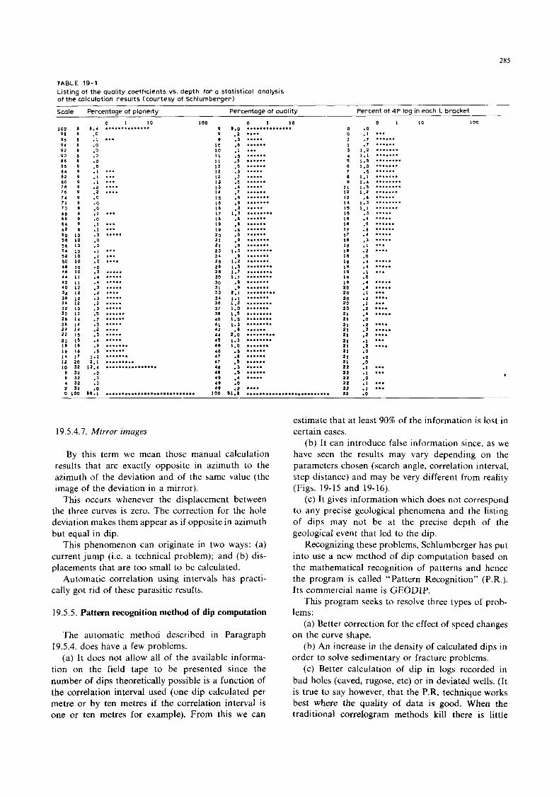
285
TABLE 19-1 Listing of the quality coefficients vs. depth for a statistical analysis of the calculation results (courtesy of Schlurnberger)
-
- Scale Percentage of planeity Percentage of quality Percent of 4 P log in each L bracket
100 96 9 6 94 92 90 88 6 ) 8 4 82 8 0 7 8 76 7 4 72 70 68 6 6 6 4 b 2 b o 56 56 5 4
50 4 8 4 6 4 4
4 2 40 3 8 36 34 32 30 28 26 a4 1 2
1 8 I 6 1 4 I2 10
8 b 4 2
5 a
a o
8 8 8 8 8 8 8 8 9 9 V 9 9 9 9 0 P 0 9 9
LO LO 1 0 LO LO 10 I0 I0 1 1 I 1 12 I2 12 1 2 I 3 I 3 I4 1 4 1 4 1, I 5 I 6 I 8 1 7 20
32 32 32
12 3 2
8.4 .o . I .o .O .o .o .Q . l . I . I . z . z .o .o .o . I .O . I . I . 3 .o .o . I . I . 2 .O .J .4 . 4
.s
. z
. J
. 3
..I
.5
.7
. 3
.I
.s
.4
.9
.I 1.2 2.1
1 2 . 4 .O .o .O .n
0 1 LO .............. ...
... ... ... .... ....
... ... ... .....
... ... ....
..... ..... ..... ..... .... ..... ..... ..... ...... ...... ..... .... ..... ..... ....... ...... ....... ......... ................
100 9 9 V
LO 10 I 1 I 1 I2 I2 12 I 3 I 3 I4 I5 I 6 I 6 I7 18 I9 I9 20 2 1 21 23 2 4 25 2 b 28 SO 30 31 3 3 s4 ss 3 7 38 4 0 4 1 42 4 4 4, 4b 4b 47 I7 48 48 4 V 4 0 40
0 1 LO ................. ...... ....... ........ ..... ........ ........ ........ ....... ....... ........ ....... ........ ......... ......... - 3 .....
1 . 3 ........ ........ ........ ........ ........ ......... ......... 1 . 3 ........ ......... 1.2 ....... ........... 1.7 ........ 1.7 ........ ......... ......... ............ 1.1 ....... 1.0 ....... I . , ........ I . , ........ 1.3 ........
0 0 I I 3 4 I 8 7 8 9
1 1 I2 12 14 15 I , I 6 1 1 I7
I 8 18 I 8 I 8 18 19 I P I 0 19 20 20 20 20 20 21 2 1
17
1 . 3 ........ - 8 ......
2.0 ......... 1.3 ........ 1.0 ....... ., ......
- 6 ...... - 3 ...... - 3 ..... ., ...... ....... - 0 _ - ...... 22 ~-
6 l o o r 8 ; i ............................ LOO a i i i ............................
0 1 I0
19.5.4.1. Mirror images
By this term we mean those manual calculation results that are exactly opposite in azimuth to the azimuth of the deviation and of the same value (the image of the deviation in a mirror).
This occurs whenever the displacement between the three curves is zero. The correction for the hole deviation makes them appear as if opposite in azimuth but equal in dip.
This phenomenon can originate in two ways: (a) current jump (i.e. a technical problem); and (b) dis- placements that are too small to be calculated.
Automatic correlation using intervals has practi- cally got rid of these parasitic results.
19.5.5. Pattern recognition method of dip computation
The automatic method described in Paragraph 19.5.4. does have a few problems.
(a) It does not allow all of the available informa- tion on the field tape to be presented since the number of dips theoretically possible is a function of the correlation interval used (one dip calculated per metre or by ten metres if the correlation interval is one or ten metres for example). From this we can
estimate that at least 90% of the information is lost in certain cases.
(b) I t can introduce false information since, as we have seen the results may vary depending on the parameters chosen (search angle, correlation interval, step distance) and may be very different from reality (Figs. 19-15 and 19-16).
(c) I t gives information which does not correspond to any precise geological phenomena and the listing of dips may not be at the precise depth of the geological event that led to the dip.
Recognizing these problems, Schlumberger has put into use a new method of dip computation based on the mathematical recognition of patterns and hence the program is called “Pattern Recognition” (P.R.). Its commercial name is GEODIP.
This program seeks to resolve three types of prob- lems:
(a) Better correction for the effect of speed changes on the curve shape.
(b) An increase in the density of calculated dips in order to solve sedimentary or fracture problems.
(c) Better calculation of dip in logs recorded in bad holes (caved, rugose, etc) or in deviated wells. (It is true to say however, that the P.R. technique works best where the quality of data is good. When the traditional correlogram methods lull there is little
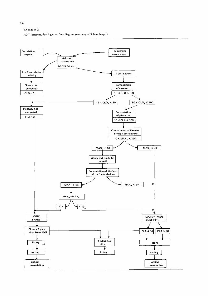
286
Correlation interval
TABLE 19-2
HDT interpretation logic - flow diagram (courtesy of Schlumberger)
Maximum search angle
( O o r 1 0 t o 1 0 0 ) P L A < 5 0
correlations
1-2.2-3.3-4.4-1
1 or 2 correlations missing
4 correlations
I
P L A > W
Closure not computed
I CLO=O I
Planarity not el I P L A = J
Computation of closure
I lo<cLo4 loo1 e 10 4 CLO, < 50 50 4 CLO, 4 100 b Computation of planarity
Computation of likeness I of the 4 correlations
0 4 MAX, 4 100
MAX, < 70 MAX, > 70
1
1 Which pad would be
unused ?
Computation of likeness of the 3 correlations . d MAX, > 50 * MAX, < 50
4 MAX, -MAX,
1 10 < < 10 I I
LOGIC 3 PADS
LOGIC4 PADS BEST FIT ~
b sorting h listing sorting
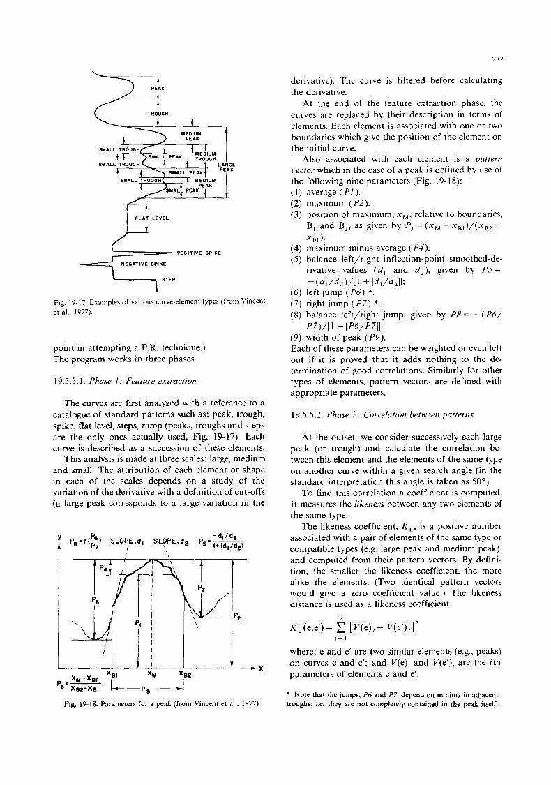
287
f i TROUGH
POSIT IVE SPIKE -+TIp NEGATIVE SPIKE
Fig. 19-17. Examples of various curve-element types (from Vincent et al.. 1977).
point in attempting a P.R. technique.) The program works in three phases.
1 9.5.5.1. Phase I : Feature extraction
The curves are first analyzed with a reference to a catalogue of standard patterns such as: peak, trough, spike, flat level, steps, ramp (peaks, troughs and steps are the only ones actually used, Fig. 19-17). Each curve is described as a succession of these elements.
This analysis is made at three scales: large, medium and small. The attribution of each element or shape in each of the scales depends on a study of the variation of the derivative with a definition of cut-offs (a large peak corresponds to a large variation in the
Fig. 19-18. Parameters for a peak (from Vincent et al., 1977).
derivative). The curve is filtered before calculating the derivative.
At the end of the feature extraction phase, the curves are replaced by their description in terms of elements. Each element is associated with one or two boundaries which give the position of the element on the initial curve.
Also associated with each element is a pattern vector which in the case of a peak is defined by use of the following nine parameters (Fig. 19-1 8): (1) average ( P I ). ( 2 ) maximum ( P 2 ) . (3) position of maximum, x,, relative to boundaries,
B, and B,, as given by P3 = ( x , - xsl)/(xH, - XI31 ).
(4) maximum minus average ( P 4 ) . ( 5 ) balance left/right inflection-point smoothed-de-
rivative values ( d , and d,), given by P5 =
-(d,/d2)/[1 + ld,/d2ll; (6) left jump ( P 6 ) *. (7) right jump ( P 7 ) *. (8) balance left/right jump, given by P8 = -( P6/
P 7 ) / [ 1 + IP6/P71]. (9) width of peak ( P 9 ) . Each of these parameters can be weighted or even left out if it is proved that it adds nothing to the de- termination of good correlations. Similarly for other types of elements, pattern vectors are defined with appropriate parameters.
19.5.5.2. Phase 2: Correlation between patterns
At the outset, we consider successively each large peak (or trough) and calculate the correlation be- tween this element and the elements of the same type on another curve within a given search angle (in the standard interpretation this angle is taken as SO0).
To find this correlation a coefficient is computed. It measures the likeness between any two elements of the same type.
The likeness coefficient, K,, is a positive number associated with a pair of elements of the same type or compatible types (e.g. large peak and medium peak), and computed from their pattern vectors. By defini- tion, the smaller the likeness coefficient, the more alike the elements. (Two identical pattern vectors would give a zero coefficient value.) The likeness distance is used as a likeness coefficient
9
K , (e,e’) = C [ v(e) , - ~ e ’ ) , I 2
where: e and e’ are two similar elements (e.g., peaks) on curves c and c’; and V(e), and V(e’), are the ith parameters of elements e and e’.
r = l
* Note that the jumps, P6 and P7, depend on minima in adjacent troughs; i.e. they are not completely contained in the peak itself.
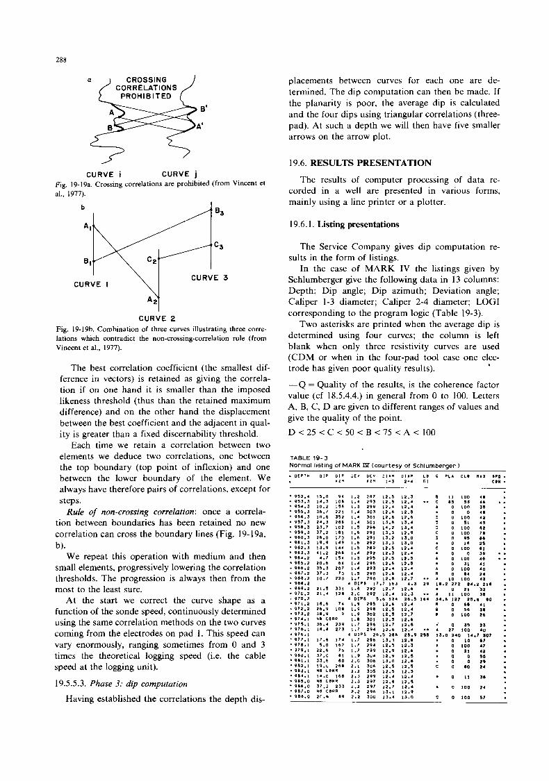
288
placements between curves for each one are de- termined. The dip computation can then be made. If the planarity is poor, the average dip is calculated and the four dips using triangular correlations (three- pad). At such a depth we will then have five smaller arrows on the arrow plot.
CURVE i CURVE j Fig. 19-19a. Crossing correlations are prohibited (from Vincent et al., 1977).
b
A l '
B l
CURVE 3 CURVE I
CURVE 2 Fig. 19-19b. Combination of three curves illustrating three corre- lations which contradict the non-crossing-correlation rule (from Vincent et al., 1977).
The best correlation coefficient (the smallest dif- ference in vectors) is retained as giving the correla- tion if on one hand it is smaller than the imposed likeness threshold (thus than the retained maximum difference) and on the other hand the displacement between the best coefficient and the adjacent in qual- ity is greater than a fixed discernability threshold.
Each time we retain a correlation between two elements we deduce two correlations, one between the top boundary (top point of inflexion) and one between the lower boundary of the element. We always have therefore pairs of correlations, except for steps.
Rule of non-crossing correlation: once a correla- tion between boundaries has been retained no new correlation can cross the boundary lines (Fig. 19-19a, b).
We repeat this operation with medium and then small elements, progressively lowering the correlation thresholds. The progression is always then from the most to the least sure.
At the start we correct the curve shape as a function of the sonde speed, continuously determined using the same correlation methods on the two curves coming from the electrodes on pad 1. This speed can vary enormously, ranging sometimes from 0 and 3 times the theoretical logging speed (i.e. the cable speed at the logging unit).
19.5.5.3. Phase 3: dip computation
Having established the correlations the depth dis-
19.6. RESULTS PRESENTATION
The results of computer processing of data re- corded in a well are presented in various forms, mainly using a line printer or a plotter.
19.6.1. Listing presentations
The Service Company gives dip computation re- sults in the form of listings.
In the case of MARK IV the listings given by Schlumberger give the following data in 13 columns: Depth; Dip angle; Dip azimuth; Deviation angle; Caliper 1-3 diameter; Caliper 2-4 diameter; LOG1 corresponding to the program logic (Table 19-3).
Two asterisks are printed when the average dip is determined using four curves; the column is left blank when only three resistivity curves are used (CDM or when in the four-pad tool case one elec- trode has given poor quality results).
-Q = Quality of the results, is the coherence factor value (cf 18.5.4.4.) in general from 0 to 100. Letters A, B, C , D are given to different ranges of values and give the quality of the point. D < 25 < C < 50 < B < 75 < A < 100
.
TABLE 19-3 Normal listinq of MARK JI (courtesv of Schlurnberaer)
. D E P T H DIP DIP U E V D E V D I A M 0 1 4 M L U 0 PLA C L 1 M I X 8 P D . 1 1 " 1111 1 - 3 2.4 GI con -
952.1 953.3 - 95a.3
* 955.3 . 956.3 . 957.3 . 958.3 * 959.3 - 960.3 . 961.3 962.3
* 963.3 * 964.2 * 965.2 * 966.2 - 967.2 - 968.2 * 961.2 - 969.2 - 97U.2 - 970.7 a 971.2 * 972.2 .973.2 * 974.1 -975.1 . 97b.l * 97b.I 977.1
. 279.1 - 98U.l 901. I . 982.1
* 98J.L .984.I - 985.0 - 986.0 . 917.0 . 98L1.0
* 978.1
* ~ - C O R R 36.4 239 18.8 273
17.6 I74 5.0 1 6 2
22.6 73 37.0 61 33.b 80 19.U 268 NO L O R R 14.0 168 NO L 8 Y R 37.2 233 NO CORR 20.6 89
1 5 . 0 9L 14.3 1 0 8 10.2 I58 36.7 221 10.6 352 24.3 288 23.7 I02 37.2 1 8 1 26.0 I70 19.9 I49 13.9 I44 4 1 . 2 268 4.7 I54
20.6 6 4 3>.3 207 37.3 70 10.7 220
21.5 331 2 1 . 4 128
1.2 287 1 2 . 5 1.4 295 12.5 1.3 299 12.. 1.4 303 12.6 1 . 4 3 0 1 12.6 1 . 4 3 0 1 1 3 . 6 1.5 296 1 4 . 2 1.6 291 13.3 1.6 291 13.2 1 . 6 292 13.3 1.5 289 12.5 1 . 4 292 12.3 1.3 295 12.5 1.4 296 12.6 1 . 4 293 12.4 1.5 290 12.6 1.7 290 12.6
4 D I P S 17.7 163 1.8 292 12.7 2.0 292 12.4
4 DIPS 5.0 1 3 4 18.6 74 1.9 295 12.6 26.9 I08 1.0 298 12.5 38.9 9 1.9 302 12.5
1.8 301 12.5 1.7 296 12.7 1.7 294 12.6
4 U l P S 26.5 286 1.7 296 13.1 1.7 294 12.5 1 .7 299 12.9 1.9 3u4 12.9 2.0 306 13 .0 2.1 300 12.5 2.2 305 12.5 2.3 299 1 2 . 4 2.3 297 12.8 2.2 297 12.7 2.2 296 13.1 2.2 300 13.4
12.3 12.4 .. 1 2 . 4 12.5 12.6 13.4 13.4 12.9
13.0 1 2 . 4 12.4 12.5 12.5 12.4 12.4 12.7 ..
4.3 29 12.6
13.0
12.3 .. 1 2 . 4 12.4 12.7 12.6 12.6 12.4 * * 25.9 255
12.1 12.3 12.6 12.5 12.6 12.5 12.3 12.4 12.5 12.4 12.9 13.0
26.5 I64
8 I 1 100 4I C 85 53 4 6 I 0 LOO 35 . 0 0 4 8 D u 100 4 1 D 0 SI 45 0 0 100 82 C 0 100 7 1 D 0 05 16
0 I 6 25
0 0 3 0 1 0 100 4 6
0 31 4 1 1 0 100 4 0 0 0 I 4 24 I 1 0 100 4 s 11.2 272 24.2 211
0 21 YA A I 1 I U O 38 34.6 127 25.U @ O 0 0 66 4 1 B 0 56 38 D 0 LOO 21
c 0 100 11
i 0 35 23 A 27 LOO 40 13.0 140 14.7 a07 * 0 I D b7 4 0 100 47
o 11 42 0 0 5 0 . 0 0 2 9
C 0 60 24
0 1 1 36
A 0 LOO 24
c 0 LOO 57
..
.. ..
-
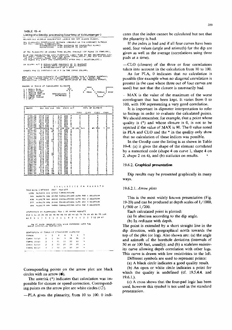
289
TABLE 19-4 Listing of a Geodip processing (courtesy of Schlumberger 1 __- B u u ~ D b P l t S r F T d F L n S L U 1 # t h T A Y Y L A X E Y S A Y t hOT AL-bKS P L I N A W .
T Y L P L A N A N l l X C O C Y F I C I L N T UCYFNDS L I N L A R L Y UN THE D I S T A N C E LLTmELN THF ThlJ L'IAG11NhL CORRELATIONS.
P L A N A R I T Y = I U U WhLh D I S T A N C E .O I P L Y F E C T L Y P L A N t l P L b N b R I T Y r O * H E * D I S T I N C F 15 I h C H E S
I F ThL P L A N A h l I Y 15 H l G H C I l T H h N 8 0 , T Y L AVCMACE U I P P L A N L IS CONPUTEU.
1 Y CULUHV n / T b MLAY5'LIJ.EP bUU*UAYX UF A N E L L R L N T T mEAbdS~UPPEP h O U N 0 h R Y OF Ah E L L L F l l T S *tbNS:BUUNDbSI OF A STLP
U M U S F U PAU 15 I N D I C A I L D 1 ( X A 0 I N T H E CURVE COLUMN.
.... ..I... COOING l l t T Y P t S UF CDRYELAlLD L L L * E N T $
5 I A 1 1 S T I C S O h U E S U L T S
T H I S . Z I I N t C U N T A I N S 2 5 3 1 MEDLIL IS
1 2 0 9 H t S U L l S AhL I - P A V C I I R H L L A I I U h S
3UY "LSULTS I R E 3 -YAU C U Y H L L A T I U I S .1Tn PAD I D E L O T I I I N
4 3 8 MLDI ILTS A Y L J - P I D C U R R L L A T I O h S W I T H P A 0 2 U E L E T I U N
2 1 1 HLSULTS A Y E 3-PAD C O H ~ L L A T l V l b W I T H P b U J U E L E T l U l l
3 0 4 h L D U L 1 S 111) ) - P A 0 C U Y I ( L L I T I 0 I S 1 1 1 H PAU 4 V L L L T I O N
S T A T I S I I C S U* Y L h 1 I A h I T Y I PLA ) V V 4-PAU RESULTS
P I 0 5 I u 15 2 u 15 3" 35 4 u 4 5 hU 3 5 b U b s l u 1 5 M u U S 90 91, 1uO
s i o 0 u u 0 0 u 0 " 1 0 0 u 1 1 2 l l 2 I U P l
Corresponding points on the arrow plot are black circles with an arrow (d).
The asterisk (*) indicates that calculation was im- possible for closure or speed correction. Correspond- ing points on the arrow plot are white circles (6). -PLA gives the planarity, from 10 to 100. 0 indi-
cates that the index cannot be calculated but not that the planarity is bad.
If the index is bad and if all four curves have been used, four values (angle and azimuth) for the dip are given as well as the average (correlations using three pads at a time).
-CLO (closure) of the three or four correlations taken into account in the calculation from 10 to 100.
As for PLA, 0 indicates that no calculation is possible (for example when no diagonal correlation is present in the case where three out of four curves are used) but not that the closure is necessarily bad.
-MAX is the value of the maximum of the worst correlogram that has been kept. It varies from 0 to 100, with 100 representing a very good correlation.
It is important in dipmeter interpretation to refer to listings in order to evaluate the calculated points. We should remember, for example, that a point whose quality is (*) and whose closure is 0, is not to be rejected if the value of MAX is 90. The 0 value noted in PLA and CLO and the * in the quality only show that no calculation of these indices was possible.
In the Geodip case the listing is as shown in Table 19-4: (a) it gives the shape of the element correlated by a numerical code (shape 4 on curve 1, shape 4 on 2, shape 2 on 4), and (b) statistics on results. '
19.6.2. Graphical presentation
Dip results may be presented graphically in many ways.
19.6.2.1. Arrow plots
T h s is the most widely known presentation (Fig. 19-20) and can be produced at depth scales of 1/1000, 1/500 or 1/200.
Each calculated point is plotted: (a) In abscissa according to the dip angle. (b) In ordinate with depth.
The point is extended by a short straight line in the dip direction, with geographical north towards the top of the plot (or log). Also shown are: (a) the angle and azimuth of the borehole deviation (intervals of 50 m or 100 feet, usually); and (b) a scaleless resistiv- ity curve allowing depth correlation with other logs. This curve is drawn with low resistivities to the left.
Different symbols are used to represent points: (a) A black circle indicates a good quality result. (b) An open or white circle indicates a point for
which the quality is undefined (cf. 19.5.4.4. and 19.6.1.).
(c) A cross shows that the four-pad logic has been used, however this symbol is not used in the standard presentation.
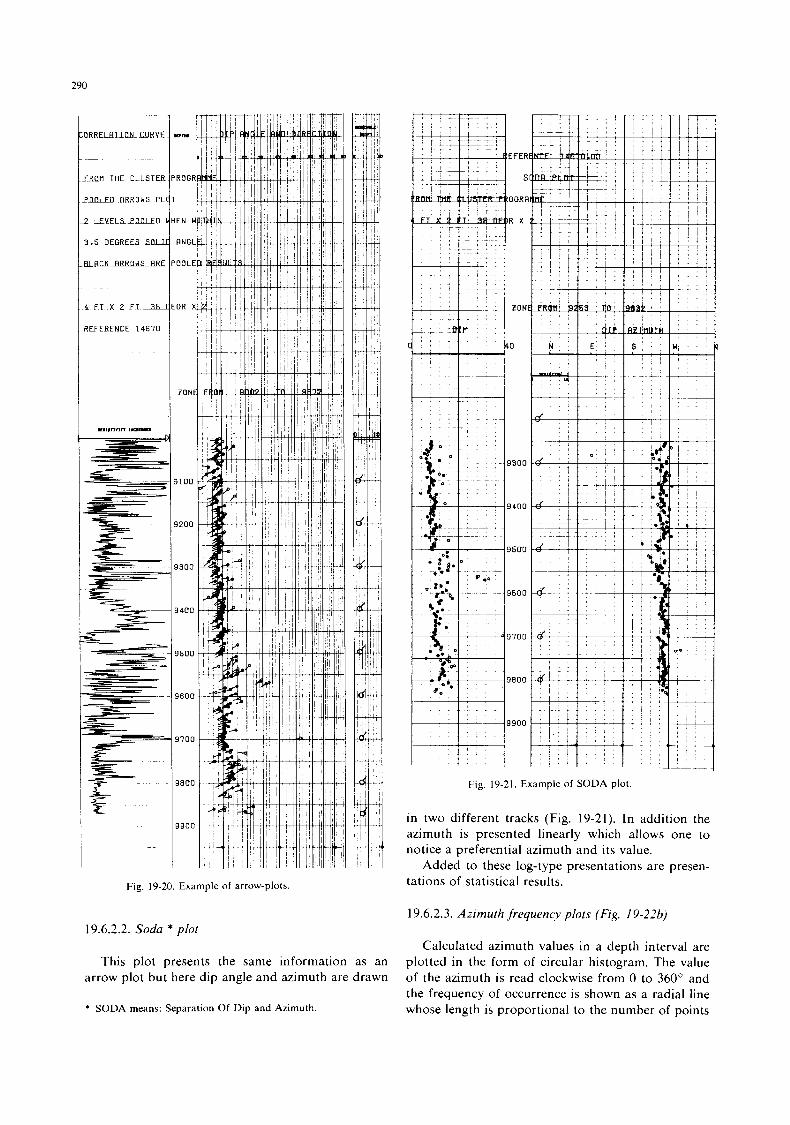
290
lL.w
ROO
EN
ANG
OOL
OR
ZOE
310(
3201
3301
3401
3501
960
970
980
990
Fig. 19-20. Example of arrow-plots.
EFER
s
OGRF
R X
ZON
0
f 1
9300
9400
9500
9600
9700
9800
I
t I
--+-
Fig. 19-21. Example of SODA plot.
in two different tracks (Fig. 19-21). In addition the azimuth is presented linearly which allows one to notice a preferential azimuth and its value.
Added to these log-type presentations are presen- tations of statistical results.
19.6.2.3. Azimuth frequency plots (Fig. 19-226) 19.6.2.2. Soda * plot
This plot presents the same information as an arrow plot but here dip angle and azimuth are drawn
Calculated azimuth values in a depth interval are plotted in the form of circular histogram. The value of the azimuth is read clockwise from 0 to 360" and the frequency of occurrence is shown as a radial line whose length is proportional to the number of points
I
* SODA means: Separation Of Dip and Azimuth.
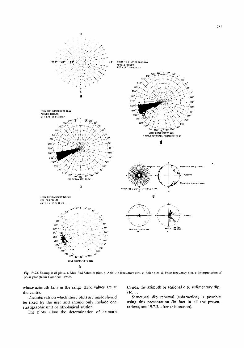
29 1
N
- E FROM THE CLUSTER PROGRAM POOLED RESULTS 4 FT X 2 F T 3 5 OEGR X 2
S
a
FROM THE CLUSTER PROGRAM POOLEO RESULTS 4 FT X : 2 F T 3 5 OEGR X 2
ZONE FROM 9253 TO 9832
b
FROM THE CLUSTER P R O G R A M POOLED RESULTS 4 FT X z F T A 5 DEAR X-2- --
340a3500 0- 10" z0' 30'
40 . ~ 50'
330" 320- , .
310°,' . _.
ZONE FROM 9253 TO 9832 FREOUENCY SCALE FROM CENTER 60
d
M O D I F I E D S C H h l D T D I A G R A M ,./ ,<I
e 0 .. . E W Y E Channel
.. . . .. I
POLAR D I A G R A M "OI.EE 0 01"s 1,) I
210" 150- 2*"190-1800 1 70"1WD
ZONE FROM 9253 TO 9832
C
Fig. 19-22. Examples of plots. a. Modified Schmidt plot. b. Azimuth frequency plot. c. Polar plot. d. Polar frequency plot. e. Interpretation of polar plot (from Campbell. 1969).
whose azimuth falls in the range. Zero values are at the centre. etc.. . .
The intervals on which those plots are made should be fixed by the user and should only include one stratigraphic unit or lithological section.
The plots allow the determination of azimuth
trends, the azimuth or regional dip, sedimentary dip,
Structural dip removal (subtraction) is possible using this presentation (in fact in all the presen- tations, see 19.7.3. after this section).
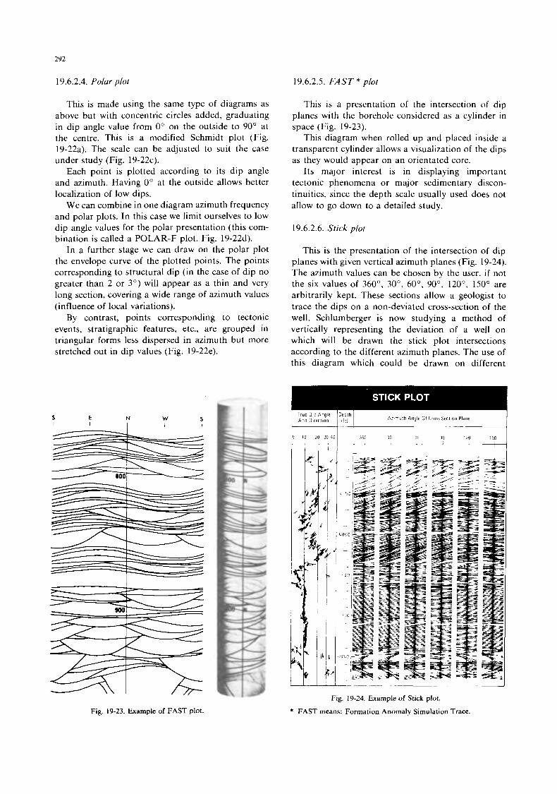
292
19.6.2.4. Polar plot 19.6.2.5. FAST * plot
This is made using the same type of diagrams as above but with concentric circles added, graduating in dip angle value from 0" on the outside to 90" at the centre. This is a modified Schmidt plot (Fig. 19-22a). The scale can be adjusted to suit the case under study (Fig. 19-22c).
Each point is plotted according to its dip angle and azimuth. Having 0" at the outside allows better localization of low dips.
We can combine in one diagram azimuth frequency and polar plots. In this case we limit ourselves to low dip angle values for the polar presentation (this com- bination is called a POLAR-F plot, Fig. 19-22d).
In a further stage we can draw on the polar plot the envelope curve of the plotted points. The points corresponding to structural dip (in the case of dip no greater than 2 or 3") will appear as a thin and very long section, covering a wide range of azimuth values (influence of local variations).
By contrast, points corresponding to tectonic events, stratigraphic features, etc., are grouped in triangular forms less dispersed in azimuth but more stretched out in dip values (Fig. 19-22e).
S E N W S I I I I I
This is a presentation of the intersection of dip planes with the borehole considered as a cylinder in space (Fig. 19-23).
This diagram when rolled up and placed inside a transparent cylinder allows a visualization of the dips as they would appear on an orientated core.
Its major interest is in displaying important tectonic phenomena or major sedimentary discon- tinuities, since the depth scale usually used does not allow to go down to a detailed study.
19.6.2.6. Stick plot
This is the presentation of the intersection of dip planes with given vertical azimuth planes (Fig. 19-24). The azimuth values can be chosen by the user, i f not the six values of 360", 30", 60". 90", 120", 150" are arbitrarily kept. These sections allow a geologist to trace the dips on a non-deviated cross-section of the well. Schlumberger is now studying a method of vertically representing the deviation of a well on which will be drawn the stick plot intersections according to the different azimuth planes. The use of this diagram which could be drawn on different *
True O i p Angle And Direc t ion
I 10 20 30 41
i Azimuth Angle 01 Cross Section Plane -
Fig. 19-24. Example of Stick plot.
* FAST means: Formation Anomaly Simulation Trace. Fig. 19-23. Example of FAST plot.
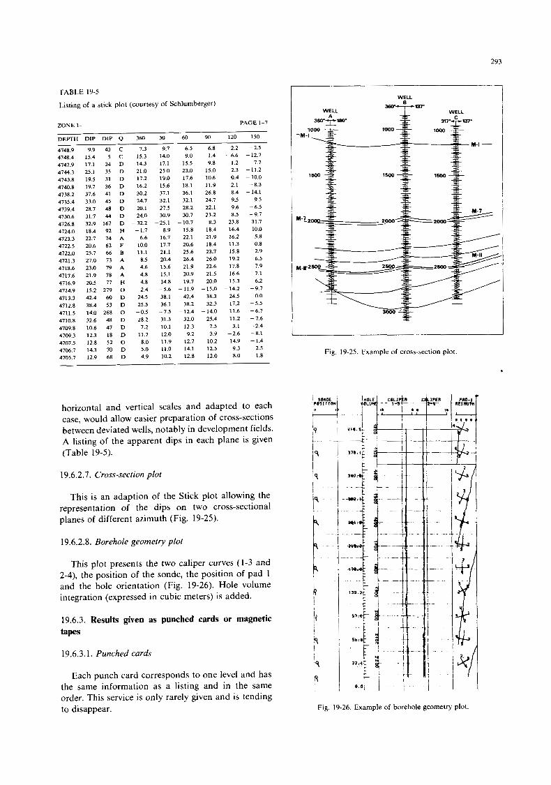
293
TABLE 19-5
Listing of a stick plot (courtesy of Schlumberger)
ZONE 1- PAGE 1-7
~
DEPTH DIP DIP Q 360 30 60
4748.9 9.9 43 C 7.3 9.7 6.5
4748.4 15.4 5 C 15.3 14.0 9.0
4747.9 17.1 34 D 14.3 17.1 15.5
4744.3 25 1 35 D 21.0 25.0 23.0
4743.8 19.5 31 D 17.2 19.0 17.6
4740.8 19.7 36 D 16.2 15.6 18.1
4738.2 37.6 41 D 30.2 37.1 36.1
4735.4 33.0 45 D 24.7 32.1 32.1
4739.4 28.7 48 D 20.1 27.5 28.2
4730.6 31.7 44 D 24.0 30.9 30.7
4726.8 32.9 167 D -32.2 -25.1 -10.7
4724.0 18.4 92 H -1.7 8.9 15.8
4723.3 22.7 74 A 6.6 16.7 22.1
4722.5 20.6 62 F 10.0 17.7 20.6
4722.0 25.7 66 B 11.1 21.1 25.6
4721.3 27.0 73 A 8.5 20.4 26.4
4717.6 21.9 78 A 4.8 15.1 20.9
4716.9 20.5 77 H 4.8 14.8 19.7
4714.9 15.2 279 0 2.4 -5.6 -11.9
4713.3 42.4 60 D 24.5 38.1 42.4
4712.8 38.4 53 D 25.5 36.1 38.2
4711.5 14.0 268 0 -0.5 -7.5 -12.4
4710.8 32.6 48 D 28.2 31.3 32.0
4709.8 10.6 47 D 7.2 10.1 12.3
4709.3 12.3 18 D 11.7 12.0 9.2
4707.5 12.8 52 0 8.0 11.9 12.7
4706.7 14.3 70 D 5.0 11.0 14.1
4705.7 12.9 68 D 4.9 10.2 12.8
4718.6 23.0 79 A 4.6 15.6 21.9
90 120 150
6.8 1.4 9.8 15.0 10.6 11.9 26.8 24.7 22.1 23.2 8.3 18.4 21.9 18.4 23.7 26.0 22.6 21.5 20.0
- 15.0 38.3 32.3
- 14.0 25.4 7.5 3.9 10.2 12.5 12.0
2.2 - 6.6 1.2 2.3 0.4 2.1 8.4 9.5 9.6 8.5 23.8 16.4 16.2 11.3 15.8 19.2 17.8 16.6 15.3
- 14.2 24.5 17.2 11.6 11.2 3.1
- 2.6 14.9 9.3 8.0
- 2.5 - 12.7 - 7.7 -11.2 - 10.0 - 8.3 - 14.1 - 9.5 -6.5 - 9.7 31.7 10.0 5.8 0.8 2.9 6.5 7.9 7.1 6.2
-9.7 0.0
- 5.5 -6.7 - 7.6 - 2.4 - 8.1 - 1.4 2.5 1.8
horizontal and vertical scales and adapted to each case, would allow easier preparation of cross-sections between deviated wells, notably in development fields. A listing of the apparent dips in each plane is given (Table 19-5).
19.6.2.7. Cross-section plot
This is an adaption of the Stick plot allowing the representation of the dips on two cross-sectional planes of different azimuth (Fig. 19-25).
19.6.2.8. Borehole geometry plot
This plot presents the two caliper curves (1-3 and 2-4), the position of the sonde, the position of pad 1 and the hole orientation (Fig. 19-26). Hole volume integration (expressed in cubic meters) is added.
19.6.3. Results given as punched cards or magnetic tapes
19.6.3.1. Punched cards
Each punch card corresponds to one level and has the same information as a listing and in the same order. This service is only rarely given and is tending to disappear.
WELL
~~~ ~ -
Fig. 19-25. Example of cross-section plot.
.
Fig. 19-26. Example of borehole geometry plot.
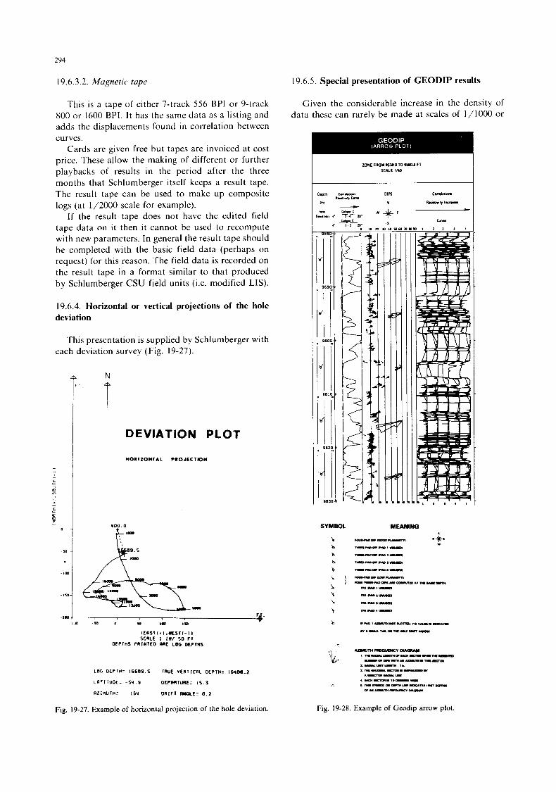
294
19.6.3.2. Magnetic. tape 19.6.5. Special presentation of CEODIP results
This is a tape of either 7-track 556 BPI or 9-track 800 or 1600 BPI. I t has the same data as a listing and adds the displacements found in correlation between curves.
Cards are given free but tapes are invoiced at cost price. These allow the making of different or further playbacks of results in the period after the three months that Schlumberger itself keeps a result tape. The result tape can be used to make up composite logs (at 1/2000 scale for example).
I f the result tape does not have the edited field tape data on i t then it cannot be used to recompute with new parameters. In general the result tape should be completed with the basic field data (perhaps on request) for this reason. The field data is recorded on the result tape in a format similar to that produced by Schlumberger CSU field units (i.e. modified LIS).
19.6.4. Horizontal or vertical projections of the hole deviation
This presentation is supplied by Schlumberger with each deviation survey (Fig. 19-27).
DEVIATION PLOT
HOR IZONI A 1 CR0JECTK)M
Y O O . 0
I € R S l ( . I . L S r I - I I SCSLL I IN/ 50 F I
owrns PRIWILO ROE LOG owins
LOG oEPrnz 16689.5 rnuE vEmricaL o E P w I B Y M . ~
LRriruoE: - 5 v . 9 OCPAR~ME= 1 5 . 3
w i n u r n = 164 O l l l F T ANGLE- 0 .2
Fig. 19-27. Example of horizontal projection of the hole deviation.
Given the considerable increase in the density of data these can rarely be made at scales of 1/1000 or
ZONE FROM ~s30 o TO w o n FT SCALE 1/40
A
MEANING
Fig. 19-28. Example of Geodip arrow plot.
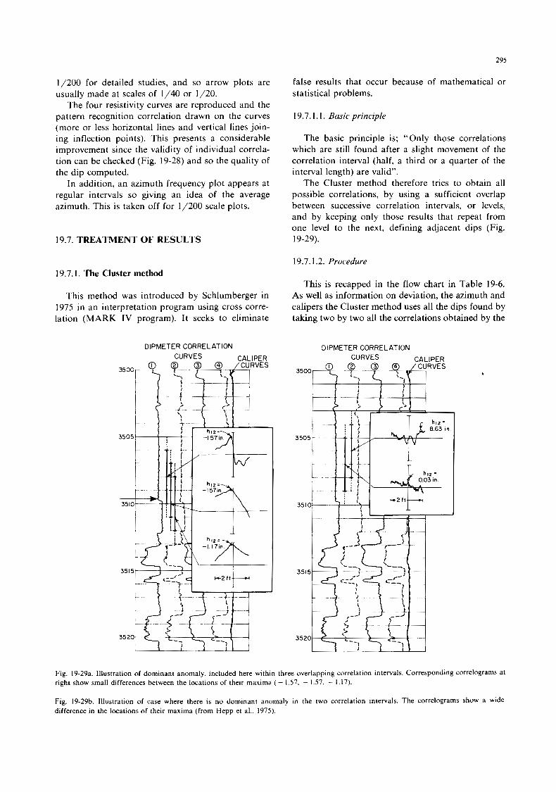
295
1/200 for detailed studies, and so arrow plots are usually made at scales of 1/40 or 1/20.
The four resistivity curves are reproduced and the pattern recognition correlation drawn on the curves (more or less horizontal lines and vertical lines join- ing inflection points). This presents a considerable improvement since the validity of individual correla- tion can be checked (Fig. 19-28) and so the quality of the dip computed.
In addition, an azimuth frequency plot appears at regular intervals so giving an idea of the average azimuth. This is taken off for 1/200 scale plots.
19.7. TREATMENT OF RESULTS
19.7.1. The Cluster method
This method was introduced by Schlumberger in 1975 in an interpretation program using cross corre- lation (MARK IV program). I t seeks to eliminate
DIPMETER CORRELATION
false results that occur because of mathematical or statistical problems.
19.7.1.1. Basic principle
The basic principle is; “Only those correlations which are still found after a slight movement of the correlation interval (half, a third or a quarter of the interval length) are valid”.
The Cluster method therefore tries to obtain all possible correlations, by using a sufficient overlap between successive correlation intervals, or levels, and by keeping only those results that repeat from one level to the next, defining adjacent dips (Fig. 19-29).
19.7.1.2. Procedure
This is recapped in the flow chart in Table 19-6. As well as information on deviation, the azimuth and calipers the Cluster method uses all the dips found by taking two by two all the correlations obtained by the
DIPMETER CORRELATION
Fig. 19-29a. Illustration of dominant anomaly, included here within three overlapping correlation intervals. Corresponding correlograms at right show small differences between the locations of their maxima ( - 1.57. - 1.57. - 1.17).
Fig. 19-29b. Illustration of case where there is no dominant anomaly in the two correlation intervals. The correlograms show a wide difference in the locations of their maxima (from Hepp et al., 1975).
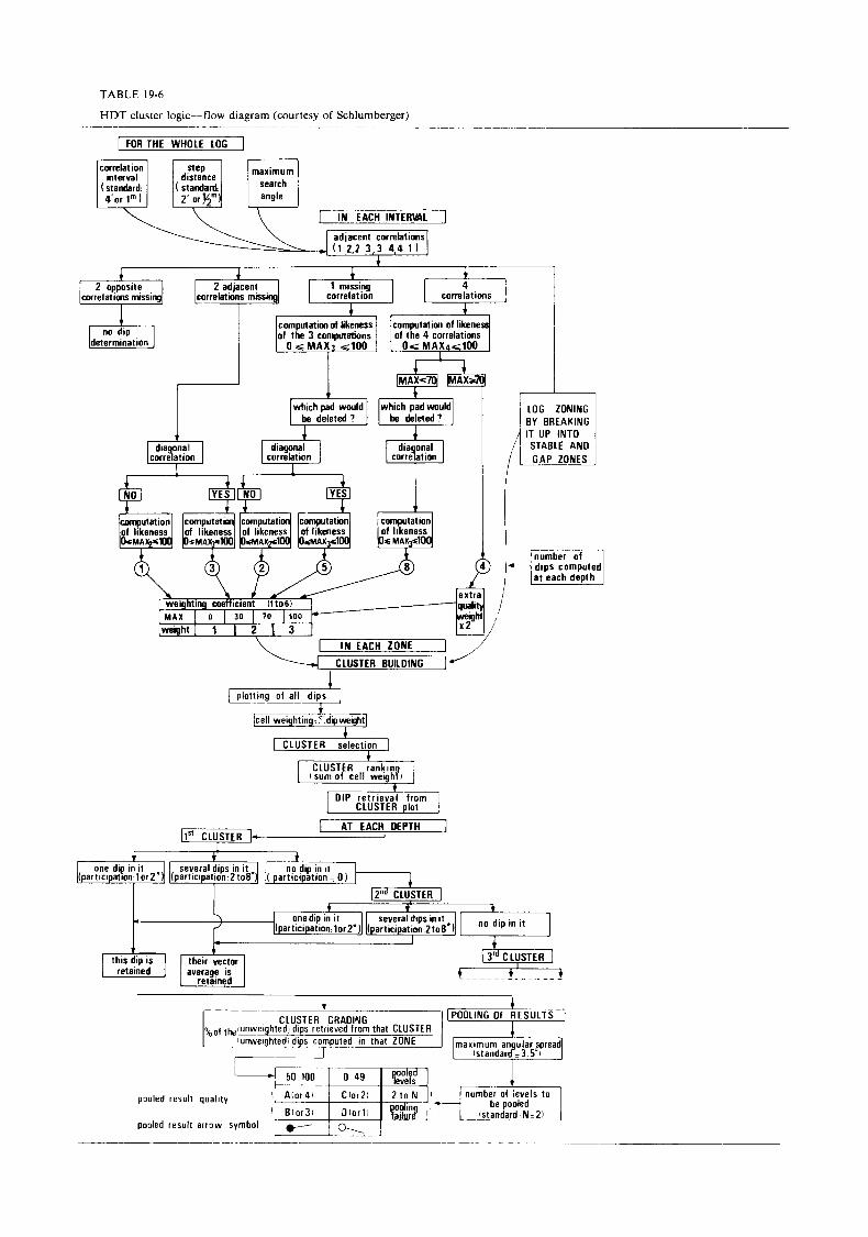
TABLE 19-6
HDT cluster logc--flow diagram (courtesy of Schlumberger) - _ _ _ ~ -~
I FORTHE WHOLE LOG 1 --- correlation dep 1 , interval 1 distance 1 1 m:ttr I
standard: standard
adjacent correlations ( 1-2.2 . 3 , 3 ~ 4,4- 1 I
correlation correlations
1
, - . -. . -. . . . . . - - ,
corr iat ion correlation corre tion GAP ZONES
i 1 I I
unnputation cornputat. computati cornputatin 01 likeness of likeness of likeness of likeness L M A % < J bSMAXpIl["l ~8MAX.p~~ L d A X 3 < 1 4 kzig (4 2 5 a
weighting Qpp/ coefficient (1 1061
MAX I 0 I 30 I 70 I100
1 2 1 3 -1
CLUSTER BUILDING I I
number of dips computed
/cell weighting,Zdipwem$t] 4
1 CLUSTER selection J + CLUSTER rankin [ I sum of cell weigh?) 1
1
CLUSTER plot DIP retr ieval from
1 AT EACH OEPTH 1 11'' CLUSTER
I
I
i CLUSTER GRADING
th iKweightedl dips retrieved lrom that CLUSTER lunweightedl dips computed in that
i
297
TABLE 19-7
Example of results from an existing dipmeter program used as input to cluster (from Hepp et al., 1975)
D E P T H W E L L TOOL ( F E E T ) CALIPERS 7 CURVE DISPLACEMENTS DEVIATION ORIENTATION
lD13 D24 H12 H23 H34 H41 H13 H24 MAX DEV DVAZ P A Z RB (INCHES) IINCHES) (DEGREES) (DECREES)
3836 8.9 8.4 -0.34 -0.99 0.39 0.79 2 :k 57 2.3 7 202 195 3834 8.8 8.4 -0.29 4.20 -0.29 1.26 -1.91 46 2.4 7 203 196 3832 8.8 8.4 3.58 1.46 -0.45 10 2.4 5 203 198 3830 8.8 8.4 -2.97 1.42 -0.06 1.07 -2.22 24 2.4 3 202 199 3828 8.8 8.4 -3.24 1.77 0.74 1.52 31 2.5 2 200 198 3826 8.7 8.4 -3.21 -0.40 1.21 0.49 -3.35 3 6 2.5 3 201 198 3824 8.6 8.4 -0.90 -0.28 1.10 0.37 0.73 3 8 2.5 4 204 200 3822 8.5 8.4 -1.04 -0.04 1.12 0.51 0.94 3 5 2.6 4 202 198 3820 8.6 8.2 -4.45 5.10 1.21 3.22 -3.20 40 2.7 3 196 193 3818 8.5 8.1 0.63 0.11 6.88 -0.07 -0.20 22 2.6 3 191 188 3816 8.5 8.4 0.70 0.04 0.60 27 2.5 5 191 185 3814 8.6 8.5 -0.90 1.04 -0.80 0.11 30 2.4 4 188 183 3812 8.6 8.4 -0.57 0.97 0.62 25 2.3 360 185 184 3810 8.5 8.3 0.16 0.99 0.87 -1.92 :% 23 2.2 359 182 183 3808 8.5 8.2 0.79 -1.16 -0.17 24 2.1 360 177 177
3 7 2.1 359 172 173 3806 8.6 8.2 -2.42 1.56 1.27 -0.11 3804 8.6 8.3 0.19 -4.47 -4.16 1 4 2.1 358 171 172
NO CORRELATION 2.0 1 174 172 3802 8.6 8.5 3802 8 . 6 . 8.5 NO CORRELATION 2.0 1 174 172 3800 8 . 4 ' 8.6 -5.80 -6.00 0.38 -9.13 35 2.0 360 183 182 3798 8.0 8.3 5.49 0.93 -2.31 3 7 2.0 359 192 192 3796 8.2 8.2 0.81 0.11 -0.78 1.16 14 2.0 2 194 192
TABLE 19-8
Example of zoning defined from the displacements (from Hepp et al., 1975)
ADJACENT-CURVE DISPLACEMENTS
r I
( F E E T ) (INCHES) (DEGR.1
A
DEPTH H12 H23 H34 HI1 P A 2
OPEN ZONE 3858 3 . 7 1 -0.69 3856 0.81 -0.65 3854 0.97 -0.43 3852 0.92 -0.46 3850 0.77 -0.20 3848 0.70 -0.12 3846 -0.31 STABLE ZONE 3844 0.32 -0.58 3842 0.11 -0.79 3840 -0.04 -0.93 3838 -0.25 -1.03 3836 -0.34 -0.99 OPEN ZONE 3834 -0.29 4.20 3832 3.58 1.46 3830 -2.97 1.42 3828 -3.24 3826 -3.21 -0.40 3824 -0.90 -0.28 3822 -1.04 -0.04 3820 -4.45 5.10 3818 0.63 0.11 3816 0.70 0.04 OPEN ZONE 3814 -0.90 1.04 3812 -0.57 0.97 3810 0.16 0.99 3808 3806 -2.42 1.56 3804 0.1 9 3802 3800 -5.80 -6.00 3798 5.49 3796 0.81 0.11
3.43 -3.27 181 -0.90 0.78 192 -1.24 -0.70 189 -1.39 182 -1.45 0.59 178 -4.46 176 -4.82 180
-0.37 0.45 195 -0.34 0.36 205
0.65 208 0.44 0.73 205 0.39 0.79 202
-0.29 1.26 233 203
-0.06 1.07 LO2 1.77 0.74 200 1.21 0.49 201 1.10 0.37 204 1.12 0.51 202 1.21 3.22 196 6.88 -0.07 191
191
-0.80 188 I85
0.87 -1.92 182 0.79 -1.16 177 1.27 -0.11 172
-4.47 171 174
0.38 -9.13 183 0.93 -2.31 192
-0.78 194
9
cross-correlation programs (2, 3 or 4 adjacent correla- tions and one diagonal). Then the displacement list- ing (Table 19-7) is divided into zones corresponding to given depth intervals.
The consecutive displacements between the same two electrodes are studied with the objective of iden- tifying stable intervals and so grouping levels into stable or unstable zones.
Pad No4 0 Weight = I + Weight = 2
\Pad No I F X I '
Cluster'- E~ i + ++
No2 a + +
\ + I + + /'
i Y
Pad No 2
Fig, 19-30. Plot of dip results on two-dimensional map (scalings removed). Two clusters are circled, and a near cluster is indicated in a dashed circle. (from Hepp et al., 1975).
298
TABLE 19-9
Cluster output listing (from Hepp et al., 1975)
DEPTH DIP DIP D E V D E V I A Z M A Z M
I
I
I
I * * * I
I
I
I
I
* * I
I
I
I
I
I I
I
I
I
* I
I
I
I
I
I
t
I
3 0 9 6 6 . 4 222 2.1 3894 8 . 0 150 2 .1 3092 8.5 1 9 0 2 .1 38991 11.4 224 2.1 5 R a 8 5.1 101 2.2 3086 3.9 i'idd 2.1 3684 7.7 Z R 6 2.1 30e2 7.1 196 2.2 3908 1 . 6 164 2.2 5 0 1 6 18.6 143 2.9 307s 14.9 1 0 6 L . 4 3 0 7 2 13 .5 151 2.3 5 0 7 n i5.e 152 2 . 3 3 6 6 8 2 9 . 7 2 9 1 2.4 3866 12.8 1 5 3 2.1) 3 0 6 0 15 ,a 1 6 5 P.U 3662 11.3 117 2 . U 3856 1 R . d 119 2 . 1 3 8 5 4 18.3 1 3 9 2.0 3 8 5 2 1B.h 1 2 9 2 . 0 3 0 5 3 10.1 1 2 2 2.m 30110 6 . 5 1 3 5 2.0 3 0 0 4 7.7 1 1 2 2.0 3802 6.1 1 1 5 2 . 1 3046 6 . 0 8 5 2 .2 3 0 3 0 6 .4 6 2 2 . 5 3 8 3 6 6 . 4 5 9 2 . 3 3 0 3 8 1R.7 24 2.4 3 0 2 8 23.0 3 0 6 2.5
3824 6 . 6 3 5 3 2.5 3 8 2 2 ? , 3 3 0 5 ?.b 3814 1 2 . B 2 6 2 2.4 3 0 1 2 10.8 243 2.3 3018 11.8 2 5 0 2 . 2 38R8 12.5 2 5 1 2 .1 JeIF6 18.1 2 5 8 2 .1 3 7 9 0 9 .6 244 2.0
3 1 8 2 (F.5 34b 2.0
3 e 2 6 0.4 354 2 .5
3 1 8 8 5.2 257 z.co
1 z 4 J 3 4 z 0 2 9 4 3 1 1 1 1 1 9
1 2 14 16 17 16 14 1 1
7 7 3 2 3 1 4 4
Sb@ 359 Jb0 359 3 6 0
0 0
D13 D24 LO Q R C C E P A R MAX S P D GIC C O R I
C C C A A A
I. A A A D
I* I) 0 0 D
0 D
I. A A A A C A A A
I. A I* A
D D D 8 I) D D
I* D 0 D
I* A A A
e
10 l(d 10 10 10 10 1 0 10 18 10 10 10 1 0 2 0 1 0 10 10 10 10 10 10 10 1 0 10 l(d 10 10 10 20 10 10 10 l(d 10 10 10 10 10 10 10
1 I z e 7 8 8 8 8 1 8 5 0 2 S 1 1 8 S I 8 1 8 8 S 8 b 1 1 2 8 8 1 3 2 S 1 b I S
I0 I 4 27 33 2 9 56 11 S 1 5 1 EZ
4 Zb J l
25 1 6 3 t 4 0 17 I 8 IS 2 1 Sb 4 9 1s e9 57 ae 51 16 34 1s 10 ES 23 I 3 1 7 1 b 49 I b
J e
I I I I I
I I I . I I I I
I I
I . I *
I I I I I I .
I * I I 0 c . c
0 I . . I I * I
i I I 9
Fig. 19-31. Dipmeter results before and after using Cluster (from Hepp et al., 1975).
299
ORRELRTLON CURYE
By a stable zone we mean an interval in depth in which successive displacements (one level to the next) do not differ by more than a certain percentage (Fig. 19-29 and Table 19-8) ( i f not the zone is open or unstable).
For each level of each zone so defined as stable or open, each of the intermediate dips is calculated by grouping two by two the displacements (the number of combinations is limited to eight).
Each intermediate dip so determined is given a
miw
FROM THE CLUSTER
POOLED RRREN PLO
2 L E V E L S PllOLEC
3 . 5 DEGREES S D L I
BLACK ARROWS RRE
4 FT X 2 FT 35
REFERENCE 120-14
PROC
HEN
ANC
POOL
EGR
70.1
830C
940C
3500
360C
970c
3800
3900
D I P REflOYEIl
weight (from 1 to 3) according to the quality of the correlation. The weight is doubled if the level has a good planarity (and thus a good closure as well).
For a given zone, each weighted intermediate dip is plotted on a Schmidt plot. When dips fall at the same place their weights are added.
The plot is analyzed to identify dip concentrations or groupings * of sufficient weight or density (Fig.
The final dip retained for a level is selected only from those that fall in the grouping or near to it. This selection is not very restrictive in order not to prevent the production of red or blue patterns.
Each final dip selected is given with a classifica- tion that depends on the quality of the cluster or grouping in which it falls and on the number of dips at the level that fall in the group (which depends on the closure, the planarity and stability of the adjacent levels).
These dips are set out in a listing with their quality (Table 19-9).
Simultaneously the program puts together the dips from adjacent stable levels in one average dip vector that is output in a separate file. The arrow plot is made from this file. This reduces the large density of arrows on the log and eliminates duplication of the same dip result arising from the presence of the same dominant anomaly in successive correlation intervals that overlap. The file also serves as the basis for the results listing given to a client (see example in Table
19-30).
19-9).
EON
19.7.1.3. Critique of the Cluster method
It has the advantage of eliminating noise as the comparison of processing with and without the Clus- ter method show (Fig. 19-31).
However, there is the risk of eliminating dips considered as noise when they really do correspond to an actual phenomenon and so are likely to help in interpretation of the arrow plot.
19.7.2. Determination of structural dip (Diptrend)
A statistical study of the dips determined by Clus- ter, made in intervals more or less large and homoge- neous, showing dips constant in magnitude and azimuth corresponding to parallel boundaries without current influence, permits the determination of structural dip for these intervals.
19.7.3. Dip-removal
Knowing the structural dip it can be removed from the dip values (vector subtraction). Ths leads to
* i.e. the participation of each level to the grouping (column PAR on the results listed in Table 19-9). Fig. 19-32. Example of result after dip-removal.
300
1
-. Fig. 19-33. Example of Fracture Identification Log (F.I.L.) (courtesy of Schlumberger).
a new arrow plot that can be used to make a study of sedimentary features and to define the direction of transport (Fig. 19-32).
DIPS
RESlSTlVlll N
C&L.IIPER 2 -
I -- 20 W + E
S
CALIPER 1
1 - -20
d lo-
I
I 1 t I 1 i I I I I 1 I I
1 4
4
.d 5 8 60' 70'
SIVE I :'I s y : I ALE -SAND MIN6TIONS
ND-SHALE NATIONS
,ALE STRE
~
CORRELATIONS
RESISTIVITY
CURVES
Fig. 19-34. Example of Sedimentary Features seen on a Geodip (courtesy of Schlumberger).
deformation such as faults, folding, etc.
tures. (F.I.L. Presentation, Fig. 19-33.) The resistivity curves can be used to detect frac-
19.8.2. Sedimentary applications 19.8. APPLICATIONS
These are of three types.
19.8.1. Tectonic or structural applications
Dip measurements are fundamentally used to de- fine regional or structural dip, but also to detect structural dip anomalies associated with structural
A dipmeter, especially when it has been processed with GEODIP, gives an indication of sedimentary features present in the interval and consequently an idea of the depositional processes: bedding type (flaser, wavy, lenticular bedding, parallel boundaries), current features (cross-bedding), and graded bedding.
In addition, a study of the original resistivity curves and of the dips related to each correlation
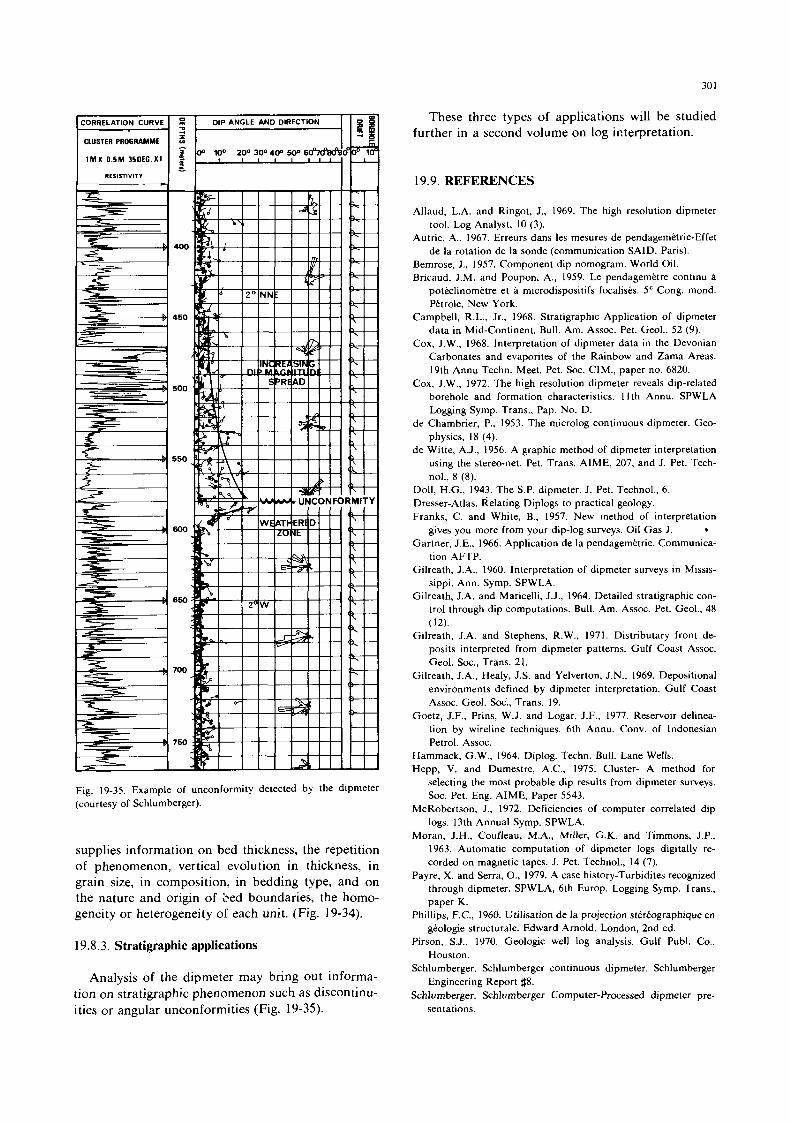
30 1
CORRELATION CURVE
CLUSTER PROGRAMME I 1MX 0.5M 3 5 O E G . X l
DIP ANGLE AND DIRECTION
00 10° ZOO 30°400 5O0 6O"lBaBsO
RESISTIVITY
El*' I I
Fig. 19-35. Example of unconformity detected by the dipmeter (courtesy of Schlumberger).
supplies information on bed thickness, the repetition of phenomenon, vertical evolution in thickness, in grain size, in composition, in bedding type, and on the nature and origin of bed boundaries, the homo- geneity or heterogeneity of each unit. (Fig. 19-34).
19.8.3. Stratigraphic applications
Analysis of the dipmeter may bring out informa- tion on stratigraphic phenomenon such as discontinu- ities or angular unconformities (Fig. 19-35).
These three types of applications will be studied further in a second volume on log interpretation.
19.9. REFERENCES
Allaud, L.A. and Ringot, J., 1969. The high resolution dipmeter
Autric, A., 1967. Erreurs dans les mesures de pendagemetrie-Effet
Bemrose, J., 1957. Component dip nomogram. World Oil. Bricaud, J.M. and Poupon, A,, 1959. Le pendagemetre continu a
poteclinometre et a microdispositifs focalises. 5 e Cong. mond. Petrole, New York.
Campbell, R.L., Jr., 1968. Stratigraphic Application of dipmeter data in Mid-Continent. Bull. Am. Assoc. Pet. Geol., 52 (9).
Cox, J.W., 1968. Interpretation of dipmeter data in the Devonian Carbonates and evaporites of the Rainbow and Zama Areas. 19th Annu Techn. Meet. Pet. SOC. CIM., paper no. 6820.
Cox, J.W., 1972. The high resolution dipmeter reveals dip-related borehole and formation characteristics. 1 1 th Annu. SPWLA Logging Symp. Trans., Pap. No. D.
d e Chambrier, P., 1953. The microlog continuous dipmeter. Geo- physics, 18 (4).
d e Witte, A.J., 1956. A graphic method of dipmeter interpretation using the stereo-net. Pet. Trans. AIME, 207, and J. Pet. Tech- no]., 8 (8).
tool. Log Analyst, 10 (3).
de la rotation de la sonde (communication SAID, Paris).
Doll, H.G., 1943. The S.P. dipmeter. J. Pet. Technol., 6. Dresser-Atlas. Relating Diplogs to practical geology. Franks, C. and White, B., 1957. New method of interpretation
gives you more from your dip-log surveys. Oil Gas J. Gartner, J.E., 1966. Application de la pendagemetrie. Communica-
tion AFTP. Gilreath, J.A., 1960. Interpretation of dipmeter surveys in Missis-
sippi. Ann. Symp. SPWLA. Gilreath, J.A. and Maricelli, J.J., 1964. Detailed stratigraphic con-
trol through dip computations. Bull. Am. Assoc. Pet. Geol., 48
Gilreath, J.A. and Stephens, R.W., 1971. Distributary front de- posits interpreted from dipmeter patterns. Gulf Coast Assoc. Geol. SOC., Trans. 21.
Gilreath, J.A., Healy, J.S. and Yelverton, J.N., 1969. Depositional environments defined by dipmeter interpretation. Gulf Coast Assoc. Geol. Soc., Trans. 19.
Goetz, J.F., Prins, W.J. and Logar, J.F., 1977. Reservoir delinea- tion by wireline techniques. 6th Annu. Conv. of Indonesian Petrol. Assoc.
*
(12).
Hammack, G.W., 1964. Diplog. Techn. Bull. Lane Wells. Hepp, V. and Dumestre, A.C., 1975. Cluster- A method for
selecting the most probable dip results from dipmeter surveys. SOC. Pet. Eng. AIME, Paper 5543.
McRobertson, J., 1972. Deficiencies of computer correlated dip logs. 13th Annual Symp. SPWLA.
Moran, J.H., Coufleau, M.A., Miller, G.K. and Timmons, J.P., 1963. Automatic computation of dipmeter logs digitally re- corded on magnetic tapes. J. Pet. Technol., 14 (7).
Payre, X. and Serra, 0.. 1979. A case history-Turbidites recognized through dipmeter. SPWLA, 6th Europ. Logging Symp. Trans., paper K.
Phillips, F.C., 1960. Utilisation de la projection stereographique en geologie structurale. Edward Arnold, London, 2nd ed.
Pirson, S.J., 1970. Geologic well log analysis. Gulf Publ. Co., Houston.
Schlumberger. Schlumberger continuous dipmeter. Schlumberger Engineering Report #8.
Schlumberger. Schlumberger Computer-Processed dipmeter pre- sentations.

302
Schlumberger. (Surenco et L.A. Allaud) Use of stereographic pro-
Schlumberger, 1970. Fundamentals of dipmeter interpretation. New
Schlumberger, I98 1. Dipmeter interpretation. Fundamentals. Selley. R.C.. 1978. Ancient Sedimentary Environments. Chapman
jection in dipmeter analysis.
York.
and Hall, London.
Selley, R.C., 1979. Dipmeter and log motifs in North Sea sub- marine-fan sands. Bull. Am. Assoc. Pet. Geol., 63 ( 6 ) .
Vincent, Ph., Gartner, J.E. and Attali, G., 1977. Geodip: an approach to detailed dip determination using correlation by pattern recognition. 52nd Annu. Fall Techn. Conf. SPE of AIME, Paper 6823.
Welex, 1970. Dip log Interpretation.
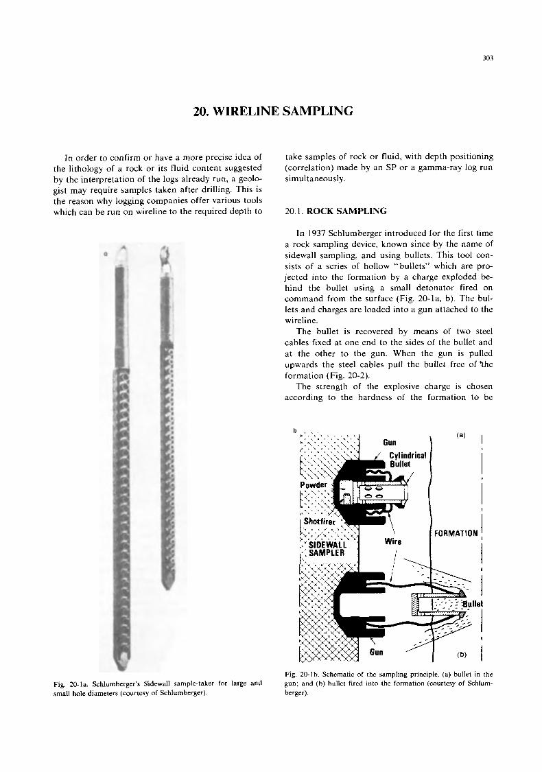
303
20. WIRELINE SAMPLING
In order to confirm or have a more precise idea of the lithology of a rock or its fluid content suggested by the interpretation of the logs already run, a geolo- gist may require samples taken after drilling. This is the reason why logging companies offer various tools which can be run on wireline to the required depth to
Fig. 20-la. Schlumberger’s Sidewall sample-taker for large and small hole diameters (courtesy of Schlumberger).
take samples of rock or fluid, with depth positioning (correlation) made by an SP or a gamma-ray log run simultaneously.
20.1. ROCK SAMPLING
In 1937 Schlumberger introduced for the first time a rock sampling device, known since by the name of sidewall sampling, and using bullets. This tool con- sists of a series of hollow “bullets” which are pro- jected into the formation by a charge exploded be- hind the bullet using a small detonator fired on command from the surface (Fig. 20-la, b). The bul- lets and charges are loaded into a gun attached to the wireline.
The bullet is recovered by means of two steel cables fixed at one end to the sides of the bullet and at the other to the gun. When the gun is pulled upwards the steel cables pull the bullet free of ’the formation (Fig. 20-2).
The strength of the explosive charge is chosen according to the hardness of the formation to be
& I . . . I Shotfii . . . r
rical
Fig. 20-lb. Schematic of the sampling principle. (a) bullet in the gun; and (b) bullet fired into the formation (courtesy of Schlum- berger).
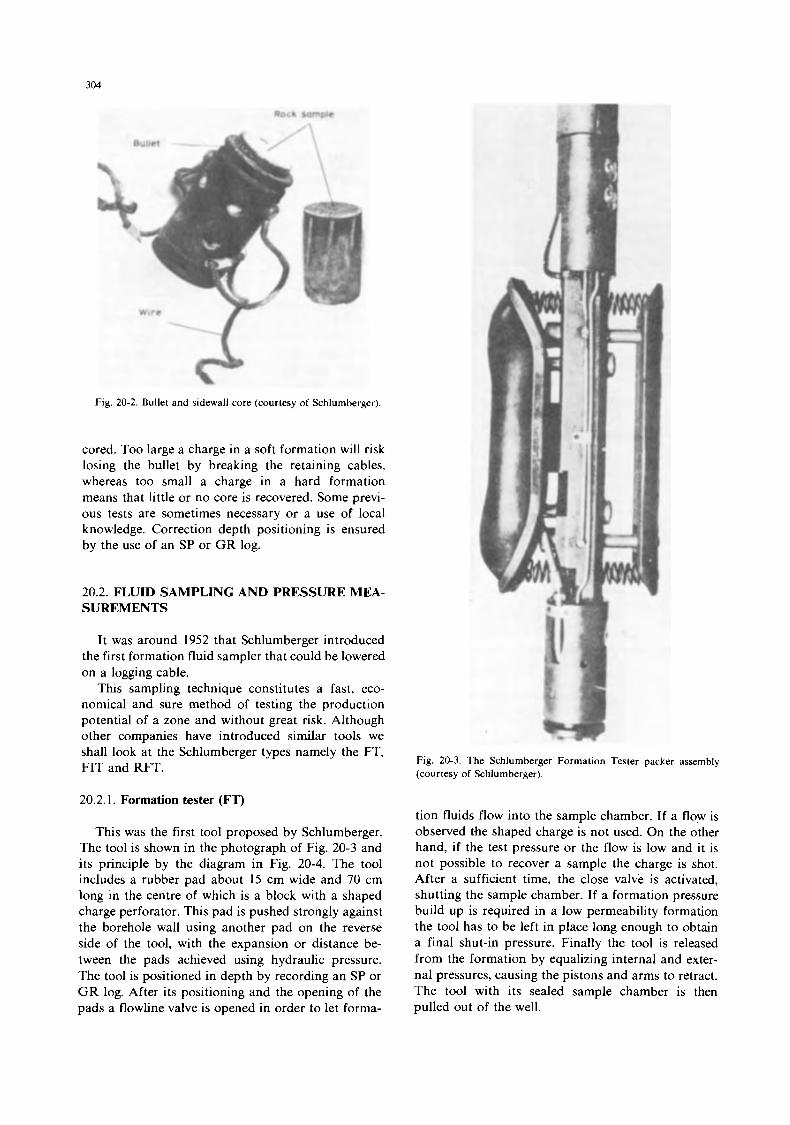
304
Fig. 20-2. Bullet and sidewall core (courtesy of Schlumberger).
cored. Too large a charge in a soft formation will risk losing the bullet by breaking the retaining cables, whereas too small a charge in a hard formation means that little or no core is recovered. Some previ- ous tests are sometimes necessary or a use of local knowledge. Correction depth positioning is ensured by the use of an SP or GR log.
20.2. FLUID SAMPLING AND PRESSURE MEA- SUREMENTS
It was around 1952 that Schlumberger introduced the first formation fluid sampler that could be lowered on a logging cable.
This sampling technique constitutes a fast, eco- nomical and sure method of testing the production potential of a zone and without great risk. Although other companies have introduced similar tools we shall look at the Schlumberger types namely the FT, FIT and RFT.
20.2.1. Formation tester (FT)
This was the first tool proposed by Schlumberger. The tool is shown in the photograph of Fig. 20-3 and its principle by the diagram in Fig. 20-4. The tool includes a rubber pad about 15 cm wide and 70 cm long in the centre of which is a block with a shaped charge perforator. This pad is pushed strongly against the borehole wall using another pad on the reverse side of the tool, with the expansion or distance be- tween the pads achieved using hydraulic pressure. The tool is positioned in depth by recording an SP or G R log. After its positioning and the opening of the pads a flowline valve is opened in order to let forma-
Fig. 20-3. The Schlumberger Formation Tester packer assembly (courtesy of Schlumberger).
tion fluids flow into the sample chamber. If a flow is observed the shaped charge is not used. On the other hand, if the test pressure or the flow is low and it is not possible to recover a sample the charge is shot. After a sufficient time, the close valve is activated, shutting the sample chamber. If a formation pressure build up is required in a low permeability formation the tool has to be left in place long enough to obtain a final shut-in pressure. Finally the tool is released from the formation by equalizing internal and exter- nal pressures, causing the pistons and arms to retract. The tool with its sealed sample chamber is then pulled out of the well.
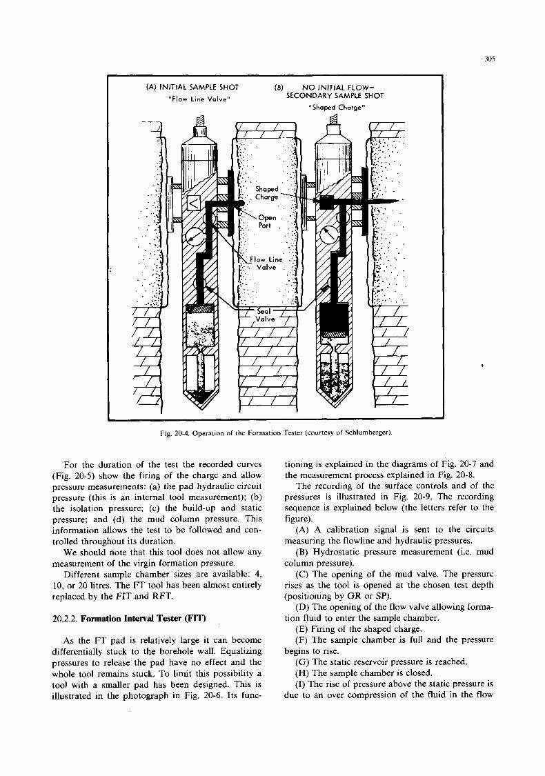
305
(A) INITIAL SAMPLE SHOT (B) NO INITIAL FLOW- SECONDARY SAMPLE SHOT
"Shaped Charge" "Flow Line Valve"
.
~~ ~~
Fig. 20-4. Operation of the Formation Tester (courtesy of Schlumberger).
For the duration of the test the recorded curves (Fig. 20-5) show the firing of the charge and allow pressure measurements: (a) the pad hydraulic circuit pressure (this is an internal tool measurement); (b) the isolation pressure; (c) the build-up and static pressure; and (d) the mud column pressure. This information allows the test to be followed and con- trolled throughout its duration.
We should note that this tool does not allow any measurement of the virgm formation pressure.
Different sample chamber sizes are available: 4, 10, or 20 litres. The FT tool has been almost entirely replaced by the FIT and RFT.
20.2.2. Formation Interval Tester (FIT)
As the FT pad is relatively large it can become differentially stuck to the borehole wall. Equalizing pressures to release the pad have no effect and the whole tool remains stuck. To limit this possibility a tool with a smaller pad has been designed. This is illustrated in the photograph in Fig. 20-6. Its func-
tioning is explained in the diagrams of Fig. 20-7 and the measurement process explained in Fig. 20-8.
The recording of the surface controls and of the pressures is illustrated in Fig. 20-9. The recording sequence is explained below (the letters refer to the figure).
(A) A calibration signal is sent to the circuits measuring the flowline and hydraulic pressures.
(B) Hydrostatic pressure measurement (i.e. mud column pressure).
( C ) The opening of the mud valve. The pressure rises as the tool is opened at the chosen test depth (positioning by GR or SP).
(D) The opening of the flow valve allowing forma- tion fluid to enter the sample chamber.
(E) Firing of the shaped charge. (F) The sample chamber is full and the pressure
(G) The static reservoir pressure is reached. (H) The sample chamber is closed. (I) The rise of pressure above the static pressure is
due to an over compression of the fluid in the flow
begins to rise.
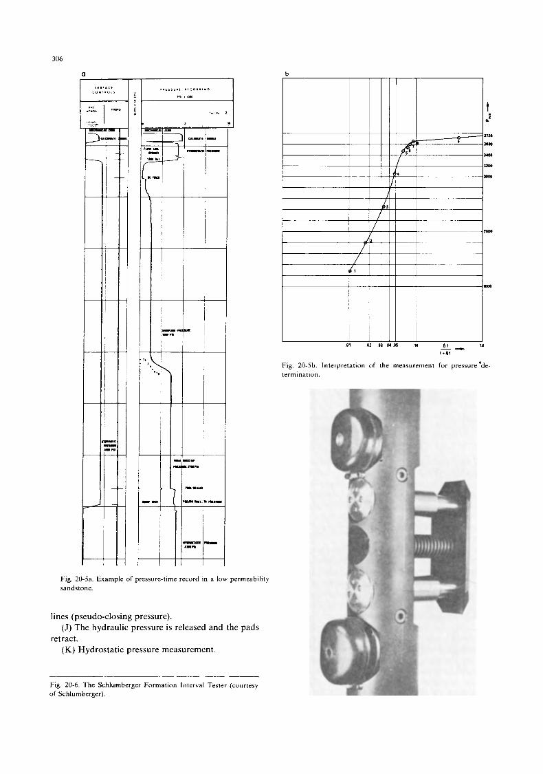
306
/ 1
!!!szEc I
V / L
02
M Y
lmN
t
Fig. 20-5a. Example of pressure-time record in a low permeability sandstone.
lines (pseudo-closing pressure).
retract. (J) The hydraulic pressure is released and the pads
(K) Hydrostatic pressure measurement.
.- ~~ __ -- __. .- --
Fig. 20-6. The Schlumberger Formation Interval Tester (courtesy of Schlumberger).
r !== t t
t l + A l
Fig. 20-5b. Interpretation of the measurement for pressure ‘de- termination.
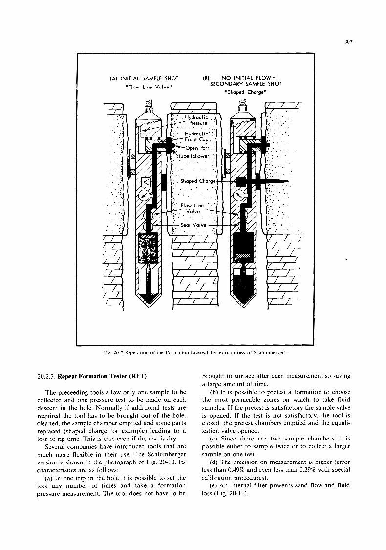
307
(A) INITIAL SAMPLE SHOT (B) NO INITIAL FLOW - SECONDARY SAMPLE SHOT
"Shaped Charge" "Flow Line Valve"
I Fig. 20-7. Operation of the Formation Interval Tester (courtesy of Schlumberger).
20.2.3. Repeat Formation Tester (RFT)
The preceeding tools allow only one sample to be collected and one pressure test to be made on each descent in the hole. Normally if additional tests are required the tool has to be brought out of the hole, cleaned, the sample chamber emptied and some parts replaced (shaped charge for example) leading to a loss of rig time. This is trh: even if the test is dry.
Several companies have introduced tools that are much more flexible in their use. The Schlumberger version is shown in the photograph of Fig. 20-10. Its characteristics are as follows:
(a) In one trip in the hole it is possible to set the tool any number of times and take a formation pressure measurement. The tool does not have to be
brought to surface after each measurement so saving a large amount of time.
(b) It is possible to pretest a formation to choose the most permeable zones on which to take fluid samples. If the pretest is satisfactory the sample valve is opened. If the test is not satisfactory, the tool is closed, the pretest chambers emptied and the equali- zation valve opened.
(c) Since there are two sample chambers it is possible either to sample twice or to collect a larger sample on one test.
(d) The precision on measurement is higher (error less than 0.49% and even less than 0.29% with special calibration procedures).
(e) An internal filter prevents sand flow and fluid loss (Fig. 20-1 1).
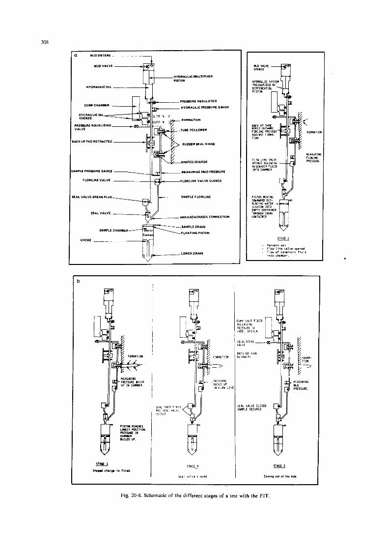
308
a MUDENTERS
MUDVALVE -
HYDRAULIC MULTIPLIER
HYDRAULIC OIL
PRESSURE REGULATOR
DUMP CHAMBER HYDRAULIC PRESSURE GAUGE
HYDRAULIC OIL CHOKES
PRESSURE EOUAL1ZING VALVE TUBE FOLLOWER
RUBBERSEAL RlNQS BACK-UP PAD RETRACTED
SHAPED CHARGE
SAMPLE PRESSURE GAUGE MEASURING MUD PRESSURE
FLOWLINE VALVE -FLOWLINE VALVE CLOSED
SEAL VALVE BREAK PLUG SAMPLE FLOWLINE
AMERADAIHUGEL CONNECTION SEAL VALVE I
SAMPLE DRAIN
FLOATING PISTON SAMPLE CHAMBER
-L LOWER DRAIN
UJO VALVE OPENED
HYDRWLlC SVST PRESSURIZED BY
J/ \\
MOVED WTYUlO FORCING AGAINST PICKLES FOIWA- F O R R T I O
LIEASURINI FLtlYlNG PRESSURE FLOY L I N E VALVE
OPENED ALLOYIHG RESERVOIR F L U 1 0 INTO CHAMBER
PISTON M O V I f f i DOYNURO D I S - PLACING YATER - CUSHION l l l T 0 EMPTY CONTAINER THROUGH CHOKE CONTAINER
w STAGE 2 -
- Packers s e t - - Flow o f r e s e r v o t v f l u i d
Flow 1 inc v a l v e opened
i n t o Chdrber. '
S I A L SHOT F l R E O 4NO S f A L VALVL Ltostn
S e a l v a l v e c l o s e d
.
M IUMP SHOT FlREO 3 E L E A S I H G
i Y O R S Y S T E M w s s u R i of
FORR-
iOUAL I 1 ING VALVE
BACK UP SHOE RITRACTS
ME ASUR I NG UJD PRESSURE
SEAL VALVE CLOSED SAMPLE SLCURLO
Fig. 20-8. Schematic of the different stages of a test with the FIT.
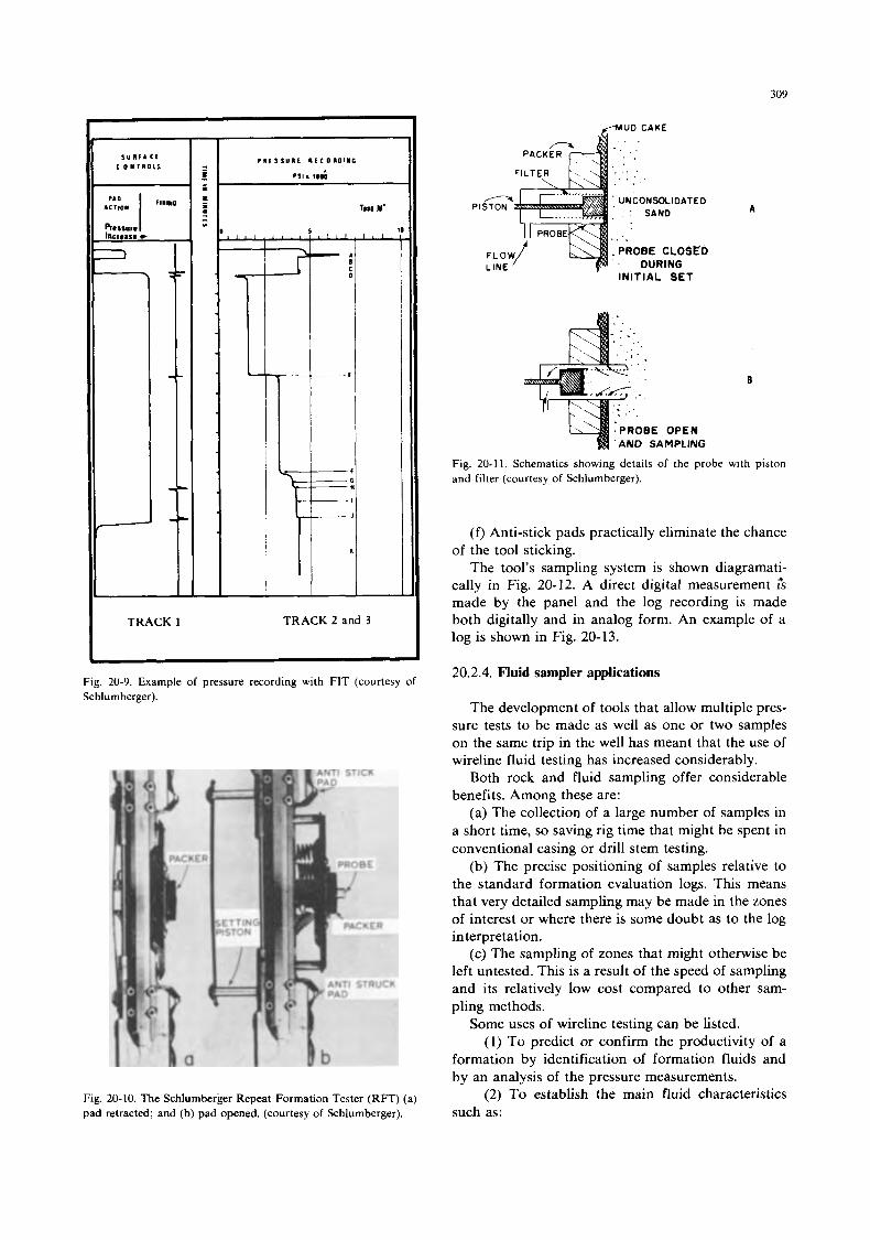
309
I: TRACK 1 TRACK 2 and 3
Fig. 20-9. Example of pressure recording with FIT (courtesy of Schlumberger).
Fig. 20-10. The Schlumberger Repeat Formation Tester (RFT) (a) pad retracted; and (b) pad opened. (courtesy of Schlumberger).
A U D CAKE
PACK
, ' . . . ' UNCONSOLIDATED A
A . SAND PISTON
I L ..,.... !
.. .
. PROBE CLOSED ' DURING
INITIAL SET
'r LINE
B
Fig. 20-11. Schematics showing details of the probe with piston and filter (courtesy of Schlumberger).
(f) Anti-stick pads practically eliminate the chance of the tool sticking.
The tool's sampling system is shown diagramati- cally in Fig. 20-12. A direct digital measurement i's made by the panel and the log recording is made both digitally and in analog form. An example of a log is shown in Fig. 20- 13.
20.2.4. Fluid sampler applications
The development of tools that allow multiple pres- sure tests to be made as well as one or two samples on the same trip in the well has meant that the use of wireline fluid testing has increased considerably.
Both rock and fluid sampling offer considerable benefits. Among these are:
(a) The collection of a large number of samples in a short time, so saving rig time that might be spent in conventional casing or drill stem testing.
(b) The precise positioning of samples relative to the standard formation evaluation logs. This means that very detailed sampling may be made in the zones of interest or where there is some doubt as to the log interpretation.
(c) The sampling of zones that might otherwise be left untested. This is a result of the speed of sampling and its relatively low cost compared to other sam- pling methods.
Some uses of wireline testing can be listed. (1) To predict or confirm the productivity of a
formation by identification of formation fluids and by an analysis of the pressure measurements.
(2) To establish the main fluid characteristics such as:
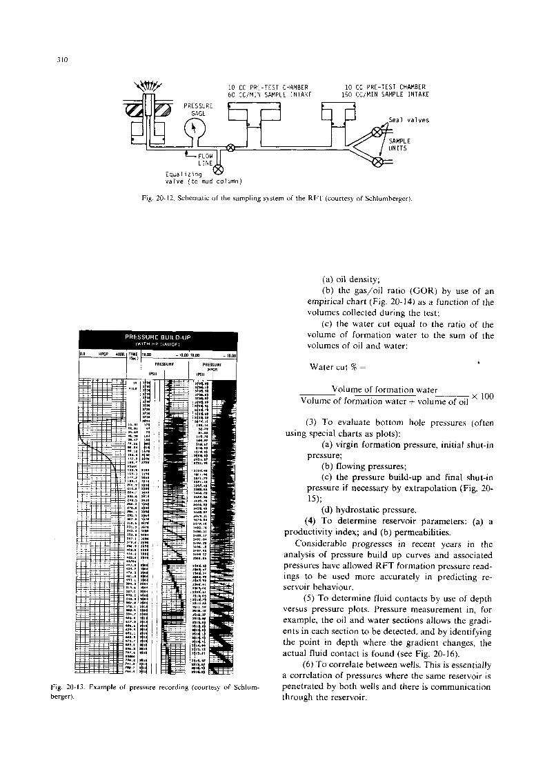
310
10 CC PRE-TEST CHAMBER 10 CC PRE-TEST CHAMBER 60 CC/MIN SAMPLE I N T A K E 150 CC/MIN SAMPLE INTAKE
v a l v e ( t o mud column)
Fig. 20-12. Schematic of the sampling system of the RFT (courtesy of Schlumberger).
(a) oil density; (b) the gas/oil ratio (GOR) by use of an
empirical chart (Fig. 20-14) as a function of the volumes collected during the test;
(c) the water cut equal to the ratio of the volume of formation water to the sum of the volumes of oil and water:
PRESSURE I I 1611 I lRll I Water cut 5% =
.
Fig. berg
20-13. Example of pressure recording (courtesy of Schlum- ;er).
Volume of formation water Volume of formation water + volume of oil x 100
(3) To evaluate bottom hole pressures (often
(a) virgin formation pressure, initial shut-in
(b) flowing pressures; (c) the pressure build-up and final shut-in
pressure if necessary by extrapolation (Fig. 20-
using special charts as plots):
pressure;
15); (d) hydrostatic pressure.
(4) To determine reservoir parameters: (a) a productivity index; and (b) permeabilities.
Considerable progresses in recent years in the analysis of pressure build up curves and associated pressures have allowed RFT formation pressure read- ings to be used more accurately in predicting re- servoir behaviour.
(5) To determine fluid contacts by use of depth versus pressure plots. Pressure measurement in, for example, the oil and water sections allows the gradi- ents in each section to be detected, and by identifying the point in depth where the gradient changes, the actual fluid contact is found (see Fig. 20-16).
(6) To correlate between wells. This is essentially a correlation of pressures where the same reservoir is penetrated by both wells and there is communication through the reservoir.
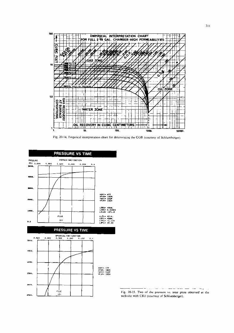
31 1
100
10
1.0
1
Fig 20-14. Empirical interpretation chart for determining the GOR (courtesy of Schlumberger)
H O R N E R TIME FUNCTION PRESSURE
(PSI) 1.000 0.800 0.600 0.400 0.200 0.0
lo@@.
0 . 0
xnxi- HTF
y n x i - SSGP XFUN- IDEN
YFUN- IDEN
LURD- 4568. LaBs- 0.04500 LSLD- -371.8
LLPL- 4214. LRPL- 4584. LTPL- -1.114 LlPL- 12.33
XPXI- S T F XFUN- IDEN Y@XII SSGP YFUN. IDEN
Fig. 20-15. Two of the pressure vs. time plots obtained at the well-site with CSU (courtesy of Schlumberger).
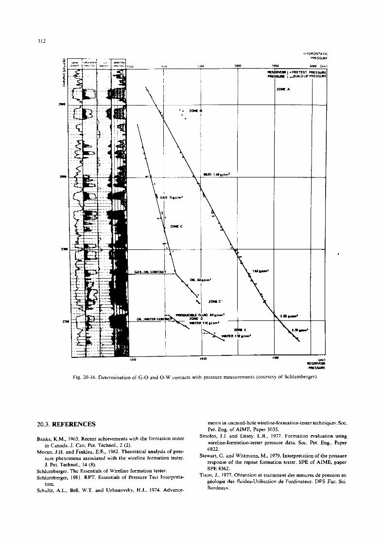
312
\
m
HYDROSTATIC
PRESYRE
Fig. 20-16. Determination of G-0 and 0 -W contacts with pressure measurements (courtesy of Schlumberger).
20.3. REFERENCES ments in uncased-hole wireline-formation-tester techniques. Soc. Pet. Eng. of AIME, Paper 5035.
Banks, K , ~ , , 1963, R~~~~
Moran, J.H. and Finklea, E.E., 1962. Theoretical analysis of pres- with the wireline formation tester,
with the formation Smolen, J.J. and Litsey, L.R., 1977. Formation evaluation using. wireline-formation-tester pressure data. Soc. Pet. Eng., Paper 6822.
Stewart, G. and Wittmann, M., 1979. Interpretation of the pressure response of the repeat formation tester. SPE of AIME, paper SPE 8362.
Tison, J., 1977. Obtention et traitement des mesures de pression en geologie des fluides-Utilisation de l'ordinateur. DES Fac. Sci. Bordeaux.
in Canada. J. Can. Pet. Technol., 2 (2).
sure phenomena J. Pet. Technol., 14 (8).
Schlumberger. The Essentials of Wireline formation tester. Schlumberger, 1981, RR. ~ ~ ~ ~ ~ ~ i ~ l ~ of pressure Test Interprets-
Schultz, A.L., Bell, W.T. and Urbanovsky, H.J., 1974. Advance- tion.
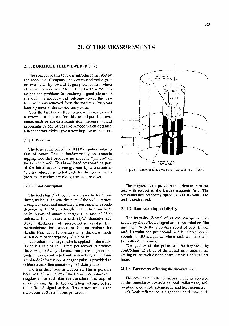
313
21. OTHER MEASUREMENTS
2 1.1. BOREHOLE TELEVIEWER (BHTV)
The concept of this tool was introduced in 1969 by the Mobil Oil Company and commercialized a year or two later by several loggmg companies which obtained licences from Mobil. But, due to some limi- tations and problems in obtaining a good picture of the wall, the industry did welcome accept t h s new tool, so it was removed from the market a few years later by most of the service companies.
Over the last two or three years, we have observed a renewal of interest for ths technique. Improve- ments made bn the data acquisition, presentation and processing by companies like Amoco which obtained a licence from Mobil, give a new impulse to this tool.
2 1.1.1. Principle
The basic principal of the BHTV is quite similar to that of sonar. This is fundamentally an acoustic logging tool that produces an acoustic “picture” of the borehole wall. This is achieved by recording part of the initial acoustic energy, sent by a transmitter (the transducer), reflected back by the formation to the same transducer working now as a receiver.
2 1.1.2. Tool description
The tool (Fig. 21-1) contains a piezo-electric trans- ducer, which is the sensitive part of the tool, a motor, a magnetometer and associated electronics. The sonde diameter is 3 3/8”, its length 12 ft. The transducer emits bursts of acoustic energy at a rate of 1500 pulses/s. It comprises a disk (1/2” diameter and 0.045” thickness) of piezo-electric crystal lead methaniobate for Amoco or lithium niobate for Sandia Nat. Lab. It operates in a thickness mode with a dominant frequency of 1.3 MHz.
An excitation voltage pulse is applied to the trans- ducer at a rate of 1500 times per second to produce the bursts, and a synchronization pulse is generated such that every reflected and received signal contains amplitude information. A trigger pulse is provided to initiate a scan line containing 485 data points.
The transducer acts as a receiver. This is possible because the low quality of the transducer reduces the ringdown time such that the transducer has stopped reverberating, due to the excitation voltage, before the reflected signal arrives. The motor rotates the transducer at 3 revolutions per second.
- PIEZOELECTRIC TRANSDUCER
Fig. 21-1. Borehole televiewer (from Zemanek et al., 1968).
The magnetometer provides the orientation of the tool with respect to the Earth’s magnetic field. The recommended recording speed is 300 ft/hour. The tool is centralized.
2 1.1.3. Data recording and display
The intensity (Z-axis) of an oscilloscope is mod- ulated by the reflected signal and is recorded on film and tape. With the recording speed of 300 ft/hour and 3 revolutions per second, a 5-ft interval corre- sponds to 180 scan lines, where each scan line con- tains 485 data points.
The quality of the prints can be improved by controlling the range of the initial amplitude, initial setting of the oscilloscope beam intensity and camera focus.
2 1.1.4. Parameters affecting the measurement
The amount of reflected acoustic energy received at the transducer depends on rock reflectance, wall roughness, borehole attenuation and hole geometry.
(a) Rock reflectance is higher for hard rock, such
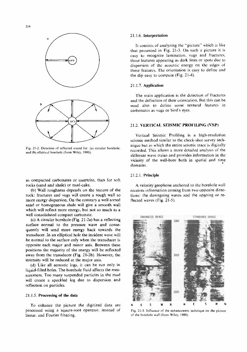
314
2 1.1.6. Interpretation
Fig. 21-2. Direction of reflected sound for: (a) circular borehole; and (b) elliptical borehole (from Wiley. 1980).
as compacted carbonates or quartzite, than for soft rocks (sand and shale) or mud-cake.
(b) Wall roughness depends on the texture of the rock: fractures and vugs will create a rough wall so more energy dispersion. On the contrary a well sorted sand or homogeneous shale will give a smooth wall which will reflect more energy, but not so much as a well consolidated compact carbonate.
(c) A circular borehole (Fig. 21-2a) has a reflecting surface normal to the pressure wave and conse- quently will send more energy back towards the transducer. In an elliptical hole the incident wave will be normal to the surface only when the transducer is opposite each major and minor axis. Between these positions the majority of the energy will be reflected away from the transducer (Fig. 21-2b). However, the intensity will be reduced at the major axis.
(d) Like all acoustic logs, i t can be run only in liquid-filled holes. The borehole fluid affects the mea- surement. Too many suspended particles in the mud will create a speckled log due to dispersion and reflection on particles.
2 1.1.5. Processing of the data
To enhance the picture the digitized data are processed using a square-root operator, instead of linear, and Fourier filtering.
I t consists of analyzing the “picture” which is like that presented in Fig. 21-3. On such a picture i t is easy to recognize lamination, vugs and fractures. these features appearing as dark lines or spots due to dispersion of the acoustic energy on the edges of these features. The orientation is easy to define and the dip easy to compute (Fig. 21-4).
2 1.1.7. Application
The main application is the detection of fractures and the definition of their orientation. But this can be used also to define some textural features in carbonates as vugs or birds eyes.
2 1.2. VERTICAL SEISMIC PROFILING (VSP)
Vertical Seismic Profiling is a high-resolution seismic method similar to the check-shot survey tech- nique but in which the entire seismic trace is digitally recorded. This allows a more detailed analysis of the different wave trains and provides information in the vicinity of the well-bore both in spatial and time domains. 9
2 1.2.1. Principle
A velocity geophone anchored to the borehole wall receives information coming from two opposite direc- tions: the downgoing waves and the upgoing or re- flected waves (Fig. 21-5).
STANOARD IMAGE EMHANCED IMAGE
1010
1020
Fig. 21-3. Influence of the enhancement technique on the picture of the borehole wall (from Wiley, 1980).
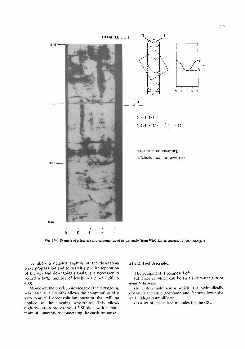
315
81 0
820
830
840
EXAMPLE 7 - 1 N E
D = 8 5 / 8 "
ANGLE = T A N
I S O M E T R I C OF
I N T E R S E C T I NG
\ /
- 1 .
FRA
T H E
)
H D -
CTI
8(
N E S W N
= 69'
JRE
I R E H O L E
H T I
r 4
N E S W N
Fig. 21-4. Example of a fracture and computation of its dip angle (from WEC Libya, courtesy of Schlumberger).
To allow a detailed analysis of the downgoing wave propagation and to permit a precise separation of the up- and downgoing signals, i t is necessary to record a large number of levels in the well (50 to 400).
Moreover, the precise knowledge of the downgoing wavetrain at all depths allows the computation of a very powerful deconvolution operator that will be applied to the upgoing wavetrains. This allows high-resolution processing of VSP data with a mini- mum of assumptions concerning the earth response.
2 1.2.2. Tool description
The equipment is composed of: (a) a source which can be an air or water gun or
even Vibroseis; (b) a downhole sensor which is a hydraulically
operated anchored geophone and features low-noise and high-gain amplifiers;
(c) a set of specialized modules for the CSU.
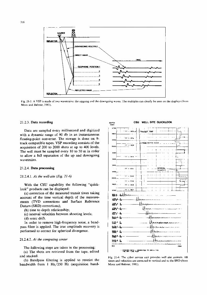
316
Fig. 21-5. A VSP is made of two wavetrains: the upgoing and the downgoing waves. The multiples can clearly be seen on the displays (from Mons and Babour, 1981).
2 1.2.3. Data recording
Data are sampled every millisecond and digitized with a dynamic range of 90 db in an instantaneous floating-point converter. The storage is done on 9- track compatible tapes. VSP recording consists of the acquisition of 200 to 2000 shots at up to 400 levels. The well must be sampled every 10 to 50 m in order to allow a full separation of the up and downgoing wavetrains.
2 1.2.4. Data processing
2 1.2.4.1. A t the well-site (Fig. 21 -6)
With the CSU capability the following "quick- look" products can be displayed:
(a) correction of the measured transit times taking account of the time vertical depth of the measure- ments (TVD corrections and Surface Reference Datum (SRD) corrections);
(b) time to depth relationship; (c) interval velocities between shooting levels; (d) sonic drift. In order to remove high-frequency noise, a band-
pass filter is applied. The true amplitude recovery is performed to correct for spherical divergence.
2 1.2.4.2. A t the computing center
The following steps are taken in the processing: (a) The shots are retrieved from the tape, edited
and stacked. (b) Bandpass filtering is applied to restrict the
bandwidth from 1 Hz/250 Hz (acquisition band-
EPTH CSU WELL SITE QUICKLOOK (feet)
-7 1 1-7 ' - - L- - I L - 1
a00
Fig. 21-6. The cyber service unit provides well site answers. All times and velocities are corrected to vertical and to the SRD (from Mons and Babour, 1981).
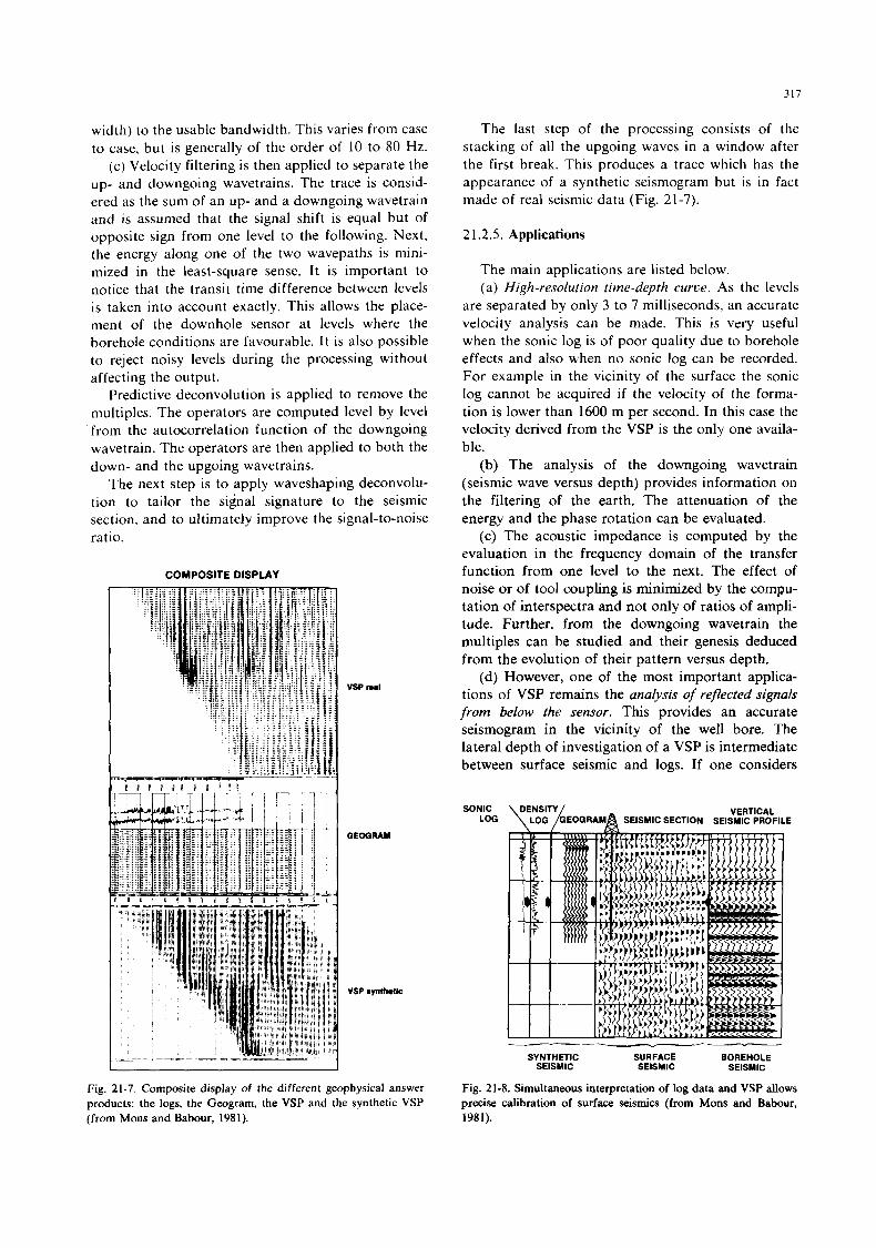
317
width) to the usable bandwidth. This varies from case to case, but is generally of the order of 10 to 80 Hz.
(c) Velocity filtering is then applied to separate the up- and downgoing wavetrains. The trace is consid- ered as the sum of an up- and a downgoing wavetrain and is assumed that the signal shift is equal but of opposite sign from one level to the following. Next, the energy along one of the two wavepaths is mini- mized in the least-square sense. I t is important to notice that the transit time difference between levels is taken into account exactly. This allows the place- ment of the downhole sensor at levels where the borehole conditions are favourable. I t is also possible to reject noisy levels during the processing without affecting the output.
Predictive deconvolution is applied to remove the multiples. The operators are computed level by level from the autocorrelation function of the downgoing wavetrain. The operators are then applied to both the down- and the upgoing wavetrains.
The next step is to apply waveshaping deconvolu- tion to tailor the signal signature to the seismic section, and to ultimately improve the signal-to-noise ratio.
COMPOSITE DISPLAY
VSP ma1
VSP a-k
Fig. 21-7. Composite display of the different geophysical answer products: the logs, the Geogram, the VSP and the synthetic VSP (from Mom and Babour, 1981).
The last step of the processing consists of the stacking of all the upgoing waves in a window after the first break. This produces a trace which has the appearance of a synthetic seismogram but is in fact made of real seismic data (Fig. 21-7).
2 1.2.5. Applications
The main applications are listed below. (a) High-resolution time-depth curve. As the levels
are separated by only 3 to 7 milliseconds, an accurate velocity analysis can be made. This is very useful when the sonic log is of poor quality due to borehole effects and also when no sonic log can be recorded. For example in the vicinity of the surface the sonic log cannot be acquired if the velocity of the forma- tion is lower than 1600 m per second. In t h s case the velocity derived from the VSP is the only one availa- ble.
(b) The analysis of the downgoing wavetrain (seismic wave versus depth) provides information on the filtering of the earth. The attenuation of the energy and the phase rotation can be evaluated.
(c) The acoustic impedance is computed by the evaluation in the frequency domain of the transfer function from one level to the next. The effect of noise or of tool coupling is minimized by the compu- tation of interspectra and not only of ratios of ampli- tude. Further, from the downgoing wavetrain the multiples can be studied and their genesis deduced from the evolution of their pattern versus depth.
(d) However, one of the most important applica- tions of VSP remains the analysis of reflected signals from below the sensor. This provides an accurate seismogram in the vicinity of the well bore. The lateral depth of investigation of a VSP is intermediate between surface seismic and logs. If one considers
SONIC LOG
VERTICAL SEISMIC PROFILE
- v -.. SYNTHETIC SURFACE BOREHOLE
SEISMIC SEISMIC SEISMIC
Fig. 21-8. Simultaneous interpretation of log data and VSP allows precise calibration of surface seismics (from Mom and Babour, 1981).
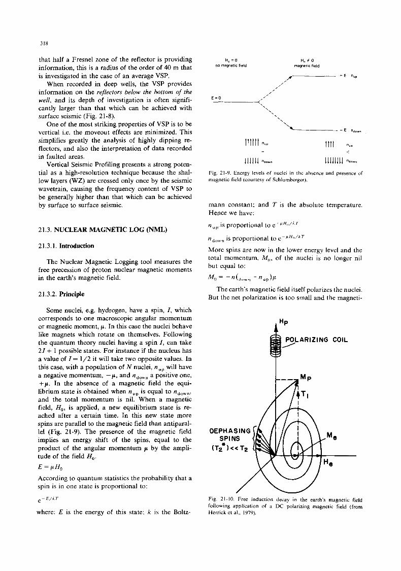
318
that half a Fresnel zone of the reflector is providing information, this is a radius of the order of 40 m that is investigated in the case of an average VSP.
When recorded in deep wells, the VSP provides information on the reflectors below the bottom of the well, and its depth of investigation is often signifi- cantly larger than that which can be achieved with surface seismic (Fig. 21-8).
One of the most strikmg properties of VSP is to be vertical i.e. the moveout effects are minimized. This simplifies greatly the analysis of highly dipping re- flectors, and also the interpretation of data recorded in faulted areas.
Vertical Seismic Profiling presents a strong poten- tial as a high-resolution technique because the shal- low layers (WZ) are crossed only once by the seismic wavetrain, causing the frequency content of VSP to be generally higher than that which can be achieved by surface to surface seismic.
21.3. NUCLEAR MAGNETIC LOG (NML)
21.3.1. Introduction
The Nuclear Magnetic Logging tool measures the free precession of ho ton nuclear magnetic moments in the earth's magnetic field.
21.3.2. Principle
Some nuclei, e.g. hydrogen, have a spin, I , which corresponds to one macroscopic angular momentum or magnetic moment, p . In this case the nuclei behave like magnets which rotate on themselves. Following the quantum theory nuclei having a spin I , can take 2 1 + 1 possible states. For instance if the nucleus has a value of 1 = 1/2 it will take two opposite values. In this case, with a population of N nuclei, nup will have a negative momentum, - p , and ndown a positive one, + p . In the absence of a magnetic field the equi- librium state is obtained when nup is equal to ndown, and the total momentum is nil. When a magnetic field, H,, is applied, a new equilibrium state is re- ached after a certain time. In t h s new state more spins are parallel to the magnetic field than antiparal- lel (Fig. 21-9). The presence of the magnetic field implies an energy shift of the spins, equal to the product of the angular momentum p by the ampli- tude of the field H,.
E = p H ,
According to quantum statistics the probability that a spin is in one state is proportional to:
- E / h T
where: E is the energy of this state; k is the Boltz-
H,=O no magfietic field
t t t t t t nuP
H, Z 0 magnetic field
+ E nyp f , ,
Fig. 21-9. Energy levels of nuclei in the absence and presence of magnetic field (courtesy of Schlumberger).
mann constant; and T is the absolute temperature. Hence we have:
n up. is proportional to e + s' '~~/ '
n,,,," is proportional to eppH11/'7
More spins are now in the lower energy level and the total momentum, M,,, of the nuclei is no longer nil but equal to: 4
Mo = - n L n - n"&
The earth's magnetic fieId itself polarizes the nuclei. But the net polarization is too small and the magneti-
AHP
OEPH A S IN G
/ w Fig. 21-10. Free induction decay in the earth's magnetic field following application of a DC polarizing magnetic field (from Herrick et al.. 1979).
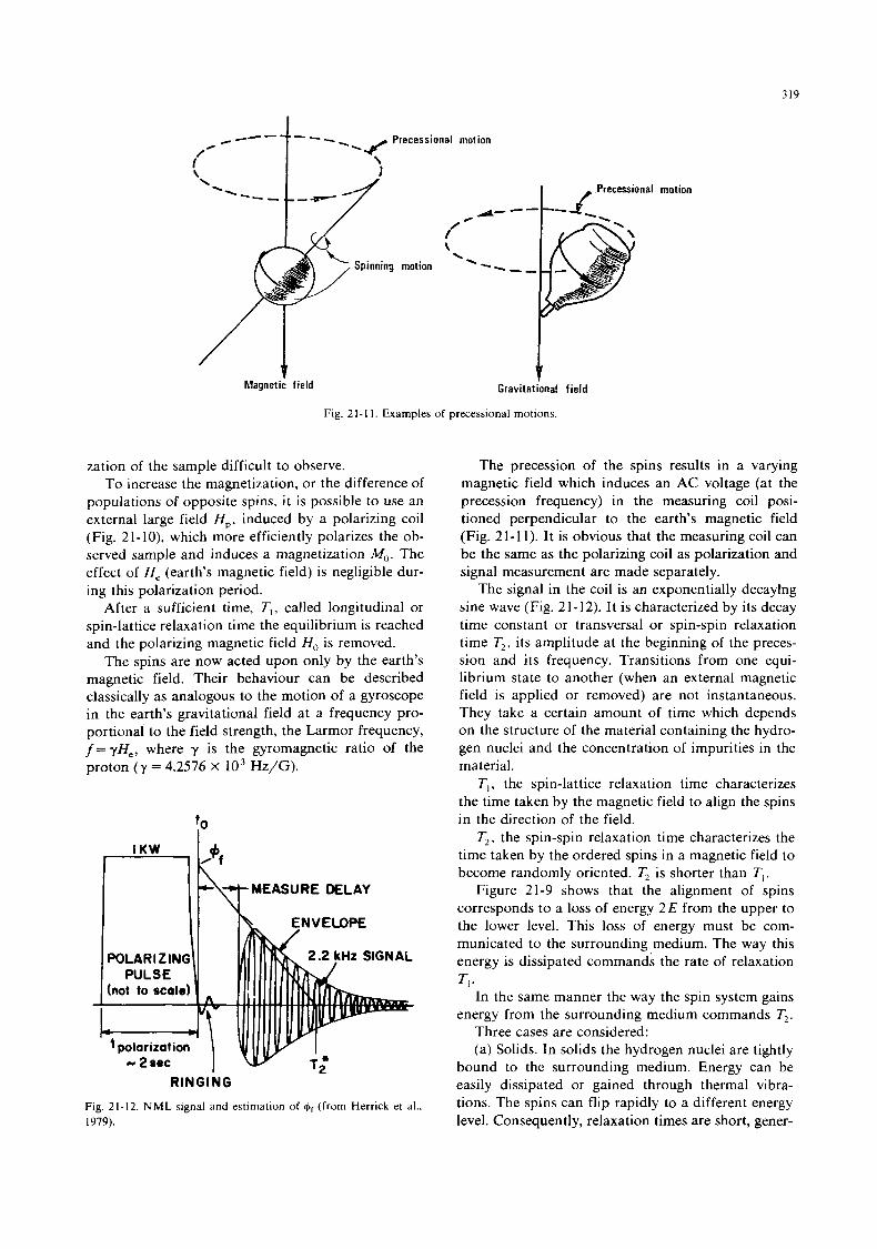
319
, '> Spinning motion - - ---
I
Gravitat iona! field Magneti; field
Fig. 2 1 - 1 1. Examples of precessional motions.
zation of the sample difficult to observe. To increase the magnetization, or the difference of
populations of opposite spins, i t is possible to use an external large field H,,, induced by a polarizing coil (Fig. 21- lo), which more efficiently polarizes the ob- served sample and induces a magnetization Mc,. The effect of He (earth's magnetic field) is negligible dur- ing this polarization period.
After a sufficient time, TI, called longitudinal or spin-lattice relaxation time the equilibrium is reached and the polarizing magnetic field H , is removed.
The spins are now acted upon only by the earth's magnetic field. Their behaviour can be described classically as analogous to the motion of a gyroscope in the earth's gravitational field at a frequency pro- portional to the field strength, the Larmor frequency, f = yH,, where y is the gyromagnetic ratio of the proton ( y = 4.2576 x lo3 Hz/G).
POLAR I Z I NG PULSE
t polarization - 2sec RINGING
Fig. 21-12. N M L signal and estimation of Gr (from Herrick et al.. 1979).
motion
The precession of the spins results in a varying magnetic field which induces an AC voltage (at the precession frequency) in the measuring coil posi- tioned perpendicular to the earth's magnetic field (Fig. 21-1 1). It is obvious that the measuring coil can be the same as the polarizing coil as polarization and signal measurement are made separately.
The signal in the coil is an exponentially decaylng sine wave (Fig. 21-12). It is characterized by its decay time constant or transversal or spin-spin relaxation time T,, its amplitude at the beginning of the preces- sion and its frequency, Transitions from one equi- librium state to another (when an external magnetic field is applied or removed) are not instantaneous. They take a certain amount of time which depends on the structure of the material containing the hydro- gen nuclei and the concentration of impurities in the material.
T, , the spin-lattice relaxation time characterizes the time taken by the magnetic field to align the spins in the direction of the field.
T,, the spin-spin relaxation time characterizes the time taken by the ordered spins in a magnetic field to become randomly oriented.
Figure 21-9 shows that the alignment of spins corresponds to a loss of energy 2 E from the upper to the lower level. This loss of energy must be com- municated to the surrounding medium. The way this energy is dissipated commands the rate of relaxation
In the same manner the way the spin system gains energy from the surrounding medium commands T,.
Three cases are considered: (a) Solids. In solids the hydrogen nuclei are tightly
bound to the surrounding medium. Energy can be easily dissipated or gained through thermal vibra- tions. The spins can flip rapidly to a different energy level. Consequently, relaxation times are short, gener-
is shorter than T, .
TI .
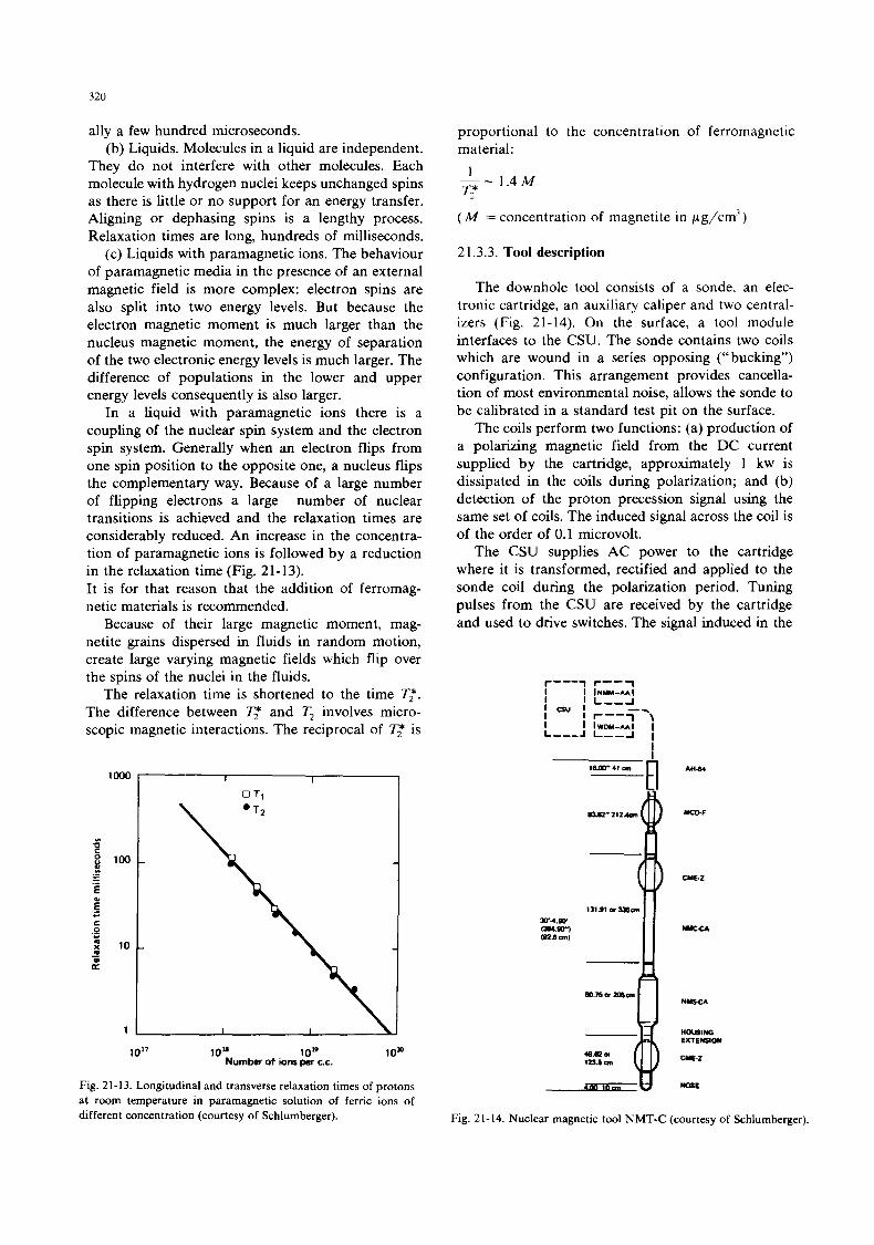
320
ally a few hundred microseconds. (b) Liquids. Molecules in a liquid are independent.
They do not interfere with other molecules. Each molecule with hydrogen nuclei keeps unchanged spins as there is little or no support for an energy transfer. Aligning or dephasing spins is a lengthy process. Relaxation times are long, hundreds of milliseconds.
(c) Liquids with paramagnetic ions. The behaviour of paramagnetic media in the presence of an external magnetic field is more complex: electron spins are also split into two energy levels. But because the electron magnetic moment is much larger than the nucleus magnetic moment, the energy of separation of the two electronic energy levels is much larger. The difference of populations in the lower and upper energy levels consequently is also larger.
In a liquid with paramagnetic ions there is a coupling of the nuclear spin system and the electron spin system. Generally when an electron flips from one spin position to the opposite one, a nucleus flips the complementary way. Because of a large number of flipping electrons a large number of nuclear transitions is achieved and the relaxation times are considerably reduced. An increase in the concentra- tion of paramagnetic ions is followed by a reduction in the relaxation time (Fig. 2 1- 13). It is for that reason that the addition of ferromag- netic materials is recommended.
Because of their large magnetic moment, mag- netite grains dispersed in fluids in random motion, create large varying magnetic fields which flip over the spins of the nuclei in the fluids.
The relaxation time is shortened to the time T:. The difference between T: and T2 involves micro- scopic magnetic interactions. The reciprocal of T: is
100
10
1
10" 10' 10" 1 om Number of ions per C.C.
Fig. 21-13. Longitudinal and transverse relaxation times of protons at room temperature in paramagnetic solution of ferric ions of different concentration (courtesy of Schlumberger).
proportional to the concentration of ferromagnetic material:
1 -- 1.4 M T,*
( M = concentration of magnetite in pg/cm3)
2 1.3.3. Tool description
The downhole tool consists of a sonde, an elec- tronic cartridge, an auxiliary caliper and two central- izers (Fig. 21-14). On the surface, a tool module interfaces to the CSU. The sonde contains two coils which are wound in a series opposing ("bucking") configuration. This arrangement provides cancella- tion of most environmental noise, allows the sonde to be calibrated in a standard test pit on the surface.
The coils perform two functions: (a) production of a polarizing magnetic field from the DC current supplied by the cartridge, approximately 1 kw is dissipated in the coils during polarization; and (b) detection of the proton precession signal using the same set of coils. The induced signal across the coil is of the order of 0.1 microvolt.
The CSU supplies AC power to the cartridge where it is transformed, rectified and applied to the sonde coil during the polarization period. Tuning pulses from the CSU are received by the cartridge and used to drive switches. The signal induced in the
WE.2
NYCCA
NYZCA
NOSE
Fig. 2 1-14. Nuclear magnetic tool NMT-C (courtesy of Schlumberger).
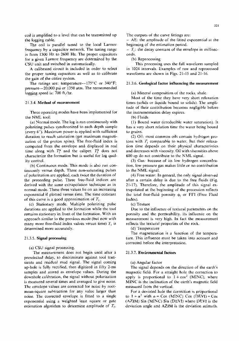
32 1
coil is amplified to a level that can be transmitted up the logging cable.
The coil is parallel tuned to the local Larmor frequency by a capacitor network. The tuning range is from 1300 Hz to 2600 Hz. The proper capacitors for a given Larmor frequency are determined by the CSU unit and switched in automatically.
A calibrated circuit is included in order to select the proper tuning capacitors as well as to calibrate the gain of the entire system.
The ratings are: temperature- 175°C or 340°F; pressure-20,000 psi or 1350 atm. The recommended logging speed is: 700 ft/hr.
2 1.3.4. Method of measurement
Three operating modes have been implemented for the NML tool:
(a) Normal mode. The log is run continuously with polarizing pulses synchronized to each depth sample (every 6”). Maximum power is applied with sufficient duration to reach saturation (get maximum magneti- zation of the proton spins). The free-fluid index is computed from the envelope and displayed in real time along with T; and the caliper. T: does not characterize the formation but is useful for log qual- ity control.
(b) Continuous mode. This mode is also run con- tinuously versus depth. Three non-saturating pulses of polarization are applied, each twice the duration of the preceeding pulse. Three free-fluid indices are derived with the same extrapolation technique as in normal mode. These three values lie on an increasing exponential if plotted versus time. The time constant of this curve is a good approximation of T , .
(c) Stationary mode. Multiple polarizing pulse durations are applied to the formation while the tool remains stationary in front of the formation. With an approach similar to the previous mode (but now with many more free-fluid index values versus time) Ti is determined more accurately.
2 1.3.5. Signal processing
(a) CSU signal processing. The measurement does not begin until after a
preselected delay, to discriminate against tool tran- sients and residual mud signal. The signal coming up-hole i s fully rectified, then digitized in fifty 2-ms samples and stored as envelope values. During the downhole calibration, the signal without polarization is measured several times and averaged to give noise. The envelope values are corrected for noise by root- mean-square subtraction for any value larger than noise. The corrected envelope is fitted to a single exponential using a weighted least square or gate estimation algorithm to determine amplitude of T,.
The outputs of the curve fittings are: - AE: the amplitude of the fitted exponential at the beginning of the estimation period. - T,: the decay constant of the envelope in millisec- onds.
(b) Reprocessing This processing uses the full waveform sampled
in 1024 intervals. Examples of raw and reprocessed waveforms are shown in Figs. 2 1 - 15 and 2 1 - 16.
2 1.3.6. Geological factor influencing the measurement
(a) Mineral composition of the rocks, shale. Most of the time they have very short relaxation
times (solids or liquids bound to solids). The ampli- tude of their contribution becomes negligible before the instrumentation delay expires.
(b) Fluids (1) Bound water (irreducible water saturation). I t
has a very short relation time the water being bound to grains.
( 2 ) Oil: most common oils contain hydrogen pro- tons with Ti comparable to water. But their relaxa- tion time depends on their physical characteristics and decreases with viscosity. Oil with viscosities above 600 cp do not contribute to the NML signal.
(3) Gas: because of its low hydrogen concentra- tion, low pressure gas makes little or no contribution to the NML signal.
(4) Free water: In general, the only signal observed after a certain delay is due to the free fluids (Fig. 2 1 - 17). Therefore, the amplitude of this signal ex- trapolated at the beginning of the precession reflects the total free-fluid porosity Gf or FFI (Free Fluid Index).
(c) Texture Due to the influence of textural parameters on the
porosity and the permeability, its influence on the measurement is very high. In fact the measurement reflects the textural properties of the rock.
(d) Temperature The magnetization is a function of the tempera-
ture. This influence must be taken into account and corrected before the interpretation.
21.3.7. Environmental factors
(a) Angular factor The signal depends on the direction of the earth’s
magnetic field. For a straight hole the correction to apply is proportional to 1 + cos’ (MINC), where MINC is the inclination of the earth’s magnetic field measured from the vertical.
For a deviated hole the correction is proportional to 1 + a‘ with a = Cos (MINC) Cos (DEVI) + Cos (AZIM) Sin (MINC) Sin (DEVI) where DEVI is the deviation angle and AZIM is the deviation azimuth.
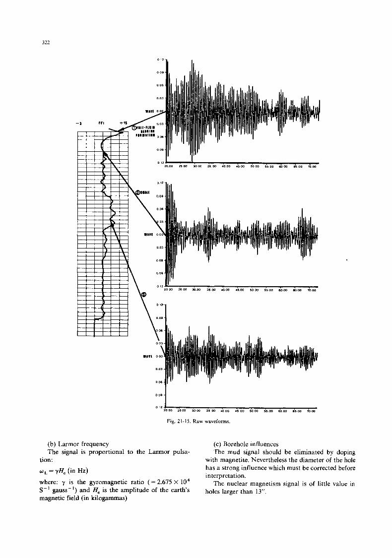
322
0 1 2 * I
(b) Larmor frequency
2000 2 5 0 0 mom 3500 1000 4500 5000 5 5 0 0 0000 moo moo o ’ 2 1 ‘
0 12 2000 2500 3000 35 W 1000 45 00 50 00 55 00 $000 (1500 7b 00
Fig. 21-15. Raw waveforms.
(c ) Borehole influences The signal is proportional to the Larmor pulsa- The mud signal should be eliminated by doping
with magnetite. Nevertheless the diameter of the hole has a strong influence which must be corrected before interpretation.
The nuclear magnetism signal is of little value in holes larger than 13”.
tion: w L = yH, (in Hz)
where: y is the gyromagnetic ratio (= 2.675 X lo4 S- ’ gauss-’) and He is the amplitude of the earth‘s magnetic field (in kilogammas)
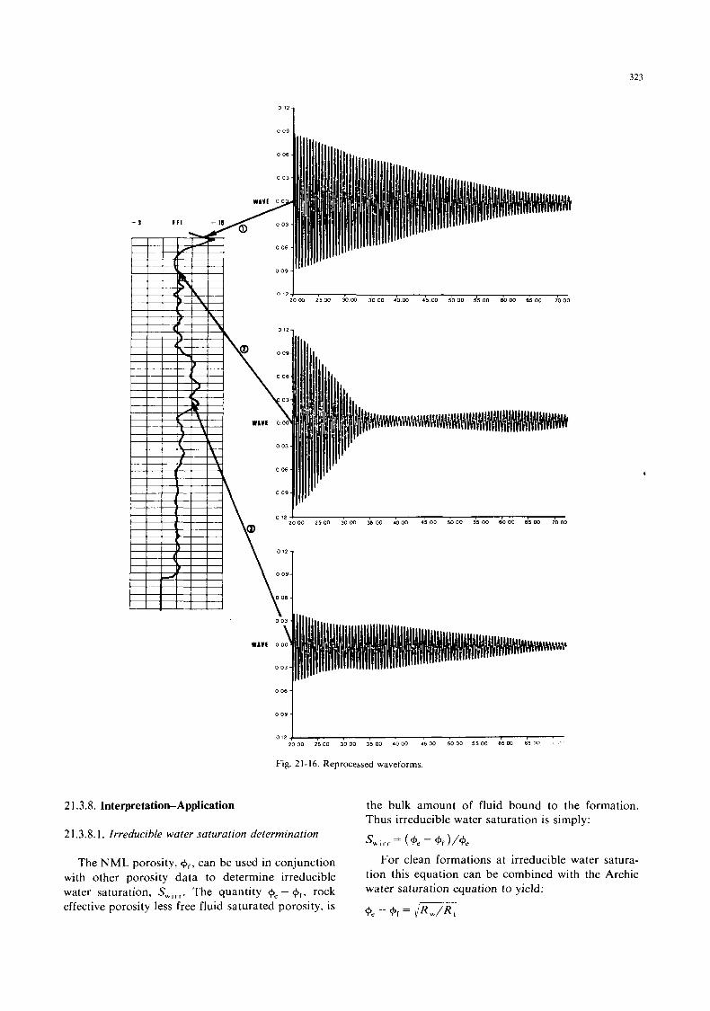
323
0 12 20 00 2500 30 00 35 00 4 0 00 45 00 50 00 5 5 00 65 W 65 @I, I '
Fig. 21-16. Reprocessed waveforms.
2 1.3.8. Interpretation-Application
2 1.3.8.1. Irreducible water saturation determination
the bulk amount of fluid bound to the formation. Thus irreducible water saturation is simply:
S w , r r = ( + e - + f ) / + e
The NML porosity, +f, can be used in conjunction with other porosity data to determine irreducible water saturation, S,,,,. The quantity +e - +f, rock effective porosity less free fluid saturated porosity, is
For clean formations at irreducible water satura- tion this equation can be combined with the Archie water saturation equation to Yield:
+e - +[ = / R J R , I
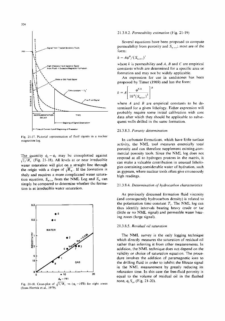
324
2 1.3.8.2. Permeability estimation (Fig. 2 1 - 19)
\ \. ,Shale or Silt Fluid Signal
‘\ ,Time constant = T2*
TIME L Begining of Signal Observation
INSTRUMENTATION DELAY i Time of Current Cutoff Beginning of Precession
Fig. 21-17. Pictorial representation of fluid signals in a nuclear magnetism log.
The quantity Ge - (pf may be crossplotted against J1/R, (Fig. 21-18). All levels at or near irreducible water saturation will plot on a straight line through the origin with a slope of 6. If the formation is shaly and requires a more complicated water satura- tion equation, Swirr from the NML Log and S, can simply be compared to determine whether the forma- tion is at irreducible water saturation.
0.3 , a5
0.5
I WATER I a2 i”/l ,,OP
d
0 10 20
& - FFI
Fig. 21-18. Cross-plot of \/1/R. vs ( & -FFI) for eight zones (from Hemck et al., 1979).
Several equations have been proposed to compute permeability from porosity and S, , , , ; most are of the form:
k = AG’/( S w r r
where k is permeability and A , B and C are empirical constants which are determined for a specific area or formation and may not be widely applicable.
An expression for use in sandstones has been proposed by Timur (1969) and has the form:
where A and B are empirical constants to be de- termined for a given lithology. Either expression will probably require some initial calibration with core data after which they should be applicable to subse- quent wells drilled in the same formation.
2 1.3.8.3. Porosity determination
In carbonate formations, which have little surface activity, the NML tool measures essentially total porosity and can therefore supplement existing com- mercial porosity tools. Since the NML log does not respond at all to hydrogen protons in the matrix, it can make a valuable contribution in unusual litholo- gies containing considerable water of hydration, such as gypsum, where nuclear tools often give erroneously high readings.
2 1.3.8.4. Determination of hydrocarbon characteristics
As previously discussed formation fluid viscosity (and consequently hydrocarbon density) is related to the polarization time constant T,. The NML log can thus identify intervals bearing heavy crude or tar (little or no NML signal) and permeable water bear- ing zones (large signal).
21.3.8.5. Residual oil saturation
The NML survey is the only logging technique which directly measures the saturation of residual oil rather than inferring it from other measurements. In addition, the NML technique does not depend on the validity or choice of saturation equation. The proce- dure involves the addition of paramagnetic ions to the drilling fluid in order to inhibit the filtrate signal in the NML measurement by greatly reducing its relaxation time. In this case the free-fluid porosity is equal to the volume of residual oil in the flushed zone, Ge.SOr (Fig. 21-20).
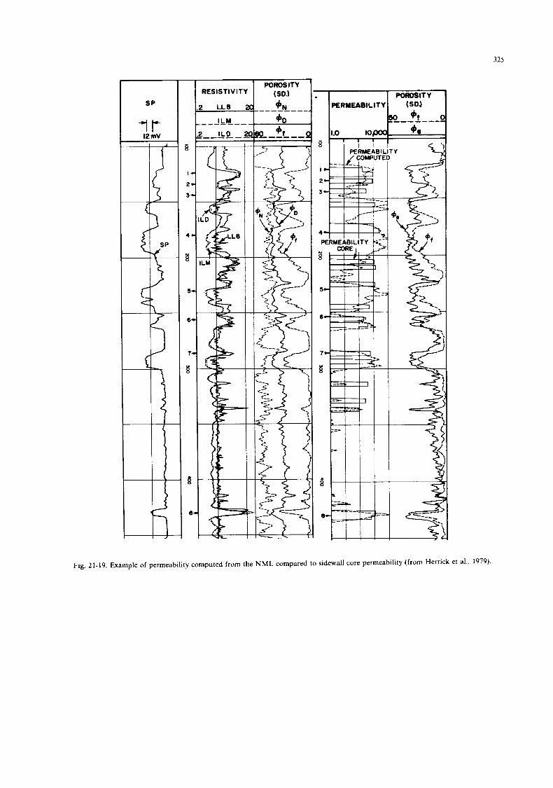
325
*tt-t- PERMEABILITY
==I 3; ---=-----
Fig. 21-19. Example of permeability computed from the NML compared to sidewall core permeability (from Herrick et al., 1979).
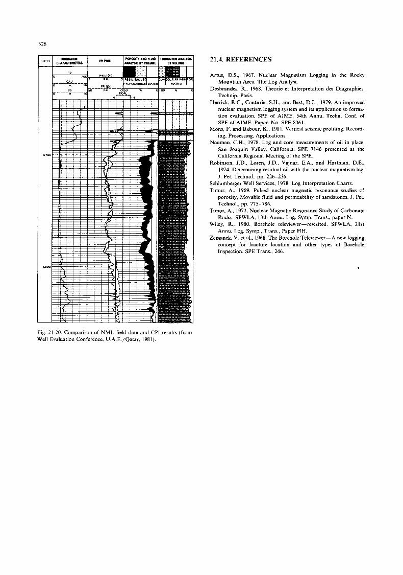
326
2 1.4. REFERENCES
Artus, D.S., 1967. Nuclear Magnetism Loggng in the Rocky Mountain Area. The Log Analyst.
Desbrandes, R., 1968. Theorie et Interpretation des Diagraphies. Technip, Paris.
Herrick, R.C., Couturie, S.H., and Best, D.L., 1979. An improved nuclear magnetism logging system and its application to forma- tion evaluation. SPE of AIME, 54th Annu. Techn. Conf. of SPE of AIME. Paper. No. SPE 8361.
Mons, F. and Babour, K., 1981. Vertical seismic profiling. Record- ing, Processing, Applications.
Neuman, C.H., 1978. Log and core measurements of oil in place, , San Joaquin Valley, California. SPE 7146 presented at the California Regional Meeting of the SPE.
Robinson, J.D., Loren, J.D., Vajnar, E.A., and Hartman, D.E., 1974. Determining residual oil with the nuclear magnetism log. J. Pet. Technol., pp. 226-236.
Schlumberger Well Services, 1978. Log Interpretation Charts. Timur, A,, 1969. Pulsed nuclear magnetic resonance studies of
porosity, Movable fluid and permeability of sandstones. J. Pet. Technol., pp. 775-786.
Timur, A,, 1972. Nuclear Magnetic Resonance Study of Carbonate Rocks. SPWLA, 13th Annu. Log. Symp. Trans., paper N.
Wiley, R., 1980. Borehole televiewer-revisited. SPWLA, 2lst Annu. Log. Symp., Trans., Paper HH.
Zemanek, V. et al., 1968. The Borehole Televiewer-A new logging concept for fracture location and other types of Borehole Inspection. SPE Trans., 246.
Fig. 21-20. Comparison of NML field data and CPI results (from Well Evaluation Conference, U.A.E./Qatar, 1981).
327
22. THE PLACE AND ROLE OF LOGS IN THE SEARCH FOR PETROLEUM
Let us suppose that i t was possible to core a well continuously to total depth. We could conclude that in this case there would be no real use in running logs, since the geologists, reservoir engineers and drilling engineers apparently have on hand all the samples necessary for their particular studies. How- ever, they still lack certain information:
(a) Data that are difficult or expensive to obtain (measurements of natural gamma-ray radiation, neu- tron hydrogen index, sonic transit time, bulk density, etc.).
(b) An analysis of a larger volume of formation than the core, especially when we consider that core measurements are themselves made on thin sections or plugs of material.
(c) The possibility of making a computer analysis of quantitative data as with logs.
(d) Information which is permanent. Everyone, therefore realizes that continuous coring
without running logs is not a reasonable economic way of evaluating a formation. In any case since there is almost always a risk of a less than 100 percent core recovery then there is also a risk of having gaps in the well information.
These are some of the reasons why the last 50 years has seen almost continuous research into tech- niques that attempt to cover deficiencies in core data. Logs make up the majority of these techniques. The number of types of logs and their reliability has increased and new interpretation methods have been developed simultaneously.
Logs, having become in some ways the geologist's eye-an eye that is imperfect and sometimes dis- torted but nevertheless not blind-and an instrument for the reservoir engineer, occupy a special place and play an important role in petroleum research by the economies that they bring and the amount of infor- mation they contain.
Desbrandes (1968) estimated that the cost of log- ging was 2% of the total drilling cost whereas the information that they supplied on the content of reservoirs was obtained at some one fifth of the cost of any other comparable method.
From a statistical study made by the drilling de- partment of the Elf-Aquitaine group on 43 wells operated by the group in 1973, it turns out that the cost of logging operations, measured by the total bills paid to service companies, was 5% of the drilling costs, leaving out the immobilisation time of the
necessary equipment (the rig) or production opera- tions. If this time is added, the total cost comes to about 10%.
The amount of money that is saved is more dif- ficult to determine but we can estimate that continu- ous coring would triple the drilling costs. In the same way, formation tests that are made without reliable information on their positioning in depth, or their necessity, raise costs very strongly.
All the same even if logging can be shown to be an economical and practical method of obtaining data we can always conceive of methods of reducing over- all logging costs. Several issues need to be considered before doing this:
(1) All geological or other information either comes from samples collected during drilling (cores, cut- tings, wireline cores) and testing (fluid samples) or from logs. While the cost of coring and testing is often less than 5% of the well cost and geologi'cal monitoring less than 2% it is evident that good qual- ity samples are rare and relatively expensive. If the logging program is limited we risk losing part of our only other source of information. This is a false economy since we risk losing information that is more valuable than the costs saved.
(2) The economy may show up in the long term to be disastrous. When a study of a basin or field is made the lack of information may lead to the non- identification of a potential well or zone.
(3) In recording logs we include information that may not be of immediate use but which may show up as useful later on.
(4) Reducing the frequency of logging may lead to the loss of information entirely as in the case where a well is lost before the next logging point is reached or where further drilling deteriorates the well conditions to the point where good quality logs are unobtainable (well caving in or deep invasion).
(5) Redundant information should not be eliminated since it acts as a control of the quality of the recording.
(6 ) Logs are obtained rapidly after the completion of drilling, are easily transported, easily compared and are a relatively indestructable form of informa- tion.
We have to then measure the economies made in terms of the actual information given by each log and the risk involved when this information is not availa- ble.
328
We can obtain an idea of the information given by each log by looking at Table 1-4 of this volume and the paragraphs on geological factors influencing mea- surements and applications.
Table 22-1 gives a more complete idea by looking at the information obtained from each log singly or in combination with others and by classifying them as more or less quantitative or qualitative.
We need to clearly establish the areas of applica- tion of logs. These and the corresponding interpreta- tion methods will be the subject of volume 2 which will cover the following subjects:
(a) Description of sedimentary series: ( 1) their mineral composition and lithology; ( 2 ) their texture; (3) their sedimentary structure (4) the petrophysical characteristics of the re-
(5) the nature of the reservoir fluids. servoirs;
(b) The formation of sedimentary series (sedimentology) attempting to reconstruct the depositional environment from:
(1) a facies type analysis; (2) analysis of sequences; (3) facies correlation.
(c) Transformation of sediments. The effects of diagenesis, their identification, compaction studies.
(d) The organisation of sedimentary series (stratig- raphy)
(1 ) study of their order and relative age; ( 2 ) the significance of ruptures (discontinui-
(3) stratigraphic correlation.
ural geology) (1) folds; (2) faults; (3) fractures.
plications.
synthesis.
ties);
(e) The deformation of sedimentary series (struct-
(f) Geophysical, geothermal and geochemical ap-
(g) Role and importance of logs in geological
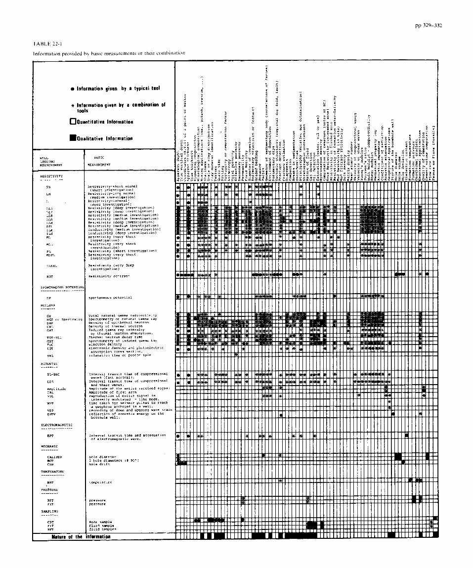

333
APPENDIX 1
TABLE Al-l
List of open hole logging tools and their symbol
OPEN HOLE LOGGING-Formation Evaluation Logs
Electrical Survey * Birdwell
Dresser Atlas GO International Schlumberger
Welex
Electric Log Single Point Resistivity Log Electrolog Electrical Log Electrical Survey Salt Dome Profiling (ULSEL *) Electric Log Drill Pipe Electric Log *
ES
EL EL ES ES-U LS
Induction Logs * (focused conductivity) Birdwell
Dresser Atlas
GO International
Schlumberger
Welex
Focused Resistivity L o g Birdwell Dresser Atlas
GO International Schlumberger
Welex
Induction Log Induction Electric Log Induction Electrolog Dual Induction Focused Log Induction Log Induction-Electrical Log Induction Log Induction-Electrical Survey ISF Induction Log Dual Induction-Laterolog Dual Induction-SFL Induction Electric Log/Long Lateral Dual Induction Guard
Guard Log * Laterolog * Dual Laterolog Guard Log * Laterolog * Dual Laterolog * Spherically Focused Log * Guard Log * Guard-FoRxo
Micro - resistivity Log (non -focused, Microlog * type) Birdwell Micro-Contact Caliper Dresser Atlas Minilog GO International Micro-Electrical Log Schlumberger Microlog Welex Contact Caliper Log
Micro - resistivity Log (focused, Microlaterolog * type) Dresser Atlas Micro-Laterolog
GO International Micro-Guard Schlumberger Microlaterolog
Proximity *-Minilog
Proximity *-Microlog Micro-SFL
Welex FoRxo-Caliper Log
Gamma - Ray Log * (natural gamma) Birdwell Gamma-Ray Log Dresser Atlas Gamma-Ray Log GO-International Gamma-Ray Log M c C u 11 o u gh Gamma-ray
1s I ES I EL DIFL IL IEL
I ES ISF DIL
IEL DIGL
GDS IL
GL L DLL SFL
EMC ML ML ML
MLL PML MGL MLL PLL
GR
This Page Intentionally Left Blank
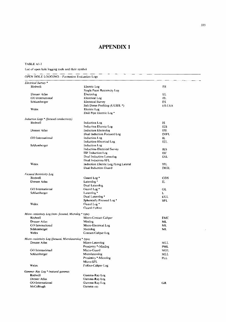
333
APPENDIX 1
TABLE Al-l
List of open hole logging tools and their symbol
OPEN HOLE LOGGING-Formation Evaluation Logs
Electrical Survey * Birdwell
Dresser Atlas GO International Schlumberger
Welex
Electric Log Single Point Resistivity Log Electrolog Electrical Log Electrical Survey Salt Dome Profiling (ULSEL *) Electric Log Drill Pipe Electric Log *
ES
EL EL ES ES-U LS
Induction Logs * (focused conductivity) Birdwell
Dresser Atlas
GO International
Schlumberger
Welex
Focused Resistivity L o g Birdwell Dresser Atlas
GO International Schlumberger
Welex
Induction Log Induction Electric Log Induction Electrolog Dual Induction Focused Log Induction Log Induction-Electrical Log Induction Log Induction-Electrical Survey ISF Induction Log Dual Induction-Laterolog Dual Induction-SFL Induction Electric Log/Long Lateral Dual Induction Guard
Guard Log * Laterolog * Dual Laterolog Guard Log * Laterolog * Dual Laterolog * Spherically Focused Log * Guard Log * Guard-FoRxo
Micro - resistivity Log (non -focused, Microlog * type) Birdwell Micro-Contact Caliper Dresser Atlas Minilog GO International Micro-Electrical Log Schlumberger Microlog Welex Contact Caliper Log
Micro - resistivity Log (focused, Microlaterolog * type) Dresser Atlas Micro-Laterolog
GO International Micro-Guard Schlumberger Microlaterolog
Proximity *-Minilog
Proximity *-Microlog Micro-SFL
Welex FoRxo-Caliper Log
Gamma - Ray Log * (natural gamma) Birdwell Gamma-Ray Log Dresser Atlas Gamma-Ray Log GO-International Gamma-Ray Log M c C u 11 o u gh Gamma-ray
1s I ES I EL DIFL IL IEL
I ES ISF DIL
IEL DIGL
GDS IL
GL L DLL SFL
EMC ML ML ML
MLL PML MGL MLL PLL
GR
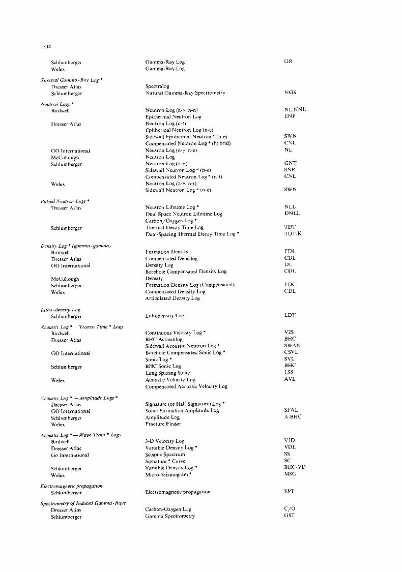
334
Schlumberger Welex
Spectral Gammo - Rqv Log * Dresser Atlas Schlumberger
Neutron Logs * Birdwell
Gamma-Ray Log Gamma-Ray Log
G R
Spectralog Natural Gamma-Ray Spectrometry NGS
NL.NNL EN P
Neutron Log (n-y, n-n) Epithermal Neutron Log Neutron Log (n-t) Epithermal Neutron Log (n-e) Sidewall Epithermal Neutron * (n-e) Compensated Neutron Log * (hybrid) Neutron Log (n-y, n-e) Neutron Log Neutron Log (n-y) Sidewall Neutron Log * (n-e) Compensated Neutron Log * (n-t) Neutron Log (n-y. n-t) Sidewall Neutron Log * (n-e)
Dresser Atlas
SWN CNL NL G O International
McCullough Schlumberger G N T
SN P CNL
Welex SWN
Pulsed Neutron Logs * Dresser Atlas Neutron Lifetime Log *
Dual Space Neutron Lifetime Log Carbon/Oxygen Log * Thermal Decay Time Log Dual-Spacing Thermal Decay Time Log *
NLL DNLL
Schlumberger T D T TDT-K
Density Log * (gamma -gamma) Birdwell Dresser Atlas G O International
Formation Density Compensated Densilog Density Log Borehole Compensated Density Log Density Formation Density Log (Compensated) Compensated Density Log Articulated Density Log
FDL CDL DL CDL
. McCullough Schlumberger Welex
FDC CDL
Litho -densrty Log Schlumberger
Acoustic Lag *-Transit Time * Logs Birdwell Dresser Atlas
LDT Lithodensity Log
Continuous Velocity Log * BHC Acoustilog Sidewall Acoustic Neutron Log * Borehole Compensated Sonic Log * Sonic Log * BHC Sonic Log Long Spacing Sonic Acoustic Velocity Log Compensated Acoustic Velocity Log
v 2 s BHC SWAN CSVL SVL BHC LSS AVL
G O International
Schlumberger
Welex
Acoustic Log a - Amplitude Logs * Dresser Atlas G O International Schlumberger Welex
Acoustic Log * - Wave Train * Logs Birdwell Dresser Atlas Go International
Signature (or Half Signature) Log * Sonic Formation Amplitude Log Amplitude Log Fracture Finder
SFAL A-BHC
3-D Velocity Log Variable Density Log * Seismic Spectrum Signature * Curve Variable Density Log * Micro-Seismogram *
V3D VDL ss sc BHC-VD MSG
Schlumberger Welex
Electromagnetic propagation Schlumberger
Spectrometry of Induced Gamma - Rays Dresser Atlas Schlumberger
Electromagnetic propagation EPT
C/O GST
Carbon-Oxygen Log Gamma Spectrometry

335
OPEN HOLE LOGGING-Special Purpose Logs and Services
Beta Log . . . . . . . . . . . . . . . . . . . . . . . . . . . . . . . . . . . . . . . . . . . . . . . . . .
Birdwell Beta Log BL
Borehole Camera Birdwell Borehole Camera * BC
Borehole Gravimeter * Gravilog Esso Vibrating String
Borehole Televiewer a
Birdwell Schlumberger Amoco Sandia
svs TVT
Seisviewer Borehole Televiewer (not avail. 1975) Borehole Televiewer Acoustic borehole Televiewer
Caliper Log * Birdwell Caliper Logging
Seiscaliper (sonar caliper *) Caliper Caliper Log Caliper Caliper
CA3, CA6, CAL csc
Dresser Atlas GO International Schlumberger Welex
CL CAL
Computed Analysis Logs * Birdwell COM-PRO LOGS
Elastic-Properties Log Dresser Atlas Schlumberger
EPILOG SYSTEMS SYNERGETIC LOG SYSTEMS (SARABAND, CORIBAND, GLOBAL, VOLAN) Mechanical Properties Log CAL SYSTEMS Welex
Core Slicer * Dresser Atlas Schlumberger
Tricore Diamond Core Slicer (not avail.) DCS
Dipmeter * Dresser Atlas FDIP
HRDIP Focused 3-Arm Diplog Hi Resolution 4-Arm Diplog Dipmeter Log 4-Arm High Resolution Digital Dipmeter Sedimentary Dipmeter Dip Log
GO International Schlumberger HDT-D
SHDT Welex
Directional Surveys * Birdwell Dresser Atlas GO International Schlumberger Welex
Continuous Directional Inclinometer Log Directional Survey Continuous Directional Survey
CDI
CDS CDR Continuous Directional Survey
Drift Log
Formation Tester * Dresser Atlas GO International Schlumberger
Formation Tester Formation Tester Formation Tester Formation Interval Tester Multiple Fluid Sampler Repeat Formation Tester Formation Tester Jet-Vac Tester
FT FT FT FIT MFS RFT
Welex
Nuclear Magnetism Lag * Dresser Atlas Nuclear Magnetism Log
(not avail. 1975) Nuclear Magnetism Log
NML NML Schlumberger
Sidewall Sample Taker * (percussion) Birdwell Dresser Atlas GO International Schlumberger Welex
SWD Core Gun Corgun Sidewall Coring Sidewall Coring Sidewall Coring
swc CST

336
Temperature Logs * Birdwell
Dresser Atlas
GO International
Schlumberger Welex
Well Seismic Schlumberger
Temperature Log Differential Temperature Log * Temperature Log Differential Temperature Log * Temperature Log Differential Temperature Log * High Resolution Thermometer Precision Temperature Log
Well Seismic Survey Vertical Seismic Profile
TL T L D
TL DTL HRT
WST VSP
.
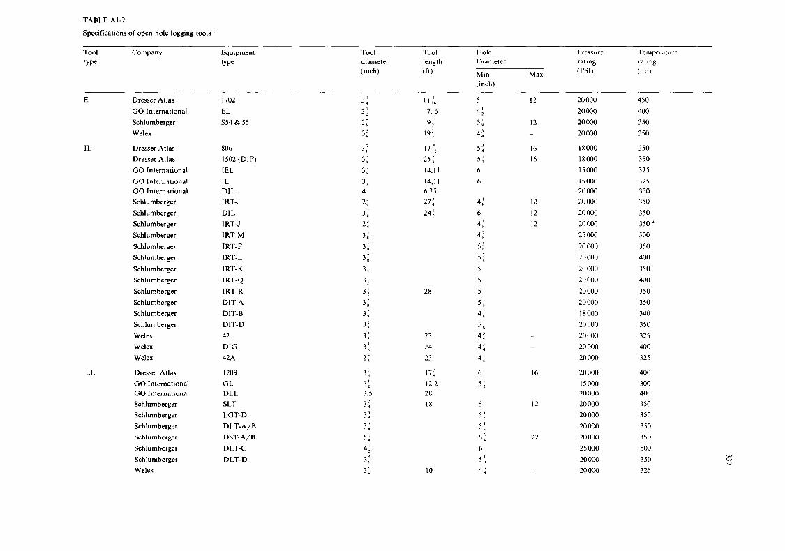
TABLE A 1-2
Specifications of open hole logging tools '
Tool Company type
Temperature Equipment Tool Tool Hole Pressure
type diameter length Diameter rating rating
(inch) ( f t ) Min Max ( O F ) (PSI)
(inch)
E Dresser Atlas GO International Schlumberger Welex
IL Dresser Atlas Dresser Atlas GO International GO International GO International Schlumberger Schlumberger Schlumberger Schlumberger Schlumberger Schlumberger Schlumberger Schlumberger Schlumberger Schlumberger Schlumberger Schlumberger Welex Welex Welex
Dresser Atlas GO International GO International Schlumberger Schlumberger Schlumberger Schlumberger Schlumberger Schlumberger Welex
LL
1702 3: 11 1: 5
EL s54 & 55
806 1502 (DIF) IEL IL DIL I RT- J DIL IRT-J IRT-M IRT-F IRT-L I RT- K
IRT-Q IRT-R DIT-A DIT-B DIT-D 42 DIG 42A
1209 GL DLL SLT LGT-D DLT-A/B DST-A/B DLT-C DLT-D
3: 3: 3:
3: 3;
3: 3:
2:
3: 2:
3: 3:
3: 3: 3;
3: 3: 3:
3: 3: 3: 2:
3: 3:
3: 3;
3: 5: 4;
3: 3:
4
3.5
7, 6
19;
17 25 2, 14,l I 14,Il 6.25 27 24 :
9:
28
23 24 23
17:
12,2 28 18
10
4: 5: 4;
5: 5: 6 6
4:
4: 4: 5: 5:
6
5
5 5
5 ;
4: 5: 4; 4:
4:
5 :
5 :
5 :
6
6
6; 6
5: 4:
12
22
12 20 000 20 000
12 20 000 - 20 000
16 18000 16 18 000
15 000 15000 20 000
12 20 000 12 20 000 12 20 000
25 000 20 000 20 000 20000 20 000 20 000 20 000 1 8 000 20 000 20 000 20 000 20 000
20 000 15 000 20 000 20 000 20 000 20 000 20 000 25 000 20 000 20 000
450 400 350 350
350 350 325 325 350 350 350 350 500 350 400 350 400 350 350 340 350 325 400 325
400 300 400 350 350 350 350 500 350 325
W W 4
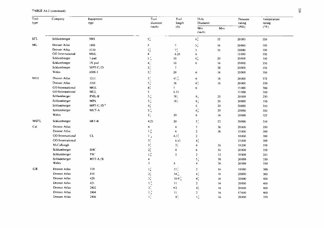
TABLE AI-2 (continued)
Tool Company Equipment Tool Tool Hole Pressure Temperature type type diameter length Diameter rating rating
(inch) ( f t ) Min Max (PSI) ( O F )
(inch)
W W M
SFL Schlumberger
M L Dresser Atlas Dresser Atlas G O International Schlumberger Schlumberger Schlumberger Welex
MLL Dresser Atlas Dresser Atlas G O International G O International Schlumberger Schlumberger Schlumberger Schlumberger Welex
MSFL Schlumberger
Cal Dresser Atlas Dresser Atlas G O International G O International McCullough Schlumberger Schlumberger Schlumberger Welex
G R Dresser Atlas Dresser Atlas Dresser Atlas Dresser Atlas Dresser Atlas Dresser Atlas Dresser Atlas
SRS
1 I06 11 10 MEL 1 pad 1X pad MPT-C/D 6000-3
1211
3101 MGL MLL PML-B MPS MPT-C/D MLT-A
SRT-B
CL
SHC TIC BGT-A/B
310 414 420 42 1
2402 2404 2406
7
7: 6,25
10
10
7 20
11 :2 16
? 6.33
18; 18;
20
20
4 6
6.3 6.11
3; 8
5
6:
5:
6:
5 6
6
6
6
6: 6
6 :
6 :
6:
5 ;
6
6
5 2 2
4: 4 6 2
5: 4
2
4;
4:
4;
1:
2
2
22
16 16
20 16 20 16
16 16
20 20 20 20 16
22
36 36
36 16 12 30 36
16
16 16 16 16 16 16
20 000
20 000 20 000 15000 20 000 20 000 20 000 20 000
20 000 20 000 15000 15 000 20 000 20 000 20 000 20 000 20 000
20 000
20 000 15 000 10 000 15 000 18 200 20 000 10 000 20 000 20 000
1 8 000 20 000 20 OOO
20 000 20 000 17 000 20 000
350
350 350 350 350 350 350 350
375 350 300 350 250 350 350 350 325
350
350 300 300 300 350 350 285 350 350
300 300 400 400 400 400
350
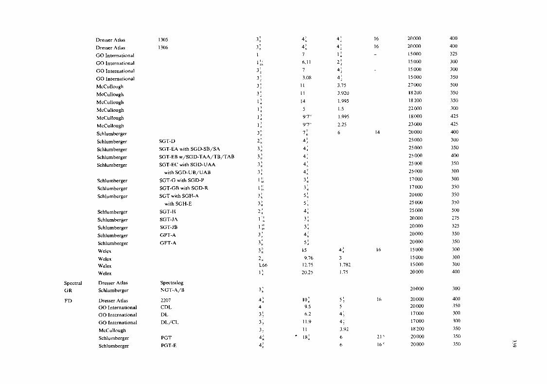
Dresser Atlas Dresser Atlas GO International GO International GO International GO International McCullough McCullough McCullough McCullough McCullough McCullough Schlumberger Schlumberger Schlumberger Schlumberger Schlumberger
Schlumberger Schlurnberger Schlurnberger
Schlumberger Schlumberger Schlumberger Schlumberger Schlumberger Welex Welex Welex Welex
Spectral Dresser Atlas GR Schlumberger
FD Dresser Atlas GO International GO International GO International McCullough Schlurnberger Schlurnberger
1305 1306
SGT-D SGT-EA with SGD-SB/SA SGT-EB w/SGD-TAA/TB/TAB SGT-EC with SGD-UAA
with SGD-UB/UAB SGT-G with SGD-P SGT-GB with SGD-R SGT with SGH-A
with SGH-E SGT-H SGT-JA SGT-JB GPT-A GFT-A
Spectralog NGT-A/B
2207 CDL DL DL/CL
PGT PGT-E
3;
4:
3;
3;
3;
4: 4:
4
4: 4: 7 6.1 1
7 3.08
1 1
1 1
14 5 9'7" 9'7"
7 :
4:
4: 4: 4: 4:
3:
3: 5 ;
5: 4: 3: 3: 4: 5:
15
9.76 12.75 20.25
10: 9.5 6.2
11.9 1 1
* 18:
4: 4:
1:
2: 4; 4; 3.75 3.920 1.995 1.5 1.995 2.25 6 14
16 20 000 16 20 000 - 15 000 ~ 15 000 - 15 000
15 000 27 000 18 200 18 200 22 000 18 000 23 000 20 000 25 000 25 000 25 000 25 000 25 000 I7 000 17 000 20 000 25 000 25 000 20 000 20 000 20 000 20 000 15 000 15 000 15 000 20 000
4: 16 3 I ,782 1.75
5 ;
4 ;
4 ;
5
3.92 6 6
16
21 16'
20 000
20 000 20 000 17 000 I7 000 I8 200 20 000 20 000
400 400 325 300 300 350 500 350 350 300 425 425 400 300 350 400 350 300 300 350 350 350 500 275 325 350 350 300 300 300 400
300
400 350 300 300 350 350 350
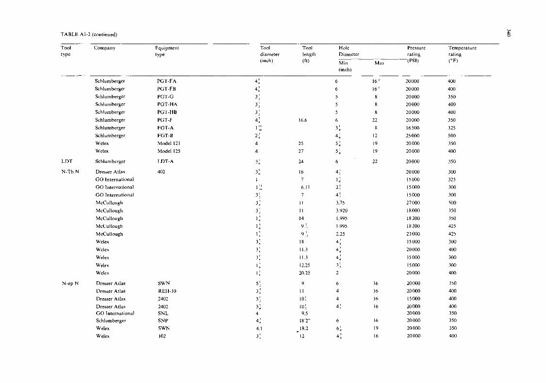
TABLE AI-2 (continued)
Tool Company Equipment Tool Tool Hole Pressure type type diameter length rating rating Diameter
Temperature
(inch) ( f t ) Min Max (PSI) ( O F ) (inch)
W P 0
Schlumberger Schlumberger Schlumberger Schlumberger Schlumberger Schlumberger Schlumberger Schlumberger Welex Welex
LDT Schlumberger
N-Th N Dresser Atlas G O International G O International G O International McCullough McCullough McCullough McCullough McCullough Welex Welex Welex Welex Welex
N-ep N Dresser Atlas Dresser Atlas Dresser Atlas Dresser Atlas G O International Schlumberger Welex Welex
PGT-FA PGT-FB PGT-G PGT-HA PGT- H B PGT-J FGT-A FGT-B Model 12 1
Model 125
LDT-A
402
SWN REH-I0 2402 2402 SN L SN P SWN 102
4; 4; 3;
3:
3; 4;
1 I: 2; 4 4
3:
3;
1
1 3;
3: 3;
1:
1:
1:
3:
3: 3;
1:
1:
5;
3: 3;
3:
4:
3:
4
4.1
16.6
25 21
24
16
7 6.11
/
1 1
I I 14
9 :z 9 ,?
18
11.3 11.3 12.25 20.25
9 1 1
10;
lo; 9.5
18'2'' 18.2 12
6
6
5 5 5 6
3: 4: 5: 5:
4; 1: 2; 4;
6
3.15 3.920 1.995 1.995 2.25
4:
4: 4: 3; 2
6
4 4 4;
6
6:
4:
16'
16
8 8
8
22 8
12 19 19
22
16
16
16
16
16
19 16
20 000 20 000 20 000 20 000 20 000 20 000 16500 25 000 20 000 20 000
20 000
20 000 15 000 15000 I5 000 21 000 18 000 18 200 18 200 23 000 15 000 20 000 15 000 15000 20 000
20 000 20 000
15000
20 000 20 000 20 000 20 000 20 000
400 400 350 400 400 350 325 500 350 400
350
300 325 300 300 500 350 350 425 425 300 400 300 300 400
350 400 400 400 350 350 350 400
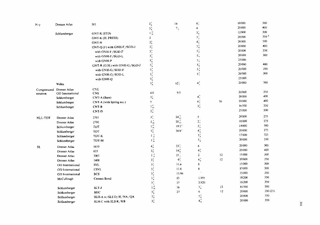
Dresser Atlas
Schlumberger
Welex
Compensated Dresser Atlas neutron GO International
Schlumberger Schlumberger Schlumberger
NLL-TDT Dresser Atlas Dresser Atlas Schlumberger Schlumberger Schlumberger Schlumberger
SL Dresser Atlas Dresser Atlas Dresser Atlas Dresser Atlas GO International GO International GO International McCullough
Schlumberger Schlumberger Schlumberger Schlumberger
30 1
GNT-K (STD) GNT-K (H. PRESS) GNT-N GNT-Q (F) with GNH-F/SGD-J
with GNH-F/SGD-F with GNH-F/SGD-L with GNH-P
GNT-R (G.H.) with GNH-G/SGD-J with GNH-G/SGD-F with GNH-G/SGD-L with GNH-Q
CNL CNS CNT-A (Bare) CNT-A (with Spring ecc.) CNT-B CNT-D
270 1
2702 TDT TDT TDT-K TDT-M
1610 623 3001 1408 SVL CSVL BCS Cement Bond
SLT-J BHC SLH-A w/SLS D/H/NA/QA SLH-C with SLS-K/KB
2: 3; 1 ;: 2: 3: 3: 3:
3: 3: 3: 3: 3: 3:
2
14
7:
12:
9.5
23 \ 14: 21;
9: 11.6 11.6 15.96 15 17 16 27
4;
3: 3: 4:
5: 5: 5 :
5 :
5 ;
5 : 5 :
4
4:
4: 6: 3:
5
2: 3: 4: 3: 3:
4:
4:
6
2
6 6
12 12
5: 4:
20 000 20 000
16 20 000 16500 25 000
20 000 10 000 14 000 20 000 17 000 20 000
20 000 20 000 15000 20 000 15 000 15 000 15 000 18200 18 200 16500 20 000 20 000 20 000
1.995 3.920 3: 12 6 12
I 8 000 20 000 12000 20 000 20 000 20 000 20 000 20 000 25 000 20 000
20 000 20 000 25 000 20 000
300 400 300 350 500 400 350 300
400 350 300
300
350 400 400 350 500
275 275 300 275 325 350
300 400 300 350 300 300 350 350 350 300 350 (21) 350 350
w P
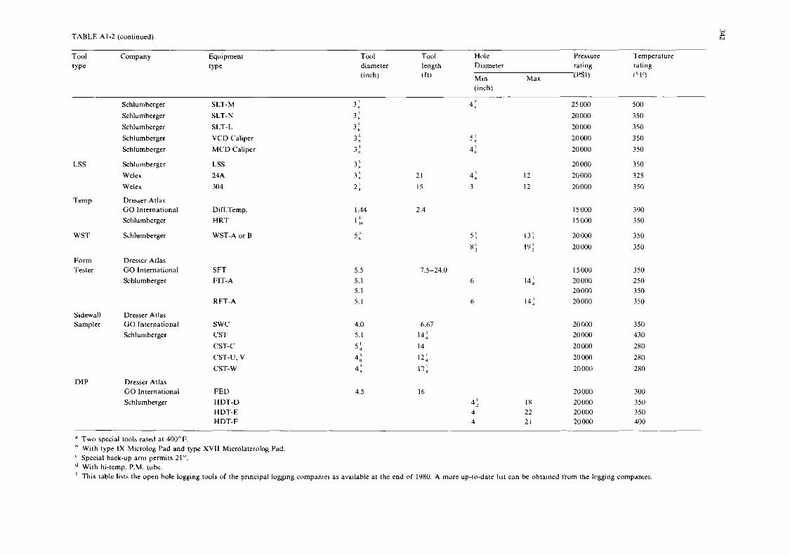
TABLE AI-2 (continued)
Tool Company Equipment Tool Tool Hole Pressure Temperature type type diameter length Diameter rating rating
(inch) ( f t ) Min Max (PSI) (OF) (inch)
w P N
LSS
Temp.
W ST
Form Tester
Sidewall Sampler
DIP
Schlumberger Schlumberger Schlumberger Schlumberger Schlumberger
Schlumberger Welex Welex
Dresser Atlas GO International Schlumberger
Schlumberger
Dresser Atlas GO International Schlumberger
Dresser Atlas GO International Schlumberger
Dresser Atlas GO International Schlumberger
SLT-M SLT-N SLT-L VCD Caliper MCD Caliper
LSS 24A 304
Diff.Temp. H RT
WST-A or B
SFT FIT-A
RFT-A
swc CST CST-C CST-U. V CST-W
FED HDT-D HDT-E HDT-F
3: 3; 3: 3: 3:
3: 3: 2:
1.44
1 I:. 5:
5.5 5. I 5.1 5.1
4.0 5.1
5: 4: 4:
4.5
21 15
2.4
4:
5: 4:
4: 3
5; 81
7.5-24.0 6
6
6.67 14: 14 12: I?:
16 4; 4 4
12 12
14:
14:
25 000 20 000 20000 20 000 20 000
20 000 20000 20000
15 000 15 000
20 000 20 000
I5 000 20 000 20 000 20000
20 000 20 000 20 000 20 000 20 000
20 000 18 20 000 22 20000 21 20 000
500 350 350 350 350
350 325 350
390 350
350 350
350 250 350 350
350 430 280 280 280
300 350 350 400
a Two special tools rated at 400°F. With type IX Microlog Pad and type XVlI Microlaterolog Pad. Special back-up arm permits 21". With hi-temp. P.M. tube.
I This table lists the open hole logging tools of the principal logging companies as available at the end of 1980. A more up-to-date list can be obtained from the logging companies.
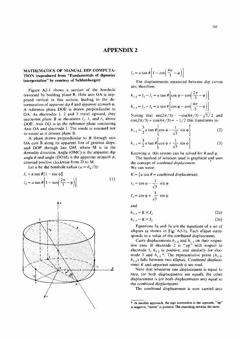
343
APPENDIX 2
MATHEMATICS O F MANUAL DIP COMPUTA- TION (reproduced from “Fundamentals of dipmeter interpretation” by courtesy of Schlumberger)
Figure A2-1 shows a section of the borehole traversed by bedding plane B. Hole axis OA is sup- posed vertical in this section, leading to the de- termination of apparent dip 8 and apparent azimuth cp. A reference plane DOF is drawn perpendicular to OA. As electrodes 1, 2 and 3 travel upward, they encounter plane B at elevations I , , I, and I, above DOF. Axis OD is in the reference plane containing Axis OA and electrode 1. The sonde is assumed not to rotate as it crosses plane B.
A plane drawn perpendicular to B through axis OA cuts B along its apparent line of greatest slope, and DOF through line OM, where M is in the downdip direction. Angle (OMC) is the apparent dip angle B and angle (DOM) is the apparent azimuth cp, counted positive clockwise from D to M.
I, = a t a n 8 [ 1 -cos+]
Let a be the borehole radius ( a = d J2):
I A
1, = a tan o [ 1 - cos( $ - $11 The displacements measured between dip curves
are, therefore:
h , - , = I , - 1, = a tan B cos cp - cos - - cp [ (‘3” 11 h, .3 = I , - I , = a tan 0 cos cp - cos - - [ (“3” $11 Noting that s in(2~/3) = - sin(4~/3) = d v 2 and cos(2a/3) = cos(4~/3) = - 1/2 this transforms to:
(3)
Knowing a , this system can be solved for 8 and cp.
the concept of combined displacement. We can write:
K = $ a tan 8 = combined displacement.
The method of solution used is graphical and uses *
1 . Z, = cos q~ - - sin cp 0 1 . Z, = cos cp + - sin cp
and h, . , = K X I ,
h , - 3 = K x I,
0
Equations 2a and 3a are the equations of a set of ellipses as shown in Fig. A3-la. Each ellipse corre- sponds to a value of the combined displacement.
Carry displacements h 1 - , and h , - 3 on their respec- tive axes. If electrode 2 is “up” with respect to electrode 1, h , - , is positive, and similarly for elec- trode 3 and h, .3 *. The representative point ( A l . * , h ,-,) falls between two ellipses. Combined displace- ment K and apparent azimuth C#I are read.
Note that whenever one displacement is equal to zero, (or both displacements are equal), the other displacement is (or both displacements are) equal to the combined displacement.
The combined displacement is now carried into
* In another approach, the sign convention is the opposite, “up” is negative, “down” is positive. The reasoning remains the same.

344
Fig. A3-lb which solves the equation:
K = +a tan 8
Example: data of Appendix 3, Method 1. Displacement between curves:
Curves I and 3 3 up = 1.5 mm Figure A3-la gives K = 2.65 mm on 1/20 scale So on scale 1: K = 2.65 X 20 = 53 mm and a = 4.125 X 25.4
= 104.775 mm. So we have: 2 K 106 3a 314.325
tan 8 = - = ~ - - 0.33723 for 8, the apparent dip
which gives:
Curves I and 2 2 up = 3.0 mm e = 18038’ as apparent dip. Compare with graphical methods explained in Ap- pendix 3.
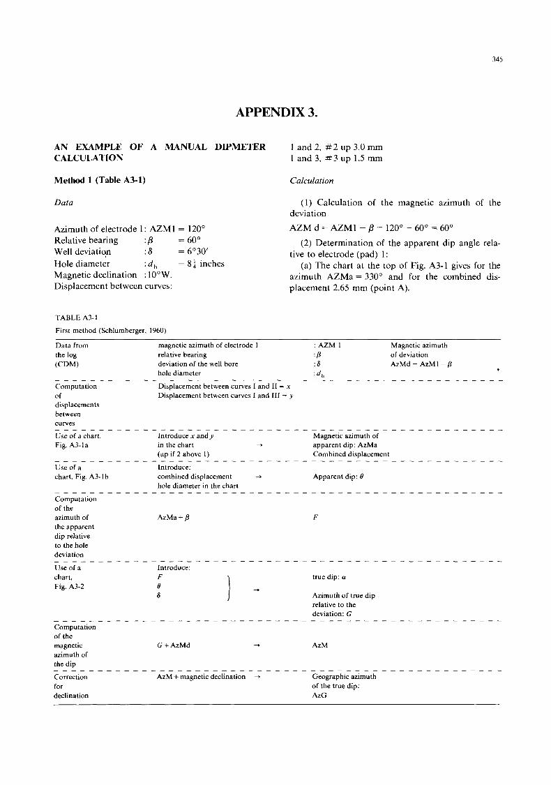
345
APPENDIX 3.
AN EXAMPLE OF A MANUAL DIPMETER CALCULATION
Method 1 (Table A3-1)
Data
Azimuth of electrode 1: AZMl = 120' Relative bearing : P = 60" Well deviation :s = 6'30' Hole diameter : d , = 8; inches Magnetic declination : 1O"W. Displacement between curves:
TABLE A3-I
First method (Schlumberger, 1960)
1 and 2, #2 up 3.0 mm 1 and 3, # 3 up 1.5 mm
Calculation
(1) Calculation of the magnetic azimuth of the deviation AZM d = AZMl - /3 = 120" - 60" = 60"
(2) Determination of the apparent dip angle rela- tive to electrode (pad) 1:
(a) The chart at the top of Fig. A3-1 gives for the azimuth AZMa = 330" and for the combined dis- placement 2.65 mm (point A).
Data from magnetic azimuth of electrode I : AZM 1 Magnetic azimuth the log relative bearing : P of deviation
hole diameter : d ,
Displacement between curves I and I1 = x
(CDM) deviation of the well bore : 6 AzMd = AzMl - /3 b
_ - _ - _ _ _ - _ - - _ - _ - - - - _ - - - - _ - - - - _ - - - - - - - - - - _ - _ _ - - - - _ - - - Computation of displacements between curves
Use of a chart, Introducex a n d y Magnetic azimuth of
Displacement between curves I and I11 = y
_ - _ - _ _ _ - _ _ - _ - _ - - - - _ - - - - - - - - - _ - - - - _ - - _ - - - - - - -
chart, Fig. A3-2
_ - _ _ - _ _ - _ - - Computation of the magnetic azimuth of the dip
Correction for declination
_ _ _ _ _ _ _ - _ _ _
G + AzMd * AzM
of the true dip: AzG
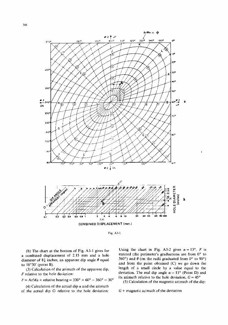
346
+ 2 + UP jlMa= +
a
.
16 14 12
J i I4
6
I 0.1 0:2 9; 4 4 0,6 0:e i 2 3 4 6 a 1 0 20 30 4 0 60 80100
2 6 5
COMB I N ED D I SP LAC EM E NT ( mm .)
a w c
b
Fig. A3-1
(b) The chart at the bottom of Fig. A3-1 gives for a combined displacement of 2.15 mm and a hole diameter of 8a inches, an apparent dip angle 8 equal to 18'30' (point B).
(3) Calculation of the azimuth of the apparent dip, F relative to the hole deviation: F = AzMa + relative bearing = 330" + 60" - 360" = 30"
(4) Calculation of the actual dip a and the azimuth of the actual dip G relative to the hole deviation: -
Using the chart in Fig. A3-2 gives a = 13'. F is entered (the perimeter's graduations are from 0" to 360") and 8 (on the radii graduated from 0" to 90") and from the point obtained (C) we go down the length of a small circle by a value equal to the deviation. The real dip angle a = 13' (Point D) and its azimuth relative to the hole deviation, G = 45"
( 5 ) Calculation of the magnetic azimuth of the dip:
G + magnetic azimuth of the deviation
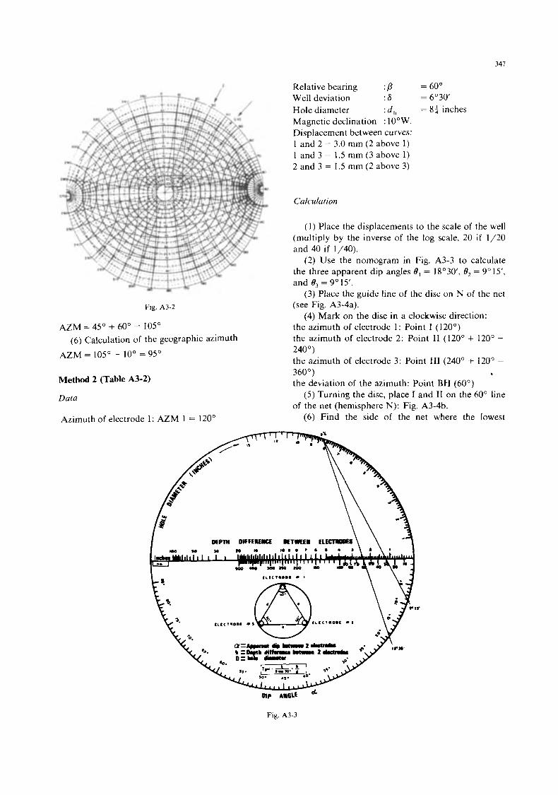
341
F
Fig. A3-2
AZM = 45" + 60" = 105" (6) Calculation of the geographic azimuth
AZM = 105" - 10" = 95"
Method 2 (Table A3-2)
Data
Azimuth of electrode 1: AZM 1 = 120"
Relative bearing : P = 60" Well deviation :6 = 6'30' Hole diameter : d , = 8a inches Magnetic declination : 1O"W. Displacement between curves: 1 and 2 = 3.0 mm (2 above 1) 1 and 3 = 1.5 mm (3 above 1) 2 and 3 = 1.5 mm ( 2 above 3)
Calculation
(1) Place the displacements to the scale of the well (multiply by the inverse of the log scale, 20 i f 1/20 and 40 i f 1/40).
(2) Use the nomogram in Fig. A3-3 to calculate the three apparent dip angles 8, = 18"30', d2 = 9"15', and 8, = 9" 15'.
(3) Place the guide line o f the disc on N of the net (see Fig. A3-4a). (4) Mark on the disc in a clockwise direction:
the azimuth of electrode 1: Point I (120") the azimuth of electrode 2: Point I1 (120" + 120" =
240") the azimuth of electrode 3: Point I11 (240" + 120" =
360") * the deviation of the azimuth: Point BH (60")
o f the net (hemisphere N): Fig. A3-4b. ( 5 ) Turning the disc, place I and I1 on the 60" line
(6) Find the side of the net where the lowest
DEPTH DIFFEREEICE BETWEEN EL-
Fig. A3-3
348
TABLE A3-2
Second method using a stereogram
Computation of (1 ) displacement between: curves I and I1 X
between curves curves I1 and I11 2
displacements curves I and 111 Y
(2) Conversion of the displacements x , y and z to the scale of the well (multiply by the inverse of the log (scale) . . . . . . . . . . . . . . . . . . . . . .
Introduce:
a b C
nomogram, a , b and c Fig. A3-3
Use of a stereogram
hole diameter in the nomogram
see Fig. A3-4 . . . . . . . . . . . . . . . . . . . . . . . . . . . . . . . . . . . . . . . . . . . . . . . . . . .
a
Fig. A3-4
349
NM magnetic azimuth of the actual dip (Fig. A3-4f): AZM = 105"
(14) Bring the guideline onto the declination NM/NG by turning the disc in the direction of the declination (towards the west in this case) by a value equal to the angle of declination and read off the position of the arrow the geographical azimuth of the actual dip: AZG = 95"
Method 3 (Table A3-3)
The same data as in Method 1 are used.
Calculation
Fig. A3-5 (1) and (2) the same as in Method 1.
electrode is located and measuring across the E-W axis of the net mark the Point A corresponding to a
Graphical (Fig. A3-5,
distance 8: Fig. A3-4b. (7) Repeat steps 5 and 6 for the set 1-111 and 8,
giving Point B and the set 11-111 and O3 giving Point C
(1) We plot the magnetic azimuth of the deviation:
AZMd = 60" (OD) (Fig. A3-4c).
(8) Turning the disc bring BH to the E-W axis (Fig. A3-4d).
(9) On the disc move the points A, B and C along small circles of the net in the direction of BH by quantities equal to the well deviation so giving points A', B', and C' (Fig. A3-4d).
(10) Turn the disc to bring A', B' and C' onto a great circle of the net (Fig. A3-4e).
( I I ) Draw an arrow on the disc along the E-W axis from the common great circle and towards the edge of the net.
(12) Read off the dip angle a by counting the number of degrees from the edge of the net to the common great circle: a = 13"
(13) Turn the disc to bring the guide line to N and read off the position of the azimuth arrow giving the
TABLE A3-3
Third method (Ref. SPE 7067, Nov. 1955; Ref. SPE 7071, Nov. 1955)
( 2 ) Plot the magnetic azimuth of the apparent dip AZMa = 330" + 120' = 90" b
(3) Plot the value of the deviation 6 (6 = 6'30') in the opposite direction to the deviation azimuth and using an arbitary scale (Point A).
(4) From this point A trace a vector parallel to the magnetic azimuth of the apparent dip AZMa on which we plot using the same scale the value of the apparent dip: point B (18'30').
(5) Trace the vector OB which gives the magnetic azimuth of the actual dip (105" on the circle).
(6) Converting the length OB, using the same scale as above, into degrees gives the actual dip angle (13").
(7) We calculate the geographical azimuth AZG of the dip by subtracting the magnetic declination
AZG = 105" - 10' = 95"
Define
Use a simplified graphical construction. Fig. A3-5 to determine AzM and a
Correction for declination
AzMa and B as in first method
AzM +magnetic declination + AZG
350
APPENDIX 4
QUICK-LOOK METHOD TO DETERMINE THE DIP AZIMUTH
,401 4 8 1 4 @ 1 4 @ 4@14@1
3 3 3 3 3 3
4@1
i
1 1 1
3
1
4@1
i
1 1 1 . 1
4@1 4(9? 4(431 3 3 3 3
0 means no shift relative to curve 1. U means “up” relative to curve 1. D means “down” relative to curve 1. To determine the dip azimuth add azimuth of electrode 1. the angle between electrode 1 and arrow. and the magnetic declination.
35 1
APPENDIX 5
QUALITY CONTROL OF LOG MEASURE- MENTS
As logs are used as the basis for a certain number of applications and are often used as a reference document for a well by the addition of other data it is important that their quality should be as high as possible, both in their technical values and in their presentation. There is therefore a need for a sys- tematic method of log quality control. It is obvious that any log interpretation and action decided upon using that interpretation will be false if the logs are bad.
An aid to the maintenance of good quality logs is to perform a series of calibrations before and after the actual logging operation. These calibrations (and their recording) help to check that the tools are functioning properly and that the various circuits and sensors are calibrated to read properly under test conditions. We should note that it is quite possible to have good calibrations but the log itself may be bad. This results from the position in the chain of sensors-circuit-recording where the calibration check occurs.
In general there are two kinds of calibration: (a) “Shop” or “Master” calibrations usually made
at the Service company workshops and involving the use of primary calibration standard or representing a primary A.P.I. standard.
(b) Wellsite calibrations. These generally include: (1) surface calibrations made before entering the well; ( 2 ) downhole calibrations; and (3) after-survey calibrations.
In each case the following points should be checked: (1) the mechanical position of the galvanometers corresponding to no signal being fed to the camera; (2) the electrical zero usually corre- sponding to no signal being fed to the measurement circuits; and (3) the calibration value resulting from a known signal source or a known calibration standard.
These calibration measurements are recorded on film at the beginning and at the end of the logging operation. In the case of computers controlled log- ging units (e.g. the Schlumberger CSU) the presen- tation of calibration data is entirely different and separate quality controls need to be established.
As a further check to log quality a repeat section is recorded over a section of the main log. This is designed to check the repeatability of and to detect erroneous shifts in the measurement. Repeat sections
should: (a) include a section covering an interval of 100
feet or 30 meters minimum; (b) include a depth mark; (c) be recorded to include both a section with
memorisation and a section without (this checks that the memorizer panel does not introduce an electrical
(d) be recorded with the same parameters as the main log including scale, logging speed, time constant etc;
(e) be identical with the main log except for statis- tical variation occurring in radioactivity logging. Repeat sections are generally recorded at the bottom of the hole but another zone can be chosen either because it is a zone of interest or because it includes good contrasts in log values.
Service and oil companies usually give their en- gineers general guidelines for quality control for each tool. It is a good idea to have a look at these. However, in order to help the geologist, it has seemed useful to gather an example of each repeat section and calibration for each of the Schlumberger tools. (These are non-CSU examples).
Finally we’note some general recommendations.
shift);
GENERAL RECOMMENDATIONS COVERING ALL OPERATIONS
The “Company” man’s wellsite responsibility
For anyone given the job of watching logging operations the following responsibilities apply: com- pany representation, control, coordination and infor- mation.
In representing the company it is not only neces- sary to know the reasons why logs are being run, the problems that can arise and how to solve them, but also to be aware of and to use with some discretion his powers of decision throughout the entire opera- tion (day and night).
General or specific guidelines for each log are not intended to reduce the material responsibilities for control and coordination of operations. Instead they are supposed to provide a framework to which are added those human qualities that should be displayed by an observer in these circumstances: adaptability, common sense, etc.
A wellsite observer is considered to have fulfilled
352
his obligations when his company both locally and centrally has information on the operation that is both complete and objective. Just filling in the boxes on a form does not immediately imply that the infor- mation is objective; some other added remarks may make the situation clearer.
Problems of security and safety of personnel de- pend on the regulations in force at the wellsite. For equipment this is the responsibility of the oil com- pany or operator in charge.
One “established” rule puts this in perspective-all contractor equipment lost or damaged at a wellsite unless it is clearly the fault of the contractor’s person- nel may be charged to the oil company or operator.
When a tool or cable is stuck in the well the contractor furnishes a “fishing” kit with suitable adaptors and recommends a method to follow. A fishing kit should be kept in each logging unit. The drilling department actually takes charge of the fish- ing operations.
Starting a logging operation
(a) Call-out of the logging team
The logging contractor should arrive sufficiently well ahead of time to avoid any downtime of the rig.
( 1) Defining the operation: this implies stipulating the logs to be run and the additional equipment needed (blowout-preventors, riser, etc.) with reference to the established well program. At this stage it should be decided which are strictly essential logs and which are optional.
(2) Keep in touch with the availability of logging equipment (via the contractor).
(3) Take into account the limitations of each tool by consulting the technical specifications given by the contractor. In, particular, the contractor should be notified if the temperature exceeds 250°F ( 120”C), the pressure is above 10,000 PSI (700 kg/cm) or if the well is highly deviated.
(4) Take into account the economic implications of each request: decide on the particular combination of logging tools to save time; and avoid duplication of curves unless they are necessary to provide quality control or indicate that the tool is functioning prop- erly (for example the caliper where a pad tool is used).
(b) Coordination with drilling or production depart- ments
(1) Ensure that the drillers and the logging com-
(a) Make sure that the well is drilled deep enough so that the top-most sensor in the log- ging string can reach the bottom-most zone of
pany are co-ordinated.
interest. For this the logging company should provide the measured distance from the sensors to the bottom of the tool string. (b) Keep in touch with any changes in mud properties that will affect the logging operation. In the case of electrical logs of all kinds (ES, IES, LL, ML, MLL, SFL, HDT) the mud type and salinity will be critical. In addition changes in mud properties that occur after drilling a section but before logging might mean that the fluid in the invaded zone bears no relationship to that measured by the logging engineer just before logging. Changes in the SP and other logs will result. (c) Make decisions with the drillers and logging
engineers on the condition of the hole and the need for wiper trips and so on. I t is particularly important not to run some types of tools in adverse hole conditions.
(2) In all operations where a well is to be completed someone from the Production Service should be present to ensure the safety of the opera- tion, the opening and closing of flowline valves, pressure measurements and so on. The logging “ob- server” can play the role of an “intermediary” i f necessary. 8
Operations preceeding logging
(1) Documents to prepare: -a control record of logs and calibrations; -a price list (for invoicing); -logs at 1/200 scale already recorded in the same
-logs from nearby wells; -information required to complete the log head-
well;
ings; . name of the field or country; . well name; . well-co-ordinates; . depths and their source (driller, logging etc.); . mud properties (density, pH, viscosity, water
. bit size;
. casing sizes and depths, and casing weight;
. tubing (if any) sizes, weights, depths;
. deviation expected.
loss);
-relevant data on the well, drilling history, changes in mud, lost circulation zones, zones that flowed, hydrocarbon shows, lithological description from cut- tings or coring, test results, etc.
(2) Request a sample, of mud, mud filtrate and mudcake, taken using mud from the flowline just before circulation ceases before logging. These sam- ples should be given to the logging engineer to mea- sure R,, R , , and Rmc.
353
(3) In the case of a floating rig ensure that a wave-motion-compensating device has been correctly installed.
(4) Give the orders of the logs to be run not forgetting that:
(a) Some logs can only be run once results from other logs have been obtained. In this case it is best to run these logs first and then run other logs which give time to interpret the first set. (b) A tool containing a radioactive source
should never be run first in open hole because of the risk of getting stuck. (c) When hole conditions are poor it is best to run the more difficult tools first (1.e. long tools, tools with centralizers) in order to avoid making a wiper trip in the middle of the logging opera- tion. (d) When the bottom hole temperature is high run the most heat sensitive tools first. (e) In order to correlate one log set with a
previous set in the same well it is often a good idea to run a gamma ray tool in combination with the first tools run in the hole so that a correlation gamma-ray log can be run through casing. ( f ) To save time run in combination as much as possible those tools that need to be run slowly.
(5) Choose depth scales for logging, generally 1/200 or 1/500 with 1/40 for microtools or HDT.
General checks to be made before and during running in the hole
(a) Before running in
(1) Some tools are calibrated on surface before running in. Each of these tools has specific calibra- tion guidelines given by the logging companies and these guidelines should be verified. Check the quality of the calibration.
(2) Make sure that a maximum-reading thermome- ter is attached to each tool.
(b) While running in
(1) Choice of scale Where scales are not fixed, check while running in
the maximum and minimum log values seen and choose a scale accordingly. In some cases a back-up galvanometer is required on a particular log.
Where a first log is run on a logarithmic scale the probable position of minimum and maximum values on other logs can be produced. Note that with many tools it is not possible to see or read the progressing values while running in the hole, for example, a pad tool that is closed up.
A correctly chosen scale should show detail in readings of low amplitude. Generally a log should be kept within the film track or tracks chosen. Try to avoid frequent use of back-ups as this makes readings difficult.
Record all resistivity logs so as to have the same scale in the low resistivity track. Generally resistivity logs are all recorded on the same scale and more and more a logarithmic scale is chosen for them all. ( 2 ) Depth correlation
The first log run serves as the depth reference for all other logs. When possible correlate the first log with other logs run in preceeding log operations. I f not, depth correlates with the casing shoe. In any case check the casing shoe and the total drilling depths.
If there is a difference in the log depth and the drilling depths greater than one in a thousand, check if the error is connected with the logging operation or arises from some other local source (for example missing out one stand or joint of drill pipe in the drill-pipe tally). Check that logging depths are mea- sured with the cable under tension (logging up not down).
(3) Other checks while running in. Keep a close eye on the cable tension meter to detect when the tools hold up while running in. Check that the depth measuring wheels running on the cable turn normally and evenly with cable movement. Watch the galvanometers to see that there is movement indicat- ing that the tool is moving.
(4) When the well is very hot record logs whle running in where possible. As some tools are particu- larly temperature sensitive this is often the only way to record a log.
General checks at bottom and while logging
(a) A t bottom and before recording
( 1) Downhole calibrations: this should correspond exactly with the surface or shop (master) calibration. Check that the calibration is recorded at least on a scale of 1/200.
(2) Record zeros before recording the logs. (3) Record a repeat section (see above comments).
(b) During logging
Record zeros before logging. Note the pick-up point of each tool from the
bottom (and in the case of nuclear tools record the tension on film).
Check the logging speed. Watch the tension meter and note “sticky” points
Check the cable magnetic marks. during logging.
354
Check that the magnetic mark is consistent and that no changes are greater than lm in 100m.
Check correlation markers, ie. beds that are easily identified as depth marks, and that these are appear- ing at the correct depth.
Check memorization of one log to the reference. Check that all curves are present (back-up curves
in particular). Watch that the film turns in the film cassettes and
in the film take-up cassettes. I t can happen that the film does not turn or becomes jammed inside the camera.
Note points at which scale changes or mechanical shifts are made.
Watch out for strange effects such as galvanometer vibration, imposed periodic parasitic effects, etc.
Where possible record at least one hundred feet of overlap with previous logs.
Record all logs at least twenty meters into the casing .
Record all calibrations after logging. Develop all films immediately after the calibra-
tions are recorded. In this way if something is wrong the operation
can be restarted without further loss of time so long as the problem arises from an operator error (film not turning, recording started at the wrong depth or stopped too early, etc.).
General quality checks on recorded logs
Logging Speed Checks: a blank marker appears every one minute in the black edge of one track.
The main log and repeat section should be identi- cal except for statistical variation arising on nuclear
The calibrations and zeros recorded before and after logging should be within the tolerances pre- scribed for each tool.
logs.
Check that the memorisation is correct. Compare overlap sections with previous logging
runs. These should match in log readings and should be perfectly matched in depth.
Overlay the different logs to check depth correla- tion. In overlap sections the correlation should be good for porosity tools (FDC, SL, etc.). For resistiv- ity tools changes in invasion diameters may influence readings. However, in front of completely impermea- ble zones the logs should read the same. The same problems arise for neutron logs in front of gas-bear- ing formations.
Correlate the new logs with those recorded in nearby wells checking local markers (salt, anhydrite, coal, etc.) and also readings in shale beds and water- bearing formations.
Ensure that there are no parasitic effects by way of
superimposed periodic signals, kicks on the logs or galvanometer vibrations.
Check that all curves are present. Check that all depth and grid lines are present. Check that the film is correctly developed and that
the traces are clearly seen, particularly in the case of micro-resistivity logs.
If there is any doubt about the quality of a log the logging engineer should try to find its cause and following consultation with the operation supervisor, rerun the log if necessary.
If the rerun is still unsatisfactory or the original fault is traced to a tool fault immediate action should be taken to bring in a replacement tool or to repair the tool in such a way that the loss of rig time is minimized. Generally one tool can be repaired or iq 'aced while other services are being run.
When the tool is brought out of the hole ensure that the pads, back-up arms, centralizers, etc. are all in place and that nothing has been left in the hole.
Checks on log headings and prints
Check that log headirgs are correctly filled in with hole information, equipment types, stand-off or centralizer information, mud characteristics, mention of other logs run in the same series of generations, the maximum temperature, R , at that temperature and general comments.
Check that all scale changes and mechanical shifts are noted on the film.
Make sure that a note 1s made on the heading or film of all data relating to tool sticking, problems with the recording camera, loss of one or more curves on the film for whatever reason, etc.
In the case of some logging operations (e.g. pro- duction logging) make sure that the exact sequence of operations is noted on the heading.
Check that the headings of composite logs made up of several logging runs contains all the informa- tion relating to each individual run.
Check print quality.
Reports at the end of logging
This report is made up of two parts: (a) A sheet detailing operations. This document
should be completed by the engineer and the opera- tion supervisor. It should: (b) allow the proper in- voicing of the operation; and (c) give a recap of the logs noting any anomalies in recording or quality.
(b) A complete interpretation report of the opera- tion in four parts: (1) a detailed qualitative study; (2) the lithological report of the logged section; (3) corre- lations with neighbouring wells; and (4) a quantita- tive evaluation of the reservoirs.
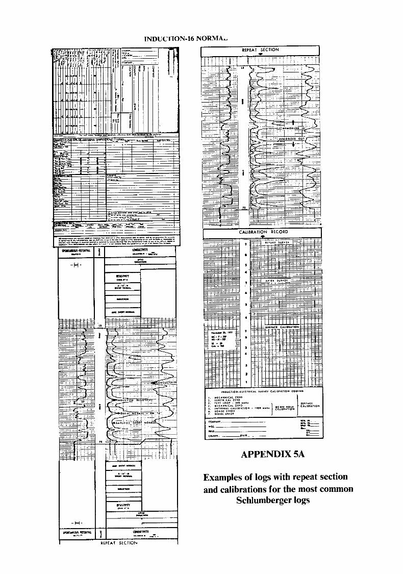
INDUCTION-16 NORMA,
~
-H*
-H*
1 no .oMoI I I
I REPEAT SECTION 1
CALIBRATION RECORD
APPENDIX 5A
Examples of logs with repeat section and calibrations for the most common
Schlumberger logs
351
INDUCTION - SPHERICALLY FOCUSED LOG SONIC
r REPEAT S E C V O N 1
I J NO11335 lV3d3U
301 A.LIMIIXO2Id-30702I3IMI
GAMMA RAY-NEUTRON GNT
REPEAT SECTION
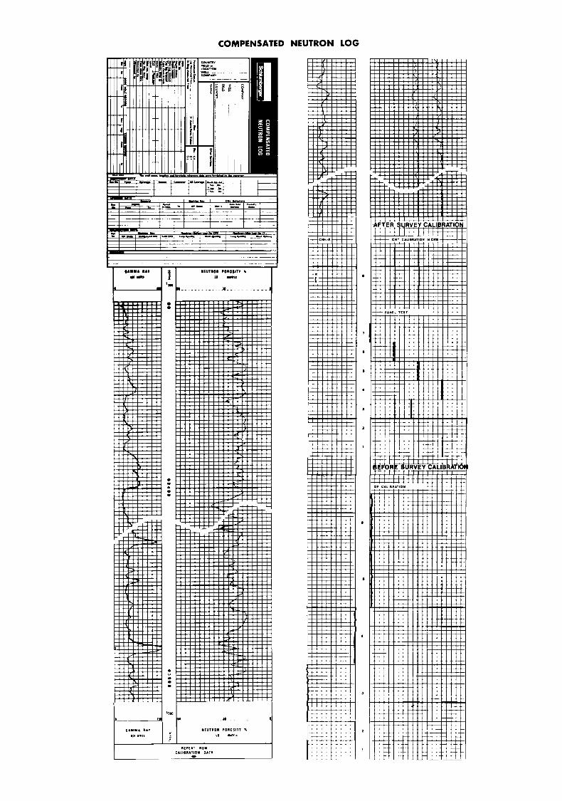
Y
CNT-A
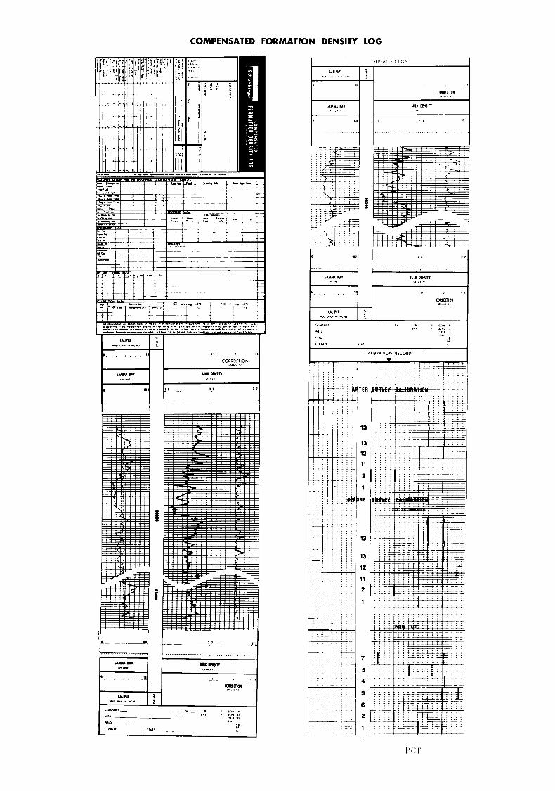
PGT
GAMMA RAY-BOREHOLE
Le -
I
i
S
' I
.-- I D
H I 1 A ..
COMPENSATED SONIC
I REPEAT SECTION 1
HDT-D/E
I REPEAT SECTION 1
w . . r I
CEMENT BOND LOG
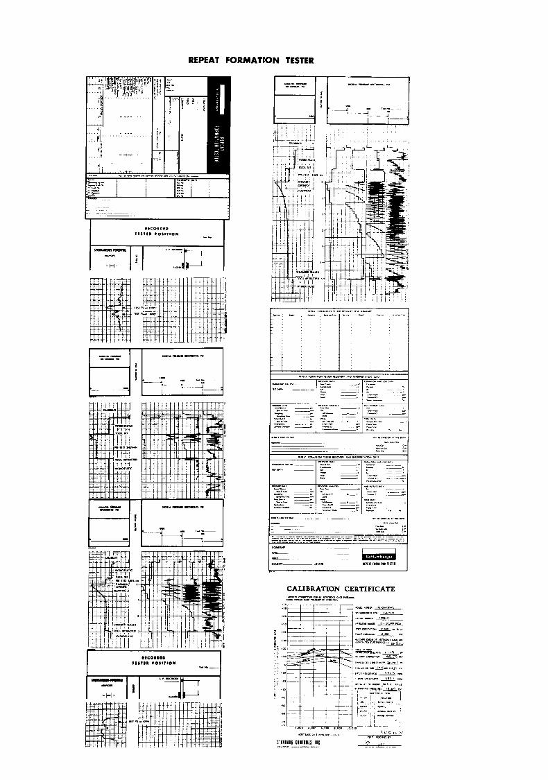
REPEAT FORMATION TESTER
I . . . . . ....,... . ;:I1
t i
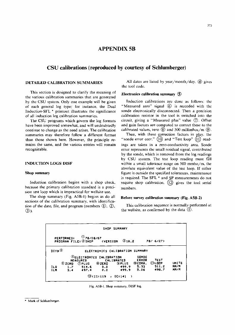
373
APPENDIX 5B
CSU calibrations (reproduced by courtesy of Schlumberger)
DETAILED CALIBRATION SUMMARIES
This section is designed to clarify the meaning of the various calibration summaries that are generated by the CSU system. Only one example will be given of each general log type; for instance, the Dual Induction-SFL * printout illustrates the significance of all induction log calibration summaries.
The CSU programs which govern the log formats have been improved somewhat, and will undoubtedly continue to change as the need arises. The calibration summaries may therefore follow a different format than those shown here. However, the principle re- mains the same, and the various entries will remain recognizable.
INDUCTION LOGS DISF
Shop summary
Induction calibration begins with a shop check, because the primary calibration standard is a preci- sion test loop which is impractical for wellsite use.
The shop summary (Fig. A5B-1) begins as do all sections of the calibration summary, with identifica- tion of the date, file, and program (numbers 0, 0, 0 ).
All dates are listed by year/month/day. @ gives the tool code.
Electronics calibration summary @
Induction calibrations are done as follows: the “Measured zero” signal @ is recorded with the sonde electronically disconnected. Then a precision calibration resistor in the tool is switched into the circuit, giving a “Measured plus” value 0. Offset and gain factors are computed to correct these to the calibrated values, zero @ and 500 millimhos/m @.
“sonde error corr.” @ and “Test loop” g i e : ings are taken in a zero-conductivity area. Sonde error represents the small residual signal, contributed by the sonde, which is removed from the log readings by CSU system. The test loop reading must fAII within a small tolerance range on 500 mmho/m, the absolute equivalent value of the test loop. If either figure is outside the specified tolerances, maintenance is required. The SFL * and SP measurements do not require shop calibration. @ gives the tool serial numbers.
Then, with these correction factors in
Before survey calibration summary (Fig. A5B-2)
the wellsite, as confirmed by the data 0. This calibration sequence is normally performed at
SHOP SUMMARY
PERFORMED: @78/08/07 PROGRAM FILE: @SHOP (VERSION 010.2 78/ 6/27)
DITP@ ELECTRONICS CALIBRATION SUMMARY
@ELECTRONICS CAL IBRATION SONDE MEASURED CALIBRATED ERROR TEST
ILD 1.7 514.6 0.0 499.9 5.33 511.2 MM/M I L M 3.4 497.4 0.0 499.9 5.06 498.7 MH/M
@ZERO @PLUS @ZERO @PLUS @CORR. @LOOP UNITS
@(IS1119 IC1141 )
Fig. A5B-1. Shop summary, DISF log.
* Mark of Schlumberger.
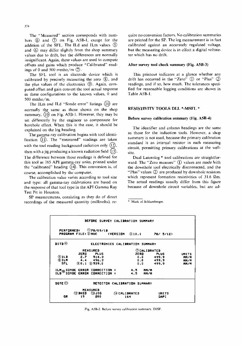
314
The “Measured” section corresponds with num- bers @ and 0 on Fig. A5B-1, except for the addition of the SFL. The ILd and ILm values @ and @ may differ slightly from the shop summary values due to drift, but the differences are normally insignificant. Again, these values are used to compute offsets and gains which produce “Calibrated” read- ings of 0 and 500 mmho/m 0.
The SFL tool is an electrode device which is calibrated by precisely measuring the zero @, and the plus values of the electronics a. Again, com- puted offset and gain convert the tool actual response in these configurations to the known values, 0 and 500 mmho/m.
The ILm and ILd “Sonde error” listings @ are normally the same as those shown on the shop summary, @ on Fig. A5B-1. However, they may be set differently by the engineer to compensate for borehole effect. When this is the case, it should be explained on the log heading.
The gamma-ray calibration begins with tool identi- fication 0. The “measured” readings are taken with the tool reading background radiation only 12 , then with a jig producing a known radiation field 8 13 . The difference between those readings is defined for this tool as 165 API gamma-ray units, printed under the “calibrated” heading 0. This conversion is, of course, accomplished by the computer.
The calibration value varies according to tool size and type: all gamma-ray calibrations are based on the response of that tool type in the API Gamma Ray Test Pit in Houston.
SP measurements, consisting as they do of direct recordings of the measured quantity (millivolts), re-
quire no conversion factors. No calibration summaries are printed for the SP. The log measurement is in fact calibrated against an accurately regulated voltage, but the measuring device is in effect a digital voltme- ter which has no drift.
After survey tool check summary (Fig. A5B-3)
This printout indicates at a glance whether any drift has occurred in the “Zero” @ or “Plus” 0 readings, and if so, how much. The tolerances speci- fied for reasonable logging conditions are shown in Table A5B-1.
RESISTIVITY TOOLS DLL *-MSFL *
Before survey calibration summary (Fig. A5B-4)
The identifier and column headings are the same as those for the induction tools. However, a shop summary is not used, because the primary calibration standard is an internal resistor in each measuring circuit, permitting primary calibrations at the well- site.
Dual Laterolog * tool calibrations are straightfor- ward. The “Zero measure” @ values are made bith the downhole tool electrically disconnected, and the “Plus” values 0 are produced by downhole resistors which represent formation resistivities of 3 1.6 Qm. The actual readings usually differ from this figure because of downhole circuit variables, but are ad-
* Mark of Schlumberger.
BEFORE SURVEY C A L I B R A T I O N SUMMARY
PERFORMED: 078/09/18 P R O G R M F I L E : @ N U C ( V E R S I O N @lO.l 78/ 5 / 1 2 )
DITDO ELECTRONICS C A L I B R A T I O N SUMMARY
MEASURED ZERO PLUS
OILD 2.7 514.3 QILM 4.4 496.3
SFL 0 0 . 1 B539.0
@CALIBRATED ZERO PLUS U N I T S
0 . 0 499.9 MM/M 0.0 499.9 MM/M 0.0 499.9 MM/M
I L M m S O N D E ERROR CORRECTION : 4.5 MM/M I L D SONDE ERROR CORRECTION I 4.5 MM/M
I SGTEO DETECTOR C A L I B R A T I O N SUMMARY
MEASURED OBKGD @JIG @J C A L I BRATED U N I T S
GR 19 20 0 164 GAP I
Fig. A5B-2. Before survey calibration summary. DISF.
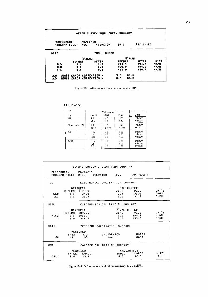
315
Log IES
AFTER SURVEY TOOL CHECK SUMMARY
PERFORMED1 7 8 / 0 9/ 18 PROGRAM F I L E 1 NUC (VERSION 10.1 78/ 5/12)
D I T D TOOL CHECK
0 ZERO 0 PLUS BEFORE AFTER BEFORE AFTER U N I T S
I L D 0 . 0 0 . 0 499.9 494.4 MM/M ILM 0 . 0 - 0 . 0 499.9 494.8 MM/M SFL 0 . 0 0 . 1 499.9 496.7 MM/M
Tolerance Curve Zero Plus Units I Ld t2 z 20 mholm SFL 22 i- 20 mholm
ILM SONDE ERROR CORRECTION I 5 . 0 MM/M I L D SONDE ERROR CORRECTION 8 8.5 MM/M
~~ _ _ _ _ _ _ ~ ~
Fig. A5B-3. After survey tool check summary, DISF.
TABLE A5B-1
I Slim Hole IES rnholm 16" N
mholm I Ld z 20 mho/m LL8 5 20 mholm
I DISF
I ILm z 2 -t 20 mholm
mholm ILd SFL 1 1 z:: 1 mholm 1
I BEFORE SURVEY C A L I B R A T I O N SUMMARY
PERFORMED: 78 / 1 0 / 1 0 PROGRAM F I L E : MILL ( V E R S I O N 1 0 . 2 78/ 6 / 2 7 )
DLT E L E C T R O N I C S C A L I B R A T I O N SUMMARY
MEASURED @ Z E R O @PLUS
L L D 0 . 0 3 4 . 5 L L S 0.0 33 .9
C A L I B R A T E D ZERO P L us U N I T S
0 . 0 3 1 . 6 OHMM 0.0 3 1 . 6 OHMM
MSFL E L E C T R O N I C S C A L I B R A T I O N SUMMARY
MEAXURED @ Z E R O @PLUS
MSFL 0 . 0 1 0 0 3 . I 1 5.8 2 0 6 . 0
@CALIBRATED ZERO PLUS U N I T S
0 . 0 999.9 MMHO 0.0 1 9 9 . 9 MMHO
SGTE DETECTOR C A L I B R A T I O N SUMMARY
MEASURED BKGD J I G CQLIBRATLD U N I T S
GR 4 3 195 1 6 4 GAP I
I MSFL C A L I P E R C A L I B R A T I O N SUMMARY
MEASURED SMALL LARGE 1 C A L I 9 . 4 1 3 . 6
C A L I B R Q T E D SMALL LARGE U N I T S
8 . 0 1 2 . 0 I N
Fig. A5B-4. Before survey calibration summary, DLL-MSFL.
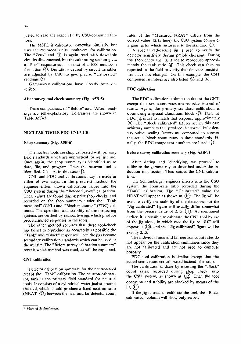
316
justed to read the exact 31.6 by CSU-computed fac- tors.
The MSFL is calibrated somewhat similarly, but uses the reciprocal units, mmho/m, for calibration. The “Zero” end @ is again read with downhole circuits disconnected, but the calibrating resistor gives a “Plus” response equal to that of a lOOO-mmho/m formation @. Deviations caused by circuit variables are adjusted by CSU to give precise “Calibrated” readings 0.
Gamma-ray calibrations have already been de- scribed.
After survey tool check summary (Fig. A5B-5)
These comparisons of “Before” and “After” read- ings are self-explanatory. Tolerances are shown in Table A5B-2.
NUCLEAR TOOLS FDC-CNL*-GR
Shop summary (Fig. ASB-6)
The nuclear tools are shop calibrated with primary field standards which are impractical for wellsite use. Once again, the shop summary is identified as to date, file, and program. Then the neutron tool is identified, CNT-A, in this case 0.
CNL and FDC tool calibrations may be made in either of two ways. In the prevalent method, the engineer enters known calibration values into the CSU system during the “Before Survey” calibration. These values are found during prior shop checks, and recorded on the shop summary under the “Tank measured” (CNL) and “Block measured” (FDC) col- umns. The operation and stability of the measuring systems are verified by radioactive jigs which produce predetermined responses in the tools.
The other method requires that these tool-check jigs be set to reproduce as accurately as possible the “Tank” and “Block” responses. Then the jigs become secondary calibration standards which can be used at the wellsite. The “Before survey calibration summary” reveals which method was used, as will be explained.
CNT calibration
Detector calibration summary for the neutron tool recaps the “Tank” calibration. The neutron calibrat- ing tank is the primary field standard for neutron tools. It consists of a cylindrical water jacket around the tool, which should produce a fixed neutron ratio (NRAT, 0) between the near and far detector count
rates. If the “Measured NRAT” differs from the correct value (2.15 here), the CSU system computes a gain factor which restores it to the standard 0.
A special radioactive jig is used to verify the detector sensitivity during prejob checkout. During the shop check the jig is set to reproduce approxi- mately the tank ratio @. This check can then be repeated in the field to verify that detector sensitivi- ties have not changed. On this example, the CNT component numbers are also listed 0 and 8.
FDC calibration
The FDC calibration is similar to that of the CNT, except that raw count rates are recorded instead of ratios. Again, the primary standard calibration is done using a special aluminium block 0. Then the FDC jig is set to match that response approximately @. The “Block calibrated” figures are in this case arbitrary numbers that produce the correct bulk den- sity value; scaling factors are computed to convert the actual block count rates to these standards. Fi- nally, the FDC component numbers are listed @.
Before survey calibration summary (Fig. A5B-7)
After dating and identifying, we proceed ’ to calibrate the gamma ray as described under the in- duction tool section. Then comes the CNL calibra- tion.
The Schlumberger engneer inserts into the CSU system the count-rate ratio recorded during the “Tank” calibration. The “Calibrated” value for NRAT will appear as shown at @. The jig will be used to verify the stability of the detectors, but the “Jig calibrated” figure will usual1 differ somewhat from the precise value of 2.15 6. As mentioned earlier, it is possible to calibrate the CNL tool by use of the jig alone, in which case the figure “0.0” will appear at @, and the “Jig calibrated” figure will be exactly 2.15.
The individual near and far neutron count rates do not appear on the calibration summaries since they are not calibrated and are not used to compute porosity.
FDC tool calibration is similar, except that the actual count rates are calibrated instead of a ratio.
The calibration is done by inserting the “Block” count rates, recorded during shop check, into the CSU system, as shown at 0. Then the tool operation and stability are checked by means of the jig 0.
If the jig is used to calibrate the tool, the “Block calibrated” column will show only zeroes.
* Mark of Schlumberger.
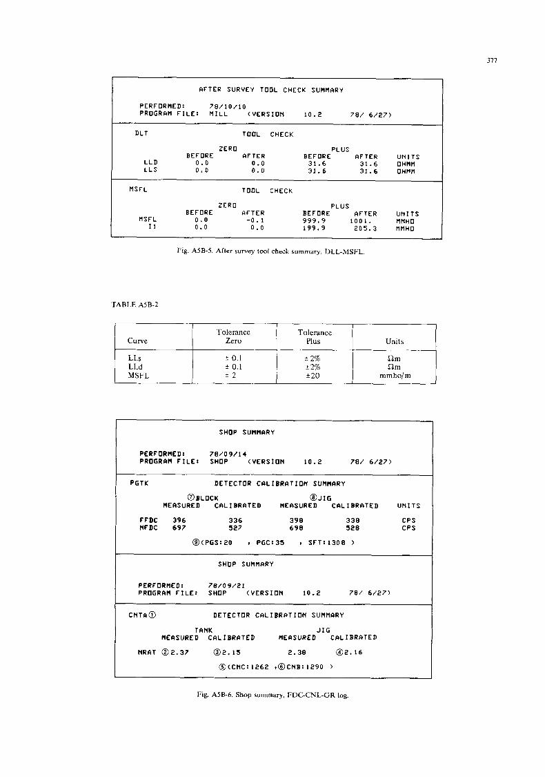
371
Tolerance Tolerance Curve Zero Plus
LLS f 0.1 * 2% LLd f 0.1 f 2% MSFL 2 2 f 20
AFTER SURVEY TOOL CHECK SUMMARY
Units
f lm f l m
mmho/m
PERFORMED: 78/10/10 PROGRAM F I L E : MILL ( V E R S I O N 10.2 78/ 6 / 2 7 )
1 DLT TOOL CHECK
ZERO PLUS BEFORE AFTER BEFORE AFTER U N I T S
L L D 0 .0 0 .0 31.6 31.6 OHMM L L S 0 . 0 0 .0 31.6 31.6 OHMM
MSFL
MSFL I 1
TOOL CHECK
ZERO PLUS BEFORE AFTER BEFORE AFTER U N I T S
0 . 0 -0 .1 999 .9 100 1. MMHO 0 . 0 0 . 0 199.9 205.3 MMHO
Fig. A5B-5. After survey tool check summary, DLL-MSFL
TABLE A5B-2
SHOP SUMMARY
PERFORMED: 78/0 9 / 14 PROGRAM F I L E : SHOP ( V E R S I O N 10.2 78 / 6 / 2 7 )
1 PGTK DETECTOR C A L I B R A T I O N SURRARY
@BLOCK @JIG MEASURED C A L I B R A T E D MEASURED C A L I B R A T E D U N I T S
FFDC 396 336 398 338 CPS NFDC 697 527 698 528 CPS
@(PGS:20 I PGC23S 9 SFT21308 )
SHOP SUMRARY
PERFORMED: 7 8 / 0 9 /21 PROGRAM F I L E : SHOP ( V E R S I O N 10.2 78 / 6 / 2 7 )
CNTAO DETECTOR C A L I B R A T I O N SUMMARY
TANK J I G MEASURED C A L I B R A T E D MEASURED C A L I B R A T E D
NRAT 0 2 . 3 7 0 2 . 1 5 2.38 0 2 . 1 6
@tCNC: 1262 ,@CNB: 1290 )
Fig. A5B-6. Shop summary, FDC-CNL-GR log.
a
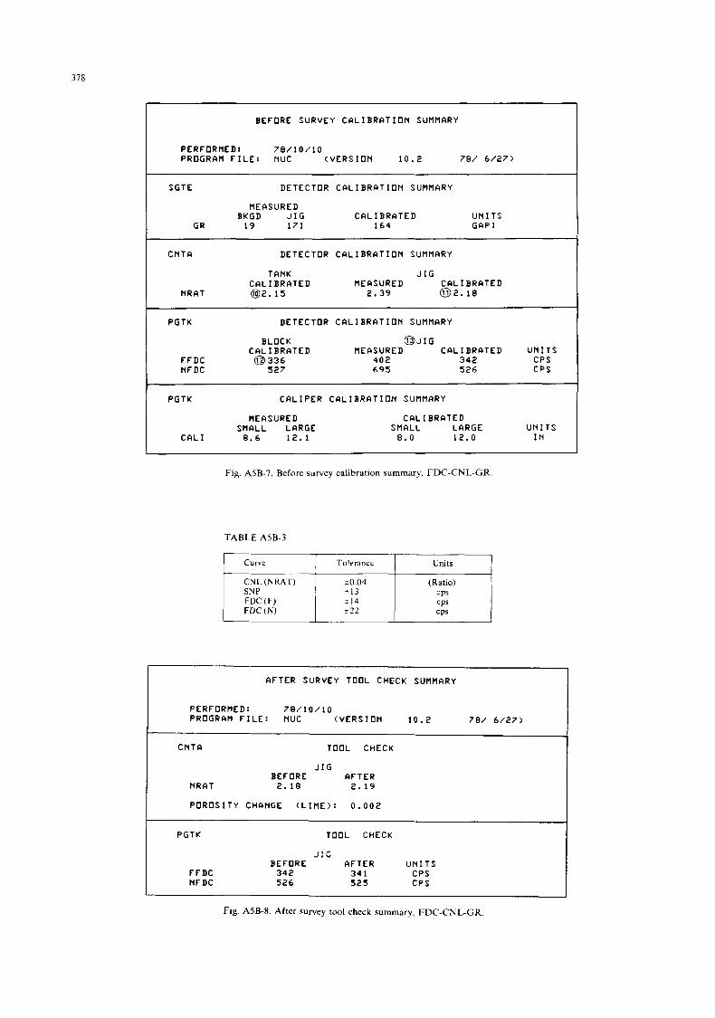
378
~~
B E F O R E S U R V E Y C A L I B R A T I O N SUMMARY
PERFORMED: 78 /10 / 10 PROGRAM F I L E : NUC ( V E R S I O N 10.2 78 / 6 / 2 7 )
S G T E D E T E C T O R C A L I B R A T I O N SUMMARY
M E A S U R E D BKGD J I G C A L I B R A T E D U N I T S
GR 19 171 164 GAP I
C N T A D E T E C T O R C A L I B R A T I O N SUMMARY
T A N K J I G C A L I B R A T E D M E A S U R E D C A L I B R A T E D
N R A T a 2 . 1 5 2.39 632 .18
P G T K
F F D C N F D C
D E T E C T O R C A L I B R A T I O N SUMMARY
B L O C K @JIG C A L I B R A T E D M E A S U R E D C A L I B R A T E D U N I T S @ 336 402 342 C P S
527 695 526 c p s
P G T K C A L I P E R C A L I B R A T I O N SUMMARY
MEASURED S M A L L L A R G E
C A L I 8.6 12.1
C A L I B R A T E D S M A L L L A R G E U N I T S
8.0 12.0 I N
Fig. A5B-7. Before survey calibration summary, FDC-CNL-GR
TABLE A5B-3
Curve Tolerance Units
CNL (NRAT) k0.04 SNP +13 FDC (F) f 14 FDC (N) ? 2 2
A F T E R S U R V E Y T O O L CHECK SUMMARY
PERFORMED: 78 /10 / 10 PROGRAM F I L E : NUC ( V E R S I O N 10.2 78 / 6 / 2 7 )
C N T A T O O L CHECK
J I G B E F O R E A F T E R
N R A T 2.18 2. 19
P O R O S I T Y CHANGE ( L I M E ) : 0 .002
P G T K TOOL CHECK
I l C d.
B E F O R E A F T E R U N I T S F F D C 342 34 1 C P S N F D C 526 525 C P S
I
Fig. A5B-8. After survey tool check summary, FDC-CNL-GR.
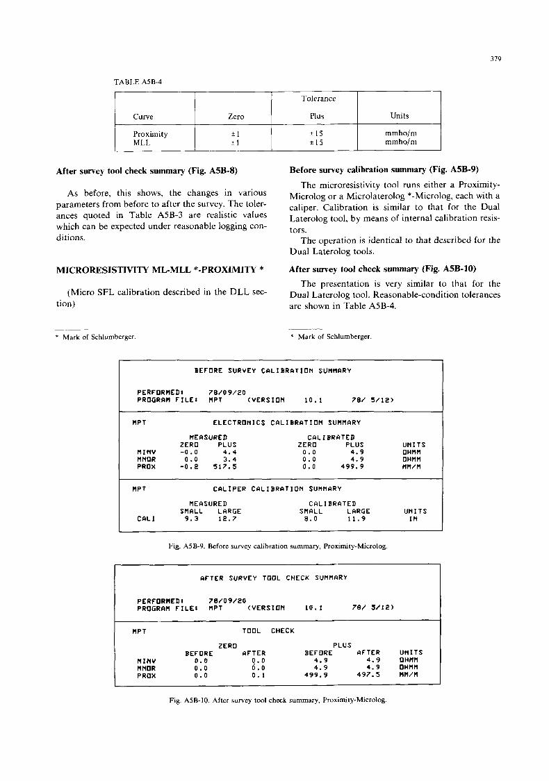
379
Tolerance
Curve Zero Plus
Proximity 2 1 5 1 5 MLL 5 1 k 1 5
Units
rnmho/rn mmho/m
After survey tool check summary (Fig. A5B-8)
As before, this shows, the changes in various parameters from before to after the survey. The toler- ances quoted in Table A5B-3 are realistic values which can be expected under reasonable logging con- ditions.
MICRORESISTIVITY ML-MLL *-PROXIMITY *
(Micro SFL calibration described in the DLL sec- tion)
Before survey calibration summary (Fig. A5B-9)
The microresistivity tool runs either a Proximity- Microlog or a Microlaterolog *-Microlog, each with a caliper. Calibration is similar to that for the Dual Laterolog tool, by means of internal calibration resis- tors.
The operation is identical to that described for the Dual Laterolog tools.
After survey tool check summary (Fig. A5B-10)
The presentation is very similar to that for the Dual Laterolog tool. Reasonable-condition tolerances are shown in Table A5B-4.
* Mark of Schlumberger. * Mark of Schlumberger.
BEFORE SURVEY C A L I B R A T I O N SUMMARY
78/09/20 PROGRFIM F I L E : MPT ( V E R S I O N 1 0 . 1 78.’ 5 / 1 2 ) I
MPT E L E C T R O N I C S C A L I B R A T I O N SUMMARY
MEflSURE D C A L I B R A T E D ZERO P L U S ZERO P L U S U N I T S
M I N V -0.0 4 . 4 0 . 0 4 . 9 OHMM BNOR 0 . 0 3 . 4 0 . 0 4 . 9 OHMM PROX - 0 . 2 517 .5 a . 0 4 9 9 . 9 MM/M
~
MPT C A L I P E R C A L I B R A T I O N SUMMARY
MEASURED SMALL LARGE
C A L I 9 . 3 1 2 . 7
C A L I B R A T E D SMALL LARGE U N I T S
8.0 1 1 . 9 I N
Fig. ASB-9. Before survey calibration summary, Proximity-Microlog.
AFTER SURVEY TOOL CHECK SUMMARY
PERFORRED: 78/09/20 PROGRAM FILE: MPT ( V E R S I O N 1 0 . 1 78/ 5/12)
MPT TOOL CHECK
ZERO P L U S BEFORE AFTER BEFORE AFTER U N I T S
M I N V 0.0 0.0 4 . 9 4 . 9 OHMM MNOR 0 . 0 0 . 0 4 . 9 4 . 9 OHMM PROX 0 . 0 0 . 1 4 9 9 . 9 497 .5 MM/M
Fig. A5B- 10. After survey tool check summary, Proximity-Microlog.

380
SONIC LOGGING galvanometers and associated circuitry, not of the measurement itself. In the CSU system, time intervals
There are no CSU system calibration summaries are keyed to a crystal-controlled oscillator, and processed in digital form; the surface equipment does not vary in sensitivity. The accuracy of the crystal clock is verified before each job.
for the sonic logs. Like the SP measurement, sonic transit-time logs are direct measurements of a basic parameter, namely time. The only calibration of con- ventional analog sonic recordings were of the
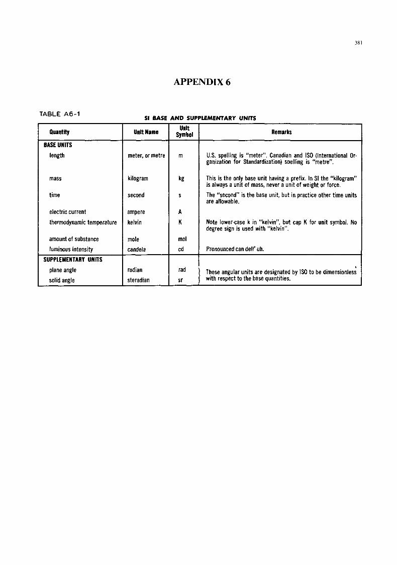
38 1
APPENDIX 6
rABLE A6-1
Quantity
BASE UNITS
length
mass
time
electric current
thermodynamic temperature
amount of substance
luminous intensity
SUPPLEMENTARYUNITS
plane angle
solid angle
51 BASE AND SUPPLEMENTARY UNITS
Unit Name
meter, or metre
kilogram
second
ampere
kelvin
mole
candela
radian
steradian
Unit Symbol
m
kg
S
A
K
mol
cd
rad
sr
Remarks
U.S. spelling is “meter”. Canadian and IS0 (International Or- ganization for Standardization) soelling is “metre”.
This is the only base unit having a prefix. In SI the “kilogram” is always a unit of mass, never a unit of weight or force.
The “second” is the base unit, but in practice other time units are allowable.
Note lower-case k in “kelvin”, but cap K for unit symbol. No degree sign is used with “kelvin”.
Pronounced can dell’ uh.
8
These angular units are designated by IS0 to be dimensionless with respect to the base quantities.
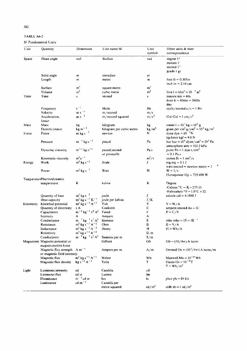
382
TABLE A6-2
SI Fundamental Units
Unit Quantity Dimension Unit name SI Unit Other units & their symbol correspondence
Space
Time
Mass
Force
Energy
Plane angle
Solid angle Length
Surface Volume Time
Frequency Velocity Acceleration, linear Mass Density (mass) Force
Pressure
Dynamic viscosity
Kinematic viscosity Work
Power
Tempera tureThermod ynamic temperature
Electricity
Magnetism
Light
Quantity of heat Heat capacity Electrical potential Quantity of electricity Capacitance Intensity Conductance Resistance Inductance Resistivity Conductivity Magnetic potential or magnetomotive force
rad
sr m
m2 m3 S
K
m2 kg sC2 m2 kg s - 2 K - ' m2 kg s - 3 A - ' s A m-2 kg-' s4 A' A m - 2 kg-' s3 A' m2 kg s-' A-' m2 kg sK2 A - 2 m' kg s-' A - 2 m - 3 kg-' s3 A2
- Magnetic flux strength or magnetic field intensity Magnetic flux Magnetic flux density
A m- ' m2 kg s -2 A - ' kg sC2 A - '
Luminous intensity cd Luminous flux cd sr Illuminance m - 2 cd sr Luminance cd m - 2
Radian
steradian metre
square metre cubic metre second
Hertz m/second m/second squared
kilogram kilogram per cubic metre newton
pascal
pascal.second or poiseuille
Joule
Watt
kelvin
joule joule per kelvin Volt Coulomb Farad Ampere Siemens Ohm Henry
Siemens per m Gilbert
Ampere per m
Weber Tesla
Candela Lumen lux Candela per metre squared
rad
sr m
m2 m3 S
Hz m/s m/s2
kg k / m 3 N
Pa
P a s
m2/s J
W
K
J
V C F A S 0 H Q . m S/m
J/K
G b
A/m
Wb T
cd Im Ix
cd/m2
degree I " minute 1' second 1" grade 1 gr
foot ft = 0.305m inch in = 2.54 cm
litre I = ldm' = 10 m3 minute mn = 60s hour h = 60mn = 3600s
cycle/second c/s = 1 Hz
Gal Gal = 1 cm/s2
tonne t = lo3 kg = lo6 g gram per cm' g/cm7 = 10' kg/m' dyne dyn = 10-5N kg-force kgf = 9.8 N bar bar = lo6 dyne/cm' = l o 5 Pa atmosphere atm = 101.3 kPa poise Po = 1 dyn s/cm2 = 0.1 Pa s
stokes St = 1 cm2/s erg erg = 0.1 J wattsecond = newton metre = J W = J/s Horsepower Hp = 735.498 W
day
'
Degree -Celsius OC = K + 273.15 -Fahrenheit O F = 1.8OC+32 calorie cal = 4.1868 J
V = W/A
F = C/V amperesecond As = IC
mho mho = IS = 1 Q - ' Q = V/A H = Wb/A
G b = ( 1 0 / 4 ~ ) A turns
Oersted Oe = (103/4n) A turns/m
Maxwell Mx = Wb Gauss Gs = 10-4T T = Wb/m2
phot ph = 10 klx
stilb sb = 1 cd/m2
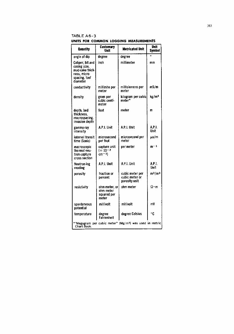
383
TABLE A 6 - 3 UNITS FOR COMMON LOGGING MEASUREMENTS I I Quantity
Caliper, bit and casing size, mudcake thick. ness, micro- spacing, tool diameter
conductivity
density
depth, bed thickness, macrospacing, invasion depth
gamma-ray intensity
interval transit time (Sonic)
macroscopic thermal neu- tron capture cross section
Neutron-log reading
porosity
resistivity
spontaneous potential
temperature
Customary Unit
degree
inch
millimho per meter
gram per cubic centi- meter
foot
A.P.I. Unit
microsecond per foot
capture unit
cm-1)
A.P.I. Unit
fraction or percent
ohm meter, c ohm meter squared per meter
millivolt
degree Fahrenheit
(= 10-3
Metricated Unit
degree
millimeter
millisiemens per meter
kilogram per cubii meter*
meter
A.P.I. Unit
microsecond per meter
per meter
A.P.I. Unit
cubic meter per cubic meter or porosity unit
ohm meter
millivolt
degree Celsius
- Unit
Symbol 0
mm
mS/m
kg/m3
m
A.P.I. Unit
&m
m-1
A.P.I. Unit
m3/mI
Clam
mV
“C
I Chart Book.
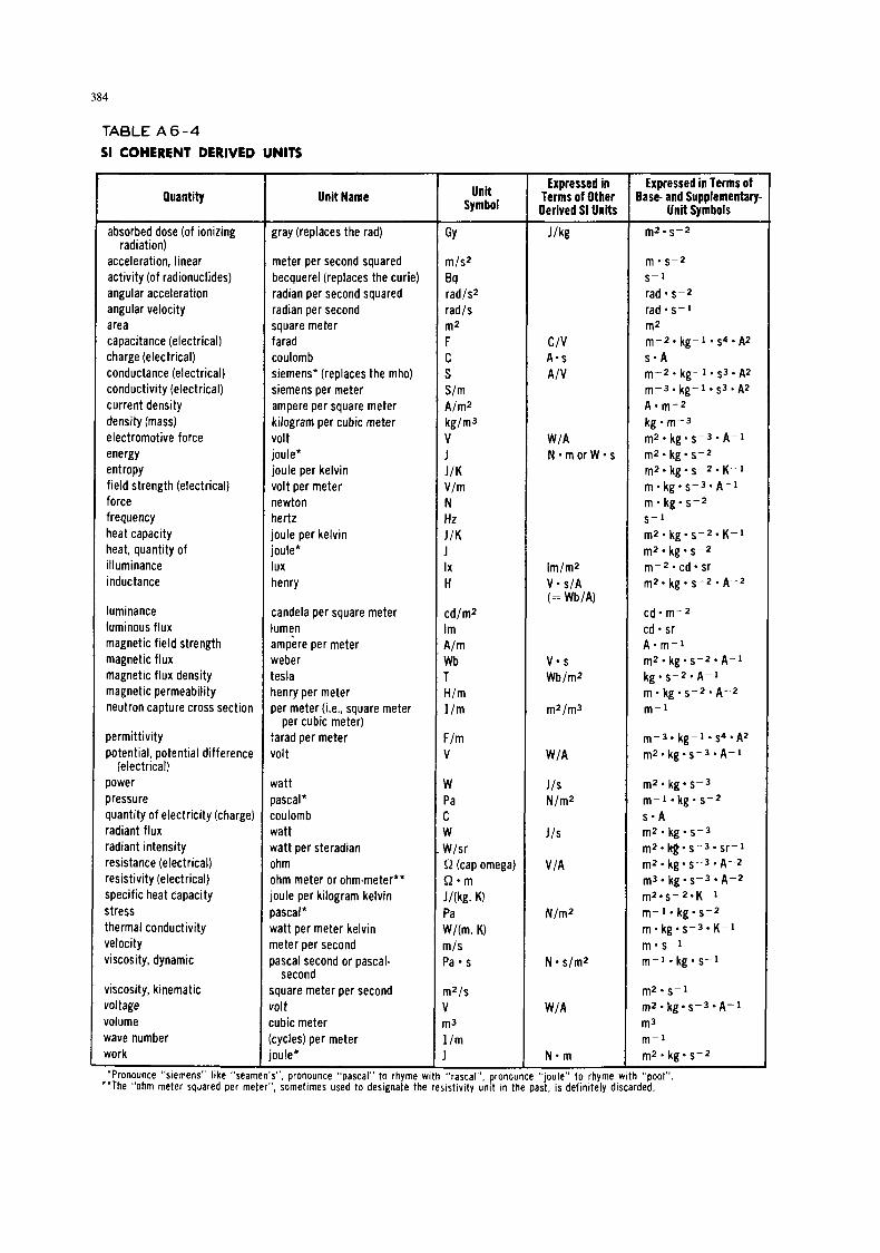
384
TABLE A 6 - 4 51 COHERENT DERIVED UNITS
Ruantity
absorbed dose (of ionizing
acceleration, linear activity (of radionuclides) angular acceleration angular velocity area capacitance (electrical) charge (electrical) conductance (electrical) conductivity (electrical) current density density (mass) electromotive force energy entropy field strength (electrical) force frequency heat capacity heat, quantity of illuminance inductance
radiation)
luminance luminous flux magnetic field strength magnetic flux magnetic flux density magnetic permeability neutron capture cross section
permittivity potential, potential difference
power pressure quantity o f electricity (charge) radiant flux radiant intensity resistance (electrical) resistivity (electrical) specific heat capacity stress thermal conductivity velocity viscosity, dynamic
viscosity, kinematic voltage volume wave number work
(electrical)
Unit Name
gray (replaces the rad)
meter per second squared becquerel (replaces the curie) radian per second squared radian per second square meter farad coulomb siemens* (replaces the mho) siemens per meter ampere per square meter kilogram per cubic meter volt joule* joule per kelvin volt per meter newton hertz joule per kelvin joule* lux henry
candela per square meter l u m y ampere per meter weber tesla henry per meter per meter (i.e., square meter
farad per meter volt
per cubic meter)
watt pascal* coulomb watt watt per steradian ohm ohm meter or ohmmeter** joule per kilogram kelvin pascal* watt per meter kelvin meter per second pascal second or pascal-
square meter per second volt cubic meter (cycles) per meter joule*
second
Unit Symbol
GY
m/s2
Bq rad/sz rad/s m2 F C S S/m A im2 kg/m3 V J J /K V i m N HZ
J / K J Ix H
cdIm2 Im A i m Wb T H i m l / m
F/m V
W Pa C W Wls r R (cap omega) S1.m J I M . K) Pa W/(m. K) m l s Pa * s
m2Is V m3 l / m J
Expressed in Terms of Other Derived SI Units
J/kg
c/v A * s A/V
W/A N - m or W * s
Im/rnz V - s/A (= Wb/A)
v - s Wb/m2
m2/m3
W/A
J /s NIm2
J /s
VIA
N lm2
N * s/m2
WIA
N - m
Expressed in Terms of Base- and Supplementary
Unit Symbols m2. s-2
'Pronounce "siemens" like "seamen's'', pronounce "pascal" to rhyme WI "rascal", pronounce "joule" to rhyme 1
*'The "ohm meter sqJared per meter", sometimes used to designate the resistivity unit in the past, is definitely discarded. 1 "pool".
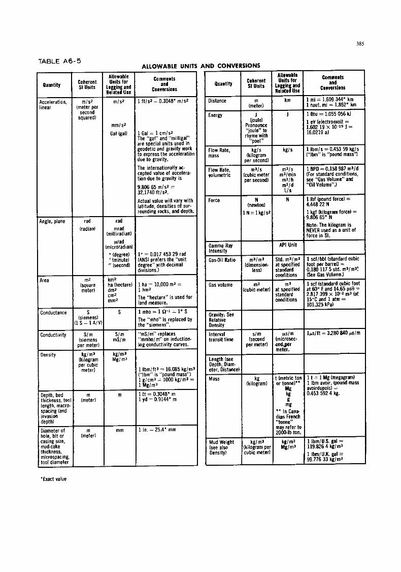
385
TABLE A 6 - 5 ALLOWABLE UNITS AND CONVERSIONS
Allowable Units for
Logging and Related Use
Comments and
Conversions
Allowable Units for
logging and Related Use
Comments and
Conversions
Coherent SI Units I
1 mi = 1.609 344’ km 1 naut. mi = 1.852’ km
1 f t /@ = 0.3048’ m/s* km
1 Btu = 1.055 056 k l 1 eV (electronvolt = 1.602 19 x 10-19 1 = 16.0219 al
I Energy (joule)
Pronounce “joule” to rhyme with
“OOOl”
mm/sZ
Gal (gal) 1 Gal = 1 cmls2 The “gal” and “milliga!” are special units used in geodetic and gravity work to express the acceleration due to gravity.
The internationally ac- cepted value of accelera- tion due to gravity is
~
1 lbmls = 0.453 59 kgls (“lbm” is “pound mass”)
Flow Rate, kg l s mass I (kilogram
oer second)
kgls
1 BPD = 0.158 987 m3ld (For standard conditions, see “Gas Volume” and “Oil Volume”.)
1 Ibf (pound force) = 4.448 22 N
m3/s m3lmin m3/h m3ld L l s N
Flow Rate, m3ls volumetric (cubic meter
per second) 9.806 65 mls2 = 32.1740 f t /s?
Actual value will vary with latitude, densities of sur- rounding rocks, and depth.
(newton) 1 k (kilogram force) = 9 . t 65’ N
1 N = 1 kg/sz rad
mrad (milliradian)
prad (microradian)
(degree) (minute)
It (second)
Note: The kilogram is NEVER used as a unit of force in SI.
API Unit Intensity
1” = 0.017 453 29 rad (ANSI prefers the,“unit degree” with decimal divisions.)
Std. m3lm3 at specified standard conditions
1 scf / bbl (standard cubic foot per barrel) = 0.180 117 5 std. m3lm3t (See Gas Volume.)
1 scf (standard cubic foot at 60” F and 14.65 psi) = 2.817 399 x 10-2 m3 (at 15°C and 1 atm = 101.325 kPa)
Gas-Oil Ratio m3/m3 (dimension-
less)
Gas volume m3 (cubic meter)
Gravity: See Relative Density
Interval s l m transit time (second
per meter)
Length (see Depth, Diam- eter, Distance)
km2 ha (hectare) dmz cm2 mmz
m3 at specified standard conditions
1 ha = 10,000 m2 = 1 hmz The “hectare“ is used for land measure.
1 mho = 1 52-1 = 1’ s The “mho” is replaced by the ”siemens”.
S
“mS/m” replaces “mmho/m” on induction- log conductivity curves.
~ s l m (microsec- andger meter.
l ps l f t = 3.280 840 pslm S/m mSlm
1 Ibm/ft3 = 16.085 kglm3 (“lbm” is “pound mass”) 1 g/cm3 = 1000 kg/m3 = 1 Mglms
1 f t = 0.3048’ m 1 yd = 0.9144’ m
1 t = 1 Mg (megagram) 1 Ibm avoir. (pound mass avoirdupois) = 0.453 592 4 kg.
t (metric to1 or tonne)’”
Mg kg g
mg ” In Cana- dian French “tonne” may refer ti 2000-lb ton
kglm3 Mglm3
m
~~
1 in. = 25.4’ mm mm
1 1bmlU.S. gal = 119.826 4 kglm3 1 1bmlU.K. gal = 99.776 33 kglms
Density) cubic meter1
’Exact value
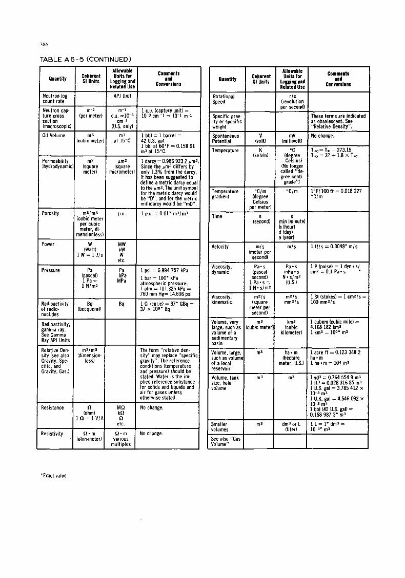
386
TABLE A 6 - 5 (CONTINUED 1
K (kelvin)
Coherent SI Units
“C Toc = TK - 273.15 (degree Celsius)
TVa = 32 + 1.8 x TOc
Allowable Units for
logging ant Related Use
~~
P a - s Pa. s (pascal mPa-s second) N - s/m2
1 Pass = (U.S.) 1 N - s l m 2
m2/s m2/s (square mm2/s
meter per second)
m3 km3 cubic meter) (cubic
kilometer)
m3 ha m (hectare
meter, U.S.)
Comments and
Conversions
1 P (poise) = 1 dyn s! cm2 = 0 . 1 Pa*s
1 St (stokes) = 1 cm2/s = 100 mm*/s
1 cubem (cubic mile) = 4.168 182 km3 1 km3 = log* m3
1 acre ft = 0.123 348 2 ha - m 1 ha m = 104 m3
~~~~
C o h e r e n t T i t s Allowable for I SI Units logging and
Related Use Conversions Quantity Quantity
Neutron Jog count rate
~~~
API Unit Rotational Speed (revolution
per second) + ~ ~
m-1 (per meter:
m-1
cm-1 (US. only)
C.U. =lo-3 1 C.U. (capture unit) = 10-3 cm -1 = 10-1 m-1
Neutron c a p ture cross section (macroscopic
O i l Volume
These terms are indicated as obsolescent. See “Relative Density”.
Specific grav i ty or specifii weight
Spontaneous Potential 7 j - T (mi I Iivo It) (vo It)
~
m3 (cubic mete1
m3 at 15°C
No change. 1 bbl = 1 barrel = 42 US. gal. 1 bbl at 60°F = 0.158 91 m3 at 15°C. Temperature
~
m2 (square meter)
Permeability (hydrody nami
Pm2 (square
micrometer1
1 darcy = 0.986 923 2 pm2 Since the pm* differs by only 1.3% from the darcy, it has been suggested to define a metric darcy equal to the @rnz.The unit symbol for the metric darcy would be “D”, and for the metric millidarcy would be “mD”.
1 p.u. = 0.01* m3/m3
(No longer called “de- gree centi-
grade”)
(degree Celsius
per meter)
Temperature gradient
l”F/lOO f t = 0.018 227 “C/m
Porosity ~~
m3/m3 (cubic mete
per cubic meter, di-
mensionless
p.u. Time
h (hour) d (day) a (year)
(meter per second)
Power w (Watt)
1 w = 1 J/ !
MW kW W
etc.
Velocity
Viscosity, dynamic Pressure Pa
(pascal) 1 Pa = 1 N/m2
Pa kPa
MPa
1 psi = 6.894 757 kPa 1 bar = 100’ kPa atmospheric pressure: 1 atm = 101.325 kPa = 760 mm Hg= 14.696 psi Viscosity,
kinematic Radioactivity of radio- nuclides
~
1 Ci (curie) = 37’ GBq = 37 x 109’ Bq
Volume, very large, such as volume of a sedimentary basin
Radioactivity, gamma ray. See Gamma Ray API Units
Relative Den- sity (see also Gravity, Spe- cific, and Gravity, Gas.)
m3/m3 (dimension-
less)
The term “relative den- sity” may replace “specific gravity”. The reference conditions (temperature and pressure) should be stated. Water is the im- plied reference substance for solids and liquids and air for gases unless otherwise stated.
Volume, large such as volum of a local reservoir
Volume, tank size, hole volume
m3
m 3 1 I 10-3 m3
1 yd3 = 0.764 554 9 m3 1 f t3 = 0.028 316 85 m3 1 US. gal = 3.785 412 x
lU.K. gal = 4.546 092 x
1 bbl (42 U.S. gal) = 0.158 987 3* m3
Resistance No change. (ohm)
etc. Smaller volumes
See also “Gas Volume”
Resistivity No change.
multiples
‘Exact value

387
TABLE A 6 - 6 ROUNDUP OF UNIT SYMBOLS FOR
UNITS WITH NAMES
Symbol
a, ha a atm A A b bar B, dB Bq cd c Ci "C d D eV F g Gal
h H HZ
J kg kn K Im
GY
Unit I Status
are, hectare year (annum) atmosphere ampere angstrom barn bar bel, decibel becquerel candela coulomb curie degree Celsius day darcy (metric) electronvol t farad gram gal gray hour henry hertz joule kilogram knot kelvin lumen
allowable allowable limited allowability base unit limited allowability limited allowability limited allowability allowable derived unit base unit derived unit limited allowability allowable allowable allowable allowable derived unit derived unit limited allowability derived unit allowable derived unit derived unit derived unit base unit limited allowability base unit derived unit
TABLE A6-7
Metricated values of some constants
Atmosphere: Density of dry air at 0°C and 1 atm: Molar gas constant, R: Avogadro constant, NA:
Velocity of light, c: Faraday constant, F: Permeability of free space, po: Standard acceleration due to gravity, g: Volume of 1 mol of ideal gas under standard conditions (at 15°C and 1 atm): Planck constant, h: Boltzmann constant, k: Electron rest mass, me: Proton rest mass,m,: Neutron rest mass, m,:
1 atm = 101.325 kPa 1.2929 kg/m3
R = 8.314.J/(mol.K) N, = 6.0220X mo1-I c = 299.792 46 Mm/s F = 96.484 kC/mol p o = 1.256 637 H/m
g = 9.806 65 m/s2 23.64 L
h = 6.626176X j s k = I.38054X j K-I m, = 9.10956~ kg m p = 1.67261 x kg m, = 1.67492X kg
Symbol
Ix L, 1, p m min mol N naut. mi. (no symbol) PS Pa r rad rd R
sr S t T
S
U
V W Wb Q 0
I
It
TABLE A64
SI prefixes
Unit
lux liter meter minute (time) mol newton nautical mile
parsec pascal revolution (as r/s) radian rad roentgen second (time) steradian siemens metric ton (tonne) tesla unified mass unit
(formerly amu) volt watt weber ohm degree (angle) minute (angle) second (angle)
status
derived unit allowable base unit allowable base unit derived unit limited allowability
allowable derived unit allowable supplementary unit limited allowability limited allowability base unit supplementary unit derived unit ? derived unit allowable
derived unit derived unit , derived unit derived unit allowable allowable allowable
Multipli- SI prefix SI prefix cation for unit for unit factor name symbol
10'8 hexa H 1015 penta P 10'2 tera T 109 gigs G 106 mega M 103 kilo k 102 hecto h 10 deca da 10-1 deci d 10-2 centi C
milli m 10-6 micro P 1 0 - ~ nano n 10-12 pic0 P 1 0 - l ~ femto f 10-18 atto a
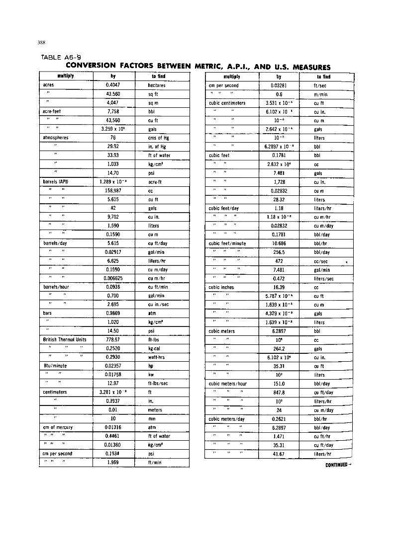
388
multiply
acres
TABLE A6-'9
by to find
0.4047 hectares
43,560 SQ f t
multiply I by to find
I
0.6 , * I , , I
cubic centimeters I 3.531 x I "
mfmin
cu f t
6.102 x lo-'
10-8
cu in.
cu m
I, ,I
barrels/hour
0.006625 cu m/hr
0.0936 cu f t /min cubic inches 16.39 cc
5.787 x 10⁻⁴
1.639 x
I, ,I
I , , I
cu f t
cu m
- 1.471 cu f t /hr
35.31 cu ft/day
41.67 liters/hr
,* I , ,I
* 1 , 9 , ,, - ,, , I 9 , cm per second
I , I, , I
0.1934 psi
1.969 ft/min
1 I acre-feet I 7,758 I bbl I I 'I I 43,560 I cu ft
1 I 2.642 x 10⁻⁴ I gals I " 3.259 x lo5 atmospheres cms of Hg
29.92 in. of Hg
33.93 f t of water
1.033
14.70
barrels (API) 1.289 x lo-' acre-ft
158,987
5.615 cu f t
I I ' 'I I 9,702 I cu in. I I 'I " I 1,590 I liters I I " " " I 0.02832 1 cu miday -1 I 'I " I 0.1590 I cu m I I " " I 0.1781 I bbl/day I I bar rebday I 5.615 I cu ft/day I I cubic feet/minute I 10.686 I bb l ih r I I " " I 0.02917 I gal/min I I " " " 1 256.5 I bbl/day I
I 1 6.625 liters/hr
0.1590 cu m/dav
,I I ,
I , I ,
I " " " I 472 I cc/sec * I I " " " I 7.481 I gal/min I
I 0.700 I gal/min I I * I , I
I " 'I I 2.695 I cu in./sec I I bars I Ci3869 I atm I I I' " I 4.329 x 7 gals I I I 1.020 I kg/cm* I I 1.639 x I liters I I I* I ,
I 'I I 14.50 I psi I I cubic meters I 6.2897 I bbl I
1 British Thermal Units I 778.57 I ft-lbs I 0.2520 kg-cal
0.2930 watt-hrs
Btulminute 0.02357
0.01758 kw 11 I ,
264.2 gals
I 12.97 1 ft-lbs/sec 1 I centimeters I 3.281 x lo-* I ft I
I 0.3937 1 in.
I 'I I 0.01 I meters I I 10 I mm
1 cm of mercury I 0.01316 I atm I I " " " I 0.4461 I f t of water I
I 0.01360 I kn/cmz I I 1, ,I 11
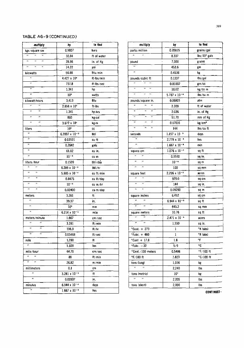
389
multiply
parts/million
by to find
0.05835 grains/gal
8.337 Ibs/lOn pals
multiply by
kgslsquare cm 0.9807
I " " I' 1 32.84 I ft of water i
to find
bars
I 28.96 I in. of Hg I 1 I , 9 , I , pound 7,000 grains 9 , I , I,
kilowatts
14.22 psi
56.88 Btu/min
4.427 x 10' ft-lbs/min
r
kilowatt-hours I, I ,
I ! 1 ,
I , ,, I , ,I
liters
103 watts
3,413 Btu
2.656 x 10' ft-lbs
1.341 hphrs
860 kgcal
3.672 x 10' kgm
103 cc
6.2897 x bbl
I* I,
9 9 I ,
!) I ,
I 7 I ,
I 9 I ,
seconds
2.309 ft of water
2.036 in. of Hg
51.70 mm of Hg
144 Ibs/cu ft
0.07031 kg/cma
1.157 x days
2.778 x lo- ' hrs
1.667 x l o - * min
9 , I ,
square inches , I I!
,I I,
square meters 1 1 I,
, I I ,
OCent. + 273
0.09290 sq m
6.452 sq cm
6.944 x sq f t
645.2 sq mm
10.76 sq ft
2.471 x l o - ' acres
1,550 sq in.
1 "K (abs)
meters/minute 1.667 crn/sec
3.281 ft /min
"Fahr. + 460 1 O R (abs)
T e n t + 17.8 1.8 "F
mile/hour I , I I
I , I ,
millimeters
minutes
44.70 cm/sec
88 ft/min
26.82 m/min
0.1 em
3.281 x f t
0.03937 in.
6.944 x l o - ' days
1.667 x hrs
"Cent./100 meters
"F/100 ft
tons (long)
tons (metric)
9 , I ,
,, I ,
tons (short)
0.5486 " F / l O O ft
1.823 "C/100 f t
1,016 kg 2,240 Ibs
103 kg 2,205 Ibs
2.000 Ibs
I 1 0.4536 I kg I I pounds/cubic f t I 0.1337 I Ibslgal I
I " 1 737.8 I ft-lbs/sec I I r , 9 , 1 0.01602 I gm/cc I ' I
I 1.341 I hp I ( 9 1 , I 16.02 I kg/cu m I r v
I , I ,, I 5.787 x l o - ' I Ibs/cu m I "
I poundsisquare in. I 0.06805 I atm I
I I S I 0.03531 I cu ft I I " I 0.2642 I gals
I 'I I 61.02 1 cu in. I I " I 10-3 I c u m I I " I 0.1550 I sq in. I I liters/hour I 0.1509 I bbl/day I I 10-4 I sq m I
I 6.289 x 1 bbl/hr I I , I I ,
I 5.885 x lo-' I cu ft/min I I ,I I , I square fee t I 2.296 x lo- ' I acres I I I' 'I I 0.8475 I cu ft/day I
cu m/hr
0.02400 cu m/day
meters 3.281
39.37 in.
103 mm
I '# 1 6.214 x l o - ' I mile I
I " 1 196.9 I f t /hr I I 'I I 0.05468 I ft/sec I I mile I 5,280 1 f t I I " I 1.609 I km I I "Fahr. -32 I 5/9 I "C
CONTINUED -

3 90
multiply by
grams 10-3
TABLE A6-9 (CONTINUED)
to find
kg
I multiply bv to find
I cubic meters/dav I 0.04167 I cu m/hr I
hofsepower
horseDower-hour
0.010 sq km
42.40 Btu/min
33,000 ft-lbs/rnin
550 ft-lbs/sec
1.014 metric hp
10.68 kg.cal/rnin
0.7457 kw
745.7 watts
2.544 Btu 0.3048 I , I , m/min
feethecond 30.48 cm/sec 9 , I I
foot-pounds
foot-pounds/rninute
foot-pounds/second
gallons (US)
I , I ,
# # I ,
,, ,I
,, I ,
18.29 m/mir:
1.285 x lo-: Btu
3.238 x 10⁻⁴ kgcal
3.030 x hP
1.818 x hP
2.260 x lo-' kw
1.356 x l O P kw
0.02381 bbl
3.785 cc
3.785 PI ,t l i ters
gallons (Imperial) 1.2009 gal (U.S.)
grainslgal 17.12 PPm
I 142.9 I, 11 Ibs/106 gals
I 0.3215 I oz I "
I " 1 86,400 1 sec I I feet I 30.48 1 crn I 1 grarns/cc I 62.43 I Ib/cu f t I
I 12 I in. I I ' ,* I 8.344 I Ibs/gal I I 1 0.3048 I meters I I I 0.03613 I Ibs/cu in. I I '
I feet of water 1 0.02950 I atm I I I grams/liter I 58.42 I grains/gal
I ', " I 0.8826 1 in. of Hg I I 1 hectares I 2.471 I acres
I " 1 0.03048 I kg/sq crn I I ', ', ' I I 62.43 I Ibsisq f t I I ,' I 0.4335 I psi I I feet/hour I 0.008467 1 cm/sec I
I 0.5080 I cm/sec I I 0.01667 I ft/sec I I 0.01829 I km/hr I
I " I 641.1 I kg.cal
I I 2.737 x loJ I kg-m I r r
I " I 0.7455 1 kw-hr . I I inches I 2.540 I cm I I " I 8.333 x I f t I
in. of mercury 0.03342
1.133 f t of water
0.03453 kg/sq cm
0.4912 psi
I in. of water I 0.002458 I atm I I 0.1337 I cu ft I I 0.07349 I in. of Hg I )' ' I "
I " I 231 I cu in. I I " " I 0.002538 I kg/crn* I I ') 'I I' I 0.03609 I psi I I kilograms I lo3 I gm I I 'I 1 2.205 I Ibs
I 1.102 x 1 tons (short) I I "
I " " I 34.286 I bbl lday I I kg-calories 1 3.986 I Btu I I " IS I 0.1337 I cu f t /min I I ' I " I 3,088 I ft-lbs I
I 192.5 I cu ft/day I I I , ,, I I 1.560 x I hphrs I ,' I '
I 3.785 1 l i ters/min I I I t I, I " I 427 I kg-meters I I 90.84 I liters/hr I 1 I* I, I I 1.163 x I kw-hrs I ) ' 'I
I grain (avoir~ I 0.06480 1 gm I I kg-calories/min 1 0.09358 1 hp I I " " " I 0.06977 1 kw I I k g s m b i c meter I I gm/cc I
I 0.01714 I gm/liter I I I ! I , I kgs/square cm I 0.9678 1 atm I I grams 1 15.432 I grains I CONTINUED -+

39 1
TABLE A 6 - 9 (CONTINUED)
I multiply I by I to find I multiolv 1 bv 1 to find I I viscosity, Ib-sec/sq in. I 6.895 x lo6 I viscosity, cp I I watts I low3 I kw
I viscosity, Ib-sec/sqft I 4.78 x 101 I viscosity, cp I I watt-hours I 3.413 I Btu I I viscosity, centistokes 1 density 1 viscosity, cp 1 1 watts I 0.05688 I Btu/min I I 1.341 x I I hp-hrs
I " I 44.27 1 ft-lbs/min I I " I 0.7378 I ft-lbS/SEC I I " I ' I 367.2 I kg-m I I 'I I 1.341 x I hp I I )' I' I I kw-hrs I I " I 0.01433 1 kg-cal/min I
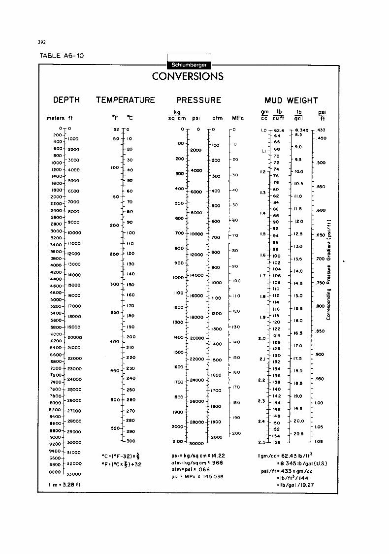
392
TABLE A6-10
32
5 0
loo
I 50 --
200
250
300
350
4 0 0
450
500--
550:-
CONVERSIONS
-0
- - 10
-- 20
_- 30
-- 4 0
-- 50
-- 6 0
-- 70
- -
- ao
-90
-- 100
-- 110
- - 120
_- 130
- 140
-- I 5 0
-- 160
- - 170
- _
-_ --
iao
- 190
-- 200 -- --210
_- 220
-: 230
-- 240
-- 250
260
-- 270
- 280
290
-L 300
-
DEPTH
1.0
1.1
1.2 -
1.3 -
--
1.5 1- --
_- 1.6 --
-- --
1.7 -- -- --
1.a -- 1- --
1.9 -- -- -- --
2.0-
_-
meters f t
O T 0 - 62.4 -- 6 4 - - 6 6
-- 6a -- 70
-- 72
-- 74
-- 76
_- 78
-- ao -- 82
-- 84
-- 86
I- 8a 9 0
_- 92
94 96
9a
100
102 104
106
I08
110
112
114
I16
I 18 120
122
124
--126 128
- -
--
- --
- - - -
-
60,j 6 200 20000
- 8.345 - ,433 -- 8.5 - - ,450
_ - 9.0 -
-- 9-5 - ,500
- 10.0 -
:-lo-’ - ,550
11.0 -
- - l l . 5 - ,600 - c - 12.0 - \ .-
--12.5 - .650 2 - c C 0
0 .- - 13.0 - e
3
t
- 13.5 - .700
.)
n - 14.0 -
--l4.5 - . 7 5 0 n
rn c .- --15.0 -
GOO--
800
1000-:
I200
1400-’
1600-: 1800--
2000--
2200--
2400--
2600--
2 m - -
3000--
3200--
JBOO--
4000--
4200-- 4400-
4600--
4800--
sow-. 5 200 -- 5400-
5600-.
5800--
TEMPERATURE
2000
3000
-- 4000
5000
6000
7000
8000
9000
10000
3400--11000
-.
~ o o - - 1 2 0 0 0
13000
14000
l5000
16000
I7000
- I8000
19000
OF “C
_-
1- -
0 16.0 - 16.5 1 ‘850
-17.0 -
PRESSURE kg
sq cm psi atm MPa
r
I800
1900
2000
2100
6400--
6600--
6800-.
7000--
7200-’
7400-:
7600--
7800-’
Booo 8200--
8400--
8600--
8800--
9OOo--
9 200
9600-
9800 -- loooo--
26000
28000
30000
21000
- 22000
23000
24000
25000
-26000
27000
28000
29000
-- 3 ~ 0 0 0
31000
3 2 000
33000
I700
I800
I900
2000
- ,900
- 950
- 1.00
- 1.05
r 1.08
ps i= kg /sqcrnx14 .22 atrn= kg/sq cm X .968 atm- psi X ,068 psi = MPa x 145038
0
10
20
30
40
50
6 0
70
80
90
100
I I0
120
I3 0
140
150
160
170
180
190
200
MUD WEIGHT 0 2 Ib Ib psi cc c u t qol T
2.3
2.4 20.0
154
I gm/cc = 62.43 I b /f 1’ = 8 . 3 4 5 Ib/gal (U.S.)
psi/f t = . 4 3 3 x grn /cc = Ib/ft’/ 144 = Ib /ga l /19.27
8
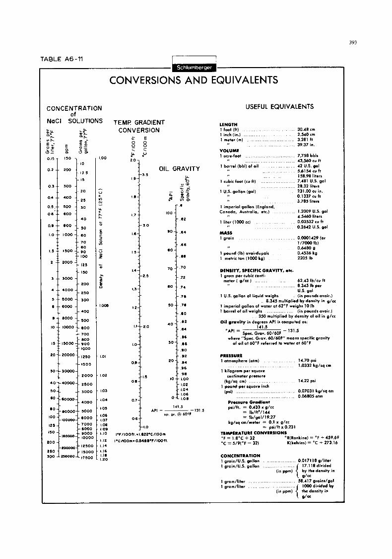
TABLE A6-11
CONVERSIONS AND EQUIVALENTS
0.15 - I 5 0 7
0.2 -- 200 -
0 . 3 - - 300 -
0.4 -- 400 -
0.5.-- 500
0.6 -- 600 -
0.8 -- 800 - + 7
CONCENTRATION of
NaCl SOLUTIONS
- 10 - 12.5
-- I 5
_- 2 0
25
-- 30
_- 40
5o
l o - -
17- -
I 6 - -
15 -
14-
13-
12--
I O -
09-
0 8 -
07 -
. - 3 0
1-2 5
11--20
- - I 5
1
2 0 20000 1250
1500
2 0 0 0
4 0 40000 2500 -i--: 5 0 3000
- 100 -
so--
_ - 80 -
70
60 --
50
4 0
30:-
2 0 : -
10
0 %
I25
150
200
250 1sooo
.6
.- ,132
.64
.68
.- .68
_- .72
74
_- . re
-- .?I
- - .a0
l- .02
_ - .84
_- .86
.88
.- .so
.- .92
94
- - 96
_ - 98 -- 1.00
.- 1.04
.- 1.06 1.08
:- 1.02
.oo
- 2
rY U
L
L
L
L
0
3
3
4 - 3
L 0
21 c - E l .mu
1.01
1.02
I .03
1.04
to5
I .06 1.07 1.08 1.09 1.10
1.12 1.14 1.16 1.18 1.20
3
4
5
8
8
10
TEMP GRADIENT CONVERSION
.- 150
-- moo - - - 200
- 250 -- 4000 - -- 5000 -- 300
_- 400 -- 6000 -
-- 8000 - 5oo
- - 10000 -- 600
OIL GRAVITY
141.5 API = -131.5
sp. gr. @ 60°F
0.6i 1.0
I.F1100ft. =I.022.C1100m
1% AOOm - Ob488.FI 1 0 0 11.
USEFUL EQUIVALENTS
LENGTH 1 foot (ft) 30.48 cm 1 inch (in.) 2.540 cm 1 meter (m) 3.281 ft
39.37 in. VOLUME 1 acre-foot 7,758 bbls
43,560 cu f t 1 barrel (bbl) of oil 42 US. gal
54154 cu ft 158.98 liters 7.481 US. gal 28.32 liters 231.00 cu in. 0.1 337 cu ft 3.785 liters
1.2009 US. gal 4.5460 liters 0.03532 cu ft 0.2642 US. gal
1 cubic foot (cu ft)
1 US. gallon (gal)
1 imperial gallon (England, Canada, Australia, etc.)
1 liter (1OOO cc)
MASS 1 grain O.OOO1429 (or
1 /7o00 Ib) 0.6480 9 0.4536 kg 1 pound (Ib) avoirdupois
1 metric tan (lo00 kg) 2205 Ib
DENSITY, SPEClflC GRAVITY, ok. 1 gram per cubic centi-
meter ( p/cc ) 62.43 Ib/cu ft 8 345 Ib per
(in pounds avoir.) us gal
1 U S. gallon of liquid weighs
1 imperial gallon of water at 62°F weighs 10 Ib 1 barrel of oil weighs
Oil gravity in degrees API is computed as:
8.345 multiplied by density in g/cc
(in pounds ovoir.) 350 multiplied by density of oil in g/cc
141.5 "API = Spec, Grav. 60160F - 1313 where "Spec. Grav. 60/60F" means specific gravity
of oil at 60°F referred to water at 60°F
PRESSURE 1 atmosphere (atm) 14.70 psi
1 kilogram per square centimeter pressure
1 pound per square inch
1.0332 kg/sq cm
(kglsq cm) 14.22 psi
(psi) 0.07031 kg/sq cm 0.06805 atm
Prorsuro Gradiont psi/ft. = 0.433 x g/cc
= lb/ft5/144 = lb/ga1/19.27
kg/sq cm/meter = 0.1 x g/cc = psi/ft x 0.231
TEMPERATURE CONVERSION! "F=l .BoC+32 "C = 5/9("F - 32)
R(Rankine) = O F + 459.69 K(kelvins) = "C + 273.16
CONCENTRATION 1 grain/U.S. gallon .................... 0,0171 18 g/liter 1 grain/U.S. gallon ...................... 17.1 18 divided
1 gram/liter ................................ 58.417 grains/gal 1 grom/liter ........................... lo00 divided by
393

This Page Intentionally Left Blank
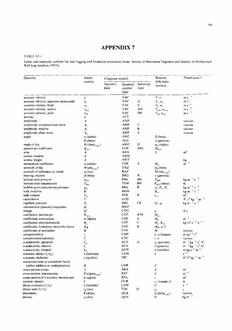
395
APPENDIX 7 TABLE A7-1
Letter and computer symbols for well logging and formation evaluation (from: Society of Petroleum Engineers and Society of Professional Well Log Analysts (1975))
Quantity Letter. Computer symbol Reserve Dimensions * symbol SPE letter
Operator Quantity Subscript symbols field symbol field
field
acoustic velocity acoustic velocity, apparent (measured) acoustic velocity, fluid acoustic velocity, matrix acoustic velocity, shale activity amplitude amplitude, compressional wave amplitude, relative amplitude, shear wave angle
angle of dip anisotropy coefficient area atomic number atomic weight attenuation coefficient azimuth of dip azimuth of reference on sonde bearing, relative bottom-hole pressure bottom-hole temperature bubble-point (saturation) pressure bulk modulus bulk volume capacitance capillary pressure cementation (porosity) exponent charge coefficient, anisotropy coefficient, attenuation coefficient, electrochemical coefficient, formation resistivity factor coefficient or multiplier compressibility concentration (salinity) conductivity, apparent conductivity, electric conductivity, thermal constant, decay ( constant, dielectric correction term or correction factor
(either additive or multiplicative) cross-section (area) cross-section, macroscopic cross-section of a nucleus, microscopic current, electric decay constant ( I /T , , ) decay time ( I / h ) decrement density
1)
'?,
ur urn d
a A
h
A, A , A, a (alpha) 0 (theta) 0 (theta,,,) K,", A Z A a (alpha) aJ ( P h L P ) P (mu) P (beta) P h h
Tb h
P h K
C
rn
'h
pc
Q K a n , a (alpha) K , KR K
C
C
h (lambda) c (epsilon)
C
c,
k h
B A
Z (sigma,,,) u (sigma) I h (lambda) Td (tau) 6 (delta) P (rho)
VAC VAC VAC VAC VAC ACT AMP AMP AMP AMP ANG AGL ANG COE A RA AN M AWT COE DAZ RAZ BRG PRS TEM PRS BKM VOL
ECQ PRS MXP C H G COE COE COE COE COE CMP CNC ECN ECN HCN LAM DIC
COR ARA XST XNL CUR LAM TIM DCR DEN
A F MA SH
C R S
D AN I
A
R BH BH B
B
C P
AN1 A C R
A
D
m s - ' m s - ' m s - ' m s - ' m s - '
various various various various
m2
kg m - ' s - '
K kg m - ' sC2 kg m - ' s - ~ m3 A' s 4 kg-l m - 2 kg m - ' s - '
A s
m2 m - ' m2
S - I
A
S
various kg m-'
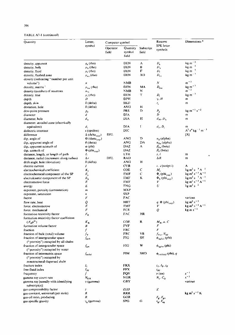
396
TABLE A7-1 (continued)
Quantity Reserve Dimensions * Letter, Computer symbol symbol -SPE letter
Operator Quantity Subscript symbols field symbol field
field
density, apparent density, bulk density, fluid density, flushed zone density (indicating “number per unit
density, matrix I
density (number) of neutrons density, true depth depth, skin deviation, hole dew-point pressure diameter diameter, hole diameter, invaded zone (electrically
equivalent) dielectric constant difference dip, angle of dip, apparent angle of dip, apparent azimuth of dip, azimuth of distance, length, or length of path distance, radial (increment along radius) drift angle, hole (deviation) electric current electrochemical coefficient electrochemical component of the SP electrokinetic component of the SP electromotive force energy exponent, porosity (cementation) exponent, saturation factor flow rate, heat force, electromotive force, mechanical formation resistivity factor formation resistivity factor coefficient
formation volume factor fraction fraction of bulk (total) volume fraction of intergranular space
(‘‘porosity”) occupied by all shales fraction of intergranular space
(“porosity”) occupied by water fraction of intermatrix space
(“porosity”) occupied by nonstructural dispersed shale
volume”)
( FR+m
fracture index free fluid index frequency gamma ray count rate gamma ray [usually with identifying
gas compressibility factor gas constant, universal (per mole) gas-oil ratio, producing gas specific gravity
subscript(s)]
n
Pma (rho)
Pt (rho) n N
D 6 (delta) 6 (delta)
d Pd
d h
di c (epsilon) A (delta,,,) DEL 0 (theta,,,) 0 (theta) + (Phi) @ (Phicap) L A r DEL 6 (delta) I
Kc Ec E k
E E m
n F
E F
Q
F R
KR
f f v
B
fdsh
f*w
f*shd
DEN DEN DEN DEN
NMB DEN NMB DEN DPH SKD ANG PRS DIA DIA
DIA DIC
ANG ANG DAZ DAZ LTH RAD ANG CUR COE EMF EMF EMF ENG MXP SXP FAC HRT EMF FCE FAC
COE FVF FRC FRC FIG
FIG
FIM
FRX FFX FQN NGR GRY
ZED RRR GOR SPG
A B F xo
MA N T
H D
H
I
D DA A
H
C C K
HR
R
VB SH
W
SHD
G
kg m - 3 kg m - 3 kg m-’ kg m - 3
m - 3 kg m - 3 m-’ kg m - 3 m m
kg m - ’ m m
m m
b
A kg m2 s C 3 A - ’ kg m2 s C 3 A - ’ kg m2 s C 3 A - ’ kg m2 sC3 A - ’ kg m2 sC2
various kg m2 s C 3 kg m2 s C 3 A - l kg m sC2
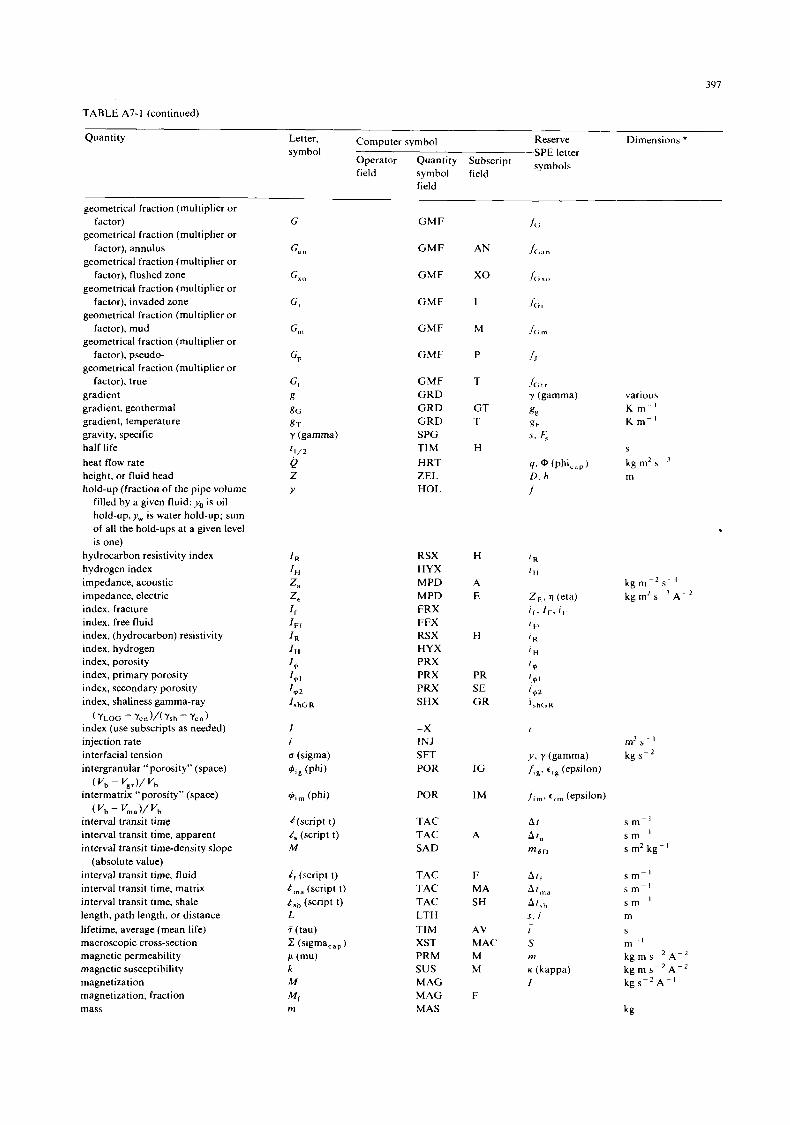
397
TABLE A7-1 (continued)
Quantity Letter, Computer symbol Reserve Dimensions *
Operator Quantity Subscript symbols field symbol field
symbol -SPE letter
field
geometrical fraction (multiplier or
geometrical fraction (multiplier or
geometrical fraction (multiplier or
geometrical fraction (multiplier or
geometrical fraction (multiplier or
geometrical fraction (multiplier or
geometrical fraction (multiplier or
gradient gradient, geothermal gradient, temperature gravity, specific half life heat flow rate height, or fluid head hold-up (fraction of the pipe volume
filled by a given fluid: yo is oil hold-up,y, is water hold-up; sum of all the hold-ups at a given level is one)
factor)
factor), annulus
factor), flushed zone
factor), invaded zone
factor), mud
factor), pseudo-
factor), true
hydrocarbon resistivity index hydrogen index impedance, acoustic impedance, electric index, fracture index, free fluid index, (hydrocarbon) resistivity index, hydrogen index, porosity index, primary porosity index, secondary porosity index, shaliness gamma-ray
index (use subscripts as needed) injection rate interfacial tension intergranular "porosity" (space)
intermatrix "porosity" (space)
interval transit time interval transit time, apparent interval transit time-density slope
interval transit time, fluid interval transit time, matrix interval transit time, shale length, path length, or distance lifetime, average (mean life) macroscopic cross-section magnetic permeability magnetic susceptibility magnetization magnetization, fraction mass
(?LOG - ycn)/(Ysh - Yen)
( 'b - 'gr )/ 'b
( 'b - 'ma )/ 'b
(absolute value)
G M F
G M F
GMF
G M F
G M F
G M F
G M F G R D G R D G R D SPG TIM HRT ZEL HOL
RSX HY X MPD MPD FRX FFX RSX HY X PRX PRX PRX SHX
-X INJ SFT POR
POR
TAC TAC S A D
TAC TAC TAC LTH TIM XST PRM sus MAG MAG MAS
AN
XO
I
M
P
T
G T T
H
H
A E
H
PR SE GR
IG
IM
A
F MA SH
AV MAC M M
F
f< i
fl
kg m - ' s - '
k g m ' s - ' A
m3 s - ' kg s - *
s m - ' s m - ' s m2 kg- '
s m - ' s m - ' s m - ' m
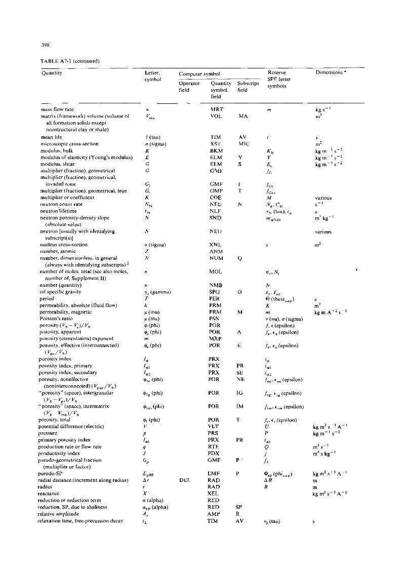
398
TABLE A7-I (continued)
Quantity Dimensions * Letter, Computer symbol Reserve symbol SPE letter
Operator Quantity Subscript symbols field symbol field
field
mass flow rate W
matrix (framework) volume (volume of Vm il all formation solids except nonstructural clay or shale)
mean life 7 (tau) microscopic cross-section u (sigma) modulus, bulk K modulus of elasticity (Young’s modulus) E modulus, shear multiplier (fraction), geometrical multiplier (fraction). geometrical,
multiplier (fraction), geometrical. true multiplier or coefficient neutron count rate neutron ‘li fetime neutron porosity-density slope
(absolute value) neutron [usually with identifying
subscript(s)] nucleus cross-section number, atomic number. dimensionless, in general
(always with identifying subscripts) ’ number of moles, total (see also moles,
number of, Supplement 11) number (quantity) oil specific gravity period permeability. absolute (fluid flow) permeability, magnetic Poisson’s ratio porosity ( Vh - y ) / Vb porosity, apparent porosity (cementation) exponent porosity, effective (interconnected)
porosity index porosity index, primary porosity index, secondary porosity, noneffective
“porosity” (space), intergranular
“porosity” (space), intermatrix
porosity. total potential difference (electric) pressure primary porosity index production rate or flow rate productivity index pseudo-geometrical fraction
pseudo-SP radial distance (increment along radius) radius reactance reduction or reduction term reduction, SP. due to shaliness relative amplitude relaxation time, free-precession decay
invaded zone
( vpe / ‘h)
(noninterconnected) ( VPne/ Vh)
( ‘h - ‘gr )/ ‘h
( Vb - ’ma ) / V b
(multiplier or factor)
MRT VOL
TIM XST BKM ELM ELM GMF
GMF GMF COE NEU NLF SN D
N EU
XNL ANM NUM
MOL
NMB SPG PER PRM PRM PSN POR POR MXP POR
PRX PRX PRX POR
POR
POR
POR VLT PRS PRX RTE PDX GMF
EMF DEL RAD
RAD XEL RED RED AMP TIM
MA
AV MIC
Y S
I T
N
Q
0
M
A
E
PR SE N E
IG
IM
T
PR
P .
P
SP R AV
111 k g s - ’ m3
t
S
t”
N
0 (theta,,,) K m Y (nu), u (sigma) J , z (epsilon) J,, (epsilon)
$0. e0
J,. z e (epsilon)
J,. z (epsilon) (I
P
I,,
Q i J J
r2 (tau)
various s-I S
m3 kg-’
various
m2
S
m2 kg m A - 2 s C 2
kg m2 sC3 A - ’ m m kg m2 sC3 A-’
S
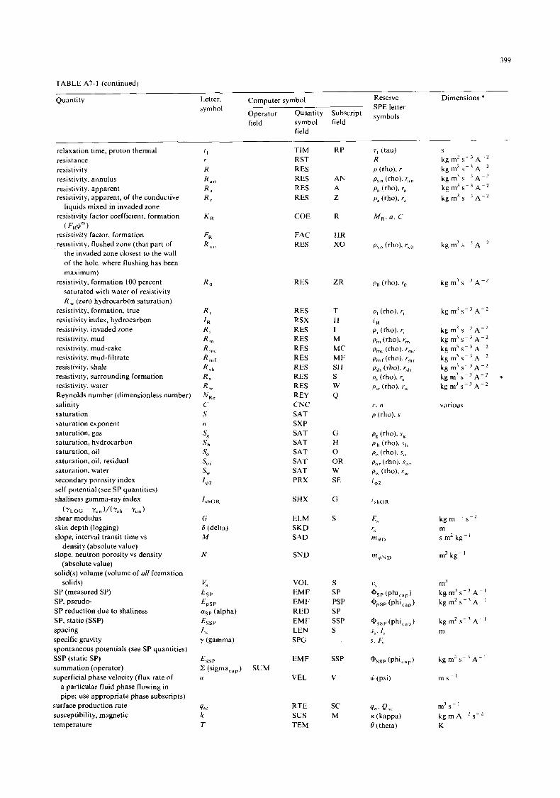
399
TABLE A7-1 (continued)
Dimensions * Quantity Letter, symbol
Computer symbol Reserve
Operator Quantity Subscript symbols field symbol field
SPE letter
field
TIM RP RST RES RES AN RES A RES Z
relaxation time, proton thermal resistance resistivity resistivity. annulus resistivity, apparent resistivity, apparent, of the conductive
resistivity factor coefficient, formation
resistivity factor. formation resistivity, flushed zone (that part of
liquids mixed in invaded zone
( FR@m )
the invaded zone closest to the wall of the hole, where flushing ha5 been maximum)
saturated with water of resistivity R , (zero hydrocarbon saturation)
resistivity, formation 100 percent
resistivity, formation. true resistivity index, hydrocarbon resistivity, invaded zone resistivity, mud resistivity, mud-cake resistivity, mud-filtrate resistivity. shale resistivity, surrounding formation resistivity. water Reynolds number (dimensionless number) salinity saturation saturation exponent saturation, gas saturation, hydrocarbon saturation, oil saturation, oil. residual saturation, water secondary porosity index
COE R
FAC HR RES xo kg rn’ s - A-’
R, , RES ZR
RES T RSX H RES I RES M RES MC RES M F RES SH RES S RES W
REY Q CNC SAT SXP SAT G SAT H SAT 0 SAT OR SAT W PRX SE
N R , C various
self potential (see SP quantities) shaliness gamma-ray index
shear modulus skin depth (logging) slope, interval transit time vs
density (absolute value) slope, neutron porosity vs density
(absolute value) solid(s) volume (volume of oll forma
solids) SP (measured SP) SP, pseudo-
( YLOC - Ycn )/( Ysh - yen)
SHX G ‘*hGR
k g m - ’ sC2 m s m2 kg-
m3 kg-’
G S (delta) M
ELM S SKD SAD
N SND
ition Y Es P
E p S P
asp (alpha) E S S P
VOL S EMF SP EMF RED EMF LEN SPG
PSP SP SSP S
SP reduction due to shaliness SP, static (SSP) spacing specific gravity spontaneous potentials (see SP quantities) SSP (static SP) summation (operator) superficial phase velocity (flux rate of
a particular fluid phase flowing in pipe; use appropriate phase subscripts)
surface production rate susceptibility, magnetic temperature
E S S P
Z (sigma,,,) U
EMF
VEL SUM
SSP
V m 5 - l
RTE sus TEM
sc M
4-c k T
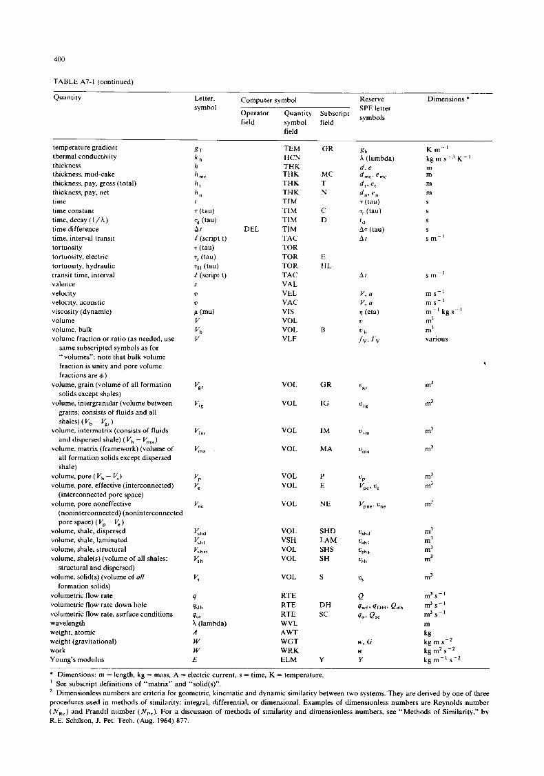
400
TABLE A7-1 (continued)
Quantity Letter, Computer symbol Reserve Dimensions * symbol SPE letter Operator Quantity Subscript
field symbol field symbols
field
temperature gradient thermal conductivity thickness thickness, mud-cake thickness, pay, gross (total) thickness, pay, net time time constant time, decay ( I / X ) time difference time, interval transit tortuosity tortuosity, electric tortuosity, hydraulic transit time. interval valence velocity velocity. acoustic viscosity (dynamic) volume volume, bulk volume fraction or ratio (as needed, use
same subscripted symbols as for “ volumes”; note that bulk volume fraction is unity and pore volume fractions are +)
volume, grain (volume of all formation solids except shales)
volume, intergranular (volume between grains; consists of fluids and all shales) (V, - 5,)
volume, intermatrix (consists of fluids and dispersed shale) ( Vb - Vma)
volume, matrix (framework) (volume of all formation solids except dispersed shale)
volume, pore ( Vb - V , ) volume, pore, effective (interconnected)
(interconnected pore space) volume, pore noneffective
(noninterconnected) (noninterconnected pore space) ( Vp - V, )
volume, shale, dispersed volume, shale, laminated volume, shale, structural volume, shale(s) (volume of all shales:
structural and dispersed) volume, solid(s) (volume of a//
formation solids) volumetric flow rate volumetric flow rate down hole volumetric flow rate, surface conditions wavelength weight, atomic weight (gravitational) work Young’s modulus
TEM HCN THK THK THK THK TIM TIM TIM
DEL TIM TAC TOR TOR TOR TAC VAL VEL VAC VIS VOL VOL VLF
G R K m - ’ k g m s - ’ K - ’ m m m m S
S
S
S
s m - ‘
MC T N
C D
E HL
s m - ‘ A I
m s - ‘ m s - ’ m - ’ k g s - ’ m3 m3 various
B
VOL G R
IG
m3
m3 VOL V i g
VOL m3
m3
Y m IM
MA Vm a VOL
VP K
VOL VOL
P E
m3 m3
m3 VOL N E
m3 m3 m3 m3
VOL VSH VOL VOL
SHD LAM SHS SH
hd
‘sbl
%hs
% h
m3 K VOL S
RTE RTE RTE WVL AWT WGT WRK ELM
4
4sc X (lambda) A W W E
9 d h D H sc
H., G
Y W
Y
* Dimensions: m = length, kg = mass, A = electric current, s = time, K = temperature. ’ See subscript definitions of “matrix” and “solid(s)”. ’ Dimensionless numbers are criteria for geometric, kinematic and dynamic similarity between two systems. They are derived by one of three procedures used in methods of similarity: integral, differential, or dimensional. Examples of dimensionless numbers are Reynolds number ( N R e ) and Prandtl number ( N p , ) . For a discussion of methods of similarity and dimensionless numbers, see “Methods of Similaritv.” bv R.E. Schilson, J. Pet. Tech. (Aug. 1964) 877.
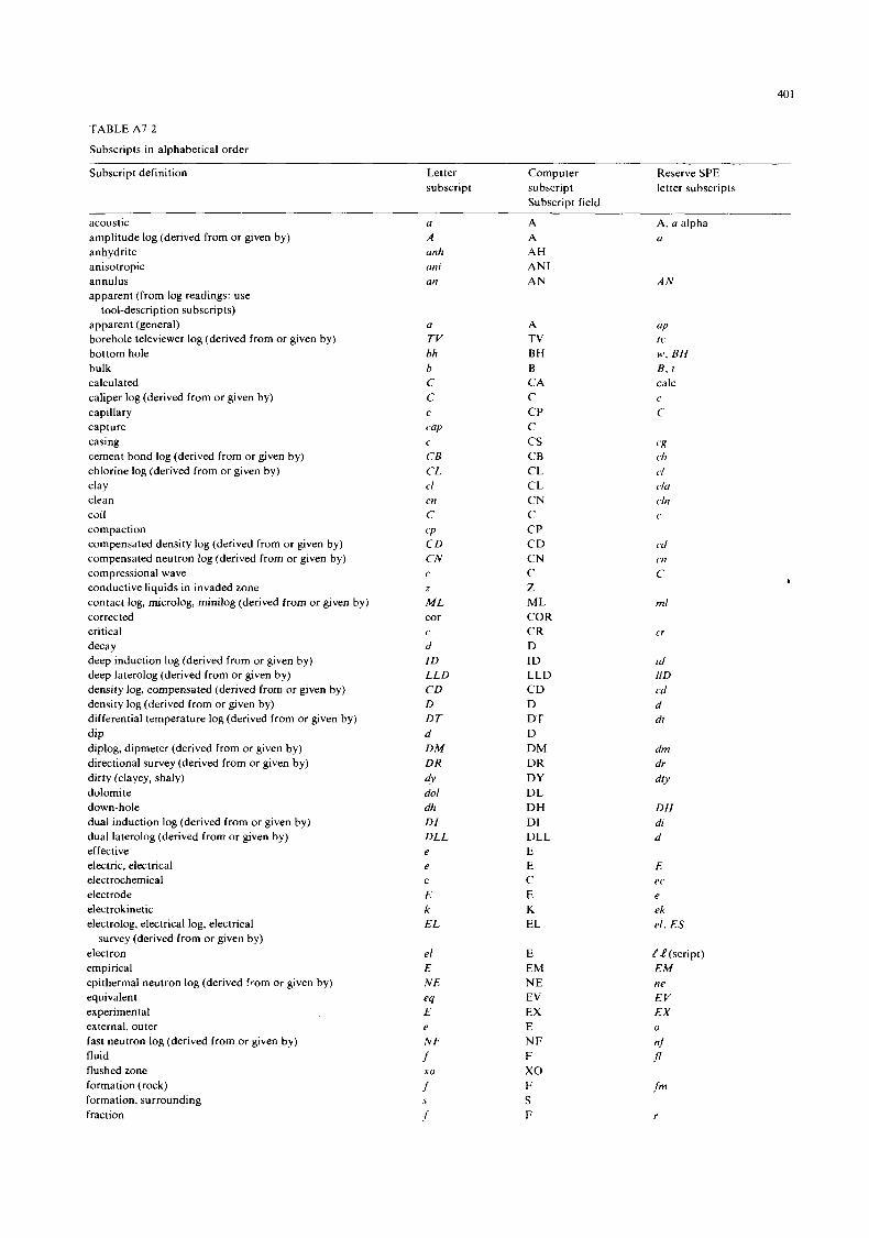
40 1
TABLE Al-2
Subscripts in alphabetical order
Subscript definition Letter Computer Reserve SPE subscript subscript letter subscripts
Subscript field
acoustic amplitude log (derived from or given by) anhydrite anisotropic annulus apparent (from log readings: use
tool-description subscripts) apparent (general) borehole televiewer log (derived from or given by) bottom hole bulk calculated caliper log (derived from or given by) capillary capture casing cement bond log (derived from or given by) chlorine log (derived from or given by) clay clean cail compaction compensated density log (derived from or given by) compensated neutron log (derived from or given by) compressional wave conductive liquids in invaded zone contact log, microlog, minilog (derived from or given by) corrected critical decay deep induction log (derived from or given by) deep laterolog (derived from or given by) density log, compensated (derived from or given by) density log (derived from or given by) differential temperature log (derived from or given by) dip diplog, dipmeter (derived from or given by) directional survey (derived from or given by) dirty (clayey, shaly) dolomite down-hole dual induction log (derived from or given by) dual laterolog (derived from or given by) effective electric, electrical electrochemical electrode electrokinetic electrolog, electrical log, electrical
electron empirical epithermal neutron log (derived from or given by) equivalent experimental external, outer fast neutron log (derived from or given by) fluid flushed zone formation (rock) formation. surrounding fraction
survey (derived from or given by)
U
A unh uni an
U
TV hh b C C C
cup
C B C L cl cn C
CP
CD C N
C
C
z
M L cor
d I D LLD CD D DT d D M DR
dY do1 dh DI DLL e e
E k EL
el E N E
eq E e N F
C
C
f
f
f
xo
r
A A AH AN1 AN
A TV BH B CA C C P C cs CB CL CL CN C C P C D CN C Z ML COR CR D I D LLD C D D DT D DM DR DY DL D H DI DLL E E C E K EL
E EM N E EV EX E N F F xo F S F
A. u alpha U
AN
UP
10
w . BH B , t calc
C c
“K ch
i.1 ciu (.in i’
cd cn C
mi
cr
id llD cd d dt
dm dr
dfY
DH di d
E ec e ek
el, ES
t4? (script) EM ne EV EX 0
nf
fm
r
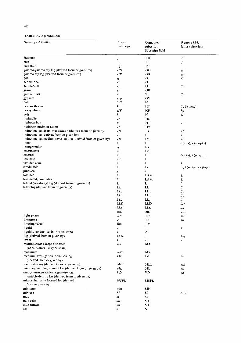
402
TABLE A7-2 (continued)
Subscript definition Letter Computer Reserve SPE subscript subscript letter subscripts
Subscript field
fracture free free fluid gamma-gamma ray log (derived from or given by) gamma ray log (derived from or given by) gas geometrical geothermal grain gross (total) gypsum half heat or thermal heavy phase hole hydraylic hydrocarbon hydrogen nuclei or atoms induction log. deep investigation (derived from or given by) induction log (derived from or given by) induction log, medium investigation (derived from or given by) inner intergranular intermatrix internal intrinsic invaded zone irreducible junction laminar laminated, lamination lateral (resistivity) log (derived from or given by) laterolog (derived from or given by)
light phase limestone limiting value liquid liquids, conductive, in invaded zone log (derived from or given by) lower matrix [solids except dispersed
(nonstructural) clay or shale] maximum medium investigation induction log
microlaterolog (derived from or gven by) microlog, minilog, contact log (derived from or given by) micro-seismogram log, signature log,
microspherically focused log (derived
minimum mixture mud mud cake mud filtrate net
(derived from or given by)
variable density log (derived from or given by)
from or given by)
J
FJ
F
GG G R
R G G gr
WP
h H P h H h H ID I IM i
' g im i int i i
.i I I L L L
t
1 /2
LL3 LL, LLR LLD LLS etc. LP Is lim L
LOG I ma
max IM
MLL M L VD
MSFL
min M m mc
mf
z
n
FR F FF GG G R G G GT GR T GY H HT HP H HL H HY ID I IM I IG IM I I I IR J LAM LAM L LL
LL3 LL, LLR LLD LLS etc. LP LS LM L 2 L L MA
MX IM
MLL ML V D
MSFL
MN M M MC MF N
F
f
m R' G
T
T
T , 6' (theta)
H hP
H
id
i im (iota), i (script i) 1
i (iota), 't (script i)
I ir, .J (script i), L (iota)
*
I
im
mll ml od
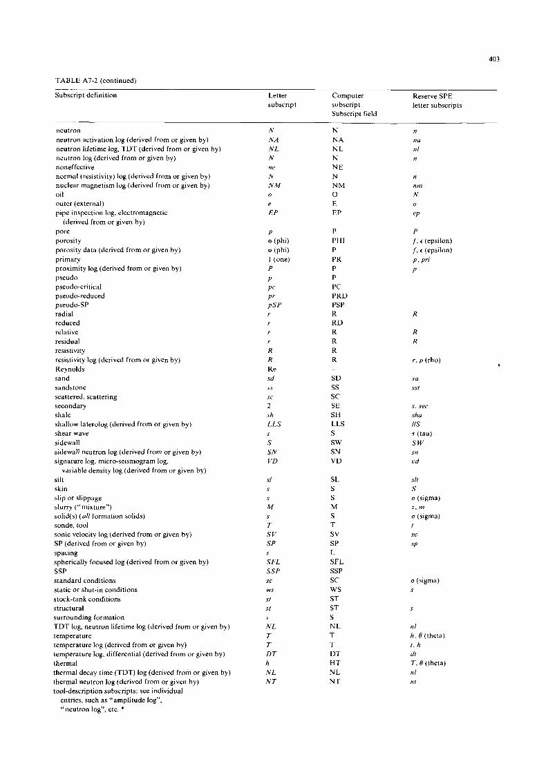
403
TABLE A7-2 (continued)
Subscript definition Letter Computer subscript subscript
Subscript field
neutron neutron activation log (derived from or given by) neutron lifetime log, T D T (derived from or given by) neutron log (derived from or given by) noneffective normal (resistivity) log (derived from or given by) nuclear magnetism log (derived from or given by) oi I outer (external) pipe inspection log, electromagnetic
pore porosity porosity data (derived from or given by) primary proximity log (derived from or given by) pseudo pseudo-critical pseudo-reduced pseudo-SP radial reduced relative residual resistivity resistivity log (derived from or given by) Reynolds sand sandstone scattered, scattering secondary shale shallow laterolog (derived from or given by) shear wave sidewall sidewall neutron log (derived from or given by) signature log, micro-seismogram log,
silt skin slip or slippage slurry (“mixture”) solid(s) (al l formation solids) sonde, tool sonic velocity log (derived from or given by) SP (derived from or given by) spacing spherically focused log (derived from or given by) SSP standard conditions static or shut-in conditions stock-tank conditions structural surrounding formation T D T log, neutron lifetime log (derived from or given by) temperature temperature log (derived from or given by) temperature log, differential (derived from or given by) thermal thermal decay time (TDT) log (derived from or given by) thermal neutron log (derived from or given by) tool-description subscripts: see individual
(derived from or given by)
variable density log (derived from or given by)
entries, such as “amplitude log”, “neutron log”, etc. *
N NA N L N ne N NM 0
e E P
P qJ (Phi) $J (phi) 1 (one) P
P P“ P‘
r r r r R R Re sd
PSP
ss sc 2 sh LLS
S SN V D
sl
S
S
S
M
T sv SP
SFL SSP
S
S
sc ws
st S t
S
N L T T D T h N L N T
N NA NL N N E N NM 0 E EP
P PHI P PR P P PC PRD PSP R R D R R R R
SD ss sc SE SH LLS S sw SN VD
SL S S M S T sv SP L SFL SSP sc ws ST ST S NL T T DT H T NL N T
-
~~~
Reserve SPE letter subscripts
-
n
nu nl n
n nm N 0
eP
P /, c (epsilon) /, c (epsilon) P . Pr‘ P
R
R R
r . p (rho)
sa sst
s. sec
sha 11s r (tau) sw sn vd
slr S a (sigma) z. m a (sigma) t St’
S P
a (sigma) S
S
n l h . 8 (theta) 1. h dt T . 8 (theta) nl nt
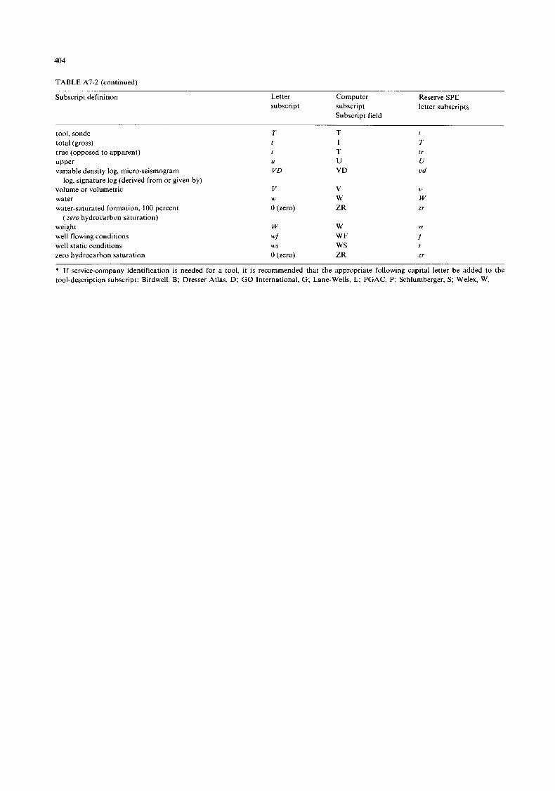
404
TABLE Al-2 (continued)
Subscript definition Letter Computer Reserve SPE subscript subscript letter subscripts
Subscript field
tool, sonde total (gross) true (opposed to apparent) upper variable density log, micro-seismogram
volume or volumetric water
log. signature log (derived from or given by)
T T r T r T U U VD VD
V V W W
f
T f r U vd
1)
W water-saturated formation, 100 percent 0 (zero) ZR zr
(zero hydrocarbon saturation) weight W W W
well flowing conditions wf W F f well static conditions ws ws S
zero hydrocarbon saturation 0 (zero) ZR zr
* If service-company identification is needed for a tool, it is recommended that the appropriate following capital letter be added to the tool-description subscript: Birdwell, B; Dresser Atlas, D; GO International, G; Lane-Wells, L; PGAC. P; Schlumberger, S; Welex, W.
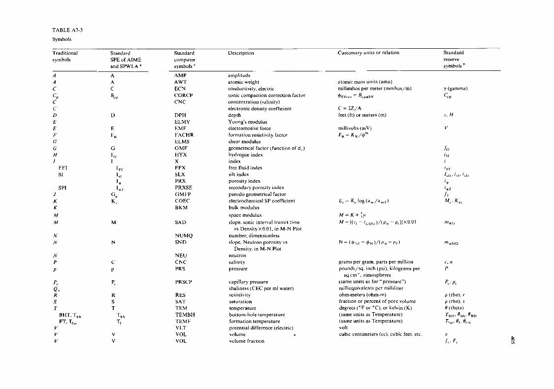
TABLE Al-3
Symbols
Traditional Standard Standard Description Customary units or relation Standard symbols SPE of AIME computer reserve
and SPWLA a symbols a symbols
A A C
C C D E E F G G H I
C P
FFI s1
SPI J K K
M M
N N
N P P
pc Q" R S T
BHT, T b h
m, T f m V V V
A A C BCP
D
E FR
G
I I H
I Ff
I, , 1, I,,
GP K c
M
N
C P
pc
R S T
Tbh
Tf
V V
AMP AWT ECN CORCP C N C
DPH ELMY EMF FACHR ELMS G M F HYX X FFX SLX PRX PRXSE G M F P COEC BKM
SAD
NUMQ SN D
N EU CNC PRS
PRSCP
RES SAT TEM TEMBH TEMF VLT VOL VOL
amplitude atomic weight conductivity, electric sonic compaction correction factor concentration (salinity) electronic density coefficient depth Young's modulus electromotive force formation resistivity factor shear modulus geometrical factor (function of d , ) hydrogen index index free fluid index silt index porosity index secondary porosity index pseudo geometrical factor electrochemical SP coefficient bulk modulus space modulus slope. sonic interval transit time
number. dimensionless slope. Neutron porosity vs
Density. in M-N Plot neutron salinity pressure
vs Density XO.01. in M-N Plot
capillary pressure shaliness (CEC per ml water) resistivity saturation temperature bottom-hole temperature formation temperature potential difference (electric) volume volume fraction
atomic mass units (amu) millimhos per meter (mmhos/m) +svcor = Bcp,sv
C = 2Z/A feet (ft) or meters (m)
millivolts (mV) F R = K,/+"
grams per gram, parts per million pounds/sq. inch (psi), kilograms per
(same units as for "pressure") milliequivalents per milliliter ohm-meters (ohm-m) fraction or percent of pore volume degrees (OF or "C). or kelvin ( K ) (same units as Temperature) (same units as Temperature) volt cubic centimeters (cc). cubic feet. etc.
sq cm ', atmospheres
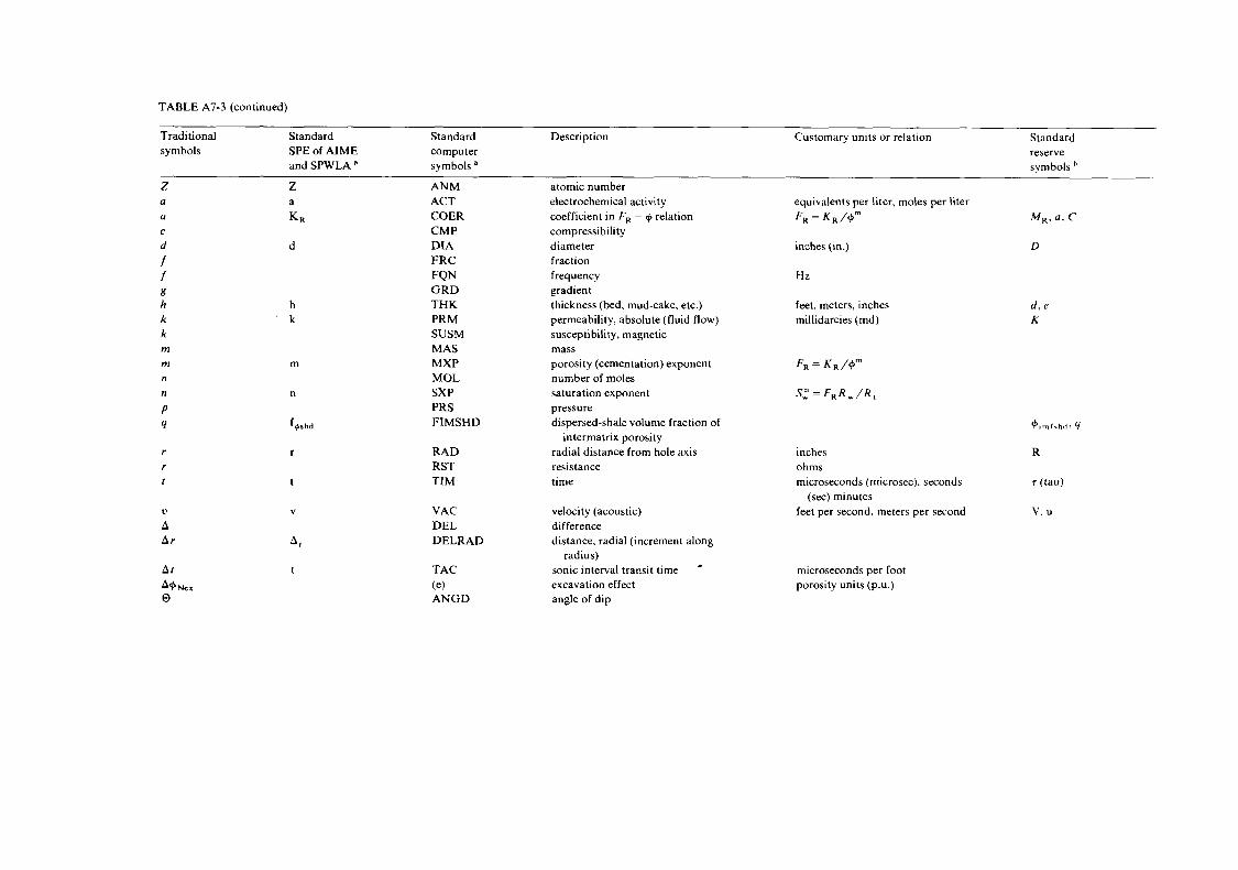
TABLE A7-3 (continued)
Traditional Standard Standard Description Customary units or relation Standard symbols SPE of AIME computer reserve
Z Z ANM atomic number
symbols and SPWLA a symbols a
Q a ACT electrochemical activity equivalents per liter, moles per liter Q KR COER coefficient in FR - + relation FR = KR/+" M R , C C CMP compressibility d d DIA diameter inches (in.) D f FRC fraction f FQN frequency Hz g G R D gradient h THK thickness (bed, mud-cake, etc.) feet, meters, inches k PRM permeability, absolute (fluid flow) millidarcies (md) k SUSM susceptibility, magnetic m MAS mass
n MOL number of moles
P PRS pressure 4 FIMSHD dispersed-shale volume fraction of
r RAD radial distance from hole axis inches r RST resistance ohms t TIM time microseconds (microsec), seconds
m MXP porosity (cementation) exponent F R = K R / + "
n SXP saturation exponent S: = F , R , / R ,
intermatrix porosity
(sec) minutes
h k
d , e K
m
n
+ps hd
r
t
0
A A r
V
A ,
t
VAC velocity (acoustic) DEL difference DELRAD distance, radial (increment along
radius) TAC sonic interval transit time * (e) excavation effect ANGD angle of dip
feet per second, meters per second
microseconds per foot porosity units (P.u.)
+ l r n l \ h d . 4
R
r (tau)
v. u
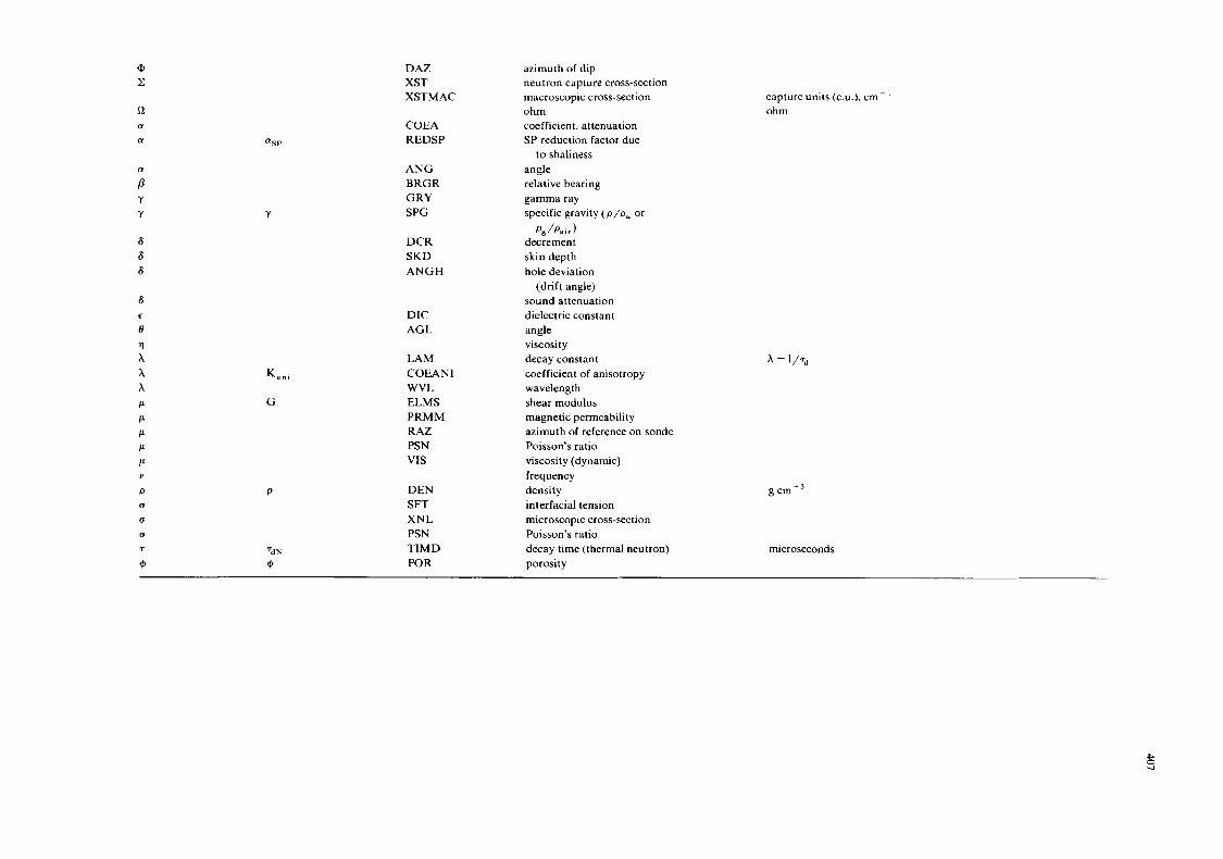
a a
a
a
P Y Y
6 s s
8
0 1)
h h h P P P P P
P a
a
€
Y
U
7
+
Y
Kani
G
P
‘d N
@
DAZ XST XSTMAC
COEA REDSP
ANG BRGR CRY SPG
DCR SKD ANGH
DIC AGL
LAM COEANI WVL ELMS PRMM RAZ PSN VIS
DEN SFT XNL PSN TIMD POR
azimuth of dip neutron capture cross-section macroscopic cross-section ohm coefficient, attenuation SP reduction factor due
to shaliness angle relative bearing gamma ray specific gravity ( p / p , or
decrement skin depth hole deviation
(drift angle) sound attenuation dielectric constant angle viscosity decay constant coefficient of anisotropy wavelength shear modulus magnetic permeability azimuth of reference on sonde Poisson’s ratio viscosity (dynamic) frequency density interfacial tension microscopic cross-section Poisson’s ratio decay time (thermal neutron) porosity
PJP, I r )
capture units (c.u.), cm- ’ ohm
h = 1/Td
g cm-3
microseconds
P 0 4
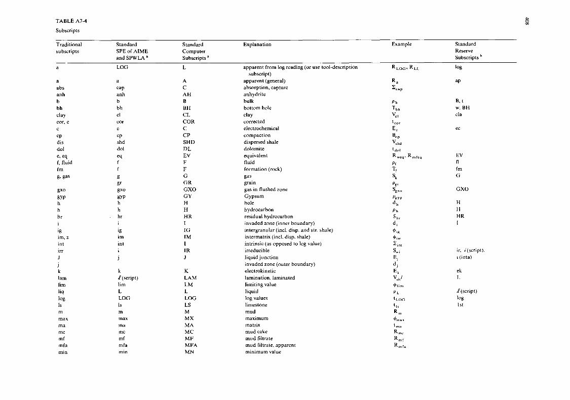
TABLE A7-4
Subscripts
P 0 W
Traditional subscripts
Standard SPE of AIME and SPWLA a
a
a abs anh b bh clay cor, c
CP dis do1 e, eq f, fluid fm g. gas
C
gxo gyp h h hr I
ig im, z int irr J
k lam lim liq log Is m max ma mc mf mfa min
j
LOG
a cap anh b bh cl cor
CP shd do1 eq f f g gr &uo gyp h h hr
ig im int
C
I
1
j
k P(script) lim L LOG Is m max ma mc mf mfa min
Standard Computer Subscripts a
L
A C AH B BH CL COR C CP SHD DL EV F F G GR GXO GY H H HR I IG IM I IR J
K LAM LM L LOG LS M MX MA MC M F MFA MN
Explanation Example Standard Reserve Subscripts
apparent from log reading (or use tool-description
apparent (general) absorption, capture anhydrite bulk bottom hole clay corrected electrochemical compaction dispersed shale dolomite equivalent fluid formation (rock) gas grain gas in flushed zone Gypsum hole hydrocarbon residual hydrocarbon invaded zone (inner boundary) intergranular (incl. disp. and str. shale) intermatrix (incl. disp. shale) intrinsic (as opposed to log value) irreducible liquid junction invaded zone (outer boundary) electrokinetic lamination, laminated limiting value liquid log values limestone mud maximum matrix mud cake mud filtrate mud filtrate, apparent minimum value
subscript)
B. t w, BH cla
ec
EV n fm G
GXO
H H HR I
ir. i(script). L (iota)
ek L
P (script) 1% 1 St
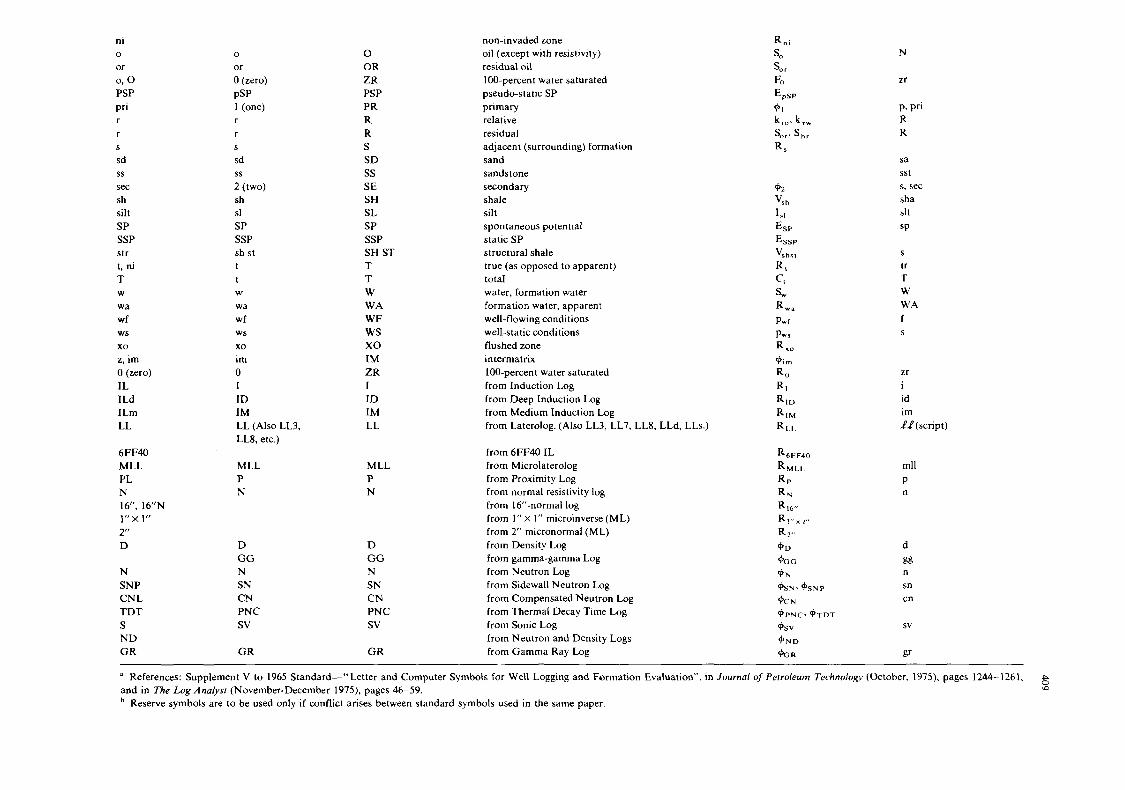
ni
or 0, 0 PSP pri r r
sd
sec sh silt SP SSP str t, ni T
wa wf
0
S
ss
W
ws xo z, im 0 (zero) IL 1Ld ILm LL
6FF40 MLL PL N 16", 16'" 1" x I" 2" D
N SNP CNL TDT S ND GR
0
or 0 (zero) PSP 1 (one) r r
sd S
ss 2 (two) sh sl SP SSP sh st t t W
wa wf ws xo im 0 I ID IM LL (Also LL3, LL8, etc.)
MLL P N
D GG N SN CN PNC sv
GR
0 OR ZR PSP PR R R S SD ss SE SH SL SP SSP SH ST T T W WA WF ws xo IM ZR I ID IM LL
MLL P N
D GG N SN CN PNC sv
G R
non-invaded zone oil (except with resistivity) residual oil 100-percent water saturated pseudo-static SP primary relative residual adjacent (surrounding) formation sand sandstone secondary shale silt spontaneous potential static SP structural shale true (as opposed to apparent) total water, formation water formation water, apparent well-flowing conditions well-static conditions flushed zone intermatrix 100-percent water saturated from Induction Log from Deep Induction Log from Medium Induction Log from Laterolog. (Also LL3, LL7, LL8, LLd, LLs.)
from 6FF40 IL from Microlaterolog from Proximity Log from normal resistivity log from 16"-normal log from I" x 1 " microinverse (ML) from 2" micronormal (ML) from Density Log from gamma-gamma Log from Neutron Log from Sidewall Neutron Log from Compensated Neutron Log from Thermal Decay Time Log from Sonic Log from Neutron and Density Logs from Gamma Ray Log
N
zr
p, pri R R
sa
s, sec sha slt SP
SSt
S
tr T W WA f S
zr i id im .!..!(script)
mll P n
a References: Supplement V to 1965 Standard-"Letter and Computer Symbols for Well Logging and Formation Evaluation". in Journal of Perroleurn Technology (October, 1975). pages 1244-1261. P
and in The Log Analysr (November-December 1975). pages 46-59. s Reserve symbols are to he used only if conflict arises between standard symbols used in the same paper.
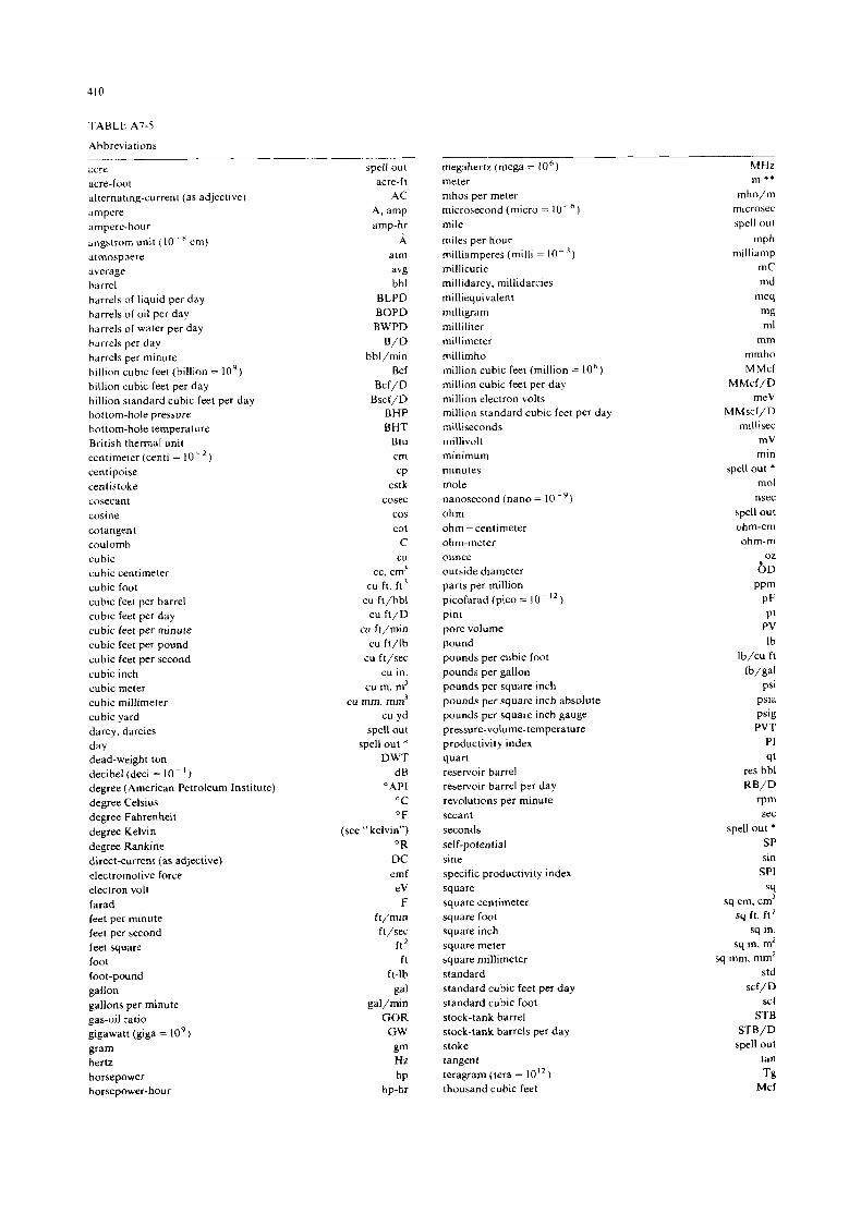
410
TABLE Al-5
Abbreviations
acre acre-foot alternating-current (as adjective) ampere ampere-hour angstrom unit cm) atmosphere average barrel barrels o f liquid per day barrels of oil per day barrels of water per day barrels per day barrels per minute billion cubic feet (billion = 10') billion cubic feet per day billion standard cubic feet per day bottom-hole pressure bottom-hole temperature British thermal unit centimeter (centi = lo-') cent ipoise centistoke cosecan t cosine cotangent coulomb cubic cubic centimeter cubic foot cubic feet per barrel cubic feet per day cubic feet per minute cubic feet per pound cubic feet per second cubic inch cubic meter cubic millimeter cubic yard darcy. darcies
dead-weight ton decibel (deci = 10- ' )
degree (American Petroleum Institute) degree Celsius degree Fahrenheit degree Kelvin degree Rankine direct-current (as adjective) electromotive force electron volt farad feet per minute feet per second feet square foot foot-pound gallon gallons per minute gas-oil ratio gigawatt (giga = lo9) gram hertz horsepower horsepower-hour
day
spell out acre-ft
AC
amp-hr
atm avg bbl
BLPD BOPD BWPD
bbl/min Bcf
Bcf/D Bscf/D
BHP BHT
Btu cm CP
cstk cosec
A, amp
A
B/D
cos cot
C cu
cc, cm' cu ft, ft '
cu ft/bbl cu f t /D
cu ft/min cu ft/lb
cu ft/sec cu in.
cu m. m' cu mm. mm'
cu yd spell out
spell out * DWT
dB "API
"C O F
(see "kelvin") "R
DC emf eV
F ft/min ft/sec
f t 2 ft
ft-lb gal
gal/min GOR
GW gm Hz hP
hp-hr
megahertz (mega = 10') meter mhos per meter microsecond (micro = lo-') mile miles per hour milliamperes (miIIi = 10- ') millicurie millidarcy, millidarcies milliequivalent milligram milliliter millimeter millimho million cubic feet (million = 10') million cubic feet per day million electron volts million standard cubic feet per day milliseconds millivolt minimum minutes mole nanosecond (nano =
ohm ohm - centimeter ohm-meter ounce outside diameter parts per million picofarad (pic0 =
pint pore volume pound pounds per cubic foot pounds per gallon pounds per square inch pounds per square inch absolute pounds per square inch gauge pressure-volume-temperature productivity index quart reservoir barrel reservoir barrel per day revolutions per minute secant seconds self-potential sine specific productivity index square square centimeter square foot square inch square meter square millimeter standard standard cubic feet per day standard cubic foot stock-tank barrel stock-tank barrels per day stoke tangent teragram (tera = 10") thousand cubic feet
MHz m **
mho/m microsec spell out
milliamp mC md
meq mg ml
mm mmho MMcf
MMcf/D meV
MMscf/D millisec
mV min
spell out * mol nsec
spell out ohm-cm ohm-m
mPh
02
b D PPm
PF Pt
PV Ib
Ib/cu f t Ib/gal
psi psia Psig PVT
PI 91
res bbl RB/D
rpm sec
spell out * SP sin
SPI
sq sq cm. cm2
sq ft, ft sq in.
sq m, m2 sq mm, mmz
std scf/D
sc f STB
STB/D spell out
tan TK
Mcf

41 1
hour hyperbolic sine. cosine. etc. inch inches per second inside diameter kelvin kilogram (ki lo = 10') kilohertz kilovolt kilowatt kilowatt-hour liquefied petroleum gas liter logarithm logarithm (natural) maximum
spell out * sinh. cosh. etc.
in. in . / sec
ID K
kHz kV
kW kW-hr
LPG spell out
1% In
max
kg
thousand cubic feet per day thousand standard cubic feet per day trillion cubic feet (trillion = 10") trillion cubic feet per day versus volt volume per volume water-oil ratio watt yard
Mcf/D Mscf/D
Tc f Tcf/D
V
WOR W
V b
vol/vol
Yd
* * *
Except in combinations such as ft/D, cc/sec. ft/hr Except with the number 1 : 1 meter. not I m.

This Page Intentionally Left Blank
413
INDEX AND GLOSSARY
Here below are listed the most common terms or expressions used in well logging, followed by a short definition or explanation.
When they are treated more fully in this book, only the relevant chapter is referred to.
Absorption: 1. the process of taking up by capillary, osmotic, chemical or
solvent action 2. the process by which energy such as that of electromagnetic
or acoustic waves, is converted into other forms of energy. - neutron absorption: 8.2.1.4. - gamma-ray absorption: 12.1 Accelerator:
a device which permits the acceleration of electrons or nuclear particles. For example, an accelerator is used to produce neu- trons by accellerating deuterium before striking a tritium target, in pulsed neutron logging. 10.3
of or pertaining to sound. acoustic impedance: the product of acoustic velocity and den- sity, 13.6.
Acoustic:
-
- acoustic log: 14. - acoustic signal: 13.1. - acoustic travel time: time required for an acoustic wave to
travel from one point to another. acoustic wave: a sound wave in which the disturbance propa- gated through a medium is an elastic deformation of the medium. 13.2
the process of making a substance radioactive by bombarding it with nuclear particles. For example irradiation by neutrons which transform some nuclei into radio-isotopes, which are characterized by the energy of the induced gamma ray and by their decay time schemes. 9.2.2.
Activity: 1. for a solution the thermodynamic equivalent concentration
ie. the ion concentration corrected for the deviation from ideal behaviour due to the interionic attraction of ions. 4.3.
2. the intensity of radioactive emission of a substance, mea- sured as the number of atoms decaying per unit of time. 6.2.6.
Adsorption:
-
Activation:
Adherence of gas molecules or of ions of molecules in solutions to the surfaces of solids with which they are in contact.
A-electrode: the current-emitting electrode in a resistivity-measuring device. 3.2.1.
the ratio of the pseudo-static SP (PSP) to the static SP (SSP). 4.6.1.2.1.
Alpha particle: 6.2.1.
AM: notation used to refer to the distance between the current electrode (A) and the potential measuring electrode (M). 3.2.1.1.
a curve recorded on a more sensitive scale.
Alpha:
Amplified curve:
Amplitude: the maximum value of the displacement in an oscillatory motion. 14. and 15.
system in which the information is represented as a continuous flow of the quantity constituting the signal.
1.3.3.2
I . that space between a drill pipe and the formation through which the drilling fluid returns to the surface.
2. the space between casing and formation or between tubing and casing.
3. a ring of interstitial water sometimes produced by invasion processes in hydrocarbon-bearing beds. When R /(, > R,,, the annulus will be more conductive than the flushed zone ( R x o ) or the virgin zone (R,).
Analog system:
Anisotropy:
Annulus:
AO: notation used to refer to the distance between the current electrode (A) and the point (0) midway between the potential measuring electrodes. 3.2.1.2.
abbreviation for American Petroleum Institute.
is the standard format used by all logging companies for recording well logging measurement. This grid has:
- one left-hand track, 2.5 inches wide, - the depth track or column, 0.75 inch wide,
~ two right-hand tracks, 2.5 inches wide each. The tracks may be divided into a linear or logarithmic scale. 2.4.
calibration pits at the University of Houston for gamma ray: 6.1 I .
API:
API log grid:
API test pits:
-
- for neutron: 8.2.5. API unit:
( I ) for gamma-ray curves: the difference in curve deflection between zones of low and high radiation in the API gamma-ray calibration pit is 200 API gamma-ray units. 6.2.6. and 6. I I .
(2) for neutron curves: the difference between electrical zero and the curve deflection opposite a zone of Indiana limes- tone (19% porosity) in the API neutron calibration pit is 1,000 API units. 8.2.5.
Apparent:
Archie: as recorded, before correction for environmental influence.
engineer of the Shell Company who found the relationship between the formation resistivity factor, the porosity and the water saturation. 1.4.2
a bow spring or lever connected to a logging sonde which presses against the borehole wall to centralize the tool, to push the tool to the opposite side of the borehole, or to hold a sensor pad to the borehole wall.
a display of dipmeter data. 19.6.2.1.
symbol AMU: a measure of atomic mass, defined as equal to 1/12 mass of a carbon of mass 12.
Arm:
Arrow plot:
Atomic mass unit:
414
Atomic number: symbol Z : number of protons within an atomic nucleus, or the number of orbital electrons in a neutral atom
symbol A : the relative weight of an atom on the basis that carbon is 12. Equal to the total number of neutrons and protons in the atomic nucleus.
Attenuation: 15.
Azimuth: I . In the horizontal plane, i t is the clockwise angle of departure
from magnetic north. 2 Curve recorded in dipmeter survey. I t is the clockwise angle
from magnetic north to the reference electrode (no.1) on the sonde. 19.5.
Azimuth frequency plot:
Atomic weight:
a diagram on polar chart paper which presents only a count of how many dip azimuth measurements fall within each ten degree sector, within a given group of dips. Dip magnitude is ignored. 19.6.2.3.
Back-up: a curve recorded by a back-up galvanometer, which begins to record when the primary galvanometer has reached the limit of available track width or goes off scale.
10- 2 4 cm2/nucIeus: a unit for measuring capture cross-sections of elements.
Base-line shift: I . generally refers to a naturally occurring shift of the base line
of any specific curve (SP or GR ... ). Usually the base line referred to is the shale base line.
2. sometimes refers to a manual shift made by the logging engineer.
Barn:
Beta particle: a high-speed disintegration electron spontaneously emitted
from an atomic nucleus as a form of radiation. 6.2.2. BHC:
Borehole Compensated Sonic log. 14.2 BHT:
Bottom hole temperature. Bimetallism:
4.5.8.1. Blind zone:
shadow zone. Commonly observed on curves recorded by a lateral device. 3.2.6.2.2.
a convention used in dipmeter interpretation. I t corresponds to an increasing dip magnitude with decreasing depth with nearly uniform azimuth.
the ratio of attenuation in zone of interest (db/ft) to attenua- tion in well-cemented section (db/ft). I t is an indicator of the quality of cement bond. 15.3.
the spurious influence on a well-logging measurement due to the influence of the borehole environment which includes: hole diameter, shape of the borehole wall (rugosity), type of bore- hole fluid, mud-cake.
21.1.
1. water which has become adsorbed to the surfaces of solid particles or grains. Under natural conditions this water tends to be viscous and immobile but might not have lost its electrolytic properties.
2. water which is chemically bound by becoming part of a crystal lattice. This water has lost its electrolytic properties.
Blue pattern:
Bond index:
Borehole effect:
Borehole televiewer:
Bound water:
Bridle: 2.3.2.4.
Bulk density: symbol pb: i t is the value of the density of rock as its occurs in nature. 11.3
Bulk modulus: symbol K : 13.3
Button: a small disc-shaped, button-like electrode used on micro-resis- tivity pads (ML, MLL, H D T . . . ).
Cable: 2.3.2.
Calibration: the process wherein the scale and sensitivity of the measuring circuit is adjusted to meaningful units. 2.5.
17.
1. recorder. An instrument which records traces of light which have been beamed on film by galvanometers responsive to logging tool measurements. 2.3.4.1.
2. borehole camera: downhole instrument which photographs the interior of the borehole or casing.
Caliper:
Camera:
Capture cross-section: 1. the nuclear capture cross section for neutrons is the effective
area within which a neutron has to pass in order to be captured by an atomic nucleus. It is often measured in barns.
2. macroscopic capture cross section, symbol 2, is the effective cross-sectional area per unit volume of material for capture of neutrons. 10.2.1.2. e
Capture unit: symbol C.U. =
capture cross section: equivalent to sigma unit. 10.6. Carbon/oxygen:
9.2.6. C/O is a Dresser Atlas trademark. Cartridge:
a package which contains electronic modules or hardware for the down hole instrument. The package is carried in a protec- tive housing. 2.3.3.
Casing collar locator: symbol CCL: a coil and magnet system used to locate casing collars.
symbol CEC: a measure of the extent to which a substance will supply exchange cations. Compensating cations serve to com- pensate the excess of charge (usually negative) in clay lattice. I t is related to the concentration of compensating cations near clay-layer surfaces, which in the presence of water can be exchanged for other cations available in solution. The CEC is expressed in terms of milliequivalents of exchangeable ions per 100 grams of dry clay. 1.3.3.3.
a membrane which permits the passage of cations but not of anions. Clay acts as a membrane. 4.2.1.
Cement Bond Log. 15.3.1.
symbol m : the porosity exponent in Archie's formula. 1.4.1.
symbol CBL: used to determine the presence of cement behind casing and the quality of cement bond to casing or formation wall. 15.3.1.
a device which positions the logging tool in the center or near the center, of the well bore, aligned with the well bore axis.
cm- I . A unit of measure of macroscopic
Cation exchange capacity:
Cationic membrane:
CBL:
Cementation factor:
Cement bond log:
Centralizer:
415
Channel: I . a defect in cement quality which prevents zone isolation 2. in a pulse height analyzer. an energy gate in which only
pulses occurring within a specific energy range are reg- istered. The width of the channel corresponds to the dif- ference between the upper and lower limits.
3. a path along which digital or other information may flow in a computer.
Chlorine log:
Clean:
Combination logging tool:
9.1.1. and 9.1.3.
containing no appreciable amount of clay or shale.
a single assembly of logging tools capable of performing more than one general type of logging service with a single trip into the well bore, so saving rig time. 2.3.5.
symbol Cp or cAt, ,: an empirical correction applied to porosity derived from the sonic log in uncompacted formations. 14.8.
the Quick-Look Interpretation of well logs often requires a direct comparison of log responses (i.e. p b vs. + N ) . In order to facilitate this comparison, the same grid type and equal scale sensitivities must be used. Overlay techniques require the use of compatible scales
corrected out unwanted effects associated with the borehole. Compensated formation density log: symbol FDC: 11.7. FDC is a Schlumberger registered trademark
- Compensated neutron log: symbol CNL: 8.2.6. CNL is a Schlumberger registered trademark. Compensated sonic log: symbol BHC: 14.2
several well logs on the same interval of a well, spliced together to form a single continuous record for correlation purposes.
symbol C: the volumetric change in a unit volume of fluid when the pressure on that volume is increased. 13.3
Compressional wave: symbol P-Wave: 13.2.1.
Compton scattering: 11.1.2.
Conductivity: the property of a solid or fluid medium which allows the medium to conduct a form of energy (electricity, temperature ...). 1.3.3.2.
pertains to a rock framework provided with a degree of cohesiveness or rigidity by cementation or other binding means.
a genetic term referring to the log produced by any logging tool which uses pad or skid devices to make direct contact with the formation wall.
Continuous velocity log: symbol CVL: see SoNc Log 14.
Correlation interval: 19.5.4.2.
Crossplot: a plot of one parameter versus another.
Crosstalk: 4.5.8.2.
Curie: a standard measure of the rate of radioactive decay. 6.2.6.
Cycle skip: 14.9.2.
Compaction correction:
Compatible scale:
Compensated :
-
~
Composite log:
Compressibility:
Consolidated:
Contact log:
Darcy: a unit of permeability: 1.4.5.
Dead-time: i t corresponds to the recovery period, required by the system to prepare itself for counting each successive event. Events occur- ring during dead-time are not counted. 5.4.
the spontaneous disappearance of an effect radioactive decay: 6.2.4 thermal decay time: 10.
the measurement of formation properties far enough from the well bore that the effects of the invaded zone become minimal.
1. the internal movement in a galvanometer, in response to an impressed voltage, which produces the excursion on a log- ging trace or curve.
2. the lateral movement or excursion of a curve. Delaware:
an anomalous effect on early Laterolog first observed in the Delaware Basin. 3.3.2.5.4.
a memorizer panel.
symbol p : mass per unit volume
11.
graphs which show the influence of various conditions on the basic measurement.
the depth track (see API log grid).
the zero depth reference for well logging. Usually kelly bushing, but could be ground level, derrick floor.. . .
to put in depth different well-logging measurements.
the radial depth from the wellbore to which mud filtrate has invaded porous and permeable rock. 2.2.1.2.
radius of investigation.
a sensor used for the detection of some form of energy.
1. departure of a borehole from vertical 2. angle measured between tool axis and vertical
derrick floor
symbol d , : the diameter to which mud filtrate has invaded porous and permeable rock. 2.2.1.2.
a material having low electrical conductivity compared to that of a metal.
relative permittivity. 16.1.
1. of ions. The spontaneous flow of ions from a more con- centrated solution into a more dilute solution. 4.2.2. 2. of thermal neutrons. 8.2.1.3. and 10.2.2.
liquid-junction potential. 4.2.2.
representation of quantities in discrete (quantized) units. The information is represented as a series of discrete numbers.
convert data from analog trace records to binary computer useable numbers.
Decay:
Deep investigation:
Deflection:
Delay panel:
Density:
Density log:
Departure curves:
Depth column:
Depth datum:
Depth matching:
Depth of invasion:
Depth of investigation:
Detector:
Deviation:
D F :
Diameter of invasion:
Dielectric:
Dielectric constant:
Diffusion:
Diffusion potential:
Digital:
Digitize:

416
Diode error: an unwanted portion of the total electrical conductivity signal sent to the surface from downhole induction logging instru- ments. The diode error is produced by the measure circuit electronics of the induction cartridge. It is isolated and mea- sured during the calibration operation at a step where the sonde output is zero. Once evaluated. it is cancelled during the survey operation.
Dip: the angle that a surface makes with the horizontal. 19.
Dipmeter: 19.
Directional survey: measurement of drift, azimuth and inclination of a borehole with vertical.
said of a formation which contains appreciable amount of clay or shale.
a term used to refer to particles (clays) distributed within the interstices of the rock framework. I .4.4.2.
the attitude of a borehole, the drift angle or deviation is the angle between the borehole axis and the vertical.
Dual induction: combination of a deep reading with a medium investigating. 3.3.1.8.5.
Dual Laterolog: combination of a deep and shallow laterologs. 3.3.2.1.4. Dual Laterolog is a Schlumberger registered trademark.
tool with two detectors with different spacings from the source. This configuration allows to decrease the borehole influence.
Dirty:
Dispersed:
Drift:
Dual spacing:
Eccentering arm: eccentralizer. A device which presses the sonde body against the borehole wall.
symbol k,: The ability of a rock to leave a fluid flow through it in the presence of fluid immiscible with the first. 1.4.5.1.3.
1. interconnected pore volume occupied by free fluids. Hydro-
2. also electrically effective porosity.
oxidation-reduction potential.
13.3
the name given in 1932 by C. and M. Schlumberger and E.G. Leonardon to a series of well surveying operations in open hole.
a genetic term used to refer to the combination SP, short and long normals, lateral.
the recorded output of the electronic measure circuit when no signal is being measured,
corresponds to an interval of depth in which log response is near constant. 2.2.2.3.
Electrochemical potential: 4.2. I .
Electrofacies: the set of log responses that characterizes a sediment and permits the sediment to be distinguished from other.
4.1.
Effective permeability:
Effective porosity: symbol +e:
dynamically effective pore volume. 1.3.3.1.
Eh:
Elastic cons tan t s :
Electrical coring:
Electrical survey:
Electrical zero:
Electrobed:
Electrofiltration potential:
Electrokinetic potential: 4.1.
Electrolyte: 1. material in which the flow of electric current is accompanied
2. any chemical compound which when dissolved in a solvent by a movement of ions.
will conduct electric current. Electronic density:
Electron volt: symbol p,: electron population per unit volume. 11.2.
symbol eV: a unit of energy equal to the kinetic energy acquired by a charged particle carrying unit electronic charge when it is accelerated a potential difference of one volt. Equiva- lent to 1.602 x 10- 19, joule.
a neutron which has been slowed down to a low energy level. in the range 100 eV-0.1 eV. 8.2.1.2.
a decrease in the neutron log apparent porosity reading below that expected on the basis of the hydrogen indices of the formation component. 8.2.10.
Epithermal neutron:
Excavation effect:
Fast neutron:
Fast-plot:
FFI:
a neutron of 100 KeV or greater energy.
19.6.2.5.
free fluid index: other symbol +f: the percent of the bulk volume occupied by fluids which are free to flow as measured by the nuclear magnetism log (NML). 21.3.
fracture identification log. 19.8.
symbol FR: refers to the depth of the first useable reading or value recorded on a curve.
a foreign object lost in the borehole.
formation interval tester: 20.2.2.
a term used to refer to a pad that does not make good contact with the borehole wall to record quality information.
the zone at a relatively short radial distance from the borehole, immediately behind mud cake, which is considered to be flushed by mud filtrate.
refers to a well log produced by any well logging device in which survey-signal sent by the tool is focused. 3.3. and 3.5.
a general term applied in well logging industry to the external environment of the drilled well bore without stratigraphic connotation.
symbol F factor derived from the porosity following law F = a / + ”
Formation interval tester: symbol FIT: 20.2.2.
Formation resistivity factor: symbol FR: 1.4.1.
Formation signal: the signal related to the formation.
Formation tester: symbol FT: 20.2.1.
Formation water: water present on the virgin formation.
FR: first reading.
FIL:
First reading:
Fish:
FIT:
Floating pad:
Flushed zone:
Focused log:
Formation:
Formation factor:
417
Free fluid index:
Free pipe:
Free point:
symbol FFI or @ f , see FFI.
pipe in a well bore which is free to vibrate
the deepest depth in the well bore that stuck casing or drill pipe is free and can be salvaged.
I . the number of cycles or waves in a unit of time: symbol f:
2. the number of occurrences or events over a specified period
Frequency:
13.
of time or length of borehole. Fresh:
FT: very low in dissolved salt.
formation tester: 20.2.1.
Galvanometer: a small voltmeter which has a miniature mirror fastened to the moving coil. Light from a source is directed onto the mirror from which it is reflected onto a moving photographic film where it traces a curve. 2.3.4.1.
equivalent to density log
electromagnetic radiation emitted from an atomic nucleus dur- ing radioactive decay. 6.2.3.
Geiger-Mueller counter, ionization chamber or scintillation counter are gamma-ray detectors.
an encapsulated radioactive material which emits gamma rays. Usually I3'Cs. 11.4.
a window or opening, usually in time, during which certain measurements are made. 6.5.
a type of gamma-ray detector. 6.5.
symbol G : 3.3.1.2.
ground level.
gas-oil ratio
the change in any parameter per unit change of another param- eter.
the density of a unit volume of a mineral or other rock matter at zero porosity.
a combination of logs or a computation procedure for calculat- ing the depth of invasion and the resistivity of both invaded and virgin zones.
a convention used in dipmeter interpretation. It represents a succession of dips of relatively constant azimuth and magni- tude.
Grid: see API log grid
Groningen effect: 3.3.2.5.5.
Guard electrode: electrode which carries electrical current which tends to confine the survey portion of the current flow to a thin horizontal layer.
Gamma-gamma:
Gamma ray:
Gamma-ray detector:
Gamma-ray source:
Gate:
Geiger-Mueller counter:
Geometrical factor:
GL:
GOR:
Gradient:
Grain density:
Grand slam:
Green pattern:
Half-life: the time required for any amount of radioactive nuclide to lose one-half of its original activity by decay. 6.2.4.
Half-thickness: the thickness of an absorbing material necessary to reduce the intensity of incident radiation by one-half 6.2.
the threaded connector end of downhole logging tool (sonde- cartridge set). 2.3.3.
the form attached to the top of a well log which displays all relevant information about the well, the survey, and the well- bore condition. 2.4.
symbol Hz: the measure of frequency. defined as equal to 1 cycle per second.
spurious high-resistivity anomalies found on induction-derived curves inside the upper or lower boundary of a resistive bed. A result of improper boundary compensation for the level of formation resistivity being logged.
any of the following criteria, found in a well bore, which will severely affect or restrict the logging operations:
- depth greater than 20,000 f t - temperature greater 325 "F - pressure greater than 20,000 psi - hole deviation greater than 50 - H, S or gas-cut mud. Housing:
a cylindrical metal case which protects the electronic cartridge of the downhole logging instrument from damage by pressure and moisture. 2.3.3.
a modified form of the Archie's relationship proposed by Humble Company. F = 0.62/@2.'5
a resistivity scale used with laterolog, below midscale, the scale is linear in resistivity; above midscale, the scale is still in resistivity units but is linear with conductivity.
an articulating, liquid-filled pad used to place current and measuring electrodes in direct contact with the borehole wall. I t allows better electrode contact by improving pad conformity with the wall.
symbol S,: fraction of the pore volume filled with hydro- carbon.
symbol I , : the ratio of the number of hydrogen atoms per unit volume of a material to that number in pure water at 75'F. 8.2.10.
the weight of formation fluid filling the pores of the rock and in communication with the water table at the well site, or sea surface.
Head:
Heading:
Hertz:
Horn:
Hostile environment:
Humble formula:
Hybrid scale:
Hydraulic pad:
Hydrocarbon saturation:
Hydrogen index:
Hydrostatic load:
IL: induction log. 3.3.1.
Impedance: 13.6.
Inclinometer: a device for measuring hole inclination and azimuth.
Induced: term related to any provocated phenomenon produced by excitation.
- induced polarisation - induced gamma ray - induced gamma-ray spectrometry. 9. Induction:
3.3.1.

418
Interval transit time:
Invaded zone: symbol A t or t : the travel time of a wave over a unit distance.
the portion of formation surrounding a well bore into which drilling fluid has penetrated, displacing some of the formation fluids. 2.2.1.2.
2.2. I .2.
atom or group of atoms which has either taken on or given up one or more orbital electrons.
a type of gamma-ray detector. 6.5.
i t corresponds to the minimum saturation of a fluid when the fluid is displaced from a porous medium by another fluid immiscible with the first.
atoms of a single element which have differing masses. It is either stable or unstable (radioisotope).
the property of homogeneity of a rock which allows it to show the same responses when measured along different axes.
Invasion:
Ion:
Ionization chamber:
Irreducible saturation :
Isotope:
Isotropy:
Junction: refers to liquid junction potential. 4.2.2.
KB: Kelly bushing: rotary drilling bushing. Often taken as a depth datum.
Lag: corresponds to the distance the detector moves, during one time constant
symbol LR: refers to the depth of the last useable reading or value recorded on a curve.
Lateral device: 3.2.1.2.
Laterolog: 3.3.2. Laterolog is a Schlumberger registered trademark.
Line: 1 . ground line 2. survey cable
4.2.2.
refers to the mineralogical composition and to the texture of a rock.
the weight of the overlying rock column without the fluid contained in the pore volume of the rock.
laterolog. 3.3.2.
I . a record containing one or more curves related to some property in the formation surrounding the well bore. 2.4.
2. to run a survey.
depth datum for the survey.
symbol P-Wave: see compressional wave. 13.2.1.
a resistivity curve recorded with a normal electrode configura- tion in which AM spacing is 64 inches.
last reading
Last reading:
Liquid-junction potential:
Lithology :
Lithostatique load:
LL:
Log:
Log zero:
Longitudinal wave:
Long normal curve:
LR:
Macroscopic anisotropy : 1.3.3.2.
Magnetism: 4.5.8.3.
Magnetostriction: the change in dimension of a body when subjected to a magnetic field.
converts electro-magnetic energy to mechanical energy and vice versa.
Manual shift: an intentional electrical or mechanical shift given to a curve by the engineer during a survey in order to keep the curve within a given track.
1. a magnetic mark or metal shin on a survey cable for
2. one of the marks on the left part of Track-1 of a log used to
Magnetostrictive transducer:
Mark:
depth-control.
compute logging speed. See Minute Mark. Matrix:
1. for log analyst the solid framework, except shale, of rock
2. for geologist the smaller or finer-grained, continuous material which surrounds pore volume. 1.3.1.
of a sediment or sedimentary rock. Maximum pressure rating:
corresponds to the maximum pressure for satisfactory opera- tion of the downhole instrument.
corresponds to the maximum temperature for satisfactory oper- ation of a downhole instrument.
millidarcy. 1.4.5.
corresponds to the depth measured along the drilled hole not corrected for hole deviation.
a depth reference point, on a logging sonde, at which measure- ments are taken.
the reading of a galvanometer at rest. With no potential ap- plied, this is the zero reference for galvanometer deflections.
the potential-measuring electrode nearest the A electrode in a resistivity-measuring device. 3.2.1.
an electronic storage device whch delays the measured signal to record at depth the different measuring points of a combined device. 2.3.6.
a unit of electrical conductance.
a unit of electrical conductivity. 3.4.1.
a very short lateral electrode arrangement.
symbol MLL: 3.5.1. MLL is a Schlumberger registered trade- mark.
Microlog: symbol ML: 3.4.1. ML is a Schlumberger registered trademark,
Micronormal: a very short normal electrode arrangement. 3.4.1.
Microresistivity log: a log of the resistivity of the flushed zone around a borehole (see ML, MLL, MSFL, PML).
1.3.3.2.
symbol MSFL: 3.5.3. MSFL is Schlumberger registered trademark.
Maximum temperature rating:
md:
Measured depth:
Measured point:
Mechanical zero:
M electrode:
Memorizer:
mho:
mho per meter:
Microinverse:
Microlaterolog :
Microscopic anisotropy :
Microspherically focused log:
419
Mineral: a naturally occurring material having a definite chemical com- position and, usually. a characteristic crystal form. entering in the composition of a rock (Table 1-1).
a neutron generator
a mark or grid line interruption which is placed on the film every 60 seconds during the survey, to control the logging speed. It is usually found near the outside edge of track I . 2.2.3.
mmho: millimho
MN spacing: the distance between the two potential measuring electrodes in a lateral device. 3.2.1.2.
of a fluid. 2.2.1.4.
a plot of dipmeter information on polar chart paper where 0" dip is represented on the circumference and 90' at the center, 19.6.2.4.
Monitor curve: a curve recorded on a well log which is a measure of some aspect of a tool performance or stability. An indicator to the quality of measurements being made by the instrument.
an armoured single conductor cable. 2.3.2.2.
a single electrode for measuring formation resistance.
movable oil plot
symbol MOP: a computed log, based on several logging opera- tions, prepared for the purpose of determining the presence and quality of movable hydrocarbon.
drilling mud.
the residue deposited on the borehole wall as the mud looses filtrate into porous. permeable formations. 2.2. I .2.
symbol p,: the density of the drilling mud. Measured in pounds per US gallon (Ib/gl) or in g/cm3.
the effluent of the continuous phase liquid of drilling mud which penetrates porous and permeable rock, leaving a mud cake on the drilled face of the rock. 2.2.1.2.
a log recorded with Microlog or microlateroiog sonde with the arms collapsed. so that the measuring pad loses contact with the formation wall and "reads" the mud resistivity at downhole conditions.
Mini iron:
Minute-mark:
Mobility :
Modified Schmidt diagram:
Monocable:
Mono electrode:
MOP:
Movable oil plot:
Mud:
Mud cake:
Mud density:
Mud filtrate:
Mud log:
Negative separation: a term used in reference to microlog curves to describe the condition where the longer spaced resistivity curve ( R 2 " ) reads a lower value than the shorter space curve ( R,..,l..). 3.4.3.
an electrically neutral, elementary nuclear particle having a mass of 1.0089 atomic mass unit (very close to that of a proton). 8.
Neutron generator: an electromechanical device operating at high voltage (125- 130 kV) which focuses a beam of high-energy deuterons on a target surface containing tritium. Nuclear fusion of the deuteron ions and target atoms produces high-energy (14 MeV) neutrons. 10.3.
Neutron:
Neutron lifetime log: symbol NLL: 10.2.4. NLL is Dresser Atlas registered trade- mark.
Neutron log: a log of a response related to the interaction of neutrons with matter. 8.
Neutron source: 1. an encapsulated radioactive material which produces neu-
2. a neutron generator. 10.3. Noise:
sudden spurious readings on a curve. Normal device:
3.2.1. I . Normalize:
to adjust two log curves in order that one value may be compared with the other.
Nuclear magnetic resonance: a phenomenon exhibited by atomic nuclei which is based on the existence of nuclear magnetic moments associated with quantized nuclear spins, 21.3.
symbol NML: a well log which is dependent on the alignment of the magnetic moment of protons (hydrogen nuclei) with an impressed magnetic field. 21.3.
trons. 8.2.4.
Nuclear magnetism log:
Ohm:
Ohm-meter:
Open hole:
Osmosis:
symbol Q: a unit of electrical resistance.
symbol Q-m: a unit of electrical resistivity.
uncased hole or portion of the hole.
the spontaneous flow of molecules of the solvent of a more dilute solution into a more concentrated solution when sep- arated from one another by a suitable semi-permeable mem- brane.
Overburden: geostatic load.
Oxidation-reduction potential: symbol Eh: redox potential
Overlay: to place one recorded curve over another to provide specific information with regard to lithology and fluid saturation.
Pad: see sidewall pad.
Pair production: 1 1 . 1 . 1 .
Permeability : symbol k: a measure of the ability of a rock to conduct a fluid through its connected pores. 1.4.5.
an expression representing the negative logarithm of the effec- tive hydrogen-ion concentration or hydrogen-ion activity.
11.1.3.
used with a scintillation crystal to make up a scintillation counter. The flash of light produced in a scintillating crystal strikes the sensitive surface of a photocathode in the photomul- tiplier causing the emission of a number of primary electrons. These electrons are drawn to an anode maintained at a higher potential whereupon a number of secondary electrons are emitted for each impinging electron. The secondary electrons are drawn to a second anode, maintained at a higher potential than the first, whereupon additional multiplication occurs. This process is repeated until the initial current has been multiplied about a million fold. 6.5.
pH:
Photoelectric absorption:
Photomultiplier:
420
Photon: a quantity of energy emitted in the form of electromagnetic radiation.
Poisson’s ratio: symbol a or Y: 13.3
Polar plot: plots on polar coordinate paper usually used to aid dipmeter interpretation. 19.6.2.4.
Porosity: symbol +: 1.3.3.1.
Porosity exponent: symbol m: the exponent of the porosity term in Archie’s formula. 1.4.1.
Porosity overlay: a log of porosity values computed from different logs plotted on top of each other.
a term usually used in reference to Microlog curves to describe the condition where the micronormal (2”) resistivity curve reads a higher value than the microinverse (1” x 1”) curve. This condition usually denotes the presence of mud-cake on the face of a porous, permeable formation. 3.4.3.
a device for making a continuous measurement of the angle and direction of borehole deviation during a survey. 18.3.
parts per million
a downhole logging instrument or a sonde.
similar to an ionization chamber. It is designed for the detec- tion of neutrons. A metal chamber is filled with gas, generally 3He which produces a (n, a) reaction or BF, which produces the (n,p) reaction. A central electrode is maintained at a positive voltage with respect to the shell (1300 V for ’He, 2500 V for BF,). When a neutron enters the chamber the gas produces ionizing particles.
the atomic nucleus of the element hydrogen. A positively charged hydrogen atom.
symbol PL: 3.5.2. PL is a Schlumberger registered trademark.
symbol J: a coefficient used for estimating uninvaded forma- tion resistivity from the response recorded by a laterolog de- rice.
symbol PSP: the static SP of a dirty rock.
porosity unit: one percent pore volume.
fast neutron (14 MeV) emitted by a neutron generator.
compressional wave. 13.2.1.
Positive separation:
Poteclinometer:
PPm:
Probe:
Proportional counter:
Proton:
Proximity log:
Pseudo-geometrical factor:
Pseudo-static SP:
p.u.:
Pulsed neutron:
P-wave:
Radiation: the emission and propagation of energy through space or matter. The speed of propagation is that of light. It requires no intervening medium for its transmission.
6.1.
a nuclide. A radioactive isotope which spontaneously emits particles (a or p ) or electromagnetic radiation (gamma rays) as it decays to a stable state.
surface acoustic wave in which the particle motion is elliptical and retrograde with respect to the direction of propagation.
Radioactivity:
Radioisotope:
Rayleigh wave:
Reading:
Receiver: a value taken from a curve at a specific depth.
a transducer used to receive a form of energy which has been propagated through the formation or induced in the formation.
a sonde In which the current and measure electrodes are interchanged according to a specific rule.
an electronic module designed to convert conductivity measure- ments into resistivity (in induction logging).
a device which records well-log data on film, chart or tape.
symbol Eh: a quantitative measure of the energy of oxidation. Oxidation is equivalent to a net loss of electrons by the substance being oxidized; reduction is equivalent to a net gain of electrons by the substance being reduced.
a convention used in dipmeter interpretation to denote decreas- ing formation dip with decreasing depth with a near constant azimuth.
Reflection peak: an increase in the value of resistivity recorded by a lateral device as the A electrode passes a thin highly resistive bed. 3.2.6.2.2.
Relative bearing: symbol p: in dipmeter interpretation, looking down the hole, i t is the clockwise angle from the upper side of the sonde to the
Reciprocal sonde:
Reciprocator:
Recorder:
Redox potential:
Red pattern:
reference electrode no. 1
symbol: k , . 1.4.5.1.3.
symbol RFT: 20.2.3.
Relative permeability:
Repeat Formation Tester:
Repeat section: a short section of a log, that is recorded in addition to the main survey section in order to provide an inter-run comparison of log similarity, and, therefore, instrument stability and repeata- bility.
Residual: that which remains after a removal or displacement process.
Residual oil: oil remaining in the reservoir rock after the flushing or invasion process, or at the end of a specific recovery process.
symbol R : specific resistance. 1.3.3.2.
symbol Z = R,/R,. The ratio of the resistivity of a formation bearing hydrocarbon to the resistivity it would have if 100% saturated with formation water. 1.4.2.
an interval of characteristic distortion on a normal curve across a resistive bed which has a thickness less than the AM spacing. 3.2.6.1.2.
repeat formation tester: 20.2.3.
the quality of roughness or irregularity of the borehole wall.
Resistivity:
Resistivity index:
Reversal:
RFT:
Rugosity:
Salinity:
Saturated: refers to the concentration of ions in solution.
1. containing as much as it can contain under given conditions
2. reached the limit of its measuring capacity.
symbol S : the percentage of the pore volume occupied by a specific fluid. 1.4.2.
of temperature and pressure.
Saturation:
42 I
Saturation exponent: symbol n: the exponent of the saturation term in Archie’s saturation equation. 1.4.2.
Sawtooth SP: 4.4.7.
SBR: shoulder bed resistivity 3.3.1.5.
Scale: 1. depth scale 2.4. 2. grid scale sensitivity. 2.4.
Scattered gamma-ray log: see density log. 1 1 .
Schmidt diagram: a polar plot where the azimuth indicates dip or drift direction and the distance from the origin indicates dip or drift magni- tude.
Scintillation: a flash of light produced in a phosphor by an ionization event.
Scintillation counter: a type of gamma ray detector. 6.5.
Screen: 1. a view screen on the camera or recorder. 2. a video Screen in a computerized logging truck.
in dipmeter interpretation, the angle which will define the depth interval along which a correlation will be searched. 19.5.4.3.
Search interval: the depth interval defined by the search angle.
Secondary porosity: porosity resulting from alteration of the formation caused by fractures, vugs, solution channels, dolomitization. 1.3.3.1
symbol SPI: an estimate of the secondary porosity, calculated from sonic log values in conjunction with either density or neutron log values, or porosity resulting from a cross-plot of density and neutron porosities.
a caliper. 17.
the magnitude of the deflection of a curve in response to a standard signal.
3.2.6.2.2.
a fine grained, thinly laminated or fissile, detrital sedimentary rock formed by compaction and consolidation of clay. silt or mud.
a line drawn through the deflections characteristic of shale on a SP curve, which is used as a reference in making measurements to determine the formation water resistivity and the shale percentage.
Shear modulus: 13.3.
Shear wave: symbol S-wave. 13.2.2.
Short normal curve: a resistivity curve recorded with a normal electrode configura- tion in which AM spacing is 16 inches.
effect of adjacent beds on a well-logging measurement.
a formation sample obtained with a wireline tool. 20.1.
an epithermal neutron log recorded with the neutron source and detector mounted in a skid which is pressed against the borehole wall and may cut into the mud-cake to minimize borehole effects on the measurement. 8.2.6.
Search angle:
Secondary porosity index:
Section gauge:
Sensi tivi ty :
Shadow zone:
Shale:
Shale base line:
Shoulder bed effect:
Sidewall core:
Sidewall neutron log:
Sidewall pad: a measuring device mounted on the end of an arm which projects from the sonde body during the survey.
symbol s.u.: capture unit. 10.6.
1. a meaningful response, to a well-logging instrument, which
2. any type of pulse sent into the formation.
a continuous record of the travel time for acoustic energy to pass from a transmitter to a single receiver separated by a specific distance called spacing. 14.1.
refers to the projecting portion of the body of a sonde, contain- ing emission and measuring devices, which is pressed firmly against the borehole wall.
Skin depth: 3.3.1.7.
Skin effect: 3.3.1.7.
Skip: see cycle skip. 14.9.2.
Slowing down: 8.2.1.2.
Soda plot: 19.6.2.2.
Sonar: a technique involving the measurement of the time interval between the emission of a focused acoustic signal and detection of the signal reflected from a distance surface.
a downhole instrument connected to a wireline. 2.3.3.
an unwanted portion of the total conductivity signal sent to the surface by the downhole induction logging instrument. It is generated by imperfections in the coils in the sonde. I t is isolated and measured during the calibration operation when the sonde is placed in a zero-signal medium (air). Once evaluated i t is cancelled during the survey operation.
symbol SL: an acoustic velocity log. 14.
refers to the source of radiation used in the nuclear logging (density, neutron, thermal decay time.. .).
spontaneous potential: 4.
the distance between certain electrodes or sensors, or between source and detector, or between transmitter and receiver.
the distance separating certain sensors, for instance two re- ceivers on the acoustic sonde.
the amount of radioactive isotope present per unit of element, generally expressed as curie per gram.
7.
symbol SFL: 3.3.3. SFL is a Schlumberger registered trade- mark.
noise: a spurious, unwanted event whch has been recorded on a curve.
used to describe the angular momentum of elementary particles or of nuclei: 21.3.
Spine-and-ribs plots: is used in the computation of the compensation to be added to
Sigma unit:
Signal:
can be detected or measured.
Single receiver A t curve:
Skid:
Sonde:
Sonde error:
Sonic log:
Source:
SP:
Spacing:
Span:
Specific activity:
Spectral gamma-ray log:
Spherically focused log:
Spike:
Spin:
422
the measured value of bulk density from the dual-spacing formation density logs. 11.7.
Spontaneous potential: symbol SP: 4.
SSP: static spontaneous potential. 4.4.
Stand-off: the distance separating a sonde from the wall of the borehole.
Static: at rest, immobile
Static spontaneous potential: symbol SSP. 4.4.
Statistical variations: 5.3.
Step: step distance in dipmeter computation process: 19.5.4.
Step profile: an idealized invasion profile which assumes an abrupt transi- tion from the flushed zone to the uninvaded zone. 2.2.1.2.
Stick plot: 19.6.2.6.
Stoneley waves: are boundary acoustic waves at a liquid-solid interface resulting from the interaction of the compressional wave in the liquid and the shear wave in the solid. By definition, the Stoneley wave must have a wavelength smaller than the borehole diame- ter.
Streaming potential: 4.1.
Strike: the direction or trend that a structural surface (bedding plane or fault plane) takes as it intersects a horizontal plane.
Structure: 1.4.
Surface conductance: electrical conductance occurring at the surfaces of some solid crystalline materials (such as clays) when they are exposed to aqueous solutions.
I . to take and record borehole geophysical measurements 2. the result of a well-logging operation, a well log.
shear wave. 13.2.2.
short forms or abbreviations used to identify well logging
Survey:
S-wave:
Symbols:
parameters. Appendix 7.
Tadpole plot:
TC:
TD:
Televiewer:
Telluric currents:
arrow plot. 19.6.2.1.
time constant. 6.3.
total depth.
see borehole televiewer 21.1.
earth currents originating as a result of variations in the earth’s magnetic field, or resulting from artifical electric or magnetic fields.
Temperature log: 18.
Test loop: a device used in the calibration of induction logging tools.
Test pill: an encapsulated radioactive material which serves as a portable source of gamma radiation for the calibration of some radioac- tivity logging tools.
Texture:
Thermal conductivity:
Thermal decay time:
1.4.
a measure of the ability of a material to conduct heat. I8
symbol 7 : the time for the thermal neutron population to fall to l /e (37%) of its original value. 10.2.1.1.
symbol TDT. 10.2.4.2. T D T is a Schlumberger registered trademark.
Thermal neutron: a neutron which has kinetic energy in the same order of magnitude as that due to the thermal motion of nuclei in the medium ( = 0.025 eV).
compact, having very low permeability.
symbol TC. 5.3.
downhole instrument (sonde and cartridge).
a quick-connecting and quick-disconnecting device, mounted near the head end of the survey cable, which provides strength and the means to manually connect electrical survey conduc- tors to the bridle and head.
the crookedness of the pore pattern. 1.4.1.
symbol TD: total depth reached by a specific logging tool.
symbol +t: the total pore volume in a rock. 1.3.3.1.
well log track on the APl grid.
any device or element which converts an input signal into an output signal of a different form.
a realistic profile in which the distribution of fluids in the invaded section beyond the flushed zone varies with increasing distance from the borehole.
see interval transit time.
a device which emits energy into the environment of the logging instrument
symbol S-wave: shear wave. 13.2.2.
acoustic travel time over a specific distance.
thickness of the stratigraphic unit measured along a line normal to the direction of extension of the unit.
symbol R , : the resistivity of the undisturbed, uninvaded rock.
symbol TVD: a log computed from well logs recorded in deviated holes, in which measured depths have been rectified to true vertical depth.
Thermal (neutron) decay time log:
Tight:
Time constant:
Tool:
Torpedo:
Tortuosity :
Total depth: .
Total porosity:
Track: *
Transducer:
Transition profile:
Transit time:
Transmitter:
Transverse-wave:
Travel time:
True bed thickness:
True resistivity:
True vertical depth log:
ULSEL:
Ultra Long Spaced Electric log: ultra long spaced electric log. A Chevron trademark.
symbol ULSEL: a well log recorded with the use of a modified long normal electrode configuration on a 5,000-foot bridle. The AM spacing can be made 75, 150. 600 or 1,000 feet. Difference between measured resistivities and anticipated resistivities calculated from conventional resistivity logs indicate nearby resistivity anomalies (previous nearby cased hole, salt domes).
423
Unconsolidated: pertains to a rock framework which lacks rigidity.
Variable density: variable intensity.
Variable density log: symbol VDL. 15.5.
Vector plot: arrow plot
Vertical resolution: the minimum thickness of formation that can be distinguished by a tool under operating conditions.
symbol p or Y: resistance of a fluid to flow.
Viscosity:
Water loss: a mud property: the measure of filtrate loss in a water base drilling mud under typical pressure conditions.
Water saturation: symbol S,: the percentage of the pore volume of a rock occupied by water.
symbol A . 13.1.3.
see wave train.
corresponds to a wavelet of several cycles resulting from the response of an elastic system to an acoustic energy impulse.
the acoustic wave train can be displayed in different modes: I. intensity modulated-time mode in whic!i the wave train is
2. amplitude-time mode in which the wave train is shown as a
Wavelength :
Wavelet:
Wave train:
Wave train display:
shown in the VDL form.
wiggle trace. 15.5.
Weak point: a machined connector or calibrated cable designed to break
under specific tensile stress. Well bore:
a borehole Well log:
a wireline log or borehole log. Wiggle trace:
a representation of the acoustic wave train in the amplitude-time mode.
Wireline log: a well log.
Young’s modulus: symbol E . 13.3.
Z/A: ratio of atomic number to atomic weight.
Z/A effect: 11.3
Z axis: a third dimension added to a cross-plot of two parameters in an X-Y plane. The Z axis is perpendicular to both X and Y axes.
REFERENCES
American Geological Institute, 1977. Glossary of Geology. Edited by R. Gary, R. McFee, Jr. and C. Wolf, Washington, D.C.
CRC Handbook of Chemistry and Physics, 1981-1982. 62nd Edi- tion, CRC Press, Inc., Boca Raton, Florida.
SPWLA, 1975. Glossary of terms and expressions used in &ell logging.
Sheriff, V.E., 1970. Glossary of terms used in well logging. Geo- physics, 35: 1 1 16- 1 139.

This Page Intentionally Left Blank