Journal of Petroleum Science and Engineering 186 (2020) 106696

Available online 16 November 20190920-4105/© 2019 The Authors. Published by Elsevier B.V. This is an open access article under the CC BY-NC-ND license(http://creativecommons.org/licenses/by-nc-nd/4.0/).

Interval inversion as innovative well log interpretation tool for evaluating organic-rich shale formations

N.P. Szab�o a,b,*, M. Dobr�oka a

a University of Miskolc, 3515, Miskolc-Egyetemv�aros, Hungary b MTA-ME Geoengineering Research Group, University of Miskolc, 3515, Miskolc-Egyetemv�aros, Hungary

A R T I C L E I N F O

Keywords: Interval inversion Genetic algorithm Wireline log Unconventional reservoir Total organic carbon Estimation accuracy

A B S T R A C T

The identification and detailed evaluation of unconventional hydrocarbon reservoirs require the application of advanced well logging data processing techniques. Since the number of the petrophysical properties such as porosity, water and hydrocarbon saturation, kerogen content, and fractional volumes of matrix components may exceed that of the observed wireline log types, currently used quick-look methods based on few well logs provide approximate solution to a part of the above petrophysical quantities. For instance, Passey’s method basically utilizes two well logs for identifying the sweet spots and estimating the total organic content (TOC). Local inversion techniques estimating the petrophysical parameters in a given depth are also limited because of low overdetermination (data-to-unknowns) ratio and hence are very sensitive to data noises. Instead of using traditional empirical methods and to avoid ambiguous solutions by local inversion evaluations, data of all wireline logs measured in a longer depth interval are simultaneously inverted to give more accurate estimate to the petrophysical parameters in a highly overdetermined inverse problem. The suggested interval inversion approach allows the determination of the fractional volumes of rock constituents with their estimation errors in a joint inversion procedure. As part of the inversion process, the forward problem is improved by using kerogen and pyrite effects corrected probe response functions. Synthetic modeling tests are made to detect the noise sensitivity and outlier resistance of the proposed inversion algorithm, while a float-encoded genetic algorithm variant of the interval inversion method is applied to invert real data measured in an organic-rich shale reservoir in Alaska, USA. The feasibility is demonstrated by a well agreement between the inversion derived TOC values and those of measured on core samples. The interval inversion method not only works reliably in the presented shale gas formations, but it can be extended to evaluating other types of unconventional reservoirs.

1. Introduction

The efficient interpretation of in situ information acquired by well logging tools is of primary interest in exploration of unconventional reservoirs. To extract the petrophysical properties from the observed data advanced well-log interpretation methods must be used, which provide accurate and reliable estimation for the assumed model pa-rameters. Among the great variety of low porosity and permeability hydrocarbon-bearing rocks, which are classified and detailed with their wireline log signatures by Ma and Holditch (2015), this study mostly concentrates on the evaluation of shale gas formations. In oilfield practice, empirical methods are usually applied for well log analysis, which aim the estimation of single parameters of the petrophysical model in separate interpretation procedures. The content of total

organic carbon (TOC) as one of the most important reservoir parameters is normally estimated by the overlay analysis of electrical resistivity and acoustic travel-time logs (Passey et al., 1990) or by the use of the probe response functions of the above wireline log types (Carpentier et al., 1991). Zhao et al. (2016) proposed another useful clay indictor calcu-lated from the compensated neutron and bulk density logs. The above empirical techniques require reliable preliminary information on the rock matrix, clay and fluid properties given in the probe response equations and on other geological parameters such as the level of maturity (LOM). These quantities do not vary quickly with depth; they are normally treated as specific (zone) constants in a bigger interval. On the other hand, the mineral composition of shale reservoirs must be also known before the analysis of well logs basically known from laboratory data. Having recognized the complexity of interpretation, several

* Corresponding author. Department of Geophysics, University of Miskolc, 3515, Miskolc-Egyetemv�aros, Hungary. E-mail address: norbert.szabo.phd@gmail.com (N.P. Szab�o).

Contents lists available at ScienceDirect

Journal of Petroleum Science and Engineering

journal homepage: http://www.elsevier.com/locate/petrol

https://doi.org/10.1016/j.petrol.2019.106696 Received 20 August 2019; Received in revised form 20 October 2019; Accepted 13 November 2019

Journal of Petroleum Science and Engineering 186 (2020) 106696

2

authors proposed a modification of the original Passey’s method (Son-dergeld et al., 2010; Wang et al., 2015; Renchun et al., 2015) or offered alternative (inversion-based) solutions for calculating the TOC and LOM (Bibor and Szab�o, 2016).

Instead of processing separated groups of wireline logs, the comprehensive (quantitative) interpretation of all available well logs seem to be more effective approach for identifying and characterizing unconventional formations. Exploratory statistical techniques such as principal component, cluster and factor analyses give detailed infor-mation on lithological similarities and the influential factors signifi-cantly affecting the detection and characterization of sweet spots (Puskarczyk et al., 2019), and allow improved estimation of shale vol-ume and permeability (Szab�o and Dobr�oka, 2018). Naeini et al. (2019) showed that deep learning approaches such as supervised artificial neural networks give a new perspective for petrophysical, pore-pressure and geomechanical characterization of unconventional reservoirs. However, with the above statistical techniques, the computation of estimation error of the resultant parameters is not feasible. Computer-aided well log interpretation has used geophysical inversion methods originally to calculate the petrophysical parameters with their estimation errors (Mayer and Sibbit, 1980). Well logging data are traditionally inverted separately in each depth along a borehole. Having barely more data than unknowns, a marginally overdetermined inverse problem is solved in a given depth. A relatively small ratio of data to unknowns sets a limit to the number of petrophysical parameters to be extracted, and makes the local inversion procedure rather sensitive to data noises, especially to outliers. In unconventional resource estima-tion, the use of local inversion methodology is unfavorable, since there are a great number of unknowns describing a multi-mineral rock (i.e., TOC, fluid contents and several matrix volumes). If the number of model parameters exceeds that of the data at a given depth, the inverse prob-lem becomes underdetermined resulting in ambiguous solution. In addition, a large number of zone parameters found in the probe response functions must be specified, which are not allowed to be estimated in a marginally overdetermined (local) inverse problem. The subjective de-cisions made on the zone constants may add further uncertainty to the estimation.

To improve the efficiency of inverse problem solution, we suggest the increase of overdetermination of the inverse problem. The interval inversion approach inverts all data of a greater depth interval in one interpretation procedure to estimate significantly smaller number of unknowns than data. In order to do that, the model parameters are expanded into series, and the number of expansion coefficients as the unknowns of the inverse problem are optimally chosen to set the required overdetermination ratio. Interval inversion of well logs reduces significantly the estimation errors of model parameters such as porosity, shale content, water saturation and matrix volume (Dobr�oka et al., 2016). By the automated estimation of zone parameters, it serves a more accurate forward problem solution and may reduce the high dependence of well log analysis on core information (Dobr�oka and Szab�o, 2011; Szab�o, 2018). An evolutionary computation assisted interval inversion procedure is practically independent on the selection of the initial model (Szab�o and Dobr�oka, 2019). Layer-boundary coordinates and their lateral variations between the boreholes can be computed by a 2D in-terval inversion method (Dobr�oka and Szab�o, 2012; Dobr�oka et al., 2009), which has been adapted not only in shaly-sandy formations, but also to evaluate carbonate and metamorphic reservoirs (Dobr�oka et al., 2012). In this study, we assume that the beneficial properties of the interval inversion approach can be directly implemented in well log analysis in unconventional hydrocarbon formations. It is demonstrated using both synthetic and in situ data that it serves as powerful well-log interpretation tool in evaluating shale gas reservoirs.

2. Methods

2.1. Forward problem

For calculating wireline logs in shale gas formations, one has to select the parameters of the petrophysical model. We assume that the unit volume of reservoir rock is composed of pore-space saturated with brine and hydrocarbon, kerogen, clay minerals, non-clay matrix of siliceous minerals such as quartz and feldspar, and other types like pyrite and carbonate etc. The volumetric ratios of these rock constituents are estimated by inversion when fitting the theoretical data curves to the observed wireline logs. The parameters of the petrophysical model are: porosity (Φ), water saturation (Sw), hydrocarbon saturation (Sh), clay content (Vcl), kerogen volume (Vk) and matrix volumes (Vma) for n types of minerals. We modified the probe response functions of Alberty and Hashmy (1984) to predict wireline logging data from the model pa-rameters in shale gas formations. The gamma-ray intensity log (GR) measures the overall natural radioactivity emanating from the rock. Since the GR inversely connected with the formation density in organic-rich shales (Schmoker, 1979), we calculate the gamma-ray in-tensity by taking the bulk density (ρb) and the mass densities of each mineral component into consideration forming a nonlinear equation

GR ¼ ρ� 1b

VclGRclρcl þ VkGRkρk þXn

i¼1Vma;iGRma;iρma;i

!

; (1)

where subindices cl, k, ma denote the clay, kerogen and matrix, respectively. In Eq. (1), the bulk density is to be substituted from a different well log. The gamma-gamma log-derived density is calculated as linear combination of the rock volumes

ρb ¼ Φ½Swρw þ Shρh� þ Vclρcl þ Vkρk þXn

i¼1Vma; iρma; i: (2)

In user’s manuals of industrial systems, modified forms of Eq. (2) include additional hydrocarbon correction constants to calculate the density of pore content in better accordance with field experiences of oil com-panies (Alberty and Hashmy, 1984; Baker Atlas, 1996). The estimation of clay content frequently fails by using the classical GR log-based methods. For a more sophisticated analysis, the spectral measurements of natural gamma-ray fields can be advantageously used. The gamma-ray intensity rapidly increases with the uranium content of organic matter, while the clay volume does not increase significantly. Different ratios of uranium (U), potassium (K) and thorium (Th) con-centrations show empirical correlation to the organic matter content (Renchun et al., 2015). The probe response functions of spectral gamma-ray logs are given as

U ¼ VclUcl þ VkUk þXn

i¼1Vma; iUma; i; (3)

K ¼ VclKcl þ VkKk þXn

i¼1Vma; iKma; i; (4)

Th ¼ VclThcl þ VkThk þXn

i¼1Vma; iThma; i: (5)

The photoelectric absorption index (Pe) log measuring the absorption characteristics of rocks by using low-energy gamma rays is mainly sensitive to mineral composition and lithology. The absorption factor being proportional to the photoelectric cross section per electron in-creases with the average atomic number of the formation. The measured value is approximated by the weighted average of the Pe values of rock constituents

N.P. Szab�o and M. Dobr�oka

Journal of Petroleum Science and Engineering 186 (2020) 106696

3

Pe ¼ Φ½SwPe;w þ ShPe;h� þ VclPe;cl þ VkPe;k þXn

i¼1Vma; iPe;ma; i: (6)

The porosity of unconventional reservoirs influences mostly the bulk density measurement given by Eq. (2), and also the neutron-porosity (ΦN) and sonic interval transit-time log (Δt). All of these quantities can be expressed as multivariate linear functions of the volumetric model parameters. The P-wave traveltime is calculated by the time-average equation in consolidated formations (Wyllie et al., 1956). The probe response functions of apparent neutron-porosity and sonic travel-time

are

Φn ¼ Φ½SwΦN;w þ ShΦN;h� þ VclΦN; cl þ VkΦN;k þXn

i¼1Vma; iΦN;ma; i; (7)

Δt ¼ Φ½SwΔtw þ ShΔth� þ VclΔtcl þ VkΔtk þXn

i¼1Vma; iΔtma; i: (8)

A nonlinear equation proposed by Raymer et al. (1980) may give a more reliable estimation of porosity than Eq. (8), free of compaction effects.

The most sensitive log to pore-fluid content is electric resistivity. In shale gas reservoirs, the true resistivity log-based Archie’s water satu-ration model should be corrected by the TOC-related gas content (Xu et al., 2017). Since the resistivity increases with the content of organic matter, we apply a kerogen-corrected Archie’s formula suggested by Kadkhodaie and Rezaee (2016)

Rð0Þd ¼aRw

ΦmSn*w� RclðVcl � VkÞ

2þ V2

k KRF ; (9)

where Rð0Þd is the calculated deep resistivity data, Rw is the resistivity of pore-water, Rcl is the clay resistivity, KRF is the kerogen resistivity factor specified by the local TOC vs. resistivity relationship, a is the tortuosity factor, m is the cementation exponent and n* is the saturation exponent. In the analysis of the resistivity logs, the composition of the rock matrix must be taken into account, too. For instance, the pyrite as a common mineral in organic-rich shales reduces the apparent resistivity. By combining Eq. (9) with a pyrite correction term suggested by Crain (2019), we derive the following deep resistivity (Rd) tool response function

Rd ¼103

cð0Þd þ Vp103

Rp

; (10)

where cd(0) ¼ 103/Rd

(0) is the kerogen-corrected rock conductivity and Vp is the fractional volume of pyrite. The calculation of resistivity logs can be established on other nonlinear models, e.g., on Simandoux equation (Simandoux, 1963), total shale relationship (Schlumberger, 1989) and Indonesia model (Poupon and Leveaux, 1971), or on more sophisticated mathematical approaches, e.g., Laplace differential equation-based recursive formulae (Drahos, 1984) and finite element methods (Jar-zyna et al., 2016). The zone parameters given in Eqs. (1–10) repre-senting the physical properties of brine, clay and matrix forming minerals as well as textural properties of the rock are treated as a priori known constants. The detailed list of definitions of zone constants are included in Table 1.

2.2. Interval inversion method

A joint inversion methodology called interval inversion is imple-mented for an improved interpretation of wireline logs in shale gas formations. As a first step of formulating the inverse problem, let us introduce the column vector of observed well logging data (from Section 2.1) in a given depth

dðmÞ ¼ ½GR;U;K;Th;Pe; ρb;ΦN ;Δt;Rd�T; (11)

where T denotes the symbol of matrix transpose. We mention that further log types can be added to Eq. (11) such as spontaneous potential, full-wave sonic, nuclear magnetic resonance data etc. At the same depth, the model vector is composed of petrophysical parameters treated as unknowns of the local inverse problem

m¼ ½Φ; Sw;Vcl;Vk;Vma;1; :::;Vma;n�T: (12)

The model and data vectors are connected by a nonlinear function d(m) ¼ f(m), which is normally linearized to find an estimate to vector m (Menke, 1984). To increase the overdetermination of the inverse

Table 1 Zone parameters used for calculating synthetic well logs to test the accuracy of the interval inversion method.

Wireline log Zone parameter Symbol Selected value

Unit

Natural gamma-ray intensity (GR)

quartz GRq 2 API carbonate GRc 8 kerogen GRk 500 clay GRcl 200 pyrite GRp 0

Potassium (K) quartz Kq 0.5 % carbonate Kc 0.3 kerogen Kk 5.9 clay Kcl 4.4 pyrite Kp 0

Uranium (U) quartz Uq 0 ppm carbonate Uc 0 kerogen Uk 150 clay Ucl 1.5 pyrite Up 0

Thorium (Th) quartz Thq 0 carbonate Thc 0 kerogen Thk 12 clay Thcl 8 pyrite Thp 0

Photoelectric absorption index (Pe)

quartz Pe,q 1.81 barn/ e carbonate Pe,c 4.11

kerogen Pe,k 0.24 clay Pe,cl 3.50 pyrite Pe,p 16.97 pore-water Pe,w 0.81 hydrocarbon Pe,h 0.09

Bulk density (ρb) quartz ρq 2.65 g/cm3

carbonate ρc 2.79 kerogen ρk 1.45 clay ρcl 2.58 pyrite ρp 5.01 pore-water ρw 1.09 hydrocarbon ρh 0.016

Sonic transit-time (Δt) quartz Δtq 56 μs/ft carbonate Δtc 46 kerogen Δtk 135 clay Δtcl 108 pyrite Δtp 36.2 pore-water Δtw 200 hydrocarbon Δth 305

Neutron-porosity (ΦN) quartz ΦN,q � 0.02 v/v carbonate ΦN,c 0.01 kerogen ΦN,k 0.67 clay ΦN,cl 0.30 pyrite ΦN,p 0 pore-water ΦN,w 0.92 hydrocarbon ΦN,h 0.26

Deep resistivity (Rd) pyrite Rp 0.27 Ωm pore-water Rw 0.015 clay Rcl 1 kerogen resistivity factor

KRF 3300 –

cementation exponent

m 2

saturation exponent

n 2

tortuosity coefficient

a 1

N.P. Szab�o and M. Dobr�oka

Journal of Petroleum Science and Engineering 186 (2020) 106696

4

problem, we extend the validity of the set of local response functions (represented by f) from one point to a longer depth interval. In this re-gion, the depth-functions of model parameters are expanded into series (Dobr�oka et al., 2016)

miðzÞ¼XQðiÞ

q¼1BðiÞq Pq� 1ðzÞ; (13)

where mi is the i-th petrophysical parameter (i ¼ 1,2,…,M where M is the total number of model parameters), Bq is the q-th series expansion co-efficient, Pq is the q-th Legendre polynomial as basis function, and Q(i) is the maximum number of expansion coefficients belonging to the i-th model parameter. The basis functions in Eq. (13) are known and can be chosen arbitrarily. Legendre polynomials as orthonormal set of func-tions are favorably used in solving well logging inverse problems (Dobr�oka et al., 2016), which were recently found to be feasible as basis functions in full waveform seismic inversion, too (Aleardi, 2019). By using Eq. (13), the k-th wireline log can be directly associated with the series expansion coefficients to approximate the data along the entire interval

dðcÞk ðzÞ ¼ fk

�Bð1Þ1 ;…;Bð1ÞQð1Þ ;…;BðMÞ1 ;…;BðMÞQðMÞ ; z

�; (14)

where index k runs from 1 to N (N is the total number of inverted well logs). The expansion coefficients in Eq. (14) are directly estimated by the interval inversion procedure. By minimizing the L2 norm of the overall deviation between the measured and calculated data (normalized by the variances of observed data), the vector of expansion coefficients is estimated by the damped least squares method (Marquardt, 1959)

B ¼�

FTFþ ε2I� � 1FTdðmÞ; (15)

where F is the Jacobi matrix including the derivatives of calculated data with respect to the expansion coefficients, I is the identity matrix and ε is a properly chosen damping factor to stabilize the inversion procedure. The optimum can also be searched by global optimization tools such as Simulated Annealing, Particle Swarm Optimization or Genetic Algo-rithms (Michalski, 2013), which are capable to find the absolute mini-mum of the misfit between the measured and predicted wireline logs. By substituting the estimated expansion coefficients into Eq. (13), the depth variation of the petrophysical parameters can be immediately derived.

Let us consider that the well logs are measured with different accu-racies, which might be correlated, and the damping factor ε in Eq. (15) is negligibly small. In the knowledge of the data covariance matrix including the data variances in its main diagonal, the covariance matrix of the expansion coefficients can be given (Menke, 1984)

covB ¼�

FTF� � 1FTcovdðmÞ

h�FTF

� � 1FTi T

: (16)

The uncertainty of observed parameters can only be estimated by repeated measurements. To acquire this information, one may use the results of tool calibration tests, user manuals or literature resources (e.g., Horv�ath, 1973). The depth function of covariance between the i-th and j-th petrophysical parameter is derived from the covariance matrix of expansion coefficients (Dobr�oka et al., 2016)

½covmðzÞ � ij ¼XQðiÞ

w¼1

XQðjÞ

m¼1Pw� 1ðzÞðcovBÞuvPm� 1ðzÞ; (17)

Fig. 1. Synthetic wireline logs contaminated with 4% Gaussian distributed noise and the volumetric parameters of the known petrophysical model.

N.P. Szab�o and M. Dobr�oka

Journal of Petroleum Science and Engineering 186 (2020) 106696

5

where indices i and j run from 1 to M, indices u and v are calculated: u ¼w þQ(1) þQ(2) þ … þQ(i� 1), v ¼m þQ(1) þQ(2) þ … þQ(j� 1). The main diagonal of covariance matrix (17) includes the squares of variances (i. e., estimation errors) of the petrophysical quantities. The Pearson’s correlation coefficients derived from the covariances of model param-eters hold important information on the reliability of the inversion result. For the inversion procedure, a solution is unreliable when the estimated parameters strongly correlate. In that case, model parameters are not left to change freely during the inversion process. Only weekly correlated parameters can be estimated without ambiguity (i.e., resolved individually) referring to a reliable solution. As another quality check parameter, the relative data distance measures the overall fit between the measured and calculated data during the inversion procedure

Dd ¼

ðP*NÞ� 1XP*

p¼1

XN

k¼1

dðmÞpk � dðcÞpk

dðmÞpk

!2!1=2

; (18)

where dðmÞpk and dðcÞpk denote the k-th measured and calculated data in the p-th depth (p ¼ 1,2,...,P* where P* is the total number of depth points in the interval of series expansion), respectively. For checking the devia-tion between two objects in the model space, one can calculate the model distance

Dm¼

"

ðP*MÞ� 1XP*

p¼1

XM

i¼1

�mðeÞpi � mð0Þpi

� 2# 1=2

; (19)

where mðeÞpi and mð0Þpi represent the i-th parameter of the estimated and a reference model in the p-th depth, respectively. The latter is exactly known in inversion of synthetic data, while it represents a starting (or a target) model in field implementations. Unlike in Eq. (18), the deviation between the model parameters is not normalized, because the petro-physical properties are of the same order of magnitude (they are within the range of 0 and 1). By multiplying Dd and Dm by 100, the misfit is given in percent.

3. Synthetic modeling experiments

3.1. Petrophysical model

To test the performance of the interval inversion method in shale gas formations, we construct a theoretical (exactly known) model, which is used to calculate synthetic wireline logs. By adding some amount of noise to the predicted well logs, one can test how accurately and reliably the volumetric parameters of the known model is reconstructed. In our synthetic modeling experiments, the porosity (Φ), water saturation (Sw), clay content (Vcl), kerogen volume (Vk), pyrite volume (Vp), quartz volume (Vq) and carbonate volume (Vc) are treated as known quantities (given in v/v). The hydrocarbon (gas) saturation is derived from the equation Sg ¼ 1–Sw. A six-layered model is constructed along a 50 m interval, where the volumetric parameters are set to vary as Legendre polynomials of degree 20, respectively. Nine theoretical logs such as natural gamma-ray (GR), spectral gamma-ray (U, K, Th), photoelectric index (Pe), bulk density (ρb), neutron-porosity (ΦN), sonic travel-time (Δt) and deep resistivity (Rd) are calculated using Eqs. (1–10). The selected values of zone parameters in probe response functions are given in Table 1, which are chosen as typical values of real shale reservoirs.

To simulate the circumstances of in situ observations, we contami-nate the synthetic well logs with normally distributed random noise. The k-th noisy data is computed as d0k ¼ dkð1 þ N ð0;σdk ÞÞ, where σdk is the standard deviation proportional to the desired noise level. For the in-terval inversion test, we use a wireline logging dataset including 4% normally distributed noise. The well logs of noisy synthetic data (tracks 1–5) and those of the known petrophysical parameters (tracks 6–7) are plotted in Fig. 1. The last but one track shows the fractional volumes of porosity and matrix components of the modelled organic-rich shale formation, while the last one includes the distributions of water content (Vw ¼ ΦSw) and total gas content (Vg ¼ ΦSg), and the relative volume of organic matter.

3.2. Interval inversion of synthetic data

The interval inversion of noisy synthetic logs includes P* ¼ 501 measuring points (sampling distance is 0.1 m) and N ¼ 9 well logs, thus

Fig. 2. Convergence to the optimum during the interval inversion of synthetic well logs contaminated with 4% Gaussian distributed noise.

N.P. Szab�o and M. Dobr�oka

Journal of Petroleum Science and Engineering 186 (2020) 106696

6

P*N ¼ 4509 data are available along the analyzed interval. The un-known petrophysical parameters are discretized using Eq. (13), where Legendre polynomials of degree 20 (Q ¼ 21) are used as basis functions for each of M ¼ 7 model parameters. Hence, the total number of un-knowns is MQ ¼ 147, and the data-to-unknowns ratio is 30.7 (which is only 9/7~1.3 for local inversion). The inverse problem is greatly over-determined. A series expansion coefficient belonging to P0(z)

polynomial (q ¼ 1 in Eq. (13)) can be identified as a constant value of a petrophysical parameter for the whole processed depth interval. The initial values of these coefficients are bðΦÞ1 ¼ 0.03, bðSwÞ

1 ¼ 0.7, bðVclÞ1 ¼ 0.4,

bðVcÞ1 ¼ 0.24, bðVpÞ

1 ¼ 0.02, bðVkÞ1 ¼ 0.02, bðVqÞ

1 ¼ 0.2. The expansion co-efficients of higher degree basis functions are all set to zero. To solve the inverse problem, the Marquardt-algorithm is applied by using a

Fig. 3. Petrophysical parameters of shale gas formation estimated by interval inversion using synthetic well logs contaminated with 4% Gaussian distributed noise.

Fig. 4. Petrophysical parameters and their uncertainties estimated by the interval inversion procedure.

N.P. Szab�o and M. Dobr�oka

Journal of Petroleum Science and Engineering 186 (2020) 106696

7

damping factor ε ¼ 10 in Eq. (15), which is progressively decreased to its actual value by 84% in each iteration. The maximal number of iterations is 30. At the end of the inversion procedure, the regularization factor is found 2.2∙10� 16. The relative data distance (Eq. (18)) in the zero-th iteration is dð0Þd ¼ 97.8%, which reduces to Dd ¼ 3.8% in the last itera-

tion. At the same time, the model distance (Eq. (19)) decreases from dð0Þm ¼ 88.3% to Dm ¼ 2.4%. The improvement of fit can be studied in Fig. 2, which shows a stable inversion procedure.

The petrophysical parameters estimated by the interval inversion method and those of the target model can be compared in Fig. 3. A close overall agreement between the predicted and (exactly) known values shows satisfactory inversion results. According to the fit in model space, the parameters reconstructed the best are clay volume and kerogen content, which is favorable in identifying the sweet spots. The interval inversion method seems to be also a useful tool in the compositional analysis of these shale types. The estimation of water saturation is acceptable, but is still left a challenging task in formation evaluation. The interval inversion of the given wireline logging dataset requires a CPU time of 23 s using a quad-core processor workstation.

3.3. Quality check of inversion results

The estimation error of model parameters can be given based on the prior knowledge of the accuracy of observed wireline logs. In Eq. (16), for the sake of simplicity, we assume that the data variance is σd ¼ 0.05 for all types of well logs. As a result of inversion, the relative error of B1 coefficients is 1–5%. Taking the law of error propagation into account, one can calculate the uncertainties of petrophysical properties using Eq. (17). The estimated values of volumetric parameters and their

confidence intervals are plotted in Fig. 4, which show consistent results with the model distance test presented in Section 3.2. The average of estimation errors of petrophysical properties for the entire processing interval are given in v/v as σΦ ¼ 2:9⋅10� 3, σSw ¼ 0:13, σVcl ¼ 6:1⋅10� 4, σVc ¼ 0:02, σVp ¼ 1:4⋅10� 3, σVk ¼ 5:5⋅10� 4,σVq ¼ 0:02. The mean value is 0.03 v/v, to which the highest impact is made by the estimation error of water saturation. The clay and kerogen volumes are estimated with remarkably great accuracy, which has of great practical importance in identifying the sweet spots.

The average correlation between the quasi measured quantities is moderate. The full correlation matrix of quasi measured logs can be found in Table 2. The biggest correlation is given between the nuclear logs. The average of the correlation coefficients excluding the main di-agonal elements is R ¼ 0.61. By using this information, the correlation coefficients of the estimated expansion coefficients can be derived from Eq. (16), where not just the data variances, but also the covariance be-tween the measured variables are taken into account. The strength of correlation between the u-th and v-th expansion coefficient is calculated as corrðBÞuv ¼ covðBÞuvσ� 1

Buσ� 1

Bv. The absolute value of the 147-by-147

correlation matrix of inversion unknowns (21 expansion coefficients per petrophysical property) can be found in Fig. 5. The mean of its correlation coefficients is S ¼ 0.11, which indicates poorly correlated expansion coefficients and highly reliable inversion result. It is also advantageous that the kerogen volume practically does not correlate to the other parameters (see column 6 in Fig. 5), thus its estimation by inversion is highly prosperous. In local inversion, the correlation co-efficients of model parameters are usually obtained as S~0.4–0.5 in porous and permeable (reservoir) rocks, while it is S > 0.7 in shales (Dobr�oka et al., 2016). The great improvement made by the interval inversion method is achieved by the increased overdetermination ratio of the inverse problem, which affects beneficially the stability and reliability of the inversion results.

4. Interval inversion of in situ data

4.1. Inverse problem

A feasibility study of the interval inversion of real well logs is made using the data sources of North Inigok 1 well drilled in Alaska North Slope area, USA. A petroleum source-rock investigation was previously made using open-hole wireline logs by Rouse and Houseknecht (2016), who completed an assessment of the organic shale potential in the lower part of the Jurassic to Lower Cretaceous Kingak Shale formation. A detailed sequence stratigraphic description of the Kingak Shale is given by Houseknecht and Bird (2004). In this study, we utilize a well logging dataset measured in the lower part of the Kingak formation (the so-called K1 sequence) from a 300 feet long interval (measured depth 9700–10,000 feet), which was identified earlier as potential source rock by using the Passey’s method. In this study, the Rd (deep induction re-sistivity), neutron-porosity (ΦN), natural gamma-ray intensity (GR), bulk density (ρb) and sonic travel-time (Δt) logs are chosen for inverse modeling. These data form the elements of data vector (11) in each depth, separately. A high-cut filter is applied on the raw data, the

Table 2 Pearson’s correlation matrix of synthetic wireline logs contaminated with 4% Gaussian noise.

GR K U Th Pe ρb Δt ΦN Rd

GR 1 0.93 0.64 0.94 � 0.31 � 0.47 0.85 0.94 � 0.10 K 0.93 1 0.37 0.97 � 0.07 � 0.35 0.91 0.98 � 0.39 U 0.64 0.37 1 0.39 � 0.80 � 0.57 0.29 0.41 0.68 Th 0.94 0.97 0.39 1 � 0.08 � 0.35 0.91 0.98 � 0.37 Pe � 0.31 � 0.07 � 0.80 � 0.08 1 0.51 � 0.05 � 0.09 � 0.80 ρb � 0.47 � 0.35 � 0.57 � 0.35 0.51 1 � 0.32 � 0.36 � 0.33 Δt 0.85 0.91 0.29 0.91 � 0.05 � 0.32 1 0.91 � 0.39 ΦN 0.94 0.98 0.41 0.98 � 0.09 � 0.36 0.91 1 � 0.35 Rd � 0.10 � 0.39 0.68 � 0.37 � 0.80 � 0.33 � 0.39 � 0.35 1

Fig. 5. Pearson’s correlation matrix of series expansion coefficients estimated by the interval inversion method.

N.P. Szab�o and M. Dobr�oka

Journal of Petroleum Science and Engineering 186 (2020) 106696

8

moving average is calculated with a filter width of 20 samples to form the input well logs for inversion. The correlation matrix shows a mod-erate strength of correlation between the measured variables; the average correlation is S ¼ 0.67. The strongest relationship is between the porosity-sensitive logs (Table 3).

Based on the available geological reports, we assume a volumetric model composed of porosity (Φ), water saturation (Sw), gas saturation (Sg), clay content (Vcl), kerogen volume (Vk), pyrite volume (Vp) and quartz volume (Vq). The above petrophysical parameters are collected into model vector (12) in each depth separately, the depth distribution of which are estimated by the interval inversion method. It is usually beneficial to reduce the number of unknowns by using physical/ geological constraints to the model parameters. The following form of the material balance equation

Vma;n ¼ 1 � Φ � Vcl � Vk �Xn� 1

i¼1Vma; i: (20)

allows the determination of the volumetric ratio of one rock component from the other ones. Hence, the quartz volume is derived from Eq. (20),

and the gas content is estimated from the water saturation (out of inversion).

4.2. Solution of inverse problem

A combined optimization approach is suggested for solving the in-verse problem described in Section 4.1. In the first step, the depth co-ordinates are scaled into the range of � 1 and 1 for discretizing the petrophysical properties using Legendre basis functions. Since a high condition number of matrix FTF shows an ill-posed (linearized) inverse problem, we use a heuristic search for the estimation of expansion co-efficients. An evolutionary computation-based interval inversion method was proposed by Szab�o and Dobr�oka (2019), which gave initial-model independent and derivative-free solution for the case of conventional hydrocarbon reservoirs. The search mechanism of the float-encoded genetic algorithm (FGA) is detailed in Michalewicz (1992). In our implementation, the vector of series expansion co-efficients represents one individual in the population of candidate so-lutions. The fitness function F(B) ¼ � Dd separately calculated for each competing individual is to be maximized over the optimization process. Series expansion coefficients as genes form the elements of the chro-mosomes, which are randomly exchanged between the individuals and modified by different genetic operators such as selection, crossover, mutation and reproduction. The aim of the meta-heuristic search is to increase the average fitness of individuals in successive generations, i.e., decrease the misfit between the measured and calculated well logging data and find its global minimum. In order to accelerate the inversion process, after a couple of thousands of generations, we switch to a quick linearized inversion. In the inversion of in situ data, the vector of expansion coefficients approximated by FGA are further refined by the

Table 3 Pearson’s correlation matrix of wireline logs measured in the North Inigok 1 well, Alaska, USA.

Rd ΦN GR ρb Δt

Rd 1 � 0.80 � 0.11 0.51 � 0.64 ΦN � 0.80 1 0.46 � 0.90 0.93 GR � 0.11 0.46 1 � 0.50 0.43 ρb 0.51 � 0.90 � 0.50 1 � 0.89 Δt � 0.64 0.93 0.43 � 0.89 1

Fig. 6. The flowchart of the combined interval inversion procedure used to estimate the petrophysical parameters of Kingak formation in Alaska, USA.

N.P. Szab�o and M. Dobr�oka

Journal of Petroleum Science and Engineering 186 (2020) 106696

9

damped least squares method using Eq. (15). The workflow of the hybrid inversion procedure is summarized in Fig. 6.

4.3. Interval inversion result

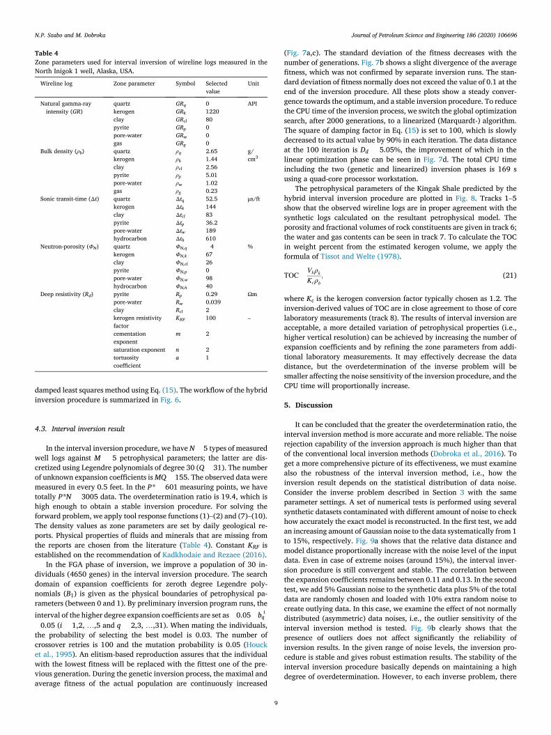
In the interval inversion procedure, we have N ¼ 5 types of measured well logs against M ¼ 5 petrophysical parameters; the latter are dis-cretized using Legendre polynomials of degree 30 (Q ¼ 31). The number of unknown expansion coefficients is MQ ¼ 155. The observed data were measured in every 0.5 feet. In the P* ¼ 601 measuring points, we have totally P*N ¼ 3005 data. The overdetermination ratio is 19.4, which is high enough to obtain a stable inversion procedure. For solving the forward problem, we apply tool response functions (1)–(2) and (7)–(10). The density values as zone parameters are set by daily geological re-ports. Physical properties of fluids and minerals that are missing from the reports are chosen from the literature (Table 4). Constant KRF is established on the recommendation of Kadkhodaie and Rezaee (2016).

In the FGA phase of inversion, we improve a population of 30 in-dividuals (4650 genes) in the interval inversion procedure. The search domain of expansion coefficients for zeroth degree Legendre poly-nomials (B1) is given as the physical boundaries of petrophysical pa-rameters (between 0 and 1). By preliminary inversion program runs, the interval of the higher degree expansion coefficients are set as � 0.05� bðiÞq

�0.05 (i ¼ 1,2, …,5 and q ¼ 2,3, …,31). When mating the individuals, the probability of selecting the best model is 0.03. The number of crossover retries is 100 and the mutation probability is 0.05 (Houck et al., 1995). An elitism-based reproduction assures that the individual with the lowest fitness will be replaced with the fittest one of the pre-vious generation. During the genetic inversion process, the maximal and average fitness of the actual population are continuously increased

(Fig. 7a,c). The standard deviation of the fitness decreases with the number of generations. Fig. 7b shows a slight divergence of the average fitness, which was not confirmed by separate inversion runs. The stan-dard deviation of fitness normally does not exceed the value of 0.1 at the end of the inversion procedure. All these plots show a steady conver-gence towards the optimum, and a stable inversion procedure. To reduce the CPU time of the inversion process, we switch the global optimization search, after 2000 generations, to a linearized (Marquardt-) algorithm. The square of damping factor in Eq. (15) is set to 100, which is slowly decreased to its actual value by 90% in each iteration. The data distance at the 100 iteration is Dd ¼ 5.05%, the improvement of which in the linear optimization phase can be seen in Fig. 7d. The total CPU time including the two (genetic and linearized) inversion phases is 169 s using a quad-core processor workstation.

The petrophysical parameters of the Kingak Shale predicted by the hybrid interval inversion procedure are plotted in Fig. 8. Tracks 1–5 show that the observed wireline logs are in proper agreement with the synthetic logs calculated on the resultant petrophysical model. The porosity and fractional volumes of rock constituents are given in track 6; the water and gas contents can be seen in track 7. To calculate the TOC in weight percent from the estimated kerogen volume, we apply the formula of Tissot and Welte (1978).

TOC¼Vkρk

Kcρb; (21)

where Kc is the kerogen conversion factor typically chosen as 1.2. The inversion-derived values of TOC are in close agreement to those of core laboratory measurements (track 8). The results of interval inversion are acceptable, a more detailed variation of petrophysical properties (i.e., higher vertical resolution) can be achieved by increasing the number of expansion coefficients and by refining the zone parameters from addi-tional laboratory measurements. It may effectively decrease the data distance, but the overdetermination of the inverse problem will be smaller affecting the noise sensitivity of the inversion procedure, and the CPU time will proportionally increase.

5. Discussion

It can be concluded that the greater the overdetermination ratio, the interval inversion method is more accurate and more reliable. The noise rejection capability of the inversion approach is much higher than that of the conventional local inversion methods (Dobr�oka et al., 2016). To get a more comprehensive picture of its effectiveness, we must examine also the robustness of the interval inversion method, i.e., how the inversion result depends on the statistical distribution of data noise. Consider the inverse problem described in Section 3 with the same parameter settings. A set of numerical tests is performed using several synthetic datasets contaminated with different amount of noise to check how accurately the exact model is reconstructed. In the first test, we add an increasing amount of Gaussian noise to the data systematically from 1 to 15%, respectively. Fig. 9a shows that the relative data distance and model distance proportionally increase with the noise level of the input data. Even in case of extreme noises (around 15%), the interval inver-sion procedure is still convergent and stable. The correlation between the expansion coefficients remains between 0.11 and 0.13. In the second test, we add 5% Gaussian noise to the synthetic data plus 5% of the total data are randomly chosen and loaded with 10% extra random noise to create outlying data. In this case, we examine the effect of not normally distributed (asymmetric) data noises, i.e., the outlier sensitivity of the interval inversion method is tested. Fig. 9b clearly shows that the presence of outliers does not affect significantly the reliability of inversion results. In the given range of noise levels, the inversion pro-cedure is stable and gives robust estimation results. The stability of the interval inversion procedure basically depends on maintaining a high degree of overdetermination. However, to each inverse problem, there

Table 4 Zone parameters used for interval inversion of wireline logs measured in the North Inigok 1 well, Alaska, USA.

Wireline log Zone parameter Symbol Selected value

Unit

Natural gamma-ray intensity (GR)

quartz GRq 0 API kerogen GRk 1220 clay GRcl 80 pyrite GRp 0 pore-water GRw 0 gas GRg 0

Bulk density (ρb) quartz ρq 2.65 g/ cm3 kerogen ρk 1.44

clay ρcl 2.56 pyrite ρp 5.01 pore-water ρw 1.02 gas ρg 0.23

Sonic transit-time (Δt) quartz Δtq 52.5 μs/ft kerogen Δtk 144 clay Δtcl 83 pyrite Δtp 36.2 pore-water Δtw 189 hydrocarbon Δth 610

Neutron-porosity (ΦN) quartz ΦN,q � 4 % kerogen ΦN,k 67 clay ΦN,cl 26 pyrite ΦN,p 0 pore-water ΦN,w 98 hydrocarbon ΦN,h 40

Deep resistivity (Rd) pyrite Rp 0.29 Ωm pore-water Rw 0.039 clay Rcl 2 kerogen resistivity factor

KRF 100 –

cementation exponent

m 2

saturation exponent n 2 tortuosity coefficient

a 1

N.P. Szab�o and M. Dobr�oka

Journal of Petroleum Science and Engineering 186 (2020) 106696

10

exist an optimal number of expansion coefficients for each model parameter. An automated solution to specify the number of coefficients was published by Dobr�oka et al. (2016), which is based on the mini-mization of average correlation between the inversion unknowns. The selected number of coefficients should be also affected by the length of the processing interval, inhomogeneity of the formation etc. Generally speaking, a trade-off must be made between the number of unknowns

and the accuracy (and vertical resolution) we want to achieve by the use of the inversion approach.

The FGA search assures to find a global maximum of the fitness function, which can be verified by running the inversion procedure for several times using the same dataset. We randomly generate 30 vectors of series expansion coefficients, which are improved over 2000 gener-ations by the genetic inversion procedure. After the evolutionary phase,

Fig. 7. Convergence to the optimum during the genetic (a–c) and linear (d) optimization phases of the interval inversion procedure.

Fig. 8. Result of the combined interval inversion procedure, North Inigok 1 well, Alaska, USA.

N.P. Szab�o and M. Dobr�oka

Journal of Petroleum Science and Engineering 186 (2020) 106696

11

Fig. 9. Noise rejection test results for normally distributed (a) and non-Gaussian (outlier-rich) (b) data noise.

Fig. 10. Frequency plots showing the impact of random initialization of genetic algorithm (a–c) on the interval inversion result (d) in North Inigok 1 well, Alaska, USA.

N.P. Szab�o and M. Dobr�oka

Journal of Petroleum Science and Engineering 186 (2020) 106696

12

we switch to linear optimization to give a final solution to the inverse problem (Fig. 6). To measure the impact of random initialization of FGA on the interval inversion result, we run the inversion procedure 20 times with the same parameter settings using the well logging dataset of North Inigok 1 well (Section 4). In Fig. 10a� c, the histograms refer to the re-sults of 20 independent inversion runs. All the three plots show that a very heterogeneous distribution of random models are present in the initial population. The minimum of the average fitness of individuals corresponds to a data distance of Dd~104% according to Eq. (18), while the mean of the maximal fitness is F ¼ � 27.2. At the end of each inversion runs, we calculate the data distance of the inversion result, respectively. The average of data distances is Dd ¼ 5.16% with a stan-dard deviation of 0.36%, which show consistent results. Further improvement of these inversion results can be made by increasing the number of iterations of the genetic inversion process (the same global optimum could be only reached by using a purely FGA assisted interval inversion method), and by revising the petrophysical model and theo-retical response functions.

6. Conclusions

The interval inversion method is presented as new alternative tool for evaluating unconventional hydrocarbon formations. A large data-to- unknowns ratio of the inverse problem assures very stable inversion procedure and makes it possible to estimate several petrophysical pa-rameters of organic-rich reservoirs with high accuracy and reliability. A robust behavior of the suggested inversion method is also observable, which allows the processing of erroneous or old well logs having outlying values. We also experience that even higher number of petro-physical properties (not expansion coefficients) than data types can be reliably treated by the interval inversion method, without the problem of ambiguity. For instance, more unknowns can be added to the inver-sion procedure such as the fractional volumes of different clay types (dry or wet), feldspars, dolomite, heavy minerals, and bounded water and gas contents etc. As in earlier applications, some zone parameters to which the observed well logs are sensitive enough can be automatically extracted by inversion. In organic rich formations, the objective deter-mination of the physical properties of kerogen or LOM is of great importance. The kerogen volume can be very accurately estimated by interval inversion, which helps better separating and analyzing the sweet spots in source rocks. The performance of the proposed inversion method can be improved by the further development of the forward problem. The tool response equations must be revisited, for instance the water saturation will be estimated better, e.g., by taking the role of absorbed gas content into consideration in resistivity modeling. For a more detailed analysis, one can divide a long processing interval into smaller segments, in all of which high degree polynomials gives proper vertical resolution. In reservoirs of large areal extent, the multi-well implementation of the interval inversion method is recommended, which is able to follow the lateral variation of shale formations with high TOC contents. As a modern approach, all of the above problems can be solved by an adaptive genetic algorithm optimization strategy to make the interval inversion method a robust tool for the exploration of un-conventional petroleum resources.

Acknowledgments

The research was supported by the GINOP-2.3.2-15-2016-00010 “Development of enhanced engineering methods with the aim at utili-zation of subterranean energy resources” project in the framework of the Sz�echenyi 2020 Plan, funded by the European Union, co-financed by the European Structural and Investment Funds. The authors thank to Wil-liam Rouse and David Houseknecht from U. S. Geological Survey for providing field data for the study. The first author addresses special thanks to his father B�ela Szab�o (1950–2019), who gave his loving care, support and kind attention throughout his life.

Appendix A. Supplementary data

Supplementary data to this article can be found online at https://doi. org/10.1016/j.petrol.2019.106696.

References

Alberty, M., Hashmy, K., 1984. Application of ULTRA to log analysis. SPWLA 25th annual logging symposium. SPWLA-1984-Z 1–17.

Aleardi, M., 2019. Using orthogonal Legendre polynomials to parameterize global geophysical optimizations: applications to seismic-petrophysical inversion and 1D elastic full-waveform inversion. Geophys. Prospect. 67 (2), 331–348.

Baker Atlas, 1996. OPTIMA: eXpress Reference Manual, Baker Atlas. Western Atlas International, Inc.

Bibor, I., Szab�o, N.P., 2016. Unconventional shale characterization using improved well logging methods. Geosci. Eng. 5 (8), 32–50.

Carpentier, B., Huc, A., Bessereau, G., 1991. Wireline logging and source rocks - estimation of organic carbon content by the CARBOLOG method. Log. Anal. 32, 279–297.

Crain, E.R., 2019. Crain’s Petrophysical Handbook. online at. P. Eng. www.spec2000.net. Dobr�oka, M., Szab�o, N.P., 2011. Interval inversion of well-logging data for objective

determination of textural parameters. Acta Geophys. 59, 907–934. Dobr�oka, M., Szab�o, N.P., 2012. Interval inversion of well-logging data for automatic

determination of formation boundaries by using a float-encoded genetic algorithm. J. Pet. Sci. Eng. 86–87, 144–152.

Dobr�oka, M., Szab�o, P.N., Cardarelli, E., Vass, P., 2009. 2D inversion of borehole logging data for simultaneous determination of rock interfaces and petrophysical parameters. Acta Geod. Geophys. Hung. 44, 459–479.

Dobr�oka, M., Szab�o, N.P., Turai, E., 2012. Interval inversion of borehole data for petrophysical characterization of complex reservoirs. Acta Geod. Geophys. Hung. 47, 172–184.

Dobr�oka, M., Szab�o, N.P., T�oth, J., Vass, P., 2016. Interval inversion approach for an improved interpretation of well logs. Geophysics 81, D155–D167.

Drahos, D., 1984. Electrical modeling of the inhomogeneous invaded zone. Geophysics 49, 1580–1585.

Horv�ath, Sz, B, 1973. The accuracy of petrophysical parameters as derived by computer processing. Log. Anal. 14, 16–33.

Houck, C.R., Joines, J., Kay, M., 1995. A Genetic Algorithm for Function Optimization: A Matlab Implementation. NCSU-IE Technical Report 95� 09. North Carolina State University, pp. 1–14.

Houseknecht, D.W., Bird, K.J., 2004. Sequence stratigraphy of the Kingak shale (Jurassic–Lower cretaceous), national petroleum reserve in Alaska. AAPG (Am. Assoc. Pet. Geol.) Bull. 88 (3), 279–302.

Jarzyna, J.A., Cichy, A., Drahos, D., Galsa, A., Bala, M.J., Ossowski, A., 2016. New methods for modeling laterolog resistivity corrections. Acta Geophys. 64 (2), 417–442.

Kadkhodaie, A., Rezaee, R., 2016. A new correlation for water saturation calculation in gas shale reservoirs based on compensation of kerogen-clay conductivity. J. Pet. Sci. Eng. 146, 932–939.

Ma, Z., Holditch, S., 2015. Unconventional Oil and Gas Resources Handbook: Evaluation and Development. Elsevier/Gulf Professional Publishing.

Marquardt, D.W., 1959. Solution of non-linear chemical engineering models. Chem. Eng. Prog. 55, 65–70.

Mayer, C., Sibbit, A.M., 1980. GLOBAL, a new approach to computer-processed log interpretation. In: Proceedings of the 55th SPE Annual Fall Technical Conference and Exhibition, Paper, vol. 9341, pp. 1–14.

Menke, W., 1984. Geophysical Data Analysis: Discrete Inverse Theory. Academic Press. Michalski, A., 2013. Global Optimization: Theory, Developments and Applications. Nova

Publishers. Michalewicz, Z., 1992. Genetic Algorithms þ Data Structures ¼ Evolution Programs.

Springer. Naeini, E.Z., Green, S., Rauch-Davies, M., 2019. An integrated deep learning solution for

petrophysics, pore pressure, and geomechanics property prediction. Lead. Edge 38, 53–59.

Passey, Q., Creaney, S., Kulla, J., Moretti, F., Stroud, J., 1990. A practical model for organic richness from porosity and resistivity logs. Am. Assoc. Petrol. Geol. Bull. 74 (12), 1777–1794.

Poupon, A., Leveaux, J., 1971. Evaluation of water saturation in shaly formations. In: Transactions SPWLA 12th Annual Logging Symposium, SPWLA-1971-vXIIn4a1, pp. 1–2.

Puskarczyk, E., Jarzyna, J.A., Wawrzyniak-Guz, K., Krakowska, P.I., Zych, M., 2019. Improved recognition of rock formation on the basis of well logging and laboratory experiments results using factor analysis. Acta Geophys. 1–14 (in press).

Raymer, L.L., Hunt, E.R., Gardner, J.S., 1980. An improved sonic transit time-to-porosity transform. In: SPWLA 21st Annual Logging Symposium. SPWLA-1980-P, pp. 1–12.

Renchun, H., Yan, W., Sijie, C., Shuai, L., Li, C., 2015. Selection of logging-based TOC calculation methods for shale reservoirs: a case study of the Jiaoshiba shale gas field in the Sichuan Basin. Nat. Gas. Ind. B 2 (2–3), 155–161.

Rouse, W.A., Houseknecht, D.W., 2016. Modified Method for Estimating Petroleum Source-Rock Potential Using Wireline Logs, with Application to the Kingak Shale, Alaska North Slope, vols. 2016–5001. U.S. Geological Survey Scientific Investigations Report, p. 40.

Schlumberger, 1989. Log Interpretation Principles/applications. Seventh printing, Schlumberger.

N.P. Szab�o and M. Dobr�oka

Journal of Petroleum Science and Engineering 186 (2020) 106696

13

Schmoker, J.W., 1979. Determination of organic content of Appalachian Devonian shales from formation-density logs. Am. Assoc. Petrol. Geol. Bull. 63 (9), 1504–1537.

Simandoux, P., 1963. Dielectric measurements in porous media and application to shaly formation. Rev. Inst. Fr. Pet. 18, 193–215.

Sondergeld, C.H., Newsham, K.E., Comisky, J.T., Rice, M.C., Rai, C.S., 2010. Petrophysical considerations in evaluating and producing shale gas resources. In: SPE Unconventional Gas Conference, 131768-MS.

Szab�o, N.P., Dobr�oka, M., 2018. Exploratory factor analysis of wireline logs using a Float- Encoded Genetic Algorithm. Math. Geosci. 50 (3), 317–335.

Szab�o, N.P., Dobr�oka, M., 2019. Series expansion-based genetic inversion of wireline logging data. Math. Geosci. 51 (6), 811–835.

Szab�o, N.P., 2018. A genetic meta-algorithm-assisted inversion approach: hydrogeological study for the determination of volumetric rock properties and

matrix and fluid parameters in unsaturated formations. Hydrogeol. J. 26 (6), 1935–1946.

Tissot, B.P., Welte, D.H., 1978. Petroleum Formation and Occurrence. Springer. Wang, P., Chen, Z., Pang, X., Hu, K., Sun, M., Chen, X., 2015. Revised models for

determining TOC in shale play: example from devonian duvernay shale, western Canada sedimentary basin. Mar. Pet. Geol. 70, 304–319.

Wyllie, M.R.J., Gregory, A.R., Gardner, L.W., 1956. Elastic wave velocities in heterogeneous and porous media. Geophysics 21, 41–70.

Xu, J., Xu, L., Qin, Y., 2017. Two effective methods for calculating water saturations in shale gas reservoirs. Geophysics 82 (3), D187–D197.

Zhao, P., Mao, Z., Huang, Z., Zhang, C., 2016. A new method for estimating total organic carbon content from well logs. AAPG (Am. Assoc. Pet. Geol.) Bull. 100 (8), 1311–1327.

N.P. Szab�o and M. Dobr�oka