Weighted skewness and kurtosis unbiased by sample size - arXiv · Weighted skewness and kurtosis...

Weighted skewness and kurtosisunbiased by sample size

Lorenzo Rimoldini

Observatoire astronomique de l’Universite de Geneve, chemin des Maillettes 51, CH-1290 Versoix, SwitzerlandISDC Data Centre for Astrophysics, Universite de Geneve, chemin d’Ecogia 16, CH-1290 Versoix, Switzerland

[email protected]

Draft version: April 28, 2013

Abstract

Central moments and cumulants are often employed to characterize the distribution ofdata. The skewness and kurtosis are particularly useful for the detection of outliers, theassessment of departures from normally distributed data, automated classification tech-niques and other applications. Robust definitions of higher order moments are more stablebut might miss characteristic features of the data, as in the case of astronomical time serieswith rare events like stellar bursts or eclipses from binary systems. Weighting can helpidentify reliable measurements from uncertain or spurious outliers, so unbiased estimatesof the weighted skewness and kurtosis moments and cumulants, corrected for sample-sizebiases, are provided under the assumption of independent data. The comparison of biasedand unbiased weighted estimators is illustrated with simulations as a function of samplesize, employing different data distributions and weighting schemes.

1 IntroductionDescriptive statistics provide essential tools to quantify the main features of data and typically consistof simple quantities which can be computed efficiently and easily included in the analysis of large datavolumes. The ability to summarize essential information in a few parameters has found widespread inter-disciplinary applications. Central moments characterize the shape of the distribution of measurementsaround the mean value for most distributions occurring in practice. The familiar moments of variance,skewness and kurtosis give indications on the dispersion, asymmetry and peakedness or weight of thetails of the distribution, respectively.

Moments are usually computed on random variables. Herein, their application is extended to datagenerated from deterministic functions and randomized by the uneven sampling of a finite number ofmeasurements and by their uncertainties, whereas the corresponding ‘population’ statistics are defined inthe limit of an infinite regular sampling with no random or systematic errors. This scenario is common inastronomical time series, where measurements are typically non-regular due to observational constraints,they are unavoidably affected by noise and sometimes also not very numerous: all of these aspectsintroduce some level of randomness in the characterization of the underlying signal of a star.

While the effects of noise and sampling on time series are studied in Rimoldini (2013a,b), this workaddresses the bias, precision and accuracy of weighted estimators in the case of small sample sizes. Biasis defined as the difference between expectation and population values and thus expresses a systematicdeviation from the true value. Precision is described by the dispersion of measurements, while accuracyis related to the distance of an estimator from the true value and thus combines the bias and precisionconcepts (e.g., accuracy can be measured by the mean square error, defined by the sum of bias anduncertainty in quadrature).

Higher moments such as skewness and kurtosis have received particular attention for the detection ofoutliers and of departures from normally distributed data (D’Agostino, 1986). The underlying conceptscan be expressed in many alternative ways, some of which (e.g., Moors et al., 1996; Hosking, 1990;

Weighted skewness and kurtosis unbiased by sample size page 1 of 33

arX

iv:1

304.

6564

v2 [

astr

o-ph

.IM

] 2

8 A

pr 2

013

Groeneveld & Meeden, 1984; Bowley, 1920) avoid sample means or non-linear transformations and favourmore robust results. While insensitivity to a few botched measurements is a clear advantage, sometimesoutliers are part of the targeted signal, as in the case of eclipses occurring in the light curves of binarystar systems. Since weighting can help distinguish meaningful outliers (e.g., the data corresponding toeclipsed phases) from spurious measurements, the present work focusses on the conventional definitionsof skewness and kurtosis in terms of central moments and cumulants, and provides sample-size corrected(‘unbiased’) estimates of the weighted formulations.

Sample moments do not provide unbiased estimates of population moments. As the sample sizedecreases, the uncertainty of the sample mean around the population value increases and higher ordercentral moments can become biased as a result. Statistical estimators which remain unbiased as a functionof sample size are relevant to those applications which aim at the characterization of the populationwhich the measured sample represents. This approach is particularly important for the interpretationand comparison of data in a broader context than the sole description of a sample.

Weighting can quantify the relevance of measurements (e.g., by inverse-squared uncertainties), enhancetargeted features of the data depending on the objectives of the analysis, and have different implicationson the precision and accuracy of estimators:

(i) They might decrease, because weights assign more importance to some data at the expense of otherones, effectively reducing the sample size as results depend mostly on fewer ‘relevant’ measurements.This case is apparent in Sec. 5, for example, when weighting by the inverse-squared uncertaintiesat high signal-to-noise (S/N) ratios.

(ii) They might increase, when weights reduce greater dispersions and biases than the ones caused byan effectively smaller sample. For example, weighting by inverse-squared uncertainties was shownto improve both precision and accuracy at low S/N levels (Rimoldini, 2013a).

Weighting might exploit correlations in the data to improve precision (Rimoldini, 2013b). Since correlateddata do not satisfy the assumptions of the expressions derived herein, their application might returnbiased results. However, small biases could be justified if improvements in precision are significant and,depending on the extent of the application, larger biases could be mitigated with mixed weighting schemes,such as the one described in Sec. 5.

Similarly to the pros and cons of weighting, unbiased estimators are expected to be more accuratebut less precise than the biased counterparts, since they take into account the uncertainty of the samplemean. Thus, they are favoured when biases from small sample sizes are larger than the dispersion ofunbiased statistics. A compromise solution (weighted or unweighted, biased or unbiased) should balancebiases against the dispersion of weighted or unbiased estimators (which might depend on the statisticsand the data), improve the overall accuracy and be applied uniformly to all data.

Unbiased expressions are derived for the weighted skewness and kurtosis (central moments and cu-mulants) in the case of independent measurements. The results are illustrated with simulated data andthe dependence of unbiased weighted estimators on sample size is shown for two weighting schemes: thecommon inverse-squared uncertainties and interpolation-based weights as described in Rimoldini (2013b).The latter demonstrated a significant improvement in the precision of weighted moments and cumulantsfor data sets with at least a few tens of measurements.

This paper is organized as follows. The notation employed throughout is defined in Sec. 2. Sample(biased) weighted moments and cumulants are recalled in Sec. 3. Sample-size unbiased weighted andunweighted moments and cumulants are presented in Sec. 4. Biased and unbiased estimators are comparedwith simulated signals as a function of sample size in Sec. 5, including weighted and unweighted estimatorsand two different signal shapes. Conclusions are drawn in Sec. 6, followed by detailed derivations of thesample-size unbiased weighted estimators in App. A.


2 Notation

For a set of n measurements x = (x1, x2, ..., xn), the following quantities are defined.

(i) Population central moments µr=E[(x−µ)r] with mean µ = E(x), where E(.) denotes expectation,and cumulants κ2 = µ2, κ3 = µ3, κ4 = µ4 − 3µ2

2 (e.g., Stuart & Ord, 1969).1

(ii) The sum of the p-th power of weights is defined as Vp =∑ni=1 w

pi .

(iii) Sample central moments mr =∑ni=1 wi(xi − x)r/V1 and corresponding cumulants kr.

(iv) Sample-size unbiased estimates of central moments Mi and cumulants Ki, i.e., E(Mi) = µi andE(Ki) = κi.

(v) The standardized skewness and kurtosis are defined as g1 = k3/k3/22 , g2 = k4/k

22, G1 = K3/K

3/22 ,

and G2 = K4/K22 , with population values γ1 = κ3/κ

3/22 and γ2 = κ4/κ

22. G1 and G2 satisfy

consistency (for n→∞) but are not unbiased in general (e.g., see Heijmans, 1999, for exceptions).

(vi) No systematics or other instrumental errors are considered herein and uncertainties are often referredto as errors.

(vii) Statistics weighted by the inverse-squared uncertainties are called ‘error-weighted’ for brevity andinterpolation-based weights computed in phase (Rimoldini, 2013b) are named ‘phase weights’.

3 Sample moments and cumulantsThe sample weighted central moments, such as the variance m2, skewness m3, kurtosis m4 and therespective cumulants, are defined in terms of the weighted mean x as follows:

x =1

V1

n∑i=1

wixi (1)

m2 =1

V1

n∑i=1

wi(xi − x)2 = k2 (2)

m3 =1

V1

n∑i=1

wi(xi − x)3 = k3 (3)

m4 =1

V1

n∑i=1

wi(xi − x)4 (4)

k4 = m4 − 3m22. (5)

The unweighted forms can be obtained by substituting wi = 1 (for all i) and V1 = n in the aboveequations.

1Cumulants, first derived by Thiele (1889), have also been named ‘cumulative moment functions’ (Fisher, 1929) and‘semi-invariants’ by other authors (e.g., Cramer, 1961; Dressel, 1940).


4 Sample-size unbiased moments and cumulantsThe sample-size bias corrected weighted central moments, such as the variance M2, skewness M3, kur-tosis M4 and the respective cumulants are derived assuming independent measurements and weights, asdescribed in full detail in App. A. They are defined in terms of sample estimators as follows:

M2 =V 21

V 21 − V2

m2 = K2 (6)

M3 =V 31

V 31 − 3V1V2 + 2V3

m3 = K3 (7)

M4 =V 21 (V 4

1 − 3V 21 V2 + 2V1V3 + 3V 2

2 − 3V4)

(V 21 − V2)(V 4

1 − 6V 21 V2 + 8V1V3 + 3V 2

2 − 6V4)m4 +

− 3V 21 (2V 2

1 V2 − 2V1V3 − 3V 22 + 3V4)

(V 21 − V2)(V 4

1 − 6V 21 V2 + 8V1V3 + 3V 2

2 − 6V4)m2

2 (8)

K4 =V 21 (V 4

1 − 4V1V3 + 3V 22 )

(V 21 − V2)(V 4

1 − 6V 21 V2 + 8V1V3 + 3V 2

2 − 6V4)m4 +

− 3V 21 (V 4

1 − 2V 21 V2 + 4V1V3 − 3V 2

2 )

(V 21 − V2)(V 4

1 − 6V 21 V2 + 8V1V3 + 3V 2

2 − 6V4)m2

2 . (9)

The corresponding unweighted forms can be achieved by direct substitution Vp = n for all p, leadingto the known relations (e.g., see Cramer, 1961):

M2 =n

n− 1m2 = K2 (10)

M3 =n2

(n− 1)(n− 2)m3 = K3 (11)

M4 =n(n2 − 2n+ 3)

(n− 1)(n− 2)(n− 3)m4 −

3n(2n− 3)

(n− 1)(n− 2)(n− 3)m2

2 (12)

K4 =n2(n+ 1)

(n− 1)(n− 2)(n− 3)m4 −

3n2

(n− 2)(n− 3)m2

2. (13)

5 Estimators as a function of sample sizeThe effect of different weighting schemes on sample and population estimators is illustrated as a function ofsample size with simulated data, through which biased and unbiased estimators are compared for specificperiodic signals, sampling and error laws. The values of the population moments of the continuoussimulated periodic ‘true’ signal ξ(φ) are computed averaging in phase φ as follows:

µr =1

2π

∫ 2π

0

[ξ(φ)− µ]r

dφ, where µ =1

2π

∫ 2π

0

ξ(φ) dφ. (14)

5.1 Simulation

Simulated signals are described by a simple sinusoidal function to the first and the fourth powers. Thesignal ξ(φ) with variance µ2 and signal-to-noise ratio S/N (estimated by the ratio of the standard devi-ation

√µ2 and the root of the mean of squared measurement uncertainties εi) is sampled from n = 10 to

1000 times at phases φi randomly drawn from a uniform distribution:ξ(φ) = ξo +A sinα φ

xi ∼ N (ξi, ε2i ) for ξi = ξ(φi) and φi ∼ U(0, 2π)

ε2i = (1 + ρi) µ2 / (S/N)2 for ρi ∼ U(−0.8, 0.8),

(15)

(16)

(17)


0.0 0.2 0.4 0.6 0.8 1.0

−1.

0−

0.5

0.0

0.5

1.0

Phase (φ / 2π)

Sig

nal a

nd s

imul

ated

dat

a

●●●●

●●

●●●●

●● ●●●●●●

●

●

●●●

●●

●

●

●●●

●●●

●●●●●●●●●

●

●

●

●

●●

●●

S/N = 100, n = 50

●●●●

●●

●●●●

●● ●●●●●●

●

●

●●●

●●

●

●

●●●

●●●

●●●●●●●●●

●

●

●

●

●●

●●

sin4φsin φ

Figure 1: Simulated signals of the forms of sin4 φ (solid blue curve) and sinφ (dashed red curve) areirregularly sampled by 50 measurements (denoted by blue triangles and red circles, respectively) withS/N = 100.

Table 1: Population values of the estimators illustrated in Figs 2–16.

Population Equivalent Population values for ξ(φ) = ξo +A sinα φ

Statistics Expression α = 1 α = 4

µ – ξo ξo + 3A/8

µ2 κ2 A2/2 17A2/128

µ3 κ3 0 3A3/128

µ4 κ4 + 3κ22 3A4/8 963A4/32768

κ4 µ4 − 3µ22 −3A4/8 −771A4/32768

γ1 κ3/κ3/22 , µ3/µ

3/22 0

√1152/4913 ≈ 0.484

γ2 κ4/κ22, µ4/µ

22 − 3 −3/2 −771/578 ≈ −1.334

where α = 1, 4 and the i-th measurement xi is drawn from a normal distribution N (ξi, ε2i ) of mean ξi and

variance ε2i . The latter is defined in terms of a variable ρi randomly drawn from a uniform distributionU(−0.8, 0.8) so that measurement uncertainties vary by up to a factor of 3 for a given µ2 and S/N ratio.Simulations were repeated 104 times for each sample size.

The dependence of estimators on noise and the corresponding unbiased expressions were presented inRimoldini (2013a). Herein, the S/N ratio is set to 100 so that noise biases are negligible with respect tothe ones resulting from small sample sizes. Sample signals and simulated data are illustrated in Fig. 1 forn = 50. The reference population values of the mean, variance, skewness and kurtosis of the simulatedsignals are listed in Table 1.


Error weights are defined by wi = 1/ε2i , while phase weights follow Rimoldini (2013b), assumingphase-sorted data:

wi = h(n|a, b) w′i∑nj=1 w

′j

+ [1− h(n|a, b)] /n ∀i ∈ (1, n)

w′i = φi+1 − φi−1 ∀i ∈ (2, n− 1)

w′1 = φ2 − φn + 2π

w′n = φ1 − φn−1 + 2π

h(n|a, b) =1

1 + e−(n−a)/bfor a, b > 0.

(18)

(19)

(20)

(21)

(22)

Estimators derived herein assume a single weighting scheme and combinations of estimators (like thevariance and the mean in the standardized skewness and kurtosis) are expected to apply the same weightsto terms associated with the same measurements. The function h(n|a, b) constitutes just an example toachieve a mixed weighting scheme: tuning parameters a, b offer the possibility to control the transitionfrom unweighted to phase-weighted estimators (in the limits of small and large n, respectively) and thusreach a compromise solution between precision and accuracy for all values of n, according to the specificestimators, signals, sampling, errors, sample sizes and their distributions in the data.

5.2 Results

Figure 2 illustrates the sample mean in the various scenarios considered in the simulations at S/N = 100:unweighted and with different weighting schemes (error-weighted and phase-weighted). While accuracyis the same in all cases, the best precision of the mean is achieved employing phase weights, with no needto limit interpolation within large gaps for small sample sizes.

Figures 3–16 compare biased and unbiased estimators as a function of sample size, evaluating thefollowing deviations from the population values:

M2/µ2 − 1 vs m2/µ2 − 1, (23)

M3/µ3/22 − γ1 vs m3/µ

3/22 − γ1, G1 − γ1 vs g1 − γ1, (24)

M4/µ22 − 3− γ2 vs m4/µ

22 − 3− γ2, M4/M

22 − 3− γ2 vs m4/m

22 − 3− γ2, (25)

K4/µ22 − γ2 vs k4/µ

22 − γ2, G2 − γ2 vs g2 − γ2, (26)

in both weighted and unweighted cases, for signals of the forms sinφ and sin4 φ, with S/N = 100.Estimators standardized by both true and estimated variance are presented to help interpret the behaviourof the ratios from their components.

Biased and unbiased estimators are quite similar in the limit of large sample sizes (typically n > 100).When weighting by errors, or not weighting at all, unbiased estimators are accurate throughout the wholerange of sample sizes, as expected, although their precision decreases at lower values of n. The biasedcounterparts are more precise but less accurate, with a degradation of both accuracy and precision atlow n.

Estimators which involve ratios (and powers) of unbiased estimators are not expected to be unbiasedin general. Figures 5–8 and 13–16 show that the ratios g1, g2 of sample estimators (weighted or not) aremore precise and accurate than the ratios G1, G2 of the respective unbiased counterparts.

Weighting by phase intervals leads to a significant improvement in precision of all estimators in thelimit of large sample sizes n and a reduction of accuracy of many ‘unbiased’ estimators at low n, becauseof the introduction of correlations through phase weights (as the closer measurements are in phase, themore similar their values are likely to be; see Rimoldini, 2013b). Tuning parameters such as a = 25and b = 6 in Eq. (18) have shown to be able to mitigate the inaccuracy of unbiased estimators at low nand reduce to the unweighted results, which appear to be the most accurate and precise in the limit ofsmall sample sizes (in these simulations). This solution might provide a reasonable compromise betweenprecision and accuracy of unbiased estimators, at least for sample sizes n > 10.


Estimators of sinusoidal signals appeared more precise than those arising from the fourth power of asine, with the exception of the mean, for which the relative precision of the two signal shapes reversed inmost cases.

From the comparison of sample-size biased and unbiased estimators with different weighting schemesfor the two periodic signals considered, it appears that, at high S/N ratios, sample-size biased phase-weighted estimators (with a, b→ 0) have the best precision and accuracy in general, with the exception ofm2, m3 and m4/m2, which become biased especially for n < 20. Further improvements might be achievedby tuning parameters better fitted to estimators and signals of interest, in view of specific requirementsof precision and accuracy.

6 ConclusionsExact expressions of weighted skewness and kurtosis corrected for sample-size biases are provided inEqs (7)–(9) under the assumption of independent measurements and weights. Such estimators are par-ticularly useful when the adoption of a weighting scheme is important for the processing of the data andaccuracy needs to be preserved at small sample sizes.

Simulations of irregularly sampled symmetric and skewed periodic signals were employed to comparesample-size biased and unbiased estimators as a function of sample size in the unweighted, inverse-squarederror weighted and phase-interval weighted schemes. While phase weighting introduced correlations (notconsidered by the unbiased weighted expressions), a mixed phase and error weighting scheme was able tobalance precision and accuracy on a wide range of sample sizes.

AcknowledgmentsThe author thanks M. Suveges for many discussions and valuable comments on the original manuscript.

ReferencesBowley A.L., 1920, Elements of Statistics, Charles Scribner’s Sons, New York

Cramer H., 1961, Mathematical Methods of Statistics, Princeton University Press

D’Agostino R.B., 1986, Goodness-of-fit techniques, D’Agostino & Stephens eds., Marcel Dekker, NewYork, p. 367

Dressel P.L., 1940, Annals of Mathematical Statistics, 11, 33

Fisher R.A., 1929, Proceedings of the London Mathematical Society, Series 2, 30, 199

Groeneveld R.A., Meeden G., 1984, The Statistician, 33, 391

Heijmans R., 1999, Statistical Papers, 40, 107

Hosking J.R.M., 1990, J. R. Statist. Soc. B, 52, 105

Moors J.J.A., Wagemakers R.Th.A., Coenen V.M.J., Heuts R.M.J., Janssens M.J.B.T., 1996, StatisticaNeerlandica, 50, 417

Rimoldini L., 2013a, preprint (arXiv:1304.6715)

Rimoldini L., 2013b, preprint (arXiv:1304.6616)

Stuart A., Ord J., 1969, Kendall’s Advanced Theory of Statistics, Charles Griffin & Co. Ltd, London

Thiele T.N., 1889, Forlaesinger over almindelig iagttagelseslaere: sandsynlighedsregning og mindstekvadraters methode, C.A. Reitzel, Copenhagen


http://xxx.lanl.gov/abs/1304.6715

http://xxx.lanl.gov/abs/1304.6616

Mean(sinφ, sin4 φ)

Unweighted

−0.4

−0.2

0.0

0.2

0.4

0.00 0.02 0.04 0.06 0.08 0.10

(Sample size)−1

mea

n −

µ

sin

sin^4

Phase Weighted (a, b→ 0)

−0.4

−0.2

0.0

0.2

0.4

0.00 0.02 0.04 0.06 0.08 0.10

(Sample size)−1

mea

n −

µ

sin

sin^4

Error Weighted

−0.4

−0.2

0.0

0.2

0.4

0.00 0.02 0.04 0.06 0.08 0.10

(Sample size)−1

mea

n −

µ

sin

sin^4

Phase Weighted (a = 25, b = 6)

−0.4

−0.2

0.0

0.2

0.4

0.00 0.02 0.04 0.06 0.08 0.10

(Sample size)−1

mea

n −

µ

sin

sin^4

Figure 2: Sample mean of sinφ and sin4 φ for n ∈ (10, 1000) and S/N = 100: unweighted on the top-lefthand side, weighted by the inverse of squared measurement errors on the top-right hand side, weightedby phase gaps, as defined by Eq. (18), with different parameter values, as specified above the lowerpanels. Shaded areas encompass one standard deviation from the average of the distribution of the meanemploying simulations defined by Eqs (15)–(17).


Variance(sinφ)

Unweighted

−0.4

−0.2

0.0

0.2

0.4

0.6

0.00 0.02 0.04 0.06 0.08 0.10

(Sample size)−1

(M2

or m

2) /

µ 2 −

1

Biased

Unbiased


−0.4

−0.2

0.0

0.2

0.4

0.6

0.00 0.02 0.04 0.06 0.08 0.10

(Sample size)−1

(M2

or m

2) /

µ 2 −

1

Biased

Unbiased

Error Weighted

−0.4

−0.2

0.0

0.2

0.4

0.6

0.00 0.02 0.04 0.06 0.08 0.10

(Sample size)−1

(M2

or m

2) /

µ 2 −

1

Biased

Unbiased


−0.4

−0.2

0.0

0.2

0.4

0.6

0.00 0.02 0.04 0.06 0.08 0.10

(Sample size)−1

(M2

or m

2) /

µ 2 −

1

Biased

Unbiased

Figure 3: Sample (‘biased’ ) variance m2 of sinφ versus its population (‘unbiased’ ) estimate M2 forn ∈ (10, 1000) and S/N = 100: unweighted on the top-left hand side, weighted by the inverse of squaredmeasurement errors on the top-right hand side, weighted by phase gaps, as defined by Eq. (18), withdifferent parameter values, as specified above the lower panels. The correlations introduced by phaseweights are expected to bias the otherwise ‘unbiased’ variance. Shaded areas encompass one standarddeviation from the mean of the distribution of the variance employing simulations defined by Eqs (15)–(17).


Variance(sin4 φ)

Unweighted

−0.4

−0.2

0.0

0.2

0.4

0.6

0.00 0.02 0.04 0.06 0.08 0.10

(Sample size)−1

(M2

or m

2) /

µ 2 −

1

Biased

Unbiased


−0.4

−0.2

0.0

0.2

0.4

0.6

0.00 0.02 0.04 0.06 0.08 0.10

(Sample size)−1

(M2

or m

2) /

µ 2 −

1

Biased

Unbiased

Error Weighted

−0.4

−0.2

0.0

0.2

0.4

0.6

0.00 0.02 0.04 0.06 0.08 0.10

(Sample size)−1

(M2

or m

2) /

µ 2 −

1

Biased

Unbiased


−0.4

−0.2

0.0

0.2

0.4

0.6

0.00 0.02 0.04 0.06 0.08 0.10

(Sample size)−1

(M2

or m

2) /

µ 2 −

1

Biased

Unbiased

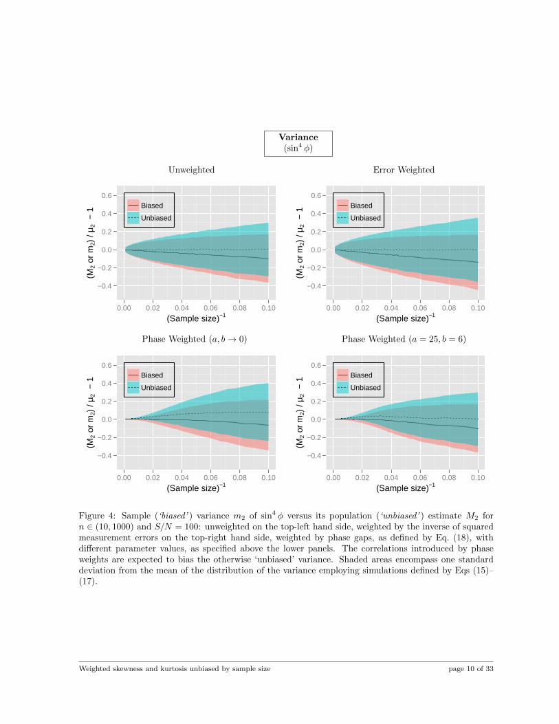
Figure 4: Sample (‘biased’ ) variance m2 of sin4 φ versus its population (‘unbiased’ ) estimate M2 forn ∈ (10, 1000) and S/N = 100: unweighted on the top-left hand side, weighted by the inverse of squaredmeasurement errors on the top-right hand side, weighted by phase gaps, as defined by Eq. (18), withdifferent parameter values, as specified above the lower panels. The correlations introduced by phaseweights are expected to bias the otherwise ‘unbiased’ variance. Shaded areas encompass one standarddeviation from the mean of the distribution of the variance employing simulations defined by Eqs (15)–(17).


Skewness(sinφ)

Unweighted

−1.0

−0.5

0.0

0.5

1.0

1.5

0.00 0.02 0.04 0.06 0.08 0.10

(Sample size)−1

(M3

or m

3) /

µ 232 −

γ1 Biased

Unbiased

Error Weighted

−1.0

−0.5

0.0

0.5

1.0

1.5

0.00 0.02 0.04 0.06 0.08 0.10

(Sample size)−1

(M3

or m

3) /

µ 232 −

γ1 Biased

Unbiased

Unweighted

−1.0

−0.5

0.0

0.5

1.0

1.5

0.00 0.02 0.04 0.06 0.08 0.10

(Sample size)−1

(G1

or g

1) −

γ1

Biased

Unbiased

Error Weighted

−1.0

−0.5

0.0

0.5

1.0

1.5

0.00 0.02 0.04 0.06 0.08 0.10

(Sample size)−1

(G1

or g

1) −

γ1

Biased

Unbiased

Figure 5: Sample (‘biased’ ) skewness m3 of sinφ versus its population (‘unbiased’ ) estimate M3 forn ∈ (10, 1000) and S/N = 100: unweighted in the upper panels and weighted by the inverse of squaredmeasurement errors in the lower panels. Shaded areas encompass one standard deviation from the meanof the distribution of the skewness employing simulations defined by Eqs (15)–(17).


Skewness(sinφ)


−1.0

−0.5

0.0

0.5

1.0

1.5

0.00 0.02 0.04 0.06 0.08 0.10

(Sample size)−1

(M3

or m

3) /

µ 232 −

γ1 Biased

Unbiased


−1.0

−0.5

0.0

0.5

1.0

1.5

0.00 0.02 0.04 0.06 0.08 0.10

(Sample size)−1

(M3

or m

3) /

µ 232 −

γ1 Biased

Unbiased


−1.0

−0.5

0.0

0.5

1.0

1.5

0.00 0.02 0.04 0.06 0.08 0.10

(Sample size)−1

(G1

or g

1) −

γ1

Biased

Unbiased


−1.0

−0.5

0.0

0.5

1.0

1.5

0.00 0.02 0.04 0.06 0.08 0.10

(Sample size)−1

(G1

or g

1) −

γ1

Biased

Unbiased

Figure 6: Sample (‘biased’ ) skewness m3 of sinφ versus its population (‘unbiased’ ) estimate M3 forn ∈ (10, 1000) and S/N = 100, weighted by phase gaps, as defined by Eq. (18), with different parametervalues, as specified above each panel. Shaded areas encompass one standard deviation from the mean ofthe distribution of the skewness employing simulations defined by Eqs (15)–(17).


Skewness(sin4 φ)

Unweighted

−1.0

−0.5

0.0

0.5

1.0

1.5

0.00 0.02 0.04 0.06 0.08 0.10

(Sample size)−1

(M3

or m

3) /

µ 232 −

γ1 Biased

Unbiased

Error Weighted

−1.0

−0.5

0.0

0.5

1.0

1.5

0.00 0.02 0.04 0.06 0.08 0.10

(Sample size)−1

(M3

or m

3) /

µ 232 −

γ1 Biased

Unbiased

Unweighted

−1.0

−0.5

0.0

0.5

1.0

1.5

0.00 0.02 0.04 0.06 0.08 0.10

(Sample size)−1

(G1

or g

1) −

γ1

Biased

Unbiased

Error Weighted

−1.0

−0.5

0.0

0.5

1.0

1.5

0.00 0.02 0.04 0.06 0.08 0.10

(Sample size)−1

(G1

or g

1) −

γ1

Biased

Unbiased

Figure 7: Sample (‘biased’ ) skewness m3 of sin4 φ versus its population (‘unbiased’ ) estimate M3 forn ∈ (10, 1000) and S/N = 100: unweighted in the upper panels and weighted by the inverse of squaredmeasurement errors in the lower panels. Estimators labeled as ‘unbiased’ but involving ratios or powers ofunbiased estimators are not expected to remain unbiased. Shaded areas encompass one standard deviationfrom the mean of the distribution of the skewness employing simulations defined by Eqs (15)–(17).


Skewness(sin4 φ)


−1.0

−0.5

0.0

0.5

1.0

1.5

0.00 0.02 0.04 0.06 0.08 0.10

(Sample size)−1

(M3

or m

3) /

µ 232 −

γ1 Biased

Unbiased


−1.0

−0.5

0.0

0.5

1.0

1.5

0.00 0.02 0.04 0.06 0.08 0.10

(Sample size)−1

(M3

or m

3) /

µ 232 −

γ1 Biased

Unbiased


−1.0

−0.5

0.0

0.5

1.0

1.5

0.00 0.02 0.04 0.06 0.08 0.10

(Sample size)−1

(G1

or g

1) −

γ1

Biased

Unbiased


−1.0

−0.5

0.0

0.5

1.0

1.5

0.00 0.02 0.04 0.06 0.08 0.10

(Sample size)−1

(G1

or g

1) −

γ1

Biased

Unbiased

Figure 8: Sample (‘biased’ ) skewness m3 of sin4 φ versus its population (‘unbiased’ ) estimate M3 forn ∈ (10, 1000) and S/N = 100, weighted by phase gaps, as defined by Eq. (18), with different parametervalues, as specified above each panel. The correlations introduced by weights are expected to bias theotherwise ‘unbiased’ skewness. Also, estimators labeled as ‘unbiased’ but involving ratios or powers ofunbiased estimators are not expected to remain unbiased. Shaded areas encompass one standard deviationfrom the mean of the distribution of the skewness employing simulations defined by Eqs (15)–(17).


Kurtosis(sinφ)

Unweighted

−2

−1

0

1

2

3

0.00 0.02 0.04 0.06 0.08 0.10

(Sample size)−1

(M4

or m

4) /

µ 22 − 3

− γ

2

Biased

Unbiased

Error Weighted

−2

−1

0

1

2

3

0.00 0.02 0.04 0.06 0.08 0.10

(Sample size)−1

(M4

or m

4) /

µ 22 − 3

− γ

2

Biased

Unbiased

Unweighted

−2

−1

0

1

2

3

0.00 0.02 0.04 0.06 0.08 0.10

(Sample size)−1

(M4

/ M22 o

r m

4 / m

22 )

− 3

− γ

2

Biased

Unbiased

Error Weighted

−2

−1

0

1

2

3

0.00 0.02 0.04 0.06 0.08 0.10

(Sample size)−1

(M4

/ M22 o

r m

4 / m

22 )

− 3

− γ

2

Biased

Unbiased

Figure 9: Sample (‘biased’ ) kurtosis m4 of sinφ versus its population (‘unbiased’ ) estimate M4 forn ∈ (10, 1000) and S/N = 100: unweighted in the upper panels and weighted by the inverse of squaredmeasurement errors in the lower panels. Estimators labeled as ‘unbiased’ but involving ratios or powers ofunbiased estimators are not expected to remain unbiased. Shaded areas encompass one standard deviationfrom the mean of the distribution of the kurtosis employing simulations defined by Eqs (15)–(17).


Kurtosis(sinφ)


−2

−1

0

1

2

3

0.00 0.02 0.04 0.06 0.08 0.10

(Sample size)−1

(M4

or m

4) /

µ 22 − 3

− γ

2

Biased

Unbiased


−2

−1

0

1

2

3

0.00 0.02 0.04 0.06 0.08 0.10

(Sample size)−1

(M4

or m

4) /

µ 22 − 3

− γ

2

Biased

Unbiased


−2

−1

0

1

2

3

0.00 0.02 0.04 0.06 0.08 0.10

(Sample size)−1

(M4

/ M22 o

r m

4 / m

22 )

− 3

− γ

2

Biased

Unbiased


−2

−1

0

1

2

3

0.00 0.02 0.04 0.06 0.08 0.10

(Sample size)−1

(M4

/ M22 o

r m

4 / m

22 )

− 3

− γ

2

Biased

Unbiased

Figure 10: Sample (‘biased’ ) kurtosis m4 of sinφ versus its population (‘unbiased’ ) estimate M4 forn ∈ (10, 1000) and S/N = 100, weighted by phase gaps, as defined by Eq. (18), with different parametervalues, as specified above each panel. The correlations introduced by weights are expected to bias theotherwise ‘unbiased’ kurtosis. Also, estimators labeled as ‘unbiased’ but involving ratios or powers ofunbiased estimators are not expected to remain unbiased. Shaded areas encompass one standard deviationfrom the mean of the distribution of the kurtosis employing simulations defined by Eqs (15)–(17).


Kurtosis(sin4 φ)

Unweighted

−2

−1

0

1

2

3

0.00 0.02 0.04 0.06 0.08 0.10

(Sample size)−1

(M4

or m

4) /

µ 22 − 3

− γ

2

Biased

Unbiased

Error Weighted

−2

−1

0

1

2

3

0.00 0.02 0.04 0.06 0.08 0.10

(Sample size)−1

(M4

or m

4) /

µ 22 − 3

− γ

2

Biased

Unbiased

Unweighted

−2

−1

0

1

2

3

0.00 0.02 0.04 0.06 0.08 0.10

(Sample size)−1

(M4

/ M22 o

r m

4 / m

22 )

− 3

− γ

2

Biased

Unbiased

Error Weighted

−2

−1

0

1

2

3

0.00 0.02 0.04 0.06 0.08 0.10

(Sample size)−1

(M4

/ M22 o

r m

4 / m

22 )

− 3

− γ

2

Biased

Unbiased

Figure 11: Sample (‘biased’ ) kurtosis m4 of sin4 φ versus its population (‘unbiased’ ) estimate M4 forn ∈ (10, 1000) and S/N = 100: unweighted in the upper panels and weighted by the inverse of squaredmeasurement errors in the lower panels. Estimators labeled as ‘unbiased’ but involving ratios or powers ofunbiased estimators are not expected to remain unbiased. Shaded areas encompass one standard deviationfrom the mean of the distribution of the kurtosis employing simulations defined by Eqs (15)–(17).


Kurtosis(sin4 φ)


−2

−1

0

1

2

3

0.00 0.02 0.04 0.06 0.08 0.10

(Sample size)−1

(M4

or m

4) /

µ 22 − 3

− γ

2

Biased

Unbiased


−2

−1

0

1

2

3

0.00 0.02 0.04 0.06 0.08 0.10

(Sample size)−1

(M4

or m

4) /

µ 22 − 3

− γ

2

Biased

Unbiased


−2

−1

0

1

2

3

0.00 0.02 0.04 0.06 0.08 0.10

(Sample size)−1

(M4

/ M22 o

r m

4 / m

22 )

− 3

− γ

2

Biased

Unbiased


−2

−1

0

1

2

3

0.00 0.02 0.04 0.06 0.08 0.10

(Sample size)−1

(M4

/ M22 o

r m

4 / m

22 )

− 3

− γ

2

Biased

Unbiased

Figure 12: Sample (‘biased’ ) kurtosis m4 of sin4 φ versus its population (‘unbiased’ ) estimate M4 forn ∈ (10, 1000) and S/N = 100, weighted by phase gaps, as defined by Eq. (18), with different parametervalues, as specified above each panel. The correlations introduced by weights are expected to bias theotherwise ‘unbiased’ kurtosis. Also, estimators labeled as ‘unbiased’ but involving ratios or powers ofunbiased estimators are not expected to remain unbiased. Shaded areas encompass one standard deviationfrom the mean of the distribution of the kurtosis employing simulations defined by Eqs (15)–(17).


k-Kurtosis(sinφ)

Unweighted

−2

0

2

4

0.00 0.02 0.04 0.06 0.08 0.10

(Sample size)−1

(K4

or k

4) /

µ 22 − γ

2

Biased

Unbiased

Error Weighted

−2

0

2

4

0.00 0.02 0.04 0.06 0.08 0.10

(Sample size)−1

(K4

or k

4) /

µ 22 − γ

2

Biased

Unbiased

Unweighted

−2

0

2

4

0.00 0.02 0.04 0.06 0.08 0.10

(Sample size)−1

(G2

or g

2) −

γ2

Biased

Unbiased

Error Weighted

−2

0

2

4

0.00 0.02 0.04 0.06 0.08 0.10

(Sample size)−1

(G2

or g

2) −

γ2

Biased

Unbiased

Figure 13: Sample (‘biased’ ) kurtosis k4 of sinφ versus its population (‘unbiased’ ) estimate K4 forn ∈ (10, 1000) and S/N = 100: unweighted in the upper panels and weighted by the inverse of squaredmeasurement errors in the lower panels. Estimators labeled as ‘unbiased’ but involving ratios or powers ofunbiased estimators are not expected to remain unbiased. Shaded areas encompass one standard deviationfrom the mean of the distribution of the kurtosis employing simulations defined by Eqs (15)–(17).


k-Kurtosis(sinφ)


−2

0

2

4

0.00 0.02 0.04 0.06 0.08 0.10

(Sample size)−1

(K4

or k

4) /

µ 22 − γ

2

Biased

Unbiased


−2

0

2

4

0.00 0.02 0.04 0.06 0.08 0.10

(Sample size)−1

(K4

or k

4) /

µ 22 − γ

2

Biased

Unbiased


−2

0

2

4

0.00 0.02 0.04 0.06 0.08 0.10

(Sample size)−1

(G2

or g

2) −

γ2

Biased

Unbiased


−2

0

2

4

0.00 0.02 0.04 0.06 0.08 0.10

(Sample size)−1

(G2

or g

2) −

γ2

Biased

Unbiased

Figure 14: Sample (‘biased’ ) kurtosis k4 of sinφ versus its population (‘unbiased’ ) estimate K4 forn ∈ (10, 1000) and S/N = 100, weighted by phase gaps, as defined by Eq. (18), with different parametervalues, as specified above each panel. The correlations introduced by weights are expected to bias theotherwise ‘unbiased’ kurtosis. Also, estimators labeled as ‘unbiased’ but involving ratios or powers ofunbiased estimators are not expected to remain unbiased. Shaded areas encompass one standard deviationfrom the mean of the distribution of the kurtosis employing simulations defined by Eqs (15)–(17).


k-Kurtosis(sin4 φ)

Unweighted

−2

0

2

4

0.00 0.02 0.04 0.06 0.08 0.10

(Sample size)−1

(K4

or k

4) /

µ 22 − γ

2

Biased

Unbiased

Error Weighted

−2

0

2

4

0.00 0.02 0.04 0.06 0.08 0.10

(Sample size)−1

(K4

or k

4) /

µ 22 − γ

2

Biased

Unbiased

Unweighted

−2

0

2

4

0.00 0.02 0.04 0.06 0.08 0.10

(Sample size)−1

(G2

or g

2) −

γ2

Biased

Unbiased

Error Weighted

−2

0

2

4

0.00 0.02 0.04 0.06 0.08 0.10

(Sample size)−1

(G2

or g

2) −

γ2

Biased

Unbiased

Figure 15: Sample (‘biased’ ) kurtosis k4 of sin4 φ versus its population (‘unbiased’ ) estimate K4 forn ∈ (10, 1000) and S/N = 100: unweighted in the upper panels and weighted by the inverse of squaredmeasurement errors in the lower panels. Estimators labeled as ‘unbiased’ but involving ratios or powers ofunbiased estimators are not expected to remain unbiased. Shaded areas encompass one standard deviationfrom the mean of the distribution of the kurtosis employing simulations defined by Eqs (15)–(17).


k-Kurtosis(sin4 φ)


−2

0

2

4

0.00 0.02 0.04 0.06 0.08 0.10

(Sample size)−1

(K4

or k

4) /

µ 22 − γ

2

Biased

Unbiased


−2

0

2

4

0.00 0.02 0.04 0.06 0.08 0.10

(Sample size)−1

(K4

or k

4) /

µ 22 − γ

2

Biased

Unbiased


−2

0

2

4

0.00 0.02 0.04 0.06 0.08 0.10

(Sample size)−1

(G2

or g

2) −

γ2

Biased

Unbiased


−2

0

2

4

0.00 0.02 0.04 0.06 0.08 0.10

(Sample size)−1

(G2

or g

2) −

γ2

Biased

Unbiased

Figure 16: Sample (‘biased’ ) kurtosis k4 of sin4 φ versus its population (‘unbiased’ ) estimate K4 forn ∈ (10, 1000) and S/N = 100, weighted by phase gaps, as defined by Eq. (18), with different parametervalues, as specified above each panel. The correlations introduced by weights are expected to bias theotherwise ‘unbiased’ kurtosis. Also, estimators labeled as ‘unbiased’ but involving ratios or powers ofunbiased estimators are not expected to remain unbiased. Shaded areas encompass one standard deviationfrom the mean of the distribution of the kurtosis employing simulations defined by Eqs (15)–(17).


A Derivation of sample-size unbiased weighted momentsThe derivations presented in this Appendix involve weighted estimators under the assumption of indepen-dent measurements and weights. Definitions and some of the relations often employed herein are listedbelow.

• Averages are weighted as θ =∑ni=1 wiθi/V1.

• Ellipses indicate the existence of terms with null expected value.

• xa and xb denote two different representatives from independent and identically distributed elementsso that, for example, E(xaxb) = E(xa)E(xb) = µ2.

•∑i is implied to sum over all (from the 1-st to the n-th) terms, unless explicitly stated otherwise.

• While E(wpi ) = wpi for the specific i-th value, for a generic weight wa it equals E(wpa) =∑i wiw

pi /V1 =

Vp+1/V1, so E(wa) = w = V2/V1, E(w2a) = V3/V1 and so on.

• V 21 =

∑i wi

∑j wj

= wa∑i wi +

∑i6=a wi

∑j wj

= w2a + wa

∑i 6=a wi + wa

∑i 6=a wi +

∑i6=a wi

∑j 6=a wj

= w2a + 2wa

∑i 6=a wi +

∑i 6=a w

2i +

∑i 6=a wi

∑j 6=i,a wj

=∑i w

2i + 2wa

∑i6=a wi +

∑i 6=a wi

∑j 6=i,a wj

= V2 + 2wa∑i 6=a wi +

∑i 6=a wi

∑j 6=i,a wj .

• V 31 =

∑i wi

∑j wj

∑k wk

= wa∑i wi

∑j wj +

∑i 6=a wi

∑j wj

∑k wk

= w2a

∑i wi + wa

∑i6=a wi

∑j wj + wa

∑i 6=a wi

∑j wj +

∑i 6=a wi

∑j 6=a wj

∑k wk

= w3a + w2

a

∑i 6=a wi + w2

a

∑i 6=a wi + wa

∑i 6=a wi

∑j 6=a wj + w2

a

∑i6=a wi +

+ wa∑i6=a wi

∑j 6=a wj + wa

∑i 6=a wi

∑j 6=a wj +

∑i 6=a wi

∑j 6=a wj

∑k 6=a wk

= w3a + 3w2

a

∑i 6=a wi + 3wa

∑i 6=a wi

∑j 6=a wj +

∑i 6=a wi

∑j 6=a wj

∑k 6=a wk

= w3a + 3w2

a

∑i 6=a wi + 3wa

∑i 6=a w

2i + 3wa

∑i 6=a wi

∑j 6=i,a wj +

∑i 6=a w

3i +

+∑i 6=a w

2i

∑j 6=i,a wj+

∑i6=a w

2i

∑j 6=i,a wj+

∑i 6=a wi

∑j 6=i,a w

2j+∑i 6=a wi

∑j 6=i,a wj

∑k 6=i,ja wk

= V3 + 3w2a

∑i 6=a wi + 3wa

∑i6=a w

2i + 3wa

∑i 6=a wi

∑j 6=i,a wj + 3

∑i 6=a w

2i

∑j 6=i,a wj +

+∑i 6=a wi

∑j 6=i,a wj

∑k 6=i,ja wk.

• V1V2 =∑i wi

∑j w

2j

= wa∑i w

2i +

∑i 6=a wi

∑j w

2j

= w3a + wa

∑i 6=a w

2i + w2

a

∑i6=a wi +

∑i 6=a wi

∑j 6=a w

2j

= w3a + wa

∑i 6=a w

2i + w2

a

∑i 6=a wi +

∑i 6=a w

3i +

∑i6=a wi

∑j 6=i,a w

2j

= V3 + wa∑i 6=a w

2i + w2

a

∑i 6=a wi +

∑i 6=a wi

∑j 6=i,a w

2j .

• V 21 − V2 =

∑i

∑j 6=i wiwj .

• V 22 − V4 =

∑i

∑j 6=i w

2iw

2j .

• wqa∑ni 6=a w

pi = VpE(wqa)− E(wp+qa ) = (VpVq+1 − Vp+q+1)/V1.

•∑i wi

∑j w

2j = w3

a + wa∑i 6=a w

2i + w2

a

∑i 6=a wi +

∑i6=a w

3i +

∑i6=a wi

∑j 6=i,a w

2j , thus∑

i 6=a wi∑j 6=i,a w

2j = V1V2 − V3 − (V 2

2 − V4)/V1 − (V1V3 − V4)/V1.

•∑i wi

∑j wj = w2

a + 2wa∑i 6=a wi +

∑i 6=a w

2i +

∑i 6=a wi

∑j 6=i,a wj , thus

wa∑i 6=a wi

∑j 6=i,a wj = V1V2 − V4/V1 − 2(V1V3 − V4)/V1 − (V 2

2 − V4)/V1.


A.1 Outline of results

The expressions of the elements pursued along the derivation of sample-size unbiased estimators (detailedin Sec. A.2) are summarized below, following the notation introduced in Sec. 2.

E[(x− µ)2

]= V2µ2/V

21 (27)

E[(x− µ)3

]= V3µ3/V

31 (28)

E[(x− µ)4

]=[V4µ4 + 3

(V 22 − V4

)µ22

]/V 4

1 (29)

E(x2a) = µ2 + µ2 (30)

E(x3a) = µ3 + 3µ2µ+ µ3 (31)

E(x4a) = µ4 + 4µ3µ+ 6µ2µ2 + µ4 (32)

E(x2) = V2µ2/V21 + µ2 (33)

E(x3) = V3µ3/V31 + 3V2µ2µ/V

21 + µ3 (34)

E(x4) = V4µ4/V41 + 3

(V 22 − V4

)µ22/V

41 + 4V3µ3µ/V

31 + 6V2µ2µ

2/V 21 + µ4 (35)

E(xax) = V2µ2/V21 + µ2 = E(x2) (36)

E(x2ax) = V2µ3/V21 +

(1 + 2V2/V

21

)µ2µ+ µ3 (37)

E(xax2) = V3µ3/V

31 + 3V2µ2µ/V

21 + µ3 = E(x3) (38)

E(x3ax) = V2µ4/V21 +

(1 + 3V2/V

21

)µ3µ+ 3

(1 + V2/V

21

)µ2µ

2 + µ4 (39)

E(xax3) = V4µ4/V

41 + 3

(V 22 − V4

)µ22/V

41 + 4V3µ3µ/V

31 + 6V2µ2µ

2/V 21 + µ4 = E(x4) (40)

E(x2ax2) = V3µ4/V

31 + 2

(V3/V

31 + V2/V

21

)µ3µ+

(1 + 5V2/V

21

)µ2µ

2 +(V2/V

21 − V3/V 3

1

)µ22 + µ4 (41)

E(m2) =(1− V2/V 2

1

)µ2 = µ2 − E

[(x− µ)2

](42)

E(m3) =(1− 3V2/V

21 + 2V3/V

31

)µ3 = µ3 − (3V1V2/V3 − 2)E

[(x− µ)3

](43)

E(m4) =(1− 4V2/V

21 + 6V3/V

31 − 3V4/V

41

)µ4 +

[6(V2/V

21 − V3/V 3

1 )− 9(V 22 − V4)/V 4

1

]µ22 (44)

=(1− 4V2/V

21 + 6V3/V

31

)µ4 + 6

(V2/V

21 − V3/V 3

1

)µ22 − 3E

[(x− µ)4

](45)

E(m22) =

(V2/V

21 − 2V3/V

31 + V4/V

41

)µ4 +

[1− 3V2/V

21 + 2V3/V

31 + 3(V 2

2 − V4)/V 41

]µ22 (46)

=(V2/V

21 − 2V3/V

31 + V4/V

41

)κ4 +

[1− 4V3/V

31 + 3V4/V

41 + 3(V 2

2 − V4)/V 41

]κ22 (47)

E(k4) =(1− 7V2/V

21 + 12V3/V

31 − 6V4/V

41

)κ4 − 6

[V2/V

21 − 4V3/V

31 + 3V4/V

41 + 3(V 2

2 − V4)/V 41

]κ22(48)

M2 =V 21

V 21 − V2

m2 = K2 (49)

M3 =V 31

V 31 − 3V1V2 + 2V3

m3 = K3 (50)

M4 =V 21 (V 4

1 − 3V 21 V2 + 2V1V3 + 3V 2

2 − 3V4)m4

(V 21 − V2)(V 4

1 − 6V 21 V2 + 8V1V3 + 3V 2

2 − 6V4)− 3V 2

1 (2V 21 V2 − 2V1V3 − 3V 2

2 + 3V4)m22

(V 21 − V2)(V 4

1 − 6V 21 V2 + 8V1V3 + 3V 2

2 − 6V4)(51)

K4 =V 21 (V 4

1 − 4V1V3 + 3V 22 )m4

(V 21 − V2)(V 4

1 − 6V 21 V2 + 8V1V3 + 3V 2

2 − 6V4)− 3V 2

1 (V 41 − 2V 2

1 V2 + 4V1V3 − 3V 22 )m2

2

(V 21 − V2)(V 4

1 − 6V 21 V2 + 8V1V3 + 3V 2

2 − 6V4)(52)


A.2 Detailed computations

E[(x− µ)2

]= E

( 1

V1

∑i

wixi − µ

)2 (53)

= E

( 1

V1

∑i

wi(xi − µ)

)2 (54)

=1

V 21

E

∑i

w2i (xi − µ)2 +

∑i

wi(xi − µ)∑j 6=i

wj(xj − µ)

(55)

=1

V 21

∑i

w2iE[(xa − µ)2

](56)

=V2V 21

µ2 (57)

E[(x− µ)3

]= E

( 1

V1

∑i

wixi − µ

)3 (58)

= E

( 1

V1

∑i

wi(xi − µ)

)3 (59)

=1

V 31

E

∑i

w3i (xi − µ)3 + 3

∑i

w2i (xi − µ)2

∑j 6=i

wj(xj − µ) + ...

(60)

=1

V 31

∑i

w3iE[(xa − µ)3

](61)

=V3V 31

µ3 (62)

E[(x− µ)4

]= E

( 1

V1

∑i

wixi − µ

)4 (63)

= E

( 1

V1

∑i

wi(xi − µ)

)4 (64)

=1

V 41

E

∑i

w4i (xi − µ)4 + 3

∑i

w2i (xi − µ)2

∑j 6=i

w2j (xj − µ)2 + ...

(65)

=1

V 41

∑i

w4iE[(xa − µ)4

]+ 3

∑i

∑j 6=i

w2iw

2jE[(xa − µ)2

]E[(xb − µ)2

]+ ...

(66)

=V4V 41

µ4 + 3V 22 − V4V 41

µ22 (67)


E(x2a) = E[(xa − µ+ µ)2] (68)

= E[(xa − µ)2] + 2µE(xa − µ) + E(µ2) (69)

= µ2 + µ2 (70)

E(x3a) = E[(xa − µ+ µ)3] (71)

= E[(xa − µ)3] + 3µE[(xa − µ)2] + 3µ2E(xa − µ) + E(µ3) (72)

= µ3 + 3µ2µ+ µ3 (73)

E(x4a) = E[(xa − µ+ µ)4] (74)

= E[(xa − µ)4] + 4µE[(xa − µ)3] + 6µ2E[(xa − µ)2] + 4µ3E(xa − µ) + E(µ4) (75)

= µ4 + 4µ3µ+ 6µ2µ2 + µ4 (76)

E(x2) = E[(x− µ+ µ)2] (77)

= E[(x− µ)2] + 2µE(x− µ) + E(µ2) (78)

= V2µ2/V21 + µ2 (79)

E(x3) = E[(x− µ+ µ)3] (80)

= E[(x− µ)3] + 3µE[(x− µ)2] + 3µ2E(x− µ) + E(µ3) (81)

= V3µ3/V31 + 3V2µ2µ/V

21 + µ3 (82)

E(x4) = E[(x− µ+ µ)4] (83)

= E[(x− µ)4] + 4µE[(x− µ)3] + 6µ2E[(x− µ)2] + 4µ3E(x− µ) + E(µ4) (84)

= V4µ4/V41 + 3(V 2

2 − V4)µ22/V

41 + 4V3µ3µ/V

31 + 6V2µ2µ

2/V 21 + µ4 (85)

E(xax) = E

(xa

1

V1

∑i

wixi

)(86)

=1

V1E

wax2a + xa∑i 6=a

wixi

(87)

=1

V1E(wax

2a) +

1

V1E(xa)

∑i 6=a

wiE(xb) (88)

=1

V1E(wa)µ2 +

1

V1waµ

2 +1

V1µ2∑i6=a

wi (89)

=1

V1

V2V1

µ2 +1

V1µ2∑i

wi (90)

=V2V 21

µ2 + µ2 = E(x2) (91)


E(x2ax) = E

(x2a

1

V1

∑i

wixi

)(92)

=1

V1E

wax3a + x2a∑i 6=a

wixi

(93)

=1

V1E(wax

3a) +

1

V1E(x2a)

∑i 6=a

wiE(xb) (94)

=1

V1E(wa)µ3 +

3

V1waµ2µ+

1

V1waµ

3 +1

V1(µ2 + µ2)µ

∑i 6=a

wi (95)

=1

V1

V2V1

µ3 +2

V1E(wa)µ2µ+

1

V1(µ2 + µ2)µ

∑i

wi (96)

=V2V 21

µ3 + 2V2V 21

µ2µ+ (µ2 + µ2)µ (97)

=V2V 21

µ3 +

(1 + 2

V2V 21

)µ2µ+ µ3 (98)

E(xax2) = E

xa( 1

V1

∑i

wixi

)2 (99)

=1

V 21

E

xa∑i

w2i x

2i + xa

∑i

wixi∑j 6=i

wjxj

(100)

=1

V 21

E

w2ax

3a + xa

∑i6=a

w2i x

2i + wax

2a

∑i 6=a

wixi + xa∑i 6=a

wixi∑j 6=i

wjxj

(101)

=1

V 21

E

w2ax

3a + xa

∑i6=a

w2i x

2i + 2wax

2a

∑i 6=a

wixi + xa∑i6=a

wixi∑j 6=i,a

wjxj

(102)

=1

V 21

E(w2a)µ3 +

3

V 21

w2aµ2µ+

1

V 21

w2aµ

3 +1

V 21

(µ2µ+ µ3)∑i 6=a

w2i+

+2

V 21

E(wa)µ2µ∑i 6=a

wi +2

V 21

waµ2µ∑i 6=a

wi +1

V 21

µ3∑i 6=a

wi∑j 6=i,a

wj (103)

=V3V 31

µ3 +1

V 21

(µ2µ+ µ3)∑i

w2i + 2

V2V 31

µ2µ∑i

wi +2

V 21

waµ3∑i6=a

wi+

1

V 21

µ3∑i 6=a

wi∑j 6=i,a

wj (104)

=V3V 31

µ3 +

(V2V 21

+ 2V2V1V 31

)µ2µ+ µ3 (105)

=V3V 31

µ3 + 3V2V 21

µ2µ+ µ3 = E(x3) (106)


E(x3ax) = E

(x3a

1

V1

∑i

wixi

)(107)

=1

V1E

wax4a + x3a∑i 6=a

wixi

(108)

=1

V1E(wax

4a) +

1

V1E(x3a)

∑i6=a

wiE(xb) (109)

=1

V1E(wa)µ4 +

3

V1E(wa)µ3µ+

1

V1waµ3µ+

3

V1E(wa)µ2µ

2 +3

V1waµ2µ

2 +1

V1waµ

4+

+1

V1

(µ3 + 3µ2µ+ µ3

)µ∑i6=a

wi (110)

=V2V 21

µ4 + 3V2V 21

µ3µ+ 3V2V 21

µ2µ2 +

1

V1

(µ3 + 3µ2µ+ µ3

)µ∑i

wi (111)

=V2V 21

µ4 +

(1 + 3

V2V 21

)µ3µ+ 3

(1 +

V2V 21

)µ2µ

2 + µ4 (112)

E(xax3) = E

xa( 1

V1

∑i

wixi

)3 (113)

=1

V 31

E

xa∑i

wixi∑j

wjxj∑k

wkxk

(114)

=1

V 31

E

xa∑i

wixi

∑j

w2jx

2j +

∑j

wjxj∑k 6=j

wkxk

(115)

=1

V 31

E

xa∑i

w3i x

3i + 3xa

∑i

wixi∑j 6=i

w2jx

2j + xa

∑i

wixi∑j 6=i

wjxj∑k 6=i,j

wkxk

(116)

=1

V 31

E

w3ax

4a + xa

∑i 6=a

w3i x

3i + 3wax

2a

∑i 6=a

w2i x

2i + 3w2

ax3a

∑i6=a

wixi + 3xa∑i 6=a

wixi∑j 6=i,a

w2jx

2j+

+3wax2a

∑i 6=a

wixi∑j 6=i,a

wjxj + xa∑i 6=a

wixi∑j 6=i,a

wjxj∑

k 6=i,j,a

wkxk

(117)

=1

V 31

E(w3a)µ4 +

4

V 31

w3aµ3µ+

6

V 31

w3aµ2µ

2 +1

V 31

w3aµ

4 +1

V 31

(µ3 + 3µ2µ+ µ3)µ∑i6=a

w3i+

+3

V 31

wa(µ2 + µ2)2∑i 6=a

w2i +

3

V 31

w2a(µ3 + 3µ2µ+ µ3)µ

∑i6=a

wi+

+3

V 31

(µ2 + µ2)µ2∑i 6=a

wi∑j 6=i,a

w2j +

3

V3wa(µ2 + µ2)µ2

∑i 6=a

wi∑j 6=i,a

wj+

+1

V 31

µ4∑i6=a

wi∑j 6=i,a

wj∑

k 6=i,j,a

wk (118)


=1

V 31

V4V1

µ4 +1

V 31

µ3µ∑i

w3i +

3

V 31

E(w2a)µ3µ

∑i

wi +6

V 31

E(w2a)µ2µ

2∑i

wi +1

V 31

µ4∑i

w3i+

+3

V 31

µ2µ2∑i 6=a

w3i +

3

V 31

wa(µ22 + µ4 + 2µ2µ

2)∑i6=a

w2i +

3

V 31

w2a(µ2µ

2 + µ4)∑i 6=a

wi+

+3

V 31

(µ2µ2 + µ4)

∑i 6=a

wi∑j 6=i,a

w2j +

3

V3wa(µ2µ

2 + µ4)∑i 6=a

wi∑j 6=i,a

wj+

+1

V 31

µ4∑i 6=a

wi∑j 6=i,a

wj∑

k 6=i,j,a

wk (119)

=V4V 41

µ4 +

(V3V 31

+ 3V3V 31

)µ3µ+ 6

V3V 31

µ2µ2 + µ4 +

3

V 31

µ2µ2∑i 6=a

w3i+

+3

V 31

waµ22

∑i 6=a

w2i +

6

V 31

waµ2µ2∑i 6=a

w2i +

3

V 31

w2aµ2µ

2∑i 6=a

wi+

+3

V 31

µ2µ2∑i 6=a

wi∑j 6=i,a

w2j +

3

V3waµ2µ

2∑i 6=a

wi∑j 6=i,a

wj (120)

=V4V 41

µ4 + 4V3V 31

µ3µ+ µ4 +3

V 31

V 22 − V4V1

µ22 +

3

V 31

(2V3 +

V1V3 − V4V1

+ 2V 22 − V4V1

+V1V3 − V4

V1+

+V1V2 − V3 −V 22 − V4V1

− V1V3 − V4V1

+ V1V2 −V4V1− 2

V1V3 − V4V1

− V 22 − V4V1

)µ2µ

2 (121)

=V4V 41

µ4 + 3V 22 − V4V 41

µ22 + 4

V3V 31

µ3µ+ 6V2V 21

µ2µ2 + µ4 = E(x4) (122)

E(x2ax2) = E

x2a(

1

V1

∑i

wixi

)2 (123)

=1

V 21

E

x2a∑i

w2i x

2i + x2a

∑i

wixi∑j 6=i

wjxj

(124)

=1

V 21

E

w2ax

4a + x2a

∑i 6=a

w2i x

2i + wax

3a

∑i 6=a

wixi + x2a∑i6=a

wixi∑j 6=i

wjxj

(125)

=1

V 21

E

w2ax

4a + x2a

∑i 6=a

w2i x

2i + 2wax

3a

∑i6=a

wixi + x2a∑i 6=a

wixi∑j 6=i,a

wjxj

(126)

=1

V 21

E(w2a)µ4 +

2

V 21

E(w2a)µ3µ+

2

V 21

w2aµ3µ+

6

V 21

w2aµ2µ

2 +1

V 21

w2aµ

4 +1

V 21

(µ2 + µ2)2∑i6=a

w2i+

+2

V 21

waµ3µ∑i 6=a

wi +6

V 21

waµ2µ2∑i6=a

wi +2

V 21

waµ4∑i 6=a

wi +1

V 21

(µ2 + µ2)µ2∑i 6=a

wi∑j 6=i,a

wj

(127)


=V3V 31

µ4 + 2V3V 31

µ3µ+2

V 21

E(wa)µ3µ∑i

wi +1

V 21

µ22

∑i 6=a

w2i +

2

V 21

µ2µ2∑i

w2i +

1

V 21

µ4∑i

w2i+

+4

V 21

E(wa)µ2µ2∑i

wi +2

V 21

waµ2µ2∑i 6=a

wi +2

V 21

waµ4∑i6=a

wi +1

V 21

µ2µ2∑i6=a

wi∑j 6=i,a

wj+

+1

V 21

µ4∑i6=a

wi∑j 6=i,a

wj (128)

=V3V 31

µ4 + 2

(V3V 31

+V2V 21

)µ3µ+

1

V 21

µ22

∑i6=a

w2i + 2

V2V 21

µ2µ2 + 4

V2V 21

µ2µ2 +

2

V 21

waµ2µ2∑i 6=a

wi+

+1

V 21

µ2µ2∑i 6=a

wi∑j 6=i,a

wj + µ4 (129)

=V3V 31

µ4 + 2

(V3V 31

+V2V 21

)µ3µ+

(1 + 5

V2V 21

)µ2µ

2 +

(V2V 21

− V3V 31

)µ22 + µ4 (130)

E(m2) = E

[1

V1

∑i

wi(xi − x)2

](131)

= E[(xa − x)2

](132)

= E(x2a − 2xax+ x2

)(133)

= E(x2a)− E(x2) (134)

= µ2 + µ2 − V2µ2/V21 − µ2 (135)

=

(1− V2

V 21

)µ2 (136)

= µ2 − E[(x− µ)2

](137)

E(m3) = E

[1

V1

∑i

wi(xi − x)3

](138)

= E[(xa − x)3

](139)

= E(x3a − 3x2ax+ 3xax

2 − x3)

(140)

= E(x3a)− 3E(x2ax) + 2E(x3) (141)

= µ3 + 3µ2µ+ µ3 − 3

[V2V 21

µ3 +

(1 + 2

V2V 21

)µ2µ+ µ3

]+ 2

(V3V 31

µ3 + 3V2V 21

µ2µ+ µ3

)(142)

=

(1− 3

V2V 21

+ 2V3V 31

)µ3 (143)

= µ3 −(

3V1V2V3− 2

)E[(x− µ)3

](144)

E(m4) = E

[1

V1

∑i

wi(xi − x)4

](145)

= E[(xa − x)4

](146)

= E(x4a)− 4E(x3ax) + 6E(x2ax2)− 4E(xax

3) + E(x4) (147)


= µ4 + 4µ3µ+ 6µ2µ2 + µ4 − 4

[V2V 21

µ4 +

(1 + 3

V2V 21

)µ3µ+ 3

(1 +

V2V 21

)µ2µ

2 + µ4

]+

+ 6

[V3V 31

µ4 + 2

(V3V 31

+V2V 21

)µ3µ+

(1 + 5

V2V 21

)µ2µ

2 +

(V2V 21

− V3V 31

)µ22 + µ4

]+

− 4

[V4V 41

µ4 + 3V 22 − V4V 41

µ22 + 4

V3V 31

µ3µ+ 6V2V 21

µ2µ2 + µ4

]+

+V4V 41

µ4 + 3V 22 − V4V 41

µ22 + 4

V3V 31

µ3µ+ 6V2V 21

µ2µ2 + µ4 (148)

=

(1− 4

V2V 21

+ 6V3V 31

− 3V4V 41

)µ4 +

[6

(V2V 21

− V3V 31

)− 9

V 22 − V4V 41

]µ22 (149)

=

(1− 4

V2V 21

+ 6V3V 31

)µ4 + 6

(V2V 21

− V3V 31

)µ22 − 3E

[(x− µ)4

](150)

E(m22) = E

( 1

V1

∑i

wi(xi − x)2

)2 (151)

= E

( 1

V1

∑i

wi(x2i − x2)

)2 (152)

=1

V 21

E

(∑i

wix2i

)2− 2

V 21

E

(x2∑i

wix2i

)+ E(x4) (153)

=1

V 21

E

∑i

w2i x

4i +

∑i

wix2i

∑j 6=i

wjx2j

− 2E(x2ax2) + E(x4) (154)

=V2V 21

(µ4 + 4µ3µ+ 6µ2µ

2 + µ4)

+V 21 − V2V 21

(µ2 + µ2

)2+

− 2

[V3V 31

µ4 + 2

(V3V 31

+V2V 21

)µ3µ+

(1 + 5

V2V 21

)µ2µ

2 +

(V2V 21

− V3V 31

)µ22 + µ4

]+

+V4V 41

µ4 + 3V 22 − V4V 41

µ22 + 4

V3V 31

µ3µ+ 6V2V 21

µ2µ2 + µ4 (155)

=

(V2V 21

− 2V3V 31

+V4V 41

)µ4 + 4

(V2V 21

− V3V 31

− V2V 21

+V3V 31

)µ3µ+

+

(6V2V 21

+ 2V 21 − V2V 21

− 2− 10V2V 21

+ 6V2V 21

)µ2µ

2 +

(V2V 21

+V 21 − V2V 21

− 2 + 1

)µ4+

+

(V 21 − V2V 21

− 2V2V 21

+ 2V3V 31

+ 3V 22 − V4V 41

)µ22 (156)

=

(V2V 21

− 2V3V 31

+V4V 41

)µ4 +

(1− 3

V2V 21

+ 2V3V 31

+ 3V 22 − V4V 41

)µ22 (157)

E(m22) =

V2V 21

(µ4 − 3µ2

2

)− 2

V3V 31

(µ4 − 3µ2

2

)+V4V 41

(µ4 − 3µ2

2

)+

+

(1− 4

V3V 31

+ 3V4V 41

+ 3V 22 − V4V 41

)µ22 (158)

=

(V2V 21

− 2V3V 31

+V4V 41

)κ4 +

(1− 4

V3V 31

+ 3V4V 41

+ 3V 22 − V4V 41

)κ22 (159)


E(k4) = E(m4)− 3E(m22) (160)

=

(1− 4

V2V 21

+ 6V3V 31

− 3V4V 41

)µ4 +

[6

(V2V 21

− V3V 31

)− 9

V 22 − V4V 41

]µ22+

− 3

[(V2V 21

− 2V3V 31

+V4V 41

)µ4 +

(1− 3

V2V 21

+ 2V3V 31

+ 3V 22 − V4V 41

)µ22

](161)

=

(1− 7

V2V 21

+ 12V3V 31

− 6V4V 41

)µ4 − 3

(1− 5

V2V 21

+ 4V3V 31

+ 6V 22 − V4V 41

)µ22 (162)

=

(1− 7

V2V 21

+ 12V3V 31

− 6V4V 41

)(µ4 − 3µ2

2

)− 6

(V2V 21

− 4V3V 31

+ 3V4V 41

+ 3V 22 − V4V 41

)µ22 (163)

=

(1− 7

V2V 21

+ 12V3V 31

− 6V4V 41

)κ4 − 6

(V2V 21

− 4V3V 31

+ 3V4V 41

+ 3V 22 − V4V 41

)κ22 (164)

E(M2) = µ2 = E(m2)

(1− V2

V 21

)−1(165)

M2 =V 21

V 21 − V2

m2 = K2 (166)

E(M3) = µ3 = E(m3)

(1− 3

V2V 21

+ 2V3V 31

)−1(167)

M3 =V 31

V 31 − 3V1V2 + 2V3

m3 = K3 (168)

E(M4) = µ4 =

{E(m4)−

[6

(V2V 21

− V3V 31

)− 9

V 22 − V4V 41

]µ22

}(1− 4

V2V 21

+ 6V3V 31

− 3V4V 41

)−1(169)

=

{E(m4)−

[6

(V2V 21

− V3V 31

)− 9

V 22 − V4V 41

] [E(m2

2)−(V2V 21

− 2V3V 31

+V4V 41

)E(M4)

]×

×(

1− 3V2V 21

+ 2V3V 31

+ 3V 22 − V4V 41

)−1}(1− 4

V2V 21

+ 6V3V 31

− 3V4V 41

)−1(170)

=

E(m4)

1− 4 V2

V 21

+ 6 V3

V 31− 3 V4

V 41

−

(6 V2

V 21− 6 V3

V 31− 9

V 22 −V4

V 41

)E(m2

2)(1− 4 V2

V 21

+ 6 V3

V 31− 3 V4

V 41

)(1− 3 V2

V 21

+ 2 V3

V 31

+ 3V 22 −V4

V 41

)×

×

1−

(6 V2

V 21− 6 V3

V 31− 9

V 22 −V4

V 41

)(V2

V 21− 2 V3

V 31

+ V4

V 41

)(

1− 4 V2

V 21

+ 6 V3

V 31− 3 V4

V 41

)(1− 3 V2

V 21

+ 2 V3

V 31

+ 3V 22 −V4

V 41

)−1 (171)

=

[V 41 E(m4)

V 41 − 4V 2

1 V2 + 6V1V3 − 3V4− V 4

1 (6V 21 V2 − 6V1V3 − 9V 2

2 + 9V4)E(m22)

(V 41 − 4V 2

1 V2 + 6V1V3 − 3V4)(V 41 − 3V 2

1 V2 + 2V1V3 + 3V 22 − 3V4)

]×

×

[1−

(6V 2

1 V2 − 6V1V3 − 9V 22 + 9V4

) (V 21 V2 − 2V1V3 + V4

)(V 4

1 − 4V 21 V2 + 6V1V3 − 3V4) (V 4

1 − 3V 21 V2 + 2V1V3 + 3V 2

2 − 3V4)

]−1(172)

M4 =V 21 (V 4

1 − 3V 21 V2 + 2V1V3 + 3V 2

2 − 3V4)m4

(V 21 − V2)(V 4

1 − 6V 21 V2 + 8V1V3 + 3V 2

2 − 6V4)− 3V 2

1 (2V 21 V2 − 2V1V3 − 3V 2

2 + 3V4)m22

(V 21 − V2)(V 4

1 − 6V 21 V2 + 8V1V3 + 3V 2

2 − 6V4)(173)


E(K4) = κ4 =

[E(k4) + 6

(V2V 21

− 4V3V 31

+ 3V4V 41

+ 3V 22 − V4V 41

)κ22

](1− 7

V2V 21

+ 12V3V 31

− 6V4V 41

)−1(174)

=

{E(k4) + 6

(V2V 21

− 4V3V 31

+ 3V4V 41

+ 3V 22 − V4V 41

)[E(m2

2)−(V2V 21

− 2V3V 31

+V4V 41

)E(K4)

]×

×(

1− 4V3V 31

+ 3V4V 41

+ 3V 22 − V4V 41

)−1}(1− 7

V2V 21

+ 12V3V 31

− 6V4V 41

)−1(175)

=

E(m4 − 3m22)

1− 7 V2

V 21

+ 12 V3

V 31− 6 V4

V 41

+6(V2

V 21− 4 V3

V 31

+ 3 V4

V 41

+ 3V 22 −V4

V 41

)E(m2

2)(1− 7 V2

V 21

+ 12 V3

V 31− 6 V4

V 41

)(1− 4 V3

V 31

+ 3 V4

V 41

+ 3V 22 −V4

V 41

)×

×

1 +6(V2

V 21− 4 V3

V 31

+ 3 V4

V 41

+ 3V 22 −V4

V 41

)(V2

V 21− 2 V3

V 31

+ V4

V 41

)(

1− 7 V2

V 21

+ 12 V3

V 31− 6 V4

V 41

)(1− 4 V3

V 31

+ 3 V4

V 41

+ 3V 22 −V4

V 41

)−1 (176)

=

[V 41 E(m4 − 3m2

2)

V 41 − 7V 2

1 V2 + 12V1V3 − 6V4+

6V 41

(V 21 V2 − 4V1V3 + 3V4 + 3V 2

2 − 3V4)E(m2

2)

(V 41 − 7V 2

1 V2 + 12V1V3 − 6V4) (V 41 − 4V1V3 + 3V4 + 3V 2

2 − 3V4)

]×

×

[1 +

6(V 21 V2 − 4V1V3 + 3V4 + 3V 2

2 − 3V4) (V 21 V2 − 2V1V3 + V4

)(V 4

1 − 7V 21 V2 + 12V1V3 − 6V4) (V 4

1 − 4V1V3 + 3V4 + 3V 22 − 3V4)

]−1(177)

K4 =V 21 (V 4

1 − 4V1V3 + 3V 22 )m4

(V 21 − V2)(V 4

1 − 6V 21 V2 + 8V1V3 + 3V 2

2 − 6V4)− 3V 2

1 (V 41 − 2V 2

1 V2 + 4V1V3 − 3V 22 )m2

2

(V 21 − V2)(V 4

1 − 6V 21 V2 + 8V1V3 + 3V 2

2 − 6V4)(178)


Weighted skewness and kurtosis unbiased by sample size - arXiv · Weighted skewness and kurtosis...

Documents

Transcript of Weighted skewness and kurtosis unbiased by sample size - arXiv · Weighted skewness and kurtosis...