Do Realized Skewness and Kurtosis Predict

the Cross-Section of Equity Returns?�

Diego Amaya Peter Christo¤ersen

HEC Montreal and UQAM Rotman, CBS and CREATES

Kris Jacobs Aurelio Vasquez

University of Houston and Tilburg University ITAM School of Business

December 26, 2011

Abstract

Yes. We use intraday data to compute weekly realized variance, skewness and kurtosis for

individual equities and assess whether this week�s realized moments predict next week�s stock

returns in the cross-section. We sort stocks each week according to their realized moments,

form decile portfolios, and analyze subsequent weekly returns. We �nd a very strong negative

relationship between realized skewness and next week�s stock returns, and a positive relationship

between realized kurtosis and next week�s stock returns. We do not �nd a strong relationship

between realized volatility and stock returns. A trading strategy that buys stocks in the lowest

realized skewness decile and sells stocks in the highest realized skewness decile generates an

average weekly return of 24 basis points with a t-statistic of 3:65. A similar strategy that buys

stocks with high realized kurtosis and sells stocks with low realized kurtosis produces a weekly

return of 14 basis points with a t-statistic of 2:12. Our results are robust across sample periods,

portfolio weightings, and �rm characteristics, and they are not captured by the Fama-French

and Carhart factors.

JEL Codes: G11, G12, G17

Keywords: Realized volatility; skewness; kurtosis; equity markets; return prediction.

�We would like to thank seminar participants at McGill University, Queen�s University, Rutgers University, RyersonUniversity, University of British Columbia, the 2010 FMA and EFMA meetings, the IFM2 Mathematical Finance Con-ference, Stanford SITE, and the Market Microstructure Conference in Paris for helpful comments. We thank IFM2,SSHRC, and Asociación Mexicana de Cultura A.C. for �nancial support. Any remaining inadequacies are ours alone.Correspondence to: Peter Christo¤ersen, Phone: 416-946-5511, Email: peter.christo¤ersen@rotman.utoronto.ca.

1

1 Introduction

We examine the relationship between higher moments computed from intraday returns and future

stock returns. Extending the well-known concept of realized volatility (Hsieh (1991), Andersen,

Bollerslev, Diebold, and Ebens (2001)), computed from intraday squared returns, we compute

realized skewness and kurtosis from intraday cubed and quartic returns. We show that the real-

ized moments have well-de�ned convergence limits under realistic assumptions and that they are

measured reliably in �nite samples.

The relationship between higher moments and stock returns has been a topic of study since

Kraus and Litzenberger (1976), who show theoretically that coskewness is a determinant of the

cross-section of stock returns. Going beyond comovements, three di¤erent types of theoretical

arguments suggest that assets� skewness may explain asset returns. Barberis and Huang (2008)

demonstrate that assets with greater skewness have lower returns under cumulative prospect the-

ory. Mitton and Vorkink (2007) obtain a similar result for expected skewness using heterogeneous

investor preference for skewness, and Brunnermeier, Gollier, and Parker (2007) also predict a neg-

ative relationship between skewness and returns using an optimal expectations framework. Theory

therefore unambiguously predicts a negative relationship between an asset�s skewness and its return.

To the best of our knowledge no such theoretical results are available for kurtosis.

Recent papers con�rm that higher moments of the underlying stock return distribution are

related to future returns. Ang, Hodrick, Xing, and Zhang (2006) �nd that stocks with higher

idiosyncratic volatility have lower subsequent returns. Boyer, Mitton, and Vorkink (2010) �nd that

stocks with higher expected idiosyncratic skewness yield lower future returns. Grouping stocks by

industry, Zhang (2006) documents a negative relation between skewness and stock returns. Kelly

(2011) studies the relationship between tail estimates and returns. Skewness measures extracted

from options yield contradictory results on the relation between option implied skewness and future

returns in the cross-section. While Xing, Zhang and Zhao (2010) and Rehman and Vilkov (2010)

document a positive relation, Conrad, Dittmar, and Ghysels (2008) �nd a negative one. As for

kurtosis, Conrad, Dittmar, and Ghysels (2008) report that risk-neutral kurtosis and stock returns

are positively related.

Our empirical strategy uses a very extensive sample of weekly data. We aggregate daily realized

moments to obtain weekly realized volatility, skewness, and kurtosis measures for over two million

�rm-week observations. We sort stocks into deciles based on the current-week realized moment and

compute the subsequent one-week return of the trading strategy that buys the portfolio of stocks

with a high realized moment (volatility, skewness or kurtosis) and sells the portfolio of stocks with

a low realized moment.

When sorting on realized volatility, the resulting portfolio return di¤erences are not statistically

signi�cant. However, when sorting by realized skewness, the long-short value-weighted portfolio

produces an average weekly return of �24 basis points with a t-statistic of �3:65. This exceeds the

2

premiums reported in Boyer, Mitton, and Vorkink (2010) and in Zhang (2006), which are �67 and�36 basis points per month, respectively. The resulting four factor Carhart risk adjusted alphafor the long-short skewness portfolio is �23 basis points per week. We �nd a positive relationbetween realized kurtosis and subsequent stock returns. For realized kurtosis, the long-short value-

weighted portfolio generates a weekly return of 14 basis points with a t-statistic of 2:12. The four

factor Carhart alpha of 11 basis points per week further supports the value of realized kurtosis as

a predictor of stock returns.

We con�rm the negative relation between realized skewness and future returns, and the positive

relation between realized kurtosis and future returns, using Fama-MacBeth regressions. We also

investigate the robustness of these �ndings to controlling for a number of well-documented deter-

minants of returns: lagged return (Jegadeesh (1990), Lehmann (1990) and Gutierrez and Kelley

(2008)), realized volatility, �rm size (Fama and French (1993)), the book-to-market ratio (Fama

and French (1993)), market beta, historical skewness, idiosyncratic volatility (Ang, Hodrick, Xing,

and Zhang (2006)), coskewness (Harvey and Siddique (2000)), maximum return (Bali, Cakici, and

Whitelaw (2009)), the number of analysts that follow the �rm (Arbel and Strebel (1982)), illiquidity

(Amihud (2002)), and the number of intraday transactions. Two-way sorts on realized skewness

and �rm characteristics also con�rm that the relationship between realized skewness and returns

is signi�cant. However, two-way sorts show that the relationship between realized kurtosis and

returns is not always signi�cant when controlling for other �rm characteristics. Finally, results for

realized skewness and realized kurtosis are robust to the January e¤ect and are signi�cant when

considering only NYSE stocks.

To verify that our measures of higher moments are not contaminated by microstructure noise,

and to make sure that we are e¤ectively measuring asymmetry and fat tails, we investigate two

additional measures of skewness and kurtosis using high frequency data. The �rst measure is

an enhanced version of the realized moment that uses the subsampling methodology suggested

by Zhang, Mykland, and Ait-Sahalia (2005) to compute realized volatility. This subsampling

methodology ensures that useful data is not ignored and provides a more robust estimator of the

realized moment. The second approach uses percentiles of the high-frequency return distribution as

alternative measures to capture skewness and kurtosis. We �nd that the negative relation between

realized skewness and future stock returns is robust to using di¤erent measures of skewness, but

the resulting long-short returns are smaller. However, the relation between realized kurtosis and

stock returns is not always positive for the alternative measures. In addition, we show that the

cross-sectional results also obtain for monthly holding periods.

We also compare the long-short returns obtained by sorting on our skewness measure with long-

short returns obtained by sorting on other available skewness measures. We �nd that sorting using

the skewness measure proposed by Zhang (2006) and the expected skewness measure proposed by

Boyer, Mitton, and Vorkink (2010) also yields negative long-short returns. However, in our sample

these returns are economically smaller than the ones we obtain using realized skewness, and they

3

are not statistically signi�cant. Sorting on historical skewness also does not produce statistically

signi�cant results. Our �ndings therefore complement and strengthen the results obtained using

alternative skewness estimates in Boyer, Mitton, and Vorkink (2010), Zhang (2006), Xing, Zhang

and Zhao (2010), but also suggest that our realized skewness measure may provide a simpler and

cleaner estimate of skewness, which therefore leads to economically and statistically stronger results.

Ang, Hodrick, Xing, and Zhang (2006) �nd that stocks with high idiosyncratic volatility earn

low returns. Motivated by their �ndings, we further explore the relationship between realized

skewness, idiosyncratic volatility and subsequent stock returns. We �nd that when idiosyncratic

volatility increases, low skewness stocks are compensated with higher returns while high skewness

stocks are compensated with lower returns. Therefore, skewness provides a partial explanation of

the idiosyncratic volatility puzzle. We also show that similar �ndings obtain when using realized

volatility instead of idiosyncratic volatility.

Finally, we verify the limiting properties of realized higher moments, based on a continuous-

time speci�cation of equity price dynamics that includes stochastic volatility and jumps. We show

how the limits of the higher realized moments are determined by the jump parameters of the

continuous-time price process. Using Monte Carlo techniques, we verify that the measurement of

the realized higher moments is robust to the presence of market microstructure noise as well as to

quote discontinuities in existence prior to decimalization. We also show that our cross-sectional

results hold up when using jump-robust measures of realized volatility to compute higher moments.

The remainder of the paper is organized as follows. Section 2 estimates the weekly realized

higher moments from intraday returns and constructs portfolios based on these moments. Section

3 computes raw and risk-adjusted returns on portfolios sorted on realized volatility, skewness and

kurtosis, and estimates Fama-MacBeth regressions including various control variables. Section 3

also investigates the interaction of volatility, skewness and returns. Section 4 contains a series of

robustness checks. Section 5 investigates the limiting properties of the realized higher moments as

well as the signi�cance of our results when using jump-robust realized volatility estimators. Section

6 concludes.

2 Constructing Moment-Based Portfolios

We �rst describe the data. We then show how the realized higher moments are computed. Finally,

we form portfolios by sorting stocks into deciles based on the weekly realized moments, and then

report on the characteristics of these portfolios.

2.1 Data

We analyze every listed stock in the Trade and Quote (TAQ) database from January 4, 1993 to

September 30, 2008. TAQ provides historical tick by tick data for all stocks listed on the New York

Stock Exchange, American Stock Exchange, Nasdaq National Market System, and SmallCap issues.

4

We record prices every �ve minutes starting at 9:30 EST and construct �ve-minute log-returns for

the period 9:30 EST to 16:00 EST for a total of 78 daily returns. We construct the �ve minute grid

by using the last recorded price within the preceding �ve-minute period. If there is no price in a

period, the return for that period is set to zero.

To ensure su¢ cient liquidity, we require that a stock has at least 80 daily transactions to

construct a daily measure of realized moments.1 The average number of intraday transactions per

day for a stock is over one thousand. The weekly realized moment estimator is the average of

the available daily estimators (Wednesday through Tuesday). Only one valid day of the realized

moment is required to have a weekly estimator. Stocks with prices below $5 are excluded from the

analysis.

We use data from three additional databases. From the Center for Research and Security Prices

(CRSP) database, we use daily returns of each �rm to calculate weekly returns (from Tuesday close

to Tuesday close), historical equity skewness, market beta, lagged return, idiosyncratic volatility,

maximum return over the previous month, and illiquidity; we use monthly returns to compute

coskewness as in Harvey and Siddique (2000);2 we use daily volume to compute illiquidity; and

we use outstanding shares and stock prices to compute market capitalization. COMPUSTAT is

used to extract the Standard and Poor�s issuer credit ratings and book values to calculate book-to-

market ratios of individual �rms. From Thomson Returns Institutional Brokers Estimate System

(I/B/E/S), we obtain the number of analysts that follow each individual �rm. These variables are

discussed in more detail in Appendix A.

2.2 Computing Realized Higher Moments

We �rst de�ne the intraday log returns for each �rm. On day t, the ith intraday return is given by

rt;i = pt�1+ iN� pt�1+ i�1

N; (1)

where pl is the natural logarithm of the price observed at time l and N is the number of return

observations in a trading day. We use �ve-minute returns so that in 6.5 trading hours we have

N = 78.

The well-known daily realized variance (Andersen and Bollerslev (1998) and Andersen, Boller-

slev, Diebold and Labys (2003)) is obtained by summing squares of intraday high-frequency returns

RDV art =XN

i=1r2t;i: (2)

As is standard, we do not estimate the mean of the high-frequency return because it is dominated

by the variance at this frequency.

1We repeated the analysis using a minimum of 100, 250 and 500 transactions instead. The results are similar.2Computing co-moments with high-frequency data is not straightforward due to synchronicity problems between

stock and index returns. We leave this problem for future research.

5

An appealing characteristic of this volatility measure compared to other estimation methods is

its model-free nature (see Andersen, Bollerslev, Diebold, and Labys (2001) and Barndor¤-Nielsen

and Shephard (2002) for details). Moreover, as we will discuss below, realized variance converges

to a well-de�ned quadratic variation limit as the sampling frequency N increases.

Given that we are interested in measuring the asymmetry of the daily return�s distribution, we

construct a measure of ex-post realized daily skewness based on intraday returns standardized by

the realized variance as follows

RDSkewt =

pNPNi=1 r

3t;i

RDV ar3=2t

: (3)

The interpretation of this measure is straightforward: negative values indicate that the stock�s

return distribution has a left tail that is fatter than the right tail, and positive values indicate the

opposite.

We are interested in extremes of the return distribution more generally, and so we also construct

a measure of realized daily kurtosis de�ned by

RDKurtt =NPNi=1 r

4t;i

RDV ar2t: (4)

The limits of the third and fourth moment when the sampling frequencyN increases will be analyzed

below as well.

Our cross-sectional asset pricing analysis below is conducted at the weekly frequency. We

therefore construct weekly realized moments from their daily counterparts as follows. If t is a

Tuesday then we compute

RV olt =

�252

5

X4

i=0RDV art�i

�1=2; (5)

RSkewt =1

5

X4

i=0RDSkewt�i; (6)

RKurtt =1

5

X4

i=0RDKurtt�i: (7)

Our cross-sectional analysis below is conducted at the weekly frequency and t will therefore denote

a week from this point on. Note that, as is standard, we have annualized the realized volatility

measure to facilitate the interpretation of results.

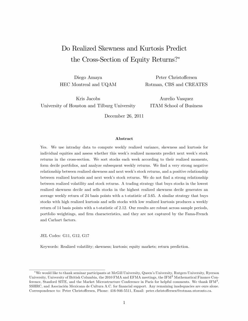
We compute the RV olt, RSkewt, and RKurtt for more than two million �rm-week observations

during our January 1993 to September 2008 sample period. Figure 1 summarizes the realized

moments. The top-left panel of Figure 1 displays a histogram of the realized volatility measure

pooled across �rms and weeks. As often found in the realized volatility literature, the unconditional

distribution of realized equity volatility appears to be roughly log-normally distributed. The top-

right panel in Figure 1 shows the time-variation in the cross-sectional percentiles using three-month

moving averages. The cross-sectional dispersion in realized equity volatility is clearly not constant

6

over time and seems to have decreased through our sample period.

The middle-left panel of Figure 1 shows the histogram of realized equity skewness. The skewness

distribution is very fat-tailed and strongly peaked around zero. The middle-right panel of Figure 1

shows the time-variation in the cross-sectional skewness percentiles. The cross-sectional dispersion

in realized equity skewness has increased through our sample.

The bottom-left panel of Figure 1 shows the histogram of realized equity kurtosis. Similar to

realized volatility, realized kurtosis appears to be approximately log-normally distributed. The vast

majority of our sample has a kurtosis above 3, strongly suggesting fat-tailed returns. The bottom-

right panel of Figure 1 shows that the cross-sectional distribution of realized equity kurtosis has

become more disperse over time, matching the result found for realized skewness.

2.3 Portfolio Sort Characteristics

Each Tuesday, we form portfolios by sorting stocks into deciles based on the weekly realized mo-

ments. Table 1 reports the time-series sample averages for the moments and di¤erent �rm character-

istics, by decile. Panel A reports the time-series averages for realized volatility, Panel B for realized

skewness, and Panel C for realized kurtosis. Column 1 represents the portfolio of stocks with the

smallest average realized moment, and column 10 is for the portfolio of stocks with the highest

realized moment. The characteristics include �rm size, book-to-market ratio, realized volatility

over the previous week, historical skewness using daily returns from the previous month, market

beta from the market model regression, lagged return, illiquidity as in Amihud (2002), coskewness

as in Harvey and Siddique (2000), idiosyncratic volatility as in Ang, Hodrick, Xing, and Zhang

(2006), the number of analysts from I/B/E/S, credit rating, stock price, the number of intraday

transactions, and the number of stocks per decile. On average there are 257 companies per decile

each week.

Table 1, Panel A displays results for the ten decile portfolios based on realized volatility. Real-

ized volatility increases from 18:8% for the �rst decile to 145:0% for the highest decile. Interestingly,

realized skewness has a negative relation with realized volatility and realized kurtosis shows an in-

creasing pattern through the volatility deciles. Furthermore, companies with high realized volatility

tend to be small, followed by fewer analysts, less coskewed with the market, and they have a lower

stock price. A positive relation exists between realized volatility and historical skewness, market

beta, lagged return, idiosyncratic volatility and maximum return. Finally, no pattern is observed

between realized volatility and book-to-market, number of intraday transactions, and credit rating.

Panel B of Table 1 shows that realized skewness equals �1:04 for the �rst decile portfolio and1:02 for the tenth decile. Firms with a high degree of asymmetry, either positive or negative, are

small, highly illiquid, followed by fewer analysts, and the number of intraday transactions for these

�rms is lower.

Panel C of Table 1 reports on the decile portfolios based on realized kurtosis. The average kur-

tosis ranges from 3:9 to 16:6 across the deciles. Firm characteristics that are positively related to

7

realized kurtosis include realized volatility, historical skewness, lagged return, idiosyncratic skew-

ness, illiquidity and maximum return. Variables that have a negative relation with realized kurtosis

include size, market beta, coskewness, number of I/B/E/S analysts, stock price, and number of in-

traday transactions.

In summary, Table 1 strongly suggests that �rm-speci�c realized volatility, skewness, and kur-

tosis all contain unique information about the cross-sectional and temporal distribution of equity

returns. We now attempt to exploit this moment-based information for predicting the cross-section

of equity returns.

3 Realized Moments and the Cross-Section of Stock Returns

In this section, we �rst analyze the relationship between the current week�s returns and the previous

week�s realized volatility, realized skewness, and realized kurtosis. Second, we use the Fama and

MacBeth (1973) methodology to conduct cross-sectional regressions and to determine the signi�-

cance of each higher realized moment individually and simultaneously, and also when controlling

for �rm-speci�c factors. Third, we investigate the interaction of returns, realized volatility and

skewness.

3.1 Sorting Stock Returns on Realized Volatility

Every Tuesday, stocks are ranked into deciles according to their realized volatility. Then, using

returns over the following week, we construct value- and equal-weighted portfolios. Table 2, Panel

A reports the time series average of weekly returns for decile portfolios based on the level of realized

volatility.

The value-weighted returns show a decreasing pattern, from 20 basis points for decile 1 to 8

basis points for decile 10. On the other hand, equal-weighted returns increase from 22 basis points

to 27 basis points. Thus, the returns of the long-short portfolio, namely one that buys stocks

in decile 10 and sells stocks in decile 1, are negative for value-weighted portfolios and positive

for equal-weighted ones. The negative relation between individual volatility and stock returns

for value-weighted portfolios is consistent with Ang, Hodrick, Xing, and Zhang (2006). However,

neither the value-weighted nor the equal-weighted long-short portfolios are statistically signi�cant,

and this is the case for raw returns as well as for alphas from the Carhart four factor model. The

four factor model employs the three Fama and French (1993) factors (excess market-return, size

and book-to-market factors) and the Carhart (1997) momentum factor.

We conclude that realized volatility and future stock returns are not robustly related when

using our measure of realized volatility.

8

3.2 Sorting Stock Returns on Realized Skewness

Table 2, Panel B reports the time-series average of weekly returns for decile portfolios grouped by

realized skewness.

The value-weighted and equal-weighted returns both show a monotonically decreasing pattern

between realized skewness and the average stock returns over the subsequent week. The return

for the portfolio of stocks with the lowest level of skewness is 40 basis points for value-weighted

portfolios and 55 basis points for equal-weighted portfolios, while the returns for stocks with the

highest level of realized skewness is 17 basis points for value-weighted and 12 for equal-weighted

portfolios. The weekly return di¤erence between portfolio 10 and 1 is �24 basis points for value-weighted returns and �43 for equal-weighted returns. Both di¤erences are statistically signi�cantat the one percent level. This result is consistent with recent theories stating that stocks with lower

skewness command a risk premium. For prominent examples, see Barberis and Huang (2008),

Brunnermeier, Gollier, and Parker (2007), and Mitton and Vorkink (2007). The equal-weighted

return di¤erence is larger than the value-weighted return di¤erence, suggesting that the relationship

between skewness and subsequent returns is larger for small �rms.

We also assess the empirical relationship between realized skewness and stock returns by ad-

justing for standard measures of risk. Panel B of Table 2 presents, for each decile, alphas relative to

the Carhart four factor model. Note that alphas are large and statistically signi�cant for value- and

equal-weighted portfolios across deciles. In addition, the di¤erence between the alphas of the tenth

and �rst deciles is �23 and �46 basis points for value- and equal-weighted portfolios, respectively.Note also that the magnitude of the alphas is very similar to that of raw returns, which shows that

standard measures of risk do not account for the return provided by the realized skewness exposure.

The sign of the cross-sectional relationship between skewness and subsequent stock returns is

consistent with the �ndings of other studies that use di¤erent measures of skewness, but the magni-

tude is larger. Boyer, Mitton, and Vorkink (2010) use a model that incorporates �rm characteristics

in order to measure the expected skewness over a given horizon. They report that a strategy that

buys stocks with the highest one-month expected skewness and sells stocks with the smallest one-

month expected skewness generates an average return of �67 basis points per month. Zhang (2006)measures expected skewness for a stock by allocating it into a peer group (e.g. industry) and uses

recent returns from this group to compute its skewness measure. In this case the long-short strategy

produces risk-adjusted returns of �36 basis points per month.Our long-short skewness returns are also large when compared with the standard four factor

returns. In our sample the weekly return on the market factor is 12 basis points per week, the size

factor return is 2 basis points, the value factor return is 10 basis points and momentum yields 20

basis points per week on average.

In conclusion, we �nd strong evidence that realized skewness predicts the cross section of stock

returns. Realized skewness is an important determinant of the cross-sectional variation in subse-

quent one-week returns, and its e¤ect is not captured by standard measures of risk.

9

3.3 Sorting Stock Returns on Realized Kurtosis

Panel C of Table 2 documents the average next-week stock returns for decile portfolios based on

realized kurtosis. Value-weighted and equal-weighted portfolio returns both increase with the level

of realized kurtosis. For value weighted portfolios, decile 1 has an average weekly return of 17

basis points, compared to 31 basis points for decile 10. Thus, the long-short portfolio generates a

return of 14 basis points with a t-statistic of 2:12. A similar result is found for the equal-weighted

portfolio, where the long-short realized kurtosis premium equals 16 basis points with a t-statistic

of 2:98.

The results for the Carhart four-factor alpha are of the same magnitude as those of the raw

returns. The value-weighted alpha for the long-short portfolio is 11 basis points and the equal-

weighted alpha is 13 basis points. The equal-weighted alpha is signi�cant at the 1% level, the

value-weighted alpha at the 5% level.

Comparing Panels A, B, and C of Table 2, we conclude that, while the results for kurtosis

are fairly strong, realized skewness appears to be the most reliable moment-based predictor of

subsequent one-week equity returns in the cross section.

3.4 Fama-MacBeth Regressions

To further assess the relationship between future returns and realized volatility, realized skewness,

and realized kurtosis, we carry out various cross-sectional regressions using the method proposed in

Fama and MacBeth (1973). Each week t, we compute the realized moments for �rm i and estimate

the following cross-sectional regression on the week t+ 1 returns

ri;t+1 = 0;t + 1;tRV oli;t + 2;tRSkewi;t + 3;tRKurti;t + �0tZi;t + "i;t+1; (8)

where ri;t+1 is the weekly return (in bps) of the ith stock for week t+ 1, and where Zi;t represent

a vector of characteristics and controls for the ith �rm observed at the end of week t: The char-

acteristics and controls included are the week t return (in bps), �rm size, book-to-market, market

beta, historical skewness, idiosyncratic volatility, coskewness, maximum monthly return (in bps),

number of analysts, illiquidity, and number of intraday transactions.

Table 3 reports the time-series average of the and � coe¢ cients for six cross-sectional regres-

sions. The �rst column presents the results of the regression of the stock return on lagged realized

volatility. The coe¢ cient associated with realized volatility is 3:5 with a Newey-West t-statistic

of 0:26. This con�rms that there does not seem to be a signi�cant relationship between realized

volatility and stock returns. The second and third columns con�rm the relation between the stock

return and lagged realized skewness and realized kurtosis respectively. In column 2, the coe¢ cient

associated with realized skewness is �22:4 with a Newey-West t-statistic of �7:90. Similarly, incolumn 3, the coe¢ cient on realized kurtosis is 1:3 with a t-statistic of 3:49. In the fourth column,

we report regression results using all higher moments simultaneously. The coe¢ cients on lagged

10

realized skewness and realized kurtosis remain statistically signi�cant, and are again negative and

positive respectively. The third and fourth realized moments appear to explain di¤erent aspects of

stock returns.

In the �fth column, we include lagged returns in the regression, given the strong evidence of the

return reversal e¤ect in short run returns (Jegadeesh (1990), Gutierrez and Kelley (2008)). Even

though the coe¢ cient of realized skewness decreases to �3:9, it remains signi�cant and negative.The coe¢ cient of realized kurtosis increases to 1:6 with a Newey-West t-statistic of 3:83. The

coe¢ cient on lagged return is negative and statistically signi�cant, as expected.

In the last column, we add all control variables to ensure that realized skewness and realized

kurtosis are not a manifestation of previously documented relationships between �rm characteristics

and stock returns. We �nd that the coe¢ cients of realized skewness and realized kurtosis are still

signi�cant, with Newey-West t-statistics of �2:73 and 2:15, and preserve their signs with coe¢ cientsof �4:7 and 0:7, respectively. The negative sign on the coe¢ cient related to size and the positivesign of the coe¢ cient related to book-to-market con�rm existing results in the literature. We

include control variables related to the illiquidity and visibility of individual stocks. This includes

the number of intraday transactions, the measure of illiquidity proposed in Amihud (2002), and

the number of analysts following a stock (see Arbel and Strebel (1982)). We also control for

the previously documented relationships between stock returns and �rm characteristics, such as

idiosyncratic volatility (Ang, Hodrick, Xing, and Zhang (2006)), the maximum daily return over

the previous month (Bali, Cakici, and Whitelaw (2009)), and the stock�s coskewness, as measured

by the variability of the stock�s return with respect to changes in the level of volatility following

Harvey and Siddique (2000). Finally, we control for the market beta computed with a regression

using daily returns on the market over the previous 12 months.

The results in the last column of Table 3 show that the economic and statistical signi�cance

of realized skewness and realized kurtosis for the cross-section of weekly returns is robust to the

inclusion of various control variables. Variables such as realized volatility, idiosyncratic volatility,

and coskewness do not play a signi�cant role in the cross-section of returns at a weekly level, while

variables such as lagged return, maximum daily return, and size are relevant.

3.5 Realized Skewness and Realized Volatility

We now further examine the interaction between the e¤ects of realized skewness and realized volatil-

ity on returns. We construct portfolios using a double sort on realized skewness and realized volatil-

ity and then examine subsequent stock returns. First, we form �ve quintile portfolios with di¤erent

levels of realized skewness. Within each of these portfolios, we form �ve portfolios that have dif-

ferent levels of realized volatility.3 Panel B of Table 4 reports the equal-weighted returns for the

25 portfolios as well as the di¤erence between the high realized volatility quintiles and low realized

volatility quintiles. We observe that in low skewness portfolios, higher realized volatility translates

3Sorting on realized volatility �rst, and subsequently on realized skewness, does not change the results.

11

into higher returns. The portfolio that buys quintile 5 (stocks with high realized volatility and low

realized skewness) and sells quintile 1 (stocks with low realized volatility and low realized skewness)

has a weekly return of 47 basis points with a t-statistic of 3:31. Hence, in the case of low skewness

stocks, investors are compensated with higher returns when holding high volatility stocks. How-

ever, for stocks with high skewness, we �nd that portfolios containing stocks with low volatility

have higher subsequent returns than portfolios containing stocks with high volatility. In this case,

the long-short portfolio return premium is �28 basis points with a t-statistic of �2:22. Overall, theportfolio with the lowest return is the one with stocks that have high skewness and high volatility.

Panel A of Table 4 demonstrates that similar results obtain for value-weighted portfolios, but in

this case the results are not statistically signi�cant.

Panel A of Figure 2 shows the value- and equal-weighted returns for the 25 portfolios double

sorted on realized skewness and realized volatility. For equal-weighted returns in the right panel,

realized skewness increases from �0:772 to +0:762 and realized volatility increases from 20% to

about 120% for the 25 portfolios. Portfolios with low realized volatility of 20% have very similar

returns for all �ve levels of realized skewness: between 20 and 30 basis points for equal-weighted

portfolios. However, as realized volatility increases, the return of low and high realized skewness

portfolios strongly diverges. Portfolios with high realized volatility of 120% report the highest and

the lowest return of all 25 portfolios. Stocks with the lowest realized skewness earn the highest

average equal-weighted return of 77 basis points; and stocks with the highest realized skewness earn

the lowest average return of �9 basis points. Hence, it is important to account for skewness whenanalyzing the return/volatility relationship. Highly volatile stocks may earn low returns, which

seems counterintuitive, but the reason is that their skewness is high.4

3.6 Realized Skewness and Idiosyncratic Volatility

Building on our �ndings regarding volatility and skewness, we now investigate whether realized

skewness can explain the idiosyncratic volatility puzzle uncovered by Ang, Hodrick, Xing, and

Zhang (2006). They �nd that stocks with high idiosyncratic volatility earn lower returns than

stocks with low idiosyncratic volatility, contradicting the implications of mean-variance models.

Table 5 replicates the idiosyncratic volatility puzzle in Ang, Hodrick, Xing, and Zhang (2006) for

our sample. For value-weighted portfolios (Panel A of Table 5), we �nd a weekly premium of

�0:24% with a t-statistic of �1:73 for the period 1993-2008. This result is comparable to that ofAng, Hodrick, Xing, and Zhang (2006) who �nd a monthly premium of �1:06% with a t-statistic of�3:10 for the period 1963-2000. Interestingly, Panel B of Table 5 indicates that the puzzle does notobtain for equal-weighted portfolios, where we do not observe signi�cant di¤erences across quintiles.

To study the interaction between realized skewness and idiosyncratic volatility on stock returns

we employ double sorting. We �rst sort stocks by realized skewness and form quintile portfolios.

4This �nding is supported by Golec and Tamarkin (1998), who show that gamblers at horse races accept bets withlow returns and high volatility only because they enjoy the high positive skewness o¤ered by these bets.

12

Quintile 1 has stocks with the lowest level of realized skewness and quintile 5 has stocks with the

highest level of realized skewness. Then, within each quintile portfolio, we sort stocks by idiosyn-

cratic volatility.5 Table 6 reports the results for value-weighted and equal-weighted portfolios. The

equal-weighted portfolio results (Panel B) are very similar to those for realized volatility reported in

Panel B of Table 4. In particular, we observe that the premium of the high idiosyncratic volatility

portfolio (quintile 5) minus the low idiosyncratic volatility portfolio (quintile 1) decreases as the

level of skewness increases. The premium for low realized skewness is 35 basis points and decreases

to �43 basis points for high realized skewness. The highest returns are observed for the portfolioswith low skewness and the lowest return of �20 basis points is for the portfolio with high idiosyn-cratic volatility and high skewness. Panel B of Figure 2 shows the returns of the 25 equal-weighted

portfolios for di¤erent levels of idiosyncratic volatility. Just as with realized volatility in Panel

A of Figure 2, high idiosyncratic volatility is compensated with high returns only if skewness is

low. Investors are willing to accept low returns and high idiosyncratic volatility in exchange for

high positive skewness. Panel A of Table 6 and Panel B of Figure 2 indicate that value-weighted

portfolios display a similar but less signi�cant pattern.

Investors trade high idiosyncratic volatility and low returns for high skewness, because they

prefer skewness. Preference for skewness seems to partly explain the idiosyncratic volatility puzzle.

4 Robustness Analysis

In this section, we further explore the relation between realized moments and stock returns. First,

we investigate if the relation between current-week realized moments and next-week returns is

present in di¤erent subsamples. Second, we check if our �ndings are robust to alternative measures

of skewness and kurtosis. Third, we investigate if the relation between moments and subsequent

returns exists regardless of �rm characteristics. Fourth, we use monthly rather than weekly holding

periods for returns.

4.1 Subsamples

Panel A of Table 7 reports value- and equal-weighted returns of portfolios sorted on realized skew-

ness across di¤erent subsamples. Keim (1983) documents calendar-related anomalies for the month

of January, in which stocks have higher returns than in the rest of the year. Panel A of Table

7 presents the average weekly returns for the month of January and for the rest of the year for

both value- and equal-weighted portfolios. As expected, returns for the month of January are

consistently higher than returns for the rest of the year.

The di¤erence between the returns of portfolios with high-skewness stocks and portfolios with

low-skewness stocks is negative and signi�cant for both January and non-January periods. This is

5An unconditional two-way sort on realized volatility and realized skewness produces similar results than theconditional two-way sort.

13

the case for value-weighted as well as equal-weighted portfolios.

We previously documented that stocks with high and low levels of skewness tend to be small.

Hence, we examine if the e¤ect of skewness is exclusively driven by small NASDAQ stocks. By

only including stocks from the New York Stock Exchange (NYSE), row 3 of Table 7 shows that the

e¤ect of realized skewness is present among NYSE stocks. Hence, small NASDAQ stocks are not

driving our results.

In Table 7, Panel B, we analyze the value-weighted and equal-weighted returns of portfolios

sorted on realized kurtosis for di¤erent subsamples. The long-short portfolio returns are positive

for all subsamples. As expected, in January the long-short portfolio earns higher returns compared

to the rest of the year. We also con�rm that the e¤ect of realized kurtosis is not driven by small

NASDAQ stocks. For value-weighted portfolios the realized kurtosis premium is positive, but often

not statistically signi�cant.

4.2 Alternative Measures of Skewness and Kurtosis

The analysis of alternative measures of skewness and kurtosis serves two purposes. On the one

hand we want to investigate if our �ndings depend on the implementation of the realized skewness

and kurtosis measures. On the other hand the literature already contains analyses of skewness

measures that are constructed in a radically di¤erent way. A natural question is if the long-short

returns constructed using these alternative skewness measures are similar to the long-short returns

we document in Table 2.

First, we investigate the robustness with respect to the implementation of realized skewness

by analyzing two alternative estimators. The �rst estimator, SubRSkew; uses the subsampling

methodology suggested by Zhang, Mykland, and Ait-Sahalia (2005), which provides measures ro-

bust to microstructure noise. This method consists of constructing subsamples that are spaced

every minute. Instead of one realized measure based on a single �ve-minute return grid, we end up

with �ve estimators of realized skewness using subsamples of 5-minute returns for the period 9:30

EST to 16:00 EST. Subsamples start every minute (at 9:00, 9:01, 9:02, 9:03 and 9:04), but we use

5-minute returns. Subsequently, the realized skewness estimator is computed as the average of the

�ve (overlapping) estimators obtained from the subsamples.6

The second alternative estimator of intraday skewness depends solely on quartiles from the

intraday return distribution. As proposed in Bowley (1920), a measure of skewness that is based

on quartiles can be de�ned as

SK2t = (Q3 +Q1 � 2Q2)=(Q3 �Q2); (9)

where Qi is the ith quartile of the �ve-minute return distribution F , that is Q1 = F�1 (0:25),

6Neuberger (2011) has recently suggested another interesting alternative measure of realized skewness which wehave not pursued here.

14

Q2 = F�1 (0:5), and Q3 = F�1 (0:75).

The literature contains some radically di¤erent approaches to measuring (expected) skewness.

Zhang (2006) measures the skewness for a given �rm by the cross-sectional skewness of the �rms

in that industry. Boyer, Mitton, and Vorkink (2010) construct a measure of expected idiosyncratic

skewness that controls for �rm characteristics. These two measures are discussed in more detail in

Appendix A.7

Table 8 includes our results for RSkew from Table 2, for the SK2 measure based on quartiles in

(9), and for the estimator SubRSkew which is based on the subsampling methodology suggested by

Zhang, Mykland, and Ait-Sahalia (2005). Furthermore, we include simple historical skewness com-

puted using daily returns over di¤erent horizons. The problem with computing historical skewness

from daily returns is well-known: one needs a su¢ ciently long window to capture outliers that iden-

tify skewness, but longer windows may lead to arti�cial smoothness in the resulting skewness series.

We report results for one-year, two-year, and �ve-year historical skewness. We also investigated

one-month and six-month skewness, but we did not obtain signi�cant estimates using these win-

dows. We also include the industry skewness implemented by Zhang (2006), IndSkewRes, and the

expected idiosyncratic skewness as constructed in Boyer, Mitton, and Vorkink (2010), ExpSkew.

Table 8 reports on the long-short returns. For value-weighted returns, we obtain statistically

signi�cant negative long-short returns for the alternative measures SubRSkew and SK2. However,

the long-short return is smaller than that of the RSkew measure. Out of the three measures of

historical skewness, only the 60-month yields a negative long-short return, but it is not statistically

signi�cant. The same holds for the measure in Zhang (2006), IndSkewRes, and for ExpSkew,

the measure from Boyer, Mitton, and Vorkink (2010). We performed an elaborate robustness

analysis with respect to the implementation of these measures, and we obtained similar results.

Conclusions for the equal-weighted returns largely con�rm the value-weighted results. The most

important di¤erence is that the long-short return for the RSkew measure is much larger, and as a

result the di¤erence with the long-short returns for the SK2 and SubRSkew measures is larger.

In summary, we conclude that all measures of realized skewness yield statistically signi�cant

negative long-short returns, consistent with theory. The estimate of a long-short value-weighted

return of �24 basis points obtained using RSkew is larger than the estimates obtained using alter-native measures of realized skewness, and alternative skewness measures mostly yield estimates that

are not statistically signi�cant. The equal-weighted estimate for RSkew is much larger, suggesting

that the relationship is stronger for small �rms. Interestingly, point estimates obtained using the

SK2 and SubRSkew measures are not very di¤erent from the estimate obtained using ExpSkew

7Using the methodology in Bakshi, Kapadia, and Madan (2003), Conrad, Dittmar, and Ghysels (2008) extracthigher risk neutral moments from equity options and �nd that subsequent stock returns are negatively related to riskneutral volatility, negatively related to risk neutral skewness, and positively related to risk neutral kurtosis. Using thesame methodology, Rehman and Vilkov (2010) and Xing, Zhang and Zhao (2010) �nd a positive relation between riskneutral skewness and future stock returns. It is di¢ cult to compare these measures with physical skewness becauserisk premia are large. Moreover, these risk neutral measures can only be reliably estimated for a relatively limitednumber of stocks.

15

in the equal-weighted case.

For kurtosis, we also implemented two alternative estimators. The �rst kurtosis estimator uses

the subsampling methodology suggested by Zhang, Mykland, and Ait-Sahalia (2005). The second

alternative measure for intraday kurtosis uses the octiles of the intraday return distribution as

proposed by Moors (1988). In particular, the centered kurtosis measure is de�ned as

KR2t = ((E7 � E5) + (E3 � E1))=(E6 � E2)� 1:23;

where Ei is the ith octile of the �ve-minute return distribution F , that is Ei = F�1 (i=8).

We do not report on the two alternative measures of realized kurtosis, because they produced

mixed results for the long-short portfolio returns. While the KR2 measure con�rms the positive

long-short returns, the subsampling measure produces small negative returns. None of the long-

short returns is statistically signi�cant. This con�rms that the results for realized kurtosis are less

robust than those for realized skewness.

4.3 Realized Moments and other Firm Characteristics

This section further analyzes the interaction between realized moments and other �rm characteris-

tics. Consider size as an example. As pointed out by Fama and French (2008), to ensure the validity

of an anomaly, small (microcaps), medium, and large �rms ought to all exhibit the anomaly. We use

a double sorting methodology to analyze the realized skewness premium and the realized kurtosis

premium for �ve di¤erent size portfolios. We �rst sort stocks into quintiles by size and then, within

each quintile, we sort stocks again by realized skewness (or realized kurtosis) into quintiles. Then

we compute the value- and equal-weighted return for each portfolio and the di¤erence between the

highest and lowest realized skewness (or kurtosis) quintiles. This di¤erence represents a realized

skewness (or kurtosis) premium conditional on size. This double sorting methodology analyzes the

value- and equal-weighted return of the long-short portfolio, quintile 5 minus quintile 1, for each

size quintile. With this methodology, we can assess if the realized moment premium is economically

signi�cant for all size levels. We also provide a similar analysis for the following �rm characteristics:

lagged return, market beta, BE/ME, realized volatility, historical skewness, illiquidity, number of

intraday transactions, maximum return over the previous month, number of I/B/E/S analysts,

idiosyncratic volatility and coskewness. We perform all analyses for realized skewness and realized

kurtosis. Realized volatility is not included, because its relation with future stock returns is not

statistically signi�cant.

Panel A of Table 9 reports the value- and equal-weighted results for skewness. In row 1, we

double sort stock returns on realized skewness across di¤erent levels of �rm size and, for each

�rm size quintile, we compute the return of the portfolio that buys the highest realized skewness

stocks (within a given size quintile) and sells the lowest realized skewness stocks (within that same

size quintile). For value-weighted returns, the realized skewness premium of �75 basis points for

16

quintile 1 can be earned by buying small stocks (microcaps) with high realized skewness and selling

small stocks with low realized skewness. For big �rms in quintile 5, the corresponding premium

is �26 basis points. All �ve size groups exhibit the realized skewness anomaly, but the premiumis larger for small stocks. This �nding explains why the e¤ect of realized skewness is weaker

for value-weighted portfolios when compared to equal-weighted portfolios, as evident in Table 2.

The stronger negative e¤ect of skewness for small �rms is also consistent with Chan, Chen, and

Hsieh (1985), who show that there are risk di¤erences between small and large �rms. The realized

skewness premium and t-statistics are of similar magnitude for equal-weighted returns.

Panel A of Table 9 reports realized skewness premia for value- and equal-weighted portfolios

conditional on the various �rm characteristics. For value-weighted returns the realized skewness

premia are negative and statistically signi�cant in most cases. Only two quintiles yield positive

returns when double sorting by lagged return and one quintile is not signi�cant when double sorting

by book-to-market. For equal weighted portfolios, the realized skewness premia are negative and

statistically signi�cant for all �rm characteristics. The relationship between realized skewness and

subsequent returns is robust to all �rm characteristics and is not a proxy for any of them.

In the previous section, Fama-MacBeth regressions showed that lagged returns have explanatory

power for next-week returns. The third row in Panel A of Table 9 shows that realized skewness is

negatively associated with next week value-weighted returns for quintiles 1 to 3 of lagged return, and

that the e¤ect is stronger for past losers (stocks with the smallest lagged return). For equal-weighted

returns, the realized skewness premia are negative for any level of lagged return. Furthermore, as

the market beta increases, the long-short skewness premium becomes more negative. This pattern

is also observed for idiosyncratic volatility or realized volatility, con�rming the results in Tables 4

and 6.

Panel B of Table 9 reports value- and equal-weighted results from a double sort on realized

kurtosis and �rm characteristics. The results are more robust for equal- than for value-weighted

portfolios and are not as strong as those for realized skewness since not all realized kurtosis premia

are statistically signi�cant. Overall, it is clear from Table 9 that realized skewness is a stronger

predictor of future stock returns than realized kurtosis.

4.4 Monthly Returns

Thus far our empirics have been based on weekly returns and weekly realized moments. In this

section we keep the weekly frequency when computing realized moments but we increase the return

holding period from one week to one month.

Table 10 contains the results for overlapping monthly returns. As for the weekly returns in Table

2, we report the value-weighted and equal-weighted returns of decile portfolios formed from realized

moments, and the return di¤erence between portfolio 10 (highest realized moment) and portfolio 1

(lowest realized moment). Each panel reports on both value-weighted and equal-weighted portfolios

and include t-statistics computed from robust standard errors. Alpha is again computed using the

17

Carhart four factor model.

Panel A reports the results for realized volatility. The insigni�cant relationship between volatil-

ity and weekly returns found in Panel A of Table 2 is evident for monthly returns in Table 10 as

well.

Panel B in Table 10 reports the relationship between realized skewness and subsequent monthly

returns. The strong negative relationship between realized skewness and returns in Table 2 is

con�rmed when using monthly returns. This relationship is signi�cant for raw returns as well as

alphas, and for value-weighted and equal-weighted portfolios.

Finally, Panel C in Table 10 reports the cross-sectional relationship between weekly realized

kurtosis and monthly returns. The positive relationship found for weekly returns in Table 2 is also

evident for monthly returns in Table 10. The relationship appears to be stronger for equal-weighted

returns than for value-weighted returns when using a one-month holding period. This was also the

case for weekly returns in Table 2.

5 Properties of Realized Moments

The limiting properties of realized variance have been studied in detail in the econometrics litera-

ture, however, much less is known about realized skewness and kurtosis. In this section we therefore

investigate the realized moments when assuming that the underlying continuous time price process

follows a jump-di¤usion with stochastic volatility. First, we derive closed-form solutions for the

limits of the realized moments. Second, we allow for market microstructure noise and discontinu-

ities in quoted prices, and provide Monte Carlo evidence on the realized higher moments. Third,

we assess the signi�cance of our cross-sectional return results when using jump-robust measures of

realized volatility.

5.1 The Equity Price Process

To illustrate the properties of the realized moments de�ned in (2), (3), and (4), we assume that

the log-price pt of a security evolves according to the stochastic di¤erential equation

dpt =��� 1

2Vt � �J��dt+

pVtdW

(1)t + JdNt; (10)

dVt = � (� � Vt) dt+ �pVtdW

(2)t ; (11)

where � is the drift parameter, � is the mean reversion speed to the long-term volatility mean �,

and � is the di¤usion coe¢ cient of the volatility process Vt. W(1)t and W (2)

t denote two standard

Brownian motions with correlation �, and Nt is an independent Poisson process with arrival rate

�. The jump size J is distributed N��J ; �

2J

�.

18

5.2 The Limits of the Realized Moments

Suppose that in the time interval [0; T ], for example a day, N + 1 observations are available on p,

and the distance between these observations is � = T=N , that is, the observation times are ti = i� ,

for i = 0; : : : ; N . Then we de�ne the realized moments by

RM (j) =

NXi=0

�pti+1 � pti

�j (12)

for j = 1, 2, 3, 4. The limits of these realized moments are given in the following proposition:

Proposition 1 The realized moments de�ned in (12) for j = 1, 2, 3, and 4 converge in mean

square to the integrated moments

IM (1) =

��� �

2

�T + (� � V0)

�1� e��T

��

; (13)

IM(2) =�� + �

��2J + �

2J

��T � (� � V0)

�1� e��T

��

; (14)

IM(3) = ���3J + 3�J�

2J

�T; (15)

IM(4) = ���4J + 6�

2J�

2J + 3�

4J

�T: (16)

Proof. See Appendix B.

This result is quite revealing. Note that while the limit for j = 2 contains both jump and

di¤usion parameters, the limits for j = 3 and j = 4 depend exclusively on jump parameters. This

means that realized skewness and realized kurtosis, as de�ned in equations (3) and (4), complement

the information captured by realized volatility. IM(3), which is the limit of the numerator in

RDSkew, is the only realized moment that accounts for the jump direction, since its sign depends

on that of the average jump size, �J . IM(4), which is the limit of the numerator in RDKurt,

captures the magnitude of the jump.

5.3 Allowing for Market Microstructure Noise

So far, we have studied the realized moments in the idealized case where observed prices correspond

to their theoretical counterparts. In practice, microstructure noise is present in high frequency

prices. To simulate market microstructure noise, we de�ne the observed log price p�t as

p�t = pt + ut; (17)

where ut is i.i.d. Gaussian noise with mean zero and variance �2u. Hence, the observed log price p�t

is a noisy observation of the non-observable true price pt:

Several studies use Monte Carlo simulations to investigate the properties of realized variance

estimators when allowing for market microstructure noise, see for instance Andersen, Bollerslev,

19

and Meddahi (2011), Gonçalves and Meddahi (2009), and Ait-Sahalia and Yu (2009). Following

their work, we conduct the following Monte Carlo study. We simulate 100; 000 paths of the log

price process pt using the Euler scheme at a time interval � = 1 second. The parameters for the

continuous part of the process are set to � = 0:05, � = 5, � = 0:04, � = 0:5, V0 = 0:09, and

� = �0:5. The parameters for the jump component are set at � = 100, �J = 0:01 and �J = 0:05.The microstructure noise, ut, is modeled with a normal distribution of mean zero and standard

deviation of 0:05%. These parameter values are similar to those employed by Ait-Sahalia and Yu

(2009).

To assess the impact of the microstructure noise at di¤erent sampling frequencies, we use

signature plots as proposed in Andersen, Bollerslev, Diebold, and Labys (2000). The signature

plots provide the sample mean of a daily realized moment based on returns sampled at di¤erent

intraday frequencies: We take as an observation period T = 1 day, that is T = 1=252, and we

assume a day has 6:5 trading hours.

Panel A of Figure 3 shows the signature plots of RM(j) (as de�ned in (12)) for j = 2, 3, and

4. This �gure includes 99% con�dence bands around the Monte Carlo estimates. For the second

moments in the �rst row of panels the con�dence intervals are very tight around the Monte Carlo

estimate making them barely noticeable in the plot. For the third and fourth moments (the second

and third row of panels), the 99% con�dence intervals contain the Monte Carlo estimate as well as

the theoretical limit.

The signature plot for the second moment RM(2) depicts the well-known e¤ect that microstruc-

ture noise has on realized volatility: as the sampling frequency increases (moving from right to left

in the �gure), the variance of the noise dominates that of the price process; but for lower frequen-

cies, this e¤ect attenuates. In contrast, the microstructure noise does not a¤ect the signature plots

of RM(3) and RM(4) in the same way. There is a small and insigni�cant bias in RM(3) and

RM(4) relative to IM(3) and IM(4) but the bias does not increase with the intraday frequency.

5.4 Allowing for Quoted Price Discontinuity

Chakravarty, Wood, and Van Ness (2004) document that bid-ask spreads declined signi�cantly fol-

lowing the decimalization of NYSE-listed companies in 2001. This indicates that pre-decimalization

prices exhibit an additional bid-ask spread generated by fractional minimum increments. To gauge

the e¤ect of this discontinuity on the realized moment measures, we conduct a Monte Carlo study

similar to the one above, with the exception that observed prices are now measured in sixteenths

of a dollar. To isolate the e¤ect of fractional minimum increments, we assume here that observed

prices are not a¤ected by microstructure noise.

Panel B of Figure 3 shows the signature plots for the realized moments. The plots reveal that

realized volatility is the only moment a¤ected by fractional changes in observed prices. As the

frequency increases, the discontinuity of observed prices creates noise that is picked up by the

volatility measure. However, the noise does not a¤ect the third and fourth moments as shown by

20

the 99% con�dence intervals, which contain the Monte Carlo estimate as well as the theoretical

limit.

In summary, we �nd that the third and fourth moments used in this paper have well-de�ned

limits. Moreover, when estimated with an adequate sampling frequency, realized moments are not

contaminated by simple market microstructure noise or discontinuous quotes.

5.5 Alternative Realized Volatility Estimators

For the a¢ ne jump-di¤usion model that we assumed in (10)-(11) the limit of the sum of intraday

squared returns in (14) can be written as the sum of jump variation and integrated variance

IM(2) = JV + IV

where

JV � ���2J + �

2J

�T

IV � �T + (V0 � �)�1� e��T

��

The RDV art estimator in (2) that we have used in the empirics so far will capture both jumps

and di¤usive volatility in the limit. This does not invalidate it as an ex-post measure for the total

daily quadratic variation, but it does suggest the use of more re�ned procedures for separately

estimating IV and JV .

Several volatility estimators that are robust to jumps have been developed in the literature.

They are designed to only capture IV and not JV in the limit. The so-called bipower variation

estimator of Barndor¤-Nielsen and Shephard (2004) is de�ned by

BPVt =�

2

N

N � 1

N�1Xi=1

jrt;i+1j jrt;ij

which converges in the limit to integrated variance, IVt, when N approaches in�nity, even in the

presence of jumps.

Motivated by the presence of large jumps that may bias upward the bipower variation measure

in realistic settings when N is �nite, Andersen, Dobrev and Schaumburg (2010) have recently

developed two alternative jump-robust estimators, de�ned by

MinRVt =�

� � 2

�N

N � 1

�N�1Xi=1

min fjrt;ij ; jrt;i+1jg2 ; and

MedRVt =�

6� 4p3 + �

�N

N � 2

�N�1Xi=2

median fjrt;i�1j ; jrt;ij ; jrt;i+1jg2

21

These estimators will also both converge to IVt when N goes to in�nity and in the presence of large

jumps they typically have better �nite sample properties than BPVt.

To assess the robustness of our cross-sectional return results, we report in Table 11 the equal-

weighted and value-weighted weekly returns of the di¤erence between portfolio 10 (highest realized

moment) and portfolio 1 (lowest realized moment) when using the three alternative realized volatil-

ity estimators, BPVt, MinRVt and MedRVt. To facilitate comparisons, the �rst column of Table

11 uses the standard RV olt from (5) and thus reproduces the last column of Table 2. Each panel

in Table 11 reports the equal-weighted and the value-weighted long-short returns. Alpha is again

computed using the Carhart four factor model.

Panel A in Table 11 reports the long-short results for the three alternative realized volatility

estimators. We �nd that the insigni�cant relationship between return and volatility remains when

alternative estimators of realized volatility are used.

Panel B in Table 11 shows the long-short results for realized skewness when scaling by the three

alternative realized volatility estimators. We see that the strong negative relationship between

realized skewness and return found in Table 2 is robust to changing the denominator in

RDSkewt =

pNPNi=1 r

3t;i

RDV ar3=2t

: (18)

to be any of the three jump-robust volatility estimators de�ned in this section.

Panel C in Table 11 presents the realized kurtosis results when scaling by the three alternative

realized volatility estimators. Panel C shows that the positive relationship between return and

realized kurtosis is also robust to changing the denominator in RDKurtt to be any of the jump-

robust volatility estimators.

We conclude that the strong negative relationship between skewness and subsequent returns in

the cross-section, as well as the positive relationship between kurtosis and subsequent returns, are

not artefacts of the particular measure of realized volatility that we used above. The results hold

up when we use estimators of realized volatility that are jump-robust.

6 Conclusions

We document the cross-sectional relationship between realized higher moments of individual stocks

and future stock returns. We �rst introduce model-free estimates of higher moments based on the

methodology used by Hsieh (1991) and Andersen, Bollerslev, Diebold, and Ebens (2001) to estimate

realized volatility. We use �ve-minute returns to obtain a daily measure of realized volatility,

realized skewness, and realized kurtosis, and subsequently aggregate this measure up to the weekly

frequency. We �nd that realized skewness and realized kurtosis predict next week�s stock returns

in the cross-section, but realized volatility does not.

Realized skewness is negatively related to future stock returns. Value-weighted portfolios with

22

low skewness outperform portfolios with high skewness by 24 basis points per week. Realized

kurtosis is positively related to future stock returns. A portfolio that buys stocks with high realized

kurtosis and sells stocks with low realized kurtosis generates an average weekly return of 14 basis

points.

Fama-MacBeth regressions and double sorting con�rm that realized skewness is not a proxy

for �rm characteristics such as lagged return, size, book-to-market, realized volatility, market beta,

historical skewness, idiosyncratic volatility, coskewness, maximum return over the previous month,

analysts coverage, illiquidity or number of intraday transactions. The forecasting ability of realized

kurtosis is also found to be robust to these �rm characteristics when employing Fama-MacBeth re-

gressions. However, when double sorting using �rm characteristics, the predictive power of realized

kurtosis weakens.

We analyze the relationship between realized skewness and realized volatility in more detail.

When double sorting on realized skewness and volatility, we �nd that stocks with negative skewness

are compensated with high future returns. However, as skewness increases and becomes positive,

the positive relation between volatility and returns turns into a negative relation. We conclude that

investors may accept low returns and high volatility because they are attracted to high positive

skewness.

We perform a similar analysis for realized skewness and idiosyncratic volatility. We �nd that

portfolios with high idiosyncratic volatility compensate investors with higher returns only for low

levels of skewness. For high levels of skewness, high idiosyncratic volatility leads to lower returns.

This �nding may help explain the idiosyncratic volatility puzzle in Ang, Hodrick, Xing, and Zhang

(2006), who document that stocks with high idiosyncratic volatility earn low returns.

23

References

Ait-Sahalia, Y., and J. Yu, 2009, High Frequency Market Microstructure Noise Estimates and

Liquidity Measures, Annals of Applied Statistics 3, 422-457.

Amihud, Y., 2002, Illiquidity and Stock Returns: Cross-Section and Time-Series E¤ects, Journal

of Financial Markets 5, 31-56.

Andersen, T.G., and T. Bollerslev, 1998, Answering the Skeptics: Yes, Standard Volatility Models

Do Provide Accurate Forecasts, International Economic Review 39, 885-905.

Andersen, T.G., T. Bollerslev, F. Diebold, and H. Ebens, 2001, The Distribution of Realized Stock

Return Volatility, Journal of Financial Economics 61, 43-76.

Andersen, T.G., T. Bollerslev, F.X. Diebold, and P. Labys, 2000, Great Realizations, Risk, 105-108.

Andersen, T.G., T. Bollerslev, F.X. Diebold, and P. Labys, 2001, The Distribution of Realized

Exchange Rate Volatility, Journal of the American Statistical Association 96, 42-55.

Andersen, T.G., Bollerslev, T., Diebold, F.X. and P. Labys, 2003, Modeling and Forecasting Real-

ized Volatility, Econometrica, 71, 529-626.

Andersen, T.G., T. Bollerslev, and N. Meddahi, 2011, Realized Volatility Forecasting and Market

Microstructure Noise, Journal of Econometrics 160, 220-234.

Andersen, T.G., Dobrev, D. and E. Schaumburg, 2010, Jump-Robust Volatility Estimation Using

Nearest Neighbor Truncation, Federal Reserve Bank of New York Sta¤ Report No. 465.

Ang, A., R.J. Hodrick, Y. Xing, and X. Zhang, 2006, The Cross-Section of Volatility and Expected

Returns, Journal of Finance 61, 259-299.

Arditti, F., 1967, Risk and the Required Return on Equity, Journal of Finance 22, 19�36.

Arbel, A., and P. Strebel, 1982, The Neglected and Small Firm E¤ects, Financial Review 17,

201-218.

Bakshi, G., N. Kapadia, and D. Madan, 2003, Stock Return Characteristics, Skew Laws, and the

Di¤erential Pricing of Individual Equity Options, Review of Financial Studies 16, 101-143.

Bali, T., N. Cakici, and R. Whitelaw, 2009, Maxing Out: Stocks as Lotteries and the Cross-Section

of Expected Returns, Journal of Financial Economics 99, 427-446.

Barndor¤-Nielsen, O.E., and N. Shephard, 2002, Econometric Analysis of Realised Volatility and

its Use in Estimating Stochastic Volatility Models, Journal of the Royal Statistical Society 64,

253-280.

24

Barndor¤-Nielsen, O.E., and N. Shephard, 2004, Power and Bipower Variation with Stochastic

Volatility and Jumps, Journal of Financial Econometrics 2, 1-37.

Barberis, N., and M. Huang, 2008, Stocks as Lotteries: The Implications of Probability Weighting

for Security Prices, American Economic Review 98, 2066�2100.

Bowley, A.L., 1920, Elements of Statistics, Scribner�s, New York.

Boyer, B., T. Mitton, and K. Vorkink, 2010, Expected Idiosyncratic Skewness, Review of Financial

Studies 23, 169-202.

Brunnermeier, M., C. Gollier , and J. Parker, 2007, Optimal Beliefs, Asset Prices and the Reference

for Skewed Returns, American Economic Review 97, 159-165.

Campbell, R. H., and A. Siddique, 2000, Conditional Skewness in Asset Pricing Tests, Journal of

Finance 55, 1263�1295.

Carhart, M., 1997, On Persistence in Mutual Fund Performance, Journal of Finance 52, 57-82.

Chan, K.C., N. Chen, and D.A. Hsieh, 1985, An Exploratory Investigation of the Firm Size E¤ect,

Journal of Financial Economics 14, 451-471.

Chakravarty, S., R. A. Wood, and R. A. Van Ness, 2004, Decimals And Liquidity: A Study Of The

NYSE, Journal of Financial Research 27, 75�94.

Conrad, J., R.F. Dittmar, and E. Ghysels, 2008, Ex Ante Skewness and Expected Stock Returns,

University of North Carolina, Working Paper.

Dittmar, R.F., 2002, Nonlinear Pricing Kernels, Kurtosis Preference, and Evidence from the Cross

Section of Equity, Journal of Finance 57, 369-403.

Du¢ e, D., J. Pan, and K. Singleton, 2000, Transform Analysis and Asset Pricing for A¢ ne Jump-

Di¤usions, Econometrica 68, 1343�1376.

Fama, E., and K. French, 1993, Common Risk Factors in the Returns on Stocks and Bonds, Journal

of Financial Economics 33, 3-56.

Fama, E., and K. French, 2008, Dissecting Anomalies, Journal of Finance 63, 1653-1678.

Fama, E., and M. J. MacBeth, 1973, Risk, Return, and Equilibrium: Empirical Tests, Journal of

Political Economy 81, 607-636.

Golec, J., and M. Tamarkin, 1998, Bettors Love Skewness, Not Risk, at the Horse Track, Journal

of Political Economy 106, 205-225.

Gonçalves, S., and N. Meddahi, 2009, Bootstrapping Realized Volatility, Econometrica 77, 283-306.

25

Gutierrez Jr, R., and E. Kelley, 2008, The Long-Lasting Momentum in Weekly Returns, Journal

of Finance 63, 415-447.

Harvey, C., and A. Siddique, 2000, Conditional Skewness in Asset Pricing Tests, Journal of Finance

55, 1263-1295.

Hsieh, D., 1991, Chaos and Nonlinear Dynamics: Application to Financial Markets, Journal of

Finance, 46, 1839-1877.

Jegadeesh, N., 1990, Evidence of Predictable Behavior of Security Returns, Journal of Finance 45,

881-898.

Keim, D.B., 1983, Size-Related Anomalies and Stock Return Seasonality, Journal of Financial

Economics 12, 13-32.

Kelly, B., 2011, Tail Risk and Asset Prices, Chicago Booth Research Paper No. 11-17.

Kraus, A., and R. Litzenberger, 1976, Skewness Preference and the Valuation of Risk Assets,

Journal of Finance 31, 1085-1100.

Lehmann, B.N., 1990, Fads, Martingales, and Market E¢ ciency, Quarterly Journal of Economics

105, 1-28.

Mitton, T., and K. Vorkink, 2007, Equilibrium Underdiversi�cation and the Preference for Skew-

ness, Review of Financial Studies 20, 1255-1288.

Moors, J.J.A., 1988, A Quantile Alternative for Kurtosis, The Statistician 37, 25�32.

Neuberger, A., 2011, Realized Skewness, Working Paper, Warwick Business School.

Rehman, Z., and G. Vilkov, 2010, Risk-Neutral Skewness: Return Predictability and Its Sources,

Working Paper, BlackRock and Goethe University.

Scott, R., and P. Horvath, 1980, On the Direction of Preference for Higher Order Moments, Journal

of Finance 35, 915-919.

Xing, Y., X. Zhang, and R. Zhao, 2010, What Does Individual Option Volatility Smirks Tell Us

about Future Equity Returns?, Journal of Financial and Quantitative Analysis 45, 641-662.

Zhang, L., P. Mykland, and Y. Ait-Sahalia, 2005, A Tale of Two Time Scales: Determining Inte-

grated Volatility with Noisy High-Frequency Data, Journal of the American Statistical Associ-

ation 100, 1394-1411.

Zhang, Y., 2006, Individual Skewness and the Cross-Section of Average Stock Returns, Working

Paper.

26

Appendix A: Data

� Following Fama and French (1993), size (in billions of dollars) is computed each June as thestock price times the number of outstanding shares. The market equity value is held constant

for a year.

� Following Fama and French (1993), book-to-market is computed as the ratio of book commonequity over market capitalization (size). Book common equity is de�ned using COMPUS-

TAT�s book value of stockholders�equity plus balance-sheet deferred taxes and investment

tax credit minus the book value of preferred stock. The ratio is then computed as the book

common equity at the end of the �scal year over size at the end of December.

� Historical skewness for stock i on day t is de�ned as

HSkewi;t =1

N

NPs=0

�ri;t�s � �i

�i

�3; (19)

where N is the number of trading days, ri;t�s is the daily log-return of stock i on day t� s,

�i is the mean over the last month for stock i and �i is the standard deviation of stock i for

that month. We use 20 trading days to estimate historical skewness.

� Market beta is computed at the end of each month using a regression of daily returns overthe past 12 months.

� Following Ang, Hodrick, Xing, and Zhang (2006), idiosyncratic volatility is de�ned as

idvoli;t =qvar("i;t); (20)

where "i;t is the error term of the three-factor Fama and French (1993) regression. The

regression is estimated with daily returns over the previous 20 trading days.

� Following Harvey and Siddique (2000), coskewness is de�ned as

CoSkewi;t =E�"i;t"

2m;t

�rEh"2i;t

iE�"2m;t

� ; (21)

where "i;t is obtained from "i;t = ri;t � �i � �irm;t, where ri;t is the monthly return of stock

i on month t, rm;t is the market monthly return on month t. This regression is estimated at

the end of each month using monthly returns for the past 24 months.8

8Harvey and Siddique (2000) use data for the past 60 months to estimate coskewness. This approach considerablyreduces our sample of �rms. We therefore estimate coskewness using only 24 months, which is also done in Harveyand Siddique (2000).

27

� Following Zhang (2006), industry skewness is the cross-sectional intra-group return skewnesscomputed from daily raw returns over one month. Industry skewness is de�ned as

IndSkewi;t =

Pi(Ri � IndMeani;t)

IndStd3i;t

where Ri are the daily raw returns of all stocks on industry i over one month, and IndMeani;t

and IndStdi;t are the mean and standard deviation of the daily raw returns of all stocks on

industry i over one month. There are 49 industries according to the classi�cation system

available on Kenneth French�s website.

The industry skewness residual, IndSkewResi;t, is the residual of the regression of IndSkewi;ton IndMeani;t.

� Following Boyer, Mitton, and Vorkink (2010), expected idiosyncratic skewness is computedin three steps. In the �rst step, the residual "i;d of the Fama and French (1993) three factor

model is computed on day d for �rm i over the number of days in the set N(t). The regression

coe¢ cients that de�ne the residual are estimated with daily returns over a �ve year period.

Then, idiosyncratic volatility and idiosyncratic skewness are de�ned as

ivi;t =

�1

N(t)

X"2i;d

�1=2;

isi;t =1

N(t)

P"3i;d

iv3i;t:

In the second stage, we estimate the following cross-sectional regressions at the end of each

month t

isi;t = �0;t + �1;tisi;t�60 + �2;tivi;t�60 + �3;tmomi;t�60 + �4;tturni;t�60

+�5;tsmalli;t�60 + �6;tmediumi;t�60 + �7;tNASDAQi;t�60

+�industry;tIndustryDummyi;t�60:

In this equation, momi;t�60 is the momentum de�ned as the cumulative return for �rm i over

months t�72 and t�61, turni;t�60 is the average daily turnover of the �rm over month t�60,smalli;t�60 and mediumi;t�60 are dummy variables for the �rms in �rst and second terciles

according to their market capitalization, NASDAQi;t�60 is a dummy variable for the �rms

trading on NASDAQ, and IndustryDummyi;t�60 is an industry dummy based on the two

digit SIC code classi�cation system available on Kenneth French�s website. In the �nal stage,

we use the regression coe¢ cients of the previous regression to estimate expected idiosyncratic

28

skewness for each �rm,

ExpSkewi;t = �0;t + �1;tisi;t + �2;tivi;t + �3;tmomi;t + �4;tturni;t

+�5;tsmalli;t + �6;tmediumi;t + �7;tNASDAQi;t

+�industry;tIndustryDummyi;t:

� Maximum return is de�ned as the maximum daily return over the previous month.

� Following Amihud (2002), stock illiquidity on day t is measured as the average of the ratio ofthe absolute value of the return over the dollar value of the trading volume over the previous

year

illiquidityi;t =1

N

NPs=0

�jri;t�sj

jvolumei;t�s � pricei;t�sj

�; (22)

where N is the number of trading days, ri;t�s is the daily log-return of stock i on day t� s,

volumei;t�s is the daily volume of stock i on day t� s and pricei;t�s is the price of stock i onday t� s. We use 252 trading days to estimate illiquidity.

� The credit rating is retrieved from COMPUSTAT and is then assigned a numerical value as

follows: AAA=1, AA+=2, AA=3, AA-=4, A+=5, A=6, A-=7, BBB+=8, BBB=9, BBB-

=10, BB+=11, BB=12, BB-=13, B+=14, B=15, B-=16, CCC+=17, CCC=18, CCC-=19,

CC=20, C=21 and D=22. When no rating is available, the default credit rating value is 8.

Appendix B: Limits of Realized Moments

The process for the log-price pt in equation (10) belongs to the class of models commonly known

as a¢ ne jump di¤usion models. The a¢ ne structure of this process yields closed-form solutions for

the moment generating function, MGF. In this appendix, we �nd an explicit representation of the

MGF of pti � pti�1 , which is then used to prove the limits of the realized measures.

Corollary 1 The MGF of pt is given by

t(u) = E [ exp (~u � [pT ; VT ]|)j Ft]

= e�(u;T�t)+upt+�2(u;T�t)V0 ;

where

� (u; t) = (�� ��J)ut+��

�2

�( + b) t+ 2 log

�1� + b

2

�1� e� t

���+ �t (� (u)� 1) ;

�2 (u; t) = �a�1� e� t

�2 � ( + b) (1� e� t) ;

29

where a = u � u2, b = ��u � �, =pb2 + a�2, and ~u = [u; 0]|. Ft denotes the information set

generated by the process [pt; Vt]| :

Proof. Using the transform analysis in Du¢ e, Pan, and Singleton (2000), we have that

E [ exp (~u � [pT ; VT ]|)j Ft] = exp (A (~u; t) + B (~u; t) � [pt; Vt]|) ;

where B (t) = [�1 (t) ; �2 (t)]| and ~u = [u; 0]|. Solving the system of ODEs

_B (t) =

"0 0

�12 ��

#"�1 (t)

�2 (t)

#+1

2

"0

1

#"�1 (t)

�2 (t)

#| "0 0

�12 ��

#"�1 (t)

�2 (t)

#;

_A (t) =

"�� ��J��

#�"�1 (t)

�2 (t)

#+ � (� (u)� 1) ;

with A (T ) = u and B (T ) = [u; 0]| concludes the proof.Armed with the MGF of pt, we can now derive the MGF for pti+1 � pti :

Corollary 2 The MGF of pti+1 � pti is given by

't (u; �) = E [ exp (u (pt+� � pt))j F0]

= exp (� (u; �)) exp

� (u; �) e��t

1� � (u; �) �22� (1� e��t)

!�1� � (u; �) �

2

2�

�1� e��t

��� 2���2

Proof. From the de�nition of the MGF and using the law of iterated expectations, we have:

E [ exp (u (pt+� � pt))j F0] = E [E [ exp (u (pt+� � pt))j Ft]j F0]

= E [ exp (� (u; �) + � (u; �)Vt)j F0]

= exp (� (u; �))E [ exp (� (u; �)Vt)j F0]

= exp (� (u; �)) exp (�A (�� (u; �) ; t)�B (�� (u; �) ; t)V0) ;

where

A (&; t) =&e��t

1 + & �2

2� (1� e��t); B (&; t) =

2��

�2log

�1 + &

�2

2�

�1� e��t

��;

are the coe¢ cients of the a¢ ne representation of the MGF for Vt.

To prove Proposition 1, we need to �nd the expected value of the limits of the realized moments

de�ned in (12). The following proposition establishes these limits.

Corollary 3 The limit

limN!1

E

"NXi=1

�pti � pti�1

�j# (23)

converges to (13), (14),(15) and (16) for j = 1, 2, 3 and 4, respectively.

30

Proof. We start by rewriting equation (23) as

limN!1

E

"NXi=1

�pti � pti�1

�j#= lim

N!1

NXi=1

Eh�pti � pti�1

�ji= lim

N!1

NXi=1

@j't@uj

(u; �)

����u=0

:

The Taylor series expansion of @j't@uj

(u; �)���u=0

around � = 0 yields

@'t@u

(u; �)

����u=0

=

��� �

2+1

2e��t (� � V0)

�� +O

��2�; (24)

@2't@u2

(u; �)

����u=0

=

�� + �

��2J + �

2J

�� 12e��t (� � V0)

�� +O

��2�; (25)

@3't@u3

(u; �)

����u=0

= ���3J + 3�J�

2J

�� +O

��2�; (26)

@4't@u4

(u; �)

����u=0

= ���4J + 6�

2J�

2J + 3�

4J

�� +O

��2�; (27)

where O (�)2 denotes all terms of order 2 and above. As N tends to in�nity, � converges to zero,

so that the only remaining terms in equations (24), (25), (26), and (27) are those of order 1. The

limit of the sum of these terms coincides with the de�nition of the Riemann-Stieltjes integral, so

that integrating these terms with respect to t over the sampling interval [0; T ] gives (13), (14), (15),

and (16) :

Corollary 4 The limit of the variance of the realized moments is

limN!1

NXi=1

V arh�pti � pti�1

�ji= 0;

for j = 1, 2, 3 and 4.

Proof. Follows by arguments similar to those made to prove (23).

The results in this appendix ensure mean-squared or L2 convergence of the realized moments.

31

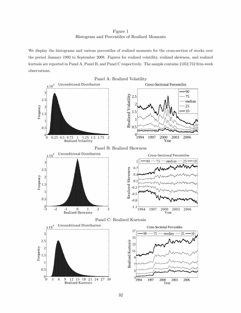
Figure 1Histogram and Percentiles of Realized Moments

We display the histograms and various percentiles of realized moments for the cross-section of stocks over

the period January 1993 to September 2008. Figures for realized volatility, realized skewness, and realized

kurtosis are reported in Panel A, Panel B, and Panel C respectively. The sample contains 2,052,752 �rm-week

observations.

Panel A: Realized Volatility

0 0.25 0.5 0.75 1 1.25 1.5 1.75 20

0.5

1

1.5

2

2.5

3

x 104

Realized Volatility

Freq

uenc

y

Unconditional Distribution

1994 1997 2000 2003 20060

0.5

1

1.5

2

2.5

Year

Rea

lized

 Vol

atili

ty

Cross­Sectional Percentiles

9075median2510

Panel B: Realized Skewness

­3 ­2 ­1 0 1 2 30

0.5

1

1.5

2

2.5

3

x 104

Realized Skewness

Freq

uenc

y

Unconditional Distribution

1994 1997 2000 2003 2006­1.1

­0.8

­0.5

­0.2

0.1

0.4

0.7

1

Year

Rea

lized

 Ske

wne

ss

Cross­Sectional P ercentiles

90 75 median 25 10

Panel C: Realized Kurtosis

0 3 6 9 12 15 18 21 24 27 300

0.5

1

1.5

2

2.5

3

x 104

Realized Kurtosis

Freq

uenc

y

Unconditional Distribution

1994 1997 2000 2003 20063

5

7

9

11

13

15

17

Year

Real

ized

 Kur

tosi

s

Cross­Sectional Percentiles

90 75 median 25 10

32

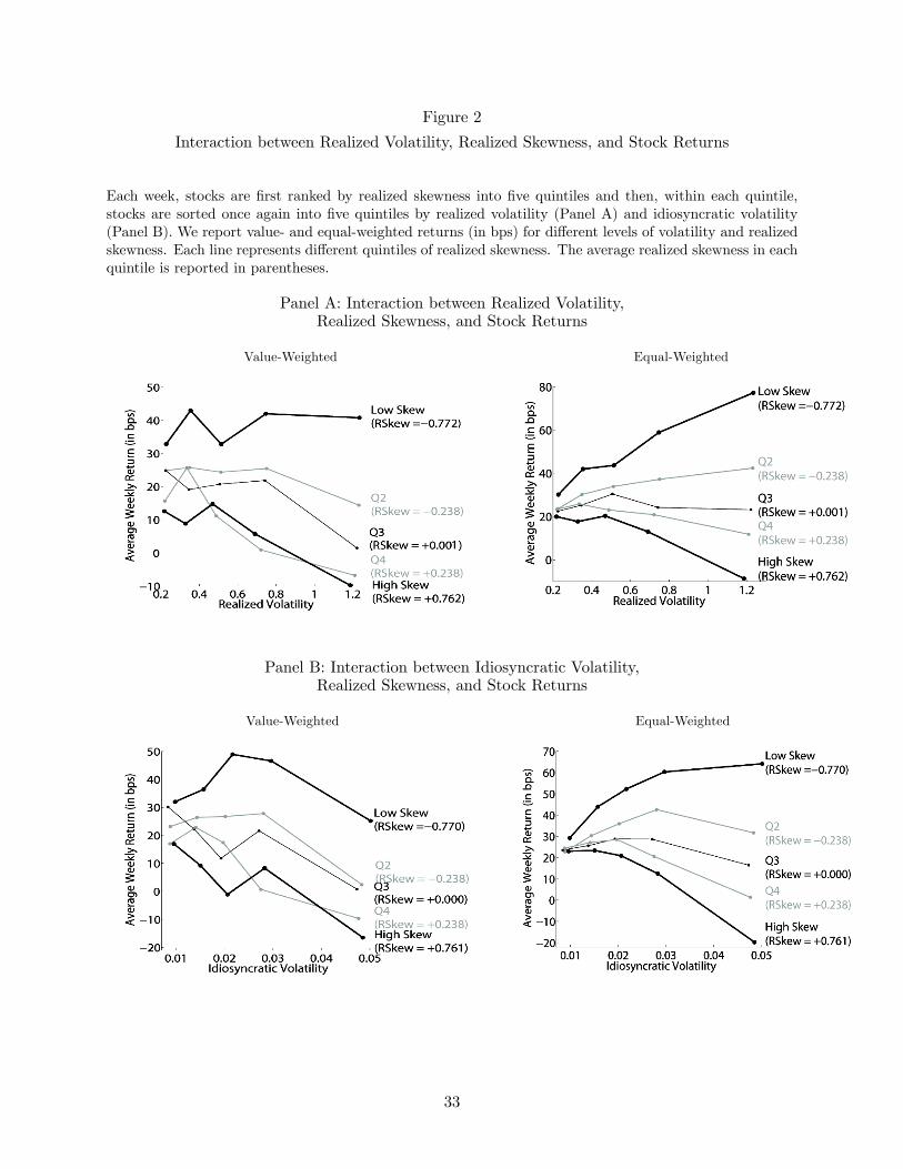
Figure 2

Interaction between Realized Volatility, Realized Skewness, and Stock Returns

Each week, stocks are �rst ranked by realized skewness into �ve quintiles and then, within each quintile,stocks are sorted once again into �ve quintiles by realized volatility (Panel A) and idiosyncratic volatility(Panel B). We report value- and equal-weighted returns (in bps) for di¤erent levels of volatility and realizedskewness. Each line represents di¤erent quintiles of realized skewness. The average realized skewness in eachquintile is reported in parentheses.

Panel A: Interaction between Realized Volatility,Realized Skewness, and Stock Returns

Value-Weighted Equal-Weighted

Panel B: Interaction between Idiosyncratic Volatility,Realized Skewness, and Stock Returns

Value-Weighted Equal-Weighted

33

Figure 3Signature Plots for Realized Moments

We show signature plots for the three daily realized moments, RM(2), RM(3), and RM(4) computedusing equation (12). The intraday sampling frequency on the horizontal axis is in seconds. The dottedlines represent the theoretical limit of realized moments as given by equations (14), (15), and (16). MonteCarlo estimates are plotted in continuous dark lines. Con�dence intervals at 99% are shown in grey lines.In Panel A, observed prices have a microstructure noise component, which is simulated from a mean-zeronormal distribution with a standard deviation of 0:05%. In Panel B, prices are only observed in sixteenthsof a dollar.

Panel A: Panel B:Market Microstructure Noise Discrete Price Changes

1 2 5 10 30 60 120 24000.002

0.006

0.010

0.014Second Moment

Sampling Frequency

Monte Carlo EstimateTheoretical LimitConfidence Interval

1 2 5 10 30 60 120 24000.002

0.006

0.010

0.014Second Moment

Sampling Frequency

Monte Carlo EstimateTheoretical LimitConfidence Interval

1 2 5 10 30 60 120 2402.3

2.8

3.4

4 x 10­5 Third Moment

Sampling Frequency

Monte Carlo EstimateTheoretical LimitConfidence Interval

1 2 5 10 30 60 120 2402.3

2.8

3.4

4 x 10­5 Third Moment

Sampling Frequency

Monte Carlo EstimateTheoretical LimitConfidence Interval

1 2 5 10 30 60 120 2407

7.5

8

8.5

9

x 10­6 Fourth Moment

Sampling Frequency

Monte Carlo EstimateTheoretical LimitConfidence Interval

1 2 5 10 30 60 120 2407

7.5

8

8.5

9

x 10­6 Fourth Moment

Sampling Frequency

Monte Carlo EstimateTheoretical LimitConfidence Interval

34

Table 1Characteristics of Portfolios Sorted by Realized Moments

Each week, stocks are ranked by their realized moment and sorted into deciles. The equal-weighted charac-teristics of those deciles are computed over the same week. This procedure is repeated for every week fromJanuary 1993 through September 2008. Panel A displays the average results for realized volatility, Panel Bfor realized skewness, and Panel C for realized kurtosis. Average characteristics of the portfolios are reportedfor the realized moment, Size ($ market capitalization in $billions), BE/ME (book-to-market equity ratio),Realized volatility (weekly realized volatility computed with high-frequency data), Historical Skewness (onemonth historical skewness from daily returns), Market Beta, Lagged Return, Idiosyncratic Volatility (com-puted as in Ang, Hodrick, Xing, and Zhang (2006)), Coskewness (computed as in Harvey and Siddique(2000)), Maximum Return (of the previous month), Illiquidity (annual average of the absolute return overdaily dollar trading volume times 106, as in Amihud (2002)), Number of Analysts (from I/B/E/S), CreditRating (1= AAA, 8= BBB+, 17= CCC+, 22=D), Price (stock price), Intraday Transactions (intradaytransactions per day) and Number of Stocks.

Panel A: Characteristics of Portfolios Sorted by Realized Volatility

Deciles 1 2 3 4 5 6 7 8 9 10

Realized Volatility 0.188 0.254 0.308 0.369 0.447 0.543 0.660 0.803 1.001 1.450Realized Skewness 0.024 0.020 0.012 0.004 0.000 -0.004 -0.009 -0.014 -0.024 -0.026Realized Kurtosis 7.0 6.9 7.0 7.2 7.5 7.8 8.1 8.4 8.8 9.4

Size 13.84 12.14 9.04 6.19 4.26 2.89 1.91 1.21 0.79 0.46BE/ME 0.654 0.573 0.509 0.507 0.488 0.459 0.428 0.421 0.417 0.440

Historical Skewness 0.109 0.102 0.109 0.126 0.144 0.166 0.191 0.212 0.241 0.311Market Beta 0.72 0.82 0.89 0.97 1.07 1.18 1.28 1.36 1.36 1.32

Lagged Return 0.003 0.004 0.004 0.005 0.005 0.006 0.007 0.008 0.010 0.028Idiosyncratic Volatility 0.011 0.013 0.015 0.017 0.020 0.023 0.027 0.031 0.036 0.048

Coskewness 0.003 -0.007 -0.018 -0.028 -0.032 -0.035 -0.041 -0.045 -0.049 -0.050Maximum Return 0.032 0.036 0.041 0.047 0.055 0.064 0.074 0.085 0.099 0.137

Illiquidity 0.005 0.005 0.006 0.009 0.013 0.020 0.035 0.080 0.126 0.562Number of Analysts 10.0 10.6 10.2 9.5 8.8 7.9 6.9 5.8 4.7 3.2

Credit Rating 7.0 7.4 7.9 8.4 8.7 8.9 8.9 8.8 8.7 8.4Price 62.2 53.6 38.9 33.5 29.6 27.7 24.7 21.4 17.8 15.0

Intraday Transactions 1,216 1,499 1,576 1,568 1,628 1,617 1,558 1,438 1,268 1,189Number of Stocks 256 257 257 257 257 257 257 257 257 257

35

Table 1 (Continued)

Panel B: Characteristics of Portfolios Sorted by Realized Skewness

Deciles 1 2 3 4 5 6 7 8 9 10

Realized Skewness -1.04 -0.50 -0.31 -0.17 -0.05 0.05 0.17 0.31 0.50 1.02Realized Volatility 0.618 0.613 0.614 0.614 0.610 0.606 0.600 0.590 0.577 0.579Realized Kurtosis 11.4 7.9 7.0 6.6 6.4 6.4 6.6 7.0 7.8 11.1

Size 2.96 4.41 5.22 5.75 6.22 6.22 6.09 5.69 4.91 3.49BE/ME 0.476 0.471 0.480 0.483 0.486 0.488 0.500 0.495 0.488 0.490

Historical Skewness 0.140 0.160 0.163 0.167 0.162 0.167 0.171 0.173 0.184 0.209Market Beta 1.05 1.14 1.12 1.11 1.09 1.10 1.11 1.11 1.10 1.02

Lagged Return -0.041 -0.025 -0.014 -0.006 0.003 0.011 0.020 0.030 0.042 0.061Idiosyncratic Volatility 0.026 0.025 0.024 0.024 0.023 0.023 0.023 0.024 0.024 0.025

Coskewness -0.038 -0.031 -0.028 -0.029 -0.027 -0.026 -0.025 -0.024 -0.025 -0.027Maximum Return 0.067 0.067 0.066 0.065 0.065 0.065 0.066 0.068 0.069 0.072

Illiquidity 0.116 0.071 0.082 0.066 0.076 0.059 0.058 0.067 0.102 0.158Number of Analysts 6.5 7.6 7.9 8.1 8.1 8.1 8.2 8.2 8.0 6.9

Credit Rating 8.4 8.3 8.3 8.3 8.3 8.3 8.3 8.3 8.3 8.4Price 29.8 32.6 33.2 32.2 31.5 31.4 33.0 33.7 33.9 33.1

Intraday Transactions 998 1,324 1,516 1,613 1,676 1,683 1,633 1,595 1,426 1,095Number of Stocks 256 257 257 257 257 257 257 257 257 257

Panel C: Characteristics of Portfolios Sorted by Realized Kurtosis

Deciles 1 2 3 4 5 6 7 8 9 10

Realized Kurtosis 3.9 4.7 5.3 5.9 6.5 7.2 8.0 9.2 10.9 16.6Realized Volatility 0.485 0.537 0.570 0.589 0.603 0.614 0.623 0.638 0.654 0.711Realized Skewness 0.005 0.007 0.006 0.006 0.007 0.003 0.000 -0.006 -0.012 -0.034

Size 15.59 8.80 6.22 4.89 3.88 3.27 2.80 2.38 1.98 1.36BE/ME 0.481 0.492 0.476 0.502 0.477 0.478 0.476 0.480 0.480 0.514Hskew 0.129 0.149 0.156 0.165 0.170 0.166 0.180 0.177 0.186 0.220Beta 1.09 1.15 1.16 1.15 1.14 1.13 1.12 1.08 1.03 0.90

Lagged Return 0.004 0.006 0.007 0.007 0.008 0.008 0.008 0.008 0.009 0.015Idiosyncratic Volatility 0.019 0.022 0.023 0.024 0.024 0.025 0.025 0.026 0.026 0.027

Coskewness -0.012 -0.017 -0.020 -0.023 -0.027 -0.030 -0.031 -0.036 -0.040 -0.046Maximum Return 0.053 0.061 0.065 0.067 0.068 0.069 0.070 0.070 0.071 0.076

Illiquidity 0.014 0.029 0.035 0.046 0.061 0.070 0.074 0.109 0.112 0.306Number of Analysts 11.4 10.1 9.1 8.4 7.8 7.4 6.9 6.4 5.8 4.4

Credit Rating 7.8 8.1 8.3 8.3 8.4 8.4 8.4 8.5 8.5 8.5Price 36.4 37.9 36.2 34.0 33.6 32.4 30.2 29.5 28.6 25.6

Intraday Transactions 3,250 2,195 1,795 1,553 1,349 1,217 1,067 917 736 483Number of Stocks 256 257 257 257 257 257 257 257 257 257

36

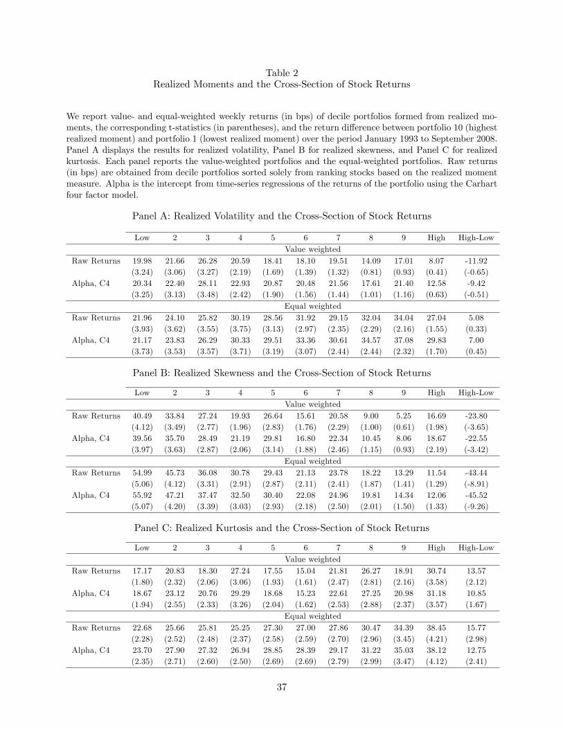
Table 2Realized Moments and the Cross-Section of Stock Returns

We report value- and equal-weighted weekly returns (in bps) of decile portfolios formed from realized mo-ments, the corresponding t-statistics (in parentheses), and the return di¤erence between portfolio 10 (highestrealized moment) and portfolio 1 (lowest realized moment) over the period January 1993 to September 2008.Panel A displays the results for realized volatility, Panel B for realized skewness, and Panel C for realizedkurtosis. Each panel reports the value-weighted portfolios and the equal-weighted portfolios. Raw returns(in bps) are obtained from decile portfolios sorted solely from ranking stocks based on the realized momentmeasure. Alpha is the intercept from time-series regressions of the returns of the portfolio using the Carhartfour factor model.

Panel A: Realized Volatility and the Cross-Section of Stock Returns

Low 2 3 4 5 6 7 8 9 High High-LowValue weighted

Raw Returns 19.98 21.66 26.28 20.59 18.41 18.10 19.51 14.09 17.01 8.07 -11.92(3.24) (3.06) (3.27) (2.19) (1.69) (1.39) (1.32) (0.81) (0.93) (0.41) (-0.65)

Alpha, C4 20.34 22.40 28.11 22.93 20.87 20.48 21.56 17.61 21.40 12.58 -9.42(3.25) (3.13) (3.48) (2.42) (1.90) (1.56) (1.44) (1.01) (1.16) (0.63) (-0.51)

Equal weightedRaw Returns 21.96 24.10 25.82 30.19 28.56 31.92 29.15 32.04 34.04 27.04 5.08

(3.93) (3.62) (3.55) (3.75) (3.13) (2.97) (2.35) (2.29) (2.16) (1.55) (0.33)Alpha, C4 21.17 23.83 26.29 30.33 29.51 33.36 30.61 34.57 37.08 29.83 7.00

(3.73) (3.53) (3.57) (3.71) (3.19) (3.07) (2.44) (2.44) (2.32) (1.70) (0.45)

Panel B: Realized Skewness and the Cross-Section of Stock Returns

Low 2 3 4 5 6 7 8 9 High High-LowValue weighted

Raw Returns 40.49 33.84 27.24 19.93 26.64 15.61 20.58 9.00 5.25 16.69 -23.80(4.12) (3.49) (2.77) (1.96) (2.83) (1.76) (2.29) (1.00) (0.61) (1.98) (-3.65)

Alpha, C4 39.56 35.70 28.49 21.19 29.81 16.80 22.34 10.45 8.06 18.67 -22.55(3.97) (3.63) (2.87) (2.06) (3.14) (1.88) (2.46) (1.15) (0.93) (2.19) (-3.42)

Equal weightedRaw Returns 54.99 45.73 36.08 30.78 29.43 21.13 23.78 18.22 13.29 11.54 -43.44

(5.06) (4.12) (3.31) (2.91) (2.87) (2.11) (2.41) (1.87) (1.41) (1.29) (-8.91)Alpha, C4 55.92 47.21 37.47 32.50 30.40 22.08 24.96 19.81 14.34 12.06 -45.52

(5.07) (4.20) (3.39) (3.03) (2.93) (2.18) (2.50) (2.01) (1.50) (1.33) (-9.26)

Panel C: Realized Kurtosis and the Cross-Section of Stock Returns

Low 2 3 4 5 6 7 8 9 High High-LowValue weighted

Raw Returns 17.17 20.83 18.30 27.24 17.55 15.04 21.81 26.27 18.91 30.74 13.57(1.80) (2.32) (2.06) (3.06) (1.93) (1.61) (2.47) (2.81) (2.16) (3.58) (2.12)

Alpha, C4 18.67 23.12 20.76 29.29 18.68 15.23 22.61 27.25 20.98 31.18 10.85(1.94) (2.55) (2.33) (3.26) (2.04) (1.62) (2.53) (2.88) (2.37) (3.57) (1.67)

Equal weightedRaw Returns 22.68 25.66 25.81 25.25 27.30 27.00 27.86 30.47 34.39 38.45 15.77

(2.28) (2.52) (2.48) (2.37) (2.58) (2.59) (2.70) (2.96) (3.45) (4.21) (2.98)Alpha, C4 23.70 27.90 27.32 26.94 28.85 28.39 29.17 31.22 35.03 38.12 12.75

(2.35) (2.71) (2.60) (2.50) (2.69) (2.69) (2.79) (2.99) (3.47) (4.12) (2.41)

37

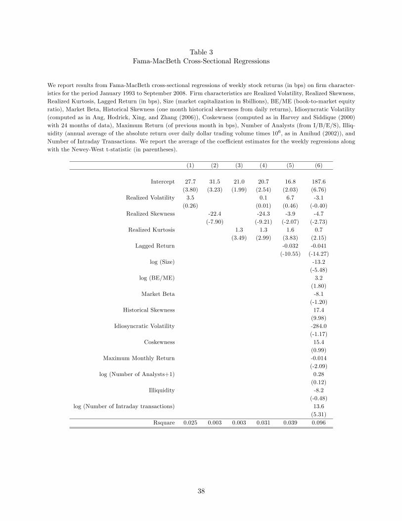
Table 3Fama-MacBeth Cross-Sectional Regressions

We report results from Fama-MacBeth cross-sectional regressions of weekly stock returns (in bps) on �rm character-istics for the period January 1993 to September 2008. Firm characteristics are Realized Volatility, Realized Skewness,Realized Kurtosis, Lagged Return (in bps), Size (market capitalization in $billions), BE/ME (book-to-market equityratio), Market Beta, Historical Skewness (one month historical skewness from daily returns), Idiosyncratic Volatility(computed as in Ang, Hodrick, Xing, and Zhang (2006)), Coskewness (computed as in Harvey and Siddique (2000)with 24 months of data), Maximum Return (of previous month in bps), Number of Analysts (from I/B/E/S), Illiq-uidity (annual average of the absolute return over daily dollar trading volume times 106, as in Amihud (2002)), andNumber of Intraday Transactions. We report the average of the coe¢ cient estimates for the weekly regressions alongwith the Newey-West t-statistic (in parentheses).

(1) (2) (3) (4) (5) (6)

Intercept 27.7 31.5 21.0 20.7 16.8 187.6(3.80) (3.23) (1.99) (2.54) (2.03) (6.76)

Realized Volatility 3.5 0.1 6.7 -3.1(0.26) (0.01) (0.46) (-0.40)

Realized Skewness -22.4 -24.3 -3.9 -4.7(-7.90) (-9.21) (-2.07) (-2.73)

Realized Kurtosis 1.3 1.3 1.6 0.7(3.49) (2.99) (3.83) (2.15)

Lagged Return -0.032 -0.041(-10.55) (-14.27)

log (Size) -13.2(-5.48)

log (BE/ME) 3.2(1.80)

Market Beta -8.1(-1.20)

Historical Skewness 17.4(9.98)

Idiosyncratic Volatility -284.0(-1.17)

Coskewness 15.4(0.99)

Maximum Monthly Return -0.014(-2.09)

log (Number of Analysts+1) 0.28(0.12)

Illiquidity -8.2(-0.48)

log (Number of Intraday transactions) 13.6(5.31)

Rsquare 0.025 0.003 0.003 0.031 0.039 0.096

38

Table 4Double Sorting on Realized Skewness and Realized Volatility

Each week, stocks are �rst sorted by realized skewness into �ve quintiles and then, within each quintile,stocks are sorted once again into �ve quintiles by realized volatility. Panel A reports value-weighted returnsand Panel B reports equal-weighted returns. The value- and equal-weighted average weekly returns (in bps)are reported for all double sorted portfolios as well as for the di¤erence between portfolio �ve (High volatility)and one (Low volatility) for each level of realized skewness. T-statistics are in parentheses.

Panel A: Value-WeightedLow 2 3 4 High High-Low RVol

1 (Low Realized Skewness) 32.7 43.1 32.7 42.0 40.8 8.1(4.32) (4.47) (2.45) (2.47) (2.07) (0.46)

2 25.0 25.6 24.1 25.6 14.8 -10.2(3.40) (2.70) (1.82) (1.50) (0.70) (-0.55)

3 24.9 19.1 20.8 21.5 1.1 -23.7(3.59) (2.11) (1.68) (1.35) (0.06) (-1.35)

4 15.4 25.5 10.6 0.7 -6.9 -22.2(2.27) (2.96) (0.88) (0.04) (-0.35) (-1.25)

5 (High Realized Skewness) 12.6 8.7 14.6 6.1 -9.6 -22.2(1.89) (0.95) (1.34) (0.44) (-0.53) (-1.34)

Panel B: Equal-WeightedLow 2 3 4 High High-Low RVol

1 (Low Realized Skewness) 30.0 42.0 43.2 59.0 77.0 47.2(4.50) (4.92) (3.70) (4.16) (4.47) (3.31)

2 23.8 30.2 33.5 37.2 43.0 18.9(3.73) (3.74) (3.09) (2.61) (2.37) (1.23)

3 22.5 25.3 30.0 24.2 23.0 0.6(3.70) (3.28) (3.02) (1.77) (1.36) (0.04)

4 23.4 25.3 23.1 20.8 12.0 -11.7(3.88) (3.33) (2.40) (1.60) (0.70) (-0.80)

5 (High Realized Skewness) 19.9 17.6 20.2 13.0 -9.0 -28.4(3.32) (2.33) (2.20) (1.09) (-0.56) (-2.22)

39

Table 5Idiosyncratic Volatility and the Cross-Section of Stock Returns

We report value- and equal-weighted weekly returns (in bps) of quintile portfolios ranked by idiosyncraticvolatility, their t-statistics (in parentheses), and the di¤erence between portfolio 5 (highest idiosyncraticvolatility) and portfolio 1 (lowest idiosyncratic volatility) over the period January 1993 to September 2008.Panel A reports on value-weighted portfolios and Panel B reports on equal-weighted portfolios. Raw returns(in bps) are obtained for quintile portfolios sorted solely on the idiosyncratic volatility measure. Alpha isthe intercept from the time-series regressions for the return on the portfolio that buys portfolio 5 and sellsportfolio 1, using the Carhart four-factor model.

Panel A: Value-Weighted

Low 2 3 4 High High-Low

Raw Returns 24.61 22.76 15.05 18.40 0.48 -24.14(3.46) (2.79) (1.46) (1.39) (0.03) (-1.73)

Alpha, C4 25.95 24.54 16.36 21.71 5.09 -22.53(3.63) (2.99) (1.57) (1.62) (0.30) (-1.59)

Panel B: Equal-Weighted

Low 2 3 4 High High-LowRaw Returns 23.61 30.38 32.69 32.23 20.96 -2.64

(3.96) (3.96) (3.30) (2.50) (1.30) (-0.20)Alpha, C4 23.59 30.91 33.50 34.64 23.11 -2.14

(3.91) (3.98) (3.34) (2.65) (1.42) (-0.16)

40

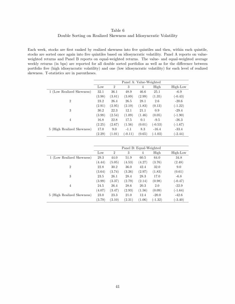
Table 6Double Sorting on Realized Skewness and Idiosyncratic Volatility

Each week, stocks are �rst ranked by realized skewness into �ve quintiles and then, within each quintile,stocks are sorted once again into �ve quintiles based on idiosyncratic volatility. Panel A reports on value-weighted returns and Panel B reports on equal-weighted returns. The value- and equal-weighted averageweekly returns (in bps) are reported for all double sorted portfolios as well as for the di¤erence betweenportfolio �ve (high idiosyncratic volatility) and one (low idiosyncratic volatility) for each level of realizedskewness. T-statistics are in parentheses.

Panel A: Value-WeightedLow 2 3 4 High High-Low

1 (Low Realized Skewness) 32.1 36.1 48.9 46.6 25.1 -6.9(3.98) (3.81) (3.89) (2.99) (1.35) (-0.43)

2 23.2 26.4 26.5 28.1 2.6 -20.6(2.91) (2.95) (2.19) (1.83) (0.13) (-1.22)

3 30.2 22.3 12.1 21.1 0.9 -29.4(3.98) (2.54) (1.09) (1.46) (0.05) (-1.90)

4 16.8 22.8 17.5 0.1 -9.5 -26.3(2.25) (2.67) (1.56) (0.01) (-0.53) (-1.67)

5 (High Realized Skewness) 17.0 9.0 -1.1 8.3 -16.4 -33.4(2.29) (1.01) (-0.11) (0.65) (-1.03) (-2.44)

Panel B: Equal-WeightedLow 2 3 4 High High-Low

1 (Low Realized Skewness) 29.3 44.0 51.9 60.5 64.0 34.8(4.44) (5.05) (4.53) (4.27) (3.76) (2.48)

2 22.8 30.2 36.0 42.4 32.0 9.0(3.64) (3.74) (3.26) (2.97) (1.83) (0.61)

3 23.5 26.1 28.4 28.3 17.0 -6.8(3.99) (3.37) (2.79) (2.14) (0.98) (-0.47)

4 24.5 26.4 28.6 20.3 2.0 -22.9(4.07) (3.47) (2.93) (1.56) (0.09) (-1.64)

5 (High Realized Skewness) 23.0 23.3 21.0 12.4 -20.0 -42.6(3.79) (3.10) (2.31) (1.06) (-1.32) (-3.40)

41

Table 7Realized Moments and Returns for Di¤erent Subsamples

We report weekly returns (in bps) and t-statistics of quintile portfolios formed from ranking stocks by theirrealized moments. We also report the di¤erence between portfolio 5 (highest realized moment) and portfolio1 (lowest realized moment). Panel A displays results for realized skewness and Panel B for realized kurtosis.Each panel reports the value- and equal-weighted quintile portfolio returns for the month of January, for allmonths excluding January, and only for NYSE stocks.

Panel A: Realized Skewness E¤ects for Di¤erent Subsamples

Value weightedLow 2 3 4 High High-Low

Raw Returns, January 54.76 43.49 36.75 18.08 24.20 -30.57(2.11) (1.45) (1.43) (0.68) (0.90) (-1.72)

Raw Returns, Non-January 34.31 20.93 19.47 13.99 8.09 -26.22(3.41) (2.03) (2.08) (1.52) (0.93) (-4.80)

Raw Returns, NYSE 44.61 31.23 26.48 13.90 13.06 -31.55(3.08) (2.04) (1.82) (1.01) (1.02) (-3.51)

Equal weightedLow 2 3 4 High High-Low

Raw Returns, January 93.27 55.86 59.54 54.28 37.21 -56.05(2.72) (1.74) (1.98) (1.76) (1.31) (-4.13)

Raw Returns, Non-January 46.36 31.37 22.15 17.90 10.11 -36.25(4.05) (2.78) (2.08) (1.75) (1.06) (-8.36)

Raw Returns, NYSE 66.84 44.06 28.57 18.80 2.48 -64.36(4.81) (3.08) (2.06) (1.40) (0.21) (-12.27)

Panel B: Realized Kurtosis E¤ects for Di¤erent Subsamples

Value weightedLow 2 3 4 High High-Low

Raw Returns, January 31.25 38.43 37.81 30.27 58.70 27.44(1.20) (1.44) (1.38) (1.26) (2.10) (1.46)

Raw Returns, Non-January 17.49 21.28 13.61 23.45 19.44 1.95(1.82) (2.35) (1.45) (2.51) (2.24) (0.39)

Raw Returns, NYSE 25.41 22.47 16.71 33.42 32.15 6.75(1.75) (1.59) (1.24) (2.71) (2.89) (0.75)

Equal weightedLow 2 3 4 High High-Low

Raw Returns, January 47.14 58.03 63.79 60.40 70.76 23.62(1.54) (1.82) (1.97) (1.93) (2.34) (1.59)

Raw Returns, Non-January 22.05 22.56 23.74 26.26 33.23 11.18(2.10) (2.05) (2.16) (2.44) (3.35) (2.66)

Raw Returns, NYSE 25.85 31.95 28.70 33.81 40.34 14.49(1.63) (2.16) (2.11) (2.67) (3.72) (1.88)

42

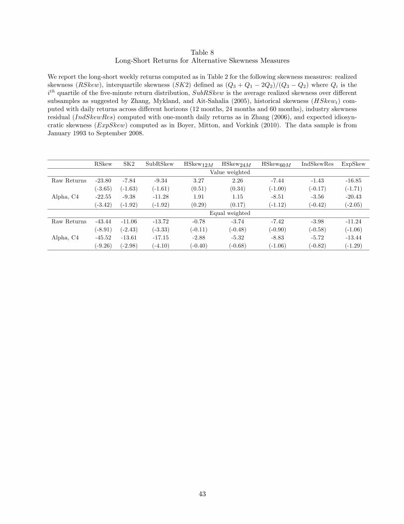
Table 8Long-Short Returns for Alternative Skewness Measures

We report the long-short weekly returns computed as in Table 2 for the following skewness measures: realizedskewness (RSkew), interquartile skewness (SK2) de�ned as (Q3 + Q1 � 2Q2)=(Q3 � Q2) where Qi is theith quartile of the �ve-minute return distribution, SubRSkew is the average realized skewness over di¤erentsubsamples as suggested by Zhang, Mykland, and Ait-Sahalia (2005), historical skewness (HSkewt) com-puted with daily returns across di¤erent horizons (12 months, 24 months and 60 months), industry skewnessresidual (IndSkewRes) computed with one-month daily returns as in Zhang (2006), and expected idiosyn-cratic skewness (ExpSkew) computed as in Boyer, Mitton, and Vorkink (2010). The data sample is fromJanuary 1993 to September 2008.

RSkew SK2 SubRSkew HSkew12M HSkew24M HSkew60M IndSkewRes ExpSkewValue weighted

Raw Returns -23.80 -7.84 -9.34 3.27 2.26 -7.44 -1.43 -16.85(-3.65) (-1.63) (-1.61) (0.51) (0.34) (-1.00) (-0.17) (-1.71)

Alpha, C4 -22.55 -9.38 -11.28 1.91 1.15 -8.51 -3.56 -20.43(-3.42) (-1.92) (-1.92) (0.29) (0.17) (-1.12) (-0.42) (-2.05)

Equal weightedRaw Returns -43.44 -11.06 -13.72 -0.78 -3.74 -7.42 -3.98 -11.24

(-8.91) (-2.43) (-3.33) (-0.11) (-0.48) (-0.90) (-0.58) (-1.06)Alpha, C4 -45.52 -13.61 -17.15 -2.88 -5.32 -8.83 -5.72 -13.44

(-9.26) (-2.98) (-4.10) (-0.40) (-0.68) (-1.06) (-0.82) (-1.29)

43

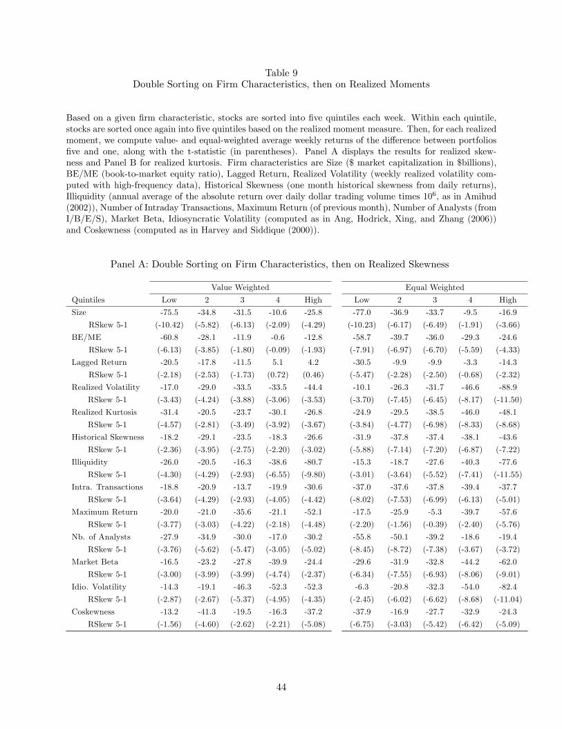
Table 9Double Sorting on Firm Characteristics, then on Realized Moments

Based on a given �rm characteristic, stocks are sorted into �ve quintiles each week. Within each quintile,stocks are sorted once again into �ve quintiles based on the realized moment measure. Then, for each realizedmoment, we compute value- and equal-weighted average weekly returns of the di¤erence between portfolios�ve and one, along with the t-statistic (in parentheses). Panel A displays the results for realized skew-ness and Panel B for realized kurtosis. Firm characteristics are Size ($ market capitalization in $billions),BE/ME (book-to-market equity ratio), Lagged Return, Realized Volatility (weekly realized volatility com-puted with high-frequency data), Historical Skewness (one month historical skewness from daily returns),Illiquidity (annual average of the absolute return over daily dollar trading volume times 106, as in Amihud(2002)), Number of Intraday Transactions, Maximum Return (of previous month), Number of Analysts (fromI/B/E/S), Market Beta, Idiosyncratic Volatility (computed as in Ang, Hodrick, Xing, and Zhang (2006))and Coskewness (computed as in Harvey and Siddique (2000)).

Panel A: Double Sorting on Firm Characteristics, then on Realized Skewness

Value Weighted Equal Weighted

Quintiles Low 2 3 4 High Low 2 3 4 High

Size -75.5 -34.8 -31.5 -10.6 -25.8 -77.0 -36.9 -33.7 -9.5 -16.9

RSkew 5-1 (-10.42) (-5.82) (-6.13) (-2.09) (-4.29) (-10.23) (-6.17) (-6.49) (-1.91) (-3.66)

BE/ME -60.8 -28.1 -11.9 -0.6 -12.8 -58.7 -39.7 -36.0 -29.3 -24.6

RSkew 5-1 (-6.13) (-3.85) (-1.80) (-0.09) (-1.93) (-7.91) (-6.97) (-6.70) (-5.59) (-4.33)

Lagged Return -20.5 -17.8 -11.5 5.1 4.2 -30.5 -9.9 -9.9 -3.3 -14.3

RSkew 5-1 (-2.18) (-2.53) (-1.73) (0.72) (0.46) (-5.47) (-2.28) (-2.50) (-0.68) (-2.32)

Realized Volatility -17.0 -29.0 -33.5 -33.5 -44.4 -10.1 -26.3 -31.7 -46.6 -88.9

RSkew 5-1 (-3.43) (-4.24) (-3.88) (-3.06) (-3.53) (-3.70) (-7.45) (-6.45) (-8.17) (-11.50)

Realized Kurtosis -31.4 -20.5 -23.7 -30.1 -26.8 -24.9 -29.5 -38.5 -46.0 -48.1

RSkew 5-1 (-4.57) (-2.81) (-3.49) (-3.92) (-3.67) (-3.84) (-4.77) (-6.98) (-8.33) (-8.68)

Historical Skewness -18.2 -29.1 -23.5 -18.3 -26.6 -31.9 -37.8 -37.4 -38.1 -43.6

RSkew 5-1 (-2.36) (-3.95) (-2.75) (-2.20) (-3.02) (-5.88) (-7.14) (-7.20) (-6.87) (-7.22)

Illiquidity -26.0 -20.5 -16.3 -38.6 -80.7 -15.3 -18.7 -27.6 -40.3 -77.6

RSkew 5-1 (-4.30) (-4.29) (-2.93) (-6.55) (-9.80) (-3.01) (-3.64) (-5.52) (-7.41) (-11.55)

Intra. Transactions -18.8 -20.9 -13.7 -19.9 -30.6 -37.0 -37.6 -37.8 -39.4 -37.7

RSkew 5-1 (-3.64) (-4.29) (-2.93) (-4.05) (-4.42) (-8.02) (-7.53) (-6.99) (-6.13) (-5.01)

Maximum Return -20.0 -21.0 -35.6 -21.1 -52.1 -17.5 -25.9 -5.3 -39.7 -57.6

RSkew 5-1 (-3.77) (-3.03) (-4.22) (-2.18) (-4.48) (-2.20) (-1.56) (-0.39) (-2.40) (-5.76)

Nb. of Analysts -27.9 -34.9 -30.0 -17.0 -30.2 -55.8 -50.1 -39.2 -18.6 -19.4

RSkew 5-1 (-3.76) (-5.62) (-5.47) (-3.05) (-5.02) (-8.45) (-8.72) (-7.38) (-3.67) (-3.72)

Market Beta -16.5 -23.2 -27.8 -39.9 -24.4 -29.6 -31.9 -32.8 -44.2 -62.0

RSkew 5-1 (-3.00) (-3.99) (-3.99) (-4.74) (-2.37) (-6.34) (-7.55) (-6.93) (-8.06) (-9.01)

Idio. Volatility -14.3 -19.1 -46.3 -52.3 -52.3 -6.3 -20.8 -32.3 -54.0 -82.4

RSkew 5-1 (-2.87) (-2.67) (-5.37) (-4.95) (-4.35) (-2.45) (-6.02) (-6.62) (-8.68) (-11.04)

Coskewness -13.2 -41.3 -19.5 -16.3 -37.2 -37.9 -16.9 -27.7 -32.9 -24.3

RSkew 5-1 (-1.56) (-4.60) (-2.62) (-2.21) (-5.08) (-6.75) (-3.03) (-5.42) (-6.42) (-5.09)

44

Table 9 (Continued)

Panel B: Double Sorting on Firm Characteristics, then on Realized Kurtosis

Characteristics - Value Weighted Characteristics - Equal Weighted

Quintiles Low 2 3 4 High Low 2 3 4 High

Size -0.8 10.7 1.9 -1.1 4.0 4.3 12.1 1.8 -1.0 -0.6

RKurt 5-1 (-0.08) (1.36) (0.32) (-0.22) (0.78) (0.42) (1.53) (0.31) (-0.19) (-0.13)

BE/ME 4.5 -0.7 0.4 14.5 0.4 14.3 -3.6 9.5 11.6 21.4

RKurt 5-1 (0.49) (-0.09) (0.07) (2.47) (0.07) (2.05) (-0.61) (1.83) (2.21) (3.54)

Lagged Return -11.7 -2.0 3.9 18.5 14.5 16.7 8.9 9.6 21.2 15.8

RKurt 5-1 (-1.16) (-0.28) (0.58) (2.68) (1.71) (2.10) (1.76) (2.28) (4.16) (2.24)

Realized Volatility 3.1 2.6 15.0 8.2 36.2 3.8 1.7 15.3 16.3 20.3

RKurt 5-1 (0.68) (0.39) (1.55) (0.67) (2.50) (1.22) (0.45) (2.82) (1.91) (1.88)

Realized Skewness 9.5 -2.5 2.7 4.6 10.7 14.1 7.2 13.1 9.5 8.5

RKurt 5-1 (1.14) (-0.33) (0.36) (0.62) (1.64) (2.28) (1.24) (2.27) (1.72) (1.65)

Historical Skewness 5.2 9.2 7.7 1.6 19.9 12.3 17.5 11.7 13.0 2.7

RKurt 5-1 (0.66) (1.43) (1.04) (0.19) (2.53) (2.34) (3.45) (2.20) (2.19) (0.41)

Illiquidity 6.1 -3.7 -4.8 4.0 4.6 3.7 0.6 2.5 2.6 12.6

RKurt 5-1 (1.13) (-0.84) (-0.84) (0.56) (0.44) (0.77) (0.12) (0.51) (0.40) (1.37)

Intra. Transactions 5.5 7.4 -2.3 7.3 5.1 25.1 17.7 13.1 11.4 -2.4

RKurt 5-1 (1.00) (1.41) (-0.43) (1.46) (0.78) (5.23) (3.48) (2.41) (1.84) (-0.35)

Maximum Return -8.3 15.1 9.0 23.9 5.1 14.3 11.5 30.0 28.1 -0.8

RKurt 5-1 (-1.51) (2.28) (1.18) (2.46) (0.41) (1.87) (0.45) (2.17) (1.61) (-0.08)

Nb. of Analysts 9.8 4.3 -1.9 3.0 2.3 17.9 5.9 3.6 -1.9 4.3

RKurt 5-1 (1.02) (0.63) (-0.34) (0.59) (0.41) (2.08) (0.92) (0.69) (-0.41) (0.82)

Market Beta 7.4 6.8 7.4 -0.3 -1.6 27.7 14.1 11.2 -0.8 -4.9

RKurt 5-1 (1.35) (1.12) (1.20) (-0.04) (-0.16) (5.32) (3.29) (2.34) (-0.15) (-0.68)

Idio. Volatility -4.1 9.3 16.8 5.9 18.4 3.5 9.0 10.9 19.4 19.7

RKurt 5-1 (-0.80) (1.42) (1.96) (0.57) (1.45) (1.17) (2.33) (2.08) (2.68) (2.04)

Coskewness 5.0 11.2 2.0 -0.6 4.0 13.5 17.1 4.1 10.8 5.2

RKurt 5-1 (0.62) (1.44) (0.27) (-0.09) (0.60) (2.17) (2.81) (0.80) (2.12) (1.08)

45

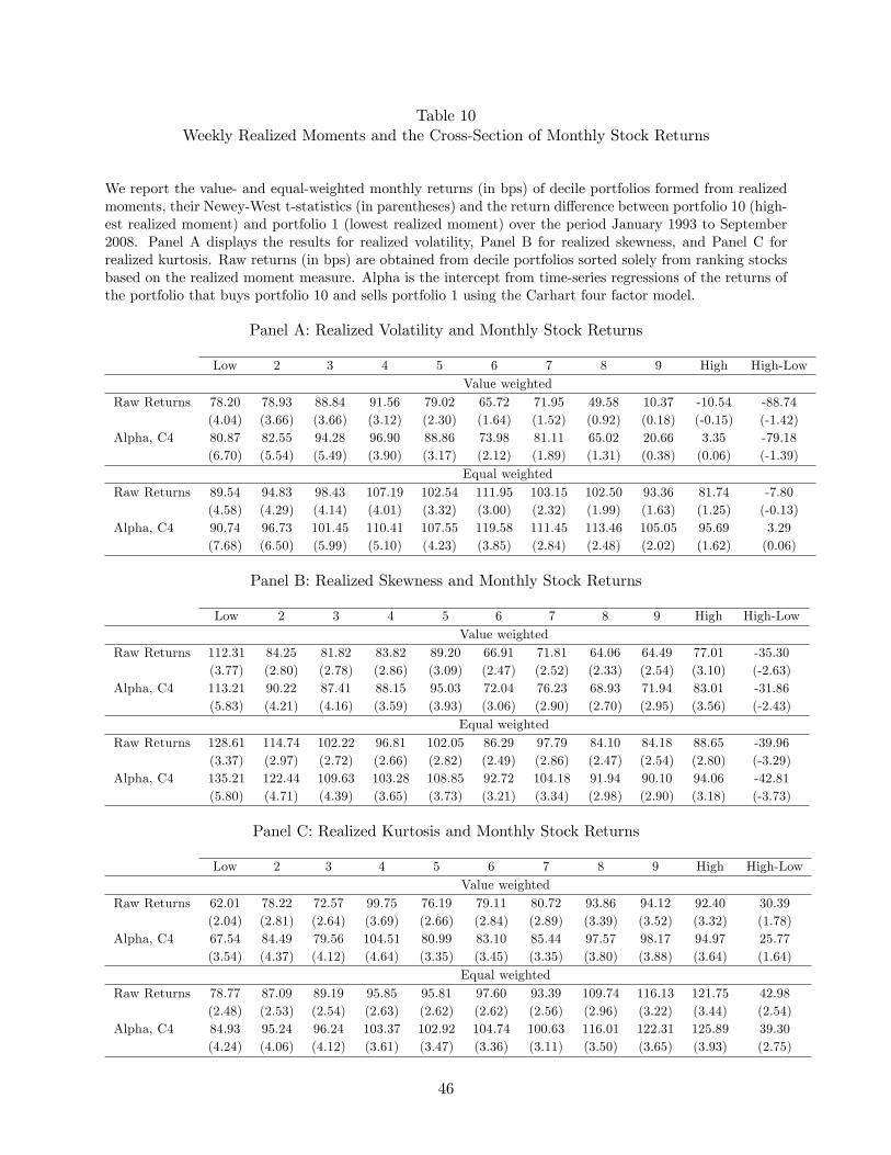
Table 10Weekly Realized Moments and the Cross-Section of Monthly Stock Returns

We report the value- and equal-weighted monthly returns (in bps) of decile portfolios formed from realizedmoments, their Newey-West t-statistics (in parentheses) and the return di¤erence between portfolio 10 (high-est realized moment) and portfolio 1 (lowest realized moment) over the period January 1993 to September2008. Panel A displays the results for realized volatility, Panel B for realized skewness, and Panel C forrealized kurtosis. Raw returns (in bps) are obtained from decile portfolios sorted solely from ranking stocksbased on the realized moment measure. Alpha is the intercept from time-series regressions of the returns ofthe portfolio that buys portfolio 10 and sells portfolio 1 using the Carhart four factor model.

Panel A: Realized Volatility and Monthly Stock Returns

Low 2 3 4 5 6 7 8 9 High High-LowValue weighted

Raw Returns 78.20 78.93 88.84 91.56 79.02 65.72 71.95 49.58 10.37 -10.54 -88.74(4.04) (3.66) (3.66) (3.12) (2.30) (1.64) (1.52) (0.92) (0.18) (-0.15) (-1.42)

Alpha, C4 80.87 82.55 94.28 96.90 88.86 73.98 81.11 65.02 20.66 3.35 -79.18(6.70) (5.54) (5.49) (3.90) (3.17) (2.12) (1.89) (1.31) (0.38) (0.06) (-1.39)

Equal weightedRaw Returns 89.54 94.83 98.43 107.19 102.54 111.95 103.15 102.50 93.36 81.74 -7.80

(4.58) (4.29) (4.14) (4.01) (3.32) (3.00) (2.32) (1.99) (1.63) (1.25) (-0.13)Alpha, C4 90.74 96.73 101.45 110.41 107.55 119.58 111.45 113.46 105.05 95.69 3.29

(7.68) (6.50) (5.99) (5.10) (4.23) (3.85) (2.84) (2.48) (2.02) (1.62) (0.06)

Panel B: Realized Skewness and Monthly Stock Returns

Low 2 3 4 5 6 7 8 9 High High-LowValue weighted

Raw Returns 112.31 84.25 81.82 83.82 89.20 66.91 71.81 64.06 64.49 77.01 -35.30(3.77) (2.80) (2.78) (2.86) (3.09) (2.47) (2.52) (2.33) (2.54) (3.10) (-2.63)

Alpha, C4 113.21 90.22 87.41 88.15 95.03 72.04 76.23 68.93 71.94 83.01 -31.86(5.83) (4.21) (4.16) (3.59) (3.93) (3.06) (2.90) (2.70) (2.95) (3.56) (-2.43)

Equal weightedRaw Returns 128.61 114.74 102.22 96.81 102.05 86.29 97.79 84.10 84.18 88.65 -39.96

(3.37) (2.97) (2.72) (2.66) (2.82) (2.49) (2.86) (2.47) (2.54) (2.80) (-3.29)Alpha, C4 135.21 122.44 109.63 103.28 108.85 92.72 104.18 91.94 90.10 94.06 -42.81

(5.80) (4.71) (4.39) (3.65) (3.73) (3.21) (3.34) (2.98) (2.90) (3.18) (-3.73)

Panel C: Realized Kurtosis and Monthly Stock Returns

Low 2 3 4 5 6 7 8 9 High High-LowValue weighted

Raw Returns 62.01 78.22 72.57 99.75 76.19 79.11 80.72 93.86 94.12 92.40 30.39(2.04) (2.81) (2.64) (3.69) (2.66) (2.84) (2.89) (3.39) (3.52) (3.32) (1.78)

Alpha, C4 67.54 84.49 79.56 104.51 80.99 83.10 85.44 97.57 98.17 94.97 25.77(3.54) (4.37) (4.12) (4.64) (3.35) (3.45) (3.35) (3.80) (3.88) (3.64) (1.64)

Equal weightedRaw Returns 78.77 87.09 89.19 95.85 95.81 97.60 93.39 109.74 116.13 121.75 42.98

(2.48) (2.53) (2.54) (2.63) (2.62) (2.62) (2.56) (2.96) (3.22) (3.44) (2.54)Alpha, C4 84.93 95.24 96.24 103.37 102.92 104.74 100.63 116.01 122.31 125.89 39.30

(4.24) (4.06) (4.12) (3.61) (3.47) (3.36) (3.11) (3.50) (3.65) (3.93) (2.75)

46

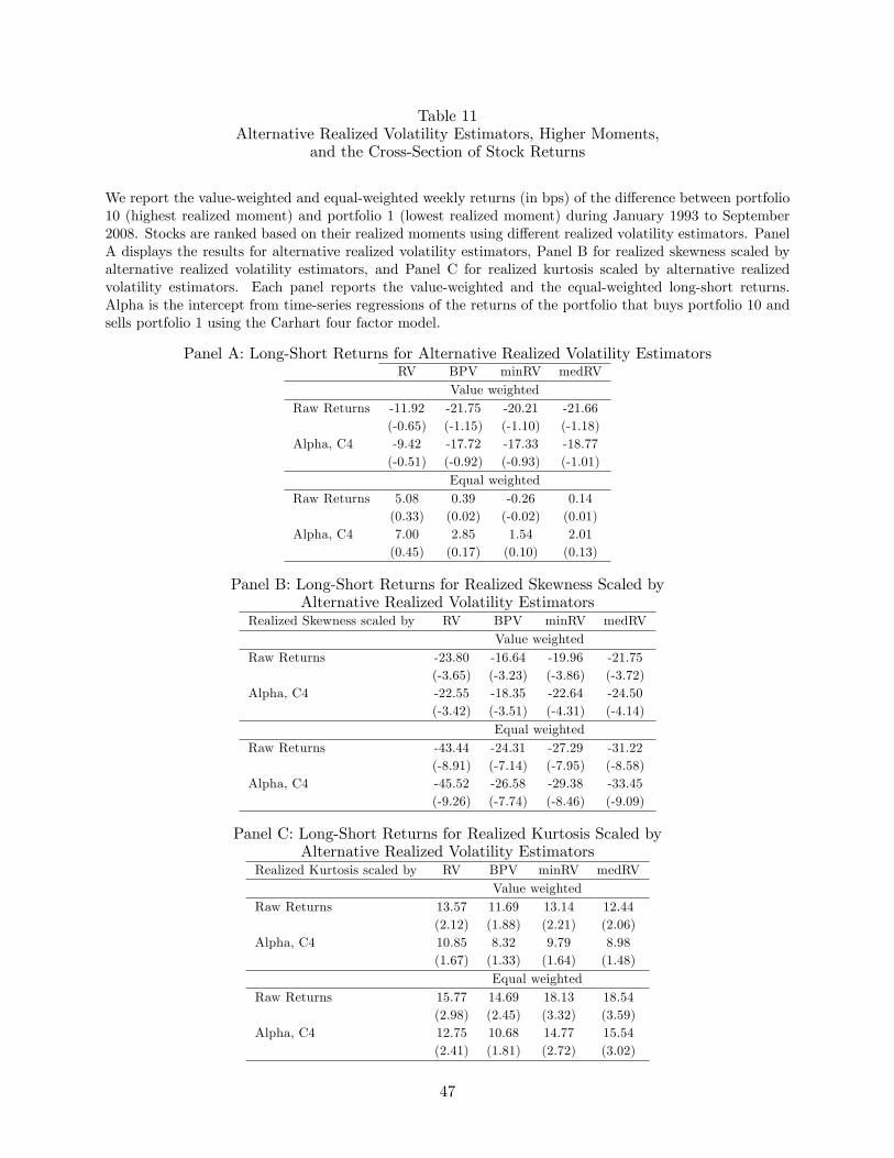
Table 11Alternative Realized Volatility Estimators, Higher Moments,

and the Cross-Section of Stock Returns

We report the value-weighted and equal-weighted weekly returns (in bps) of the di¤erence between portfolio10 (highest realized moment) and portfolio 1 (lowest realized moment) during January 1993 to September2008. Stocks are ranked based on their realized moments using di¤erent realized volatility estimators. PanelA displays the results for alternative realized volatility estimators, Panel B for realized skewness scaled byalternative realized volatility estimators, and Panel C for realized kurtosis scaled by alternative realizedvolatility estimators. Each panel reports the value-weighted and the equal-weighted long-short returns.Alpha is the intercept from time-series regressions of the returns of the portfolio that buys portfolio 10 andsells portfolio 1 using the Carhart four factor model.

Panel A: Long-Short Returns for Alternative Realized Volatility EstimatorsRV BPV minRV medRV

Value weightedRaw Returns -11.92 -21.75 -20.21 -21.66

(-0.65) (-1.15) (-1.10) (-1.18)Alpha, C4 -9.42 -17.72 -17.33 -18.77

(-0.51) (-0.92) (-0.93) (-1.01)Equal weighted

Raw Returns 5.08 0.39 -0.26 0.14(0.33) (0.02) (-0.02) (0.01)

Alpha, C4 7.00 2.85 1.54 2.01(0.45) (0.17) (0.10) (0.13)

Panel B: Long-Short Returns for Realized Skewness Scaled byAlternative Realized Volatility Estimators

Realized Skewness scaled by RV BPV minRV medRVValue weighted

Raw Returns -23.80 -16.64 -19.96 -21.75(-3.65) (-3.23) (-3.86) (-3.72)

Alpha, C4 -22.55 -18.35 -22.64 -24.50(-3.42) (-3.51) (-4.31) (-4.14)

Equal weightedRaw Returns -43.44 -24.31 -27.29 -31.22

(-8.91) (-7.14) (-7.95) (-8.58)Alpha, C4 -45.52 -26.58 -29.38 -33.45

(-9.26) (-7.74) (-8.46) (-9.09)

Panel C: Long-Short Returns for Realized Kurtosis Scaled byAlternative Realized Volatility Estimators

Realized Kurtosis scaled by RV BPV minRV medRVValue weighted

Raw Returns 13.57 11.69 13.14 12.44(2.12) (1.88) (2.21) (2.06)

Alpha, C4 10.85 8.32 9.79 8.98(1.67) (1.33) (1.64) (1.48)

Equal weightedRaw Returns 15.77 14.69 18.13 18.54

(2.98) (2.45) (3.32) (3.59)Alpha, C4 12.75 10.68 14.77 15.54

(2.41) (1.81) (2.72) (3.02)

47