Week 8

Confidence Intervals for Means and Proportions

Inference

Data are a single sample

Interested in underlying population, not specific sample

Sample gives information about population Randomness of sample means uncertainty Called inference about population

Types of inference

Focus on value of population parameter e.g. mean or proportion (probability)

Estimation What is the value of the parameter?

Hypothesis testing Is the parameter equal to a specific value (usually

zero)?

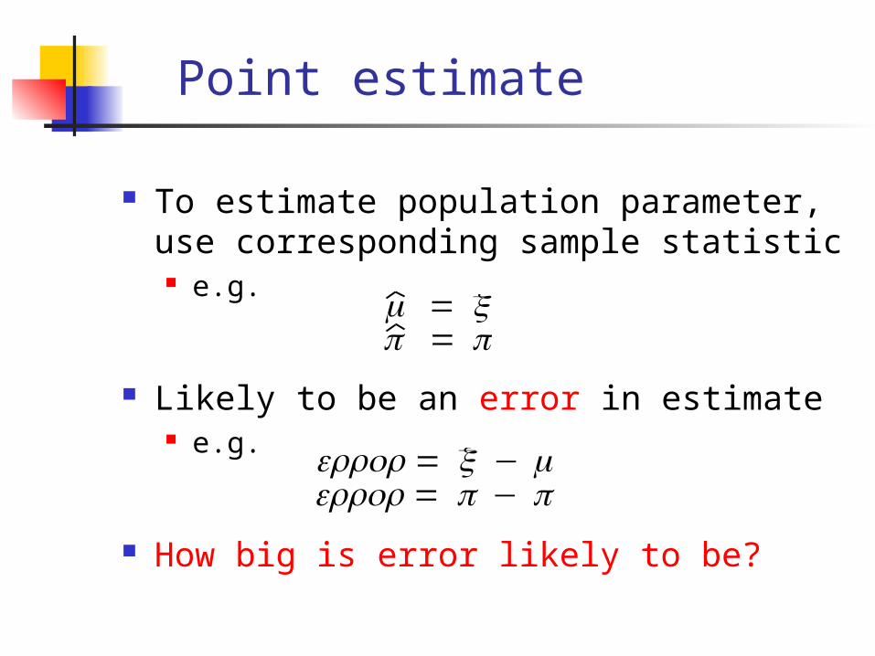
Point estimate

To estimate population parameter, use corresponding sample statistic e.g.

Likely to be an error in estimate e.g.

How big is error likely to be?

€

μ = x

€

π = p

€

error = x − μ

€

error = p − π

Error distribution

Error is random

Simulation from an ‘approx’ population could build up error distribution

Shows how large error from actual sample data is likely to be

Example

Silkworm survival after arsenic poisoning

How long will 1/4 survive? What is upper quartile?

Simulation

Approx population (same mean & sd as data)

Target = UQ from normal = 293.3 sec

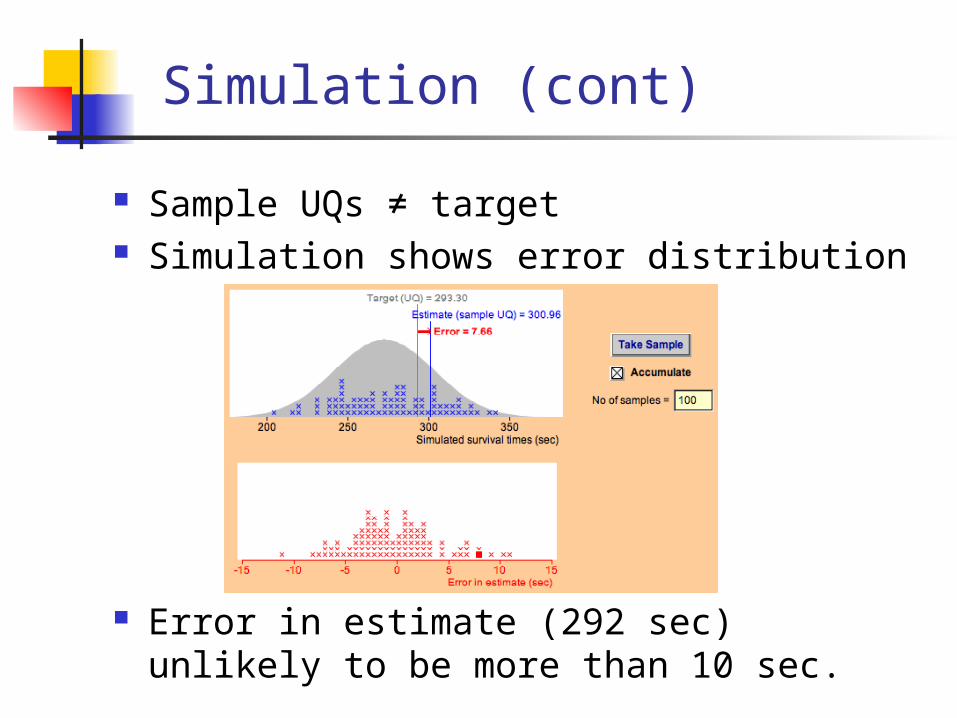
Simulation (cont)

Sample UQs ≠ target Simulation shows error distribution

Error in estimate (292 sec) unlikely to be more than 10 sec.

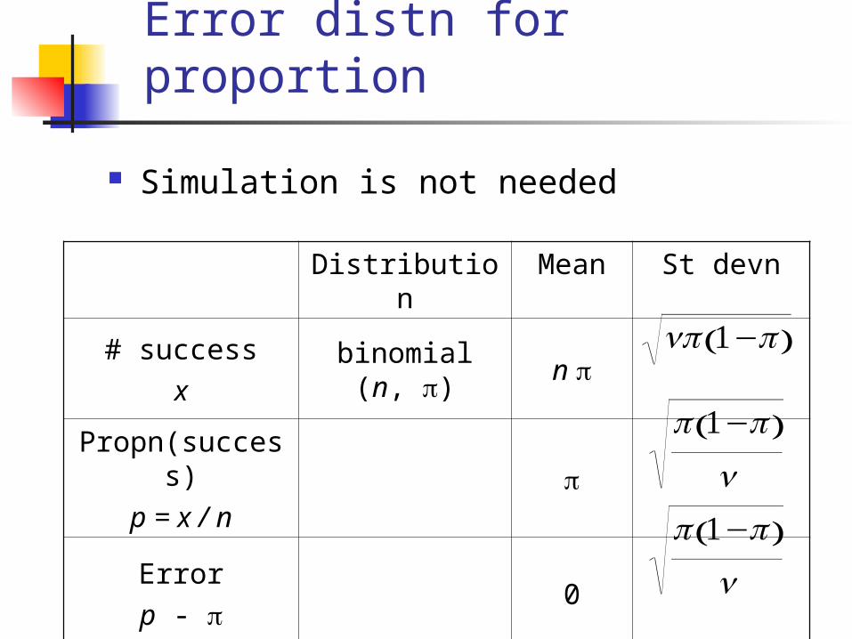
Error distn for proportion

Simulation is not needed

Distribution Mean St devn

# success

xbinomial (n, π) n π

Propn(success)

p = x / nπ

Error

p - π0

€

nπ 1−π( )

€

π 1−π( )n

€

π 1−π( )n

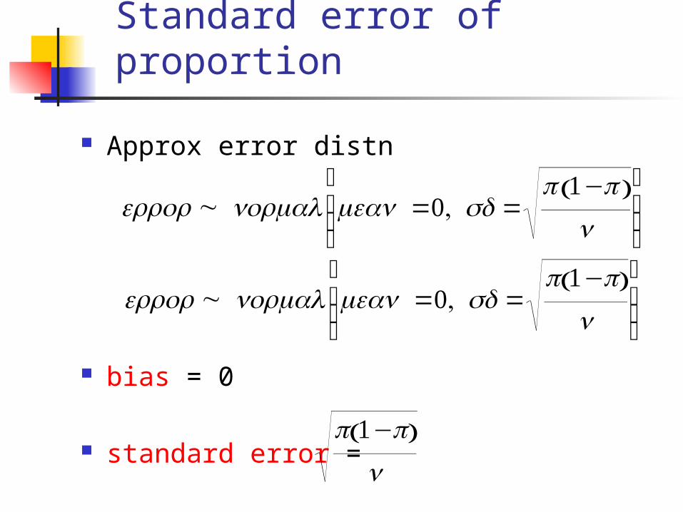
Standard error of proportion

Approx error distn

bias = 0

standard error =

€

error ~ normal mean=0, sd =π 1−π( )

n

⎛

⎝ ⎜ ⎜

⎞

⎠ ⎟ ⎟

€

p 1−p( )n

€

error ~ normal mean=0, sd =p 1−p( )

n

⎛

⎝ ⎜ ⎜

⎞

⎠ ⎟ ⎟

Teens and interracial dating

Point estimate:

Bias = 0

Standard error =

1997 USA Today/Gallup Poll of teenagers across country: 57% of the 497 teens who go out on dates say they’ve been out

with someone of another race or ethnic group.

€

π = p =  0.57

€

p 1−p( )n

= 0.57 1−0.57( )

497 = 0.022

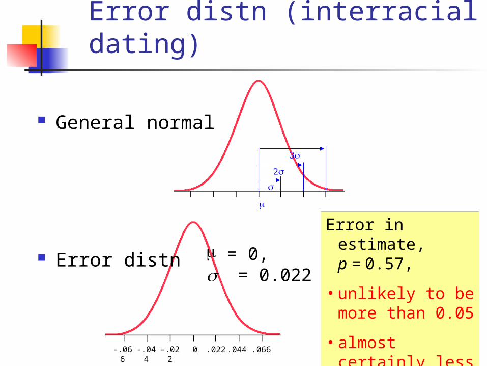
Error distn (interracial dating)

μ

2

μ = 0, = 0.022

0 .022 .044 .066-.022-.044-.066

General normal

Error distn

Error in estimate, p = 0.57,

• unlikely to be more than 0.05

• almost certainly less than 0.07

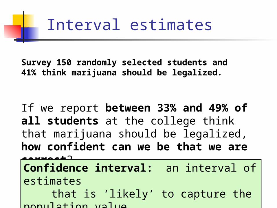
Interval estimates

Survey 150 randomly selected students and 41% think marijuana should be legalized.

If we report between 33% and 49% of all students at the college think that marijuana should be legalized, how confident can we be that we are correct?

Confidence interval: an interval of estimates that is ‘likely’ to capture the population value.

95% confidence interval

Legalise? p = 0.41, n = 150

70-95-100 rule of thumb Prob(error < 2 x 0.0412) is approx 95%

We are 95% confident that π is between0.41 – 0.0824 and 0.41 + 0.0824

0.33 and 0.49

€

error ~ normal0, p 1−p( )

n

⎛

⎝ ⎜ ⎜

⎞

⎠ ⎟ ⎟

= normal0, 0.0412( )

95% Conf Interval

Interpreting 95% C.I.

Confidence interval is function of sample data Random It may not include population parameter (π here)

In repeated samples, about 95% of CIs calculated as described will include π

We therefore say we are 95% confident that our single CI will include π

Teens and interracial dating

Point estimate:

Standard error =

95% C.I. is 0.57 - 0.044 to 0.57 + 0.044

0.526 to 0.614

1997 USA Today/Gallup Poll of teenagers across country: 57% of the 497 teens who go out on dates say they’ve been out

with someone of another race or ethnic group.

€

π = p =  0.57

€

p 1−p( )n

= 0.0222

We would prefer more decimals!

Teens and interracial dating

95% C.I. is 0.526 to 0.614

We do not know whether π is between 0.526 and 0.614

However 95% of CIs calculated in this way will work

We are therefore 95% confident that is in (0.526, 0.614)

St error & width of 95% C.I.

Smallest s.e. and C.I. width when: n is large p is close to 0 or 1

Biggest s.e. and C.I. width when: n is small p is close to 0.5

€

. . s e of propn= p 1−p( )

n

€

95% CI is p ± 2p 1−p( )

n

Margin of error

Public opinion polls usually estimate several popn proportions.

Each has its own “± 2 s.e.” describing accuracy

n = 350propn ± 2 x s.e.

Will vote for A 0.45 ± 0.0532

Will vote for X 0.04 ± 0.0209

Happy with govt 0.66 ± 0.0506

Wants tax cut 0.87 ± 0.0360

Margin of error (cont)

n = 350

Maximum possible is

propn ± 2 x s.e.

Will vote for A 0.45 ± 0.0532

Will vote for X 0.04 ± 0.0209

Happy with govt 0.66 ± 0.0506

Wants tax cut 0.87 ± 0.0360

€

±20.5 1−0.5( )

n = ± 1

n = ±0.055

“Margin of error” for poll

Requirements for C.I.

Sample should be randomly selected from population

“Large” sample size — at least 10 success and 10 failure (though some say only 5 needed)

If finite population, at least 10 times sample size

Case Study : Nicotine Patches vs Zyban

Study: New England Journal of Medicine 3/4/99)

893 participants randomly allocated to four treatment groups: placebo, nicotine patch only, Zyban only, and Zyban plus nicotine patch.

Participants blinded: all used a patch (nicotine or placebo) all took a pill (Zyban or placebo).

Treatments used for nine weeks.

Nicotine Patches vs Zyban (cont)

Conclusions:

Zyban is effective (no overlap of Zyban and not Zyban CIs)

Nicotine patch is not particularly effective(overlap of patch and no patch CIs)

Error distribution for mean

Again, a simulation is unnecessary to find the error distribution (approx)

Distribution Mean St devn

Sample meanApprox normal μ

ErrorApprox normal 0

€

x

€

x − μ

€

n

€

n

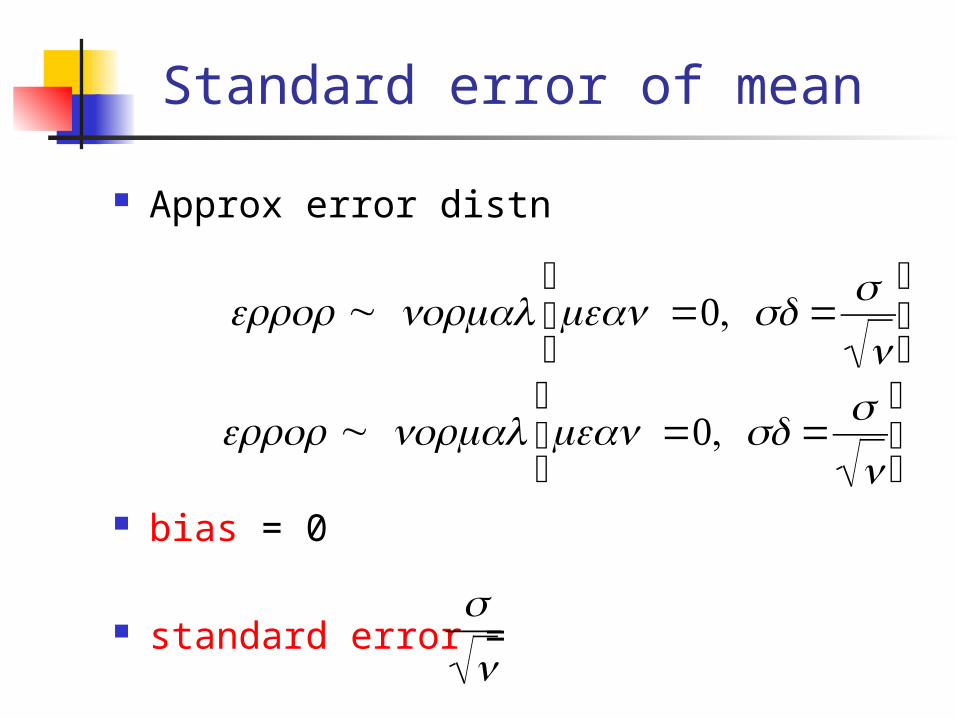
Standard error of mean

Approx error distn

bias = 0

standard error =

€

error ~ normal mean=0, sd=n

⎛

⎝ ⎜

⎞

⎠ ⎟

€

s

n

€

error ~ normal mean=0, sd=s

n

⎛

⎝ ⎜

⎞

⎠ ⎟

Poll: Class of 175 students. In a typical day, about how much time to you spend watching television?

Mean hours watching TV

n Mean Median StDev175 2.09 2.000 1.644

( ) 124.175

644.1.. ===

n

sxes

Point estimate:

Bias = 0

Standard error,

=  2.09 hours

€

μ = x

Standard devn & standard error

Sample standard deviation is approx stay similar if n increases

Standard error of mean is usually less than decreases as n increases

Don’t get mixed up between the two!

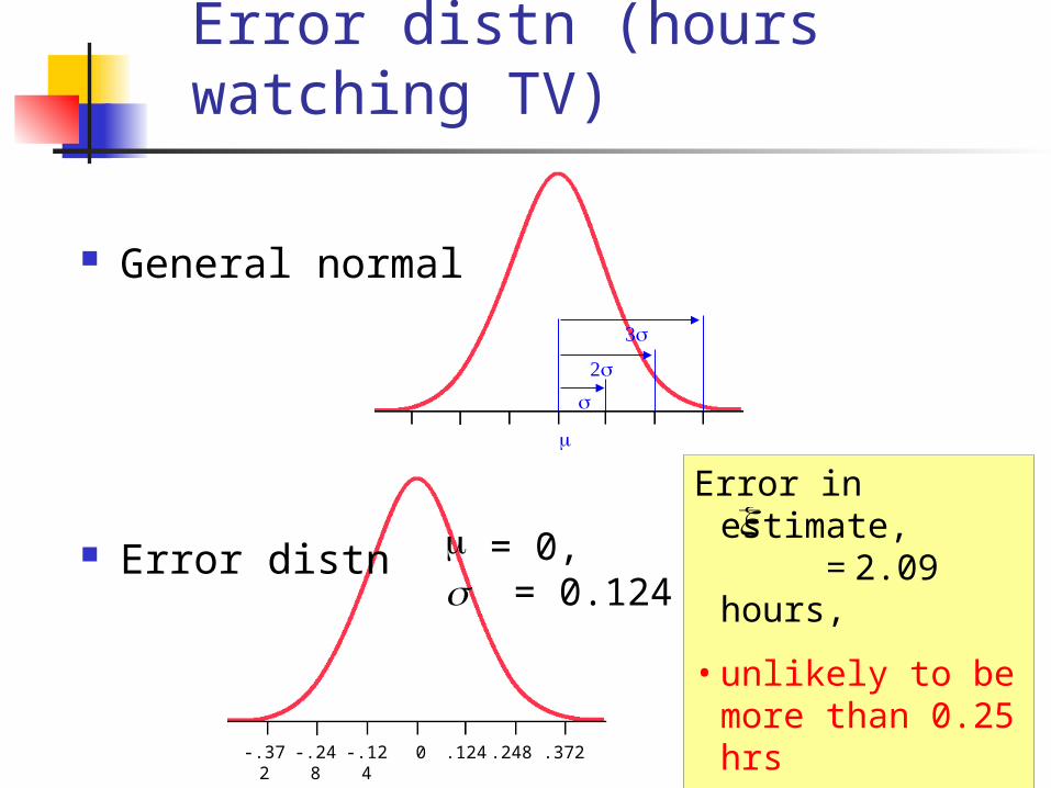
Error distn (hours watching TV)

μ

2

μ = 0, = 0.124

0 .124 .248 .372-.124-.248-.372

General normal

Error distn

Error in estimate,      = 2.09 hours,

• unlikely to be more than 0.25 hrs

• almost certainly less than 0.4 hrs

€

x

General form for 95% C.I.

0

se

2 se

se

Error distn

If error distn is normal zero bias & we can find s.e.

Prob( error is in ± 2 s.e.) is approx 0.95

95% confidence interval: estimate ± 2 s.e. 95% confidence interval: estimate ± 1.96 s.e.

(if really sure error distn is normal)

95% confidence interval

Mean hrs watching TV?    

70-95-100 rule of thumb Prob(error < 2 x 0.124) is approx 95%

We are 95% confident that μ is between2.09 – 0.248 and 2.09 + 0.248

1.84 and 2.34 hours

€

error ~ normal0, sn

⎛

⎝ ⎜

⎞

⎠ ⎟= normal0, 0.124( )

95% C. I.

€

x = 2.09 hrs, n = 175

Requirements for C.I.

Sample should be randomly selected from population

“Large” sample size  —  n > 30 is often recommended

If finite population, at least 10 times sample size

Problem with small n

Known  

Unknown

Variable width Less likely to include μ Confidence level less than 95%

€

x ± 1.96 n

works fine

€

x ± 1.96 sn

C.I. for mean, small n

Solution is to replace 1.96 (or 2) by a bigger number.

Look up t-tables with (n - 1) ‘degrees of freedom’

€

x ± tn−1 ×sn

Sample size, n d.f., n – 1 tn-1

100 99 1.98

30 29 2.05

10 9 2.26

5 4 2.78

Example: Mean Forearm Length

Data: From random sample of n = 9 men

25.5, 24.0, 26.5, 25.5, 28.0, 27.0, 23.0, 25.0, 25.0

95% C.I.: 25.5 2.31(.507) => 25.5 1.17 => 24.33 to 26.67 cm

€

x=25.5, s =1.52

s.e. x( ) =sn=1.52

9=.507

df = 8t8 = 2.31

What Students Sleep More?

Q: How many hours of sleep did you get last night, to the nearest half hour?

Notes: CI for Stat 10 is wider (smaller sample size) Two intervals do not overlap

Class n Mean StDev SE MeanStat 10 (stat literacy) 25 7.66 1.34 0.27Stat 13 (stat methods) 148 6.81 1.73 0.14

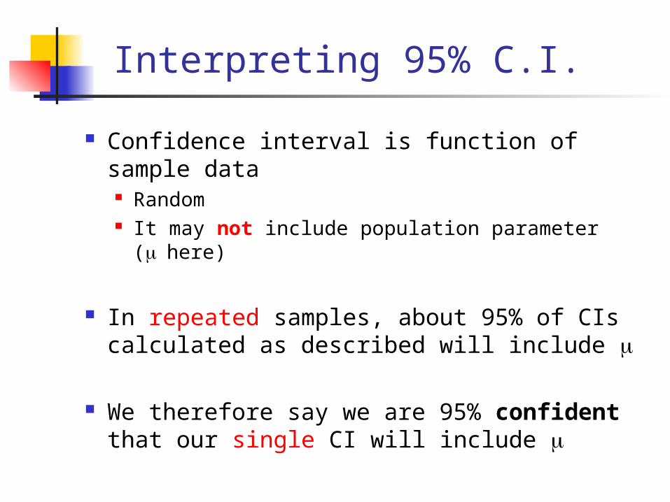
Interpreting 95% C.I.

Confidence interval is function of sample data Random It may not include population parameter (μ here)

In repeated samples, about 95% of CIs calculated as described will include μ

We therefore say we are 95% confident that our single CI will include μ