1

Objective

Compare the proportions of two independent means using two samples from each population.

Hypothesis Tests and Confidence Intervals of two proportions use the t-distribution

Section 9.3Inferences About Two Means

(Independent)

2

Definitions

Two samples are independent if the sample values selected from one population are not related to or somehow paired or matched with the sample values from the other population

Examples:

Flipping two coins (Independent)

Drawing two cards (not independent)

3

Notation

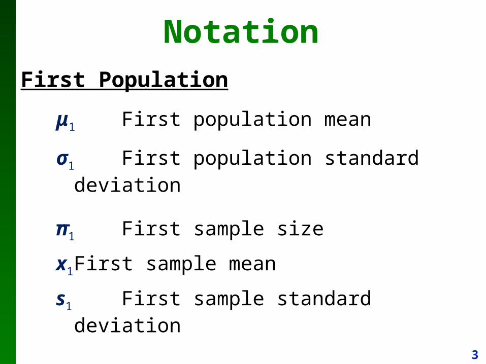
μ1 First population mean

σ1 First population standard deviation

n1 First sample size

x1First sample mean

s1 First sample standard deviation

First Population

4

Notation

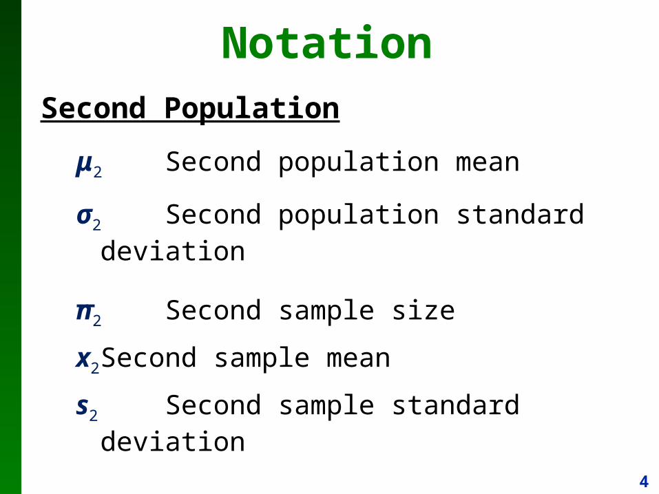
μ2 Second population mean

σ2 Second population standard deviation

n2 Second sample size

x2Second sample mean

s2 Second sample standard deviation

Second Population

5

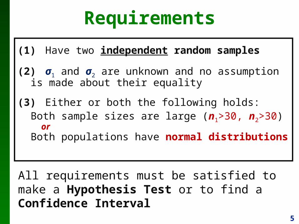
(1) Have two independent random samples

(2) σ1 and σ2 are unknown and no assumption is made about their equality

(3)Either or both the following holds:Both sample sizes are large (n1>30, n2>30) or

Both populations have normal distributions

Requirements

All requirements must be satisfied to make a Hypothesis Test or to find a Confidence Interval

6

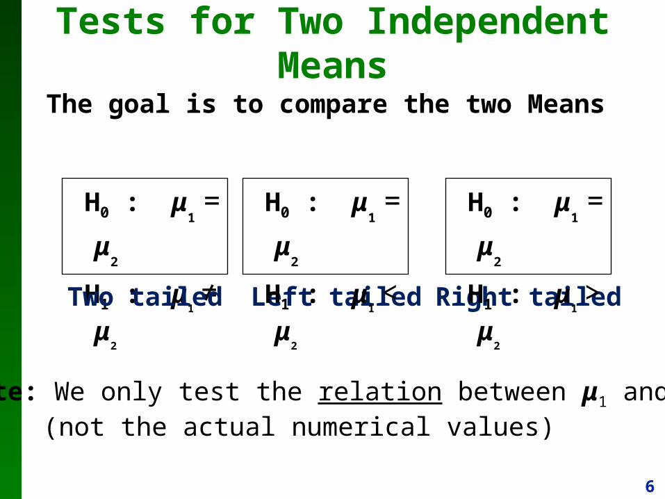
Tests for Two Independent Means

The goal is to compare the two Means

H0 : μ1 =

μ

2

H1 : μ1 ≠ μ

2

Two tailed Left tailed Right tailed

Note: We only test the relation between μ1 and μ2

(not the actual numerical values)

H0 : μ1 =

μ

2

H1 : μ1 < μ

2

H0 : μ1 =

μ

2

H1 : μ1 > μ

2

7

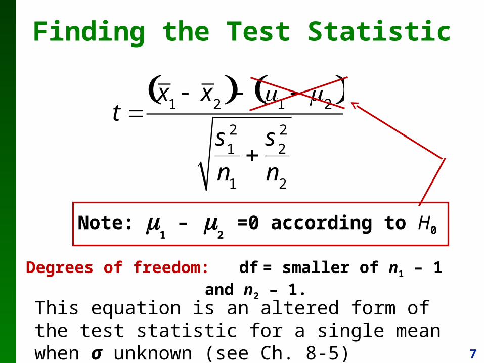
t x

1 x

2 1

2 s

12

n1

s

22

n2

Note: 1 –

2 =0 according to H0

Degrees of freedom: df = smaller of n1 – 1 and n2 – 1.

Finding the Test Statistic

This equation is an altered form of the test statistic for a single mean when σ unknown (see Ch. 8-5)

8

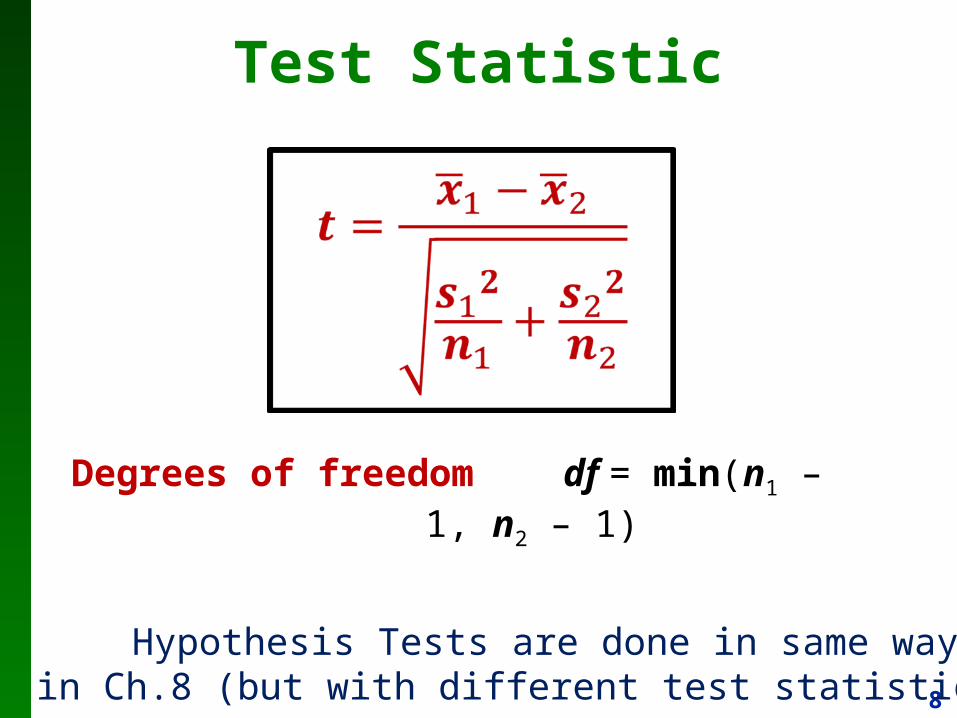
Test Statistic

Note: Hypothesis Tests are done in same way as in Ch.8 (but with different test statistics)

Degrees of freedom df = min(n1 – 1, n2 – 1)

9

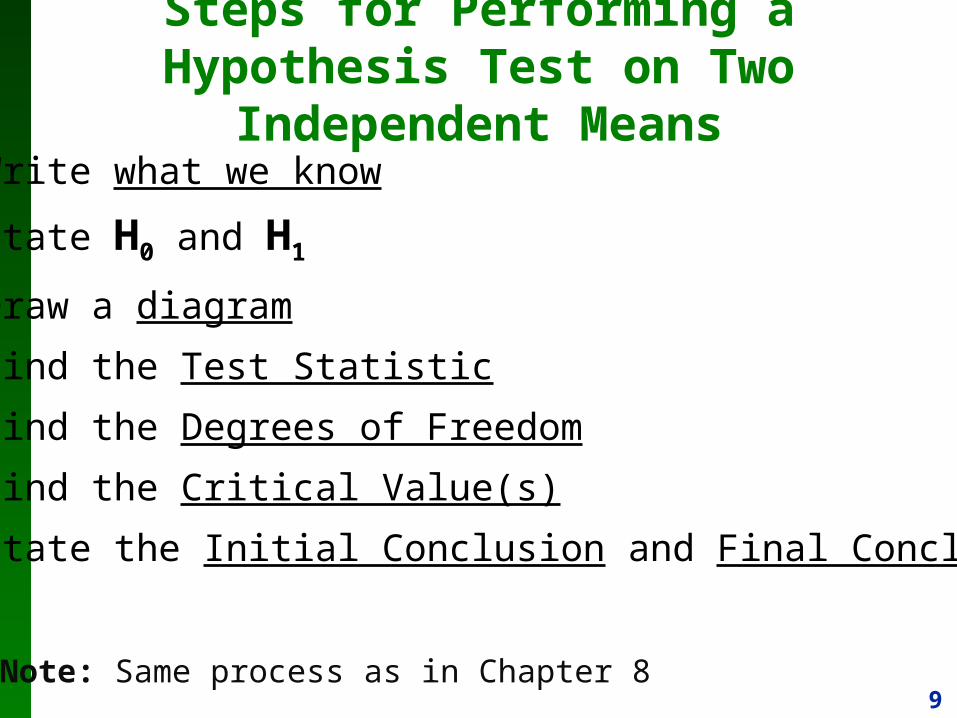
Steps for Performing a Hypothesis Test on Two Independent Means

• Write what we know

• State H0 and H1

• Draw a diagram

• Find the Test Statistic

• Find the Degrees of Freedom

• Find the Critical Value(s)

• State the Initial Conclusion and Final Conclusion

Note: Same process as in Chapter 8

10

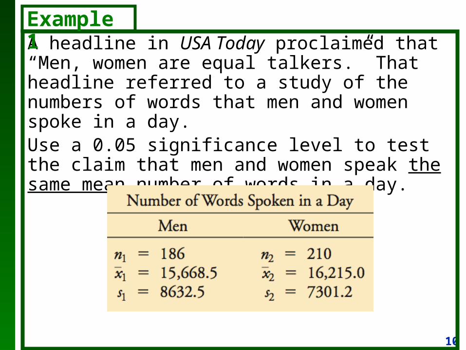
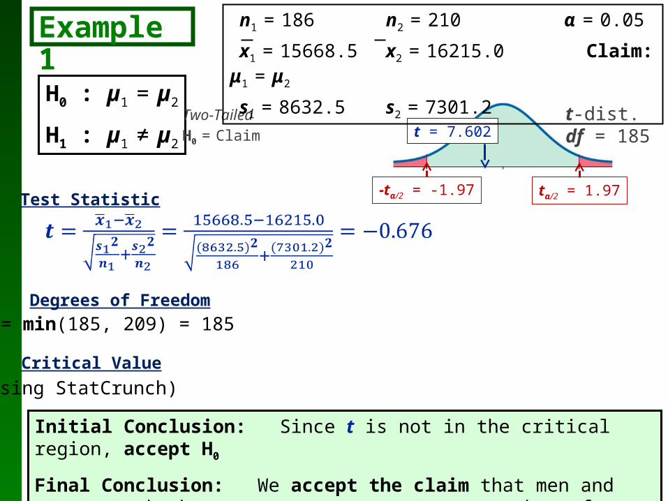
A headline in USA Today proclaimed that “Men, women are equal talkers.” That headline referred to a study of the numbers of words that men and women spoke in a day.Use a 0.05 significance level to test the claim that men and women speak the same mean number of words in a day.

Example 1

11

H0 : µ1 = µ2

H1 : µ1 ≠ µ2

Two-TailedH0 = Claim t = 7.602

tα/2 = 1.97

t-dist.df = 185

Test Statistic

Critical Value

Initial Conclusion: Since t is not in the critical region, accept H0

Final Conclusion: We accept the claim that men and women speak the same average number of words a day.

-tα/2 = -1.97

Example 1 n1 = 186 n2 = 210 α = 0.05

x1 = 15668.5 x2 = 16215.0 Claim: μ1 = μ2

s1 = 8632.5 s2 = 7301.2

Degrees of Freedom

df = min(n1 – 1, n2 – 1) = min(185, 209) = 185

tα/2 = t0.025 = 1.97 (Using StatCrunch)

12

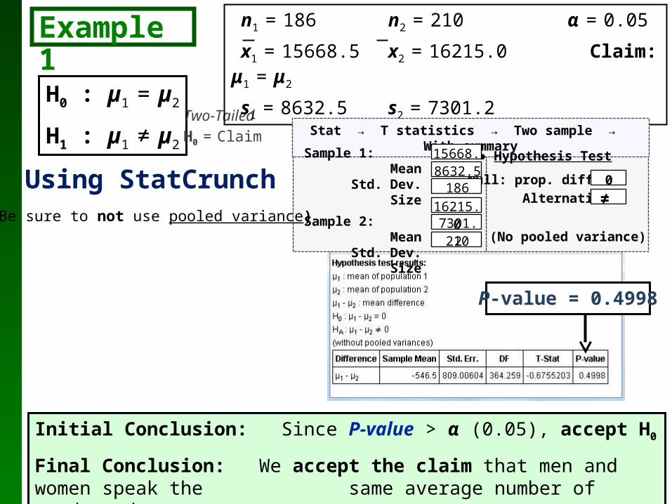
H0 : µ1 = µ2

H1 : µ1 ≠ µ2

Two-TailedH0 = Claim

Initial Conclusion: Since P-value > α (0.05), accept H0

Final Conclusion: We accept the claim that men and women speak the same average number of words a day.

Example 1 n1 = 186 n2 = 210 α = 0.05

x1 = 15668.5 x2 = 16215.0 Claim: μ1 = μ2

s1 = 8632.5 s2 = 7301.2

Stat → T statistics → Two sample → With summary

Null: prop. diff.=Alternative

Sample 1: MeanStd. Dev.

Size

Sample 2: MeanStd. Dev.

Size

● Hypothesis Test

P-value = 0.4998

15668.5

0

≠ Using StatCrunch 8632.5

18616215.07301.2

210 (No pooled variance)

(Be sure to not use pooled variance)

13

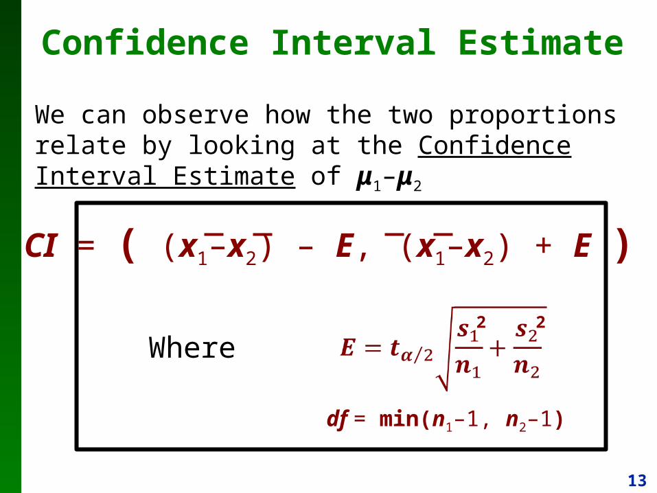
Confidence Interval Estimate

We can observe how the two proportions relate by looking at the Confidence Interval Estimate of μ1–μ2

CI = ( (x1–x2) – E, (x1–x2) + E )

Where

df = min(n1–1, n2–1)

2 2

14

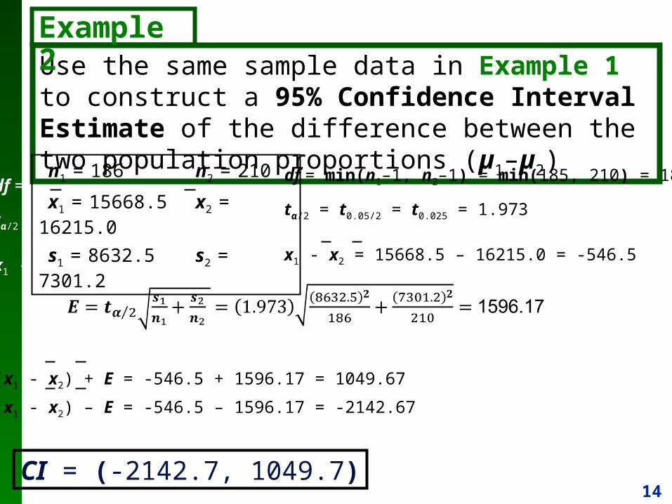
df = min(n1–1, n2–1) = min(185, 210) = 185

tα/2 = t0.1/2 = t0.05 = 1.973

x1 - x2 = 15668.5 – 16215.0 = -546.5

(x1 - x2) + E = -546.5 + 1596.17 = 1049.67

(x1 - x2) – E = -546.5 – 1596.17 = -2142.67

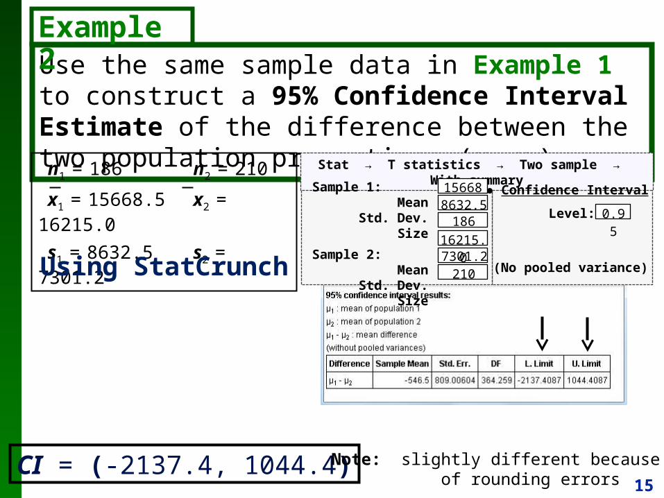
Use the same sample data in Example 1 to construct a 95% Confidence Interval Estimate of the difference between the two population proportions (µ1–µ2)

Example 2

n1 = 186 n2 = 210

x1 = 15668.5 x2 = 16215.0

s1 = 8632.5 s2 = 7301.2

df = min(n1–1, n2–1) = min(185, 210) = 185

tα/2 = t0.05/2 = t0.025 = 1.973

x1 - x2 = 15668.5 – 16215.0 = -546.5

CI = (-2142.7, 1049.7)

15

Use the same sample data in Example 1 to construct a 95% Confidence Interval Estimate of the difference between the two population proportions (µ1–µ2)

Example 2

CI = (-2137.4, 1044.4)

n1 = 186 n2 = 210

x1 = 15668.5 x2 = 16215.0

s1 = 8632.5 s2 = 7301.2

Stat → T statistics → Two sample → With summary

Level:

Sample 1: MeanStd. Dev.

Size

Sample 2: MeanStd. Dev.

Size

● Confidence Interval15668.5

0.95

Using StatCrunch

8632.5186

16215.07301.2

210

Note: slightly different because of rounding errors

(No pooled variance)

16

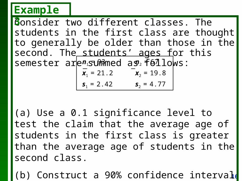
Consider two different classes. The students in the first class are thought to generally be older than those in the second. The students’ ages for this semester are summed as follows:

(a) Use a 0.1 significance level to test the claim that the average age of students in the first class is greater than the average age of students in the second class.

(b) Construct a 90% confidence interval estimate of the difference in average ages.

Example 3

n1 = 93 n2 = 67

x1 = 21.2 x2 = 19.8

s1 = 2.42 s2 = 4.77

17

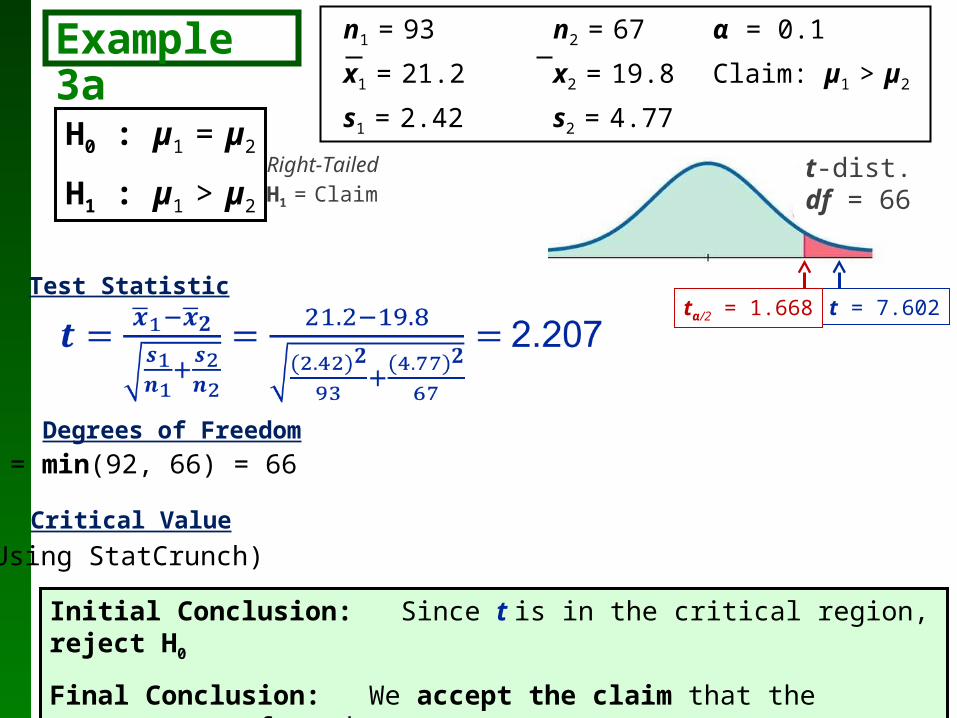
t = 7.602tα/2 = 1.668Test Statistic

Critical Value

Degrees of Freedom

df = min(n1 – 1, n2 – 1) = min(92, 66) = 66

tα/2 = t0.05 = 1.668 (Using StatCrunch)

H0 : µ1 = µ2

H1 : µ1 > µ2

Right-TailedH1 = Claim

n1 = 93 n2 = 67α = 0.1

x1 = 21.2 x2 = 19.8 Claim: µ1 > µ2

s1 = 2.42 s2 = 4.77

t-dist.df = 66

Example 3a

Initial Conclusion: Since t is in the critical region, reject H0

Final Conclusion: We accept the claim that the average age of students

in the first class is greater than that in the second.

18

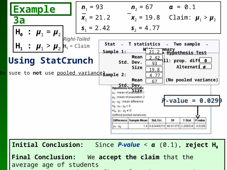
H0 : µ1 = µ2

H1 : µ1 > µ2

Right-TailedH1 = Claim

Example 3a n1 = 93 n2 = 67α = 0.1

x1 = 21.2 x2 = 19.8 Claim: µ1 > µ2

s1 = 2.42 s2 = 4.77

Stat → T statistics → Two sample → With summary

Null: prop. diff.=Alternative

Sample 1: MeanStd. Dev.

Size

Sample 2: MeanStd. Dev.

Size

● Hypothesis Test

P-value = 0.0299

21.2

0

≠

2.4293

19.84.7767 (No pooled variance)

Using StatCrunch(Be sure to not use pooled variance)

Initial Conclusion: Since P-value < α (0.1), reject H0

Final Conclusion: We accept the claim that the average age of students

in the first class is greater than that in the second.

19

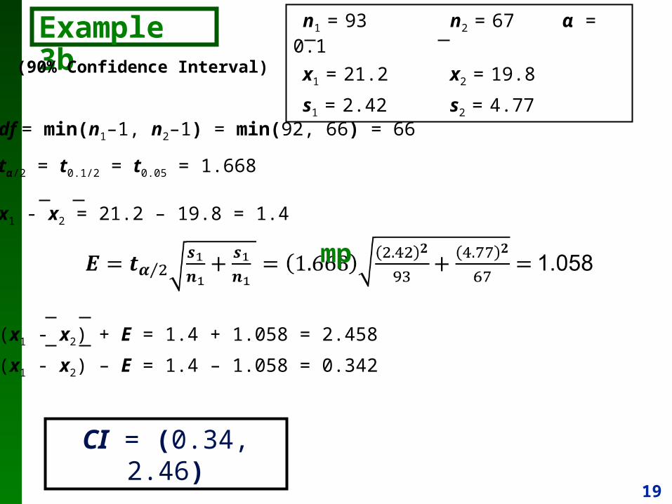
df = min(n1–1, n2–1) = min(92, 66) = 66

tα/2 = t0.1/2 = t0.05 = 1.668

x1 - x2 = 21.2 – 19.8 = 1.4

(x1 - x2) + E = 1.4 + 1.058 = 2.458

(x1 - x2) – E = 1.4 – 1.058 = 0.342

CI = (0.34, 2.46)

n1 = 93 n2 = 67α = 0.1

x1 = 21.2 x2 = 19.8

s1 = 2.42 s2 = 4.77

Example 3b

mp

(90% Confidence Interval)

20

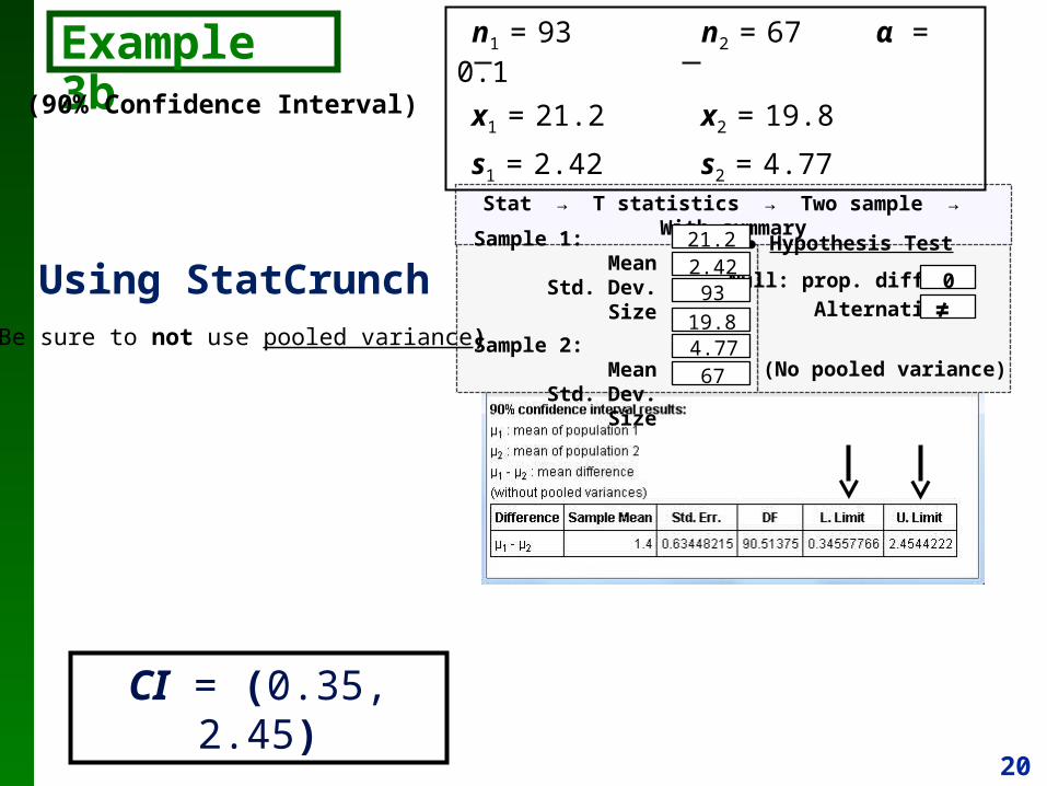
Example 3b

Stat → T statistics → Two sample → With summary

Null: prop. diff.=Alternative

Sample 1: MeanStd. Dev.

Size

Sample 2: MeanStd. Dev.

Size

● Hypothesis Test21.2

0

≠

2.4293

19.84.7767 (No pooled variance)

Using StatCrunch(Be sure to not use pooled variance)

CI = (0.35, 2.45)

n1 = 93 n2 = 67α = 0.1

x1 = 21.2 x2 = 19.8

s1 = 2.42 s2 = 4.77(90% Confidence Interval)