ESRI Geospatial Portal Technology - Esri - GIS Mapping Software

The University of Bergen, Norway
Nansen Environmental and Remote Sensing Center
Master Thesis
Web-GIS portal for multi-source oceanographic
data of Nordic Seas
By
Phalguni Pal Supervisor: Dhayalan Velauthapillai
Department of Informatics University of Bergen
May 2009

2 Web-GIS portal for multi-source oceanographic data of Nordic Seas
Preface This thesis titled 'Web-GIS portal for multi-source oceanographic data of Nordic Seas' is a web-based geographical information system (GIS), and is developed for partial fulfillment for Master Program in Informatics at the University of Bergen, Norway. The thesis was started in October 2008 and concluded in May 2009. This document provides a wide range of ideas to develop a web based marine and coastal management system. Due to large scale marine pollution by several causes, marine monitoring is essential to save the marine animals and keep the balance of the marine ecosystem. This thesis describes how to plan, design and implement a web based GIS. It also emphasizes about how to handle the spatial data in a very unique way, as spatial data have quite different structure than ordinary numerical or character data. This system displays various geographic positions of oceanographic stations with different parameters. To keep this report as ''Open'', all the confidential and related to industry internal documents have been taken out from this document. My enormous thanks go to my supervisor Dr. Dhayalan Velauthapillai. He was, in spite of difficulties, tremendously generous with his time and guidance and became a tremendous source of hope. I would like to thank Nansen Environmental and Remote Sensing Center (NERSC) for providing me such a nice thesis and for providing me a wonderful work environment. I am greatly indebted to my leader Dr. Torill Hamre (Scientist at NERSC) who helped me at every stage of my thesis work. Without her hearty co-operation this thesis would not possible to achieve. I also want to thank Dr. Alexander A. Korablev (Scientist at NERSC) who helped me by supplying oceanographic data for this thesis. And of course, I am thankful to my parents, brother and sister in law, who were encouraging and supporting me during the whole period I have been in Norway. The work with this thesis has given me a broader understanding of modern software development techniques, especially in the area of Web GIS Development. The work has been both challenging and satisfying, and I have gained knowledge within all studied theories. Phalguni Pal Bergen, Norway May, 2009

3 Web-GIS portal for multi-source oceanographic data of Nordic Seas
Table of Contents Preface ............................................................................................................................ 2 Table of Contents ............................................................................................................ 3 List of abbreviations ........................................................................................................ 5 Table of Figures .............................................................................................................. 7 List of tables .................................................................................................................... 8 Chapter 1 Introduction ................................................................................................... 9 1.1. Background .............................................................................................................. 9
1.1.1. What is GIS? ...................................................................................................... 9 1.1.2. Project source and initials .................................................................................. 9
DISPRO ................................................................................................................... 9 The Nordic Seas in the Global Climate System ..................................................... 12
1.2. Objectives of the thesis .......................................................................................... 13 1.3. Problem definition ................................................................................................... 14 1.4. Organization of the thesis ....................................................................................... 15 Chapter 2 Preparatory Studies .................................................................................... 16 2.1. Geography and activities of the study area ............................................................ 16 2.2. User of the project .................................................................................................. 17 2.3. Technology study ................................................................................................... 18
SAR ........................................................................................................................... 18 MapServer ................................................................................................................. 19
2.4. Background of geographic data of this thesis ......................................................... 20 The three different databases for initial data to climatology ....................................... 24
Chapter 3 Development Methods ................................................................................ 28 3.1. Available Technology and Methodologies .............................................................. 28 3.2. Object Oriented Software Development ................................................................. 30 3.3. Development Method ............................................................................................. 31 Chapter 4 Database Design, Source and Technology ................................................ 37 4.1. Software and tools for this Thesis .......................................................................... 37 4.2. Database Selection ................................................................................................ 37 4.3. Data source ............................................................................................................ 40 4.4. Database design .................................................................................................... 43

4 Web-GIS portal for multi-source oceanographic data of Nordic Seas
4.5. MapServer Installation ............................................................................................ 48 4.6. Database connectivity ............................................................................................ 51 Chapter 5 GUI Description .......................................................................................... 52 5.1. The existing DISPRO ............................................................................................. 52 5.2. New modifications in DISPRO ................................................................................ 55 5.3. Working with GUI ................................................................................................... 59 5.4. Result ..................................................................................................................... 61 Chapter 6 Discussions and Challenges ....................................................................... 62 6.1. Discussion .............................................................................................................. 62
An oceanographic Database (ODB) .......................................................................... 62 Spatially Enabled Database ....................................................................................... 63 Problems in Linux Platform ........................................................................................ 63 The remaining part of GUI ......................................................................................... 66
6.2. Challenges ............................................................................................................. 69 Chapter 7 Conclusion .................................................................................................. 71 References .................................................................................................................... 72 Appendix 1 .................................................................................................................... 74 Appendix 2 .................................................................................................................... 77

5 Web-GIS portal for multi-source oceanographic data of Nordic Seas
List of abbreviations ASAR Advance Synthetic Aperture Radar CGI Common Gateway Interface DISMAR Data Integration System foe Marine Pollution and Water Quality DISPRO DISMAR Prototype ESRI Environmental Systems Research Institute EPPL Environmental Planning and Programming Language GeoTIFF Geographical Tagged Image File Format GIS Geographic Information System GUI Graphical User Interface HIRLAM High Resolution Limited Area Model HTML Hyper Text Markup Language NERSC Nansen Environmental and Remote Sensing Center NORHAB Norwegian Harmful Algal Bloom Services NS Nordic Seas MODIS Moderate Resolution Imaging Spectroradiometer MERIS MEdium Resolution Imaging Spectrometer NIVA Norwegian Institute of Water Research OGC Open GIS Consortium OVF Open Virtualization Format ODB Oceanographic Database SAR Synthetic Aperture Radar

6 Web-GIS portal for multi-source oceanographic data of Nordic Seas
SRS Spatial Reference System SSH Sea Surface Height SST Sea Surface Temperature TIFF Tagged Image File Format TOPAZ Towards an Operation Prediction system for the North Atlantic European coastal Zones WMS Web Map Service WFS Web Feature Service XML eXtensible Markup Language

7 Web-GIS portal for multi-source oceanographic data of Nordic Seas
Table of Figures Fig 1: Pictorial overview of DISMAR Project . .............................................................. 10
Fig 2: Pictorial view of data flow in the InterRisk (DISPRO). ....................................... ..11
Fig 3(i): The stations where data were collected ........................................................... 13
Fig 3(ii): Pictorial view of the objectives of this thesis .................................................... 14 Fig 4: Map of Norwegian Sea and Arctic sea. ............................................................... 16
Fig 5: NS database content 1900-2006: by Source . ..................................................... 22
Fig 6.Quality-duplicate controlled, merged initial database. .......................................... 24
Fig 7: Objectively analyzed databases for requested grid net ....................................... 25
Fig 8: Mean and anomalies fields at standard levels, in layers and on density ............. 25
Fig 9: Waterfall Model for Software Development ........................................................ 29
Fig 10: Pictorial representation of Relational Unified Process ....................................... 32
Fig 11: ‘Cost of Change’ curve with the waterfall model ............................................... 33
Fig 12: Cost of changes graph with time using light weight process ............................. 34
Fig 13: MySQL GIS Data types (abstract types in gray) ............................................... 40
Fig 14: Station position in Profiling floats (total station: 2908) ....................................... 41
Fig 15: Station position in Research Vessels (total station: 2404) ................................. 42
Fig 16: Database relationship of ODB ........................................................................... 43
Fig 17: cities table with three rows ................................................................................ 44
Fig 18: border2 table with SHAPE2 geometry type (polygon) column ........................... 45
Fig 19: geometry_columns table (metadata type) ......................................................... 45
Fig 20: spatial_ref_sys (metadata type) ........................................................................ 46
Fig 21: The over all pictorial view of spatially enabled database ................................... 47
Fig 22: The reply from localhost ‘http://127.0.0.1’ .......................................................... 49
Fig 23: Pictorial view of Software environment .............................................................. 50
Fig 24: Graphical user Interface of existing DISPRO system ........................................ 52
Fig 25: All layers of DISPRO’s NORHAB GUI ............................................................... 53
Fig 26: The pictorial view of old DISPRO ...................................................................... 54
Fig 27: New system view ............................................................................................... 57
Fig 28: The new architecture of Web GIS DISPRO ....................................................... 58
Fig 29: HTML request generating form .......................................................................... 59

8 Web-GIS portal for multi-source oceanographic data of Nordic Seas
Fig 30: a piece of HTML code pointing to MapServer ................................................... 60
Fig 31: Positions of the cities on the map ...................................................................... 60
Fig 32: Loading data in the database through query ..................................................... 63
Fig 33: connection.ovf file .............................................................................................. 64
Fig 34(i): Reply from ogrinfo command before driver installation for MySQL ................ 65
Fig 34 (ii): Reply from ‘ogrinfo –formats’ command after driver installation for .............. 65
Fig 35: Station temperature-depth profile ...................................................................... 68
Fig 36: Station graph of salinity for a large area of Nordic Sea ..................................... 68
List of tables Table1: NS database content country wise ................................................................... 23
Table2: NS database content: reference period for anomalies computing .................... 24
Table3: Workflow of the database and climatology compilation .................................... 27
Table4: Comparison among deferent databases .......................................................... 38
Table5: The hardware requirement for MS4W .............................................................. 48
Table6: Difference between DISPRO 3 [21] and Web GIS DISPRO ............................. 56

9 Web-GIS portal for multi-source oceanographic data of Nordic Seas
Chapter 1 Introduction
1.1. Background
During the last three decades, a powerful technology called Geographic Information System (GIS) has silently altered the way people view and live. Most people are unconscious using of GIS in their daily life. People use GIS in almost every where in their day to day life from morning to night directly or indirectly. Few example of using GIS are in mobile phone, navigator, air traffic control, weather forecast news, TV and radio etc.
1.1.1. What is GIS? A geographic information system (GIS) or geographical information system is a computer system for capturing, storing, checking, integrating, manipulating, analyzing and displaying data related to positions on the Earth's surface. GIS technology can be used for scientific investigation, resource management, environmental impact assessment, asset management, cartography, archaeology, geographic history, marketing, urban planning, criminology, logistic, Prospective Mapping and many other purpose. For example, using satellite images GIS could easily predict emergency response times in the occasion of a natural-disaster, or GIS can be use by a company to place a new location to make improvement of an earlier under-served market.
1.1.2. Project source and initials This master thesis is based on two projects running at Nansen Center called “DISPRO” and “The Nordic Seas in the Global Climate System” [16]. Here in below the two projects are discussed briefly.
DISPRO
DISPRO is the web GIS prototype resulting form of the DISMAR project [19]. The overall objective of DISMAR was to develop a modern intelligent information system for monitoring and forecasting marine environment to improved management of pollution crises in coastal and ocean regions of Europe, in support to public administrations and

10 Web-GIS portal for multi-source oceanographic data of Nordic Seas
emergency services responsible for prevention, mitigation and recovery of crises such as oil spill pollution and harmful algal blooms (HAB). InterRisk is a follow-up project where we besides developing DISPRO further also work on a number of other issues, such as other web-GIS systems, new data delivery services, processing services, chaining of services, ontology, and a generic portal for environmental services with web-GIS viewer etc. InterRisk addresses the need for better access to information for risk management in Europe, both in cases of natural calamity and industrial mishaps. The overall objective is to develop an advance system for interoperable GMES (Global Monitoring for Environment and Security) monitoring and forecasting services for environmental management in marine and coastal areas. The InterRisk project will consist of an open system architecture based on established GIS and web services protocols, and the InterRisk services to be applied for several European regional seas. The two projects (DISMAR and InterRisk) have similar goals, but InterRisk has expanded the range of services and functionalities available, utilizing the latest advances in both ICT theory and technologies/tools [26]. On the later stage DISPRO has been improved as part of the InterRisk project [20] in a master thesis by Oleksandr Kit [21].
Fig 1: Pictorial overview of DISMAR Project [19].
The InterRisk pilot system and services will be validated by users responsible for crisis management in case of oil spills, harmful algal blooms and other marine pollution events, in Norwegian, UK/Irish, French, German, Polish and Italian coastal waters.
Pollution event in recent years, such as the Prestige oil tanker wreckage (oil spills) polluting huge areas in the coastal zone of Spain and neighbouring countries, as well as the Server accident on January 2007 outside Fedje island polluting nearly coastline and
11 Web-GIS portal for multi-source oceanographic data of Nordic Seas
damaging sea birds, sea animals and sea fishes. For Norwegian waters, with big fish farming industry, monitoring and forecasting of harmful algal blooms (HABs) are equally important as toxic HABs and oil spills can cause significant economic loss for the European aquaculture industry. As a tool to monitor oil spills and harmful algal blooms, the Nansen Center together with other partners in a European research project developed a web-base GIS called DISPRO. This system has later been enhanced in several projects and is currently running at Nansen Center. DISPRO is based on W3C[22], OGC[23] and ISO[24] standard and uses a public domain tool UMN Mapserver [28] to process and deliver geographic data in standard raster formats for display in a web browser. It allows the multiple data provides to upload data in the servers that deliver data to DISPRO portal. This portal runs in a common browser, allowing end users to access all data without having to install expansive or machine demanding GIS tools. All processing is done by the data nodes and the DISPRO portal.
Fig 2: Pictorial view of data flow in the InterRisk (DISPRO) [20].

12 Web-GIS portal for multi-source oceanographic data of Nordic Seas
The Nordic Seas in the Global Climate System This project was funded by the associaction called INTAS(the International Association for the promotion of co-operation with scientists from the New Independent States of the former Soviet Union)[18]. INTAS was eastablished in 1993 by the European Community and like-minded countries as an international non-profit association under Belgian law. The member countries of this associasion are of two types and called INTAS-members and EECA-partner countries respectively. Most of the European countries are counted as INTAS-members and all countries of former USSR are counded as EECA-partner countries. The main objectives of INTAS is to promote scientific research activities in the NIS (New Independent States) and scientific co-operation between scientists in these countries and the international scientific communities. INTAS’ objectives were achieved mainly by financing collaborative projects, working in networks, supporting innovative works etc. The association also has provided scientific insfrastructure and lots of felloships to the young scientiscs from EECA countries. INTAS corganizes scientific conferences, summer schools and many trining evens for the scientists. INTAS projects and activities covered both fundamental and applied research, in all fields of exact, natural, social and human sciences. Oceanographic data with different parameters like salinity, temperature, pH and dissolved oxygen in water etc and others details information about the different sea locations are collected from different stations of Nordic Seas (Norwegian, Greenland, Iceland and Barents Seas). Scientists at Nansen Centers in Bergen and St. Petersburg have created an oceanographic database (ODB) system containing an extensive amount of collected and analyzed data. The oceanographic data were collected from many different marine research institutes and from many similar projects. The details about oceanographic data source will be discussed in the next chapter. The ODB system has three different databases, one is of initial data with chance of duplicity, second is of observed and interpolated data and last one is of objective analyzed monthly fields data with errors estimates. The duplicates identification algorithms allow automatic detection and metadata/profiles merging to generate complete oceanographic station composition from multiple duplicates. Applied quality control algorithms were intended to preserve the regional variability and to produce a dataset which further can be used for computing of climatology fields with high spatial resolution.

13 Web-GIS portal for multi-source oceanographic data of Nordic Seas
Fig 3(i): The stations where data were collected [25]
1.2. Objectives of the thesis The prime objective of this thesis is to develop a web-based application to display all different parameters in the ODB system in a browser as a station graph, section graph or section map. By clicking on certain station of the map the system will display all the characteristic of oceanographic parameters without using any other software. The system will also be able to ingest other data sources, such as satellite images and forecasts from numerical models, and display these data on the same map as the ODB data. The system will be developed using W3C (World Wide Web Consortium) and OGC (Open Geospatial Consortium) standards for web-based GIS (Geographic Information Systems). The other objective is to add more features to an existing web-mapping system called DISPRO. The Figure 3(ii) shows a pictorial over view of existing web-mapping DISPRO and what this thesis will add to old DISPRO to make it an improved web based GIS system.

14 Web-GIS portal for multi-source oceanographic data of Nordic Seas
Fig 3(ii): Pictorial view of the objectives of this thesis
1.3. Problem definition This thesis is developed as a separate part of an existing web-base GIS called DISPRO [9]. As mentioned, the aim of the thesis is to add some totally new features to the old DISPRO system. The problem definition for this thesis is as follows: i) To add and merge new features without disturbing the current working existing system. ii) The new formatted system has to be capable to deal with all types of geographic data (in-situ data, vector data, raster data, remote sending data etc) without any limitation. iii) To create an oceanographic database (ODB) which can access the system in a suitable and well organized way. iv) To create an effective and user friendly system.

15 Web-GIS portal for multi-source oceanographic data of Nordic Seas
v) To create a system which is independent on the use of any desktop GIS tool purchasable in the market like ArcIMS, ArcExplorer, ArcMap, MapFish, MapBeder etc. A system which is dependent only on open-source existing software (UMN Mapserver, cocoon web-publishing framework, MSCross etc) to avoid re-implementation and should work with an ordinary PC and a common web browser. vi) To create a system which is capable of displaying section graph, section map, depth series and time series for a particular oceanographic station.
1.4. Organization of the thesis This thesis document is organized in to seven chapters. Chapter 1 contains general introduction about the thesis, a short description of project source and objectives of the thesis. Chapter 2 starts by having a brief discussion of action area and describes the initial background studies for required data and technologies. The chapter 3 says about available technologies and software development methodologies which are used for system design. The database design and the details of software/tools installation has been discussed in the chapter 4. Following, in the chapter 5, a detailed description about graphical user interface (GUI) of web based GIS system is given. The very next chapter 6 describes about the developer’s achievements in the process of making the system, the current status of the system and the unavoidable challenges during the software process. The last chapter 7 draws the conclusion with showing the way for further enhancement and future works.

16 Web-GIS portal for multi-source oceanographic data of Nordic Seas
Chapter 2 Preparatory Studies
Initially, developer had to do some related preliminary studies to understand the theme of the thesis. Thus to give a broader perspective a brief preparatory study is discussed in this chapter.
2.1. Geography and activities of the study area
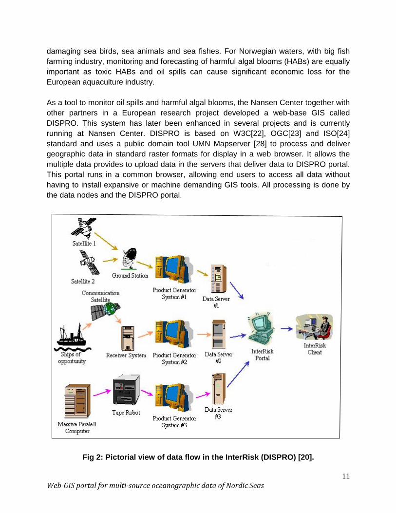
The Norwegian Sea, the Greenland Sea and the Icelandic Sea are usually as a group called as the Nordic Sea.
Fig 4: Map of Norwegian Sea and Arctic sea.
17 Web-GIS portal for multi-source oceanographic data of Nordic Seas
The Norwegian Sea is part of the North Atlantic Ocean, northwest of Norway, located between the North Sea and the Greenland Sea. It nearby the Iceland Sea to west and the Barents Sea to the Northwest, it is split from the Atlantic Ocean by a submarine edge running between Iceland and the Faroe Island. To the Northe, Jan Mayen Ridge separated from Greenland Sea. The average depth of Norwegian Sea comprises 1600-1750 meters, its area is equal to 1.38 million sq. km and the greatest depth is 3,970 meters. The Greenland Sea is the northernmost part of the North Atlantic Ocean nearby south of the Arctic Ocean. It encompasses some 1.20 million sq. km. The average depth of the Greenland Sea is close to 1,450 meters. The deepest recorded point of 5600 meter
has been found at Molloy Deep, in the Fram Strait between north-eastern Greenland and Svalbard.
2.2. User of the project As stated before this is an EU project. After studying about the present trend of economical investments in Nordic Seas developments and according to several project reports (DISMAR, InterRisk, GMES), the developer could say that the following groups of users will utilize this Web-GIS based marine monitoring and management system in practice. [21]
• Regional and national environmental and disaster response agencies, navies
• Ice breaker fleet and port authorities
• Scientific community
• Consulting services up to a smaller degree
• National authorities (fisheries, environmental management)
• Fish industries
• Aquaculture Industries
• The general public

18 Web-GIS portal for multi-source oceanographic data of Nordic Seas
2.3. Technology study Successful implementation of the planned web-based GIS project on the Nordic Sea would be impossible without deeply technology study. The main technologies used for the system are SAR –imagery and Web-GIS techniques. These techniques are going to be discussed here in below:
SAR It’s very important to know that what the SAR is and how does it help GIS? Synthetic Aperture Radar (SAR) is an active microwave tool in operational oceanography, producing high-resolution imagery of the Earth's surface in all weather. The SAR is an active device, i.e. it creates its own light of the scene to be viewed, like a camera with flash. The satellite's light is coherent, i.e. all the light in any flash is exactly in phase, like a laser, so it does not simply scatter over the distance between the satellite and the Earth's surface. A SAR instrument can measure both intensity and phase of the reflected light, resulting not only in a high sensitivity of the surface, but also in some three-dimensional capabilities. [27] SAR systems are ideal for investigating oceanic processes because of their high resolution and operation independent of weather and time of day. That’s why SAR is use for remote sensing of oil spilt, vessel surveillance and sea ice studies. A number of unexpected features of SAR imagery of oceanographic interest have been observed in flights of SAR systems in the past decade, including the artifacts of bathymetry1
1 Bathymetry is the study of underwater depth.
, currents, waves, and winds. These interpretations can depend on subtle connections of, e.g., the current, with the small-scale surface waves which are sensed by the SAR at intermediate incidence angles. The theory of SAR-usages for remote sensing is very easy to understand. The sensor mounted in satellite or airplane sends out a radar wave called backscatter. Particularly imaging radar (RAdio Detection and Ranging) is used for this purpose. Imaging radar is similar to flash camera which provides its own light to clarify an area on the ground and take a picture at radio wavelengths. It uses an antenna and computer tapes to record images. This type of radar shows the lights that are reflected back towards the radar antenna. Surface roughness is very impotent input for radar backscatter model. Sea surface oil spilt and algal increase the amount of viscosity, which reduces backscatter

19 Web-GIS portal for multi-source oceanographic data of Nordic Seas
and produces much darker imagery. Various other parameters can also produce darker imagery; therefore the oil detection in the prepared form requires use of other technologies and high operational skills. [12]
MapServer The user wanted to develop a web-GIS system based on existing open source tools(UMN MapServer, cocoon web-publishing framework, MSCross etc) for monitoring oil spilt and harmful algal blooms of Nordic seas. User also wanted to access web-based GIS system via Internet from any point in the world (in most cases, an ordinary PC with a common Web-browser is sufficient) and might enable its users to get information about the oceanographic data from various places in the world. The majority of data for marine research and management of Nordic Seas are raster or other gridded data. The DISMAR (2005a) report propose to select open source OGC WMS (Web Maps Service)/ WFS (Web Feature Service) open-source MapServer of University of Minnesota as the base system for development of Web-based GIS application.
MapServer is an open source geographic data reproduction device written in C language. Mapserver originally developed in the mid-1990’s at the University of Minnesota ForNet project in cooperation with NASA, and the Minnesota Department of Natural Resources (MNDNR). MapServer is now further developed and maintained by OSGeo (The Open Source Geospatial Foundation) [28]. MapServer is capable of handling vector data, in-situ data, remote sensing data, enabling both raster and vector data to be displayed on the same map, in a projection selected by user. MapServer handles a series of formats for raster and vector data, as well as spatially enabled databases. Some more feature of MapServer is as below [28]:
• Support for popular scripting languages and development environments
o Python, PHP, Perl, Ruby, Java, and .NET framework
• Operating System (platform) support
o Linux, Windows, Mac OS X, Solaris etc.
• Support of numerous Open Geospatial Consortium (OGC) standards
o WMS (client/server), non-transactional WFS (client/server), WMC, WCS,
Filter Encoding and more

20 Web-GIS portal for multi-source oceanographic data of Nordic Seas
• A multitude of raster and vector data formats
o TIFF/GeoTIFF, EPPL7, and many others via GDAL (Geospatial Data
Abstraction Library).
• Data base support
o ESRI Shapefiles, Oracle Spatial, MySQL, DB2, MS SQL Server(with ESRI
ArcSDE), PostgreSQL( withPostGIS) and many others via OGR
• Map projection support
o On-the-fly map projection with 1000s of projections through the Proj.4
library (a library for projecting map data)
Mapserver is a CGI program and needs to install on a Web Server. Its installation and properly working depend on the type of the system platform, additional databases and associate modules etc.
2.4. Background of geographic data of this thesis At the beginning of the INTAS-4620 project, detail analysis of oceanographic data sources for Nordic Seas region was carried out. [13] Especially after 1990 necessary amount of oceanographic data was not on hand and were scattered among different organizations and projects but many of them were not moved to any centralize database. It was noticed that large observational programs did not take place for the south and north of the NS. The all collected data by deferent organization and projects were of different format. It was hard task to merge all different formatted data into a common dataset. In this regards few steps for data transformation were impose like quality/ duplicate controls, merging, interpolation at the standard level and objective analysis etc. Initial data collection process was started from Arctic and Antarctic Institute (AARI). A large number of dataset were requested from different data centers, marine institute and field projects. Nearly 2.5 million stations were combined. Special database was developed for the data storage and data processing. It’s includes numerous converters from data formats to common database format (Interbase 7.0). The metadata are stored in two database tables ‘Station’ (14 fields) and ‘Station_info’ (9 fields) linked by the unique key. Required fields for first table include coordinate, date, time and station version. Remaining fields represent station quality flag, station source name, vessel name, country name, bottom depth and depth of last measured level. Last three

21 Web-GIS portal for multi-source oceanographic data of Nordic Seas
columns are bottom depth from bathymetry at the station, minimum, maximum depth in five kilometres radius around the station. The second table contains supplementary information including ‘station’ international country/vessel codes, cruise number, station number in the cruise, instrument type, name of the secondary source etc. Data from each initial source were transferred into separate initial database with full composition of available parameters. Finally the geographic area for NS region in the INTAS-4620 project was reduce to the area 60º N-82ºN, 40ºW- 70ºE. Before merging all data, databases passed the preliminary quality control (QC). The merging procedure and integrated database structure were design to simplify subsequent duplicate control and to eliminate low accuracy data. The strategy was to not store all available stations which have already stored in the initial database but produce an operational database with complete metadata and reduce instrumental and partiality spatial. Two additional tables ‘Duplicate’ and ‘Duplicate_info’ were introduced into the database similar to ‘Station’ and ‘Staion_Info’ table’s but with two additional fields. These two extra fields were ‘ID number from source database’ and ‘access index’. These fields provide a connection to source databases and information about station status during merging process with duplicate control. At first, only the metadata from all initial databases were merge into 12 monthly databases. Stations were taken by low accuracy instruments and with less than three observed levels were skipped. At this stage the total number of stations were reduce from approximately 2.5 million to 1 million. [16] The ‘Duplicates problem’ is common in oceanography and is difficult to resolve particularly for huge datasets and numerous initial sources. To solve this problem, a specific hierarchy was introduced (‘exact’, ‘full’, ‘TSO2’, and ‘interpolated variants’). When all stations metadata and profiles coincide each other and which is easy to find out is called ‘exact’ duplicates. The ‘full’ duplicates means that some metadata fields at stations can be different and distributed among the multiple stations. The ‘TSO2’ duplicates are defined if salinity, temperature and oxygen profiles at stations are the same while metadata and other profiles may be different. The last ‘interpolated variant’ assumes that stations suspected to be duplicates are interpolated variants of the same profiles. To check it the variables for one profile are linearly interpolated on levels of another profile. The practical algorithm of duplicates identification was started from the first station in a merged datasets. At the beginning the database includes just metadata from all initial databases by means of empty variables (profiles) tables. After automatic and expert control with metadata and profiles merging the total number of stations left in the integrated database appears to a little bit more than 400,000.

22 Web-GIS portal for multi-source oceanographic data of Nordic Seas
The number of station distribution by sources in the final database is illustrated in Fig 3. Totally 26 different sources made a contribution, eight of them supplied more than 10,000 stations each. This project received more than 150,000 stations from ‘The Climatic atlas of the Arctic Seas’ (Mathishov et al., 2004), 80,000 from WOD01 (Stephens et al., 2002), and about 35,000 from the ‘Institute of Marine Research’ (Bergen, Norway). Around 64% of stations were obtained by two countries: Russia (> 132,000) and Norway (> 123,000). About more than 68,000 stations included from unknown origin. The big number of stations with missing country names and vessel names implies that even algorithm designed to improve the metadata content can’t restore substantial parts of information. The figure below will demonstrate the number distribution by the source in the merged database for Nordic Sea.
Fig 5: NS database content 1900-2006: by Source [25]. The section graph above shows the different source projects and numbers of obtained stations from a particular project. The X-axis represent the ‘YEARS’ (1900 - 2006) and Y-axis represents ‘Number of Stations by source’. It is clear from the graph that the ODB got most number of data during the time 1957 to 1992. More than 15,000 data
1900 1910 1920 1930 1940 1950 1960 1970 1980 1990 2000 2010YEARS
0
1000
2000
3000
4000
5000
6000
7000
8000
9000
10000
11000
12000
13000
14000
15000
16000
Num
ber o
f sta
tions
by
sour
ce
source->stationsODB_CA [154488]WOD2001 [83830]IMR9002 [34730]AARIod [27634]OBNINSK [27614]ODB_ICES [16727]VEINS_H [14919]MIKE2006 [11123]AARI_TGM [7375]WOD2005 [7233]AARIcr [5215]NPICD [3100]Cearex [2825]NNDCD [2416]ARGO [2414]PNSEC [756]AWI_CD [731]MMBI [386]TRACTOR [313]OVERFLOW [304]ESOP [215]GSP [181]MAIA [150]VEINS [113]NANSEN [10]CriuseReport [6]
23 Web-GIS portal for multi-source oceanographic data of Nordic Seas
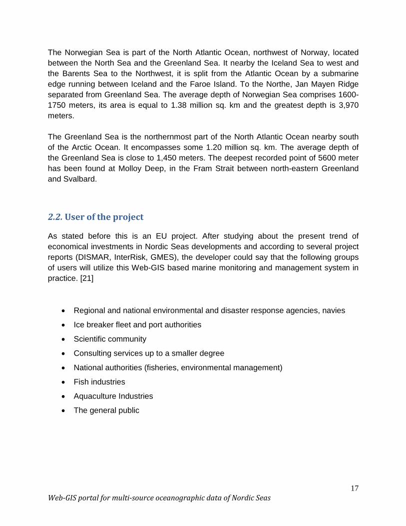
were collected during the year 1984, 1989 and 1990. The ODB_CA source project (green colour) supplied the maximum number of data (> 150,000). The tables 1 below shows the total numbers of data were collected from different countries of Europe, Asia and Canada. More than 68,000 data were composed into ODB from unknown source. The names of the countries are placed in the table according to the decreasing number of total data were found. More than 60% of ODB were received only from two countries like Russia and Norway and then the next largest number of data source is from unknown origin.
Sl. No.
Country Stations #
1 USSR/RUSSIA 132,081 2 NORWAY 123,740 3 UNKNOWN 68,678 4 UNITED KINDOM 20,408 5 ICELAND 19,808 6 UNITED STATES 15,946 7 GERMANY 11,157 8 DENMARK 5,125 9 POLAND 2,268 10 JAPAN 1,560 11 NETHERLAND 1,416 12 CANADA 1,203
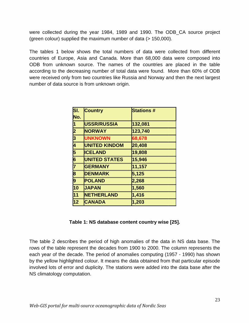
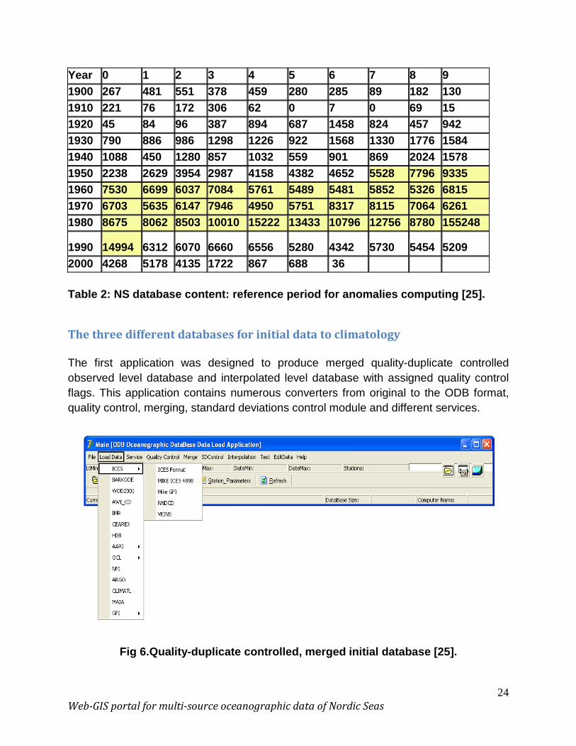
Table 1: NS database content country wise [25]. The table 2 describes the period of high anomalies of the data in NS data base. The rows of the table represent the decades from 1900 to 2000. The column represents the each year of the decade. The period of anomalies computing (1957 - 1990) has shown by the yellow highlighted colour. It means the data obtained from that particular episode involved lots of error and duplicity. The stations were added into the data base after the NS climatology computation.
24 Web-GIS portal for multi-source oceanographic data of Nordic Seas
Year 0 1 2 3 4 5 6 7 8 9 1900 267 481 551 378 459 280 285 89 182 130 1910 221 76 172 306 62 0 7 0 69 15 1920 45 84 96 387 894 687 1458 824 457 942 1930 790 886 986 1298 1226 922 1568 1330 1776 1584 1940 1088 450 1280 857 1032 559 901 869 2024 1578 1950 2238 2629 3954 2987 4158 4382 4652 5528 7796 9335 1960 7530 6699 6037 7084 5761 5489 5481 5852 5326 6815 1970 6703 5635 6147 7946 4950 5751 8317 8115 7064 6261 1980 8675 8062 8503 10010 15222 13433 10796 12756 8780 155248
1990 14994 6312 6070 6660 6556 5280 4342 5730 5454 5209 2000 4268 5178 4135 1722 867 688 36 Table 2: NS database content: reference period for anomalies computing [25].
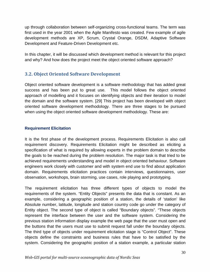
The three different databases for initial data to climatology The first application was designed to produce merged quality-duplicate controlled observed level database and interpolated level database with assigned quality control flags. This application contains numerous converters from original to the ODB format, quality control, merging, standard deviations control module and different services.
Fig 6.Quality-duplicate controlled, merged initial database [25].

25 Web-GIS portal for multi-source oceanographic data of Nordic Seas
The second comprises of graphical user interface and provide access to the data and tools for visualization and analysis. Embedded objective analysis module allows computing of the gridded fields. This application makes available modules for data selection, filtering, storing, editing, export, import, objective analysis and visualization.
Fig 7: Objectively analyzed databases for requested grid net [25] The last application provides access to objectively analyzed fields and service for further processing and visualization. This application allows mean field computing from objective analysis monthly fields, anomaly fields and climatological comparison.
Fig 8: Mean and anomalies fields at standard levels, in layers and on density surfaces [25]

26 Web-GIS portal for multi-source oceanographic data of Nordic Seas
Technological procedure
STEP I
Compilation of the source database
Definition of the metadata comparison and data structure
Developing of converters from original data format to the initial Interbase 7.0 format
Download data from initial data source into individual data bases
Metadata update by adding bottom up depths from girded bathymetry and last measured level
at station
Removal of the stations out side the NS geographic origin
Quality control and setting the quality control flags on observed level data
STEP II
Compilation of the integrated observed level database, duplicate control, assigning quality control flag
Merging of the individual database into integrated database with instrument control
Automatic duplicate control with metadata and profiles merging
Standard deviation (SD) control in the layer around the standard levels, quality control flags
assigning on values outside the previous SD

27 Web-GIS portal for multi-source oceanographic data of Nordic Seas
STEP III Compilation of the standard level database, assigning quality control flags
Vertical interpolation on the standard level with accepting quality flags, compilation of the
standard level database
Standard deviation (SD) control at the standard level, quality control flags assigning
values at pervious level SD
STEP IV Compilation of the objectively analyzed database, computing climatological means
Objective analysis of the monthly fields at the standard level on 0.25º X 0.5º latitude /longitude
grid
Download OA field data into database
Computing climatological mean and anomalies
Table 3: Workflow of the database and climatology compilation for the Nordic Seas [16].

28 Web-GIS portal for multi-source oceanographic data of Nordic Seas
Chapter 3 Development Methods
3.1. Available Technology and Methodologies Software development process could be compared with a car making process. The automobile company cautiously understands the demands of market and makes plan for a new model. The following is the starting point in the making of a car. First lists of requirements like total number of seats, interior space, external height, length, power of engine, colour etc are decided by the company. The car designer and automobile engineer are appointed to make the design and engine respectively. Both of them analyse the requirements and draw some figures. After passing through some improvements and putting new ideas, the plan for making process is finalized and then created. Development of software follows more or less the same steps as those needed to make a car. Software development has five major phases; they are requirement, analysis, design, implementation and testing. Every software development process should pass over through these essential phases. Now there is a big question that what are the benefits of following any software development method? A software development process is a structure required on the development of a software product. Any software development project is aimed to achieve some goal objective. Software development method helps to achieve the goal and to finish the project successfully. Various software processes tell the developer about different steps to follow and it also say about requirement understanding, system modelling and system building steps. Development methodologies act as director during the software system implementation which is also at some point depends on used technology. Now it will be attempted to explain, why object oriented software development procedure or modern software development methods should follow instead of old procedural development methods. Up to last decade waterfall development method was the most popular method for software development and it still in used in some extent. It has observed that customers often don’t know or are unable to communicate what they really want. Customers change their minds as they learn more or as a consequence of changes in market and technology. Waterfall model is not suitable in requirement changing environment. Some drawbacks of waterfall model are as follows:
• Document driven model which customer cannot understand properly. Customers get just a textual specification of software architecture.

29 Web-GIS portal for multi-source oceanographic data of Nordic Seas
• First time client observe a working product which sometimes does not meet the requirements and reconstructing is costly and time consuming.
• Works best when developers know that what they are doing i.e. requirements are stable and is well-known.
• The waterfall model simplifies task scheduling, because there are no iterative or overlapping steps. It does not allow for much revision.
Fig 9: Waterfall Model for Software Development [33]
So software developers needed some method which was iterative, evolutionary and suitable for a changeable environment. The agile software development methodologies grew up in the mid-1990s as part of a response against "changeable situation". The Agile software development is a group of software development methodologies based on iterative development with similar principles, where requirements and solutions build
30 Web-GIS portal for multi-source oceanographic data of Nordic Seas
up through collaboration between self-organizing cross-functional teams. The term was first used in the year 2001 when the Agile Manifesto was created. Few example of agile development methods are XP, Scrum, Crystal Orange, DSDM, Adaptive Software Development and Feature-Driven Development etc. In this chapter, it will be discussed which development method is relevant for this project and why? And how does the project meet the object oriented software approach?
3.2. Object Oriented Software Development Object oriented software development is a software methodology that has added great success and has been put to great use. This model follows the object oriented approach of modelling and it focuses on identifying objects and their iteration to model the domain and the software system. [29] This project has been developed with object oriented software development methodology. There are three stages to be pursued when using the object oriented software development methodology. These are: Requirement Elicitation It is the first phase of the development process. Requirements Elicitation is also call requirement discovery. Requirements Elicitation might be described as eliciting a specification of what is required by allowing experts in the problem domain to describe the goals to be reached during the problem resolution. The major task is that tried to be achieved requirements understanding and model in object oriented behaviour. Software engineers work closely with customer and with system end use to find about application domain. Requirements elicitation practices contain interviews, questionnaires, user observation, workshops, brain storming, use cases, role playing and prototyping. The requirement elicitation has three different types of objects to model the requirements of the system. “Entity Objects” presents the data that is constant. As an example, considering a geographic position of a station, the details of ‘station’ like Absolute number, latitude, longitude and station country code go under the category of Entity object. The second type of object is called “Boundary objects”. “These objects represent the interface between the user and the software system. Considering the previous station information display example the web page that the user must open and the buttons that the users must use to submit request fall under the boundary objects. The third type of objects under requirement elicitation stage is “Control Object”. These objects define the constraints and business rules that have to be satisfied by the system. Considering the geographic position of a station example, a particular station
31 Web-GIS portal for multi-source oceanographic data of Nordic Seas
should not display duplicate data or information. This type of duplicate control (constraint) falls under the control object. Requirement analysis Requirements Analysis is the process of understanding the customer needs and expectations for the system or application. Requirements describe how a system should act or a description of system properties or attributes. The requirements are further analyses and elaborated at this phase. Activity diagram and sequence diagram are two such mythologies for standard documentation. The result of this phase of the development process is to understand requirements clearly and proper documentation of the requirements. System design In the object oriented software development concept, the system design process stage defines object interface, collaboration and arranges the foundation for the development. The system design explains the details of the architecture, components, modules and interfaces. System development The system development stage is the stage where the design is coded or implemented to make working software that fulfils user requirements. System development includes coding and testing at various level of process.
3.3. Development Method Relational Unified Process There are few popular software development methods currently available in software industry. They are IBM’s Relational Unified Process (RUP) and Agile software development methods (XP, Scrum, DSDM etc.) The unified process is an extensible framework which describes the various activities that must be followed in the progress period of software. It defines key points that are characteristic and that should be kept in mind through out the software development process. The RUP defines four phases in the whole “Project lifecycle”. These are inception, elaboration, construction and transition. Iterations moves throughout the phases.

32 Web-GIS portal for multi-source oceanographic data of Nordic Seas
Fig 10: Pictorial representation of Relational Unified Process [30] . Agile development methods (eXtreme Programming-XP) The cost of changing during the software development process has an exponential increasing behaviour with time period. One reason that increases change of cost behaviour is the usage of heavy weight software development processes. The inflexible and time consuming procedures and the need to keep the newly added related documents make for most of making changes. [36]

33 Web-GIS portal for multi-source oceanographic data of Nordic Seas
Fig 11: ‘Cost of Change’ curve with the waterfall model [34]
To get over from increasing weight of the processes, a group of seventeen software experts met in 2001to discuss key principal of Agile development. The came up with the following manifesto that says “We are uncovering better ways of developing software by doing it and helping others do It”. [35] Extreme programming (XP) is one of the most known and popular agile methods. But Scrum and Lean are also getting popularity rapidly. XP is based on a set of independent Practices, Principles and Values. The XP emphasises on four great values which are Communication, Simplicity, Feedback and Courage. There should be regular, open minded and high level of communication between the developer and customer. Simplicity means keep the things easy and simple. That is keeping the software design simple. The customer should be development team member and would provide continuous feedback after getting each piece of working software. Courage tells that to go ahead without fear of get stuck.

34 Web-GIS portal for multi-source oceanographic data of Nordic Seas
Carefully using the compilation of selected practices and tools, the cost of late changing factor could be decrease like the graph below:
Fig 12: Cost of changes graph with time using light weight process
During developing this thesis the key practices of XP method has carefully been implemented. In this section all those practices which have great impact on this thesis will be discussed step by step. The Planning Game: The planning game is the division of responsibility between business (customer) and development (developer). The business people consider the features and decide how important it is, and the developers fix the cost to implement that features. [37] The planning game was carefully implemented at beginning of this thesis. The time plan, initial exploration, release plan, iteration plan etc were done at the start point of this thesis with the customer. On-site Customer/ Customer Team Member An XP project strongly recommends that the customer or a representative of the customer should be a member of development team. The customer will empower to determine requirements, set priorities, and answer questions of developers. This thesis has been developed sitting at customer’s site and with many close and kin co-operations.
35 Web-GIS portal for multi-source oceanographic data of Nordic Seas
Test Driven Development (TDD) XP tells first write test before coding. Developers have to write a failing unit test before to write a production code. The first test must fail without any production code. The TDD was very hard to implement in this thesis but it has been tried to do this. There was no definite testing tool available for testing map script in this thesis. So, test was not run before production code frequently. But test was made before any small release. User stories The user stories are the primary definitions of the user requirements. The user stories are short summarized description of what the user wants the system should do. User stories are not descriptive like use cases. It acts as reminder of the conversation the developer has made with the customer. The numbered user stories help developer for planning purpose or planning game. The stories for this thesis were:
i) Data from the oceanographic database (ODB) must be imported in a spatially enabled database that can be accessed by MapServer. The system must be able to import station data, interpolated fields and climatological fields (mean and anomalies). The administrator must be able to select which of the available parameters and fields he/she wants to import.
ii) The spatially enabled database must be made available in the DISPRO system. New data inserted must become visible immediately. The user typically selects a subset of the database, by specifying a geographic area and time range of interest.
iii) The system must keep track of available remote sensing, in situ and model forecast data in the Nordic Seas. Users must be able to select data of interest and display it on the map.
iv) DISPRO will display a symbol for each station on the map. When clicking on a station symbol, the system will display a list of measured parameters at the chosen station. From this list, the user can select one or more parameters and the system will generate a station graph.

36 Web-GIS portal for multi-source oceanographic data of Nordic Seas
Acceptance Tests Customer will accept the piece of working software by running acceptance test. If the software pass the test then customer will receive it, otherwise customer will ask again to fix the error. In this thesis customer did exactly as stated above before it was accepted. Simple Design An XP project should be the simplest program that meets the user requirements. There is no need to build much for the future but focus should be on providing business values. Developers should keep simplified design which is easy to implement. In this thesis the design has made simple for easy execution. Pair Programming XP programmers write all production code in pairs, two programmers works together at a machine. Pair programming has been shown by many experiments to produce better software at lower cost than programmers work alone. It is very important practice of XP. This thesis has been developed by a single developer with close communication of customer. So pair programming was not possible in this case.

37 Web-GIS portal for multi-source oceanographic data of Nordic Seas
Chapter 4 Database Design, Source and Technology
4.1. Software and tools for this Thesis In this section software and tools used for the thesis will be discussed. As mentioned earlier, customers have some restriction on the required software and tools for thesis. Developer had to use only available open source software and tools which fits well with the existing DISPRO system. After discussion with the customer, developer comes to the decision to go with the following software and tools: Platform / OS: Linux or Windows (XP/ Vista) [Linux is 1st priority for NERSC. Windows was suggested to make development easier ] Database Language: MySQL Script Language: HTML, XML, Java Script, Ajax, python Programming Language: Java, MapScript (UMN MapServer) Application Server: Apache Tomcat Web-Development Framework Cocoon GIS tool: UMN MapServer (MS4W), GDAL/OGR [43] It will be explained why these software and tool has been selected here in below:
4.2. Database Selection It was crucial to choose the database for oceanographic data. Since the amount of data in the North Sea Database is very large (3GB) and eventually customer would like to have all of it accessible from web-GIS, it was important that the database selected is powerful, fast and flexible. It was also very important to select a database which was supported by UMN MapServer which is used by the existing DISPRO. It is very vital to mention here that Mapserver does not support all database languages.

38 Web-GIS portal for multi-source oceanographic data of Nordic Seas
After searching many sources in Internet and especially Mapserver website [28] the developer got the information that MapServer supports a number of databases. These are as below: i) Oracle (Oracle Corporation) ii) MySQL (Sun Microsystems) iii) DB2 (IBM). iv) Microsoft SQL Server (with ESRI ArcSDE or MapInfo Professional). v) PostgreSQL( Postgre SQL Global Development Group ) and few more. It has been seen that PostgreSQL with PostGIS supports are very frequently used in many other GIS projects. A comparative study of all above mentioned databases are shown here in below:
DB Name
Max DB Size
Max table size
Max row size
Max columns Per row
Max Blob/Clob Size
Max CHAR Size
Max Number size
Min date value
Max date value
DB2
512TB
512 TB
32,677B
1012
2GB
32 KB
64 bits
0001
9999
MS SQL server
524,258 TB
524,258 TB
Unlimited
30000
2GB
2 GB
126
0001
9999
MySQL
Unlimited
2GB -16TB
64 KB
4096
4GB
64KB (text)
64 bits
1000
9999
Oracle
Unlimited
4GB
Unlimited
1000
Unlimited
4000B
126 bits
-4712
9999
Postgre SQL
Unlimited
32TB
1.6TB
250 – 1600 depending on type
1GB
1GB
Unlimited
-4713
>9999
Table 4: Comparison among deferent databases [7] The above table shows the capability of various databases supported by MapServer. Since this thesis had to tackle huge amount of data and MySQL 5 supports unlimited database size. It’s also fit in Linux and Windows platform. MySQL has all the features which were required for this thesis. Nansen Center (customer) had the licence version of MySQL 5 and was installed in Johansen Linux server (johansen.nersc.no). So it was decided to select MySQL to make an oceanographic database (ODB) for this thesis.

39 Web-GIS portal for multi-source oceanographic data of Nordic Seas
The ODB development was started with normal MySQL tables but after several attempts it did not work properly. So developer had to choose spatially enable MySQL to make ODB. MySQL has the capability to handle spatial or geometry data (for example oceanographic data). Here is very important to know that what is spatially enabled MySQL and why it is used? A spatial database is a database that can analyze to generate, store and query data related to objects in space or surface, including points, lines and polygons. A typical or ordinary database understands different numeric, character and string types of data. A typical database does not recognize geographical data. So database should have some additional quality to know the spatial data. This database functionality is called geometric features. [40] The open Geospatial Consortium (OGC) [23] created the simple features specification which is of OpenGIS standard and it can store geographical data like lines, points, muli-points, line-string, polygons etc. Simple features are based on two dimension geometry and supports both spatial and non-spatial attributes. MySQL has all above mentioned features of OGC and OpenGIS standards. The spatial functionality was first introduced in MySQL in the version 4.1. MySQL use WKT (Well Known Text) / WKB (Well Known Binary) format to create geometry values. Both are use for representing vector geometry. MySQL provides a number of functions that take as input parameters a Well-Known Text representation and, optionally, a spatial reference system identifier (SRID). They return the corresponding geometry. WKT accepts GeomFormText() and WKB accepts GeomFromWKB() of any geometry type as its first argument. An implementation also provides type-specific construction functions for construction of geometry values of each geometry type. [41] The figure in below is the MySQL data types for GIS. The data types start with the most common data type GEOMETRY which has different types like POINT and LINESTRING. The ‘abstract’ data types are marked with gray colour in the figure. Abstract means that it cannot create objects of this type, for example CURVE and SURFACE types. But it can be created CURVE type column which will have any other spatial data. Among all the abstract data types, only GEOMETRY is used as a column type.

40 Web-GIS portal for multi-source oceanographic data of Nordic Seas
Fig 13: MySQL GIS Data types (abstract types in gray) [39]
4.3. Data source As discussed earlier, the oceanographic data for this thesis ware supplied by the project called ‘Nordic Sea in the Global Climate System’ and many other projects as figure 5 illustrates. The oceanographic data (in-situ) were received in two different folders with same prototype called PF (Profiling floats) and RV (Research Vessels) in DAT file format. The PF folder contains approx 2980 data points (figure 14) and RV folder contains approx 2404 data points (figure 15). PF and RV are only differing by measuring instruments but the types of the instrument are important for data quality estimation for in-situ data.

41 Web-GIS portal for multi-source oceanographic data of Nordic Seas
Fig 14: Station position in Profiling floats (total station: 2908) [32] Profiling floats is measures of temperature and salinity of the upper 2000 meter of the ocean. This allows, continuous monitoring of the temperature, salinity, and velocity of the upper ocean. Another part is research vessel observations. They use different variants of CTD systems. CTD is low cost conductivity, temperature and depth (CTD) system for measurements of salinity in coastal waters.

42 Web-GIS portal for multi-source oceanographic data of Nordic Seas
Fig 15: Station position in Research Vessels (total station: 2404) [32]
The number of oceanographic data of ‘Nordic Sea in the Global Climate System’ is very large (more than 400,000). So it was decided in the customer meeting that this thesis would proceed with data from only year 2006 and with few selected parameters. The selected parameters were temperature and salinity at different level of Sea water and detailed station information.

43 Web-GIS portal for multi-source oceanographic data of Nordic Seas
4.4. Database design ∞ 1 1 1 1 ∞
Fig 16: Database relationship of ODB Initially a MySQL database called ‘dispro’ was developed for this thesis. The oceanographic database (ODB) contains four tables; they are STATION, STATION_INFO, P_SALINITY and P_TEMPERATURE. STATION and STATION_INFO are of metadata type, and P_SALINITY and P_TEMPERETURE are of parameter type data. STATION table is the major table in the database and all other tables are related with it. STATION table has 14 columns with ABSNUM primary key. Among 14 fields of STATION table two fields like STLAT (station latitude) and STLON (station longitude) are very important to locate the position of a station on the map. This table contains few more important columns like date of collection of data (STDATE), collection time (STTIME), station source (STSOURCE), station’s country name (STCOUNTRYNAME) etc. The STATION_INFO (ABSNUM primary key) has 10 fields and contains most of the information about a particular station. This table tells about country name code (name), vessel code, project number, instrument code (name) and vessel cruise id etc. Two other tables are parameter based table. Both of them have 4 fields with similar column names with LEVEL as primary key. STATION and STATION_INFO have ‘one to one’
STATION ABSNUM STLAT STLON STDATE STTIME STSOURCE STVERSION STCOUNTRYNAME STVESSELNAME STDEPTHSOURCE STLEVEL STDEPTHGRID STDEPTHGRIDMIN STDEPTHGRIDMAX P_TEMPERATURE
LEVEL
ABSNUM VALUE FLAG
P_SALINITY
LEVEL ABSNUM
VALUE FLAG
STATION_INFO ABSNUM COUNTRYCODE VESSELCODE STNUMINCRUISE PROJECTCODE INSTITUTECODE INSTRUMENT SOURCEUNIQUEID SOURCEDATAORIGIN VESSELCRUISEID

44 Web-GIS portal for multi-source oceanographic data of Nordic Seas
relationship where STATION has ‘one to many’ relationship with P-SALINITY and P_TEMPERETURE. One particular station can have only one station information but a station can have many different salinity and temperature at different level of sea water. As stated before, ‘dispro’ database contains of four normal/plain MYSQL tables. After several trials this normal table didn’t work. Then the developer searched for other alternatives. Lots of searched were done in Internet, especially MySQL home site [11] and MapServer users mailing list [2] were searched. Then developer decided to change database. A spatially enabled database was introduced instead of plan MySQL database. It has already been discussed before briefly about spatially enabled database at the beginning of this chapter. Developer decided to test the MySQL spatially enabled database by creating some example database for testing purpose. That is, if the test ended in a success then same would apply for the thesis. So a MySQL spatially enabled database was developed called ‘nsdb’ in the MySQL installed in ‘johansen’ Linux server at Nansen Center. The nsdb database worked well and the testing purpose was successful. Now it will be discussed about the ‘nsdb’ table and how does it work? It will also be put focus on how ‘dispro’ ODB can be changed similar to ‘nsdb’ to make it spatially enabled. The ‘nsdb’ database contains four tables called ‘cities’, ‘border2’, ‘geometry_columns’ and ‘spatial_ref_sys’. The ‘cities’ table has fields like name of cities, population, density and geographic location of the cities etc. The ‘border2’ table has fields like name of the countries, area, population and geographic locations etc. So ‘cities’ and ‘border2’ contain the main information. The two other tables ‘geometry_columns’ and ‘spatial_ref_sys’ are ‘metadata tables’. They supply the spatial references for the rest of the tables. It will be discussing with figures the spatial references here in below.

45 Web-GIS portal for multi-source oceanographic data of Nordic Seas
SHAPE (geometry_columns)
Fig 17: cities table with three rows
SHAPE2 (geometry_columns)
Fig 18: border2 table with SHAPE2 geometry type (polygon) column
Fig 19: geometry_columns table (metadata type)
AsText (SHAPE) POINT(-104.609252 38.255001) POINT(-95.23506 38.971823) POINT (-95.35151 29.763374)
POINT
AsText (SHAPE 2) POLYGON((-69.882233 12.41111,-69.946945 12.436666,-70.056122 12.534443,-70.059448 12.538055,-70.060287 12.544167,-70.063339 12.621666,-70.063065 12.628611,-70.058899 12.631109,-70.053345 12.629721,-70.035278 12.61972,-70.031113 12.616943,-69.932236 12.528055,-69.896957 12.480833,-69.891403 12.472221,-69.885559 12.457777,-69.873901 12.421944,-69.873337 12.415833,-69.876114 12.411665,-69.882233 12.41111))

46 Web-GIS portal for multi-source oceanographic data of Nordic Seas
Suppose it is necessary to display the positions of the cities and borders of various countries of America on the map. The ‘cities’ table has a column ‘SHAPE’ which is of geometry type column and contains the co-ordinate (point type) in two dimensional system (2D) of a city (fig 19). The ‘cities’ table maps with another metadata table ‘geometry_columns’ which has fields named ‘F_TABLE_NAME’ and ‘F_GEOMETRY_COLUMN’. The column ‘F_TABLE_NAME’ keeps track of the name of other tables linked with this table. The column ‘F_GEOMETRY_COLUMN’ says which column of the linked table is of geometry type (positions or size). The column ‘COORD_DIMENSION’ tells dimensions of the geometry system. The column ‘SRID’ (spatial Reference Identification) maps with another metadata table ‘spatial_ref_columns’ (fig 19) which says details about map projection. For example projection could be “EPSG:4326” (Appendix 2). The column ‘SRTEXT’ stores details of map projections. Here the SRTEXT field stores details of EPSG: 4326 projection (fig 16). The ‘TYPE’ column in the table ‘geometry_columns’(fig 19) tells about the types of spatial data or geometry data e.g. point, polygon, line, multipolygon etc (see the fig 9).
Projection details SRID
Fig 20: spatial_ref_sys (metadata type)

47 Web-GIS portal for multi-source oceanographic data of Nordic Seas
Here the tables ‘cities’ (fig 17) and ‘border2’ (fig 18) store ‘POINT’ and ‘POLYGON’ geometry types in the columns ‘SHAPE’ and ‘SHAPE2’ respectively. A table can hold only single geometry type data. As discussed above the ‘dispro’ database can be changed into a spatially enabled database. It needs to be introduced to more metadata tables ‘geometry_columns’ and ‘spatial_ref_sys’ with other four tables (fig 20). It needs to take values from two columns ‘STLAT’ and ‘STLON’ of ‘STATION’ table, and have to make a shape file (Appendix 2) of point geometry type (2D co-ordinate). Now just it needs to replace two columns ‘STLAT’ and ‘STLON’ by a single column ‘SHAPE’ in the ‘STATION’ table. The rest of the columns
Fig 21: The over all pictorial view of spatially enabled database need not to change and will remain same. Name of the STATION table and ‘SHAPE’ will be added in the ‘F-TABLE_NAME’ and ‘F_GEOMETRY_NAME’ field of ‘geomertry_columns’ table respectively. The ‘SRID’ and ‘COORD_DIMENSION’ field will remain same in ‘geometry_columns’. That is, map projection will be the same (EPSG:4326).

48 Web-GIS portal for multi-source oceanographic data of Nordic Seas
4.5. MapServer Installation The development of this thesis was started with the MapServer (version 4.10.3) installed in www.nersc.no public web server as mapserver.nersc.no which a virtual host. But due to some reason this version of Mapserver in Linux environment did not work (details will be discussed in Discussion chapter). So developer decided to change the platform and move to Windows. Developer had the licence version of Windows Vista. MapServer for Windows platform called ‘MS4W’ [5]. MS4W (v 2.3.1) was installed in the localhost of developer machine. MS4W is not only MapServer for Windows operating system but it is a whole package of many software and tools associated with MapServer. MS4W package contains a preconfigured Web Server environment that includes the following components [43]:
• Apache HTTP Server version 2.2.10
• PHP version 5.2.6
• MapServer CGI 5.2.1
• MapScript 5.2.1 (C#, Java, PHP, Python)
• MrSID support built-in
• GDAL/OGR 1.6.0 RC2 and Utilities
• MapServer Utilities
• PROJ Utilities
• Shapelib Utilities and many more.
The minimum hardware requirements to install MS4W are shown below:
Machine Type Memory Processor HDD Platform Any minimal PC
Min 256 MB Intel PIII 1.4 GHz, 512 MB Cache
100 MB Windows 95,98, ME, XP/Vista
Table5: The hardware requirement for MS4W
The open source MS4W is available to download from ‘www.maptools.org’ website. MS4W (ms4w_2.3.1.zip) was downloaded zip format and then need to extract in root of drive like ‘C:\ms4w’. To install ‘Apache Web Server’ one should run the command

49 Web-GIS portal for multi-source oceanographic data of Nordic Seas
prompt as administrator then navigate the batch file ‘apache-install.bat’ (C:\ms4w\apache-install) and run it. This file will try to installs Apache as a Windows service and one error will occur. The error will ask to set the ‘Server Root’ correctly. To set the Server Root one needs to navigate ‘conf’ file inside Apache folder (C:\ms4w\Apache\conf) and then open ‘httpd’ file in text form and change all root directory to “C:\ms4w\Apache” and default port is 80. Now run again the apache-install.bat file and command prompt will return the message:
Installing the Apache MS4W Web Server service The Apache MS4W Web Server service is successfully installed. Testing httpd.conf.... Errors reported here must be corrected before the service can be started. The Apache MS4W Web Server service is starting. The Apache MS4W Web Server service was started successfully.
To check that Apache has installed properly run the URL http://127.0.0.1/ in the web browser and it will display like the figure below:
Fig 22: The reply from localhost ‘http://127.0.0.1’

50 Web-GIS portal for multi-source oceanographic data of Nordic Seas
If one runs the URL http://127.0.0.1/cgi-bin/mapserv.exe in the browser, it will reply “ No query information to decode. QUERY_STRING is set, but empty.” If above two cases run properly that means MapServer MS4W is installed successfully and MapServer is ready to work with. It’s a great advantage that the installation package of MS4W installs ‘GDAL 1.6.0’ library automatically. So there is no need to download GDAL for its website [43] and install separately. GDAL is a C++ open source library which is use for access a variety of raster and vector file formats. Data represent locations in x-y co-ordinate on the earth in the form of points, lines or polygons are called vector data which must have certain direction. Storing, processing and displaying spatial data is called raster data which is represented by ‘picell’ as matrix form. OGR is also a simple features library, resides in GDAL library, and is used to display vector data file format.
Fig 23: Pictorial view of Software environment

51 Web-GIS portal for multi-source oceanographic data of Nordic Seas
4.6. Database connectivity It’s very important to create connectivity between MapServer and MySQL oceanographic database. It is not very complicated to create connectivity. Just need to mention database location details inside the map file (.map extension), like below: LAYER * * * NAME "dispro" STATUS ON TYPE POINT CONNECTIONTYPE OGR CONNECTION "MYSQL:dispro,user=***,password=*****,host=johansen.nersc.no,port=3306,tables=STATION" * * * END Inside the map file under the CONNECTION key work one has to tell the database name (e.g. nsdb) and user name, password, host name, port number and table name respectively. Host name is the name of the server where MySQL is installed and in which port. The default port number for MySQL is 3306. Lastly one has to say which table wants to access under that particular database. To connect MySQL with MapServer installed in Linux platform is needed an ‘.ovf’2
2 Details about OVF file will be discussed in the chapter 6.
(small xml file) file. The brief discussion will be available at appendix.

52 Web-GIS portal for multi-source oceanographic data of Nordic Seas
Chapter 5 GUI Description
5.1. The existing DISPRO GUI is an acronym for Graphical User Interface. A GUI is a way of interacting with a computer using pictures and symbols etc. It’s a user friendly manner to communicate with a machine rather than using a complicated and hard to memorize command line interface such as DOS (Disk Operating System). Few components of GUI are pointers, pointing devices, iconic images, wizards, pull-down menus, scroll bars, buttons, desktop, windows and mouse pointer. Today’s most of the operating systems provide GUI e.g. Mac OS, Macintosh, Linux and Microsoft Windows.
Fig 24: Graphical user Interface of existing DISPRO system

53 Web-GIS portal for multi-source oceanographic data of Nordic Seas
The existing GUI of DISPRO has shown in figure 24. Picture shows that it has three main parts. The left most column (marked as ’Layer Controls’) in the GUI is representing different map layers. The middle portion is the out puts of the layers on the map. The right most column is about auxiliary information. Now the layers will be discuss in short in very next paragraph.
Fig 25: All layers of DISPRO’s NORHAB GUI [10]
2 static base layers
Remote Sensing Data Layer
In-situ Data Layer
Wind/ Tepmerature forecast Layer
TOPAZ Map Layer
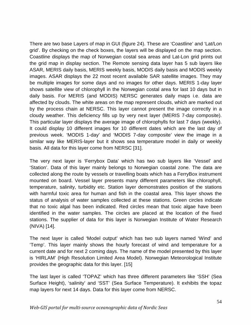
54 Web-GIS portal for multi-source oceanographic data of Nordic Seas
There are two base Layers of map in GUI (figure 24). These are ‘Coastline’ and ‘Lat/Lon grid’. By checking on the check boxes, the layers will be displayed on the map section. Coastline displays the map of Norwegian costal sea areas and Lat-Lon grid prints out the grid map in display section. The Remote sensing data layer has 5 sub layers like ASAR, MERIS daily basis, MERIS weekly basis, MODIS daily basis and MODIS weekly images. ASAR displays the 22 most recent available SAR satellite images. They may be multiple images for some days and no images for other days. MERIS 1-day layer shows satellite view of chlorophyll in the Norwegian costal area for last 10 days but in daily basis. For MERIS (and MODIS) NERSC generates daily maps i.e. data are affected by clouds. The white areas on the map represent clouds, which are marked out by the process chain at NERSC. This layer cannot present the image correctly in a cloudy weather. This deficiency fills up by very next layer (MERIS 7-day composite). This particular layer displays the average image of chlorophylls for last 7 days (weekly). It could display 10 different images for 10 different dates which are the last day of previous week. ‘MODIS 1-day’ and ‘MODIS 7-day composite’ view the image in a similar way like MERIS-layer but it shows sea temperature model in daily or weekly basis. All data for this layer come from NERSC [31]. The very next layer is ‘Ferrybox Data’ which has two sub layers like ‘Vessel’ and ‘Station’. Data of this layer mainly belongs to Norwegian coastal zone. The data are collected along the route by vessels or travelling boats which has a FerryBox instrument mounted on board. Vessel layer presents many different parameters like chlorophyll, temperature, salinity, turbidity etc. Station layer demonstrates position of the stations with harmful toxic area for human and fish in the coastal area. This layer shows the status of analysis of water samples collected at these stations. Green circles indicate that no toxic algal has been indicated. Red circles mean that toxic algae have been identified in the water samples. The circles are placed at the location of the fixed stations. The supplier of data for this layer is Norwegian Institute of Water Research (NIVA) [14]. The next layer is called ‘Model output’ which has two sub layers named ‘Wind’ and ‘Temp’. This layer mainly shows the hourly forecast of wind and temperature for a current date and for next 2 coming days. The name of the model presented by this layer is ‘HIRLAM’ (High Resolution Limited Area Model). Norwegian Meteorological Institute provides the geographic data for this layer. [15] The last layer is called ‘TOPAZ’ which has three different parameters like ‘SSH’ (Sea Surface Height), ‘salinity’ and ‘SST’ (Sea Surface Temperature). It exhibits the topaz map layers for next 14 days. Data for this layer come from NERSC.

55 Web-GIS portal for multi-source oceanographic data of Nordic Seas
5.2. New modifications in DISPRO Now it is time to describe that what are the new features which are added in this thesis related to the old DISPRO system? The old DISPRO has used daily updated fixed files as storage place of geographic data. There was no oceanographic data base in this system. A Master thesis completed in 2007 developed a prototype to observe oil spills in the Barents and Kara seas. [21] So far main focus was on Barents Sea and Kara sea areas. The figure 26 shows the overall pictorial view of existing DISPRO.
Fig 26: The pictorial view of old DISPRO [21]
This thesis has added some new features in DISPRO. The table 6 shows a comparative difference between DISPRO and Web GIS DISPRO. That is, Web base GIS system will mainly deal with Nordic Seas areas and it has a spatially enabled oceanographic

56 Web-GIS portal for multi-source oceanographic data of Nordic Seas
database for large number of in-situ data provided by various source projects (see figure 5). Stations positions are not only belong to coastal area of Norway but also in all over Nordic Seas (Norwegian Sea, the Greenland Sea and the Iceland Sea). After loading those data in the spatially enabled database (chapter 4) and by accessing through MapServer the system would capable to display all the positions of the stations with selected some symbol in the ‘Map’ section (figure 24) as GUI in the DISPRO. The new system is not only display the oceanographic information of recent years but also competent to view information of last few decades. So user can get an overview about Nordic Seas that how the condition was in those particular sea areas.
DISPRO WEB GIS DISPRO
1. Action area Barents Sea and Kara
Sea.
2. Satellite data (ASAR, MERIS, MODIS,
AMSR) and met-ocean model forecast
(Topaz).
3. Used fixed file/ daily basis updated file
data so far and OPeNDAP protocol.
4. All data can be overlaid on the same
map, zoom and pan or layer toggling.
1. Action area Nordic Sea, Greenland,
Iceland and few areas of Barents Sea.
2. New source of oceanographic data from
“The Nordic Seas in the Global Climate
System” and from many others.
3. Using a dedicated spatially enabled
oceanographic database.
4. It is capable to automatically point out
the position of the stations on the map.
Table 6: Difference between DISPRO 3 [21] and Web GIS DISPRO
The client-server model with database architecture has been implemented in this thesis. The figure 27 presents a view of system design. Client submit request through a HTML request form and send it to HTTP Server who process the request together with MapServer. If client needs any data from database container then Server forward the request to database (ODB) and ODB sends back response with required data to the server. Finally server generates a response to the client as per its request.

57 Web-GIS portal for multi-source oceanographic data of Nordic Seas
Fig 27: New system view
The figure 28 illustrates how client-server architecture has merged with DISPRO. An
HTML request form has added as client with the same MapServer used by existing
DISPRO and also a spatially enabled oceanographic database (MySQL) is connected
with MapServer. As discussed in chapter 2, the project named ‘Nordic Seas in the
Global Climate’ has developed oceanographic databases which have three different
databases. They are quality controlled merged initial database, objectively analysed and
interpolated database, and objectively analysed monthly fields database. A separate
ODB was developed after taking the data from the above mentioned project. The data
were supplied for this thesis from their second database (interpolated database). The
ODB of this thesis contains all stations oceanographic data with few selected
parameters of the year 2006. MapServer reads the map file with all specifications send
by client and fetch data from the database and display the image in the browser as GUI.
All figures in the fig 24 marked by red color ‘NEW’ is the newly added design.

58 Web-GIS portal for multi-source oceanographic data of Nordic Seas
Fig 28: The new architecture of Web GIS DISPRO [21]

59 Web-GIS portal for multi-source oceanographic data of Nordic Seas
5.3. Working with GUI
MAPFILE C:/Matadata/cities.map
REQUEST GetMap
SERVICE WMS
VERSION 1.1.1
LAYERS cities,border2
STYLES default
SRS EPSG:4326
BBOX -90,180,90,180
WIDTH 800
HEIGHT 600
FORMAT image/png
Submit
Fig 29: HTML request generating form
A HTML form was created for submitting request by client (fig 29). The form has many different fields named MAPFILE, REQUEST, SERVICE, VERSION, LAYER, STAYELS, SRS, BBOX, WIDTH, HEIGHT and FORMAT. MAPFILE gets the name of the map file to be execute, SERVICE tells which map services should follow by the map server (WMS/WFS), VERSION tells the version number of service, LAYERS tells about which layer inside the map file should execute by the MapServer, SRS (Spatial Reference System) says details about map projections, BBOX (bounding box) illustrates specific bounds of a map by latitude-longitude, WIDTH and HIGHT says about width and height of the map and format tells about the image type of the map. Client generates a request by clicking the ‘Submit’ button. HTML reads the location of MapServer under the key word ‘action’ (fig 26) and then all other requested specifications go directly to the MapServer.

60 Web-GIS portal for multi-source oceanographic data of Nordic Seas
<html><head> </head><body bgcolor="white"> <form action="http://127.0.0.1/cgi-bin/mapserv.exe" method="get" > * * * </form>
Fig 30: a piece of HTML code pointing to MapServer
Like database, GUI also tested with an example map file called ‘cities.map’ (Appendix 1). It has mentioned the layer details, projection details, symbols details and database connection details inside the cities.map file. Now if client submits the request form with all different specifications then the browser will display the map like below. The fig 27 shows three stars which are the position of the cities according to the latitude and longitude on the map. For the testing purpose the ‘cities’ table under ‘nsdb’ database has only three data. The entire blue coloured maps are the polygon type data from the ‘border2’ table under the same database.
Fig 31: Positions of the cities on the map
61 Web-GIS portal for multi-source oceanographic data of Nordic Seas
5.4. Result
As shown in the previous section, GUI is working for ‘cities.map’ file and with ‘nsdb’ spatial database. It has already been conferred that how ‘dispro’ typical database could be changed into spatially enabled database in the chapter 4. Then it is not hard to say that it must work for some map file with ‘dispro’ database. It can be possible to point out the position of the stations with other symbols like circle or ellipse but not definitely similar to cities map file (star symbol). Thus the first requirement in GUI of this thesis is achieved. To implement the other small part of GUI, we need to introduce another map feature called Web Features Service (WFS) which can create dynamic clickable map. This dynamic map can display all oceanographic parameters with numeric models. The detail about it will be discussed in chapter 6.

62 Web-GIS portal for multi-source oceanographic data of Nordic Seas
Chapter 6 Discussions and Challenges
6.1. Discussion Details study in this field shows there exist certain number of oceanographic web-based GIS system, capable to display oceanographic information. DISPRO as a part of InterRisk project has tried to make the Web-GIS system on its own way i.e. to make a marine monitoring system in a user friendly manner. Though this system is not an open source but it well be used for marine or coastal management purpose in a broad sense. It has been tried to develop this Web GIS system with most modern open source software and tools which really suit with this thesis and does not make it complicated. Many others features could be added to enhance this system later on. Those extra features which could be added in the future, will be discussed in the very next chapter. In this section it will be evaluated that how far developer has managed to achieve the user/customer requirements. Though the tasks of the thesis were quite big for a master thesis, the developer has managed to achieve most of the requirements; and also has the full idea for doing a small reaming part. Now it’s time to discuss the all achieved user requirements one by one here in below:
An oceanographic Database (ODB) It was the first requirement of the customer. So far DISPRO did not have any separate oceanographic database for oceanographic data or in-situ data. The aim of DISPRO is to handle not only satellite monitoring of Barents and Kara Seas [21] but also enlarge the system to have a vast idea about various oceanographic parameters of a very large sea area like Nordic Seas for last many decades. So it was necessary to create an Oceanographic database (ODB) with data from Nordic Seas. Fortunately Nansen Center (NERSC) has another project [25] which supplies the oceanographic data very promptly. After receiving the oceanographic data, it was important to analyze the data to form a database. As mentioned earlier, data collected in two different ways named profiling floats (PF) and research vessels (RV) were merged in a single database because they were the similar data but gathered using different instruments. The relations were searched out among the different parameters and the table were formed. Initially data were contained in a text file (.dat form) with tab separated columns. To upload the data easily in the ODB, the file format had to be changed in CSV (Comma separated Values)

63 Web-GIS portal for multi-source oceanographic data of Nordic Seas
format with .csv file name extension. MySQL offers some easy query (LOAD DATA LOCAL INFILE) [6] to upload the comma separated data column by column from a CSV file. Otherwise, it is a very hard job to upload large number (2980) of data in a database manually. The query and reply from the database is shown below. mysql> use dispro Reading table information for completion of table and column names Database changed mysql> LOAD DATA LOCAL INFILE '/mnt/fritjof/wms/nsdb/station.csv' INTO TABLE STATION FIELDS TERMINATED BY ','; Query OK, 2980 rows affected, 8346 warnings (0.94 sec) Records: 2980 Deleted: 0 Skipped: 0 Warnings: 7171
Fig 32: Loading data in the database through query
The connectivity issue between ODB and MapServer was discussed briefly in chapter 4. The update frequency of ODB will be in irregular basis since the field experiments by cruises or vessels are carried out at different times and they collect oceanographic data with different parameters. Also, new data may become available from other sources like research institutions or from other project works at different times. So ODB had to be able to receive the updates manually when there is some new data.
Spatially Enabled Database The spatially enabled database is the main pillar of this thesis. When developer was searching for a real solution, at that time concept of spatial enabled database was arrived like an angle and it built the path for rest of the thesis. So this thesis is fully dependent on the spatially enabled oceanographic database. The detail about spatial enabled database has already been discussed in chapter 4.
Problems in Linux Platform As mentioned earlier developer attempted several times to work in Linux environment and also customer‘s first preference was the same. But due to some unknown reason the proposed technology did not work. According to the documentation [42] of MySQL, MapServer and GDAL the technology definitely work in Linux operating system. But the reason for the technology not working was quite surprise to the developer and

64 Web-GIS portal for multi-source oceanographic data of Nordic Seas
customer. Due to the time boxing factor developer had to move to another platform rather than investigating the real cause of the old technologies not working. It's important to discuss how the developer has attempted to work on the Linux platform. To create connectivity between MySQL and MapServer installed in Linux server [1], there needs a small XML file with ‘.ovf’ (Open Virtualization Format) file extension, in case this ovf file (fig 33) is called ‘connection.ovf’. If one looks at the connection string under the tag <SrcDataSource>, the MySQL database name is ‘dispro’; and ‘STATION’ is the name of the table containing the coordinate data. Host and port names are of MySQL server. The GeometryField element needs to tell OGR which fields store the x and y coordinate data in the table. The GeometryType element tells that the vector data are of WKB geometry types. <OGRVRTDataSource> <OGRVRTLayer name="nsdb"> <SrcDataSource>MYSQL:dispro,user=****,password=****, host=johansen.nersc.no,port=3306, tables=STATION </SrcDataSource> <SrcSQL>SELECT absnum, stlat, stlon FROM STATION</SrcSQL> <GeometryType>wkbPoint</GeometryType> <GeometryField encoding="PointFromColumns" x="stlon" y="stlat"/> </OGRVRTLayer> </OGRVRTDataSource>
Fig 33: connection.ovf file
To test that the connection has created between database and MapServer, one should run the command below from terminal window. Ogrinfo /mnt/fritjof/wms/nsdb/phapal/connection.ovf The OGR (OpenGIS Simple Features Reference Implementation) is a Simple Features library of C++ library which has the ability to read or often write different types of vector file formats like ESRI Shapefiles, PostGIS, Oracle Spatial, Mapinfo MID/MIF and TAB formats etc. OGR (ogrinfo) is also a commandline tool which displays all information about an OGR supported data source in a listed form. OGC has made the ‘Simple Features’ conditions and has established certain standards for adding spatial functionality to database system. Actually OGR is a sub library of GDAL parent library which is a translator library for raster geo-spatial data formats. So main thing is that

65 Web-GIS portal for multi-source oceanographic data of Nordic Seas
OGR works for Vector data and GDAL works for raster data. GDAL/OGR has full support for MySQL database [3] and needs to install in the system with MapServer. Let’s come back in the discussion about ogrinfo command. Initially it returned failure (fig 34 (i)) i.e. MapServer was unable to create connection with database. The problem was that ogrinfo was not installed with MySQL support. Such support is not included by default since it needs a MySQL driver. After installing driver for MySQL the command ‘ogrinfo -format’ was run and finally it showed driver support for MySQL (fig 34(ii)).
(i) (ii) Fig 34: (i) Reply from ogrinfo command before driver installation for MySQL (ii) Reply from ‘ogrinfo –formats’ command after driver installation for MySQL Now if one runs the command ‘ogrinfo fritjof/wms/nsdb/connection.ovf’, it returns like below. The ERROR 4 is just telling that it is a read-only driver. ERROR 4: Update access not supported for VRT datasources. Had to open data source read-only. INFO: Open of `/mnt/fritjof/wms/nsdb/conionnnect.ovf' using driver `VRT' successful. 1: nsdb (Point)
FAILURE: Unable to open datasource `/mnt/fritjof/wms/nsdb/phapal/ connection.ovf' with the following drivers. -> ESRI Shapefile -> MapInfo File -> UK. NTF -> SDTS -> TIGER -> S57 -> DGN -> VRT -> AVCBin -> REC -> Memory -> CSV -> GML
Ogrinfo –formats Supported Formats: -> "ESRI Shapefile" (read/write) -> "MapInfo File" (read/write) -> "UK .NTF" (readonly) -> "SDTS" (readonly) -> "TIGER" (read/write) -> "S57" (read/write) -> "DGN" (read/write) -> "VRT" (readonly) -> "REC" (readonly) -> "Memory" (read/write) -> "BNA" (read/write) -> "CSV" (read/write) -> "GML" (read/write) -> "GPX" (read/write) -> "KML" (read/write) -> "GeoJSON" (read/write) -> "GMT" (read/write) -> "MySQL" (read/write) # Now it is showing but previously it was missing # -> "AVCBin" (readonly)

66 Web-GIS portal for multi-source oceanographic data of Nordic Seas
To display the data stored in the database on the map, it needs to mention the name of ‘connection.ovf’ file inside the map file under the key word CONNECTION like below and the ovf file should in the same directory otherwise one has to tell the whole class path. LAYER . . . . . . . CONNECTION "connection.ovf" # mentioning the name of ovf file. DATA "nsdb" PROJECTION "init=epsg:4326" . . . . . . . END After doing all above mentioned procedures developer sent a request to the MapServer with filling all required fields of the HTML form (figure 29), but MapServer displayed a blank page without any map. MapServer did neither throw any error message nor display any map. GDAL documentation [42] says “This driver implements read and write access for spatial data in MySQL tables. This functionality was included in GDAL/OGR 1.3.2” and “Versions older than 5.0.16 of MySQL are known to have issues with some WKB generation and may not work properly”. But developer used MapServer version 4.10.3, GDAL version 1.5.3 and MySQL version 5.0.45 which are quite newer version than the mentioned versions in the GDAL documentation. According to available information MapServer should display the map and the station positions in the map. After detail study of MapServer tutorial [28], MapServer users request mailing lists [2], MapServer developer mailing list [2] and MySQL official site [11] developer did not get any satisfactory answer about failure of the technologies. It could be happen that GDAL driver does not offer this facility any more for the newer version of MySQL. But developer is not exactly sure about it.
The remaining part of GUI So far developer had used Web Map Services (WMS) to display the maps by the help of MapServer. WMS version 1.1.1 displays only static gridded maps which do not offer the on-click features for the users. This static map does not fulfill the remaining GUI requirements. To solve this purpose developer needs to introduce dynamic map services. But MapServer supports other services called Web Features Services (WFS) which can create dynamic maps which are clickable. The command ‘mapserv -v’ returns the all supported software and tools by MapServer. The highlighted portion
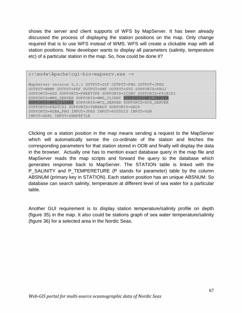
67 Web-GIS portal for multi-source oceanographic data of Nordic Seas
shows the server and client supports of WFS by MapServer. It has been already discussed the process of displaying the station positions on the map. Only change required that is to use WFS instead of WMS. WFS will create a clickable map with all station positions. Now developer wants to display all parameters (salinity, temperature etc) of a particular station in the map. So, how could be done it?
c:\ms4w\Apache\cgi-bin>mapserv.exe -v
MapServer version 5.2.1 OUTPUT=GIF OUTPUT=PNG OUTPUT=JPEG OUTPUT=WBMP OUTPUT=PDF OUTPUT=SWF OUTPUT=SVG SUPPORTS=PROJ SUPPORTS=AGG SUPPORTS=FREETYPE SUPPORTS=ICONV SUPPORTS=FRIBIDI SUPPORTS=WMS_SERVER SUPPORTS=WMS_CLIENT SUPPORTS=WFS_SERVER SUPPORTS=WFS_CLIENT SUPPORTS=WCS_SERVER SUPPORTS=SOS_SERVER SUPPORTS=FASTCGI SUPPORTS=THREADS SUPPORTS=GEOS SUPPORTS=RGBA_PNG INPUT=JPEG INPUT=POSTGIS INPUT=OGR INPUT=GDAL INPUT=SHAPEFILE
Clicking on a station position in the map means sending a request to the MapServer which will automatically sense the co-ordinate of the station and fetches the corresponding parameters for that station stored in ODB and finally will display the data in the browser. Actually one has to mention exact database query in the map file and MapServer reads the map scripts and forward the query to the database which generates response back to MapServer. The STATION table is linked with the P_SALINITY and P_TEMPERETURE (P stands for parameter) table by the column ABSNUM (primary key in STATION). Each station position has an unique ABSNUM. So database can search salinity, temperature at different level of sea water for a particular table. Another GUI requirement is to display station temperature/salinity profile on depth (figure 35) in the map. It also could be stations graph of sea water temperature/salinity (figure 36) for a selected area in the Nordic Seas.

68 Web-GIS portal for multi-source oceanographic data of Nordic Seas
Fig 35: Station temperature-depth profile [8]
Fig 36: Station graph of salinity for a large area of Nordic Sea [32]

69 Web-GIS portal for multi-source oceanographic data of Nordic Seas
To implement this type of figure in to GUI in this system one needs to use some WFS plotting components for example ‘plowfs’ which is developed by Polymouth Marine Laboratory, UK [4]. At present plowfs can only plot time series. With some modification it should be able to plot depth profiles like in Figure 35. Making a contact plot with plowfs will require significantly larger changes to this plotting component. It has to be installed in the system with MapServer. By selecting a large area in the map by mouse pointer and right click on the selected area user can choose the different parameters from the list, and user has to make a request to MapServer by selecting one parameter. Before that developer has to fix a scaling according the range of the parameters. Let’s take salinity as an example. Developer can make a scale for different range of salinity like 0-5, 5-10, 10-15 (psu is the unit of salinity) etc by corresponding different colors. Now developer has to mention the database query to search data with various ranges from the database and also developer needs to say to the MapServer the various colors for the corresponding range of salinity inside a map file. Then MapServer will be able to display the stations graph for salinity.
6.2. Challenges
In this section, the challenges during the software development process are described briefly. Every software development process consist some challenges and this thesis was not an exception. According to the developer the following points could be considered as challenges for this thesis.
• New types of work
o The tasks of this thesis were totally new and developer had to become familiar with all necessary tools and technologies.
• Work with maps
o Mainly the tasks were to work with digital maps. It was also necessary to display many static or dynamic maps as geographical user interface.
• Initial problems with software versions and tool drivers
o As stated earlier, developer had few problems with the version supports and driver supports of required software and tools.

70 Web-GIS portal for multi-source oceanographic data of Nordic Seas
• Time consuming during upgrading software in server
o Software up gradation in server is always time consuming process.
Usually many other developers or other departments access the same server and it is quite impossible to protect the accessibility of other people during upgrading period on their working hours.
• Changing of database many times
o As said earlier, developer had to experiment with databases and their data types. Developer had to move from typical MySQL tables to spatially enabled database.
• Changing of Platform (Linux Windows)
o The software platform (operating system) had to change at the mid way of development process due to major problems with GUI. It was big challenge for the developer to familiar with new environment and proceeds further.
• Time management problem
o Due to many changes in software and technologies during development process, lots of time was spent managing new situations. It was very hard to fulfil all user requirements with in the stipulated time frame.
• Shortage of literature and web help in this field
o According to this thesis developer, it was realized that there are certain shortage of literature and web helps. There are not many good books available for GIS development and few books are back dated in new version of software.

71 Web-GIS portal for multi-source oceanographic data of Nordic Seas
Chapter 7 Conclusion
As discussed before there exist many different web-based oceanographic GIS systems, to provide more and more geographical information to the users. DISPRO web GIS system was developed progressively as an active part of InterRisk project. DISPRO system utilizes data which are collected by NERSC but also collect by many other sources and uses open source software and tools. These specifications add new excellences in this thesis as a part of DISPRO. Today DISPRO is quite large web based GIS, distributed marine information monitoring and management system including all different parts. Definitely DISPRO has the full potencies to become a world class web based oceanographic GIS system. It is very much possible to add many other new features to enhance the web based GIS system DISPRO. We could include more parameters like pH, HAB, dissolved CO2 and O2 in sea water. The range of time periods of in-situ/ marine data could be increased in the ODB. This thesis used the available oceanographic data only from the year 2006 but the time period could be enlarged backwards up to many decades, e.g. so far data are on hand for the period 1877- 2007 [25]. ODB will have the capacity to receive updates whenever there is some new data. New GUI also could be added in to this system. We could comprise more station graphs, numerical models and time series for various parameters. We could make some numerical model/graph versus time period (time series) or animated model to represent the major changes in sea water parameters have occurred for a station or a particular area in Nordic Seas since the last century due to the global warming. I have learned and understood a lot of new technologies during working in this thesis. The subject of this thesis is very comprehensive, and the learning curve has been vertical. I have gained knowledge in handling spatial oceanographic data and developing on-line geographical information system. I topic of this thesis was very new to me when I started, but I had been become familiar with it as time passed. I liked this thesis because I have found out many new terminologies which polished my skills and gave me motivation and courage for my future professional carrier. To draw conclusion the developer could say, though the objectives for this thesis has been completed successfully but needs more time to merge all the things together with DISPRO before open for the users to use. But the main goal is achieved i.e. web-based GIS system for multi-source geography data could become a reality through this thesis.
72 Web-GIS portal for multi-source oceanographic data of Nordic Seas
References
[1]. http://www.mapserver.org/input/vector/mysql.html (20.05.2009) [2] http://lists.osgeo.org/mailman/listinfo/mapserver-dev/ (20.05.2009) [3]. http://www.gdal.org/ogr/ogr_formats.html (20.05.2009) [4]. http://www.pml.ac.uk/ (20.05.2009) [5]. http://www.maptools.org/ms4w/ (20.05.2009) [6]. http://www.modwest.com/help/kb6-253.html (20.05.2009) [7]. http://en.wikipedia.org/wiki/Comparison_of_relational_database_ management_systems [8]. http://cimss.ssec.wisc.edu/sage/oceanography/lesson4/images/ sm_temperature_depth.jpg (20.05.2009) [9]. http://dispro.ucc.ie/apps/dismar/index.xml (20.05.2009) [10]. http://wms.nersc.no/norway/regions.xml (20.05.2009) [11]. www.mysql.com (20.05.2009) [12]. Sandven and Johannessen, 2006 [13]. Johannessen et al., 2007 [14]. www.niva.no (20.05.2009) [15]. www.met.no (20.05.2009) [16]. Johannenssen O.M, L.H Pettersson, A. Korablev, V. Volkov and co-authers.. 2007: The Nordic Seas in the global climate. Final report to INTAS grant 03-51-4620, July 2007. [17]. http://www.esri.com/library/whitepapers/pdfs/shapefile.pdf [18]. http://www.intas.be/ (20.05.2009), Home page of INTAS. [19] http://www.nersc.no/dismar/ (20.05.2009) [20] http://interrisk.nersc.no/ (20.05.2009) [21] Oleksandr Kit, "Implementation of Web-mapping technologies for satellite monitoring and management of Barents and Kara seas", Master Thesis, University of Bergen, 7 March 2007. [22] W3C; http://www.w3c.org/ (20.05.2009) [23] Open Geospatial Consortium; www.opengeospatial.org (20.05.2009) [24] ISO 19115; http://www.isotc211.org/scope.htm#19115 (20.05.2009) [25] Alexander A. Korablev, Ola M. Johannessen and others: Oceanographic database and climatology compilation for the ocean climate monitoring in the Nordic Sea, 2008. (Paper in peparation) [26] http://cordis.europa.eu/fp7/ict/home_en.html (20.05.2009)
73 Web-GIS portal for multi-source oceanographic data of Nordic Seas
[27] Robert 0. Harger and Can Korman; A BASIS FOR SAR OCEANOGRAPHY: THEORY AND EXPERIMENT [28] UMN MapServer home site: http://mapserver.org/ (20.05.2009) [29] Object-Oriented Software Engineering: Practical Software Development using UML and Java by Timothy C. Lethbridge and Robert Laganière, First edition. [30] http://era.nih.gov/docs/rup_fundamentals_slide03.jpg (20.05.2009) [31] NERSC Home site; www.nersc.no (20.05.2009) [32] Alexander Korablev, Presentation at ARCWARM Meeting (14.02.2008). [33] http://cnx.org/content/m14619/latest/graphics1.png (20.05.2009) [34] http://www.methodsandtools.com/archive/TDD1.jpg (20.05.2009) [35] http://www.agilemanifesto.org/ (20.05.2009) [36] http://www.agilealliance.org/ (20.05.2009) [37] Robert Cecil Martin (Uncle Bob); Agile Software Development Principle, Patterns, and Principles; Prentice Hall. [38] http://www.intevation.de/~jan/gen2shp (20.05.2009) [39] http://dev.mysql.com/tech-resources/articles/4.1/gis-with-mysql.html (20.05.2009) [40] http://en.wikipedia.org/wiki/Spatial_database (20.05.2009) [41] http://shapelib.maptools.org/ [42] http://www.gdal.org/ogr/drv_mysql.html (20.05.2009) [43] http://www.gdal.org/ ; GDAL home page (20.05.2009) [44] http://www.esri.com/software/arcgis/arcinfo/index.html (20.05.2009) [45] http://spatialreference.org/ref/epsg/4326/ (20.05.2009)

74 Web-GIS portal for multi-source oceanographic data of Nordic Seas
Appendix 1 Contents of ‘cities.map’ file: MAP CONFIG "MS_ERRORFILE" "/ms4w/tmp/ms_error_cities.txt" NAME "MYSQL-TEST" EXTENT -180 -90 180 90 UNITS dd CONFIG "CPL_DEBUG" "ON" DEBUG 5 SIZE 500 500 IMAGETYPE PNG OUTPUTFORMAT NAME PNG DRIVER "GD/PNG" MIMETYPE "image/png" IMAGEMODE PC256 EXTENSION "png" END PROJECTION "init=epsg:4326" END SHAPEPATH "/mnt/fritjof/wms/nsdb" WEB LOG "/tmp/ms_error_cities.txt" END SYMBOL Name 'star' Type VECTOR Filled TRUE Points 0 .375 .35 .375 .5 0 .65 .375 1 .375 .75 .625 .875 1 .5 .75 .125 1 .25 .625 END END
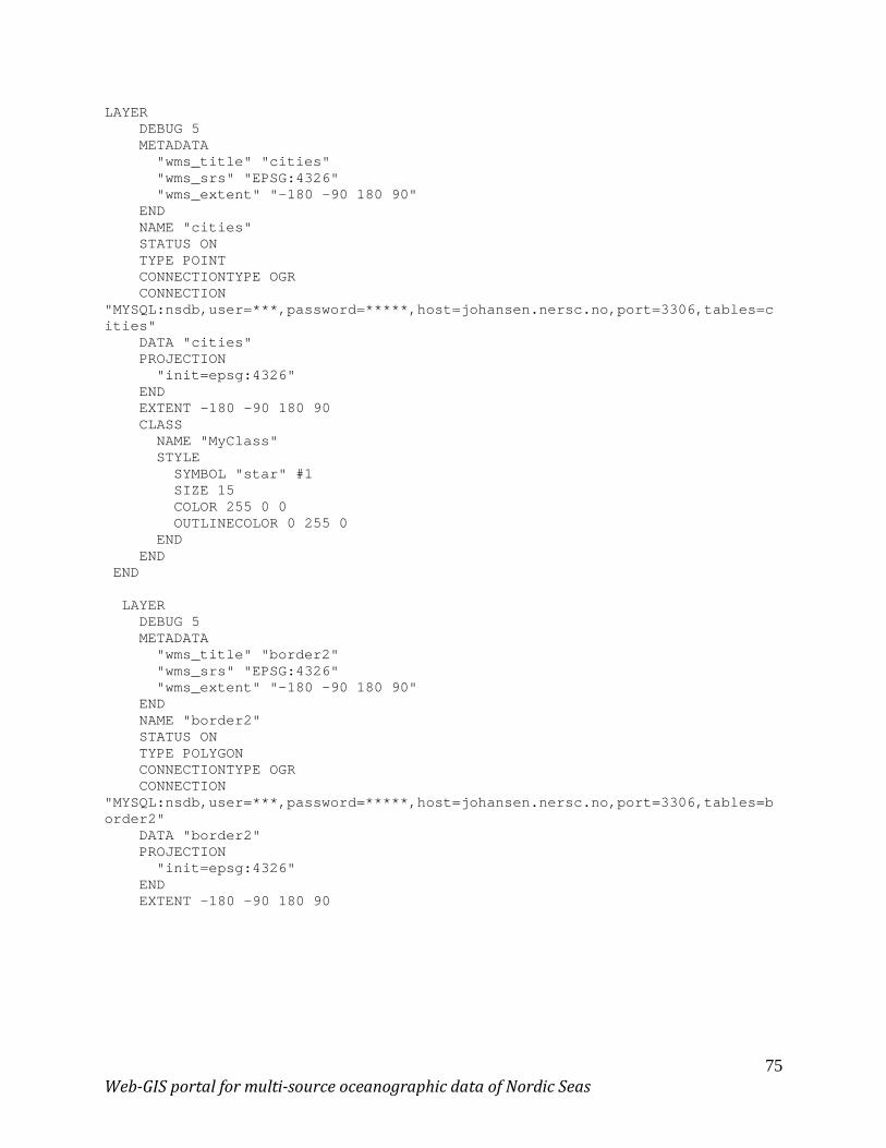
75 Web-GIS portal for multi-source oceanographic data of Nordic Seas
LAYER DEBUG 5 METADATA "wms_title" "cities" "wms_srs" "EPSG:4326" "wms_extent" "-180 -90 180 90" END NAME "cities" STATUS ON TYPE POINT CONNECTIONTYPE OGR CONNECTION "MYSQL:nsdb,user=***,password=*****,host=johansen.nersc.no,port=3306,tables=cities" DATA "cities" PROJECTION "init=epsg:4326" END EXTENT -180 -90 180 90 CLASS NAME "MyClass" STYLE SYMBOL "star" #1 SIZE 15 COLOR 255 0 0 OUTLINECOLOR 0 255 0 END END END LAYER DEBUG 5 METADATA "wms_title" "border2" "wms_srs" "EPSG:4326" "wms_extent" "-180 -90 180 90" END NAME "border2" STATUS ON TYPE POLYGON CONNECTIONTYPE OGR CONNECTION "MYSQL:nsdb,user=***,password=*****,host=johansen.nersc.no,port=3306,tables=border2" DATA "border2" PROJECTION "init=epsg:4326" END EXTENT -180 -90 180 90

76 Web-GIS portal for multi-source oceanographic data of Nordic Seas
CLASS NAME "MyClass" COLOR 0 0 255 #STYLE #SYMBOL 1 #SIZE 15 #COLOR 255 0 0 #OUTLINECOLOR 0 255 0 #END END END LAYER # Grid line layer begins here METADATA "wms_srs" "EPSG:9810 EPSG:4326 EPSG:50000" "wms_title" "Grid" "wms_layer_group" "/vector/base" "wms_keywordlist" "datestamp: 2005-06-08, grid lines, graticule layer" "wms_extent" "-180 -90 180 90" # global "wms_group_title" "Base Layers" "wms_abstract" "This is the graticule layer" END NAME "grid" TYPE LINE STATUS ON CLASS NAME "Graticule" COLOR 113 166 218 LABEL COLOR 155 0 0 SIZE MEDIUM POSITION AUTO PARTIALS FALSE BUFFER 5 OUTLINECOLOR 255 255 255 END END PROJECTION "init=epsg:4326" # Geographic longitude-latitude projection END GRID MAXSUBDIVIDE 1 MINSUBDIVIDE 64 MAXSUBDIVIDE 64 LABELFORMAT "DDMM" END END # Grid line layer ends here END
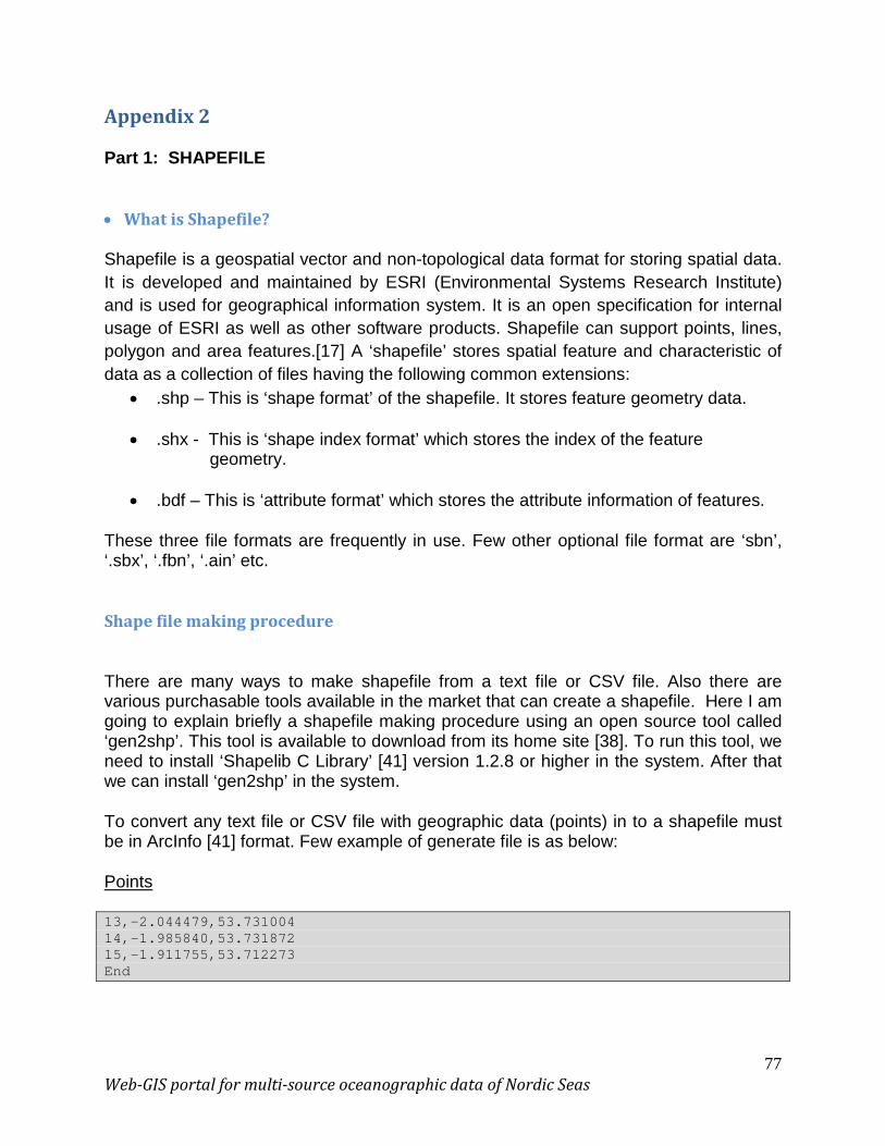
77 Web-GIS portal for multi-source oceanographic data of Nordic Seas
Appendix 2 Part 1: SHAPEFILE • What is Shapefile? Shapefile is a geospatial vector and non-topological data format for storing spatial data. It is developed and maintained by ESRI (Environmental Systems Research Institute) and is used for geographical information system. It is an open specification for internal usage of ESRI as well as other software products. Shapefile can support points, lines, polygon and area features.[17] A ‘shapefile’ stores spatial feature and characteristic of data as a collection of files having the following common extensions:
• .shp – This is ‘shape format’ of the shapefile. It stores feature geometry data.
• .shx - This is ‘shape index format’ which stores the index of the feature geometry.
• .bdf – This is ‘attribute format’ which stores the attribute information of features.
These three file formats are frequently in use. Few other optional file format are ‘sbn’, ‘.sbx’, ‘.fbn’, ‘.ain’ etc.
Shape file making procedure
There are many ways to make shapefile from a text file or CSV file. Also there are various purchasable tools available in the market that can create a shapefile. Here I am going to explain briefly a shapefile making procedure using an open source tool called ‘gen2shp’. This tool is available to download from its home site [38]. To run this tool, we need to install ‘Shapelib C Library’ [41] version 1.2.8 or higher in the system. After that we can install ‘gen2shp’ in the system.
To convert any text file or CSV file with geographic data (points) in to a shapefile must be in ArcInfo [41] format. Few example of generate file is as below:
Points
13,-2.044479,53.731004 14,-1.985840,53.731872 15,-1.911755,53.712273 End

78 Web-GIS portal for multi-source oceanographic data of Nordic Seas
We will take staion.csv file as an example and will convert it in to Shapefile. bash-3.00$ cat station.csv # ABSNUM, STFLAG, STLAT, STLON, STDATE, STTIME 851342,1,64.18417,-51.768,23.03.2006,16:50:00 851343,1,64.26667,-51.65117,23.03.2006,18:19:00 851345,1,64.1155,-51.88467,15.05.2006,13:50:00
First step is to separate the co-ordinate data from the attribute data (N.B. the grep command remove lines with ‘#’) bash-3.00$ cut –d, -f 1,3,4 < station.csv | grep –v ‘#’ > station.gen bash-3.00$ cat station.gen 851342,64.18417,-51.768 851343,64.26667,-51.65117 851345,64.1155,-51.88467 Now we have to make attribute file (.att) which contains the header information. bash-3.00$ cut –d, -f 1,2,5,6 < station.csv > station.att bash-3.00$ cat station.att # ABSNUM, STFLAG,STDATE, STTIME 851342,1,23.03.2006,16:50:00 851343,1,23.03.2006,18:19:00 851345,1,15.05.2006,13:50:00 The shape file now created now with gen2shp. [38] bash-3.00$ gen2shp test points < station.gen bash-3.00$ ls -l test.* -rw-rw-r-- 1 jan intevati 113 25. May 18:30 test.dbf -rw-rw-r-- 1 jan intevati 212 25. May 18:30 test.shp -rw-rw-r-- 1 jan intevati 132 25. May 18:30 test.shx Now the test.dbf file needs to be replaced by the attribute file.
79 Web-GIS portal for multi-source oceanographic data of Nordic Seas
Part 2: Map Projection
A map projection is a method to representing all or part of the round Earth on plane. That is, map projection is way to characterize image of the earth onto paper or computer screen. To do this there needs some deformation. Every projection has its few advantages and disadvantages. There is unlimited numbers of achievable map projections and the concept is there is no "best" projection. The map developer should select one which fits best.
EPSG:4326
The World Geodetic System (WGS) is a standard co-ordinate frame for representing Earth as ellipsoid surface. The current version of WGS is 84. EPSG: 4326 is a coordinate system for latitude and longitude; and it refers to WGS84. The specifications of EPSG:4326 is as below: EPSG:4326 [44]
Refer to WGS 84
• WGS84 Bounds: -180.0000, -90.0000, 180.0000, 90.0000 • Projected Bounds: -180.0000, -90.0000, 180.0000, 90.0000 • Scope: Horizontal component of 3D system. • Last Revised: 2007-08-27 • Area: World