Weather types across the Maritime Continent: from the ...

HAL Id: hal-02895055https://hal.archives-ouvertes.fr/hal-02895055

Submitted on 15 Sep 2021

HAL is a multi-disciplinary open accessarchive for the deposit and dissemination of sci-entific research documents, whether they are pub-lished or not. The documents may come fromteaching and research institutions in France orabroad, or from public or private research centers.

L’archive ouverte pluridisciplinaire HAL, estdestinée au dépôt et à la diffusion de documentsscientifiques de niveau recherche, publiés ou non,émanant des établissements d’enseignement et derecherche français ou étrangers, des laboratoirespublics ou privés.

Distributed under a Creative Commons Attribution| 4.0 International License

Weather types across the Maritime Continent: from thediurnal cycle to interannual variations

Vincent Moron, Andrew Robertson, Jian-Hua Qian, Michael Ghil

To cite this version:Vincent Moron, Andrew Robertson, Jian-Hua Qian, Michael Ghil. Weather types across the MaritimeContinent: from the diurnal cycle to interannual variations. Frontiers in Environmental Science,Frontiers, 2015, 2, �10.3389/fenvs.2014.00065�. �hal-02895055�

https://hal.archives-ouvertes.fr/hal-02895055

http://creativecommons.org/licenses/by/4.0/


https://hal.archives-ouvertes.fr

ORIGINAL RESEARCH ARTICLEpublished: 13 January 2015

doi: 10.3389/fenvs.2014.00065

Weather types across the Maritime Continent: from thediurnal cycle to interannual variationsVincent Moron1,2*, Andrew W. Robertson2, Jian-Hua Qian3 and Michael Ghil4,5

1 CEREGE, UM 34 CNRS, Department of Geography, Aix-Marseille University, Aix en Provence, France2 International Research Institute for Climate and Society, The Earth Institute, Columbia University, Palisades, NY, USA3 Department of Environmental, Earth and Atmospheric Sciences, University of Massachusetts, Lowell, MA , USA4 Department of Geosciences, Ecole Normale Supérieure, Paris, France5 Department of Atmospheric and Oceanic Sciences, University of California, Los Angeles, Los Angeles, CA, USA

Edited by:

Alexandre M. Ramos, Instituto DomLuiz - University of Lisbon, Portugal

Reviewed by:

Pedro Ribera, Universidad Pablo deOlavide, SpainSimon Christopher Peatman,University of Reading, UKNicolas Jourdain, University of NewSouth Wales, Australia

*Correspondence:

Vincent Moron, CEREGE, UM34CNRS, Department of Geography,Aix-Marseille University, EuropôleMéditerranen de l’Arbois, BP80,13545 Aix en Provence, Francee-mail: [email protected]

Six weather types (WTs) are computed across the Maritime Continent during australsummer (September–April) using cluster analysis of unfiltered, daily, low-level winds at850 hPa, by a k-means algorithm. This approach is shown to provide a unified view of theinteractions across scales, from island-scale diurnal circulations to large-scale interannualones. The WTs are interpreted either as snapshots of the intraseasonal Madden-JulianOscillation (MJO); or as seasonal features, such as the transition between boreal- andaustral-summer monsoons; or as slow variations associated with the El Niño–SouthernOscillation (ENSO). Scale interactions are analyzed in terms of the different phenomenathat modulate regional-scale wind speed and direction, or the diurnal-cycle strength ofrainfall. Decomposing atmospheric anomalies, relative to the mean annual cycle, intointerannual and sub-seasonal components yields similar WT structures on both of thesetime scales for most of the WTs (4 out of 6). This result suggests that slow (viz.ENSO) and fast (viz. MJO) oscillatory variations superimposed on the mean annual cyclemodulate the occurrence rate of WTs, without modifying radically their mean patterns.The latter pattern invariance holds especially true for MJO-type, propagating variations,while the quasi-stationary, planetary-scale ENSO variations have more impact on WTstructure. These findings are interpreted with the help of dynamical systems theory.Interannual modulation of WT frequency is strongest for the “transitional” WTs betweenthe boreal- and austral-summer monsoons, as well as for the “quiescent” WT, for whichlow-level winds are reduced over the whole of monsoonal Indonesia. The WT thatcharacterizes NW monsoon surges, and peaks during the austral-summer monsoon inJanuary-February, does not appear to be strongly modulated at the interannual time scale.The diurnal cycle is shown to play an important role in determining the rainfall over islands,particularly in the case of the quiescent WT that is more frequent during El Niño and thesuppressed phase of the MJO; both of these lead to more rainfall over southern Java,western Sumatra, and western Borneo.

Keywords: ENSO, frequency modulation, k-means clustering, MJO, pattern modulation, scale interaction

1. INTRODUCTION AND MOTIVATIONThe atmospheric circulation exhibits a broad spectrum ofmotions. Multiple-flow regimes have been used to help under-stand large-scale, persistent and recurrent atmospheric patternsin mid-latitudes (Mo and Ghil, 1988; Vautard and Legras, 1988;Kimoto, 1989; Vautard, 1990; Michelangeli et al., 1995; Ghiland Robertson, 2002). Weather types (WT) have been employedextensively to diagnose and describe such regimes. This approach,however, has been used less often in the tropics (Pohl et al., 2005;Moron et al., 2008; Lefèvre et al., 2010), where space-time filter-ing has typically been used in order to focus on specific temporalscales—such as the intraseasonal one of 20–60 days associatedwith the Madden-Julian Oscillation (MJO) (Madden and Julian,1971)—and removing the annual cycle is standard practice. The

latter approach may be misleading when the annual cycle is mod-ulated in phase or amplitude, since these modulations may bealiased into both shorter and longer time scales (Moron et al.,2012). Such aliasing might be particularly problematic in thetropics, where seasonal migrations of the intertropical conver-gence zone (ITCZ) and monsoon circulations represent a largefraction of the total variability.

We present, therefore, results of weather typing across theMaritime Continent (MC), and show that WTs computed usingdynamical cluster analysis of unfiltered, daily, low-level windsdo provide a unified and flexible view of the scale interactions.The MC provides a good example where multiscale interactionsamongst various phenomena produce a particularly rich spec-trum of atmospheric variations (Hendon, 2003; Chang et al.,

www.frontiersin.org January 2015 | Volume 2 | Article 65 | 1

ENVIRONMENTAL SCIENCE

http://www.frontiersin.org/Environmental_Science/editorialboard



http://www.frontiersin.org/Environmental_Science/about

http://www.frontiersin.org/Environmental_Science

http://www.frontiersin.org/journal/10.3389/fenvs.2014.00065/abstract

http://community.frontiersin.org/people/u/158214



mailto:[email protected]

http://www.frontiersin.org

http://www.frontiersin.org/Atmospheric_Science/archive

Moron et al. Weather types across the Maritime Continent

2005a; Juneng and Tangang, 2005; Moron et al., 2010; Qian et al.,2010, 2013; Rauniyar and Walsh, 2011; Robertson et al., 2011).The asymmetrical annual cycle of the Asian-Australian monsoon(Chang et al., 2005a) provides a planetary-scale picture of theNW–SE movement of the ITCZ from Southeast Asia, in May–September, to Northern Australia in January-February. The hugeamount of heat within the deep surface mixed layer of the WesternPacific Warm Pool, just east and north of Papua New Guinea,as well as the complex topography—with mountainous and flatislands of varying sizes dispersed across waters usually warmerthan 28◦C—lead to deep convection on small-to-regional scales,in association with the diurnal cycle (Qian, 2008; Rauniyar andWalsh, 2011; Teo, 2011) and with mountain and sea breezes(Qian et al., 2010, 2013). The MC and the Western Pacific arealso located at the longitudes where the MJO reaches its high-est amplitude in austral summer (Hendon and Liebmann, 1990;Wheeler and Hendon, 2004; Matthews and Li, 2005), a region thatis also the western pole of the Pacific’s Walker circulation and theSouthern Oscillation (Bjerknes, 1969; Klein et al., 1999; Hendon,2003).

At the interannual time scale, the MC thus plays a central rolein the El Niño–Southern Oscillation (ENSO), with warm eventsusually associated with large-scale subsidence and low-level east-erly anomalies (Klein et al., 1999; Hendon, 2003; McBride et al.,2003). Previous analyses showed that MC rainfall anomalies asso-ciated with ENSO are strongly modulated spatially across theannual cycle (Hendon, 2003; Juneng and Tangang, 2005) and thatthe onset of the austral-summer monsoon, between Septemberand November (Haylock and McBride, 2001; Moron et al., 2009),is a key stage in this modulation, due to the difference in theway that anomalies and basic state are superimposed on eitherside of this stage. MC rainfall thus modifies the local air-seacoupling (Hendon, 2003), as well as the amplitude of the diur-nal cycle and of the sea and mountain breezes (Qian et al.,2010, 2013). Our previous work (Moron et al., 2010; Qian et al.,2010, 2013) demonstrated that a quiescent-flow WT is key tounderstanding why ENSO causes wet anomalies over the cen-tral mountains of Java but dry anomalies over the plains duringthe monsoon season (Rauniyar and Walsh, 2011); this WT ismore frequent during El Niño years and leads to an enhance-ment of the diurnal cycle of precipitation and of land-sea breezecirculation.

The goal of this paper is two-fold: (i) to build a unified pic-ture of the impacts of ENSO and MJO on daily rainfall andcirculation variability over the MC by using daily circulationregimes as the dynamical cross-scale interaction mechanism; andthen (ii) to rely on the concepts of dynamical systems theoryto interpret the multi-WT picture of the multi-scale interac-tions so obtained. We consider ENSO, MJO and the seasonalcycle as external forcings on regional atmospheric dynamics overthe MC, and wish to determine to what extent these forcingschange the nature of the regional dynamical attractor, rather thanjust causing certain parts of it to be visited more or less often(Ghil and Childress, 1987; Palmer, 1998; Ghil and Robertson,2002). This determination has implications for sub-seasonal toseasonal predictability to the extent that these two distinct waysof affecting the regional dynamics imply different contributions

to its predictability, as well as to its representation in numericalmodels.

We investigate this fundamental question in terms of WTs, anduse observational datasets and reanalyses to quantify the extent towhich ENSO, the MJO and the seasonal cycle are associated withchanges in WT frequency vs. changes in the WT patterns. By iden-tifying each WT with distinctly different diurnal-cycle behavior,we seek to span the range of scales from diurnal to interannual.

2. MATERIALS AND METHODS2.1. DATAOur weather typing approach is based on daily winds at 850 hPafrom the second version of the NCEP reanalyses (Kanamitsu et al.,2002), for the years 1979–2013, during the 1 September to 30April season, and within the window (15◦S–15◦N, 90◦E–160◦E).The 850 hPa wind field was shown in our previous work (Moronet al., 2010) to provide a good description of monsoonal WTs overthe MC, and we extend the dataset here to cover the whole MCarchipelago, and the complete austral-summer monsoon season.

In order to analyze WT relationships with convection, weemploy interpolated daily outgoing longwave radiation (OLR)from the NOAA (Liebmann and Smith, 1996) dataset for the samespace and time windows. We also use 3-hourly and daily esti-mated rainfall from TRMM 3b42 (Huffman et al., 2007; Chenet al., 2013, version 7) available on a 0.25◦ × 0.25◦ grid fromJanuary 1st, 1998, until the end of 2013. Units are converted frommm/hr to 1/10 mm/day and rainfall values are cube rooted todecrease skewness. Daily rainfall is available for only 15 completeseasons, from 1998/1999 on. All other atmospheric datasets have242-day seasons, from 1 September to 30 April, over 34 years, withleap days removed, that is 242 days/year × 34 years = 8228 days.

2.2. STATISTICAL METHODSBefore going into technical details, we present a broad pictureof the overall methodology. We first extracted daily WTs fromunfiltered low-level daily winds using dynamical clustering, alsoknown as the k-means method (Michelangeli et al., 1995; Ghil andRobertson, 2002). The goal is to provide a coarse-grained viewof the regional-scale atmosphere’s phase space, by considering inprinciple all time scales from daily to decadal. The smallest spatialscales are nevertheless filtered out by considering only the leadingEmpirical Orthogonal Functions (EOFs) and their correspondingPrincipal Components (PCs).

The k-means clusters localize high concentrations of points inthe phase subspace spanned by these EOFs. Their centroids aregiven by time averaging the low-level winds over all the days thatbelong to a given cluster and they define each distinct WT. Similarcomposites of OLR and rainfall over the days assigned to eachcluster are then built to investigate the relationships between eachlow-level circulation type and large-scale convection or local-scale daily (and sub-daily) rainfall. Following the many previousstudies cited in the previous section, we refer to the resultingpatterns as “weather types” since they allow an interpretation oflocal rainfall variability in terms of regional-scale circulation andconvection patterns.

Next, we investigate the impact of three key drivers of MC cli-mate variability on the occurrence frequency and flow patterns of

Frontiers in Environmental Science | Atmospheric Science January 2015 | Volume 2 | Article 65 | 2

http://www.frontiersin.org/Atmospheric_Science




these WTs, namely the seasonal cycle, the MJO and ENSO. Theirimpacts are quantified using conditional probability, compositesof raw and anomalous low-level winds and OLR, and multinomiallogistic regression, with respect to the time series of these drivers.The goal is to separate the impact of these drivers on the recur-rence or persistence of the WTs from their impacts on the spatialpatterns thereof. Lastly, we analyze the diurnal cycle of local-scale(0.25◦) rainfall to look at scale interactions and assess the abilityof the WTs to capture any systematic impact on a shorter timescale, which is not explicitly resolved by the dynamical clusteringof daily fields.

The daily gridded wind data are first standardized using thelong-term mean and standard deviation. The initial dimensionof the dataset is then reduced by applying an EOF analysis thatretains 75% of the total variance in the 26 leading PCs. Thek-means method partitions iteratively the ensemble of 8228 daysinto k clusters in such a way as to minimize the sum of varianceswithin clusters (Diday and Simon, 1976). The first step of dynam-ical clustering is the random selection of k days from the 8228 daysin the 26-dimensional subspace.

These initial seeds are taken as the cluster centers, and eachdaily circulation map is then assigned to the nearest center,according to Euclidean distance. The centroid of each of the kclusters is then taken as the cluster center in the second step,and the same procedure is repeated until the sum of intra-clustervariance stops decreasing, within a given tolerance.

The optimal number of clusters is determined—withoutremoving the mean seasonal cycle—by using a red-noise testdefined in Michelangeli et al. (1995). The 8228 days in the26-dimensional subspace are classified 1000 times, each timestarting from a different random seed. The partition having thehighest mean similarity with the 999 other ones is kept. A classifi-ability index CI, shown in Figure 1 as a blue line with open circles,measures the average similarity within the 1000 sets of clustersand equals exactly 1 only if all 1000 partitions are identical, i.e.,if the initial choice of random seeds has no impact on the finalpartition. The statistical significance of CI is tested by generat-ing 100 classifications in exactly the same way as for the observeddaily winds, projected onto the 26 leading PCs, except that oneclassifies red-noise processes having the same autocorrelation at a1-day lag as the leading 26 PCs. The red-noise CIs are sorted inascending order and the 90th value gives the one-sided 90th levelof significance, shown as the red line in Figure 1.

The impact of the seasonal cycle, ENSO, and MJO on theWTs’ frequency and pattern is analyzed by computing compos-ite counts and maps for different phases of the respective cycle.The significance of the anomalies is tested using a battery ofnon-parametric and Monte Carlo tests.

For the ENSO-phase composite maps associated with a partic-ular WT, we use a Kolgomorov-Smirnov (KS) test to quantify thedistance between the empirical cumulative distribution functionof the subset of days making up the WT–ENSO composite, andthe cumulative distribution function of the whole sample of 8228days. The KS test is non-parametric and is hence preferable to theuse of a Student’s t-test. We compute independently for each gridpoint the KS test and complement it by a global (or field) signifi-cance test (Livezey and Chen, 1983) to estimate the significance of

FIGURE 1 | Classifiability index CI (Michelangeli et al., 1995) of the

k-means, with k = 2 to 10 clusters, for the clustering of zonal and

meridional daily 850 hPa winds; the dataset is 242 days from

September 1st to April 30st in the 34 seasons from 1979–80 to

2012–13. The zonal and meridional winds are standardized to zero meanand unit variance and the k-means clustering is applied to the 26 leadingprincipal components (PCs) that capture at least 75% of the entire variance.The red solid line is the one-sided 90% significance level from 100red-noise simulations.

the difference between, for example, cold and warm ENSO events.The null hypothesis of such a global test is that the WT patternassociated with cold events is identical to that of the warm ones.This procedure is carried out for warm and cold ENSO phases, aswell as for the eight MJO phases.

In order to test the impact of the ENSO and MJO on WT fre-quency, we used a permutation bootstrap by sampling a randomset of years, in case of warm and cold ENSO events, or reshuf-fling yearly WT sequences as well as blocks of WT sequences.The impact of the seasonal cycle, ENSO, and MJO on the WTs’frequency is also estimated using multinomial logistic regression(cf. Gloneck and McCullagh, 1995; Guanche et al., 2014).

In this exercise, cross-validated regression models are built to“predict” WT frequency, using one, two or all of our three predic-tors. Consider the daily sequence {zi : i = 1, . . . , N} of WTs overthe N = 8228 days that can potentially take one of K nominal(i.e., unordered) categories and a time series {xi : i = 1, . . . , N}of a predictor; here there are K = 6 categories and the possi-ble predictors are the seasonal cycle, ENSO and MJO variations.The nominal values of zi are converted into an N × K matrix Yof zeroes, except for the observed WTs, which are categorized asones, that is, for each day, yi = 1 for the observed WT and yi = 0for the 5 remaining unobserved WTs.

In the following, πik is the probability of the kth WT, given aset of predictors xi,

πik = Pr (yi = k|xi) , (1)

i.e., xi could be a time series of scalars or of vectors, �xi = (xji; j =

1, . . . , J), for J = 1, 2 or 3, given the total number of our exter-nal forcings. This probability could be related to the set of xi’sthrough a set of K − 1 baseline WT logits. Taking k∗ as thebaseline category, the model is





logπik

πik∗= α +

j = J∑

j = 1

βjxji , with k �= k∗ ; (2)

here α is a constant and the βj’s are the coefficients of eachpredictor variable.

Each coefficient βj can be interpreted as the increase of log-

odds of falling into kth WT vs. the (k∗)th one that would resultfrom a one-unit increase in the jth predictor, while holdingthe other predictors constant. The accuracy of the model fit isindependent of the WT chosen as the baseline.

The maximum likelihood estimator β̂ of β is calculated usingthe MATLAB function mnrfit. To estimate the model-based WTprobability π̂i from β̂, the back transformation from Equation (2)is given by

π̂ik = e(α + xiβ̂k)

1 + ∑j �= k∗ e(α + xiβ̂j)

for k �= k∗, and (3)

π̂ik∗ = 1

1 + ∑j �= k∗ e(α + xiβ̂j)

for k = k∗. (4)

The fit is estimated vs. a saturated model in which π was esti-mated independently for i = 1, . . . , N. The deviance G2 forcomparing any model to a saturated one is given by

G2 = 2N∑

i = 1

K∑

k = 1

yik logyik

π̂ik. (5)

We test various combinations of predictors—amongst the sea-sonal cycle, ENSO and MJO—in Section 3.2. The change �G2 inthe deviance of Equation (5) serves to estimate the significance ofthe inclusion of added predictors relative to a “null” model thatuses only an independent term β0 as predictor or to a “parent”model that includes one or more predictors, up to J − 1, less thanits “child”; for example, a “parent” model could include ENSOalone as a predictor, while a “child” could include both ENSO andMJO as predictors, i.e., in this case J = 2.

The statistic �G2 follows a chi-square distribution with δp ×(k − 1) degrees of freedom, where δp is the difference in thenumber of predictors. The accuracy of the fit is also computedby cross-validation, i.e., the β̂’s are learned using 33 years ofdata, while π̂ is computed for each day of the remaining seasonusing Equations (3, 4). We cannot expect to simulate properlythe exact temporal sequence at the daily time scale, since onlythe annual (i.e., the seasonal cycle), interannual (i.e., ENSO)and sub-seasonal, 20–60-day (i.e., MJO) variations are explicitlyconsidered.

We thus filtered out the shortest time scales in observed andhindcast WT sequences, by considering a running window of 11days centered on the target day to get the 11-day mean of eachπ̂ and y and then the highest mean as yielding the predictedand observed WT’s for the target day so that a contingency tablebetween observed and predicted WTs could be set up. We testedvarious window sizes (from 7 to 21 days) to compute the meanand it yields similar results (not shown). The side effect of this

choice is that some WTs are never predicted to occur, due to asystematic under-estimate of the standard variation of π̂ , i.e., eachdaily value tends to its long-term mean, i.e., close to 1/6, and isthus never sufficiently high to be the maximum of the six π̂ ’s.

3. RESULTS3.1. WEATHER TYPES: MEAN SEASONAL CYCLE AND MEAN

ATMOSPHERIC PATTERNFigure 2 illustrates the rich multiscale atmospheric variationsacross the MC during 1982–1984; the OLR index, defined asthe spatial average of the OLR on (96.25◦E–121.25◦E, 6.25◦S–6.25◦N), is in the upper panel and the wind index, defined as thespatial average of the 850-hPa zonal wind on (96.25◦E–121.25◦E,11.25◦S–1.25◦S) is in the lower one. The lowest OLR values inFigure 2A occur at the end of the calendar year. A large inter-annual variation occurs between the strong warm ENSO eventin 1982–83, with suppressed deep convection over the MC, andthe weak cold event in 1983–84, with enhanced deep convec-tion there. Fast variations are superimposed on this seasonal andinterannual variability, with a broad bandwidth mostly under 10days.

The wind index in Figure 2B shows an asymmetric alternationbetween westerlies (i.e., WNW monsoon) that coincide with theaustral summer monsoon, from early December to early April,and easterlies (i.e., trade-winds) during the rest of the year. As forthe OLR index, the austral summer monsoon winds are clearlyweaker in 1982–83 than in 1983–84, while there are pronouncedintraseasonal fluctuations associated with the MJO (Madden andJulian, 1971; Wheeler and Hendon, 2004; Rauniyar and Walsh,2011). These intraseasonal variations in zonal winds are at timesas large as those associated with the mean annual cycle, forinstance during November–December 1983 (Figure 2B).

We proceed with the WT classification in order to betterunderstand the way that these large variations on different timescales occur. A significant peak at the one-sided 90% level appearsfor k = 6 in Figure 1. This number of WTs is one greater than in(Moron et al., 2010) but we consider here a larger spatial win-dow and extend the analysis until the end of April, vs. Februaryin (Moron et al., 2010), to include the decaying phase of the aus-tral summer monsoon. Note also that considering 60 leading PCs(not shown), rather than 26 only, captures at least 90% of the totalvariance, rather than 75%, and still leads to the same results asthose shown here, namely the days are clustered into the sameWTs in 98% of cases.

The mean seasonal cycle of the frequency of occurrence ofthe six WTs (Figure 3) suggests that they can be interpreted firstof all as snapshots of the mean annual cycle, consisting of anasymmetric alternation (Chang et al., 2005a) between the aus-tral and boreal summer monsoons. The austral summer monsoonis exemplified by WT 4 with WTs 3 and 5 occurring during thisseason as well. WT 1 occurs almost exclusively before the australsummer monsoon, until early November, while WT 2 and 6 occureither in its early or late stages.

The predominance of the annual cycle is also visible in thetotal-field composites of low-level winds and OLR in Figure 4.WT 1 in panel (a) is associated with the end of boreal summer,with ESE winds and high OLR south of the equator. The low






FIGURE 2 | Time evolution of the outgoing longwave radiation (OLR)

and zonal winds. Plotted are the spatial average of (A) daily OLR on(96.25◦E–121.25◦E, 6.25◦S–6.25◦N) in Wm−2; and (B) daily zonal wind on(96.25◦E–121.25◦E, 11.25◦S–1.25◦S) in ms−1 (black lines) over two seasonal

cycles, from 1 September 1982 to 31 August 1984. The long-term dailymean, low-pass filtered with a recursive Butterworth filter (cut-off = 90 days)is added as a red line. The ticks on the abcissa refer to the first day of eachmonth.

FIGURE 3 | Mean seasonal cycle of the frequency of occurrence of the

weather types (WTs). The daily frequency is low-pass filtered with a31-day running mean.

OLR values associated with deep convection tend to progressivelyshift southeastward in WTs 2–4 (Figures 4B–D) and the low-levelwinds tends to veer to the WNW over almost the whole MC southof the Equator in WTs 3–4. WT 4 in panel (d) is most prevalentfrom early January to mid-March and its ITCZ reaches the south-ernmost location, touching Australia, with strong WNW windsthat extend to Cape York, Queensland. WT 5 in Figure 4E stillexhibits NE winds north of the Equator but the winds are nowweaker over the MC and large-scale deep convection weakens rel-ative to WTs 3–4 with poles over west-central Indonesia and NewGuinea. Following (Moron et al., 2010), we refer to this WT as the“quiescent” one. WT 6 in panel (f) shows increased ESE winds

south of the Equator all across the MC, while the ITCZ begins itsnorthward migration.

3.2. WEATHER TYPES: INTERANNUAL AND SUB-SEASONALVARIABILITY

The temporal sequences of WT occurrences (not shown) confirmthe strong seasonal component seen in Figures 3–4; their statis-tics are given in Table 1. Before the start of the austral summermonsoon, WT 1, which is the most persistent WT, tends to alter-nate with WT 6 and, to a lesser extent, with WT 2. During theaustral summer season, WTs 3–5 alternate almost equiprobably,even though WT 4 leads to the longest spells. WT 3 and 5 are themost intermittent ones on the interannual time scale and also theleast persistent at the intraseasonal ones. For example, WT 3 canbe almost absent during a whole season, as in 1986/87, 1989–1992and 2001/02 or occur frequently, as in 1998/99. Likewise, WT 5does not occur at all in 1998/99, yet it is present on 102 daysduring the preceding 1997/98 season.

3.2.1. Interannual variabilityAn obvious candidate to explain interannual variations in WToccurrences and related atmospheric anomalies is ENSO. Weanalyze ENSO effects on the modulation of WT occurrencesfirst and then on WT spatial patterns. The temporal evolutionof WTs is studied for the 10 warmest—1982/83, 1986/87,1987/88, 1991/92, 1994/95, 1997/98, 2002/03, 2004/05, 2006/07,2009/10—and the 13 coldest—1984/85, 1985/86, 1988/89,1995/96, 1998/99, 1999/2000, 2000/01, 2005/06, 2007/08,2008/09, 2010/11, 2011/12, 2012/13—ENSO events, basedon December–February mean sea surface temperature (SST)anomalies in the Niño 3.4 box (190◦E–240◦E, 5◦S–5◦N) beingabove 0.5◦C and below −0.5◦C, respectively. The remaining





FIGURE 4 | Mean raw OLR (shadings in Wm−2) and 850 hPa winds

(vectors) for (A) WT 1, (B) WT 2, (C) WT 3, (D) WT 4, (E) WT 5, (F) WT 6

defined using k-means clustering of the standardized anomalies of 850

hPa winds projected onto the leading 26 EOFs for 1 September 1979 to

30 April 2013, while using the extended austral-summer (September to

April) seasons only.

Table 1 | Mean statistics of the length and transitions between the six WTs.

Mean frequency Std Mean length WT 1 WT 2 WT 3 WT 4 WT 5 WT 6

WT 1 34 7.7 9.2 0.63 0.08 0.01 0 0.01 0.21

WT 2 35 19 4.9 0.09 0.36 0.12 0.03 0.13 0.20

WT 3 41 32.1 5.1 0 0.17 0.26 0.24 0.23 0.08

WT 4 42 10.6 7.8 0 0.03 0.25 0.47 0.20 0.02

WT 5 49 22.5 5.0 0 0.13 0.29 0.25 0.30 0.16

WT 6 41 14.9 4.6 0.27 0.23 0.07 0.01 0.13 0.32

The second and third columns show the mean seasonal frequency and interannual standard deviation (in days), while the fourth column contains the mean length

of spells (in days). The following six columns show the probability transition from a given WT (in row) to another (in column). The probabilities are estimated as a

percentage of the WT on day + 1. The probability transitions in bold occur more frequently than chance at the one-sided 95% level according to a Monte Carlo test

(i.e., random permutation of the WT sequence 1000 times Vautard et al., 1990).

11 years are referred to hereafter as “neutral.” The compositevariations of WT frequency are computed within running 31-daywindows and we use a permutation test that samples randomly1000 times 10, 11, and 13 seasons in the 34 years to assess theirsignificance (Figure 5).

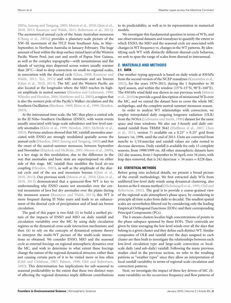
Warm ENSO events (Figure 5A) are dominated by WT 1,followed by a large frequency increase of WT 2 until midDecember. The core of the austral summer monsoon isalmost equally dominated by WT 4 and the largely quies-cent WT 5, which is significantly more frequent than usual.






FIGURE 5 | WT composites in running 31-day windows, classified by (A)

warm, (B) cold and (C) neutral ENSO events. These are defined as themean December–February SST anomalies in the Niño 3.4 box lying above+0.5◦C (warm), below −0.5◦C (cold), and between −0.5◦C and +0.5◦C

(neutral) relative to the 1979/80-2012/13 mean. The dots—large and coloredfor positive and small and black for negative frequency deviations—indicatestatistical significance at the two-sided 95% level as tested by 1000 randompermutations of the observed yearly sequence of WTs.

WT 3 occurs significantly less frequently than expected dur-ing the austral summer monsoon, with always < 15% of days.The cold ENSO events (Figure 5B) are mostly related to anincreased frequency of WT 3, especially around November-December and also in February-April. WT 2, and secondar-ily WT 5, occur less frequently than usual. The correlation

between the September-April averaged Niño 3.4 SST indexand seasonal WT frequency equals 0.34, with p-value = 0.06according to a random-phase test (Janicot et al., 1996), 0.54(p-value < 0.01), −0.76 (p-value < 0.01), 0.16 (p-value = 0.17),0.81 (p-value < 0.01) and −0.57 (p-value < 0.01) for WTs 1–6,respectively.





These results suggest that ENSO strongly modulates both thepersistence and the recurrence of WTs. Moreover, the neutralyears (Figure 5C) do not show large anomalies and the seasonalevolution is then close to the long-term mean—except for, usu-ally short, spells of excess of WT 2 around mid-November andin March-April and WT 4 after mid-November and aroundmid-February.

We next investigate whether there are significant changes inWT pattern during the different ENSO phases. Figure 6 showscomposite WT anomalies for the warm (left column) and cold(middle column) ENSO events identified in the previous para-graphs, while the difference in WT pattern between warm andcold ENSO events is shown in the right column. The 850 hPa

winds (vectors) and OLR anomalies (shading) are expressed asanomalies relative to the total-field composites of each WT shownin Figure 4. These anomaly maps thus express the ENSO effect onchanges in WT pattern and they are plotted in color only whenthey are significant at the two-sided 95% level, according to ourKS test.

Large areas of significant ENSO impacts on WT pattern arevisible, with El Niño tending to decrease convection and La Niñato increase it, broadly across all six WTs. To test globally thehypothesis whether the WTs patterns are significantly modu-lated by ENSO phase, the field significance of these composites isevaluated as follows: in place of the warm and cold years, respec-tively, 10 and 13 years are randomly chosen 1000 times and the

FIGURE 6 | Mean OLR (shading in Wm−2) and 850-hPa wind

anomalies: (left column) 10 warmest ENSO events; (middle column)

13 coldest ENSO events; and (right column) difference between

warm and cold ENSO events for (A–C) WT 1, (D–F) WT 2, (G–I) WT

3, (J–L) WT 4, (M–O) WT 5, (P–R) WT 6. Warm and cold ENSO events

are defined as in Figure 5. The OLR anomalies are shown in color onlywhen they are significant at the two-sided 95% level according to theKolmogorov-Smirnov (KS) test described in Section 3.2. The 850 hPawinds anomalies are plotted as vectors only when zonal or meridionalwinds are significant at the two-sided 95% level according to the KS test.






KS-significant areas are computed for each of the three columnsof Figure 6.

For the composite wind fields, the significant area is neverreached by more than 10% of the random samples, except for thewind of WT 3 (=33% for the zonal and meridional components)in cold ENSO events, and for the wind of WT 5 (=14% for thezonal and =11% for the meridional component), in warm ENSOevents. For OLR, the significant area observed in warm and coldENSO events is never reached by more than 8% of the randomnoise samples.

Our global KS tests thus confirm that the difference betweenWT patterns observed during cold vs. warm ENSO events cannotbe attributed to sampling uncertainty, and that ENSO signifi-cantly modulates the WT patterns, in addition to WT frequency.This systematic modulation (right column of Figure 6) is nearlyconstant across the WTs, with an anomalous regional-scale diver-gence (convergence) at 850 hPa centered between Mindanao, Javaand NW Australia, combined with anomalous subsidence (ascen-dance) over most of the MC, while a small area of enhanced(reduced) convection appears over the equatorial Pacific east ofNew Guinea, during warm (cold) ENSO events.

3.2.2. Sub-seasonal variabilityAt sub-seasonal scales, Figure 7 quantifies the impact on WT fre-quency of phase locking with the eight MJO phases—as definedby Wheeler and Hendon (2004) and used for predictive purposesby Kondrashov et al. (2013). In the upper panel, it is clear that theoccurrence of the active-monsoon WTs 3 and 4 is favored dur-ing MJO phases 5–7, during which convection is enhanced fromIndonesia to the western Tropical Pacific, while WTs 5 and 6—which represent weak, or break, monsoon episodes—occur morefrequently during MJO phases 1–3, associated with enhancedconvection mostly over the Indian Ocean (Wheeler and Hendon,2004).

The anomalous WT frequencies were also computed for the 10warm ENSO and 13 cold ENSO seasons in the middle and lowerpanels of Figure 7. The association between WT frequency andMJO phases is also seen, separately, in El Niño and La Niña years.However, the active-monsoon WTs 3 and 4 are more strongly sup-pressed in MJO phases 1–3 and more strongly favored in MJOphases 4–7 during El Niño episodes (middle panel). Thus, MJOforecasts may be of particular value during El Niño years for earlywarning of drought and flood episodes.

A KS test of significant changes in WT pattern was also per-formed for the 8 MJO phases, analogous to the one describedfor the ENSO phases in Figure 6. However, in the case of MJO,the result of the global field significance test was negative—theobserved significant area is usually beaten by more than 10% ofthe random samples except for respectively 3 and 1 cases outof 48 (=6 WTs × 8 MJO phases) tests in zonal and meridionalwinds—i.e., there is usually no significant perturbation of the WTpatterns by MJO phase.

The above analyses suggest that (1) the annual cycle exertsa strong control on WT occurrence; (2) ENSO events impactthe frequency of WTs (mostly WT 2, 3, 5, and 6) as well astheir patterns, through spatially homogeneous, sustained atmo-spheric anomalies across the MC—i.e., suppressed regional-scale

convection during warm ENSO events—rather than changingthe overall pattern of each WT; while (3) MJO impacts only thefrequency of WTs. The relative impact of each of the three quasi-periodic forcings on WT frequency, and of their combinations, isestimated next, using a multinomial logistic regression.

3.2.3. Predictive models of WT frequency based on seasonal cycle,ENSO and MJO

Our goal here is to retrospectively forecast WT occurrencefrequency, given perfect knowledge of these three regional climatedrivers. We first construct two filtered daily time series to repre-sent the seasonal cycle and Niño 3.4 SSTs, since the 8 MJO phasesare already available from Wheeler and Hendon (2004). The sea-sonal cycle is estimated with the first PC of standardized anoma-lies of the zonal and meridional components of the 850-hPa wind,while keeping the seasonal cycle and analyzing the full year. Thefirst PC is low-pass filtered with a recursive Butterworth filter oforder 9 and with a cut-off = 1/90 cycle-per-day. The variabilityincludes a quasi-regular seasonal cycle combined with a minormodulation at the interannual time scale related with ENSO vari-ability: the correlation between the September–April average ofPC 1 and the Niño 3.4 index is 0.63.

We remove the ENSO-related variance by linear regressionas follows: A daily time series is created from the monthly SSTanomaly of the Niño 3.4 index (NINO hereafter) by first samplingmonthly values at a daily time scale and then filtering this timeseries with the same Butterworth filter as PC1 above. The Niño3.4 effect is then removed from PC1 through linear regressionand the extraction of the residual. The annual index so obtainedis referred to hereafter as AN.

Table 2 shows the seven possible multinomial logistic regres-sion models when using the three distinct predictors AN, NINOand MJO of daily WT occurrence. The “null” model (first rowof the table) takes into account only an independent term andits deviance is analogous to the sum of squared errors in linearregression, providing a baseline for model comparison. All thechanges in the model deviances �G2 between a nested model,i.e., adding one or more predictors, and a parent one, are sta-tistically significant at the one-sided 99.9% level, according to achi-squared test with 5 degrees of freedom (Guanche et al., 2014),where 5 equals the number of added predictors (=1 in our cases),by the number of WTs (= k) minus 1. Hence the addition of thepredictors significantly improves the model fit.

AN provides clearly the largest decrease of deviance, whileMJO and NINO contribute roughly equally to this decrease.Considering the three predictors together improves the fit rela-tive to the best model using two predictors, i.e., AN and NINO(fifth row of the table). In other words, the joint impact of AN,NINO and MJO provides the best fit of the observed sequences ofdaily WTs.

The cross-validated hit rates (rightmost 7 columns of the table)confirm the differential impact of the three predictors on theoccurrence of each WT. NINO (third row in the table) is a majordriver of the occurrence of WT 3 and WT 5 during the wet sea-son, while WT 4 frequency is mostly affected by AN (row 2; cf.Figure 3). The marginal impact of MJO (row 4) is largest forWTs 4 and 5.





FIGURE 7 | Phase locking of the WTs to the 8 phases of the MJO

(Wheeler and Hendon, 2004; Kondrashov et al., 2013) expressed as

anomalous conditional probability of WT occurrence during MJO

phases. The filled orange and blue dots indicate significant positive and

negative anomalies, respectively, at the two-sided 95% level, as tested by1000 random permutations of the observed daily sequences of the WTs. (A)

anomalies computed for all 34 seasons; and (B,C) anomalies discretized forthe warm and cold ENSO events, respectively, defined as in Figure 5.

The joint impact of AN and MJO is rather similar to that ofAN and NINO, except for WT 3, even though the marginal effectsof NINO and MJO (rows 3 and 4) strongly differ, AN being thedominant one. The interannual variability of the WT probability

is well-specified by the model including all three AN, NINO andMJO, with correlations between hindcast and observed seasonalfrequency equal to 0.73 (WT 1), 0.50 (WT 2), 0.78 (WT 3), 0.66(WT 4), 0.83 (WT 5) and 0.58 (WT 6), all values being significant






Table 2 | Fitting diagnostic and cross-validated hit rates for different multinomial logistic models (Gloneck and McCullagh, 1995), including the

three distinct predictors indicated in the first column (see text); the first model (“null”) includes only the intercept and is not cross-validated.

Model G2 �G2 WT 1 WT 2 WT 3 WT 4 WT 5 WT 6 All WTs

(1180 days) (1245 days) (1393 days) (1463 days) (1628 days) (1319 days) (8228 days)

1: Null 2.9362 ×104

2: AN 1.8951 ×104 (vs. 1) 1.0411 ×104 978 260 0 1189 853 725 4005

3: NINO 2.8523 ×104 (vs. 1) 839 0 0 950 7 1136 190 2286

4: MJO 2.8789 ×104 (vs. 1) 573 0 0 0 915 1134 3 2052

5: AN + NINO 1.8005 ×104 (vs. 2) 945 973 364 720 1024 770 729 4580

6: AN + MJO 1.8265 ×104 (vs. 2) 686 1004 386 347 1171 873 695 4476

7: NINO + MJO 2.785 ×104 (vs. 3) 673 0 42 716 492 849 424 2953

8: All 3 1.7273 ×104 (vs. 5) 731 1013 412 751 1042 796 751 4765

The other models are cross-validated with parameters iteratively learned on 33 years and WT probability computed on the remaining year. The change of deviance

�G2 between a model (indicated in parenthesis) and a nested one using additional predictors is always significant at the one-sided 99.9% level, i.e., increasing the

number of predictors is always justified at this level. The last 7 columns show the accuracy of the models, computed as the hit rate of each WT in cross-validation.

The observed and hindcast WT are estimated as the maximum probability amongst the 6 WTs for running 11-day windows centered on each target day. The bold

values show the highest hit rate for each WT.

at the one-sided 95% level according to a random-phase test(Janicot et al., 1996).

3.2.4. Filtering of WT patternsFinally, we compare the interannual and sub-seasonal anomaliesfor each WT, with respect to the mean annual cycle calculated on adaily basis. The goal here is to separate the phenomena associatedwith each WT by filtering the contributions to the compositeWT maps in Figure 4 from the interannual and sub-seasonalfrequency bands. For example, if they were solely a reflectionof ENSO impacts, then applying a high-pass sub-seasonal filterwould yield near-zero anomalies for each WT. This analysis com-plements the previous ones, since we do not assume a priori thespecial role of ENSO or MJO, while the dominant driver of WToccurrence, i.e., the mean seasonal cycle, is filtered out.

The anomalies are computed as deviations between raw val-ues (shown in Figure 4) and the mean seasonal cycle; they arethen decomposed into two additive components, on either sideof a period of 242 days—i.e., the length of the extended australsummer, September 1–April 30—by using a 9th-order recursiveButterworth filter with a cut-off frequency of (1/242) cycle/day.The composites for each of the two frequency bands are thenplotted for each WT in Figure 8. Note that this analysis makes nodistinction between the impacts of the respective oscillation onWT frequency vs. WT amplitude: it merely assesses the relativeroles of ENSO and MJO in giving rise to these WTs.

The pattern correlations between the interannually and sub-seasonally filtered WTs in Table 3 indicate substantial similar-ity in both OLR and wind anomalies, especially for WTs 2,3, and 5. These three WTs are also the most variable intheir frequency of occurrence at the interannual time scale (cf.Table 1).

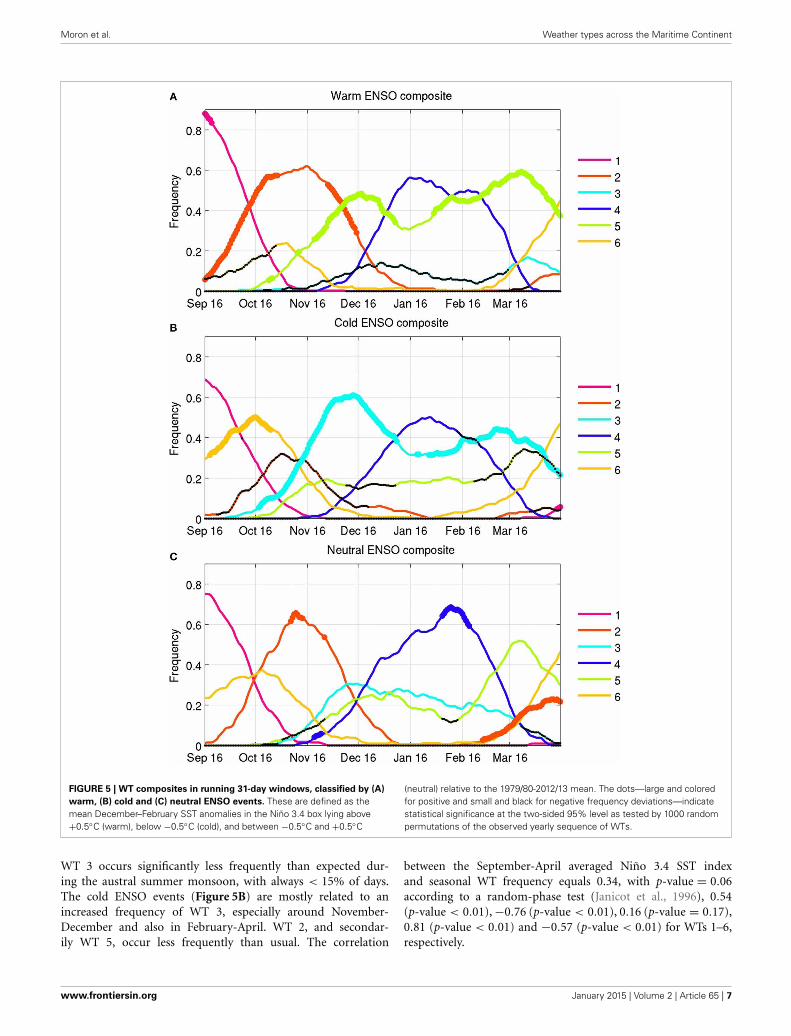
Figure 8 shows that the anomalies are generally stronger in thesub-seasonal than in the interannual band. WT 3 is associatedwith anomalous low-level convergence and enhanced deep con-vection over Central Indonesia, while anomalous subsidence and

therewith positive OLR anomalies, as well as increased low-leveleasterlies are observed over the Western Tropical Pacific. WT 5shows an almost reversed pattern, with anomalous low-leveldivergence centered over New Guinea, accompanied by east-erly anomalies and increased subsidence over most of Indonesia.WT 2 has some similarities with WT 5, except that anomalouslow-level divergence, i.e., higher OLR, occurs between the SouthChina Sea and Northern Australia.

The similarity between sub-seasonal and interannual compo-nents is less obvious for WTs 1, 4, and 6, which also tend to showrather weak interannual components (Table 3); this weaknesssuggests that these WTs do tend to be less excited by interannualforcing, and indeed the interannual variability of their frequencyof occurrence tend to be small, cf. Tables 1, 3.

3.3. WEATHER TYPES: ASSOCIATED LOCAL-SCALE RAINFALLANOMALIES

The analyses so far have focused on regional-scale anomalies.Downscaling to local-scale anomalies is now considered, using the0.25◦ × 0.25◦ TRMM dataset (Huffman et al., 2007). We need tobe cautious about these analyses since they refer to the secondhalf of the period only and there are known biases in the TRMMremote-sensing data relative to in situ rain gages (Dinku et al.,2007).

As before, we decompose the rainfall anomalies according totime scale. This provides a measure of how interannual and sub-seasonal rainfall variability is described by changes in frequencyand amplitude of daily WTs. We first computed interannual andsub-seasonal anomalies in rainfall as in Figure 8, after taking thecubic root of daily rainfall values to reduce skewness.

As for OLR and 850-hPa winds, there is a significant pat-tern correlation between interannual and sub-seasonal anomalies(Table 3). For each WT there is an expected broad-scale inverserelationship between OLR (Figure 8) and rainfall anomalies(Figure 9). However, this association does not hold everywhere,in particular not over islands. The quiescent WT 5, for example,





FIGURE 8 | OLR (shadings in Wm−2) and 850 hPa winds: (left

column) interannual and (right column) sub-seasonal anomalies

associated with (A,B) WT 1, (C,D) WT 2, (E,F) WT 3, (G,H) WT 4, (I,J)

WT 5 and (K,L) WT 6. The significance is computed by using 1000random permutations of non-overlapping blocks of 22 days of daily WT

sequences amongst the 34 years to account for the mean seasonalcycle, i.e., taken at the same stage of the cycle, and shown as color(OLR) and vectors (850-hPa wind) only when OLR, zonal or meridionalcomponents of the wind are above the two-sided 95% level ofsignificance according to random permutations.






Table 3 | Pattern correlation between the interannual and

sub-seasonal anomalies associated with each WT shown in Figure 6.

U 850 hPa V 850 hPa OLR TRMM rainfall

WT 1 0.32 0.03 0.46** 0.34**

WT 2 0.82** 0.55** 0.73** 0.63**

WT 3 0.82** 0.75** 0.76** 0.62**

WT 4 0.26 0.43* 0.22 0.23

WT 5 0.83** 0.81** 0.49** 0.38**

WT 6 0.60** 0.57** 0.54** 0.39**

One and two asterisks indicate significant values at the one-sided 95% and 99%

level, respectively, according to a random permutation of non-overlapping blocks

of 22 days of daily sequences amongst the 34 years (15 years for rainfall) to

account for the mean seasonal cycle.

is associated at sub-seasonal scales (Figure 8) with positiveOLR anomalies—almost everywhere, except over the easternIndian Ocean—but positive rainfall anomalies are observed overSumatra, western Borneo, Java, and Sulawesi, especially at sub-seasonal scales (Figure 9). Note also that dipolar precipitationanomalies appear over Borneo and New Guinea, especially forWTs 3, 5, and 6. The positive rainfall anomalies tend to be locatedin the lee of the mountains, in particular along the northwestcoast of Borneo and in central New Guinea. This “island wake”effect (Qian et al., 2013) may be associated with land-sea breezeenhancement on the mountains’ lee side.

The relationship between OLR and small-scale rainfall anoma-lies is further investigated in Figure 10. OLR is first interpolatedonto the much finer TRMM grid over the same time interval,from 1998/99 on, as daily rainfall. The anomalies relative to themean seasonal cycle of daily means are then standardized to zeromean and unit variance and spatially averaged for the core regionof the MC (94◦E–125◦E, 10◦S–6◦N).

At this regional scale (Figure 10A), there is a broad anti-symmetry between OLR and rainfall anomalies, even thoughrainfall anomalies are closer to zero. Considering only the islandpoints (Figure 10B) tends to weaken this anti-symmetry forWTs 2 and 3, where median rainfall anomalies tend to zero, andespecially so for WT 5; in WT 5, OLR and rainfall anomaliesare both positive, thus associating suppressed regional-scale deepconvection with positive local-scale rainfall anomalies that couldnot be accurately captured by the OLR field’s spatial resolution inour data. Such specifically asymmetric behavior of WT 5 appearsalso at even smaller scales, as seen over Java in Figure 10C.

3.4. WEATHER TYPES: VARIATIONS IN THE DIURNAL CYCLEDiurnal-cycle variations are systematically analyzed for our sixWTs by considering the 3-hourly mean rainfall at each grid pointthat corresponds to the climatological peak phase of the diurnalcycle; this peak occurs in the late afternoon to early night overislands and late night to early morning around islands, with noclear peak observed over open seas. The rainfall for the diurnalpeak is standardized with respect to the mean seasonal cycleand averaged for each of our six WTs; the results are plotted inFigure 11.

The local-scale significance is estimated using the same per-mutation method as the one employed for Figure 9. The peakphase of the diurnal cycle is enhanced with respect to clima-tology over Java in WT 5, as expected, but also over most ofSumatra, southwest Borneo, Sulawesi, and most of the Sundaislands (Figure 11E), while peak daily rainfall is significantlybelow climatology over most of the open seas, except off thewestern coasts of Sumatra and Borneo.

The positive rainfall anomalies over islands east of 105◦E inWT 5 are not related to enhanced large-scale convection, butrather to the increased strength of the diurnal cycle at small spa-tial scales, when eastward anomalies are superimposed on thenormal westerlies associated with the austral summer monsoon(Moron et al., 2010; Qian et al., 2010, 2013), as well as tolocal-scale SSTs (Hendon, 2003; Qian et al., 2013). This spe-cial phenomenon for the “quiescent” WT 5 may be explained bythe inverse relationship between the monsoonal wind speed andthe intensity of diurnal cycle, increasing sea-breeze and valley-breeze convergence toward the mountains during weak monsoon,thus brings forth more rainfall over the mountains than over theadjacent plains and seas (Moron et al., 2010; Qian et al., 2010).

4. CONCLUDING REMARKS4.1. SUMMARYIn this paper we have analyzed the characteristics of atmosphericvariations over the Maritime Continent (MC) using the pat-tern recognition framework of weather typing. This frameworkhas been extensively used for the extratropics (Mo and Ghil,1988; Vautard and Legras, 1988; Kimoto, 1989; Vautard, 1990;Michelangeli et al., 1995; Ghil and Robertson, 2002) but less soin the tropics.

The MC shows a rich spectrum of temporal variations(Figure 2), including a strong seasonal cycle associated with themigration of the planetary-scale ITCZ. Our study focused on theaustral summer monsoon, 1 September–30 April, for 34 seasonsfrom 1979/80 to 2012/13. Six weather types (WTs) were obtainedusing k-means cluster analysis of unfiltered daily low-level windfields (Figures 3, 4).

We interpreted these six WTs firstly as stages of the sea-sonal progression of the planetary-scale monsoon circulation(Figure 3) from the pre-monsoonal WT 1 through the core mon-soonal WTs 3–5 and on to the post-monsoonal WT 6. Thepre-monsoonal WT 1 and transitional WTs 2 are thus charac-terized by the low-level easterlies south of the equator that arecommon to both pre- and post-monsoonal stages.

Values of OLR below 210 Wm−2 are restricted to the northof the equator in WT 1 and shifted toward two near-equatorialminima, between Sumatra and Borneo, on the one hand, andbetween New Guinea and the Western Tropical Pacific, on theother, in WTs 2 and 6 (Figure 4). Marked seasonal changes takeplace in November–March, with a progression toward the mon-soonal WTs 3–5 accompanied by westerlies that are strongestin WT 4, but quiescent in WT 5, and the strongest deep con-vection occurring south of the equator. WT 4 corresponds tothe peak of the austral summer monsoon with strong westerliesreaching Northern Australia and a clear equatorial westerly flowfrom Sumatra to the Western Pacific (Figure 4).





FIGURE 9 | Same as Figure 8, except for daily rainfall from the TRMM

3b42 (version 7) dataset (Huffman et al., 2007). Rainfall data are availablefrom 1998/1999 on only. Daily rainfall (in 1/10 mm/day) are cube rooted

before the computation of climatological mean and anomalies. Thesignificance is computed as in Figure 8, except that only 15 years areavailable for the randomizing of the sequences.






FIGURE 10 | OLR (black) and TRMM rainfall (red) standardized

anomalies relative to the mean seasonal cycle for each WT, from

1998/1999 on only. Daily rainfall values (in 1/10 mm/day) are cube-rootedbefore the computation of climatological mean and anomalies;

median—central horizontal line, upper and lower quartiles—upper andlower limits of the box. (A) Whole MC core area; (B) islands only; and (C)

Java only. The plot for the sea only (not shown) is practicallyindistindinguishable from panel (A). See text for details.

Using the WT framework, interannual and sub-seasonal vari-ations lend themselves to interpretation in terms of changes inWT frequency of occurrence and their associated atmosphericanomalies at these scales (Figures 5–8). On the interannual timescale, the strongest anomalies are observed for WT 3, on theone hand, and WT 2 and 5, on the other: WT 3 (respectivelyWT 2 and 5) exhibits low-level anomalous convergence (respec-tively divergence) over eastern and/or central MC, along withenhanced (respectively suppressed) regional-scale deep convec-tion (Figure 8). The interannual signal is weaker for the pre- andpost-monsoon WTs 1 and 6, as well as for the peak WT 4 of theaustral summer monsoon.

This behavior is consistent with the anomalies in WT fre-quency observed during ENSO events. Warm ENSO eventsare mostly associated with an increased occurrence of WT 1,

followed by WT 2—which delays the regional-scale onset ofthe austral summer monsoon—and then by an increased fre-quency of the quiescent WT 5 during the rainy season; thelatter corresponds to a superimposition of low-level easterlyanomalies (Figure 6) upon the climatological westerlies asso-ciated with the austral summer monsoon (Figure 4). WTs 2and 5 are associated with an enhanced diurnal cycle in thenorthern and southern MC, respectively, where synoptic windsare weak; weak winds lead to positive rainfall anomalies oversome islands, or parts of islands, while large-scale subsidencepromotes negative rainfall over most of the MC’s inner seas(Figure 11). These results are consistent with our previous work(Moron et al., 2009, 2010; Qian et al., 2010, 2013), as well aswith (Jourdain et al., 2013), who found that the anti-correlationbetween MC precipitation and the Niño 3.4 index in DJFM is





FIGURE 11 | TRMM rainfall anomalies (shadings) for the peak of the

diurnal cycle at each grid point and raw 850-hPa daily winds

(vectors) for (A) WT 1, (B) WT 2, (C) WT 3, (D) WT 4, (E) WT 5, (F)

WT 6. The TRMM anomalies are computed as the differences from the

climatological daily mean. Maximum daily rainfall values (in 1/10 mm/day)are cube-rooted before the computation of climatological mean andanomalies. The significance is computed and plotted as in Figure 9; seetext for details.

more marked over ocean than over land in CMIP3 and CMIP5model runs.

Cold ENSO events are not exactly symmetric, with more WT 6episodes occurring just before the austral summer monsoon andespecially more WT 3 than usual during the core of the rainyseason. ENSO events do also modify the spatial pattern of WTsthrough the superposition of persistent anomalies associated withregional-scale anomalous subsidence (ascendance) during warm(cold) ENSO events (Figure 6).

On sub-seasonal time scales, the variation of WT frequen-cies is partly attributable to the MJO, with WTs 3–6 significantlylocked with MJO phases. The sub-seasonal circulation anoma-lies are more pronounced amongst the WTs (Figure 8) but aresimilar to those on interannual time scales in their patterns, espe-cially for WTs 2, 3, and 5. However, contrary to the effect ofENSO events, MJO does not appear to impact the WT patternsthemselves significantly.

4.2. DISCUSSIONOur results show that the WT framework can provide flexi-ble tools to diagnose atmospheric anomalies across time scales,

analyze potential predictability, and provide an easy way to spa-tially downscale any variable related to WT occurrence. Weathertyping applied to unfiltered daily values covers in theory all timescales—from daily to interannual and interdecadal—i.e., up tothe total number of years included in the analysis, equal here to34 years. Of course, using EOF pre-filtering prior to the k-meansclustering filters out the smallest and fastest variations. The reduc-tion to a small set of WTs, equal here to six for 8228 days, also actsas a filter, while other clustering techniques (e.g., self-organizingmaps) usually consider a larger set of situations, often more than16, e.g., (Verdon-Kidd and Klem, 2009; Brown et al., 2010).

In any clustering, there is a trade-off between robustness andresolution. Transient mesoscale and synoptic-scale features, likethe Borneo vortex (e.g., Chang et al., 2003, 2005b; Tangang et al.,2008) or individual tropical depressions or even cyclones (Changet al., 2003) are obviously not captured by a small number of WTs,but this does not mean that WTs do not provide information onfast and small scales. As soon as one WT is associated with sys-tematic and reproducible variations at any scale, this informationis retrievable in the WT framework. It is the case here with thesystematic modulation of the diurnal cycle over several islands






or parts thereof—including Sumatra, western Borneo, Java, andSulawesi—mostly in WT 5 and, at least, in sectors where a com-bination of sub-seasonal to seasonal variations and the annualcycle weakens the regional-scale winds and thus increases thediurnal-cycle amplitude (Moron et al., 2010; Qian et al., 2013).

In their recent study, Peatman et al. (2013) concluded that80% of the MJO precipitation signal over the MC is accountedfor by changes in the amplitude of the diurnal cycle, whichresponds over islands about 6 days in advance of the arrival ofthe main MJO convective envelope. They argue that frictionaland topographic moisture convergence and relatively clear skiesthen combine with the low thermal inertia of the islands, to allowa rapid response in the diurnal cycle. According to our results,the “quiescent” WT 5 is responsible for the strong diurnal signalover islands, and it is most prevalent in MJO phases 1–3, whenthe MJO convective envelope is over the Indian Ocean (Figure 7).We argue that the quiescent large-scale winds of WT 5 allow thediurnal cycle to amplify, as described in Qian et al. (2010, 2013).

Although the MJO modulation of WT 5 is most marked dur-ing La Niña events (Figure 7C), this is tempered by the muchless frequent occurrence of WT 5 during the cold phase of ENSO(Figure 5B), so that this MJO modulation of diurnal precipitationis less likely to be observed at that time.

An early dynamical interpretation of extratropical WTs,or planetary flow regimes (Legras and Ghil, 1985; Ghil andChildress, 1987), was in terms of fixed points of the governingflow equations. In the tropics, moist processes play a larger rolethan in mid-latitudes, and one can thus expect the need for morecomplex interpretations. Moreover, boundary forcing by SSTs inthe tropics is much more important than in mid-latitudes. In par-ticular, we found here that WTs can capture transient modes orsystematic variations, such as the seasonal cycle. We have shown,in fact, that WTs can be interpreted, to first order, as fixed snap-shots of the annual cycle, since this time scale was retained in ouranalysis and not filtered out at the outset, as is typically done.

Furthermore, it was possible to separate the atmosphericanomalies associated with each WT according to large-scale cli-mate phenomena on both the interannual and sub-seasonal scale,namely as being affected by either ENSO or the MJO, respec-tively. For example, the broad-scale easterly anomalies observedin WTs 2 and 5 refer clearly to warm ENSO events, acting throughlarge-scale subsidence over eastern Indonesia. Likewise we foundthat WT 5 is more phase-locked to MJO than WT 2 is. Sucha data-adaptive, WT-mediated decomposition of time scales iscomplementary to the usual a priori selection that is provided byremoving the mean annual cycle or by bandpass filtering. Our WTframework helps one also to interpret the phase shifts associatedwith the seasonal cycle as the delayed onset of the austral sum-mer monsoon during warm ENSO events, an aspect that may beblurred when the seasonal cycle is filtered out a priori.

Returning to the conceptual framework of dynamical systemstheory introduced in Section 1, we may conclude that the impor-tance of “external” forcings—i.e., of ENSO, the MJO and theseasonal cycle—in the Tropics in general and in the regionaldynamics of the MC in particular—requires the application of thebroader and more flexible concepts of open, non-autonomous,and possibly random dynamical systems (cf. Ghil et al., 2008;

Chekroun et al., 2011; Ghil, 2014) and references therein, whilethe more standard theory of closed, autonomous systems waslargely sufficient for planetary-scale, extratropical phenomena(Ghil and Childress, 1987, Ch. 5). Thus, the seasonal cycle intro-duces a strong periodic modulation of the atmosphere’s dynam-ical attractor over the MC, for which the six discrete WTs thatoccur in overlapping fashion at different stages of the monsoonalprogression provide a robust “skeleton.” For the sake of brevity,we will not enter into the technical aspects of the time-dependentpullback attractors that are required to describe the behavior ofnon-autonomous systems, and only use the concepts loosely inorder to interpret the present findings.

The occurrence frequency of certain WTs is significantlyimpacted from year to year by ENSO and sub-seasonally by theMJO, modulating in time the size and shape of the correspondingattractor basins. Sub-seasonal to seasonal predictability of circula-tion over the MC may be partially framed in terms of the strengthof these frequency modulations. In addition, ENSO was shown toexert an influence on the spatial structure of circulation patternsfor certain WTs, thereby modulating, on interannual time scales,the position that the pullback attractor’s successive “snapshots”occupy in the system’s phase space. This effect is not found for theMJO, whose impact appears to be purely on the WTs’ frequencyof occurrence.

The atmospheric Southern Oscillation limb of ENSO modu-lates the strength of the planetary-scale Walker Circulation, whoseascending branch is located over the MC. Thus, it is very plausi-ble that ENSO would modulate the structure of the MC’s pullbackattractor on shorter spatial scales. While the MJO also has a largewavenumber-one component zonally, it is transient on the timescale of WT transitions and propagates through the MC; it istherefore to be expected that its impact on the WTs would belargely by modulating their frequency, with less impact on theoverall attractor structure.

Besides the theoretical considerations above, the connectionbetween daily weather conditions and large-scale climate driversafforded by the WT framework is very useful from the appliedclimate perspective. For example, farmers in Western Java planttheir first rice crop after monsoon onset in October–December,followed by a second crop, which they plant in May-June. Thefirst is vulnerable to flooding in January-February, and the secondto drought, especially if the monsoon onset is delayed by El Niño(Boer and Subbiah, 2005; Moron et al., 2009). The work presentedhere could help identify the atmospheric drivers of flood anddrought events at local scale within specific WT daily sequences,which in turn may help develop sub-seasonal to seasonal fore-casts that are more accurate and better tailored to the needs offarmers.

ACKNOWLEDGEMENTWe thank F. Kucharski, F. Molteni, J. Shukla, and D. Strausfor their valuable comments and suggestions on the prelimi-nary stages of this paper, during the school and workshop on“Weather regimes and weather types in the tropics and extra-tropics: Theory and application to prediction of weather andclimate” held in October 2013 at the International Centre forTheoretical Physics in Trieste. Three-hourly data from the TRMM





3b42 mission, version 7, have been downloaded free of chargefrom the map room site of the International Research Institute forClimate and Society (IRI; http://ingrid.ldgo.columbia.edu), whileReanalysis-2 and OLR daily data were downloaded free of chargefrom the Earth System Research Laboratory of NOAA’s PhysicalScience Division (http://www.esrl.noaa.gov/psd/data/gridded/).Michael Ghil and Andrew W. Robertson were supported by MURIgrant N00014-12-1-0911 from the Office of Naval Research,and Andrew W. Robertson also by the International Fund forAgricultural Development.

REFERENCESBjerknes, J. (1969). Atmospheric teleconnections from the equa-

torial Pacific. Mon. Wea. Rev. 97, 163–172. doi: 10.1175/1520-0493(1969)097<0163:ATFTEP>2.3.CO;2

Boer, R., and Subbiah, A. R. (2005). “Agricultural droughts in Indonesia,” inMonitoring and Predicting Agricultural Drought: A Global Study, eds V. S. Boken,A. P. Cracknell, and R. L. Heathcote (New York, NY: Oxford University Press),330–344.

Brown, J. R., Jakob, C., and Haynes, J. M. (2010). An evaluation of rainfall frequencyand intensity over the Australian region in a global climate model. J. Clim. 23,6504–6525. doi: 10.1175/2010JCLI3571.1

Chang, C.-P., Liu, C.-H., and Kuo, H.-C. (2003). Typhoon Vamei: an equato-rial tropical cyclone formation. Geophys. Res. Lett. 30. doi: 10.1029/2002GL016365

Chang, C.-P., Harr, P. A., and Chen, H.-J. (2005b). Synoptic disturbances overthe equatorial Souttime Continent during boreal winter. Mon. Wea. Rev. 133,489–503. doi: 10.1175/MWR-2868.1

Chang, C.-P., Wang, Z., McBride, J., and Liu, C.-H. (2005a). Annual cycle ofSoutheast Asia Maritime Continent rainfall and the asymmetric monsoontransition. J. Clim. 18, 287–301. doi: 10.1175/JCLI-3257.1

Chekroun, M. D., Simonnet, E., and Ghil, M. (2011). Stochastic climate dynam-ics: random attractors and time-dependent invariant measures. Physica D 240,1685–1700. doi :10.1016/j.physd.2011.06.005.

Chen, Y., Ebert, E. E., Walsh, K. J. E., and Davidson, N. E. (2013).Evaluation of TRMM 3B42 precipitation estimates of tropical cyclone rain-fall using PACRAIN data. J. Geophys. Res. 118, 1–13. doi: 10.1002/jgrd.50250

Diday, E., and Simon, J. C. (1976). “Clustering analysis,” in Digital PatternRecognition, Communication and Cybernetics, Vol. 10, ed K.S. Fu (Springer-Verlag), 47–94.

Dinku, T., Ceccato, P., Grover-Kopec, E., Lemina, M., Connor, S. J., andRopelewski, C. F. (2007). Validation of satellite rainfall products over EastAfrica’s complex topography. Int. J. Remote Sensing 28, 1503–1526. doi:10.1080/01431160600954688

Ghil, M. (2014). “A mathematical theory of climate sensitivity or, How to dealwith both anthropogenic forcing and natural variability?,” in Climate Change:Multidecadal and Beyond, eds C. P. Chang, M. Ghil, M. Latif, and J. M. Wallace(London: World Scientific Publishing Co.; Imperial College Press).

Ghil, M., and Childress, S. (1987). Topics in Geophysical Fluid Dynamics:Atmospheric Dynamics, Dynamo Theory and Climate Dynamics.New York; Berlin; Tokyo: Springer-Verlag. doi: 10.1007/978-1-4612-1052-8

Ghil, M., and Robertson, A. W. (2002). “Waves” vs. “particles” in the atmosphere’sphase space : a pathway to long-range forecasting? Proc. Natl. Acad. Sci. U.S.A.99, 2493–2500. doi: 10.1073/pnas.012580899

Ghil, M., Chekroun, M. D., and Simonnet, E. (2008). Climate dynamics andfluid mechanics: natural variability and related uncertainties. Physica D 237,2111–2126. doi: 10.1016/j.physd.2008.03.036

Gloneck, G. F. V., and McCullagh, P. (1995). Multivariate logistic models. J. R. Stat.Soc. Ser. B 57, 533–546.

Guanche, Y., Minguez, R., and Méndez, F. J. (2014). Autoregressive logistic regres-sion applied to atmospheric circulation patterns. Clim. Dyn. 42, 537–552. doi:10.1007/s003 82-013-1690-3

Haylock, M., and McBride, J. L. (2001). Spatial coherence and predictability ofIndonesian wet season rainfall. J. Clim. 14, 3882–3887. doi: 10.1175/1520-0442(2001)014<3882:SCAPOI>2.0.CO;2

Hendon, H. H. (2003) Indonesian rainfall variability: impacts of ENSOand local air-sea interaction. J. Clim. 16, 1775–1790. doi: 10.1175/1520-0442(2003)016<1775:IRVIOE>2.0.CO;2

Hendon, H. H., and Liebmann, B. (1990). The intraseasonal (30–50 day) oscil-lation of the Australian summer monsoon. J. Atmos. Sci. 47, 2909–2923. doi:10.1175/1520-0469(1990)047<2909:TIDOOT>2.0.CO;2

Huffman, G. J., Adler, R. F., Bolvin, D. T., Gu, G., Nelkin, E. J., Bowman, K. P., et al.(2007). The TRMM multi-satellite precipitation analysis: Quasi-global, multi-year, combined-sensor precipitation estimates at fine scale. J. Hydrometeor. 8,38–55. doi: 10.1175/JHM560.1

Janicot, S., Moron, V., and Fontaine, B. (1996). Sahel drought and ENSO dynamics.Geophys. Res. Lett. 23, 515–518.

Jourdain, N. C., Sen Gupta, A, Taschetto, A. S., Ummenhofer, C. C., Moise, A.F., and Ashok, K. (2013). The Indo-Australia monsoon and its relationship toENSO and IOD in reanalysis data and the CMIP3/CMIP5 simulations. Clim.Dyn. 41, 3073–3102. doi: 10.1007/s00382-013-1676-1

Juneng, L., and Tangang, F. (2005). Evolution of ENSO-related rainfall anomaliesin SouthEast Asia region and its relationship with atmosphere-ocean variationsin the Indo-Pacific sector. Clim. Dyn. 25, 337–350. doi: 10.1007/s00382-005-0031-6

Kanamitsu, M., Ebisuzaki, W., Woollen, J., Yang, S.-K., Hnilo, J. J., Fiorino, M.,et al. (2002). NCEP-DOE AMIP-II Reanalysis (R-2). Bull. Amer. Meteor. Soc. 79,1631-1643. doi: 10.1175/BAMS-83-11-1631

Kimoto, M. (1989). Multiple Flow Regimes in the Northern Hemisphere Winter.Ph.D. thesis, University of California, Los Angeles.

Klein, S. A., Soden, B. J., and Lau, N.-C. (1999). Remote sea surface temperaturevariations during ENSO: evidence for a tropical atmospheric bridge. J. Clim. 12,917–932. doi: 10.1175/1520-0442(1999)012<0917:RSSTVD>2.0.CO;2

Kondrashov, D., Chekroun, M. D., Robertson, A. W. and Ghil, M. (2013). Low-order stochastic model and “past-noise forecasting” of the Madden-Julianoscillation. Geophys. Res. Lett. 40, 5305–5310. doi: 10.1002/grl.50991

Lefèvre, J., Marchesiello, P., Jourdain, N. C., Menkes, C., and Leroy, A. (2010).Weather regimes and orographic circulation. Marine Poll. Bull. 61, 413–431. doi:10.1016/j.marpolbul.2010.06.012

Legras, B., and Ghil, M. (1985). Persistent anomalies, blocking and variations inatmospheric predictability. J. Atmos. Sci. 42, 433–471.

Liebmann, B., and Smith, C. A. (1996). Description of a complete (inter-polated) outgoing longwave radiation dataset. Bull. Amer. Meteor. Soc. 77,1275–1277.

Livezey, R. E., and Chen, W. Y. (1983). Statistical field significance and its determi-nation by Monte Carlo techniques. Mon. Wea. Rev. 111, 46–59.

Madden, R. A., and Julian, P. R. (1971). Detection of a 40-50 day oscillation in thezonal wind in the Tropical Pacific. J. Atmos. Sci. 28, 702–708. doi: 10.1175/1520-0469(1971)028<0702:DOADOI>2.0.CO;2

Matthews, A. J., and Li, H.-Y.-Y. (2005). Modulation of station rainfall over theWestern Pacific by the Madden-Julian oscillation. Geophys. Res. Lett. 32, L14827.doi: 10.1029/2005GL023595

McBride, J. L., Haylock, M. R., and Nicholls, N. (2003). Relationshipsbetween the Maritime Continent heat source and the El Niño SouthernOscillation phenomenon. J. Clim. 16, 2905–2914. doi: 10.1175/1520-0442(2003)016<2905:RBTMCH>2.0.CO;2

Michelangeli, R. A., Vautard, R., and Legras, B. (1995). Weather regimes: recur-rence and quasi-stationarity. J. Atmos. Sci. 52, 1237–1256. doi: 10.1175/1520-0469(1995)052<1237:WRRAQS>2.0.CO;2

Mo, K., and Ghil, M. (1988). Cluster analysis of multiple planetary flow regimes. J.Geophys. Res. 93, 927–952. doi: 10.1029/JD093iD09p10927

Moron, V., Robertson, A. W., and Qian, J.-H. (2010). Local versus regional-scalecharacteristics of monsoon onset and post-onset rainfall over Indonesia. Clim.Dyn. 34, 281–299. doi: 10.1007/s00382-009-0547-2

Moron, V., Robertson, A. W., and Boer, R. (2009). Spatial coherence and sea-sonal predictability of monsoon onset over Indonesia. J. Clim. 22, 840–850. doi:10.1175/2008JCLI2435.1

Moron, V., Robertson, A. W., and Ghil, M. (2012). Impact of the modulated annualcycle and intraseasonal oscillation on daily-to-interannual rainfall variabilityacross monsoonal India. Clim. Dyn. 38, 2409–2435. doi: 10.1007/s00382-011-1253-4

Moron, V., Robertson, A. W., Ward, M. N., and Ndiaye, O. (2008). Weather typesand rainfall over Senegal. Part I: observational analysis. J. Clim. 21, 266–287.doi: 10.1175/2007JCLI1601.1


http://ingrid.ldgo.columbia.edu

http://www.esrl.noaa.gov/psd/data/gridded/





Palmer, T. N. (1998). Nonlinear dynamics and climate change: Rossbyslegacy. Bull. Amer. Meteor. Soc. 79, 1411–1423. doi: 10.1175/1520-0477(1998)079<1411:NDACCR>2.0.CO;2

Peatman, S. C., Matthews, A. J., and Stevens, D. P. (2013). Propagation of theMadden–Julian Oscillation through the Maritime Continent and scale inter-action with the diurnal cycle of precipitation. Quart. J. R. Meteorol. Soc. 140,814–825. doi: 10.1002/qj.2161

Pohl, B., Camberlin, P., and Roucou, P. (2005). Typology of pentad circulationanomalies over the Eastern Africa – Western Indian ocean region, and theirrelationship with rainfall. Clim. Res. 29, 111–127. doi: 10.3354/cr029111

Qian, J.-H. (2008). Why precipitation is mostly concentrated over islands in theMaritime Continent. J. Atmos. Sci. 65, 1428–1441. doi: 10.1175/2007JAS2422.1

Qian, J.-H., Robertson, A. W., and Moron, V. (2010). Multi-scale interactionbetween ENSO, monsoon and diurnal cycle over Java, Indonesia. J. Atmos. Sci.67, 3509–3523. doi: 10.1175/2010JAS3348.1

Qian, J.-H., Robertson, A. W., and Moron, V. (2013). Diurnal cycle in weatherregimes and rainfall variability over Borneo associated with ENSO. J. Clim. 26,1772–1790. doi: 10.1175/JCLI-D-12-00178.1

Rauniyar, S. P., and Walsh, K. J. E. (2011). Scale interaction of the diurnal cycleof rainfall over the Maritime Continent and Australia: influence of the MJO. J.Clim. 24, 325–348. doi: 10.1175/2010JCLI3673.1

Robertson, A. W., Moron, V., Qian, J.-H., Chang, C.-P., Tangang, F., Aldrian,E., et al. (2011). “The maritime continent monsoon,” in The Global MonsoonSystem: Research and Forecast, 2nd Edn., eds C.-P. Chang, Y. Ding, G. N.-C.Lau, R. H. Johnson, B. Wang, and T. Yasunari (New Jersey: World ScientificPublishing Co.), 85–97. doi: 10.1142/9789814343411_0006

Tangang, F., Juneng, L., Salimun, E., Vinayachandran, P. N., Seng, Y. K., Reason, C.J. C., et al. (2008). On the roles of the northeast cold surge, the Borneo vortex,the Madden-Julian oscillation and the Indian ocean dipole during the extreme2006/2007 flood in southern Peninsular Malaysia. Geophys. Res. Lett. 35. doi:10.1029/2008GL033429

Teo, C.-K., Koh, T. Y., Lo, J. C.-F., and Bhatt, B. C. (2011). Principal componentanalysis of observed and modeled diurnal rainfall in the Maritime Continent. J.Clim. 24, 4662–4675. doi: 10.1175/2011JCLI4047.1

Vautard, R., and Legras, B. (1988). On the source of midlatitude low-frequencyvariability. Part II: nonlinear equilibration of weather regimes. J. Atmos. Sci. 45,2845–2867. doi: 10.1175/1520-0469(1988)045<2845:OTSOML>2.0.CO;2

Vautard, R., Mo, K. C., and Ghil, M. (1990). Statistical significance testfor transition matrices of atmospheric Markov chains. J. Atmos. Sci. 47,1926–1931.

Vautard, R. (1990). Multiple weather regimes over the North Atlantic: analysis ofprecursors and successors. Mon. Wea. Rev. 118, 2056–2081. doi: 10.1175/1520-0493(1990)118<2056:MWROTN>2.0.CO;2

Verdon-Kidd, D. C., and Klem, A. S. (2009). On the relationship between large-scale climate modes and regional synoptic patterns that drive Victorian rainfall.Hydrol. Earth Syst. Sci. 13, 467–479. doi: 10.5194/hess-13-467-2009

Wheeler, M. C., and Hendon, H. H. (2004). An all-season real-timemultivariate MJO index: development of an index for monitoringand prediction. Mon. Wea. Rev. 132, 1917–1932. doi: 10.1175/1520-0493(2004)132<1917:AARMMI>2.0.CO;2

Conflict of Interest Statement: The authors declare that the research was con-ducted in the absence of any commercial or financial relationships that could beconstrued as a potential conflict of interest.

Received: 01 October 2014; accepted: 12 December 2014; published online: 13 January2015.Citation: Moron V, Robertson AW, Qian J-H and Ghil M (2015) Weather types acrossthe Maritime Continent: from the diurnal cycle to interannual variations. Front.Environ. Sci. 2:65. doi: 10.3389/fenvs.2014.00065This article was submitted to Atmospheric Science, a section of the journal Frontiers inEnvironmental Science.Copyright © 2015 Moron, Robertson, Qian and Ghil. This is an open-access articledistributed under the terms of the Creative Commons Attribution License (CC BY).The use, distribution or reproduction in other forums is permitted, provided theoriginal author(s) or licensor are credited and that the original publication in thisjournal is cited, in accordance with accepted academic practice. No use, distribution orreproduction is permitted which does not comply with these terms.


http://dx.doi.org/10.3389/fenvs.2014.00065










Weather types across the Maritime Continent: from the ...

Documents

Transcript of Weather types across the Maritime Continent: from the ...