Weather routing using dynamic programming to win...

Weather routing – using dynamic programming to win sailing races

OSE SEMINAR 2013

Mikael Nyberg

CENTER OF EXCELLENCE IN

OPTIMIZATION AND SYSTEMS ENGINEERING

AT ÅBO AKADEMI UNIVERSITY

ÅBO NOVEMBER 15 2013

2

Table of Content

Introduction

Weather routing

Dynamic Programming

Weather models

Performance data

Weather routing optimization

Mathematical model

Complexity

“Optimal” routing

Limitations

Conclusions

Mikael Nyberg: Weather routing – using dynamic programming to win sailing races

2|16 Agenda

Weather routing

3|16 Introduction: Weather routing


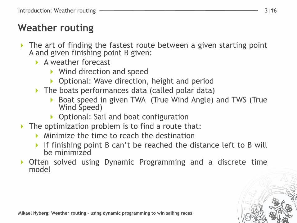
The art of finding the fastest route between a given starting point A and given finishing point B given:

A weather forecast

Wind direction and speed

Optional: Wave direction, height and period

The boats performances data (called polar data)

Boat speed in given TWA (True Wind Angle) and TWS (True Wind Speed)

Optional: Sail and boat configuration

The optimization problem is to find a route that:

Minimize the time to reach the destination

If finishing point B can’t be reached the distance left to B will be minimized

Often solved using Dynamic Programming and a discrete time model

Dynamic Programming

4|16 Introduction: Dynamic Programming


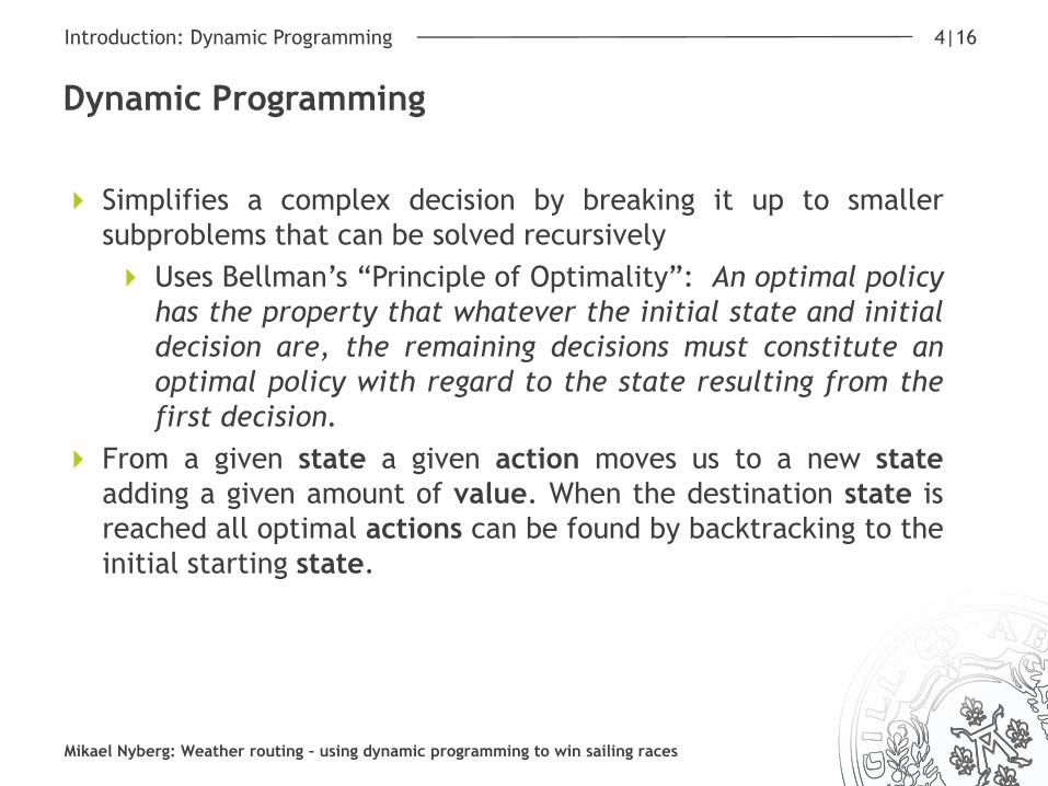
Simplifies a complex decision by breaking it up to smaller

subproblems that can be solved recursively

Uses Bellman’s “Principle of Optimality”: An optimal policy

has the property that whatever the initial state and initial

decision are, the remaining decisions must constitute an

optimal policy with regard to the state resulting from the

first decision.

From a given state a given action moves us to a new state

adding a given amount of value. When the destination state is

reached all optimal actions can be found by backtracking to the

initial starting state.

5

Weather models

For useful and reliable routing good forecasts are needed

Todays’ forecasts are reasonably good up to 7-10 days ahead

Forecasts are distributed in GRIB-files (GRIdded Binary)

Discretization in space: 0.5-1°

Discretization in time: 1-12 hours

For each point in space and time:

TWS (True Wind Speed)

TWD (True Wind Direction)

Pressure

Rain

Forecast for the whole world for 7 days with maximum detail (0.5° and 3 hour resolution and all weather data) ~104 Mb

7 day forecast for the whole world with good detail (1° and 12 hour resolution and TWS, TWD and pressure) ~5.2 Mb


5|16 Introduction: Weather models

6

Polars

The other data set needed for weather routing

is boat performance data - the polars

Gives target boat speeds for given wind

conditions (TWS, TWA)

TWA (True Wind Angle) is the angle

difference between the boat’s heading

and the TWD (True Wind Direction)

Often includes optimal sail plan and boat

configuration to achieve the target speeds

For human use the data is often display as a

polar graph


6|16 Introduction: Performance data

Polar graph for a Beneteau Figaro

7

Weather routing optimization


7|16 Weather routing optimization

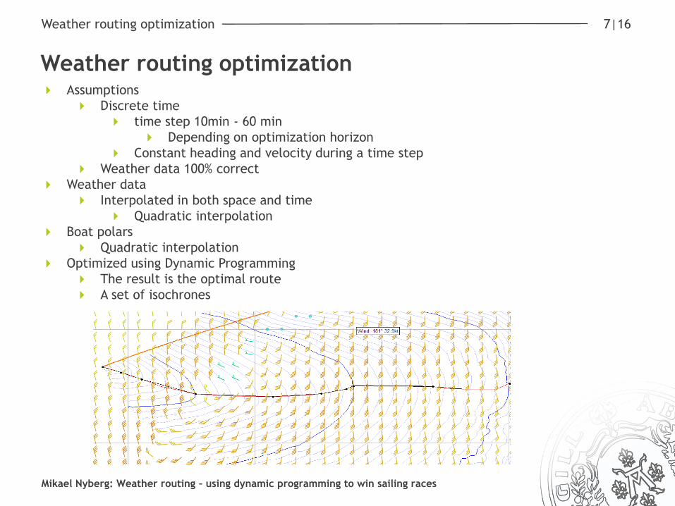
Assumptions

Discrete time

time step 10min - 60 min

Depending on optimization horizon

Constant heading and velocity during a time step

Weather data 100% correct

Weather data

Interpolated in both space and time

Quadratic interpolation

Boat polars

Quadratic interpolation

Optimized using Dynamic Programming

The result is the optimal route

A set of isochrones

Mathematical model

8|16 Weather routing: Algorithm


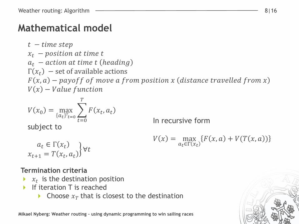
𝑉 𝑥0 = max𝑎𝑡 𝑇𝑡=0 𝐹 𝑥𝑡, 𝑎𝑡

𝑇

𝑡=0

subject to

𝑎𝑡 ∈ Γ 𝑥𝑡𝑥𝑡+1 = 𝑇 𝑥𝑡, 𝑎𝑡

∀𝑡

In recursive form

𝑉 𝑥 = max

𝑎𝑡∈Γ 𝑥𝑡𝐹 𝑥, 𝑎 + 𝑉(𝑇 𝑥, 𝑎 )

𝑡 − 𝑡𝑖𝑚𝑒 𝑠𝑡𝑒𝑝 𝑥𝑡 − 𝑝𝑜𝑠𝑖𝑡𝑖𝑜𝑛 𝑎𝑡 𝑡𝑖𝑚𝑒 𝑡 𝑎𝑡 − 𝑎𝑐𝑡𝑖𝑜𝑛 𝑎𝑡 𝑡𝑖𝑚𝑒 𝑡 ℎ𝑒𝑎𝑑𝑖𝑛𝑔

Γ 𝑥𝑡 − set of available actions 𝐹 𝑥, 𝑎 − 𝑝𝑎𝑦𝑜𝑓𝑓 𝑜𝑓 𝑚𝑜𝑣𝑒 𝑎 𝑓𝑟𝑜𝑚 𝑝𝑜𝑠𝑖𝑡𝑖𝑜𝑛 𝑥 𝑑𝑖𝑠𝑡𝑎𝑛𝑐𝑒 𝑡𝑟𝑎𝑣𝑒𝑙𝑙𝑒𝑑 𝑓𝑟𝑜𝑚 𝑥

𝑉 𝑥 − 𝑉𝑎𝑙𝑢𝑒 𝑓𝑢𝑛𝑐𝑡𝑖𝑜𝑛

Termination criteria

𝑥𝑡 is the destination position

If iteration T is reached

Choose 𝑥𝑇 that is closest to the destination

9

Complexity

The number of points (states) to evaluate is huge

68 discrete polar points

Can be reduced to 54 because sailing with TWA <36° or >155 ° is never optimal due to VMG (Velocity Made Good)

Reasonable assumptions about directions can be made

Never optimal to sail >75° off the direct course towards the finish

Reduces the number of points/time step down to 30 per time step

Using 10 minute discretization, a 6 hour route still consists of 1.5*1053 point evaluations

To reduce the search space the space is divided into sectors and only the point furthest away from the start, in each sector, is used in the next iteration

By pruning the states and only leaving the ones furthest from the starting point reduces the number of points for a 24 hour route to around 5 000 000

This pruning creates isochrones for each time step

This reduces complexity from O(N2) to O(N)

The choice of number of sectors defines N

Sector size is variable with distance to starting point to reduce sector width far away from the start


9|16 Weather routing: Complexity

10

Reducing complexity


10|16 Weather routing: Complexity

Optimal route

Best in sector

Terminated node

Sector boundary

Isochrones

Shortest distance

to destination

11

“Optimal” routing

The underlying mathematical model is a deterministic dynamic programming formulation

To reduce computational complexity in order to reduce run time the following (heuristic) assumptions have been made:

Reducing the number of points using the sector method described

Assuming reasonable headings in relation to the destination

Valid if no obstacles are present between starting point and destination

Calculate optimal upwind/downwind VMG and only use TWAs in close proximity of optimal TWA when destination bearing is <36° or >155°

The assumptions make this approach heuristic because optimality can’t be guaranteed


11|16 Weather routing: “Optimal” routing

12

Limitations

The optimization assumes 100% correct weather forecasts

Stochastic weather routing models exist but are seldom used

because stochastic weather forecasts are hard to come by

Uncertainties in forecasts can be included by running multiple

optimizations with different parameter settings

The assumptions made to reduce search space may cause weird

behavior if land masses are situated along the route

The optimization does not consider the ”riskiness” of a route

Human knowledge is needed for the risk assessment

Optimization horizon length can greatly affect optimal routes

If the destination is beyond the optimization horizon human

knowledge is needed to analyze the results


12|16 Weather routing: Limitations

13

Illustrative examples – riskiness and horizon length


13|16 Weather routing: Illustrative examples

Route: Ambrose Lighthouse – Lizard Point

2 days

5 days

8 days

14

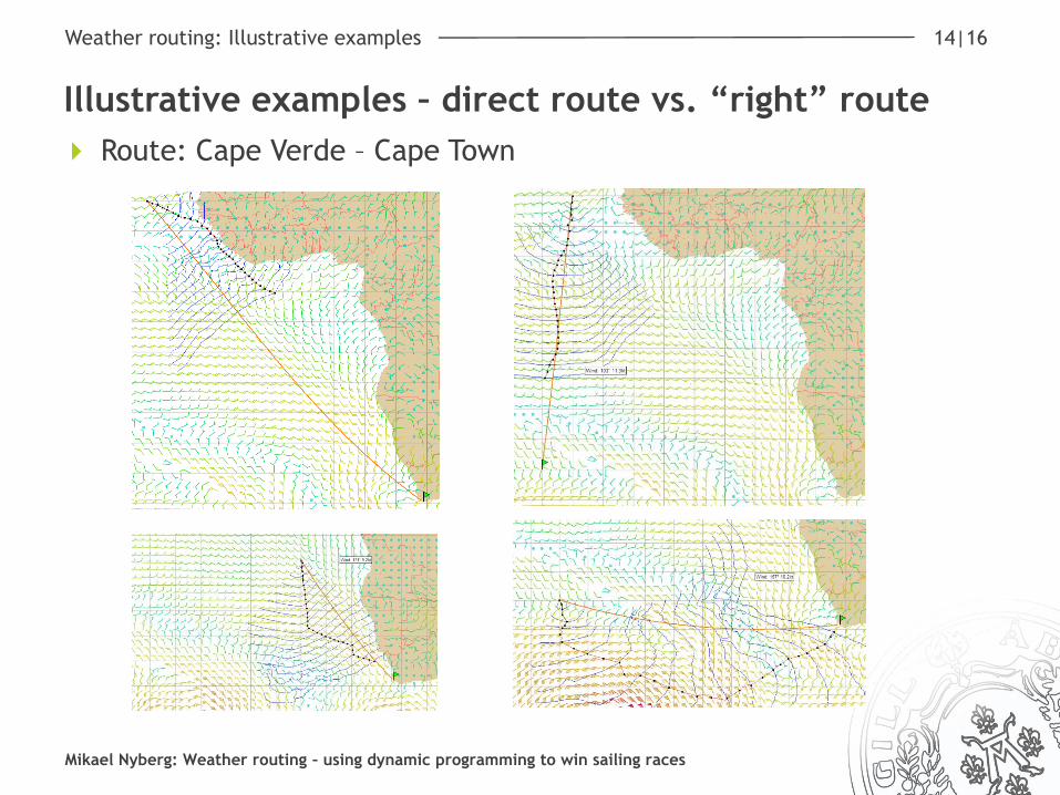
Illustrative examples – direct route vs. “right” route


14|16 Weather routing: Illustrative examples

Route: Cape Verde – Cape Town

15

Conclusions

The deterministic dynamic programming model is both efficient

and accurate

For virtual sailing the model produces extremely good routing

9 out of 10 leg winners in last Virtual Volvo Ocean Race

used this routing software

Players also used expensive ”real” weather routing

software for the virtual race

It is easy to tailor the software for real sailing by including:

Wave and current models

Multirun capability with adjustable parameters

Improved sail management

Polar import/tuning

NMEA interface to get communicate with onboard instruments


15|16 Conclusions

16

Thank you!

Questions?


16|16 Questions

Weather routing using dynamic programming to win...

Documents

Transcript of Weather routing using dynamic programming to win...