Wear Profile of the Kidd Mine Pastefill Distribution...
124
Wear Profile of the Kidd Mine Pastefill Distribution System Maureen Aileen McGuinness Department of Mining and Materials Engineering McGill University, Montreal October 2013 A thesis submitted to McGill University in partial fulfillment of the requirements of the degree of Master of Engineering © Maureen Aileen McGuinness 2013
Transcript of Wear Profile of the Kidd Mine Pastefill Distribution...

Wear Profile of the Kidd Mine Pastefill Distribution System
Maureen Aileen McGuinness
Department of Mining and Materials Engineering
McGill University, Montreal
October 2013
A thesis submitted to McGill University in partial fulfillment of the requirements of the degree of
Master of Engineering
© Maureen Aileen McGuinness 2013

Wear Profile of the Kidd Mine Pastefill Distribution System: Master's Thesis Page i Maureen McGuinness October 2013
DEDICATION
In memory of my father and his red pen and
For my mother who nurtured my belief in myself
Wear Profile of the Kidd Mine Pastefill Distribution System: Master's Thesis Page ii Maureen McGuinness October 2013
ABSTRACT / ABSTRAIT
Pipeline wear in the Kidd Mine pastefill distribution system has become one of the main challenges of
this state of the art, 400 t/h paste backfill plant commissioned, in 2004, at the Xstrata Kidd Mine, in
Timmins Ontario. The pastefill produced is a mixture of sand, tailing and binder which is non-settling
when transported in the pipeline due to its high percent solids concentration and fines content. The
transportation of this material underground, by 250NB (8 inch) diameter pipeline, resulted in high pipe
wear rates which increased maintenance costs, operational downtime and affected the flow profile of the
paste in the system.
Wear theory shows that the pipe wear rate is not a parameter of a particular slurry or pipe material, but is
a result of the overall wear system which includes the pipe, the material transported and the flow regime.
A review of the factors affecting wear indicates that velocity is considered to be the dominant factor, with
other key factors including slurry concentration, corrosion and particle shape and size. Since most slurry
transport is done at low solids concentration, there is little literature about pipe wear involving high
density slurries, such as pastefill.
The wear profile of the Kidd Mine pastefill system was developed by examining the wear system as a
whole, focusing on the key wear factors. In-situ wear data was analysed to understand the wear pattern
throughout the piping system and over time. Flow analysis was performed through hydraulic modeling. A
PSI Pill was used to determine the friction losses throughout the system and to incorporate these in the
system flow model. Material characterization and laboratory investigation using a rotary wear tester
support the characterisation of the wear found in the in-situ test work.
L’usure de la tuyauterie dans le système de distribution de remblai en pâte pour la mine Kidd est devenue
un des principaux défis pour l’usine avant-garde de remblayage de 400 t/h, construit en 2004 par Xstrata -
Kidd Mine à Timmins en Ontario. Le remblai en pâte produit est un mélange de sable, de résidus miniers
et de liant; sans sédimentation lors du transport dans la tuyauterie en raison de sa forte concentration en
matières solides et sa teneur en fines. Le transport souterrain de ce matériel par tuyauterie de 8 pouces a
donné lieu à un taux d'usure élevé des tuyaux ce qui a augmenté les coûts de maintenance, créé des
interruptions opérationnelles et influencé le régime d'écoulement de la pâte dans le système.
Wear Profile of the Kidd Mine Pastefill Distribution System: Master's Thesis Page iii Maureen McGuinness October 2013
La théorie sur l’usure montre que le taux d'usure du tuyau n'est pas dû à un paramètre particulier du
remblai ou de la tuyauterie, mais est le résultat de l'ensemble du système qui inclut le tuyau, le matériel
transporté et le régime d'écoulement. Un examen des facteurs d’influence indique que le facteur dominant
soit la vitesse d’écoulement. D’autres facteurs clés incluent la concentration de la pâte, la forme et la taille
des particules, ainsi que le niveau de corrosion. Parce que la plupart des systèmes de transport de pulpe
sont faite à une faible concentration de solides, il y a très peu de littérature sur l’usure des systèmes à
haute densité, comme le remblai en pâte.
Le profil d'usure du système de remblai en pâte pour la mine Kidd a été développé par l'examen du
système dans son ensemble, en mettant l'accent sur les facteurs d'usure clés. Les données d'usure in situ
sont analysées pour comprendre les tendances d'usure dans le système de tuyauterie et par rapport au fil
du temps. L'analyse des débits a été réalisée grâce à la modélisation hydraulique. Une PSI Pill a été utilisé
pour déterminer les pertes de charges dans le système et de les incorporer dans le modèle d’écoulement
du système. La caractérisation des matériaux et les analyses de laboratoire à l'aide d'un système de mesure
d'usure rotatif soutiennent la caractérisation de l'usure trouvée à travers les tests in situ.

Wear Profile of the Kidd Mine Pastefill Distribution System: Master's Thesis Page iv Maureen McGuinness October 2013
ACKNOWLEDGEMENTS
The author’s husband, Eric Maag, and children, Torrin and Brennan, for agreeing to be uprooted so
that the author could go back to school and supporting her throughout the process.
Dr Hassani, thesis supervisor, for his guidance and support of this line of backfill study and for
providing financial support.
Xstrata - Kidd Mine for allowing and supporting study and publication of this thesis, providing paste
characterisation data and for the loan of the rotary wear tester for this study.
Guy Pelchat, Gess Lemire, Adrian White and the pastefill team at Kidd and Lafarge for working
endlessly to ensure the success of the Kidd Mine pastefill operation and providing much help with the
PSI Pill testing campaigns, in-situ wear measurement and discussion on the project.
Vicki Newman, Jason Mireault, Christian Boucher and Eric Lafreniere for diligent data collection and
compilation, material collection, in-situ wear measurements and laboratory wear testing.
Mehrdad Kermani for the continued improvement and management of the rotary wear testing
program, help with the thesis submission and for guiding the author through the wilderness that is
going back to school.
McGill undergraduates Julian Ramirez Ruiseco and Min Shik Ahn for developing the new test spool
for the rotary test and performing the wear testing diligently.
Dr. Robert Cooke for encouraging the author to start this project and for his continued support and
detailed technical review.
Paterson & Cooke for allowing the author time and financial support to complete this thesis and for
providing laboratory use, instruction and technical support.
The P&C Sudbury lab technicians, Shawn Chrétien, Dan Zantingh and Darren Nicholson who
performed many of the PSD and rheology tests.
Dr. Sean Sanders and his team for particle shape analysis.
Marty McGuinness for editorial review, unending support and motivation throughout.
Tannis and Urs Maag for encouragement and insight into academic excellence.

Wear Profile of the Kidd Mine Pastefill Distribution System: Master's Thesis Page v Maureen McGuinness October 2013
TABLE OF CONTENTS
DEDICATION i
ABSTRACT / ABSTRAIT ii
ACKNOWLEDGEMENTS iv
TABLE OF CONTENTS v
LIST OF TABLES vii
LIST OF FIGURES viii
1. INTRODUCTION 1
2. BACKGROUND AND THEORY 3
2.1 Backfill 3
2.2 Pastefill 3
2.3 Minefill at the Kidd Mine 4
2.4 Kidd Mine Paste Plant and Material Handling 5
2.5 Pastefill Recipe 7
2.6 Underground Distribution System 10
2.7 Wear Issues 14
3. LITERATURE REVIEW OF FACTORS CONTRIBUTING TO PIPELINE WEAR 16
3.1 Types of Wear 16
3.2 Wear Theory 18
3.3 Summary 26
4. PASTEFILL SYSTEM WEAR MEASUREMENT 28
4.1 In-situ Pipe Thickness Measurement 28
4.2 Wear Data Analysis 30
4.3 Summary 37
5. HYDRAULIC EVALUATION 39
5.1 Pipeline Configuration 39
5.2 Insitu Pressure Monitoring 39
5.3 PSI Pill Test Raw Data 42
5.4 PSI Pill Data Compilation 43
5.5 PSI Pill Data Analysis 47
5.6 Flow Modeling 49
5.7 Flow Model Calibration with PSI Pill Data 54
5.8 Flow Analysis 59
5.9 Summary 67
6. PASTE CHARACTERISATION 68
6.1 Tailings Particle Size Distribution 68
Wear Profile of the Kidd Mine Pastefill Distribution System: Master's Thesis Page vi Maureen McGuinness October 2013
6.2 Sand Fineness Modulus 70
6.3 Chemical Analysis and Mineralogy 72
6.4 The Kidd Mine Pastefill Rheology 74
6.5 Summary 78
7. LABORATORY WEAR MEASUREMENT 79
7.1 Original Rotary Testwork – The Kidd Mine 79
7.2 Wear Test Development at McGill University 81
7.3 Rotary Wear Test Results 88
7.4 Summary 89
8. WEAR PROFILE DISCUSSION 91
8.1 Summary 93
9. FUTURE WORK 94
Appendix A : Pipeline System Pressure Calculation A.1
Appendix B : PSI Pill Test Logs B.1
Appendix C : Paste Charaterisation C.1
Appendix D : Rotary Wear Test Reports D.1
Appendix E : References E.1
Wear Profile of the Kidd Mine Pastefill Distribution System: Master's Thesis Page vii Maureen McGuinness October 2013
LIST OF TABLES
Table I: Piping installed in the Kidd Mine paste system ............................................................................ 10
Table II: Comparison of the ASME 31.4 and ASME 31.3 standard minimum wall thickness calculation
for the Kidd Mine pastefill system mainline ............................................................................................... 14
Table III: Variables related to the rate of erosion - as found in (Faddick 1975) ......................................... 19
Table IV: Parameters of the Kidd Mine pastefill system that characterize the pipeline system wear ........ 28
Table V: Wear rate data set distribution ..................................................................................................... 30
Table VI: Characteristics of the Kidd Mine pastefill distribution system................................................... 40
Table VII: Pour data for the PSI Pill tests ................................................................................................... 41
Table VIII: Pressure calculation for the hydraulic model of stope 63-822-ST ........................................... 51
Table IX: Calculated height of paste interface in the surface – 1600 borehole .......................................... 62
Table X: Esker sand mineralogy ................................................................................................................. 72
Table XI: McIntyre tailings mineralogy ..................................................................................................... 73
Table XII: Sand and McIntyre tailings and Kidd Creek tailings minerals sorted by hardness and compared
to steel hardness .......................................................................................................................................... 74
Table XIII: Rotary test cycle ....................................................................................................................... 86
Table XIV: Rotary test results .................................................................................................................... 88
Table XV: Trends in the Kidd Mine paste pipeline wear compared to slurry pipeline wear ...................... 91
Table XVI: The Kidd Mine wear profile components ................................................................................ 92

Wear Profile of the Kidd Mine Pastefill Distribution System: Master's Thesis Page viii Maureen McGuinness October 2013
LIST OF FIGURES
Figure 1: Components of the pipeline wear profile ..................................................................................... 1
Figure 2: The Kidd Mine material handling and pastefill system flow diagram – taken from McGuinness
and Bruneau (2008) ....................................................................................................................................... 7
Figure 3: Pastefill discharge showing the thick consistency of the the Kidd Mine pastefill (photo by
Xstrata – Kidd Mine) .................................................................................................................................... 8
Figure 4: The Kidd Mine pastefill distribution system - taken from McGuinness & Cooke (2011) .......... 12
Figure 5: Components of a pastefill distribution system ............................................................................ 12
Figure 6: Causes of wear in slurry systems (based on Truscott 1979) ....................................................... 16
Figure 7: Illustration of Steward / Sauermann definition of erosion and corrosion. Based on (Steward
and Spearing 1992). .................................................................................................................................... 17
Figure 8: Four general modes of wear with erosion further expanded into its subgroups. Based on
Budinski (2007) .......................................................................................................................................... 18
Figure 9: Effect of flow regime on pipeline abrasion: a) full-flow b) free-fall (Wang 2011)..................... 22
Figure 10: Histogram of all wear rate results retained in the Kidd Mine wear rate data base .................... 31
Figure 11: Schematic of pooling groups by distance from up-hole ............................................................ 32
Figure 12: Average wear rate vs % distance along the loop ....................................................................... 32
Figure 13: Interval plot of average wear rate vs % distance from uphole .................................................. 33
Figure 14: Examination by level of wear rate vs distance along the horizontal loop ................................. 34
Figure 15: Wear rate by level ...................................................................................................................... 35
Figure 16: Interval plot of wear rate by level .............................................................................................. 35
Figure 17: Wear rate by year....................................................................................................................... 36
Figure 18: Interval plot of wear rates grouped by year ............................................................................... 37
Figure 19: Taken from the Camiro/PAR Innovation Website - a) the PSI Pill next to a golf ball and b)
the basket catcher at the end of the pipeline (Camiro 2004) ....................................................................... 39
Figure 20: Location of PSI Pill test stopes and examples of raw PSI Pill pressure data charts ................. 41
Figure 21: Annotated raw PSI Pill data for the 66-745-ST pour on July 7, 2007 ....................................... 42
Figure 22: Joining the peaks and valleys of the raw PSI Pill data ............................................................. 44
Figure 23: 63-822-ST stope raw pressure vs time data with peak/valley approximation overlaid ............. 45
Figure 24: 75-905-ST stope raw pressure vs time data with peak/valley approximation overlaid ............. 45
Figure 25: 66-GW1-ST stope raw pressure vs time data with peak/valley approximation overlaid ......... 46
Figure 26: 66-745-ST stope raw pressure vs time data with peak/valley approximation overlaid ............. 46
Figure 27: Two PSI Pill tests done 4 minutes apart in the 66-GW1-ST stope ........................................... 47
Figure 28: Comparison of PSI Pill reading to permanent pressure gauges in the system .......................... 48
Figure 29: Pictorial representation of the energy equation components and a breakdown of piping sections
to apply conservation of energy equation ................................................................................................... 50
Figure 30: Hydraulic head ......................................................................................................................... 52
Figure 31: Hydraulic models of the four stopes ......................................................................................... 53
Figure 32: Effect of piping length on last level on the HGL of the 75-905-ST stope ................................ 54

Wear Profile of the Kidd Mine Pastefill Distribution System: Master's Thesis Page ix Maureen McGuinness October 2013
Figure 33: 63-822-ST flow model calibrated with PSI Pill pressure data .................................................. 55
Figure 34: 70-905-ST flow model calibrated with PSI Pill pressure data ................................................. 55
Figure 35: 66-GW1-ST flow model calibrated with PSI Pill pressure data ............................................... 56
Figure 36: 66-745-ST flow model calibrated with PSI Pill pressure data ................................................. 56
Figure 37: Stope 63-822-ST comparison by segment of original model vs updated model with actual
pressure losses calculated with PSI Pill ...................................................................................................... 57
Figure 38: Stope 75-905-ST comparison by segment of original model vs updated model with actual
pressure losses calculated with PSI Pill ...................................................................................................... 58
Figure 39: Stope 66-GW1-ST comparison by segment of original model vs updated model with actual
pressure losses calculated with PSI Pill ...................................................................................................... 58
Figure 40: Stope 65-745-ST comparison by segment of original model vs updated model with actual
pressure losses calculated with PSI Pill ...................................................................................................... 59
Figure 41: Friction losses vs time as measured in terms of system throughput ......................................... 60
Figure 42: Pressure loss versus distance travelled by PSI Pill .................................................................... 61
Figure 43: Pressure loss versus distance travelled by test ........................................................................... 61
Figure 44: Comparison of average system velocities for the two models over time (throughput) ............ 63
Figure 45: Velocity range in the horizontal loops - divided by location in the system ............................. 64
Figure 46: Velocity range in the boreholes - divided by location in the system ........................................ 64
Figure 47: Temperature gain vs distance travelled .................................................................................... 65
Figure 48: Temperature gain vs distance travelled - by stope .................................................................... 66
Figure 49: Particle size distribution of 2012 sample of tailings, sand, final paste product and a calculated
particle size of final paste product (combined at 50:50 ratio) with no binder included .............................. 68
Figure 50: Interval plot of the average tailings fines content (%<20um) by year ..................................... 69
Figure 51: 2011 Tailings particle size results over time ............................................................................ 70
Figure 52: Sand FM by year ...................................................................................................................... 71
Figure 53: 2011 Sand FM results over time ................................................................................................ 72
Figure 54: Historical slump data 2005-2012 ............................................................................................... 75
Figure 55: Historical slump data for the Kidd pastefill plant by year ......................................................... 76
Figure 56: ASTM Slump measurements vs % solids for the Kidd paste;with and without binder (data
provided by Kidd Mine) .............................................................................................................................. 77
Figure 57: Vane yield stress vs % solids for the Kidd paste; with and without binder (provided by the
Kidd Mine) .................................................................................................................................................. 78
Figure 58: Rotary wear test borrowed from the Kidd Mine ........................................................................ 79
Figure 59: Original rotary test results by the Kidd Mine – mass loss vs time (Newman 2010) ................. 80
Figure 60: The Kidd Mine rotary wear test results – thickness loss per 100 kt paste throughput (Newman
2010) ........................................................................................................................................................... 80
Figure 61: Leaking end caps and the resulting balls of paste caused by loss of water ............................... 81
Figure 62: New cap assembly developed for rotary wear test .................................................................... 82
Figure 63: New spool filled with paste on the rotary machine ................................................................... 82

Wear Profile of the Kidd Mine Pastefill Distribution System: Master's Thesis Page x Maureen McGuinness October 2013
Figure 64: Circularity of the tailings samples 7 days in the rotary tester overlapped with day 0 results
(measured using FPIA) ............................................................................................................................... 84
Figure 65: Change in particle size distribution of tailings after 0,3 and 7 days in the rotary test ............... 85
Figure 66: Increase in % passing versus particle size during the rotary test ............................................... 85
Figure 67: Comparison of the individual rotary wear test results ............................................................... 89

Wear Profile of the Kidd Mine Pastefill Distribution System: Master's Thesis Page 1 Maureen McGuinness 119010215 October 2013
1. INTRODUCTION
In 2004, the Kidd Mine pastefill plant was commissioned and became the largest pastefill plant in
operation at that time, with an hourly operating rate of 400 t/h providing paste minefill to stopes at a
depth of 2300m. Two years later, this state of the art pastefill system was showing signs of high pipeline
wear which made the system difficult to operate due to changes in the pipeline flow and resulted in a
large strain on maintenance to replace worn pipes. This thesis examines the wear profile of the Kidd Mine
pastefill distribution system to understand the factors which characterise pipeline wear and effects of the
wear on the pastefill operation.
Wear profile can be defined in several ways since wear is a process involving many facets, as shown in
Figure 1. In the traditional sense, wear profiling involves examining the degree of material loss
throughout the surface of the component. In a pipeline, it involves tracking changes in pipe wall thickness
of pre-selected areas of the pipe throughout the distribution system. The wear profile can also be
characterised by the factors influential in causing wear. Since wear arises from the interaction between
the pipe wall and the material moving through the pipe, the pipeline wear profile can be characterised by
the material flow behaviour in the pipe. The properties of the paste itself can be used to evaluate the wear
profile and can be further evaluated by laboratory wear testing.
Figure 1: Components of the pipeline wear profile
Pipeline Wear
Profile
In-situ pipeline wear
measurement
Flow modeling of pipeline
system
Material Characterisation
Laboratory Testing
Wear Profile of the Kidd Mine Pastefill Distribution System: Master's Thesis Page 2 Maureen McGuinness 119010215 October 2013
The examination of the wear profile will develop as follows:
Background and Theory
A review of pastefill as a backfilling method and its characteristics
The background of the Kidd Mine pastefill process and wear experience
A review of wear theory relevant to pastefill
Pastefill System Wear Profile Characterisation
Wear measurement in the field
Hydraulic evaluation of the pastefill flow in the distribution system
An examination of the characteristics of the Kidd Mine pastefill
Laboratory wear testing
Wear Profile of the Kidd Mine Pastefill Distribution System: Master's Thesis Page 3 Maureen McGuinness 119010215 October 2013
2. BACKGROUND AND THEORY
This study focussed on the pastefill application at the Kidd Mine in Timmins, Ontario. The following
sections provide a brief overview of backfill, explanation of pastefill and the history of backfill at the
Kidd Mine. It concludes with a description of the pastefill system operated at the Kidd Mine and the wear
issues that have arisen.
2.1 Backfill
Backfilling is defined as “to refill (an excavated hole) with the material dug out of it” (Oxford
Dictionary). In mining terms, the backfill or minefill process refers to the refilling of empty stopes with
waste material, usually with the goal of increasing the stability of the remaining rock around stopes by
reducing the voids underground. Other goals of minefill can be to reduce the surface disposal of tailings
by returning the waste underground and to avoid transporting waste rock to surface for disposal. There are
three types of minefill commonly used in the mining industry. In order of their development historically
they are: rockfill, hydraulic fill and pastefill1.
2.2 Pastefill
Pastefill is the most recent development in minefill, first used in the 1980’s. This high density fill is made
with full plant tailings, deslimed tailings or a combination of sand and tailings. Pastefill relies on a
minimum quantity of fines to produce a non-settling slurry which is pipelined to underground stopes
either by gravity or with aid of a pump. The solids concentration of the paste is usually above 75%, which
makes it a non-Newtonian fluid which, at typical paste flow velocities (<5 m/s), exhibits laminar flow
properties. This helps in the transportation of the fill without excessive amounts of water. There is little,
to essentially no, bleed water from the fill. Binder is added to the fill to avoid the risk of liquefaction.
Liquefaction is a condition that is possible when a stope full of pastefill is shaken enough to transform the
paste (which had a certain amount of cohesion inherent to it) into a liquid state. In the liquid state, the full
stope height of head pressure is developed. A similar situation in hydraulic fill can occur if the transport
water is not able to drain out of the fill once it is placed in the stope.
Distribution systems for pastefill rely on constant slow flowing feed. Friction losses during transport are
higher for pastefill than hydraulic fill due to the fines content in the paste (Cooke 2007). The fines help
keep the particles in suspension. A rule of thumb in the industry is that a minimum of 15% fines (< 20μm
material) should be present in the pastefill to keep the particles from settling (Landriault and Lidkea
1 Rockfill is generally cemented waste rock, placed by truck or conveyor; hydraulic fill is generally cemented
classified tailings (fines removed), placed by pipeline
Wear Profile of the Kidd Mine Pastefill Distribution System: Master's Thesis Page 4 Maureen McGuinness 119010215 October 2013
1993). In practical terms, this means that flow in a pipeline full of paste can be reinitiated after a period of
time because the solids are still in suspension (within limitations of the hydration reactions).
Pastefill is noted to have a more complex operating system than hydraulic fill and rockfill but one that
allows for higher fill quality controls than its counterparts. One of the major benefits of pastefill is its
quicker cycle time for the fill process which has a positive impact on the overall mining cycle. Its use of a
significant portion of the fines, and even all of the fines in some cases, results in much less on surface
fines storage requirements.
2.3 Minefill at the Kidd Mine
The Kidd Mine is a copper-zinc mine which started as an open pit in 1965 and moved underground in
1973. Along with a ramp, there was shaft access to the mine for personnel transport and through which
ore was hoisted to surface. Yu (1983) describes the mining method at the Kidd Mine as sublevel blasthole
stoping with and without rib pillers depending on the mining area. Minefill was an integral part of the
mining sequence. Yu explains that the Kidd Mine ran a cemented rockfill system throughout most of its
underground mining life. Waste rock from the open pit was sized to contain 75% aggregate and 25% fines
with extra fines being removed in the plant before the fill was sent underground. The rock was
transported to the stope via orepasses, haulage and on several levels by an extensive conveyor system.
Cement slurry was added to the rock underground as it was dumped into the stope or at a mixing station
where it was combined with aggregate in batches before haulage to the stope.
Rockfill was gradually phased out when the mine converted to pastefill for the mine expansion to depth,
in 2004. Kidd Mine had reached the 6800 level (at 2000 m depth) and was developing the first part of a
planned expansion to the 10200 level (at over 3000 m depth). One significant change in the mining
philosophy was the adoption of pastefill as the minefill for the mine at depth. There were several reasons
for the switch to pastefill, as explained by Lee and Pieterse (2005):
Due to the increased pressures at depth, quick filling of the voids was deemed critical to the
success of the mining strategy. Pastefill has a shorter cycle time than rockfill or hydraulic fill
processes as stopes can be filled quickly and do not have to wait for drainage before they
consolidate.

Wear Profile of the Kidd Mine Pastefill Distribution System: Master's Thesis Page 5 Maureen McGuinness 119010215 October 2013
The high quality control and homogeneity of pastefill was also a key factor for successful filling
and subsequent mining at depth. The paste could meet the high strength requirement of the mine
for ground control and sill exposure.
Economic analysis showed that the costs of rockfilling at depth were higher than those for
pastefill.
Once in operation, the pastefill system was expanded to service the existing, upper mine levels due to the
savings in fill cycle time and the benefits of a high quality fill for stabilisation and tightfilling of old
stopes. Uncemented, ungraded, waste fill is still used throughout the mine to fill stopes that will not be
exposed in the future.
2.4 Kidd Mine Paste Plant and Material Handling
The configuration of the Kidd Mine paste plant was influenced by the fact that the mine site was 50 km
away by road from the concentrator – the traditional source of tailings for pastefill. After much debate, it
was decided that, instead of pumping or transporting the tailings slurry from the Kidd concentrator to the
mine site, tailings, in a solid format, were to be excavated from a closed out tailings pond and trucked to
the mine site for processing (Landriault, Brown et al. 2000, Lee and Pieterse 2005). The tailings source
initially was from the Pamour T3 tailings dam. The excavation moved to the McIntyre tailings pond in
2006 to take advantage of the shorter haulage distance. To offset some of the costs of excavating the
tailings and to refine the particle size distribution of the final paste product, a portion of the tailings was
substituted with sand, an easier product to excavate and transport (Lee and Pieterse 2005). This
fundamental decision on source material determined the type of paste plant to be built at the Kidd Mine
site - a batch plant. Each excavation site is a process on its own and includes excavation, screening and
stockpiling. These processes are pictured in Figure 2, showing both the off-site and on-site processes.
Material preparation is done in the summer months with haulage from the storage piles continuing year
round (McGuinness and Bruneau 2008). Material is trucked to the pastefill plant around the clock,
throughout the year.
The paste plant at the Kidd Mine is fed by two parallel feed systems to handle the tailings and sand as it
arrives on site by truck. The products are stored separately in two 20,000 tonne capacity heated domes.
During production, loaders haul material from the domes to dedicated conveyors which feed the paste
plant.

Wear Profile of the Kidd Mine Pastefill Distribution System: Master's Thesis Page 6 Maureen McGuinness 119010215 October 2013
Wear Profile of the Kidd Mine Pastefill Distribution System: Master's Thesis Page 7 Maureen McGuinness 119010215 October 2013
Previous Page:
Figure 2: The Kidd Mine material handling and pastefill system flow diagram – taken from McGuinness
and Bruneau (2008)
The tailings cannot be stored in a silo due to its relatively high moisture content (14%). Instead, the
tailings is directed by conveyor to a continuous mixer which adds enough water to bring it into a slurry
state at around 22 to 24% moisture content. This slurry fills an agitated tank which feeds the tailings
weigh scale. Sand is stored, as is, in two sand silos which feed the sand weigh scale. The binder is stored
in two 200 tonne silos. Screw conveyors transport the binder to a third weigh scale. There is a fourth
weigh scale for water addition.
When operating, the weigh scales are filled and dump into the batch mixer when it is ready to accept
material. The batch mixer is an Arcen twin-shaft mixer with bottom discharge gate. The paste is mixed
for approximately 2 minutes and the consistency of the paste is adjusted to achieve a pre-determined
power draw, with water added as necessary. The final paste product is shown in Figure 3. The prepared
batch is dumped into a gob hopper which funnels the paste into the pastefill distribution system. Initially,
there were two gob hoppers, as shown in Figure 2, but wear of the surface boreholes has resulted in two
new boreholes being drilled and fed solely from the #1 gob hopper.
The batching system produces 400 t/h paste, with a maximum daily production of 9600 tonnes. The
pastefill operation regularly produces over 8000 t/d and averages a 1.3 Mt yearly production rate.
2.5 Pastefill Recipe
As mentioned in Section 2.4, the Kidd Mine pastefill recipe includes tailings, sand, binder and water. The
tailings source has changed since commissioning the plant. Both sources were gold mine tailings. The
change of location was beneficial as it reduced the distance of the tailings haulage considerably. The sand
source has remained the same for the duration of the paste production. It is an esker sand pit located
around 15 km from the mine site. The binder is a premixed blend of 90% slag and 10% Portland cement,
from Lafarge. It is trucked in from the Lafarge plant in Spragg, Ontario.
The pastefill recipe respects the conditions needed for good strength development (short term and long
term, as required) and for effective transportation. The criteria that must be met include:

Wear Profile of the Kidd Mine Pastefill Distribution System: Master's Thesis Page 8 Maureen McGuinness 119010215 October 2013
Paste fines content (for transport): minimum 15% passing 20μm
Binder content (for pastefill strength): 2-4.5%
Paste solids content (for transport and strength): 80%-83%.
Figure 3: Pastefill discharge showing the thick consistency of the the Kidd Mine pastefill (photo by Xstrata – Kidd Mine)
2.5.1 Fines Content
The fines content is controlled by the tailings to sand ratio used in the batch. The industry standard
recommends a minimum fines content of 15% passing 20μm. As a control measure to ensure the
minimum content is achieved, even with normal process variation in fines content, the Kidd specification
for fines in the pastefill was increased to 20% passing 20μm.
The tailings provide the fines to the mix. The excavated tailings are blended so that they contain between
40 and 60% fines (-20μm material). The sand provides coarser particles which help create a well graded
final paste product (Lee and Pieterse 2005). This is important to optimize paste strength, flowability and
particles suspension.
Since 2010, the tailings fines range has been increased to 45-55% passing 20μm in order to increase the
volume of tailings that can be recovered from the tailings site and the pastefill recipe has been adjusted as
necessary to meet strength and flow requirements.

Wear Profile of the Kidd Mine Pastefill Distribution System: Master's Thesis Page 9 Maureen McGuinness 119010215 October 2013
2.5.2 Binder Content
The Kidd Mine has defined the following strength criteria for the pastefill. The required strengths vary
by final usage of the fill and can range between 2% and 4.5% binder content (White 2013). The binder is
a slag-portland cement blend which provides good long term strength with acceptable short term strength
gain which meets the mining cycle requirements. The binder also adds fines to the pastefill and does have
lubrication properties. This is seen during operation, where pours containing high percentage binder
recipes flow easier than the low percentage binder pours allowing for a higher throughput in the line.
The binder content is added on a dry basis according to the following formula:
The inclusion of sand in the pastefill has resulted in lower binder requirements to meet the specified
pastefill strengths.
2.5.3 Solids Content
The optimum solids content of the paste requires a balance between the water needed to transport the
solids through the pipeline and the effect of water content on the pastefill strength. Solids content is the
parameter that is most modified on an operational basis in response to changes in the system. The paste
yield stress is modified by increasing or decreasing the solids content of the pastefill, which changes the
flow in the pipeline. The relationship between percentage solids content and the yield stress is non-linear
(Henderson, Revell et al. 2005) so that small changes in water addition have a large influence on the
flowability of the paste.
The solids content is calculated according to the following formula:
%������ = ��
�� + �� + ��
where,
mb=mass of binder
mt=mass of tailings
ms=mass of sand
Equation 2-1
%������ =
�� + �� + ��
�� + �� + �� + ��
where,
mw=mass of water
Equation 2-2

Wear Profile of the Kidd Mine Pastefill Distribution System: Master's Thesis Page 10 Maureen McGuinness 119010215 October 2013
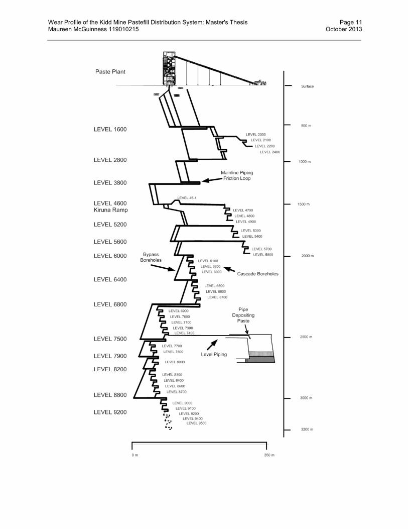
2.6 Underground Distribution System
The Kidd pastefill plant does not contain a paste pump. The transportation of the pastefill through the
pipeline is governed solely by gravity. This is possible because of the high vertical to horizontal ratio of
the distribution system, as shown in Figure 4. While the horizontal expanse of the levels is only in the
range of 300 m, the vertical depth is over 3000 m at the bottom creating a 10:1 vertical to horizontal ratio.
There is over 5 km of piping in the pastefill system. At the lower levels, it can take 1 to 2 hours for the
paste to reach the stope.
The pipeline system is broken down into three main parts. The types of pipes used for each part change
according to their function, as shown in Table I. The pipe schedule used in the different parts of the
system is chosen based on their pressure rating. The pressure is greatest at the bottom of the long
boreholes and gradually decreases to atmospheric pressure as the paste leaves the pipeline to freefall into
the stope. An example of a pastefill distribution system on a level is shown in Figure 5 with key elements
identified.
Table I: Piping installed in the Kidd Mine paste system
Piping
Type
Purpose Pipe Type Pipe Diameter Pipe Schedule Pressure
Rating
Boreholes Connect levels;
Higher wear resistance
Microtech
W65
9 inch OD 19.0 mm wall
(0.750 inch wall)
10 MPa
(1500 psi)
Mainline
Piping
Horizontal loops
connecting boreholes;
Higher pressure areas;
Friction loops (to
reduce paste velocity);
API 5L X52 200NB
(219 mm OD)
Standard 8 inch
(8.625 in OD)
Schedule 80
12.7 mm wall
(0.500 inch wall)
10 MPa
(1500 psi)
Level
Piping
Horizontal pipe runs
connecting mainline to
the stopes
Lower pressure areas
API 5L X52 200NB
(219 mm OD)
Standard 8 inch
(8.625 in OD)
Schedule 40
8.2 mm wall
(0.322 inch wall)
6.5 MPa
(950 psi)
Wear Profile of the Kidd Mine Pastefill Distribution System: Master's Thesis Page 11 Maureen McGuinness 119010215 October 2013

Wear Profile of the Kidd Mine Pastefill Distribution System: Master's Thesis Page 12 Maureen McGuinness 119010215 October 2013
Previous Page:
Figure 4: The Kidd Mine pastefill distribution system - taken from McGuinness & Cooke (2011)
Changes to the original piping system were made in response to high pipeline wear rates. Smaller
diameter pipe was used selectively in the loops and on the level piping to increase friction in the system.
Since 2010, new boreholes have been drilled and lined with API 5L X52 schedule 40 pipes lined with
ceramic.
The maintenance program for the underground distribution system includes visual inspection, pipe wall
thickness measurement, borehole inspection and tonnage tracking. The tonnage passed through each pipe
part is tracked based on the paste production and pipe route for each paste pour. Sections are flagged for
inspection based on an established pipeline wear rate and confirmed through non-destructive testing
(NDT). Pipe wall thickness measurement program, using an ultrasonic gauge, is performed quarterly and
the results are tracked in the maintenance database. Visual inspection of all level and loop piping during
pouring ensures that any leaks or other problems are dealt with promptly.
Figure 5: Components of a pastefill distribution system
2.6.1 Minimum Pipe Wall Thickness Requirement
The thickness at which the pipes required changing is based on the minimum internal pressure design
wall thickness required to meet the pressure rating of the system. This pressure rating takes into account
Wear Profile of the Kidd Mine Pastefill Distribution System: Master's Thesis Page 13 Maureen McGuinness 119010215 October 2013
the pipe material and its allowable stresses, the type of connection, pipe size, wear and corrosion and
applicable safety factors. There are different standards which are used to determine the internal pressure
design wall thickness. The two used for steel piping are ASME B31.3 Process Piping Standard and
ASME B31.4 Pipeline Transportation Systems for Liquids and Slurries (formerly known as ASME
B31.11).
The Kidd pastefill mainline piping system is rated for 10MPa (1450 psi) and follows the ASME B31.4
standard for pipelines (Xstrata internal communication). However, there are many in the backfill industry
who recommend using the more stringent ASME B31.3 Process Piping Standard for backfill piping as the
pipeline is installed throughout the workings of the mine and is more akin to in-plant process piping and
their requirements for maintenance and safety than to the overland pipelines targeted in the ASME B31.4
Standard (Cooke and Paterson 2013).
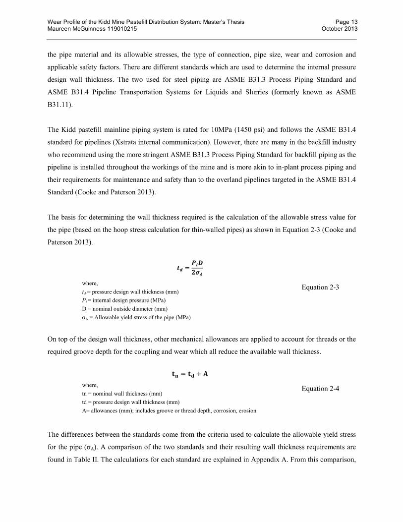
The basis for determining the wall thickness required is the calculation of the allowable stress value for
the pipe (based on the hoop stress calculation for thin-walled pipes) as shown in Equation 2-3 (Cooke and
Paterson 2013).
On top of the design wall thickness, other mechanical allowances are applied to account for threads or the
required groove depth for the coupling and wear which all reduce the available wall thickness.
The differences between the standards come from the criteria used to calculate the allowable yield stress
for the pipe (σA). A comparison of the two standards and their resulting wall thickness requirements are
found in Table II. The calculations for each standard are explained in Appendix A. From this comparison,
�� =���
���
where,
td = pressure design wall thickness (mm)
Pi = internal design pressure (MPa)
D = nominal outside diameter (mm)
σA = Allowable yield stress of the pipe (MPa)
Equation 2-3
�� = �� + �
where,
tn = nominal wall thickness (mm)
td = pressure design wall thickness (mm)
A= allowances (mm); includes groove or thread depth, corrosion, erosion
Equation 2-4
Wear Profile of the Kidd Mine Pastefill Distribution System: Master's Thesis Page 14 Maureen McGuinness 119010215 October 2013
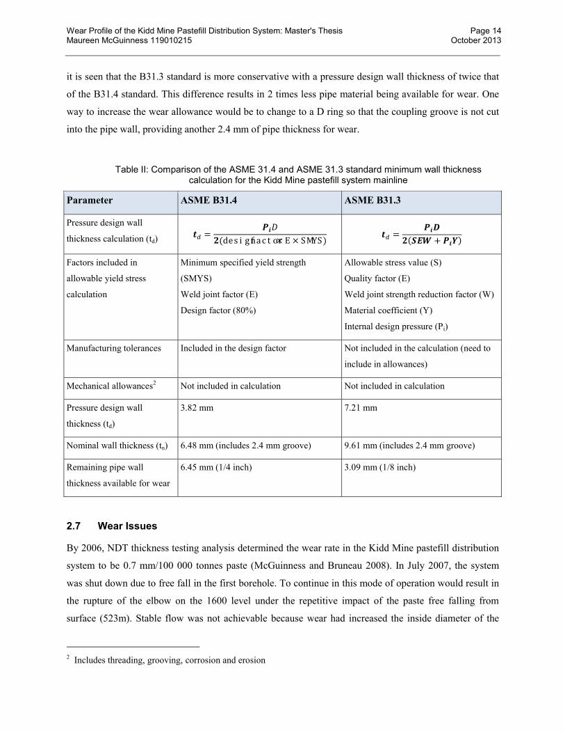
it is seen that the B31.3 standard is more conservative with a pressure design wall thickness of twice that
of the B31.4 standard. This difference results in 2 times less pipe material being available for wear. One
way to increase the wear allowance would be to change to a D ring so that the coupling groove is not cut
into the pipe wall, providing another 2.4 mm of pipe thickness for wear.
Table II: Comparison of the ASME 31.4 and ASME 31.3 standard minimum wall thickness calculation for the Kidd Mine pastefill system mainline
Parameter ASME B31.4 ASME B31.3
Pressure design wall
thickness calculation (td) �� =
���
�(designfactor× E × SMYS) �� =
���
�(��� + ���)
Factors included in
allowable yield stress
calculation
Minimum specified yield strength
(SMYS)
Weld joint factor (E)
Design factor (80%)
Allowable stress value (S)
Quality factor (E)
Weld joint strength reduction factor (W)
Material coefficient (Y)
Internal design pressure (Pi)
Manufacturing tolerances Included in the design factor Not included in the calculation (need to
include in allowances)
Mechanical allowances2 Not included in calculation Not included in calculation
Pressure design wall
thickness (td)
3.82 mm 7.21 mm
Nominal wall thickness (tn) 6.48 mm (includes 2.4 mm groove) 9.61 mm (includes 2.4 mm groove)
Remaining pipe wall
thickness available for wear
6.45 mm (1/4 inch) 3.09 mm (1/8 inch)
2.7 Wear Issues
By 2006, NDT thickness testing analysis determined the wear rate in the Kidd Mine pastefill distribution
system to be 0.7 mm/100 000 tonnes paste (McGuinness and Bruneau 2008). In July 2007, the system
was shut down due to free fall in the first borehole. To continue in this mode of operation would result in
the rupture of the elbow on the 1600 level under the repetitive impact of the paste free falling from
surface (523m). Stable flow was not achievable because wear had increased the inside diameter of the
2 Includes threading, grooving, corrosion and erosion

Wear Profile of the Kidd Mine Pastefill Distribution System: Master's Thesis Page 15 Maureen McGuinness 119010215 October 2013
pipe to the point that remaining friction in the line could no longer back the paste up into the borehole. As
proof, when the operation switched to the spare borehole, stable flow was achieved with ease.
As tonnage through the boreholes increased over time, the free fall situation described above repeated in
the boreholes further down the system. To protect the boreholes, extra lengths of pipe were installed on
the horizontal loops to provide more friction to the system which backs up the paste into the boreholes. In
some cases, smaller diameter pipes 150NB (6 inch) were installed to provide an even larger restriction,
and therefore friction, in the loops. This method is effective but increased the risk of plugging and
localised wear at the 200NB (8 inch) to 150NB reduction point.
To maintain the pipeline pressure rating, maintenance became a priority to ensure the pipes did not
exceed the wear allowance. Loop change out was performed regularly (once a year for high throughput
areas) resulting in high material and labour costs for the rework. This pattern of wear and pipe loop
replacement would continue for the life of the mine unless a more permanent solution was found.
However, there was no way to easily replace the borehole casings which represented 2/3 of the pipe
length in the system and therefore governed a majority of the friction in the system.
By 2009, the surface borehole to 1600 level had casing that was worn to the rock in places and blockages
were common as more pipe wall peeled away and obstructed the pipe. Production became unreliable. The
minefill process fell behind schedule and became a risk to the mine production.
A decision was made to find a more wear resistant pipe material to counter the wear as there was no
desire to change the type of material being used to make the paste or the production rate at which the
paste was produced. It was decided to return the system to its original state which was balanced and
provided full, steady flow throughout and to select a material that would maintain this state by being
highly wear resistant. Ceramic lined steel pipe was selected. This pipe, from Imatech, had been
successfully used in other high wear minefill systems, notably Kidd’s sister mine, Mount Isa, in Australia.
An attempt was made to remove the worn casing from the surface borehole and reline it with the ceramic
lined casing. After much effort and little success, this strategy was abandoned. Two new boreholes were
drilled and cased with the ceramic lined pipe. Plans were made to install new boreholes cased with
ceramic lined pipe in all the upper section boreholes of the mine through which almost all the paste
travels. This work is now underway.

Wear Profile of the Kidd Mine Pastefill Distribution System: Master's Thesis Page 16 Maureen McGuinness 119010215 October 2013
3. LITERATURE REVIEW OF FACTORS CONTRIBUTING TO PIPELINE WEAR
Wear is a widespread phenomenon in operations which causes important downtime and financial loss to
many industries. In pipeline operation, wear is the most important factor to the longevity of the pipeline
system. Consequently, much research has been done into the factors causing wear and the methods for
measurement and prediction of the wear with the goal to understand and minimise its impact on the
pipelining operation. However, most of the pipelining done in the world is of low density slurries. The
high density paste application has been little studied, in term of wear. A review was made of literature
pertaining to erosion, particularly in pipelines and the factors influencing pipeline wear.
3.1 Types of Wear
Several classifications of wear modes have been published over the years. With respect to slurry system
wear, there is generally a consensus as to the main types of wear that should be included in this group but
the nomenclature and grouping has varied over the years.
3.1.1 Slurry Wear Classification
In a 1979 short course on pipeline wear, Truscott (1979) divided wear in slurry systems into two main
causes: erosion and corrosion. As summarized in Figure 6, the abrasion due to solid particles is a subset
of erosion. The other cause of erosion is due to cavitation. Corrosion can be purely chemical or can have
an electro-chemical component. The use of the word abrasion in this classification relates to the removal
of pipe material due to the physical contact of the slurry solids with the pipe wall from the pipe.
Figure 6: Causes of wear in slurry systems (based on Truscott 1979)
Wear in Slurry Systems
Erosion
Solid particles -abrasive wear
Cavitaton
Corrosion
Chemical Electro-Chemical

Wear Profile of the Kidd Mine Pastefill Distribution System: Master's Thesis Page 17 Maureen McGuinness 119010215 October 2013
Faddick (1975)published a similar classification which breaks slurry pipeline wear into two main modes:
corrosion and mechanical abrasion (erosion). Both Faddick and Truscott use erosion and abrasion
interchangeably in their classification.
Steward and Spearing (1992) described a different interpretation of the definition of erosive and abrasive
wear. In this definition of slurry wear, both erosion and abrasion refer to a slurry system but differentiate
how the particles interact with the pipe wall, as shown in Figure 7. They explain, based on Sauermann’s
work, that erosion is the process by which particles impact the pipe walls (at different impact angles from
0 to 90 degrees) and the repeated impact forces small pieces of the pipe wall out of their matrix. Abrasion,
in his definition, is caused by particles sliding along the axis of the pipe wall causing small particles of
the wall to be removed (Steward and Spearing 1992).
Figure 7: Illustration of Steward / Sauermann definition of erosion and corrosion. Based on (Steward and Spearing 1992).
While Truscott alludes to abrasive wear as one mode of erosion, his model does not take into account the
impact type of wear specifically. On the other hand, the Steward / Sauermann interpretation can lead to
confusion with the solid-solid wear mode most commonly called abrasion.
Since then, the ASTM Committee G02 Wear and Erosion classification has been made that combines the
wear described by the previous authors into a comprehensive wear classification.
3.1.2 ASTM Committee G02 Wear and Erosion Classification
The ASTM Committee G02 Wear and Erosion classification divides wear modes into four large groups:
abrasive, erosion, adhesive and surface fatigue (Budinski 2007). In this classification, erosion pertains to
wear involving mixtures of fluids and solids. Most of the time, the fluid is water, as in the case of paste.
Erosion is separated from the “dry” wear situation of “abrasion” – those that do not have a fluid
component. The idea of separating sliding and impact modes is found in the model under the terms slurry
wear and impingement wear, respectively. The effect of corrosion, as another erosive wear mode, is also
erosion abrasion

Wear Profile of the Kidd Mine Pastefill Distribution System: Master's Thesis Page 18 Maureen McGuinness 119010215 October 2013
recognized in this model. Figure 8 provides a summary of this classification, detailing the sub-groups of
erosion.
Figure 8: Four general modes of wear with erosion further expanded into its subgroups. Based on Budinski (2007)
The variety of wear groups in this classification highlights the importance of first identifying the type of
wear in the pipeline in order to understand and mitigate its effect, and to choose an appropriate wear test
(Budinski 2007). While the method of transport may be the same, the mode of wear can vary greatly. For
example, Faddick explains that, while both coal and phosphate slurries are pipelined in similar manners,
the mechanism by which these lines wear vary greatly. Coal wears by corrosion while phosphate wears by
erosion (Faddick 1975).
3.2 Wear Theory
The theory of wear aims at finding a rate of material degradation for a system investigated. The wear rate
is a function of various factors. Thus, a review of the literature reveals that the determination of the
factors influencing wear and the development of the wear theory are often treated together; the resulting
theory derived from the influence of the factors was investigated.
Wear Modes
Abrasive
(Solid –solid contact)
Erosion
(Solid--liquid contact )
SlurrySolid particle
(fluid is air)
Erosion/corrosion (of protective
film)Cavitation
Impingement
Adhesive Surface Fatigue
Wear Profile of the Kidd Mine Pastefill Distribution System: Master's Thesis Page 19 Maureen McGuinness 119010215 October 2013
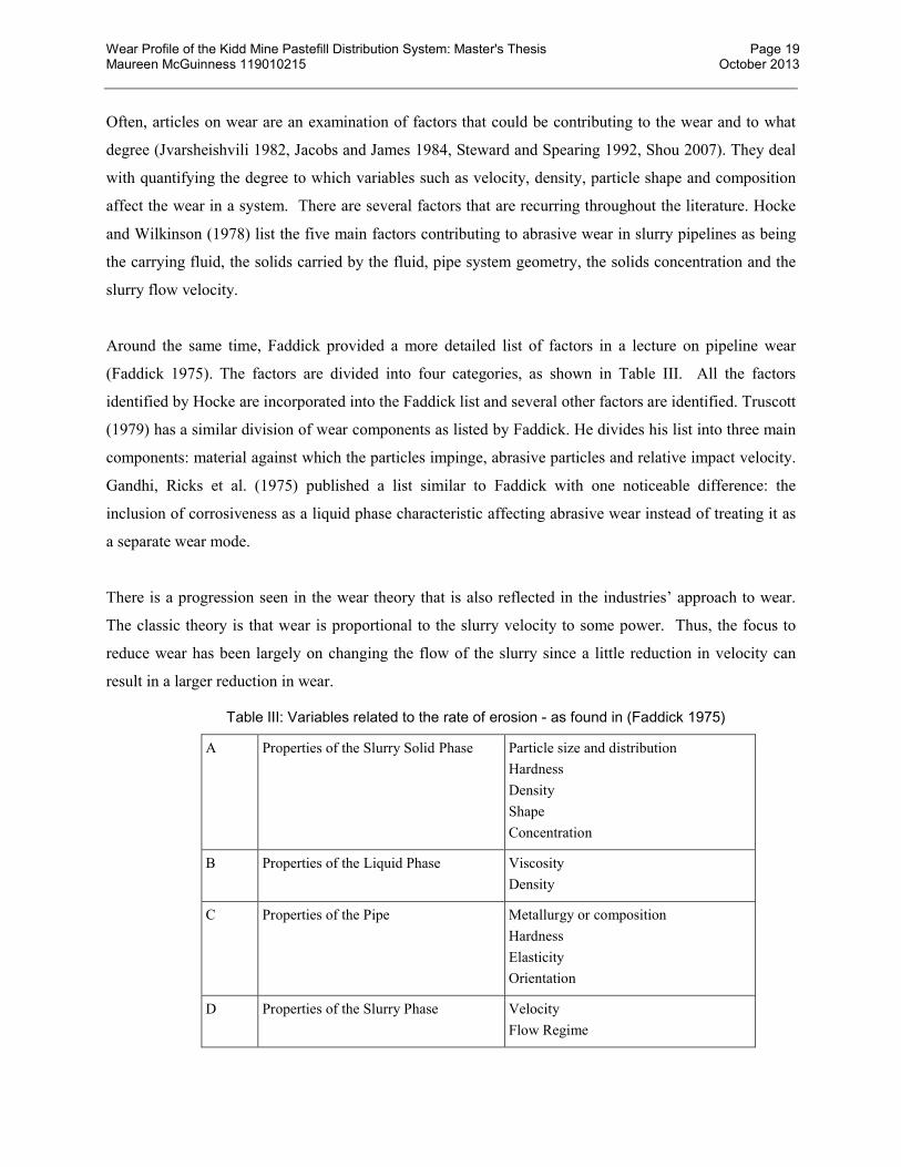
Often, articles on wear are an examination of factors that could be contributing to the wear and to what
degree (Jvarsheishvili 1982, Jacobs and James 1984, Steward and Spearing 1992, Shou 2007). They deal
with quantifying the degree to which variables such as velocity, density, particle shape and composition
affect the wear in a system. There are several factors that are recurring throughout the literature. Hocke
and Wilkinson (1978) list the five main factors contributing to abrasive wear in slurry pipelines as being
the carrying fluid, the solids carried by the fluid, pipe system geometry, the solids concentration and the
slurry flow velocity.
Around the same time, Faddick provided a more detailed list of factors in a lecture on pipeline wear
(Faddick 1975). The factors are divided into four categories, as shown in Table III. All the factors
identified by Hocke are incorporated into the Faddick list and several other factors are identified. Truscott
(1979) has a similar division of wear components as listed by Faddick. He divides his list into three main
components: material against which the particles impinge, abrasive particles and relative impact velocity.
Gandhi, Ricks et al. (1975) published a list similar to Faddick with one noticeable difference: the
inclusion of corrosiveness as a liquid phase characteristic affecting abrasive wear instead of treating it as
a separate wear mode.
There is a progression seen in the wear theory that is also reflected in the industries’ approach to wear.
The classic theory is that wear is proportional to the slurry velocity to some power. Thus, the focus to
reduce wear has been largely on changing the flow of the slurry since a little reduction in velocity can
result in a larger reduction in wear.
Table III: Variables related to the rate of erosion - as found in (Faddick 1975)
A Properties of the Slurry Solid Phase Particle size and distribution
Hardness
Density
Shape
Concentration
B Properties of the Liquid Phase Viscosity
Density
C Properties of the Pipe Metallurgy or composition
Hardness
Elasticity
Orientation
D Properties of the Slurry Phase Velocity
Flow Regime
Wear Profile of the Kidd Mine Pastefill Distribution System: Master's Thesis Page 20 Maureen McGuinness 119010215 October 2013
What is apparent from the above review of wear factors is that, while velocity remains a predominant
wear factor, many authors do acknowledge the impact of other components of wear. The solution to
reducing wear may not be as simple as velocity reduction. In fact, the classic wear-velocity relationship
did include the effect of other factors through its varying exponential component and its constant
multipliers; both of which are case specific. Steward and Spearing make this connection between the
constants in the wear-velocity relationship and other influential wear factors (Steward and Spearing 1992)
and other researchers show that the exponent is variable, even if they don’t associate it to a particular
factor.
The main wear factors that are repeated by the various authors are velocity, solids concentration, particle
shape, particle size, flow regime, corrosion and pipe material. The impact of these factors on wear will be
examined in the following sections.
3.2.1 Velocity
Velocity is considered one of the most significant factors by most authors. The accepted relationship is
that an increase in velocity results in an increase in the wear rate. Many of the experiments described by
authors have validated this trend for slurries (Steward and Spearing 1992, Gupta 1995, Patil, Deore et al.
2011). Hocke and Wilkinson expected and saw this relationship in their work on a rolling cylinder lab
wear test in 1978 (Hocke and Wilkinson 1978). The generally accepted relationship of wear rate is
summarised by the following equation where the value of n depends on pipe material and other slurry
properties (Truscott 1979).
Truscott states that the value of n is around 3 for pump wear while it can range from 0.85 to 4.5 for pipe
wear, but states that the wear relationship with velocity is more complicated than just a power law
(Truscott 1979). Steward and Spearing varied the velocity of hydraulic fill slurry in a loop test between 2
and 8 m/s, finding an exponential relationship between velocity and wear in the form W=kVn. This
research evaluated n and k for various relative densities and pipe diameters noting that n was dependent
on the relative slurry density and k was dependent on pipe diameter and the solids transported.
Jvarsheishvili’s studies resulted in a similar relationship between wear and velocity saying that, “The
intensity of wear, ∆, is proportional to the kinetic energy, vn/2, and the number of collided particles with
the index n=3 (Jvarsheishvili 1982).” Jacobs work also resulted in a power law relationship between wear
���� ∝ (��������)� Equation 3-1
Wear Profile of the Kidd Mine Pastefill Distribution System: Master's Thesis Page 21 Maureen McGuinness 119010215 October 2013
and velocity for both coarse and fine slurries with the n value ranging from 1.5 (for finer particle slurries)
to 3 (for coarse particle slurries) (Jacobs and James 1984). Shou’s test work suggests a range of n from
1.79 to 1.98, citing 1.85 as a good value for n when dealing with pipeline transport (Shou 2007).
Degradation during the wear test itself may change the particle shape and size causing a change in the
slurry properties. If not taken into consideration, degradation may change (usually lower) the wear rate
results. Test duration and methodology influence the impact of degradation on the wear results.
Degradation rate is function of velocity and of mechanical interference from test equipment such as a
recirculating pump (McKibben and Shook 1991). The effects of degradation are accounted for some
wear test analysis, such as the procedure provided by Cooke (1996) for closed loop wear tests, or
eliminated by a one slurry pass test design. If degradation is not accounted for, in wear tests which are
prone to degradation, the resulting wear relationship will not have n and k numbers representative of fresh
material. McKibben and Shook (1991) point out that many wear programmes do not clearly report how or
if degradation was accounted for in the test. This could be another factor in the wide range of n and k
values reported.
Jvarsheishvili’s examination of the unevenness of pipeline wear shows that sliding wear is present
throughout the pipe line in varying degrees dependent on the pipeline configuration and slurry velocity.
He notes that at low velocities, there is higher wear at the pipe invert. As velocity increases, the wear at
the top and the bottom of the pipe becomes more uniform (Jvarsheishvili 1982). This can be related to the
critical settling velocity below which there is an accumulation of material at the bottom of the pipe while
above this velocity the material is more evenly distributed throughout the pipe.
3.2.2 Flow Regime
Closely related to velocity is the flow regime. This parameter describes the motion the slurry is making as
it travels down the pipeline. Two aspects of flow regime are relevant to the study of wear: laminar versus
turbulent flow and full flow versus free fall.
Laminar vs Turbulent Flow: Laminar and turbulent flow are fundamental properties of the material
being transported. On the velocity continuum, a slurry transitions from laminar flow to turbulent flow as
the velocity increases. This transition velocity is dependent on the slurry characteristics such as solids
specific gravity, slurry pressure gradient and solids concentration. Turbulent flow requires a minimum
velocity in order to keep the particles suspended in the fluid. Laminar flow has a homogeneous mixture
where viscous forces dominate to make it non-settling slurry (Cooke 2001). However, it is possible to
Wear Profile of the Kidd Mine Pastefill Distribution System: Master's Thesis Page 22 Maureen McGuinness 119010215 October 2013
have segregation in a laminar flow regime if the material’s yield stress is not sufficient (Cooke 2002). In
general, most authors agree that laminar flow incurs less wear than turbulent flow due mainly to the angle
at which the particles hit the pipe wall. In laminar flow, the particles are so packed into the fluid that they
cannot bounce around as much and hit the wall at high angles of impact, resulting in dominantly sliding
wear pattern, which tends to be less aggressive (Steward and Spearing 1992). Truscott relates the flow
regime and solids concentration, saying that, as concentration increases, the flow regime moves from
turbulent to laminar and a resulting decrease in wear is usually observed (Truscott 1975).
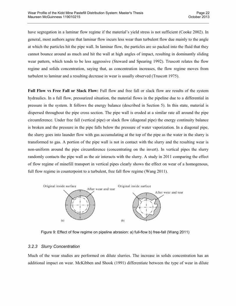
Full Flow vs Free Fall or Slack Flow: Full flow and free fall or slack flow are results of the system
hydraulics. In a full flow, pressurized situation, the material flows in the pipeline due to a differential in
pressure in the system. It follows the energy balance (described in Section 5). In this state, material is
dispersed throughout the pipe cross section. The pipe wall is eroded at a similar rate all around the pipe
circumference. Under free fall (vertical pipe) or slack flow (diagonal pipe) the energy continuity balance
is broken and the pressure in the pipe falls below the pressure of water vaporization. In a diagonal pipe,
the slurry goes into launder flow with gas accumulating at the top of the pipe as the water in the slurry is
transformed to gas. A portion of the pipe wall is not in contact with the slurry and the resulting wear is
non-uniform around the pipe circumference (concentrating on the invert). In vertical pipes the slurry
randomly contacts the pipe wall as the air interacts with the slurry. A study in 2011 comparing the effect
of flow regime of minefill transport in vertical pipes clearly shows the effect on wear of a homogenous,
full flow regime in counterpoint to a turbulent, free fall flow regime (Wang 2011).
Figure 9: Effect of flow regime on pipeline abrasion: a) full-flow b) free-fall (Wang 2011)
3.2.3 Slurry Concentration
Much of the wear studies are performed on dilute slurries. The increase in solids concentration has an
additional impact on wear. McKibben and Shook (1991) differentiate between the type of wear in dilute
Wear Profile of the Kidd Mine Pastefill Distribution System: Master's Thesis Page 23 Maureen McGuinness 119010215 October 2013
and dense slurry flows. Dilute slurry flows3 have wear that is governed by particle – wall interactions and
are influenced by fluid forces. They explain that, “as the concentration of the slurry increases, particle-
particle interactions become more important”, causing an additional source of wear from collisions
between particles causing random impacts with the pipe wall (McKibben and Shook 1991). Steward and
Spearing (1992) show in their study that increased relative density results in the decrease in wear. They
state that the dependency of the exponent n (in the wear relationship W=kVn) on density supports the
theory of the Particle Mean Free Path (discussed by Bain and Bonnington in their 1970 paper) being a
factor in wear, as particles in low density slurries can move around freely and build up energy which then
is expended by the removal of material from the pipe wall. At high densities, the particles cannot move
around freely and their energy is dissipated by hitting other particles rather than the pipe wall (Steward
and Spearing 1992). Inferred from this is that there exists a limiting concentration beyond which the
addition of more particles does not increase wear because these particles are not able to enter into contact
with the pipe wall.
A 2011 study on the effect of slurry concentration and coarse abrasive types on wear of a hard metal
showed a direct relationship between slurry concentration and wear for slurries between 5-40% solids
(Rong, Peng et al. 2011). This suggests that 40% mass solids is still in the range where concentration
affects wear – this corresponds to the 15% volume concentrations cited by Jacobs (1984). Patil also
found, in general, a linear relationship between increasing concentration and wear for slurries at 30-40%
solids (Patil, Deore et al. 2011). In fact, for the number of studies performed on the effect of
concentration on wear, very few were done at high concentrations (over 70% solids or 40% volume).
This is primarily because most of the slurries dealt with until now have had lower concentrations. The
advent of high slurry density or paste is relatively new. In a report in 1992, Steward and Spearing state
that:
“Little work has been carried out on wear in pipelines transporting classified tailings at
volume concentrations between 36 and 46 per cent” (Steward and Spearing 1992)
In 2011, Patil’s research examined the effect of concentration with varying angles of impingement. In
general, these results showed increasing wear with concentration but, again, the concentration range did
not exceed a 40% solid concentration. There were some angles of impact at which, at higher
concentrations, the wear rate seemed to plateau (Patil, Deore et al. 2011). One explanation for this plateau
3 Defined by McKibben and Shook as a slurry with % solids by volume less than 5%

Wear Profile of the Kidd Mine Pastefill Distribution System: Master's Thesis Page 24 Maureen McGuinness 119010215 October 2013
in wear rate may be that increasing the solids concentration changes the wear pattern of the slurry. For
example, increasing the slurry concentration has been shown to unify the wear in the pipe by reducing the
wear from settling particles scraping along the pipe invert. Increasing slurry concentration was shown to
decrease the wear even more (Jvarsheishvili 1982), though the maximum concentration used was not
clear in this report. The wear relationship at higher concentration is an area that needs to be researched
further.
3.2.4 Particle Size
Along with velocity and volume concentration, particle size is an important factor in mechanical abrasive
wear (Shou 2007). Wear was shown to increase linearly as the mean particle size of emery slurry was
increase from 0.015mm to 1.5mm (Jacobs and James 1984). Another study of particle size and angularity
effect on wear shows that the wear rate, with the effect of particle sharpness removed, increases as the
d90 (or the coarseness) of the slurry increases (Steward and Spearing 1993). Similarly, another study
showed an exponential relationship between particle size and wear for most impact angles except for a 45
degree angle of impingement which was linear (Patil, Deore et al. 2011). Other studies have isolated
particular particle size fractions, to examine their individual effect on wear. In a rubber wheel wear test
contacting alumina particles with various types of steel, it was seen that wear rate peaked at a particle size
of 0.125 mm (Chacon-Nava, Martinez-Villafañe et al. 2010) when a range of 50 – 560 μm particles was
evaluated. This result seems to contradict the findings of the whole flow studies mentioned before which
found a linear relationship between an increase of mean particle size and wear rate.
Shou’s in-situ pipe wear measurements showed a different wear pattern between fine slurries and
medium-course slurries. Fine slurries were shown to wear equally across the circumference of the
pipeline while the slurry with coarse particles showed a preferential wear at the invert. Analysis of these
results showed that the dominant wear mode for the finer slurries was corrosion with little abrasion while
the coarse slurry pipeline showed predominantly abrasive wear (Shou 2007).
In all, this is an area with many and often conflicting theories. It is not clear whether an increase of
particle size increases the wear rate or not. This may indicate that there is another factor that is masking
the effect of particle size on wear. While size might be a factor in material removal from the pipe wall due
to the inertia capacity of larger particles, it may not be as important as another property closely associated
with particles size: particle shape.
Wear Profile of the Kidd Mine Pastefill Distribution System: Master's Thesis Page 25 Maureen McGuinness 119010215 October 2013
3.2.5 Particle Shape
It is intuitive that a sharp, pointy particle will have a greater chance of removing pipe wall material than a
round, smooth particle. Several researchers have tried to put a quantitative value on the effect of particle
sharpness on wear. Historically, particle shape characterization has been only qualitative with shape being
described verbally (Davis and Dexter 1972, Swanson and Vetter 1985). These researchers both stress the
importance of the ability to quantify the particle shape instead of using qualitative measurements.
Even though methods do exist to assign a numerical value to a particle’s shape, this is an area that is still
largely qualitative. Of all the factors which affect wear, shape is often cited as an afterthought and with
little technical justification except that it makes sense that it is a factor in wear. With the use of image
analysis in most of the techniques this shape characterization is readily assessable to industry and
researchers. Many particle size analyzers, such as Melvern, offer shape analyzing capability and the
models such as SQP are already incorporated into the data interpretation. This permits the factor of shape
to take a more prominent place in the factors considered for wear. There is evidence that this change is
happening. Rong et al refers to the SPQ value of the particles in his work on the effect of particle
sharpness and slurry concentration on wear (Rong, Peng et al. 2011).
With the use of higher concentration slurries, the interactions of the particles with the pipe wall are more
numerous, even if the type of interaction is predominantly gentler with sliding instead of impingement.
This higher frequency of impact has the potential to increase the importance of particle shape on the wear
rate. This could explain the contradiction seen in the research on the effect of concentration on wear.
While it is generally agreed that a higher concentration results in lower wear or a plateauing of the wear
rate, some studies have had the opposite result: increased wear at higher concentrations. The
differentiating factor may be the particle shape.
3.2.6 Corrosion
Budinski’s definition of erosion-corrosion states that there is a synergy between erosion and corrosion in
which each mode of wear promotes the other, often resulting in higher overall wear than the two
individual modes would normally produce as the slurry particles scour the oxide layer off, perpetuating
the corrosion (Budinski 2007). Corrosion is not generally the first factor that comes to mind when
thinking about wear because it is a chemical phenomenon instead of a mechanical cause of pipe
deterioration. However, the synergy effect of corrosion on erosion makes this an element that should be

Wear Profile of the Kidd Mine Pastefill Distribution System: Master's Thesis Page 26 Maureen McGuinness 119010215 October 2013
examined early on in the mode identification stage, if for no other reason than to eliminate it from the
equation.
Authors argue that corrosion comes into play in wear more often than expected as it accelerates the wear
process. Truscott asserts that:
“the most common type of attack in slurry systems is ‘erosion-corrosion’, where
the rate of corrosion is accelerated by scouring of the surface and removal of
protective oxide or scale films by the impacting solids”(Truscott 1979).
In a study done on wear in nuclear pipelines, it is proposed that the start-up and shutdown modes of the
operation sequence contribute significantly to the overall wear of the pipe element even though they only
constitute around 5% of the life cycle of the pipe (Lovchev 2009). Steward concurs, stating that corrosion
is a problem in South African gold mine minefill systems and cites the high oxygen content and high acid
levels of the flush water as a major contributor to this problem (Steward and Spearing 1992).
Gandhi cites dissolved oxygen as the key factor in pipeline corrosion. As the dissolved oxygen is
depleted, the corrosion rates decrease. Relating this to pipeline slurry systems, he expects higher
corrosion at the start, tapering off along the pipeline as the oxygen levels drop (Gandhi, Ricks et al.
1975). An interesting inverse phenomenon to this oxygen – corrosion relationship is that there is an
oxygen threshold above which the corrosion rate levels off (Cooke, Johnson et al. 2000). This would
mean that slurry pipeline with higher dissolved oxygen would experience the same corrosion rate but the
corrosion would extend further down the pipe system as the higher oxygen levels take longer to be
consumed.
3.3 Summary
This literature review has revealed several points relevant to the study of the Kidd Mine pastefill
distribution system.
The type of wear can be considered erosive since paste is a mixture of solids and water.
The two main subgroups of erosion are slurry wear and corrosion wear.
Slurry wear can include sliding wear and impact wear depending on the angle that the
particles come in contact with the pipe wall.
There are many factors involved in wear and all are interdependent.
Wear Profile of the Kidd Mine Pastefill Distribution System: Master's Thesis Page 27 Maureen McGuinness 119010215 October 2013
Wear is not a parameter of slurry or of the pipe material. It is a result of the overall wear
system which includes the pipe, the material transported and the flow regime.
The dominant factor in wear is considered to be velocity.
Other key wear factors are slurry concentration, corrosion, particle shape and size.
Because most slurry transport is done at low slurry concentration, there is little literature
about pipe wear involving high density slurries, such as pastefill.
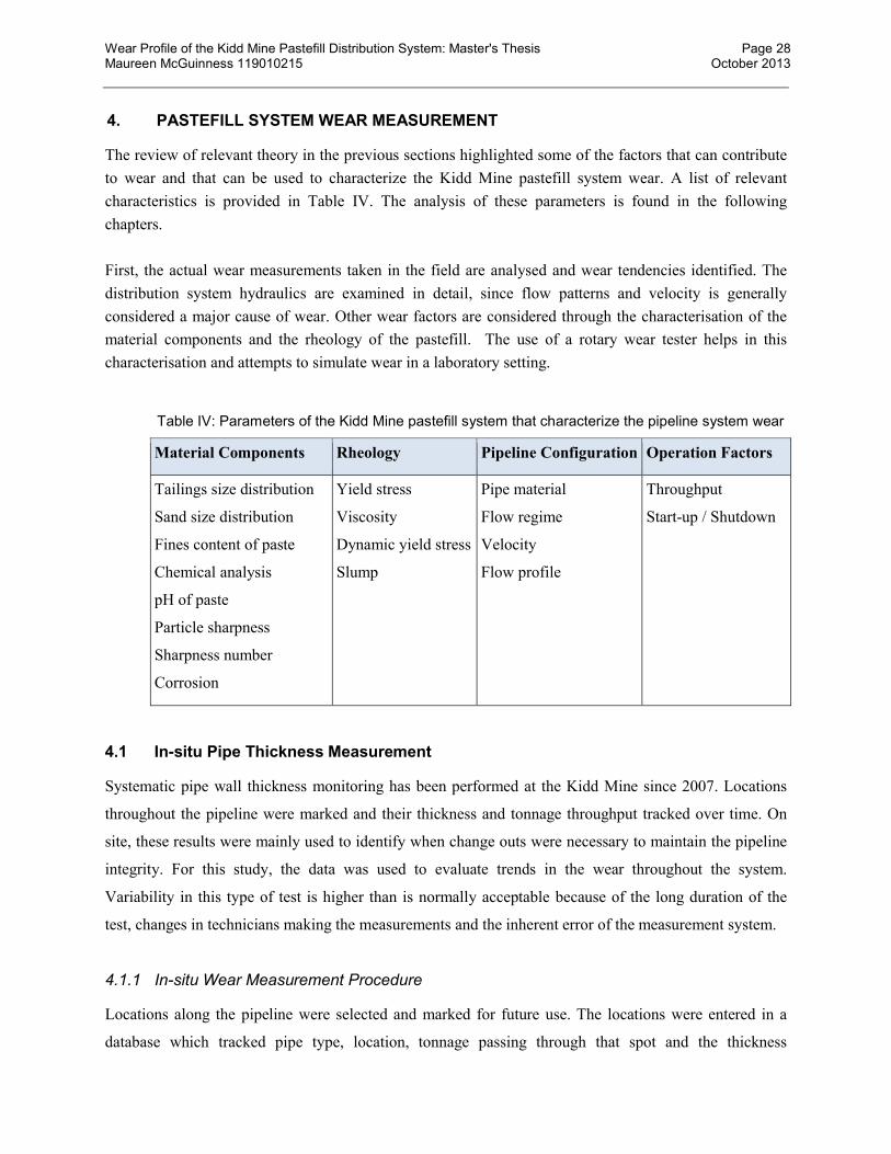
Wear Profile of the Kidd Mine Pastefill Distribution System: Master's Thesis Page 28 Maureen McGuinness 119010215 October 2013
4. PASTEFILL SYSTEM WEAR MEASUREMENT
The review of relevant theory in the previous sections highlighted some of the factors that can contribute
to wear and that can be used to characterize the Kidd Mine pastefill system wear. A list of relevant
characteristics is provided in Table IV. The analysis of these parameters is found in the following
chapters.
First, the actual wear measurements taken in the field are analysed and wear tendencies identified. The
distribution system hydraulics are examined in detail, since flow patterns and velocity is generally
considered a major cause of wear. Other wear factors are considered through the characterisation of the
material components and the rheology of the pastefill. The use of a rotary wear tester helps in this
characterisation and attempts to simulate wear in a laboratory setting.
Table IV: Parameters of the Kidd Mine pastefill system that characterize the pipeline system wear
Material Components Rheology Pipeline Configuration Operation Factors
Tailings size distribution
Sand size distribution
Fines content of paste
Chemical analysis
pH of paste
Particle sharpness
Sharpness number
Corrosion
Yield stress
Viscosity
Dynamic yield stress
Slump
Pipe material
Flow regime
Velocity
Flow profile
Throughput
Start-up / Shutdown
4.1 In-situ Pipe Thickness Measurement
Systematic pipe wall thickness monitoring has been performed at the Kidd Mine since 2007. Locations
throughout the pipeline were marked and their thickness and tonnage throughput tracked over time. On
site, these results were mainly used to identify when change outs were necessary to maintain the pipeline
integrity. For this study, the data was used to evaluate trends in the wear throughout the system.
Variability in this type of test is higher than is normally acceptable because of the long duration of the
test, changes in technicians making the measurements and the inherent error of the measurement system.
4.1.1 In-situ Wear Measurement Procedure
Locations along the pipeline were selected and marked for future use. The locations were entered in a
database which tracked pipe type, location, tonnage passing through that spot and the thickness
Wear Profile of the Kidd Mine Pastefill Distribution System: Master's Thesis Page 29 Maureen McGuinness 119010215 October 2013
measurements by date. Pipeline thickness measurement was performed approximately every three to four
months.
For each location on the pipeline, the pipe wall thickness was measured using a hand held PocketMIKE
ultrasonic gauge manufactured by General Electric Company. Pooled measurements (average of the three
readings of the same location) are used to minimize variation due to surface imperfections on the pipe and
operator error when placing the sensor on the pipe.
4.1.2 Wear Data Set Creation
For the study analysis, only pipe wall thickness data which met certain criteria was included in the final
wear data set. This eliminated a large portion of the data but made it possible to calculate wear rates for
all the measurements retained. The criteria for a measurement to be retained were as follows:
There must have been another measurement of the same location performed in the next round of
testing on the same pipe so that a difference in tonnage and thickness were known. If the pipe
was changed out in between tests, the tonnage and wear loss in that period were not included in
the final data set.
If the thickness of the pipe increased between measurements, the wear gain was not included in
the data set, as it could indicate a pipe change out had taken place or an erroneous measurement
had been made. Material accumulation was not considered to be the reason for the increase in
thickness because paste build-up in the pipe was not common in this system and the thickness
gauge would not usually measure an accumulation since it is another medium.
If the wear reading exceeded the actual thickness of the pipe, the data was not included in the data
set. This mainly eliminated poor readings due to surface imperfections and operator error.
Wear rates were excluded if they exceeded the estimated wear rate based on actual change-out
rate seen for any pipe in the system (1.5mm/100kt) by more than double.
Once the elimination of erroneous data was completed, the data set was further refined to only include
locations with multiple readings.
Only measurement days with four or more valid points on the same level were retained.
Once these criteria had been met, only wear location sites with four or more readings over the life
of the mine were retained.

Wear Profile of the Kidd Mine Pastefill Distribution System: Master's Thesis Page 30 Maureen McGuinness 119010215 October 2013
This resulted in 140 data points being retained in the wear rate data set. They span the life of the pastefill
system, from 2005 to 2010, and represent all the major pastefill loop levels from 1600 down to 5600
level. The points are distributed evenly over the levels with 10 to 20 readings per level. The data set
covers the life of the pastefill plant from 2005 to 2010, but two years (2008 and 2010) are under-
represented. The data distribution is presented in Table V.
Table V: Wear rate data set distribution
Number of Readings by Level Number of Readings by Year
Level 1600 10 2005 18
Level 2000 20 2006 15
Level 2400 15 2007 61
Level 2800 16 2008 7
Level 3800 23 2009 30
Level 4600 20 2010 9
Level 5200 16 TOTAL 140
Level 5600 20
TOTAL 140
4.2 Wear Data Analysis
4.2.1 Overall Wear Rate
Using the wear rate data set produced, the mean wear rate is calculated to be 0.60 mm/100kt of paste
throughput with a 95% confidence interval of 0.53 to 0.66 and a standard deviation of 0.39 mm/100kt
(confidence interval 0.35 to 0.44). This is a wide standard deviation as shown in Figure 10.
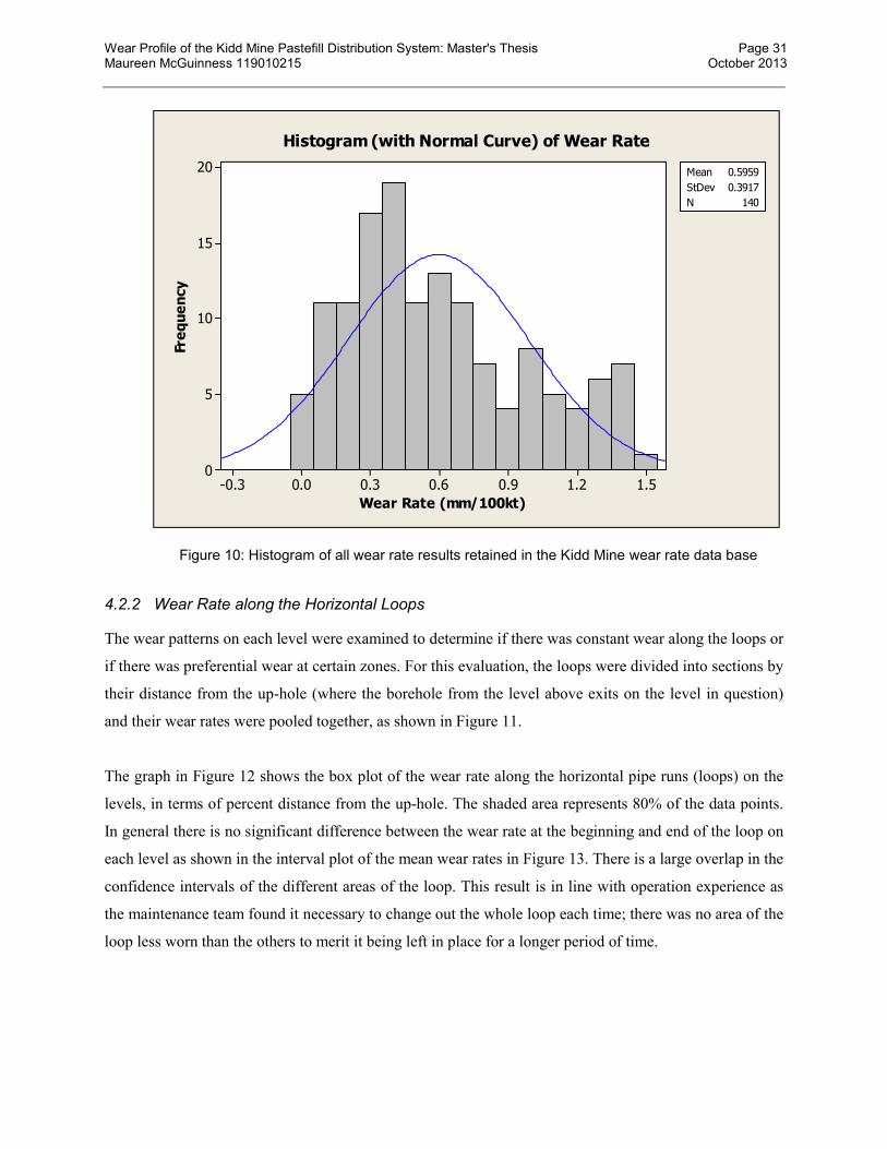
Wear Profile of the Kidd Mine Pastefill Distribution System: Master's Thesis Page 31 Maureen McGuinness 119010215 October 2013
Figure 10: Histogram of all wear rate results retained in the Kidd Mine wear rate data base
4.2.2 Wear Rate along the Horizontal Loops
The wear patterns on each level were examined to determine if there was constant wear along the loops or
if there was preferential wear at certain zones. For this evaluation, the loops were divided into sections by
their distance from the up-hole (where the borehole from the level above exits on the level in question)
and their wear rates were pooled together, as shown in Figure 11.
The graph in Figure 12 shows the box plot of the wear rate along the horizontal pipe runs (loops) on the
levels, in terms of percent distance from the up-hole. The shaded area represents 80% of the data points.
In general there is no significant difference between the wear rate at the beginning and end of the loop on
each level as shown in the interval plot of the mean wear rates in Figure 13. There is a large overlap in the
confidence intervals of the different areas of the loop. This result is in line with operation experience as
the maintenance team found it necessary to change out the whole loop each time; there was no area of the
loop less worn than the others to merit it being left in place for a longer period of time.
1.51.20.90.60.30.0-0.3
20
15
10
5
0
Wear Rate (mm/100kt)
Fre
qu
en
cy
Mean 0.5959
StDev 0.3917
N 140
Histogram (with Normal Curve) of Wear Rate

Wear Profile of the Kidd Mine Pastefill Distribution System: Master's Thesis Page 32 Maureen McGuinness 119010215 October 2013
Figure 11: Schematic of pooling groups by distance from up-hole
Figure 12: Average wear rate vs % distance along the loop
80-100%60-80%40-60%20-40%0-20%
1.6
1.4
1.2
1.0
0.8
0.6
0.4
0.2
0.0
Distance from uphole (% range)
mm
/1
00
kt
Boxplot of Wear Rate vs Distance from Uphole

Wear Profile of the Kidd Mine Pastefill Distribution System: Master's Thesis Page 33 Maureen McGuinness 119010215 October 2013
Figure 13: Interval plot of average wear rate vs % distance from uphole
This technique compared the wear rate over distance in terms of percentage which normalized the loops
independent of their actual length. This approach simplified comparison among levels of differing lengths
but may have obscured some trends that are a function of total length travelled.
A second analysis was done that examined the effect of absolute pipe length on the wear rate by
examining the wear rate along each level individually. The results are shown in Figure 14. No systematic
wear pattern along the horizontal runs is evident. In some loops the wear decreases with distance along
the loop and in others it increases.
80-100%60-80%40-60%20-40%0-20%
1.1
1.0
0.9
0.8
0.7
0.6
0.5
0.4
0.3
Distance from uphole (% range)
We
ar
Ra
te (
mm
/1
00
kt)
95% CI for the Mean
Interval Plot of Wear Rate vs Distance from Uphole

Wear Profile of the Kidd Mine Pastefill Distribution System: Master's Thesis Page 34 Maureen McGuinness 119010215 October 2013
Figure 14: Examination by level of wear rate vs distance along the horizontal loop
4.2.3 Wear vs Distance from Surface
The next relationship examined was the trend of wear throughout the piping system as a whole. The
average wear rate per level was compared against the pipeline distance to that level from the surface. In
Section 4.2.2, the individual levels were examined on a local scale for wear trends and it was concluded
that wear rates were essentially stable throughout the level. Since the levels are short relative to long
vertical distances of the boreholes, the wear data was grouped together by level for the overall system
evaluation.
The box plot in Figure 15 indicates that the average wear rates seem to drop as the level is located further
away from surface but the intervals for the means do overlap making the average not significantly
different, for most of the levels. The interval plot of the pooled wear rates by level is shown in Figure 16.
1.6
0.8
0.0
100500
100500
1.6
0.8
0.0
100500
1.6
0.8
0.0
1600
Distance from uphole (m)
We
ar
Ra
te (
mm
/1
00
kt)
2000 2400
2800 3800 4600
5200 5600
13-Dec-05
1-May-06
11-Mar-07
6-Jun-07
2-Dec-07
16-Oct-08
26-May-09
17-Sep-09
17-Mar-10
DATE
Panel variable: Level
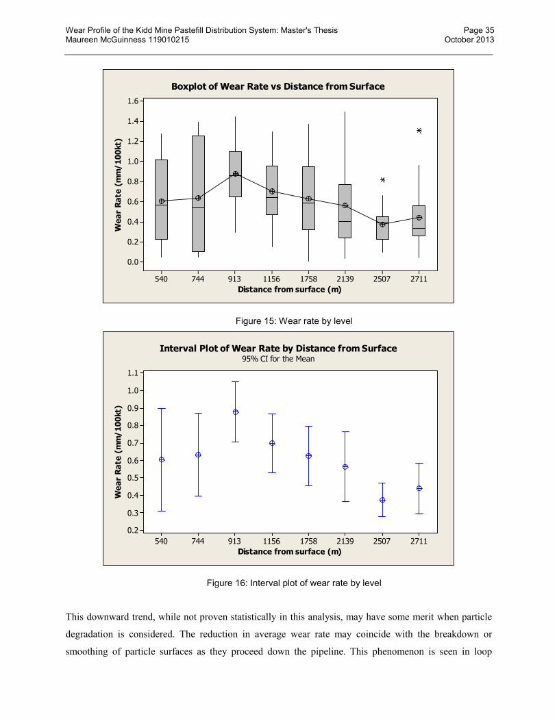
Wear Profile of the Kidd Mine Pastefill Distribution System: Master's Thesis Page 35 Maureen McGuinness 119010215 October 2013
Figure 15: Wear rate by level
Figure 16: Interval plot of wear rate by level
This downward trend, while not proven statistically in this analysis, may have some merit when particle
degradation is considered. The reduction in average wear rate may coincide with the breakdown or
smoothing of particle surfaces as they proceed down the pipeline. This phenomenon is seen in loop
27112507213917581156913744540
1.6
1.4
1.2
1.0
0.8
0.6
0.4
0.2
0.0
Distance from surface (m)
We
ar
Ra
te (
mm
/1
00
kt)
Boxplot of Wear Rate vs Distance from Surface
27112507213917581156913744540
1.1
1.0
0.9
0.8
0.7
0.6
0.5
0.4
0.3
0.2
Distance from surface (m)
We
ar
Ra
te (
mm
/1
00
kt)
95% CI for the Mean
Interval Plot of Wear Rate by Distance from Surface
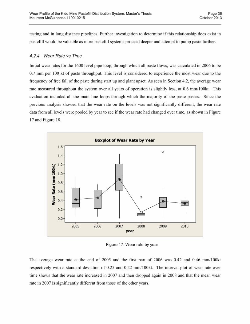
Wear Profile of the Kidd Mine Pastefill Distribution System: Master's Thesis Page 36 Maureen McGuinness 119010215 October 2013
testing and in long distance pipelines. Further investigation to determine if this relationship does exist in
pastefill would be valuable as more pastefill systems proceed deeper and attempt to pump paste further.
4.2.4 Wear Rate vs Time
Initial wear rates for the 1600 level pipe loop, through which all paste flows, was calculated in 2006 to be
0.7 mm per 100 kt of paste throughput. This level is considered to experience the most wear due to the
frequency of free fall of the paste during start up and plant upset. As seen in Section 4.2, the average wear
rate measured throughout the system over all years of operation is slightly less, at 0.6 mm/100kt. This
evaluation included all the main line loops through which the majority of the paste passes. Since the
previous analysis showed that the wear rate on the levels was not significantly different, the wear rate
data from all levels were pooled by year to see if the wear rate had changed over time, as shown in Figure
17 and Figure 18.
Figure 17: Wear rate by year
The average wear rate at the end of 2005 and the first part of 2006 was 0.42 and 0.46 mm/100kt
respectively with a standard deviation of 0.25 and 0.22 mm/100kt. The interval plot of wear rate over
time shows that the wear rate increased in 2007 and then dropped again in 2008 and that the mean wear
rate in 2007 is significantly different from those of the other years.
201020092008200720062005
1.6
1.4
1.2
1.0
0.8
0.6
0.4
0.2
0.0
year
We
ar
Ra
te (
mm
/1
00
kt)
Boxplot of Wear Rate by Year
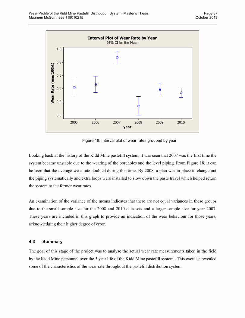
Wear Profile of the Kidd Mine Pastefill Distribution System: Master's Thesis Page 37 Maureen McGuinness 119010215 October 2013
Figure 18: Interval plot of wear rates grouped by year
Looking back at the history of the Kidd Mine pastefill system, it was seen that 2007 was the first time the
system became unstable due to the wearing of the boreholes and the level piping. From Figure 18, it can
be seen that the average wear rate doubled during this time. By 2008, a plan was in place to change out
the piping systematically and extra loops were installed to slow down the paste travel which helped return
the system to the former wear rates.
An examination of the variance of the means indicates that there are not equal variances in these groups
due to the small sample size for the 2008 and 2010 data sets and a larger sample size for year 2007.
These years are included in this graph to provide an indication of the wear behaviour for those years,
acknowledging their higher degree of error.
4.3 Summary
The goal of this stage of the project was to analyse the actual wear rate measurements taken in the field
by the Kidd Mine personnel over the 5 year life of the Kidd Mine pastefill system. This exercise revealed
some of the characteristics of the wear rate throughout the pastefill distribution system.
201020092008200720062005
1.0
0.8
0.6
0.4
0.2
0.0
year
We
ar
Ra
te (
mm
/1
00
kt)
95% CI for the Mean
Interval Plot of Wear Rate by Year

Wear Profile of the Kidd Mine Pastefill Distribution System: Master's Thesis Page 38 Maureen McGuinness 119010215 October 2013
The mean wear rate is calculated to be 0.60 mm/100kt of paste throughput with a 95%
confidence interval of 0.53 to 0.66 mm/100kt.
The wear rate originally measured on the first paste loop (1600 level) in 2006 falls within
the predicted wear rate range of the whole system.
No significant difference was seen between the wear measurements along the horizontal
loop runs.
There was an indication of decreasing average wear with increasing travel distance but
the relationship was not proven statistically. Further investigation into this relationship is
warranted.
Wear rates did change over the years. The rate was seen to increase during periods of
instability in the system which reflects times when many boreholes were in free fall
resulting in higher flow rates on the system.
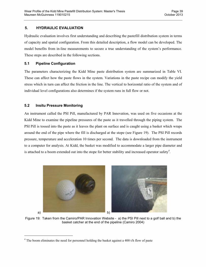
Wear Profile of the Kidd Mine Pastefill Distribution System: Master's Thesis Page 39 Maureen McGuinness 119010215 October 2013
5. HYDRAULIC EVALUATION
Hydraulic evaluation involves first understanding and describing the pastefill distribution system in terms
of capacity and spatial configuration. From this detailed description, a flow model can be developed. The
model benefits from in-line measurements to secure a true understanding of the system’s performance.
These steps are described in the following sections.
5.1 Pipeline Configuration
The parameters characterizing the Kidd Mine paste distribution system are summarized in Table VI.
These can affect how the paste flows in the system. Variations in the paste recipe can modify the yield
stress which in turn can affect the friction in the line. The vertical to horizontal ratio of the system and of
individual level configurations also determines if the system runs in full flow or not.
5.2 Insitu Pressure Monitoring
An instrument called the PSI Pill, manufactured by PAR Innovation, was used on five occasions at the
Kidd Mine to examine the pipeline pressures of the paste as it travelled through the piping system. The
PSI Pill is tossed into the paste as it leaves the plant on surface and is caught using a basket which wraps
around the end of the pipe where the fill is discharged at the stope (see Figure 19). The PSI Pill records
pressure, temperature and acceleration 10 times per second. The data is downloaded from the instrument
to a computer for analysis. At Kidd, the basket was modified to accommodate a larger pipe diameter and
is attached to a boom extended out into the stope for better stability and increased operator safety4.
a) b)
Figure 19: Taken from the Camiro/PAR Innovation Website - a) the PSI Pill next to a golf ball and b) the basket catcher at the end of the pipeline (Camiro 2004)
4 The boom eliminates the need for personnel holding the basket against a 400 t/h flow of paste
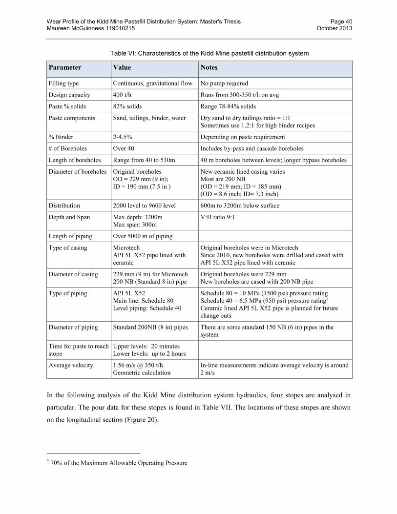
Wear Profile of the Kidd Mine Pastefill Distribution System: Master's Thesis Page 40 Maureen McGuinness 119010215 October 2013
Table VI: Characteristics of the Kidd Mine pastefill distribution system
Parameter Value Notes
Filling type Continuous, gravitational flow No pump required
Design capacity 400 t/h Runs from 300-350 t/h on avg
Paste % solids 82% solids Range 78-84% solids
Paste components Sand, tailings, binder, water Dry sand to dry tailings ratio = 1:1 Sometimes use 1.2:1 for high binder recipes
% Binder 2-4.5% Depending on paste requirement
# of Boreholes Over 40 Includes by-pass and cascade boreholes
Length of boreholes Range from 40 to 530m 40 m boreholes between levels; longer bypass boreholes
Diameter of boreholes Original boreholes OD = 229 mm (9 in); ID = 190 mm (7.5 in )
New ceramic lined casing varies Most are 200 NB (OD = 219 mm; ID = 185 mm) (OD = 8.6 inch; ID= 7.3 inch)
Distribution 2000 level to 9600 level 600m to 3200m below surface
Depth and Span Max depth: 3200m Max span: 300m
V:H ratio 9:1
Length of piping Over 5000 m of piping
Type of casing Microtech API 5L X52 pipe lined with ceramic
Original boreholes were in Microtech Since 2010, new boreholes were drilled and cased with API 5L X52 pipe lined with ceramic
Diameter of casing 229 mm (9 in) for Microtech 200 NB (Standard 8 in) pipe
Original boreholes were 229 mm New boreholes are cased with 200 NB pipe
Type of piping API 5L X52 Main line: Schedule 80 Level piping: Schedule 40
Schedule 80 = 10 MPa (1500 psi) pressure rating Schedule 40 = 6.5 MPa (950 psi) pressure rating5 Ceramic lined API 5L X52 pipe is planned for future change outs
Diameter of piping Standard 200NB (8 in) pipes There are some standard 150 NB (6 in) pipes in the system
Time for paste to reach stope
Upper levels: 20 minutes Lower levels: up to 2 hours
Average velocity 1.56 m/s @ 350 t/h Geometric calculation
In-line measurements indicate average velocity is around 2 m/s
In the following analysis of the Kidd Mine distribution system hydraulics, four stopes are analysed in
particular. The pour data for these stopes is found in Table VII. The locations of these stopes are shown
on the longitudinal section (Figure 20).
5 70% of the Maximum Allowable Operating Pressure

Wear Profile of the Kidd Mine Pastefill Distribution System: Master's Thesis Page 41 Maureen McGuinness 119010215 October 2013
Figure 20: Location of PSI Pill test stopes and examples of raw PSI Pill pressure data charts
Table VII: Pour data for the PSI Pill tests
63-822-ST 75-905-ST 66-GW1-ST 66-745-ST
Date of test Jan 13, 2005 Feb 13, 2005 May 15, 2006 July 7, 2007
Paste Throughput to date (t) 121925 179927 1097312 2581680
Total pipe route length (m) 2780 3640 3284 3254
Elevation change (m) -1817 -2263 -1962 -1962
Horizontal on last level (m) 260 110 270 260
Slump 7.0 6.5 6.25 5.25
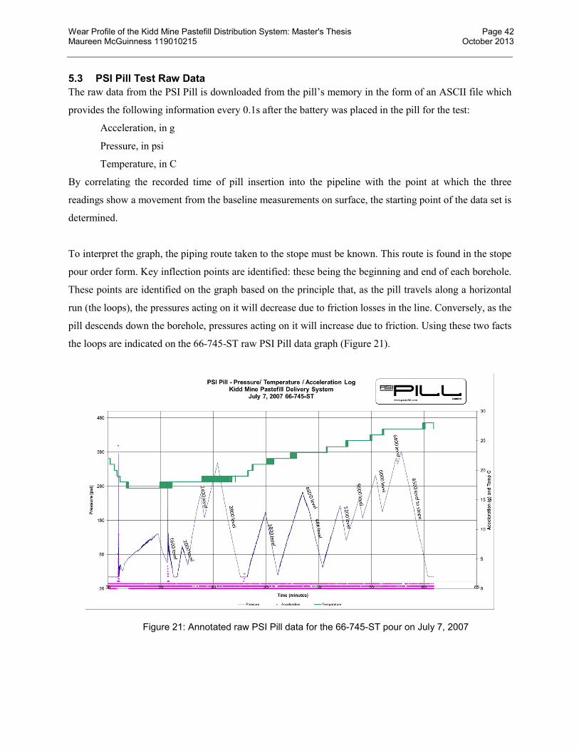
Wear Profile of the Kidd Mine Pastefill Distribution System: Master's Thesis Page 42 Maureen McGuinness 119010215 October 2013
5.3 PSI Pill Test Raw Data
The raw data from the PSI Pill is downloaded from the pill’s memory in the form of an ASCII file which
provides the following information every 0.1s after the battery was placed in the pill for the test:
Acceleration, in g
Pressure, in psi
Temperature, in C
By correlating the recorded time of pill insertion into the pipeline with the point at which the three
readings show a movement from the baseline measurements on surface, the starting point of the data set is
determined.
To interpret the graph, the piping route taken to the stope must be known. This route is found in the stope
pour order form. Key inflection points are identified: these being the beginning and end of each borehole.
These points are identified on the graph based on the principle that, as the pill travels along a horizontal
run (the loops), the pressures acting on it will decrease due to friction losses in the line. Conversely, as the
pill descends down the borehole, pressures acting on it will increase due to friction. Using these two facts
the loops are indicated on the 66-745-ST raw PSI Pill data graph (Figure 21).
Figure 21: Annotated raw PSI Pill data for the 66-745-ST pour on July 7, 2007

Wear Profile of the Kidd Mine Pastefill Distribution System: Master's Thesis Page 43 Maureen McGuinness 119010215 October 2013
Cross-checking with other pipe route knowledge helps confirm the level placement on the graph. In this
case, it is known that the loop piping on level 2800 is extremely long compared to other loops. The
identification of 2800 level data on the graph is confirmed as the pressure loss along this level is much
larger than for the other levels. Another confirmation point is the last level on which the pressures must
go to zero as the pill falls into the stope. Note that the discharge point is located on the 6500 level since
the paste is poured into the 6600 level stope from the level above.
With the key points in the graph identified, the data set is then manipulated into a format in which its data
can be extracted and compared to other stope data, mainly the hydraulic model.
5.4 PSI Pill Data Compilation
A multistep process was used to transform the PSI Pill data into a working data set. The goal of this data
manipulation was to reduce the noise in the data and the quantity of data into a manageable amount that
could be compared to other system data, notably the flow model. The steps involved were:
Pool the data – With 10 readings taken every second, there are over 28000 readings per test
which involved much variation that was insignificant to the test. It was shown that a pool of 90
readings reduced the data considerably and smoothed out the variation.
Zero the data – The data was zeroed at the true start time for each test for better comparison
between tests. Similarly, pressure offsets of the PSI Pill were removed from the data by taking the
pressure at the stope as the zero value.
Identify peaks and valleys – In most cases, the rate of pressure increase with progression down
the boreholes was constant as was the pressure decrease along the horizontal levels. To match the
PSI Pill data to the hydraulic model, the constant rate was used as a means to join the points of
inflection in the pipeline, as shown in Figure 22. This technique must be used cautiously to
ensure it is increasing the value of the data and not diluting out valuable information and
tendencies.
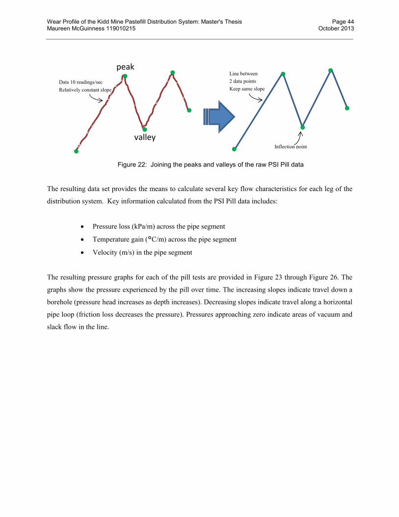
Wear Profile of the Kidd Mine Pastefill Distribution System: Master's Thesis Page 44 Maureen McGuinness 119010215 October 2013
Figure 22: Joining the peaks and valleys of the raw PSI Pill data
The resulting data set provides the means to calculate several key flow characteristics for each leg of the
distribution system. Key information calculated from the PSI Pill data includes:
Pressure loss (kPa/m) across the pipe segment
Temperature gain (°C/m) across the pipe segment
Velocity (m/s) in the pipe segment
The resulting pressure graphs for each of the pill tests are provided in Figure 23 through Figure 26. The
graphs show the pressure experienced by the pill over time. The increasing slopes indicate travel down a
borehole (pressure head increases as depth increases). Decreasing slopes indicate travel along a horizontal
pipe loop (friction loss decreases the pressure). Pressures approaching zero indicate areas of vacuum and
slack flow in the line.
Line between
2 data points
Keep same slope
Data 10 readings/sec
Relatively constant slope
valley
peak
Inflection point
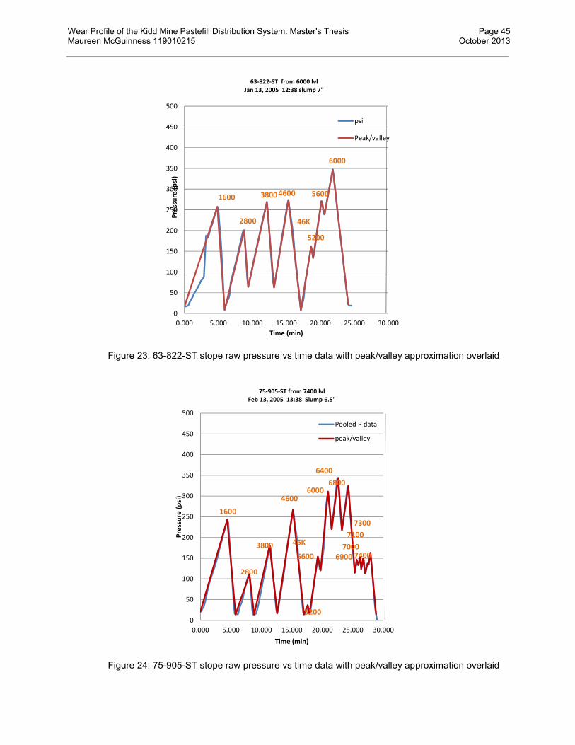
Wear Profile of the Kidd Mine Pastefill Distribution System: Master's Thesis Page 45 Maureen McGuinness 119010215 October 2013
Figure 23: 63-822-ST stope raw pressure vs time data with peak/valley approximation overlaid
Figure 24: 75-905-ST stope raw pressure vs time data with peak/valley approximation overlaid
0
50
100
150
200
250
300
350
400
450
500
0.000 5.000 10.000 15.000 20.000 25.000 30.000
Pre
ssu
re (
psi
)
Time (min)
63-822-ST from 6000 lvlJan 13, 2005 12:38 slump 7"
psi
Peak/valley
1600
2800
3800 4600
46K
5200
5600
6000
0
50
100
150
200
250
300
350
400
450
500
0.000 5.000 10.000 15.000 20.000 25.000 30.000
Pre
ssu
re (
psi
)
Time (min)
75-905-ST from 7400 lvlFeb 13, 2005 13:38 Slump 6.5"
Pooled P data
peak/valley
1600
2800
3800
4600
46K
5200
5600
6000
6400
6800
69007000
7100
7300
7400

Wear Profile of the Kidd Mine Pastefill Distribution System: Master's Thesis Page 46 Maureen McGuinness 119010215 October 2013
Figure 25: 66-GW1-ST stope raw pressure vs time data with peak/valley approximation overlaid
Figure 26: 66-745-ST stope raw pressure vs time data with peak/valley approximation overlaid
0
50
100
150
200
250
300
350
400
450
500
0.000 5.000 10.000 15.000 20.000 25.000 30.000
Pre
ssu
re (
psi
)
Time (min)
66-GW1-ST from 6500 levelMay 15, 2006 16:00 Slump 6.5"
psi #1
peak/valley
1600 2800
3800
4600
46K5200
5600
600061006200
6300
6400
6500
0
50
100
150
200
250
300
350
400
450
500
0.000 5.000 10.000 15.000 20.000 25.000 30.000
Pre
ssu
re (
psi
)
Time (min)
66-745-ST from 6500 levelJuly 7, 2007 23:02 Slump 5.25"
psi
peak/valley
1600 (problem)
2000
2400
2800
3800
4600
46K5200
5600
6000
64006500
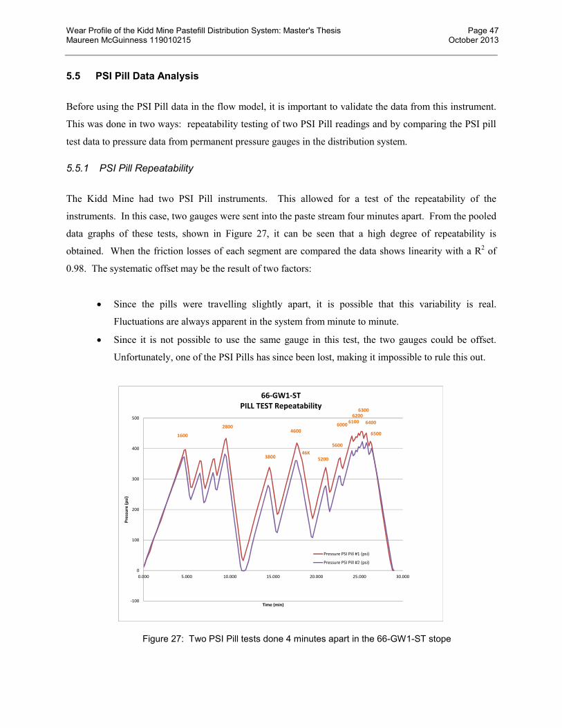
Wear Profile of the Kidd Mine Pastefill Distribution System: Master's Thesis Page 47 Maureen McGuinness 119010215 October 2013
5.5 PSI Pill Data Analysis
Before using the PSI Pill data in the flow model, it is important to validate the data from this instrument.
This was done in two ways: repeatability testing of two PSI Pill readings and by comparing the PSI pill
test data to pressure data from permanent pressure gauges in the distribution system.
5.5.1 PSI Pill Repeatability
The Kidd Mine had two PSI Pill instruments. This allowed for a test of the repeatability of the
instruments. In this case, two gauges were sent into the paste stream four minutes apart. From the pooled
data graphs of these tests, shown in Figure 27, it can be seen that a high degree of repeatability is
obtained. When the friction losses of each segment are compared the data shows linearity with a R2 of
0.98. The systematic offset may be the result of two factors:
Since the pills were travelling slightly apart, it is possible that this variability is real.
Fluctuations are always apparent in the system from minute to minute.
Since it is not possible to use the same gauge in this test, the two gauges could be offset.
Unfortunately, one of the PSI Pills has since been lost, making it impossible to rule this out.
Figure 27: Two PSI Pill tests done 4 minutes apart in the 66-GW1-ST stope
-100
0
100
200
300
400
500
0.000 5.000 10.000 15.000 20.000 25.000 30.000
Pre
ssu
re (
psi
)
Time (min)
66-GW1-ST PILL TEST Repeatability
Pressure PSI Pill #1 (psi)
Pressure PSI Pill #2 (psi)
1600
2800
3800
4600
46K5200
5600
60006100
62006300
6400
6500
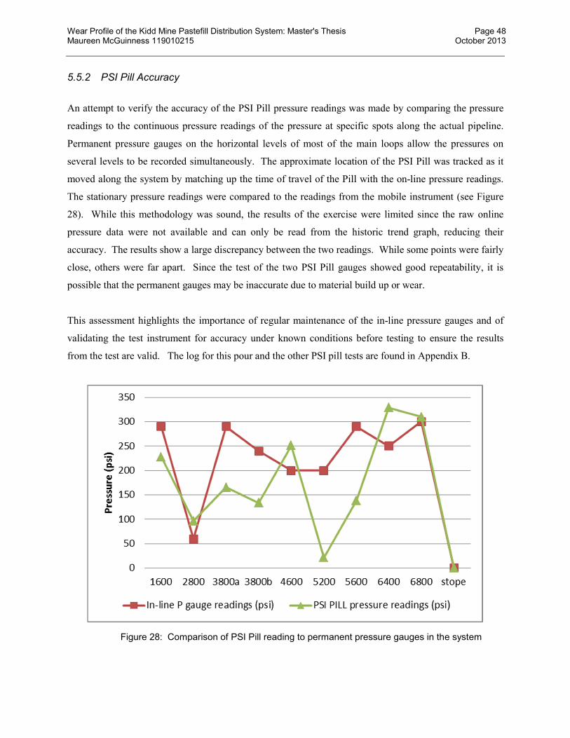
Wear Profile of the Kidd Mine Pastefill Distribution System: Master's Thesis Page 48 Maureen McGuinness 119010215 October 2013
5.5.2 PSI Pill Accuracy
An attempt to verify the accuracy of the PSI Pill pressure readings was made by comparing the pressure
readings to the continuous pressure readings of the pressure at specific spots along the actual pipeline.
Permanent pressure gauges on the horizontal levels of most of the main loops allow the pressures on
several levels to be recorded simultaneously. The approximate location of the PSI Pill was tracked as it
moved along the system by matching up the time of travel of the Pill with the on-line pressure readings.
The stationary pressure readings were compared to the readings from the mobile instrument (see Figure
28). While this methodology was sound, the results of the exercise were limited since the raw online
pressure data were not available and can only be read from the historic trend graph, reducing their
accuracy. The results show a large discrepancy between the two readings. While some points were fairly
close, others were far apart. Since the test of the two PSI Pill gauges showed good repeatability, it is
possible that the permanent gauges may be inaccurate due to material build up or wear.
This assessment highlights the importance of regular maintenance of the in-line pressure gauges and of
validating the test instrument for accuracy under known conditions before testing to ensure the results
from the test are valid. The log for this pour and the other PSI pill tests are found in Appendix B.
Figure 28: Comparison of PSI Pill reading to permanent pressure gauges in the system

Wear Profile of the Kidd Mine Pastefill Distribution System: Master's Thesis Page 49 Maureen McGuinness 119010215 October 2013
5.6 Flow Modeling
The hydraulic model of the Kidd Mine distribution system is derived from first principles, based on the
energy equation. The model mechanics are constant but must be applied to each individual stope, taking
into account the piping configuration to get from surface to the stope and friction loss in the pipeline.
When applying the balance to a section of pipeline, Cooke writes the equation in terms of head, or meters
of slurry, as shown below Cooke (2007):
The following assumptions were used to simplify the equation:
1. The velocity in the line is constant (for the same pipe diameter)
2. The is no external source of energy (no pump)
The hydraulic model is built from the bottom up. This is because there is one point in the system where
the pressure is known without a doubt. At the end of the pipeline as the paste falls into the stope, the
pressure is zero (atmosphere). From this point, the pressures at the other points can be determined by
working back up through the pipeline one section at a time.
Applying this method to the layout example shown in Figure 29, the piping system is divided into two
parts and the pressures at each end of the pipe segment are calculated starting from the bottom segment
which empties into atmosphere.
fp Hg
vz
g
PH
g
vz
g
P
2
221
22
2
121
11
where: v = mean pipeline velocity, m/s g = gravitational acceleration, m/s2 ρ= density, kg/m3 z = elevation, m P = pressure, Pa ∆Hp = head input by pump, m of slurry ∆Hf = friction losses, m of slurry 1,2 subscripts refer to upstream and downstream section respectively
Equation 5-1
fHz
g
Pz
g
P 2
21
1
Equation 5-2
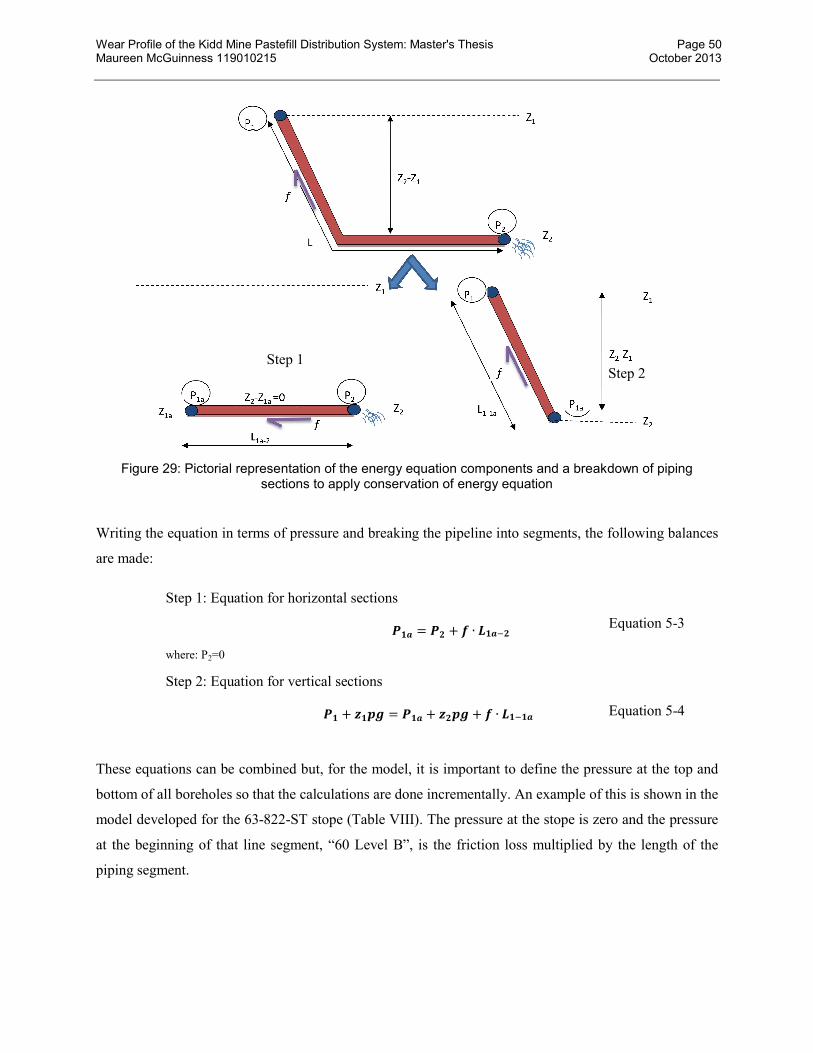
Wear Profile of the Kidd Mine Pastefill Distribution System: Master's Thesis Page 50 Maureen McGuinness 119010215 October 2013
Figure 29: Pictorial representation of the energy equation components and a breakdown of piping sections to apply conservation of energy equation
Writing the equation in terms of pressure and breaking the pipeline into segments, the following balances
are made:
These equations can be combined but, for the model, it is important to define the pressure at the top and
bottom of all boreholes so that the calculations are done incrementally. An example of this is shown in the
model developed for the 63-822-ST stope (Table VIII). The pressure at the stope is zero and the pressure
at the beginning of that line segment, “60 Level B”, is the friction loss multiplied by the length of the
piping segment.
��� = �� + � ∙���� �
Step 1: Equation for horizontal sections
where: P2=0
Equation 5-3
�� + ���� = ��� + ���� + � ∙�����
Step 2: Equation for vertical sections
Equation 5-4
Step 1 Step 2
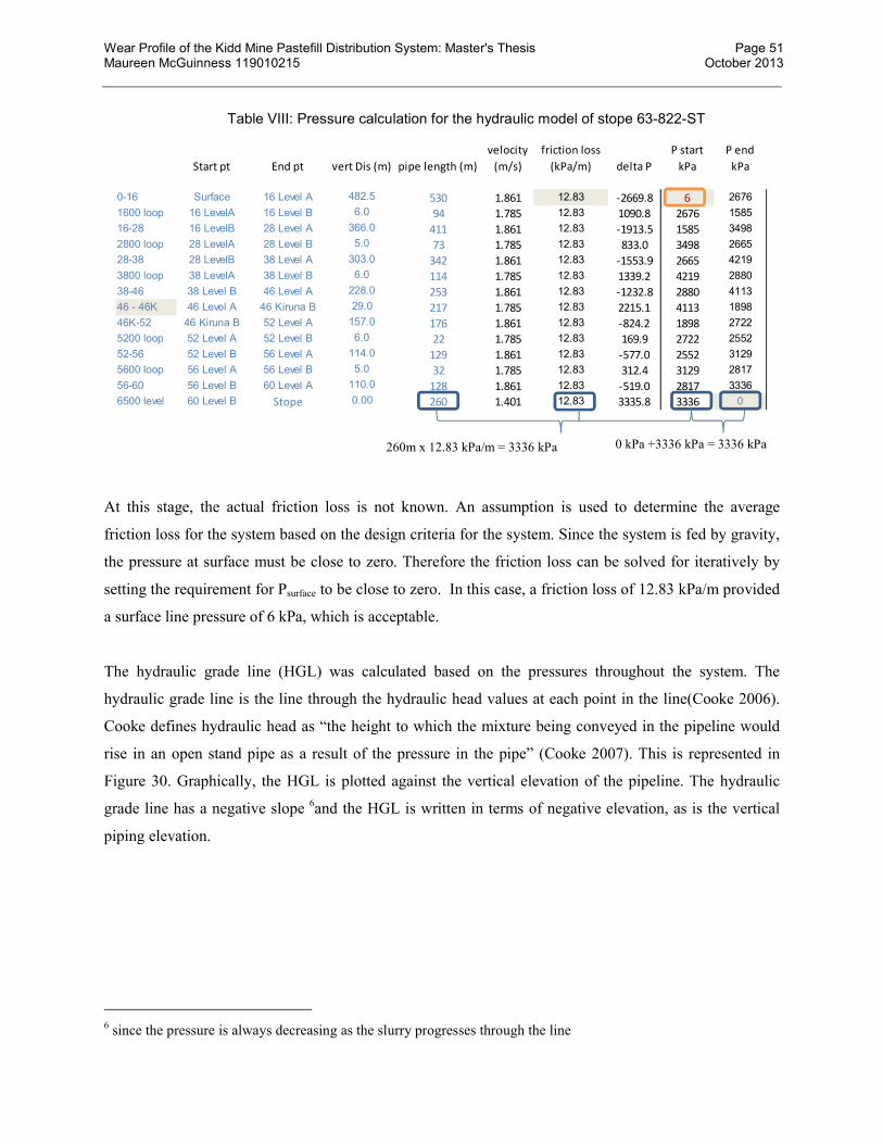
Wear Profile of the Kidd Mine Pastefill Distribution System: Master's Thesis Page 51 Maureen McGuinness 119010215 October 2013
Table VIII: Pressure calculation for the hydraulic model of stope 63-822-ST
At this stage, the actual friction loss is not known. An assumption is used to determine the average
friction loss for the system based on the design criteria for the system. Since the system is fed by gravity,
the pressure at surface must be close to zero. Therefore the friction loss can be solved for iteratively by
setting the requirement for Psurface to be close to zero. In this case, a friction loss of 12.83 kPa/m provided
a surface line pressure of 6 kPa, which is acceptable.
The hydraulic grade line (HGL) was calculated based on the pressures throughout the system. The
hydraulic grade line is the line through the hydraulic head values at each point in the line(Cooke 2006).
Cooke defines hydraulic head as “the height to which the mixture being conveyed in the pipeline would
rise in an open stand pipe as a result of the pressure in the pipe” (Cooke 2007). This is represented in
Figure 30. Graphically, the HGL is plotted against the vertical elevation of the pipeline. The hydraulic
grade line has a negative slope 6and the HGL is written in terms of negative elevation, as is the vertical
piping elevation.
6 since the pressure is always decreasing as the slurry progresses through the line
Start pt End pt vert Dis (m) pipe length (m)
velocity
(m/s)
friction loss
(kPa/m) delta P
P start
kPa
P end
kPa
0-16 Surface 16 Level A 482.5 530 1.861 12.83 -2669.8 6 2676
1600 loop 16 LevelA 16 Level B 6.0 94 1.785 12.83 1090.8 2676 1585
16-28 16 LevelB 28 Level A 366.0 411 1.861 12.83 -1913.5 1585 3498
2800 loop 28 LevelA 28 Level B 5.0 73 1.785 12.83 833.0 3498 2665
28-38 28 LevelB 38 Level A 303.0 342 1.861 12.83 -1553.9 2665 4219
3800 loop 38 LevelA 38 Level B 6.0 114 1.785 12.83 1339.2 4219 2880
38-46 38 Level B 46 Level A 228.0 253 1.861 12.83 -1232.8 2880 4113
46 - 46K 46 Level A 46 Kiruna B 29.0 217 1.785 12.83 2215.1 4113 1898
46K-52 46 Kiruna B 52 Level A 157.0 176 1.861 12.83 -824.2 1898 2722
5200 loop 52 Level A 52 Level B 6.0 22 1.785 12.83 169.9 2722 2552
52-56 52 Level B 56 Level A 114.0 129 1.861 12.83 -577.0 2552 3129
5600 loop 56 Level A 56 Level B 5.0 32 1.785 12.83 312.4 3129 2817
56-60 56 Level B 60 Level A 110.0 128 1.861 12.83 -519.0 2817 3336
6500 level 60 Level B Stope 0.00 260 1.401 12.83 3335.8 3336 0
260m x 12.83 kPa/m = 3336 kPa 0 kPa +3336 kPa = 3336 kPa
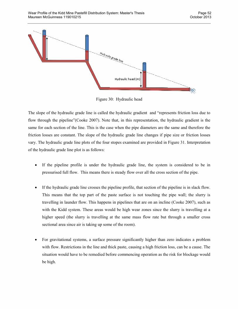
Wear Profile of the Kidd Mine Pastefill Distribution System: Master's Thesis Page 52 Maureen McGuinness 119010215 October 2013
Figure 30: Hydraulic head
The slope of the hydraulic grade line is called the hydraulic gradient and “represents friction loss due to
flow through the pipeline”(Cooke 2007). Note that, in this representation, the hydraulic gradient is the
same for each section of the line. This is the case when the pipe diameters are the same and therefore the
friction losses are constant. The slope of the hydraulic grade line changes if pipe size or friction losses
vary. The hydraulic grade line plots of the four stopes examined are provided in Figure 31. Interpretation
of the hydraulic grade line plot is as follows:
If the pipeline profile is under the hydraulic grade line, the system is considered to be in
pressurised full flow. This means there is steady flow over all the cross section of the pipe.
If the hydraulic grade line crosses the pipeline profile, that section of the pipeline is in slack flow.
This means that the top part of the paste surface is not touching the pipe wall; the slurry is
travelling in launder flow. This happens in pipelines that are on an incline (Cooke 2007), such as
with the Kidd system. These areas would be high wear zones since the slurry is travelling at a
higher speed (the slurry is travelling at the same mass flow rate but through a smaller cross
sectional area since air is taking up some of the room).
For gravitational systems, a surface pressure significantly higher than zero indicates a problem
with flow. Restrictions in the line and thick paste, causing a high friction loss, can be a cause. The
situation would have to be remedied before commencing operation as the risk for blockage would
be high.

Wear Profile of the Kidd Mine Pastefill Distribution System: Master's Thesis Page 53 Maureen McGuinness 119010215 October 2013
Figure 31: Hydraulic models of the four stopes
In the models in Figure 31, there is one point on the 75-905-ST pipeline that is predicted to be in slack
flow (the hydraulic line (HGL) is touching the blue pipeline profile). One reason why this configuration
is susceptible to slack flow is that the horizontal length on the last level is shorter than in the other cases.
This last run has a large effect on the behaviour of the overall system.
-2500
-2000
-1500
-1000
-500
0
0 1000 2000 3000 4000
Ele
vati
on
(m
)
Pipe Length (m)
63-822-ST flow model
elevation(m)
HGL (m)
-2500
-2000
-1500
-1000
-500
0
0 1000 2000 3000 4000
Ele
vati
on
(m
)
Pipe Length (m)
75-905-ST flow model
elevation(m)
HGL (m)
-2500
-2000
-1500
-1000
-500
0
0 1000 2000 3000 4000
Ele
vati
on
(m
)
Pipe Length (m)
66-GW1-ST flow model
elevation(m)
HGL (m)
-2500
-2000
-1500
-1000
-500
0
0 1000 2000 3000 4000
Ele
vati
on
(m
)
Pipe Length (m)
66-745-ST flow model
elevation(m)
HGL (m)
slack flow
Short
horizontal
run

Wear Profile of the Kidd Mine Pastefill Distribution System: Master's Thesis Page 54 Maureen McGuinness 119010215 October 2013
Figure 32 shows how increasing the length of the last horizontal run from 110 m to 260 m for the 75-905-
ST pushes the HGL away from the pipeline profile thus preventing the system from being in slack flow at
the -500 m elevation.
Figure 32: Effect of piping length on last level on the HGL of the 75-905-ST stope
5.7 Flow Model Calibration with PSI Pill Data
The pressure data from the PSI Pill analysis was then used to calibrate the hydraulic model.
Once the PSI data was validated, it could be used to calculate the friction losses during the pours in
question. In this analysis, the friction loss throughout each leg of the route was shown to be constant, as is
shown in the parallel lines of the two PSI Pill repeatability test results (Figure 27). Friction loss in each
section is calculated by dividing the difference in pressure by the distance between two known points.
Instead of applying one friction loss to the whole model, the actual friction losses in each section were
used. This resulted in a new pressure model and hydraulic gradient. The gradient is no longer a straight
line due to the changing friction losses in each pipe segment. The new models which incorporate the
friction losses measured by the PSI Pill are provided in Figure 33 through Figure 36. It is seen that many
more areas of the system are in slack flow than the original model predicted.
Extra piping on last level
No slack flow at -500m elevation
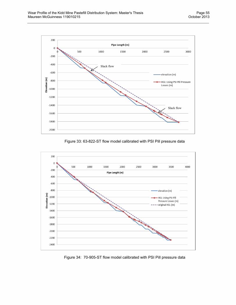
Wear Profile of the Kidd Mine Pastefill Distribution System: Master's Thesis Page 55 Maureen McGuinness 119010215 October 2013
Figure 33: 63-822-ST flow model calibrated with PSI Pill pressure data
Figure 34: 70-905-ST flow model calibrated with PSI Pill pressure data
Slack flow
Slack flow

Wear Profile of the Kidd Mine Pastefill Distribution System: Master's Thesis Page 56 Maureen McGuinness 119010215 October 2013
Figure 35: 66-GW1-ST flow model calibrated with PSI Pill pressure data
Figure 36: 66-745-ST flow model calibrated with PSI Pill pressure data
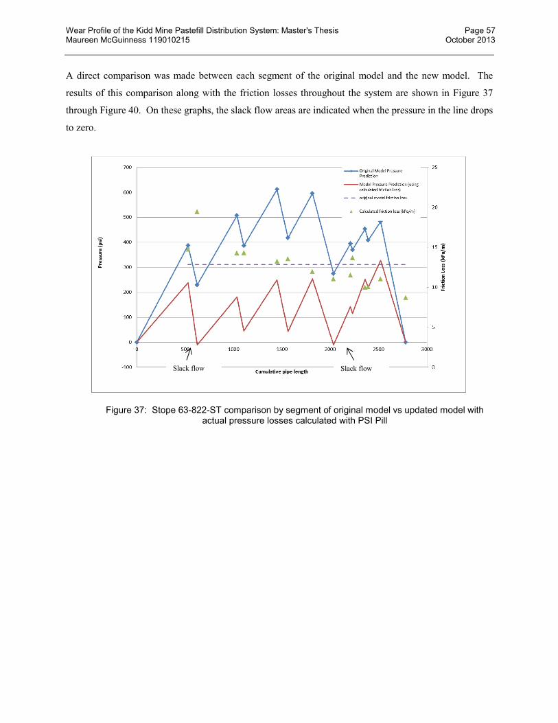
Wear Profile of the Kidd Mine Pastefill Distribution System: Master's Thesis Page 57 Maureen McGuinness 119010215 October 2013
A direct comparison was made between each segment of the original model and the new model. The
results of this comparison along with the friction losses throughout the system are shown in Figure 37
through Figure 40. On these graphs, the slack flow areas are indicated when the pressure in the line drops
to zero.
Figure 37: Stope 63-822-ST comparison by segment of original model vs updated model with actual pressure losses calculated with PSI Pill
Slack flow Slack flow
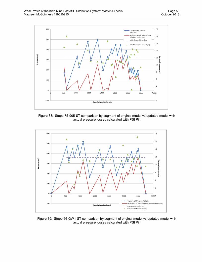
Wear Profile of the Kidd Mine Pastefill Distribution System: Master's Thesis Page 58 Maureen McGuinness 119010215 October 2013
Figure 38: Stope 75-905-ST comparison by segment of original model vs updated model with actual pressure losses calculated with PSI Pill
Figure 39: Stope 66-GW1-ST comparison by segment of original model vs updated model with actual pressure losses calculated with PSI Pill

Wear Profile of the Kidd Mine Pastefill Distribution System: Master's Thesis Page 59 Maureen McGuinness 119010215 October 2013
Figure 40: Stope 65-745-ST comparison by segment of original model vs updated model with actual pressure losses calculated with PSI Pill
5.8 Flow Analysis
5.8.1 Friction
The average friction loss in the system was examined over time, as expressed in terms of throughput.
Figure 41 shows that the friction losses dropped by 1 kPa/m during the first million tonnes of production
and have remained stable, at around 11.8 kPa/m, for the next 1.5 million tonnes of paste produced. Apart
from test 2, the average PSI Pill results are in agreement with the pressure loss used in the original model.
This result seems at odds with the differences between the two models shown in Section 5.7 which
showed different friction readings to the original model.

Wear Profile of the Kidd Mine Pastefill Distribution System: Master's Thesis Page 60 Maureen McGuinness 119010215 October 2013
Figure 41: Friction losses vs time as measured in terms of system throughput
The next step was to look at the pressure loss in the different sections of the system.
There is a fairly good correspondence between the two models at the start of the system, as shown in
Figure 37 through Figure 40, however, after 4600 level, the models diverge – only coming together again
at the bottom level. Since these trends were even seen in the first two years of operation (63-822-ST and
75-905-ST) it seems unlikely they were caused by changes in internal pipe diameter, due to wear. The
loops on all levels were made of the same pipe material and had the same original diameter. This
indicates that another factor was causing the change in friction loss conditions, such as the paste material
itself or piping configuration. The main cause for this divergence seems to be that the friction in the line
is changing as the material travels through the system.
All the friction data was combined and normalised by cumulative distance travelled. In general, there
seems to be a loss of friction over distance in the first 2500 meters of the system, as seen in Figure 42.
After the 2500 meter mark, the friction losses become more randomised or stabilise. A higher friction loss
at the start causes the pressures on the levels to drop lower than predicted by the original model. This
causes the first loops on the upper levels to approach zero pressure as the material enters the top of the
next borehole – a slack flow condition.
The data from the four tests are isolated and presented in Figure 43.
Test #1
Test #2
Test #3
Test #4
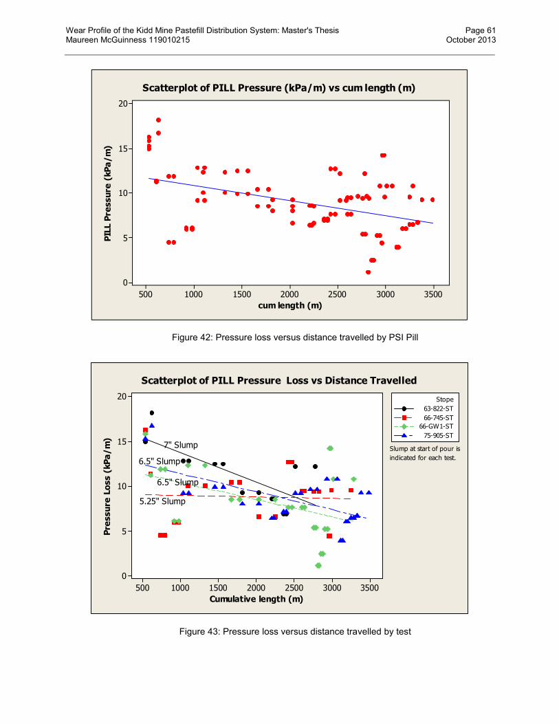
Wear Profile of the Kidd Mine Pastefill Distribution System: Master's Thesis Page 61 Maureen McGuinness 119010215 October 2013
Figure 42: Pressure loss versus distance travelled by PSI Pill
Figure 43: Pressure loss versus distance travelled by test
350030002500200015001000500
20
15
10
5
0
cum length (m)
PIL
L P
ressu
re (
kP
a/
m)
Scatterplot of PILL Pressure (kPa/m) vs cum length (m)
350030002500200015001000500
20
15
10
5
0
Cumulative length (m)
Pre
ssu
re L
oss (
kP
a/
m)
63-822-ST
66-745-ST
66-GW1-ST
75-905-ST
Stope
7" Slump
6.5" Slump
6.5" Slump
5.25" Slump
Scatterplot of PILL Pressure Loss vs Distance Travelled
indicated for each test.
Slump at start of pour is

Wear Profile of the Kidd Mine Pastefill Distribution System: Master's Thesis Page 62 Maureen McGuinness 119010215 October 2013
While the data is scattered, there seems to be a relationship between the regressions of the slopes of the
pressure loss versus distance travelled for three of the stopes, while the fourth stope pour’s regression is
almost flat. By comparing the regressions with the starting paste slump, it can be seen that the regression
line for the two pours at the same starting slump are parallel. The pour at the higher slump (thinner
consistency) has a steeper slope and the low slump pour (thicker paste) has the flat regression trend.
This analysis suggests that the pressure losses change as the pastefill travels through the system and are
affected by the initial paste consistency. This is different than the regular approach to modelling the
system hydraulics where a constant pressure loss is assumed for the whole system
5.8.2 Paste Interface in the Boreholes
The tops of boreholes for sections between surface-1600 level, 2800-3800 level and 46K-5200 boreholes
seem particularly susceptible to free fall, as shown by their dips below zero pressure. The accelerometer
readings also spike in these areas, indicating free fall or slack flow. The 63-822-ST and the 66-745-ST
stope pours show difficulty with the first borehole. In these pours, the ultimate pressure in the surface to
1600 borehole of the 66-745-ST is very low (140 psi) indicating that the borehole is not full. This
suggests that the top of that borehole would be under vacuum with free fall of paste until it reached the
paste interface further down the boreholes. In fact, in all the tests, the pressure profiles indicate that the
surface to 1600 level borehole was not full. Using the energy balance with friction losses calculated from
the PSI Pill data the paste height in the borehole can be estimated, as shown in Table IX.
Table IX: Calculated height of paste interface in the surface – 1600 borehole
63-822-ST 75-905-ST 66-GW1-ST 66-745-ST
Pressure on 1600 (psi) (kPa)
260 1792.4
240 1654.5
420 2895.5
140 965.2
Friction loss (kPa/m) 12.05 9.90 10.03 9.95
Height of paste interface (m) 236.7 170.2 301.8 99.8
% of borehole 45% 32% 58% 19%
5.8.3 Velocity
In the original flow model, the velocity was calculated by the volume of paste passing through an internal
pipe cross sectional area. Thus, the velocities only varied in accordance with the inside diameter of the
pipes in the system, giving three distinct velocities. The PSI Pill data allowed the direct measurement of
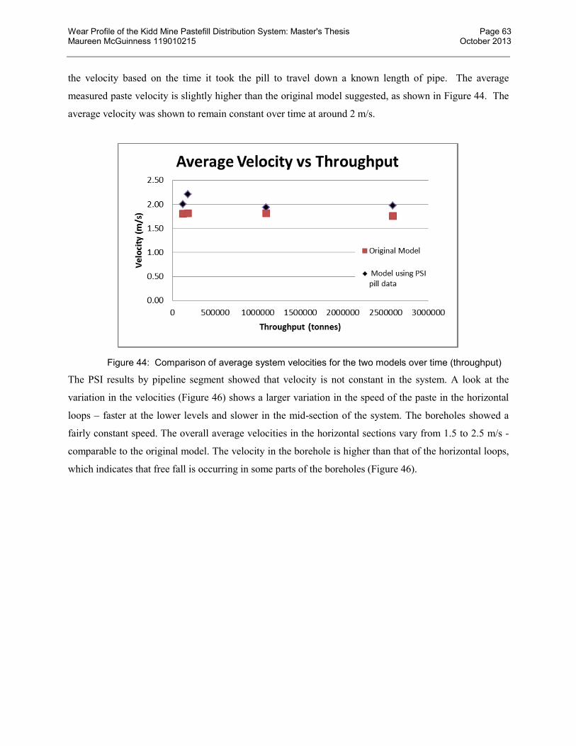
Wear Profile of the Kidd Mine Pastefill Distribution System: Master's Thesis Page 63 Maureen McGuinness 119010215 October 2013
the velocity based on the time it took the pill to travel down a known length of pipe. The average
measured paste velocity is slightly higher than the original model suggested, as shown in Figure 44. The
average velocity was shown to remain constant over time at around 2 m/s.
Figure 44: Comparison of average system velocities for the two models over time (throughput)
The PSI results by pipeline segment showed that velocity is not constant in the system. A look at the
variation in the velocities (Figure 46) shows a larger variation in the speed of the paste in the horizontal
loops – faster at the lower levels and slower in the mid-section of the system. The boreholes showed a
fairly constant speed. The overall average velocities in the horizontal sections vary from 1.5 to 2.5 m/s -
comparable to the original model. The velocity in the borehole is higher than that of the horizontal loops,
which indicates that free fall is occurring in some parts of the boreholes (Figure 46).

Wear Profile of the Kidd Mine Pastefill Distribution System: Master's Thesis Page 64 Maureen McGuinness 119010215 October 2013
Figure 45: Velocity range in the horizontal loops - divided by location in the system
Figure 46: Velocity range in the boreholes - divided by location in the system
5.8.4 Temperature
While temperature is not usually considered a significant factor in slurry wear, it is related to wear in that
it is a by-product of the wear and friction process. It can also impact the corrosion rate which in turn can
amplify the pipe wear. By the end of the paste’s travel to the stope, all the potential energy in the paste
due to gravity is transformed to pressure energy and then dissipated to friction and ultimately dissipates as
heat. Therefore, heat gain can be an indicator of wear. Heat gain may also be associated with the ambient
0
5
10
15
20
25
30
0 0.5 1 1.5 2 2.5 3 3.5 4
Velocity Mid (5200-6800lvl)
Lower (6900 - 7500lvl) Upper (surf-4600lvl)

Wear Profile of the Kidd Mine Pastefill Distribution System: Master's Thesis Page 65 Maureen McGuinness 119010215 October 2013
temperature of the rock and the drifts which generally increase with depth at the Kidd Mine and also with
the exothermic reaction associated with cement hydration.
The PSI Pill measures the temperature of the paste as it travels to the open stope. Analysis of the PSI Pill
temperature readings is limited by the thermocouple resolution. The temperature is measured to the
nearest degree, resulting in step increments in temperature. The data shows that temperature increases
with distance of the piping run (Figure 47) at the rate of approximately 0.004 °C/m.
Figure 47: Temperature gain vs distance travelled
The four tests showed an initial increase in temperature followed by a plateau and then an increase again.
The plateau occurs between the 3800 level 5600 level section. This reduction in heat gain may be due to
an extended time in horizontal run where ventilation may offset temperature gains.
The individual PSI Pill tests are differentiated on the graph in Figure 48. One difference in the
temperature gain is the starting point. Two tests showed a large increase in temperature in the first
borehole whereas the other tests indicated a loss in temperature. This is possibly an effect of ambient
temperature at the start of the test. The two tests which showed an initial drop in temperature were taken
during the spring/summer. The pill may have been warmed by handling and so had an initial negative
temperature adjustment as it was introduced into the paste. The other two tests were done in winter so that
350030002500200015001000500
17.5
15.0
12.5
10.0
7.5
5.0
2.5
0.0
Total length
To
tal Te
mp
Ga
in (
C)
Scatterplot of Total Temp Gain (C) vs Total length
R-Sq = 74.7%
Total Temp Gain (C) = - 1.41 + 0.00433 Total length

Wear Profile of the Kidd Mine Pastefill Distribution System: Master's Thesis Page 66 Maureen McGuinness 119010215 October 2013
the instruments may have been cooler and actually warmed up as they were introduced to the paste. In
winter, hot water is added to the paste to keep the paste temperature constant.
Figure 48: Temperature gain vs distance travelled - by stope
The fact that corrosion can be accelerated with temperature may explain why the relationship of wear rate
vs piping distance could not be concluded statistically. If corrosion is increasing at depth, it may be
offsetting the decrease in wear due to particle degradation.
350030002500200015001000500
17.5
15.0
12.5
10.0
7.5
5.0
2.5
0.0
Total length
To
tal Te
mp
Ga
in (
C)
63-822-ST
66-745-ST
66-GW1-ST
75-905-ST
Stope
Scatterplot of Total Temp Gain (C) vs Total length

Wear Profile of the Kidd Mine Pastefill Distribution System: Master's Thesis Page 67 Maureen McGuinness 119010215 October 2013
5.9 Summary
The goal of this stage was to develop the flow model from first principles for the Kidd Mine distribution
system and calibrate it with in-situ pressure readings from the PSI Pill data. This exercise revealed some
of the distribution system flow characteristics.
Pressure
Pressures balance among levels as seen by substantial pressure reduction during the progression
along the horizontal loops.
Some pipe segments are in vacuum/free fall. This is indicated in flow models and supported by
PSI Pill results.
Friction Losses
Fairly constant friction losses develop in the system over the operation life – average 12 kPa/m
Overall friction factor, as used in the original hydraulic model, was in line with the average
friction factor measured by the PSI Pill.
Friction does change throughout the system, in general dropping as the paste progresses through
the pipeline, particularly during the first 2500 m of travel.
Applying the friction factors based on measurement, rather than applying an overall friction
factor, provides a more accurate picture of the flow of paste through the system.
Velocity
Fairly constant velocity occurs in the system over the operation life – average 2 m/s
Variation in loop velocities are seen when individual pipe segment velocities are examined.
Temperature
Constant temperature gain occurs with pipeline length of 0.003 °C/m
Temperature gain is mostly produced in the boreholes, whose lengths are more significant.

Wear Profile of the Kidd Mine Pastefill Distribution System: Master's Thesis Page 68 Maureen McGuinness 119010215 October 2013
6. PASTE CHARACTERISATION
The properties of the materials used to make the paste and those of the paste itself are examined in the
following sections.
6.1 Tailings Particle Size Distribution
The particle size distribution of the tailings is determined through screening and blending of the the
excavated tailings at the tailings area. The specification for the final tailings product is as follows:
Before 2010: 40-60% passing 20μm
After 2010: 45-65% passing 20μm
The change in range in 2010 allowed for more tailings recovery from the site. The paste recipe
(sand:tailings ratio and binder content) will be adjusted for the increased fines content, as needed, to meet
the pastefill strength and transport requirements.
The size distribution in Figure 49 shows that this sample, taken in 2012, was within the specification of
tailings between 45% and 65% -20 μm (actual value 55%). The specific gravity of the tailings was
determined to be 2.74 based on the average of three tests.
Figure 49: Particle size distribution of 2012 sample of tailings, sand, final paste product and a calculated particle size of final paste product (combined at 50:50 ratio) with no binder included
Specification for tailings
45-65% passing 20 μm
(as of 2010)
Specification for paste
20% passing 20 μm
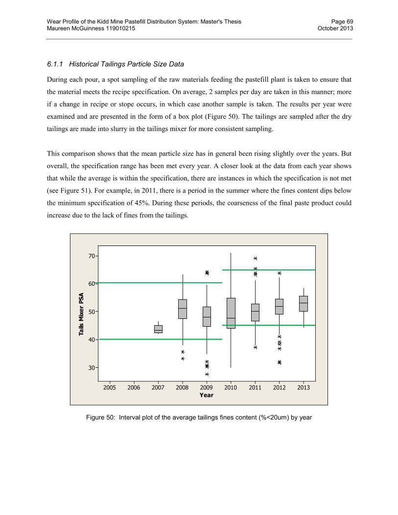
Wear Profile of the Kidd Mine Pastefill Distribution System: Master's Thesis Page 69 Maureen McGuinness 119010215 October 2013
6.1.1 Historical Tailings Particle Size Data
During each pour, a spot sampling of the raw materials feeding the pastefill plant is taken to ensure that
the material meets the recipe specification. On average, 2 samples per day are taken in this manner; more
if a change in recipe or stope occurs, in which case another sample is taken. The results per year were
examined and are presented in the form of a box plot (Figure 50). The tailings are sampled after the dry
tailings are made into slurry in the tailings mixer for more consistent sampling.
This comparison shows that the mean particle size has in general been rising slightly over the years. But
overall, the specification range has been met every year. A closer look at the data from each year shows
that while the average is within the specification, there are instances in which the specification is not met
(see Figure 51). For example, in 2011, there is a period in the summer where the fines content dips below
the minimum specification of 45%. During these periods, the coarseness of the final paste product could
increase due to the lack of fines from the tailings.
Figure 50: Interval plot of the average tailings fines content (%<20um) by year
201320122011201020092008200720062005
70
60
50
40
30
Year
Ta
ils M
ixe
r P
SA

Wear Profile of the Kidd Mine Pastefill Distribution System: Master's Thesis Page 70 Maureen McGuinness 119010215 October 2013
Figure 51: 2011 Tailings particle size results over time
6.2 Sand Fineness Modulus
The specification for the sand a fineness modulus (FM) between 2.1 and 2.9. The Fineness Modulus for
the sand sample in Figure 49 is 2.75. Fineness Modulus is a parameter used in the concrete industry to
standardize the gradation of concrete mixes to provide a prediction of paste consistency. A constant FM
between samples indicates that approximately the same amount of water is present and that the
workability of the samples should be similar (Bittencourt, Fontoura et al. 2001). Samples can be graded to
have the same FM without having the same percent of material in each size fraction. The formula used at
the Kidd Mine pastefill plant to calculate the sand FM is as follows:
20-N
ov-11
20-S
ep-1
1
19-A
ug-11
22-Jul-1
1
31-M
ay-11
29-A
pr-1
1
25-M
ar-11
01-M
ar-1
1
30-Jan
-11
01-Jan
-11
70
65
60
55
50
45
40
Date
Ta
ils M
ixe
r P
SA
(%
<2
0u
m)
Time Series Plot of 2011 Tails Mixer PSA
�� = � %���� ��������
�
�� �
where:
n= standard set of seven sieves
(10mm, 5mm,2.5mm,1.25mm, 0.630mm, 0.315mm and 0.160mm)
Equation 6-1
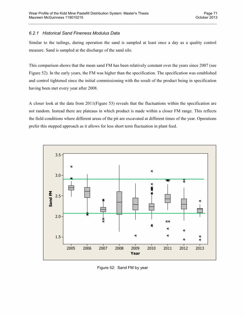
Wear Profile of the Kidd Mine Pastefill Distribution System: Master's Thesis Page 71 Maureen McGuinness 119010215 October 2013
6.2.1 Historical Sand Fineness Modulus Data
Similar to the tailings, during operation the sand is sampled at least once a day as a quality control
measure. Sand is sampled at the discharge of the sand silo.
This comparison shows that the mean sand FM has been relatively constant over the years since 2007 (see
Figure 52). In the early years, the FM was higher than the specification. The specification was established
and control tightened since the initial commissioning with the result of the product being in specification
having been met every year after 2008.
A closer look at the data from 2011(Figure 53) reveals that the fluctuations within the specification are
not random. Instead there are plateaus in which product is made within a closer FM range. This reflects
the field conditions where different areas of the pit are excavated at different times of the year. Operations
prefer this stepped approach as it allows for less short term fluctuation in plant feed.
Figure 52: Sand FM by year
201320122011201020092008200720062005
3.5
3.0
2.5
2.0
1.5
Year
Sa
nd
FM

Wear Profile of the Kidd Mine Pastefill Distribution System: Master's Thesis Page 72 Maureen McGuinness 119010215 October 2013
Figure 53: 2011 Sand FM results over time
6.3 Chemical Analysis and Mineralogy
The sand and McIntyre tailings were analysed by the Kidd Mine for mineralogy and chemical content and
provided for this study. The mineralogical distributions are found in Table X and Table XI. The Mohs
hardness values for each mineral are also provided. The sand is high in quartz, albite and orthoclase, with
these three minerals representing 80% of the sand composition. The tailings have a similar composition
with quartz, albite and dolomite representing over 80% of the tailings composition.
Table X: Esker sand mineralogy7
7 Semi-Quantitative Analysis by Rietveld Method (Phase in wt%): results provided by the Kidd Mine 8 taken from Mindat.org
20-N
ov-11
20-S
ep-1
1
19-A
ug-11
22-Jul-1
1
31-M
ay-1
1
29-A
pr-11
25-M
ar-1
1
01-M
ar-11
30-Jan
-11
01-Jan
-11
3.00
2.75
2.50
2.25
2.00
1.75
1.50
Date
Sa
nd
FM
Time Series Plot of 2011 Sand FM
Mineral Formula wt% Mohs hardness8
Quartz SiO2 37.38 7
Albite NaAlSi3O8 29.31 6-6.5
Orthoclase KAlSi3O8 13.28 6-6.5
Calcite CaCO3 6.95 3

Wear Profile of the Kidd Mine Pastefill Distribution System: Master's Thesis Page 73 Maureen McGuinness 119010215 October 2013
Table XI: McIntyre tailings mineralogy9
The minerals were sorted by relative hardness and the hardness of steel pipe added, as seen in Table XII.
A large portion of the sand and the tailings mineral components (80% and 60% respectively) have a
greater Mohs hardness than steel, implying that these minerals can degrade a steel surface. While the
Mohs scale is only relative and can’t be used quantitatively to arrive at a weighted average hardness
value, the abundance of hard minerals in the sand and tailings make up does indicate that their properties
will have an influence on the behavior of the minerals, in terms of wear.
Due to the fact that both the sand and the gold mine tailings had a high quantity of quartz and albite, a
Kidd Creek tailings mineralogy published in 1995 (Blowes, Lortie et al. 1995) was also added to the
comparison to see if there were any significant mineralogical differences in the Cu-Zn tailings produced
at the Kidd concentrator and the gold tailings used in the Kidd paste.
This comparison is surprising because there was operational experience that suggested that the tailings
were more abrasive than the sand; the loader blade teeth were changed out twice as often at the tailings
9 Semi-Quantitative Analysis by Rietveld Method (Phase in wt%): results provided by Kidd Mine
Chlorite (MgAl)6(Si,Al)4O10(OH)8 4.60 2-2.5
Actinolite Ca2(Mg,Fe+2)5SiO8O22(OH)2 4.15 5-6
Dolomite CaMg(CO3)2 2.50 3.5-4
Muscovite KAl2Si3Al10(OH)2 1.83 2-2.5
Mineral Formula wt% Mohs hardness
Quartz SiO2 33.81 7
Albite NaAlSi3O8 27.10 6-6.5
Dolomite Ca(Mg,Fe)(CO3)2 20.80 3.5-4
Chlorite (MgAl)6(Si,Al)4O10(OH)8 9.82 2-2.5
Calcite CaCO3 2.86 3
Gypsum CaSO4 2.71 1.5-2
Muscovite (K,Na)(Al,Mg,Fe)2(Si3.1Al0.9)O10(OH) 1.81 2-2.5
Pyrite FeS2 1.09 6-6.5
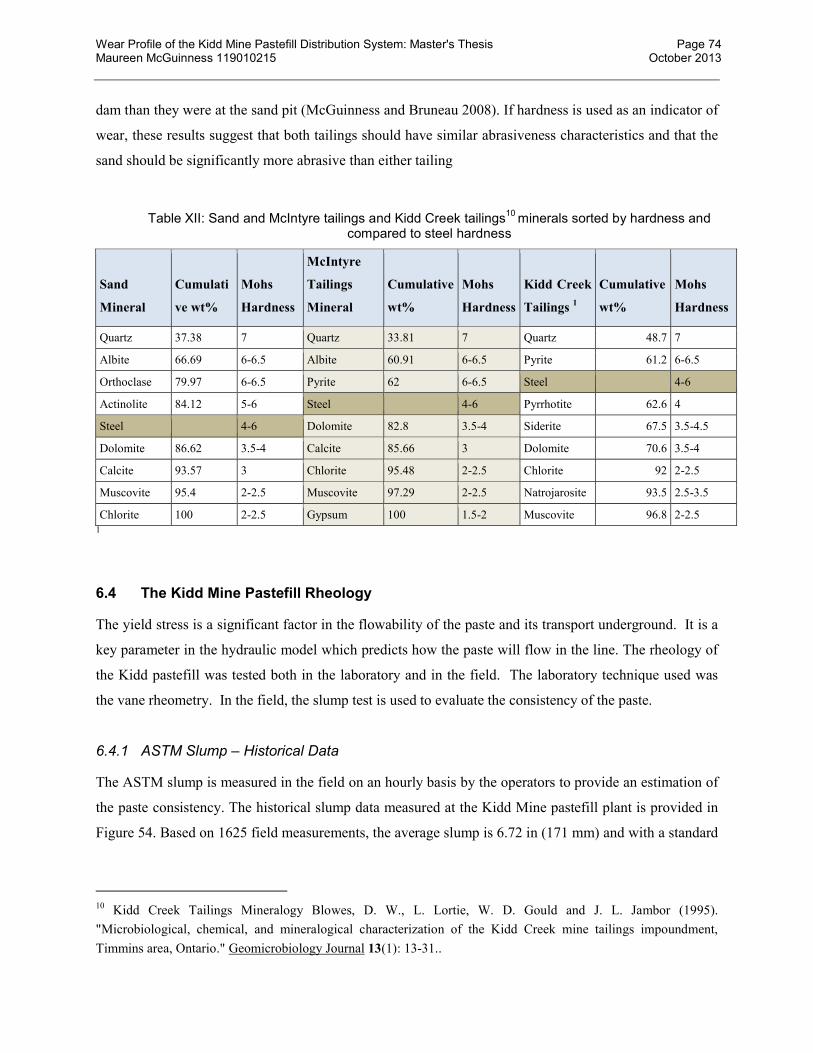
Wear Profile of the Kidd Mine Pastefill Distribution System: Master's Thesis Page 74 Maureen McGuinness 119010215 October 2013
dam than they were at the sand pit (McGuinness and Bruneau 2008). If hardness is used as an indicator of
wear, these results suggest that both tailings should have similar abrasiveness characteristics and that the
sand should be significantly more abrasive than either tailing
Table XII: Sand and McIntyre tailings and Kidd Creek tailings10
minerals sorted by hardness and compared to steel hardness
Sand
Mineral
Cumulati
ve wt%
Mohs
Hardness
McIntyre
Tailings
Mineral
Cumulative
wt%
Mohs
Hardness
Kidd Creek
Tailings 1
Cumulative
wt%
Mohs
Hardness
Quartz 37.38 7 Quartz 33.81 7 Quartz 48.7 7
Albite 66.69 6-6.5 Albite 60.91 6-6.5 Pyrite 61.2 6-6.5
Orthoclase 79.97 6-6.5 Pyrite 62 6-6.5 Steel 4-6
Actinolite 84.12 5-6 Steel 4-6 Pyrrhotite 62.6 4
Steel 4-6 Dolomite 82.8 3.5-4 Siderite 67.5 3.5-4.5
Dolomite 86.62 3.5-4 Calcite 85.66 3 Dolomite 70.6 3.5-4
Calcite 93.57 3 Chlorite 95.48 2-2.5 Chlorite 92 2-2.5
Muscovite 95.4 2-2.5 Muscovite 97.29 2-2.5 Natrojarosite 93.5 2.5-3.5
Chlorite 100 2-2.5 Gypsum 100 1.5-2 Muscovite 96.8 2-2.5 1
6.4 The Kidd Mine Pastefill Rheology
The yield stress is a significant factor in the flowability of the paste and its transport underground. It is a
key parameter in the hydraulic model which predicts how the paste will flow in the line. The rheology of
the Kidd pastefill was tested both in the laboratory and in the field. The laboratory technique used was
the vane rheometry. In the field, the slump test is used to evaluate the consistency of the paste.
6.4.1 ASTM Slump – Historical Data
The ASTM slump is measured in the field on an hourly basis by the operators to provide an estimation of
the paste consistency. The historical slump data measured at the Kidd Mine pastefill plant is provided in
Figure 54. Based on 1625 field measurements, the average slump is 6.72 in (171 mm) and with a standard
10 Kidd Creek Tailings Mineralogy Blowes, D. W., L. Lortie, W. D. Gould and J. L. Jambor (1995).
"Microbiological, chemical, and mineralogical characterization of the Kidd Creek mine tailings impoundment,
Timmins area, Ontario." Geomicrobiology Journal 13(1): 13-31..

Wear Profile of the Kidd Mine Pastefill Distribution System: Master's Thesis Page 75 Maureen McGuinness 119010215 October 2013
deviation of 0.64 in. Half of the data from 2005 to 2012 were within the range of 6.25 and 7.25 in (159 to
184 mm).
Figure 54: Historical slump data 2005-2012
The breakdown of the slump data by year (Figure 55) shows that the average slump dropped to its lowest
point in 2007 which aligns with the highest wear rates measured in the piping system (refer to Figure 17).
This was a reaction to the system running in slack flow – reducing the slump (thickening up the paste)
added more friction in the system and helped back the pastefill up into the boreholes.
The average slump increased in later years, which corresponds to the installation of the restrictions
underground and new ceramic lined boreholes which increased the friction in the pipeline.
8.58.07.57.06.56.05.55.0
Median
Mean
6.756.746.736.726.716.706.69
1st Q uartile 6.2500
Median 6.7500
3rd Q uartile 7.2500
Maximum 8.5000
6.6867 6.7487
6.7500 6.7500
0.6165 0.6604
A -Squared 11.57
P-V alue < 0.005
Mean 6.7177
StDev 0.6376
V ariance 0.4066
Skewness -0.005298
Kurtosis -0.248908
N 1625
Minimum 5.0000
A nderson-Darling Normality Test
95% C onfidence Interv al for Mean
95% C onfidence Interv al for Median
95% C onfidence Interv al for StDev95% Confidence Intervals

Wear Profile of the Kidd Mine Pastefill Distribution System: Master's Thesis Page 76 Maureen McGuinness 119010215 October 2013
Figure 55: Historical slump data for the Kidd pastefill plant by year
6.4.2 ASTM Slump – Laboratory Testing
In the laboratory, the relationship between slump and % solids was tested. From the slump curve in
Figure 56, it is seen that the common range of slumps for the Kidd Mine paste (6.25 to 7.25in)
corresponds to a % solids range of 81.6 and 82.2 %. Percent solids can be used to relate the slump to the
yield stress.
There is not a direct relationship between ASTM slump and the yield stress. It is used as an indicator of
the consistency of the paste, of which yield stress is not the sole factor. However, a similar test has been
developed that can be directly related to yield stress: the Boger slump test (Pashias, Boger et al. 1996).
This test was not used in this evaluation because it was not historically measured at the Kidd Mine
pastefill plant. In the future, this could be a way to collect data that can be incorporated directly into the
pastefill hydraulic model.
201320122011201020092008200720062005
9
8
7
6
5
AS
TM
Slu
mp
(in
)

Wear Profile of the Kidd Mine Pastefill Distribution System: Master's Thesis Page 77 Maureen McGuinness 119010215 October 2013
Figure 56: ASTM Slump measurements vs % solids for the Kidd paste;with and without binder (data provided by Kidd Mine)
6.4.3 Vane Rheometry
The vane viscometer provides the static yield stress of the paste. The results of the vane rheometry
testing were provided by the Kidd Mine and are shown in Figure 57. For the % solids range established in
Section 6.4.2, the yield stress of the Kidd Mine paste (containing binder) ranges from 355 to 550 Pa.
The abundance of large particles (>150μm) in the Kidd Mine pastefill prohibits the use of concentric
rheometry, which has a very close gap between the spindle and the cup wall. Therefore, the values for
dynamic yield stress and paste viscosity that are derived from this type of test are not available.
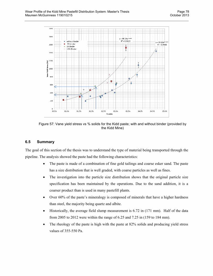
Wear Profile of the Kidd Mine Pastefill Distribution System: Master's Thesis Page 78 Maureen McGuinness 119010215 October 2013
Figure 57: Vane yield stress vs % solids for the Kidd paste; with and without binder (provided by the Kidd Mine)
6.5 Summary
The goal of this section of the thesis was to understand the type of material being transported through the
pipeline. The analysis showed the paste had the following characteristics:
The paste is made of a combination of fine gold tailings and coarse esker sand. The paste
has a size distribution that is well graded, with coarse particles as well as fines.
The investigation into the particle size distribution shows that the original particle size
specification has been maintained by the operations. Due to the sand addition, it is a
coarser product than is used in many pastefill plants.
Over 60% of the paste’s mineralogy is composed of minerals that have a higher hardness
than steel, the majority being quartz and albite.
Historically, the average field slump measurement is 6.72 in (171 mm). Half of the data
from 2005 to 2012 were within the range of 6.25 and 7.25 in (159 to 184 mm).
The rheology of the paste is high with the paste at 82% solids and producing yield stress
values of 355-550 Pa.
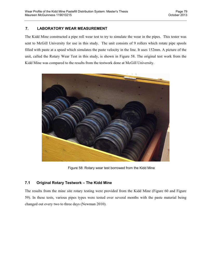
Wear Profile of the Kidd Mine Pastefill Distribution System: Master's Thesis Page 79 Maureen McGuinness 119010215 October 2013
7. LABORATORY WEAR MEASUREMENT
The Kidd Mine constructed a pipe roll wear test to try to simulate the wear in the pipes. This tester was
sent to McGill University for use in this study. The unit consists of 9 rollers which rotate pipe spools
filled with paste at a speed which simulates the paste velocity in the line. It uses 152mm. A picture of the
unit, called the Rotary Wear Test in this study, is shown in Figure 58. The original test work from the
Kidd Mine was compared to the results from the testwork done at McGill University.
Figure 58: Rotary wear test borrowed from the Kidd Mine
7.1 Original Rotary Testwork – The Kidd Mine
The results from the mine site rotary testing were provided from the Kidd Mine (Figure 60 and Figure
59). In these tests, various pipes types were tested over several months with the paste material being
changed out every two to three days (Newman 2010).

Wear Profile of the Kidd Mine Pastefill Distribution System: Master's Thesis Page 80 Maureen McGuinness 119010215 October 2013
Figure 59: Original rotary test results by the Kidd Mine – mass loss vs time (Newman 2010)
Figure 60: The Kidd Mine rotary wear test results – thickness loss per 100 kt paste throughput (Newman 2010)
The tests did not well replicate the actual wear rates measured in the field. The average in-situ results are
twice the wear rate of the X52 #2 results. The general trend of wear for different pipe types was as
expected. The steel pipes exhibited more wear than the overlay pipes and the ceramic pipes showed less
wear.

Wear Profile of the Kidd Mine Pastefill Distribution System: Master's Thesis Page 81 Maureen McGuinness 119010215 October 2013
It is suspected that the X52#1 pipe sample was improperly named as the wear rates do not fit the trend
produced by the rest of the wear tests, though this could not be confirmed either way. From this initial test
work, it was seen that the rotary test results were fairly linear. This fact raises the potential for the number
of cycles per test to be reduced for future tests. This would save time and conserve paste sample material.
7.2 Wear Test Development at McGill University
Pipe spools for the test were provided by the Kidd Mine. They are made from API 5L X52 pipe used in
the Kidd Mine pastefill distribution system. In the original tests that were performed at the mine, the
spools were 381 mm long. The ends of the spools were closed off using PVC pipe caps. Paste was placed
in the spool sections and the sealed spool was placed on the rotary table for a defined period of time. The
weight of the spool before and after the test was measured. This wear rate was related to the number of
rotations of the spool which replicates passage of paste through the pipeline.
To increase the accuracy of the weighing process, the spools were reduced in length for the McGill
University tests. The spools were cut into 127 mm long spools. The ends of each spool were closed off
using shortened pipe caps which leaked due to the lack of a gasket. This resulted in the loss of water from
the sample and caused the samples to form balls in the spools instead of remaining a paste, as shown in
Figure 61. A new spool cap was designed and successfully implemented by the McGill undergraduate and
post-doctorate working on the project. This new cap is shown in Figure 62 and Figure 63.
Figure 61: Leaking end caps and the resulting balls of paste caused by loss of water
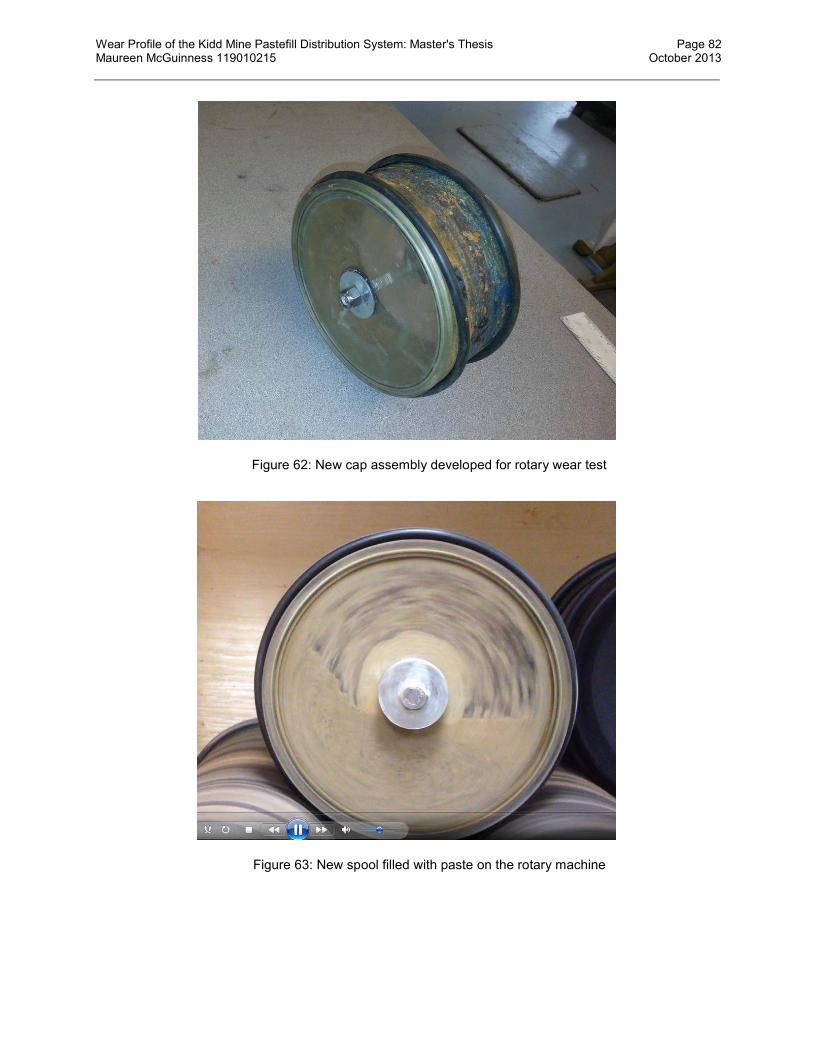
Wear Profile of the Kidd Mine Pastefill Distribution System: Master's Thesis Page 82 Maureen McGuinness 119010215 October 2013
Figure 62: New cap assembly developed for rotary wear test
Figure 63: New spool filled with paste on the rotary machine

Wear Profile of the Kidd Mine Pastefill Distribution System: Master's Thesis Page 83 Maureen McGuinness 119010215 October 2013
7.2.1 Particle Degradation
Because the paste particles will degrade over time as they roll around in the pipe spool, part of the rotary
test procedure is to change-out the paste material in the spool regularly. This attempts to replicate the
actual pipe environment in which the paste material contacting the wall is constantly being refreshed as
the paste flows by. Other wear tests have shown the effect of degradation of the wear material during the
test. For example, in the Toroidal test- a test with some similarities to the rotary test - a degradation curve
was established for the material. It was shown that the wear rate decreased exponentially with increasing
time before material replacement (Cooke, Johnson et al. 2000). They proposed a procedure to relate the
lab wear results with degradation back to a wear rate equivalent with fresh material.
To evaluate the extent of degradation during the rotary test, the particle size distribution of samples left in
the rotary test for 0,1,2,3 and 7 days was measured. Samples of the tailings after each of these timed
intervals were sent for particle shape and particle size analysis.
Particle shape analysis was performed by the University of Alberta Department of Chemical and
Materials Engineering - Pipeline Transport Processes Research Group using a FPIA (SYSMEX/Malvern
Flow Particle Image Analyzer). This instrument takes pictures of each particle and assigns a circularity
value according to how closely the particle resembles a circle. Data from all particles measured is
combined in histogram form as shown in Figure 64. A slurry undergoing degradation will have an
increase in the frequency of circle-like particles as the angular points are abraded off during transport.
This effect was seen in the rotary degradation test. There is a shift to the right of the histogram for the 7
day results when compared to the original sample shape characteristics (Day 0) and the frequency of
particles with circularity around 0.9 increased slightly.

Wear Profile of the Kidd Mine Pastefill Distribution System: Master's Thesis Page 84 Maureen McGuinness 119010215 October 2013
Figure 64: Circularity of the tailings samples 7 days in the rotary tester overlapped with day 0 results (measured using FPIA)
Particle size analysis was performed by Paterson & Cooke using a Malvern Particle Size Analyser. The
shift in particle size after 3 and 7 days in the rotary test is shown in Figure 65. There is considerable
change after 7 days while the 3 day sample still exhibits a similar size curve to the original specimen.
By comparing the change in percent passing (Figure 66), is it shown that the amount of material passing
the 10 μm size fraction increases with increasing time in the rotary test. By day 7 there is a 4% increase in
material finer than 15 μm. The results at day 1 to day 3 show the degradation progression. The results at
day 1 show an accumulation of 15 μm particles (decrease in % passing) created as the 100 μm particles
wore down (increase in % passing). By day 2, the +100 μm particles were ground down to the 100 μm
size (a decrease in % passing at this level). The new 100 μm fraction was ground down further by day 3
(an increase in % passing at the 100 μm and the 50 μm sizes)
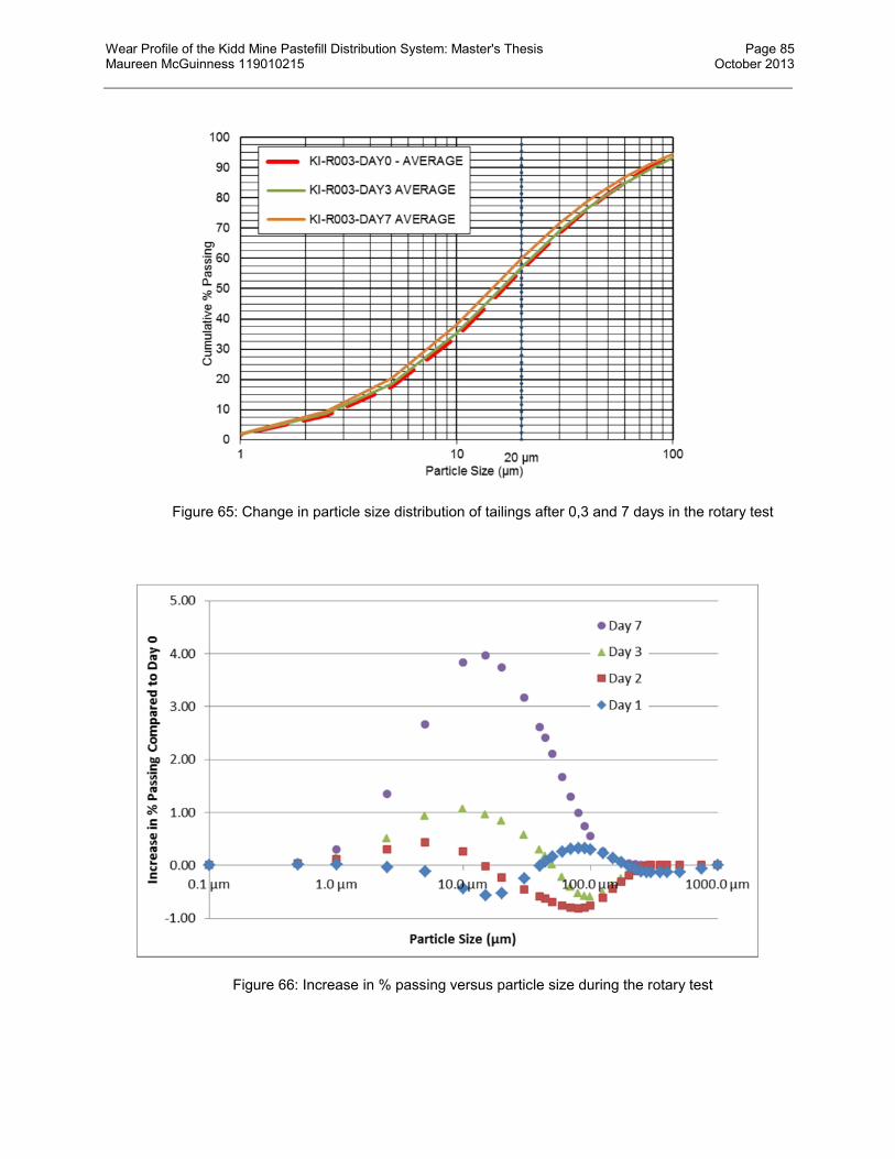
Wear Profile of the Kidd Mine Pastefill Distribution System: Master's Thesis Page 85 Maureen McGuinness 119010215 October 2013
Figure 65: Change in particle size distribution of tailings after 0,3 and 7 days in the rotary test
Figure 66: Increase in % passing versus particle size during the rotary test

Wear Profile of the Kidd Mine Pastefill Distribution System: Master's Thesis Page 86 Maureen McGuinness 119010215 October 2013
This degradation test indicates that, after two days, there is particle degradation but the production of
minus 15 μm material is limited to 1% during this period. Taking these results into consideration, for the
rotary test procedure, it was chosen to switch out the material every two to three days to minimize the
effect of degradation on the wear rates measured in the tests.
7.2.2 Rotary Wear Test Procedure
Samples of tailings and sand, binder and water were provided by the Kidd Mine for the laboratory test
work. The characteristics of this material were discussed in Section 6. This material was blended
following the pastefill recipe used at the Kidd Mine. For the laboratory wear tests, it was not possible to
add binder in the recipe as it would cause the paste to set. The rotary testing was performed on un-
cemented blends only. The recipe used was a blend of sand and tailings at a 50/50 dry ratio with solids
concentration of 80%. An example of the recipe is provided in Appendix D. Three replicate tests were
performed for each test condition. Three wear rates are calculated individually and then averaged for the
final test result.
One cycle of the rotary wear test consists of two to three changes of paste after which the mass loss of the
spool is calculated. A breakdown of a rotary test cycle is shown in Table XIII.
Table XIII: Rotary test cycle
Step Action Data Collected
1 Weigh and measure the empty, dry spool (end caps
removed)
Initial dry spool mass, in g
Initial spool ID, in mm
Pipe spool width, in mm
Pipe density, in g/cm3
2 Prepare paste recipe to test. Paste % solids, recipe
3 Assemble the end caps and add the paste to the spool.
4 Place on rotary table for 2 days. Rotary tester rpm
Time on wear tester
5 Replace the material in the spool with fresh paste and
return to rotary table for 2 days.
Rotary tester rpm
Time on wear tester

Wear Profile of the Kidd Mine Pastefill Distribution System: Master's Thesis Page 87 Maureen McGuinness 119010215 October 2013
6 Replace the material in the spool with fresh paste and
return to rotary table for 2 days.
Rotary tester rpm
Time on wear tester
7 Empty and dry the spool
8 Weigh the empty, dry spool (end caps removed) Final dry spool mass, in g
After each cycle, the new inside diameter is calculated from the mass loss, using Equation 7-1. This is
converted into pipe thickness loss (Equation 7-2). The velocity of the paste in the pipe is calculated, as
shown in Equation 7-3, using the rpm of the rotary table and the surface area of the pipe that is in contact
with the paste (based on visual inspection, 1/3 of the circumference is in contact with the paste at any one
time, refer to Figure 63). From the data collected, the loss of pipe thickness is calculated for an equivalent
paste throughput.
One disadvantage of this calculation of wear rate is that it is correlated to the full tonnage of paste flowing
through the cross sectional area of the pipe even though only very little of this overall tonnage actually
comes in contact with the pipe wall. This could mask the wear results because there may be a point after
which the wear rate is not further influenced by the increasing concentration or tonnage. In those cases
the wear rate would be underestimated by the wear test.
���� = ������ +
�������
���
�
�������
�
where:
Dnew = New spool ID at end of the cycle, m
Vlost= Volume of pipe material removed, m3
Lspool = Length of the spool, m
Do = Original Spool ID, m
Equation 7-1
�����=
���� − ��
2
where:
tlost = pipe thickness lost, m
Equation 7-2
� ����� =���
3������× ��� (60���)× �
where:
Mequiv = Equivalent paste throughput, t/h
rpm = Rotary table rotations per minute
ρ = Paste density, t/m3
Equation 7-3
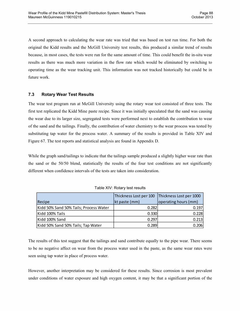
Wear Profile of the Kidd Mine Pastefill Distribution System: Master's Thesis Page 88 Maureen McGuinness 119010215 October 2013
A second approach to calculating the wear rate was tried that was based on test run time. For both the
original the Kidd results and the McGill University test results, this produced a similar trend of results
because, in most cases, the tests were run for the same amount of time. This could benefit the in-situ wear
results as there was much more variation in the flow rate which would be eliminated by switching to
operating time as the wear tracking unit. This information was not tracked historically but could be in
future work.
7.3 Rotary Wear Test Results
The wear test program run at McGill University using the rotary wear test consisted of three tests. The
first test replicated the Kidd Mine paste recipe. Since it was initially speculated that the sand was causing
the wear due to its larger size, segregated tests were performed next to establish the contribution to wear
of the sand and the tailings. Finally, the contribution of water chemistry to the wear process was tested by
substituting tap water for the process water. A summary of the results is provided in Table XIV and
Figure 67. The test reports and statistical analysis are found in Appendix D.
While the graph sand/tailings to indicate that the tailings sample produced a slightly higher wear rate than
the sand or the 50/50 blend, statistically the results of the four test conditions are not significantly
different when confidence intervals of the tests are taken into consideration.
Table XIV: Rotary test results
The results of this test suggest that the tailings and sand contribute equally to the pipe wear. There seems
to be no negative affect on wear from the process water used in the paste, as the same wear rates were
seen using tap water in place of process water.
However, another interpretation may be considered for these results. Since corrosion is most prevalent
under conditions of water exposure and high oxygen content, it may be that a significant portion of the
Recipe
Thickness Lost per 100
kt paste (mm)
Thickness Lost per 1000
operating hours (mm)
Kidd 50% Sand 50% Tails; Process Water 0.282 0.197
Kidd 100% Tails 0.330 0.228
Kidd 100% Sand 0.297 0.213
Kidd 50% Sand 50% Tails; Tap Water 0.289 0.206
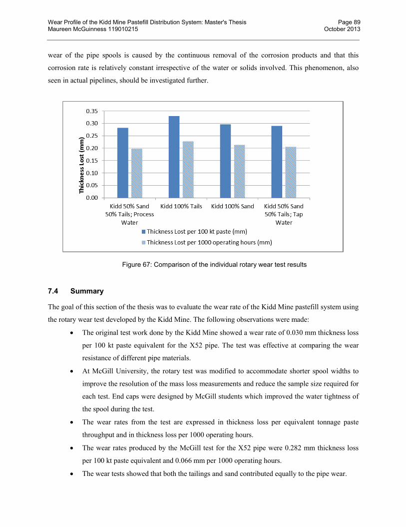
Wear Profile of the Kidd Mine Pastefill Distribution System: Master's Thesis Page 89 Maureen McGuinness 119010215 October 2013
wear of the pipe spools is caused by the continuous removal of the corrosion products and that this
corrosion rate is relatively constant irrespective of the water or solids involved. This phenomenon, also
seen in actual pipelines, should be investigated further.
Figure 67: Comparison of the individual rotary wear test results
7.4 Summary
The goal of this section of the thesis was to evaluate the wear rate of the Kidd Mine pastefill system using
the rotary wear test developed by the Kidd Mine. The following observations were made:
The original test work done by the Kidd Mine showed a wear rate of 0.030 mm thickness loss
per 100 kt paste equivalent for the X52 pipe. The test was effective at comparing the wear
resistance of different pipe materials.
At McGill University, the rotary test was modified to accommodate shorter spool widths to
improve the resolution of the mass loss measurements and reduce the sample size required for
each test. End caps were designed by McGill students which improved the water tightness of
the spool during the test.
The wear rates from the test are expressed in thickness loss per equivalent tonnage paste
throughput and in thickness loss per 1000 operating hours.
The wear rates produced by the McGill test for the X52 pipe were 0.282 mm thickness loss
per 100 kt paste equivalent and 0.066 mm per 1000 operating hours.
The wear tests showed that both the tailings and sand contributed equally to the pipe wear.

Wear Profile of the Kidd Mine Pastefill Distribution System: Master's Thesis Page 90 Maureen McGuinness 119010215 October 2013
The wear tests showed that the Kidd Mine process water did not contribute significantly to the
wear rates.
Corrosion may contribute significantly to the wear results in this test and should be
investigated further.
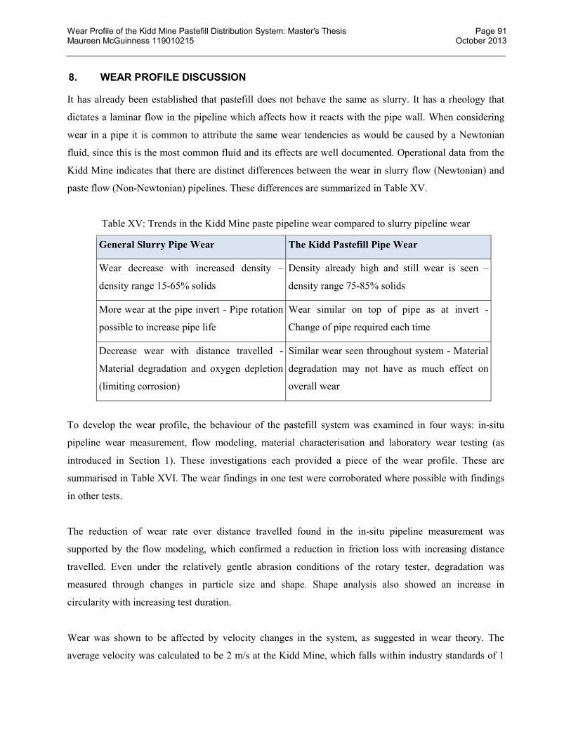
Wear Profile of the Kidd Mine Pastefill Distribution System: Master's Thesis Page 91 Maureen McGuinness 119010215 October 2013
8. WEAR PROFILE DISCUSSION
It has already been established that pastefill does not behave the same as slurry. It has a rheology that
dictates a laminar flow in the pipeline which affects how it reacts with the pipe wall. When considering
wear in a pipe it is common to attribute the same wear tendencies as would be caused by a Newtonian
fluid, since this is the most common fluid and its effects are well documented. Operational data from the
Kidd Mine indicates that there are distinct differences between the wear in slurry flow (Newtonian) and
paste flow (Non-Newtonian) pipelines. These differences are summarized in Table XV.
Table XV: Trends in the Kidd Mine paste pipeline wear compared to slurry pipeline wear
General Slurry Pipe Wear The Kidd Pastefill Pipe Wear
Wear decrease with increased density –
density range 15-65% solids
Density already high and still wear is seen –
density range 75-85% solids
More wear at the pipe invert - Pipe rotation
possible to increase pipe life
Wear similar on top of pipe as at invert -
Change of pipe required each time
Decrease wear with distance travelled -
Material degradation and oxygen depletion
(limiting corrosion)
Similar wear seen throughout system - Material
degradation may not have as much effect on
overall wear
To develop the wear profile, the behaviour of the pastefill system was examined in four ways: in-situ
pipeline wear measurement, flow modeling, material characterisation and laboratory wear testing (as
introduced in Section 1). These investigations each provided a piece of the wear profile. These are
summarised in Table XVI. The wear findings in one test were corroborated where possible with findings
in other tests.
The reduction of wear rate over distance travelled found in the in-situ pipeline measurement was
supported by the flow modeling, which confirmed a reduction in friction loss with increasing distance
travelled. Even under the relatively gentle abrasion conditions of the rotary tester, degradation was
measured through changes in particle size and shape. Shape analysis also showed an increase in
circularity with increasing test duration.
Wear was shown to be affected by velocity changes in the system, as suggested in wear theory. The
average velocity was calculated to be 2 m/s at the Kidd Mine, which falls within industry standards of 1

Wear Profile of the Kidd Mine Pastefill Distribution System: Master's Thesis Page 92 Maureen McGuinness 119010215 October 2013
to 2 m/s but is on the high end. Looking at the range of velocities throughout the system, it was seen that
the velocities range from 1 to 4 m/s, particularly in the boreholes indicating the presence of slack flow
areas. This was confirmed by the hydraulic analysis which showed that several of the boreholes were
susceptible to slack flow (for example, the surface to 1600 level borehole was shown to be only around
50% full). The in-situ data also related increases in velocity to increases in wear. Higher wear rates were
measured in 2007 when more of the system was in slack flow, to which high velocities are associated.
Table XVI: The Kidd Mine wear profile components
Source Wear Profile
In-situ pipeline wear measurement
• Wear constant along horizontal loops • Constant or decreasing wear with travel distance • Constant wear over system life • The mean wear rate of 0.60 mm/100kt of paste throughput
Flow modeling of pipeline system
• Constant friction loss over system life of 11.8 kPa/m • Decrease in friction loss vs distance travelled (up to 2500m) • Velocity average 2 m/s - slightly higher in boreholes than on horizontal runs
Material Characterisation
• Paste particle size = 22% -20�m • 60% of minerals in paste are harder than steel • High yield stress (355 to 550 Pa)
Laboratory Testing
• Tailings and sand contribute equally to wear • Process water does not contribute to wear when compared to tap water • Corrosion is suspected to play an important role in the wear. • Average rotary test wear rate for 50/50 paste recipe = 0.289 mm/100kt of
equivalent paste throughput
In wear theory, shape and size of the particles are considered influential to the wear rate. The fines
content of the Kidd Mine paste is at the borderline of what is considered acceptable for reliable paste flow
in the line (22% vs 15% recommended minimum). This is due to the large portion of sand supplementing
the tailings in the paste. Operations that use only full plant tailings have a fines content of 40 to 60%. The
larger particles of the sand component contribute to the high wear rates.
However, both the hardness evaluation and the laboratory wear testing suggested that the tailings and the
sand contribute to wear and to a relatively similar degree. Over 60% of the mineral composition of both
the tailings and the sand is harder than steel making steel susceptible to wear from both components. This
conclusion is collaborated by the rotary test which produced little difference in wear rates between tests
done with 100% sand and those with 100% tailings. The 50/50 recipe also gave similar wear results.

Wear Profile of the Kidd Mine Pastefill Distribution System: Master's Thesis Page 93 Maureen McGuinness 119010215 October 2013
8.1 Summary
The wear profile of the Kidd Mine pastefill distribution system can be summarised as follows:
The Kidd Mine pastefill distribution system wear profile is characterised by erosion - corrosion wear
which is relatively uniform throughout the system and over time, with an average wear rate of 0.6 mm /
100 kt paste throughput. There are indications of decreasing wear rate with increasing distance of paste
travel. Contributing to this wear are the tailings and sand component of the paste which both contain over
60% of material harder than the steel of which the pipeline system is made. The paste consists of 22%
fines which is just over the minimum amount of fines recommended for paste flow. The paste has a high
yield stress (355 to 550 Pa) and friction losses of 11.8 kPa/m. The system exhibits full pressurised,
laminar flow which results in uniform wear distribution around the circumference of the pipe except in
slack flow areas, in which case the wear is dominantly at the pipe invert. Velocities in the system average
2 m/s but can increase to 4 m/s in some areas, particularly in the boreholes. The pipeline configuration is
such that increasing diameter of pipe due to wear make the boreholes susceptible to slack flow which in
turn further accelerates the wear in these areas.
Wear Profile of the Kidd Mine Pastefill Distribution System: Master's Thesis Page 94 Maureen McGuinness 119010215 October 2013
9. FUTURE WORK
This thesis was a first attempt at defining a wear profile for a pastefill system. As each pastefill system
has its own unique wear system, this approach could be applied to other pastefill systems with the goal of
finding a methodology that could indicate the wear profile of pastefill systems and especially of proposed
systems so that wear can be incorporated into the system design, operation and maintenance plans.
The following outlines some specific areas of future work arising from this research that are
recommended.
In-situ Wear Testing
Wear measurements around the pipe circumference to see difference of invert to top of pipe to
confirm laminar flow
Better definition of flow distance versus wear rate relationship
Better control of wear measurement for less variation in field data – fewer sites but better
controlled
Perform more recent PSI Pill test to evaluate the effect of the borehole and piping changes done
to increase friction in the line
Investigate the effect of start-up and shut-down on wear.
Hydraulic Modeling
Investigate ways to incorporate changes in friction in the model without the input of the PSI Pill
test
Validate the PSI Pill calibration process with in-situ pressure gauges and an external pressure
source before running the test.
Paste Characterisation
Evaluate the use of Boger slump tests versus ASTM slump measurement for more rheological
information
Shape analysis of the in-situ worn and fresh particles for comparison with wear information
Incorporate the yield stress and plastic viscosity parameters found in rheology testing into the
hydraulic model and link to % solids and estimate of slump for the pour.
Laboratory Wear Testing
More testing using the rotary wear test procedure to confirm if tailings wear rate is significantly
higher than that of sand
Incorporate a way to evaluate the influence of corrosion on the rotary wear test results

Wear Profile of the Kidd Mine Pastefill Distribution System: Master's Thesis Page 95 Maureen McGuinness 119010215 October 2013
Investigate / develop other wear testers that would replicate wear in a paste system better than the
rotary wear test.
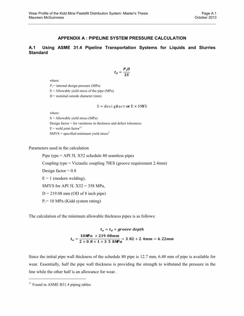
Wear Profile of the Kidd Mine Pastefill Distribution System: Master's Thesis Page A.1 Maureen McGuinness October 2013
APPENDIX A : PIPELINE SYSTEM PRESSURE CALCULATION
A.1 Using ASME 31.4 Pipeline Transportation Systems for Liquids and Slurries Standard
Parameters used in the calculation
Pipe type = API 5L X52 schedule 80 seamless pipes
Coupling type = Victaulic coupling 70ES (groove requirement 2.4mm)
Design factor = 0.8
E = 1 (modern welding),
SMYS for API 5L X52 = 358 MPa,
D = 219.08 mm (OD of 8 inch pipe)
Pi = 10 MPa (Kidd system rating)
The calculation of the minimum allowable thickness pipes is as follows:
Since the initial pipe wall thickness of the schedule 80 pipe is 12.7 mm, 6.48 mm of pipe is available for
wear. Essentially, half the pipe wall thickness is providing the strength to withstand the pressure in the
line while the other half is an allowance for wear.
11 Found in ASME B31.4 piping tables
�� =���
��
where:
Pi = internal design pressure (MPa)
S = Allowable yield stress of the pipe (MPa)
D = nominal outside diameter (mm)
S = designfactor× E × SMYS
where:
S = Allowable yield stress (MPa)
Design factor = for variations in thickness and defect tolerances
E = weld joint factor11
SMYS = specified minimum yield stress3
�� = �� + �����������
�� =����� × ���.����
� × �.� × � × ������= �.�� + �.��� = �.����
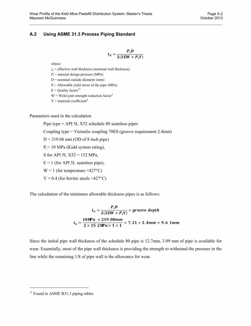
Wear Profile of the Kidd Mine Pastefill Distribution System: Master's Thesis Page A.2 Maureen McGuinness October 2013
A.2 Using ASME 31.3 Process Piping Standard
Parameters used in the calculation
Pipe type = API 5L X52 schedule 80 seamless pipes
Coupling type = Victaulic coupling 70ES (groove requirement 2.4mm)
D = 219.08 mm (OD of 8 inch pipe)
Pi = 10 MPa (Kidd system rating),
S for API 5L X52 = 152 MPa,
E = 1 (for API 5L seamless pipe),
W = 1 (for temperature <427°C)
Y = 0.4 (for ferritic steels <427°C)
The calculation of the minimum allowable thickness pipes is as follows:
Since the initial pipe wall thickness of the schedule 80 pipe is 12.7mm, 3.09 mm of pipe is available for
wear. Essentially, most of the pipe wall thickness is providing the strength to withstand the pressure in the
line while the remaining 1/8 of pipe wall is the allowance for wear.
12 Found in ASME B31.3 piping tables
�� =���
�(��� + ���)
where:
td = effective wall thickness (nominal wall thickness)
Pi = internal design pressure (MPa)
D = nominal outside diameter (mm)
S = Allowable yield stress of the pipe (MPa)
E = Quality factor12
W = Weld joint strength reduction factor4
Y = material coefficient4
�� =
���
�(��� + ���)+ �����������
�� =����� × ���.����
� × ������× � × �= �.�� + �.��� = �.����

Wear Profile of the Kidd Mine Pastefill Distribution System: Master's Thesis Page B.1 Maureen McGuinness October 2013
APPENDIX B : PSI PILL TEST LOGS
B.1 63-822-ST PSI Pill Test January 13, 2005
Operator Log during the PSI Pill Test Slump Data during the PSI Pill Test
13-Jan-05Batcher Dave
Stope 63-822-st
mix-main4
8:00 mike on 6000-ok
9:00 guy called from 5600-ok
9:20 pete on 2800-ok
9:30 sand system plugged
10:20 w/a flush
10:31 w/a flush
10:38 water flush
10:39 slick
10:48 slump 7 ¾ temp 27
10:56 slump 7 temp 24.3
11:10 pressure loss on 38A and 46, stopped batch
11:39 start again
12:00 slump 6, temp 16.4
12:08 slump 6 ¼ temp 16.4
12:09 1600 pete said ok
12:20 slump 6 ½ temp 16.2
12:38 slump 7, sent with pill
12:44 slump 7 ¾ temp 17
12:54 slump 6 ¼ temp 15
12:40 stop tailing feed
1:00 batch last load
1:10 w/a flush
1:26 w/a flush
1:33 w/a flush
Time to stope: 24 min
Slump
-28 min 6.25
-18 min 6.5
With pill 7
+6 min 7.75
+16 min 6.25

Wear Profile of the Kidd Mine Pastefill Distribution System: Master's Thesis Page B.2 Maureen McGuinness October 2013
B.2 75-905-ST PSI Pill Test February 13, 2005
Operator Log during the PSI Pill Test Slump Data during the PSI Pill Test
Febuary 13 2005
Batrcher Dave
Stope 75-905-ST
Mix main4
7:45 sand hang ups in bin ,feed too slow to continue,call shutdown
7:58 w/a flush
8:12 w/a flush
8;25 w/a flush
10:05 delay cancelled ,start again
10:08 w/a flush
10:19 water and slick
10:44 slump 6 ¼ temp 8.2
11:02 stuff received on 7400
11;26 slump 6 ¾ temp 12.5
12:22 sent ball
12:30 slump 6 ¾ temp 11.7
1:15 pill on its way
1;33 slump 6 ½ temp 12.3
2:10 received pill
2;25 cap1
2;42 slump 6 ½ temp11.2
3:12 slump 6 ¾ temp 13.1
3;59 slump 6 ½ temp 13
5:02 last batch
5:12 w/a flush
5:36 w/a flush
5:48 w/a flush
Slump
-45min 6.75
sent pill 6.5 estimate
+18min 6.5
+77 min 6.5
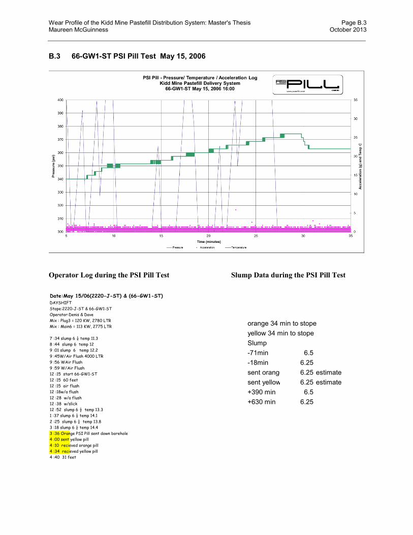
Wear Profile of the Kidd Mine Pastefill Distribution System: Master's Thesis Page B.3 Maureen McGuinness October 2013
B.3 66-GW1-ST PSI Pill Test May 15, 2006
Operator Log during the PSI Pill Test Slump Data during the PSI Pill Test
Date:May 15/06(2220-J-ST) & (66-GW1-ST)
DAYSHIFT
Stope:2220-J-ST & 66-GW1-ST
Operator:Denis & Dave
Mix : Plug3 = 120 KW, 2780 LTR
Mix : Main6 = 113 KW, 2775 LTR
7 :34 slump 6 ¼ temp 11.3
8 :44 slump 6 temp 12
9 :01 slump 6 temp 12.2
9 :45W/Air Flush 4000 LTR
9 :56 WAir Flush
9 :59 W/Air Flush
12 :15 start 66-GW1-ST
12 :15 60 feet
12 :15 air flush
12 :18w/a flush
12 :28 w/a flush
12 :38 w/slick
12 :52 slump 6 ½ temp 13.3
1 :37 slump 6 ½ temp 14.1
2 :25 slump 6 ½ temp 13.8
3 :18 slump 6 ¼ temp 14.4
3 :36 Orange PSI Pill sent down borehole
4 :00 sent yellow pill
4 :10 recieved orange pill
4 :34 recieved yellow pill
4 :40 31 feet
orange 34 min to stope
yellow 34 min to stope
Slump
-71min 6.5
-18min 6.25
sent orange 6.25 estimate
sent yellow 6.25 estimate
+390 min 6.5
+630 min 6.25
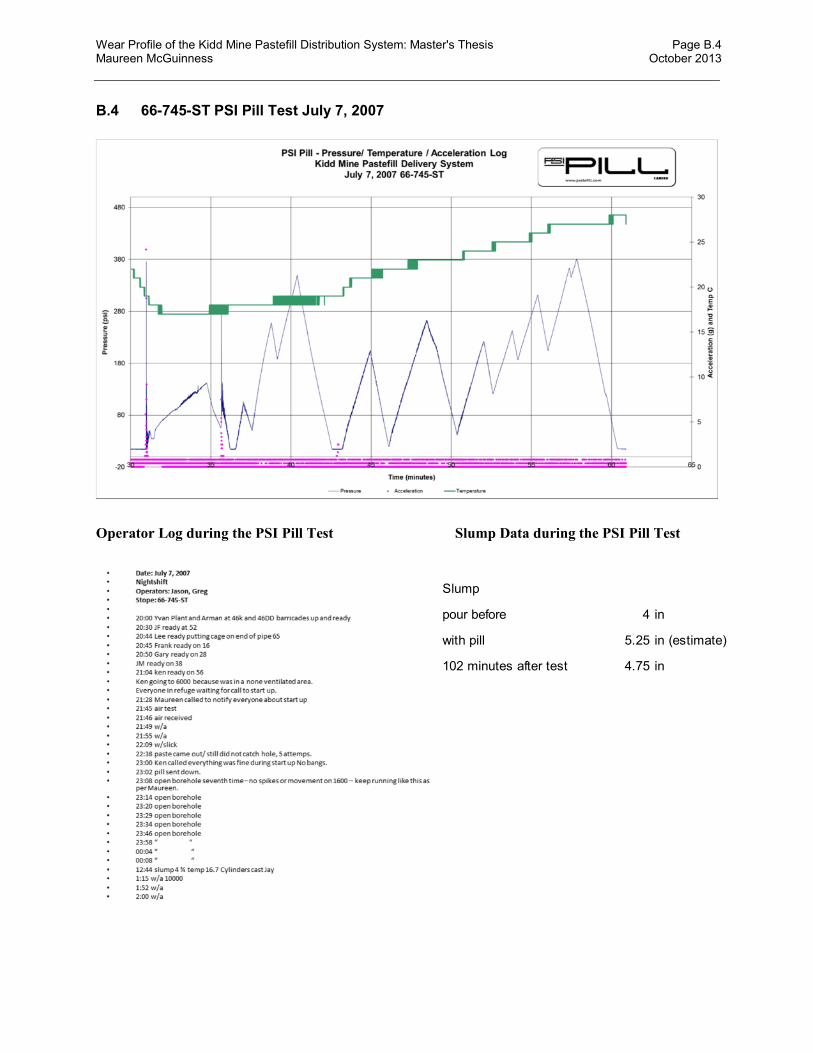
Wear Profile of the Kidd Mine Pastefill Distribution System: Master's Thesis Page B.4 Maureen McGuinness October 2013
B.4 66-745-ST PSI Pill Test July 7, 2007
Operator Log during the PSI Pill Test Slump Data during the PSI Pill Test
Slump
pour before 4 in
with pill 5.25 in (estimate)
102 minutes after test 4.75 in
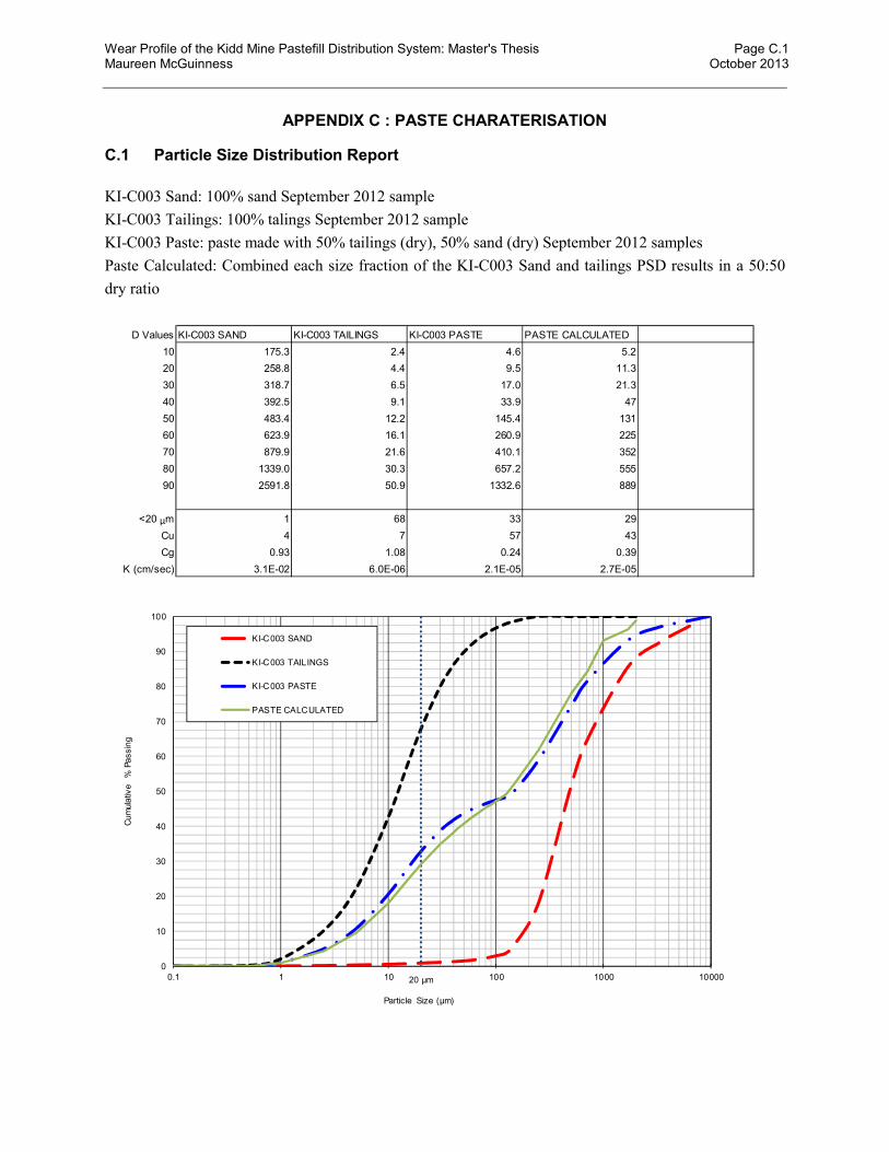
Wear Profile of the Kidd Mine Pastefill Distribution System: Master's Thesis Page C.1 Maureen McGuinness October 2013
APPENDIX C : PASTE CHARATERISATION
C.1 Particle Size Distribution Report
KI-C003 Sand: 100% sand September 2012 sample
KI-C003 Tailings: 100% talings September 2012 sample
KI-C003 Paste: paste made with 50% tailings (dry), 50% sand (dry) September 2012 samples
Paste Calculated: Combined each size fraction of the KI-C003 Sand and tailings PSD results in a 50:50
dry ratio
D Values KI-C003 SAND KI-C003 TAILINGS KI-C003 PASTE PASTE CALCULATED
10 175.3 2.4 4.6 5.2
20 258.8 4.4 9.5 11.3
30 318.7 6.5 17.0 21.3
40 392.5 9.1 33.9 47
50 483.4 12.2 145.4 131
60 623.9 16.1 260.9 225
70 879.9 21.6 410.1 352
80 1339.0 30.3 657.2 555
90 2591.8 50.9 1332.6 889
<20 µm 1 68 33 29
Cu 4 7 57 43
Cg 0.93 1.08 0.24 0.39
K (cm/sec) 3.1E-02 6.0E-06 2.1E-05 2.7E-05
20 µm
0
10
20
30
40
50
60
70
80
90
100
0.1 1 10 100 1000 10000
Cum
ula
tive
% P
assin
g
Particle Size (µm)
KI-C003 SAND
KI-C003 TAILINGS
KI-C003 PASTE
PASTE CALCULATED
Wear Profile of the Kidd Mine Pastefill Distribution System: Master's Thesis Page C.2 Maureen McGuinness October 2013
Procedure: The sample was dried and weighed before being wet screened at 150 μm. Size analysis on the
minus 150μm material was performed using a particle size analyzer. The plus 150μm material was dry
screened. The results were combined. This is a procedure that is used in many industrial labs, including
Paterson & Cooke. The methods differ significantly; the dry screening measures weight and can be
influenced by particle shape while the PSA measures by volume and the results can be influenced by
variation in particle density. Strictly speaking, it is not advisable to mix the two methods but each of the
individual methods has drawbacks that make them undesirable to use solely on their own. Larger particles
tend to settle out of solution during the PSA measurements while screening at 400 mesh (37 μm) and 600
mesh (25 μm) only provides two points of information in an important section of the particle size curve.
Due to these constraints, it was decided to use this joint method for the screening of the paste material
components.
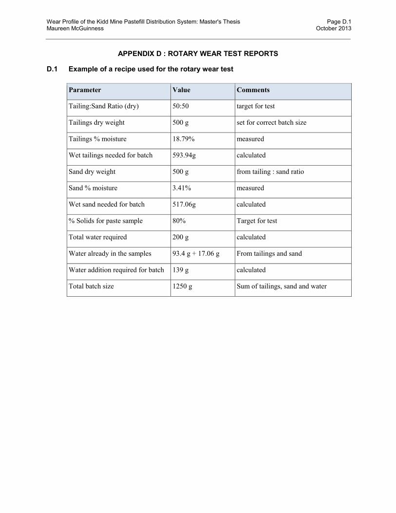
Wear Profile of the Kidd Mine Pastefill Distribution System: Master's Thesis Page D.1 Maureen McGuinness October 2013
APPENDIX D : ROTARY WEAR TEST REPORTS
D.1 Example of a recipe used for the rotary wear test
Parameter Value Comments
Tailing:Sand Ratio (dry) 50:50 target for test
Tailings dry weight 500 g set for correct batch size
Tailings % moisture 18.79% measured
Wet tailings needed for batch 593.94g calculated
Sand dry weight 500 g from tailing : sand ratio
Sand % moisture 3.41% measured
Wet sand needed for batch 517.06g calculated
% Solids for paste sample 80% Target for test
Total water required 200 g calculated
Water already in the samples 93.4 g + 17.06 g From tailings and sand
Water addition required for batch 139 g calculated
Total batch size 1250 g Sum of tailings, sand and water

Wear Profile of the Kidd Mine Pastefill Distribution System: Master's Thesis Page D.2 Maureen McGuinness October 2013
D.2 Paste Recipe Investigation: Kidd Mine 50% Tails and 50% Sand; Process Water
KI-R004 Kidd 50% Sand 50% Tails; Process Water
Spool Type X52 #1
Recipe Kidd 50% Sand 50% Tails; Process Water
Density 7.77
Spool length 0.062615
CycleSpool RPM
Test Time (hrs)
Cumulative Test Time
(hours)
Incremental Mass Loss
(g)
Cumulative Mass Loss
(g)
Volume lost
(m3)
Spool ID (m)
Incremental Thickness
Lost
(mm)
Cumulative Thickness
Lost
(mm)
Spool Area in contact with
paste
(m2)
Paste Velocity (m/s)
Flow Rate of Paste
(tonnes/hour)
Equivalent throughput of paste in pipe
(tonnes)
Cumulative
Thickness Lost per 100000 tonnes(mm/100000
tonnes)
Measured Pipe
ID
(m)
Start 37 0.0 0 0.0 0.0 0 0.155750 0.0000 0.0000 0.0102 0.3017 23.296 0 0.0000
Cycle 1 37 162.5 163 2.3 2.3 2.960E-07 0.155769 0.0097 0.0097 0.0102 0.3018 23.302 3787 0.2551
Cycle 2 37 160.1 323 5.5 7.8 7.079E-07 0.155816 0.0231 0.0328 0.0102 0.3019 23.316 7520 0.4356
Cycle 3 37 164.5 487 0.7 8.5 9.009E-08 0.155821 0.0029 0.0357 0.0102 0.3019 23.318 11356 0.3144
Cycle 4 37 161.9 649 2.5 11.0 3.218E-07 0.155842 0.0105 0.0462 0.0102 0.3019 23.324 15132 0.3053
Cycle 5 37 259.8 909 1.4 12.4 1.802E-07 0.155854 0.0059 0.0521 0.0102 0.3019 23.327 21192 0.2457
Volume = Mass/density thickness = (OD-ID)/2 Velocity = PI *ID*rpm
Spool Type X52 #2 Spool A in contact = PI *ID*1/3 *length
Recipe Kidd 50% Sand 50% Tails; Process Water
New ID =[ (Volume + PI *length/4*ID^2)/(PI *length/4)]^0.5 Flow Rate = Spool A * velocity*paste density
Density 7.77
Spool length 0.063585
CycleSpool RPM
Test Time (hrs)
Cumulative Test Time
(hours)
Incremental Mass Loss
(g)
Cumulative Mass Loss
(g)
Volume lost
(m3)
Spool ID (m)
Incremental Thickness
Lost(mm)
Cumulative Thickness
Lost(mm)
Spool Area in contact with
paste
(m2)
Paste Velocity (m/s)
Flow Rate of Paste
(tonnes/hour)
Equivalent throughput of paste in pipe
(tonnes)
Cumulative Thickness Lost per
100000 tonnes(mm/100000
tonnes)
Measured Pipe
ID
(m)
Start 37 0.0 0 0.0 0.0 0 0.155750 0.0000 0.0000 0.0102 0.3017 23.296 0 0.0000
Cycle 1 37 162.5 163 2.3 2.3 2.960E-07 0.155769 0.0097 0.0097 0.0102 0.3018 23.302 3787 0.2551
Cycle 2 37 160.1 323 3.8 6.1 4.891E-07 0.155801 0.0160 0.0256 0.0102 0.3018 23.312 7519 0.3407
Cycle 3 37 164.5 487 2.2 8.3 2.831E-07 0.155820 0.0092 0.0349 0.0102 0.3019 23.317 11355 0.3070
Cycle 4 37 161.9 649 2.4 10.7 3.089E-07 0.155840 0.0101 0.0449 0.0102 0.3019 23.323 15132 0.2970
Cycle 5 37 164.0 813 2.6 13.3 3.346E-07 0.155862 0.0109 0.0558 0.0102 0.3020 23.330 18958 0.2946
Spool Type X52 #3
Recipe Kidd 50% Sand 50% Tails; Process Water
Density 7.77
Spool length 0.062915
CycleSpool RPM
Test Time (hrs)
Cumulative Test Time
(hours)
Incremental Mass Loss
(g)
Cumulative Mass Loss
(g)
Volume lost
(m3)
Spool ID (m)
Incremental Thickness
Lost(mm)
Cumulative Thickness
Lost(mm)
Spool Area in contact with
paste
(m2)
Paste Velocity (m/s)
Flow Rate of Paste
(tonnes/hour)
Equivalent throughput of paste in pipe
(tonnes)
Cumulative Thickness Lost per
100000 tonnes
(mm/100000 tonnes)
Measured Pipe
ID
(m)
Start 37 0.0 0 0.0 0.0 0 0.155750 0.0000 0.0000 0.0102 0.3017 23.296 0 0.0000
Cycle 1 37 162.5 163 1.6 1.6 2.059E-07 0.155763 0.0067 0.0067 0.0102 0.3018 23.300 3786 0.1775
Cycle 2 37 160.1 323 3.9 5.5 5.019E-07 0.155796 0.0164 0.0231 0.0102 0.3018 23.310 7519 0.3072
Cycle 3 37 164.5 487 3.5 9.0 4.505E-07 0.155826 0.0147 0.0378 0.0102 0.3019 23.319 11355 0.3329
Cycle 4 37 161.9 649 1.6 10.6 2.059E-07 0.155839 0.0067 0.0445 0.0102 0.3019 23.323 15131 0.2942
Cycle 5 37 164.0 813 2.0 12.6 2.574E-07 0.155856 0.0084 0.0529 0.0102 0.3019 23.328 18958 0.2791
Test Spool Cycle
Cumulative
Test Time
(hours)
Cumulative
Thickness Lost
(mm)
Equivalent
throughput
of paste in
pipe
(tonnes)
Wear Rate
(thickness loss
per equivalent
100kt)
Wear Rate
(thickness loss
per 1000
operating
hours)
Start 0.0 0.0000 0.0
Cycle 1 162.5 0.0097 3786.6
Cycle 2 322.6 0.0328 7519.8
Cycle 3 487.1 0.0357 11355.6
Cycle 4 649.0 0.0462 15132.5
Cycle 5 908.8 0.0521 21192.1
Start 0.0 0.0000 0.0
Cycle 1 162.5 0.0097 3786.6
Cycle 2 322.6 0.0256 7519.1
Cycle 3 487.1 0.0349 11354.8
Cycle 4 649.0 0.0449 15131.6
Cycle 5 813.1 0.0558 18958.4
Start 0.0 0.0000 0.0
Cycle 1 162.5 0.0067 3786.3
Cycle 2 322.6 0.0231 7518.6
Cycle 3 487.1 0.0378 11354.6
Cycle 4 649.0 0.0445 15131.3
Cycle 5 813.1 0.0529 18957.9
0.28 0.07
0.06
0.07
0.07
X52 #1
X52 #2
X52 #3
0.25
0.30
0.30
y = 3E-06xR² = 0.9557
0.000
0.010
0.020
0.030
0.040
0.050
0.060
0.070
0.0 5000.0 10000.0 15000.0 20000.0 25000.0
Thic
kne
ss lo
st (
mm
)
Equivalent Tonnes Paste (t)
Kidd 50% Sand 50% Tails; Process WaterX52 #1X52 #2X52 #3

Wear Profile of the Kidd Mine Pastefill Distribution System: Master's Thesis Page D.3 Maureen McGuinness October 2013
D.3 Paste Recipe Investigation: Kidd 100% Tails; Process Water
KI-R004 Kidd 100% Tails; Process Water
Spool Type X52 #4
Recipe Kidd 100% Tails
Density 7.77
Spool length 0.06175
CycleSpool
RPM
Test Time
(hrs)
Cumulative
Test Time (hours)
Incremental
Mass Loss(g)
Cumulative
Mass Loss(g)
Volume lost
(m3)
Spool ID (m)
Incremental
Thickness
Lost(mm)
Cumulative
Thickness
Lost(mm)
Spool Area in contact with
paste
(m2)
Paste Velocity
(m/s)
Flow Rate of
Paste(tonnes/hour)
Throughput of
paste in pipe(tonnes)
Cumulative
Thickness Lost per
100000 tonnes(mm/100000
tonnes)
Measured Pipe
ID
(m)
Start 37 0.0 0 0.0 0.0 0 0.155750 0.0000 0.0000 0.0101 0.3017 22.974 0 0.0000
Cycle 1 37 160.1 160 1.5 1.5 1.931E-07 0.155763 0.0064 0.0064 0.0101 0.3018 22.978 3679 0.1737
Cycle 2 37 164.5 325 6.7 8.2 8.623E-07 0.155820 0.0285 0.0349 0.0101 0.3019 22.995 7462 0.4680
Cycle 3 37 161.9 487 1.2 9.4 1.544E-07 0.155830 0.0051 0.0400 0.0101 0.3019 22.998 11186 0.3579
Cycle 4 37 164.0 651 2.9 12.3 3.732E-07 0.155855 0.0123 0.0524 0.0101 0.3019 23.005 14960 0.3501
Volume = Mass/density thickness = (OD-ID)/2 Velocity = PI *ID*rpm
Spool Type X52 #5 Spool A in contact = PI *ID*1/3 *length
Recipe Kidd 100% Tails
New ID =[ (Volume + PI *length/4*ID^2)/(PI *length/4)]^0.5 Flow Rate = Spool A * velocity*paste density
Density 7.77
Spool length 0.06362
CycleSpool RPM
Test Time (hrs)
Cumulative Test Time
(hours)
Incremental Mass Loss
(g)
Cumulative Mass Loss
(g)
Volume lost
(m3)
Spool ID (m)
Incremental
Thickness Lost
(mm)
Cumulative
Thickness Lost
(mm)
Spool Area in
contact with
paste
(m2)
Paste Velocity (m/s)
Flow Rate of Paste
(tonnes/hour)
Throughput of paste in pipe
(tonnes)
Cumulative
Thickness Lost per 100000 tonnes
(mm/100000
tonnes)
Measured Pipe
ID
(m)
Start 37 0.0 0 0.0 0.0 0 0.155750 0.0000 0.0000 0.0101 0.3017 22.974 0 0.0000
Cycle 1 37 160.1 160 2.2 2.2 2.831E-07 0.155769 0.0094 0.0094 0.0101 0.3018 22.980 3679 0.2547
Cycle 2 37 164.5 325 6.5 8.7 8.366E-07 0.155824 0.0277 0.0370 0.0101 0.3019 22.996 7462 0.4965
Cycle 3 37 161.9 487 1.3 10.0 1.673E-07 0.155835 0.0055 0.0426 0.0101 0.3019 23.000 11187 0.3807
Cycle 4 37 164.0 651 1.2 11.2 1.544E-07 0.155845 0.0051 0.0477 0.0101 0.3019 23.003 14960 0.3188
Spool Type X52 #6
Recipe Kidd 100% Tails
Density 7.77
Spool length 0.06235
CycleSpool
RPM
Test Time
(hrs)
Cumulative
Test Time
(hours)
Incremental
Mass Loss
(g)
Cumulative
Mass Loss
(g)
Volume lost
(m3)
Spool ID (m)
Incremental Thickness
Lost
(mm)
Cumulative Thickness
Lost
(mm)
Spool Area in
contact with paste
(m2)
Paste Velocity
(m/s)
Flow Rate of
Paste
(tonnes/hour)
Throughput of
paste in pipe
(tonnes)
Cumulative Thickness Lost per
100000 tonnes
(mm/100000 tonnes)
Measured Pipe
ID
(m)
Start 37 0.0 0 0.0 0.0 0 0.155750 0.0000 0.0000 0.0101 0.3017 22.974 0 0.0000
Cycle 1 37 160.1 160 1.8 1.8 2.317E-07 0.155765 0.0077 0.0077 0.0101 0.3018 22.979 3679 0.2084
Cycle 2 37 164.5 325 5.3 7.1 6.821E-07 0.155810 0.0226 0.0302 0.0101 0.3019 22.992 7462 0.4052
Cycle 3 37 161.9 487 0.3 7.4 3.861E-08 0.155813 0.0013 0.0315 0.0101 0.3019 22.993 11185 0.2818
Cycle 4 37 164.0 651 2.0 9.4 2.574E-07 0.155830 0.0085 0.0400 0.0101 0.3019 22.998 14957 0.2676
Test Spool Cycle
Cumulative
Test Time
(hours)
Cumulative
Thickness
Lost
(mm)
Throughput
of paste in
pipe
(tonnes)
Wear Rate
(thickness
loss per
equivalent
100kt)
Wear Rate
(thickness loss
per 1000
operating
hours)
Start 0.0 0.0000 0.0
Cycle 1 160.1 0.0064 3679.2
Cycle 2 324.6 0.0349 7461.9
Cycle 3 486.5 0.0400 11186.0
Cycle 4 650.6 0.0524 14959.6
Start 0.0 0.0000 0.0
Cycle 1 160.1 0.0094 3679.5
Cycle 2 324.6 0.0370 7462.3
Cycle 3 486.5 0.0426 11186.7
Cycle 4 650.6 0.0477 14959.9
Start 0.0 0.0000 0.0
Cycle 1 160.1 0.0077 3679.3
Cycle 2 324.6 0.0302 7461.5
Cycle 3 486.5 0.0315 11184.9
Cycle 4 650.6 0.0400 14957.3
0.33 0.08
0.09
0.08
0.06
X52 #4
X52 #5
X52 #6
0.37
0.34
0.28
y = 3E-06xR² = 0.8987
0.000
0.010
0.020
0.030
0.040
0.050
0.060
0.0 2000.0 4000.0 6000.0 8000.0 10000.0 12000.0 14000.0 16000.0
Thic
kne
ss lo
st (
mm
)
Tonnes paste (t)
Kidd 100% TailsX52 #4X52 #5X52 #6
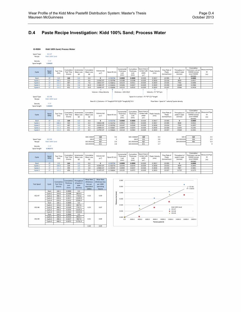
Wear Profile of the Kidd Mine Pastefill Distribution System: Master's Thesis Page D.4 Maureen McGuinness October 2013
D.4 Paste Recipe Investigation: Kidd 100% Sand; Process Water
KI-R004 Kidd 100% Sand; Process Water
Spool Type X52 #7
Recipe Kidd 100% Sand
Density 7.77
Spool length 0.06425
CycleSpool RPM
Test Time (hrs)
Cumulative Test Time
(hours)
Incremental Mass Loss
(g)
Cumulative Mass Loss
(g)
Volume lost
(m3)
Spool ID (m)
Incremental Thickness
Lost(mm)
Cumulative Thickness
Lost(mm)
Spool Area in contact with
paste
(m2)
Paste Velocity (m/s)
Flow Rate of Paste
(tonnes/hour)
Throughput of paste in pipe
(tonnes)
Cumulative Thickness Lost per
100000 tonnes(mm/100000
tonnes)
Measured Pipe
ID
(m)
Start 37 0.0 160 0.0 0.0 0 0.155750 0.0000 0.0000 0.0105 0.3017 23.905 0 0.0000
Cycle 1 37 160.1 325 4.6 4.6 5.920E-07 0.155788 0.0188 0.0188 0.0105 0.3018 23.916 3829 0.4917
Cycle 2 37 164.5 487 3.0 7.6 3.861E-07 0.155812 0.0123 0.0311 0.0105 0.3019 23.924 7765 0.4006
Cycle 3 37 161.9 651 2.6 10.2 3.346E-07 0.155833 0.0106 0.0417 0.0105 0.3019 23.930 11640 0.3586
Cycle 4 37 164.0 651 2.8 13.0 3.604E-07 0.155856 0.0115 0.0532 0.0105 0.3019 23.937 15566 0.3418
Volume = Mass/density thickness = (OD-ID)/2 Velocity = PI *ID*rpm
Spool Type X52 #8 Spool A in contact = PI *ID*1/3 *length
Recipe Kidd 100% Sand
New ID =[ (Volume + PI *length/4*ID^2)/(PI *length/4)]^0.5 Flow Rate = Spool A * velocity*paste density
Density 7.77
Spool length 0.06403
CycleSpool RPM
Test Time (hrs)
Cumulative Test Time
(hours)
Incremental Mass Loss
(g)
Cumulative Mass Loss
(g)
Volume lost
(m3)
Spool ID (m)
Incremental Thickness
Lost(mm)
Cumulative Thickness
Lost(mm)
Spool Area in contact with
paste
(m2)
Paste Velocity (m/s)
Flow Rate of Paste
(tonnes/hour)
Throughput of paste in pipe
(tonnes)
Cumulative Thickness Lost per
100000 tonnes(mm/100000
tonnes)
Measured Pipe
ID
(m)
Start 37 0.0 160 0.0 0.0 0 0.155750 0.0000 0.0000 0.0105 0.3017 23.905 0 0.0000
Cycle 1 37 160.1 325 0.3 0.3 3.861E-08 0.155752 0.0012 0.0012 0.0105 0.3017 23.905 3828 0.0321
Cycle 2 37 164.5 487 3.6 3.9 4.633E-07 0.155782 0.0147 0.0160 0.0105 0.3018 23.914 7762 0.2057
Cycle 3 37 161.9 651 2.3 6.2 2.960E-07 0.155801 0.0094 0.0254 0.0105 0.3018 23.920 11635 0.2181
Cycle 4 37 164.0 651 2.7 8.9 3.475E-07 0.155823 0.0110 0.0364 0.0105 0.3019 23.927 15560 0.2341
160.116667 160 4.6 160.1166667 160 0.3 164.5 164 3.5
Spool Type X52 #9 164.5 325 3 164.5 325 3.6 161.9333333 326 2.3
Recipe Kidd 100% Sand 161.933333 487 2.6 161.9333333 487 2.3 164.0333333 490 3.3
164.033333 651 2.8 164.0333333 651 2.7 0
Density 7.77
Spool length 0.062575
CycleSpool RPM
Test Time (hrs)
Cumulative Test Time
(hours)
Incremental Mass Loss
(g)
Cumulative Mass Loss
(g)
Volume lost
(m3)
Spool ID (m)
Incremental Thickness
Lost(mm)
Cumulative Thickness
Lost(mm)
Spool Area in contact with
paste
(m2)
Paste Velocity (m/s)
Flow Rate of Paste
(tonnes/hour)
Throughput of paste in pipe
(tonnes)
Cumulative Thickness Lost per
100000 tonnes(mm/100000
tonnes)
Measured Pipe
ID
(m)
Start 37 0.0 164 0.0 0.0 0 0.155750 0.0000 0.0000 0.0105 0.3017 23.905 0 0.0000
Cycle 1 37 164.5 326 3.5 3.5 4.505E-07 0.155779 0.0143 0.0143 0.0105 0.3018 23.913 3934 0.3642
Cycle 2 37 161.9 490 2.3 5.8 2.960E-07 0.155797 0.0094 0.0237 0.0105 0.3018 23.919 7807 0.3041
Cycle 3 37 164.0 490 3.3 9.1 4.247E-07 0.155824 0.0135 0.0372 0.0105 0.3019 23.927 11732 0.3175
Test Spool Cycle
Cumulative
Test Time
(hours)
Cumulative
Thickness
Lost
(mm)
Throughput
of paste in
pipe
(tonnes)
Wear Rate
(thickness
loss per
equivalent
100kt)
Wear Rate
(thickness loss
per 1000
operating
hours)
Start 160.1 0.0000 0.0
Cycle 1 324.6 0.0188 3829.4
Cycle 2 486.5 0.0311 7764.8
Cycle 3 650.6 0.0417 11639.9
Cycle 4 650.6 0.0532 15566.4
Start 160.1 0.0000 0.0
Cycle 1 324.6 0.0012 3827.6
Cycle 2 486.5 0.0160 7761.5
Cycle 3 650.6 0.0254 11635.0
Cycle 4 650.6 0.0364 15559.8
Start 164.5 0.0000 0.0
Cycle 1 326.4 0.0143 3933.7
Cycle 2 490.5 0.0237 7807.0
Cycle 3 490.5 0.0372 11731.9
0.30 0.09
0.09
0.07
0.09
X52 #7
X52 #8
X52 #9
0.33
0.25
0.31
y = 3E-06xR² = 0.8543
0.000
0.010
0.020
0.030
0.040
0.050
0.060
0.0 2000.0 4000.0 6000.0 8000.0 10000.0 12000.0 14000.0 16000.0 18000.0
Thic
kne
ss lo
st (
mm
)
Tonnes paste (t)
Kidd 100% SandX52 #7
X52 #8X52 #9
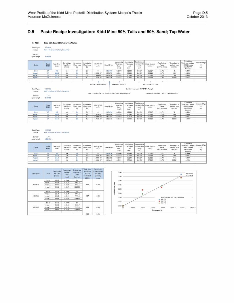
Wear Profile of the Kidd Mine Pastefill Distribution System: Master's Thesis Page D.5 Maureen McGuinness October 2013
D.5 Paste Recipe Investigation: Kidd Mine 50% Tails and 50% Sand; Tap Water
KI-R004 Kidd 50% Sand 50% Tails; Tap Water
Spool Type X52 #10
Recipe Kidd 50% Sand 50% Tails; Tap Water
Density 7.77
Spool length 0.06376
CycleSpool
RPM
Test Time
(hrs)
Cumulative
Test Time (hours)
Incremental
Mass Loss(g)
Cumulative
Mass Loss(g)
Volume lost
(m3)
Spool ID (m)
Incremental
Thickness
Lost(mm)
Cumulative
Thickness
Lost(mm)
Spool Area in contact with
paste
(m2)
Paste Velocity
(m/s)
Flow Rate of
Paste(tonnes/hour)
Throughput of
paste in pipe(tonnes)
Cumulative
Thickness Lost per
100000 tonnes(mm/100000
tonnes)
Measured Pipe
ID
(m)
Start 37 0.0 164 0.0 0.0 0 0.155750 0.0000 0.0000 0.0104 0.3017 23.722 0 0.0000
Cycle 1 37 164.5 326 3.5 3.5 4.505E-07 0.155779 0.0144 0.0144 0.0104 0.3018 23.731 3904 0.3698
Cycle 2 37 161.9 490 2.3 5.8 2.960E-07 0.155798 0.0095 0.0239 0.0104 0.3018 23.737 7748 0.3088
Cycle 3 37 164.0 490 3.3 9.1 4.247E-07 0.155825 0.0136 0.0375 0.0104 0.3019 23.745 11643 0.3224
Volume = Mass/density thickness = (OD-ID)/2 Velocity = PI *ID*rpm
Spool Type X52 #11 Spool A in contact = PI *ID*1/3 *length
Recipe Kidd 50% Sand 50% Tails; Tap Water
New ID =[ (Volume + PI *length/4*ID^2)/(PI *length/4)]^0.5 Flow Rate = Spool A * velocity*paste density
Density 7.77
Spool length 0.06403
CycleSpool RPM
Test Time (hrs)
Cumulative Test Time
(hours)
Incremental Mass Loss
(g)
Cumulative Mass Loss
(g)
Volume lost
(m3)
Spool ID (m)
Incremental
Thickness Lost
(mm)
Cumulative
Thickness Lost
(mm)
Spool Area in
contact with
paste
(m2)
Paste Velocity (m/s)
Flow Rate of Paste
(tonnes/hour)
Throughput of paste in pipe
(tonnes)
Cumulative
Thickness Lost per 100000 tonnes
(mm/100000
tonnes)
Measured Pipe
ID
(m)
Start 37 0.0 164 0.0 0.0 0 0.155750 0.0000 0.0000 0.0104 0.3017 23.722 0 0.0000
Cycle 1 37 164.5 326 4.6 4.6 5.920E-07 0.155788 0.0190 0.0190 0.0104 0.3018 23.734 3904 0.4860
Cycle 2 37 161.9 490 0.7 5.3 9.009E-08 0.155794 0.0029 0.0219 0.0104 0.3018 23.736 7748 0.2822
Cycle 3 37 164.0 490 2.9 8.2 3.732E-07 0.155818 0.0120 0.0338 0.0104 0.3019 23.743 11642 0.2905
Spool Type X52 #12
Recipe Kidd 50% Sand 50% Tails; Tap Water
Density 7.77
Spool length 0.062575
CycleSpool
RPM
Test Time
(hrs)
Cumulative
Test Time
(hours)
Incremental
Mass Loss
(g)
Cumulative
Mass Loss
(g)
Volume lost
(m3)
Spool ID (m)
Incremental Thickness
Lost
(mm)
Cumulative Thickness
Lost
(mm)
Spool Area in
contact with paste
(m2)
Paste Velocity
(m/s)
Flow Rate of
Paste
(tonnes/hour)
Throughput of
paste in pipe
(tonnes)
Cumulative Thickness Lost per
100000 tonnes
(mm/100000 tonnes)
Measured Pipe
ID
(m)
Start 37 0.0 164 0.0 0.0 0 0.155750 0.0000 0.0000 0.0104 0.3017 23.722 0 0.0000
Cycle 1 37 164.5 326 3.4 3.4 4.376E-07 0.155778 0.0140 0.0140 0.0104 0.3018 23.731 3904 0.3593
Cycle 2 37 161.9 490 2.4 5.8 3.089E-07 0.155798 0.0099 0.0239 0.0104 0.3018 23.737 7747 0.3088
Cycle 3 37 164.0 490 2.3 8.1 2.960E-07 0.155817 0.0095 0.0334 0.0104 0.3019 23.743 11642 0.2870
Test Spool Cycle
Cumulative
Test Time
(hours)
Cumulative
Thickness
Lost
(mm)
Throughput
of paste in
pipe
(tonnes)
Wear Rate
(thickness
loss per
equivalent
100kt)
Wear Rate
(thickness loss
per 1000
operating
hours)
Start 164.5 0.0000 0.0
Cycle 1 326.4 0.0144 3903.8
Cycle 2 490.5 0.0239 7747.5
Cycle 3 490.5 0.0375 11642.5
Start 164.5 0.0000 0.0
Cycle 1 326.4 0.0190 3904.2
Cycle 2 490.5 0.0219 7747.8
Cycle 3 490.5 0.0338 11642.4
Start 164.5 0.0000 0.0
Cycle 1 326.4 0.0140 3903.7
Cycle 2 490.5 0.0239 7747.5
Cycle 3 490.5 0.0334 11642.1
0.29 0.06
0.09
0.08
0.00
X52 #10
X52 #11
X52 #12
0.31
0.27
0.28
y = 3E-06x
R² = 0.9616
0.000
0.005
0.010
0.015
0.020
0.025
0.030
0.035
0.040
0.0 2000.0 4000.0 6000.0 8000.0 10000.0 12000.0 14000.0
Thic
kne
ss lo
st (
mm
)
Tonnes paste (t)
Kidd 50% Sand 50% Tails; Tap WaterX52 #10X52 #11X52 #12

Wear Profile of the Kidd Mine Pastefill Distribution System: Master's Thesis Page D.6 Maureen McGuinness October 2013
D.6 Statistical Analysis of Wear Test Results
Statistical analysis for the wear unit (mm/100 kt)
Two-Sample T-Test and CI: 50/50PW, 50/50TW Two-sample T for 50/50PW vs 50/50TW N Mean StDev SE Mean 50/50PW 3 0.2823 0.0246 0.014 50/50TW 3 0.2895 0.0233 0.013 Difference = mu (50/50PW) - mu (50/50TW) Estimate for difference: -0.0071 95% CI for difference: (-0.0693, 0.0551) T-Test of difference = 0 (vs not =): T-Value = -0.36 P-Value = 0.740 DF = 3
Two-Sample T-Test and CI: Tails only, Sand Only Two-sample T for Tails only vs Sand Only N Mean StDev SE Mean Tails only 3 0.3304 0.0475 0.027 Sand Only 3 0.2972 0.0428 0.025 Difference = mu (Tails only) - mu (Sand Only) Estimate for difference: 0.0333 95% CI for difference: (-0.0842, 0.1507)
50/50TW50/50PW100Tails100Sand
0.375
0.350
0.325
0.300
0.275
0.250
We
ar
Ra
te (
mm
/1
00
kt)

Wear Profile of the Kidd Mine Pastefill Distribution System: Master's Thesis Page D.7 Maureen McGuinness October 2013
T-Test of difference = 0 (vs not =): T-Value = 0.90 P-Value = 0.434 DF = 3
One-way ANOVA: Wear Rate (mm/100kt) versus Test Source DF SS MS F P Test 3 0.00408 0.00136 1.04 0.426 Error 8 0.01046 0.00131 Total 11 0.01454 S = 0.03617 R-Sq = 28.03% R-Sq(adj) = 1.04% Individual 95% CIs For Mean Based on Pooled StDev Level N Mean StDev -+---------+---------+---------+-------- 100Sand 3 0.29716 0.04278 (-----------*-----------) 100Tails 3 0.33045 0.04749 (-----------*-----------) 50/50PW 3 0.28233 0.02460 (-----------*-----------) 50/50TW 3 0.28945 0.02327 (-----------*-----------) -+---------+---------+---------+-------- 0.240 0.280 0.320 0.360 Pooled StDev = 0.03617
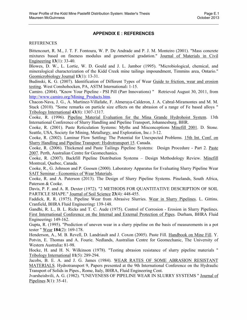
Wear Profile of the Kidd Mine Pastefill Distribution System: Master's Thesis Page E.1 Maureen McGuinness October 2013
APPENDIX E : REFERENCES
REFERENCES
Bittencourt, R. M., J. T. F. Fontoura, W. P. De Andrade and P. J. M. Monteiro (2001). "Mass concrete mixtures based on fineness modulus and geometrical gradation." Journal of Materials in Civil Engineering 13(1): 33-40. Blowes, D. W., L. Lortie, W. D. Gould and J. L. Jambor (1995). "Microbiological, chemical, and mineralogical characterization of the Kidd Creek mine tailings impoundment, Timmins area, Ontario." Geomicrobiology Journal 13(1): 13-31. Budinski, K. G. (2007). Identification of Different Types of Wear Guide to friction, wear and erosion testing. West Conshohocken, PA, ASTM International: 1-15. Camiro. (2004). "Know Your Pipeline - PSI Pill (Parr Innovations) " Retrieved August 30, 2011, from http://www.camiro.org/Mining_Products.htm. Chacon-Nava, J. G., A. Martinez-Villafañe, F. Almeraya-Calderon, J. A. Cabral-Miramontes and M. M. Stack (2010). "Some remarks on particle size effects on the abrasion of a range of Fe based alloys " Tribology International 43(8): 1307-1317. Cooke, R. (1996). Pipeline Material Evaluation for the Mina Grande Hydrohoist System. 13th International Conference of Slurry Handling and Pipeline Transport, Johannesburg, BHR. Cooke, R. (2001). Paste Reticulation Systems: Myths and Misconceptions Minefill 2001. D. Stone. Seattle, USA, Society for Mining, Metallurgy, and Exploration, Inc.: 3-12. Cooke, R. (2002). Laminar Flow Settling: The Potential for Unexpected Problems. 15th Int. Conf. on Slurry Handling and Pipeline Transport: Hydrotransport 15. Canada. Cooke, R. (2006). Thickened and Paste Tailings Pipeline Systems: Design Procedure - Part 2. Paste 2007. Perth, Australian Centre for Geomechanics. Cooke, R. (2007). Backfill Pipeline Distribution Systems – Design Methodology Review. Minefill Montreal, Quebec, Canada. Cooke, R., G. Johnson and P. Goosen (2000). Laboratory Apparatus for Evaluating Slurry Pipeline Wear SAIT Seminar - Economics of Wear Materials. Cooke, R. and A. Paterson (2013). The Design of Slurry Pipeline Systems. Pinelands, South Africa, Paterson & Cooke. Davis, P. F. and A. R. Dexter (1972). "2 METHODS FOR QUANTITATIVE DESCRIPTION OF SOIL PARTICLE SHAPE." Journal of Soil Science 23(4): 448-455. Faddick, R. R. (1975). Pipeline Wear from Abrasive Slurries. Wear in Slurry Pipelines. L. Gittins. Cranfield, BHRA Fluid Engineering: 139-148. Gandhi, R. L., B. L. Ricks and T. C. Aude (1975). Control of Corrosion - Erosion in Slurry Pipelines. First International Conference on the Internal and External Protection of Pipes. Durham, BHRA Fluid Engineering: 149-162. Gupta, R. (1995). "Prediction of uneven wear in a slurry pipeline on the basis of measurements in a pot tester " Wear 184(2): 169-178. Henderson, A., M. B. Revell, D. Landriault and J. Coxon (2005). Paste Fill. Handbook on Mine Fill. Y. Potvin, E. Thomas and A. Fourie. Nedlands, Australian Centre for Geomechanic, The University of Western Australia: 81-98. Hocke, H. and H. N. Wilkinson (1978). "Testing abrasion resistance of slurry pipeline materials " Tribology International 11(5): 289-294. Jacobs, B. E. A. and J. G. James (1984). WEAR RATES OF SOME ABRASION RESISTANT MATERIALS. Hydrotransport 9, Papers presented at the 9th International Conference on the Hydraulic Transport of Solids in Pipes., Rome, Italy, BHRA, Fluid Engineering Cent. Jvarsheishvili, A. G. (1982). "UNEVENESS OF PIPELINE WEAR IN SLURRY SYSTEMS " Journal of Pipelines 3(1): 35-41.

Wear Profile of the Kidd Mine Pastefill Distribution System: Master's Thesis Page E.2 Maureen McGuinness October 2013
Landriault, D. and W. Lidkea (1993). Paste fill and high density slurry backfill. Proceedings of the International Congress on Mine Design, Aug 23 - 26 1993, Kingston, Ont, Canada, A.A. Balkema. Landriault, D. A., R. E. Brown and D. B. Counter (2000). "Paste backfill study for deep mining at Kidd Creek." CIM Bulletin 93(1036): 156-161. Lee, C. and E. Pieterse (2005). Commissioning and Operating Experience with a 400 t/h Paste Backfill System at Kidd Creek Mine Paste 2005 Proceedings of the Eighth International Seminar on Paste and Thickened Tailings R. J. a. S. Barrera. Santiago, Chile: 299-316. Lovchev, V. (2009). "Improvement and optimization of techniques for monitoring erosion-corrosion wear of equipment and pipelines at nuclear power stations " Thermal Engineering 56(2): 134-141. McGuinness, M. and R. Cooke (2011). Pipeline wear and the hydraulic performance of pastefill distribution systems: the Kidd Mine experience Minefill 2011 Proceeding of the 10th International Symposium on Mining with Backfill "Fill or Fail". Cape Town, South Africa 205-212. McGuinness, M. A. and C. Bruneau (2008). Pastefill Operation at Xstrata Copper – Kidd Mine Maintenance Engineering / Mine Operators' Conference MEMO 2008. Val d'Or, Quebec, CIM: 50-58. McKibben, M. J. and C. A. Shook (1991). Chapter 20: Erosive Wear of Pipeline Systems. Slurry Handling – Design of Solid-Liquid Systems. N. P. B. N. I. Heywood, Elsevier Science Publishers (Ltd): 399-413. Newman, V. (2010). Kidd Updated Wear Tracking. Timmins, Ontario, Xstrata Copper - Kidd Mine. Pashias, N., D. V. Boger, J. Summers and D. J. Glenister (1996). "A fifty cent rheometer for yield stress measurement." Journal of Rheology 40(6): 1179-1189. Patil, M. S., E. R. Deore, R. S. Jahagirdar and S. V. Patil (2011). Study of the parameters affecting erosion wear of ductile material in solid-liquid mixture. World Congress on Engineering 2011, WCE 2011, July 6, 2011 - July 8, 2011, London, United kingdom, Newswood Ltd. Rong, H., Z. Peng, Y. Hu, C. Wang, W. Yue, Z. Fu and X. Lin (2011). "Dependence of wear behaviors of hardmetal YG8B on coarse abrasive types and their slurry concentrations " Wear 271(7-8): 1156-1165. Shou, G. (2007). "Wear rate prediction for long distance slurry pipelines " HYDROTRANSPORT 17 - The 17th International Conference on the Hydraulic Transport of Solids ISSU(PAGE): 255-261. Steward, N. R. and A. J. S. Spearing (1992). "COMBATING PIPELINE WEAR - AN ADVANCING TECHNOLOGY " Journal of the South African Institute of Mining and Metallurgy 92(6): 149-157. Steward, N. R. and A. J. S. Spearing (1992). "THE PERFORMANCE OF BACKFILL PIPELINES " Journal of the South African Institute of Mining and Metallurgy 92(1): 27-34. Steward, N. R. and A. J. S. Spearing (1992). Wear of backfill pipelines in South Arican gold mines Simultaneus Convening of the 4th International Conference on Bulk Materials Storage, Handling and Transportation and the 7th International Symposium on Freight Pipelines, July 6, 1992 - July 8, 1992, Wollongong, Aust, Publ by IE Aust. Steward, N. R. and A. J. S. Spearing (1993). "THE EFFECT OF PARTICLE SHARPNESS ON THE WEAR OF BACKFILL PIPELINES " Journal of the South African Institute of Mining and Metallurgy 93(5): 129-134. Swanson, P. A. and A. F. Vetter (1985). "MEASUREMENT OF ABRASIVE PARTICLE SHAPE AND ITS EFFECT ON WEAR " ASLE transactions 28(2): 225-230. Truscott, G. F. (1975). A Literature Survey on Wear in Pipelines. Wear in Slurry Pipelines. Cranfield, BHRA Fluid Engineering: 50-68. Truscott, G. F. (1979). Wear in Pumps and Pipelines. Wear in Slurry Pipelines. Cranfield, BHRA Fluid Engineering: 1-22. Wang, X.-M., D-M. Zhang, and Q-I. Zhang (2011). Form and mechanism of abrasion in backfill drill-hole pipelines in deep mines Minefill 2011 Proceeding of the 10th International Symposium on Mining with Backfill "Fill or Fail". H. J. Ilgner. Cape Town, South Africa, The Southern African Insititute of Mining and Metallurgy, 2011: 213-220. White, A. (2013). Paste Strength Requirements at Kidd Mine. Timmins, Ontario, Xstrata Copper - Kidd Mine.

Wear Profile of the Kidd Mine Pastefill Distribution System: Master's Thesis Page E.3 Maureen McGuinness October 2013
Yu, T. (1983). "BACKFILL PRACTICE AND TECHNOLOGY AT KIDD CREEK MINES." CIM bulletin 76(856): 56-65.