Wealth Inequality and Intergenerational Linksusers.nber.org/~denardim/research/denardi.pdf · DE...

Review of Economic Studies (2004)71, 743–768 0034-6527/04/00300743$02.00c© 2004 The Review of Economic Studies Limited

Wealth Inequality andIntergenerational Links

MARIACRISTINA DE NARDIUniversity of Minnesota and Federal Reserve Bank of Minneapolis

First version received July2001; final version accepted June2003(Eds.)

Previous work has had difficulty generating household saving behaviour that makes the distributionof wealth much more concentrated than that of labour earnings, and that makes the richest households holdonto large amounts of wealth, even during very old age. I construct a quantitative, general equilibrium,overlapping-generations model in which parents and children are linked by accidental and voluntarybequests and by earnings ability. I show that voluntary bequests can explain the emergence of large estates,while accidental bequests alone cannot, and that adding earnings persistence within families increaseswealth concentration even more. I also show that the introduction of a bequest motive generates lifetimesavings profiles more consistent with the data.

1. INTRODUCTION

Several papers have documented the fact that the distribution of wealth is much moreconcentrated than that of labour earnings and that it is characterized by a tiny fraction ofhouseholds owning huge estates (see, for example,Dıaz-Gimenez, Quadrini and Rıos-Rull(1997), Davies and Shorrocks(2000)).

An extensive literature, both empirical and theoretical, shows that the transmission ofphysical and human capital from parents to children is a very important determinant ofhouseholds’ wealth and earnings ability (see, among others,Becker and Tomes(1979, 1986),Kotlikoff and Summers(1981), Mulligan (1997), Hurd and Smith(1999)). Moreover, manypapers argue that households with higher levels of lifetime income have higher saving rates,keep substantial amounts of assets (even during old age), and leave very large bequests (amongthese,Dynan, Skinner and Zeldes(1996), Lillard and Karoly(1997), Carroll (1998)).

In this paper I focus on the transmission of physical and human capital from parents tochildren and show that such intergenerational links can induce saving behaviour that generates adistribution of wealth that is much more concentrated than that of labour earnings and that alsomake the rich keep large amounts of assets in old age in order to leave bequests to descendants.

I adopt a computable, general equilibrium, incomplete-markets, life-cycle model in whichparents and their children are linked by bequests, both voluntary and accidental, and by thetransmission of earnings ability. The households save to self-insure against labour earningsshocks and life-span risk, for retirement, and possibly to leave bequests to their children. Icalibrate the model to match relevant features of the data and analyse its implications for wealthconcentration and saving behaviour.

I find that voluntary bequests can explain the emergence of large estates, which areoften accumulated in more than one generation, and characterize the upper tail of the wealthdistribution in the data. Accidental bequests alone, even if unequally distributed, do not generatemore wealth concentration.

The presence of a bequest motive also generates lifetime saving profiles more consistentwith the data: saving for precautionary purposes and saving for retirement are the primary factors

743

744 REVIEW OF ECONOMIC STUDIES

for wealth accumulation at the lower tail of the distribution, while saving to leave bequestssignificantly affects the shape of the upper tail.

Modelling bequests as a luxury good is key in matching both of these facts. The bequestmotive to save is thus stronger for the richest households, who, even when very old, keep someassets to leave to their children. The rich leave more wealth to their offspring, who, in turn, tend todo the same. This behaviour generates some large estates that are transmitted across generationsbecause of the voluntary bequests, while being quantitatively consistent with the elasticity of thesavings of the elderly to permanent income that has been estimated from microeconomic data(Altonji and Villanueva, 2002).

A human–capital link, through which children partially inherit the productivity of theirparents, generates an even more concentrated wealth distribution. More productive parentsaccumulate larger estates and leave larger bequests to their children, who, in turn, are moreproductive than average in the workplace.

As a further test of the model, I also calibrate it to Swedish data. The cross-countrycomparison between the U.S. and Sweden suggests that intergenerational links are also importantin economies where redistribution programmes are more prominent and there is less inequality.Even when I change only the smallest possible number of parameters to match key Swedish data,the model with both intergenerational links does a better job of reproducing wealth inequality inSweden. This is particularly interesting because in Sweden the very richest hold a smaller amountof total wealth than in the U.S., while the poorest hold even less wealth than in the U.S. As aresult, the Gini coefficient of Swedish wealth is close to that of the U.S. As I argue later on,the behaviour of the poorest is well explained in the model by a more generous social insurancenetwork in Sweden, while the bequest motive is quantitatively important in explaining the wealthaccumulation behaviour of the richest even in Sweden.

1.1. Contributions with respect to the literature

Among the earlier partial equilibrium, quantitative studies,Davies(1982) analyses the effectsof various factors, including bequests, on economic inequality in a one-period model withoutuncertainty. In his set-up one generation of parents cares about their children’s futureconsumption, and there is regression to the mean between parents’ and children’s earnings. Asa consequence, the income elasticity of bequests is high and inherited wealth is a major causeof wealth inequality. Compared toDavies(1982), I adopt a general equilibrium, overlapping-generations set-up, with lifetime and earnings uncertainty, in which the expectation of receivingbequests from the parents influences their children’s saving behaviour. I also study the impact ofvarious saving motives over the life cycle and their effects on accumulated wealth, and I modelboth accidental and voluntary bequests and their impact on wealth inequality.

Among the general equilibrium literature,Hubbard, Skinner and Zeldes(1995) focus onthe effects of social insurance programmes on the wealth holdings of poor people. My paper,instead, concentrates on the effect of intergenerational links, especially on the upper tail of thewealth distribution.

Gokhale, Kotlikoff, Sefton and Weale(1998) quantify the amount of intra-generationalwealth inequality for the 66-year-old households arising from inheritances in a life-cycle set-upwith random death and fertility, assortative mating and heterogeneous human capital. Familiesare assumed to have a constant per capita consumption profile (which results in a large aggregateflow of accidental bequests) and do not take into account expected bequests when makingconsumption and saving decisions. In contrast withGokhaleet al. (1998), and consistent withthe data, my model generates higher saving rates for people with higher lifetime income andage-savings profiles consistent with the empirical observations.

DE NARDI WEALTH INEQUALITY AND INTERGENERATIONAL LINKS 745

Huggett(1996) is interested in how much wealth inequality can be generated using a purelife-cycle model with earnings shocks and an uncertain life span. His model matches the U.S.Gini coefficient for wealth, but the concentration is obtained by having more people in the lowertail and a much thinner upper tail than observed in the actual wealth distribution. Compared toHuggett’s (1996) model, I add voluntary bequests and intergenerational transmission of ability.

Heer(2001) adopts a life-cycle model in which rich and poor people have different tastes forleaving bequests. The model in this paper does not rely on heterogeneous preferences and adoptsa richer earnings process, which matches earnings persistence (as measured in microeconomicdata-sets), and also generates a reasonable distribution of labour earnings in the population. Byincluding an intergenerational transmission of earnings ability and comparing two very differentcountries, this paper also sheds light on the relative contribution of various factors in generatingwealth concentration.

Krusell and Smith(1997) study an economy populated by infinitely lived dynasties that faceidiosyncratic income and preference shocks. They show that it is possible to find a stochasticprocess for the dynasties’ discount factor to match the cross-sectional distribution of wealth. Incontrast, I explicitly model the life-cycle structure and intergenerational links, calibrate them tothe data, and study the impact of each of these forces.

Castaneda, Dıaz-Gimenez and Rıos-Rull (2003) study a model populated by dynastichouseholds that have some life-cycle flavour: workers have a constant probability of retiringin each period, retirees face a constant probability of dying, and each generation cares aboutits own offspring.Quadrini (2000) constructs an infinitely lived agent model in which agentscan choose to be entrepreneurs. The simplified structures of these dynastic models do not allowproper accounting for the life-cycle pattern of savings and the role of bequests in generatingwealth inequality.

Recent work byLaitner(2001) mixes life-cycle and dynastic behaviour: all households savefor life-cycle purposes, but only some of them care about their own descendants. There are perfectannuity markets; therefore, all bequests are voluntary. There is no earnings risk over the life cycle;hence, no precautionary savings. The concentration in the upper tail of the wealth distribution ismatched by choosing the fraction of households that behave as a dynasty and also depends onthe assumptions on the distribution of wealth within the dynasty, which is indeterminate in themodel.

2. SOME FACTS ABOUT THE UNITED STATES AND SWEDEN

Including residential structures, plant and equipment, land and consumer durables in my measureof capital, the average capital-to-GDP ratio is about 3 for the U.S. during the 1959–1992 period1

(Auerbach and Kotlikoff, 1995).Sweden is a small open economy, so the appropriate ratio to look at for my purposes is the

wealth-to-income ratio, which is 1·7 (seeDomeij and Klein, 1998, p. 16, Table 42).Kotlikoff and Summers(1981) estimated that private transfers of wealth across generations

account for at least 80% of the current value of total wealth.Modigliani (1988) claimed, instead,that at least 80% of total wealth is due to life-cycle accumulation. The discrepancy betweenthese two estimates is related to whether the accrued interest on the transfers is attributed to life-cycle accumulation or inherited wealth, to whether consumer durables are treated as consumptionor saving, and to whether parental support for children over the age of 18 is classified asconsumption or as transfers.

1. The wealth-to-GDP ratio for the U.S. is remarkably close to the capital-to-GDP ratio, varying between 2·9 in1989 and 3·1 in 1991.


TABLE 1

Wealth

Capital or wealth Transfer Percentage wealth in the topoutput ratio wealth ratio Wealth Gini

1% 5% 20% 40% 60% 80%

U.S. data3·0 0·60 0·78 29 53 80 93 98 100

Swedish data1·7 >0·51 0·73 17 37 75 99 100 100

TABLE 2

Gross earnings

Percentage earnings in the topGinicoeff. 1% 5% 20% 40% 80%

U.S. data0·46 6 19 48 72 98

Swedish data0·40 4 15 42 68 98

A recent study byGale and Scholz(1994) uses direct data on transfers and bequests, andestimates intergenerational wealth transfers to account for at least 60%. This number includesbequests and inter vivos transfers (adjusted for underreporting), but not college payments, andaccrues interest to the intergenerational transfers.2

The ratio of inheritances to wealth for Sweden comes fromLaitner and Ohlsson(1997),who compute the current value of household inheritances in Sweden as a fraction of householdwealth. The Swedish data seem to be of lower quality than the U.S. data and do not includeinter vivos transfers. Hence, the numbers for Sweden are likely to be lower bounds for the actualnumbers.

The U.S. data on the wealth distribution are from the 1989 Survey of Finances (SCF) andrefer to households 25 years of age and older. The distribution for 1992 is very similar. Wealthincludes owner-occupied housing, other real estate, cash, financial securities, unincorporatedbusiness equity, insurance and pension cash surrender value, and is net of mortgages and otherdebt. For Sweden, the wealth distribution data refer to 1984–1985 (Palsson, 1993).

Table2 is computed using data from the Luxembourg Income Study (LIS) data-set, whichcollects income data-sets from various countries (based on the March Current Population Surveyfor the U.S.) and makes them comparable. The table is computed using data for householdswhose head is 25–60 years of age, and the definition of gross earnings includes wages,salaries and self-employment income.Tables1 and2 show that earnings display a much lowerconcentration than wealth.

Comparing earnings and wealth inequality across these two countries, we can see thatthe Swedish earnings distribution is less concentrated than the U.S. distribution, but the Ginicoefficient for wealth is close in the two countries (0·78 in the U.S. and 0·73 in Sweden). Thehigh Ginicoefficients for wealth result from different reasons. In the U.S. the richest 5% of people

2. In this paper accrued interest will be consistently attributed to intergenerational transfers, both in the data, andin the model-generated data.


hold a large fraction of total wealth, 53%, and the poorest 60% of the population hold 7% oftotal net worth. On the contrary, in Sweden the richest 5% of people do not hold as much of totalwealth, 37%, but the poorest 60% of people hold only 1% of total net worth. This may be dueto the fact that social security and unemployment benefits are more generous in Sweden than inthe U.S., and these social insurance programmes are a disincentive to save, especially for peoplewith low lifetime earnings. In fact, people for whom social security benefits are high comparedto their lifetime income will not save for retirement in the presence of a redistributive socialsecurity system. Moreover, if security nets (such as unemployment insurance) are substantial,precautionary savings will be lower.

3. THE MODEL

The economy is populated by an infinitely lived government and overlapping generations ofpeople, who may differ in their productivity levels. The members of successive generations arelinked by bequests and the children’s inheritance of part of their parent’s productivity. At age20 each person enters the model and starts consuming, working and paying labour and capitalincome taxes. At age 25 the consumer procreates. After retirement the agent no longer works butreceives social security benefits from the government and interest from accumulated assets. Thegovernment taxes labour earnings, capital income and estates and pays pensions to the retirees.

3.1. Demographics

During each model period, which is 5 years long, a continuum of people3 is born. I define aget = 1 as 20 years old, aget = 2 as 25 years old, and so on. After one model period, att = 2, theagent’s children are born, and four periods later (when the agent is 45 years old) the children are20 and start working. Since there are no inter vivos transfers in this model economy, all agentsstart off their working life with no wealth. Total population grows at a constant, exogenous rate(n), and each agent has the same number of children.4 The agents are retired att = tr = 10 (i.e.when they are 65 years old) and die for sure by the end of ageT = 14 (i.e. before turning 90years old). Fromt = tr − 1 (i.e.60 years of age) toT , each person faces a positive probability ofdying given by(1−st ). Since death is assumed to be certain after ageT , sT = 0. The assumptionthat people do not die before 60 years of age reduces computational time and does not influencethe results because the number of people dying between the ages of 20 and 60 is small.

Since I consider only stationary environments, the variables are indexed only by age,t , andthe index for time is left implicit.

3.2. Preferences and technology

Preferences are assumed to be time separable, with a constant discount factor. The utility fromconsumption in each period is given byu(ct ) = c1−σ

t /(1 − σ).The parents derive utility from leaving a bequest, net of estate taxes,bt to their children:

φ(bt ). This type of bequest motive has been calledwarm glow, and was first introduced byAndreoni(1989). Considering a more sophisticated form of altruism would increase the numberof state variables (already four in this set-up) and, in some cases, would generate strategic parent–child interaction.

3. In the theoretical sections, I use the terms “agent”, “person”, “consumer”, and “household” interchangeably.Each household is taken to be composed of one person and dependent children.

4. The number of children is thusn5 if n is the growth rate of the population over 5 years, orn25 if n is expressedin yearly terms.


In this economy all agents face the same exogenous age-efficiency profile,εt , during theirworking years. This profile is estimated from the data and recovers the fact that productive abilitychanges over the life cycle. Workers also face stochastic shocks to their productivity level. Theseshocks are represented by a Markov process{yt } defined on(Y,B(Y)) and characterized by atransition functionQy, whereY ⊂ <++ andB(Y) is the Borelσ -algebra onY. This Markovprocess is the same for all households. The total productivity of a worker of aget is given bythe product of the worker’s stochastic productivity in that period and the worker’s deterministicefficiency index at the same age:ytεt . The parent’s productivity shock at age 40 is transmittedto children at age 20 according to a transition functionQyh, defined on (Y,B(Y)). What thechildren inherit is only their first draw; from age 20 on, their productivityyt evolves stochasticallyaccording toQy.

I assume that children cannot observe directly their parent’s assets, but only their parent’sproductivity when the parent is 40 and the children are 15, that is, the period before they “leavehome” and start working. Based on this information, children infer the size of the bequest theyare likely to receive. I will discuss the relevance and the qualitative effects of relaxing all of theseassumptions inSection7.

The household can only invest in physical capital, at a rate of returnr . The depreciation rateis δ, so the gross-of-depreciation rate of return on capital isr + δ. I assume also that the agentsface borrowing constraints that do not allow them to hold negative assets at any time.

I assume that the U.S. is a closed economy with an aggregate production functionF(K , L) = AKα L1−α, whereK is aggregate capital andL is aggregate labour. I instead assumethat Sweden is a small open economy, so the interest rate net of taxes is taken as exogenous andequal to that of the U.S.

3.3. Government

The government taxes labour earnings, capital income and estates to finance the exogenous publicexpenditure and to provide pensions to the retired agents.

Labour earnings are taken as exogenous and calibrated to the data, matching the after-taxGini coefficient. Since the U.S. tax system is progressive, this Gini coefficient is lower than theone computed from pre-tax labour earnings. In the model, I introduce a constant tax rateτl inorder to balance the government budget, while all the progressive features of the tax system arealready reflected in the calibrated after-tax earnings distribution.

Income from capital is taxed at a flat rateτa. Estates larger than a given valueexb are taxedat rateτb on the amount in excess ofexb.

The structure of the social security system is the following: the retired agents receive alump-sum transfer from the government each period until they die. The amount of this transferis linked to the average earnings of a person in the economy.

3.4. The household’s recursive problem

I consider an environment in which, during each period, at-year-old agent chooses consumptionc and risk-free asset holdings for the next period,a′. For given prices, the state variables for anagent are denoted byx = (t, a, y, yp). These variables indicate, respectively, the agent’s age(t),the agent’s assets carried from the previous period(a), the agent’s current productivity processrealization(y) and the value of the agent’s parent’s productivity at age 40 until the agent inheritsand zero thereafter(yp). This last variable takes on two purposes. First, when it is positive, itis used to compute the probability distribution on bequests that the household expects from theparent. Second, it distinguishes the agents who have already inherited, for whom I setyp = 0,


from those who have not, for whomyp is strictly positive. The agents inherit bequests only oncein a lifetime, at a random date which depends on their parent’s death. Since there is no marketfor annuities, part of the bequests the child receives are accidental bequests, linked to the factthat people’s life span is uncertain and people therefore accumulate precautionary savings tooffset the life-span risk. The optimal decision rules are functions for consumption,c(x), and nextperiod’s asset holdings,a′(x), that solve the dynamic programming problem described below.

(i) From aget = 1 to aget = 3 (from 20 to 30 years of age), the agent works and willsurvive with certainty until the next period. Moreover, the agent does not expect to receivea bequest soon because his or her parent is younger than 60 and will survive at least onemore period for sure. Since the law of motion ofyp is dictated by the death probability ofthe parent, for this subperiodyp′

= yp. Thus,

V(t, a, y, yp) = maxc,a′{u(c) + βEt V(t + 1, a′, y′, yp)} (1)

subject to

c ≤ [1 + r (1 − τa)]a + (1 − τl )εt y (2)

a′= [1 + r (1 − τa)]a − c + (1 − τl )εt y. (3)

The interest rate on assets is denoted byr , and the evolution ofy′ is described by thetransition functionQy.

(ii) From t = 4 to t = 8 (from 35 to 55 years of age), the worker will survive for sure up tothe next period. However, the agent’s parent is at least 60 years old and faces a positiveprobability of dying at any period; hence, a bequest might be received at the beginning ofthe next period. LetI yp>0 be the indicator function foryp > 0; it is one ifyp > 0 and zerootherwise. Thus,

V(t, a, y, yp) = maxc,a′{u(c) + βEt V(t + 1, a′, y′, yp′)} (4)

subject to (2) and

a′= [1 + r (1 − τa)]a − c + (1 − τl )εt y + b′ I yp>0I yp′=0 (5)

yp′=

{yp with probabilityst+5

0 with probability(1 − st+5)(6)

whereEt is the conditional expectation based on the information available at timet .The conditional distribution of the bequest a person expects in the case of parental

death is denoted byµb(x; ·).5 In equilibrium this distribution must be consistent with theparent’s behaviour. Since the evolution of the state variableyp is dictated by the deathprocess of the parent,yp′ jumps to zero with probability 1− st+5. (Five periods is thedifference in age between parents and their children.) I assume the following processes tobe independent: the survival/death of the decision maker; the survival/death of the parent;the size of the bequest received from the parent, conditional on the parent dying; and thefuture labour earnings, conditional on the current earnings.

(iii) The subperiodtr − 1 (60 years old) is the period before retirement. The agent starts facinga positive probability of dying, in which case the agent derives utility from bequeathing hisor her assets. Define after-tax bequests asb(a′) = a′

− τb · max(0, a′− exb). Thus,

V(t, a, y, yp) = maxc,a′{u(c) + stβEt W(t + 1, a′) + (1 − st )φ(b(a′))} (7)

5. The probability distributionµb depends onx only throught andyp, not throughy.


where

φ(b) = φ1

(1 +

b

φ2

)1−σ

(8)

subject to (2), (5), and (6). The termφ1 reflects the parent’s concern about leaving bequeststo her children, whileφ2 measures the extent to which bequests are a luxury good.6

(iv) Fromtr to T (from 65 to 85) is the period after retirement. The agent does not inherit afterturning 65 because the agent’s parent is already dead at that time. Moreover, I assume thatpeople no longer work after retirement and live off pensions and interest. This implies thatI can drop two state variables from the retired people’s value function,y andyp, and thatthe only uncertainty the retired agents face is the time of their death:

W(t, a) = maxc,a′{u(c) + stβW(t + 1, a′) + (1 − st )φ(b(a′))} (9)

subject to (8) and

c ≤ [1 + r (1 − τa)]a + p (10)

a′= [1 + r (1 − τa)]a − c + p (11)

wherep is the pension payment from the government. The terminal period value functionW(T + 1, a) is set to equalφ(b(a)).

3.5. Definition of stationary equilibrium

A stationary equilibrium is given by

an interest rater and wage ratew,

allocationsc(x), a′(x),

government tax rates and transfers(τa, τl , τb, exb, p),

a family of probability distributions for bequestsµb(x; ·),

and a constant distribution of people over the state variablesx: m∗(x)

such that the following hold:

(i) Given the interest rate, the wage, government tax rates and transfers, and the expectedbequest distributionµb(x; ·), the functionsc(x) and a′(x) solve the above describedmaximization problem for a household with state variablesx.

(ii) The tax rateτl is chosen so that the government budget constraint balances at every period:

g =

∫[τara + τl εt y It<tr − pIt≥tr + τb(1 − st−1) · max(0, a′(x) − exb)]dm∗(x).

(iii) The invariant distribution of households over the state variables for this economy,m∗, is afixed point of the operatorRM defined inAppendixA.1: RMm∗

= m∗. I normalizem∗ sothatm∗(X) = 1, which implies thatm∗(χ) is the fraction of people alive that are in a stateχ ∈ X .

(iv) The U.S. is treated as a closed economy. Aggregate capitalK is given by∫

a dm∗(x).Aggregate effective labour is denoted byL. In equilibrium the price of each factor is equalto its marginal product.

6. Even with full altruism, preferences over bequests and consumption would not be homothetic. This is becausebequests add to the permanent income of the children, which is already positive.


Sweden is treated as a small open economy, therefore its prices are taken as exogenous.K is still given by

∫a dm∗(x), but it now represents the average wealth held by Swedish

citizens (in Sweden and abroad), which may differ from average capital present in Sweden(held by Swedish people and foreigners).

(v) The family of expected bequest distributionsµb(x; ·) is consistent with the bequests thatare actually left by the parents. SeeAppendix A.2 for a formal characterization of thisstatement.

4. THE EXPERIMENTS

To understand the quantitative importance of these intergenerational links, I construct severalsimulations. I start with an experiment in which the model is stripped of all intergenerationallinks: an overlapping-generations model with life-span and earnings uncertainty. The accidentalbequests left by the people who die prematurely are seized by the government and equallyredistributed to all people alive.7 The idea is to see how much wealth inequality can be generatedby the life-cycle structure when only life-span and earnings uncertainty are activated. In thesecond experiment unplanned bequests are distributed to the children of the deceased, ratherthan equally to everybody alive. This is meant to assess whether an unequal distribution ofestates is quantitatively important when all bequests are involuntary. The third experiment addsinheritance of ability to the second one. In the fourth experiment parents care about leavingbequests to their children, but there is no inheritance of ability. The fifth exercise activates boththe bequest motive and the parent’s productivity inheritance in order to evaluate the importanceof both intergenerational links jointly.

To be consistent across experiments, I use the same initial distribution of productivity for20-year-old workers in all simulations for a given country. To do so, for each country I computethe initial aggregate distribution of productivity implied by the experiment with inheritanceof productivity and use it to initialize all the 20-year-old workers in the simulations withoutproductivity inheritance.

5. CALIBRATION

I distinguish two sets of parameters: those that can be estimated independently of the model orare based on estimates provided by other studies (Table3), and those that I choose so that themodel-generated data match a given set of targets (Table4). AppendixA.3 provides more detailsabout the calibration.

Table3. The rate of population growth isn, g is government expenditures andτa is thecapital income tax.

For the U.S.,α is the share of income that goes to capital, which I fix at 0·36 (Prescott(1986), Cooley and Prescott(1995)) and A is the constant in the production function, which isnormalized so that the wage is equal to one when the capital–output ratio is 3. I take depreciationfor the U.S. to be 6% (Stokey and Rebelo, 1995). Since Sweden is modelled as an open economy,its prices are taken as given, and there is no production function to be modelled and calibrated.

The rater is the interest rate on capital, net of depreciation and gross of taxes. Given thecalibration for the U.S. production function, this interest rate is endogenous for the U.S., and

7. This exercise uses Huggett’s set-up but adapts it to the length of the periods and the productivity process thatI use throughout this paper in order to make the results comparable to the other simulations I run. I cannot use the sametime period and income process that Huggett uses, since the simulations with intergenerational links require a highernumber of state variables and the model would require huge computing resources to solve.


TABLE 3

Parameters estimated independently of the model orprovided by other studies

Parameter U.S. calibration Swedish calibration

n 1·2% yearly 0·8% yearlyg 18% of GDP 25% of GDPτa 20% 30%α 0·36 n/aδ 0·06 n/aA See text n/ar Endogenous 6·86%st Vector Vectorεt Vector Vectorρy 0·85 0·85

σ2y 0·30 0·1429

ρyh 0·677 0·677

σ2yh 0·37 0·1762σ 1·5 1·5

TABLE 4

Parameters used to match some features in the data

Calibrated parameter U.S. calibration Swedish calibration

β 0·95–0·97 0·95–0·97φ1 −9·5 −9·5φ2 11·6 11·6τb 10% 15%exb 40 years of average earnings 10 years of average earningsp 40% average earnings 47–50% average earnings

turns out to be 6%. I take the Swedish interest rate to be 6·86%, so that the interest rates net oftaxes in the two countries coincide, and normalize its wage to one.

Thest ’s are the vectors of conditional survival probabilities for people older than 60, andεt

is the age-efficiency profile vector.The logarithm of the productivity process is assumed to be an AR(1) with persistenceρy

and varianceσ 2y . For the U.S. these two parameters are estimated from panel study on income

dynamics (PSID) data, aggregated over 5 years in order to be consistent with the model period.8

The logarithm of the productivity inheritance process (foryp) is also assumed to be anAR(1) with persistenceρyh and varianceσ 2

yh. I takeρyh from Zimmerman(1992), and for the

U.S. I chooseσ 2yh to match a Gini coefficient of 0·44 for earnings. These assumptions generate

an increase in earnings inequality over the life cycle that is consistent with the data.The persistence of the productivity and productivity inheritance processes are assumed

to be the same in Sweden and the U.S.Bjorklund and Jantti (1997) estimate the degree ofintergenerational income mobility in Sweden and do not reject the hypothesis that it is the same asin the U.S. As for the variances, in Sweden more generous social insurance programmes partiallyinsure households from idiosyncratic shocks and decrease earnings inequality. (More so than inthe U.S.; seeDe Nardi, Ren and Wei, 2000.) To recover this effect, I reduce bothσy andσyh for

8. I am very grateful to Altonji and Villanueva for kindly providing me with these estimates (seeTableA.1 formore details).


Sweden to match a Gini coefficient for earnings of 0·33, while imposing that the ratio ofσy andσyh for Sweden be equal to the corresponding ratio for the U.S.

I take risk aversion,σ , to be the same in the U.S. and in Sweden. The value that I use inthe calibration is fromAttanasio, Banks, Meghir and Weber(1999) andGourinchas and Parker(2002), who estimate it using consumption data. This value falls in the range (1–3) commonlyused in the literature.

Table4. For the U.S., in each experiment I choose the discount factor,β, to match a capital–output ratio of 3. On a yearly basis,β turns out to be 0·97 in the simulation in which accidentalbequests are equally distributed, 0·96 in the two experiments with accidental bequests (one withand one without productivity inheritance) and 0·95 in the two simulations with bequest motives,with and without productivity inheritance.

I use φ1 to match a transfer wealth share of 60% in the U.S. simulation with bothintergenerational links.

Many people leave estates of little or no value: according toHurd and Smith(1999), theaverage bequest left by single decedents at the lowest 30-th percentile was $2000 (Asset andHealth Dynamics among the Oldest Old (AHEAD) data-set, 1993–1995). Median householdincome in 1994 was $32,264 (U.S. Census Website, CPS data). I chooseφ2 to match that ratioin the model with both links. Using the average bequest left by singles rather than the one for alldecedents (which turns out to be $10,000) is a more sensible choice because typically a survivingspouse inherits a share of the estate, which will be partly consumed before finally being left tothe couple’s children.

I choose to use the same parameter values forφ1 andφ2, τb andexb, in the simulations withbequest motive only or with both intergenerational links in order to disentangle the increase inwealth inequality due to the two links when the preference parameters for bequests and estatetaxation are the same.

The preference parameters for Sweden are assumed to be equal to those for the U.S.The rateτb is the tax rate on estates that exceed the exemption levelexb. For the U.S. I set

these parameters to match the observed ratio of estate tax revenues to GDP, and the proportionof estates that pay estate taxes, 1·5% in the experiment with both intergenerational links.

In Sweden taxes are paid on inheritances, rather than on estates. It is therefore more difficultthan in the U.S. to define the statutory exemption level. The combined choice ofτb and exb

matches the revenues from bequests and gift taxes as a fraction of GDP in the experiment withboth intergenerational links. I do sensitivity analysis on these parameters for Sweden and findthat the results do not vary significantly for reasonable values of these parameters.

Pensions,p: for each country, the social security replacement rates are chosen such thatthe ratios of government transfers to GDP generated by the model are consistent with the ratioreported in theCouncil of Economic Advisors(1998) for the U.S. and with the one (net oftaxes) reported inOrganisation for Economic Co-operation and Development(1999) for 1996(respectively, 7% and 12%). The implied replacement rate for the U.S. is 40%, across allexperiments, which is a number similar to that used in many papers on social security. Theimplied replacement rate for Sweden is 50% in the experiments without a bequest motive, and47% in the other two. Using the same replacement rate of 50% in all simulations for Swedenwould generate very similar wealth distributions and a marginally lower capital–output ratio.

6. RESULTS

Tables5 and6 summarize the results for the U.S. and Sweden.9

9. For all experiments I exclude 20-year-old people from the computations on the wealth distribution because Iassume that people start off with zero wealth, and hence I do not propose a theory of the distribution of wealth for them.


TABLE 5

Results for the U.S. calibration

Capital–output Transfer wealth Wealth Percentage wealth in the top Percentage with negativeratio ratio Gini 1% 5% 20% 40% 60% or zero wealth

U.S. data3·0 0·60 0·78 29 53 80 93 98 5·8–15·0

No intergenerational links, equal bequests to all3·0 0·67 0·67 7 27 69 90 98 17

No intergenerational links, unequal bequests to children3·0 0·38 0·68 7 27 69 91 99 17

One link: productivity inheritance3·0 0·38 0·69 8 29 70 92 99 17

One link: parent’s bequest motive3·0 0·55 0·74 14 37 76 95 100 19

Both links: parent’s bequest motive and productivity inheritance3·0 0·60 0·76 18 42 79 95 100 19

TABLE 6

Results for the Swedish calibration

Wealth–output Transfer wealth Wealth Percentage wealth in the top Percentage with negativeratio ratio Gini 1% 5% 20% 40% 60% or zero wealth

Swedish data1·7 >0·51 0·73 17 37 75 99 100 30

No intergenerational links, equal bequests to all2·0 0·73 0·67 7 26 68 90 98 22

No intergenerational links, unequal bequests to children1·9 0·42 0·69 7 28 71 93 99 26

One link: productivity inheritance1·9 0·43 0·70 8 30 72 93 100 28

One link: bequest motive1·5 0·46 0·74 9 32 76 96 100 33

Both links: bequest motive and productivity inheritance1·5 0·47 0·75 10 34 78 96 100 33

6.1. No intergenerational links

Line 2 in Table5 shows that an overlapping-generations model with no dynastic links and equaldistribution of bequests has serious difficulties in generating enough skewness to match the U.S.distribution of wealth. The lower tail of the wealth distribution is too fat, and its upper tail is fartoo thin.

The large number of people at low asset levels is a common problem of overlapping-generations models. The households are born without savings that could be used to absorbnegative productivity shocks; hence, all young consumers who get a bad productivity shock hitthe borrowing constraint. As households work and get older, they gradually accumulate assets for

To explain the data for 20-year-old people, a theory of inter vivos transfers would, in my opinion, be required. The 20year olds are also excluded from the U.S. data on the distribution.


20 30 40 50 60 70 80 900

1

2

3

4

5

6

7

Age

Wea

lth

FIGURE 1

U.S. wealth 0·1, 0·3, 0·5, 0·7, 0·9, 0·95 quantiles, by age. No links, equal bequests to all

self-insurance purposes and to finance consumption during retirement, and the fraction of peoplewith low wealth gradually declines until retirement.

As for the upper tail, the richest 1% and 5% of people in the model hold, respectively,only 7% and 27% of total assets, compared with 29% and 53% in the data. The householdssave to buffer against income shocks, for retirement, and to self-insure against the risk of havinga long life span. These saving motives are not sufficient to generate huge asset holdings forparameterizations of the relevant processes that are consistent with the data.

The overlapping-generations model with no intergenerational links also fails to recover theage–asset profile observed in the data. All households in the model economy (Figure1) run downtheir assets during retirement until they are left with zero wealth at the time we assume they diefor sure. This implies a much larger dissaving than observed in the data, especially for the richerhouseholds.Dynan et al. (1996) find that the richest retirees (defined as those in the richestquintile or in the top 5% or 1% of the lifetime income distribution) not only keep substantialamounts of assets at advanced ages, but also keep saving a larger fraction of their income thanthe poorest retirees. Based on their empirical findings, the authors argue, “The results clearlyrule out models that imply that saving is proportional to permanent income.” They argue furtherthat “These results suggest that in the top 1% (or top 5%) of the population the motives forsaving, in particular for bequests, might be different from their less affluent (but still high income)colleagues.”

The transfer–wealth ratio appears high for this simulation because all living agents receivea transfer every year, starting at age 20 (rather than at age 54 on average, as it happens with morerealistic timing of bequests), and this measure includes interest from received transfers. This biasbecomes clearer in line 3, which corresponds to the model economy in which accidental bequestsare distributed to the children of those who die. In this case, the measure declines from 0·67 to0·38, even though the aggregate amount of bequests left in every period is almost the same.

Compared to the U.S. calibration, households in the Swedish model economy face lessearnings uncertainty and a higher social security replacement rate. The first element reduces


precautionary saving, and the second one reduces life-cycle saving. Given that I assume Swedishpeople to be as patient as those in the U.S., the model predicts a lower wealth-to-GDP ratio thanin the U.S. The distribution of wealth shows that, even in Sweden, the basic version of the modelgenerates an upper tail of the wealth distribution which is too thin; the richest 1% of people holdonly 7% of total wealth, compared with 14% in the data. Unlike the results for the U.S. modeleconomy, the model for Sweden does not generate too many people at zero wealth.

Line 3 inTables5 and6 displays the experiment in which accidental bequests are inheritedby the children of the deceased, rather than being distributed equally to all living people.Comparing lines 2 and 3, we can see that distributing accidental bequests unequally, rather thanequally, does not significantly increase wealth concentration in either country. The intuition isthe following: some people in the economy inherit some wealth, other people do not, but nobodycares about leaving bequests. Without a bequest motive, even high-income households dissavequickly after retirement. The age–asset profiles for the various quantiles of the wealth distributionalmost coincide with those generated by the previous experiment. In this economy, the largebequests are the ones left by 65-year-old people who die prematurely. Older people, even if theywere rich at age 65, keep few assets and leave small or no bequests when they die at advancedages. The likelihood that several generations of the same family die around age 65 is very small.For this reason this model fails to generate the intergenerational transmission of large estatesobserved in the data.

6.2. With intergenerational links

Line 4 in Tables5 and 6 shows that introducing productivity inheritance in the model withaccidental bequests has small effects on wealth inequality. The fraction of total wealth held bythe richest 1% of people increases from 7% to 8% in both countries. More productive parentstend to have more productive children, who, on average, receive larger bequests. However, thiseffect is small because just inheriting a higher productivity level from their parents does not makepeople choose higher saving rates, which is the mechanism that leads to the accumulation of thelarge fortunes observed in the data.

Even if the parameters in the bequest function were not chosen to generate more wealthconcentration, we can see from line 5 inTables5 and 6 that the introduction of the bequestmotive leads to a large increase in the concentration of wealth. In the simulations for the U.S.,the fraction of total wealth held by the people in the upper tail of the distribution increasessignificantly. The richest 1% of the population holds 14% of total wealth, and the richest 5%holds 37% of total wealth. In the simulations for Sweden, including the bequest motive increasesthe share of wealth held by the richest 1% of people from 7% to 9% and increases the share heldby the top 5% from 26% to 32%.

The intuition for why this happens is that the introduction of a nonhomothetic bequestmotive makes bequests a luxury good. Households that either have high lifetime income orreceive large bequests, or both, choose a higher saving rate, build up large estates, and keepa significant amount of assets even at advanced ages. These households, therefore, are morelikely to leave large bequests when they die. This mechanism explains the emergence of thelarge estates that are accumulated by more than one generation of savers and are transmittedbecause of the desire to donate one’s children some wealth.

The age–asset profiles for various quantiles of the U.S. wealth distribution are displayed inFigure2. In this figure notice a substantial difference in the main motives that lead the householdsto save. The median household saves mostly for retirement: the peak in its wealth holdings occursat age 65, and if the household reaches the age of 85, it consumes all of its assets (before dyingat age 90) and does not leave any bequest. The median consumer leaves mostly unintended


20 30 40 50 60 70 80 900

1

2

3

4

5

6

7

Age

Wea

lth

FIGURE 2

U.S. wealth 0·1, 0·3, 0·5, 0·7, 0·9, 0·95 quantiles, by age. Experiment with bequest motive only

bequests. This becomes clearer when we compare the age–asset profiles for the poorest 10%,30%, and 50% with the model with no bequest motive (Figure1): the profiles are very close.

At the top of the wealth distribution, a significant part of wealth is accumulated in order toleave bequests, and large bequests are left even when the parents die in advanced age. Comparingthese top quantiles with those in the model with no intergenerational links, we see how theintroduction of a bequest motive produces an age–wealth profile for the retirees that is consistentwith Dynanet al.’s (1996) findings. This is another feature of the model that is not matched byconstruction, but should be seen as a test of the model and its calibration.

Line 6 in Tables5 and6 refers to the experiment in which both intergenerational links areactivated. This version of the model does an even better job of matching the observed skewness inasset holdings. In the simulations for the U.S., the richest 1% of the population holds 18% of totalwealth, up from 14% in the previous simulation, and the richest 5% holds 42% of total wealth,up from 37%. The intergenerational transmission of productivity helps further in matching thetop 20% of the wealth distribution for Sweden: the shares held by the richest 1%, 5% and 10%increase to 10%, 32% and 52%, respectively.

When both intergenerational links are present, parents and children are linked not onlyby the bequest the parent intends to leave to the children, but also through transmission ofproductivity. Success in the workforce is now correlated across generations, and more productiveparents accumulate larger estates and leave their bequests to their children who are, in turn, moreproductive than average in the workforce.

To further gauge the ability of the model to explain the households’ saving decisions, it isuseful to compare other implications of the model to the data. I now look at the estate distributionand the elasticity of bequests to permanent income.

Figure 3 displays the cumulative distribution of estates implied by the model and thedistribution thatHurd and Smith(1999) report from the AHEAD data for single decedents. Thesize of the estates is normalized by median household income. One parameter of the modelwas chosen so that the two distributions match at one point: the 30-th percentile. The estate


0 5 10 15 20 25 30

0·1

0·2

0·3

0·4

0·5

0·6

0·7

0·8

0·9

Estate size, normalized by median income

Perc

entil

es

FIGURE 3

Cumulative distribution of estates, solid= model, dash–dot= AHEAD data

distribution generated by the model actually compares very well to the AHEAD data until the70-th percentile of the estate distribution. From that point on, the model predicts larger bequeststhan those observed in the AHEAD data. The discrepancy is partly due to the fact that AHEADmisses some large estates. AsDavies and Shorrocks(2000) point out, over-sampling the rich isnecessary to obtain a good representation of the asset holdings of the richest.

The model’s implications about the elasticity of the old people’s savings to permanentincome are consistent with recent microeconomic estimates.Altonji and Villanueva(2002) useU.S. data from the PSID to estimate the effect of an increase of 1 dollar of permanent income onthe asset holdings of the 70-year-old people. They find that this effect is rather small. To checkwhether this can be consistent with a model with voluntary bequests such as mine, they run thesame regressions on the actual data and on data simulated using the models in this paper forthe U.S. They find that the effect of a dollar of permanent income on the old people’s savingsgenerated by my model with voluntary bequests is consistent with the magnitudes that theyestimate in the data.

Now look at some of the features generated by the model to better understand itsfunctioning.Figure4 displays the strictly positive range of the bequest distribution for a 40-year-old person, conditional on the person’s parent’s observed productivity level, should the parentdie during that period. At that age, the probabilities of receiving zero bequests are, respectively,54%, 27%, 4% and 0%, for people with parents in the lowest, second lowest, second highest andhighest productivity levels. The average bequests expected are, respectively, 3, 5, 10 and 21 yearsof average labour earnings. Even in the presence of a bequest motive, the parents run down theirassets after retirement, so the expected bequest declines. The fraction of people whose parentlives up to the final age of the model economy and who do not receive a positive bequest are97%, 95%, 90% and 56%, respectively. The average bequest that they expect at that point in lifeis about 1·4, 1·7, 2·6 and 6·6 years of average labour earnings.

Figure5 shows the strictly positive range of the bequest distribution for 40-year-old Swedishagents, should their parent die this period. For people whose parent was at the lowest productivitylevel at age 40, the average bequest is 0.6 years of average labour earnings, and the probability


0 1 2 3 4 5 6 7 80

0·01

0·02

0·03

0·04

0·05

0·06

0·07

0·08

0·09

0·1

Bequest size

Prob

abili

ty

FIGURE 4

U.S. calibration. Strictly positive range of the expected bequest distribution at age 40, conditional on the productivity ofthe parent

0 1 2 3 4 5 6 7 80

0·01

0·02

0·03

0·04

0·05

0·06

0·07

0·08

0·09

0·1

Bequest size

Prob

abili

ty

FIGURE 5

Swedish calibration. Strictly positive range of the expected bequest distribution at age 40, conditional on the productivityof the parent

of receiving no intergenerational transfer is 65%. For those whose parent was at the highestproductivity level at age 40, the average bequest is 9 years of average labour earnings, and theprobability of receiving no intergenerational transfer is 0%. Compared to the U.S. simulation,the average bequest size for all parents’ levels of ability is lower.

Figure6 compares the saving behaviour of the average U.S. agent who expects to receivesome bequest with the agent’s behaviour in the hypothetical case in which the agent does not


20 25 30 35 40 45 50 55 600·04

0·06

0·08

0·1

0·12

0·14

0·16

0·18

Age

Wea

lth

FIGURE 6

U.S. calibration. Saving rate for households who expect to inherit or not. Experiment with bequest motive only

expect to receive a bequest. The fact that a parent’s assets are not observable influences thesaving behaviour of people who have not yet inherited. Since in this economy children do notbecome orphans before age 40 and everybody attributes positive probability to receiving somebequest until their parent dies, the comparison starts for agents of age 40. For them, we cancompare the behaviour of people whose parent died and did not leave them any asset (thesechildren do not expect an inheritance anymore) with the behaviour of people who still expect toreceive something. The top line refers to the age–saving profile for the average agent in the casein which the agent does not expect to inherit. While the average expected bequest decreases overtime, because of parental asset decumulation, the probability of the parent’s death increases overtime. These two forces balance out, decreasing the saving rate by similar amounts over the lifecycle. The corresponding figure for Sweden is similar.

Figures7 and 8 show that in the simulations the wealth quantiles of the people who doreceive a bequest are significantly higher than those who do not get a positive transfer of wealthfrom their parent.

7. DISCUSSION OF THE ASSUMPTIONS

In order to make the model manageable and solvable, I have made several simplifyingassumptions. In this section I discuss the assumptions and their likely qualitative implications.

The assumption that children partially inherit their parents’ productivity is meant to recoverthe fact that education and human capital are closely related to the family background of eachperson.Becker and Tomes(1979, 1986) study the parents’ optimal investment decision inchildren’s human capital in a set-up in which human capital investment in children has decreasingreturns, while the return on physical capital is fixed. In this setting parents begin investing in theirchildren’s human capital and then invest in physical capital when the return from human capitalfalls below the return on physical capital. In the presence of borrowing constraints, the poorestfamilies only invest in their children, and they may not even be able to do so at the optimallevel. The richest families not only invest in their children’s human capital but also leave them


25 30 35 40 45 50 55 600

1

2

3

4

5

6

7

Age

Wea

lth

FIGURE 7

U.S. calibration. Wealth quantiles: 0·1, 0·25, 0·5, 0·75, 0·85, 0·95, conditional on not having inherited

25 30 35 40 45 50 55 600

1

2

3

4

5

6

7

Age

Wea

lth

FIGURE 8

U.S. calibration. Wealth quantiles: 0·1, 0·25, 0·5, 0·75, 0·85, 0·95, conditional on having inherited

physical capital. Poorer families will tend to have poorer children, thus generating persistence inthe lower end of the wealth distribution. At the upper tail of the distribution, rich children mightwant to save less because they expect large bequests. However, they will also be richer (becauseof their dominant income process and the bigger transfers they receive from their parents); hence,they might want to save more. At the aggregate level, this will increase or decrease persistenceat the upper end of the wealth distribution, depending on which effect dominates. Most likely, ifthe altruism toward their children is strong enough for the richer people, the desire to leave large


estates to children will offset the reduction in saving because of the large bequests received.Which effect dominates thus depends on how wealth affects savings at high levels of wealth.

As discussed previously, I made restrictive assumptions on the information available to thechildren on their parent’s wealth and income. These assumptions are made for computationalreasons but are also likely to affect the results. In particular, I expect the model in the currentversion to display fatter tails at both ends of the wealth distribution, compared with a modelin which the parent’s assets and income are observable by the child. With perfect observabilitychildren of poor parents will save more, since they are aware that no bequest will be left to them.In contrast, children of richer parents will save less. If wealth of poor parents is easier to measurethan wealth of rich parents, only the lower tail of the distribution of wealth would become thinner.

Another important assumption is that there are no inter vivos transfers. In the data thesetransfers often have a compensatory nature: parents tend to give when the children need moneythe most. This may happen when they go to college, start a new job, get married, buy a house,or get a sequence of bad shocks. This assumption is probably most relevant when children are20–35 years of age and are starting off on their own. Allowing for inter vivos transfers wouldhelp reduce the number of people at zero wealth, especially among the young.

I take fertility to be exogenous and independent of households’ income. If poorer familiestend to have more children, the amount of resources received by each child will be evenlower, thus exacerbating wealth inequality.Knowles(1999) constructs a two-period, overlapping-generations model with fertility choice, human capital investment, and voluntary bequests, andhe studies its implications for income and wealth inequality. The model is capable of matchingthe fact that higher-income households on average tend to have fewer children and shows thatfertility decisions can help in matching some features of income concentration. While this modeldoes not generate the observed concentration of wealth in the upper tail of its distribution, itwould be interesting to investigate the effect of differential fertility in a set-up similar to the oneused in this paper.

I assume labour earnings to be exogenous. This is a limitation for two reasons. First, laboursupply might respond to the expectation of receiving a large bequest. Second, the U.S. datashow a noticeable correlation between high wealth and entrepreneurial activity. Some householdsmight accumulate huge fortunes because they face high implicit rates of return, but they are notfree to borrow as much as they wish to exploit these investment opportunities. Such a channelcould be quantitatively important to fully account for the saving decisions of the very richest.Both of these mechanisms are left for future research.

I also assume that the probability of death is independent of wealth and ability. In the datathe richer and more able people tend to live longer (see, for example,Attanasio and Emerson,2001). Introducing heterogeneous mortality (or survival probabilities that depend on wealth orability) into the model would not change the features of the saving behaviour that are key indriving the results: poor people save primarily for self-insurance; richer people also save to leavebequests. Given reasonable assumptions on the life span, savings against life-span risk wouldremain a small fraction of total wealth for the richest people. Therefore, introducing differentialmortality in this model (and, hence, a different timing of bequests) would not have a significantimpact on wealth inequality, and on the upper tail of the distribution in particular.

The results I report in the paper do not make any adjustment on consumption and utilityfor the demographic changes the household is undergoing over time. SinceAttanasioet al.(1999) found demographics to be important in their set-up, I also experimented by using per-adult-equivalent scale consumption, depending on the children’s age. (I used some estimateskindly provided by Guglielmo Weber.) When I introduced this modification, while at the sametime adjusting the discount factor to obtain a comparable capital–output ratio, the results didnot change in a quantitatively significant way. The intuition is related to the key features of


saving behaviour that I just described. Moreover, in this model, the hump-shaped behaviour inconsumption and wealth is generated by the presence of borrowing constraints (which generatethe increasing part of the hump during youth) and age-dependent probability of death (whichgenerates the decreasing part of the hump after retirement).

APPENDIX

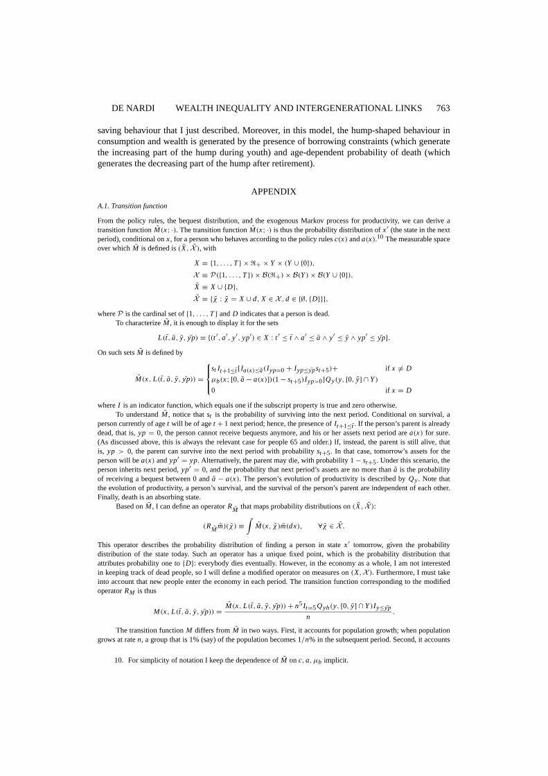
A.1. Transition function

From the policy rules, the bequest distribution, and the exogenous Markov process for productivity, we can derive atransition functionM(x; ·). The transition functionM(x; ·) is thus the probability distribution ofx′ (the state in the nextperiod), conditional onx, for a person who behaves according to the policy rulesc(x) anda(x).10 The measurable spaceover whichM is defined is(X, X ), with

X ≡ {1, . . . , T} × <+ × Y × (Y ∪ {0}),

X ≡ P({1, . . . , T}) × B(<+) × B(Y) × B(Y ∪ {0}),

X ≡ X ∪ {D},

X ≡ {χ : χ = X ∪ d, X ∈ X , d ∈ {∅, {D}}},

whereP is the cardinal set of{1, . . . , T} andD indicates that a person is dead.To characterizeM , it is enough to display it for the sets

L(t, a, y, yp) ≡ {(t ′, a′, y′, yp′) ∈ X : t ′ ≤ t ∧ a′≤ a ∧ y′

≤ y ∧ yp′≤ yp}.

On such setsM is defined by

M(x, L(t, a, y, yp)) =

st It+1≤t [Ia(x)≤a(Iyp=0 + Iyp≤ypst+5)+ if x 6= D

µb(x; [0, a − a(x)])(1 − st+5)Iyp>0]Qy(y, [0, y] ∩ Y)

0 if x = D

whereI is an indicator function, which equals one if the subscript property is true and zero otherwise.To understandM , notice thatst is the probability of surviving into the next period. Conditional on survival, a

person currently of aget will be of aget + 1 next period; hence, the presence ofIt+1≤t . If the person’s parent is alreadydead, that is,yp = 0, the person cannot receive bequests anymore, and his or her assets next period area(x) for sure.(As discussed above, this is always the relevant case for people 65 and older.) If, instead, the parent is still alive, thatis, yp > 0, the parent can survive into the next period with probabilityst+5. In that case, tomorrow’s assets for theperson will bea(x) andyp′

= yp. Alternatively, the parent may die, with probability 1− st+5. Under this scenario, theperson inherits next period,yp′

= 0, and the probability that next period’s assets are no more thana is the probabilityof receiving a bequest between 0 anda − a(x). The person’s evolution of productivity is described byQy. Note thatthe evolution of productivity, a person’s survival, and the survival of the person’s parent are independent of each other.Finally, death is an absorbing state.

Based onM , I can define an operatorRM that maps probability distributions on(X, X ):

(RM m)(χ) ≡

∫M(x, χ)m(dx), ∀χ ∈ X .

This operator describes the probability distribution of finding a person in statex′ tomorrow, given the probabilitydistribution of the state today. Such an operator has a unique fixed point, which is the probability distribution thatattributes probability one to{D}: everybody dies eventually. However, in the economy as a whole, I am not interestedin keeping track of dead people, so I will define a modified operator on measures on(X,X ). Furthermore, I must takeinto account that new people enter the economy in each period. The transition function corresponding to the modifiedoperatorRM is thus

M(x, L(t, a, y, yp)) =M(x, L(t, a, y, yp)) + n5 It=5Qyh(y, [0, y] ∩ Y)Iy≤yp

n.

The transition functionM differs from M in two ways. First, it accounts for population growth; when populationgrows at raten, a group that is 1% (say) of the population becomes 1/n% in the subsequent period. Second, it accounts

10. For simplicity of notation I keep the dependence ofM onc, a, µb implicit.


for births, which explains the second term in the numerator. If a person is 40 years old(t = 5), that person’s children(there aren5 of them) will enter the economy next period. All of those children have aget = 1 and zero assets.11 Theirstochastic productivity is inherited from their 40-year-old parent, according to the transition functionQyh; y (which ispart ofx) is their parent’s productivity at 40.

The operatorRM is thus defined as

(RM m)(χ) ≡

∫M(x, χ)m(dx) ∀χ ∈ X .

The operatorRM maps measures on(X,X ) into measures on(X,X ), but it does not necessarily map probabilitymeasures into probability measures. Unless the population is at a demographic steady state, the total measure of peoplealive may grow at a rate faster or slower thann, which implies that(RM m)(x) 6= 1 even ifm(x) = 1.

A.2. Consistency of bequest distributions

First define the marginal distribution of age and productivity in the population, which is a probability distribution on

({1, . . . , T} × Y,P({1, . . . , T}) × B(Y)) : m∗t,y(χt,y) ≡ m∗({x ∈ X : (t, y) ∈ χt,y}) ∀χt,y ∈ P({1, . . . , T}) × B(Y).

Define m∗(· | t, y) as the conditional distribution ofx given t and y. For any given(t, y), m∗(· | t, y) is aprobability distribution12 on (X,X ). For any setχ ∈ X , m∗(χ | t, y) is measurable with respect toP({1, . . . , T}) ×

B(Y) and is such that∫Xt,y

m∗(χ | t, y)m∗t,y(dt, dy) = m∗(χ) ∀χ ∈ X ∀χt,y ∈ P({1, . . . , T}) × B(Y).

The child observes the parent’s productivity at age 40. The conditional distribution of the characteristics of theparent at age 40, given a productivity levelyp, is13 m∗(· | t = 5, y = yp). I want the characteristics of the parent atlater ages, conditional on the parent’s productivity as of age 40 beingyp and conditional on not having died. Denote byl (· | t, yp) these conditional distributions. They can be obtained recursively as follows:l (χ | 5, yp) = m∗(χ | 5, yp)and

l (χ | t + 1, yp) ≡

∫x M(x, χ)l (dx | t, yp)

st.

The conditional distributionsl (· | t, yp) imply conditional distributions of assetsla(· | t, yp) on (<+,B(<+)),which are given by

la(χa | t, yp) ≡ l ({x ∈ X : a ∈ χa} | t, yp).

Since the probability of death is independent of productivity and assets, the distribution of assets that arebequeathed by dying parents is the same as the distribution of assets of surviving parents. I thus have

µb((t, a, y, yp); χa) = l

(a ∈ <+ : n5

(∏t−1

s=1ss

)−1 [aIa≤exb +

(exb +

a − exb(1 − τb)

)Ia>exb

]∈ χa | t + 5, yp

)× ∀χa ∈ B(<+) ∀a ∈ <+ ∀y, yp ∈ Y, t = 1, . . . , T − 5. (A.1)

In equation (A.1), I take into account the assumptions made before about the structure of bequest taxation and theassumption that the bequest is distributed evenly among surviving children.

I now need to defineµb whent = T − 4, which is the last age at which a person can inherit. Since there are nosurvivors at ageT + 1, I cannot use the survivor’s assets to compute the assets that are bequeathed. Instead, I use thepolicy functiona(x) to define

la(χa | T + 1, yp) ≡

∫X

Ia(x)∈χa l (dx | T, yp) ∀χa ∈ B(<+).

With this definition, equation (A.1) can be extended tot = T − 4 as well. Equation (A.1) is thus the formal requirementof consistency onµb.

11. Sincet ≥ 1 anda ≥ 0, I do not need to includeI1≤t and I0≤t .12. The conditional distribution{m∗(χ | t, y)} is uniquely defined up to sets ofm∗

t,y-measure zero.13. I useyp to distinguish from bothy andyp: yp plays the role of productivity for the parent (state variabley)

and the parent’s productivity for the child (state variableyp).


TABLE A.1

Log earnings persistence and variance

SpecificationL.H.S. variable 1 2 3 4

Husband’s earnings Persistence 0·92 0·91 0·87 0·86Variance 0·41 0·41 0·31 0·30

Husband’s earnings Persistence 0·90 0·89 0·84 0·81plus wife’s earnings Variance 0·38 0·36 0·29 0·27

Husband’s earnings Persistence 0·94 0·94 0·88 0·87plus unempl. insurance Variance 0·41 0·38 0·32 0·31plus workmen’s compensation

Husband’s earnings Persistence 0·92 0·90 0·85 0·80plus wife’s earnings Variance 0·38 0·36 0·30 0·27plus unempl. insuranceplus workmen’s compensation

A.3. More on the calibration

Survival probabilities. In the calibration of the U.S. economy, I use the mortality probabilities of people born in1965 (which are for the most part projected, since these people are still young) provided byBell, Wade and Goss(1992).The Statistics Sweden(1997) provides the mortality probabilities for people at various ages in 1991–1995. Since lifeexpectancy is increasing, the Swedish data underestimate the life expectancy at the various ages with respect to the onefaced by people born in 1965 in Sweden. To correct for this problem, I use the U.S. data to compute the relative increasein life expectancy for the relevant period. I then correct the Swedish data assuming that the increase in life expectancyis the same in the two countries. However, as a check, I also use the U.S. conditional probabilities in the simulation ofthe Swedish economy. It turns out that this has a negligible impact on the results even if the life expectancy of Swedishpeople is about 3 years longer than that of U.S. people.

Age-efficiency profile vectorεt . I assume it to be the same in both countries. Its source isHansen(1993).

The rates of population growth, n, are set to the respective average population growth from 1950 to 1997 for eachcountry (Council of Economic Advisors(1998), Organisation for Economic Co-operation and Development(1999)).

The ratio of g (total government expenditure and gross investment, excluding transfers—which includes federal,state and local for the U.S.) to GDP comes from theCouncil of Economic Advisors(1998) andOrganisation for EconomicCo-operation and Development(1999) for 1996.

The capital income taxτa (computed byKotlikoff, Smetters and Walliser, 1999for the U.S.) is equal to a flat taxrate of 30% in Sweden (Statistics Sweden, Website:http://www.scb.se/indexeng.asp).Estimates for thelog income processusing PSID income data aggregated over 5 years were very kindly provided byAltonji and Villanueva. The regressions were run as follows.Specification 1: Regressors are year dummies (take value 1 if the year is the first of a period of five) and a fourth-orderpolynomial in age, in differences from 40.Specification 2: Same regressors as in (1), plus an extra intercept for nonwhite.Specification 3: Same regressors as in (2), plus dummies for less than 5 years of schooling, more than 5 and less than 8,more than 8 and less than 11, college dropout, college, and more than college.Specification 4: Same regressors as in (3), plus intercept for not married, whether there are children in the household,and the number of children.

The estimates for persistence and variance in the upper half of the table are based on the sample of male heads ofhousehold in the PSID for the period 1968–1997. The PSID was divided in equally spaced 5-year periods, and incomewas aggregated within those cells. Only complete income spells of 5 years were used starting in 1968, 1973, 1978, 1983and 1993.

The estimates in the lower half of the table are based on a sample of males in the PSID for the period 1978–1997,given that questions about the exact amount of unemployment insurance and workmen’s compensation are only availablefrom 1977 on. Income from both unemployment insurance and workmen’s compensation are asked of husband and wife.

In all specifications, observations with earnings below five times 900 dollars (from 1993) are dropped. The varianceis taken from the pooled cross-section and time series variation of the prediction errors in the corresponding regression.

http://www.scb.se/indexeng.asp


TABLE A.2

Earnings

Percentage earnings in the topGinicoeff. 5% 10% 20% 40% 60% 80%

U.S. earnings data0·46 19 30 48 72 89 98

U.S. earnings+ social insurance transfers0·44 19 30 47 71 88 97

U.S. simulated earnings0·44 15 30 50 73 87 96

Swedish earnings data0·40 15 25 42 68 86 98

Swedish earnings+ social insurance transfers0·33 13 22 37 62 80 94

Swedish simulated earnings0·33 12 24 40 65 81 93

In my calibration for the U.S., I choose the persistence and variance parameters from the regression that includeslog earnings of the husband, earnings of the wife, and transfers and that pertain to the third specification, the one thataccounts for age, race and some education effects. This is a middle-of-the-range estimate among the relevant ones. Itshould be noted, however, that the range of the estimated parameters from the various regressions is rather tight.

I convert both the productivity and the productivity inheritance processes to four-state discrete Markov chainsaccording toTauchen and Hussey(1991). Since I want the possible realizations for the initial inherited productivity levelto be the same as the possible realizations for productivity during the lifetime, I choose the quadrature points jointly forthe two processes. The resulting gridpoints for the productivity processy for the U.S. and for Sweden are, respectively:[0·2594, 0·6513, 1·5355, 3·8547] and[0·3941, 0·7438, 1·3444, 2·5373]. Given the assumptions on the parameters of theprocesses, the transition matricesQy andQyh for the U.S. and Sweden are the same, and are given, respectively, by

0·7132 0·2764 0·0104 0·00000·1467 0·6268 0·2210 0·00550·0055 0·2210 0·6268 0·14670·0000 0·0104 0·2764 0·7132

0·5257 0·4228 0·0509 0·00070·1461 0·5538 0·2825 0·01760·0176 0·2825 0·5538 0·14610·0007 0·0509 0·4228 0·5257

·

TableA.2 reports data on earnings distributions for the U.S. and Sweden, respectively, and compares them with theearnings distributions used in the model. The tables are computed using data for households whose head is 25–60 years ofage. For each country the first row refers to gross earnings (which include wages, salaries, and self-employment income);the second row adds social insurance transfers to gross earnings; while the third row reports the earnings distributionimplied by the model.

Estate taxes. According to U.S. law, each individual can make an unlimited number of tax-free gifts of $10,000 orless per year, per recipient; therefore, a married couple can transfer $20,000 per year to each child, or other beneficiary.For larger gifts and estates, there is aunified credit, that is, a credit received by the estate of each deceased, againstlifetime estate and gift taxes. For the period between 1987 and 1997, each taxpayer received a tax credit that eliminatedestate tax liabilities on estates valued at less than $600,000. The marginal tax rate applicable to estates and lifetime giftsabove that threshold is progressive, starting from 37% (Poterba, 1998). However, the revenue from estate taxes is verylow (on the order of 0·2% of GDP in 1985–1997) because there are many effective ways to avoid such taxes (see,e.g.Aaron and Munnell(1992)). Moreover, only about 1·5% of decedents pay estate taxes. Therefore, in the model I setexbto be 40 times the median income andτb to be 10% to match the observed ratio of estate tax revenues to GDP and theproportion of estates that pay estate taxes. I discuss the sensitivity of the model to the choice of these two parameters


when describing the results. For Sweden, I take the effective tax rate to be higher than that for the U.S., 15%, andthe exemption level to be lower, 10 years of average labour earnings. In Sweden taxes are paid on inheritances, ratherthan on estates, and the revenue from inheritance and gift taxes is approximately 0·1% of GDP. The statutory tax ratefor children’s inheritance is higher than in the U.S. (for the first bracket it is about 50%) and the exemption level ismuch lower (on the order of $5000), but there are legal ways, for example, bequeathing an apartment or a large firm, ofobtaining a much larger exemption level. It is therefore more difficult than in the U.S. to define the statutory exemptionlevel. The combined choice ofτb andexb matches the revenues from bequests and gift taxes.

Acknowledgements. I am grateful to Joe Altonji, Orazio Attanasio, Lisa Barrow, Marco Bassetto, Gary S. Becker,Marco Cagetti, Lars P. Hansen, Tim Kehoe, Jose A. Scheinkman, Jenni Schoppers, Ernesto Villanueva, GuglielmoWeber, three anonymous referees, and especially Thomas J. Sargent for helpful comments and suggestions. I thankthe participants at seminars at many institutions for comments, and Martin Floden, Paul Klein and David Domeij fordiscussions about the Swedish data. All errors are my own. All views expressed herein are those of the author and notnecessarily those of the Federal Reserve Bank of Minneapolis or the Federal Reserve System.

REFERENCESAARON, H. J. and MUNNELL, A. H. (1992), “Reassessing the Role for Wealth Transfer Taxes”,National Tax Journal,

45 (2), 119–143.ALTONJI, J. G. and VILLANUEVA, E. (2002), “The Effect of Parental Income on Wealth and Bequests” (Mimeo,

Northwestern University).ANDREONI, J. (1989), “Giving with Impure Altruism: Applications to Charity and Ricardian Equivalence”,Journal of

Political Economy, 97, 1447–1458.ATTANASIO, O. P., BANKS, J., MEGHIR, C. and WEBER, G. (1999), “Humps and Bumps in Lifetime Consumption”,

Journal of Business and Economic Statistics, 17 (1), 22–35.ATTANASIO, O. P. and EMERSON, C. (2001), “Differential Mortaility in the UK” (Mimeo, University College

London).AUERBACH, A. J. and KOTLIKOFF, L. J. (1995)Macroeconomics: An Integrated Approach(Cincinnati: South-Western

College).BECKER, G. S. and TOMES, N. (1979), “An Equilibrium Theory of the Distribution of Income and Intergenerational

Mobility”, Journal of Political Economy, 87 (6), 1153–1189.BECKER, G. S. and TOMES, N. (1986), “Human Capital and the Rise and Fall of Families”,Journal of Labor Economics,

4 (3), 1–39.BELL, F. C., WADE, A. H. and GOSS, S. C. (1992)Life Tables for the United States Social Security Area: 1900–2080

(Social Security Administration, Office of the Actuary).BJORKLUND, A. and JANTTI, M. (1997), “Intergenerational Income Mobility in Sweden Compared to the United

States”,American Economic Review, 87 (5), 1009–1018.CARROLL, C. D. (1998), “Why Do the Rich Save So Much?” (Working Paper 6549, National Bureau of Economic

Research).CASTANEDA, A., DIAZ-GIM ENEZ, J. and RIOS-RULL, J.-V. (2003), “Accounting for U.S. Earnings and Wealth

Inequality”,Journal of Political Economy3 (4), 818–857.COOLEY, T. F. and PRESCOTT, E. C. (1995), “Economic Growth and Business Cycles”, in T. F. Cooley (ed.)Frontiers

of Business Cycle Research(Princeton, NJ: Princeton University Press) 1–38.COUNCIL OF ECONOMIC ADVISORS (1998)Economic Report of the President(Washington: United States

Government Printing Office).DAVIES, J. B. (1982), “The Relative Impact of Inheritance and Other Factors on Economic Inequality”,Quarterly Journal

of Economics, 9 (3), 471–498.DAVIES, J. B. and SHORROCKS, A. F. (2000), “The Distribution of Wealth”, in A. B. Atkinson and F. Bourguignon

(eds.)Handbook of Income Distribution, Handbooks in Economics, Vol. 16 (Amsterdam: Elsevier Science; NewYork and Oxford: North-Holland) 605–675.

DE NARDI, M., REN, L. and WEI, C. (2000), “Income Inequality and Redistribution in Five Countries”,Federal ReserveBank of Chicago Economic Perspectives, 24 (2), 2–20.

DIAZ-GIM ENEZ, J., QUADRINI, V. and RIOS-RULL, J.-V. (1997), “Dimensions of Inequality: Facts on theU.S. Distributions of Earnings, Income and Wealth”,Federal Reserve Bank of Minneapolis Quarterly Review,21 (2), 3–21.

DOMEIJ, D. and KLEIN, P. (1998), “Inequality of Income and Wealth in Sweden” (Mimeo).DYNAN, K. E., SKINNER, J. and ZELDES, S. P. (1996), “Do the Rich Save More?” (Manuscript, Board of Governors of

the Federal Reserve System).GALE, W. G. and SCHOLZ, J. K. (1994), “Intergenerational Transfers and the Accumulation of Wealth”,Journal of

Economic Perspectives, 8 (4), 145–160.GOKHALE, J., KOTLIKOFF, L. J., SEFTON, J. and WEALE, M. (1998), “Simulating the Transmission of Wealth

Inequality via Bequests” (Working Paper 9811, Federal Reserve Bank of Cleveland).GOURINCHAS, P.-O. and PARKER, J. A. (2002), “Consumption over the Life Cycle”,Econometrica, 70 (1), 47–89.HANSEN, G. D. (1993), “The Cyclical and Secular Behaviour of Labour Input: Comparing Efficiency Units and Hours

Worked”,Journal of Applied Econometrics, 8 (1), 71–80.


HEER, B. (2001), “Wealth Distribution and Optimal Inheritance Taxation in Life-Cycle Economies withIntergenerational Transfers”,Scandinavian Journal of Economics, 103(3), 445–465.

HUBBARD, R. G., SKINNER, J. and ZELDES, S. P. (1995), “Precautionary Saving and Social Insurance”,Journal ofPolitical Economy, 103(2), 360–399.

HUGGETT, M. (1996), “Wealth Distribution in Life-Cycle Economies”,Journal of Monetary Economics, 38 (3),469–494.

HURD, M. D. and SMITH, J. P. (1999), “Anticipated and Actual Bequests” (Working Paper No. 7380, National Bureauof Economic Research).

KNOWLES, J. (1999), “Can Parental Decisions Explain U.S. Income Inequality?” (Mimeo, Department of Economics,University of Pennsylvania).

KOTLIKOFF, L. J., SMETTERS, K. A. and WALLISER, J. (1999), “Privatizing Social Security in the UnitedStates: Comparing the Options”,Review of Economic Dynamics, 2 (3), 532–574.

KOTLIKOFF, L. J. and SUMMERS, L. H. (1981), “The Role of Intergenerational Transfers in Aggregate CapitalAccumulation”,Journal of Political Economy, 89 (4), 706–732.

KRUSELL, P. and SMITH, A. A. JR (1997), “Income and Wealth Heterogeneity, Portfolio Choice, and Equilibrium AssetReturns”,Macroeconomic Dynamics, 1 (2), 387–422.

LAITNER, J. (2001), “Secular Changes in Wealth Inequality and Inheritance”,The Economic Journal, 111 (474),691–721.

LAITNER, J. and OHLSSON, H. (1997), “Equality of Opportunity and Inheritance: A Comparison of Sweden and theU.S.” (Mimeo).

LILLARD, L. A. and KAROLY, L. A. (1997), “Income and Wealth Accumulation Over the Life-Cycle” (Manuscript,RAND Corporation).

MODIGLIANI, F. (1988), “Measuring the Contribution of Intergenerational Transfers to Total Wealth: Conceptual Issuesand Empirical Findings”, in D. Kessler and A. Masson (eds.)Modeling the Accumulation and Distribution of Wealth(Oxford: Clarendon Press).

MULLIGAN, C. B. (1997)Parental Priorities and Economic Inequality(Chicago: University of Chicago Press).ORGANISATION FOR ECONOMIC CO-OPERATION AND DEVELOPMENT (1999)OECD Economic Surveys,

1998–1999: Sweden(Paris and Washington, DC: OECD).PALSSON, A.-M. (1993), “Household Risk Taking and Wealth: Does Risk Taking Matter?”, in Daniel J. Slottje and

Edward N. Wolff (eds.)Research in Economic Inequality, Studies in the Distribution of Household Wealth, Vol. 4(JAI Press).

POTERBA, J. (1998), “Estate and Gift Taxes and Incentives for Inter Vivos Giving in the United States” (Working PaperNo. 6842, National Bureau of Economic Research).

PRESCOTT, E. C. (1986), “Theory ahead of Business Cycle Measurement”,Federal Reserve Bank of MinneapolisQuarterly Review, 10, 9–22.

QUADRINI, V. (2000), “Entrepreneurship, Saving and Social Mobility”,Review of Economic Dynamics, 3 (1), 1–40.STATISTICS SWEDEN (1997)Statistical Yearbook of Sweden, Statistics Sweden, Website:

http://www.scb.se/indexeng.asp.STOKEY, N. L. and REBELO, S. (1995), “Growth Effects of Flat-Tax Rates”,Journal of Political Economy, 103,

519–550.TAUCHEN, G. and HUSSEY, R. (1991), “Quadrature-Based Methods for Obtaining Approximate Solutions to Nonlinear

Asset Pricing Models”,Econometrica, 59 (2), 371–396.ZIMMERMAN, D. J. (1992), “Regression Toward Mediocrity in Economic Stature”,American Economic Review, 82 (3),

409–429.

http://www.scb.se/indexeng.asp

Wealth Inequality and Intergenerational Linksusers.nber.org/~denardim/research/denardi.pdf · DE...

Documents

Transcript of Wealth Inequality and Intergenerational Linksusers.nber.org/~denardim/research/denardi.pdf · DE...