Stability and persistence of intergenerational wealth ...wk2110/bin/WealthAcrossGen.pdf ·...

Intergenerational Wealth Formation over the Life Cycle:Evidence from Danish Wealth Records 1984-2013∗

Simon Halphen BoserupUniversity of Copenhagen

Wojciech KopczukColumbia University, CEPR, and NBER

Claus Thustrup KreinerUniversity of Copenhagen and CEPR

April 2017

Abstract

This paper provides novel insights on intergenerational wealth mobility and its relationshipto lifetime economic resources using thirty years of wealth records for the Danish population.Non-parametric evidence reveals an almost linear relationship between wealth ranks of childrenand parents, except at the very top of the distribution where the association is stronger. Theslope of the graph—the rank correlation—is 0.27 when both parents and children are in mid-life(age 45-50). We find a U-shaped pattern when looking at the rank correlation as a function ofchild age with a correlation of 0.35 when children move into adulthood (age 20), going down to0.17 in the mid-twenties and then moving gradually up again to 0.27 in the forties. After deathof parents, the correlation lies in the range 0.35-0.40. We provide a simple theoretical frame-work to understand intergenerational wealth mobility over the life-cycle. The theory explainsthe life-cycle pattern in measured wealth mobility through life-cycle patterns of transfers andearnings: wealthy parents make inter vivo transfers early in childrens’ life, their children havelow income in the twenties when investing in human capital, but a high permanent income and,finally, they receive large bequests. The U-shaped pattern requires that inter vivos transfersare quantitatively important and the increase in correlation at the receipt of bequests revealsthe quantitative importance of bequests. Our main interest is in the correlation across gener-ations in lifetime resources, which according to the theory may be captured by appropriatelyestimating intergenerational correlation in wealth. Our preferred estimate of the intergenera-tional correlation in lifetime resources is 0.25, which is significantly higher than the correlationof permanent incomes equal to 0.20.

∗This is a heavily revised version of a previous paper entitled “Intergenerational Wealth Mobility: Evidence fromDanish Wealth Records of Three Generations”. We are grateful for comments by Brant Abbott, Anders Björklund,Steven Haider, Søren Leth-Petersen, Martin David Munk, Emmanuel Saez, Daniel Waldenström, and participantsat a workshop on intergenerational mobility in Copenhagen, at the CEPR Public Policy Symposium, at the AEAmeeting, and at a number of seminar presentations. Benjamin Ly Serena provided excellent research assistance.Financial support from EPRN and the Danish Council for Independent Research (DFF – 1329-00046) is gratefullyacknowledged. Contact information: [email protected], [email protected], [email protected].

1 Introduction

Wealth formation and wealth inequality have received increasing attention academically and pub-

licly after the publication of the best-selling book by Thomas Piketty (2014). In this paper, we

provide novel insights on intergenerational wealth mobility over the life cycle using thirty years

of wealth records for the Danish population. A voluminous literature has analyzed how economic

well-being is related across generations by studying intergenerational linkages in outcomes such as

income, education, and health (see surveys by Solon 1999 and Black and Devereux 2011). Only

few studies exist on wealth (e.g., Charles and Hurst 2003) even though variation in wealth across

individuals at a given age level may be one of the best proxies for the variation in lifetime economic

resources and for the (in)equality of opportunities.1

Correlation of wealth across generations may be driven by mechanical correlation in innate

abilities across generations and deliberate parental investments in human capital of children as in

the standard theory of intergenerational income mobility by Becker and Tomes (1979, 1986), but

it may also reflect direct transfers of wealth from the previous generations made during life (inter

vivos) or at death (inheritance). Finally, decisions on consumption and saving are crucial for build-

ing up wealth and therefore for understanding correlation of wealth across generations (Stiglitz

1969). Thus, formation of wealth across generations may summarize many different intergenera-

tional channels important for individual well-being.

While correlation of wealth across generations may be of interest in its own right, we argue that

the main parameter of interest is the correlation in lifetime economic resources, which determines

overall consumption possibilities. Naturally, lifetime resources of an individual are related to—but

not directly observable from—income and wealth observed over the life-cycle.

We start our analysis by providing a simple theoretical framework to understand wealth for-

mation across generations over the life cycle and its relationship to lifetime resources. We build on

the standard Becker and Tomes (1979) with human capital investment extended to a multi-period

overlapping generations model with inter vivo wealth transfers and bequests. Each generation has

standard preferences over consumption that govern savings behavior, and makes wealth transfers

determined by simple joy-of-giving motives. This framework provides a number of interesting in-

sights. First, the intergenerational correlation in lifetime economic resources may be inferred from1Charles and Hurst (2003) use wealth data from the Panel Study of Income Dynamics (PSID) to estimate the

elasticity of child wealth with respect to parental wealth for the United States. They also review a few older studieslooking at the intergenerational correlation of wealth. These studies have looked at small non-representative sampleswith few observations and poor data quality.

1

(bias-adjusted) estimates of the intergenerational correlation of wealth measured at the same stage

of the life-cycle for both generations. This is because the relationship between wealth and lifetime

resources evolves over the life-cycle reflecting the paths of consumption, income receipts and trans-

fers, and observing parents and children at the same stage eliminates this life-cycle effect. Second,

the intergenerational correlation in life-time income underestimates the correlation in life-time eco-

nomic resources, even though children of wealthy parents have higher permanent income. Third,

correlations between parental wealth measured at a fixed age (in our application, in mid-life) and

child wealth observed over the life cycle of the child are informative of the underlying mechanisms

governing wealth formation. In particular, the correlation may be non-constant and non-monotonic

over the life cycle of the child.

We provide three sets of empirical results and their interpretation. First, we look at the basic

relationship between wealth of children and wealth of (biological) parents. Our baseline analysis

is based on the cohorts of children who are 45-50 years old (mid-life) in 2010, where we measure

their wealth (average over the years 2009-2011). Parental wealth is measured 25 years before in

1984-1986 where parents are about the same age as the children. We start with a non-parametric

analysis of the relationship between the positions of children and parents in the wealth distribution

measured by within-cohort percentile ranks. This evidence reveals an almost linear relationship

with the exception of at the very top of the parental wealth distribution. Parents in percentile 10

of the parental wealth distribution have on average children in percentile 40 of the childrens’ wealth

distribution, while parents in percentile 90 have children in percentile 60, and within this range

moving up one percentile in the parental wealth distribution is associated with a 1/4 percentile

increase in the average position of children. The overall rank-rank slope—the rank correlation

coefficient—is 0.27. The same linear relationship is evident not just for the mean, but also elsewhere

in the distribution, for example when computing quantiles P25 and P75.

In order to compare with previous work, we also estimate the intergenerational wealth elasticity,

which in our baseline specification equals 0.24. Charles and Hurst (2003) find an (age-adjusted)

elasticity of 0.37 for the United States using the PSID survey data. If we measure parental wealth 12

years before child wealth and include age controls to make the result more comparable to Charles

and Hurst (2003) then we obtain an elasticity of 0.25. The lower estimate for Denmark is not

surprising. Denmark has a very homogeneous population and a high degree of redistribution, and

comparative studies find that Denmark has a high intergenerational mobility in earnings/income

compared to the US and many other countries (Björklund and Jäntti 2009; Chetty et al. 2014).

2

When repeating our baseline analysis for earned income (wage income and self-employment

income but excluding capital income) observed in mid-life of children and parents, we find an

almost completely linear rank-rank relationship with a slope of 0.20. Hence, wealth displays less

mobility than income. This is in particular the case at the top of the distributions where child

wealth is much more strongly related to parental wealth than is the case for income.2

Second, we exploit the long panel dimension of our data to study the wealth formation over

the life cycle of the child starting when the child become adult (age 20) and going up to mid-life

in the forties. We find a U-shaped pattern when looking at the rank correlation as a function of

child age with a correlation of 0.35 when children move into adulthood, going down to 0.17 in the

mid-twenties and then moving gradually up again to 0.27 in the forties. The theory explains this life-

cycle pattern in wealth mobility through life-cycle patterns in transfers, earnings and consumption:

wealthy parents make significant inter vivo transfers early in children’s life, their children have

low income in the twenties when investing in human capital, but high permanent income and can

expect to receive large bequests. In particular, the U-shaped pattern over the life cycle implies that

inter vivos transfers are quantitatively important. Borrowing early in life implied by consumption

smoothing creates in itself a negative correlation between parental wealth and child wealth early in

life, and the observed positive correlation can therefore only be reconciled by significant parental

transfers early in life. Consumption smoothing implies that the correlation declines as wealth is

run down when young and then increases as wealth is built up again in mid-life when income is

relatively high.

Third, we study the role of bequests. To identify the casual effect on wealth of children when

parents die, we employ an event study design where we look at the correlation between wealth of

parents in mid-life and wealth of children after death of parents (T-group) and compare it to the

correlation between children and parents in a corresponding group (C-group), but where parents

do not die.3 Before death of parents in the T-group, the intergenerational correlation coefficients

of both groups are nearly identical and close to the baseline coefficient of 0.27. Afterwards, the

correlation coefficient jumps to 0.37 in the T-group, while it is basically unchanged in the C-group.

Fourth, we try to estimate the correlation across generations in lifetime economic resources. It

is well-known that the relationship between current and permanent income varies over the life-cycle2The stronger relationship at the top of the wealth distribution compared to the overall average may reconcile why

studies based on estate tax returns (Menchik 1979; Wahl 2003; Clark and Cummins 2015) find lower intergenerationalwealth mobility than the study by Charles and Hurst (2003) based on a random survey sample of the population.

3A similar approach is used in Boserup et al. (2016) to study the impact of bequests on the intra-generationaldistribution of wealth, but without studying the intergenerational distributional aspect.

3

and, as a consequence, that estimates of the intergenerational income correlation are sensitive to

the age at which income is measured (Solon 1992; Haider and Solon 2006). Wealth reflects not

just income dynamics, but also saving and transfers therefore raising the question of which of

the estimated correlations approximates best the correlation of lifetime resources. Our framework

highlights that the key requirement is to observe parents and children at the same stage of the life-

cycle.4 The framework also implies that controlling for permanent income of parents and children

is potentially important. We implement this approach when parents and children are in their late

40s and obtain an estimate of about 0.25, which is significantly higher than the estimate of the

intergenerational correlation in permanent income. We also measure, subject to the limitation of

our data that does not allow for a perfect implementation of this aspect, the correlation in lifetime

resources after individuals have received bequest and obtain an even higher estimate. The receipt

of bequests has a large effect on wealth on impact, but it constitutes a much smaller share of

lifetime resources (of which wealth at any particular point in time represents only a fraction) and

this observation allows to reconcile estimates before and after bequests.

The remaining part of the paper is organized as follows. Section 2 provides a simple theory

of wealth formation across generations and is used to focus and interpret the empirical analyzes.

Section 3 describes the data and provides some institutional background information. Section 4

describes the results of the empirical analyzes. Finally, Section 5 offers concluding remarks and an

appendix provides additional details concerning the data and some additional empirical results.

2 A simple theory of wealth formation across generations

Before turning to wealth, we introduce and model a broader concept of lifetime resources Rg.

Without loss of generality, they consist of two components: the present values of the lifetime

earnings Yg and transfers received from the previous generation Qg−1. Transfers in turn have two

components: inter-vivo transfers during life qg−1 and bequests bg−1. The link between generations

can also run through lifetime earnings. We assume that lifetime earnings are given by4The literature on income mobility emphasizes two other reasons for bias in estimates of intergenerational corre-

lation. First, measurement error and transitory income component may lead to underestimation of the correlations.The measurement error is arguably less of an issue here given administrative data, our ability to focus on multi-yearaverages and the use of rank correlation (see Chetty et al. 2014). Heterogeneity in income profiles highlighted byHaider and Solon (2006) is not a part of our framework, but we focus on mid-life estimates as the income mobility lit-erature suggests that this is the time when estimated income mobility reveals the underlying correlation in permanentincomes.

4

Yg = eg−1 + ug,

where eg−1 is parental investment in child’s human capital and ug is a random term. For now, we

are going to assume that ug is uncorrelated across generations and will comment on a more general

case at the end of this section. Hence, child’s resources are equal to

Rg = Yg +Qg−1 = eg−1 + qg−1 + bg−1 + ug.

Both parental investments and transfers bear a relationship to parental resources. We are going

to assume a simple reduce form relationship eg−1 = αeRg−1 and Qg−1 = αQRg−1, or, specializing

further qg = αqRg−1 and bq−1 = αbRg−1. We will use αQ for the most part and separate the two

components of transfers as necessary, keep αQ = αq + αb. We make the assumption of constant

shares for simplicity. The important aspect here is not that the shares are constant but rather

that spending is expressed as a function of lifetime resources rather its components. The latter

assumption requires weak separability between variables determining income and other decisions.

Both assumptions can be easily micro-founded using simple Cobb-Douglas specification.5

Given shares, resources of subsequent generations are simply related as

Rg = (αe + αQ)Rg−1 + ug, (1)

which shows that the intergenerational parameter of interest is βR ≡ αe + αQ = αe + αq + αb,

implying that human capital investments, inter vivo transfers and bequest are all important for the

intergenerational relationship in welfare across generations and that the strength of this relationship

simply reflects the share of total resources that is spent on all these sources of intergenerational

transmission.

Lifetime resources and lifetime spending of an individual are hard to measure empirically and

we are therefore interested in knowing how close intergenerational correlations in other economic

5Consider the budget constraint ofT∑i=1

ci+ eg +Qg = Rg ≡ Yg +Qg−1. For any warm-glow preferences over human

capital investments and transfers v({ci}Ti=1

, eg, Qg), the optimal choice of transfers and human capital investmentswill be given by eg(Rg) and Qg(Rg). This is still true when Yg is a choice variable (e.g., a function of labor supply,effort etc.), as long as preferences are weakly separable u(v(

{ci}Ti=1

, eg, Qg), Yg). Further specializing the consumption

component to Cobb-Douglas v({ci}Ti=1

, eg, Qg) = 1−αe−αQ

T

T∑i=1

ln(ci) + αe ln eg + αQ ln(Qg) yields constant shares.

5

outcomes are to βR. For example, a large part of the intergenerational literature has estimated

the intergenerational correlation in labor market income aiming at measuring the correlation in

lifetime/permanent income. In the model, the relationship between lifetime income of generation

g and generation g − 1 equals6

Yg = (αe + αQ)Yg−1 − αQug−1 + ug. (2)

This relationship shows that a regression of lifetime income of generation g on lifetime income of

generation g − 1 gives an estimate βY below the correlation in life-time resources βR because of

the direct relationship between Yg−1 and ug−1. This is because children’s income is a function of

the overall parental lifetime resources rather than parental income alone, so that parental income

(even lifetime income) is only a proxy for the relevant metric of parental status. In particular, any

difference between the correlation of lifetime resources αe + αQ exhibited in equation (1) and the

correlation of permanent income in equation (2) is present to the extent that αQ 6= 0, i.e. it is due

to the presence of transfers.

In order to compare the intergenerational correlation of lifetime resources with that of wealth,

we consider observing an individual at some age t. At that point, an individual will have received

fraction ρt of lifetime income, received γt of lifetime transfers and spent fraction ζt of lifetime

resources on consumption, human capital investments in children and transfers. This is without

loss of generality: any specific assumptions about preferences and assumptions about age-income

profile imply some paths of ρt, γt and ζt. Naturally, all of these paths have to ultimately be equal

to 1 as individuals age and it is natural to assume that all of them are increasing.7 However, two

points are worth noting. First, ζt is the overall spending on all causes including transfers, so that

as long as bequests are non-zero ζt < 1 during the lifetime and jumps discretely to 1 at death.

Second, γt jumps to 1 discretely at the time bequests are received.

As the result, wealth at age t is equal to

wtg = ρtYg + γtQg−1 − ζtRg

Substituting for Yg, Qg and using (1) allows to express wtg in terms of Rg−1 and ug

6To see it, simply observe that Yg = αeRg−1 + ug, and Rg−1 = (αe + αQ)Rg−2 + ug−1, imply that Yg = αe(αe +αQ)Rg−2 + αeug−1 + ug. Substituting αeRg−2 = Yg−1 − ug−1 yields equation (2).

7In principle, one could consider γt to be non-monotonic to account for the possibility of transfers from childrento parents, but we abstract from this possibility.

6

wtg = Rg−1

((γt − ζt

)αQ +

(ρt − ζt

)αe

)+(ρt − ζt

)ug

Wealth at age t is related to parental resources. This relationship is governed by transfers αQ

and by human capital investments αe. At any point in time, this relationship reflects the difference

between the share of transfers (γt) or income (ρt) that has been received relative to the share of

consumption. This is a simple characterization of the wealth accumulation profile that accounts

for the profiles of income, transfers and consumption.

This characterization of wealth combined with the law of motion for lifetime resources (1) may

be used to relate wealth across generations:8

wtg = ws

g−1 · (αe + αQ) · ξst − ug−1 · νs

t + (ρt − ζt)ug (3)

where ξst and νs

t are constants defined as

ξst ≡

(γt − ζt

)αQ +

(ρt − ζt

)αe

(γs − ζs)αQ + (ρs − ζs)αe

and

νst ≡ γtαQ + ρtαe − ζt(αe + αQ)− ξs

t · (αe + αQ) (ρs − ζs)

Focusing on the intergenerational relationship (3), wealth of children at time t depends on wealth of

parents at time s and own shock ug. Because wealth of parents at time s is not simply proportional

to Rg−1, tracing out the precise relationship involves separating the contribution of the parental

shock ug−1. The intergenerational correlation coefficient αe + αQ governs the relationship between

wealth of parents and children, but it is potentially mitigated by two sources of bias that are

captured by the parameters ξst and νs

t that are driven by life-cycle contributors to wealth. We will

consider them in turn.

First, note that ξst = 1 when t = s. When wealth is measured at the same age for both parents

and children, the relationship reflects intergenerational correlation of lifetime resources. This is

intuitive: when measured at the same age, wealth should bear the same relationship to lifetime

resources for each generation. This leads to our first observation that we will rely on in empirical8Evaluating the same expression for generation g−1 at some age s allows for relating wsg−1 to Rg−2. Using formula

(1) to substitute for Rg−1, so that wtg is expressed in terms of Rg−2,ug−1 and ug−2, and then substituting for Rg−2in terms of wsg−1 yields the relationship between wtg and wsg−1:

7

work:

Remark 1. Elasticity of children wealth to parental wealth is equal to αe + αQ when measured at

the same stage of life-cycle for parents and children

When t 6= s, this is no longer true and instead ξst reflects the fact that wealth of children

accounts for a different share of transfers, lifetime income, and spending than does wealth of

parents measured at a different point of the life-cycle. We will consider in empirical work how the

correlation in wealth changes over the child’s life-cycle which amounts to holding s constant and

varying age of the child t. We focus on parents sufficiently late in life-cycle so that the denominator

is positive (wealth is positive).

Consider first the case when there are no transfers αQ = 0. In that case, the relationship between

own wealth and parental resources reflects ρt − ζt : the life-cycle relationship between income and

consumption that determines saving. Under standard (consumption smoothing) assumption of the

path of income being steeper than the path of consumption, this implies that ξst should change

from negative to positive over the life-cycle reflecting borrowing early during the life-cycle and

accumulation later on. In order for ξst to be always positive, therefore, we need that αQ > 0.

Second, while ρt − ζt is expected to be increasing, γt − ζt need not be. In fact, it is possible to

have large share of transfers received early and the rest when bequests are received — this would

correspond to γt constant or slowly increasing and γt − ζt declining. In particular, the pattern of

correlation of wealth is informative about this possibility.

Remark 2. The shape of the intergenerational elasticity over the life-cycle is governed by the paths

of income-to-consumption ρt − ζt and transfers-to-consumption γt − ζt. Steep income profile and

consumption smoothing imply that ρt− ζt is increasing over the life-cycle from negative to positive

values. Hence, when αQ = 0, the life-cycle relationship should be negative early in the life-cycle

and increasing. The necessary condition for declining life-cycle profile requires αQ > 0 and γt − ζt

falling over time.

In particular, it is also possible to have a U-shaped profile of the intergenerational wealth

elasticity over the life-cycle of a child.

Remark 3. Early in the life-cycle, ρt ≈ 0, ζt ≈ 0. Then, ξst is proportional to αQγ

t. In particular,

it may be large when γt is large (early transfers to children/young adults). Suppose that γt stays

constant or increases slowly with age (small transfers to middle-age children). Then, γt − ζt is

declining and with ρt− ζt negative, ξst needs to decline. Finally, as ρt− ζt increases, the correlation

8

may increase (depending on the behavior of γt − ζt)

Finally, consider the role of bequests. In order to measure intergenerational correlation of

lifetime resources, we need ξst = 1 and thus t = s, so that both parents and children should either

be before or they should be observed after the receipt of bequests. Holding the timing of when

parental wealth is observed (s) constant, the receipt of a bequest corresponds to discrete shift in

γt at parental death (receipt of bequests) and thus a discrete increase in bst . Hence, following the

receipt of bequest the correlation should increase in proportion to a change in γt. If t ≈ s, the

observed correlation may be equal to αQ + αe before or after receipt of the bequest depending on

whether wealth of parents themselves was measured before or after the receipt of their own bequest.

The discussion so far has focused on the coefficient on parental wealth in formula (3) and its

relationship to the parameter of interest αQ + αe. The straightforward estimate from regression of

children on parental wealth would be biased though due to the presence of ug−1νst term in formula

(3). Intuitively, its presence is again due to the fact that parental wealth at a particular point in

time is only a proxy for parental lifetime resources. There are two approaches to this term. One

could address contribution of ug−1 by either instrumenting parental wealth or by controlling for

ug−1. We will pursue an alternative approach. Using equation (2) to obtain an expression for ug−1

and substitute in formula (3) to obtain

wtg = ws

g−1 · (αe + αQ) · ξst + Yg−1 ·

νst

αQ− Yg · νs

t

αQ + αe

αQ+ (ρt − ζt − νs

t

αQ)ug (4)

In this specification, controlling for permanent income of parents and children addresses the

bias.

3 Description of data and institutional background

Our empirical analysis is based on data from public administrative registers gathered by Statistics

Denmark and linked together using personal identification numbers. Every citizen in Denmark is

assigned a unique personal identification number at birth and the identification numbers of the

mother and the father are registered for all Danes born in 1960 and onwards.9 This enables us to

combine different data sources at the individual level and to link data across generations.

The data on individual wealth and income is based on administrative tax return records. The

Danish Tax Agency (SKAT) collects, in addition to information of various income sources, infor-9Registrations of parents exist before 1960 but are incomplete.

9

mation about the values of asset holdings and liabilities measured at the last day of the year for

all Danes, and the bulk of the wealth components are third-party reported.10 The available pieces

of information at Statistics Denmark are the aggregate value of assets and liabilities, respectively,

covering the period 1980 to 2011, and from 1997 and onwards it is also possible to obtain complete

portfolio information with respect to the value of bonds, stocks, cash in banks, house, mortgage

loans, and sum of other loans. None of the wealth components are top coded.

The information about the value of financial assets and liabilities at the end of the year is

reported to the tax authorities by banks, other financial institutions, and some government in-

stitutions, while the cash value of property is assessed by the tax authorities, based on detailed

information of the property, and used for taxation of the imputed rent on the property. The third-

party reported value of assets includes all deposits, stocks, bonds, value of property, and deposited

mortgages. Pension funds are not part of the data, which is also the case in the US study by

Charles and Hurst (2003).11 The third-party reported value of liabilities includes debt in financial

institutions, mortgage credit debt, credit and debit card debt, deposited mortgage debt, student

debt and debt in The Mortgage Bank (a public institution), debt to financial corporations, debt to

the Danish municipalities, and other liabilities such as unpaid taxes and mortgage debt, which are

not deposited.

Until 1996, Denmark had a wealth tax, and taxpayers had to self-report car values, boat val-

ues, caravan values, title deed of cooperative dwellings, premium bonds, cash deposits, stocks

(both listed and non-listed thereby including privately held companies), and private debt. These

components are not included in the computations after 1996. Until 1996 the value of stocks was

self-reported, while afterwards it became third-party reported by banks and financial institutions

(excluding non-listed stocks). The registration of the company value of self-employed has changed

several times, but has stayed unchanged since 1997, where assets and liabilities of the firm were10The tax authorities use the income information to generate pre-populated tax returns. The information on

wealth was originally used to compute the wealth tax, whereas today it is used by the tax agency to cross checkif the reported income level is consistent with the change in net-wealth during the year under the assumption of agiven estimated consumption level. A recent study by Kleven et al. (2011) reveals, using a large scale randomizedtax auditing experiment constructed in collaboration with the Danish tax authorities, only small differences betweenthe third-party reported income items and the corresponding items on the final tax return. This indicates that thethird-party reported information of the Danish Tax Agency is of a very high quality.

11Pensions represent primarily compulsory saving (the voluntary component is small). The two important partsreflect (1) the value of universal government pension benefit (which would be comparable to the expected value ofSocial Security payments in the US) and (2) employer contributions that are proportional to wages and determinedby bargaining agreements—the closest analogue in the US would be employer contributions to 401(k) or equivalentaccounts. Numbers provided by the Danish central bank indicate that pension’s share out of total gross wealthaveraged 22% over the years 1997-2011.

10

registered separately and included, respectively, in the assets and liabilities of the owner. Another

definitional change occurs in 1983. Before 1983 all family wealth of a married couples was assigned

to the husband, while the wealth of husbands and wives has been registered separately afterwards.

The largest change in the definition of wealth occurs around 1997 when the wealth tax was

abolished. However, for 1995 and 1996 Statistics Denmark computed assets and liabilities of each

individual using both the new definition of wealth and the old definition. In the appendix, we exploit

this overlap to show that results are insensitive to the change in the measurement of wealth, and

we provide more details on the wealth data.

According to the theory, if the goal is to estimate the relationship across generations in lifetime

economic resources then we should observe wealth of the individual and the parents at the same

point in the life cycle, and the ideal point of time would be when they have both received all

their earnings and all transfers from the previous generation. In practice, this is difficult and

an alternative way is to measure their wealth in the middle of the life cycle where their incomes

are good proxies for permanent income that may be used together with wealth to estimate the

correlation in lifetime resources according to eq. (4) in the theory. Therefore, our baseline sample

is child cohorts who are 45-50 years old in 2010 (the highest age where we are sure to know the

identity of both parents) and their (biological) parents observed at the same point in the life-cycle.

We take the average wealth of children over the three-year period 2009-2011 and measure (average)

parental wealth 25 years before, corresponding to the median age of the parents when getting

the children, i.e. 1984-1986. Thus, parents and children are approximately the same age when

we measure their wealth. We take three year averages of wealth of each individual to reduce the

importance of transitory components, as often done in the literature on intergenerational income

mobility following Solon (1992). We provide sensitivity analyzes where we experiment with the

length of the window of measurement and conclude that it matters very little for the results.

In order to explore how the relationship change over the life-cycle of the child, which is in-

formative about the underlying mechanisms driving wealth formation, we exploit the longitudinal

dimension of the data and look at child wealth from becoming adult (20 years old) until mid-life

(45-50 years old). We also provide sensitivity analysis with respect to changing the time of measure-

ment of parental wealth. Finally, we exploit the longitudinal dimension of the data and parental

death in an event study design to measure the role of bequests.

Table 1 provides summary statistics of the main sample where we have about 364 thousand

children, where both parents are alive in 2011 for 41 percent of the children, one parent is alive for

11

42 percent of the children, and none of the parents are alive for 17 percent of the children. The

mean age is 47.2 for the children and only slighter higher for the parents. All monetary variables are

measured in DKK ($1≈DKK5-6) and deflated with nominal GDP to 2010-prices. The average level

of income and assets are about the same for children and parents, while debt is somewhat higher

for the children. This is also reflected in net-wealth, which is negative for more than 20 percent of

the child generation, while it is below 20 percent for the parents when measured at the same point

in the life-cycle. One reason for this may be that pension wealth is unobservable and is higher

for the child generation because labor market pension contribution rates have been increasing.

Finally, it is well-known that Danish households have high debt-to-income ratios (the debt-income

ratio in Table 1 is 2.6 for children and 2.1 for the parents) compared to other countries, which

has received international attention recently (European Commission 2012; International Monetary

Fund 2012).12

Table 2 provides summary statistics of the sub-sample used to analyze the effects of bequests.

We do not have direct information on bequests, but employ an event study design where we look

at child wealth before and after death of parents. Since Danish laws permit a spouse to retain

undivided possession of the estate, wealth is normally not transferred to the next generation before

death of both parents. We therefore focus on a sample of children who have one living spouse in

2009, and divide the children into a treatment group where the parent dies in 2010, and a control

group where the parent does not die in 2010. We continue to focus on the cohorts of children who

are 45–50 years old in 2010 and continue to measure wealth of parents in 1984-86. Table 2 shows

that the distributions of wealth and income are reasonably close to each other across treatment

and control groups for both parents and children.

4 Empirical analysis

This section describes the empirical results. First, we present baseline evidence on the relationship

between wealth of parents and children, showing graphical non-parametric relationships and using

parametric specifications to obtain population summary statistics. Second, we analyze the devel-

opment of the intergenerational correlation over the life-cycle of the child and compare it to the

predictions of the theory. Third, we analyze the role of bequests for the intergenerational correla-12The difference to the US and other countries may reflect that Denmark has a reasonably high universal public

pension benefit level, substantial labor market pension savings by international standards, and an extensive socialsafety net that reduces the need for precautionary savings.

12

Table 1: Summary statistics—Baseline sample

Children ParentsMean SD Mean SD

Age 47.2 1.7 47.9 5.1Income 372,700 344,491 365,804 343,859Value of assets 1,468,104 4,222,321 1,399,431 3,397,146Value of liabilities 960,840 2,793,953 757,098 2,325,781Net wealth 507,264 2,510,350 642,333 2,267,429Percentiles of wealth20th -132,788 040th 32,386 21,11460th 330,869 351,52780th 849,631 1,212,174

Share withStocks 0.25Property 0.63Bonds 0.08Bank deposits 0.91Bank debt 0.74Mortgage debt 0.59

Share men 0.51 0.49Share married 0.63 0.88Share self-employed 0.07 0.17Observations 363,857 727,714

Notes: The table reports mean values, standard deviations and percentile values of different variables. All monetary variablesare measured in DKK ($1≈DKK5-6) and deflated with nominal GDP to 2010-prices. Net wealth, income and value of assets andliabilities are averaged over the years 2009-2011 for children and 1984-1986 for parents. Income is earnings and self-employmentincome but excluding capital income.

13

Table 2: Summary statistics—Bequest sample

Children (2007–2009) Parents (1984–1986)

Control group Treatment group Control group Treatment group

Mean wealth 650,980 587,172 576,116 558,41220th percentile -92,882 -95,734 8,561 8,86640th percentile 73,392 52,949 247,371 234,73760th percentile 454,867 414,489 540,218 526,61180th percentile 1,041,054 992,703 921,644 924,750

Mean income 346,836 335,738 297,496 251,43620th percentile 204,846 188,503 156,135 89,42040th percentile 294,833 289,118 243,481 193,53360th percentile 357,507 350,909 323,777 279,59580th percentile 450,467 440,436 411,161 378,062

Observations 135,335 5,708 135,335 5,708

Notes: The table reports mean values and percentile values of wealth and income of children and parents in the treatment andcontrol group. Child values are measured as averages over the years 2007-2009, i.e. before death of the parent in the T-group in2010. Parental values are measured as averages over the years 1984-1986. Monetary values are measured in DKK ($1≈DKK5-6)and deflated with nominal GDP to 2010-prices. Income is earnings and self-employment income but excluding capital income.

tion. Fourth, we use information of wealth and income to estimate the intergenerational correlation

in lifetime resources.

4.1 Non-parametric evidence and aggregate measures of intergenerational wealth

mobility

We start by providing non-parametric evidence of the relationship between child wealth and wealth

of the parents when children and parents are in the middle of the life cycle using the baseline sample

described above. Most of our analysis is based on the relationship between positions of children and

parents in the wealth distribution measured by within-cohort percentile ranks. This has several

advantages: it compares people with others from the same cohorts and thereby controls for life-cycle

differences in wealth, it works well with zero and negative observations that are common in wealth

data, and it is a very robust measure as it is unaffected by all types of monotone transformations

of the underlying data. For each child, we compute the percentile rank in the distribution of child

wealth for individuals at the same age (with maximum rank normalized to 100), and we do the

same for parental wealth based on the average age of the parents.13

13Within an age cohort, ranks are calculated as ((i − 0.5)/N) · 100, where i denotes individuals sorted by wealth,and i = 1, 2, . . . , N . A small random number is added to the wealth of each individual to ensure that all individualsmay be ranked. We use these ranks based on the entire distribution throughout the analysis unless stated otherwise.

14

Figure 1 shows a binned scatter plot where child-parents pairs are divided into 100 groups

according to the percentile rank of parental wealth and showing for each percentile the mean rank

of children. Note that the graph also shows a very small 95 percent confidence interval at each point

estimate, reflecting that the child mean rank at each parental wealth percentile is very precisely

estimated. The graph reveals an almost linear relationship with the exception of at the very top

and bottom of the parental wealth distribution. Children of parents in percentile 10 are on average

in percentile 40, while children of parents in percentile 90 on average are in percentile 60, and

within this range moving up one percentile in the parental wealth distribution is associated with

about 1/4 percentile increase in the average position of children. The overall slope of 0.27 reported

in the figure is an OLS estimate using the underlying micro data.

The relationship is much stronger at the top of the distribution with a child average rank going

from percentile 68 to percentile 73, when going from percentile 99 to percentile 100 in the parental

wealth distribution. The dip down at the bottom of the parental distribution may reflect that the

wealth of the parents in the first percentiles is a bad proxy for their "true type" and ex ante expected

wealth. These parents have large debt and significant negative wealth that may reflect involvement

in risky investment decisions that either have gone wrong or have not paid off yet. Consistent

with this hypothesis, we find that self-employed are over-represented in the first percentiles. The

dip down may also be related to some measurement error in the wealth measurement, which is

more relevant for self-reported components. In Figure 2, we provide a sensitivity analysis where

we exclude self-employed from the analysis (panel A) and change the measurement of parental

wealth from 1984-1986 to 2009-2011. The graph without self-employed has a smaller dip down

in the bottom of the distribution but without changing the overall rank correlation. Measuring

wealth of parents today instead of 25 years ago nearly removes the dip down at the bottom of the

distribution, but it has only a small effect on the overall rank correlation, which increases from 0.27

to 0.28.

Figure 1 displays also the 25th and 75th percentiles of the conditional child rank distribution

computed for each wealth percentile of parents. For example, for children born to parents in

percentile 10, around half of them have a rank between 20 and 60, while 25% of them have a rank

below 20 and another 25% have a rank above 60. The child rank levels at the 25th percentile

and the 75th percentile increase steadily as we move up in the parental distribution mirroring the

development in mean rank level. Again an exception is at the very top of the wealth distribution

where the child rank level at the 25th percentile jumps from around 50 to 60 when going from

15

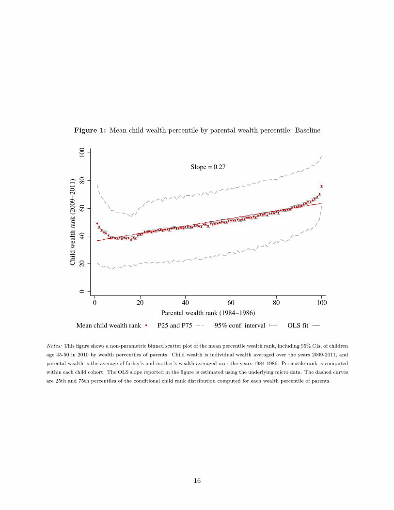
Figure 1: Mean child wealth percentile by parental wealth percentile: Baseline

Slope = 0.27

020

40

60

80

100

Chil

d w

ealt

h r

ank (

2009−

2011)

0 20 40 60 80 100

Parental wealth rank (1984−1986)

Mean child wealth rank P25 and P75 95% conf. interval OLS fit

Notes: This figure shows a non-parametric binned scatter plot of the mean percentile wealth rank, including 95% CIs, of childrenage 45-50 in 2010 by wealth percentiles of parents. Child wealth is individual wealth averaged over the years 2009-2011, andparental wealth is the average of father’s and mother’s wealth averaged over the years 1984-1986. Percentile rank is computedwithin each child cohort. The OLS slope reported in the figure is estimated using the underlying micro data. The dashed curvesare 25th and 75th percentiles of the conditional child rank distribution computed for each wealth percentile of parents.

16

Figure 2: Mean child wealth percentile by parental wealth percentile: Sensitivity analysis

(a) Without self-employed

Slope = 0.26

02

04

06

08

01

00

Ch

ild

wea

lth

ran

k (

20

09

−2

01

1)

0 20 40 60 80 100



(b) Parental wealth measured 2009–2011

Slope = 0.28

02

04

06

08

01

00

Ch

ild

wea

lth

ran

k (

20

09

−2

01

1)

0 20 40 60 80 100



Notes: Panel A is similar to figure 1 but made for the sub-sample where neither parent nor child are registered as self-employedat the period of measurement. Panel B is similar to figure 1 but parental wealth is measured in 2009–2011, like child wealth,instead of in 1984-1986.

percentile 99 to 100 in the parental wealth distribution. Thus, for the top 1% of parents, less than

25% of their children have a rank below 60. Moreover, the graph shows that 25% of the children

have a rank equal to 98% or higher.

Figure 2, panel A is similar to the above baseline figure but is made for a sub-sample where

neither parents nor children are self-employed when observing their wealth. The graph is very

similar to Figure 1, and with identical overall rank correlation. The main difference is that the dip

down at the bottom of the parental distribution is much less pronounced. In panel B, we redo the

baseline graph but based on parental wealth measured in 2009–2011 instead of in 1984–1986. This

move 25 years forward in the time of measurement of parents has nearly no impact on the graph

with the exception of nearly removing the dip down at the bottom of the parental distribution,

which increases the overall correlation coefficient a little.

In Figure 3, we repeat the baseline analysis for income. In the income concept, we include

earnings and self-employment income but not capital income, as we want to focus only on the

return to human capital. We find an almost completely linear relationship between ranks of children

and parents with a rank correlation of 0.2, which should be compared to the 0.27 for wealth.

Hence, wealth displays less mobility than income. This is in particular the case at the top of the

distributions where child wealth is much more strongly related to parental wealth than is the case

for income.

17

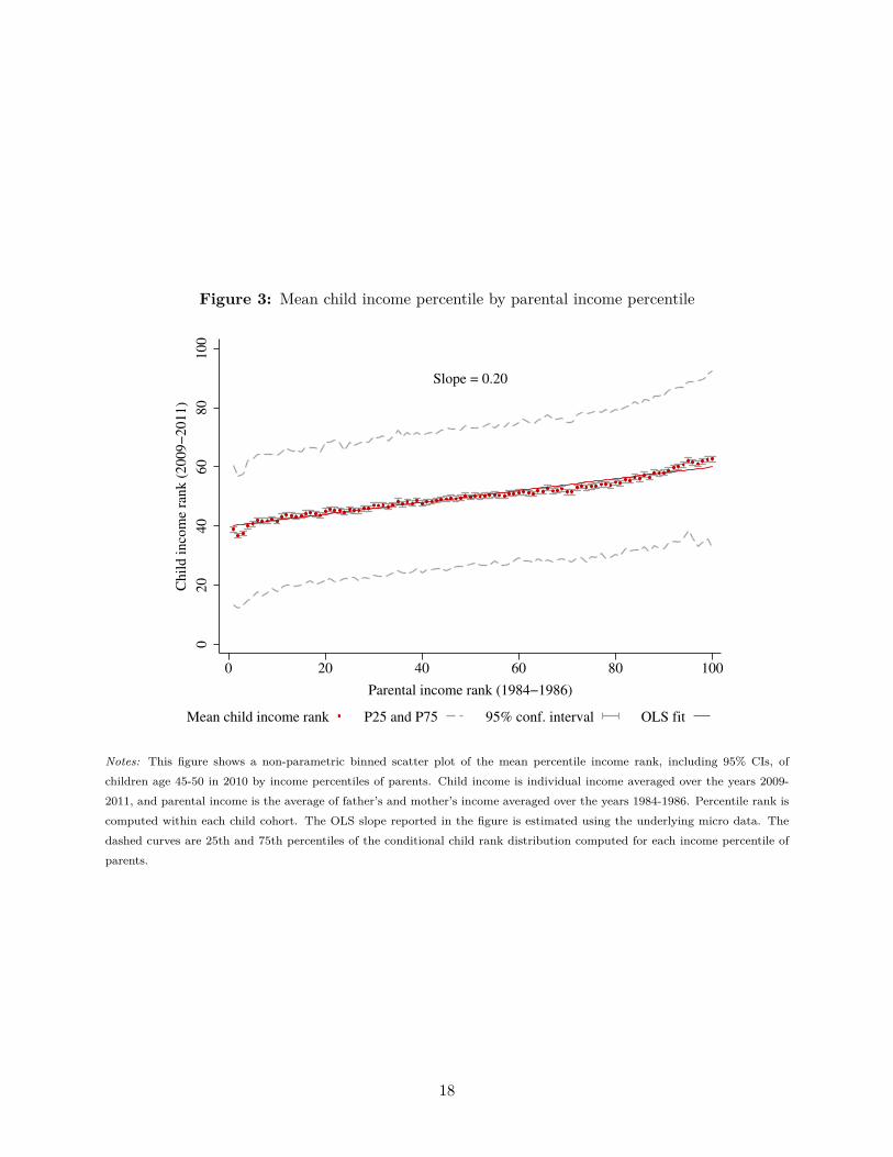
Figure 3: Mean child income percentile by parental income percentile

Slope = 0.20

020

40

60

80

100

Chil

d i

nco

me

rank (

2009−

2011)

0 20 40 60 80 100

Parental income rank (1984−1986)

Mean child income rank P25 and P75 95% conf. interval OLS fit

Notes: This figure shows a non-parametric binned scatter plot of the mean percentile income rank, including 95% CIs, ofchildren age 45-50 in 2010 by income percentiles of parents. Child income is individual income averaged over the years 2009-2011, and parental income is the average of father’s and mother’s income averaged over the years 1984-1986. Percentile rank iscomputed within each child cohort. The OLS slope reported in the figure is estimated using the underlying micro data. Thedashed curves are 25th and 75th percentiles of the conditional child rank distribution computed for each income percentile ofparents.

18

It is useful to have a single measure of the overall degree of wealth mobility. Our preferred

measure is the rank correlation coefficient. Because of the uniform distribution of the rank measure,

this may be obtained from a linear regression of child rank on the rank of parents, corresponding

to the slope of the OLS fitted line in Figure 1. The result of this regression, reported in panel A of

Table 2, is the baseline estimate of 0.27, which is very precisely estimated (standard deviation of

0.002) because of the large sample size. Thus, on average a one percentile increase in the position of

parents in the wealth distribution is associated with a 0.27 percentile increase in the average position

of children, in line with the conclusion above that the slope in Figure 1 is 1/4 almost everywhere

with the exception of at the tails of the parental distribution. Other studies of intergenerational

mobility, for example the study of wealth by Charles and Hurst (2003), analyze data where parents

are alive when wealth of children is measured—note that this creates an asymmetry as grandparents

may be dead when measuring the wealth of parents. Column 2 shows that the correlation coefficient

drops from 0.27 to 0.25, if restricting the sample in this way. In column 3, we repeat the baseline

analysis for the case where parental wealth is measured 12 years before the children, lying in

between the 25 year difference in the baseline analysis and the 0 year difference result in panel B

of Figure 2, making the result more comparable to Charles and Hurst (2003). In this case, the

correlation estimate increases somewhat. In column 4, we consider the impact of including age

dummy variables. Our percentile rank measure is already controlling for age as it is computed

within child cohorts but the estimate may still change when including age controls because of the

natural association between parental wealth and parental age at child birth. The table shows that

the rank correlation decreases slightly to 0.26. In column 5, we combine all three criteria studied

in columns 2-4, which bring the analysis closer to Charles and Hurst (2003). In this case, the rank

correlation is almost the same as in the baseline case.

For comparison, panel B of Table 2 also reports the elasticity of child wealth with respect

to parental wealth, corresponding to estimating an ordinary least squares regression after using

a natural logarithmic transformation of the data (for those with positive wealth). Studies on

intergenerational income mobility normally report the intergenerational elasticity, and this is also

done by Charles and Hurst (2003) in their study of intergenerational wealth mobility. In the

baseline case, we obtain a child-parents elasticity of 0.24, implying that children born to parents

with a wealth level that is 1 percent above the mean of the parental generation can expect to

obtain a wealth level that is 0.24 percent above the mean of the child generation. We obtain nearly

the same estimate in column 5, which may be compared to the result of 0.37 for the United States

19

reported by Charles and Hurst (2003). The lower estimate for Denmark is not surprising. Denmark

has a very homogeneous population and a high degree of redistribution, and comparative studies

find that Denmark has a high intergenerational mobility in earnings/income compared to the US

and many other countries (Björklund and Jäntti 2009; Chetty et al. 2014).

When applying the log transformation, we are throwing away all child-parents pairs where either

the child or the parents have zero or negative net wealth, which may generate selection problems.14

In panel C, we show the result when we instead apply the inverse hyperbolic sine transformation

w = log(W +√W 2 + 1), which behaves like the log transformation while allowing for negative

values. In this case, the elasticity estimates become considerably lower than the log transformation

estimate in the first columns but considerably higher in column 3.

4.2 Intergenerational correlation over the life cycle

In this section, we exploit the long panel dimension of our data to study the wealth formation over

the life cycle of the child starting at age 20 and going up to age 45. Compared to the previous

section, we limit the sample to the cohort born in 1965 who is 45 years old in 2010, and 20 years

old in 1985. As in the previous section, we measure parental wealth in mid-life in 1984-1986. We

also measure child wealth as a three-average starting with 1984-1986.

Figure 4 shows the correlation between the wealth of parents measured in mid-life, as in the

previous section, and wealth of the children measured at different points in the life cycle. For

comparison, the figure shows a similar graph for the correlation in income. The wealth correlation

is U-shaped. It starts at a high level of 0.35 and then declines until the mid-twenties at a level close

to 0.17 and then increases up to around 0.27 as in our baseline graph in Figure 1. The theory points

to two counteracting forces that determine the intergenerational correlation in wealth when the child

is young. The more prone parents are to give intervivo wealth transfers, the higher is the correlation.

On the other hand, the stronger the relationship between parental wealth and permanent income

of the child and the more prone children are to receive wealth transfers late in life, the higher is the

consumption level of the child when young, and the lower is the intergenerational wealth correlation.

Without any intervivo transfers received by the child when young, the intergenerational wealth14Most of the empirical literature analyzing intergenerational relationships have looked at economic outcomes

that do not attain negative values by definition, for example earnings. In this case, it is natural to apply the logtransformation, which has appealing properties. This is, however, not the case when analyzing net wealth, which maywell be negative, and where standard life cycle theory predicts negative values for young persons who have increasingearnings profiles. Another reason for observing negative wealth of households in our case, and also in C&H, is thatwe are unable to include pension wealth.

20

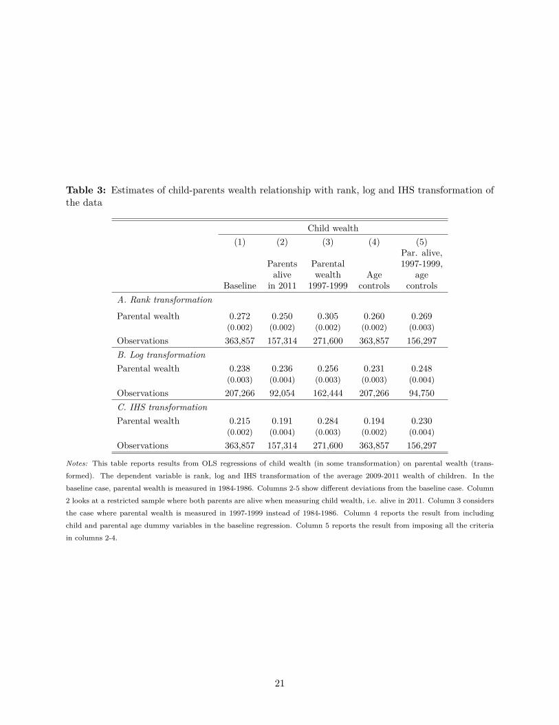
Table 3: Estimates of child-parents wealth relationship with rank, log and IHS transformation ofthe data

Child wealth(1) (2) (3) (4) (5)

Par. alive,Parents Parental 1997-1999,alive wealth Age age

Baseline in 2011 1997-1999 controls controlsA. Rank transformation

Parental wealth 0.272 0.250 0.305 0.260 0.269(0.002) (0.002) (0.002) (0.002) (0.003)

Observations 363,857 157,314 271,600 363,857 156,297B. Log transformationParental wealth 0.238 0.236 0.256 0.231 0.248

(0.003) (0.004) (0.003) (0.003) (0.004)Observations 207,266 92,054 162,444 207,266 94,750C. IHS transformationParental wealth 0.215 0.191 0.284 0.194 0.230

(0.002) (0.004) (0.003) (0.002) (0.004)Observations 363,857 157,314 271,600 363,857 156,297

Notes: This table reports results from OLS regressions of child wealth (in some transformation) on parental wealth (trans-formed). The dependent variable is rank, log and IHS transformation of the average 2009-2011 wealth of children. In thebaseline case, parental wealth is measured in 1984-1986. Columns 2-5 show different deviations from the baseline case. Column2 looks at a restricted sample where both parents are alive when measuring child wealth, i.e. alive in 2011. Column 3 considersthe case where parental wealth is measured in 1997-1999 instead of 1984-1986. Column 4 reports the result from includingchild and parental age dummy variables in the baseline regression. Column 5 reports the result from imposing all the criteriain columns 2-4.

21

correlation is negative. Thus, the high correlation in wealth at the time when the child moves

into adulthood is in the theory explained by a sufficiently high level of intervivo transfers. The

decline in the wealth correlation during the twenties is consistent with investments in human capital

and higher consumption levels of children with wealthy parents due to higher levels of economic

resources in the future. In mid-life these child have high incomes and build up wealth thereby

creating a higher correlation with parental wealth again. All in all, this pattern over the life cycle

is consistent with our theory of intergenerational wealth formation over the life-cycle with wealthy

parents leading to significant intervivo-transfers and human capital investments early in adulthood

and to high permanent incomes of children later in life (although the theory for simplicity only has

three periods of life).

Appendix B provides a repeated cross-section analysis showing that the U-shaped life-cycle

profile in wealth correlation exists over time and is not related to the particular cohorts studied

here.

The graph for the intergenerational correlation of income over the life cycle is very different from

the correlation of wealth. The correlation is lower at all ages and the correlation starts by being

negative, implying that high income parents have low-income children in the early twenties, and

then increases gradually as a function of child age. To get a better understanding of the connection

between the results for wealth and income, we divide the children into 10 groups depending on the

decile the parents belong to in the parental wealth distribution, and then plot the average wealth

and income percentile ranks of the children over the life-cycle. Figure 5 shows the results.

The graph for wealth shows that children systematically, with the exception of decile 1, at all

points in the life-cycle lie higher in the wealth distribution when the parents belong to a higher

wealth decile. The relationship with parental wealth is particular strong in the beginning of the

life-cycle where the groups of children lie in the range 35–70 depending on the position of the

parents. The variation becomes smaller until the mid-twenties and then increases again, thereby

mirroring the U-shaped pattern of the intergenerational wealth correlation in Figure 4. The graph

for income shows a negative—but very small—correlation between wealth of parents and income

of children in early adulthood. Over the life-cycle of the child the relationship between income of

the child and original wealth of the parents is reversed, and from the child turns thirty years old

and forward the relationship is stable and reveals a systematically higher permanent income level

of children having parents who were high up in the wealth distribution when the child was young.

In accordance, with the theory this is showing that the high intergenerational correlation in wealth

22

Figure 4: Intergenerational rank correlation in wealth and income over the life cycle of the child

Income

Wealth

−0.05

0.00

0.05

0.10

0.15

0.20

0.25

0.30

0.35

Ran

k c

orr

elat

ion

20 25 30 35 40 45Child age

Notes: The figure shows OLS estimates of the intergenerational rank correlation of wealth and income at each age of the childand 95% confidence intervals. Children are 45 years old in 2010 and 20 years old in 1985. Their wealth is measured as threeyear averages from 1984-1986 to 2009-2011. Parental wealth is the average of father’s and mother’s wealth averaged over theyears 1984-1986. Percentile ranks are computed within each child cohort.

when the child is young is not driven by a high income of children with wealthy parents—implying

that it has to be driven by intervivo transfers—and that children of wealthy parents have high

permanent incomes.

Note, finally, that when looking at the patterns of wealth and income in Figure 5 over the stable

life-cycle period from age 35 to 45 then parental wealth is a stronger predictor of the position of

the child in the wealth distribution, with children being in the percentile range 38-67 in panel A,

than in the income distribution, with children being in the percentile range 42-58 in panel B.

4.3 Role of bequests

In this section, we focus on the effects of bequests and the intergenerational correlation after death

of parents. We do not have direct information of bequest, as described in Section 3, but employ

an event study design where we look at child wealth before and after death of parents. Since

Danish laws permit a spouse to retain undivided possession of the estate, wealth is normally not

23

Figure 5: Development in child wealth and income by deciles of parental wealth distribution

40

50

60

70

Mea

n c

hil

d w

ealt

h r

ank

20 25 30 35 40 45Age

40

45

50

55

60

Mea

n c

hil

d i

nco

me

rank

20 25 30 35 40 45Age

Parental wealth decile: 1 2 3 4 5

6 7 8 9 10

Notes: The two graphs show average rank of children for wealth and income, respectively, at each age of the child by deciles ofparental wealth. Children are 45 years old in 2010 and 20 years old in 1985. Their wealth is measured as three year averagesfrom 1984-1986 to 2009-2011. Parental wealth is the average of father’s and mother’s wealth averaged over the years 1984-1986.Percentile ranks are computed within each child cohort.

24

transferred to the next generation before death of both parents. We therefore focus the analysis

on the sample of the children who have one living spouse in 2009, and divide the children into a

treatment group where the parent dies in 2010, and a control group where the parent does not

die in 2010. We continue to focus on the cohorts of children who are 45–50 years old in 2010 and

continue to measure wealth of parents in 1984-86.

Note that, for this analysis, we compute the percentile ranks for each individual separately

for the T-group and for the C-group. The reason is that we wish to measure the change in the

intergenerational rank correlation within the T-group, which should not be mixed up with the effect

that T-group children move up in the overall wealth distribution compared to C-group children

where parents die later.

The graphs in Figure 6 are identical to our baseline graph in Figure 1, but instead of looking at

the sample of children where parents are alive in 2010, we look separately at the T-group and the

C-group of the new sample before (2007-2009) and after (2011-2013) death of the parent in the T-

group. Panel A shows the result for the two groups before parental death. It reveals no systematic

differences between the two groups and the rank correlations are almost identical and only a little

higher than the 0.25 reported in Figure 1. In the period after parental death, panel B shows that

T-group observations lie mostly below the C-group observations in the lower part of the diagram

and mostly above in the upper part of the diagram, and the rank correlation increases to 0.37. The

rank correlation for the C-group is nearly unchanged and the difference-in-difference estimate of

the change in the rank correlation gives an increase of about 0.1 due to bequests, corresponding to

an increase of 35 percent.

If this measurement, we cannot be sure that grandparents died before measuring parental wealth

because we cannot observe grandparents of children this old. In Figure 7, we provide a sensitivity

analysis where we instead measure parental wealth in 2007-2009, where parents are around 68-

73 years old, making it unlike that any of the grandparents are alive. In this case, pre-bequest

correlations are 0.28 for both groups, and it is also 0.28 for the control group in the post-bequest

period, while the intergenerational correlation coefficient of the T-group increases to 0.40.

Thus, our estimates of the intergenerational correlation measured in mid-life after receiving

bequests are in the range 0.37-0.40. This level of intergenerational correlation is higher than any

of the estimates obtained earlier in the life cycle (see panel A of Figure 4).

25

Figure 6: Impact of bequests on intergenerational rank correlation

Slopes

Control group 0.28 (0.002)

Treatment group 0.29 (0.012)

020

40

60

80

100

Chil

d w

ealt

h r

ank (

2007−

2009)

0 20 40 60 80 100


(a) Before death of parent in T-group

Slopes



020

40

60

80

100

Chil

d w

ealt

h r

ank (

2011−

2013)

0 20 40 60 80 100


(b) After death of parent in T-group

Notes: The graphs are similar to Figure 1 but are made for different samples. The T-group is individuals who are age 45-50 in2010, with one parent alive in 2009 and no living parents in 2010. The C-group is individuals who are age 45-50 in 2010, withone parent who is alive in 2009 and 2010. Panel A shows the mean percentile wealth rank based on average wealth of the childin 2007-2009 and by wealth percentiles of parents based on average wealth in 1984-1986. Panel B is similar to panel A, but thechild rank is based on avearge wealth in 2011-2013. Percentile rank is computed within each child cohort. The OLS slopes, andtheir standard deviations in parentheses, reported in the figure are estimated using the underlying micro data.26

Figure 7: Impact of bequests on intergenerational rank correlation: Parental wealth measured in2007-2009

(a) Before death of parent in T-group

Slopes



020

40

60

80

100

Chil

d w

ealt

h r

ank (

2007−

2009)

0 20 40 60 80 100


(b) After death of parent in T-group

Slopes



020

40

60

80

100

Chil

d w

ealt

h r

ank (

2011−

2013)

0 20 40 60 80 100


Notes: The graphs are similar to those in Figure 6, but are based on parental wealth measured in 2007-2009 instead of 1984-1986.

27

4.4 From correlation of wealth to correlation of lifetime resources

In our theoretical discussion, we showed that the intergenerational correlation of lifetime resources

is equal to wealth correlation as long as both parents and children are measured at the same

stage of the life-cycle and the bias in formula (3) is addressed. Figure 1 presents the correlation

without addressing that bias. Our theoretical framework revealed that addressing the bias simply

requires controlling for permanent income of parents and children (equation 4). Table 4 shows

the corresponding results using the 45-50 year old cohort of children and their parents observed

at approximately the same age. In the first two columns, we contrast the estimates of wealth

and income correlation absent controls: the correlation of wealth is higher than the correlation

of permanent income (measured as three-year average), but none of them may be interpreted as

an estimate of the correlation of lifetime resources. These regressions correspond to equations (2)

and (3), respectively, both of which are subject to the omitted variable bias. In the following two

columns, we implement two variants of specification (4), controlling for parental and children income

rank parametrically and non-parametrically. The estimated coefficient on parental wealth drops

modestly to about 0.24. According to our theoretical framework, given that it relies on measurement

of wealth at the same stage of life-cycle of parents and children, this is an estimate of the correlation

in lifetime resources of parents and children. This estimate is significantly higher than our estimate

of the correlation of lifetime income equal to 0.20. In appendix C, we redo the analysis with

logarithmic and IHS transformations of the data, instead of the rank transformation. This gives

an intergenerational elasticity of lifetime resources equal to 0.18-0.19 and an intergenerational

elasticity of permanent income equal to 0.11-0.12, thus confirming the overall conclusion that the

intergenerational relationship is significantly stronger for lifetime resources than for permanent

income.

In appendix D, we show that controlling for permanent income has modest but stabilizing

impact on the correlation of wealth measured at any age (an analogue of Figure 4).

In Table 5, we redo the analysis of bequest with income controls. This implies that the post-

bequest estimate drops to 0.34. The large increase in the intergenerational wealth correlation

following death of parents raises the question of whether our same-stage-of-life-cycle pre-bequest

estimate of 0.24 does in fact measure the correlation of lifetime resources. Our theoretical framework

does predict that the correlation should increase on receipt of bequests (this simply corresponds to

a discrete jump in γt, which then equal one). Furthermore, it makes it clear that either wealth of

28

Table 4: Correlation of wealth and lifetime resources

(1) (2) (3) (4)Childwealth

Childincome

Childwealth

Childwealth

Parental wealth rank (1984-1986) 0.272∗∗∗ 0.240∗∗∗ 0.235∗∗∗

(0.002) (0.002) (0.002)

Parental income rank (1984-1986) 0.200∗∗∗ 0.004∗

(0.002) (0.002)

Child income rank (2009-2011) 0.191∗∗∗

(0.002)

Child and parent income percentile dummies XObservations 363,857 363,857 363,857 363,857Adj. R-squared 0.074 0.040 0.110 0.114

Standard errors in parentheses∗ p < 0.05, ∗∗ p < 0.01, ∗∗∗ p < 0.001

both parents and children should be observed before bequest or they both should be observed after

bequests. Unfortunately, limitations of our data do not allow for observing parents after bequests

and our best approximation is to use observations 25 years later when grandparents are almost

certain to have died but parents are much older. Hence, we do not have a clean estimate of the

correlation in lifetime resources based on after-bequest observations.

What we know is that the large effect of bequests on impact reveals that bequests are quan-

titatively important. In fact, bequests are on average about 1/3 of pre-bequest children’s wealth

(Boserup, Kopczuk and Kreiner, 2016). However, children’s wealth at ages 45-50 is only a fraction

of lifetime resources: it does not account for income yet to be received (both during the remaining

career and post-retirement) and it already nets out past consumption. Hence, while bequests have

a large impact on wealth at that point, they are a much smaller component of lifetime resources.

5 Concluding remarks

This paper uses Danish administrative records to measure intergenerational correlation of wealth

and propose an interpretation of the relationship to the correlation of lifetime resources. We show

that the population correlation of wealth is about 0.27 and exceeds the correlation of lifetime

income. This correlation evolves over the life-cycle in a way that reveals the importance of life-

cycle patterns of income, consumption and transfers. It is very high at the beginning of the

29

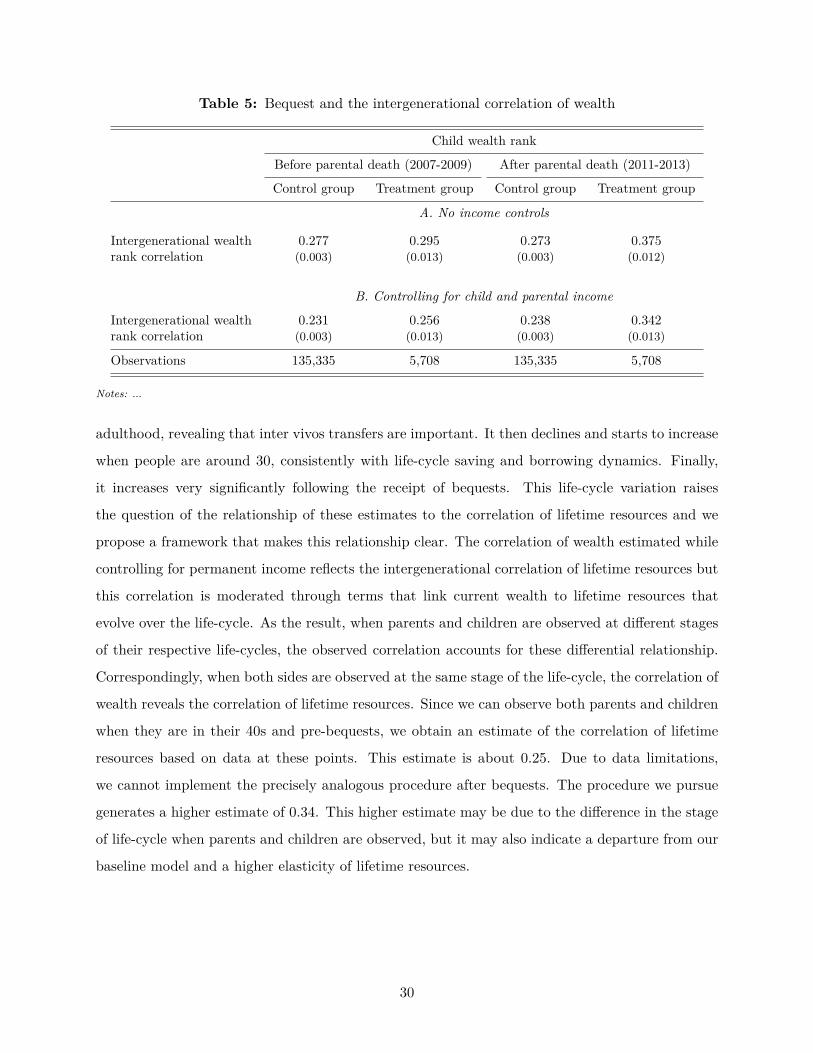
Table 5: Bequest and the intergenerational correlation of wealth

Child wealth rank

Before parental death (2007-2009) After parental death (2011-2013)

Control group Treatment group Control group Treatment group

A. No income controls

Intergenerational wealth 0.277 0.295 0.273 0.375rank correlation (0.003) (0.013) (0.003) (0.012)

B. Controlling for child and parental income

Intergenerational wealth 0.231 0.256 0.238 0.342rank correlation (0.003) (0.013) (0.003) (0.013)

Observations 135,335 5,708 135,335 5,708

Notes: ...

adulthood, revealing that inter vivos transfers are important. It then declines and starts to increase

when people are around 30, consistently with life-cycle saving and borrowing dynamics. Finally,

it increases very significantly following the receipt of bequests. This life-cycle variation raises

the question of the relationship of these estimates to the correlation of lifetime resources and we

propose a framework that makes this relationship clear. The correlation of wealth estimated while

controlling for permanent income reflects the intergenerational correlation of lifetime resources but

this correlation is moderated through terms that link current wealth to lifetime resources that

evolve over the life-cycle. As the result, when parents and children are observed at different stages

of their respective life-cycles, the observed correlation accounts for these differential relationship.

Correspondingly, when both sides are observed at the same stage of the life-cycle, the correlation of

wealth reveals the correlation of lifetime resources. Since we can observe both parents and children

when they are in their 40s and pre-bequests, we obtain an estimate of the correlation of lifetime

resources based on data at these points. This estimate is about 0.25. Due to data limitations,

we cannot implement the precisely analogous procedure after bequests. The procedure we pursue

generates a higher estimate of 0.34. This higher estimate may be due to the difference in the stage

of life-cycle when parents and children are observed, but it may also indicate a departure from our

baseline model and a higher elasticity of lifetime resources.

30

ReferencesBecker, Gary, and Nigel Tomes. 1979. “An Equilibrium Theory of the Distribution of Incomeand Intergenerational Mobility.” Journal of Political Economy, 87.

Becker, Gary, and Nigel Tomes. 1986. “Human Capital and the Rise and Fall of Families.”Journal of Labor Economics, 4(1–39).

Björklund, Anders, and Markus Jäntti. 2009. “Oxford Handbook of Economic Inequality.” ,ed. B. Nolan Salverda W. and T. Smeeding, Chapter Intergenerational Income Mobility and theRole of Family Background, 491–521. Oxford University Press.

Black, Sandra, and Paul J. Devereux. 2011. “Handbook of Labor Economics.” , ed. O. Ashen-felter and D. Card Vol. IVb, Chapter Recent Developments in Intergenerational Mobility, 1487–1541. North-Holland, Amsterdam.

Boserup, Simon Halphen, Wojciech Kopczuk, and Claus Thustrup Kreiner. 2016. “TheRole of Bequests in Shaping Wealth Inequality: Evidence from Danish Wealth Records.” Ameri-can Economic Review Papers and Proceedings. Forthcoming.

Charles, Kerwin K., and Erik Hurst. 2003. “The Correlation of Wealth across Generations.”Journal of Political Economy, 111: 1155–1182.

Chetty, Raj, Nathan Hendren, Patrick Kline, and Emmanuel Saez. 2014. “Where isthe Land of Opportunity? The Geography of Intergenerational Mobility in the United States.”Quarterly Journal of Economics, 129: 1553–1623.

Clark, Gregory, and Neil Cummins. 2015. “Intergenerational Wealth Mobility in England,1858–2012. Surnames and Social Mobility.” Economic Journal, 125: 61–85.

European Commission. 2012. “Alert mechanism report.”

Haider, Steven, and Gary Solon. 2006. “Life-Cycle Variation in the Association between Cur-rent and Lifetime Earnings.” American Economic Review, 96: 1308–1320.

International Monetary Fund. 2012. “World Economic Outlook (WEO): Growth Resuming,Dangers Remain.”

Kleven, Henrik J., Martin B. Knudsen, Claus T. Kreiner, Søren Pedersen, and Em-manuel Saez. 2011. “Unwilling or Unable to Cheat? Evidence from a Tax Audit Experimentin Denmark.” Econometrica, 79: 651–692.

Menchik, Paul. 1979. “Inter-generational Transmission of Inequality: An Empirical Study ofWealth Mobility.” Economica, 46: 349–362.

Solon, Gary. 1992. “Intergenerational Income Mobility in the United States.” American E, 82: 393–408.

Solon, Gary. 1999. “Handbook of Labor Economics.” , ed. O. Ashenfelter and D. Card Vol. III,Chapter Intergenerational mobility in the labor market, 1761–1800. North-Holland, Amsterdam.

Stiglitz, Joseph E. 1969. “Distribution of Income and Wealth Among Individuals.” Econometrica,37: 382–397.

31

Wahl, Jenny. 2003. “From Riches to Riches: Intergenerational Transfers and the Evidence fromEstate Tax Returns.” Social Science Quarterly, 84: 278–296.

32

A Impact of data break in year 1996The graph below shows that the data break in 1996 is not important. Wealth definitions overlap in1995-1996 and we obtain basically the same diagram and intergenerational rank correlation withboth definitions.

Figure A.1: Influence of change in wealth definition on intergenerational rank correlation0

20

40

60

80

100

Chil

d w

ealt

h r

ank (

2009−

2011)

0 20 40 60 80 100


Old definition (slope = 0.30)

New definition (slope = 0.30)

Notes: The wealth measures overlap in 1995 and 1996. The figure shows our baseline rank diagram when parental wealth ismeasured in 1995-1996 using the two different definitions of wealth.

B Robustness of U-shaped life cycle profile over time and acrosscohorts

In this graph, we measure children and parents at the same time (which we have to do becauseof data limitations), while in the others graphs we measure wealth of parents in 1984-1986. Thegraphs shows the correlation in wealth between children who are 18-25 years and their parents inthe different years, using information from different cohorts over time in a repeated cross-sectionanalysis. The graph shows that the correlation has increased somewhat over time. This could inprinciple be because of improvements in data quality. On the other hand, the large data break in1996 does not seem to have any important effect on the results An important conclusion from thegraph is in the vertical dimention showing that the youngest group has the highest intergenerationalcorrelation, then it drops down at the bottom for the next age group and then climbs somewhatup again. This mirrors the U-shaped profile in Figure 4.

33

Figure B.2: Intergenerational wealth correlation over time: repeated cross-section

0.00

0.05

0.10

0.15

0.20

0.25

0.30

0.35

0.40

Inte

rgen

erat

ional

ran

k c

orr

elat

ion

1985 1990 1995 2000 2005 2010Year

Age groups: 18−25 26−30 31−35 36−40 41−45 46−51

Notes: In this diagram child wealth and parental wealth is mesured in the same years using three-year averages (the observationfor 1985 is computed using 1984-1986 data).

C Estimation of the intergenerational elasticity of lifetime re-sources

Tables C.1 and C.2 show the results, when we redo the analysis with logarithmic and IHS transfor-mations of the data, instead of the rank transformation. This gives an intergenerational elasticityof lifetime resources equal to 0.18-0.19 and an intergenerational elasticity of permanent incomeequal to 0.11-0.12, thus confirming the overall conclusion that the intergenerational relationship issignificantly stronger for lifetime resources than for permanent income.

D Impact of controlling for permanent income in Figure 4

The Figure below shows the impact of controlling for permanent income at any age — the imple-mentation of regression specification (4) not just at the same stage of life-cycle as in Section 4.4but rather varying age of a child as in Figure 4. The bias that permanent income control correctsfor is due to the presence of the −νs

t ug−1 term in equation (3) and closer inspection of it revealsthat the sign of νs

t may vary over the life-cycle. The figure shows that indeed correction of the biasincreases the estimate of wealth correlation in late 20s and reduces it in the 30s and 40s so that theunderlying direction of the bias changes sign. The revealed pattern of correlation over the life-cycletraces the value (αe + αQ)bs

t . Given that the estimated bias-corrected correlation is approximatelyconstant when children are in their 30s and 40s, this suggests that bs

t is about constant over this

34

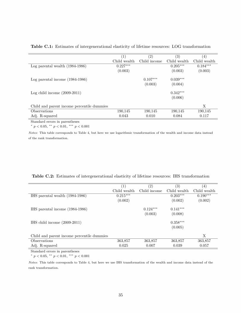
Table C.1: Estimates of intergenerational elasticity of lifetime resources: LOG transformation

(1) (2) (3) (4)Child wealth Child income Child wealth Child wealth

Log parental wealth (1984-1986) 0.227∗∗∗ 0.205∗∗∗ 0.184∗∗∗

(0.003) (0.003) (0.003)

Log parental income (1984-1986) 0.107∗∗∗ 0.039∗∗∗

(0.003) (0.004)

Log child income (2009-2011) 0.342∗∗∗

(0.006)

Child and parent income percentile dummies XObservations 190,145 190,145 190,145 190,145Adj. R-squared 0.043 0.010 0.084 0.117Standard errors in parentheses∗ p < 0.05, ∗∗ p < 0.01, ∗∗∗ p < 0.001

Notes: This table corresponds to Table 4, but here we use logarithmic transformation of the wealth and income data insteadof the rank transformation.

Table C.2: Estimates of intergenerational elasticity of lifetime resources: IHS transformation

(1) (2) (3) (4)Child wealth Child income Child wealth Child wealth

IHS parental wealth (1984-1986) 0.215∗∗∗ 0.203∗∗∗ 0.190∗∗∗

(0.002) (0.002) (0.002)

IHS parental income (1984-1986) 0.124∗∗∗ 0.141∗∗∗

(0.003) (0.008)

IHS child income (2009-2011) 0.358∗∗∗

(0.005)

Child and parent income percentile dummies XObservations 363,857 363,857 363,857 363,857Adj. R-squared 0.025 0.007 0.039 0.057Standard errors in parentheses∗ p < 0.05, ∗∗ p < 0.01, ∗∗∗ p < 0.001

Notes: This table corresponds to Table 4, but here we use IHS transformation of the wealth and income data instead of therank transformation.

35

range. Furthermore, given that this range includes t = s (parents are measured when they arein their 40s) at which point bs

t = 1, this suggests the estimate of the lifetime correlation is notvery sensitive to the precise time when parental and children’s wealth is observed, as long as it ismeasured in 30s or 40s.

Figure D.3: Rank correlation in wealth over the life cycle of the child: With and without incomecontrols

Controlling for permanent income

No controls

0.00

0.05

0.10

0.15

0.20

0.25

0.30

0.35

Wea

lth r

ank c

orr

elat

ion

20 25 30 35 40 45Child age

Notes: This curve with income controls corresponds to the curve in Figure 4. The curve with income controls includes averageincome of the child in 2009-2011 and of the parents in 1984-1986 in the specification when estimating the intergenerationalwealth correlation at each age of the child.

36

Stability and persistence of intergenerational wealth ...wk2110/bin/WealthAcrossGen.pdf ·...

Documents

Transcript of Stability and persistence of intergenerational wealth ...wk2110/bin/WealthAcrossGen.pdf ·...