Wealth Inequality: A Survey

by

Frank A. CowellSTICERD

London School of EconomicsHoughton Street

London, WC2A 2AE, UKf.cowell@lse.ac.uk

and

Philippe Van KermLuxembourg Institute of Socio-Economic Research

3, avenue de la FonteL-4364 Esch-sur-Alzette Luxembourg

philippe.vankerm@liser.lu

April 2015

We thank Xuezhu Shi and Julia Philipp for excellent research assistance. Thispaper uses data from the Eurosystem Household Finance and Consumption Surveydistributed by the European Central Bank. The survey was initiated when VanKerm visited the London School of Economics with the support of the Luxem-bourg Fonds National de la Recherche (INTER/Mobility/13/5456106).

1 IntroductionThe distribution of wealth lies at the heart of the broad research field of economicinequality. It is a topic that has recently gained considerable attention in viewof the widespread phenomenon of increasing wealth inequality and given thegrowing availability of suitable data for analysing wealth inequality.

A survey of wealth inequality properly deserves a good-sized book ratherthan a modest-sized survey article, so we have necessarily been selective. Herewe concentrate on key aspects of the following problems:

The nature of wealth.

What is the appropriate definition of wealth? Is there a single “right” conceptof wealth that should be used for empirical analysis?

Measurement issues.

How does the measurement of the inequality of wealth differ from that of incomeor earnings?

Empirical implementation.

Where do wealth data come from? What are the appropriate procedures foranalysing wealth data and drawing inferences about changes in inequality?

So, in contrast with some other surveys,1 we have deliberately kept the rangeof topics narrow and have focused our attention more on the measurement ap-paratus – inequality indicators, parametric functional forms, inference – and inparticular point out what is different from the tools and procedures appropriateto income inequality measurement. We only briefly discuss theoretical models ofwealth accumulation and do not attempt to summarize the empirical evidenceon wealth inequality internationally but instead provide some fresh empiricalevidence drawn from recently collected survey data in Europe. We focus on the“direct” issue of wealth inequality, rather than discussing aspects of inequalitythat are indirectly related to wealth holdings2 or related issues such as poverty.3

Throughout the paper, we illustrate a number of concepts and methodsdiscussed in this survey using data from the Eurosystem Household Financeand Consumption Survey (HFCS) initiated and coordinated by the EuropeanCentral Bank (HFCS 2014). We use the first wave of HFCS which collectedhousehold-level data on household finances and consumption in late 2010 or

1Detailed surveys of the literature on wealth inequality are available in Jenkins (1990),Davies and Shorrocks (2000) or Davies (2009).

2For example we exclude discussion of debt constraints and incomplete asset markets (Cor-doba 2008) or the role of capital gains from asset holdings on the distribution of income(Alvaredo et al. 2013, Roine and Waldenström 2012).

3On the important related issue of asset-based poverty see Azpitarte (2011), Fisher andWeber (2004), Brandolini et al. (2010), Carter and Barrett (2006), Carney and Gale (2001),Caner and Wolff (2004), Haveman and Wolff (2004), Rank and Hirschl (2010).

1

early 2011 in 15 Eurozone countries. The HFCS provides comparable dataacross eurosystem countries using coordinated definitions of core target vari-ables, harmonized questionnaire templates and survey design and processing.The HFCS was modelled on the US Survey of Consumer Finances, the “goldstandard” of household wealth surveys. See European Central Bank (2013) fordetails.

The paper is organised as follows. We begin with measurement issues: sec-tion 2 examines the basic issues of the measurement of wealth and section 3focuses on the way in which wealth-inequality measurement differs from in-equality measurement in other contexts. Section 4 discusses issues relating toparametric and non-parametric representations of wealth distributions, section5 discusses some of the key features of wealth distributions that require specialcare when making inequality comparisons. Section 6 deals with empirical issuesfrom the way the underlying data are obtained through to some of the morerecondite issues concerning estimation and inference.

2 Measuring wealthThe right place to start is the meaning of wealth. It has variously been seenas a simple stock of assets, a measure of command over resources, or a keycomponent of economic power (Atkinson 1975, p. 37; OECD 2013; Vickrey1947, p. 340).

A brief reflection on one’s own circumstances will probably be enough todemonstrate that wealth is not a homogeneous entity and a moment’s furtherreflection suggests that more than one concept of wealth may be relevant for thepurposes of inequality comparisons. The nature of wealth inequality is clearlygoing to depend on the definition that is adopted.

Wealth could in principle be taken to refer to one specific type of asset orgroup of assets. However, for most purposes the standard wealth concept thatis considered relevant for empirical analysis is current net worth which can bethought of as the following simple expression:

w =m∑j=1

πjAj −D (1)

where Aj ≥ 0 is the amount held of asset type j, πj is its price and D representsthe call on those assets represented by debt:4 the key notion of “net wealth”or “net worth” is the difference between assets and debts. The expression (1)reveals three things that ought to be taken into account:

• The range of asset types to be included; depending on institutional ar-rangements in particular countries some individual assets, such as housingand pensions, may need to be treated with special care.5

4Clearly one may also usefully break down the debt into different components.5For example although housing is usually very important for many households as a means

2

• the valuation applied to the assets, which may have a huge impact onwealth inequality. Is the market price being used for each asset j, or is itrather some type of imputed price?6

• the possibility that the expression (1) may be negative for some householdsat a given moment.

Furthermore in practice we often want to focus on household wealth which isclearly the sum of all assets minus debts for all the household members. We mayalso wish to distinguish between real and financial assets: real assets include thevalue of household’s main residence, real estate property other than the mainresidence, self-employment businesses, vehicles, jewelry, etc.; financial assetsinclude deposits on current or savings accounts, voluntary private pensions andlife insurance, mutual funds, bonds, shares, and other financial assets. Debtsinclude home-secured debts (principal residence mortgage primarily), vehicleloans, educational loans, lines of credit and credit card balance, and any otherfinancial loans and informal debts. Typically one finds that assets are primarilycomposed of real rather than financial assets. In the Eurozone countries, realassets represent 85% of total gross assets (European Central Bank 2013). Andthe household main residence is typically the lion’s share of real assets (61% onaverage in the Eurozone). Financial assets are mostly composed of deposits andsavings accounts. Debts largely consist of mortgage debt.

Clearly wealth contributes to individual well-being over and above any in-come flows that may arise from the wealth-holding, including economic andfinancial security and some form of economic power. Accounting for such ben-efits is in itself an interesting exercise,7 but for now it is sufficient to note thattranslating wealth into an equivalent income stream, or vice versa, is an exercisethat may miss some of the personally beneficial aspects of wealth holding andthat the study of wealth inequality is an exercise that merits separate investi-gation and study, distinct from the study of income inequality.

of asset accumulation (Denton 2001, Silos 2007) it is sometimes difficult to disentangle housingwealth and housing debt – see the case of Sweden discussed in (Cowell et al. 2012). Sometimesit is not clear which forms of pension wealth should be included in wealth computations, butthe inclusion or exclusion of this form of wealth can make a huge difference to measured wealthinequality. In the UK the HMRC this used to be dramatically illustrated by its series C, seriesD and series E definitions of wealth inequality (Hills et al. 2013 page 32): augmenting networth with private pension wealth typically reduced inequality unambiguously and furtheraugmenting it with the wealth attributable to the state-provided retirement pension reducedinequality still more. However, those data largely applied to an era of traditional defined-benefit (DB) pensions; the switch to defined-contribution (DC) pensions that has occurredin many countries in recent years is unlikely to have been inequality-neutral, because DCpensions are unequal compared to DB pensions and are likely to be positively correlated withnet worth. As a result the DB-to-DC switch is likely to have increased inequality when networth is augmented by pension wealth (Wolff 2015).

6For an interesting practical analysis of how a sharp changes in asset prices affect thewealth distribution see Wolff (2012). For a careful analysis of the dramatic effect of houseprices on wealth inequality in the UK see Bastagli and Hills (2013).

7Appropriately accounting for wealth in this way substantially changes the structure of thedistribution of economic well-being (Wolff and Zacharias 2009).

3

The precise definition is not a matter of purely technical interest. It isoften the case that practical applications that appear conceptually straightfor-ward prove to be considerably more complicated because of the ambiguity ofthe wealth concept or the different ways in which supposedly the same wealthconcept is interpreted in different countries or at different times.

To fix ideas, Table 1 describes the size and composition of net worth ascalculated in 15 countries from the Eurosystem Household Finance and Con-sumption Survey. In each country a (small) fraction of households – between1 and 12 percent – report negative or zero net worth and mean net worth isgenerally large and positive. Mean net worth is also much higher than mediannet worth: net worth distributions are indeed strongly left-skewed. Inspectionof the components of net worth illustrate how important is the value of themain residence in the net worth with between 44 percent (in Germany) and90 percent (in Slovakia) of household having some wealth from this particularasset. Between 25 percent (in Italy) and 65 percent (in Cyprus) hold somedebt. While the HFCS aims to collect fully comprehensive and detailed infor-mation on a wide array of asset sources (our estimates are aggregates of finercomponent details available in the source data), cross-country data collectionsremain inevitably imperfect. Some components were not fully systematicallycollected in all countries – Finland for example does not record a range of as-set sources – while some differences in underlying survey design may lead tonational peculiarities; see Tiefensee and Grabka (2014) for a detailed review ofdata quality and cross-country comparability of HFCS data. Note finally thatone potentially crucial wealth component for cross-country comparisons that isnot available from the HFCS are public pension entitlements.8 It remains thecase that the HFCS is probably the best quality survey data source on wealthavailable to date for cross-national comparisons.

3 Inequality measurementA survey on the inequality of anything almost always raises measurement issues.Some conceptual and measurement issues make measurement of inequality ofwealth somewhat more challenging than analysis of income or consumption –these include the presence of a substantial fraction of negative net worth in mostsample data on wealth, and the skewness and fat tails of the wealth distributionsresulting in sparse, extreme data in typical samples of data on wealth. Thesefeatures make some traditional measures of relative inequality inadequate, inparticular because of negative net worth (Jenkins and Jäntti 2005). We illus-trate in this section how these can be taken into account in our measurementapparatus. The presence of negative net worth also requires the design of dif-ferent parametric models from those typically used for income distribution; weaddress this in section 4. Finally, extreme data affect the performance of stan-dard statistical inference apparatus (for point estimation, sampling variance

8Including public pension entitlements would normally reduce wealth inequality – see note5.

4

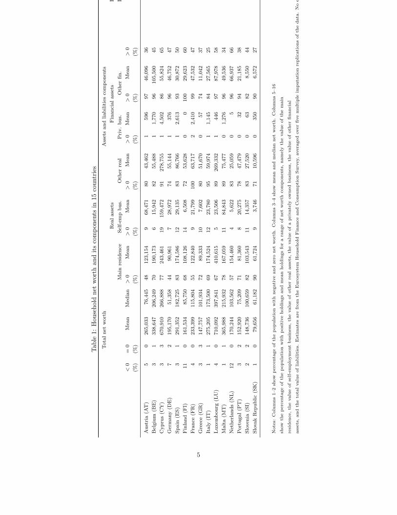
Table1:

Hou

seho

ldne

tworth

andits

compo

nentsin

15coun

tries

Totaln

etworth

Assetsan

dlia

bilitiescompo

nents

Reala

ssets

Finan

cial

assets

Debts

Mainresidence

Self-em

pbu

s.Other

real

Priv.

bus.

Other

fin.

Debts

<0

=0

Mean

Median

>0

Mean

>0

Mean

>0

Mean

>0

Mean

>0

Mean

>0

Mean

(%)

(%)

(%)

(%)

(%)

(%)

(%)

(%)

Austria

(AT)

50

265,03

376

,445

48123,154

968,471

8043,462

1596

9746,096

3616,746

Belgium

(BE)

31

338,647

206,249

70190,173

615,942

8255,488

11,770

96105,500

4530,226

Cyp

rus(C

Y)

33

670,91

026

6,888

77243,461

19159,472

91278,755

14,502

8655,824

6571,104

German

y(D

E)

72

195,17

051,358

4490,961

728,972

7455,144

1376

9646,752

4727,035

Spain(E

S)3

129

1,352

182,725

83174,586

1229,135

8386,766

12,613

9330,872

5032,621

Finland

(FI)

110

161,53

485,750

68108,126

146,508

7253,628

00

100

29,623

6036,351

Fran

ce(F

R)

40

233,39

911

5,804

55122,840

921,799

100

63,717

22,410

9947,532

4724,898

Greece(G

R)

33

147,75

710

1,934

7289,333

107,602

8051,670

057

7411,042

3711,948

Italy(IT)

11

275,20

517

3,500

69174,524

1223,780

9559,974

11,145

8427,565

2511,784

Luxembo

urg(L

U)

40

710,09

239

7,841

67410,615

523,506

89269,332

1446

9787,978

5881,785

Malta

(MT)

11

365,98

821

5,932

78167,059

1184,843

8975,477

01,276

9649,536

3412,203

Netherlan

ds(N

L)12

017

0,24

410

3,562

57154,460

45,622

8325,059

05

9666,937

6681,840

Portuga

l(PT)

32

152,92

075,209

7181,360

820,275

7847,479

032

9421,185

3817,410

Slovenia

(SI)

22

148,736

100,659

82103,543

1114,357

8327,520

063

828,550

445,297

Slovak

Repub

lic(SK)

10

79,656

61,182

9061,724

93,746

7110,596

0350

906,572

273,332

Notes:Colum

ns1–2show

percentage

ofthepo

pulation

withne

gative

andzero

networth.Colum

ns3–4show

meanan

dmed

ianne

tworth.Colum

ns5–16

show

thepe

rcentage

ofthepo

pulation

withpo

sitive

holdings

andmeanho

ldings

forarang

eof

networth

compo

nents,

namelythevalueof

themain

reside

nce,

thevalueof

self-em

ploy

mentbu

sine

ss,thevalueof

othe

rreal

assets,thevalueof

aprivatelyow

nedbu

sine

ss,thevalueof

othe

rfin

ancial

assets,an

dthetotalvalueof

liabilities.

Estim

ates

arefrom

theEurosystem

Hou

seho

ldFinan

cean

dCon

sumptionSu

rvey,averaged

over

fivemultipleim

putation

replications

oftheda

ta.Noequivalenc

escales

areap

plied.

5

estimation and testing) and call for robust estimation techniques to keep theimpact of extreme data under control (Cowell and Victoria-Feser 1996, Cowelland Flachaire 2015). We address these additional issues in section 6.3.

3.1 PrinciplesIn principle the measurement of inequality of wealth should be just like themeasurement of inequality of income – almost. There will be differences betweenthe two areas of application because some of the issues that arose in section 2affect what one can logically do within the context of wealth inequality.

The equalisand

In the case of income inequality it is usually appropriate to assume that theequalisand (income, earnings) is something that is intrinsically non-negative.Of course researchers with practical experience will quickly point out excep-tions to this (for example, where an individual’s business losses are sufficientlygreat to make annual income negative) but, in the main, they are just that,exceptions. However, the non-negativity assumption just will not do in the caseof wealth. If we want to examine the inequality of net worth – which is formany researchers, the theoretically ideal wealth concept – then we have to ac-cept that in many cases a substantial proportion of the population will havenegative current wealth.

In the case of income inequality there are good arguments for using equiv-alised income as an appropriate indicator of current individual welfare withina household. Converting total household income y of a family consisting of nAadults and nC children into the “single-adult equivalent income” of each house-hold member is considered uncontroversial and indeed their is a broad consensusas to the precise equivalence scale to use: many studies use either the square-root scale (dividing y by

√nA + nC) or the modified OECD scale (dividing y by

1+0.5(nA−1)+0.3nC). The application of such scales is intended to account foreconomies of scale in household spending and the lower needs of children whenevaluating the living standard attained with a given income level and householdsize. By contrast, application of equivalence scales to household wealth datais more controversial (Bover 2010, Jäntti et al. 2013, OECD 2013, Sierminskaand Smeeding 2005). A key issue is that if wealth is interpreted as the value ofpotential future consumption (say after retirement), it is not current householdcomposition that should matter, but future composition. In case wealth is as-sumed to be consumed after retirement, one would probably not want to accountfor the presence of children in the household (but bequest intentions and futureinter-vivos transfers make this decision less than obvious). Of course, if insteadone is willing to interpret wealth as the ability to finance current consumption,arguments for applying equivalence scales are strong. Along an entirely differ-ent line of reasoning, if one does not interpret wealth as potential consumptionbut instead interprets wealth as an indication of status or power, there is littlereason to adjust wealth for household size at all. Practice therefore varies in

6

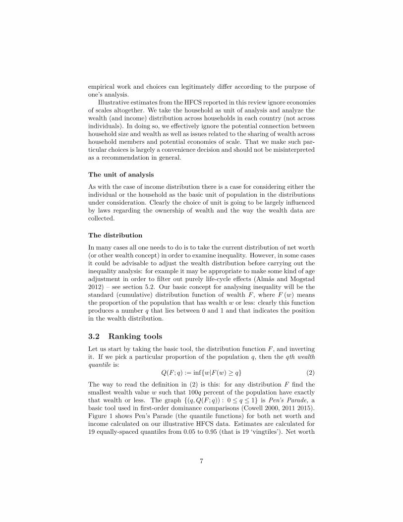
empirical work and choices can legitimately differ according to the purpose ofone’s analysis.

Illustrative estimates from the HFCS reported in this review ignore economiesof scales altogether. We take the household as unit of analysis and analyze thewealth (and income) distribution across households in each country (not acrossindividuals). In doing so, we effectively ignore the potential connection betweenhousehold size and wealth as well as issues related to the sharing of wealth acrosshousehold members and potential economies of scale. That we make such par-ticular choices is largely a convenience decision and should not be misinterpretedas a recommendation in general.

The unit of analysis

As with the case of income distribution there is a case for considering either theindividual or the household as the basic unit of population in the distributionsunder consideration. Clearly the choice of unit is going to be largely influencedby laws regarding the ownership of wealth and the way the wealth data arecollected.

The distribution

In many cases all one needs to do is to take the current distribution of net worth(or other wealth concept) in order to examine inequality. However, in some casesit could be advisable to adjust the wealth distribution before carrying out theinequality analysis: for example it may be appropriate to make some kind of ageadjustment in order to filter out purely life-cycle effects (Almås and Mogstad2012) – see section 5.2. Our basic concept for analysing inequality will be thestandard (cumulative) distribution function of wealth F , where F (w) meansthe proportion of the population that has wealth w or less: clearly this functionproduces a number q that lies between 0 and 1 and that indicates the positionin the wealth distribution.

3.2 Ranking toolsLet us start by taking the basic tool, the distribution function F , and invertingit. If we pick a particular proportion of the population q, then the qth wealthquantile is:

Q(F ; q) := inf{w|F (w) ≥ q} (2)

The way to read the definition in (2) is this: for any distribution F find thesmallest wealth value w such that 100q percent of the population have exactlythat wealth or less. The graph {(q,Q(F ; q)) : 0 ≤ q ≤ 1} is Pen’s Parade, abasic tool used in first-order dominance comparisons (Cowell 2000, 2011 2015).Figure 1 shows Pen’s Parade (the quantile functions) for both net worth andincome calculated on our illustrative HFCS data. Estimates are calculated for19 equally-spaced quantiles from 0.05 to 0.95 (that is 19 ‘vingtiles’). Net worth

7

quantiles exhibit much bigger disparities than income: they are both higherthan income quantiles at the top and flatter in most of the quantile range.

We can build on the concept defined in (2) to give us some other useful tools.The qth wealth cumulation is defined as:

C(F ; q) :=ˆ wq

w

w dF (w) (3)

where wq = Q(F ; q) and w is the lower bound of the support of F .9 An impor-tant special case of this is found when wq = w, the upper bound of the supportof F . The mean of the distribution F is defined as

µ (F ) :=ˆwdF (w) (4)

and clearly equals C (F, 1). The graph {(q, C(F ; q)) : 0 ≤ q ≤ 1} is the Gener-alised Lorenz curve which plots the (normalised) cumulations of wealth againstproportions of the population. It is a basic tool used in second-order dominancecomparisons (Shorrocks 1983). An additional tool – of tremendous importance– that can be derived from (3) is the wealth share (or Lorenz ordinate)

L(F ; q) := C(F ; q)µ(F ) (5)

and the associated (relative) Lorenz curve (Lorenz 1905) which is simply thegraph10

{(q, L(F ; q)) : 0 ≤ q ≤ 1} . (6)

It is clear from the definition in (5) that a word of caution is necessary. Thewealth shares and Lorenz curve are well defined for negative wealth only as longas the mean is positive.11 The Lorenz curve is undefined if the mean is zero andis unreliable if the mean is close to zero. In these cases it may be interesting touse the absolute Lorenz ordinates defined by

A(F ; q) := C(F ; q)− qµ(F ); (7)9Note that the cumulations are “normalised” by dividing through by the size of the popula-

tion (the number of households or individuals depending on the unit of observation adopted).10A further development of the approach is as follows. Consider some other attribute

of the individual or household that may be considered relevant in the discussion of wealthdistribution; let the position in the distribution of this other attribute be denoted θ: thenθ (q) gives the position in the “other-attribute” distribution of someone located at the qthwealth quantile, and if this other attribute were perfectly correlated with wealth, the func-tion θ (·) would be a straight line from (0,0) to (1,1). If we modify (6) and plot the graph{(θ (q) , L(F ; q)) : 0 ≤ q ≤ 1} we obtain the concentration curve (Dancelli 1990, Salvaterra1989, Yitzhaki and Olkin 1991); we shall not pursue this approach further here.

11If the mean is positive then the Lorenz curve is decreasing throughout the part of thedistribution where wealth is negative and has a turning point where w = 0; it is still a convexcurve joining (0,0) and (1,1). The Lorenz curve is also defined in the case where the mean isstrictly negative; however the shape is dramatically different: the curve lies everywhere abovethe perfect equality line and is concave rather than convex (Amiel et al. 1996).

8

the graph {(q,A(F ; q)) : 0 ≤ q ≤ 1} is the absolute Lorenz curve, a convex curverunning from (0,0) to (1,0) (Moyes 1987).

The shape of some of these various graphical tools are illustrated in Figures2–4. Figure 2 shows the share of total wealth (respectively income) held by eachof the twenty “vingtile groups” defined by the 19 quantiles shown in Figure 1.What most strikingly stands out from the figure is the large share of net worthheld by the top vingtile group—that is the richest 5 percent of the population:it ranges between about 20–25 percent in Slovenia, Slovakia or Greece to up toabout 45 percent in Austria, Cyprus or Germany. The concentration of wealthat the very top of the distribution is much larger than in the income distribution,where the share held by the richest 5 percent of households is between 15 and25 percent.

Lorenz curves are shown in Figure 3. Remember that the more convex is theLorenz curve, the greater is the concentration of wealth (or income) at the top.The Lorenz curves for wealth typically reveal much bigger concentration thanfor income, in almost all countries – Slovenia and Slovakia being exceptions.

Figure 4 shows absolute Lorenz curves. The shape of the absolute Lorenzcurve is probably less familiar to most readers. It depicts the area between theGeneralized Lorenz curve and a straight line joining its two end points at (0, 0)and (µ(F ), 1). It therefore represents the cumulative wealth deficit in euros ofthe bottom 100q percent of households compared to what they would have heldin an hypothetical equal distribution. Income differences are dwarfed by thesize of wealth differences. Wealth differences in euros are clearly much largerin countries with higher levels of wealth (Luxembourg and Cyprus) and givea different picture of cross-national differences in wealth inequality. Note inpassing how the shape of the absolute Lorenz curves signals the skewness ofwealth distributions: the population share corresponding to minimum value ofthe curve is the share of the population with wealth below average. Clearly thisshare is well above one-half, between 0.6 in Greece and up to about 0.75 formany countries.

3.3 MeasuresClearly one could press into service the constituent parts of the ranking toolsdiscussed in section 3.2 to give us very simple inequality measures that just focuson one part of the distribution. Perhaps the most obvious of these is the Lorenzordinate (5) which gives the share of wealth owned by the bottom 100q-percentof the population. By simply writing p = 1− q and defining

S(F ; p) := 1− L(F ; 1− p)

we obtain the top 100p-percent wealth share, a concept that is widely used inthe empirical literature – see, for example Edlund and Kopczuk (2009), Kopczukand Saez (2004), Piketty (2014a), Saez and Zucman (2014).

But what if we want an inequality measure that effectively summarises thewhole distribution, rather than just focusing on one location in the distribu-tion? Here we encounter a difficulty. Because of the qualifications introduced

9

in section 3.1 we have to use tools that allow for negative values of wealth. Thisseverely limits the choice of inequality indices: for example it rules out measuresthat involve log (w) or wc (except where c is a positive integer).

3.3.1 Scale-independent indices

Amongst the commonly used scale-independent inequality indices, only the co-efficient of variation, the relative mean deviation and the Gini coefficient areavailable (Amiel et al. 1996) given by:

ICV(F ) := 1µ (F )

√ˆ[w − µ(F )]2 dF (w), (8)

IRMD(F ) :=ˆ ∣∣∣∣ w

µ(F ) − 1∣∣∣∣ dF (w), (9)

IGini(F ) := 12µ (F )

¨|w − w′|dF (w) dF (w′), (10)

respectively where, once again, µ (F ) is the mean of F , defined in (4); clearly allof these measures remain invariant if the wealth distribution were to undergoa transformation of scale, where all the wealth values are multiplied by anarbitrary positive number. We are also able to rewrite (10) in terms of theLorenz curve to obtain the equivalent expression

IGini(F ) = 1− 2ˆ 1

0L(F ; q) dq. (11)

which gives the Gini coefficient as twice the area between the main diagonaland the Lorenz curve. Two qualifications should be added.

First, apart from (8)-(11) there are, of course, other less well-known indicesindices that could be used in the presence of negative net worth. If we re-examine the structure of the Gini coefficient (11) we will see a way in whichother similar inequality measures can be obtained. The integral expression in(11) can be seen as the limit of a weighted sum of rectangles with height L(F ; q)(the Lorenz ordinate) and base the interval [q, q+dq]: each rectangle is assignedthe same weight, irrespective of q, the position in the distribution. Suppose weweight each of these rectangles by a position-dependent amount ωq; if the weightis given by

ωq = 1/2k [k − 1] [1− q]k−2 (12)

where k > 1 is a parameter,12 then we obtain a family of inequality indicesknown as the Single-Parameter Gini, or “S-Gini” (Donaldson and Weymark1980, 1983), 1983) as follows:

ISGini(F ) := 1− 2ˆ 1

0ωqL(F ; q) dq. (13)

12If k = 2 then ωq = 1 and we have the regular Gini (11) as a special case.

10

Clearly the members of the S-Gini family are indexed by the parameter k and allhave the property of the regular Gini that they are well-defined for distributionsthat incorporate negative net worth, as long as the Lorenz ordinates L(F ; q) arewell defined.13 The parameter k acts as an inequality aversion parameter: thelarger is k, the stronger is the weight associated to low wealth. In the limit ask → ∞ , the S-Gini coefficient is given by the relative difference between thelowest wealth w and the mean: 1− w/µ(F ).14

Second, as the previous sentence has just hinted, there is a problem if theLorenz ordinates L(F ; q) are not well defined this will happen if the mean of thedistribution is zero. This affects all the scale-independent (relative) inequalityindices that we have considered so far, including ICV and IRMD, not just thosebased directly on the Lorenz ordinates. For this reason it may make sense toconsider using “absolute” counterparts.

3.3.2 Translation-independent indices

The absolute counterparts of (8)-(10) are found just by multiplying each of theexpressions by µ (F ). So, instead of ICV we have the standard deviation, or itssquare, the variance and instead of IRMD, we have the mean deviation. Thecounterpart to (10) is the Absolute Gini coefficient (Cowell 2007):

IAGini(F ) := 12

¨|w − w′|dF (w) dF (w′). (14)

which is half the mean difference (see for example Zanardi 1990). All of theseindices are translation-independent in that, if any constant is added or sub-tracted to all the wealth values (the wealth-distribution is “translated”), thenthe values of the inequality indices remain unchanged. One may also use thethe class of absolute decomposable inequality indices given by

IβAD (F ) :=

´ [eβ[w−µ(F )] − 1

]dF (w) if β 6= 0

´[w − µ(F )]2 dF (w) if β = 0

(15)

13However, there is a further technical detail that has attracted some attention in theliterature. If there are negative values in the distribution (but the mean is positive) the Ginicoefficient still has a lower bound of zero, attained when all households have identical networth, but it is not bounded above by 1; the reason for this is clear when one considersthe behaviour of the Lorenz curve in the presence of negative data (see note 11) which isinitially downward sloping and drops below zero before sloping upwards when positive wealthare cumulated. It should be clear from the definition of the Gini in (11) that it can take onvalues greater than 1 if the Lorenz curve turns negative. Some authors have proposed rescaledversions of the Gini coefficient to ensure it is bounded between 0 and 1 (Chen et al. 1982,Berrebi and Silber 1985, van de Ven 2001). The rationale for imposing an upper bound for theinequality index is however debatable. Notionally, if all but one households could enter intodebt without limits to transfer wealth to the one household accumulating all positive wealth,there is no reason to consider that a “maximum” level of inequality exists. That is, it wouldalways be possible to make a regressive transfer from a poor to a rich household to increaseinequality, by further indebting the poor household.

14As with the regular Gini, note how the S-Gini can exceed 1 if w < 0.

11

where β is a sensitivity parameter that may take any real value. Clearly thecase β = 0 is just the variance; if β > 0 then IβAD (F ) is ordinally equivalent tothe Kolm indices given by

IβKolm (F ) = 1β

log(IβAD (F ) + 1

)(16)

– see Bosmans and Cowell (2010), Kolm (1976).

3.3.3 Examples

Table 2 reports a range of scale-independent inequality measures estimatedfor both net worth and income. Here we confine ourselves to measures de-fined for negative and zero values. Table 3 does the corresponding job fortranslation-independent inequality measures. Unsurprisingly, inequality mea-sures are (much) larger for wealth than for income, in particular for translationinvariant measures. The net worth Gini coefficient ranges between 0.45 (Slo-vakia) and 0.76 (Austria and Germany) while it ranges between 0.32 (Nether-lands) and 0.48 (Slovenia) for household pre-tax income. Equally unsurprisingly,different summary indices rank countries differently, although Luxembourg andCyprus remain the most unequal according to any translation invariant measureand Austria and Germany are generally (but not always) the most unequal ac-cording to scale invariant measures. Slovakia is the least unequal according toboth perspectives. Note how countries with most prevalent negative net worth(Finland and the Netherlands) exhibit high inequality according to S-Gini mea-sures with large inequality aversion parameters.

3.3.4 Decomposition by subgroups

In many applications, it is convenient to decompose measures of wealth inequal-ity by subgroups of the population. Obviously one could use the indices IβKolm– although this is surprisingly rare in empirical work – or the variance, whichtends to be very sensitive to outliers in the upper tail. One other tool is availablefor certain types of decomposition.

Although the Gini coefficient is not generally decomposable by populationsubgroups – see the discussion of the age adjustment in section 5.2 – it can bedecomposed into subgroups that do not “overlap”, i.e. subgroups that can beunambiguously ordered by the wealth of their members.15 The simplest versionof this “non-overlapping” case is where we partition the population into the“poor” P and the “rich” R: the wealth of anyone in P is less than the wealthof anyone in R. Denote the wealth distribution of the whole population bythe function F and that of the poor group and the rich group by FP and FRrespectively; the population share and the income share of the poor are denotedby πP and sP, with the corresponding shares for the rich being written as πRand sR; also let FBetw be the wealth distribution if everyone in group P had the

15Note that this cannot be done for the S-Gini if k 6= 2 in (12).

12

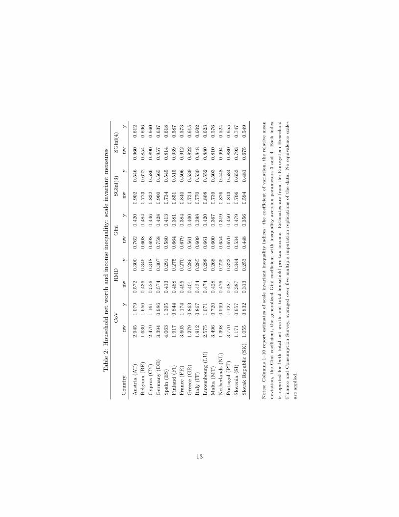
Table2:

Hou

seho

ldne

tworth

andincomeinequa

lity:

scaleinvaria

ntmeasures

CoV

RMD

Gini

SGini(3)

SGini(4)

Cou

ntry

nwy

nwy

nwy

nwy

nwy

Austria

(AT)

2.94

51.07

90.572

0.300

0.762

0.420

0.902

0.546

0.960

0.612

Belgium

(BE)

1.63

01.65

60.436

0.345

0.608

0.484

0.773

0.622

0.854

0.696

Cyp

rus(C

Y)

2.47

91.16

10.526

0.318

0.698

0.446

0.832

0.586

0.890

0.660

German

y(D

E)

3.39

40.98

60.574

0.307

0.758

0.428

0.900

0.565

0.957

0.637

Spain(E

S)4.06

31.39

50.413

0.291

0.580

0.413

0.734

0.545

0.814

0.618

Finland

(FI)

1.91

70.84

40.488

0.275

0.664

0.381

0.851

0.515

0.939

0.587

Fran

ce(F

R)

3.60

51.17

40.495

0.270

0.679

0.384

0.840

0.506

0.912

0.573

Greece(G

R)

1.27

90.86

30.401

0.286

0.561

0.400

0.734

0.539

0.822

0.615

Italy(IT)

1.91

20.86

70.434

0.285

0.609

0.398

0.770

0.530

0.848

0.602

Luxembo

urg(L

U)

2.57

51.07

10.474

0.298

0.661

0.420

0.808

0.552

0.880

0.623

Malta

(MT)

3.496

0.720

0.428

0.268

0.600

0.367

0.739

0.503

0.810

0.576

Netherlan

ds(N

L)1.39

80.59

90.476

0.225

0.654

0.319

0.876

0.448

0.994

0.524

Portuga

l(PT)

3.77

01.12

70.487

0.323

0.670

0.450

0.813

0.584

0.880

0.655

Slovenia

(SI)

1.17

10.95

70.387

0.344

0.534

0.479

0.706

0.653

0.793

0.747

Slovak

Repub

lic(SK)

1.05

50.83

20.313

0.253

0.448

0.356

0.594

0.481

0.675

0.549

Notes:Colum

ns1–10

repo

rtestimates

ofscaleinvarian

tinequa

lityindices:

thecoeffi

cientof

variation,

therelative

mean

deviation,

theGinicoeffi

cient,

thegene

raliz

edGinicoeffi

cientwithinequa

lityaversion

parameters3an

d4.

Eachinde

xis

repo

rted

forbo

thtotalne

tworth

andtotalho

useh

oldpre-taxincome.

Estim

ates

arefrom

theEurosystem

Hou

seho

ldFinan

cean

dCon

sumptionSu

rvey,averaged

over

fivemultipleim

putation

replications

oftheda

ta.Noequivalenc

escales

areap

plied.

13

Table3:

Hou

seho

ldne

tworth

andincomeinequa

lity:

tran

slatio

ninvaria

ntmeasures

√V

Gini

SGini(3)

SGini(4)

Kolm(.125)

Kolm(1)

Kolm(2)

Cou

ntry

nwy

nwy

nwy

nwy

nwy

nwy

nwy

Austria

(AT)

798,56

747

,611

202,85

318,483

239,547

24,040

254,734

26,941

103,314

1,190

324,039

6,049

509,170

9,251

Belgium

(BE)

551,98

682

,062

206,00

223,989

261,792

30,837

289,091

34,458

86,802

2,623

224,246

9,783

329,452

14,062

Cyp

rus(C

Y)

1,662,70

150

,251

468,14

119,291

558,434

25,330

597,507

28,558

318,510

1,284

589,222

6,378

915,030

9,790

German

y(D

E)

662,51

742

,937

147,91

318,621

175,677

24,576

186,873

27,714

63,935

979

133,969

5,649

166,502

9,092

Spain(E

S)1,184,07

843

,721

169,12

812,953

213,922

17,088

237,245

19,348

66,914

728

195,288

3,334

735,039

5,173

Finland

(FI)

309,65

638

,101

107,29

217,212

137,416

23,261

151,642

26,509

28,360

769

96,999

4,636

255,527

7,781

Fran

ce(F

R)

841,34

943

,329

158,48

414,176

196,057

18,680

212,798

21,163

62,350

836

151,268

4,243

195,982

19,834

Greece(G

R)

189,026

23,864

82,855

11,070

108,438

14,918

121,495

17,017

16,171

312

63,987

2,083

87,318

3,632

Italy(IT)

526,06

029

,787

167,71

413,670

211,822

18,218

233,418

20,666

64,618

489

166,215

3,178

203,397

5,365

Luxembo

urg(L

U)

1,82

8,16

989

,574

469,69

235,130

573,973

46,166

624,603

52,149

312,468

3,797

585,056

16,882

726,650

25,049

Malta

(MT)

1,27

9,337

19,048

219,47

29,716

270,412

13,307

296,306

15,243

107,668

205

227,251

1,492

272,174

2,730

Netherlan

ds(N

L)23

7,99

727

,415

111,344

14,588

149,174

20,496

169,273

23,972

25,590

424

112,184

3,110

188,899

5,713

Portuga

l(PT)

576,48

122

,895

102,46

69,130

124,287

11,871

134,598

13,293

36,776

283

82,516

1,722

101,289

2,864

Slovenia

(SI)

174,50

921

,368

79,526

10,707

104,984

14,593

118,026

16,683

14,501

256

60,472

1,839

83,530

3,322

Slovak

Repub

lic(SK)

84,026

11,206

35,706

4,800

47,291

6,475

53,805

7,393

3,563

7017,294

479

25,997

849

Notes:Colum

ns1–14

repo

rtestimates

oftran

slationinvarian

tinequa

lityindices:

thestan

dard

deviation,

theab

solute

Gini

coeffi

cient,

theab

solute

gene

raliz

edS-Ginicoeffi

cientwithinequa

lityaversion

parameters3an

d4,

theKolm

inde

xwithβ

parameter

setto

varyingfraction

sof

thereciprocal

ofmed

ianEurozon

e-wideho

useh

oldne

tworth,na

mely108,782eu

ros

(see

Atkinsonan

dBrand

olini2010).

Eachinde

xis

repo

rted

forbo

thtotalne

tworth

andtotalho

useh

oldpre-taxincome.

Estim

ates

arefrom

theEurosystem

Hou

seho

ldFinan

cean

dCon

sumptionSu

rvey,averaged

over

fivemultipleim

putation

replications

oftheda

ta.Noequivalenc

escales

areap

plied.

14

mean wealth of group P and everyone in group R had the mean wealth of groupR. We then have the following formula (Cowell 2013, Radaelli 2010)

IGini (F ) = πPsPIGini (FP) + πRsRIGini (FR) + IGini (FBetw) , (17)

which gives an exact formula for decomposing the Gini coefficient into the non-overlapping subgroups P and R.

4 Representing wealth distributionsApart from the technical issues involved in measuring the inequality of wealth(discussed in section 3) there is a second issue to be considered before undertak-ing empirical work: whether inequality comparisons are to be made indirectlythrough a statistical “model” of the wealth distribution or directly from theobservations on households or individuals. What we mean by a “model” in thiscontext is a particular functional form that is used to characterise all or part ofthe wealth distribution. Typically such a functional form can be expressed asF (w) = Φ (w; θ1, ..., θk) where Φ is a general class of functions, with an individ-ual member of the class being specified by parameters θ1, ..., θk that are typicallyto be estimated from the data. In effect we have three possible approaches:16

• Non parametric approach: make inequality comparisons using the wealthobservations directly;

• Semi-parametric approach: model a part of the distribution (typically theupper tail) using a functional form and use the wealth observations directlyfor the remainder of the distribution, a procedure that is commonly usedif data are sparse or unreliable in the upper tail;

• Parametric approach: use a model for all of the distribution.

Clearly the second and third approaches require the specification of a functionalform Φ, which immediately raises the question: what makes a “good” functionalform? There are two types of answer. First, how well the models appear to workin representing real-world distributions – this issue is discussed in the remainderof this section. Second, whether there is reason to suppose that a particularfunctional form is linked with a suitable economic model of wealth distribution– this is considered briefly in section 5.1.

4.1 Describing wealth at the top: The Pareto distributionThe upper tail of income and wealth distributions are commonly described bythe Pareto Type I (or “power law”) distribution (Arnold 2008, Maccabelli 2009).The key characteristic of the distribution introduced by Pareto (1895) is the lin-ear relationship between the logarithm of the proportion pw of individuals with

16For overviews of parametric models of income distributions see Bordley et al. (1996),Chotikapanich (2008), Chotikapanich et al. (2012), Kleiber and Kotz (2003), Sarabia (2008).

15

wealth greater than w and the logarithm of w itself. This observation describesa distribution that is said to decay like a power function, a behaviour that char-acterizes “heavy-tailed” distributions.17 In the context of income or wealth, thisrelationship is expected to hold only in the upper tail of the distribution, thatis, above a certain minimum level of wealth w0: the Pareto distribution is amodel for describing top wealth distributions. It has been used for example tomodel wealth in the Forbes ‘rich lists’ (see, e.g., Levy and Solomon 1997, Klasset al. 2006).18

The Pareto Type-I distribution is characterised by the distribution function

F (w) = 1− [w/w]α , w > w (18)

and so has densityf(w) = αwαw−1−α

where α is a parameter that captures the “weight” of the upper tail of thedistribution and w is a parameter that “locates” the distribution. The propor-tion of the population with wealth greater than or equal to w (for w > w) ispw = 1− F (w) and the linearity of the Pareto plot follows from

log pw = logwα − α logw. (19)

The value of α (also called the Pareto index) is related to the inequalityassociated with the Pareto distribution: but note that inequality decreases withα. So, for example in this case the Gini coefficient is given by 1

2α−1 (Kleiberand Kotz 2003). Another useful property of the Pareto distribution is that ifone considers any wealth level w, then the average wealth of those with wealthgreater than w is given by α

α−1w, a relationship known as “van der Wijk’slaw” (Cowell 2011); so in the case of the Pareto distribution another intuitiveinequality concept can be easily defined as the ratio

averagebase = α

1− α ;

which describes, for any base wealth level, how much richer on average are allthose with wealth at or above the the base wealth level (Atkinson, Piketty, andSaez 2011).

Figure 5 shows “Pareto diagrams” for our illustrative HFCS data.19 Eachdiagram shows the logarithm of net worth plotted against log pw for all sampledata. According to (19), all points should be aligned on a straight line withslope −α for Pareto-distributed data. The Pareto diagrams indicate a broadly

17A distribution F is considered “heavy-tailed” if the tail is heavier than the exponential:for all λ > 0 limy→∞ eλy [1− F (y)] =∞.

18Whether the Pareto Type 1 distribution provides satisfactory fit to wealth recorded inthe Forbes rich lists is somewhat controversial; see Ogwang (2013), Brzezinski (2014) andCapehart (2014). The debate revolves around the reliability of Kolmogorov-Smirnov type ofgoodness-of-fit tests when data are measured with measurement error.

19Missing wealth components in HFCS data have been multiply imputed. Figure 5 showsdata from the ‘implicate’ no. 1.

16

linear relationship for the upper quarter of the data in most countries, that isbeyond pw = 0.25. The fit to the Pareto assumption is however not entirelysatisfactory throughout the whole range of net worth: linearity disappears orthe slope changes at the very top, say above pw = 0.99 or even pw = 0.999 orso, that is above the top 1 percent of the samples. We return to this issue inSection 6.3 when discussing data contamination and robustness.

4.2 Overall wealth distributionsThe Pareto distribution just described is a simple, convenient model for sum-marizing the upper tail of a wealth distribution. It is however inappropriate asa model for the overall wealth distribution. A comprehensive functional formobviously requires adequate modeling of the lower part of the distribution too.

Typical options for income distribution analysis include the log-normal,the gamma distribution (Chakraborti and Patriarca 2008), the Singh-Maddala(Singh and Maddala 1976), the Dagum Type I (Dagum 1977, Kleiber 2008) orthe more flexible Generalized Beta distribution of the Second Kind (Jenkins2009, McDonald and Ransom 2008); see Kleiber and Kotz (2003) for a detaileddescription of all these distributions, Bandourian et al. (2003) for a compari-son and Clementi and Gallegati (2005), Dagsvik et al. (2013), Reed and Fan(2008) or Sarabia et al. (2002) for yet other possibilities. All of these modelshave however been developed for “size distributions” and are defined for randomvariables that take on strictly positive values. None of these models is thereforeuseful for wealth distributions that involve zero or negative observations.

A practical approach to address this singularity of wealth distributions maybe to work with “shifted” or “displaced” distributions. This involves addinga shift parameter and specifying the wealth distribution as F s(w) = F (w +c) where F is a conventional size distribution defined on the positive halfline(say a log-normal) and c > 0 is an additional shifting parameter that slidesthe distribution into the negative halfline. For the log-normal, this model isreferred to as the displaced log-normal; see Gottschalk and Danziger (1985) foran application. While simple, this strategy has key drawbacks. First, estimationof the c parameter can be problematic (see the discussion in Aitchison andBrown (1957) or Kleiber and Kotz (2003)). Second, such a specification assumescontinuity at zero that is potentially problematic in applications to net worthdistributions.

A more elaborate approach is developed in Dagum (1990, 1999) who sug-gested combining three separate models: an exponential distribution for nega-tive data, a point-mass at zero and a Dagum Type I distribution for positivedata

FD(w) =

π1 exp(θw) if w < 0π1 + π2 if w = 0

π1 + π2 + (1− π1 − π2)(

1 +(βw

)α)−γif w > 0

(20)

17

where π1 and π2 are the shares of negatives and zeros, α,β and γ are the pa-rameters of a Dagum Type I distribution for positive data (Dagum (1977)) andθ > 0 is the shape parameter for the negative distribution. Lower values of θlead to longer left tail in the negative halfline but the exponential distributionspecification maintains a relatively fast convergence to zero (unlike in the uppertail) “because of institutional and biological bounds to an unlimited increaseof economic agent’s liability” (Dagum 1999, p.248). A more restricted modelcombining the Dagum Type I on the positive halfline and the mass at zerowas presented as the Dagum Type II distribution in Dagum (1977); see alsoKleiber and Kotz (2003). Jenkins and Jäntti (2005) provide an application ofthis model; Jäntti et al. (2012) replace the Dagum specification with a Singh-Maddala model in a parametric model for the joint distribution of income andwealth.

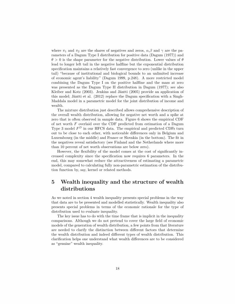
The mixture distribution just described allows comprehensive description ofthe overall wealth distribution, allowing for negative net worth and a spike atzero that is often observed in sample data. Figure 6 shows the empirical CDFof net worth F overlaid over the CDF predicted from estimation of a DagumType 3 model FD in our HFCS data. The empirical and predicted CDFs turnout to be close to each other, with noticeable differences only in Belgium andLuxembourg (in the middle) and France or Slovakia (in the bottom). The fit inthe negatives reveal satisfactory (see Finland and the Netherlands where morethan 10 percent of net worth observations are below zero).

However, the flexibility of the model comes at the cost of significantly in-creased complexity since the specification now requires 6 parameters. In theend, this may somewhat reduce the attractiveness of estimating a parametricmodel, compared to calculating fully non-parametric estimation of the distribu-tion function by, say, kernel or related methods.

5 Wealth inequality and the structure of wealthdistributions

As we noted in section 4 wealth inequality presents special problems in the waythat data are to be presented and modelled statistically. Wealth inequality alsopresents special problems in terms of the economic rationale for the type ofdistribution used to evaluate inequality.

The key issue has to do with the time frame that is implicit in the inequalitycomparisons. Although we do not pretend to cover the large field of economicmodels of the generation of wealth distribution, a few points from that literatureare needed to clarify the distinction between different factors that determinethe wealth distribution and indeed different types of wealth distribution. Thisclarification helps one understand what wealth differences are to be consideredas “genuine” wealth inequality.

18

Wealth inequality and the life cycle issue. Simple life-cycle accumulationmodels predict wealth to be hump shaped over a person’s lifetime (Davies andShorrocks 2000). Empirical evidence shows that assets are typically accumulatedover the working age and decline after retirement age, in response to changingneeds and circumstances; debts tend to peak at younger adult age and declinedrastically in old age (see for example OECD 2008, European Central Bank2013). Some households may have negative net worth at certain points in thelife cycle (for example during a period when they incur mortgage debt thatthey expect to pay off during the time that they are employed). If we take asnapshot of the economy at a particular moment in history the data will typicallypick up individuals at every stage of the adult life cycle. As a consequenceeven if one were to imagine an economy in which individuals were identicalin every respect, other than their date of birth, one would observe substantialwealth inequality that arose purely from this life-cycle process: the extent ofthis apparent inequality would depend on the age distribution. An uncriticallook at the current wealth distribution can therefore pick up wealth differencesbetween persons and between households that are, arguably, not much to do withunderlying inequality of circumstances. This issue also arises in the analysis ofincome distributions, but is more problematic in the case of wealth inequality.

Wealth inequality in the long run. Following this line of reasoning it mightbe thought that all the short-term influences on the wealth distribution shouldeffectively be netted out so as to leave only a wealth distribution that somehowcaptures inequality in the long run. This may be attractive in principle, butpresents a number of important difficulties in practice.

In section 5.1 we consider briefly the issue of long-run modelling and then insection 5.2 we tackle the more modest task of making age adjustments to allowfor the life-cycle effect on wealth dispersion.

5.1 Long-run inequality modellingIf we want to take a truly long-term view of wealth inequality then perhapswe could proceed as follows. Imagine society as a sequence of generations..., n − 1, n, n + 1, ... and consider each person alive at a given moment as therepresentative in generation n of a particular family line or dynasty. Then at-tribute to that representative of generation n a wealth value that represents hisor her lifetime economic position – for example, inherited assets plus a compu-tation of lifetime earnings. Letting Fn denote the distribution function of thisconcept of wealth in generation n, the precise distribution of wealth at a givencalendar time t will be derived from the relevant Fn and information aboutwithin-lifetime wealth profiles and the age structure. The dispersion of wealthimplied by Fn could be taken as a first cut at long-run inequality, purged of allthe short-run – i.e. within lifetime – effects. This “generation-n” distributionwould yield an interpretation of a long-run wealth distribution that graduallyevolves through time as one progresses through the generations n.

19

One might want to go further. To do this, introduce the concept of anequilibrium distribution which can be explained as follows. Represent all theeconomic and social forces that operate on the wealth distribution from gener-ation n to generation n+ 1 by a single process P ; the generation-to-generationdevelopment of the wealth distribution is then written as

FnP7−→ Fn+1. (21)

As a simplified version of this one could imagine that Fn is discrete and givesthe cumulative proportions in each of K wealth categories. Then the processP is simply a transition matrix. It is easy to characterise equilibrium usingequation (21). If there is a distribution F ∗such that

F ∗P7−→ F ∗, (22)

then the self-reproducing F ∗ is the equilibrium distribution for P : if the pro-cess P remains unchanged then F ∗ remains unchanged (Cowell 2014). Noticethat this concept is consistent with long-run wealth mobility within the equilib-rium distribution – it is just the (marginal) distribution of wealth that remainsunchanged through the generations.

This equilibrium distribution is the concept underlying many recent ap-proaches to long-run inequality and can also be understood as a way of rational-ising some of the very early contributions to the literature that used terms suchas “Laws of Distribution”.20 Of course in some cases there exist no F ∗ at all fora given P and, where such a F ∗ does exist, there is no reason to suppose thatit will be representable in a convenient functional form. But for models of Pthat yield a tractable closed-form solution for the equilibrium distribution, F ∗very often turns out to be of the Pareto (type 1) form discussed in section 4.1above. Characterising long-run wealth inequality then becomes a matter of ap-propriately modelling P and of estimating the parameter(s) of the equilibriumdistribution F ∗.

However, the above account is just a sketch, even if it is an attractive sketch.Once one tries to sort out the components of a serious model of wealth inequalityit is clear that the story is inevitably complicated. Sometimes the many forcesthat determine the development of the wealth distribution are summarised in theform of a two-chapter story, the first chapter concentrating on within-lifetime de-cisions, (savings for retirement, labour supply, the acquisition of human capital)and the second consisting of decisions and circumstances relating to connectionsbetween the generations (bequest planning) – see Champernowne and Cowell(1998). But the two-chapter approach is for methodological convenience only:in practice the divide between the two is blurred and one cannot assume thatthe wealth adjustments arising from “Chapter 1 decisions” can be separated outneatly from those that are conventionally considered as “Chapter 2 issues”; for

20See, for example, Pareto (1896, 1965, 2001), Davis (1941), Bernadelli (1944) , Wold andWhittle (1957), Champernowne (1973), Champernowne and Cowell (1998), Cowell (1998),Piketty and Zucman (2014b) and the on-line Appendix to Piketty (2014a).

20

example, it is argued that the observed inequality and heterogeneity of wealthin retirement years is attributable to interaction of decisions from each of thetwo chapters (De Nardi and Yang 2014, Hendricks 2007, Yang 2008); againthe anticipation of a wealth transfers may affect within-lifetime decisions. Thissuggests that trying to examine long-run wealth inequality by filtering out thewithin-lifetime component is a daunting task.

5.2 Age-adjusted wealth inequality measuresHowever a less daunting task is worth considering: making adjustments to mea-sured wealth inequality to take account of the distinctive lifetime pattern ofpersonal wealth holding. The implication of this pattern is that cross-sectionmeasures of wealth inequality at a point in time in a population are shapedby a society’s age structure. Even if everyone had common wealth accumu-lation paths over the life-cycle, wealth at any point in time would turn outto be unequally distributed when pooling observations of individuals of differ-ent age. In practice, there is also much within-cohort heterogeneity in wealthholdings between individuals and heterogeneity in wealth trajectories. Sincewealth-inequality indicators conflate demographic influences of the age struc-ture as well as inequality in life-cycle wealth accumulation, the relevance ofdifferences in cross-section wealth inequality measures across countries or overtime may be questioned (Atkinson 1971, Davies and Shorrocks 2000).

The Gini coefficient within age groups can be connected to the overall Ginicoefficient by the relation

IGini (F ) =A∑a=1

saπaIGini (Fa) + IGini (FBetw) +R (23)

where Fa is the wealth distribution within age group a, sa and πa are respectivelythe population share and the total wealth share of age group a, FBetw is the“between-group”distribution (see section 3.3.4) which in this case is derived byassigning to each individual the mean wealth within their age group, and finallyR captures the degree of overlap between the wealth distributions of the differentage groups. The last term disappears only in the unrealistic case of wealthin each subgroup having strictly non-overlapping support. The decompositionmakes it clear that the overall Gini can be influenced by inequality within agegroups – that may considered of genuine interest – but also by the distributionof population over different age groups, as well as by the differences in meanwealth between age groups which are driven by life-cycle accumulation patternsand changes in wealth holdings over successive birth cohorts.

Variation in inequality within and between age groups is documented inFigure 7. The diagram shows the Gini coefficient calculated within each agegroup IGini (Fa) (the solid lines), along with the population share in each groupsa (the vertical dark grey bars) and the share of total wealth held by each agegroup πa (the vertical light grey bars). The overall Gini coefficient IGini (F )

21

is given by the upper horizontal reference line (dot-dashed) and the between-group Gini IGini (FBetw) is given by the lower reference line (dashed). TheGini coefficient calculated within groups generally declines with age althoughthe decline is not monotone in most countries and in a country like Cyprusit actually increases across age groups. In all countries (except Slovenia) thewealth share of the younger age groups is (substantially) below their populationshares, and the reverse holds for the middle age groups: the extent of thosedeviations is reflected in the level of the between group Gini. Note that thewithin group Gini coefficients are estimated on relatively small samples andare relatively imprecisely estimated: 95 percent confidence intervals are shownby the vertical segments and the shaded area behind total and between groupGinis.21 . Perhaps surprizingly, population shares across the different age groupsdo indeed vary across European countries. For example the share of householdswith reference aged less than 30 ranges from almost 20 percent in Finland toless than 5 percent in Italy.

Various authors have proposed age-adjusted inequality measures to addressthis concern. The idea is simply to derive summary indices purged from theeffect of age. For example Paglin (1975) proposed a simple age-adjusted Giniindex of the form

IPaglinGini(F ) = IGini(F )− IGini (FBetw) (24)

where F is the overall distribution and FBetw is the “between-group” distribu-tion. So IPaglinGini is given by the vertical distance between the two horizontalreference lines in Figure 7. IPaglinGini turns out to be approximately one thirdsmaller than IGini – more so in Luxembourg and less so in Slovenia. Paglinessentially argues that instead of assessing inequality by the area between theLorenz curve and a 45 degree line of perfect equality (a Lorenz curve where ev-eryone has the same wealth), one should calculate the area between the Lorenzcurve and a Lorenz curve calculated after assigning each individuals the meanwealth in his age group. Paglin’s simple proposal turned out to be controversial.A string of comments and replies followed in the American Economic Reviewin 1977, 1979 and 1989 (Danziger et al. 1977, Johnson 1977, Kurien 1977, Mi-narik 1977, Nelson 1977, Paglin 1977, Paglin 1979, Wertz 1979, Formby et al.1989, Paglin 1989). Without fundamentally disagreeing on the basic idea ofage-adjustment, later papers pointed out various weaknesses of IPaglinGini andproposed various corrections or alternatives.

In particular, Wertz (1979) proposed an alternative index defined as

IWertzGini(F ) = 12µ (F )

¨| [w − µ (a (w))]− [w′ − µ (a (w′))] |dF (w) dF (w′)

(25)21Confidence intervals are calculated from 499 bootstrap replications of all estimates on the

basis of the replication weights provided with the HFCS data. Estimates shown in Figure7 are based on the first ‘implicate’ of the multiply imputed HFCS data. Within group Giniestimates are not reported in the figure if the range of the confidence interval is greater than0.5.

22

where µ(a) is the mean wealth among individuals of age a. IWertzGini can becontrasted to the similar formulation of the standard Gini coefficient (10) whichcan be rewritten as

IGini(F ) = 12µ (F )

¨| [w − µ (F )]− [w′ − µ (F )] |dF (w) dF (w′) (26)

where, again, µ is the overall mean wealth (see, e.g., Yitzhaki and Schecht-man (2013) on alternative formulations of the Gini coefficient). The distinctionbetween IWertzGini and IGini is the reference against which individual wealth de-viations are measured. By taking within age group means as reference, IWertzGinicaptures inequality driven by within age group deviations only.

Pudney (1993) suggests a similar approach based on calculations of functionsof mean wealth conditional on individual age but for other inequality functionals(Atkinson indices). More immediately perhaps, one could think of additivelydecomposable inequality measures such as the Generalized Entropy measures– decomposed as in (23) but without the problematic R term. They couldbe used to sort out ‘within’ from ‘between’ age-group factors and compositioneffects across age groups in comparisons of wealth inequality over time or acrosscountries. However the limitations due to the presence of zero and negativenet worth data restricts the applicability of these alternatives to a fairly smallsubclass of inequality measures;22 within the Generalised-Entropy class only ameasure related to the coefficient of variation is likely to be of practical use andeven that may be considered to be too sensitive to outliers in the upper tail.This is one reason for the focus on the Gini coefficient in this literature.

A key limitation of the simple Paglin- or Wertz-type of age-adjustment justdescribed is that additional factors that determine wealth are ignored. This isunproblematic to the extent that these factors are independent of age. However,take the effect education for example: this is both a determinant of earningsand wealth accumulation and is strongly correlated with age in a typical cross-section of the population. To address this, Almås and Mogstad (2012) proposea measure similar to (25) and (26) but where the reference level of wealth forobservation i, instead of µ(ai) or µ, is a counterfactual value given by the averagewealth that would be observed if all the population had age ai but otherwise kepttheir other characteristics at the observed values. This counterfactual referencecaptures differences in wealth by age netted out of the composition effect impliedby the association between age and other factors. Almås and Mogstad (2012)

22See section 3.3 above for a general discussion. The Generalised-Entropy (GE) index ofinequality for a wealth distribution F would be written as

1θ [θ − 1]

ˆ [[w

µ(F )

]θ− 1]

dF (w) ,

where θ is a parameter that may be assigned any real value: higher values of θ make the indexmore sensitive to perturbations at the top of the distribution. It is clear that a GE index willonly be well defined for negative values of w in the special cases where θ is an integer greaterthan 1; the case θ = 2 gives a GE index that is ordinally equivalent to ICV(F ) in equation(8) above. GE indices with θ > 2 are likely to be so over-sensitive to extremely high values ofw as to limit their practical applicability (Cowell and Flachaire 2007).

23

show how the counterfactual can be estimated from predictions based on amultivariate regression model relating wealth to age and other factors.

It turns out that methods for purging inequality from the effects of a fac-tor while holding others constant as in Almås and Mogstad (2012) have beenthe focus of the literature on responsibility and compensation (Fleurbaey andManiquet 2010). Indeed, technically and conceptually, the age-adjustment pro-cedures in wealth inequality bear resemblance to the measures of (in-)equalityof opportunity that attempt to disentangle “fair” and “unfair” inequalities at-tributable to effort, luck or individual a priori circumstances (Almås et al. 2011,Roemer and Trannoy 2015).

To conclude, one qualification about age-adjustments of this sort must bemade. In a cross-section, differences in wealth across age do not necessarilyreflect movements along individual life-cycles alone, but also secular shifts ofthe life-cycle patterns across cohorts. So, adjusting inequality for age doesnot just wipe out differences due to life-cycle positions but also changes inthe life-cycle patterns across cohorts. With cross-section data, nothing muchcan be done to address this. For example Almås and Mogstad (2012) adjustwealth holdings of different cohorts of individuals in their cross-section databased on specific, but very strong assumptions about the evolution of life-cycleaccumulation patterns across cohorts (which is assumed multiplicative, constantover time and homogenous across individual types).

6 Empirical implementationRather than trying to provide an extensive empirical review,23 here we dealwith a more narrowly focused pair of questions: (1) how are the raw materialsfor wealth-inequality comparisons obtained? (2) Given household or individual-level data on wealth, how can analysts make inference about inequality in thedistribution of wealth?

In this section we succinctly summarize issues concerning data, estima-tion and inference and describe standard methods, work-rounds and convenientremedies for potential problems; a more detailed review is available in Cowelland Flachaire (2015).

23For some recent country studies on wealth inequality see the following: Canada (Brzo-zowski et al. 2010), China (He and Huang 2012, Li and Zhao 2008, Ward 2013), Egypt(Alvaredo and Piketty 2014), France (Frémeaux and Piketty 2013; Piketty 2003, 2007a, 2011;Piketty et al. 2006), Germany (Fuchs-Schündeln et al. 2009); India (Banerjee and Piketty2004, 2005; Subramanian and Jayaraj 2008), Ireland (Turner 2010), Italy (Brandolini et al.2004, Mazzaferro and Toso 2009), Japan (Bauer and Mason 1992), Spain (Alvaredo and Saez2006, 2009), Sweden (Bager-Sjogren and Klevmarken 1997), Switzerland (Saez et al. 2007),the UK (Oldfield and Sierminska 2009, Hills et al. 2013), the US (Cagetti and De Nardi 2008;Díaz-Giménez et al. 1997; Juster and Kuester 1991; Kopczuk 2014; Piketty and Saez 2003,2007; Wolff 1995, 2014).

24

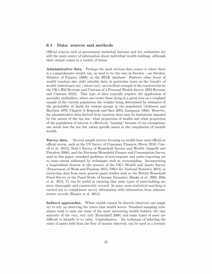
6.1 Data: sources and methodsOfficial sources such as government statistical bureaux and tax authorities arestill the main source of information about individual wealth holdings, althoughtheir output comes in a variety of forms.

Administrative data. Perhaps the most obvious data source is where thereis a comprehensive wealth tax, as used to be the case in Sweden – see Sweden:Ministry of Finance (2006) on the HINK database. However other forms ofwealth taxation also yield valuable data, in particular taxes on the transfer ofwealth (inheritance tax / estate tax): an excellent example is the construction bythe UK’s HM Revenue and Customs of a Personal Wealth Survey (HM Revenueand Customs 2012). This type of data typically requires the application ofmortality multipliers, where one treats those dying in a given year as a weightedsample of the current population the weights being determined by estimates ofthe probability of death for various groups in the population (Atkinson andHarrison 1978, Chapter 3; Kopczuk and Saez 2004; Lampman 1962). However,for administrative data derived from taxation there may be limitations imposedby the nature of the tax law: what proportion of wealth and what proportionof the population of interest is effectively “missing” because of tax exemptions;one needs how the tax law values specific assets in the compilation of taxablewealth.

Survey data. Several sample surveys focusing on wealth have semi-official orofficial status, such as the US Survey of Consumer Finances (Bover 2010, Cow-ell et al. 2012), Italy’s Survey of Household Income and Wealth (Jappelli andPistaferri 2000), and the Eurozone Household Finance and Consumption Surveyused in this paper; standard problems of non-response and under-reporting areto some extent addressed by techniques such as oversampling. Incorporatinga longitudinal element in the manner of the UK’s Wealth and Assets Survey(Department of Work and Pensions 2014, Office for National Statistics 2014) orextracting data from more general panel studies such as the British HouseholdPanel Survey or the Panel Study of Income Dynamics (Banks et al. 2002, Hillset al. 2013, ?) can be useful in ensuring that some types of asset-holding aremore thoroughly and consistently covered. In some cases statistical matching iscarried out to complement survey information with information from adminis-trative records (Rasner et al. 2014).

Indirect approaches. Where wealth cannot be directly observed, one mighttry to rely on observing the traces that wealth leaves. Standard sampling tech-niques tend to miss out some of the most interesting wealth holders, the tinyminority of the very, very rich (Kennickell 2006) and some types of asset aredifficult to identify or to value. Capitalisation – the technique of inferring thevalue of assets held from the flow of income observed, can be used as a forensic

25

device for these types of cases.24 In order to infer the value of the assets byworking backwards from the income generated by the assets clearly one needsreliable microdata on incomes and reliable estimates of the rates of return ondifferent types of asset (Greenwood 1983, King 1927, Saez and Zucman 2014,Stewart 1939). Even when those conditions are met, capitalisation works underthe assumption of uniform rates of return on assets for different wealth groups.Such an assumption is problematic if, say, the wealthy are able to obtain higherreturns on their investments, e.g., though more sophisticated fund management(reference? I think Piketty mentions this point in the book).

Cross-country comparisons. Clearly many of the problems that we havementioned in connection with the standard methods of extracting wealth dataapply with extra force when one attempts to investigate wealth inequality thatinvolves international comparisons or international aggregation. A particularlychallenging example of this is the problem of providing estimates of the globaldistribution of wealth (Davies et al. 2010, Davies et al. 2014): how does onecover the missing population in countries where the data are sparse? In valuingassets in different countries should one use official exchange rate or purchasing-power parity? However some problems of comparability of definitions can beaddressed by using a purpose-built study such as the HFCS used to provideillustrations here (HFCS 2014), or a secondary source of micro-data harmonizedex post such as the Luxembourg Wealth Study (LWS 1994, Sierminska et al.2006).25

6.2 Statistical inference with survey data on wealthNumerous surveys and textbooks have discussed the estimation of income in-equality from micro-data (Cowell 2011) and, of course, many of the conceptsand methods carry over to the measurement of wealth inequality. Yet, empiri-cal analysis of wealth distributions is not just quite the same as the analysis ofincome distributions, and comes with a number of special features (for example,the presence of zero or negative values in net worth) and compounded inferentialproblems (related to the typical heavy tail of wealth distributions).

6.2.1 Inequality statistics: estimation problems

Wealth inequality inference from survey data involves estimation of summarymeasures of inequality, cumulative income functionals, Lorenz ordinates and/or

24This technique requires some heroic assumptions: for example, it is common to assume auniform rate of return across wealth groups, which clearly may be unsatisfactory.

25Examples of wealth comparisons using LWS include Jäntti et al. (2008) and Sierminskaet al. (2008) but of course there is a large number of recent studies that have addressed theissues of international comparability directly (Alvaredo et al. 2013; Atkinson and Piketty2007; Banks et al. 2000; Bover 2010, Ohlsson et al. 2008 Piketty 2005, 2007b, 2014a; Pikettyand Saez 2013, 2014; Piketty and Zucman 2014a, 2014c). Many of these studies draw on theTop Incomes Database http://topincomes.g-mond.parisschoolofeconomics.eu/

26

parameters of functional models from representative household or individual-level micro-data. The shape of wealth distributions with their typically long,heavy right tails challenges standard statistical inference mechanics. Most in-equality functionals of interest are known to be sensitive to extreme values(Cowell and Flachaire 2007, Van Kerm 2007), much more so than quantiles orindicators of central tendency. This has two main consequences.

First, sensitivity to extreme data makes inequality estimates vulnerable todata contamination and measurement error in the tails of the distribution (Cow-ell and Victoria-Feser 1996). Most inequality indicators can in principle bedriven arbitrarily large by a single extreme data point.

Second, simple ‘plug in’ estimators of inequality functionals exhibit finitesample bias and their sampling error remains large and difficult to estimatereliably even in large samples (Cowell and Flachaire 2007, Schluter and vanGarderen 2009, Schluter 2012).

6.2.2 Parametric modelling

The issues just outlined arise in the context of a non-parametric approach toestimation and inference. What if we used instead a parametric-modelling ap-proach, as discussed in section 4?

Estimation of parametric model parameters can usually be undertaken bystandard maximum likelihood methods. However, maximum likelihood estima-tors are known not to be robust to data contamination: parameter estimatescan often be driven arbitrarily large by infinitesimal data contamination, pro-vided this is located at sensitive values of income or net wealth (Hampel et al.1986,Victoria-Feser and Ronchetti 1994). It is therefore desirable to implementestimators robust to the presence of extreme data. One commonly-used option isthe optimal B-robust estimator (OBRE) described by Hampel et al. (1986) andapplied to income distribution models by Victoria-Feser and Ronchetti (1994),Victoria-Feser (2000) and Cowell and Victoria-Feser (2008). More recent ap-proaches are based on Robust Indirect Inference (Genton and Ronchetti 2003).Various robust estimators for the Pareto distribution parameters are reviewedand compared in Brzezinski (2013). Robust estimators of functional form pa-rameters generally require determining a tuning constant for the tradeoff be-tween efficient estimation of the unknown parameters and robustness of theestimator, that is protection of the estimator against extreme data contamina-tion. More of this in section 6.3.2 below.

6.2.3 A general modelling strategy?

Cowell and Victoria-Feser (1996) and Cowell and Victoria-Feser (2002) demon-strate the non-robustness of relative inequality measures and of Lorenz domi-nance comparisons. Using the influence function of appropriate inequality func-tionals (see below), they show how small data contamination in the tails of anincome distribution can ruin inequality inference. Cowell and Flachaire (2007)further illustrate the sensitivity of inequality measures to extreme data and illus-

27

trate the relative sensitivity of different inequality measures (also see Van Kerm2007). Cowell and Flachaire (2007) recommend addressing this concern with asemi-parametric estimation based on parametric modelling of the upper tail ofthe income distribution, an approach adopted in Schluter and Trede (2002) too.The idea of a semi-parametric model combining empirical data for the lower tailand a parametric Pareto distribution model for the upper tail is developed inCowell and Victoria-Feser (2007) to deal with data contamination in point esti-mation and in Davidson and Flachaire (2007) for confidence interval estimationand hypothesis testing using bootstrap methods. Davidson and Flachaire (2007)discuss asymptotic and several standard and non-standard bootstrap methodsfor inference on inequality measures. They show how asymptotic and standardbootstrap methods perform poorly and how semi-parametric bootstrap resam-pling from a semi-parametric model just described can significantly improveinference in large samples. Brzezinski (2013) obtain similar results for estima-tion of “top income shares.” In the semi-parametric bootstrap, resamples arecreated by drawing with replacement from the observed data with given proba-bility β and simulated from a Pareto model fitted to the upper tail of the datawith probability 1− β.26

Note that all of these papers are framed in terms of inference on incomeinequality because, it is argued, income often follows heavy tailed distributions.Clearly, the problems are compounded with wealth distributions that typicallyexhibit heavier upper (and possibly lower) tails than income distributions.

A key tool to study these issues is the influence function. The influence func-tion (IF) of a distribution statistic calculated on distribution F , I(F ), capturesthe impact of a marginal increase in the density of the distribution function atincome z on the value of the statistic. To see this formally, denote F ∈ F the dis-tribution function of interest and assume that H(z) ∈ F is another distributionthat consists just of a single point mass at z. The mixture distribution

G := [1− δ]F + δH(z), 0 ≤ δ ≤ 1 (27)

is a representation of a perturbation of the distribution F by a point mass atz. Then the IF measures the impact of the perturbation at income/wealth z onthe statistic I for an infinitesimal δ

IF(z; I, F ) := limδ↓0

[I(G)− I(F )

δ

]. (28)

The IF therefore captures the sensitivity of the functional I to variations inthe data at different z and interest lies in assessing how the IF evolves when zbecomes large (or small), that is, when the contamination is in the upper (orlower) tail. Furthermore, Hampel et al. (1986) show that, asymptotically, thesampling variance of the distribution functional I(F ) is related to the IF by the

26A different strategy for inference is developed in Schluter and van Garderen (2009) andSchluter (2012) who propose normalizing transformation of the index before application ofthe bootstrap.

28

relationAV (I(F )) =

ˆIF(y; I, F )IF>(y; I, F ) dF (y). (29)

(see also Deville 1999, Osier 2009). So, if the IF of I(F ) increases rapidly forhigh or low z, it will exhibit large sampling variance. Indeed, IF for inequalitymeasures can grow large at the upper tail where data are typically sparse (Cowelland Flachaire 2007). This implies large and imprecisely estimated standarderrors for inequality measures from survey data. This is an issue in incomeinequality estimation, and this is compounded with the heavy tail of wealthdistributions.

To help appreciate the relative influence of income and net worth observa-tions in the tails of the samples, Figure 8 shows the relative influence function(IF (I(F ))/I(F )) for two inequality measures: the Gini coefficient (left) and theshare of total income or wealth held by the richest 5 percent (right) calculatedfrom HFCS data. To help comparison of the curves for income and wealth,the x axis is transformed into fractional ranks: the value of the curves at, say,rank 0.50 shows how much the inequality index would be influenced by an in-finitesimal perturbation at the median of the net worth (respectively income)distribution. The sensitivity of the measures to the extreme high values is well-known. What is not so well appreciated, is the sensitivity of the Gini coefficientto the very small, negative net worth data (marked with crosses on the figure):net worth Gini coefficients are not just driven by the very top, but also by thenet worth of households with negative wealth. Unsurprisingly, this sensitivityto the bottom is absent for the “top 5 percent share.”

6.3 Inference based on semi-parametric modelling of thewealth distributions

One convenient approach to address inferential issues is to substitute the stan-dard fully non-parametric analysis of sample data by a semi-parametric analysiscombining a parametric model for top wealth and observed sample data for thelower part of the distribution. This approach allows addressing several issuesat relatively low computational cost: (i) attenuating the impact of outliers anddata contamination, (ii) improving sampling variance calculation, both analyt-ical and bootstrap-based, and (iii) an issue we have not yet discussed so far,top-coding of data.

6.3.1 The model

A parametric model is used for modelling a proportion β of upper wealth datawhile the empirical distribution function is used directly for the rest of thedistribution (the remaining proportion 1− β of lower wealth). The parametricmodel most commonly used for the upper tail is the Pareto distribution—see

29

Section 4.1. The semi-parametric distribution is then

F̃ (y) =

F (y) y ≤ Q(F ; 1− β)

1− β(

yQ(F ;1−β)

)−αy > Q(F ; 1− β)

. (30)

6.3.2 Estimation of α

Of course the α parameter for the upper tail needs to be estimated from thesample.27 At this stage, issues of the sensitivity of the estimator to data con-tamination come into play. As mentioned in Section 6.2.2, standard maximumlikelihood estimation of the parameter is not “robust” in the sense that param-eter estimates can be driven arbitrarily large by data contamination (Victoria-Feser and Ronchetti 1994). Formally, the influence function of the maximumlikelihood estimator of the Pareto index is unbounded, that is, it can be drivenarbitrarily large by data contamination. Several “robust” alternative estima-tors of the Pareto index have been proposed. From detailed comparison of theperformance of five robust estimators of the Pareto distribution parameter insmall samples, Brzezinski (2013) recommends use of the “probability integraltransform statistic estimator” of Finkelstein et al. (2006) which performs as wellas the generic and more commonly used OBRE (Victoria-Feser and Ronchetti1994) at lower computational cost. In any case, Cowell and Flachaire (2007)find that even with a standard non-robust estimator of α, the semi-parametricmodel provides significant improvement on inference compared to the fully non-parametric approach.

6.3.3 Choice of β

The second key issue is to identify the proportion of the data that ought to bemodelled parametrically, that is, selection of β. Systematic approaches can beadopted to identify the value of β beyond which wealth are effectively Paretodistributed. The Hill plot for example involves estimating the α parameter forall candidate values of β and to select the smallest value of β beyond whichthe estimated parameter stabilizes to a constant (Beirlant et al. 1996). Sophis-ticated approaches account for potential data contamination in this procedureand rely on robust techniques; see for example Dupuis and Victoria-Feser (2006).In practice however, β is generally determined heuristically, selecting by eye theamount of the upper tail that needs to be replaced by inspecting a Pareto di-agram showing the linear relationship between the log of wealth and the log ofthe inverse cumulative distribution function (see Section 4.1).

27Note that α must be assumed to be greater than 2 for the Pareto distribution to havefinite variance.

30

6.3.4 Calculation of inequality measures

The full, semi-parametric estimate of the distribution function is recovered fromthe parameter estimate for the Pareto tail model and sample data for the lowerpart of the distribution using (30). Functionals of interest defined on the semi-parametric distribution F̃ (y) can generally be recovered easily from closed-formexpressions, e.g, the quantile functional is given by (Cowell and Victoria-Feser2007)

Q(F̃ , q) =

Q(F, q) q ≤ 1− β

Q(F ; 1− β)(

1−qβ

)−1/α̂(F̃ )q > 1− β

. (31)

(See Cowell and Flachaire (2015) for additional functionals.) Alternatively, andif no closed form expression is available or tractable, inequality functionals canbe recovered from standard expressions for sample data based on a pseudo-sample composed of (i) the observed data in the lower tail and (ii) randomdraws from the Pareto distribution for the upper tail (Van Kerm 2007). Thenumber of random draws should be sufficiently large to guarantee precision ofthe simulation in the upper tail (it is not limited to the number of sample datain the upper tail) and the randomly drawn observations must be weighted sothat their share in the full pseudo-sample is equal to β. Alternatively, Alfonset al. (2013) use the Pareto model only to identify outlying observations anduse either calibration or single-draw replacement from the Pareto distributionto deal with the few extreme observations identified as outliers.

6.3.5 Semi-parametric bootstrap

Davidson and Flachaire (2007) show that the semi-parametric model helps ad-dressing inference. Constructing bootstrap inference on the basis of the semi-parametric model enhances precision of confidence intervals and tests. The ideais to build bootstrap samples by resampling from F̃ , that is by drawing obser-vations with replacement from the bottom of the sample with probability 1− βand taking observations simulated from the Pareto distribution with probabilityβ. Note that in this procedure, point estimates are still calculated on the basisof the full non-parametric sample (both in the full sample and in the resam-ples) and the semi-parametric bootstrap does not involve re-estimation of theα parameter in each bootstrap sample.

6.3.6 Top-coding

Parametric estimation of the upper tail can finally help addressing top-codingissues. Some micro-data providers do not release income or wealth data in full,but rather top-code data beyond a certain threshold in order to protect theconfidentiality of respondents. This strategy is also a drastic way to preventcontamination of extreme outliers. Such form of censoring can take variousforms (Cowell and Flachaire 2015) but the top-coding just described can be

31

easily addressed with a parametric model. Jenkins et al. (2011) show howmaximum likelihood estimation of the distribution parameters can be adjustedto account for top-coding and then be used to recover uncensored observationsby simulation. See Sologon and Van Kerm (2014) for an application with aPareto upper tail model.

7 ConclusionWealth inequality is a key component of the broad picture of socio-economicinequalities and one that has recently received much attention. A lot of thisattention has been fuelled by the accumulation of evidence on an upward trendin the concentration of wealth among the extremely wealthy (Piketty 2014b,Saez and Zucman 2014).

However, measuring inequality in wealth is not only a matter of estimatingthe size of top shares. With this in mind, our paper has covered a broaderset of concepts and tools available for the analysis of wealth inequality. So,rather than just dealing with inequality in respect of the extremely rich wehave focused on the case of typical survey data where an analyst has accessto data on wealth and its components for a large number of households orindividuals. Analysing wealth inequality is in many ways similar to analysingincome inequality, but it is not an identical exercise. While income inequalitymeasurement methods are now well grounded, some issues specific to empiricalwealth inequality measurement remain problematic.

These issues include (1) the problems of dealing with the presence of a sub-stantial number of negative observations in the wealth distribution, where lia-bilities exceed the value of assets (2) the importance of life cycle accumulationdynamics (3) inferential difficulties that arise from the heavy tail of wealth dis-tributions. The tools that are used to address these issues are not new: theyinclude standard inequality measures, adjustments to empirical wealth distribu-tions and modelling parts of the distribution using functional forms. Howeverthe application of these tools needs perhaps to be better understood in order tothrow light on this important aspect of inequality.

32

ReferencesAitchison, J. and J. A. C. Brown (1957). The Lognormal Distribution. London:

Cambridge University Press.Alfons, A., M. Templ, and P. Filzmoser (2013). Robust estimation of economic

indicators from survey samples based on Pareto tail modelling. Journal ofthe Royal Statistical Society: Series C (Applied Statistics) 62, 271–286.

Almås, I. and M. Mogstad (2012). Older or wealthier? The impact of ageadjustment on wealth inequality. Scandinavian Journal of Economics 114,24–54.

Almås, I., A. W. Cappelen, J. T. Lind, E. . Sørensen, and B. Tungodden(2011). Measuring unfair (in)equality. Journal of Public Economics 95 (7),488–499.

Alvaredo, F., A. B. Atkinson, T. Piketty, and E. Saez (2013). The Top 1Percent in international and historical perspective. Journal of EconomicPerspectives 27, 3–20.

Alvaredo, F. and T. Piketty (2014). Measuring top incomes and inequality inthe Middle East: Data limitations and illustration with the case of Egypt.Working paper, EMOD/Oxford, Paris School of Economics, and Conicet.

Alvaredo, F. and E. Saez (2006). Income and wealth concentration in Spainin a historical and fiscal perspective. Discussion Paper 5836, CEPR.

Alvaredo, F. and E. Saez (2009). Income and wealth concentration in Spainfrom a historical and fiscal perspective. Journal of the European EconomicAssociation 7 (5), 1140–1167.

Amiel, Y., F. A. Cowell, and A. Polovin (1996). Inequality amongst the kib-butzim. Economica 63, S63–S85.

Arnold, B. C. (2008). Pareto and generalized Pareto distributions. InD. Chotikapanich (Ed.), Modeling Income Distributions and LorenzCurves, Chapter 7, pp. 119–146. Springer.

Atkinson, A. B. (1971). The distribution of wealth and the individual lifecycle. Oxford Economic Papers 23, 239–254.

Atkinson, A. B. (1975). The Economics of Inequality (First ed.). Oxford:Clarendon Press.

Atkinson, A. B. and A. Brandolini (2010). On analyzing the world distributionof income. The World Bank Economic Review 24, 1–37.

Atkinson, A. B. and A. J. Harrison (1978). Distribution of Personal Wealthin Britain. Cambridge University Press.

Atkinson, A. B. and T. Piketty (Eds.) (2007). Top Incomes over the 20thCentury: A contrast between continental European and English-speakingcountries. Oxford: Oxford University Press.

33

Atkinson, A. B., T. Piketty, and E. Saez (2011). Top incomes in the long runof history. Journal of Economic Literature 49 (1), 3–71.

Azpitarte, F. (2011). Measurement and identification of asset-poor house-holds: A cross-national comparison of Spain and the United Kingdom.Journal of Economic Inequality 9, 87–110.

Bager-Sjogren, L. and N. A. Klevmarken (1997). Inequality and mobility ofwealth in Sweden 1983/84 - 1992/93. Working Paper 1997:7, Departmentof Economics, Uppsala University.

Bandourian, R., J. B. McDonald, and R. S. Turley (2003). A comparison ofparametric models of income distribution across countries and over time.Estadística 55, 135–152.

Banerjee, A. and T. Piketty (2004). Are the rich growing richer? Evidencefrom Indian tax data. In A. Deaton and V. Kozel (Eds.), Data and dogma:the great Indian poverty debate, pp. 598–611. McMillan Press.

Banerjee, A. and T. Piketty (2005). Top Indian incomes, 1922-2000. WorldBank Economic Review 19, 1–20.

Banks, J., R. Blundell, and J. P. Smith (2000). Wealth inequality in theUnited States and Great Britain. Working Paper WP00/20, The InstituteFor Fiscal Studies, Ridgmount St. London.

Banks, J., Z. Smith, and M. Wakefield (2002). The distribution of finan-cial wealth in the UK: evidence from 2000 BHPS data. Working paperW02/21, Institute for Fiscal Studies.

Bastagli, F. and J. Hills (2013). Wealth accumulation, ageing and houseprices. In J. Hills, F. Bastagli, F. Cowell, H. Glennerster, E. Karagiannaki,and A. McKnight (Eds.), Wealth in the UK: Distribution, Accumulation,and Policy. Oxford: Oxford University Press.

Bauer, J. and A. Mason (1992). The distribution of income and wealth inJapan. Review of Income and Wealth 38, 403–428.

Beirlant, J., P. Vynckier, and J. L. Teugels (1996). Tail index estimation,Pareto quantile plots, and regression diagnostics. Journal of the AmericanStatistical Association 91, 1651–1667.

Bernadelli, H. (1944). The stability of the income distribution. Sankhya 6,351–362.

Berrebi, Z. M. and J. Silber (1985). The Gini coefficient and negative income:a comment. Oxford Economic Papers 37, 525–526.

Bordley, R. F., J. B. McDonald, and A. Mantrala (1996). Something new,something old: Parametric models for the size distribution of income.Journal of Income Distribution 6, 91–103.

Bosmans, K. and F. A. Cowell (2010). The class of absolute decomposableinequality measures. Economics Letters 109, 154–156.

34

Bover, O. (2010). Wealth inequality and household structure: U.S. versusSpain. Review of Income and Wealth 56 (2), 259–290.

Brandolini, A., L. Cannari, G. D’Alessio, and I. Faiella (2004). Householdwealth distribution in Italy in the 1990s. Working paper 414, Bank ofItaly, Economic Research Department.

Brandolini, A., S. Magri, and T. M. Smeeding (2010). Asset-based measure-ment of poverty. Journal of Policy Analysis and Management 29 (2), 267–284.

Brzezinski, M. (2013). Asymptotic and bootstrap inference for top incomeshares. Economics Letters 120, 10–13.

Brzezinski, M. (2014). Do wealth distributions follow power laws? Evidencefrom ‘rich lists’. Physica A: Statistical Mechanics and its Applications 406,155–162.

Brzozowski, M., M. Gervais, P. Klein, and M. Suzuki (2010). Consumption,income, and wealth inequality in Canada. Review of Economic Dynam-ics 13 (1), 52–75.

Cagetti, M. and M. De Nardi (2008). Wealth inequality: Data and models.Macroeconomic Dynamics 12, 285–313.

Caner, A. and E. N. Wolff (2004). Asset poverty in the United States, 1984-99: Evidence from the panel study of income dynamics. Review of Incomeand Wealth 50 (4), 493–518.

Capehart, K. W. (2014). Is the wealth of the world’s billionaires not Paretian?Physica A: Statistical Mechanics and its Applications 395, 255–260.

Carney, S. and W. G. Gale (2001). Asset accumulation among low-incomehouseholds. In T. A. Shapiro and E. N. Wolff (Eds.), Assets for the poor:The benefits of spreading asset ownership, Chapter 5. Russell Sage Foun-dation.

Carter, M. R. and C. B. Barrett (2006). The economics of poverty trapsand persistent poverty: An asset-based approach. Journal of DevelopmentStudies 42 (2), 178–199.

Chakraborti, A. and M. Patriarca (2008). Gamma-distribution and wealthinequality. Pramana 71 (2), 233–243.

Champernowne, D. G. (1973). The Distribution of Income Between Persons.Cambridge University Press.

Champernowne, D. G. and F. A. Cowell (1998). Economic Inequality andIncome Distribution, Chapter 10: Fantastic Models of Wealth and IncomeDistribution, pp. 218–249. Cambridge University Press.

Chen, C.-N., T.-W. Tsaur, and T.-S. Rhai (1982). The Gini coefficient andnegative income. Oxford Economic Papers 34 (11), 473–476.

Chotikapanich, D. (Ed.) (2008). Modeling Income Distributions and LorenzCurves. Springer.

35

Chotikapanich, D., W. E. Griffiths, D. Prasada Rao, and V. Valencia (2012).Global income distributions and inequality, 1993 and 2000: Incorporat-ing country-level inequality modeled with Beta distributions. Review ofEconomics and Statistics 94 (1), 52–73.

Clementi, F. and M. Gallegati (2005). Pareto’s law of income distribution:evidence for Germany, the United Kingdom, and the United States. InA. Chatterjee, S. Yarlagadda, and B. K. Chakrabarti (Eds.), Econophysicsof Wealth Distributions. Berlin: Springer.

Cordoba, J.-C. (2008). U.S. inequality: Debt constraints or incomplete assetmarkets? Journal of Monetary Economics 55, 350–364.

Cowell, F. A. (1998). Inheritance and the distribution of wealth. Distribu-tional Analysis Discussion Paper 34, STICERD, London School of Eco-nomics, London WC2A 2AE.

Cowell, F. A. (2000). Measurement of inequality. In A. B. Atkinson andF. Bourguignon (Eds.), Handbook of Income Distribution, Chapter 2, pp.87–166. New York: Elsevier Science B. V.

Cowell, F. A. (2007). Gini, deprivation and complaints. In G. Betti andA. Lemmi (Eds.), Advances in income inequality and concentration mea-sures, Chapter 3. London: Routledge.

Cowell, F. A. (2011). Measuring Inequality (Third ed.). Oxford: Oxford Uni-versity Press.

Cowell, F. A. (2013). UK wealth inequality in international context. In J. R.Hills (Ed.), Wealth in the UK, Chapter 3. Oxford: Oxford UniversityPress.

Cowell, F. A. (2014). Piketty in the long run. British Journal of Sociology 65,708–720.

Cowell, F. A. (2015). Inequality and poverty measures. In M. D. Adler andM. Fleurbaey (Eds.), Oxford Handbook of Well-Being And Public Policy,Chapter 4. Oxford University Press.

Cowell, F. A., K. E., and A. McKnight (2012). Accounting for cross-countrydifferences in wealth inequality. LWS Working Paper Series 13, LIS DataCentre.

Cowell, F. A. and E. Flachaire (2007). Income distribution and inequalitymeasurement: The problem of extreme values. Journal of Economet-rics 141, 1044–1072.

Cowell, F. A. and E. Flachaire (2015). Statistical methods for distributionalanalysis. In A. B. Atkinson and F. Bourguignon (Eds.), Handbook of In-come Distribution, Volume 2. Elsevier.

Cowell, F. A. and M.-P. Victoria-Feser (1996). Robustness properties of in-equality measures. Econometrica 64, 77–101.

Cowell, F. A. and M.-P. Victoria-Feser (2002). Welfare rankings in the pres-ence of contaminated data. Econometrica 70, 1221–1233.

36

Cowell, F. A. and M.-P. Victoria-Feser (2007). Robust stochastic dominance:A semi-parametric approach. Journal of Economic Inequality 5, 21–37.

Cowell, F. A. and M.-P. Victoria-Feser (2008). Modelling Lorenz curves: ro-bust and semi-parametric issues. In D. Chotikapanich (Ed.), Modeling In-come Distributions and Lorenz Curves, Chapter 13, pp. 241–255. Springer.

Dagsvik, J., Z. Jia, B. H. Vatne, and W. Zhu (2013). Is the Pareto-Lévy lawa good representation of income distributions? Empirical Economics 44,719–737.

Dagum, C. (1977). A new model of personal income distribution: Specificationand estimation. Economie Appliquée 30, 413–436.

Dagum, C. (1990). A model of net wealth distribution specified for negative,null and positive wealth. A case study: Italy. In C. Dagum and M. Zenga(Eds.), Income and Wealth Distribution, Inequality and Poverty, pp. 42–56. Berlin and Heidelberg: Springer.

Dagum, C. (1999). A study of the distributions of income, wealth and humancapital. Revue Européenne des Sciences Sociales 37 (113), 231–268.

Dancelli, L. (1990). On the behaviour of the Zp concentration curve. InC. Dagum and M. Zenga (Eds.), Income and Wealth Distribution, In-equality and Poverty, pp. 111–127. Heidelberg: Springer-Verlag.

Danziger, S., R. Haveman, and E. Smolensky (1977). Comment on Paglin1975. American Economic Review 67, 505–512.

Davidson, R. and E. Flachaire (2007). Asymptotic and bootstrap inferencefor inequality and poverty measures. Journal of Econometrics 141, 141 –166.

Davies, J. B. (2009). Wealth and economic inequality. In W. Salverda, N. B.,and T. M. Smeeding (Eds.), The Oxford Handbook of Economic Inequality,Chapter 6. Oxford University Press.

Davies, J. B., R. Lluberas, and A. F. Shorrocks (2014). Global wealth report2014. The year in review, Credit Suisse Research Institute.

Davies, J. B., S. Sandström, A. Shorrocks, and E. N. Wolff (2010). The leveland distribution of global household wealth. The Economic Journal 121,223–254.

Davies, J. B. and A. F. Shorrocks (2000). The distribution of wealth and itsevolution. In Handbook of Income Distribution. Elsevier B.V.

Davis, H. T. (1941). The Analysis of Economic Time Series. Bloomington,Indiana: the Principia Press.

De Nardi, M. and F. Yang (2014). Bequests and heterogeneity in retirementwealth. European Economic Review 72, 182–196.

Denton, N. A. (2001). Housing as a means of asset accumulation: A goodstrategy for the poor? In T. A. Shapiro and E. N. Wolff (Eds.), Assets forthe poor: The benefits of spreading asset ownership, Chapter 7. RussellSage Foundation.

37

Department of Work and Pensions (2014). Statistics on Household Wealth.London: Department of Work and Pensions.

Deville, J.-C. (1999). Variance estimation for complex statistics and estima-tors: Linearization and residual techniques. Statistics Canada: SurveyMethodology 25, 193–203.

Díaz-Giménez, J., V. Quadrini, and J.-V. Rios-Rull (1997). Dimensions ofinequality: Facts on the U.S. distribution of earnings,income and wealth.Federal Reserve Bank of Minneapolis Quarterly Review 21, 3–21.

Donaldson, D. and J. A. Weymark (1980). A single parameter generalizationof the Gini indices of inequality. Journal of Economic Theory 22, 67–68.

Donaldson, D. and J. A. Weymark (1983). Ethically flexible Gini indices forincome distribution in the continuum. Journal of Economic Theory 29 (4),353–358.

Dupuis, D. J. and M.-P. Victoria-Feser (2006). A robust prediction error cri-terion for Pareto modeling of upper tails. Canadian Journal of Statistics.To appear.

Edlund, L. and W. Kopczuk (2009). Women, wealth, and mobility. AmericanEconomic Review 99, 146–178.

European Central Bank (2013). The eurosystem household finance and con-sumption survey: Results from the first wave. Statistics Paper Series 2,European Central Bank, Frankfurt am Main, Germany.

Finkelstein, M., H. G. Tucker, and J. A. Veeh (2006). Pareto tail index esti-mation revisited. North American Actuarial Journal 10 (1), 1–10.

Fisher, M. G. and B. A. Weber (2004). Does economic vulnerability dependon place of residence? Asset poverty across the rural-urban continuum.Rprc working paper no. 04-01, Rural Poverty Research Center.

Fleurbaey, M. and F. Maniquet (2010). Compensation and responsibility. InK. Arrow, A. Sen, and K. Suzumura (Eds.), Handbook of Social Choiceand Welfare, Volume 2, Chapter 22. North Holland.

Formby, J. P., T. G. Seaks, and W. J. Smith (1989). On the measurement andtrend of inequality: A reconsideration. American Economic Review 79 (1),256–64.

Frémeaux, N. and T. Piketty (2013). GINI country report: Growing inequal-ities and their impacts in France. Working paper, AIAS, Amsterdam In-stitute for Advanced Labour Studies.

Fuchs-Schündeln, N., D. Krueger, and M. Sommer (2009). Inequality trendsfor Germany in the last two decades: A tale of two countries. NBERWorking Paper 15059, National Bureau of Economic Research.

Genton, M. and E. Ronchetti (2003). Robust indirect inference. Journal ofthe American Statistical Association 98, 67–76.

38

Gottschalk, P. and S. Danziger (1985). A framework for evaluating the ef-fects of economic growth and transfers on poverty. American EconomicReview 75 (1), 153–161.

Greenwood, D. (1983). An estimation of U.S. family wealth and its distribu-tion from microdata, 1973. Review of Income and Wealth 29, 23–43.

Hampel, F. R., E. M. Ronchetti, P. J. Rousseeuw, and W. A. Stahel (1986).Robust Statistics: The Approach Based on Influence Functions. New York:John Wiley.

Haveman, R. and E. N. Wolff (2004). The concept and measurement of assetpoverty: Levels, trends and composition for the U.S., 1983-2001. JournalOf Economic Inequality 2, 145–169.

He, X. and Z. Huang (2012). Ownership restructuring, marketization andwealth inequality in urban China: 1995 and 2002. China & World Econ-omy 20 (5), 37–62.

Hendricks, L. (2007). Retirement wealth and lifetime earnings. InternationalEconomic Review 48, 421–456.

HFCS (2014). Household finance and consumption survey. Statistical micro-level database, European Central Bank, Frankfurt am Main, Germany,https://www.ecb.europa.eu/home/html/researcher_hfcn.en.html.

Hills, J., F. Bastagli, F. Cowell, H. Glennerster, E. Karagiannaki, andA. McKnight (2013). Wealth in the UK: distribution, accumulation, andpolicy. Oxford University Press.

HM Revenue and Customs (2012). UK Personal Wealth Statistics. 2008 to2010. HMRC.

Jäntti, M., E. Sierminska, and T. Smeeding (2008). The joint distribution ofhousehold income and wealth: Evidence from the Luxembourg WealthStudy. OECD Social, Employment and Migration Working Paper 65,OECD, Paris.

Jäntti, M., E. Sierminska, and P. Van Kerm (2012). Modelling the joint dis-tribution of income and wealth. Paper Prepared for the 32nd GeneralConference of The International Association for Research in Income andWealth, Boston, USA.

Jäntti, M., E. Sierminska, and P. Van Kerm (2013). The joint distributionof income and wealth. In J. C. Gornick and M. Jäntti (Eds.), IncomeInequality: Economic Disparities and the Middle Class in Affluent Coun-tries, Chapter 11. Palo Alto, California: Stanford University Press.

Jappelli, T. and L. Pistaferri (2000). The dynamics of household wealth ac-cumulation in Italy. Fiscal Studies 21, 269–295.

Jenkins, S. P. (1990). The distribution of wealth: measurement and models.Journal of Economic Surveys 4, 329–360.

Jenkins, S. P. (2009). Distributionally-sensitive inequality indices and theGB2 income distribution. Review of Income and Wealth 55, 392–398.

39

Jenkins, S. P., R. V. Burkhauser, S. Feng, and J. Larrimore (2011, March).Measuring inequality using censored data: A multiple imputation ap-proach. Journal of the Royal Statistical Society, Series A 174 (866), 63–81.

Jenkins, S. P. and M. Jäntti (2005). Methods for summarizing and comparingwealth distributions. ISER Working Paper 2005-05, Institute for Socialand Economic Research, University of Essex, Colchester, UK.

Johnson, W. R. (1977). The measurement and trend of inequality: comment.American Economic Review 67, 502–504.

Juster, F. T. and K. A. Kuester (1991). Differences in the measurement ofwealth, wealth inequality and wealth composition obtained from alterna-tive U.S. wealth surveys. Review of Income and Wealth 37, 33–62.

Kennickell, A. B. (2006). A rolling tide: changes in the distribution of wealthin the US, 1989-2001. In E. N. Wolff (Ed.), International Perspectives onHousehold Wealth, Chapter 2, pp. 19–88. Edward Elgar in Associationwith the Levy Economics Institute.

King, W. I. (1927). Wealth distribution in the continental United States at theclose of 1921. Journal of the American Statistical Association 22, 135–153.

Klass, O. S., O. Biham, M. Levy, O. Malcai, and S. Solomon (2006). TheForbes 400 and the Pareto wealth distribution. Economics Letters 90,290–295.

Kleiber, C. (2008). A guide to the Dagum distributions. In D. Chotikapanich(Ed.), Modeling Income Distributions and Lorenz Curves, Chapter 6, pp.97–118. Springer.

Kleiber, C. and S. Kotz (2003). Statistical Size Distributions in Economicsand Actuarial Sciences. Hoboken. N.J.: John Wiley.

Kolm, S.-C. (1976). Unequal inequalities I. Journal of Economic Theory 12,416–442.

Kopczuk, W. (2014). What do we know about evolution of top wealth sharesin the United States? NBER Working Paper 20734, National Bureau ofEconomic Research.

Kopczuk, W. and E. Saez (2004). Top wealth shares in the United States,1916-2000: Evidence from estate tax returns. National Tax Journal 57,445–487.

Kurien, C. J. (1977). The measurement and trends of inequality: Comment.American Economic Review 67, 512–519. Comment on Paglin 1975.

Lampman, R. J. (1962). The share of top wealth-holders in national wealth1922-1956. Princeton University Press.

Levy, M. and S. Solomon (1997). New evidence for the power-law distributionof wealth. Physica A: Statistical Mechanics and its Applications 242 (1–2),90–94.

40

Li, S. and R. Zhao (2008). Changes in the distribution of wealth in China1995-2002. In J. B. Davies (Ed.), Personal Wealth From A Global Per-spective, Chapter 5, pp. 42–63. Oxford University Press. 93-111.

Lorenz, M. O. (1905). Methods for measuring concentration of wealth. Journalof the American Statistical Association 9, 209–219.

LWS (1994). Luxembourg Wealth Study. Database, LIS, Luxembourg.Maccabelli, T. (2009). Measuring inequality: Pareto’s ambiguous contribu-

tion. History of Political Economy 41, 183–208.Mazzaferro, C. and S. Toso (2009). The distribution of total wealth in Italy:

1991-2002. Review of Income and Wealth 55 (issue 3), 779–802.McDonald, J. B. and M. Ransom (2008). The generalized beta distribution

as a model for the distribution of income: Estimation of related measuresof inequality. In D. Chotikapanich (Ed.), Modeling Income Distributionsand Lorenz Curves, Chapter 8, pp. 147–166. Springer.

Minarik, J. (1977). The measurement and trend of inequality: comment andreply. American Economic Review 67 (6), 513–516.

Moyes, P. (1987). A new concept of Lorenz domination. Economics Letters 23,203–207.

Nelson, E. R. (1977). The measurement and trend of inequality: Comment.American Economic Review 67.

OECD (2008).Growing Unequal? Income Distribution And Poverty In OECDCountries. Organisation For Economic Co-Operation And Development.

OECD (2013). OECD Framework for Statistics on the Distribu-tion of Household Income, Consumption and Wealth. OECD pub-lishing, Organisation for Economic Cooperation and Development,http://www.oecd.org/statistics/302013041e.pdf.

Office for National Statistics (2014). Wealth in Great Britain: Wave 3, 2010-2012. ONS.

Ogwang, T. (2013). Is the wealth of the world’s billionaires Paretian? PhysicaA: Statistical Mechanics and its Applications 392 (4), 757–762.

Ohlsson, H., J. Roine, and D. Waldenström (2008). Long-run changes in theconcentration of wealth: An overview of recent findings. In J. B. Davies(Ed.), Personal Wealth From A Global Perspective, Chapter 2, pp. 42–63.Oxford University Press.

Oldfield, Z. and E. Sierminska (2009). Differences in the measurement andstructure of wealth using alternative data sources: the case of the UK.Journal of Financial Transformation 26, 42–50.

Osier, G. (2009). Variance estimation for complex indicators of poverty andinequality using linearization techniques. Survey Research Methods 3 (3),167–195.

41

Paglin, M. (1975). The measurement and trend of inequality: a basic revision.American Economic Review 65, 598–609.

Paglin, M. (1977). The measurement and trend of inequality: Reply. AmericanEconomic Review 67 (3), 520–31.

Paglin, M. (1979). Reply to Wertz. American Economic Review 79, 663–677.Paglin, M. (1989). On the measurement and trend of inequality: Reply. Amer-

ican Economic Review 79 (1), 265–266.Pareto, V. (1895). La legge della domanda. Giornale degli Economisti (10),

59–68.Pareto, V. (1896). La courbe de la répartition de la richesse. In C. Viret-

Genton (Ed.), Recueil publié par la Faculté de Droit à l’occasion del’exposition nationale suisse, Geneva 1896, pp. 373–387. Lausanne: Uni-versité de Lausanne.

Pareto, V. (1965). Écrits sur La Courbe de la Repartition de la Richesse, Vol-ume 3 of Oeuvres Complètes. Geneva: Librairie Droz. Edited by Busino,G.

Pareto, V. (2001). On the distribution of wealth and income. In M. Baldas-sarri and P. Ciocca (Eds.), Roots of the Italian School of Economics andFinance: From Ferrara (1857) to Einaudi (1944), Volume 2, pp. 231–276.Houndmills: Palgrave.

Piketty, T. (2003). Income inequality in France, 1901-1998. Journal of Polit-ical Economy 111, 1004–1042.

Piketty, T. (2005). Top income shares in the long run: An overview. Journalof the European Economic Association 3 (2-3), 1–11.

Piketty, T. (2007a). Income, wage and wealth inequality in France, 1901-98. In A. B. Atkinson and T. Piketty (Eds.), Top Incomes over the 20thCentury: A contrast between continental European and English-speakingcountries, Chapter 1, pp. 43–81. Oxford University Press.

Piketty, T. (2007b). Top incomes over the 20th century: A summary of mainfindings. In A. B. Atkinson and T. Piketty (Eds.), Top Incomes overthe 20th Century: A contrast between continental European and English-speaking countries, Chapter 1, pp. 1–17. Oxford University Press.

Piketty, T. (2011). On the long-run evolution of inheritance: France 1820-2050. Quarterly Journal of Economics 126, 1071–1132.

Piketty, T. (2014a). Capital in the 21st century. Harvard University Press.Piketty, T. (2014b). Dynamic of inequality. New Left View 85, 103–116.Piketty, T., G. Postel-Vinay, and J.-L. Rosenthal (2006). Wealth concentra-

tion in a developing economy: Paris and France , 1807-1994. AmericanEconomic Review 96 (1), 236–256.

Piketty, T. and E. Saez (2003). Income inequality in the United States, 1913-1998. Quarterly Journal of Economics 118, 1–39.

42

Piketty, T. and E. Saez (2007). Income and wage inequality in the UnitedStates, 1913-2002. In A. B. Atkinson and T. Piketty (Eds.), Top IncomesOver the Twentieth Century. Oxford University Press.

Piketty, T. and E. Saez (2013). Top incomes and the Great Recession: Recentevolutions and policy implications. IMF Economic Review 61 (3), 456–478.

Piketty, T. and E. Saez (2014). Inequality in the long run. Science 344 (6186),838–843.

Piketty, T. and G. Zucman (2014a). Capital is back: Wealth-income ratiosin rich countries 1700-2010. Working paper, Paris School of Economics.

Piketty, T. and G. Zucman (2014b). Wealth and inheritance inthe long run. Working paper, Paris School of Economics,http://piketty.pse.ens.fr/files/PikettyZucman2014HID.pdf.

Piketty, T. and G. Zucman (2014c). Wealth and inheritance in the long run.Working paper, Paris School of Economics, London School of Economics,and UC Berkeley.

Pudney, S. (1993). Income and wealth inequality and the life-cycle. Journalof Applied Econometrics 8, 249–276.

Radaelli, P. (2010). On the decomposition by subgroups of the Gini indexand Zenga’s uniformity and inequality indexes. International StatisticalReview 78 (1), 81–101.

Rank, M. R. and T. A. Hirschl (2010). Estimating the life course dynamicsof asset poverty. Csd working papers no. 10-25, Washington University inSt. Louis.

Rasner, A., J. R. Frick, and M. M. Grabka (2014). Statistical matching ofadministrative and survey data: An application to wealth inequality anal-ysis. Sociological Method & Research 43, 192–224.

Reed, W. J. and W. Fan (2008). New four- and five-parameter models forincome distributions. In D. Chotikapanich (Ed.), Modeling Income Dis-tributions and Lorenz Curves, Chapter 13, pp. 211–224. Springer.

Roemer, J. E. and A. Trannoy (2015). Equality of opportunity. In A. B.Atkinson and F. Bourguignon (Eds.), Handbook of Income Distribution,Volume 2. Elsevier.

Roine, J. and D. Waldenström (2012). On the role of capital gains in Swedishincome inequality. Review of income and wealth 58, 569–587.

Saez, E., T. Piketty, and T. Dell (2007). Income and wealth concentration inSwitzerland over the twentieth century. In A. B. Atkinson and T. Piketty(Eds.), Top Incomes Over the Twentieth Century, Chapter 11, pp. 472–500. Oxford University Press.

Saez, E. and G. Zucman (2014). Wealth inequality in the United States since1913: Evidence from capitalized income tax data. NBER Working Paper20625, National Bureau of Economic Research.

43

Salvaterra, T. (1989). Comparison among concentration curves and indexes insome empirical distributions. In C. Dagum and M. Zenga (Eds.), Incomeand Wealth Distribution, Inequality and Poverty, pp. 194–214. New York:Springer-Verlag.

Sarabia, J. M. (2008). Parametric Lorenz curves: Models and applications.In D. Chotikapanich (Ed.), Modeling Income Distributions and LorenzCurves, Chapter 9, pp. 167–190. Springer.

Sarabia, J. M., E. Castillo, and D. J. Slottje (2002). Lorenz ordering be-tween McDonald’s generalized functions of the income size distribution.Economics Letters 75, 265–270.

Schluter, C. (2012). On the problem of inference for inequality measures forheavy-tailed distributions. The Econometrics Journal 15, 125–153.

Schluter, C. and M. Trede (2002). Tails of Lorenz curves. Journal of Econo-metrics 109, 151–166.

Schluter, C. and K. van Garderen (2009). Edgeworth expansions and normal-izing transforms for inequality measures. Journal of Econometrics 150,16–29.

Shorrocks, A. F. (1983). Ranking income distributions. Economica 50, 3–17.Sierminska, E., A. Brandolini, and T. M. Smeeding (2006). The Luxembourg

Wealth Study - a cross-country comparable database for household wealthresearch. Journal of Economic Inequality 4, 375–383.

Sierminska, E., A. Brandolini, and T. M. Smeeding (2008). Comparing wealthdistribution accross rich countries: First results from the LuxembourgWealth Study. In Household wealth in Italy. Banca d’Italia.

Sierminska, E. and T. Smeeding (2005). Measurement issues in wealth: Equiv-alence scales, accounting framework, and reference unit. "construction andusage of comparable microdata on wealth: the LWS" workshop paper,LWS, Perugia, Italy.

Silos, P. (2007). Housing tenure and wealth distribution in life cycleeconomies. The B.E. Journal of Macroeconomics 7, 1 – 22.

Singh, S. K. and G. S. Maddala (1976). A function for the size distributionof income. Econometrica 44, 963–970.

Sologon, D. M. and P. Van Kerm (2014). Earnings dynamics and inequalitytrends in luxembourg 1988–2009. CEPS/INSTEAD Working Paper 2014-03, CEPS/INSTEAD, Esch/Alzette, Luxembourg.

Stewart, C. (1939). Income Capitalization as a Method of Estimating theDistribution of Wealth by Size Group, Volume 3 of Studies in Income andWealth. New York: National Bureau of Economic Research.

Subramanian, S. and D. Jayaraj (2008). The distribution of household wealthin India. In J. B. Davies (Ed.), Personal Wealth From A Global Perspec-tive, Chapter 6, pp. 112–133. Oxford University Press. 93-111.

44

Sweden: Ministry of Finance (2006). Facts about wealth statistics.Tiefensee, A. and M. M. Grabka (2014). Comparing wealth - data quality

of the HFCS. Discussion Paper 1427, DIW Berlin, German Institute forEconomic Research.

Turner, J. D. (2010). Wealth concentration in the European periphery: Ire-land, 1858-2001. Oxford Economic Papers 62 (1), 1–22.

van de Ven, J. (2001). Distributional limits and the Gini coefficient. Re-search Paper 776, Department of economics, University of Melbourne,Melbourne, Australia.

Van Kerm, P. (2007). Extreme incomes and the estimation of povertyand inequality indicators from EU-SILC. IRISS Working Paper 2007-01,CEPS/INSTEAD, Differdange, Luxembourg.

Vickrey, W. S. (1947). Agenda for Progressive Taxation. Ronald Press.Victoria-Feser, M.-P. (2000). Robust methods for the analysis of income dis-

tribution, inequality and poverty. International Statistical Review 68, 277–293.

Victoria-Feser, M.-P. and E. Ronchetti (1994). Robust methods for personalincome distribution models. Canadian Journal of Statistics 22, 247–258.

Ward, P. (2013). Measuring the level and inequality of wealth: An applicationto China. Review of Income and Wealth, DOI: 10.1111/roiw.12063.

Wertz, K. (1979). The measurement of inequality: comment. American Eco-nomic Review 79, 670–72.

Wold, H. O. A. and P. Whittle (1957). A model explaining the Pareto distri-bution of wealth. Econometrica 25, 591–595.

Wolff, E. N. (1995). Top Heavy: A study of the increasing inequality of wealthin America. 20th Century Fund Press, New York.

Wolff, E. N. (2012). The asset price meltdown and the wealth of the middleclass. Working Paper 18559, National Bureau of Economic Research.

Wolff, E. N. (2014). Household wealth trends in the United States, 1983-2010.Oxford Review of Economic Policy 30, 21–43.

Wolff, E. N. (2015). U.S. pensions in the 2000s: the lost decade? Review ofIncome and Wealth forthcoming.

Wolff, E. N. and A. Zacharias (2009). Household wealth and the measure-ment of economic well-being in the United States. Journal of EconomicInequality 7, 83–115.

Yang, F. (2008). Accounting for the heterogeneity in retirement wealth. Fed-eral Reserve Bank of Minneapolis Working Paper Series 638, Federal Re-serve Bank of Minneapolis.

Yitzhaki, S. (1983). On an extension of the Gini inequality index. Interna-tional Economic Review 24 (10), 617–628.

45

Yitzhaki, S. and I. Olkin (1991). Concentration indices and concentrationcurves. In K. Mosler and M. Scarsini (Eds.), Stochastic Orders and De-cisions under Risk, Volume 19, pp. 380–392. Institute of MathematicalStatistics: Lecture-Notes Monograph Series.

Yitzhaki, S. and E. Schechtman (2013). The Gini Methodology: A StatisticalPrimer. Springer Series in Statistics. Springer.

Zanardi, G. (1990). Constituent of the mean deviations and of the meandifference and concentration scheme. In C. Dagum and M. Zenga (Eds.),Income and Wealth Distribution, Inequality and Poverty, pp. 128–148.Heidelberg: Springer-Verlag.

46

0

1000000

2000000

3000000

0

1000000

2000000

3000000

0

1000000

2000000

3000000

0

1000000

2000000

3000000

0

1000000

2000000

3000000

0 .2 .4 .6 .8 1 0 .2 .4 .6 .8 1 0 .2 .4 .6 .8 1

AT BE CY

DE ES FI

FR GR IT

LU MT NL

PT SI SK

Net worth Income

euro

s

Quantiles

Figure 1: Quantile function for net worth and income (estimates at 19 vingtiles)

47

0

.2

.4

.6

0

.2

.4

.6

0

.2

.4

.6

0

.2

.4

.6

0

.2

.4

.6

0 .2 .4 .6 .8 1 0 .2 .4 .6 .8 1 0 .2 .4 .6 .8 1

AT BE CY

DE ES FI

FR GR IT

LU MT NL

PT SI SK

Net worth Income

Vin

gtile

gro

up s

hare

of t

otal

Vingtile groups

Figure 2: Share of total net worth and income for twenty vingtile groups

48

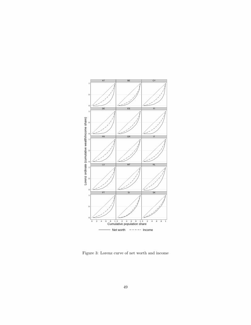
0

.5

1

0

.5

1

0

.5

1

0

.5

1

0

.5

1

0 .2 .4 .6 .8 1 0 .2 .4 .6 .8 1 0 .2 .4 .6 .8 1

AT BE CY

DE ES FI

FR GR IT

LU MT NL

PT SI SK

Net worth Income

Lore

nz o

rdin

ate

(cum

ulat

ive

wea

lth/in

com

e sh

are)

Cumulative population share

Figure 3: Lorenz curve of net worth and income

49

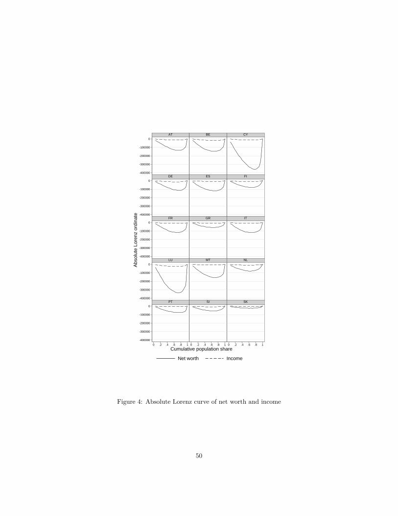
-400000

-300000

-200000

-100000

0

-400000

-300000

-200000

-100000

0

-400000

-300000

-200000

-100000

0

-400000

-300000

-200000

-100000

0

-400000

-300000

-200000

-100000

0

0 .2 .4 .6 .8 1 0 .2 .4 .6 .8 1 0 .2 .4 .6 .8 1

AT BE CY

DE ES FI

FR GR IT

LU MT NL

PT SI SK

Net worth Income

Abs

olut

e Lo

renz

ord

inat

e

Cumulative population share

Figure 4: Absolute Lorenz curve of net worth and income

50

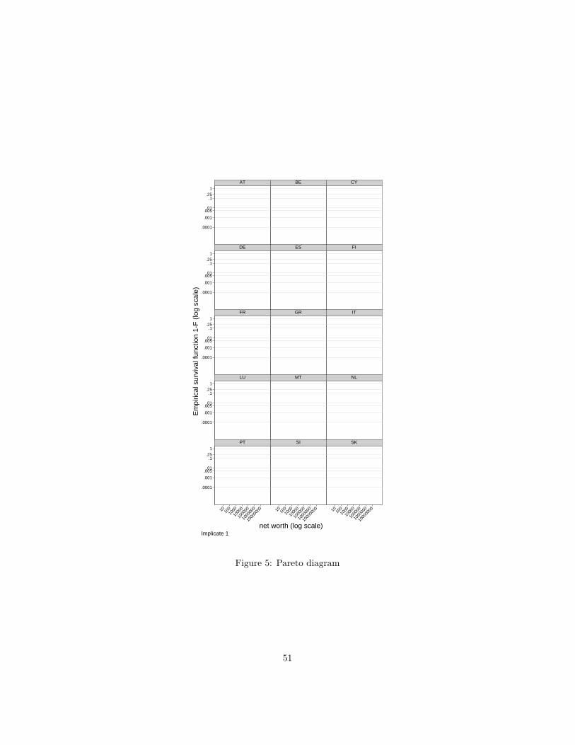
.0001

.001

.005.01

.1.25

1

.0001

.001

.005.01

.1.25

1

.0001

.001

.005.01

.1.25

1

.0001

.001

.005.01

.1.25

1

.0001

.001

.005.01

.1.25

1

10 10010

00

1000

0

1000

00

1000

000

1000

0000 10 10

010

00

1000

0

1000

00

1000

000

1000

0000 10 10

010

00

1000

0

1000

00

1000

000

1000

0000

AT BE CY

DE ES FI

FR GR IT

LU MT NL

PT SI SK

Em

piric

al s

urvi

val f

unct

ion

1-F

(lo

g sc

ale)

net worth (log scale)Implicate 1

Figure 5: Pareto diagram

51

0

.2

.4

.6

.8

1

0

.2

.4

.6

.8

1

0

.2

.4

.6

.8

1

0

.2

.4

.6

.8

1

0

.2

.4

.6

.8

1

-100

0000 0

1000

000

2000

000

-100

0000 0

1000

000

2000

000

-100

0000 0

1000

000

2000

000

AT BE CY

DE ES FI

FR GR IT

LU MT NL

PT SI SK

Empirical CDF Dagum Type III CDF

Mod

el/E

mpi

rical

CD

F

Net worth

Implicate 1

Figure 6: Empirical and Dagum Type 3 CDFs for net worth

52

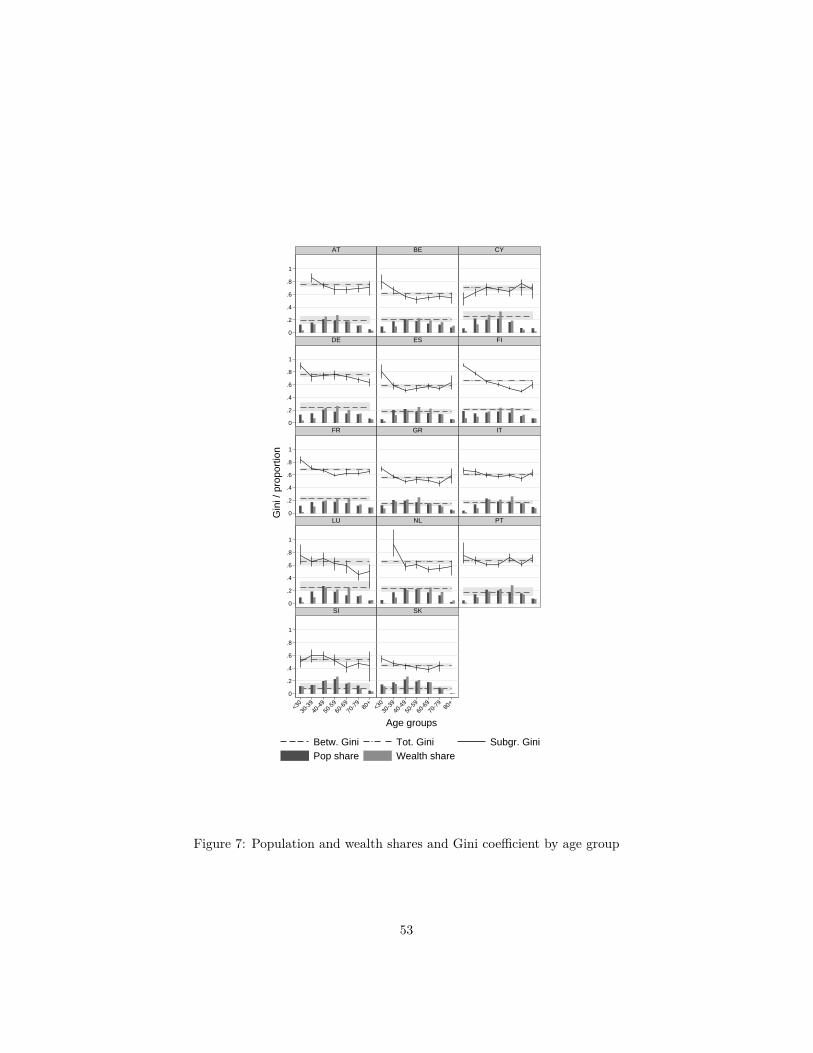
0

.2

.4

.6

.8

1

0

.2

.4

.6

.8

1

0

.2

.4

.6

.8

1

0

.2

.4

.6

.8

1

0

.2

.4

.6

.8

1

<3030

-3940

-4950

-5960

-6970

-79

80+

<3030

-3940

-4950

-5960

-6970

-79

80+

AT BE CY

DE ES FI

FR GR IT

LU NL PT

SI SK

Betw. Gini Tot. Gini Subgr. GiniPop share Wealth share

Gin

i / p

ropo

rtio

n

Age groups

Figure 7: Population and wealth shares and Gini coefficient by age group

53

0

5

10

0

5

10

0

5

10

0

5

10

0

5

10

0 .1 .2 .3 .4 .5 .6 .7 .8 .9 1 0 .1 .2 .3 .4 .5 .6 .7 .8 .9 1 0 .1 .2 .3 .4 .5 .6 .7 .8 .9 1

AT BE CY

DE ES FI

FR GR IT

LU MT NL

PT SI SK

Net worth Disposable income

Rel

ativ

e in

fluen

ce o

n G

ini

Population rank by net worth/income

Implicate 1

-100

0

100

200

-100

0

100

200

-100

0

100

200

-100

0

100

200

-100

0

100

200

0 .1 .2 .3 .4 .5 .6 .7 .8 .9 1 0 .1 .2 .3 .4 .5 .6 .7 .8 .9 1 0 .1 .2 .3 .4 .5 .6 .7 .8 .9 1

AT BE CY

DE ES FI

FR GR IT

LU MT NL

PT SI SK

Net worth Disposable income

Rel

ativ

e in

fluen

ce o

n to

p 5

perc

ent s

hare

Population rank by net worth/income

Implicate 1

Figure 8: Relative influence functions for the Gini coefficient (left) and the top‘vingtile’share (right). Crosses indicate negative net worth.

54