Weak-Shock Interactions with Transonic Laminar MixingLayers of Fuels for High-Speed Propulsion

César Huete∗

University of California, San Diego, La Jolla, California 92093-0411

Javier Urzay†

Stanford University, Stanford, California 94305-3024

and

Antonio L. Sánchez‡ and Forman A. Williams§

University of California, San Diego, La Jolla, California 92093-0411

DOI: 10.2514/1.J054419

This paper extends to transonic mixing layers an analysis of Lighthill (“Reflection at a Laminar Boundary Layer of a

Weak Steady Disturbance to a Supersonic Stream, Neglecting Viscosity and Heat Conduction,” Quarterly Journal of

Mechanics and Applied Mathematics, Vol. 54, No. 1, 1950, pp. 303–325.) on the interaction between weak shocks and

laminar boundary layers. As in that work, the analysis is carried out under linear-inviscid assumptions for the

perturbation field, with streamwise changes of the base flow neglected, as is appropriate given the slenderness of the

mixing-layer flow. The steady-disturbance profile is determined by taking a Fourier transform along the longitudinal

coordinate.Closed-formanalytical functions for thepressure field arederived in the small- and large-wave-number limits,

and vorticity disturbances are obtained as functions of the pressure perturbations. The analysis is particularized to

ethylene–air and hydrogen–air mixing layers, for which the dynamics are of current interest for hypersonic propulsion.

The results provide, in particular, the effective distance of upstream influence of the pressure perturbation in the subsonic

stream. The resulting value, which scales with the thickness of the subsonic layer, is much smaller than the upstream

influence distances encountered in boundary layers. This study may serve as a basis to understand shock-induced

autoignition and flameholding phenomena in simplified versions of non-premixed supersonic-combustion problems.

Nomenclature

Cp = normalized specific heatD = normalized binary diffusion coefficientf1, F1 = physical- and Fourier-space incident pressure

perturbationg1, G1 = physical- and Fourier-space reflected

pressure perturbationJ = normalized fuel-diffusion fluxk = normalized streamwise wave numberL, lm = mixing-layer development distance and thicknessLe = fuel Lewis numberM = Mach numberPr = Prandtl numberp, P = physical- and Fourier-space pressure perturbationsR = normalized densityRe = Reynolds numberT = normalized temperatureU, V = normalized streamwise and transverse velocitiesu, v = normalized streamwise and transverse velocity

perturbationsW = normalized mean molecular weightX, Z = streamwise and transverse global coordinatesx, z = normalized streamwise and transverse local

coordinates

Y, y, Y = base-flow, perturbation, and Fourier- transformedfuel mass fractions

α = thermal-diffusion factorβ = cotangent of Mach angleγ = ratio of specific heatsϵ = normalized perturbation amplitudeη = self-similar variableΘ, θ = physical- and Fourier-space temperature

perturbationsμ = normalized mean viscosityΩ = vorticity production factorω, ϖ = physical- and Fourier-space vorticity perturbations

Subscripts

1 = supersonic airstream2 = subsonic fuel stream

Superscript

0 = dimensional variables

I. Introduction

M IXING layers and shock waves are two different phenomenathat coexist in hypersonic and supersonic propulsion devices.

For instance, in supersonic-combustion ramjets (scramjets), shockwaves are typically generated ahead of the combustion zone, wherethe supersonic incoming flow enters a converging nozzle andinteracts withwedgedwalls and fuel injectors. Along its path throughthe combustor, the flow is subject to complex shock trains andexpansion waves [1].In scramjets, shock waves can interact with the flow in many

different ways. For instance, shocks may disturb the flow near thewalls, leading to sudden transition to turbulence and augmented wallheating in boundary layers. The corresponding shock/boundary-layer interaction problem is one of high practical relevance that hasreceived a large amount of attention in recent years [2–5].A relativelyless known interaction occurs when shocks impinge on chemically

Received29April 2015; revision received10September 2015; accepted forpublication 15 September 2015; published online 7 January 2016. Copyright© 2015 by the authors. Published by the American Institute of AeronauticsandAstronautics, Inc., with permission. Copies of this paper may be made forpersonal or internal use, on condition that the copier pay the $10.00 per-copyfee to the Copyright Clearance Center, Inc., 222 Rosewood Drive, Danvers,MA 01923; include the code 1533-385X/15 and $10.00 in correspondencewith the CCC.

*Postdoctoral Researcher, Department of Mechanical and AerospaceEngineering; chuete@ing.uc3m.es.

†Engineering Research Associate, Center for Turbulence Research.‡Professor, Department of Mechanical and Aerospace Engineering.§Professor, Department ofMechanical and Aerospace Engineering. Fellow

AIAA.

962

AIAA JOURNALVol. 54, No. 3, March 2016

Dow

nloa

ded

by S

TA

NFO

RD

UN

IVE

RSI

TY

on

Mar

ch 3

0, 2

016

| http

://ar

c.ai

aa.o

rg |

DO

I: 1

0.25

14/1

.J05

4419

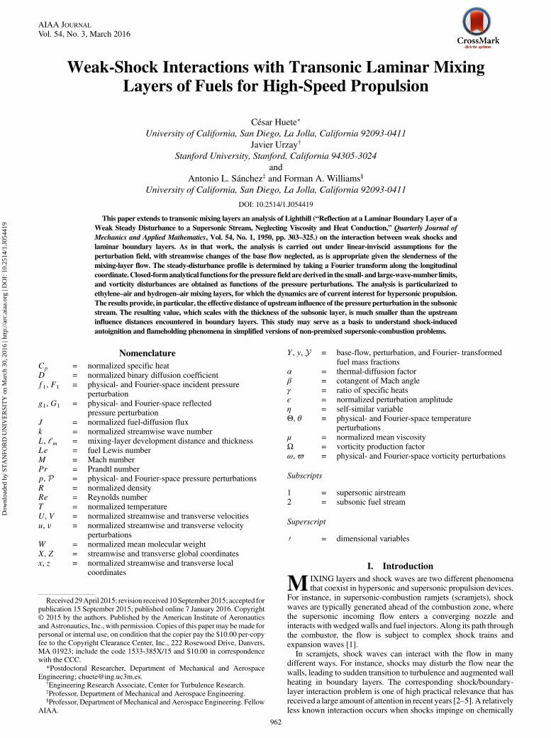
reacting mixing layers of the fuel and oxidizer. To illustrate therelevance of shock/mixing-layer interaction phenomena, consider thefollowing standard fuel-injection configurations employed inscramjets. In one configuration, the shock waves interact with themixing layer that separates the supersonic incoming hot airstream andthe subsonic fuel flow, andwhich is generated downstream from a strutfuel injector (see figures 5 and 11 in [6]). Similarly, in configurationswith jet-in-crossflow fuel injection, a reflected bow shock interactswith themixing layergenerated from the aerodynamics of the fuel jet asit flows into the supersonic incoming hot airstream (see, for instance,figure 4 in [7]). In all cases, since the residence time of the reactants inthe combustor is short in supersonic regimes, ignition typically cannotbe achieved by relying on diffusion and heat conduction alone. Shockwavesmay help, however, to heat themixture and speed up the mixingprocess: with the former arising from the inherent temperature riseacross the shock wave, and the latter associated with the interaction ofthe shock with the nonuniform flow [5–18].Although the aerodynamic interactions described previously are

predominantly encountered in highly turbulent flows in practicalapplications, analytical solutions to related simplified laminarproblems can be advantageous in studying such supersonic-combustion processes, helping to clarify the real configuration, notonly for increasing understanding but also for suggesting scalingconcepts that may prove useful in formulating subgrid-scale models.The present work, which is of that type, pertains to transonic laminarmixing layers formed by fuels employed in supersonic combustionand subjected to impingement by a shock from the airstream, roughlyas illustrated in Fig. 1. As a first step, an inert mixing layer isconsidered, and the shocks are assumed to be sufficiently weak to betreated as linear perturbations of the base flow, with the nonlinearinfluences of finite-amplitude shocks on combustion and the effectsof heat release being deferred to later investigations. A crucial assetfor the present investigation is the earlier work by Lighthill [19,20],which was instrumental in understanding the fundamental dynamicsof weak-shock impingement on wall boundary layers. Initiallypresented in a physical context, it was later shown by Stewartson andWilliams [21] that this type of problem, involving linear (weak-shock) perturbations of a laminar viscous region at large values of theReynolds number Re could be treated rigorously through matchedasymptotic expansions for a Reynolds number approaching infinity,resulting in a triple-deck theory. This has been explained carefully inmore recent reviews, such as that of Nayfeh [22], where therelationships to other triple-deck problems are made clear. Themixing-layer problem to be addressed here turns out to be aparticularly simple version of multiscale problems of this type, forexample, because it is unnecessary to deal with the bottom (low-speed, viscous, incompressible) deck.The objective of this study is to describe, by using asymptotic

analysis, the effect of a weak shock on an inert laminar transonicmixing layer. Particular attention is given to the effect of theperturbations in the nonslender interaction region found around theimpingement point, giving a problem that can be treated usingLighthill’s theory on shock/boundary-layer interaction [19,20].Molecular-transport effects, which determine the slow evolution ofthe mixing-layer flow upstream from the impingement location,have, however, a negligible effect on the perturbations in theinteraction region because the local Reynolds number there is large.Correspondingly, since the streamwise extent of the interactionregion, of the order of the mixing-layer thickness, is much smaller

than the mixing-layer development length, the streamwise variationsof the background flow variables can be neglected when writing thelinearized problem for the perturbations induced by the weak shock.Therefore, for the base flow only, transverse changes in the densityand velocity are considered, whereas the background pressure field isassumed to be constant along and across the mixing layer in the firstapproximation. These approximations engender analytic solutions.The paper is structured as follows: The background laminar mixing

layer and the asymptotic perturbation theory are formulated in Sec. II.The perturbation pressure field is analyzed by means of a Fouriertransformation along the streamwise direction. An ordinary differentialequation for the pressure perturbations, as functions of the transversevariable, is obtained. The asymptotic results for high-frequency and low-frequency disturbances as functions of the transverse coordinate and thefrequency are provided in Sec. III, followed in Sec. IV by an analysis ofthe upstreamdecay of the disturbance.Although the general analysiswillbe performed for a weak pressure perturbation of arbitrary shape, thespecific interaction with a weak step-pressure wave, emulating the weakshock, is addressed inSec.V,where thepressure-perturbationdistributionthroughout the mixing layer is computed and analyzed. The effects thatthe weak shock causes on the vorticity field are analyzed separately inSec. VI. Finally, the conclusions are summarized in Sec. VII.It is relevant to point out that there are three previous investigations

of interactions of oblique shocks with mixing regions, although thespecific transonic problems addressed here have not been treated.Riley [23] employed the same methods adopted here to analyze theinteraction of a shock from a supersonic stream, incident at a fixedplane on a shear layer of infinite extent, in which the Mach numberapproached zero at infinity. Although he did not consider themixing-layer composition and temperature profiles, such as those that weanalyze, instead studying influences of two model transversedistributions of the Mach number, a number of the results of histheory are the same as ours. Moeckel [24] derived a simplifiedmethod for describing shock shapes in purely supersonic mixingregions. The same method was employed later by Buttsworth [25],who attempted computations of vorticity fields in mixing layers ofideal gaseswith similar and different thermodynamic properties, withhis investigation being motivated by the same supersonic-combustion applications that led to our study. All of these excellentcontributions explain methods, not investigated here, for taking intoaccount influences of finite amplitudes of the incident waves.

II. Problem Formulation

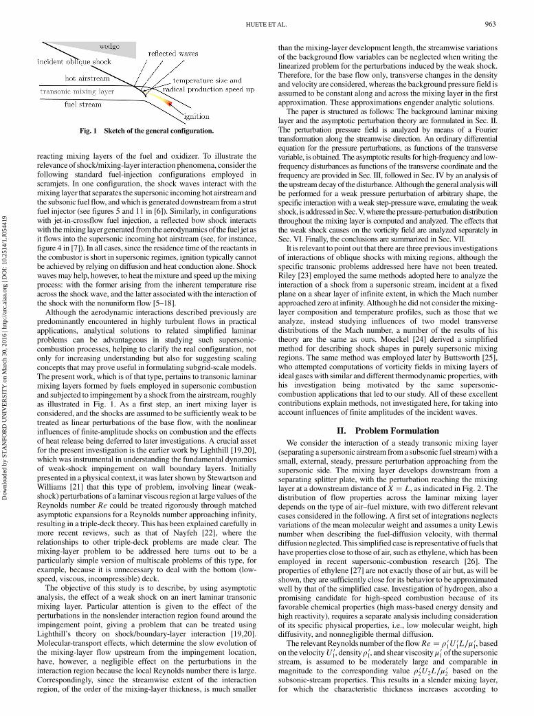
We consider the interaction of a steady transonic mixing layer(separating a supersonic airstream from a subsonic fuel stream)with asmall, external, steady, pressure perturbation approaching from thesupersonic side. The mixing layer develops downstream from aseparating splitter plate, with the perturbation reaching the mixinglayer at a downstream distance of X � L, as indicated in Fig. 2. Thedistribution of flow properties across the laminar mixing layerdepends on the type of air–fuel mixture, with two different relevantcases considered in the following. A first set of integrations neglectsvariations of the mean molecular weight and assumes a unity Lewisnumber when describing the fuel-diffusion velocity, with thermaldiffusion neglected. This simplified case is representative of fuels thathave properties close to those of air, such as ethylene, which has beenemployed in recent supersonic-combustion research [26]. Theproperties of ethylene [27] are not exactly those of air but, as will beshown, they are sufficiently close for its behavior to be approximatedwell by that of the simplified case. Investigation of hydrogen, also apromising candidate for high-speed combustion because of itsfavorable chemical properties (high mass-based energy density andhigh reactivity), requires a separate analysis including considerationof its specific physical properties, i.e., low molecular weight, highdiffusivity, and nonnegligible thermal diffusion.The relevant Reynolds number of the flowRe � ρ 0

1U01L∕μ 0

1, basedon thevelocityU 0

1, density ρ01, and shear viscosity μ

01 of the supersonic

stream, is assumed to be moderately large and comparable inmagnitude to the corresponding value ρ 0

2U2L∕μ 02 based on the

subsonic-stream properties. This results in a slender mixing layer,for which the characteristic thickness increases according to

Fig. 1 Sketch of the general configuration.

HUETE ETAL. 963

Dow

nloa

ded

by S

TA

NFO

RD

UN

IVE

RSI

TY

on

Mar

ch 3

0, 2

016

| http

://ar

c.ai

aa.o

rg |

DO

I: 1

0.25

14/1

.J05

4419

��μ 01∕ρ 0

1�X∕U1�1∕2, reaching a value lm of order Re−1∕2L ≪ L atX � L. Since the relative magnitude of the external pressureperturbation ϵ is assumed to be infinitesimally small, in the firstapproximation, the flow variables are given by those of theunperturbed laminar mixing layer, which is known to possess a self-similar solution, to be described in Sec. II.A. The interaction of theperturbation with the mixing layer occurs in a nonslender region ofcharacteristic size lm, where the relevant local Reynolds number is

ρ 01U

01lm∕μ 0

1 ∼ Re1∕2 ≫ 1. In the double limitRe ≫ 1 and ϵ ≪ 1, theinteraction region can be analyzed following Lighthill’s seminalwork [19,20], by linearizing the conservation equations around thebackground solution, withmolecular-transport terms neglected at theleading order, along with the small streamwise variations of the base

flow, of order Re−1∕2 for the slender mixing layer considered here.

A. Transonic Mixing Layer

In the absence of external perturbations, the transonic mixing layerthat develops downstream from the splitter plate possesses a self-similar solution in terms of the rescaled transverse coordinate

η � Z∕��μ 01∕ρ 0

1�X∕U 01�1∕2. In the description, the longitudinal and

transverse velocity components are scaled with their characteristic

values U 01 and ��μ 0

1∕ρ 01�U 0

1∕X�1∕2 to define the nondimensionalfunctions U�η� and V�η�, whereas the temperature and density arescaledwith their air-sidevaluesT 0

1 and ρ01, respectively, to defineT�η�

and R�η�. The adiabatic pressure disturbances in the interactionregion will be found in the following to be governed by an equationthat depends only on the distribution of the Mach number M�η�across the mixing layer. Since the ratio γ of specific heats isessentially constant in these ideal-gas mixtures, the sound speed isinversely proportional to the square root of the density because thepressure does not vary appreciably across the mixing layer. As aresult, the distribution of Mach numberM�η� can be evaluated fromthe nondimensional velocity and density profiles according to

M�η� � M1U�η�R�η�1∕2 (1)

where M1 > 1 is the Mach number of the airstream, yielding the

relation M2 � M1U2R1∕22 < 1 for the fuel stream Mach number.

Since nitrogen and oxygen are very similar, they will be treated inthe following as a single species, thereby reducing themixing processto that of a binary mixture, with the local composition characterizedin terms of the fuel mass fractionY. The corresponding fuel-diffusionflux, nondimensionalized with �ρ 0

1μ01U

01∕X�1∕2, can be shown to be

expressible in the explicit form [28]

J � −RD

PrLe

�dY

dη� α

Y�1 − Y�T

dT

dη

�(2)

accounting for both species gradient diffusion and thermal diffusion.The latter, known as the Ludwig–Soret effect, exerts significantinfluences in laminar hydrogen–air mixing layers, whereas itsreciprocal Onsager property, known as the Dufour effect, has littleinfluence on the results. Here, Pr � μ 0cp∕λ is the Prandtl number of

the gas mixture, assumed here to be constant and equal to Pr � 0.7,with λ and cp representing the thermal conductivity and the specific

heat at constant pressure of the mixture. The ratio of the thermaldiffusivity λ∕�ρ 0cp� to the fuel–air binary diffusion coefficientD 0 isthe Lewis number, which is a quantity that depends on the mixturecomposition through the variation of λ∕�ρ 0cp� with molecular

weight. Its value in the airstream Le � λ1∕�ρ 01cp1D

01� appears to be

multiplying the Prandtl number in Eq. (2), which includes thedimensionless binary diffusion coefficient D � D 0∕D 0

1, which is afunction of the temperature given in Eq. (8). The thermal-diffusionfactor α [the ratio of the thermal-diffusion coefficient to the productY�1 − Y�ρ 0D 0] will be taken to be constant, which is a sufficientlyaccurate approximation for hydrogen–air mixtures, for which α ≃−0.3 [28].In terms of the aforementioned dimensionless variables, the

conservation equations can be written in the boundary-layer form

−η

2

d

dη�RU� � d

dη�RV� � 0 (3)

R

�V −

η

2U

�dU

dη� d

dη

�μdU

dη

�(4)

RCp

�V −

η

2U

�dT

dη� d

dη

�μCp

Pr

dT

dη

�− �W−1

2 − 1�J dTdη

−α�γ − 1�W2γ

d

dη�WJT� � �γ − 1�M2

1μ

�dU

dη

�2

(5)

R

�V −

η

2U

�dY

dη� −

dJ

dη(6)

where μ � μ 0∕μ 01, Cp � cp∕cp1, and W � W 0∕W 0

1 (W 0 denotingmolecular weights) are the shear viscosity, specific heat, and meanmolecular weight scaled with their airstream values, respectively;and W2 � W 0

2∕W 01.

The preceding equations must be supplemented with the equationof state

RT � W � 1

1� �W−12 − 1�Y (7)

and with the expressions

μ � 1� ��μ 02∕μ 0

1�W−1∕22 − 1�Y

1� �W−1∕22 − 1�Y

Tσ1 ; D � T1�σ1 ; and

Cp � �1� �W−12 − 1�Y�Tσ2 (8)

for the variation with temperature and composition of the transportcoefficients and specific heat. The representativevalues σ1 � 0.7 andσ2 � 0.2 are used in the following for the temperature exponents.The semiempiric expression used for the viscosity of a binarymixture, taken from [29], and that employed for Cp, which follows

from assuming that the molar specific heat at constant pressure isidentical for the fuel and the air, are approximate descriptions thatgive excellent accuracy in many configurations of interest: notablyfor hydrogen–air mixtures. The temperature variations in Eq. (8) andthe assumption that the Prandtl number Pr � μ 0cp∕λ is constant areconsistent with a Lewis number λ∕�ρ 0cpD 0� that has a negligible

temperature dependence and a thermal conductivity that increases

Fig. 2 Sketch of the model problem.

964 HUETE ETAL.

Dow

nloa

ded

by S

TA

NFO

RD

UN

IVE

RSI

TY

on

Mar

ch 3

0, 2

016

| http

://ar

c.ai

aa.o

rg |

DO

I: 1

0.25

14/1

.J05

4419

with temperature according to λ ∝ Tσ1�σ2 . In the simplified case thatapproximates ethylene as the fuel, the dependences on Y disappearfromEqs. (7) and (8), withW � W2 � 1 and μ 0

2 � μ 01, giving μ � 1,

Cp � 1, and, in Eq. (2), J � Tσ1�dY∕dη�∕Pr.The problem reduces to the integration of Eqs. (3–6) supplemented

with Eqs. (7) and (8) and subject to the boundary conditions U � 1,T � 1, and Y � 0 as η → ∞ and U � U2, T � T2, and Y � 1 as

η → −∞, together with the additional boundary condition M �M1UR1∕2 � 1 at η � 0, stating that the arbitrary origin of thetransverse coordinate η is selected to be the sonic point. The resultingdescription is similar to that presented in a previous analysis oftransient hydrogen–air mixing [30]. A distinguishing feature of thepresent analysis is the inclusion of the last two terms in Eq. (5), whichrepresent, respectively, the Dufour effect, by which an energy flux isgenerated by gradients of species concentrations and the heating byviscous dissipation, which is relevant for the transonic conditionsexamined here. Integrations were performed for fuel streamscomposed of hydrogen (Le � 0.3, α � −0.3, W2 � 0.069, andμ 02 � 0.514μ 0

1) and ethylene (Le � 1.2,W2 � 0.97, and μ 02 � 0.6μ 0

1

[27]). Additionally, comparisons were made between ethylene–airand air–airmixing layers (withLe � 1,α � 0,W2 � 1, and μ 0

2 � μ 01

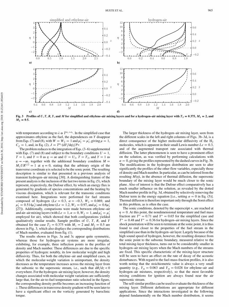
employed for air), which showed that both configurations yieldedqualitatively similar results. Sample profiles of U, T, R, and Yobtained for the case T2 � 0.375 with M1 � 2 and M2 � 0.5 areshown in Fig. 3, which also displays the corresponding distributionsof Mach number, evaluated from Eq. (1).The results shown in Figs. 3a and 3c appear quite symmetric,

whereas those for hydrogen–air systems are more irregular,exhibiting, for example, three inflection points in the profiles ofdensity and Mach number. These differences are due to the specificproperties of hydrogen: notably, its low molecular weight and highdiffusivity. Thus, for both the ethylene–air and simplified cases, inwhich the molecular-weight variation is unimportant, the densitydecreases as the temperature increases across the mixing layer fromthe subsonic to the supersonic stream, i.e., such that dR∕dz < 0everywhere. For the hydrogen–air mixing layer, however, the densitychanges associated with molecular weight variations are sufficientlylarge that, for the air-to-fuel temperature ratio selected in the figure,the corresponding density profile becomes an increasing function ofz. These differences in transverse density gradientwill be seen later tohave a significant effect on the vorticity generated by baroclinictorque.

The larger thickness of the hydrogen–air mixing layer, seen fromthe different scales in the left and right columns of Figs. 3b–3d, is adirect consequence of the higher molecular diffusivity of the H2

molecules, which is apparent in their small Lewis number Le � 0.3,and of the augmented transport rate associated with thermaldiffusion. The latter phenomenon is seen to have a prominent effecton the solution, as was verified by performing calculations withα � 0, giving the profiles represented by the dashed curves in Fig. 3b.The modifications in the hydrogen distribution are seen to altersignificantly the profiles of the other flow variables, especially thoseof density andMach number. In particular, as can be inferred from theresulting M�η�, in the absence of thermal diffusion, the supersonicboundary of the mixing layer would be much closer to the sonicplane. Also of interest is that the Dufour effect comparatively has amuch smaller influence on the solution, as revealed by the dottedMach number profile in Fig. 3d, obtained by selectively removing theDufour term in the energy equation [i.e., setting α � 0 in Eq. (5)].Thermal diffusion is therefore important only through the Soret effectin this problem, as is often the case.The sonic conditions, denoted by the superscript �, are reached at

η � 0. At this point, the nondimensional temperature and fuel massfraction are T� � 0.71 and Y� � 0.65 for the simplified case andT� � 0.48 and Y� � 0.36 for hydrogen–air mixing layers. Since theshock penetrationwill be seen to terminate at the sonic point, it is thusfound to end closer to the properties of the fuel stream in thesimplified case than in the hydrogen–air layer. Largely because of thehigh sound speed of hydrogen, however, the resulting distance fromthe sonic point to the subsonic boundary, measured relative to thetotal mixing-layer thickness, turns out to be considerably smaller inhydrogen–air mixing layers when the Mach numbers of the streamsare fixed. This specific characteristic of the mixing-layer structurewill be seen to have an effect on the rate of decay of the acousticdisturbances. With regard to the fuel-mass-fraction profiles, it is alsoworth noting that the stoichiometric value is always a very smallquantity (e.g., Yst � 0.063 and Yst � 0.028 for ethylene–air andhydrogen–air mixtures, respectively), so that the most favorablemixing conditions for ignition are always found near the airsupersonic stream.The self-similar profiles can be used to evaluate the thickness of the

mixing layer. Different definitions are appropriate for differentapplications. Since the interactions investigated in the followingdepend fundamentally on the Mach number distribution, it seems

a) b)

c) d)

Fig. 3 Profiles of U, T, R, Y, andM for simplified and ethylene–air mixing layers and for a hydrogen–air mixing layer with T2 � 0.375,M1 � 2, andM2 � 0.5.

HUETE ETAL. 965

Dow

nloa

ded

by S

TA

NFO

RD

UN

IVE

RSI

TY

on

Mar

ch 3

0, 2

016

| http

://ar

c.ai

aa.o

rg |

DO

I: 1

0.25

14/1

.J05

4419

appropriate to use the condition of achievement of 99% of thefreestream Mach number as the defining criterion for the location ofthe upper and lower edges of the mixing layer η1 and η2, giving, forinstance, η1 � 4.15 and η2 � −2.85 for the ethylene–air case andη1 � 12.25 and η2 � −3.9 for the hydrogen–air mixing layer shownin Fig. 3. Correspondingly, the analysis yields the value

lm � �η1 − η2���μ 01∕ρ 0

1�L∕U 01�1∕2 (9)

for the mixing-layer thickness at X � L, to be used in the followingas a scale for the interaction region. Because of the initial factor in thisequation, for the conditions of Fig. 3, the hydrogen–air mixing layeris more than twice as thick as the ethylene–air layer. The convectiveMach number, although most commonly employed for turbulentmixing layers, is also known to be readily definable for laminarmixing layers [31], namely,

Mc �U 0

1 −U 02

��γ − 1�cp1T 01�1∕2 � ��γ − 1�cp2

T 02�1∕2

� M1

1 − U2

1� R−1∕22

(10)

which yields 1.05 for the ethylene–air case but only 0.25 forhydrogen–air. This trend is similar to the general one found inturbulent mixing layers, in that mixing-layer thicknesses decreasewith increasing convective Mach numbers [32].

B. Perturbed Pressure Field

The interactions of the external pressure perturbation with themixing layer will be studied in a reference frame for which the originis placed at the intersection of the incident wave with the sonicline, located at �X; Z� � �L; Z��. Using lm as the characteristiclength results in the local coordinates x � �X − L�∕lm andz � �Z − Z��∕lm. In the interaction region, the streamwise variationsof the velocity, density, temperature, and fuel mass fraction of the

unperturbed base flow are small, on the order of Re−1∕2, and they cantherefore be neglected in the first approximation, along with thedepartures of the base-flow pressure from the ambient value p 0

o of

order Re−1. The external pressure perturbation introduced is assumedto be of order ϵp 0

o, leading to relative departures from the base flow oforder ϵ given by

u 0

U 01

� U�z� � ϵu�x; z�; v 0

U 01

� Re−1∕2V�z� � ϵv�x; z�;

ρ 0

ρ 01

� R�z� � ϵρ�x; z�; p 0 − p 0o

γp 0o

� ϵp�x; z� (11)

where the base profilesU�z�,V�z�, andR�z� can be evaluated from theself-similar profiles U�η�, V�η�, and R�η� with use made ofz � η∕�η1 − η2�. The normalized transverse coordinate z is includedfor completeness in the plots of Figs. 3a–3d.Note that, with the scalingintroduced, the edges of the mixing layer z1 � η1∕�η1 − η2� andz2 � η2∕�η1 − η2� are such that z1 − z2 � 1.Since the local Reynolds number in the interaction region

ρ 01U

01lm∕μ 0

1 is large, on the order of Re1∕2 ≫ 1, the perturbations are

governed by the Euler equations, which can be linearized about thebase-flow solution to give

R∂u∂x

�U∂ρ∂x

� vdR

dz� R

∂v∂z

� 0 (12a)

RU∂u∂x

� RvdU

dz� 1

M21

∂p∂x

� 0 (12b)

RU∂v∂x

� 1

M21

∂p∂z

� 0 (12c)

U∂p∂x

� U

R

∂ρ∂x

� v

R

dR

dz(12d)

with the last expressing the conservation of entropy along any givenstreamline. The fuel mass fraction and the temperature are alsomodified by the external pressure perturbation, giving departures thatcan be described by introducingY�z� � ϵy�x; z� andT�z� � ϵθ�x; z�.The perturbation to the mass fraction field, resulting from thedeflection of the streamlines in the interaction region, is determinedby integration of

U∂y∂x

� vdY

dz� 0 (13)

On the other hand, the temperature perturbation θ can be obtainedfrom the condition of isentropic flow:

�γ − 1�U ∂p∂x

� U

T

∂θ∂x

� v

T

dT

dz(14)

or, more directly, from the linearized form of the equation of state

Rθ � γp − Tρ − �W−12 − 1�RTy (15)

in terms of ρ, p, and y.As shown by Lighthill [19], Eq. (12) can be combined to produce a

single equation for the pressure perturbation. The development usessuitable linear combinations of Eqs. (12a), (12b), and (12d) to yield

�1 −M2� ∂p∂x

� ∂∂z

�v

U

�(16)

which leads to

∂2p∂z2

� �1 −M2� ∂2p

∂x2−∂ ln M2

∂z∂p∂z

� 0 (17)

after elimination of v, with use made of Eq. (12c). From Eq. (17),clearly, the solution depends fundamentally on the shape of theMachnumber distributionM�z�.Following Lighthill [19,20] , to simplify the treatment, we

assume that the mixing layer extends across the finite domainz2 < z < z1 and that the base flow is uniform outside. The problemthen reduces to that of integrating Eq. (17) in z2 < z < z1 subject tothe condition that p decays as x → ∞ and to the additionalboundary conditions at z � z1 and z � z2 obtained from matching

with the pressure field in the uniform streams. There,M2 is constantand the pressure-perturbation field obeys the Prandtl–Glauert

equation ∂2p∕∂z2 � �1 −M2�∂2p∕∂x2 � 0, which results in ahyperbolic or elliptic differential equation, depending on whetherthe Mach number is larger or smaller than unity, respectively.In the supersonic stream, the pressure waves follow real charac-

teristic paths C � x β1z � constant, where β1 � �M21 − 1�1∕2,

with the two solutions having different specific domains ofdependence and ranges of influence. The pressure wave in thesupersonic zone can be represented by an incident (known) wave,described by f1�x� β1z�, and a reflected (unknown) wave,described by g1�x − β1z�, so that p � f1�x� β1z� � g1�x − β1z�.This outer pressure field is to be employed when defining theboundary condition at z � z1, given in the following for the Fourieranalysis in Eq. (24). By way of contrast, since Eq. (17) is elliptic forsubsonic flows, the associated characteristic paths are complex,

corresponding to constant values of x iβ2zwith β2 � �1 −M22�1∕2,

causing the entire subsonic-flow domain to be the range of influenceand domain of dependence. Boundedness of the solution as zapproaches −∞ then provides the additional needed boundary

966 HUETE ETAL.

Dow

nloa

ded

by S

TA

NFO

RD

UN

IVE

RSI

TY

on

Mar

ch 3

0, 2

016

| http

://ar

c.ai

aa.o

rg |

DO

I: 1

0.25

14/1

.J05

4419

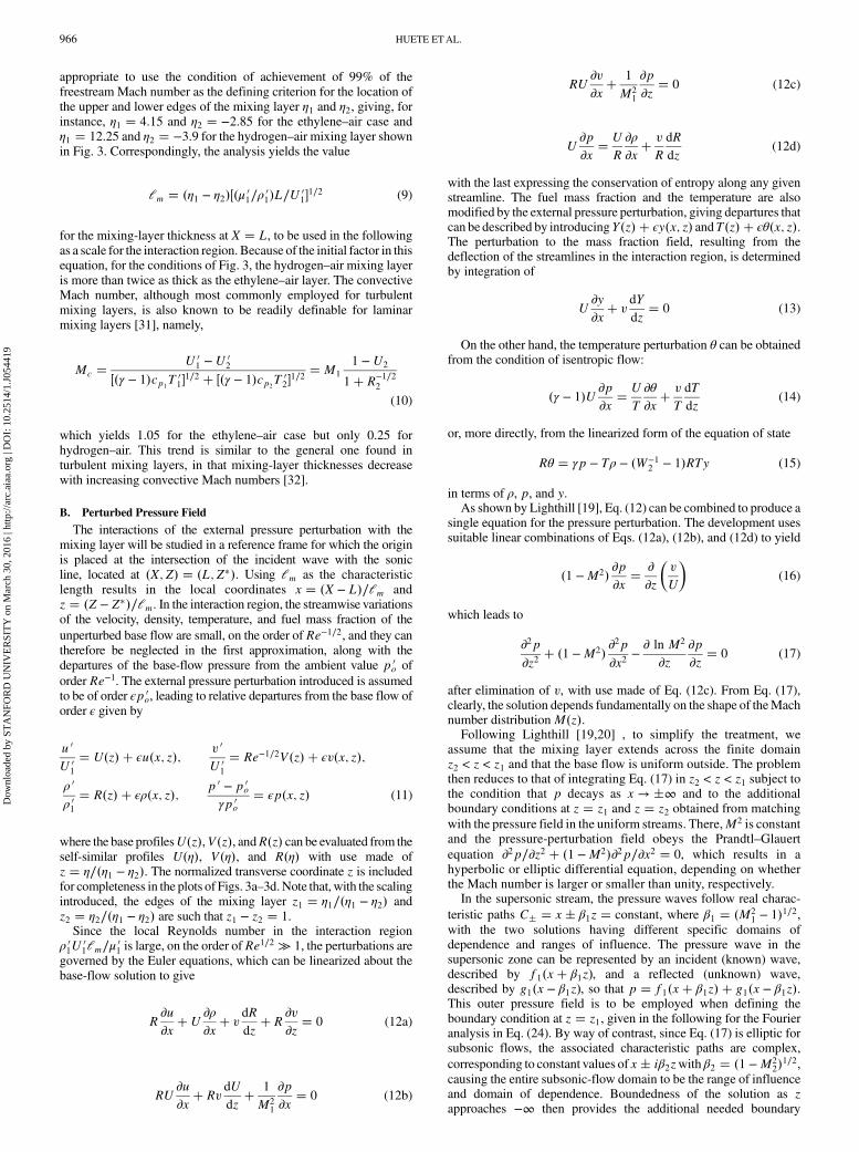
condition at z � z2, given in Eq. (25) in Fourier space, therebycompleting the definition of the pressure-perturbation problem.The model of the interaction is sketched in Fig. 4, where the

incident wave f1 that travels along the path x� β1z � constantinteracts first with the mixing layer at z � z1 and

x � −s1 � −Z

z1

0

�M2 − 1�1∕2 dz

The reflected wave g1 leaves the mixing layer following thecharacteristic x − β1z = constant. The functions g1�x − β1z� andf2�x iβ2z� are to be found by analyzing the interaction with themixing layer for a given function f1�x� β1z�.

C. Solution in Fourier Space

It is useful to transform the partial differential equation [Eq. (17)]into an ordinary differential equation for z by taking a Fouriertransform over the xvariable. The Fourier-transform pressureP�k; z�is defined by its inverse transform

p�x; z� � 1������2π

pZ

∞

−∞eikxP�k; z� dk (18)

where the independent variable k refers to the Fourier wave numberof the pressure disturbances. In the formalism selected here, the

unitary transformation [Eq. (18)] includes a factor 1∕������2π

pthat is not

present in Lighthill’s boundary-layer analysis [19,20], which is adifference to be kept in mind when comparing the boundary-layerand mixing-layer results. In terms of P�k; z�, the governingperturbation equation inside the mixing layer becomes

d2Pdz2

−d ln M2

dz

dPdz

� k2�M2 − 1�P � 0 (19)

Since M is constant in the supersonic and subsonic streams, inthose streams, Eq. (19) reduces to the equation

d2Pdz2

� k2�M2 − 1�P � 0 (20)

The solutions to Eq. (20) are oscillatory in the supersonic stream

(M2 > 1) and exponential in the subsonic stream (M2 < 1). In theformer stream, the pressure field in Fourier space can be written as

P�k; z� � F1�k�eikβ1z �G1�k�e−ikβ1z (21)

where F1�k� describes the incident perturbation, and G1�k� refers tothe corresponding reflected wave. Since the incident perturbation

must be prescribed for any given problem, the function F1�k�eikβ1z isknown. The function G1�k�, however, is to be determined fromEq. (19) by satisfying the boundary condition in the subsonic streamas z approaches negative infinity. SinceG1�k� is unknown, condition(21) must be replaced by a condition that does not involve G1�k�. Asuitable condition, evident from the derivative of Eq. (21), is

dPdz

� iβ1kP � 2iβ1kF1�k�eikβ1z (22)

the right-hand side of which is now a prescribed function.For any given value of k, Eq. (19) can be integrated numerically

from a large positive value of z toward z � −∞ if values ofF1�k� andG1�k� are selected. At large negative values of z, this solution willapproach the solution to the subsonic form of Eq. (20), which can bewritten as

P�k; z� � F2�k�e�jkjβ2z �G2�k�e−jkjβ2z (23)

with the values ofF2�k� andG2�k� determined by the selected valuesof F1�k� and G1�k� through the integration of Eq. (19). Since thesolution must, however, be bounded as z approaches negativeinfinity, G2�k� must vanish. Given F1�k�, there will be a value ofG1�k� that will result in G2�k� � 0. This value of G1�k� willcorrespond to the correct value for the reflected wave. This shootingcomputational approach will provide G1�k� accurately because anyinaccuracies in G1�k� would result in an exponentially divergentsolution as z approaches negative infinity.An alternative to this shooting method is to impose boundary

conditions at sufficiently large but finite values of jzj, as did Lighthill[19]. If these boundaries are placed sufficiently far [i.e., at values ofjzj where Eq. (20) applies because the Mach number is close to itsfreestream values], then the solutions employing Eqs. (22) and (23)with G2�k� � 0 at the computational boundaries will be sufficientlyaccurate. This approach, moreover, facilitates comparisons with theLighthill solutions [19,20]. That approach is therefore selected here,with the values of z1 and z2 associated with the condition ofachievement of 99% of the freestream Mach number, as previouslymentioned.Applying Eq. (22) at z � z1 gives

Pz�k; z1� � iβ1kP�k; z1� � 2iβ1kF1�k�eikβ1z1 (24)

where the subscript z denotes differentiation with respect to thiscoordinate. In the external subsonic zone, where the pressuredistribution [Eq. (23)] holds, the functionG2�k�must vanish to avoida divergent behavior when z → −∞, as previously mentioned.Correspondingly, the boundary condition for P at z � z2 becomes

Pz�k; z2� � β2jkjP�k; z2� (25)

For a given F1�k�, the pressure perturbation in the mixing layerP�k; z� is obtained by integrating Eq. (19) subject to Eqs. (24) and(25). The Fourier transform of the remaining flow variables can bewritten in terms of P and Pz. For instance, the functions Y�k; z� andΘ�k; z�, corresponding to y�x; z� and θ�x; z� in Fourier space, can beevaluated from

Y � −dY

dz

Pz

k2M2(26)

and

Fig. 4 Schematic representation of the incident wave mixing-layer interaction.

HUETE ETAL. 967

Dow

nloa

ded

by S

TA

NFO

RD

UN

IVE

RSI

TY

on

Mar

ch 3

0, 2

016

| http

://ar

c.ai

aa.o

rg |

DO

I: 1

0.25

14/1

.J05

4419

Θ � �γ − 1�TP −dT

dz

Pz

k2M2(27)

obtained from streamwise derivatives of Eqs. (13) and (14) afterEq. (12c) is used to express ∂v∕∂x in terms of the transverse pressuregradient. Also, the solution for P�k; z� can be used to determine thepressure perturbations in the outer streams, including the reflectedwave

G1�k� �ikβ1P�k; z1� − Pz�k; z1�

2ikβ1eikβ1z1 (28)

in the supersonic stream, obtained by appropriately eliminatingF1�k� after differentiatingEq. (21) and evaluating the result at z � z1,as well as the transmitted pressure perturbations

F2�k� � P�k; z2�e−jkjβ2z2 (29)

in the subsonic stream, obtained by evaluating Eq. (23) at z � z2with G2 � 0.

III. Formal Solution in Fourier Space and LimitingAsymptotic Forms

The problemof findingP�k; z� requires numerical integration. Thesmall-scale and large-scale structures of the pressure field can beinvestigated by considering analytic solutions for large and smallvalues of jkj, respectively. To facilitate the analytical development, itis convenient to express the solution formally in terms of twoindependent orthogonal functions,Q andN, defined by the solutionsto Eq. (19) that obey the modified boundary conditions

Q�k; z2� � 1; Qz�k; z2� � 0

N�k; z2� � 0; Nz�k; z2� � 1 (30)

Using these two independent solutions together with the originalboundary conditions [Eqs. (24) and (25)] enables the pressureP�k; z�to be expressed in the form

P�k; z�F1�k�

� 2iβ1k�Q�k; z� � β2jkjN�k; z��E�k; z1; β1; β2�

eikβ1z1 (31)

with

E�k; z1; β1; β2�

given by

E�k; z1; β1; β2� � Qz�k; z1� � iβ1kQ�k; z1�� β2jkj�Nz�k; z1� � iβ1kN�k; z1�� (32)

In particular, Eq. (31) exhibits a linear dependence on the externalperturbationF1�k� and a more complicated dependence on theMachnumber distribution through the functions Q�k; z� and N�k; z�.Solutions will be obtained in the following in the limit jkj ≫ 1 byusing the Wentzel–Kramers–Brillouin (WKB)-like method devel-oped by Langer [33] and in the limit jkj ≪ 1 by introducing regularexpansions in powers of k2 for Q�k; z� and N�k; z�. The formalsolution [Eq. (31)] is also useful to investigate the upstream influenceof the pressure disturbance, for which the rate decays for x → −∞ asdetermined by the negative imaginary zero of the denominator ofEq. (31)with the smallest magnitude jkj. This aspect of the solution isto be investigated in Sec. V, including the differences with theboundary-layer results of Lighthill [19,20].

A. Limit of Large Wave Number

Consideration of the asymptotic limit of k ≫ 1 allows us to explorethe small-scale features of the flow. For the analysis, it is convenientto use, following [19], the earlyWKB-like results obtained byLanger

[33] for equations of the form in Eq. (19). According to Langer’s

analysis, if the two variable coefficients d�ln M2�∕dη and �M2 − 1�are twice differentiable in the interval z2 < z < z1, with the latter

further satisfying �M2 − 1� > 0 for z > 0 and �M2 − 1� < 0 for z < 0,as is the case for the transonic mixing layer, then at the leading orderin the limit k ≫ 1, any solution toEq. (19) can be expressed as a linearcombination of the functions

fa �������2π

pM

jsj1∕6jβj1∕2 �ks�

1∕3J−1∕3�ks�;

fb �������2π

pM

jsj5∕6jβj1∕2 �ks�

−1∕3J1∕3�ks�sign�z� (33)

in which

β � �M2 − 1�1∕2; and s �Z

z

0

β�z 0� dz 0 (34)

with z 0 being a dummy integration variable and Jν representingBessel functions of the first kind. The stretched coordinate s is real inthe supersonic domain z > 0 but imaginary for z < 0. Its value atz � z1 is

s � s1 �Z

z1

0

β�z� dz

whereas that at the subsonic edge is given by s � �is2, where

s2 �Z

0

z2

�1 −M2�1∕2 dz (35)

Equations (33) simplify for values of s such that jksj ≫ 1,corresponding to any fixed transverse location z away from the sonic

line as jkj → ∞, in that the functions �ks�1∕3J∓1∕3�ks� can be

replaced by their asymptotic expressions for large values of theargument, leading to

fa � Mjsj1∕6jβj1∕2

�eiks

�iks�1∕6 �e−iks

�−iks�1∕6�;

fb � Mjsj5∕6jβj1∕2

�eiks

�iks�5∕6 �e−iks

�−iks�5∕6�sign�z� (36)

The constants of integration

CQa �k� � 1

2���3

p�����β2

pM2

�k1∕6eks2 � �−k�1∕6e−ks2� (37a)

CQb �k� �

1

2���3

p�����β2

pM2

�k5∕6eks2 � �−k�5∕6e−ks2 � (37b)

CNa �k� �

1

2���3

p 1

k�����β2

pM2

�k1∕6eks2 − �−k�1∕6e−ks2� (37c)

CNb �k� �

1

2���3

p 1

k�����β2

pM2

�k5∕6eks2 − �−k�5∕6e−ks2� (37d)

that complete the determination of Q � CQa fa � CQ

b fb and N �CNa fa � CN

b fb are obtained by imposing the boundary conditions[Eq. (30)] at the subsonic edge of themixing layer, with the simplifiedexpressions of Eq. (36) used in the evaluations, as is appropriate awayfrom the sonic point. These simplified expressions can also be used to

968 HUETE ETAL.

Dow

nloa

ded

by S

TA

NFO

RD

UN

IVE

RSI

TY

on

Mar

ch 3

0, 2

016

| http

://ar

c.ai

aa.o

rg |

DO

I: 1

0.25

14/1

.J05

4419

evaluate the denominator of Eq. (31), which involves values of thefunctions and their derivatives at the supersonic edge of the mixinglayer, whereas the complete expressions of Eq. (33) must be used forcomputing the functions Q and N appearing in the numerator, if asolution that is valid across the whole mixing layer is to be derived.This evaluation procedure provides

P�k;z�F1�k�

�M2

�����β1

pM1

�����β2

p CQa fa�CQ

b fb� β2jkj�CNa fa �CN

b fb�k cosh�ks2 − iπ∕4�� jkj sinh�ks2 − iπ∕4�ke

ik�β1z1−s1�

(38)

as a uniformly valid expression for the transverse distribution ofpressure perturbation for k ≫ 1, giving, in particular,

P�k; 0�F1�k�

� 21∕3���π

p32∕3�− 1

3�!

�����β1

p

M1�Mz�0��1∕6�1� i sign�k��jkj1∕6eik�β1z1−s1�

(39)

for the corresponding variation of the pressure at the sonic line z � 0,which is seen to exhibit a weak dependence on the local Machnumber gradient Mz�0� � �dM∕dz�jz�0.Away from the sonic point (i.e., for z such that jksj ≫ 1), one may

use Eq. (36) to evaluate fa and fb in Eq. (38), yielding the simplifiedexpressions

P�k; z�F1�k�

������β1β

sM

M1

�eiks � isign�k�e−iks�eik�β1z1−s1� (40)

for z ≫ jkj−1, where the pressure is oscillatory, and

P�k; z�F1�k�

����������β12jβj

sM

M1

�1� isign�k��e−jkjjsjeik�β1z1−s1� (41)

for −z ≫ jkj−1, where the pressure decays exponentially forincreasing distances from the sonic line. Correspondingly, the largewave number components of the reflected and transmitted waves canbe obtained by substituting Eq. (40) into Eq. (28) to give

G1�k� � isign�k�e2ik�β1z1−s1�F1�k� (42)

and Eq. (41) into Eq. (29) to give

F2�k� ���������β12β2

sM2

M1

�1� isign�k��ejkj�β2z2−s2�eik�β1z1−s1�F1�k� (43)

In consonance with Riley [23], the results at a leading order in thelimit jkj ≫ 1 indicate that the pressure distribution across the mixinglayer resulting from the external perturbation becomes largely inde-pendent of the boundary condition at the lower edge. Correspon-dingly, the distribution ofP across themixing layer, given in Eq. (38)for jkj ≫ 1, is identical to that computed by Lighthill [19,20] for aboundary-layer flow with the same Mach number distributionM�z�,except in a region of characteristic thickness jkj−1 near the loweredge, where significant differences appear. As a result, although thepressure perturbation at the sonic line, given inEq. (39), and the shapeof the reflected wave, given in Eq. (42), are identical for a mixinglayer and a boundary layer that have the sameM�z� in the supersonicdomain, the corresponding pressure at the mixing-layer subsonicboundary, obtained by evaluating Eq. (41) at z � z2, is half the valuepredicted by Lighthill at the boundary-layer wall, given by equation23 in [20]. Clearly, these differences in pressure magnitude areassociated with the different nature of the boundary, with theconfinement exerted by the wall resulting in higher pressures.

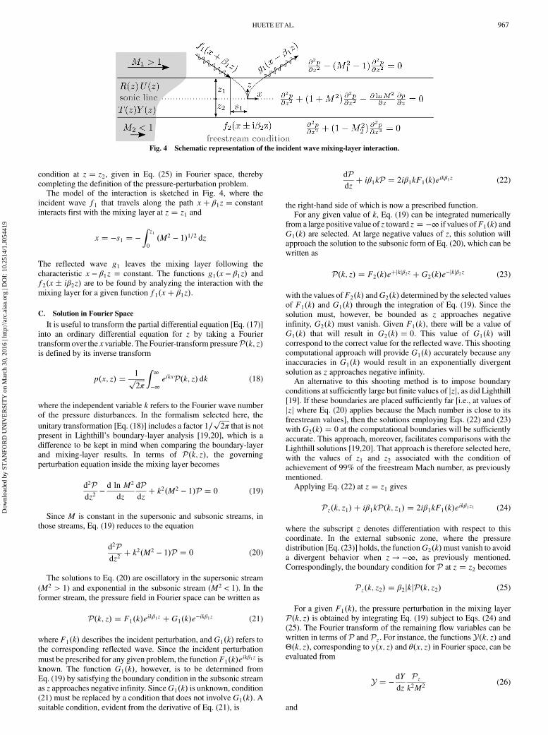
The accuracy of the aforementioned large wave-numberasymptotic predictions is tested in Fig. 5, which compares thevariation with z of the real part of P∕F1 obtained by numericalintegration of Eq. (19) subject to Eqs. (24) and (25) with thatevaluated with use made of Eq. (38) for the hydrogen–air mixinglayer of Fig. 3d. For the value k � 30 selected, the differences areseen to be very small everywhere. The separate predictions given inEqs. (40) and (41) for the pressure disturbances in the supersonic andsubsonic domains are also included in the plot. As expected, thesesimplified expressions give a sufficiently accurate description awayfrom the sonic point, but they break down as M → 1 in the regionwhere jksj is no longer small, where Eqs. (40) and (41) predict anerroneous pressure divergence resulting from the associated factors1∕

���β

pand 1∕

������jβjp.

The asymptotic results are further tested in Figs. 6a–6c, whichcompare the variation with wave number of the real part of P∕F1 atz � �z1; 0; z2� obtained numerically with those determined fromevaluations of the analytic predictions, given in Eq. (39) for thepressure at the sonic line z � 0 and in Eqs. (40) and (41) for thepressure at the supersonic and subsonic mixing-layer boundaries,respectively (results corresponding to the small wave-number limit,to be discussed in the following, are also included in the figure). Ascan be seen, at all three locations, the asymptotic predictions remainreasonably accurate until the wave number decreases to values oforder unity.The large wave-number predictions given previously can also be

used to evaluate the perturbations to the other flow variables, e.g.,those of the fuelmass fraction and temperature, given in Eqs. (26) and

Fig. 5 Real part ofP∕F1�k � 30� by computing Eq. (19) (thick, black,

solid curves), Eq. (38) (thin, gray, solid curves) and in Eqs. (40) and (41)(dashed curves).

a)

b)

c)

Fig. 6 Real part of the function P∕F1�k� at z � z1 a), z � 0 b), andz � z2 c), by computing Eq. (19) (solid curves) and the small and largelimits (dashed curves).

HUETE ETAL. 969

Dow

nloa

ded

by S

TA

NFO

RD

UN

IVE

RSI

TY

on

Mar

ch 3

0, 2

016

| http

://ar

c.ai

aa.o

rg |

DO

I: 1

0.25

14/1

.J05

4419

(27). As expected, the deflection of the streamlines has a negligibleinfluence on the large wave-number component of the solution sothat, in the limit jkj ≫ 1, the mass fraction perturbation Y vanishes,whereas the temperature perturbation [Eq. (27)] reduces to the localisentropic balance Θ∕T � �γ − 1�P.

B. Limit of Small Wave Number

In the opposite limit jkj ≪ 1, the solution can be obtained byintroducing the expansions Q�k; z� � Q0�z� � k2Q1�z�� · · · andN�k; z� � N0�z� � k2N1�z�� · · · into Eq. (19) and solvingsequentially the equations that appear at different orders in powersof k2. The development is facilitated by writing Eq. (19) in thecompact form

d

dz

�M−2 dP

dz

�� k2�M−2 − 1�P (44)

The right-hand-side term is absent in the equation at leading order

d

dz

�M−2 dP0

dz

�� 0 (45)

where P0 is used to denote either one of the leading-order terms Q0

and N0 so that straightforward integration with boundary conditionsQ0 − 1 � �Q0�z � 0 and N0 � �N0�z − 1 � 0 at z � z2 provides

Q0 � 1 and N0 �Z

z

z2

�M

M2

�2

dz 0 (46)

At the following order, we find

d

dz

�M−2 dP1

dz

�� k2�M−2 − 1�P0 (47)

thereby providing

Q1 �Z

z

z2

M2

�Zz 0

z2

�M−2 − 1�dz 0 0�dz 0 (48)

and

N1 �Z

z

z2

M2

�Zz 0

z2

�M−2 − 1�N0 dz0 0�dz 0 (49)

upon integration with the homogeneous boundary conditions Q1 ��Q1�z � N1 � �N1�z � 0 at z � z2.Substitution of the resulting two-term expansions Q�k; z� �

Q0�z� � k2Q1�z� and N�k; z� � N0�z� � k2N1�z� into Eq. (31)provides an explicit expression for the small wave-number pressuredistribution that is accurate to order O�k2� across the mixing layer.The resulting prediction at z � �z1; 0; z2� is compared with thecomplete numerical results in Figs. 6a–6c. As can be seen, the two-term expansion for jkj ≪ 1 remains reasonably accurate for values ofthe wave number jkj ≤ 1.

IV. Upstream Decay of the Disturbance

To investigate the upstream propagation of pressure disturbanceson the subsonic side of the mixing layer, we adopt the solutionstrategy used by Lighthill [19] for the boundary layer. For x < 0, theinverse transform p�x; z� of Eq. (18) can be expressed as −

������2π

pi

times the sum of the residues ofP�k; z�eikx at the zeros of the denominator of Eq. (31) in the lower

half of the complex k plane, which are located along the imaginaryaxis (i.e., k � −iκ0;−iκ1;−iκ2; : : : with κ0 < κ1 < κ2 · · · ). Thedominant term in the far field, corresponding to large values of−x, isthat associated with the smallest zero, k � −iκ0. Correspondingly,the product of the inverse logarithmic decrement, κ−10 , and the

mixing-layer thickness lm provides a measure for the effectivedistance of upstream influence.To determine κ0, it is convenient to introduce k � −iκ in the

denominator of Eq. (31) to yield

Qz�−iκ; z1� � β1κQ�−iκ; z1� � β2κ�Nz�−iκ; z1� − β1κN�−iκ; z1��� E�−iκ; z1; β1; β2� � 0 (50)

where the functions Q and N are obtained by integration of Eq. (19)with the boundary conditions of Eq. (30). For a given Mach numberdistribution, the numerical solution to Eq. (50) provides a discretenumber of real positive zeros κn of increasing magnitude. Forinstance, when the profilesM�z� shown in Figs. 3c and 3d are used inthe computation ofQ�k; z� andN�k; z�, one obtains for the first threezeros fromEq. (50) the values κ0 � 4.7, κ1 � 16.34, and κ2 � 27.23for the ethylene–air mixing layer and the values κ0 � 7.32,κ1 � 27.6, and κ2 � 45.22 for the hydrogen–air mixing layer.The results indicate that, for mixing layers, the decay of the

perturbation is quite rapid because κ0 is moderately large, so that thepressure disturbance is only felt at distances of the order of a fractionof the mixing-layer thickness. This is in contrast with the resultspreviously obtained for the boundary layer, in which the decay wasseen to be very slow [20], with perturbations reaching far upstream,but it agrees with the results of Riley [23]. Since κ0was very small forthe boundary layer, the limit of small wave numbers was correspon-dingly used by Lighthill [20] to determine approximate analyticexpressions for κ−10 . In the present problem, however, the numericalresults suggest that the opposite limit jkj ≫ 1 should be consideredinstead, with the value of κ0 obtained from the analysis of the zeros ofthe denominator in Eq. (38), similar to what was done by Riley [23].Introducing k � −iκ leads to tan�κs2 � π∕4� � −1, which can besolved to give

κn � π

2�1� 2n�s−12 (51)

where s2, defined in Eq. (35), carries a dependence on the Machnumber distribution across the subsonic layer. Using in Eq. (51) thevalues s2 � 0.29 and s2 � 0.175 corresponding to the ethylene–airand hydrogen–air mixing layers, respectively, provides the valuesκ0 � 5.45, κ1 � 16.34, and κ2 � 27.23; and κ0 � 8.98, κ1 � 26.95,and κ2 � 44.92 for the first three zeros. As can be seen by comparingthese values with the numerical results, the accuracy of Eq. (51)improves for larger κ, which is an expected result. The approximationκ0 � π∕�2s2� that follows from Eq. (51) overpredicts the first zeroby about 20% for the two mixing layers considered here. As theMach number of the subsonic stream decreases, the accuracies ofthese approximations decrease, approaching results like those ofLighthill [20].It is worth mentioning that, although the inverse logarithmic

decrement κ−10 in boundary layers is found to be approximatelyproportional to the square of the supersonicMach numberM2

1 [20], inmixing layers, the large wave-number analysis provides a valueκ−10 � 2s2∕π entirely independent of the Mach number distributionin the supersonic stream. Since s2 is proportional to jz2j, the charac-teristic distance of upstream influence κ−10 lm becomes proportionalto the thickness of the subsonic portion of the mixing layer, which isseen in Figs. 3c and 3d to be markedly smaller for the hydrogen–airmixing layer, as was indicated previously. The differences in profilesofM�z� shown in Figs. 3c and 3d also indicate that consideration of asufficiently accurate molecular-transport model is essential incomputing s2 accurately, so that, for instance, the Soret effects cannotbe neglected when dealing with hydrogen.

V. Interaction with a Weak Shock

The aforementioned theory applies to the interaction of any givenweak external pressure perturbation with a transonic mixing layer. Thespecific response to aweak shock can be investigated by considering anincident pressure jump defined by the Heaviside step functionf1 � H�x� β1z� s1 − β1z1�, for which the Fourier transform is

970 HUETE ETAL.

Dow

nloa

ded

by S

TA

NFO

RD

UN

IVE

RSI

TY

on

Mar

ch 3

0, 2

016

| http

://ar

c.ai

aa.o

rg |

DO

I: 1

0.25

14/1

.J05

4419

given by F1�k� � �πδ�k� � 1∕ik� exp�ik�s1 − β1z1��∕������2π

p. The

resulting distribution of pressure perturbation p�x; z� across themixing layer can be obtained from the inverse transformation [Eq. (18)]once the Fourier pressure functionP�k; z� is determined by integrationof Eq. (19) subject to Eqs. (24) and (25). Since the response to thepressure discontinuity is anticipated to have a dominant large wave-number component at distances x of order unity, the simplified resultsobtained previously in the limit jkj ≫ 1 can be used in the analysis ofthe solution in the interaction region. The computation of the pressure isstill far from trivial, since it involves the cumbersome task of invertingthe Bessel-type functions present in Eq. (38) when use is made ofEq. (33). The solution is facilitated by working with the simplifiedexpressions [Eqs. (40) and (41)], which hold away from the sonic pointin the supersonic and subsonic domains, respectively, yielding

p�x; z� ������β1β

sM

M1

�H�x� s�; if x < s−~γπ−1 − ln�x − s�π−1; if x > s

(52)

and

p�x; z� � 1

π

���������β12jβj

sM

M1

�π

2− ~γ − ln

� �������������������jsj2 � x2

q − tan−1

�x

jsj��

(53)

upon application of the inverse Fourier transform. The symbol ~γ refersto the Euler–Mascheroni constant. These pressure functions are notvalid in the vicinity of the sonic line z � 0, where they should bereplaced by the inverse transform of the Fourier pressure [Eq. (38)]. Inparticular, its value at z � 0, given in Eq. (39), can be used to derive

p�x; 0� ������β1

p���2

pM1�Mz�0��1∕6

�61∕3�1∕6�!

�����������������2� ���

3pp

�−1∕3�!�

×�1� 1 − �2 − ���

3p �sign�x�

jxj1∕6�

(54)

for the pressure perturbation along the sonic line.

The supersonic side pressure distribution [Eq. (52)] comprises twodifferentwaves, namely, the incident perturbation and a reflectedwave.The former is just the incident step-pressurewave that follows the pathx � −s�z�, with an amplitude proportional to M∕�M2 − 1�1∕4. Onreflecting from the sonic line, the step changes its character to give apositive logarithmic infinity (i.e., a sudden compression followedby anexpansion zone) that propagates outward along the characteristicx � s�z�. As the point of incidence �x; z� � �0; 0� is approached,Eq. (52) ceases to be valid. The step and logarithmic singularities areseen to merge in the near-sonic region, leading to an algebraicsingularity, with the pressure diverging proportional to jMz�0�xj−1∕6,as can be seen in Eq. (54). In the subsonic layer, the solution given inEq. (53) is regular for any nonzero value of z < 0. The solution iscompleted by the reflected wave in the outer supersonic zone:

g1�x; z� � −~γ −1

πln�x − β1z� β1z1 − s1� (55)

which can be obtained directly by the Fourier inversion of Eq. (42) [orsimply by setting z � z1 in the right-travelingwave inEq. (52)] and bythe wave transmitted into the subsonic side:

f2�x; z� �1

π

��������β12β2

sM2

M1

�π

2− ~γ − tan−1

�x

s2 � β2z2 − β2z

�

− ln

� ���������������������������������������������������s2 � β2z2 − β2z�2 � x2

q �(56)

obtainedwith usemade of Eq. (53). Note that the logarithmic nature ofg1 corresponds to that of the mixing-layer pressure wave along theright-running characteristic x � −s�z�.The pressure perturbations given in Eqs. (52) and (53) for the super-

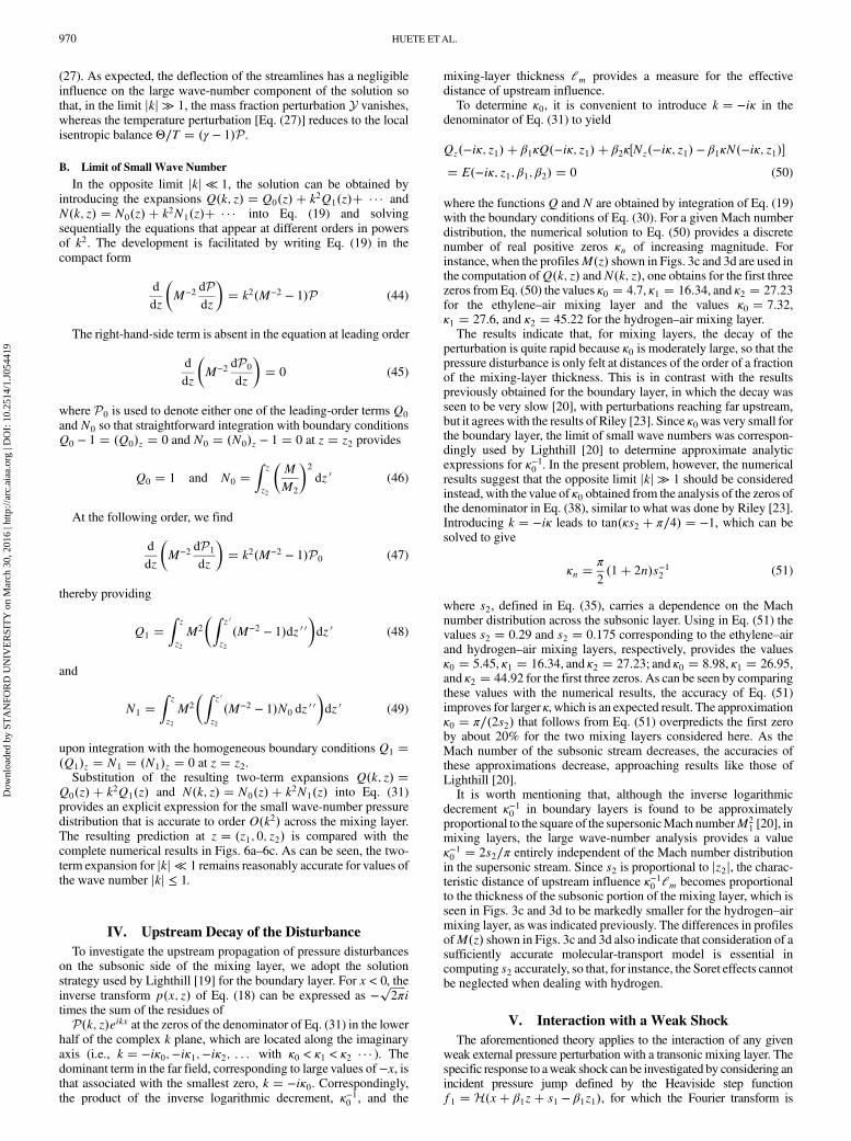
sonic and subsonic domains and the intermediate sonic-line pressuredistribution [Eq. (54)] are represented in Figs. 7a–7f for the ethylene–air andhydrogen–airmixing layers. The trajectories of the incident andreflected waves in the supersonic stream and the distributed pressuredisturbances in the subsonic stream are qualitatively similar for bothmixing layers, although quantitative differences arise from the asso-ciated differences in Mach number distribution displayed in Figs. 2c

a)

e)

c)

b)

f)

d)

Fig. 7 Pressure perturbation from evaluation of Eq. (52) a, b), Eq. (54) c, d), and Eq. (53) e, f), for the ethylene–air (left-hand-side) and hydrogen–air(right-hand-side).

HUETE ETAL. 971

Dow

nloa

ded

by S

TA

NFO

RD

UN

IVE

RSI

TY

on

Mar

ch 3

0, 2

016

| http

://ar

c.ai

aa.o

rg |

DO

I: 1

0.25

14/1

.J05

4419

and 2d. Along the sonic line, however, the streamwise pressure distri-butions are practically indistinguishable because the values of�Mz�0��1∕6 in Eq. (54) happen to be approximately equal for these twoconfigurations. Since, in the limit of jkj ≫ 1 the functionsP andΘ areproportional, as dictated by Eq. (27), the corresponding temperature-perturbation field θ�x; z�would satisfy θ � �γ − 1�Tp, thereby givinga spatial distribution qualitatively similar to that shown in Fig. 6 for thepressure-perturbation field.The logarithmic singularity of the reflected wave and the algebraic

singularity jxj−1∕6 at the point of incidence, both of which also arepresent in the original boundary-layer analysis of Lighthill [19],appear to be inconsistent with the hypothesis of small disturbances.They emerge in the linear theory as a consequence of the discon-tinuous nature of the incident pressure wave. It is naturally expectedthat, in realistic configurations, the singularity would disappear as aconsequence of nonlinear effects acting locally, leading to a pressurefield that would be similar to that depicted in Figs. 7a and 7f, exceptnear the singularities, where the infinities would be replaced by largebut finite values of the pressure. As noted by Lighthill [19] forboundary-layer flows, this view seems to be supported by experi-mental observations [34–37].In the framework of the linear theory, the pressure singularity can

be removed by accounting for the finite thickness of the incidentweak shock: an approach that is motivated by the fact that the shockthickness is inversely proportional to the shock strength [38]. As asimplified example, one may consider external perturbations with apiecewise linear pressure distribution

f1�x; z� ��x��H�x�� − �x� − ls�H�x� − ls�

ls

(57)

where x� � x� β1z� s1 − β1z1 is the incident wave path, and ls isthe ratio of the shock-wave thickness to the mixing-layer thicknesslm. The corresponding Fourier transform

F1�k� ��1 − eikls

k2� lsπδ�k�

�eik�s1−β1z1�

ls

������2π

p (58)

can be used in the large wave-number prediction [Eq. (40)] togenerate from Eq. (18) the pressure distribution

p�x; z� ������β1β

sM

M1

��x� s�H�x� s�− �x� s− ls�H�x� s− ls�ls

�

(59)

if x < s, and

p�x; z� ������β1β

sM

M1

�−~γ � 1

π

−�x − s� ln �x − s� − �x − s − ls� ln�x − s − ls�

πls

�(60)

if x > s, which, unlike Eq. (52), yields a finite value of p along theright-running characteristic x � −s�z�. Similarly, contrary to theircounterparts [Eq. (54) and (55)], the corresponding expressions forthe pressure distribution along the sonic line

p�x; 0� ������β1

p���2

plsM1�Mz�0��1∕6

61∕3�−5∕6�!�����������������2� ���

3pp

5�−1∕3�!

×��2 −

���3

p��jx − lsj5∕6 − jxj5∕6� − jx − lsj5∕6sign�x − ls�

� jxj5∕6sign�x��

(61)

and the associated reflected shock, which follows the pathx− � x� β1z1 − s1 − β1z,

g1�x; z� � −~γ � 1

π−�x−� ln�x−� − �x− − ls� ln�x− − ls�

πls

(62)

are free from singularities, with the infinities in pressure present inEqs. (54) and (55) being replaced by large peak values of order l−1∕6

s

in Eq. (61) and of order ln�l−1s � in Eq. (62). These results indicate that

the singularities of the infinitesimally thin shock translate into a ridgewhen the finite thickness of the shock is considered.

VI. Vorticity Production

Although, unlike the work of Buttsworth [25], only weak shocksare addressed in this study, the results can be used to examine trendsof induced effects in applications involving shock wave ignition offuel–air mixing-layer flows, which are of interest for combustionprocesses in supersonic engines. For example, the direct effects of theincident pressure wave on the fuel and temperature distributions aredescribed by Eq. (26) and (27), giving results that could beincorporated as perturbations in computations of ignition distancesby integration of the flow equations downstream from the interactionregion. The results would be qualitatively indicative of the influencesof stronger shocks.The interaction of the pressure wave leads to an additional indirect

(although possibly important) effect associated with the local genera-tion of vorticity, which may promote the instability of the mixing-layer flow, thereby enhancing the combustion rate by increasing thedownstream mixing rate of the two streams. Alternatively, this effectcould also reduce the vorticity, and thereby inhibit instability and itsassociated turbulent mixing. In examining vorticity production, it isconvenient to express the perturbed nondimensional vorticity, scaledwith its characteristic value U 0

1∕lm, in the form Uz�z� � εω�x; z�.Here, Uz is clearly positive in the mixing layer and corresponds to apositive base-flow vorticity according to the conventional right-handrule, with this being the component of the vorticity vector in thedirection pointing into the paper (positive y direction in Fig. 2). Positivevalues of ω therefore increase the vorticity, and thus presumablyenhance the instabilityof the laminarmixing layers, leading to an earlieronset of turbulence along with increased overall mixing rates.The equation forω � ∂u∕∂z − ∂v∕∂x can be shown from Eq. (12)

to be given by

U∂ω∂x

� vUzz � Uz

�∂u∂x

� ∂v∂z

�−

1

M21

Rz

R2

∂p∂x

(63)

which indicates that, along the perturbed streamline, the vorticitychanges through the combined effects of variable-density flowstretching and baroclinic torque: see the two source terms on theright-hand side of Eq. (63). The former arises as a result of theinteraction of the induced dilatation rate with the background shear,whereas the latter is the result of the nonalignment of the inducedpressure gradient and the background density gradient. The secondterm on the left-hand side of Eq. (63) emerges because of thedeflection of the streamlines, with its magnitude being proportionalto the curvature of the base-flow velocity Uzz.The vorticity equation [Eq. (63)] can be expressed in a more

compact form by using Eq. (1) together with

∂u∂x

� ∂v∂z

� −U∂p∂x

(64)

obtained from a straightforward combination of Eqs. (12a) and (12d)to yield

∂ω∂x

� −Ω∂p∂x

−Uzz

Uv (65)

where the vorticity-production factor

Ω�z� � Uz �U

M2

Rz

R(66)

972 HUETE ETAL.

Dow

nloa

ded

by S

TA

NFO

RD

UN

IVE

RSI

TY

on

Mar

ch 3

0, 2

016

| http

://ar

c.ai

aa.o

rg |

DO

I: 1

0.25

14/1

.J05

4419

measures the collective effects of flow stretching and baroclinictorque. Taking the streamwise derivative of Eq. (65) and expressingthe result in Fourier space, after using Eq. (12c) to eliminate ∂v∕∂x,yields

ϖ � −ΩP −Uzz

Pz

k2M2(67)

for the transform ϖ�k; z� of the vorticity perturbation, defined by itsinverse transform

ω�x; z� � �2π�−1∕2Z

∞

−∞eikxϖ�k; z� dk (68)

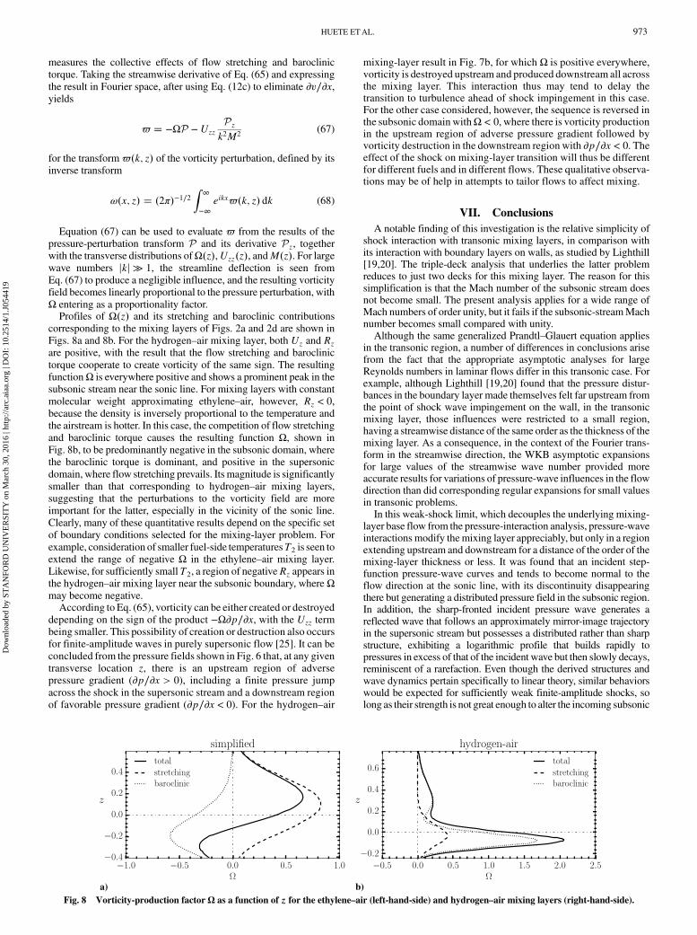
Equation (67) can be used to evaluate ϖ from the results of thepressure-perturbation transform P and its derivative Pz, togetherwith the transverse distributions ofΩ�z�,Uzz�z�, andM�z�. For largewave numbers jkj ≫ 1, the streamline deflection is seen fromEq. (67) to produce a negligible influence, and the resulting vorticityfield becomes linearly proportional to the pressure perturbation, withΩ entering as a proportionality factor.Profiles of Ω�z� and its stretching and baroclinic contributions

corresponding to the mixing layers of Figs. 2a and 2d are shown inFigs. 8a and 8b. For the hydrogen–air mixing layer, both Uz and Rz

are positive, with the result that the flow stretching and baroclinictorque cooperate to create vorticity of the same sign. The resultingfunctionΩ is everywhere positive and shows a prominent peak in thesubsonic stream near the sonic line. For mixing layers with constantmolecular weight approximating ethylene–air, however, Rz < 0,because the density is inversely proportional to the temperature andthe airstream is hotter. In this case, the competition of flow stretchingand baroclinic torque causes the resulting function Ω, shown inFig. 8b, to be predominantly negative in the subsonic domain, wherethe baroclinic torque is dominant, and positive in the supersonicdomain, where flow stretching prevails. Its magnitude is significantlysmaller than that corresponding to hydrogen–air mixing layers,suggesting that the perturbations to the vorticity field are moreimportant for the latter, especially in the vicinity of the sonic line.Clearly, many of these quantitative results depend on the specific setof boundary conditions selected for the mixing-layer problem. Forexample, consideration of smaller fuel-side temperaturesT2 is seen toextend the range of negative Ω in the ethylene–air mixing layer.Likewise, for sufficiently small T2, a region of negativeRz appears inthe hydrogen–air mixing layer near the subsonic boundary, where Ωmay become negative.According to Eq. (65), vorticity can be either created or destroyed

depending on the sign of the product −Ω∂p∕∂x, with the Uzz termbeing smaller. This possibility of creation or destruction also occursfor finite-amplitude waves in purely supersonic flow [25]. It can beconcluded from the pressure fields shown in Fig. 6 that, at any giventransverse location z, there is an upstream region of adversepressure gradient (∂p∕∂x > 0), including a finite pressure jumpacross the shock in the supersonic stream and a downstream regionof favorable pressure gradient (∂p∕∂x < 0). For the hydrogen–air

mixing-layer result in Fig. 7b, for which Ω is positive everywhere,vorticity is destroyed upstream and produced downstream all acrossthe mixing layer. This interaction thus may tend to delay thetransition to turbulence ahead of shock impingement in this case.For the other case considered, however, the sequence is reversed inthe subsonic domain withΩ < 0, where there is vorticity productionin the upstream region of adverse pressure gradient followed byvorticity destruction in the downstream region with ∂p∕∂x < 0. Theeffect of the shock on mixing-layer transition will thus be differentfor different fuels and in different flows. These qualitative observa-tions may be of help in attempts to tailor flows to affect mixing.

VII. Conclusions

A notable finding of this investigation is the relative simplicity ofshock interaction with transonic mixing layers, in comparison withits interaction with boundary layers on walls, as studied by Lighthill[19,20]. The triple-deck analysis that underlies the latter problemreduces to just two decks for this mixing layer. The reason for thissimplification is that the Mach number of the subsonic stream doesnot become small. The present analysis applies for a wide range ofMach numbers of order unity, but it fails if the subsonic-streamMachnumber becomes small compared with unity.Although the same generalized Prandtl–Glauert equation applies

in the transonic region, a number of differences in conclusions arisefrom the fact that the appropriate asymptotic analyses for largeReynolds numbers in laminar flows differ in this transonic case. Forexample, although Lighthill [19,20] found that the pressure distur-bances in the boundary layer made themselves felt far upstream fromthe point of shock wave impingement on the wall, in the transonicmixing layer, those influences were restricted to a small region,having a streamwise distance of the same order as the thickness of themixing layer. As a consequence, in the context of the Fourier trans-form in the streamwise direction, the WKB asymptotic expansionsfor large values of the streamwise wave number provided moreaccurate results for variations of pressure-wave influences in the flowdirection than did corresponding regular expansions for small valuesin transonic problems.In this weak-shock limit, which decouples the underlying mixing-

layer base flow from the pressure-interaction analysis, pressure-waveinteractions modify themixing layer appreciably, but only in a regionextending upstream and downstream for a distance of the order of themixing-layer thickness or less. It was found that an incident step-function pressure-wave curves and tends to become normal to theflow direction at the sonic line, with its discontinuity disappearingthere but generating a distributed pressure field in the subsonic region.In addition, the sharp-fronted incident pressure wave generates areflected wave that follows an approximately mirror-image trajectoryin the supersonic stream but possesses a distributed rather than sharpstructure, exhibiting a logarithmic profile that builds rapidly topressures in excess of that of the incident wave but then slowly decays,reminiscent of a rarefaction. Even though the derived structures andwave dynamics pertain specifically to linear theory, similar behaviorswould be expected for sufficiently weak finite-amplitude shocks, solong as their strength is not great enough to alter the incoming subsonic

a) b)Fig. 8 Vorticity-production factor Ω as a function of z for the ethylene–air (left-hand-side) and hydrogen–air mixing layers (right-hand-side).

HUETE ETAL. 973

Dow

nloa

ded

by S

TA

NFO

RD

UN

IVE

RSI

TY

on

Mar

ch 3

0, 2

016

| http

://ar

c.ai

aa.o

rg |

DO

I: 1

0.25

14/1

.J05

4419

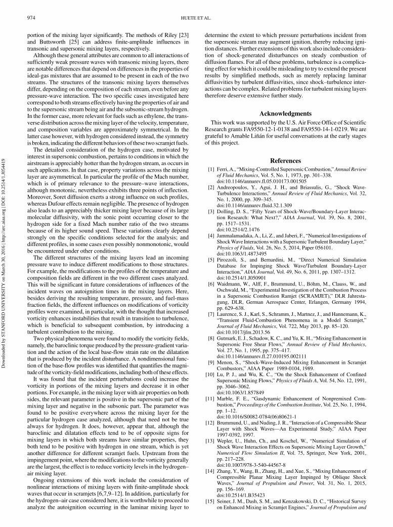
portion of the mixing layer significantly. The methods of Riley [23]and Buttsworth [25] can address finite-amplitude influences intransonic and supersonic mixing layers, respectively.Although these general attributes are common to all interactions of

sufficiently weak pressure waves with transonic mixing layers, thereare notable differences that depend on differences in the properties ofideal-gas mixtures that are assumed to be present in each of the twostreams. The structures of the transonic mixing layers themselvesdiffer, depending on the composition of each stream, even before anypressure-wave interaction. The two specific cases investigated herecorrespond to both streams effectively having the properties of air andto the supersonic stream being air and the subsonic-stream hydrogen.In the former case, more relevant for fuels such as ethylene, the trans-verse distribution across themixing layer of thevelocity, temperature,and composition variables are approximately symmetrical. In thelatter case however, with hydrogen considered instead, the symmetryisbroken, indicating the different behaviors of these two scramjet fuels.The detailed consideration of the hydrogen case, motivated by

interest in supersonic combustion, pertains to conditions in which theairstream is appreciably hotter than the hydrogen stream, as occurs insuch applications. In that case, property variations across the mixinglayer are asymmetrical. In particular the profile of the Mach number,which is of primary relevance to the pressure–wave interactions,although monotonic, nevertheless exhibits three points of inflection.Moreover, Soret diffusion exerts a strong influence on such profiles,whereas Dufour effects remain negligible. The presence of hydrogenalso leads to an appreciably thicker mixing layer because of its largemolecular diffusivity, with the sonic point occurring closer to thehydrogen side for a fixed Mach number ratio of the two streamsbecause of its higher sound speed. These variations clearly dependstrongly on the specific conditions selected for the analysis; anddifferent profiles, in some cases even possibly nonmonotonic, wouldbe encountered under other conditions.The different structures of the mixing layers lead an incoming

pressure wave to induce different modifications to those structures.For example, the modifications to the profiles of the temperature andcomposition fields are different in the two different cases analyzed.This will be significant in future considerations of influences of theincident waves on autoignition times in the mixing layers. Here,besides deriving the resulting temperature, pressure, and fuel-massfraction fields, the different influences on modifications of vorticityprofiles were examined, in particular, with the thought that increasedvorticity enhances instabilities that result in transition to turbulence,which is beneficial to subsequent combustion, by introducing aturbulent contribution to the mixing.Two physical phenomena were found to modify the vorticity fields,

namely, the baroclinic torque produced by the pressure-gradient varia-tion and the action of the local base-flow strain rate on the dilatationthat is produced by the incident disturbance. A nondimensional func-tion of the base-flow profiles was identified that quantifies the magni-tudeof thevorticity-fieldmodifications, includingbothof these effects.It was found that the incident perturbations could increase the

vorticity in portions of the mixing layers and decrease it in otherportions. For example, in the mixing layer with air properties on bothsides, the relevant parameter is positive in the supersonic part of themixing layer and negative in the subsonic part. The parameter wasfound to be positive everywhere across the mixing layer for theparticular hydrogen case analyzed, although that need not be truealways for hydrogen. It does, however, appear that, although thebaroclinic and dilatation effects tend to be of opposite signs formixing layers in which both streams have similar properties, theyboth tend to be positive with hydrogen in one stream, which is yetanother difference for different scramjet fuels. Upstream from theimpingement point, where themodifications to the vorticity generallyare the largest, the effect is to reduce vorticity levels in the hydrogen–air mixing layer.Ongoing extensions of this work include the consideration of

nonlinear interactions of mixing layers with finite-amplitude shockwaves that occur in scramjets [6,7,9–12]. In addition, particularly forthe hydrogen–air case considered here, it is worthwhile to proceed toanalyze the autoignition occurring in the laminar mixing layer to

determine the extent to which pressure perturbations incident fromthe supersonic stream may augment ignition, thereby reducing igni-tion distances. Further extensions of thiswork also include considera-tion of shock-generated disturbances on steady combustion ofdiffusion flames. For all of these problems, turbulence is a complica-ting effect for which it could bemisleading to try to extend the presentresults by simplified methods, such as merely replacing laminardiffusivities by turbulent diffusivities, since shock–turbulence inter-actions can be complex. Related problems for turbulentmixing layerstherefore deserve extensive further study.

Acknowledgments

This work was supported by the U.S. Air ForceOffice of ScientificResearch grants FA9550-12-1-0138 and FA9550-14-1-0219. We aregrateful to Amable Liñán for useful conversations at the early stagesof this project.

References

[1] Ferri, A., “Mixing-Controlled Supersonic Combustion,”Annual Reviewof Fluid Mechanics, Vol. 5, No. 1, 1973, pp. 301–338.doi:10.1146/annurev.fl.05.010173.001505

[2] Andreopoulos, Y., Agui, J. H., and Briassulis, G., “Shock Wave-Turbulence Interactions,” Annual Review of Fluid Mechanics, Vol. 32,No. 1, 2000, pp. 309–345.doi:10.1146/annurev.fluid.32.1.309

[3] Dolling, D. S., “Fifty Years of Shock-Wave/Boundary-Layer Interac-tion Research: What Next?,” AIAA Journal, Vol. 39, No. 8, 2001,pp. 1517–1531.doi:10.2514/2.1476

[4] Jammalamadaka, A., Li, Z., and Jaberi, F., “Numerical Investigations ofShockWave Interactionswith a Supersonic Turbulent BoundaryLayer,”Physics of Fluids, Vol. 26, No. 5, 2014, Paper 056101.doi:10.1063/1.4873495

[5] Pirozzoli, S., and Bernardini, M., “Direct Numerical SimulationDatabase for Impinging Shock Wave/Turbulent Boundary-LayerInteraction,” AIAA Journal, Vol. 49, No. 6, 2011, pp. 1307–1312.doi:10.2514/1.J050901

[6] Waidmann, W., Alff, F., Brummund, U., Böhm, M., Clauss, W., andOschwald, M., “Experimental Investigation of the Combustion Processin a Supersonic Combustion Ramjet (SCRAMJET),” DLR Jahresta-gung, DLR, German Aerospace Center, Erlangen, Germany 1994,pp. 629–638.

[7] Laurence, S. J., Karl, S., Schramm, J., Martnez, J., and Hannemann, K.,“Transient Fluid-Combustion Phenomena in a Model Scramjet,”Journal of Fluid Mechanics, Vol. 722, May 2013, pp. 85–120.doi:10.1017/jfm.2013.56

[8] Gutmark, E. J., Schadow,K. C., andYu, K.H., “MixingEnhancement inSupersonic Free Shear Flows,” Annual Review of Fluid Mechanics,Vol. 27, No. 1, 1995, pp. 375–417.doi:10.1146/annurev.fl.27.010195.002111

[9] Menon, S., “Shock-Wave-Induced Mixing Enhancement in ScramjetCombustors,” AIAA Paper 1989-0104, 1989.

[10] Lu, P. J., and Wu, K. C., “On the Shock Enhancement of ConfinedSupersonic Mixing Flows,” Physics of Fluids A, Vol. 54, No. 12, 1991,pp. 3046–3062.doi:10.1063/1.857849

[11] Marble, F. E., “Gasdynamic Enhancement of Nonpremixed Com-bustion,” Proceedings of the Combustion Institute, Vol. 25, No. 1, 1994,pp. 1–12.doi:10.1016/S0082-0784(06)80621-1

[12] Brummund, U., andNuding, J. R., “Interaction of a Compressible ShearLayer with Shock Waves—An Experimental Study,” AIAA Paper1997-0392, 1997.

[13] Wepler, U., Huhn, Ch., and Koschel, W., “Numerical Simulation ofShock Wave Interaction Effects on Supersonic Mixing Layer Growth,”Numerical Flow Simulation II, Vol. 75, Springer, New York, 2001,pp. 217–228.doi:10.1007/978-3-540-44567-8

[14] Zhang, Y., Wang, B., Zhang, H., and Xue, S., “Mixing Enhancement ofCompressible Planar Mixing Layer Impinged by Oblique ShockWaves,” Journal of Propulsion and Power, Vol. 31, No. 1, 2015,pp. 156–169.doi:10.2514/1.B35423

[15] Seiner, J. M., Dash, S. M., and Kenzakowski, D. C., “Historical Surveyon Enhanced Mixing in Scramjet Engines,” Journal of Propulsion and

974 HUETE ETAL.

Dow

nloa

ded

by S

TA

NFO

RD

UN

IVE

RSI

TY

on

Mar

ch 3

0, 2

016

| http

://ar

c.ai

aa.o

rg |

DO

I: 1

0.25

14/1

.J05

4419

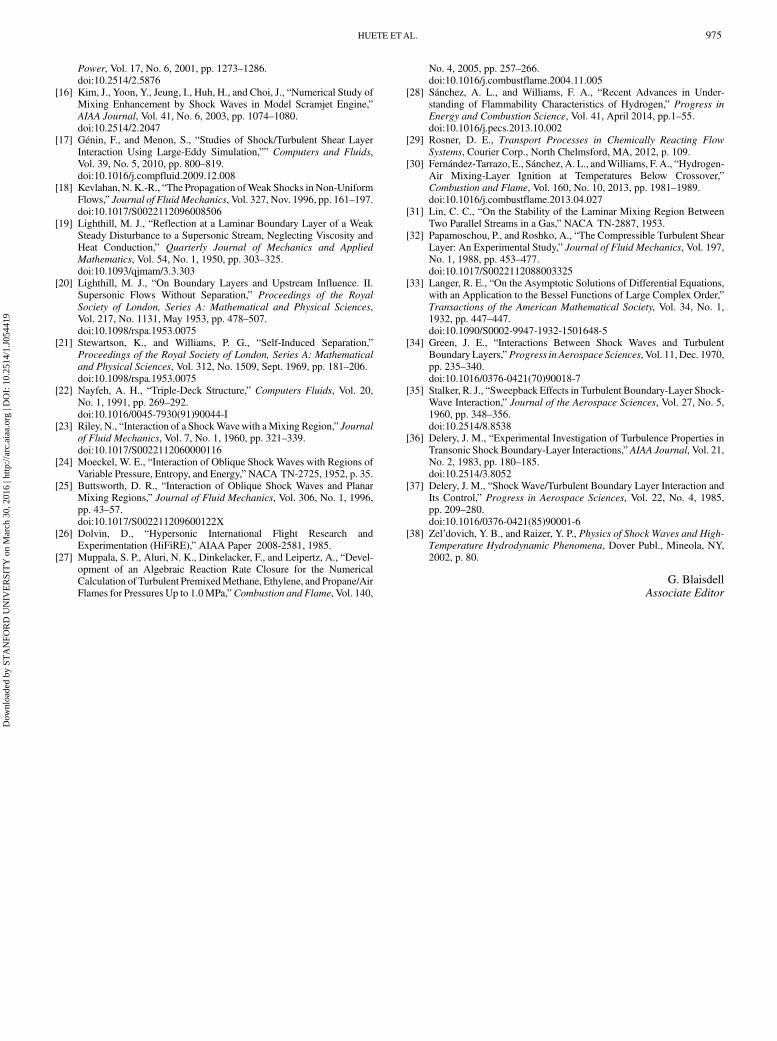
Power, Vol. 17, No. 6, 2001, pp. 1273–1286.doi:10.2514/2.5876

[16] Kim, J., Yoon, Y., Jeung, I., Huh, H., and Choi, J., “Numerical Study ofMixing Enhancement by Shock Waves in Model Scramjet Engine,”AIAA Journal, Vol. 41, No. 6, 2003, pp. 1074–1080.doi:10.2514/2.2047

[17] Génin, F., and Menon, S., “Studies of Shock/Turbulent Shear LayerInteraction Using Large-Eddy Simulation,”” Computers and Fluids,Vol. 39, No. 5, 2010, pp. 800–819.doi:10.1016/j.compfluid.2009.12.008

[18] Kevlahan, N. K.-R., “The Propagation ofWeak Shocks in Non-UniformFlows,” Journal of FluidMechanics, Vol. 327, Nov. 1996, pp. 161–197.doi:10.1017/S0022112096008506

[19] Lighthill, M. J., “Reflection at a Laminar Boundary Layer of a WeakSteady Disturbance to a Supersonic Stream, Neglecting Viscosity andHeat Conduction,” Quarterly Journal of Mechanics and Applied

Mathematics, Vol. 54, No. 1, 1950, pp. 303–325.doi:10.1093/qjmam/3.3.303

[20] Lighthill, M. J., “On Boundary Layers and Upstream Influence. II.Supersonic Flows Without Separation,” Proceedings of the Royal

Society of London, Series A: Mathematical and Physical Sciences,Vol. 217, No. 1131, May 1953, pp. 478–507.doi:10.1098/rspa.1953.0075

[21] Stewartson, K., and Williams, P. G., “Self-Induced Separation,”Proceedings of the Royal Society of London, Series A: Mathematical

and Physical Sciences, Vol. 312, No. 1509, Sept. 1969, pp. 181–206.doi:10.1098/rspa.1953.0075

[22] Nayfeh, A. H., “Triple-Deck Structure,” Computers Fluids, Vol. 20,No. 1, 1991, pp. 269–292.doi:10.1016/0045-7930(91)90044-I

[23] Riley, N., “Interaction of a ShockWavewith aMixing Region,” Journalof Fluid Mechanics, Vol. 7, No. 1, 1960, pp. 321–339.doi:10.1017/S0022112060000116

[24] Moeckel, W. E., “Interaction of Oblique Shock Waves with Regions ofVariable Pressure, Entropy, and Energy,”NACA TN-2725, 1952, p. 35.

[25] Buttsworth, D. R., “Interaction of Oblique Shock Waves and PlanarMixing Regions,” Journal of Fluid Mechanics, Vol. 306, No. 1, 1996,pp. 43–57.doi:10.1017/S002211209600122X

[26] Dolvin, D., “Hypersonic International Flight Research andExperimentation (HiFiRE),” AIAA Paper 2008-2581, 1985.

[27] Muppala, S. P., Aluri, N. K., Dinkelacker, F., and Leipertz, A., “Devel-opment of an Algebraic Reaction Rate Closure for the NumericalCalculation of Turbulent PremixedMethane, Ethylene, and Propane/AirFlames for Pressures Up to 1.0MPa,”Combustion and Flame, Vol. 140,

No. 4, 2005, pp. 257–266.doi:10.1016/j.combustflame.2004.11.005

[28] Sánchez, A. L., and Williams, F. A., “Recent Advances in Under-standing of Flammability Characteristics of Hydrogen,” Progress in

Energy and Combustion Science, Vol. 41, April 2014, pp.1–55.doi:10.1016/j.pecs.2013.10.002

[29] Rosner, D. E., Transport Processes in Chemically Reacting Flow

Systems, Courier Corp., North Chelmsford, MA, 2012, p. 109.[30] Fernández-Tarrazo, E., Sánchez, A. L., andWilliams, F. A., “Hydrogen-

Air Mixing-Layer Ignition at Temperatures Below Crossover,”Combustion and Flame, Vol. 160, No. 10, 2013, pp. 1981–1989.doi:10.1016/j.combustflame.2013.04.027

[31] Lin, C. C., “On the Stability of the Laminar Mixing Region BetweenTwo Parallel Streams in a Gas,” NACA TN-2887, 1953.

[32] Papamoschou, P., and Roshko, A., “The Compressible Turbulent ShearLayer: An Experimental Study,” Journal of Fluid Mechanics, Vol. 197,No. 1, 1988, pp. 453–477.doi:10.1017/S0022112088003325

[33] Langer, R. E., “On the Asymptotic Solutions of Differential Equations,with an Application to the Bessel Functions of Large Complex Order,”Transactions of the American Mathematical Society, Vol. 34, No. 1,1932, pp. 447–447.doi:10.1090/S0002-9947-1932-1501648-5

[34] Green, J. E., “Interactions Between Shock Waves and TurbulentBoundary Layers,”Progress in Aerospace Sciences, Vol. 11, Dec. 1970,pp. 235–340.doi:10.1016/0376-0421(70)90018-7

[35] Stalker, R. J., “Sweepback Effects in Turbulent Boundary-Layer Shock-Wave Interaction,” Journal of the Aerospace Sciences, Vol. 27, No. 5,1960, pp. 348–356.doi:10.2514/8.8538

[36] Delery, J. M., “Experimental Investigation of Turbulence Properties inTransonic Shock Boundary-Layer Interactions,” AIAA Journal, Vol. 21,No. 2, 1983, pp. 180–185.doi:10.2514/3.8052

[37] Delery, J. M., “Shock Wave/Turbulent Boundary Layer Interaction andIts Control,” Progress in Aerospace Sciences, Vol. 22, No. 4, 1985,pp. 209–280.doi:10.1016/0376-0421(85)90001-6

[38] Zel’dovich, Y. B., and Raizer, Y. P., Physics of Shock Waves and High-

Temperature Hydrodynamic Phenomena, Dover Publ., Mineola, NY,2002, p. 80.

G. BlaisdellAssociate Editor

HUETE ETAL. 975

Dow

nloa

ded

by S

TA

NFO

RD

UN

IVE

RSI

TY

on

Mar

ch 3

0, 2

016

| http

://ar

c.ai

aa.o

rg |

DO

I: 1

0.25

14/1

.J05

4419