Wavelet Applications - umu.se · Wavelet Applications 1-3 Wavelet Applications Wavelets have scale...

Wavelet Applications

1-3

Wavelet ApplicationsWavelets have scale aspects and time aspects, consequently every application has scale and time aspects. To clarify them we try to untangle the aspects somewhat arbitrarily.

For scale aspects, we present one idea around the notion of local regularity. For time aspects, we present a list of domains. When the decomposition is taken as a whole, the de-noising and compression processes are center points.

Scale aspectsAs a complement to the spectral signal analysis, new signal forms appear. They are less regular signals than the usual ones.

The cusp signal presents a very quick local variation. Its equation is with t close to 0 and 0 < r < 1. The lower r the sharper the signal.

To illustrate this notion physically, imagine you take a piece of aluminum foil; The surface is very smooth, very regular. You first crush it into a ball, and then you spread it out so that it looks like a surface. The asperities are clearly visible. Each one represents a two-dimension cusp and analog of the one dimensional cusp. If you crush again the foil, more tightly, in a more compact ball, when you spread it out, the roughness increases and the regularity decreases.

Several domains use the wavelet techniques of regularity study:

• Biology for cell membrane recognition, to distinguish the normal from the pathological membranes

• Metallurgy for the characterization of rough surfaces

• Finance (which is more surprising), for detecting the properties of quick variation of values

• In Internet traffic description, for designing the services size

Time aspectsLet’s switch to time aspects. The main goals are:

• Rupture and edges detection

• Study of short-time phenomena as transient processes

tr

1 Wavelets: A New Tool for Signal Analysis

1-4

As domain applications, we get:

• Industrial supervision of gear-wheel

• Checking undue noises in craned or dented wheels, and more generally in non destructive control quality processes

• Detection of short pathological events as epileptic crises or normal ones as evoked potentials in EEG (medicine)

• SAR imagery

• Automatic target recognition

• Intermittence in physics

Wavelet Decomposition as a WholeMany applications use the wavelet decomposition taken as a whole. The common goals concern the signal or image clearance and simplification, which are parts of de-noising or compression.

We find many published papers in oceanography and earth studies.

One of the most popular successes of the wavelets is the compression of the FBI fingerprints.

When trying to classify the applications by domain, it is almost impossible to sum up several thousand papers written within the last 15 years. Moreover, it is difficult to get information on real-world industrial applications from companies. They understandably protect their own information.

Some domains are very productive. Medicine is one of them. We can find studies on micro-potential extraction in EKGs, on time localization of His bundle electrical heart activity, in ECG noise removal. In EEGs, a quick transitory signal is drowned in the usual one. The wavelets are able to determine if a quick signal exists, and if so, can localize it. There are attempts to enhance mammograms to discriminate tumors from calcifications.

Another prototypical application is a classification of Magnetic Resonance Spectra. The study concerns the influence of the fat we eat on our body fat. The type of feeding is the basic information and the study is intended to avoid taking a sample of the body fat. Each Fourier spectrum is encoded by some of its wavelet coefficients. A few of them are enough to code the most interesting features of the spectrum. The classification is performed on the coded vectors.

Fourier Analysis

1-5

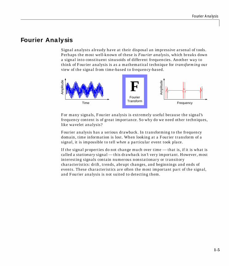
Fourier AnalysisSignal analysts already have at their disposal an impressive arsenal of tools. Perhaps the most well-known of these is Fourier analysis, which breaks down a signal into constituent sinusoids of different frequencies. Another way to think of Fourier analysis is as a mathematical technique for transforming our view of the signal from time-based to frequency-based.

For many signals, Fourier analysis is extremely useful because the signal’s frequency content is of great importance. So why do we need other techniques, like wavelet analysis?

Fourier analysis has a serious drawback. In transforming to the frequency domain, time information is lost. When looking at a Fourier transform of a signal, it is impossible to tell when a particular event took place.

If the signal properties do not change much over time — that is, if it is what is called a stationary signal — this drawback isn’t very important. However, most interesting signals contain numerous nonstationary or transitory characteristics: drift, trends, abrupt changes, and beginnings and ends of events. These characteristics are often the most important part of the signal, and Fourier analysis is not suited to detecting them.

FFourier

Transform

Am

plitu

de

Time

Am

plitu

de

Frequency


1-6

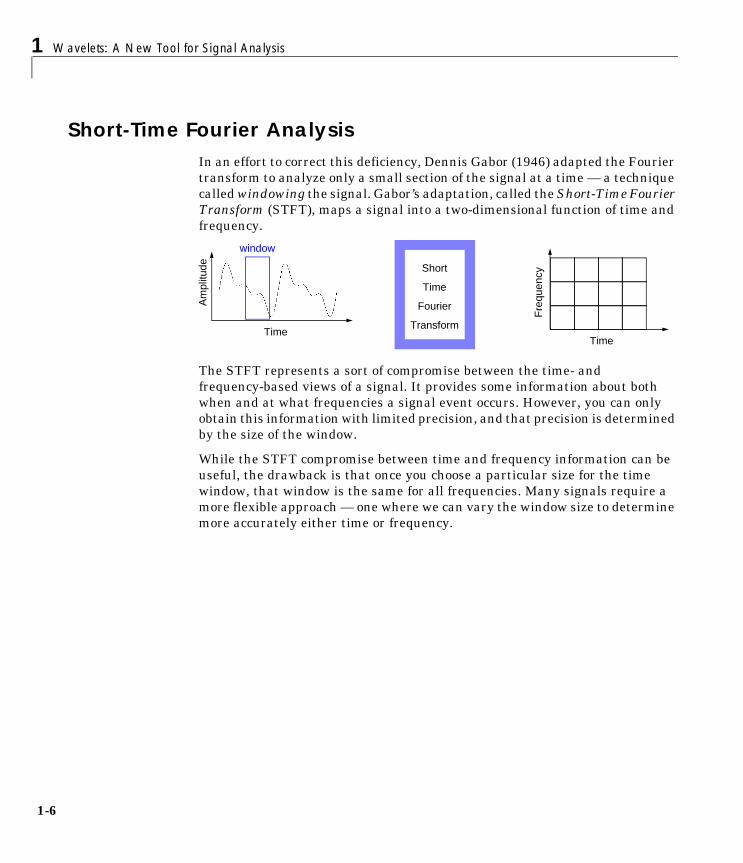
Short-Time Fourier AnalysisIn an effort to correct this deficiency, Dennis Gabor (1946) adapted the Fourier transform to analyze only a small section of the signal at a time — a technique called windowing the signal. Gabor’s adaptation, called the Short-Time Fourier Transform (STFT), maps a signal into a two-dimensional function of time and frequency.

The STFT represents a sort of compromise between the time- and frequency-based views of a signal. It provides some information about both when and at what frequencies a signal event occurs. However, you can only obtain this information with limited precision, and that precision is determined by the size of the window.

While the STFT compromise between time and frequency information can be useful, the drawback is that once you choose a particular size for the time window, that window is the same for all frequencies. Many signals require a more flexible approach — one where we can vary the window size to determine more accurately either time or frequency.

Short

Transform

Am

plitu

de

TimeTime

Time

Fourier

Fre

quen

cy

window

Wavelet Analysis

1-7

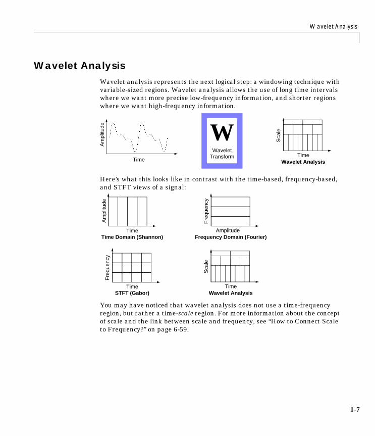
Wavelet AnalysisWavelet analysis represents the next logical step: a windowing technique with variable-sized regions. Wavelet analysis allows the use of long time intervals where we want more precise low-frequency information, and shorter regions where we want high-frequency information.

Here’s what this looks like in contrast with the time-based, frequency-based, and STFT views of a signal:

You may have noticed that wavelet analysis does not use a time-frequency region, but rather a time-scale region. For more information about the concept of scale and the link between scale and frequency, see “How to Connect Scale to Frequency?” on page 6-59.

Am

plitu

de

TimeTime

Sca

le

Wavelet Analysis

WWavelet

Transform

Time

Fre

quen

cy

Time

Sca

le

STFT (Gabor) Wavelet Analysis

TimeTime Domain (Shannon)

Fre

quen

cy

Frequency Domain (Fourier)Amplitude

Am

plitu

de


1-8

What Can Wavelet Analysis Do?One major advantage afforded by wavelets is the ability to perform local analysis — that is, to analyze a localized area of a larger signal.

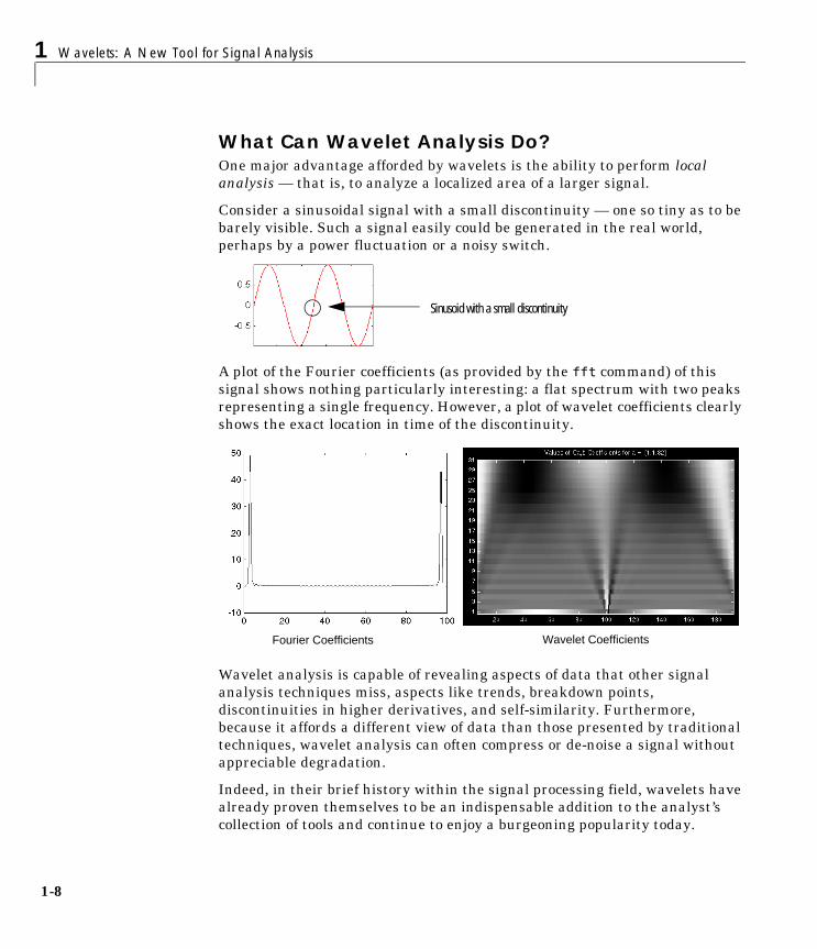
Consider a sinusoidal signal with a small discontinuity — one so tiny as to be barely visible. Such a signal easily could be generated in the real world, perhaps by a power fluctuation or a noisy switch.

A plot of the Fourier coefficients (as provided by the fft command) of this signal shows nothing particularly interesting: a flat spectrum with two peaks representing a single frequency. However, a plot of wavelet coefficients clearly shows the exact location in time of the discontinuity.

Wavelet analysis is capable of revealing aspects of data that other signal analysis techniques miss, aspects like trends, breakdown points, discontinuities in higher derivatives, and self-similarity. Furthermore, because it affords a different view of data than those presented by traditional techniques, wavelet analysis can often compress or de-noise a signal without appreciable degradation.

Indeed, in their brief history within the signal processing field, wavelets have already proven themselves to be an indispensable addition to the analyst’s collection of tools and continue to enjoy a burgeoning popularity today.

Sinusoid with a small discontinuity

Fourier Coefficients Wavelet Coefficients

What Is Wavelet Analysis?

1-9

What Is Wavelet Analysis?Now that we know some situations when wavelet analysis is useful, it is worthwhile asking “What is wavelet analysis?” and even more fundamentally, “What is a wavelet?”

A wavelet is a waveform of effectively limited duration that has an average value of zero.

Compare wavelets with sine waves, which are the basis of Fourier analysis. Sinusoids do not have limited duration — they extend from minus to plus infinity. And where sinusoids are smooth and predictable, wavelets tend to be irregular and asymmetric.

Fourier analysis consists of breaking up a signal into sine waves of various frequencies. Similarly, wavelet analysis is the breaking up of a signal into shifted and scaled versions of the original (or mother) wavelet.

Just looking at pictures of wavelets and sine waves, you can see intuitively that signals with sharp changes might be better analyzed with an irregular wavelet than with a smooth sinusoid, just as some foods are better handled with a fork than a spoon.

It also makes sense that local features can be described better with wavelets that have local extent.

Number of DimensionsThus far, we’ve discussed only one-dimensional data, which encompasses most ordinary signals. However, wavelet analysis can be applied to two-dimensional data (images) and, in principle, to higher dimensional data.

This toolbox uses only one- and two-dimensional analysis techniques.

Sine Wave Wavelet (db10)

......


1-10

The Continuous Wavelet TransformMathematically, the process of Fourier analysis is represented by the Fourier transform:

which is the sum over all time of the signal f(t) multiplied by a complex exponential. (Recall that a complex exponential can be broken down into real and imaginary sinusoidal components.)

The results of the transform are the Fourier coefficients , which when multiplied by a sinusoid of frequency , yield the constituent sinusoidal components of the original signal. Graphically, the process looks like:

Similarly, the continuous wavelet transform (CWT) is defined as the sum over all time of the signal multiplied by scaled, shifted versions of the wavelet function :

The result of the CWT are many wavelet coefficients C, which are a function of scale and position.

F ω( ) f t( )e jωt–

∞–

∞

∫ dt=

F ω( )ω

Signal

...

Constituent sinusoids of different frequencies

Fourier

Transform

ψ

C scale position,( ) f t( )ψ scale position t,,( ) td∞–

∞

∫=

The Continuous Wavelet Transform

1-11

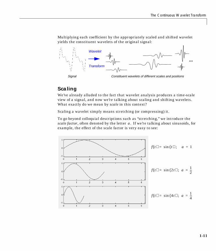
Multiplying each coefficient by the appropriately scaled and shifted wavelet yields the constituent wavelets of the original signal:

ScalingWe’ve already alluded to the fact that wavelet analysis produces a time-scale view of a signal, and now we’re talking about scaling and shifting wavelets. What exactly do we mean by scale in this context?

Scaling a wavelet simply means stretching (or compressing) it.

To go beyond colloquial descriptions such as “stretching,” we introduce the scale factor, often denoted by the letter If we’re talking about sinusoids, for example, the effect of the scale factor is very easy to see:

Signal Constituent wavelets of different scales and positions

...

Wavelet

Transform

a.

f t( ) t( )sin=

f t( ) 2t( )sin=

f t( ) 4t( )sin=

a; 1=

; a 12---=

; a 14---=


1-12

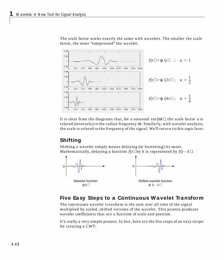
The scale factor works exactly the same with wavelets. The smaller the scale factor, the more “compressed” the wavelet.

It is clear from the diagrams that, for a sinusoid , the scale factor is related (inversely) to the radian frequency . Similarly, with wavelet analysis, the scale is related to the frequency of the signal. We’ll return to this topic later.

ShiftingShifting a wavelet simply means delaying (or hastening) its onset. Mathematically, delaying a function by k is represented by :

Five Easy Steps to a Continuous Wavelet TransformThe continuous wavelet transform is the sum over all time of the signal multiplied by scaled, shifted versions of the wavelet. This process produces wavelet coefficients that are a function of scale and position.

It’s really a very simple process. In fact, here are the five steps of an easy recipe for creating a CWT:

f t( ) ψ t( )=

f t( ) ψ 2t( )=

f t( ) ψ 4t( )=

; a 1=

; a 12---=

; a 14---=

ωt( )sin aω

f t( ) f t k–( )

Wavelet functionψ t( ) ψ t k–( )

Shifted wavelet function

0 0


1-13

1 Take a wavelet and compare it to a section at the start of the original signal.

2 Calculate a number, C, that represents how closely correlated the wavelet is with this section of the signal. The higher C is, the more the similarity. More precisely, if the signal energy and the wavelet energy are equal to one, C may be interpreted as a correlation coefficient.

Note that the results will depend on the shape of the wavelet you choose.

3 Shift the wavelet to the right and repeat steps 1 and 2 until you’ve covered the whole signal.

4 Scale (stretch) the wavelet and repeat steps 1 through 3.

5 Repeat steps 1 through 4 for all scales.

Signal

Wavelet

C = 0.0102

Signal

Wavelet

Signal

Wavelet

C = 0.2247


1-14

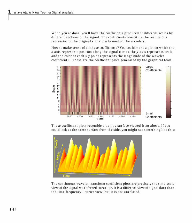
When you’re done, you’ll have the coefficients produced at different scales by different sections of the signal. The coefficients constitute the results of a regression of the original signal performed on the wavelets.

How to make sense of all these coefficients? You could make a plot on which the x-axis represents position along the signal (time), the y-axis represents scale, and the color at each x-y point represents the magnitude of the wavelet coefficient C. These are the coefficient plots generated by the graphical tools.

These coefficient plots resemble a bumpy surface viewed from above. If you could look at the same surface from the side, you might see something like this:

The continuous wavelet transform coefficient plots are precisely the time-scale view of the signal we referred to earlier. It is a different view of signal data than the time-frequency Fourier view, but it is not unrelated.

LargeCoefficients

SmallCoefficients

Sca

le

Time

Time

Sca

leC

oef

s


1-15

Scale and FrequencyNotice that the scales in the coefficients plot (shown as y-axis labels) run from 1 to 31. Recall that the higher scales correspond to the most “stretched” wavelets. The more stretched the wavelet, the longer the portion of the signal with which it is being compared, and thus the coarser the signal features being measured by the wavelet coefficients.

Thus, there is a correspondence between wavelet scales and frequency as revealed by wavelet analysis:

• Low scale a ⇒ Compressed wavelet ⇒ Rapidly changing details ⇒ High frequency .

• High scale a ⇒ Stretched wavelet ⇒ Slowly changing, coarse features ⇒ Low frequency .

The Scale of NatureIt’s important to understand that the fact that wavelet analysis does not produce a time-frequency view of a signal is not a weakness, but a strength of the technique.

Not only is time-scale a different way to view data, it is a very natural way to view data deriving from a great number of natural phenomena.

Signal

Wavelet

Low scale High scale

ω

ω


1-16

Consider a lunar landscape, whose ragged surface (simulated below) is a result of centuries of bombardment by meteorites whose sizes range from gigantic boulders to dust specks.

If we think of this surface in cross-section as a one-dimensional signal, then it is reasonable to think of the signal as having components of different scales — large features carved by the impacts of large meteorites, and finer features abraded by small meteorites.

Here is a case where thinking in terms of scale makes much more sense than thinking in terms of frequency. Inspection of the CWT coefficients plot for this signal reveals patterns among scales and shows the signal’s possibly fractal nature.

Even though this signal is artificial, many natural phenomena — from the intricate branching of blood vessels and trees, to the jagged surfaces of mountains and fractured metals — lend themselves to an analysis of scale.


1-17

What’s Continuous About the Continuous Wavelet Transform?Any signal processing performed on a computer using real-world data must be performed on a discrete signal — that is, on a signal that has been measured at discrete time. So what exactly is “continuous” about it?

What’s “continuous” about the CWT, and what distinguishes it from the discrete wavelet transform (to be discussed in the following section), is the set of scales and positions at which it operates.

Unlike the discrete wavelet transform, the CWT can operate at every scale, from that of the original signal up to some maximum scale that you determine by trading off your need for detailed analysis with available computational horsepower.

The CWT is also continuous in terms of shifting: during computation, the analyzing wavelet is shifted smoothly over the full domain of the analyzed function.


1-18

The Discrete Wavelet TransformCalculating wavelet coefficients at every possible scale is a fair amount of work, and it generates an awful lot of data. What if we choose only a subset of scales and positions at which to make our calculations?

It turns out, rather remarkably, that if we choose scales and positions based on powers of two — so-called dyadic scales and positions — then our analysis will be much more efficient and just as accurate. We obtain such an analysis from the discrete wavelet transform (DWT).

An efficient way to implement this scheme using filters was developed in 1988 by Mallat (see [Mal89] in “References” on page 6-145). The Mallat algorithm is in fact a classical scheme known in the signal processing community as a two-channel subband coder (see page 1 of the book Wavelets and Filter Banks, by Strang and Nguyen [StrN96]).

This very practical filtering algorithm yields a fast wavelet transform — a box into which a signal passes, and out of which wavelet coefficients quickly emerge. Let’s examine this in more depth.

One-Stage Filtering: Approximations and DetailsFor many signals, the low-frequency content is the most important part. It is what gives the signal its identity. The high-frequency content, on the other hand, imparts flavor or nuance. Consider the human voice. If you remove the high-frequency components, the voice sounds different, but you can still tell what’s being said. However, if you remove enough of the low-frequency components, you hear gibberish.

In wavelet analysis, we often speak of approximations and details. The approximations are the high-scale, low-frequency components of the signal. The details are the low-scale, high-frequency components.

The Discrete Wavelet Transform

1-19

The filtering process, at its most basic level, looks like this:

The original signal, S, passes through two complementary filters and emerges as two signals.

Unfortunately, if we actually perform this operation on a real digital signal, we wind up with twice as much data as we started with. Suppose, for instance, that the original signal S consists of 1000 samples of data. Then the resulting signals will each have 1000 samples, for a total of 2000.

These signals A and D are interesting, but we get 2000 values instead of the 1000 we had. There exists a more subtle way to perform the decomposition using wavelets. By looking carefully at the computation, we may keep only one point out of two in each of the two 2000-length samples to get the complete information. This is the notion of downsampling. We produce two sequences called cA and cD.

The process on the right, which includes downsampling, produces DWT coefficients.

To gain a better appreciation of this process, let’s perform a one-stage discrete wavelet transform of a signal. Our signal will be a pure sinusoid with high-frequency noise added to it.

S

highpass

A D

Filterslowpass

S

cD

cA

1000 samples

~500 coefs

~500 coefs

S

D

A

1000 samples

~1000 samples

~1000 samples


1-20

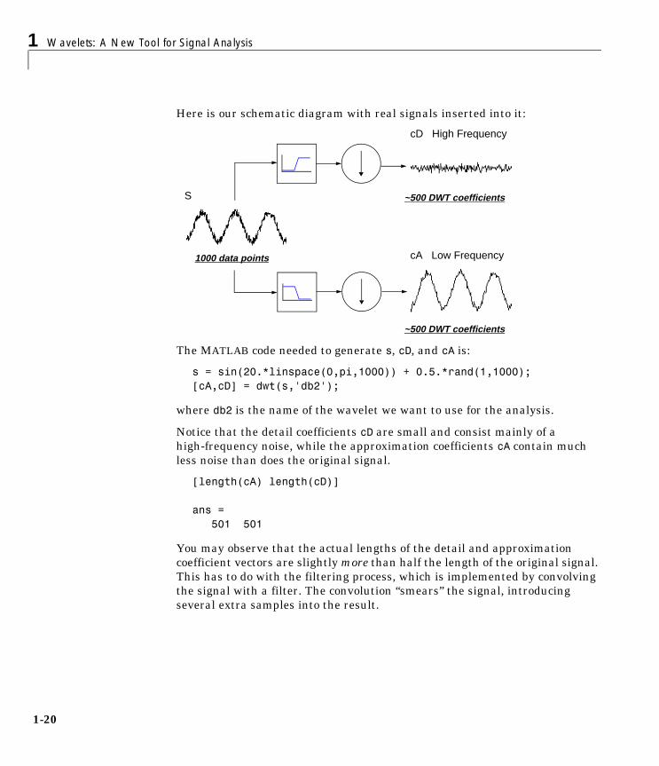
Here is our schematic diagram with real signals inserted into it:

The MATLAB code needed to generate s, cD, and cA is:

s = sin(20.*linspace(0,pi,1000)) + 0.5.*rand(1,1000);[cA,cD] = dwt(s,'db2');

where db2 is the name of the wavelet we want to use for the analysis.

Notice that the detail coefficients cD are small and consist mainly of a high-frequency noise, while the approximation coefficients cA contain much less noise than does the original signal.

[length(cA) length(cD)]

ans = 501 501

You may observe that the actual lengths of the detail and approximation coefficient vectors are slightly more than half the length of the original signal. This has to do with the filtering process, which is implemented by convolving the signal with a filter. The convolution “smears” the signal, introducing several extra samples into the result.

1000 data points

~500 DWT coefficients

~500 DWT coefficients

S

cD High Frequency

cA Low Frequency

The Discrete Wavelet Transform

1-21

Multiple-Level DecompositionThe decomposition process can be iterated, with successive approximations being decomposed in turn, so that one signal is broken down into many lower resolution components. This is called the wavelet decomposition tree.

Looking at a signal’s wavelet decomposition tree can yield valuable information.

Number of LevelsSince the analysis process is iterative, in theory it can be continued indefinitely. In reality, the decomposition can proceed only until the individual details consist of a single sample or pixel. In practice, you’ll select a suitable number of levels based on the nature of the signal, or on a suitable criterion such as entropy (see “Choosing the Optimal Decomposition” on page 6-137).

S

cA1 cD1

cA2 cD2

cA3 cD3

S

cA1 cD1

cA2 cD2

cA3 cD3


1-22

Wavelet ReconstructionWe’ve learned how the discrete wavelet transform can be used to analyze, or decompose, signals and images. This process is called decomposition or analysis. The other half of the story is how those components can be assembled back into the original signal without loss of information. This process is called reconstruction, or synthesis. The mathematical manipulation that effects synthesis is called the inverse discrete wavelet transform (IDWT).

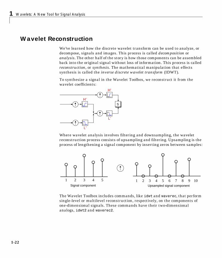
To synthesize a signal in the Wavelet Toolbox, we reconstruct it from the wavelet coefficients:

Where wavelet analysis involves filtering and downsampling, the wavelet reconstruction process consists of upsampling and filtering. Upsampling is the process of lengthening a signal component by inserting zeros between samples:

The Wavelet Toolbox includes commands, like idwt and waverec, that perform single-level or multilevel reconstruction, respectively, on the components of one-dimensional signals. These commands have their two-dimensional analogs, idwt2 and waverec2.

S

H’

L’

H’

L’

Signal component Upsampled signal component

1 2 3 4 5 1 2 3 4 5 6 7 8 9 10

Wavelet Reconstruction

1-23

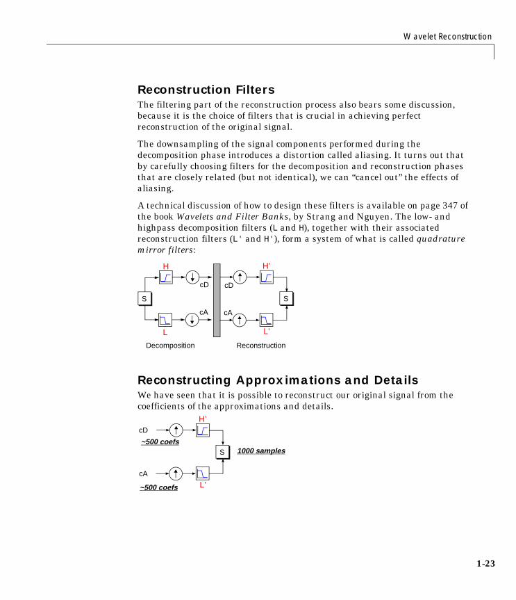
Reconstruction FiltersThe filtering part of the reconstruction process also bears some discussion, because it is the choice of filters that is crucial in achieving perfect reconstruction of the original signal.

The downsampling of the signal components performed during the decomposition phase introduces a distortion called aliasing. It turns out that by carefully choosing filters for the decomposition and reconstruction phases that are closely related (but not identical), we can “cancel out” the effects of aliasing.

A technical discussion of how to design these filters is available on page 347 of the book Wavelets and Filter Banks, by Strang and Nguyen. The low- and highpass decomposition filters (L and H), together with their associated reconstruction filters (L' and H'), form a system of what is called quadrature mirror filters:

Reconstructing Approximations and DetailsWe have seen that it is possible to reconstruct our original signal from the coefficients of the approximations and details.

S S

Decomposition Reconstruction

H

L

H’

L’

cD

cA

cD

cA

S

H’

L’

cD

cA

1000 samples~500 coefs

~500 coefs


1-24

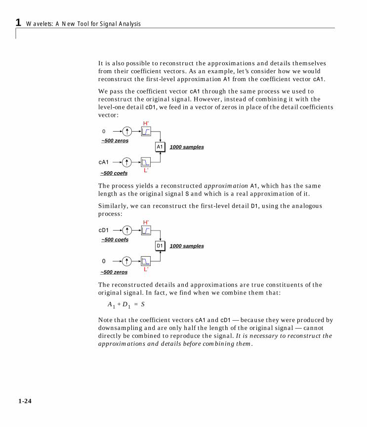
It is also possible to reconstruct the approximations and details themselves from their coefficient vectors. As an example, let’s consider how we would reconstruct the first-level approximation A1 from the coefficient vector cA1.

We pass the coefficient vector cA1 through the same process we used to reconstruct the original signal. However, instead of combining it with the level-one detail cD1, we feed in a vector of zeros in place of the detail coefficients vector:

The process yields a reconstructed approximation A1, which has the same length as the original signal S and which is a real approximation of it.

Similarly, we can reconstruct the first-level detail D1, using the analogous process:

The reconstructed details and approximations are true constituents of the original signal. In fact, we find when we combine them that:

Note that the coefficient vectors cA1 and cD1 — because they were produced by downsampling and are only half the length of the original signal — cannot directly be combined to reproduce the signal. It is necessary to reconstruct the approximations and details before combining them.

A1

H’

L’

0

cA1

1000 samples~500 zeros

~500 coefs

D1

H’

L’

cD1

0

1000 samples~500 coefs

~500 zeros

A1 D1+ S=


1-25

Extending this technique to the components of a multilevel analysis, we find that similar relationships hold for all the reconstructed signal constituents. That is, there are several ways to reassemble the original signal:

Relationship of Filters to Wavelet ShapesIn the section “Reconstruction Filters” on page 1-23, we spoke of the importance of choosing the right filters. In fact, the choice of filters not only determines whether perfect reconstruction is possible, it also determines the shape of the wavelet we use to perform the analysis.

To construct a wavelet of some practical utility, you seldom start by drawing a waveform. Instead, it usually makes more sense to design the appropriate quadrature mirror filters, and then use them to create the waveform. Let’s see how this is done by focusing on an example.

Consider the lowpass reconstruction filter (L') for the db2 wavelet.

The filter coefficients can be obtained from the dbaux command:

Lprime = dbaux(2)

Lprime = 0.3415 0.5915 0.1585 –0.0915

S

A1 D1

A2 D2

A3 D3

= A2 D2 D1+ +

S A1 D1+=

= A3 D3 D2 D1+ + +

ReconstructedSignal

Components

0 1 2 3

−1

0

1

db2 wavelet


1-26

If we reverse the order of this vector (see wrev), and then multiply every even sample by –1, we obtain the highpass filter H':

Hprime = –0.0915 –0.1585 0.5915 –0.3415

Next, upsample Hprime by two (see dyadup), inserting zeros in alternate positions:

HU = –0.0915 0 –0.1585 0 0.5915 0 –0.3415 0

Finally, convolve the upsampled vector with the original lowpass filter:

H2 = conv(HU,Lprime);plot(H2)

If we iterate this process several more times, repeatedly upsampling and convolving the resultant vector with the four-element filter vector Lprime, a pattern begins to emerge:

1 2 3 4 5 6 7 8 9 10

−0.2

−0.1

0

0.1

0.2

0.3

5 10 15 20

−0.1−0.05

00.050.1

0.15

Second Iteration

10 20 30 40

−0.05

0

0.05

0.1Third Iteration

20 40 60 80−0.04

−0.02

0

0.02

0.04

Fourth Iteration

50 100 150−0.02

−0.01

0

0.01

0.02

Fifth Iteration


1-27

The curve begins to look progressively more like the db2 wavelet. This means that the wavelet’s shape is determined entirely by the coefficients of the reconstruction filters.

This relationship has profound implications. It means that you cannot choose just any shape, call it a wavelet, and perform an analysis. At least, you can’t choose an arbitrary wavelet waveform if you want to be able to reconstruct the original signal accurately. You are compelled to choose a shape determined by quadrature mirror decomposition filters.

The Scaling FunctionWe’ve seen the interrelation of wavelets and quadrature mirror filters. The wavelet function is determined by the highpass filter, which also produces the details of the wavelet decomposition.

There is an additional function associated with some, but not all wavelets. This is the so-called scaling function, . The scaling function is very similar to the wavelet function. It is determined by the lowpass quadrature mirror filters, and thus is associated with the approximations of the wavelet decomposition.

In the same way that iteratively upsampling and convolving the highpass filter produces a shape approximating the wavelet function, iteratively upsampling and convolving the lowpass filter produces a shape approximating the scaling function.

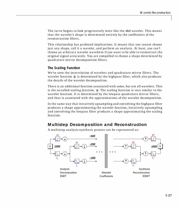
Multistep Decomposition and ReconstructionA multistep analysis-synthesis process can be represented as:

ψ

φ

S 1000~250

~250

S1000

~500

AnalysisDecompositionDWT

SynthesisReconstruction

IDWTWavelet

Coefficients

. . . . . .

H

L

H

L

H’

L’

H’

L’


1-28

This process involves two aspects: breaking up a signal to obtain the wavelet coefficients, and reassembling the signal from the coefficients.

We’ve already discussed decomposition and reconstruction at some length. Of course, there is no point breaking up a signal merely to have the satisfaction of immediately reconstructing it. We may modify the wavelet coefficients before performing the reconstruction step. We perform wavelet analysis because the coefficients thus obtained have many known uses, de-noising and compression being foremost among them.

But wavelet analysis is still a new and emerging field. No doubt, many uncharted uses of the wavelet coefficients lie in wait. The Wavelet Toolbox can be a means of exploring possible uses and hitherto unknown applications of wavelet analysis. Explore the toolbox functions and see what you discover.

Wavelet Packet Analysis

1-29

Wavelet Packet AnalysisThe wavelet packet method is a generalization of wavelet decomposition that offers a richer range of possibilities for signal analysis.

In wavelet analysis, a signal is split into an approximation and a detail. The approximation is then itself split into a second-level approximation and detail, and the process is repeated. For an n-level decomposition, there are n+1 possible ways to decompose or encode the signal.

In wavelet packet analysis, the details as well as the approximations can be split.

This yields more than different ways to encode the signal. This is the wavelet packet decomposition tree.

The wavelet decomposition tree is a part of this complete binary tree.

For instance, wavelet packet analysis allows the signal S to be represented as A1 + AAD3 + DAD3 + DD2. This is an example of a representation that is not possible with ordinary wavelet analysis.

S

A1 D1

A2 D2

A3 D3

= A2 D2 D1+ +

S A1 D1+=

= A3 D3 D2 D1+ + +

22n 1–

S

A1 D1

AA2 DA2

AAA3 DAA3

AD2 DD2

ADA3 DDA3 AAD3 DAD3 ADD3 DDD3


1-30

Choosing one out of all these possible encodings presents an interesting problem. In this toolbox, we use an entropy-based criterion to select the most suitable decomposition of a given signal. This means we look at each node of the decomposition tree and quantify the information to be gained by performing each split.

Simple and efficient algorithms exist for both wavelet packet decomposition and optimal decomposition selection. This toolbox uses an adaptive filtering algorithm, based on work by Coifman and Wickerhauser (see [CoiW92] in “References” on page 6-145), with direct applications in optimal signal coding and data compression.

Such algorithms allow the Wavelet Packet 1-D and Wavelet Packet 2-D tools to include “Best Level” and “Best Tree” features that optimize the decomposition both globally and with respect to each node.

History of Wavelets

1-31

History of WaveletsFrom an historical point of view, wavelet analysis is a new method, though its mathematical underpinnings date back to the work of Joseph Fourier in the nineteenth century. Fourier laid the foundations with his theories of frequency analysis, which proved to be enormously important and influential.

The attention of researchers gradually turned from frequency-based analysis to scale-based analysis when it started to become clear that an approach measuring average fluctuations at different scales might prove less sensitive to noise.

The first recorded mention of what we now call a “wavelet” seems to be in 1909, in a thesis by Alfred Haar.

The concept of wavelets in its present theoretical form was first proposed by Jean Morlet and the team at the Marseille Theoretical Physics Center working under Alex Grossmann in France.

The methods of wavelet analysis have been developed mainly by Y. Meyer and his colleagues, who have ensured the methods’ dissemination. The main algorithm dates back to the work of Stephane Mallat in 1988. Since then, research on wavelets has become international. Such research is particularly active in the United States, where it is spearheaded by the work of scientists such as Ingrid Daubechies, Ronald Coifman, and Victor Wickerhauser.

Barbara Burke Hubbard describes the birth, the history and the seminal concepts in a very clear text. See “The World According to Wavelets” A.K. Peters Wellesley 1996.

The wavelet domain is growing up very quickly. A lot of mathematical papers and practical trials are published every month.

Wavelet Applications - umu.se · Wavelet Applications 1-3 Wavelet Applications Wavelets have scale...

Documents

Transcript of Wavelet Applications - umu.se · Wavelet Applications 1-3 Wavelet Applications Wavelets have scale...