Water Resources Engineering Program - غزةlibrary.iugaza.edu.ps/thesis/87432.pdfWater Resources...
130
Water Resources Engineering Program The Islamic University – Gaza High Studies Deanery Faculty of Engineering Study The Impact of Land Use and Over Pumping on Nitrate Concentration in Groundwater by Using Modeling Approach Case Study: Khanyounis Governorate- Gaza Strip August, 2009 Supervised by: Dr. Abdelmajid Nassar, Dr. Khaled Qahman Master dissertation in partial of fulfillment of the requirement for the degree of Master of science in water resources engineering. By: Rami J. H. Alghamri
Transcript of Water Resources Engineering Program - غزةlibrary.iugaza.edu.ps/thesis/87432.pdfWater Resources...
Water Resources Engineering Program
The Islamic University – Gaza
High Studies Deanery
Faculty of Engineering
Study The Impact of Land Use and Over Pumping on Nitrate
Concentration in Groundwater by Using Modeling Approach
Case Study: Khanyounis Governorate- Gaza Strip
August, 2009 Supervised by:
Dr. Abdelmajid Nassar, Dr. Khaled Qahman
Master dissertation in partial of fulfillment of the requirement for the degree of
Master of science in water resources engineering. By:
Rami J. H. Alghamri

I
This Thesis is dedicated to
My Mother, Father, Wife and child

II
ACKNOWLEDGMENTS
First of all, thanks God for his care and grace.
I would like to extend my deepest and humble gratitude to my promoters Dr. Abdelmajid
Nassar and Dr. Khaled Qahman for there invaluable supervision, helpful suggestions
and priceless support during the period of my study. Thank you very much.
Also, I send my deepest thanks to the whole staff of civil engineering department in the
Islamic University of Gaza, especially those who taught me.
I wish to express my deepest thanks to Eng. Rana Jaber for her great help, invaluable remarks
and suggestions.
Special thanks and appreciation go to my dear friend Khalil Al-Astal for his encouragement
and support. Additionally, thanks go to my colleagues in the water resources engineering
program.
My ultimate respect and appreciation to all my family members, especially my father and
mother for their moral support and their faithful prayers.
I would like to thank my beautiful wife Asmaa' for her love, care and support throughout my
study. Asmaa, you are really the pillar of my life.
Last not but least to my lovely and wonderful son Jasser. You always bring inspiration,
meaning and purpose to my life, I love you.
Rami Alghamri
August, 2009
III
TABLE OF CONTENTS
I DEDICATION
II ACKNOWLEDGMENTS
III TABLE OF CONTENTS
VII LIST OF FIGURES
IX LIST OF TABLES
XI LIST OF SYMBOLS
XII LIST OF ABBREVIATIONS
XIII ABSTRACT
XIV ARABIC ABSTRACT 1-6 CHAPTER 1: INTRODUCTION
2 Background 1.1
3 Problem Identification 1.2
4 Research Objectives 1.3
4 Methodology 1.4
5 Thesis Structure 1.5
7-30 CHAPTER 2: LITERATURE REVIEW 8 Nitrate in Groundwater 2.1
8 WHO Standards 2.1.1
8 The Environmental Health Concerns of Nitrate in Drinking Water 2.1.2
9 The Nitrogen Cycle 2.1.3
9 Nitrogen Fixation 2.1.3.1
10 Mineralization-Immobilization 2.1.3.2
10 Nitrification 2.1.3.3
11 Ammonia volatilization 2.1.3.4
11 Adsorption 2.1.3.5
12 Denitrification 2.1.3.6
12 Sources of Nitrogen in Soil 2.1.4
13 Nitrate Leaching 2.1.5
13 Factors Affecting Leaching 2.1.5.1
14 Nitrate Transport Mechanisms 2.1.5.2
14 On-Ground Nitrogen Loading 2.1.6
IV
15 Effluent from sewer systems and septage 2.1.6.1
15 Leachate From landfills 2.1.6.2
16 Fertilizers 2.1.6.3
16 Manure N Inputs 2.1.6.4
16 Irrigation Water Inputs 2.1.6.5
17 Nitrogen Fixation Inputs 2.1.6.6
17 Precipitation Inputs 2.1.6.7
17 Losses of Nitrogen 2.1.7
17 Losses Through Ammonia Volatilization 2.1.7.1
18 Losses through Denitrification 2.1.7.2
18 Plant Uptake 2.1.7.3
19 Erosion and runoff 2.1.7.4
19 Groundwater Modelling 2.2
19 General Groundwater Flow Equations 2.2.1
20 Numerical Methods of Solving Flow Equations 2.2.2
20 Solute Transport 2.2.3
21 Numerical Methods of Solute Transport Equations 2.2.4
22 Related Studies 2.3
31-47CHAPTER 3: STUDY AREA 32 Introduction 3.1
34 Physical Settings 3.2
34 Climate 3.2.1
35 Temperature, Humidity and Solar Radiation 3.2.1.1
35 Rainfall 3.2.1.2
36 Reference Crop Evapotranspiration (ETo) 3.2.1.3
37 Topography and Soil 3.2.2
39 Land Use 3.2.3
40 Hydrogeology 3.3
40 Description of the Coastal Aquifer 3.3.1
41 Aquifer Hydraulic Properties 3.3.2
41 Groundwater Flow and Water Levels 3.3.3
42 Water Quality 3.4
42 Groundwater Salinity (Chloride) 3.4.1
44 Nitrate Pollution 3.4.2
V
45 Description of Existing Sewerage Situation 3.5
48-77CHAPTER 4: GROUNDWATER MODELING 49 Introduction 4.1
49 Modeling Code and Principles 4.2
50 MODFLOW 4.2.1
51 MODPATH 4.2.2
51 MT3DMS 4.2.3
51 Data Management 4.3
52 The Aquifer Hydrogeology 4.3.1
53 Water Quality Data 4.3.2
53 Water Level Data 4.3.3
53 Conceptual Model 4.4
54 Model Construction 4.5
56 Internal Hydrologic Stresses 4.6
56 Recharge from Precipitation 4.6.1
58 Pumping Wells 4.6.2
59 Return Flows 4.6.3
60 Water Balance 4.7
60 Initial Conditions 4.8
60 Model Calibration 4.9
61 Steady State Calibration 4.9.1
62 Calibrated Mass Balance 4.9.1.1
63 Calibrated Parameters 4.9.1.2
67 Transient Calibration 4.9.2
72 Comparison of Results Between This Study and Some Related Studies 4.10
73 Transport Model 4.11
73 Assumptions for The Transport Model 4.11.1
73 Calibration of Transport Model 4.11.2
78-94CHAPTER 5: MANAGEMENT SCENARIOS 79 Introduction 5.1
79 Management Scenarios 5.2
80 Assumptions for All Scenarios 5.2.1
81 Results and Discussion 5.3
93 Comparison between all scenarios 5.4
VI
95-97CHAPTER 6: CONCLUSION AND RECOMMENDATIONS 96 Conclusion 6.1
97 Recommendations 6.2
97 Suggested complementary studies 6.3
98-104 REFERENCES
106-115 APPENDIX
VII
LIST OF FIGURES
Figure Description Page
1.1 Schematic diagram of study methodology 5
2.1 The Nitrogen Cycle 9
3.1 Geographic location of the Gaza Strip 32
3.2 Gaza Strip Governorates 33
3.3 Khanyounis map 34
3.4 Mean monthly maximum, minimum and average temperature (C°)for the Gaza
Strip
35
3.5 Locations of rain stations in the Gaza Strip 37
3.6 Topography of Khanyounis 38
3.7 Soil map of Gaza Strip 38
3.8 Regional plan for Gaza Governorates 39
3.9 Generalized Cross-Section of the Coastal Plain 40
3.10 Water level elevation map for hydrological year 2007/2008 42
3.11 Chloride concentration map for the year 2007 44
3.12 Nitrate concentration map for the year 2007 45
3.13 Scheme for Khanyounis governorate waste water network 46
3.14 Waste water discharged to the existing storm water ponds at Al Amal Area-
Khanyounis
47
4.1 Chart of the modeling process 50
4.2 Gaza Strip with geological cross-sections drawn by Israelis in 1979 52
4.3 Geological cross-section sample, along strip 83 53
4.4 Groundwater levels of the coastal aquifer in Gaza Strip from the mean sea level
for the year 2004
54
4.5 The model domain with the grid origin, orientation and boundaries 55
4.6 A vertical representation of the discretization of the model. Clay layers do not
extend the full length of layer to signify their limited pinch out inland
56
4.7 Vertical cross section through model 56
4.8 (a) Distribution of rainfall stations and zones
(b) Recharge coefficients
57
4.9 Wells distribution in southern Gaza Strip within model domain 59
4.10 Simulated groundwater table for year 1935-calculated by VMODFLOW 61
4.11 Calibrated versus measured groundwater levels at the end of year 1935 62
VIII
4.12 Distribution of head observation wells within the model area 64
4.13 Simulated water table for year 2004-calculated by VMODFLOW 65
4.14 Calculated vs. observed heads and summary of steady state calibration statistics
(year 2004)
66
4.15 Calibrated versus measured groundwater levels at the end of year 2005 68
4.16 Calibrated versus measured groundwater levels at the end of year 2006 68
4.17 Calibrated versus measured groundwater levels at the end of year 2007 69
4.18 Calibrated versus measured groundwater levels at the end of year 2008 69
4.19 Observed and calculated heads versus time for well Y4 70
4.20 Observed and calculated heads versus time for well L.94 70
4.21 Observed and calculated heads versus time for well L.18 71
4.22 Observed and calculated heads versus time for well N.16 71
4.23 Calculated versus observed NO-3 concentration at the end of 2005 74
4.24 Calculated versus observed NO-3 concentration at the end of 2006 75
4.25 Calculated versus observed NO-3 concentration at the end of 2007 75
4.26 Calculated versus observed NO-3 concentration at the end of 2008 76
4.27 Calibrated NO-3 concentrations within southern Gaza Strip for the end of year
2008(mg/l)
77
5.1 Selected observation wells distribution in southern Gaza Strip within model
domain for management scenarios
82
5.2 Nitrate concentrations versus scenarios 1 and 3 (2008-2038) for well L.159 86
5.3 Nitrate concentrations versus scenarios 1 and 4 (2008-2038) for well N.16 87
5.4 Nitrate concentrations versus scenarios 1 and 4 (2008-2038) for well L.159 88
5.5 Nitrate concentrations versus scenarios 1 and 5 (2008-2038) for well L.159 89
5.6 Nitrate concentrations versus scenarios 1 and 5 (2008-2038) for well N.16 90
5.7 Infiltration sites at Khanyounis governorate 91
5.8 Schematic drawing of the component of the wastewater reuse system proposed to
implement in Khanyounis
91
5.9 Average simulated nitrate concentrations versus management scenarios (2008-
2038)
94
A-1 land use map of southern Gaza Strip 107
IX
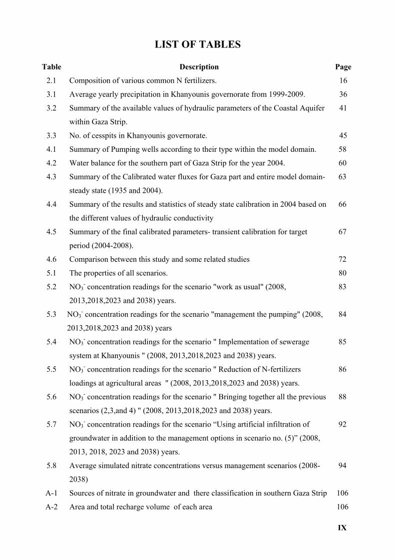
LIST OF TABLES
Table Description Page
2.1 Composition of various common N fertilizers. 16
3.1 Average yearly precipitation in Khanyounis governorate from 1999-2009. 36
3.2 Summary of the available values of hydraulic parameters of the Coastal Aquifer
within Gaza Strip.
41
3.3 No. of cesspits in Khanyounis governorate. 45
4.1 Summary of Pumping wells according to their type within the model domain. 58
4.2 Water balance for the southern part of Gaza Strip for the year 2004. 60
4.3 Summary of the Calibrated water fluxes for Gaza part and entire model domain-
steady state (1935 and 2004).
63
4.4 Summary of the results and statistics of steady state calibration in 2004 based on
the different values of hydraulic conductivity
66
4.5 Summary of the final calibrated parameters- transient calibration for target
period (2004-2008).
67
4.6 Comparison between this study and some related studies 72
5.1 The properties of all scenarios. 80
5.2 NO3- concentration readings for the scenario "work as usual" (2008,
2013,2018,2023 and 2038) years.
83
5.3 NO3- concentration readings for the scenario "management the pumping" (2008,
2013,2018,2023 and 2038) years
84
5.4 NO3- concentration readings for the scenario " Implementation of sewerage
system at Khanyounis " (2008, 2013,2018,2023 and 2038) years.
85
5.5 NO3- concentration readings for the scenario " Reduction of N-fertilizers
loadings at agricultural areas " (2008, 2013,2018,2023 and 2038) years.
86
5.6 NO3- concentration readings for the scenario " Bringing together all the previous
scenarios (2,3,and 4) " (2008, 2013,2018,2023 and 2038) years.
88
5.7 NO3- concentration readings for the scenario “Using artificial infiltration of
groundwater in addition to the management options in scenario no. (5)” (2008,
2013, 2018, 2023 and 2038) years.
92
5.8 Average simulated nitrate concentrations versus management scenarios (2008-
2038)
94
A-1 Sources of nitrate in groundwater and there classification in southern Gaza Strip 106
A-2 Area and total recharge volume of each area 106
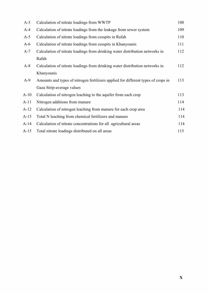
X
A-3 Calculation of nitrate loadings from WWTP 108
A-4 Calculation of nitrate loadings from the leakage from sewer system 109
A-5 Calculation of nitrate loadings from cesspits in Rafah 110
A-6 Calculation of nitrate loadings from cesspits in Khanyounis 111
A-7 Calculation of nitrate loadings from drinking water distribution networks in
Rafah
112
A-8 Calculation of nitrate loadings from drinking water distribution networks in
Khanyounis
112
A-9 Amounts and types of nitrogen fertilizers applied for different types of crops in
Gaza Strip-average values
113
A-10 Calculation of nitrogen leaching to the aquifer from each crop 113
A-11 Nitrogen additions from manure 114
A-12 Calculation of nitrogen leaching from manure for each crop area 114
A-13 Total N leaching from chemical fertilizers and manure 114
A-14 Calculation of nitrate concentrations for all agricultural areas 114
A-15 Total nitrate loadings distributed on all areas 115
XI
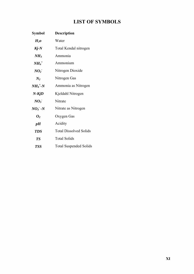
LIST OF SYMBOLS
Symbol Description
H2o Water
Kj-N Total Kendal nitrogen
NH3 Ammonia
NH4+ Ammonium
NO2- Nitrogen Dioxide
N2 Nitrogen Gas
NH4+-N Ammonia as Nitrogen
N-KjD Kjeldahl Nitrogen
NO3- Nitrate
NO3- -N Nitrate as Nitrogen
O2 Oxygen Gas
pH Acidity
TDS Total Dissolved Solids
TS Total Solids
TSS Total Suspended Solids
XII
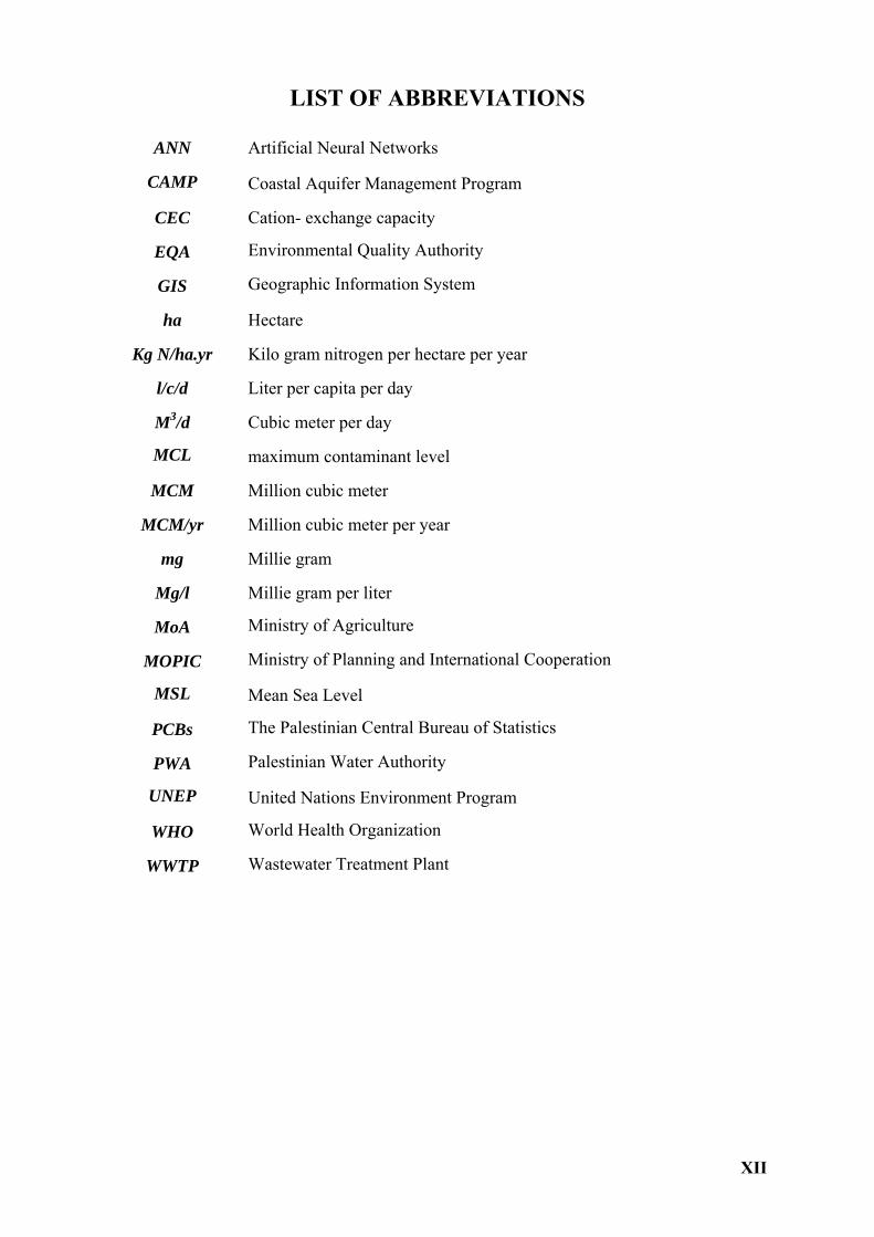
LIST OF ABBREVIATIONS
ANN Artificial Neural Networks
CAMP Coastal Aquifer Management Program
CEC Cation- exchange capacity
EQA Environmental Quality Authority
GIS Geographic Information System
ha Hectare
Kg N/ha.yr Kilo gram nitrogen per hectare per year
l/c/d Liter per capita per day
M3/d Cubic meter per day
MCL maximum contaminant level
MCM Million cubic meter
MCM/yr Million cubic meter per year
mg Millie gram
Mg/l Millie gram per liter
MoA Ministry of Agriculture
MOPIC Ministry of Planning and International Cooperation
MSL Mean Sea Level
PCBs The Palestinian Central Bureau of Statistics
PWA Palestinian Water Authority
UNEP United Nations Environment Program
WHO World Health Organization
WWTP Wastewater Treatment Plant
XIII
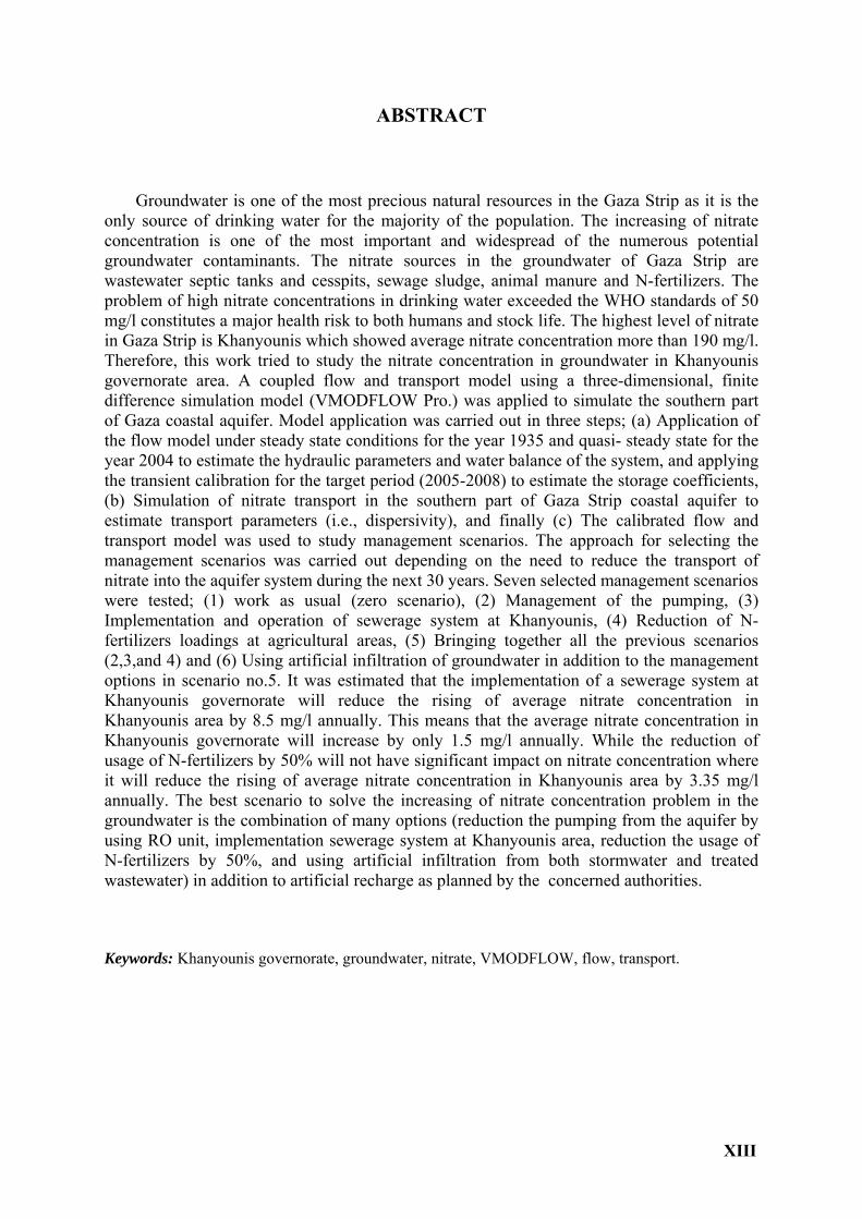
ABSTRACT
Groundwater is one of the most precious natural resources in the Gaza Strip as it is the only source of drinking water for the majority of the population. The increasing of nitrate concentration is one of the most important and widespread of the numerous potential groundwater contaminants. The nitrate sources in the groundwater of Gaza Strip are wastewater septic tanks and cesspits, sewage sludge, animal manure and N-fertilizers. The problem of high nitrate concentrations in drinking water exceeded the WHO standards of 50 mg/l constitutes a major health risk to both humans and stock life. The highest level of nitrate in Gaza Strip is Khanyounis which showed average nitrate concentration more than 190 mg/l. Therefore, this work tried to study the nitrate concentration in groundwater in Khanyounis governorate area. A coupled flow and transport model using a three-dimensional, finite difference simulation model (VMODFLOW Pro.) was applied to simulate the southern part of Gaza coastal aquifer. Model application was carried out in three steps; (a) Application of the flow model under steady state conditions for the year 1935 and quasi- steady state for the year 2004 to estimate the hydraulic parameters and water balance of the system, and applying the transient calibration for the target period (2005-2008) to estimate the storage coefficients, (b) Simulation of nitrate transport in the southern part of Gaza Strip coastal aquifer to estimate transport parameters (i.e., dispersivity), and finally (c) The calibrated flow and transport model was used to study management scenarios. The approach for selecting the management scenarios was carried out depending on the need to reduce the transport of nitrate into the aquifer system during the next 30 years. Seven selected management scenarios were tested; (1) work as usual (zero scenario), (2) Management of the pumping, (3) Implementation and operation of sewerage system at Khanyounis, (4) Reduction of N-fertilizers loadings at agricultural areas, (5) Bringing together all the previous scenarios (2,3,and 4) and (6) Using artificial infiltration of groundwater in addition to the management options in scenario no.5. It was estimated that the implementation of a sewerage system at Khanyounis governorate will reduce the rising of average nitrate concentration in Khanyounis area by 8.5 mg/l annually. This means that the average nitrate concentration in Khanyounis governorate will increase by only 1.5 mg/l annually. While the reduction of usage of N-fertilizers by 50% will not have significant impact on nitrate concentration where it will reduce the rising of average nitrate concentration in Khanyounis area by 3.35 mg/l annually. The best scenario to solve the increasing of nitrate concentration problem in the groundwater is the combination of many options (reduction the pumping from the aquifer by using RO unit, implementation sewerage system at Khanyounis area, reduction the usage of N-fertilizers by 50%, and using artificial infiltration from both stormwater and treated wastewater) in addition to artificial recharge as planned by the concerned authorities.
Keywords: Khanyounis governorate, groundwater, nitrate, VMODFLOW, flow, transport.
XIV
الملخص
تأثير استخدام األراضي وزيادة السحب من الخزان الجوفي على تركيز النترات في المياه الجوفيةنمذجة
) جنوب قطاع غزة -سمحافظة خانيون: حالة الدراسة(
. لمصادر الطبيعية للمياه في قطاع غزة، كما أنها المصدر الوحيد للشرب لغالبية سكان القطاع تعتبر المياه الجوفية أحد أهم ا
يعزى ارتفاع تركيز النتـرات فـي الخـزان . النترات واحدة من أهم الملوثات التي يعاني منها الخزان الجوفي في القطاع
تسرب المياه العادمة من الحفر االمتـصاصية، أو :الجوفي إلى استخدام األراضي في ذات المنطقة ومن أهم مصادر التلوث
.شبكات الصرف الصحي، وكذلك األنشطة الزراعية بما تحويه من أسمدة ومبيدات تحتوي على النترات بشكل كبير
وفق منظمة الصحة العالمية تؤثر سلباً على صحة اإلنـسان ترل / لليغرامم 50التركيزات المرتفعة للنترات والتي تزيد عن
/ لليغرامم 190تعتبر محافظة خانيونس األكثر تأثراً بمشكلة النترات في الخزان الجوفي حيث يصل لما يزيد عن . لحيوانوا
تر، لذلك فإن هذه الدراسة ركزت على مشكلة النترات في محافظة خانيونس وسبل إيجاد الحلول المناسـبة لعالجهـا مـع ل
.دراسة أهم المؤثرات عليها
لمحاكاة التدفق واالنتقال في المياه الجوفيـة للمنطقـة (.VMODFLOW Pro) ج المحاكاة ثالثي األبعادتم استخدام نموذ
تطبيـق النمـوذج تحـت ) أ: (مع تطبيق النموذج على ثالث مراحل ) بما يشمل محافظة خانيونس (الجنوبية من قطاع غزة
ص الهيدرولوجية للخزان الجوفي، وكذلك التوازن بهدف تقدير الخوا 2004، وكذلك عام 1935ظروف التدفق المطرد لعام
، )2008-2005(المائي للنظام، ثم تطبيق النموذج لتقدير معامالت التخزين للخزان الجوفي تحت ظروف المعايرة في الفترة
ام النموذج بعد استخد) ج(محاكاة انتقال النترات داخل المياه الجوفية لتحديد معامالت االنتقال الخاصة بالخزان الجوفي، ) ب(
معايرته لدراسة السيناريوهات المختلفة نحو إدارة الخزان الجوفي بما يتعلق بمشكلة النترات، وذلك خـالل الثالثـين عـام
.القادمة
إدارة الـسحب مـن الخـزان ) 2(االستمرار في الوضع القائم، ) 1: (سيناريوهات تم دراستها خالل هذا العمل، وهي ستة
تخفيـف ) 4(تنفيذ شبكة الصرف الصحي في خانيونس وتشغيلها بكل مكوناتهـا، ) 3(ائل لهذا المصدر، الجوفي بإيجاد البد
الجمع بين السيناريوهات السابقة ) 5( المحتوية على النترات أو مشتقات النيتروجين في المناطق الزراعية، األسمدةاستخدام
.لعادمة بعد معالجتها باإلضافة للسيناريو السابقحقن الخزان الجوفي بمياه األمطار والمياه ا) 6(، "2،3،4"
وفق نتائج الدراسة فإن تنفيذ وتشغيل شبكة الصرف الصحي وفق المخطط له من ِقبل المؤسسات المختصة سيقلل من تركيز
تر مقارنةً ل/ لليغرامم 8.5تر، أي سيقلل الزيادة في تركيز النترات السنوي بمقدار ل / لليغرامم 1.5النترات سنوياً بمقدار
.مع االستمرار بالوضع القائم
المحتوية على النترات أو مشتقات النيتروجين في المناطق الزراعية سيكون له تأثير بسيط على تخفيف استخدام األسمدة أما
.القائمتر مقارنةً مع االستمرار بالوضع ل / لليغرامم 3.35تركيز النترات حيث سيقلل الزيادة السنوية بما ال يتجاوز
تشغيل شبكة الصرف الصحي، وإدارة الـسحب مـن الخـزان (الجمع بين جميع السيناريوهات أما السيناريو األفضل فهو
مع حقن الخزان الجوفي بمياه األمطـار )الجوفي، وتخفيف استخدام األسمدة المحتوية على النترات أو مشتقات النيتروجين
المتوقع أن يصل بالنترات إلى تركيز يقارب القيمة التي تنص عليها منظمة الـصحة ، وهذا من والمياه العادمة بعد معالجتها
. العالمية
Chapter1: Introduction
1
CHAPTER 1
INTRODUCTION
Chapter1: Introduction
2
CHAPTER 1: INTRODUCTION
1.1 Background Groundwater is one of the most precious natural resources in the Gaza Strip as it is the
only source of drinking water for the majority of the population (Shomar et. al., 2005). It is
utilized extensively to satisfy agricultural, domestic, and industrial water demands.
Groundwater crisis in Gaza includes two major folds: shortage and contamination. The
extraction of groundwater currently exceeds the aquifer recharge rate. As a result, the
groundwater level is falling continuously and accompanied with it the contamination with
many pollutants mainly nitrate and seawater intrusion (UNEP, 2003; Weinthal and Vengosh,
2005; Qahman and Larabi, 2006).
The manmade sources of pollution endanger the water resources supplies in the major
municipalities of the Gaza Strip. Many water quality parameters in the Gaza aquifer presently
exceed the maximum contaminant level of the WHO drinking water standards, especially for
nitrate and chloride. Chloride or salinity of the groundwater increases by time due to seawater
intrusion and mobilization of incident deep brackish water, caused by over-abstraction of the
groundwater (Rocca et. al., 2005).
Nitrate is one of the most important and widespread of the numerous potential
groundwater contaminants (Rocca et. al., 2005). Contamination of the groundwater can occur
if input of NO3- into soil exceeds the consumption of plants and denitrification (Mcclain et
al., 1994). Shomar (2006) proposed that the excess NO3- in the groundwater of the Gaza Strip
occurred as a result of NO3- leaching from irrigation, wastewater septic tanks, sewage sludge,
animal manure and synthetic fertilizers.
The problem of high nitrate concentrations in drinking water constitutes a major health
risk to both humans and stock life. Nitrite reacts directly with hemoglobin in human blood
and other warm-blooded animals to produce methaemoglobin. Methaemoglobin destroys the
ability of red blood cells to transport oxygen. This condition is especially serious for babies.
It causes a condition known as methaemoglobinemia or “blue baby” disease. The WHO
assigned the nitrate of 50 mg/l as a health significant value in drinking water (Khayat et. al.,
2006).
Chapter1: Introduction
3
1.2 Problem Identification Almost 90% of the groundwater wells of the Gaza Strip sampled between 2001 and 2007
showed NO3- concentrations two to eight times higher than the WHO standards. The highest
levels of NO3- were in Khanyounis (south) and Jabalia (north). These regions showed average
NO3- concentrations of 191 and 151 mg/l, respectively (Shomar et. al., 2008). In the worst
affected areas (urban centers), NO3- concentrations are increasing at rates of up to 10 mg/l per
year (Mogheir, 2005). This means that the level of nitrate contamination is rising so rapidly
and continuously that most of Gaza's domestic wells are no longer adequate for human
consumption due to this very poor quality unless serious solutions and management
protections are used to face the present and future challenges (Jaber, 2008).
The main sources of the high nitrate pollution of groundwater in Gaza Strip are
infiltration of untreated wastewater in cesspits and excess agricultural fertilizers, where about
40% of the population uses leaky infiltration boreholes, and the rest uses inadequate sewage
system (Metcalf and Eddy, 2000). According to personal contacts, about 60% of Khanyounis
Governorate is covered by wastewater network collection and distribution system. This
included large number of illegal connections to stormwater network . The extensive use of
fertilizers in row crops is considered as the main source of nitrate leaching to ground water
particularly in sandy soils (UNEP, 2003; Almasri and Kaluarachchi, 2005).
On the other hand, the aquifer is currently being over pumped where pumping largely
exceeds the total recharge. According to PWA, since 1967 the Gaza aquifer has been over
pumped by a rate of 90-100 MCM/yr in order to meet both Israeli settlers and Palestinian
water needs. The consumption from the groundwater resources in the Gaza Strip has been
estimated in year 2000 about 131 MCM from groundwater, with a safe yield of only 55
MCM. This implies that there is over-pumping of about 60%, which leads to the deterioration
of the groundwater quality (PWA, 2001).
In 2006, Gaza strip's water demand revealed an expected increase estimated 170.6 MCM,
and it was divided among agricultural needs (87.5 MCM), domestic, and industrial needs
(83.1 MCM) including water purchased from Mekorot (Israeli water company), whereas the
total billed water consumption is about 44 MCM from domestic and industrial use, imparting
low water delivery efficiency. It is expected that water demand for the agricultural purposes
will reach a constant figure ranges from 85 to 90 MCM/yr. While the municipal demand
expected to become the major demand in the water sector. This is due to the rapid increase of
demand to meet the population growth in addition to improve the living level style associated
Chapter1: Introduction
4
with high per capita needs. By the year 2020, the domestic and industrial demand is expected
to reach 170 MCM/yr (PWA, 2007a).
For all of the previous, this research focused on studying the impact of land use and over
pumping on nitrate transport and concentrations in groundwater. Khanyounis governorate
was chosen as a case study because it is the most governorates in the Gaza Strip which
suffers from high nitrate contamination in drinking water.
1.3 Research Objectives The overall goal of this research is to study the impact of land use change, and the rapid
increasing of water abstraction from the aquifer on nitrate concentration in Gaza's aquifer
especially in Khanyounis area.
This may be achieved through the following objectives:
1. Define the main sources of nitrate to the groundwater in Khanyounis governorate.
2. Calculate water demand for all purposes in Khanyounis governorate.
3. Calculate the nitrate loadings leaching from the ground surface to the aquifer.
4. Develop ground water flow and transport models for the study area.
5. Predict the aquifer future and find appropriate solution of the nitrate contamination
in Khanyounis governorate by using expected scenarios during the following 30
years.
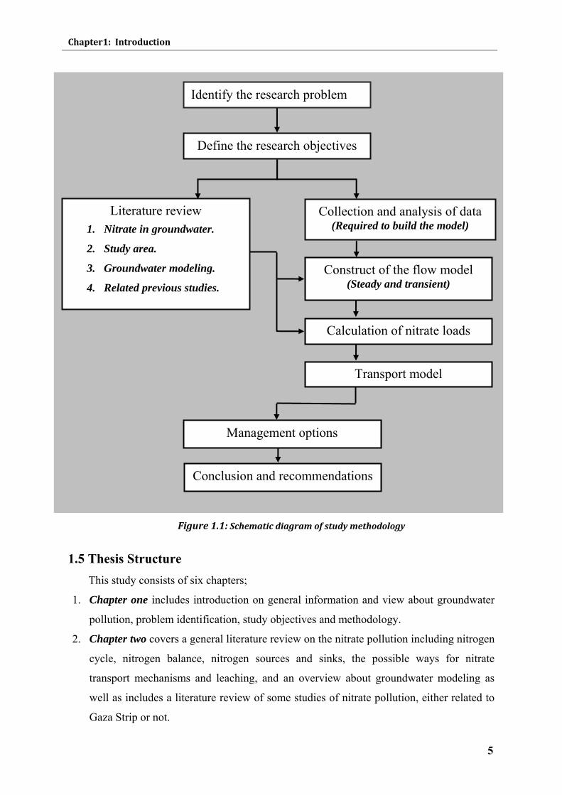
1.4 Methodology The objectives of this research will be achieved by implementing the following steps:
1. Identify the problem of the research and define the objectives.
2. Literature review on the nitrate in groundwater, the study area, groundwater modeling,
and related previous studies.
3. Collection and analysis of the data needed to build the model.
4. Preparation of detailed calculations of nitrate loads in the model area.
5. Develop the conceptual flow and transport model of the study area. Two-stage finite
difference simulation algorithms will be used under steady and transient states for
calibrating the flow and transport parameters.
6. Using the "VMODFLOW Pro" software code to evaluate different management options
or scenarios to improve water quality.
7. Writing the M.Sc thesis which summarizes and reports the achieved results.
Chapter1: Introduction
5
Figure 1.1: Schematic diagram of study methodology
1.5 Thesis Structure This study consists of six chapters;
1. Chapter one includes introduction on general information and view about groundwater
pollution, problem identification, study objectives and methodology.
2. Chapter two covers a general literature review on the nitrate pollution including nitrogen
cycle, nitrogen balance, nitrogen sources and sinks, the possible ways for nitrate
transport mechanisms and leaching, and an overview about groundwater modeling as
well as includes a literature review of some studies of nitrate pollution, either related to
Gaza Strip or not.
Collection and analysis of data (Required to build the model)
Identify the research problem
Define the research objectives
Literature review
1. Nitrate in groundwater.
2. Study area.
3. Groundwater modeling.
4. Related previous studies. Construct of the flow model
(Steady and transient)
Calculation of nitrate loads
Transport model
Management options
Conclusion and recommendations
Chapter1: Introduction
6
3. Chapter three describes the study area with respect to geology, hydro-geology, climate,
Gaza coastal aquifer and water quality of the study area.
4. Chapter four discusses the setting up of the flow and transport models in details. It
presents the steady and transient states flow calibration steps and results to provide the
calibrated parameters.
5. Chapter five covers some of the suggested management scenarios by taking into
consideration the factors affecting the existing and future nitrate contamination of
groundwater.
6. Chapter six contains the conclusion, recommendations, and the limitations of the study.
Note: All calculations of nitrate loads are represented in appendix A.
Chapter2: Literature Review
7
CHAPTER 2
LITERATURE
REVIEW
Chapter2: Literature Review
8
CHAPTER 2: LITERATURE REVIEW
2.1 Nitrate in Groundwater Nitrogen is extremely important to living material. Plants, animals and humans could not
live without it. The major source of nitrogen is the atmosphere. It exists as a colorless,
odorless, nontoxic gas and makes up about 78 % of the atmosphere. Nitrogen is also found in
the Earth's crust as part of organic matter and humus.
The nitrogen gas in our atmosphere exists as a molecule composed of two atoms of
nitrogen. Plants cannot directly use this form of nitrogen. Nitrogen must be converted into
other forms before it can be used by plants. Plant uptake of nitrogen is largely in the form of
nitrate (NO3-), and to a lesser degree ammonium (NH4
+). Nitrogen becomes a concern to water
quality when nitrogen in the soil is converted to the nitrate (NO3-) form. This is because the
nitrate is very mobile and easily moves with water. The concern of nitrates and water quality
is generally directed at groundwater.
Nitrates in the soil result from natural biological processes associated with the
decomposition of plant residues and organic matter. Nitrates can also come from animal
manure, nitrogen fertilizers, and sewage discharges (Killpack and Buchholzfile, 1993).
2.1.1 WHO Standards
Nitrate concentrations are usually expressed in different units, generally of milligrams
per litre (mg/l). The mass representing either the total mass of nitrate ion in the water (nitrate-
NO3-) or only the nitrogen (nitrate-N). The World Health organization recommended
maximum limit for nitrate concentration in drinking water is 11.3 mg/l nitrate-N which is
equivalent to 50 mg/l nitrate-NO3- (WHO, 2003). Water analysis in terms of nitrogen usually
express nitrite (NO2-) and Nitrate (NO3
-) as the total oxidized nitrogen which is the sum of
nitrite and nitrate nitrogen.
2.1.2 The Environmental Health Concerns of Nitrate in Drinking Water
Concentrations of nitrate in groundwater have been known to be a potential human health
problem since Comly (1945) reported that nitrate in drinking water could cause
methaemoglobinemia (Timothy et. al, 2002). The extent of the worldwide problem has been
reviewed by WHO (2003). It has been recommended that water supplies containing high
levels of nitrate (more than 10 mg/l NO3--N) should not be used for the preparation of infant
Chapter2: Literature Review
9
foods, alternative supplies with low nitrate content such using bottled water have been
recommended.
The unsafe levels of nitrate affect the health of people because it associates with gastric
cancer and cause “blue baby” syndrome known as methaemoglobinemia, which can lead to
brain damage and sometimes death (Cabrera and Blarasin, 1999; Lake, 2003; Ramasamy and
Krishnan, 2003).
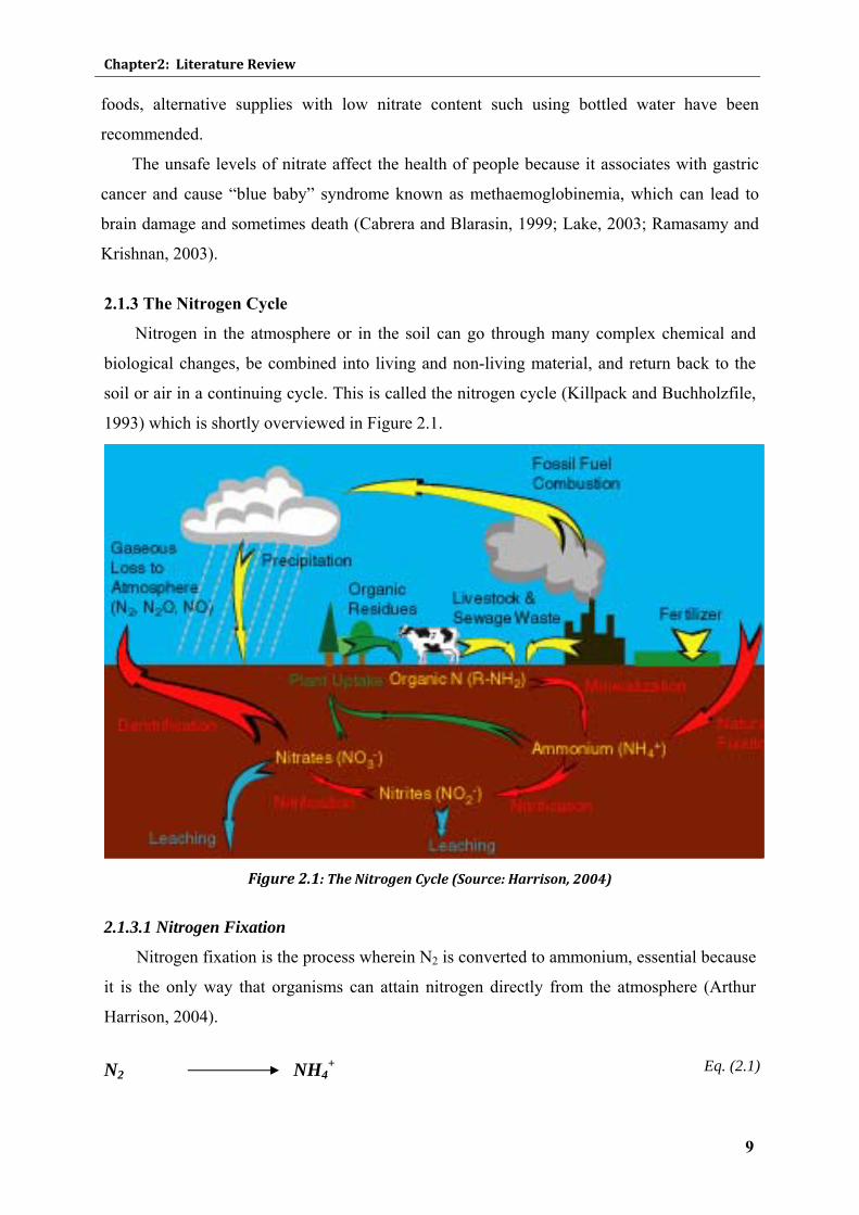
2.1.3 The Nitrogen Cycle
Nitrogen in the atmosphere or in the soil can go through many complex chemical and
biological changes, be combined into living and non-living material, and return back to the
soil or air in a continuing cycle. This is called the nitrogen cycle (Killpack and Buchholzfile,
1993) which is shortly overviewed in Figure 2.1.
Figure 2.1: The Nitrogen Cycle (Source: Harrison, 2004)
2.1.3.1 Nitrogen Fixation
Nitrogen fixation is the process wherein N2 is converted to ammonium, essential because
it is the only way that organisms can attain nitrogen directly from the atmosphere (Arthur
Harrison, 2004).
N2
NH4+
Eq. (2.1)
Chapter2: Literature Review
10
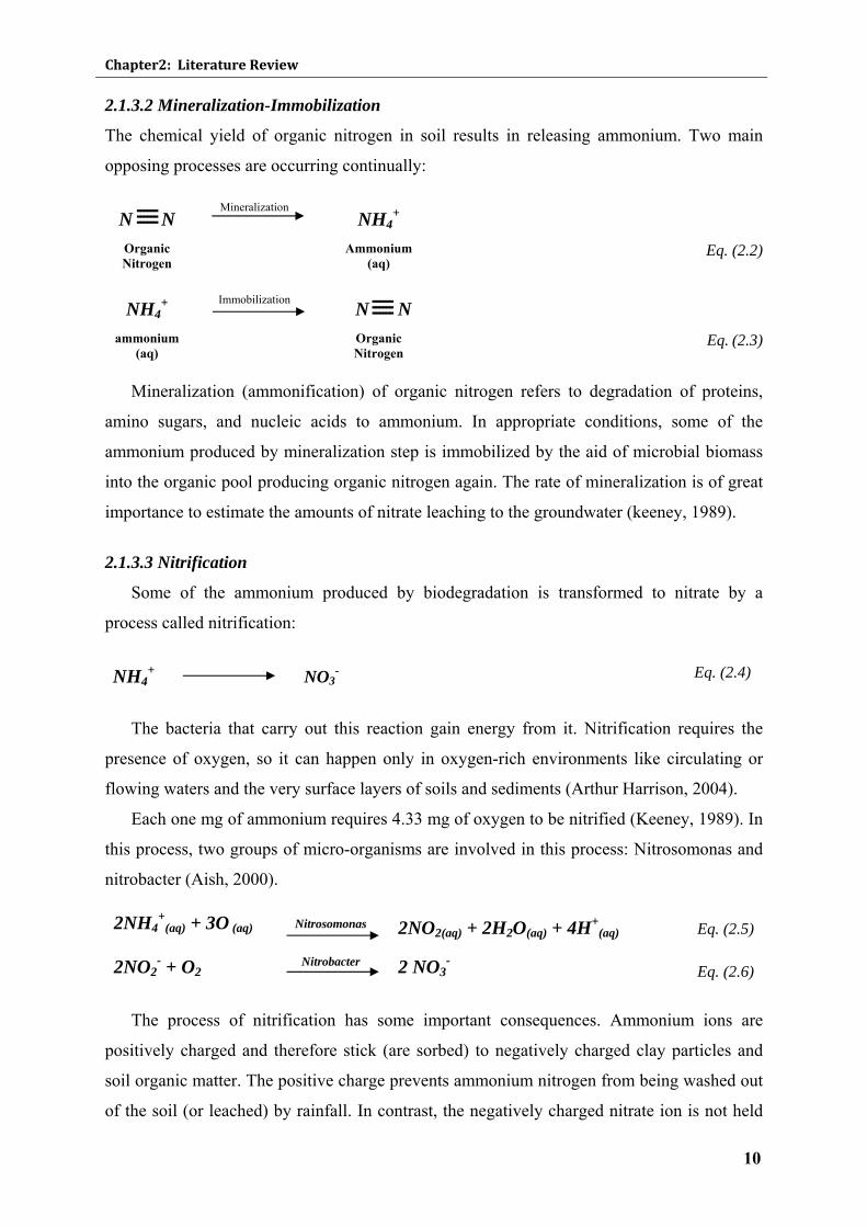
2.1.3.2 Mineralization-Immobilization
The chemical yield of organic nitrogen in soil results in releasing ammonium. Two main
opposing processes are occurring continually:
N N
Mineralization
NH4+
Organic Nitrogen Ammonium
(aq) Eq. (2.2)
NH4+
Immobilization
N N
ammonium (aq) Organic
Nitrogen Eq. (2.3)
Mineralization (ammonification) of organic nitrogen refers to degradation of proteins,
amino sugars, and nucleic acids to ammonium. In appropriate conditions, some of the
ammonium produced by mineralization step is immobilized by the aid of microbial biomass
into the organic pool producing organic nitrogen again. The rate of mineralization is of great
importance to estimate the amounts of nitrate leaching to the groundwater (keeney, 1989).
2.1.3.3 Nitrification
Some of the ammonium produced by biodegradation is transformed to nitrate by a
process called nitrification:
NH4+
NO3-
Eq. (2.4)
The bacteria that carry out this reaction gain energy from it. Nitrification requires the
presence of oxygen, so it can happen only in oxygen-rich environments like circulating or
flowing waters and the very surface layers of soils and sediments (Arthur Harrison, 2004).
Each one mg of ammonium requires 4.33 mg of oxygen to be nitrified (Keeney, 1989). In
this process, two groups of micro-organisms are involved in this process: Nitrosomonas and
nitrobacter (Aish, 2000).
2NH4+
(aq) + 3O (aq)
Nitrosomonas 2NO2(aq) + 2H2O(aq) + 4H+(aq)
Eq. (2.5)
2NO2- + O2
Nitrobacter 2 NO3-
Eq. (2.6)
The process of nitrification has some important consequences. Ammonium ions are
positively charged and therefore stick (are sorbed) to negatively charged clay particles and
soil organic matter. The positive charge prevents ammonium nitrogen from being washed out
of the soil (or leached) by rainfall. In contrast, the negatively charged nitrate ion is not held
ــــــ ــــــ ــــــ
ــــــ ــــــ ــــــ
Chapter2: Literature Review
11
by soil particles and so can be washed down the soil profile, leading to decreased soil fertility
and nitrate enrichment of downstream surface and groundwater. (Arthur Harrison, 2004)
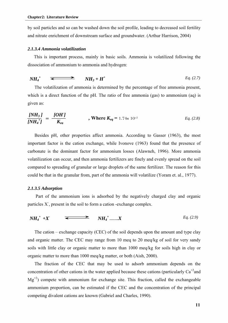
2.1.3.4 Ammonia volatilization
This is important process, mainly in basic soils. Ammonia is volatilized following the
dissociation of ammonium to ammonia and hydrogen:
NH4+
NH3 + H+
Eq. (2.7)
The volatilization of ammonia is determined by the percentage of free ammonia present,
which is a direct function of the pH. The ratio of free ammonia (gas) to ammonium (aq) is
given as:
, Where Keq = 1.74x 10⁻⁵ Eq. (2.8)
Besides pH, other properties affect ammonia. According to Gasser (1963), the most
important factor is the cation exchange, while Ivonove (1963) found that the presence of
carbonate is the dominant factor for ammonium losses (Alawneh, 1996). More ammonia
volatilization can occur, and then ammonia fertilizers are finely and evenly spread on the soil
compared to spreading of granular or large droplets of the same fertilizer. The reason for this
could be that in the granular from, part of the ammonia will volatilize (Yoram et. al., 1977).
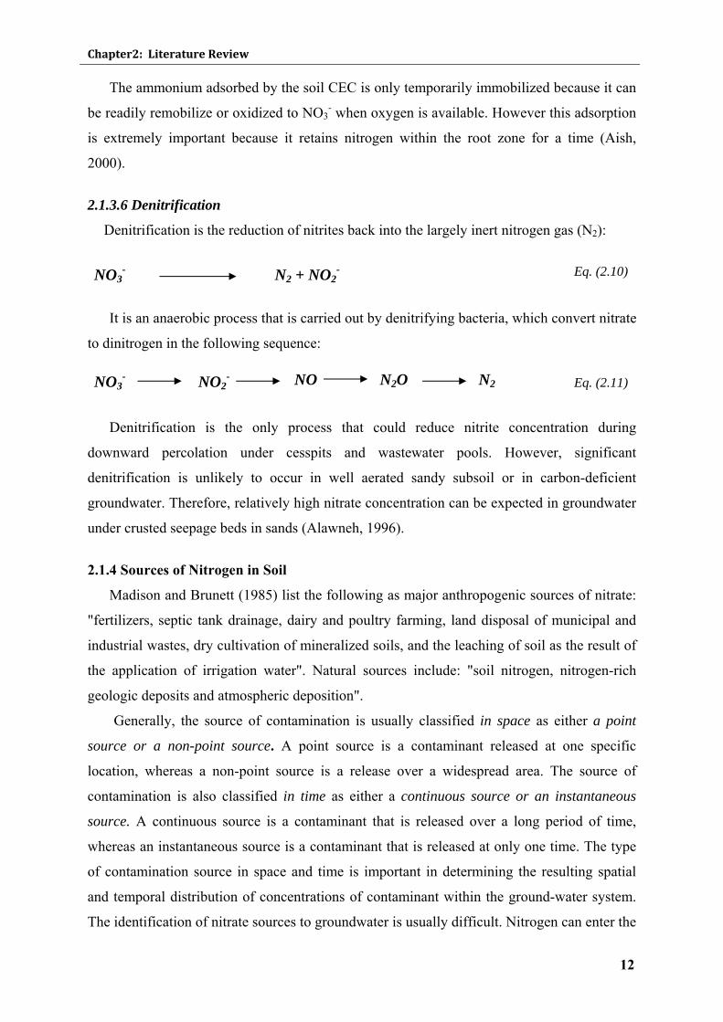
2.1.3.5 Adsorption
Part of the ammonium ions is adsorbed by the negatively charged clay and organic
particles X-, present in the soil to form a cation -exchange complex.
NH4+ +X-
NH4+ …….X
Eq. (2.9)
The cation – exchange capacity (CEC) of the soil depends upon the amount and type clay
and organic matter. The CEC may range from 10 meq to 20 meq/kg of soil for very sandy
soils with little clay or organic matter to more than 1000 meq/kg for soils high in clay or
organic matter to more than 1000 meq/kg matter, or both (Aish, 2000).
The fraction of the CEC that may be used to adsorb ammonium depends on the
concentration of other cations in the water applied because these cations (particularly Ca+2and
Mg+2) compete with ammonium for exchange site. This fraction, called the exchangeable
ammonium proportion, can be estimated if the CEC and the concentration of the principal
competing divalent cations are known (Gabriel and Charles, 1990).
[NH3 ] [OH-]
[NH4+] Keq
=
Chapter2: Literature Review
12
The ammonium adsorbed by the soil CEC is only temporarily immobilized because it can
be readily remobilize or oxidized to NO3- when oxygen is available. However this adsorption
is extremely important because it retains nitrogen within the root zone for a time (Aish,
2000).
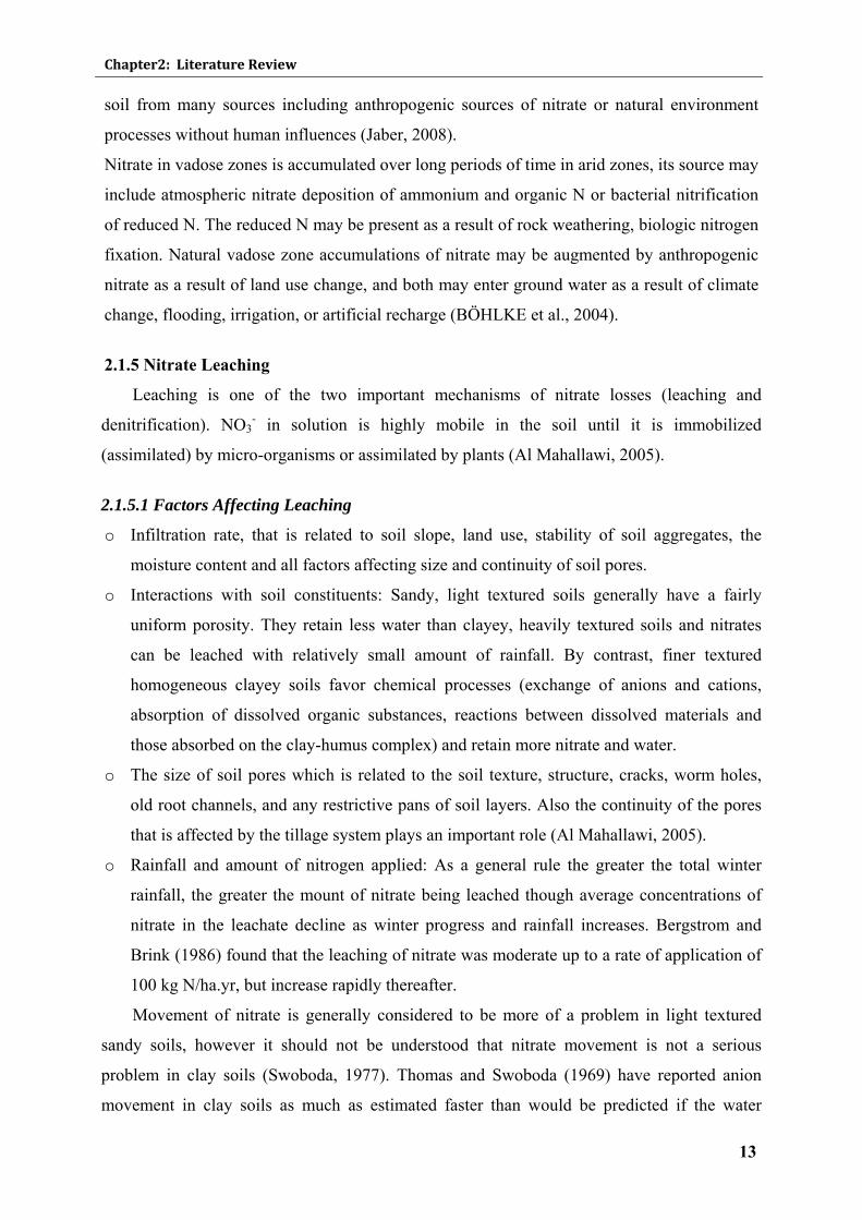
2.1.3.6 Denitrification
Denitrification is the reduction of nitrites back into the largely inert nitrogen gas (N2):
NO3-
N2 + NO2-
Eq. (2.10)
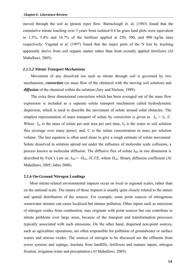
It is an anaerobic process that is carried out by denitrifying bacteria, which convert nitrate
to dinitrogen in the following sequence:
NO3- NO2
-
NO N2O N2 Eq. (2.11)
Denitrification is the only process that could reduce nitrite concentration during
downward percolation under cesspits and wastewater pools. However, significant
denitrification is unlikely to occur in well aerated sandy subsoil or in carbon-deficient
groundwater. Therefore, relatively high nitrate concentration can be expected in groundwater
under crusted seepage beds in sands (Alawneh, 1996).
2.1.4 Sources of Nitrogen in Soil
Madison and Brunett (1985) list the following as major anthropogenic sources of nitrate:
"fertilizers, septic tank drainage, dairy and poultry farming, land disposal of municipal and
industrial wastes, dry cultivation of mineralized soils, and the leaching of soil as the result of
the application of irrigation water". Natural sources include: "soil nitrogen, nitrogen-rich
geologic deposits and atmospheric deposition".
Generally, the source of contamination is usually classified in space as either a point
source or a non-point source. A point source is a contaminant released at one specific
location, whereas a non-point source is a release over a widespread area. The source of
contamination is also classified in time as either a continuous source or an instantaneous
source. A continuous source is a contaminant that is released over a long period of time,
whereas an instantaneous source is a contaminant that is released at only one time. The type
of contamination source in space and time is important in determining the resulting spatial
and temporal distribution of concentrations of contaminant within the ground-water system.
The identification of nitrate sources to groundwater is usually difficult. Nitrogen can enter the
Chapter2: Literature Review
13
soil from many sources including anthropogenic sources of nitrate or natural environment
processes without human influences (Jaber, 2008).
Nitrate in vadose zones is accumulated over long periods of time in arid zones, its source may
include atmospheric nitrate deposition of ammonium and organic N or bacterial nitrification
of reduced N. The reduced N may be present as a result of rock weathering, biologic nitrogen
fixation. Natural vadose zone accumulations of nitrate may be augmented by anthropogenic
nitrate as a result of land use change, and both may enter ground water as a result of climate
change, flooding, irrigation, or artificial recharge (BÖHLKE et al., 2004).
2.1.5 Nitrate Leaching
Leaching is one of the two important mechanisms of nitrate losses (leaching and
denitrification). NO3- in solution is highly mobile in the soil until it is immobilized
(assimilated) by micro-organisms or assimilated by plants (Al Mahallawi, 2005).
2.1.5.1 Factors Affecting Leaching
o Infiltration rate, that is related to soil slope, land use, stability of soil aggregates, the
moisture content and all factors affecting size and continuity of soil pores.
o Interactions with soil constituents: Sandy, light textured soils generally have a fairly
uniform porosity. They retain less water than clayey, heavily textured soils and nitrates
can be leached with relatively small amount of rainfall. By contrast, finer textured
homogeneous clayey soils favor chemical processes (exchange of anions and cations,
absorption of dissolved organic substances, reactions between dissolved materials and
those absorbed on the clay-humus complex) and retain more nitrate and water.
o The size of soil pores which is related to the soil texture, structure, cracks, worm holes,
old root channels, and any restrictive pans of soil layers. Also the continuity of the pores
that is affected by the tillage system plays an important role (Al Mahallawi, 2005).
o Rainfall and amount of nitrogen applied: As a general rule the greater the total winter
rainfall, the greater the mount of nitrate being leached though average concentrations of
nitrate in the leachate decline as winter progress and rainfall increases. Bergstrom and
Brink (1986) found that the leaching of nitrate was moderate up to a rate of application of
100 kg N/ha.yr, but increase rapidly thereafter.
Movement of nitrate is generally considered to be more of a problem in light textured
sandy soils, however it should not be understood that nitrate movement is not a serious
problem in clay soils (Swoboda, 1977). Thomas and Swoboda (1969) have reported anion
movement in clay soils as much as estimated faster than would be predicted if the water
Chapter2: Literature Review
14
moved through the soil as (piston type) flow. Barraclough et. al. (1983) found that the
cumulative nitrate leaching over 3 years from isolated 0.4 ha grass land plots were equivalent
to 1.5%, 5.4% and 16.7% of the fertilizer applied at 250, 500, and 900 kg/ha rates
respectively. Vagstad et al. (1997) found that the major parts of the N lost by leaching
apparently derive from soil organic matter rather than from recently applied fertilizers (Al
Mahallawi, 2005).
2.1.5.2 Nitrate Transport Mechanisms
Movement of any dissolved ion such as nitrate through soil is governed by two
mechanisms, convection (or mass flow of the chemical with the moving soil solution) and
diffusion of the chemical within the solution (Jury and Nielsen, 1989).
The extra three dimensional convection which has been averaged out of the mass flow
expression is included as a separate solute transport mechanism called hydrodynamic
dispersion, which is used to describe the movement of solute around solid obstacles. The
simplest representation of mass transport of solute by convection is given as Jsc = Jw .C.
Where Jsc is the mass of solute per unit area per unit time, Jw is the water or soil solution
flux (average over many pores), and, C is the solute concentration in mass per solution
volume. The last equation is often used alone to give a rough estimate of solute movement.
Solute dissolved in solution spread out under the influence of molecular scale collisions, a
process known as molecular diffusion. The diffusive flux of solute JSD in one dimension is
described by Fick’s Law as: JSD = -Dsw. ∂C/∂Z, where Dsw: Binary diffusion coefficient (Al
Mahallawi, 2005; Jaber 2008).
2.1.6 On-Ground Nitrogen Loadings
Most nitrate-related environmental impacts occur on local or regional scales, rather than
on the national scale. The nature of those impacts is usually quite closely related to the nature
and spatial distribution of the sources. For example, some point sources of nitrogenous
wastewater streams can cause localized but intense pollution. Other inputs such as emissions
of nitrogen oxides from combustion, may originate with point sources but can contribute to
nitrate problems over large areas, because of the transport and transformation processes
typically associated with such emissions. On the other hand, dispersed non-point sources,
such as agriculture operations, are often responsible for pollution of groundwater or surface
waters and nitrous oxides. The sources of nitrogen to be discussed are the effluents from
sewer systems and septage, leachate from landfills, fertilizers and manure inputs, nitrogen
fixation, irrigation water and precipitation (Al Mahallawi, 2005).
Chapter2: Literature Review
15
2.1.6.1 Effluent from sewer systems and septage
Untreated sewage flowing from municipal collection systems typically contains 20-85
mg/l total nitrogen (Scheible, 1994). The total nitrogen in domestic sewage comprises
approximately 60% ammonia nitrogen, 40% organic nitrogen and very small quantities of
nitrates. The septage from rural areas has a nitrogen content of 100-1600 mg/l TKN (Total
Kjeldahl Nitrogen) with 700 mg/l TKN typical value (Metcalf and Eddy, 1990). At least half
of the nitrogen that enters sewage treatment facilities is not removed, and is discharged in the
environment largely as ammonia or nitrate (National Academy of Science, 1978).
Magdoff and Keeny, (1976) found that the removal of nitrogen in the septage by soil
materials is nearly about 22%. This makes septage a major local source of nitrate. Significant
denitrification is not likely if seepage for the effluent is built in deep sandy soils (Walker et
al., 1973a). In the movement of nitrate through sand soil beneath a septic tank disposal field;
nitrate concentration increased, and ammonia concentration decreased with depth. Walker et
al. (1973b) reported nitrate concentrations from 2 to 42 mg/L in groundwater around several
non-sewered households in a sandy soil area of central Wisconsin; the highest concentrations
were just down the flow gradient from the disposal field. As distance from the septic tank
field increased, nitrate concentrations declined rapidly because of dilution groundwater.
Contamination of groundwater by nitrate from septic tanks and cesspits is of little
significance in sparsely population rural areas; however increased population density can
produce high nitrate levels in groundwater supplies (Al Mahallawi, 2005).
2.1.6.2 Leachate From landfills Leachate from municipal solid waste landfills is characterized as a relatively low volume,
high-strength wastewater. A survey of leachate characterized for many landfills shows
ammonium values of 0–1160 mg/l and nitrate plus nitrite nitrogen of 0.2–10.2 mg/l (Scheible,
1994). Depending on the landfill and the materials placed in it, typical values of nitrogen in
the landfill leachate are 200 mg/l organic nitrogen, 200 mg/l ammonia nitrogen and 25 mg/l
nitrate nitrogen (Rabah, 1997).
Poul et al.1995, found that the leachate of the Grindsted landfill in Denmark contains
lower ammonium concentration closer to the landfill and they related this to the cation
exchange process that may attenuate ammonium in the anaerobic part of the plume. The
leakage of organic and inorganic pollutants from old landfills without leachate collecting
system may influence the groundwater quality and thereby be a risk for drinking water. The
composition of leachate from landfills is dependent on the age of the landfill (Al Mahallawi,
2005).
Chapter2: Literature Review
16
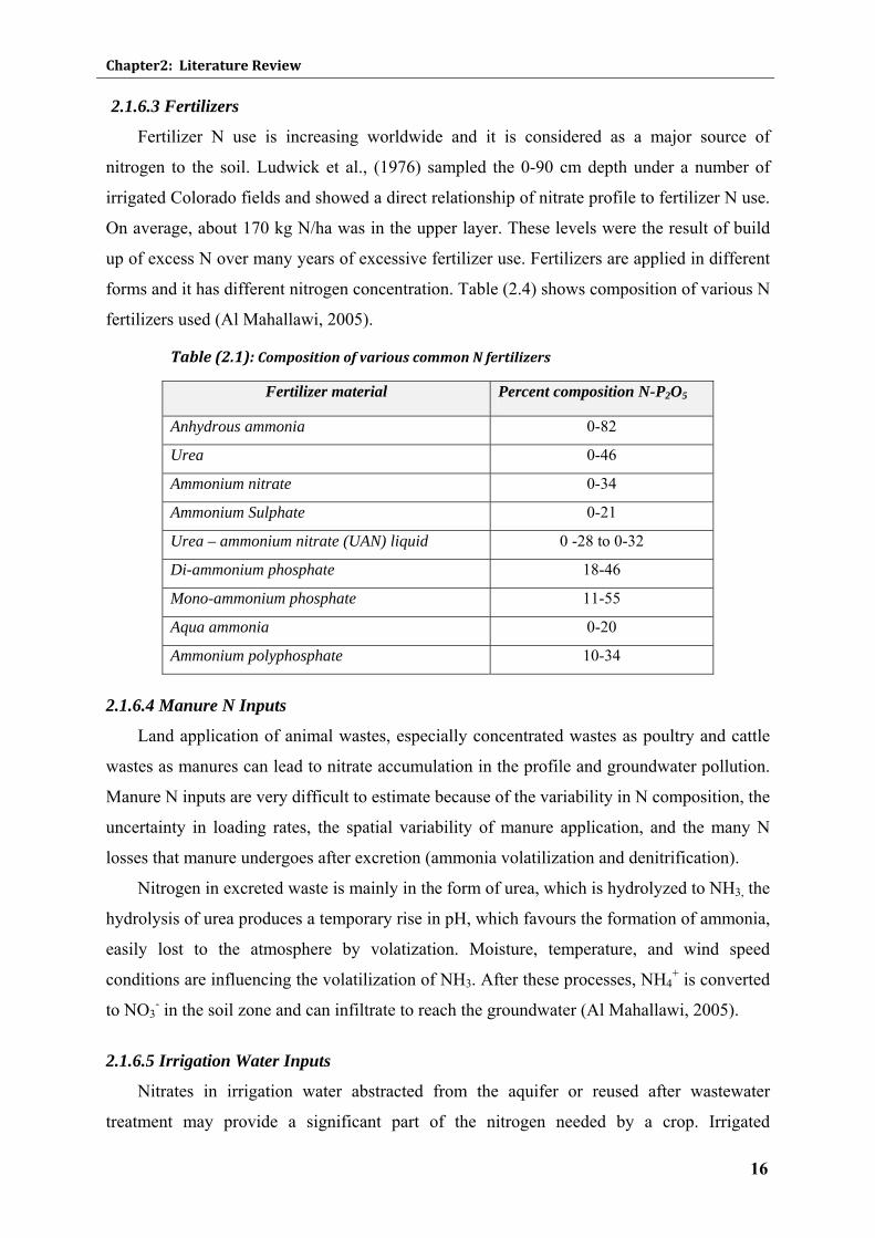
2.1.6.3 Fertilizers
Fertilizer N use is increasing worldwide and it is considered as a major source of
nitrogen to the soil. Ludwick et al., (1976) sampled the 0-90 cm depth under a number of
irrigated Colorado fields and showed a direct relationship of nitrate profile to fertilizer N use.
On average, about 170 kg N/ha was in the upper layer. These levels were the result of build
up of excess N over many years of excessive fertilizer use. Fertilizers are applied in different
forms and it has different nitrogen concentration. Table (2.4) shows composition of various N
fertilizers used (Al Mahallawi, 2005).
Table (2.1): Composition of various common N fertilizers
Fertilizer material Percent composition N-P2O5
Anhydrous ammonia 0-82
Urea 0-46
Ammonium nitrate 0-34
Ammonium Sulphate 0-21
Urea – ammonium nitrate (UAN) liquid 0 -28 to 0-32
Di-ammonium phosphate 18-46
Mono-ammonium phosphate 11-55
Aqua ammonia 0-20
Ammonium polyphosphate 10-34
2.1.6.4 Manure N Inputs
Land application of animal wastes, especially concentrated wastes as poultry and cattle
wastes as manures can lead to nitrate accumulation in the profile and groundwater pollution.
Manure N inputs are very difficult to estimate because of the variability in N composition, the
uncertainty in loading rates, the spatial variability of manure application, and the many N
losses that manure undergoes after excretion (ammonia volatilization and denitrification).
Nitrogen in excreted waste is mainly in the form of urea, which is hydrolyzed to NH3, the
hydrolysis of urea produces a temporary rise in pH, which favours the formation of ammonia,
easily lost to the atmosphere by volatization. Moisture, temperature, and wind speed
conditions are influencing the volatilization of NH3. After these processes, NH4+ is converted
to NO3- in the soil zone and can infiltrate to reach the groundwater (Al Mahallawi, 2005).
2.1.6.5 Irrigation Water Inputs
Nitrates in irrigation water abstracted from the aquifer or reused after wastewater
treatment may provide a significant part of the nitrogen needed by a crop. Irrigated
Chapter2: Literature Review
17
agriculture is a primary source of nitrate. The inputs can be readily estimated from the
quantity of water applied and its N content (Al Mahallawi, 2005; Jaber, 2008).
2.1.6.6 Nitrogen Fixation Inputs
The N2 fixation converts atmospheric N2 gas into plant N through bacteria living in root
nodules of certain plants, primarily legumes. The mass of fixed N depends on many
environmental factors including plant species, available soil N, crop management, soil water,
type of fixing bacteria and soil chemical environment. Nitrogen fixation is an adaptive
process that occurs at significant rates only when the supply of fixed nitrogen is low and
apparently growth-limiting. Fixation of nitrogen requires a considerable input of energy. The
estimates of nitrogen fixation will be rather crude (Al Mahallawi, 2005; Jaber, 2008).
2.1.6.7 Precipitation Inputs
The atmosphere contains ammonia and compounds released from soil and plants as well
as from the combustion of coal and petroleum products. The main sources of atmospheric N
are combustion of fuels, volatilization of NH3 from animal wastes and fertilizers, volcanoes,
and lightening. The principal forms of N in precipitation are NH3, N-oxides and organic N.
The concentration of nitrogen in precipitation in most cases will contain between 1 and 4
mg/l total N (Al Mahallawi, 2005).
2.1.7 Losses of Nitrogen
The main losses of nitrogen are ammonia volatilization, denitrification, plant uptake,
leaching (leaching was discussed before), erosion and runoff.
2.1.7.1 Losses Through Ammonia Volatilization
Ammonia volatilization is a complex process involving chemical and biological
reactions within the soil, and physical transport of N out of the soil. The most favourable
conditions for ammonia losses to occur are N sources containing urea, fertilizers application
in surface, soil pH above 7, and dry weather conditions. The intensity of ammonia
volatilization from solution is directly related to the concentration of dissolved ammonia in
the water. Ammonia volatilization from acidic solutions is negligible. Ammonia volatilization
fellows first order reaction kinetics. The rate of volatilization is severely restricted by limiting
the movement of air above the water, enhanced by water turbulence and increased
exponentially with temperature. pH of the solution is the dominant factor controlling the
extent of ammonia volatilization when the concentration of ammonium in the soil is low. At
high pH and high initial ammonium concentrations, the dominant factor controlling the
Chapter2: Literature Review
18
reaction is the buffer capacity of the soil. Losses from unincorporated surface application of
NH4+ sources on high pH soils or urea-containing sources on any soil can reach as high as
30% to 50%.
2.1.7.2 Losses Through Denitrification
Biological denitrification is the main method of removing nitrogen because it returns
nitrogen to the atmosphere as inert N2 gas and complete the nitrogen cycle. Several
intermediates are involved as: NO3- NO2
- NO N2O N2 (gas).
E. coli is one of the organisms which converts nitrate to nitrite under anaerobic
conditions, and does not do the subsequent reaction steps. It utilizes the best available
electron acceptor available, i.e. nitrate. Bacteria of facultative anaerobes normally used
oxygen of the air as hydrogen acceptor (aerobically) but also possess the ability to use
nitrates and nitrites in the place of oxygen anaerobically and predominantly in two genera:
Pseudomonas and Bacillus. Many soil bacteria like Thiobacillus also reduce nitrate to
nitrogen. The anaerobic conversion of nitrate into molecular of nitrogen is also known as
nitrate respiration. It is likely to be found in agricultural land receiving substantial inputs of
nitrogenous fertilizers or manure. The common requirements for denitrification are;
• The presence of an electron acceptor which in this case is nitrate,
• Presence of a microbial population that possess the metabolic capacity. Researches has
shown that denitrification losses are higher in manured soils than the non-manured soils,
• Presence of suitable electron donors and,
• The presence of anaerobic conditions or restricted oxygen availability.
The main limiting condition for these four conditions is the presence of dissolved
oxygen, which is highly observed in shallow depths. So, nitrate is most likely to be denitrified
at deep depths due to lack of oxygen (Almasri and Kaluarachchi, 2004). Their study about
Whatcom County, Washington, recognized by heavy agricultural activities, shows the
relationship between the nitrate concentration and dissolved oxygen concentration. High
nitrate concentrations are noticed at high dissolved oxygen concentrations and vice versa
(Jaber, 2008).
2.1.7.3 Plant Uptake
The amount of N consumed by plants varies greatly from one species to another and for
any given species; the amount varies with the environment. Also considerable variation exists
in the relative amount of the N contained in the different plant parts. Substantial variation can
Chapter2: Literature Review
19
occur depending on soil N status, fertilization management, and climate. Nitrogen uptake by
plants is very rapid during the period of rapid vegetative growth (Jaber, 2008).
2.1.7.4 Erosion and runoff
Nitrogen losses in surface runoff (that is dissolved in the runoff water) are usually small.
Such losses are variable however and depend on degree of soil cover, source of N applied,
rainfall intensity immediately after application, and soil properties such as soil crusting. The
largest losses (e.g., 10% losses) occur if a soluble N source is surface applied to a bare soil
and significant runoff events occur within one day of application. In most cases, runoff N
losses are small and may reach 3 kg/ha annually or less (Legg and Meisinger, 1982).
2.2 Groundwater Modeling
A groundwater model is a representation of reality and, if properly constructed, it can be
a valuable predictive tool used for management of groundwater resources (Wang and
Anderson, 1982). A mathematical model simulates groundwater flow indirectly by means of
governing equation that represents the physical processes that occur in the system, together
with equations that describe heads or flows along the boundaries of the model.
For time-dependent problems, an equation describing the initial distribution of heads in
the system is also needed (Anderson and Woessner, 1992).
2.2.1 General Groundwater Flow Equations
Differential equations that govern the flow of groundwater flow can essentially represent
the groundwater flow system derived from the basic principles of groundwater flow
hydraulics. The main flow equation for saturated groundwater flow is derived by combining a
water balance equation with Darcy’s law, which leads to a general form of the 3-D
groundwater flow governing equation:
thSw
zhK
zyhK
yxhK
x szyx ∂∂
=+⎟⎠⎞
⎜⎝⎛
∂∂
∂∂
+⎟⎟⎠
⎞⎜⎜⎝
⎛∂∂
∂∂
+⎟⎠⎞
⎜⎝⎛
∂∂
∂∂
Eq. (2.12)
Where Kx, Ky and Kz are the hydraulic conductivity components in the x, y and z
direction (LT-1), h is the hydraulic head (L), w is the local source or sink of water per unit
volume (T-1 ), Ss is the specific storage coefficient (L-1) and t is the time ( T ). Under steady
state conditions, Eq. (2.12) is equal to zero as continuity requires that the amount of water
flowing in to a representative elemental volume is equal to the amount flowing out, this leads
to Eq. (2.13):
Chapter2: Literature Review
20
0=+⎟⎠⎞
⎜⎝⎛
∂∂
∂∂
+⎟⎟⎠
⎞⎜⎜⎝
⎛∂∂
∂∂
+⎟⎠⎞
⎜⎝⎛
∂∂
∂∂ w
zhK
zyhK
yxhK
x zyx Eq. (2.13)
In transient conditions the general flow equation is formulated by applying the law of
conservation of mass over an elemental volume of an aquifer situated in the flow field in
function of time. Continuity requires that the net inflow into the elemental control volume
must be equal to the rate at which water is accumulating within the volume under
investigation, which is outflow minus inflow equals change in storage. The change in storage
is represented by the specific storage, or specific storage coefficient, Ss, which is defined as
the volume of water released from storage per volume of soil for a unit decline in hydraulic
head (Aish 2004; Jaber 2008).
2.2.2 Numerical Methods of Solving Flow Equations
Groundwater flow equations are usually not easy to solve analytically. This is because
either the flow is described by a partial differential equation or usually the medium properties
are heterogeneous. In such cases, numerical solution techniques can be used to obtain
approximations.
Two major classes of numerical methods have been accepted for solving the
groundwater flow equation. These are finite difference methods and finite element methods.
Finite difference method is much easier in programming and application than finite
element method in which the heads at the nodes can be computed as an average value of the
cells surrounding the node. However, finite element method is suitable for irregular shaped
boundaries because the variations of heads within the element can be handled by means of an
interpolation function, so it can handle complex geometry and important parameters with
high accuracy (Aish 2004; Jaber 2008).
2.2.3 Solute Transport
Advection is the primary transport mechanism by which a pollutant can be transported
through a groundwater system, which is the movement of a dissolved chemical along with the
groundwater flow. In addition to transport by advection, dissolved particles are also subjected
to hydrodynamic dispersion, a process accounting for the seemingly random spreading of
solutes. Dispersion causes particles to deviate from the macroscopic advective flow paths that
do not take into account the actual geometry of the pore space. Hence, some particles will
move faster and some slower due to the difference in size of the pores, while also deviations
in direction of the flow will because the particles have to move around the solid material. The
resulting dispersion is rather random and as such very similar to diffusive spreading, but
Chapter2: Literature Review
21
generally it has a much wider impact on the transport of dissolved chemicals compared to
diffusion. In addition to transport by advection and dispersion, other processes can affect the
transport of solutes, as adsorption of chemicals on the solid material of the porous medium.
The partial differential equation describing the fate and transport of contaminants of species k
in 3-D, transient ground water flow systems can be written as following (Zheng and Wang,
1999):
( ) ( ) ∑++∂∂
−⎟⎟⎠
⎞⎜⎜⎝
⎛
∂∂
∂∂
=∂
∂n
kss
ki
ij
k
iji
k
RCqCvxx
CDxt
C θθθ Eq. (2.14)
Where,
- θ is porosity of the subsurface medium, dimensionless;
- Ck is dissolved concentration of species k (M L-3);
- t is time (T);
- xi,,j is distance along the respective Cartesian coordinate axis (L);
- Dij is hydrodynamic dispersion and diffusion coefficient tensor (L2 T-1);
- vi is seepage or linear pore water velocity (L T-1); it is related to the specific discharge or
Darcy flux through the relationship, vi = qi/θ ;
- qs is volumetric flow rate per unit volume of aquifer representing fluid sources (positive)
and sinks (negative) (T-1); - Ck
s is concentration of the source or sink flux for species k (M L-3);
- Rn is chemical reaction term (M L-3 T-1).
2.2.4 Numerical Methods of Solute Transport Equations
The numerical solutions for solute transport are different and rather difficult. This
difficulty is essentially due to the advective component of solute transport. Three main
methods are used for solving the solute transport equation; method of characteristic (MOC),
modified method of characteristics (MMOC) and hybrid method of characteristics (HMOC).
• The Method Of Characteristic (MOC)
The method of characteristic consists of computing the advective term of the transport
equation, using moving particles that represent the solute concentrations. A set of particles is
assigned; each particle has the concentration of the cell where it is located. Then, if only the
advective effect is assumed, the concentrations will travel through the flow paths since the
advective term is proportional to the velocity vector. Hence, the concentrations will be
estimated by a forward particle tracking method. Then having the advective term, these
Chapter2: Literature Review
22
concentrations are injected into the dispersion, sink/sources and chemical reaction terms and
solved by Eulerian method, with finite-difference or finite-elements.
• Modified Method Of Characteristics (MMOC)
The modified method of characteristics was originally developed to approximate the
advection term, but the particles are assigned to fixed coordinates that are the grid nodes and
the tracking is no more forward, but rather backward. For each particle, that has the node
position, the preceding position (corresponding to time step n-1) is calculated from the
present time step n. Assigning immobile coordinates for the particles at each time step saves a
lot of time processing and computer storage. Hence, the modified method of characteristic
reduces dramatically the time consuming in the solute transport equation solution. However,
the advantage of saving huge computer memory is balanced by numerical problems in zones
where sharp fronts of solute concentration are present.
• Hybrid Method of Characteristics (HMOC)
The two previous methods have shown their limitations when applied to solute transport
equations. As a matter of fact, to take advantage of the MOC and MMOC, a concept of
combining these two methods was developed, and characterized as HMOC. This method
consists of using the method of characteristic when sharp fronts of solute exist, while away
from those zones the modified method of characteristic is used. An automatic choice of the
method is based on the solute concentration distribution during the time period, and after
each time step (Aish 2004; Jaber 2008).
2.3 Related Studies Many studies were performed on water quality of the Gaza Strip aquifer in related with
increase of nitrate pollution, a lot of them focused on the relationship between land use and
groundwater contamination by nitrate. This section contains a brief explanation to the
findings of the previous studies ordered from oldest to newest. 1. In 1995, a study about nitrate pollution in Gaza groundwater was done by the
Environmental Planning Directorate in the Ministry of Planning in Gaza (Maarten
Gischler, 1997). They followed an approach of nitrogen balances. In urban areas they
calculated an N-load per ha based on population density, daily N-production per
capita, percentage of population sewered, and assuming a certain removal coefficient
to account for volatilization of NH3, ammonium adsorption and many other factors.
Hading calculated this load for each city; the N-load was dissolved to the amount of
recharge percolating to the groundwater. They compared this with nitrogen
concentration and found a remarkable correlation or good relationship. In agricultural
Chapter2: Literature Review
23
areas, they followed a similar approach and found that nitrogen applied through
fertilizers is in some crops more than ten times the potential plant uptake. This
explained the great jump of nitrate concentrations over the last years. However,
dissolving the N-load in the amount of recharge did not give a very good correlation
with nitrate concentrations found in the groundwater.
2. In 1997, a study of title "Quantification of nitrate pollution to groundwater resources
of Rafah (Gaza Strip)" was done by Dr. Fahed Rabah as a M.Sc Thesis in IHE, Delft,
the Netherlands. This study is devoted for the investigation of the sources of nitrate
pollution to groundwater in Rafah and the assessment of the contribution of each
source to the pollution load. Through field word investigations it has been found that
agricultural and urban activities are the two major nitrate sources in Rafah.
Agricultural activity contribution to nitrate pollution is investigated through N-
balance for most of the crops cultivated in Rafah. The produced nitrate leachate under
different crops is estimated and found to be in the range of 300-1900 mg No3 /L.
Urban activity contribution to nitrate pollution is also investigated through N-balance
for different locations in Rafah. The produced nitrate leachate under different urban
pollution sources (cesspits, solid waste, overflow ponds ….etc) is estimated to be in
the range of 250-2000 mg No3 /L. The relation between the nitrate in the leachate of
the pollution sources and that in the groundwater is assessed by a set of expected
scenarios which confirmed that the nitrate pollution to groundwater of Rafah is a
human-made pollution through agricultural and urban activities while natural nitrate
sources are of negligible effect.
3. In 2002, Molenat and Gascuel-Odoux developed a two dimensional model to
characterize the flow and nitrate transport in the groundwater within a hillslope of the
Kervidy catchments in France. The finite-difference code MODFLOW was used to
simulate the distribution of hydraulic head within the groundwater. Nitrate transport
was described by the convection equation solved using MT3D. MODPATH was also
used to analyze flow paths and travel times in the groundwater. Autotrophic and
heterotrophic denitrification in the soil was represented. A steady-state average flow
was assumed with a spatially uniform groundwater recharge found in the study area.
Nitrate recharge rate was fixed at 100 mg/l, equivalent to a nitrogen flux of 165
kg/ha/year. Six scenarios of nitrate leaching changes were analyzed using the model.
The first two correspond to spatially uniform decreases of the nitrate recharge rate to
80 and 60 mg/l respectively. In the other four scenarios, nitrate recharge rate was
Chapter2: Literature Review
24
spatially distributed along the study area while the average nitrogen flux remained
equal to 165 kg/ha/year. The transport model reproduced the spatial pattern of nitrate
concentrations observed in the groundwater. Scenarios analysis showed that a
significant decrease of stream nitrate concentration could be expected following a
global decrease in nitrate leaching along the hillslope and the fall could be very
gradual in time.
4. In 2004, a study about "Seasonal variations and mechanisms of groundwater nitrate
pollution in the Gaza Strip" was performed by Y. Abu Maila, I. El-Nahal and
M. R. Al-Agha. This study showed that nitrate is one of the major pollutants of
groundwater in the Gaza Strip. Several cases of blue babies disease were reported in
the last couple of years. The average concentration of nitrate in domestic wells is
128 mg/L in June-July and 118 mg/L in Jan-Feb, and for the agricultural wells, the
average is 100 mg/L in June-July and 96 mg/L for Jan-Feb. The results suggest that
the seasonal differences in nitrate concentrations of the domestic wells are slightly
more observable than those of the agricultural wells. The environmental factors that
control nitrate in groundwater are: a partially-confined aquifer, lack of a sewage
system, population density, the presence of refugee camps, the presence of fertilizers
and the annual rain. The variations in nitrate concentration of the domestic wells are
not of considerable values. It is suggested that concrete policies in pollution control
and/or prevention measures could be formulated upon better understanding of the
environmental factors.
5. In 2005, Chowdary et al. developed a groundwater flow and solute transport model to
assess the impacts of non-point-source pollution from fertilizers on groundwater
quality in the aquifers underlying the Godavari Delta Central Canal, India. The model
involved five steps or processes combining the variation in weather, crop, soil, water
supplies, fertilizers use, and environment interactions; 1) Recharge of groundwater by
seepage from water distribution network, 2) Recharge of groundwater by percolation
from fields in the study area estimated by soil water balance model constructed by
Chowdary et al., accounted the important nitrogen transformations adopted for the
study, 3) The concentration of nitrates in the percolated water out of the root zone was
governed by the nitrogen balance to determine the nitrate pollutant loads from applied
fertilizers. Chowdary et al. modeled the transport and transformations of different N
species in the soil, water, plant, and atmosphere system, taking into consideration the
main processes including hydrolysis, ammonia volatilization, mineralization and
Chapter2: Literature Review
25
immobilization, nitrification, denitrification, leaching and plant uptake, 4)
Groundwater flow in the aquifer underlying the project area in response to recharge,
and 5) Transport of nitrates in the aquifer; Geographic Information System (GIS)
tools were used to represent the input data and map the output of the recharge,
nitrogen balance and loading. Alternative strategies of resource management were
evaluated to minimize the impacts.
6. Al Mahallawi (2005) used a statistical method to model the factors that have effect on
nitrate pollution. He applied the nitrogen balance approach in the Gaza Strip. The
approach required data and information concerning the sources and sinks of nitrogen
which many were not available. He used the Artificial Neural Networks (ANN)
modeling to assess distributions of nitrate contamination and analyze the system
behavior in order to predict nitrate contamination. He studied the factors that may
have significant effects of groundwater contamination. Six explanatory variables for
189 sampled agricultural wells were used and those with significant influence were
identified. The input variables were: nitrogen load, housing density surrounding wells,
well depth, screen length, well discharge, and infiltration rate. He showed that
agriculture activities and wastewater from urban areas were the two major
contributors to the nitrogen load in the study area while the added nitrogen load from
solid waste leachate, drinking water networks leakage and precipitation were
considered minor compared to other sources.
7. In 2006, Abushbak investigated the nitrification and denitrification mechanisms in the
Gaza soil types by an experimental study. The main objectives were to evaluate the
influence of the composition of the local soil types, the NH4+, the NO3
- and carbon
concentration in the applied wastewater on the nitrification and denitrification process
at conditions corresponding to Gaza Strip. A laboratory column experiments were
implemented to determine the nitrification/denitrification performances under
different carbon to nitrogen ratios. He used the same secondary treated wastewater
produced by Gaza City wastewater treatment plant. He observed the transformation of
the majority of influent nitrogen (mainly as NH4+) in the applied wastewater to nitrate,
and thus, a peak in NO3- concentration in the percolated wastewater was expected.
Successful attempts to establish denitrifying conditions is done by manipulating the
C: N ratio in a loam sandy soil. Complete denitrification of the applied NO3- was
achieved when C: N ratio was 1:1 and 3:1 ratio, but it was unsuccessful with C: N
ratio of 1:3 after applying the wastewater in a loam sandy soil.
Chapter2: Literature Review
26
8. In April 2006, Dillon, P. J performed a study with title "Models of nitrate transport at
different space and time scales for groundwater quality management". In this study
two models were developed and applied in an analysis of regional groundwater nitrate
contamination, covering different space and time scales. The first, NITWIT, is a
monthly inorganic nitrogen balance for grazed legume-based pastures, to predict
nitrate leaching. It takes account of the irregular spatial distribution of livestock urine
in determining paddock mean annual recharge and aquifer nitrogen load. Another
model, DIVAST, is a diffuse-source vertical slice analytical model of solute transport
in an aquifer receiving uniform recharge with nitrate concentrations which vary in
space and time. The model typically considers elements several kilometers long and
gives vertical resolution for solute concentrations through the aquifer thickness over
time periods of the order of hundreds of years. It is useful for preliminary regional
assessment of non-point source contamination and in design of monitoring networks
with a high information: cost ratio. The models were used to estimate the contribution
to nitrate in groundwater by diffuse sources and allow preliminary forecasts of
groundwater quality for a 1000 km² pastoral area in South Australia. NITWIT output
was aggregated and used as input to DIVAST. Based on groundwater sample analyses
and model results, it was concluded that diffuse sources were responsible for almost
90% of nitrogen in the aquifer and that the prognosis for portability of groundwater
depends on the unknown vertical mixing in the aquifer. Consequently a monitoring
program to detect nitrate concentration of recharge has been proposed.
9. In September 2006, ALMADINA-Consultants with the Finland Project Management
Unit (PMU) which is one the PWA arms performed a study with title "Khanyounis
wastewater treatment plant- Infiltration System- Geotechnical and Hydrological
Study". During the winter season, PMU is proposing to infiltrate the treated
wastewater into the ground in order to replenish and improve the almost-dry aquifer
in the area. To that extent, PMU is performing this geotechnical and hydrogeological
investigation in order to locate the candidate locations for the infiltration basins and
pinpoint the best sites for constructing those basins. PMU is responsible for following
up and managing the design stage of the proposed Khanyounis wastewater treatment
plant. Therefore, the PMU/PLANCENTER contracted Al-MAMDINA Consultants to
perform the geotechnical and hydrological study to select feasible sites in eastern
Khanyounis area for the construction of rapid infiltration basins and preparing the
conceptual design of the basins. These basins are expected to accommodate the total
Chapter2: Literature Review
27
effluent of treated wastewater from the proposed WWTP in Khanyounis of around
50,000 cubic meters per day in the year of 2025. Other infiltration systems such as
injection wells are not preferred due to high risks involved such as clogging at depth
is costly or impossible to remediate and experience with well infiltration is limited
and the water quality demand is higher , in addition to the geological formation of the
study area , land availability and the hydraulic properties of the soil indicates that the
preferred and cost effective system is rapid infiltration based on available data and
the consultant past experience. The study showed - based on the geological features
and hydrogeological models conducted for the selected sites- that the best location for
rapid infiltration ponds is Khuza site to the north west of the location of the WWTP.
The groundwater table is very deep in this locality and the aquifer highly permeable
kurkar layer is very close to the surface. However, multiple thin clayey layers have
been found sandwiched in the aquifer material at different depths in different
locations. It was found that the presence of these layers determines the hydrological
behavior of the site underneath the rapid infiltration ponds and the mounding of
infiltrated water under the ponds. It has been suggested that according to the specific
site selected for the ponds, the detailed study should determine the feasibility of
ignoring the effect of such layers if local, removing the first layer (or layers if
necessary) if such layers are close to the surface, or reducing the effect of these layers
by introducing a determined number of auger boreholes in the layer to be filled with
permeable materials. According to the determined design parameters in this study, the
required infiltration area of the rapid infiltration ponds at 2018 , is three basins each
(19000m2) including slopes and track roads, and the required infiltration area at 2025 ,
is nine basins each (19000m2) including slopes and track roads. The land investigated
in this study in the Khuza area is owned by local farmers. Land plots in the area range
from small plots of few donums area to larger ones that can be as large as a hundred
donums. The land prices and availability in this agricultural area make the possibility
of purchasing the required area for the ponds very feasible.
10. Mushtaha et al. (2007) used the finite difference code (MODFLOW) to quantify the
impacts of controlled infiltration of the partially treated sewage from the new Beit-
Lahia wastewater treatment plant (BL-WWTP) on the aquifer water quality with
respect to chloride and nitrate. The untreated effluent from the old BL-WWTP was
allowed to accumulate forming huge lake allowing the infiltrated sewage water
reaches the groundwater and may contaminate the aquifer. The partially treated
Chapter2: Literature Review
28
effluents will be transferred to the new infiltration site located at the north eastern
borders of Gaza Strip. Water level was calibrated based on steady state simulation for
the year 2000 and the transient calibration was for the period 2000 to 2004. Transport
model to simulate nitrate was performed using MT3D model, zero concentration was
set to the model as initial concentration. The calibrated effective porosity was 0.25
and calibrated dispersivity ranged from 3 to 12 m. The study had showed that the
difference in dispersivity did not give any significant changes in results. Also, the
study showed that water quantity would be improved slightly but the nitrate
concentration around the basins site would increase significantly.
11. In 2007, study about "Analysis of Nitrate Contamination of Gaza Coastal Aquifer,
Palestine" was performed by Mohammad N. Almasri and Said M. S. Ghabayen. The
study analyzes nitrate concentration distribution for the GCA (Gaza Costal Aquifer)
at different levels such as land use classes and sampling depth. Nitrate concentration
data from 1990 and from 2000 to 2004 were compiled and assembled into a single
composite database. A geographic information system was used to assess the spatial
and temporal variability of nitrate occurrences in the aquifer. Results show that the
first quartile of nitrate concentration for the years 1990 and 2000–2004 exceeds the
MCL. In addition, the analyses demonstrated a generally increasing trend in
groundwater nitrate concentration. The areas with the most elevated nitrate
concentrations are areas characterized by heavy agricultural activities and urban areas.
Elevated nitrate concentrations in the GCA indicate anthropogenic contamination
sources.
12. In 2007, "Guiding Information Towards Domestic Groundwater Supply Management
in the Gaza Strip Governorates-Palestine" report was prepared by Palestinian Water
authority. This report displayed that the wastewater is the main groundwater pollution
cause, where only 20% of Khanyounis Governorate is covered by wastewater network
collection and distribution system. Therefore it should be given a priority to that issue
in order to minimize the aquifer deterioration. Also, the illegal wells should be
licensed through the normal PWA’s procedure.
13. In April 2008, Shomar B, Osenbrück K, Yahya A performed a study on: "Elevated
nitrate levels in the groundwater of the Gaza Strip: Distribution and sources". The
objectives of the research were to study the distribution of NO3- in the groundwater of
the Gaza Strip and to identify the sources of NO3- in the Gaza aquifer system by
assessing nitrogen and oxygen isotopes. The study concluded that almost 90% of the
Chapter2: Literature Review
29
groundwater wells of the Gaza Strip sampled between 2001 and 2007 showed NO3-
concentrations two to eight times higher than the WHO standards. Manure and septic
effluents are the main sources of NO3- in the groundwater of Gaza followed by sludge
and synthetic fertilizers.
14. In 2008, Al Masri and Ghabayen published a paper with title "Analysis of Nitrate
Contamination of Gaza Coastal Aquifer, Palestine". This study analyzed nitrate
concentration distribution for the Gaza Costal Aquifer at different levels such as land
use classes and sampling depth. Nitrate concentration data from 1990 and from 2000
to 2004 were compiled and assembled into a single composite database. A geographic
information system was used to assess the spatial and temporal variability of nitrate
occurrences in the aquifer. Results show that the first quartile of nitrate concentration
for the years 1990 and 2000–2004 exceeds the MCL. In addition, the analyses
demonstrated a generally increasing trend in groundwater nitrate concentration. The
areas with the most elevated nitrate concentrations are areas characterized by heavy
agricultural activities and urban areas. Elevated nitrate concentrations in the GCA
indicate anthropogenic contamination sources. 15. In 2008, R Jaber performed a study with title: "Fate and transport of nitrate in the
costal aquifer of Gaza Strip and the feasible management options. A coupled flow and
transport model using a three-dimensional, finite difference simulation model
(VMODFLOW Pro.) was applied to simulate the Gaza coastal aquifer. Model
application was carried out in three stages; (1) Application of the flow model under
steady state conditions for the year 2000 to estimate the hydraulic parameters and
water balance of the system, and applying the transient calibration for the target
period (2000-2004) to estimate the storage coefficients, (2) Simulation of nitrate
transport in the Gaza Strip coastal aquifer to estimate transport parameters (i. e.,
dispersivity), and finally (3) The calibrated flow and transport model was used to
study management scenarios. They gave an impression about the situation in Gaza
aquifer regarding groundwater contamination by nitrate in the next 30 years. Four
selected management scenarios were tested; (a) work as usual, (b) 25% reduction of
annually nitrate loading, (c) 50% reduction of annually nitrate loading, (d) 75%
reduction of annually nitrate loading. It was estimated that the 25%, 50% and 75%
reductions in nitrate loading reaching the aquifer will lower the nitrate concentration
by rates of 1.24, 1.56 and 1.82 (mg/l) respectively. So, nitrate was expected to tone
with the WHO standards in the years 2051, 2036 and 2026 for the tested management
Chapter2: Literature Review
30
scenarios of 25%, 50% and 75% reduction of nitrate respectively. The objectives of
improving the quality of groundwater with respect to nitrate concentration could be
achieved externally by reduction and/or cutting-off only the sources of high on-
ground nitrate contributors and lately internal by pump and treat or mixing with
desalinated water from the sea.
16. In March 2009, Lubna Hajhamad, Mohammad Almasri performed a study with title
"Assessment of nitrate contamination of groundwater using lumped-parameter
models". In this paper, lumped-parameter models (LPMs) were developed and
utilized to simulate nitrate concentration in the groundwater of Gaza City and Jabalia
Camp (GCJC) in the Gaza Coastal Aquifer (GCA) in Palestine. In the GCJC area,
nitrate levels exceed the maximum contaminant level (MCL) of 10 mg/L NO3--N (45
mg/L NO3-) in many wells. Elevated nitrate concentrations in the groundwater of
GCJC area are due to the disposal of untreated wastewater, the existence of heavy
agriculture in the surrounding areas, and the use of cesspits for wastewater disposal.
The developed LPMs utilize monthly time steps and take into consideration all the
sources and sinks of water and nitrate in the study area. The main outcomes of the
LPMs are the average temporal water table elevation and nitrate concentration. In
order to demonstrate LPMs usability, a set of management options to reduce nitrate
concentration in the groundwater of the study area were proposed and evaluated using
the developed LPMs. Four broad management options were considered where these
options tackle the reduction of nitrate concentration in the lateral inflow, rehabilitation
of the wastewater collection system, reduction in cesspit usage, and the restriction on
the use of nitrogen-based fertilizers. In addition, management options that encompass
different combinations of the single management options were taken into account.
Different scenarios that correspond to the different management options were
investigated. It was found based on the LPMs that individual management options
were not effective in meeting the MCL of nitrate. However, the combination of the
four single management options with full rehabilitation and coverage of the
wastewater collection network along with at least 60% reduction in both nitrate
concentration in the lateral inflow and the use of nitrogen-based fertilizers would meet
the MCL constraint by the end of the management period.
Chapter3: Study Area
31
CHAPTER 3
STUDY AREA
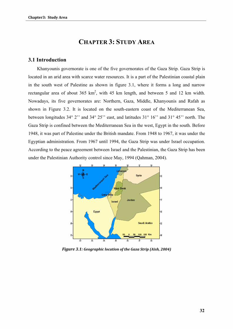
Chapter3: Study Area
32
CHAPTER 3: STUDY AREA
3.1 Introduction Khanyounis governorate is one of the five governorates of the Gaza Strip. Gaza Strip is
located in an arid area with scarce water resources. It is a part of the Palestinian coastal plain
in the south west of Palestine as shown in figure 3.1, where it forms a long and narrow
rectangular area of about 365 km2, with 45 km length, and between 5 and 12 km width.
Nowadays, its five governorates are: Northern, Gaza, Middle, Khanyounis and Rafah as
shown in Figure 3.2. It is located on the south-eastern coast of the Mediterranean Sea,
between longitudes 34° 2’’ and 34° 25’’ east, and latitudes 31° 16’’ and 31° 45’’ north. The
Gaza Strip is confined between the Mediterranean Sea in the west, Egypt in the south. Before
1948, it was part of Palestine under the British mandate. From 1948 to 1967, it was under the
Egyptian administration. From 1967 until 1994, the Gaza Strip was under Israel occupation.
According to the peace agreement between Israel and the Palestinian, the Gaza Strip has been
under the Palestinian Authority control since May, 1994 (Qahman, 2004).
Figure 3.1: Geographic location of the Gaza Strip (Aish, 2004)
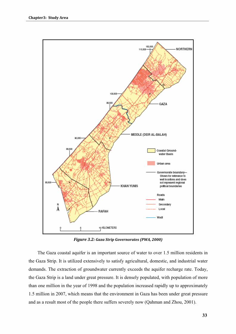
Chapter3: Study Area
33
Figure 3.2: Gaza Strip Governorates (PWA, 2000)
The Gaza coastal aquifer is an important source of water to over 1.5 million residents in
the Gaza Strip. It is utilized extensively to satisfy agricultural, domestic, and industrial water
demands. The extraction of groundwater currently exceeds the aquifer recharge rate. Today,
the Gaza Strip is a land under great pressure. It is densely populated, with population of more
than one million in the year of 1998 and the population increased rapidly up to approximately
1.5 million in 2007, which means that the environment in Gaza has been under great pressure
and as a result most of the people there suffers severely now (Qahman and Zhou, 2001).
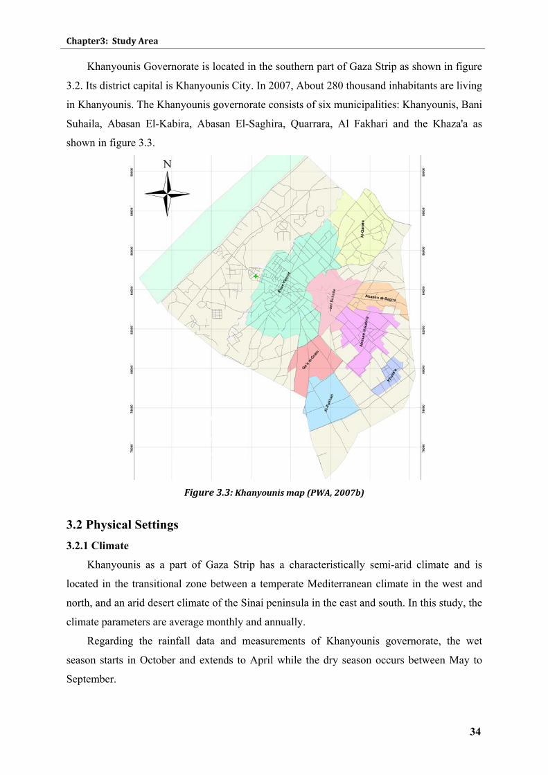
Chapter3: Study Area
34
Khanyounis Governorate is located in the southern part of Gaza Strip as shown in figure
3.2. Its district capital is Khanyounis City. In 2007, About 280 thousand inhabitants are living
in Khanyounis. The Khanyounis governorate consists of six municipalities: Khanyounis, Bani
Suhaila, Abasan El-Kabira, Abasan El-Saghira, Quarrara, Al Fakhari and the Khaza'a as
shown in figure 3.3.
Figure 3.3: Khanyounis map (PWA, 2007b)
3.2 Physical Settings 3.2.1 Climate
Khanyounis as a part of Gaza Strip has a characteristically semi-arid climate and is
located in the transitional zone between a temperate Mediterranean climate in the west and
north, and an arid desert climate of the Sinai peninsula in the east and south. In this study, the
climate parameters are average monthly and annually.
Regarding the rainfall data and measurements of Khanyounis governorate, the wet
season starts in October and extends to April while the dry season occurs between May to
September.
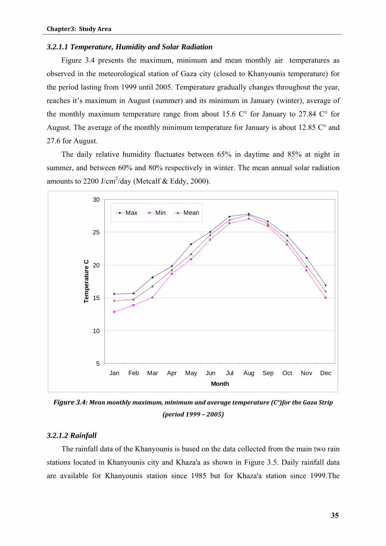
Chapter3: Study Area
35
3.2.1.1 Temperature, Humidity and Solar Radiation
Figure 3.4 presents the maximum, minimum and mean monthly air temperatures as
observed in the meteorological station of Gaza city (closed to Khanyounis temperature) for
the period lasting from 1999 until 2005. Temperature gradually changes throughout the year,
reaches it’s maximum in August (summer) and its minimum in January (winter), average of
the monthly maximum temperature range from about 15.6 C° for January to 27.84 C° for
August. The average of the monthly minimum temperature for January is about 12.85 C° and
27.6 for August.
The daily relative humidity fluctuates between 65% in daytime and 85% at night in
summer, and between 60% and 80% respectively in winter. The mean annual solar radiation
amounts to 2200 J/cm2/day (Metcalf & Eddy, 2000).
5
10
15
20
25
30
Jan Feb Mar Apr May Jun Jul Aug Sep Oct Nov Dec
Month
Tem
pera
ture
C
Max Min Mean
Figure 3.4: Mean monthly maximum, minimum and average temperature (C°)for the Gaza Strip
(period 1999 – 2005)
3.2.1.2 Rainfall
The rainfall data of the Khanyounis is based on the data collected from the main two rain
stations located in Khanyounis city and Khaza'a as shown in Figure 3.5. Daily rainfall data
are available for Khanyounis station since 1985 but for Khaza'a station since 1999.The
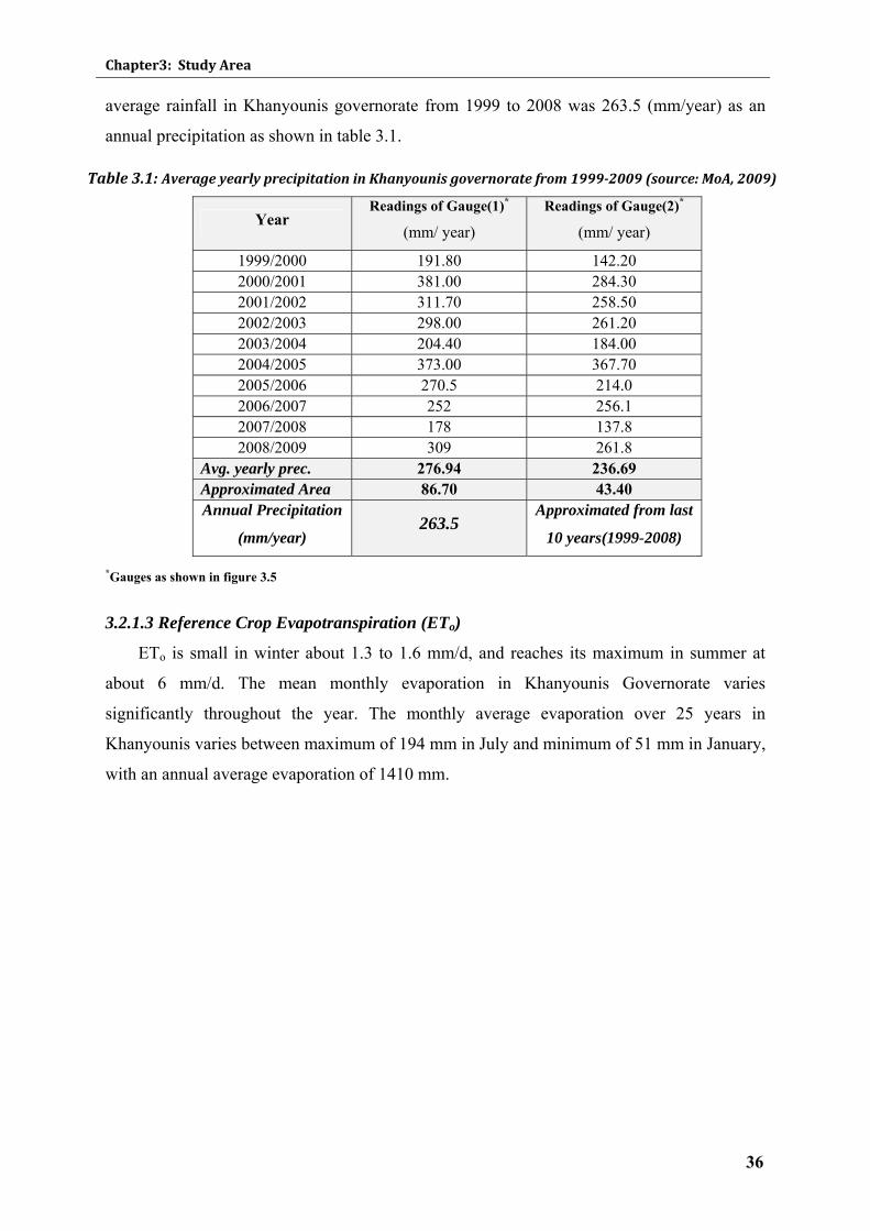
Chapter3: Study Area
36
average rainfall in Khanyounis governorate from 1999 to 2008 was 263.5 (mm/year) as an
annual precipitation as shown in table 3.1.
Table 3.1: Average yearly precipitation in Khanyounis governorate from 19992009 (source: MoA, 2009)
Year Readings of Gauge(1)*
(mm/ year)
Readings of Gauge(2)*
(mm/ year)
1999/2000 191.80 142.20 2000/2001 381.00 284.30 2001/2002 311.70 258.50 2002/2003 298.00 261.20 2003/2004 204.40 184.00 2004/2005 373.00 367.70 2005/2006 270.5 214.0 2006/2007 252 256.1 2007/2008 178 137.8 2008/2009 309 261.8
Avg. yearly prec. 276.94 236.69 Approximated Area 86.70 43.40
Annual Precipitation
(mm/year) 263.5
Approximated from last
10 years(1999-2008)
*Gauges as shown in figure 3.5
3.2.1.3 Reference Crop Evapotranspiration (ETo)
ETo is small in winter about 1.3 to 1.6 mm/d, and reaches its maximum in summer at
about 6 mm/d. The mean monthly evaporation in Khanyounis Governorate varies
significantly throughout the year. The monthly average evaporation over 25 years in
Khanyounis varies between maximum of 194 mm in July and minimum of 51 mm in January,
with an annual average evaporation of 1410 mm.
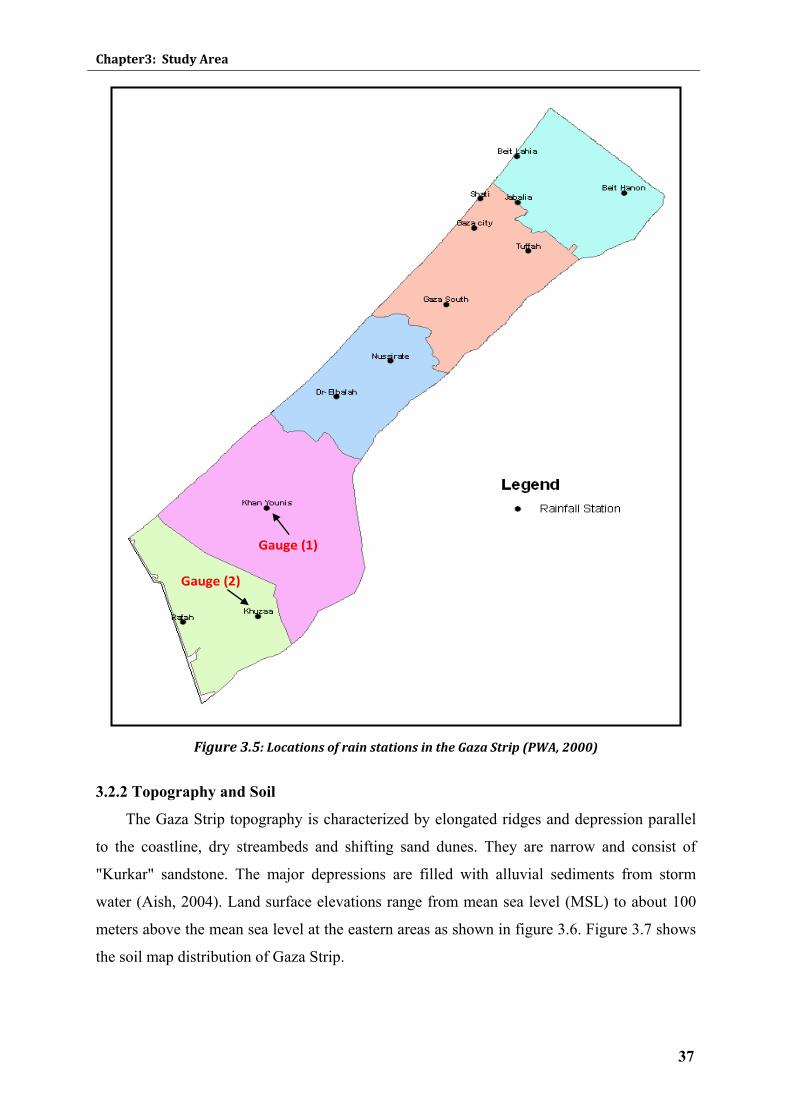
Chapter3: Study Area
37
Figure 3.5: Locations of rain stations in the Gaza Strip (PWA, 2000)
3.2.2 Topography and Soil
The Gaza Strip topography is characterized by elongated ridges and depression parallel
to the coastline, dry streambeds and shifting sand dunes. They are narrow and consist of
"Kurkar" sandstone. The major depressions are filled with alluvial sediments from storm
water (Aish, 2004). Land surface elevations range from mean sea level (MSL) to about 100
meters above the mean sea level at the eastern areas as shown in figure 3.6. Figure 3.7 shows
the soil map distribution of Gaza Strip.
Gauge (1)
Gauge (2)
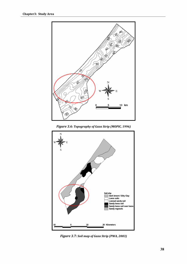
Chapter3: Study Area
38
Figure 3.6: Topography of Gaza Strip (MOPIC, 1996)
Figure 3.7: Soil map of Gaza Strip (PWA, 2003)
10 0 10 20 Kilometers
Soil.shpDark brown / Silty ClayLoess soilsLoessal sandy soilSandy loess soilSandy loess soil over loessSandy regosols
N
EW
S
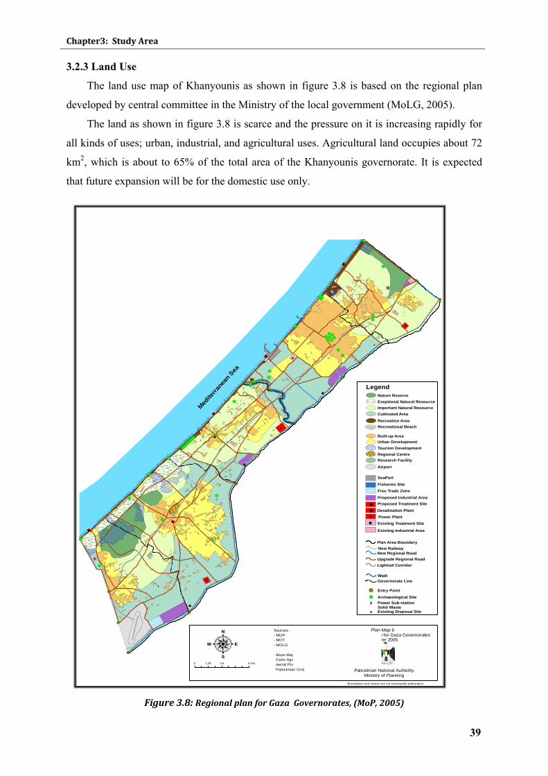
Chapter3: Study Area
39
3.2.3 Land Use
The land use map of Khanyounis as shown in figure 3.8 is based on the regional plan
developed by central committee in the Ministry of the local government (MoLG, 2005).
The land as shown in figure 3.8 is scarce and the pressure on it is increasing rapidly for
all kinds of uses; urban, industrial, and agricultural uses. Agricultural land occupies about 72
km2, which is about to 65% of the total area of the Khanyounis governorate. It is expected
that future expansion will be for the domestic use only.
Figure 3.8: Regional plan for Gaza Governorates, (MoP, 2005)
!.
!.
!.
!.
!.
!.
!.
!.
!.
a
a
!
!
!
!
!
!
"
"
"
"
"
a
"
#
#
#
!(
!(
!(
!(!(
!(
!(
!(
!(
!(
!(
!(
!(!(!(
!(
!(
!(
!(
!(
!(
!(
!(
!(
!(
!(!(!(!(!(!(!(!(
!(!(!(!(!(!(
!(
Medite
rrane
an S
ea
0 2.5 51.25 Km
Legend
Research FacilityRegional Centre
Built-up Area
Recreation Area
Archaeological Site
New RailwayNew Regional RoadUpgrade Regional RoadLightrail Corridor
Airport
Existing Industrial Area
Fisheries SiteFree Trade ZoneProposed Industrial Area
Urban DevelopmentTourism Development
SeaPort
WadiGovernorate Line
!. Entry Point
a Power Sub-stationSolid Waste
# Existing Disposal Site
Plan Area Boundary
Recreational Beach
Nature ReserveExeptional Natural ResourceImportant Natural ResourceCultivated Area
Power Plant
Proposed Treatment SiteDesalination Plant
Existing Treatment Site
!(
:
!
!
"
a
Sources :- MOP- MOT- MOLG
- Base Map Based on Cairo Agreement Map, 1994 Aerial Photos, 1996 Palestinian Grid
Plan Map 6Updated Regional Plan for Gaza Governorates
Palestine 2005
Palestinian National AuthorityMinistry of Planning
Boundaries and names are not necessarily authorative
DRAFT
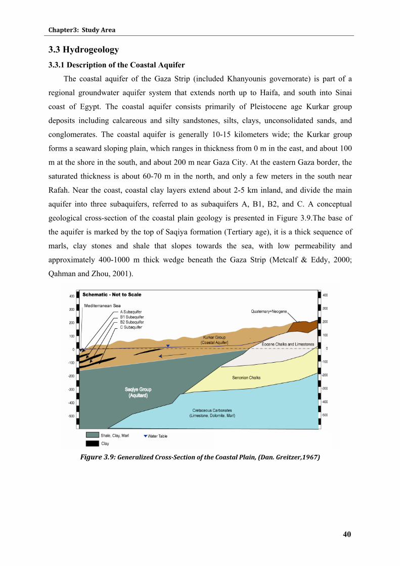
Chapter3: Study Area
40
3.3 Hydrogeology 3.3.1 Description of the Coastal Aquifer
The coastal aquifer of the Gaza Strip (included Khanyounis governorate) is part of a
regional groundwater aquifer system that extends north up to Haifa, and south into Sinai
coast of Egypt. The coastal aquifer consists primarily of Pleistocene age Kurkar group
deposits including calcareous and silty sandstones, silts, clays, unconsolidated sands, and
conglomerates. The coastal aquifer is generally 10-15 kilometers wide; the Kurkar group
forms a seaward sloping plain, which ranges in thickness from 0 m in the east, and about 100
m at the shore in the south, and about 200 m near Gaza City. At the eastern Gaza border, the
saturated thickness is about 60-70 m in the north, and only a few meters in the south near
Rafah. Near the coast, coastal clay layers extend about 2-5 km inland, and divide the main
aquifer into three subaquifers, referred to as subaquifers A, B1, B2, and C. A conceptual
geological cross-section of the coastal plain geology is presented in Figure 3.9.The base of
the aquifer is marked by the top of Saqiya formation (Tertiary age), it is a thick sequence of
marls, clay stones and shale that slopes towards the sea, with low permeability and
approximately 400-1000 m thick wedge beneath the Gaza Strip (Metcalf & Eddy, 2000;
Qahman and Zhou, 2001).
Figure 3.9: Generalized CrossSection of the Coastal Plain, (Dan. Greitzer,1967)
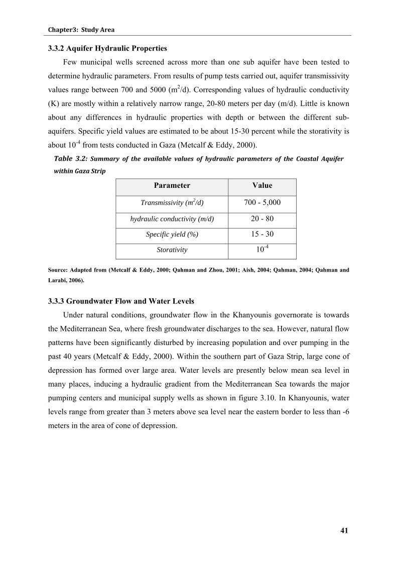
Chapter3: Study Area
41
3.3.2 Aquifer Hydraulic Properties
Few municipal wells screened across more than one sub aquifer have been tested to
determine hydraulic parameters. From results of pump tests carried out, aquifer transmissivity
values range between 700 and 5000 (m2/d). Corresponding values of hydraulic conductivity
(K) are mostly within a relatively narrow range, 20-80 meters per day (m/d). Little is known
about any differences in hydraulic properties with depth or between the different sub-
aquifers. Specific yield values are estimated to be about 15-30 percent while the storativity is
about 10-4 from tests conducted in Gaza (Metcalf & Eddy, 2000).
Table 3.2: Summary of the available values of hydraulic parameters of the Coastal Aquifer
within Gaza Strip
Parameter Value
Transmissivity (m2/d) 700 - 5,000
hydraulic conductivity (m/d) 20 - 80
Specific yield (%) 15 - 30
Storativity 10-4
Source: Adapted from (Metcalf & Eddy, 2000; Qahman and Zhou, 2001; Aish, 2004; Qahman, 2004; Qahman and
Larabi, 2006).
3.3.3 Groundwater Flow and Water Levels
Under natural conditions, groundwater flow in the Khanyounis governorate is towards
the Mediterranean Sea, where fresh groundwater discharges to the sea. However, natural flow
patterns have been significantly disturbed by increasing population and over pumping in the
past 40 years (Metcalf & Eddy, 2000). Within the southern part of Gaza Strip, large cone of
depression has formed over large area. Water levels are presently below mean sea level in
many places, inducing a hydraulic gradient from the Mediterranean Sea towards the major
pumping centers and municipal supply wells as shown in figure 3.10. In Khanyounis, water
levels range from greater than 3 meters above sea level near the eastern border to less than -6
meters in the area of cone of depression.
Chapter3: Study Area
42
Figure 3.10: Water level elevation map for hydrological year 2007 (CMWU,2008).
3.4 Water Quality Ongoing deterioration of the water supply of Gaza Strip poses a major challenge for
water planners and sustainable management of the coastal aquifer. The aquifer is presently
being overexploited, with total pumping exceeding total recharge. In addition, anthropogenic
sources of pollution threaten the water supplies in major urban centers. Many water quality
parameters presently exceed World Health Organization (WHO) drinking water standards.
The major documented water quality problems are elevated chloride (salinity) and nitrate
concentrations in the aquifer (Aish, 2004).
3.4.1 Groundwater Salinity (Chloride)
Salinity in the Gaza coastal aquifer is most often described by the concentration of
chloride in groundwater. Sea water intrusion and intensive exploitation of groundwater have
resulted in increased salinity in the most areas in Gaza Strip. According to CMWU, a
generalized contour map of year 2007 is shown in figure 3.11. Chloride concentrations are
the highest along the Gaza border in the middle and south areas with concentrations
exceeding 1500 mg/l. The best water quality is founded in the sand dune areas in the north,
mainly in the range of 50 – 250 mg/l.
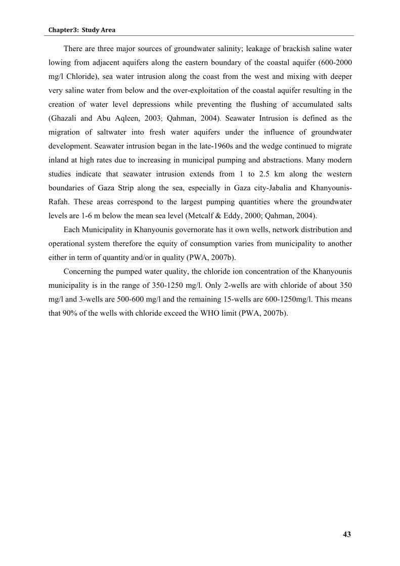
Chapter3: Study Area
43
There are three major sources of groundwater salinity; leakage of brackish saline water
lowing from adjacent aquifers along the eastern boundary of the coastal aquifer (600-2000
mg/l Chloride), sea water intrusion along the coast from the west and mixing with deeper
very saline water from below and the over-exploitation of the coastal aquifer resulting in the
creation of water level depressions while preventing the flushing of accumulated salts
(Ghazali and Abu Aqleen, 2003; Qahman, 2004). Seawater Intrusion is defined as the
migration of saltwater into fresh water aquifers under the influence of groundwater
development. Seawater intrusion began in the late-1960s and the wedge continued to migrate
inland at high rates due to increasing in municipal pumping and abstractions. Many modern
studies indicate that seawater intrusion extends from 1 to 2.5 km along the western
boundaries of Gaza Strip along the sea, especially in Gaza city-Jabalia and Khanyounis-
Rafah. These areas correspond to the largest pumping quantities where the groundwater
levels are 1-6 m below the mean sea level (Metcalf & Eddy, 2000; Qahman, 2004).
Each Municipality in Khanyounis governorate has it own wells, network distribution and
operational system therefore the equity of consumption varies from municipality to another
either in term of quantity and/or in quality (PWA, 2007b).
Concerning the pumped water quality, the chloride ion concentration of the Khanyounis
municipality is in the range of 350-1250 mg/l. Only 2-wells are with chloride of about 350
mg/l and 3-wells are 500-600 mg/l and the remaining 15-wells are 600-1250mg/l. This means
that 90% of the wells with chloride exceed the WHO limit (PWA, 2007b).
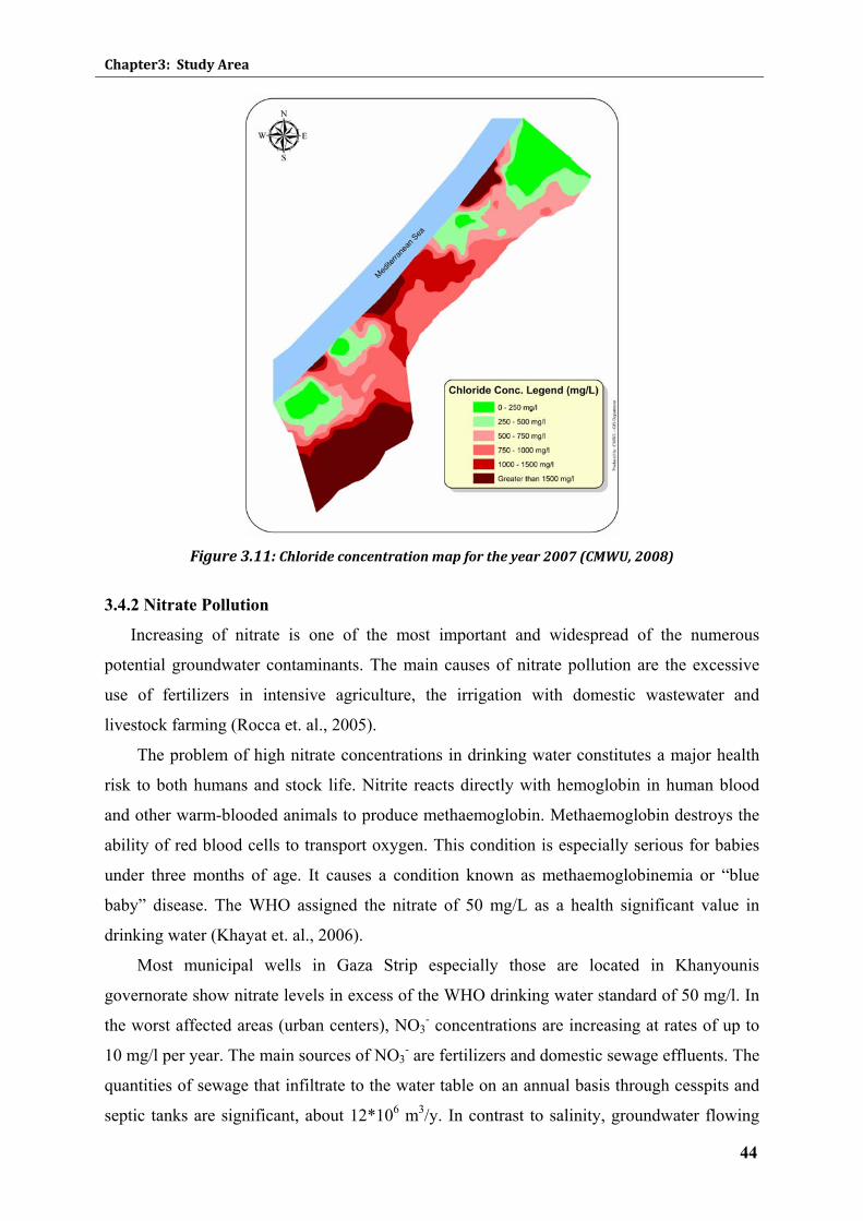
Chapter3: Study Area
44
Figure 3.11: Chloride concentration map for the year 2007 (CMWU, 2008)
3.4.2 Nitrate Pollution
Increasing of nitrate is one of the most important and widespread of the numerous
potential groundwater contaminants. The main causes of nitrate pollution are the excessive
use of fertilizers in intensive agriculture, the irrigation with domestic wastewater and
livestock farming (Rocca et. al., 2005).
The problem of high nitrate concentrations in drinking water constitutes a major health
risk to both humans and stock life. Nitrite reacts directly with hemoglobin in human blood
and other warm-blooded animals to produce methaemoglobin. Methaemoglobin destroys the
ability of red blood cells to transport oxygen. This condition is especially serious for babies
under three months of age. It causes a condition known as methaemoglobinemia or “blue
baby” disease. The WHO assigned the nitrate of 50 mg/L as a health significant value in
drinking water (Khayat et. al., 2006).
Most municipal wells in Gaza Strip especially those are located in Khanyounis
governorate show nitrate levels in excess of the WHO drinking water standard of 50 mg/l. In
the worst affected areas (urban centers), NO3- concentrations are increasing at rates of up to
10 mg/l per year. The main sources of NO3- are fertilizers and domestic sewage effluents. The
quantities of sewage that infiltrate to the water table on an annual basis through cesspits and
septic tanks are significant, about 12*106 m3/y. In contrast to salinity, groundwater flowing
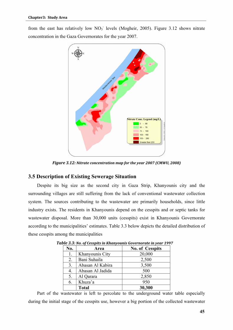
Chapter3: Study Area
45
from the east has relatively low NO3- levels (Mogheir, 2005). Figure 3.12 shows nitrate
concentration in the Gaza Governorates for the year 2007.
Figure 3.12: Nitrate concentration map for the year 2007 (CMWU, 2008)
3.5 Description of Existing Sewerage Situation Despite its big size as the second city in Gaza Strip, Khanyounis city and the
surrounding villages are still suffering from the lack of conventional wastewater collection
system. The sources contributing to the wastewater are primarily households, since little
industry exists. The residents in Khanyounis depend on the cesspits and or septic tanks for
wastewater disposal. More than 30,000 units (cesspits) exist in Khanyounis Governorate
according to the municipalities’ estimates. Table 3.3 below depicts the detailed distribution of
these cesspits among the municipalities
Table 3.3: No. of Cesspits in Khanyounis Governorate in year 1997 No. Area No. of Cesspits 1. Khanyounis City 20,000 2. Bani Suhaila 2,500 3. Abasan Al Kabira 3,500 4. Abasan Al Jadida 500 5. Al Qarara 2,850 6. Khuza’a 950
Total 30,300 Part of the wastewater is left to percolate to the underground water table especially
during the initial stage of the cesspits use, however a big portion of the collected wastewater
Chapter3: Study Area
46
is evacuated by suction trucks and disposed off finally to Wastewater Lagoons located in the
Eastern Area without any treatment. The lagoons are not protected with lining layers. This
contributes to several health and environmental impacts.
Recently, a sewerage collection and pumping system has been implemented that covered
a large area of Khanyounis city. The designed system comprises (80Km) main collection
networks, three main pumping stations and conveyance lines (pressure / gravity). According
to the Finland project in cooperation with PWA the Khanyounis governorate waste water
network is shown in figure 3.13. All components of the network were implemented unless
WWTP and reuse systems which have been suspended as a result of the political conditions
of the Gaza Strip.
Figure 3.13: Scheme for Khanyounis governorate waste water network (PWA, 2007)
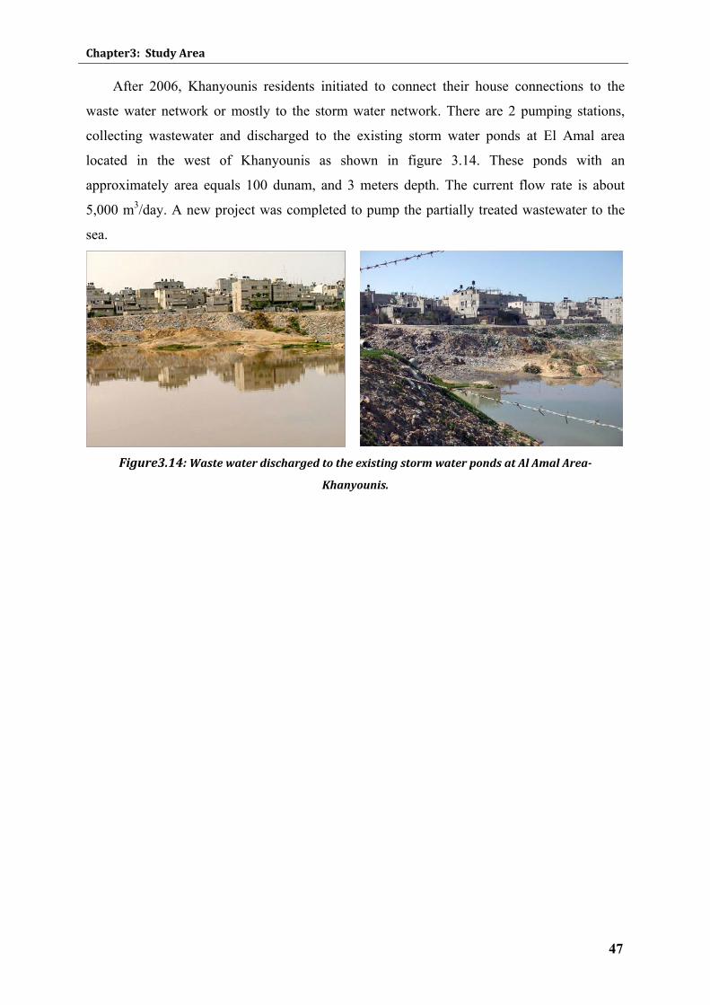
Chapter3: Study Area
47
After 2006, Khanyounis residents initiated to connect their house connections to the
waste water network or mostly to the storm water network. There are 2 pumping stations,
collecting wastewater and discharged to the existing storm water ponds at El Amal area
located in the west of Khanyounis as shown in figure 3.14. These ponds with an
approximately area equals 100 dunam, and 3 meters depth. The current flow rate is about
5,000 m3/day. A new project was completed to pump the partially treated wastewater to the
sea.
Figure3.14: Waste water discharged to the existing storm water ponds at Al Amal Area
Khanyounis.
Chapter4: Groundwater Modeling
48
CHAPTER 4
GROUNDWATER
MODELING
Chapter4: Groundwater Modeling
49
CHAPTER 4: GROUNDWATER MODELING
4.1 Introduction A fully three-dimensional, coupled flow and transport model was used to simulate the
southern part of Gaza coastal aquifer system. Most importantly, the model should ultimately
serve as an aquifer management tool so it can be used to examine and monitor specific
aquifer management actions, and to track the response of the aquifer in conjunction with
aquifer monitoring data.
A conceptual model was first developed to depict the hydrogeology of the aquifer
system, and on its basis, a finite difference model (VMODFLOW Pro.) was applied in three
consecutive steps; (a) the flow model calibration step in which the estimation of hydraulic
conductivity field was conducted and water balances over the aquifer were calculated under
steady state conditions, and storage coefficients and the specific yields were calibrated under
transient conditions, (b) the model transport calibration step in which the estimation of
dispersivity for the movement and fate of nitrate was made, and (c) the simulation step in
which the calibrated flow and transport model was applied to test various management
scenarios of reducing nitrate concentrations in the aquifer system.
In this chapter, the setting up of the flow and transport models will be discussed in
details. The steady and transient states flow calibration steps and results will be discussed in
the next sections in this chapter providing the calibrated parameters. Also, calibration under
transient conditions is reported.
Figure 4.1 is a flow chart of the modeling process in general as applied to the southern
part of Gaza coastal aquifer system.
4.2 Modeling Code and Principles The VMODFLOW Pro. Computer code was applied for simulation of three dimensional
coupled flows and transport of nitrate in Gaza coastal aquifer. It is a numerical engine based
on finite difference grid. The flow processes and the transport process require specific
information about the finite-difference grid such as column widths, row heights, and the top
and bottom of each layer or layer thicknesses.
The full version of VMODFLOW Pro is an integrated package combines MODFLOW,
MODPATH, Zone Budget, MT3D/RT3D, and WinPEST with a powerful available graphical
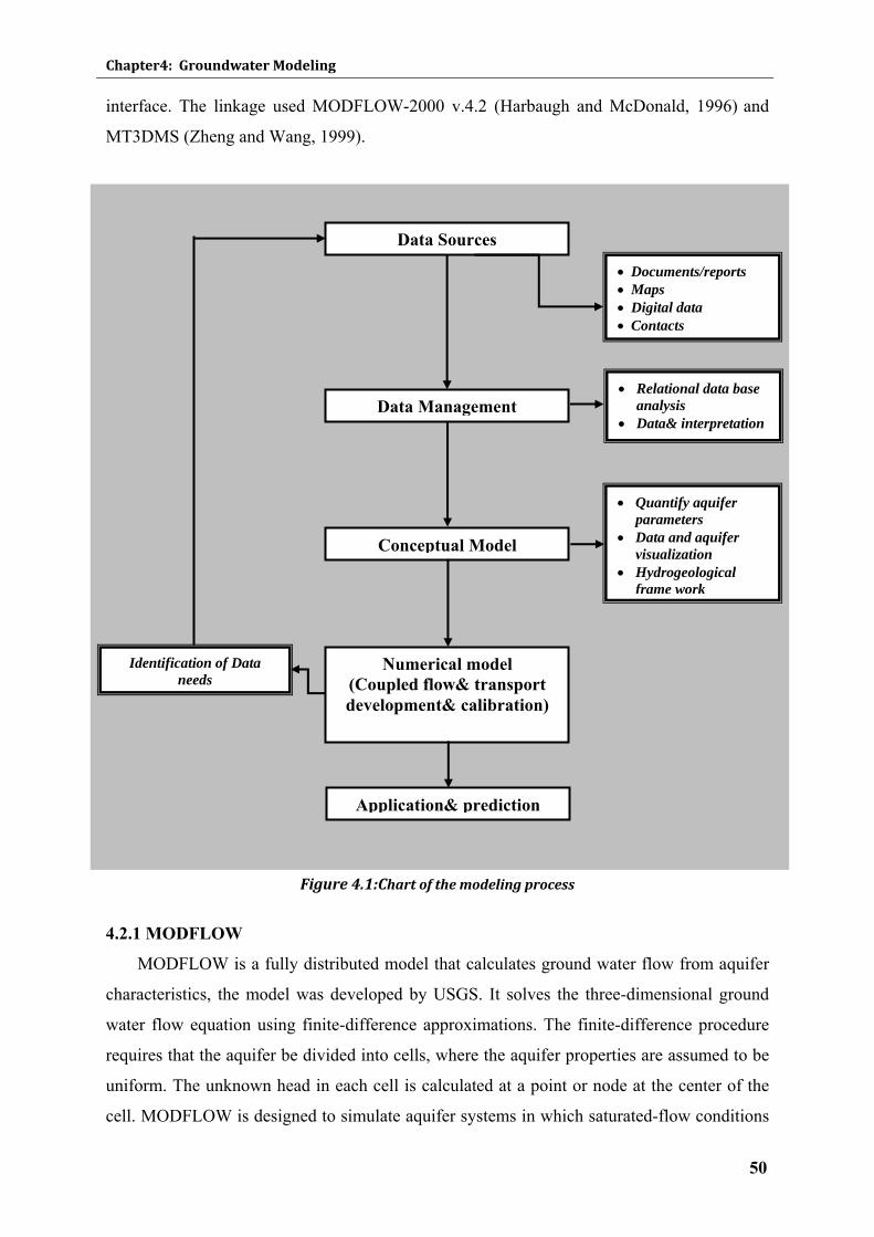
Chapter4: Groundwater Modeling
50
interface. The linkage used MODFLOW-2000 v.4.2 (Harbaugh and McDonald, 1996) and
MT3DMS (Zheng and Wang, 1999).
Figure 4.1:Chart of the modeling process
4.2.1 MODFLOW
MODFLOW is a fully distributed model that calculates ground water flow from aquifer
characteristics, the model was developed by USGS. It solves the three-dimensional ground
water flow equation using finite-difference approximations. The finite-difference procedure
requires that the aquifer be divided into cells, where the aquifer properties are assumed to be
uniform. The unknown head in each cell is calculated at a point or node at the center of the
cell. MODFLOW is designed to simulate aquifer systems in which saturated-flow conditions
Data Sources
Conceptual Model
Numerical model (Coupled flow& transport development& calibration)
Data Management
Application& prediction
• Documents/reports • Maps • Digital data • Contacts
• Relational data base analysis
• Data& interpretation
• Quantify aquifer parameters
• Data and aquifer visualization
• Hydrogeological frame work
Identification of Data needs
Chapter4: Groundwater Modeling
51
exist, Darcy’s Law is applied, the density of ground water is constant, and the principal
directions of horizontal hydraulic conductivity do not vary within the system.
4.2.2 MODPATH
MODPATH is an extension of MODFLOW to calculate flow paths and travel times of
water particles. The model was also developed by USGS. Simulation results obtained with
MODFLOW are used as input to MODPATH. The streamlines and travel times of water
particles can be calculated starting from the groundwater flow velocities using Darcy’s law
(De Smedt, 2003).
4.2.3 MT3DMS
MT3DMS is a three-dimensional groundwater contaminant and solute transport model
that can simulate advection, dispersion, mass transfer, and chemical reactions of dissolved
constituents in ground water. MT3DMS uses the output head and cell-by-cell flow data
computed by MODFLOW to establish the ground water flow field.
4.3 Data Management To develop the flow and transport models, all available data collected for Gaza costal
aquifer -especially southern part of it- should be added to the modeling data base. This
applies to historical and future new data. Specific data items that needed to enter into
modeling data base are:
1. Geological maps and cross sections showing the vertical and horizontal extend and
the boundaries of the aquifer.
2. Topographic maps depicting the ground surface elevations, the bases and the
thickness of the aquifer, and surface water bodies.
3. Water level measurements for the selected years of study.
4. Historical rainfall data from all rainfall gauges.
5. Spatial and temporal distribution of groundwater recharge including rainfall data and
return flow estimates.
6. Collection of wells properties within the model domain of the study area enclosing the
numbers of different types of wells.
7. Collection of water quality data (nitrate data) and land use maps.
8. Available data outside the Gaza Strip, for the area within the model domain,
especially the data related to the groundwater quality.
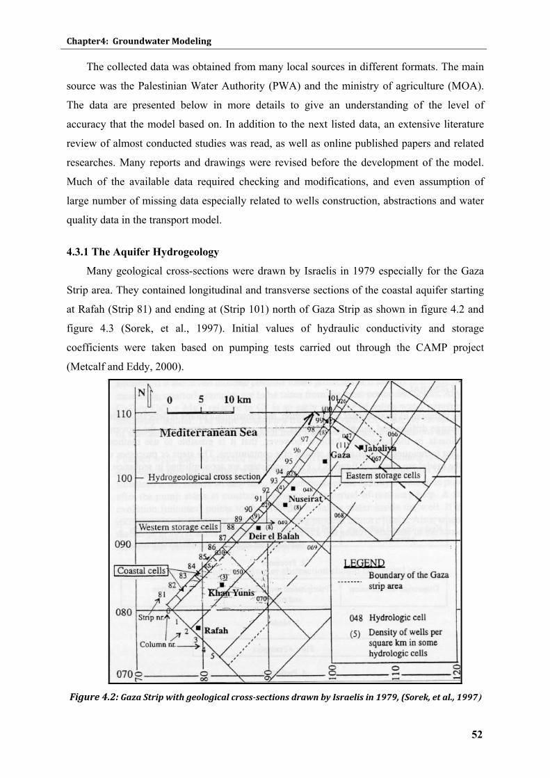
Chapter4: Groundwater Modeling
52
The collected data was obtained from many local sources in different formats. The main
source was the Palestinian Water Authority (PWA) and the ministry of agriculture (MOA).
The data are presented below in more details to give an understanding of the level of
accuracy that the model based on. In addition to the next listed data, an extensive literature
review of almost conducted studies was read, as well as online published papers and related
researches. Many reports and drawings were revised before the development of the model.
Much of the available data required checking and modifications, and even assumption of
large number of missing data especially related to wells construction, abstractions and water
quality data in the transport model.
4.3.1 The Aquifer Hydrogeology
Many geological cross-sections were drawn by Israelis in 1979 especially for the Gaza
Strip area. They contained longitudinal and transverse sections of the coastal aquifer starting
at Rafah (Strip 81) and ending at (Strip 101) north of Gaza Strip as shown in figure 4.2 and
figure 4.3 (Sorek, et al., 1997). Initial values of hydraulic conductivity and storage
coefficients were taken based on pumping tests carried out through the CAMP project
(Metcalf and Eddy, 2000).
Figure 4.2: Gaza Strip with geological crosssections drawn by Israelis in 1979, (Sorek, et al., 1997)
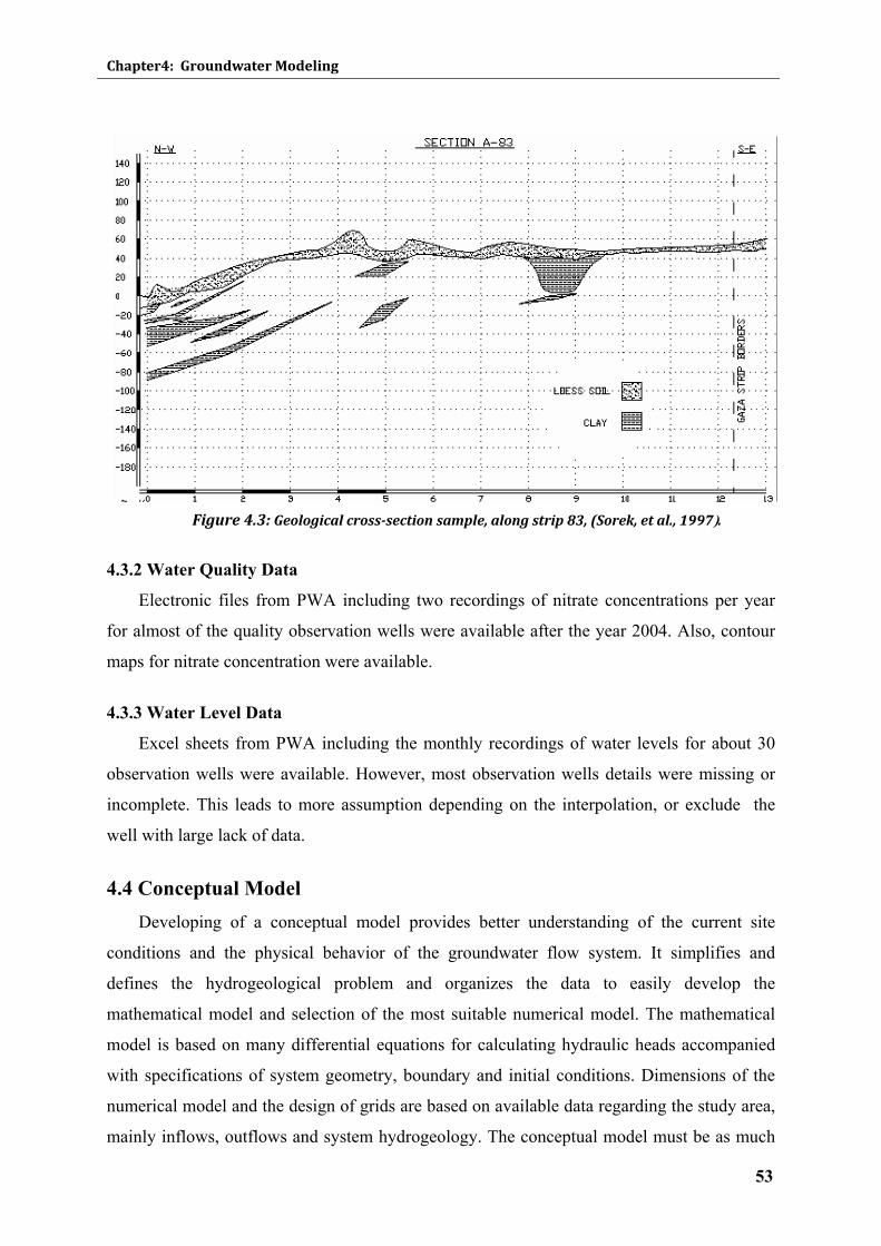
Chapter4: Groundwater Modeling
53
Figure 4.3: Geological crosssection sample, along strip 83, (Sorek, et al., 1997).
4.3.2 Water Quality Data
Electronic files from PWA including two recordings of nitrate concentrations per year
for almost of the quality observation wells were available after the year 2004. Also, contour
maps for nitrate concentration were available.
4.3.3 Water Level Data
Excel sheets from PWA including the monthly recordings of water levels for about 30
observation wells were available. However, most observation wells details were missing or
incomplete. This leads to more assumption depending on the interpolation, or exclude the
well with large lack of data.
4.4 Conceptual Model Developing of a conceptual model provides better understanding of the current site
conditions and the physical behavior of the groundwater flow system. It simplifies and
defines the hydrogeological problem and organizes the data to easily develop the
mathematical model and selection of the most suitable numerical model. The mathematical
model is based on many differential equations for calculating hydraulic heads accompanied
with specifications of system geometry, boundary and initial conditions. Dimensions of the
numerical model and the design of grids are based on available data regarding the study area,
mainly inflows, outflows and system hydrogeology. The conceptual model must be as much
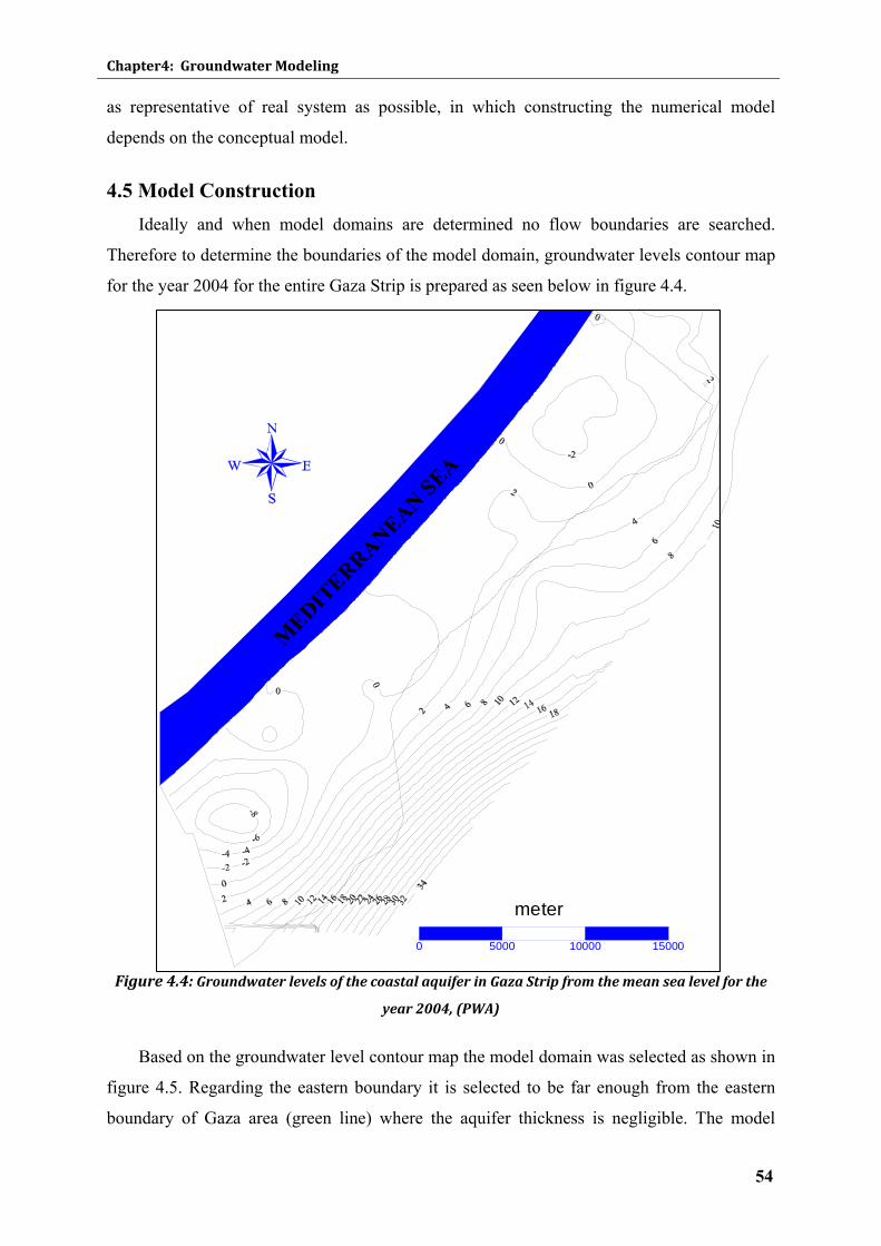
Chapter4: Groundwater Modeling
54
0 5000 10000 15000
meter
Average Groundwater levels in Gaza Strip for the Year 2004
(m-amsl)
MEDIT
ERRANEAN SEA
as representative of real system as possible, in which constructing the numerical model
depends on the conceptual model.
4.5 Model Construction Ideally and when model domains are determined no flow boundaries are searched.
Therefore to determine the boundaries of the model domain, groundwater levels contour map
for the year 2004 for the entire Gaza Strip is prepared as seen below in figure 4.4.
Figure 4.4: Groundwater levels of the coastal aquifer in Gaza Strip from the mean sea level for the
year 2004, (PWA)
Based on the groundwater level contour map the model domain was selected as shown in
figure 4.5. Regarding the eastern boundary it is selected to be far enough from the eastern
boundary of Gaza area (green line) where the aquifer thickness is negligible. The model
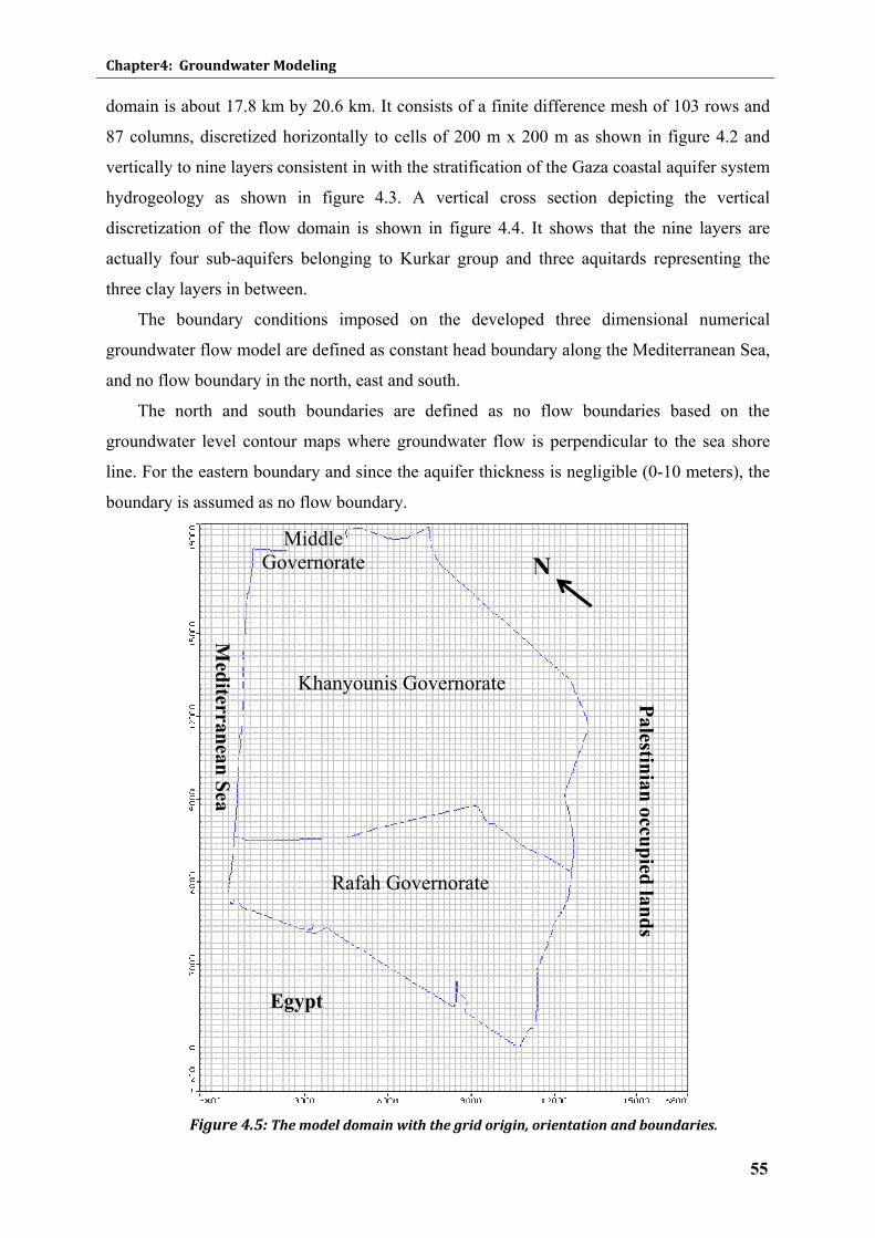
Chapter4: Groundwater Modeling
55
domain is about 17.8 km by 20.6 km. It consists of a finite difference mesh of 103 rows and
87 columns, discretized horizontally to cells of 200 m x 200 m as shown in figure 4.2 and
vertically to nine layers consistent in with the stratification of the Gaza coastal aquifer system
hydrogeology as shown in figure 4.3. A vertical cross section depicting the vertical
discretization of the flow domain is shown in figure 4.4. It shows that the nine layers are
actually four sub-aquifers belonging to Kurkar group and three aquitards representing the
three clay layers in between.
The boundary conditions imposed on the developed three dimensional numerical
groundwater flow model are defined as constant head boundary along the Mediterranean Sea,
and no flow boundary in the north, east and south.
The north and south boundaries are defined as no flow boundaries based on the
groundwater level contour maps where groundwater flow is perpendicular to the sea shore
line. For the eastern boundary and since the aquifer thickness is negligible (0-10 meters), the
boundary is assumed as no flow boundary.
Figure 4.5: The model domain with the grid origin, orientation and boundaries.
Middle Governorate
Khanyounis Governorate
Rafah Governorate
Egypt
Palestinian occupied lands
Mediterranean Sea
N
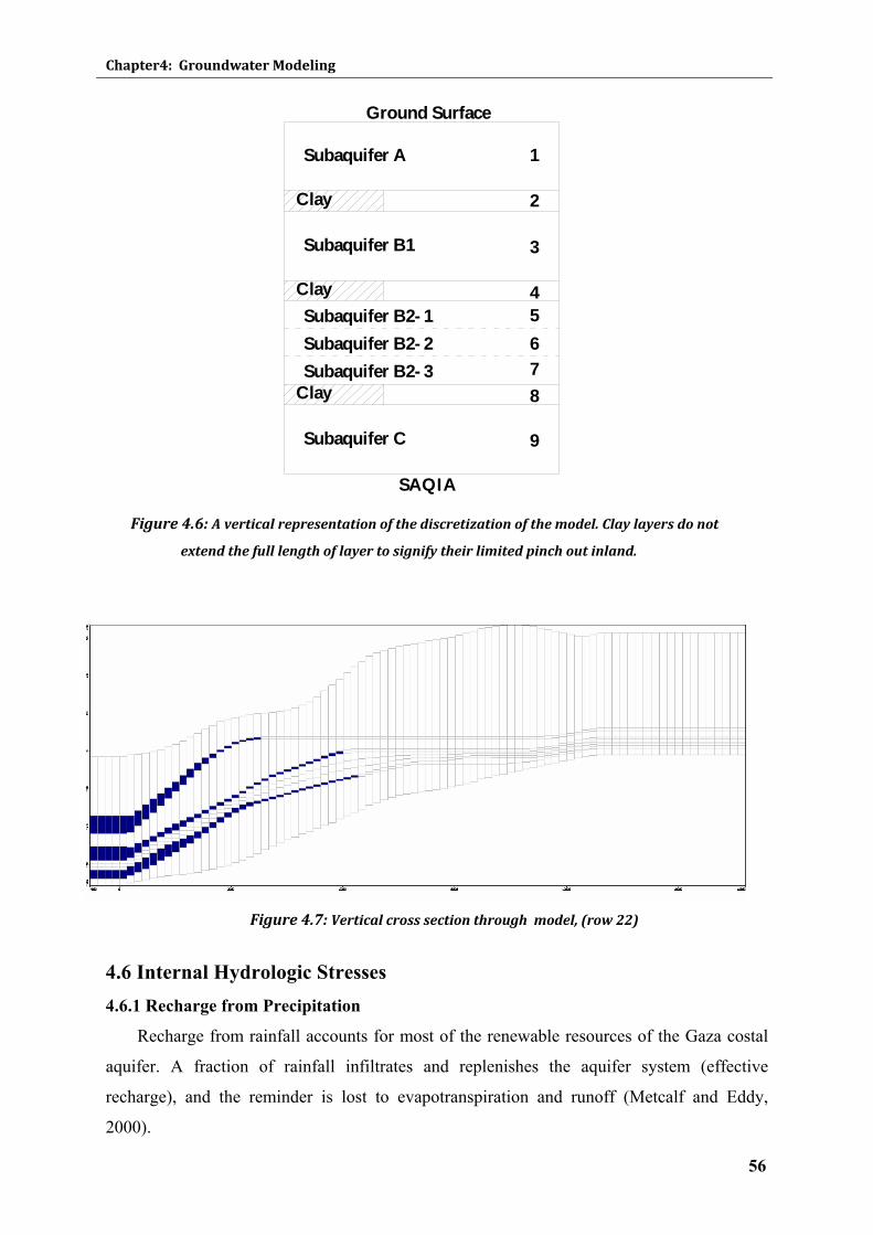
Chapter4: Groundwater Modeling
56
Subaquifer A
Clay
Clay
Clay
Subaquifer B1
Subaquifer C
Subaquifer B2-1Subaquifer B2-2Subaquifer B2-3
SAQIA
1
2
3
45678
9
Ground Surface
Figure 4.6: A vertical representation of the discretization of the model. Clay layers do not
extend the full length of layer to signify their limited pinch out inland.
Figure 4.7: Vertical cross section through model, (row 22)
4.6 Internal Hydrologic Stresses 4.6.1 Recharge from Precipitation
Recharge from rainfall accounts for most of the renewable resources of the Gaza costal
aquifer. A fraction of rainfall infiltrates and replenishes the aquifer system (effective
recharge), and the reminder is lost to evapotranspiration and runoff (Metcalf and Eddy,
2000).
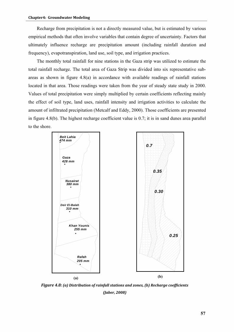
Chapter4: Groundwater Modeling
57
Recharge from precipitation is not a directly measured value, but is estimated by various
empirical methods that often involve variables that contain degree of uncertainty. Factors that
ultimately influence recharge are precipitation amount (including rainfall duration and
frequency), evapotranspiration, land use, soil type, and irrigation practices.
The monthly total rainfall for nine stations in the Gaza strip was utilized to estimate the
total rainfall recharge. The total area of Gaza Strip was divided into six representative sub-
areas as shown in figure 4.8(a) in accordance with available readings of rainfall stations
located in that area. Those readings were taken from the year of steady state study in 2000.
Values of total precipitation were simply multiplied by certain coefficients reflecting mainly
the effect of soil type, land uses, rainfall intensity and irrigation activities to calculate the
amount of infiltrated precipitation (Metcalf and Eddy, 2000). Those coefficients are presented
in figure 4.8(b). The highest recharge coefficient value is 0.7; it is in sand dunes area parallel
to the shore.
Rafah205 mm
Beit Lahia
Gaza
Nusairat380 mm
Deir El-Balah310 mm
Khan Younis255 mm
428 mm
474 mm
(a)
0.25
0.7
0.35
0.30
(b)
Figure 4.8: (a) Distribution of rainfall stations and zones, (b) Recharge coefficients
(Jaber, 2008)
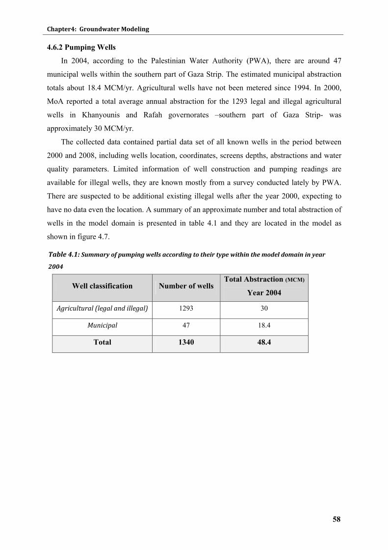
Chapter4: Groundwater Modeling
58
4.6.2 Pumping Wells
In 2004, according to the Palestinian Water Authority (PWA), there are around 47
municipal wells within the southern part of Gaza Strip. The estimated municipal abstraction
totals about 18.4 MCM/yr. Agricultural wells have not been metered since 1994. In 2000,
MoA reported a total average annual abstraction for the 1293 legal and illegal agricultural
wells in Khanyounis and Rafah governorates –southern part of Gaza Strip- was
approximately 30 MCM/yr.
The collected data contained partial data set of all known wells in the period between
2000 and 2008, including wells location, coordinates, screens depths, abstractions and water
quality parameters. Limited information of well construction and pumping readings are
available for illegal wells, they are known mostly from a survey conducted lately by PWA.
There are suspected to be additional existing illegal wells after the year 2000, expecting to
have no data even the location. A summary of an approximate number and total abstraction of
wells in the model domain is presented in table 4.1 and they are located in the model as
shown in figure 4.7.
Table 4.1: Summary of pumping wells according to their type within the model domain in year
2004
Well classification Number of wells
Total Abstraction (MCM)
Year 2004
Agricultural (legal and illegal) 1293 30
Municipal 47 18.4
Total 1340 48.4
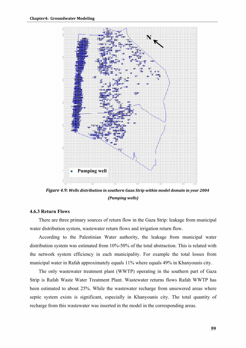
Chapter4: Groundwater Modeling
59
Figure 4.9: Wells distribution in southern Gaza Strip within model domain in year 2004
(Pumping wells)
4.6.3 Return Flows
There are three primary sources of return flow in the Gaza Strip: leakage from municipal
water distribution system, wastewater return flows and irrigation return flow.
According to the Palestinian Water authority, the leakage from municipal water
distribution system was estimated from 10%-50% of the total abstraction. This is related with
the network system efficiency in each municipality. For example the total losses from
municipal water in Rafah approximately equals 11% where equals 49% in Khanyounis city.
The only wastewater treatment plant (WWTP) operating in the southern part of Gaza
Strip is Rafah Waste Water Treatment Plant. Wastewater returns flows Rafah WWTP has
been estimated to about 25%. While the wastewater recharge from unsewered areas where
septic system exists is significant, especially in Khanyounis city. The total quantity of
recharge from this wastewater was inserted in the model in the corresponding areas.
N
Pumping well
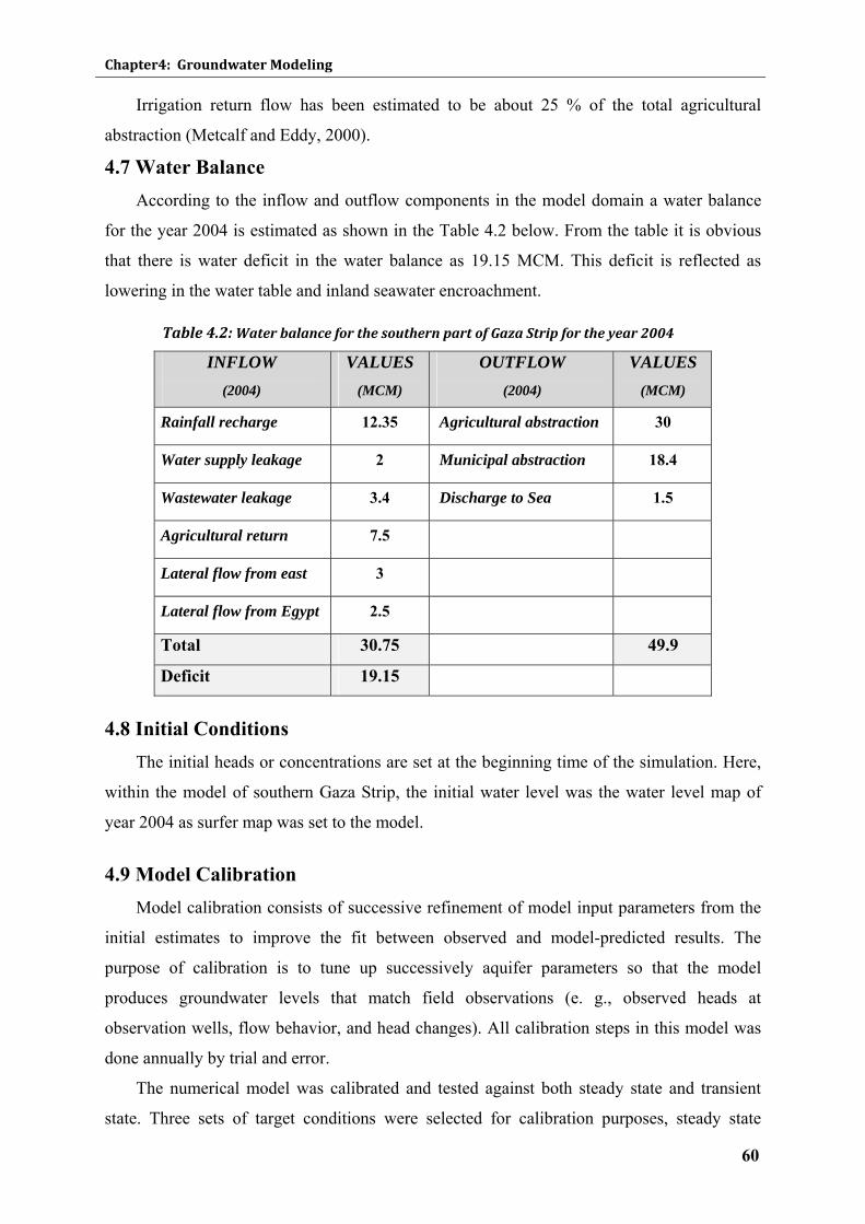
Chapter4: Groundwater Modeling
60
Irrigation return flow has been estimated to be about 25 % of the total agricultural
abstraction (Metcalf and Eddy, 2000).
4.7 Water Balance According to the inflow and outflow components in the model domain a water balance
for the year 2004 is estimated as shown in the Table 4.2 below. From the table it is obvious
that there is water deficit in the water balance as 19.15 MCM. This deficit is reflected as
lowering in the water table and inland seawater encroachment.
Table 4.2: Water balance for the southern part of Gaza Strip for the year 2004
INFLOW (2004)
VALUES (MCM)
OUTFLOW (2004)
VALUES (MCM)
Rainfall recharge 12.35 Agricultural abstraction 30
Water supply leakage 2 Municipal abstraction 18.4
Wastewater leakage 3.4 Discharge to Sea 1.5
Agricultural return 7.5
Lateral flow from east 3
Lateral flow from Egypt 2.5
Total 30.75 49.9
Deficit 19.15
4.8 Initial Conditions The initial heads or concentrations are set at the beginning time of the simulation. Here,
within the model of southern Gaza Strip, the initial water level was the water level map of
year 2004 as surfer map was set to the model.
4.9 Model Calibration Model calibration consists of successive refinement of model input parameters from the
initial estimates to improve the fit between observed and model-predicted results. The
purpose of calibration is to tune up successively aquifer parameters so that the model
produces groundwater levels that match field observations (e. g., observed heads at
observation wells, flow behavior, and head changes). All calibration steps in this model was
done annually by trial and error.
The numerical model was calibrated and tested against both steady state and transient
state. Three sets of target conditions were selected for calibration purposes, steady state
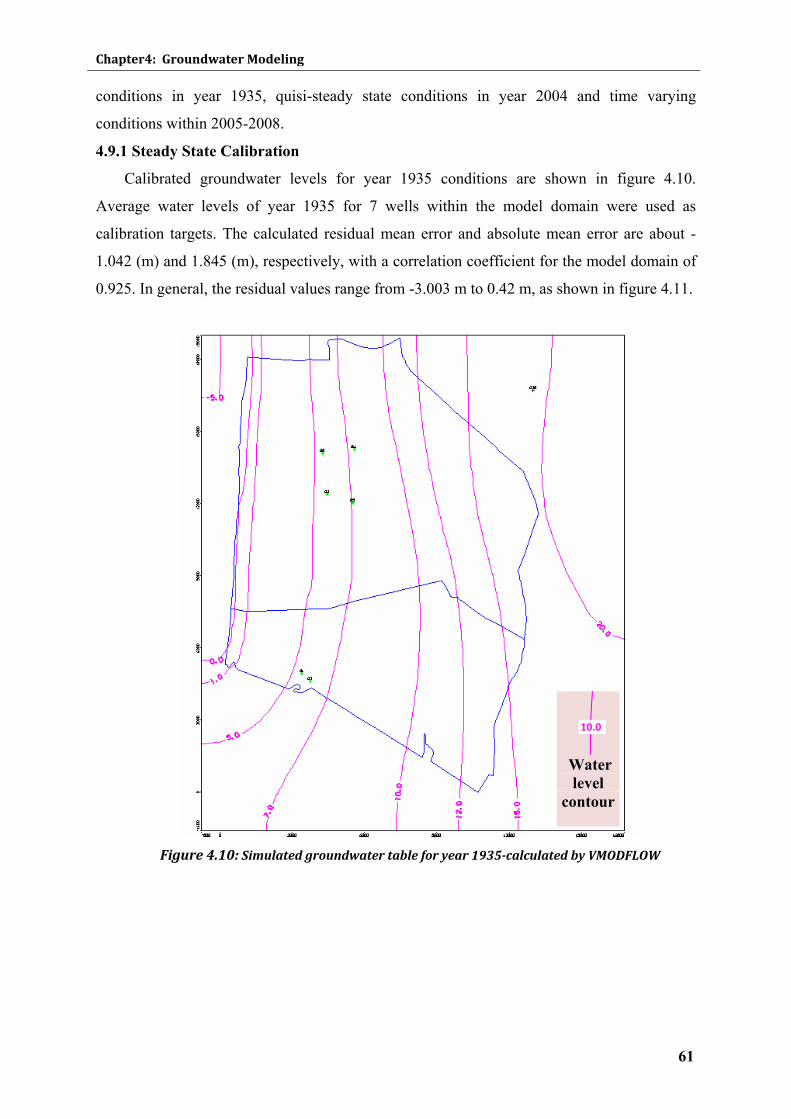
Chapter4: Groundwater Modeling
61
conditions in year 1935, quisi-steady state conditions in year 2004 and time varying
conditions within 2005-2008.
4.9.1 Steady State Calibration
Calibrated groundwater levels for year 1935 conditions are shown in figure 4.10.
Average water levels of year 1935 for 7 wells within the model domain were used as
calibration targets. The calculated residual mean error and absolute mean error are about -
1.042 (m) and 1.845 (m), respectively, with a correlation coefficient for the model domain of
0.925. In general, the residual values range from -3.003 m to 0.42 m, as shown in figure 4.11.
Figure 4.10: Simulated groundwater table for year 1935calculated by VMODFLOW
10.0
Water
level contour
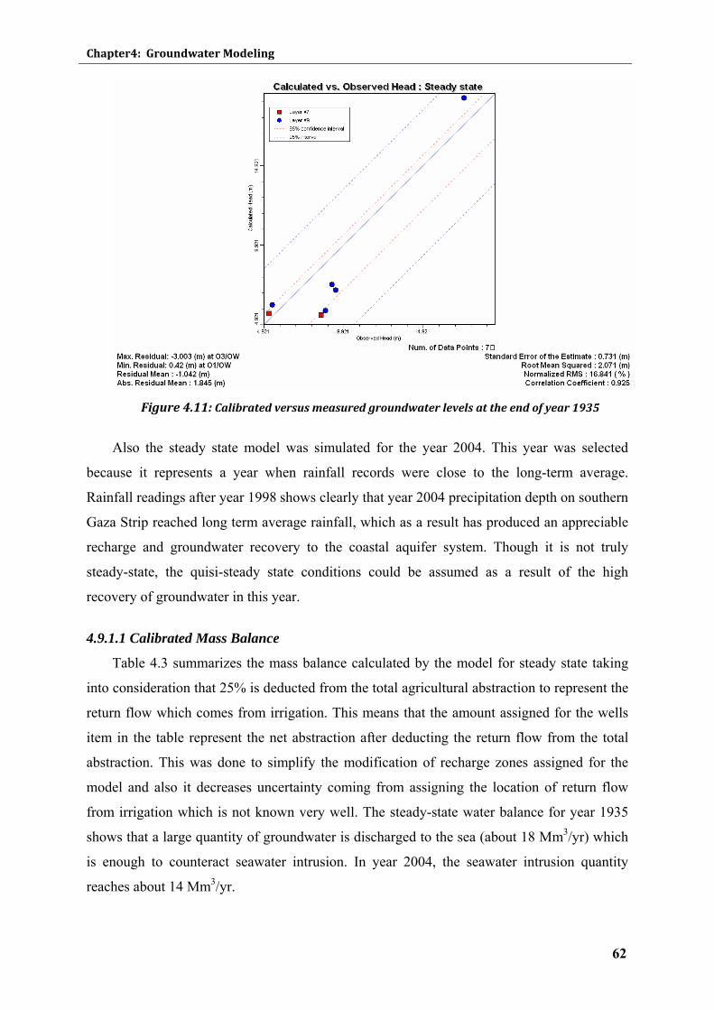
Chapter4: Groundwater Modeling
62
Figure 4.11: Calibrated versus measured groundwater levels at the end of year 1935
Also the steady state model was simulated for the year 2004. This year was selected
because it represents a year when rainfall records were close to the long-term average.
Rainfall readings after year 1998 shows clearly that year 2004 precipitation depth on southern
Gaza Strip reached long term average rainfall, which as a result has produced an appreciable
recharge and groundwater recovery to the coastal aquifer system. Though it is not truly
steady-state, the quisi-steady state conditions could be assumed as a result of the high
recovery of groundwater in this year.
4.9.1.1 Calibrated Mass Balance
Table 4.3 summarizes the mass balance calculated by the model for steady state taking
into consideration that 25% is deducted from the total agricultural abstraction to represent the
return flow which comes from irrigation. This means that the amount assigned for the wells
item in the table represent the net abstraction after deducting the return flow from the total
abstraction. This was done to simplify the modification of recharge zones assigned for the
model and also it decreases uncertainty coming from assigning the location of return flow
from irrigation which is not known very well. The steady-state water balance for year 1935
shows that a large quantity of groundwater is discharged to the sea (about 18 Mm3/yr) which
is enough to counteract seawater intrusion. In year 2004, the seawater intrusion quantity
reaches about 14 Mm3/yr.
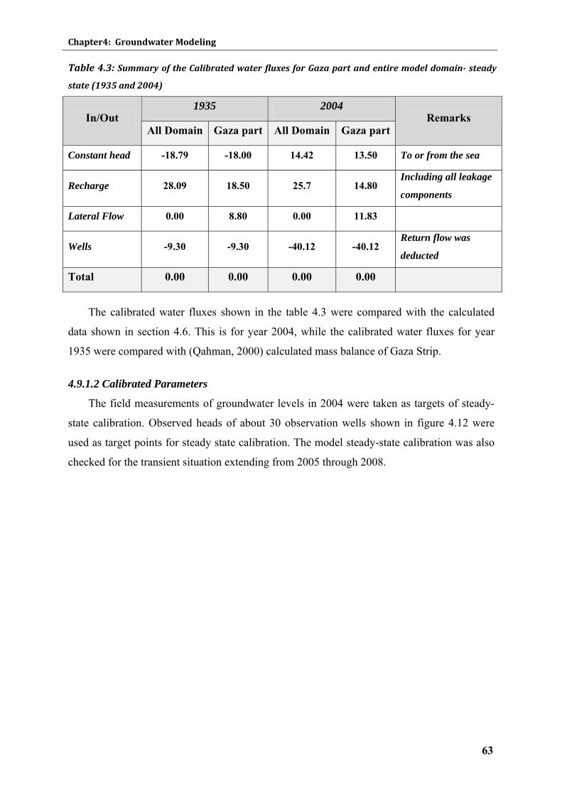
Chapter4: Groundwater Modeling
63
Table 4.3: Summary of the Calibrated water fluxes for Gaza part and entire model domain steady
state (1935 and 2004)
1935 2004 In/Out
All Domain Gaza part All Domain Gaza partRemarks
Constant head -18.79 -18.00 14.42 13.50 To or from the sea
Recharge 28.09 18.50 25.7 14.80 Including all leakage
components
Lateral Flow 0.00 8.80 0.00 11.83
Wells -9.30 -9.30 -40.12 -40.12 Return flow was
deducted
Total 0.00 0.00 0.00 0.00
The calibrated water fluxes shown in the table 4.3 were compared with the calculated
data shown in section 4.6. This is for year 2004, while the calibrated water fluxes for year
1935 were compared with (Qahman, 2000) calculated mass balance of Gaza Strip.
4.9.1.2 Calibrated Parameters
The field measurements of groundwater levels in 2004 were taken as targets of steady-
state calibration. Observed heads of about 30 observation wells shown in figure 4.12 were
used as target points for steady state calibration. The model steady-state calibration was also
checked for the transient situation extending from 2005 through 2008.
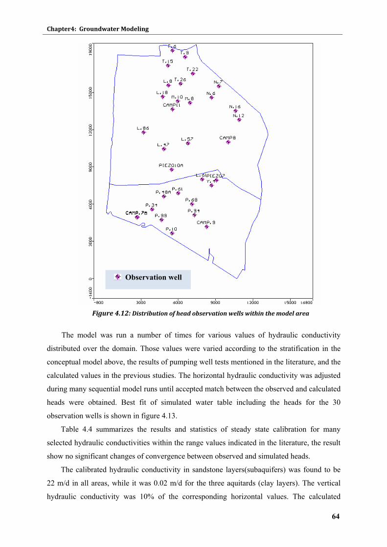
Chapter4: Groundwater Modeling
64
Figure 4.12: Distribution of head observation wells within the model area
The model was run a number of times for various values of hydraulic conductivity
distributed over the domain. Those values were varied according to the stratification in the
conceptual model above, the results of pumping well tests mentioned in the literature, and the
calculated values in the previous studies. The horizontal hydraulic conductivity was adjusted
during many sequential model runs until accepted match between the observed and calculated
heads were obtained. Best fit of simulated water table including the heads for the 30
observation wells is shown in figure 4.13.
Table 4.4 summarizes the results and statistics of steady state calibration for many
selected hydraulic conductivities within the range values indicated in the literature, the result
show no significant changes of convergence between observed and simulated heads.
The calibrated hydraulic conductivity in sandstone layers(subaquifers) was found to be
22 m/d in all areas, while it was 0.02 m/d for the three aquitards (clay layers). The vertical
hydraulic conductivity was 10% of the corresponding horizontal values. The calculated
Observation well
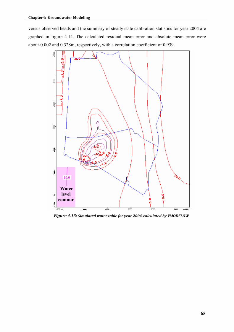
Chapter4: Groundwater Modeling
65
versus observed heads and the summary of steady state calibration statistics for year 2004 are
graphed in figure 4.14. The calculated residual mean error and absolute mean error were
about-0.002 and 0.328m, respectively, with a correlation coefficient of 0.939.
Figure 4.13: Simulated water table for year 2004calculated by VMODFLOW
10.0
Water
level contour
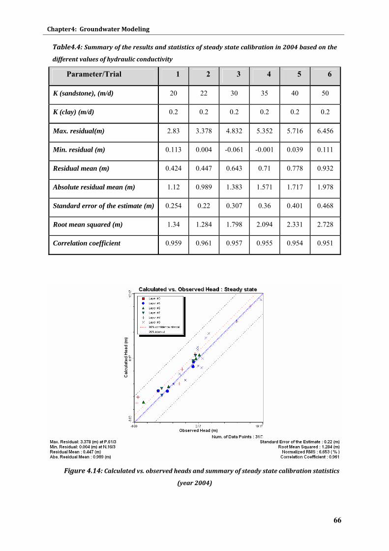
Chapter4: Groundwater Modeling
66
Table4.4: Summary of the results and statistics of steady state calibration in 2004 based on the
different values of hydraulic conductivity
Parameter/Trial 1 2 3 4 5 6
K (sandstone), (m/d) 20 22 30 35 40 50
K (clay) (m/d) 0.2 0.2 0.2 0.2 0.2 0.2
Max. residual(m) 2.83 3.378 4.832 5.352 5.716 6.456
Min. residual (m) 0.113 0.004 -0.061 -0.001 0.039 0.111
Residual mean (m) 0.424 0.447 0.643 0.71 0.778 0.932
Absolute residual mean (m) 1.12 0.989 1.383 1.571 1.717 1.978
Standard error of the estimate (m) 0.254 0.22 0.307 0.36 0.401 0.468
Root mean squared (m) 1.34 1.284 1.798 2.094 2.331 2.728
Correlation coefficient 0.959 0.961 0.957 0.955 0.954 0.951
Figure 4.14: Calculated vs. observed heads and summary of steady state calibration statistics
(year 2004)
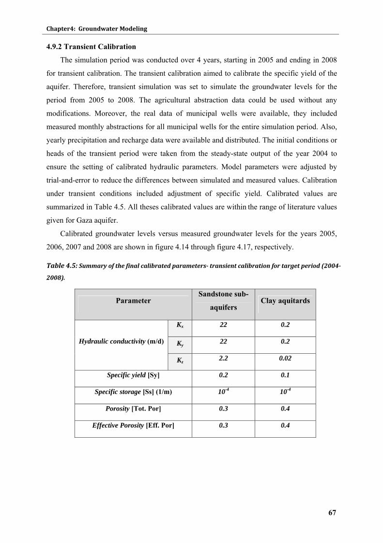
Chapter4: Groundwater Modeling
67
4.9.2 Transient Calibration
The simulation period was conducted over 4 years, starting in 2005 and ending in 2008
for transient calibration. The transient calibration aimed to calibrate the specific yield of the
aquifer. Therefore, transient simulation was set to simulate the groundwater levels for the
period from 2005 to 2008. The agricultural abstraction data could be used without any
modifications. Moreover, the real data of municipal wells were available, they included
measured monthly abstractions for all municipal wells for the entire simulation period. Also,
yearly precipitation and recharge data were available and distributed. The initial conditions or
heads of the transient period were taken from the steady-state output of the year 2004 to
ensure the setting of calibrated hydraulic parameters. Model parameters were adjusted by
trial-and-error to reduce the differences between simulated and measured values. Calibration
under transient conditions included adjustment of specific yield. Calibrated values are
summarized in Table 4.5. All theses calibrated values are within the range of literature values
given for Gaza aquifer.
Calibrated groundwater levels versus measured groundwater levels for the years 2005,
2006, 2007 and 2008 are shown in figure 4.14 through figure 4.17, respectively.
Table 4.5: Summary of the final calibrated parameters transient calibration for target period (2004
2008).
Parameter
Sandstone sub-
aquifers Clay aquitards
Kx 22 0.2
Ky 22 0.2
Hydraulic conductivity (m/d)
Kz 2.2 0.02
Specific yield [Sy] 0.2 0.1
Specific storage [Ss] (1/m) 10-4 10-4
Porosity [Tot. Por] 0.3 0.4
Effective Porosity [Eff. Por] 0.3 0.4
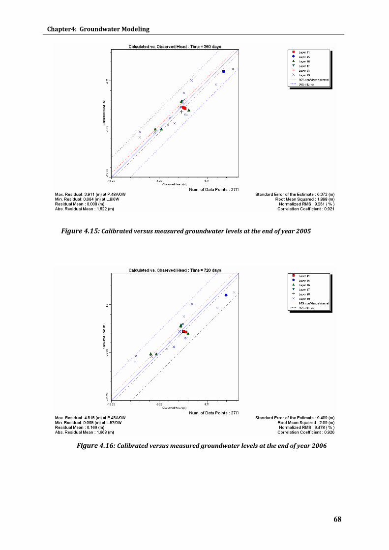
Chapter4: Groundwater Modeling
68
Figure 4.15: Calibrated versus measured groundwater levels at the end of year 2005
Figure 4.16: Calibrated versus measured groundwater levels at the end of year 2006
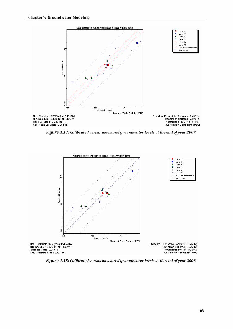
Chapter4: Groundwater Modeling
69
Figure 4.17: Calibrated versus measured groundwater levels at the end of year 2007
Figure 4.18: Calibrated versus measured groundwater levels at the end of year 2008
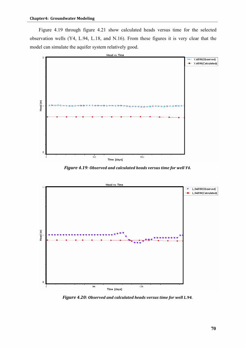
Chapter4: Groundwater Modeling
70
Figure 4.19 through figure 4.21 show calculated heads versus time for the selected
observation wells (Y4, L.94, L.18, and N.16). From these figures it is very clear that the
model can simulate the aquifer system relatively good.
Figure 4.19: Observed and calculated heads versus time for well Y4.
Figure 4.20: Observed and calculated heads versus time for well L.94.
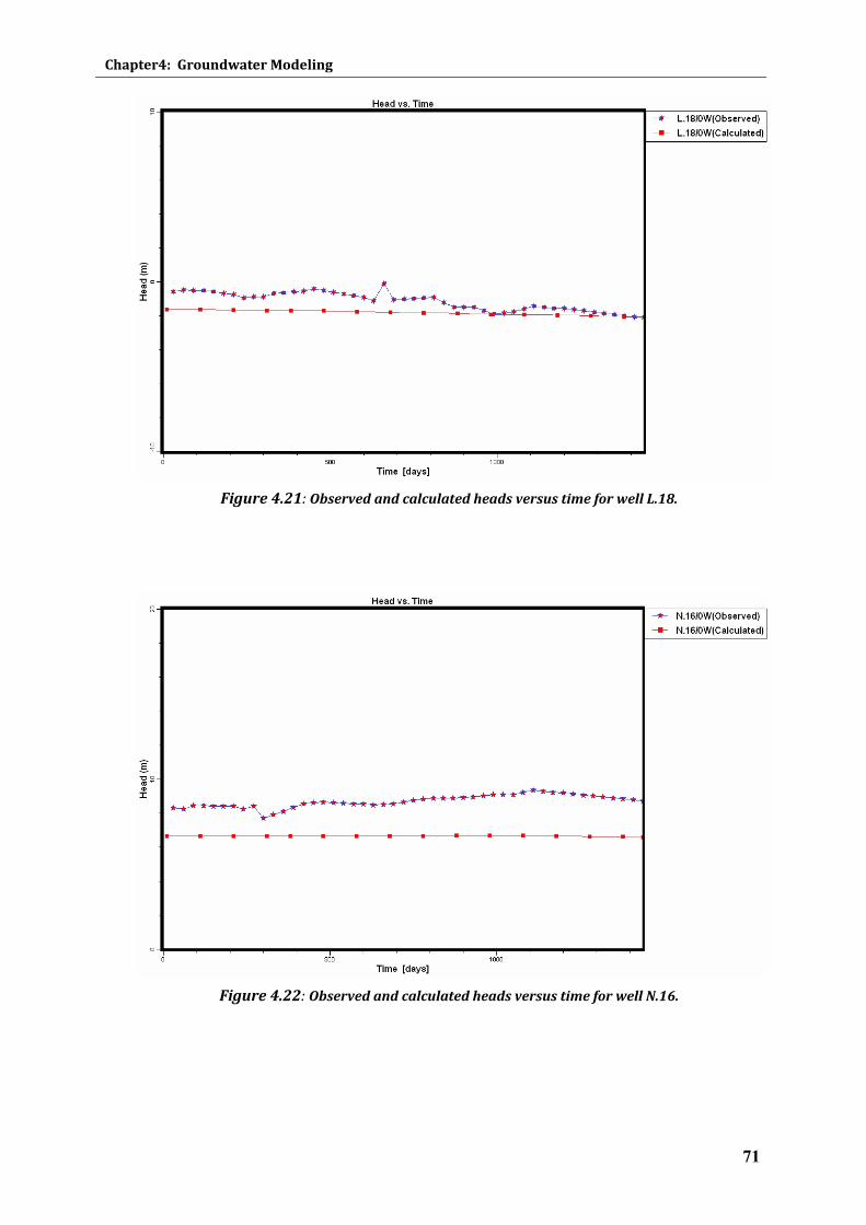
Chapter4: Groundwater Modeling
71
Figure 4.21: Observed and calculated heads versus time for well L.18.
Figure 4.22: Observed and calculated heads versus time for well N.16.
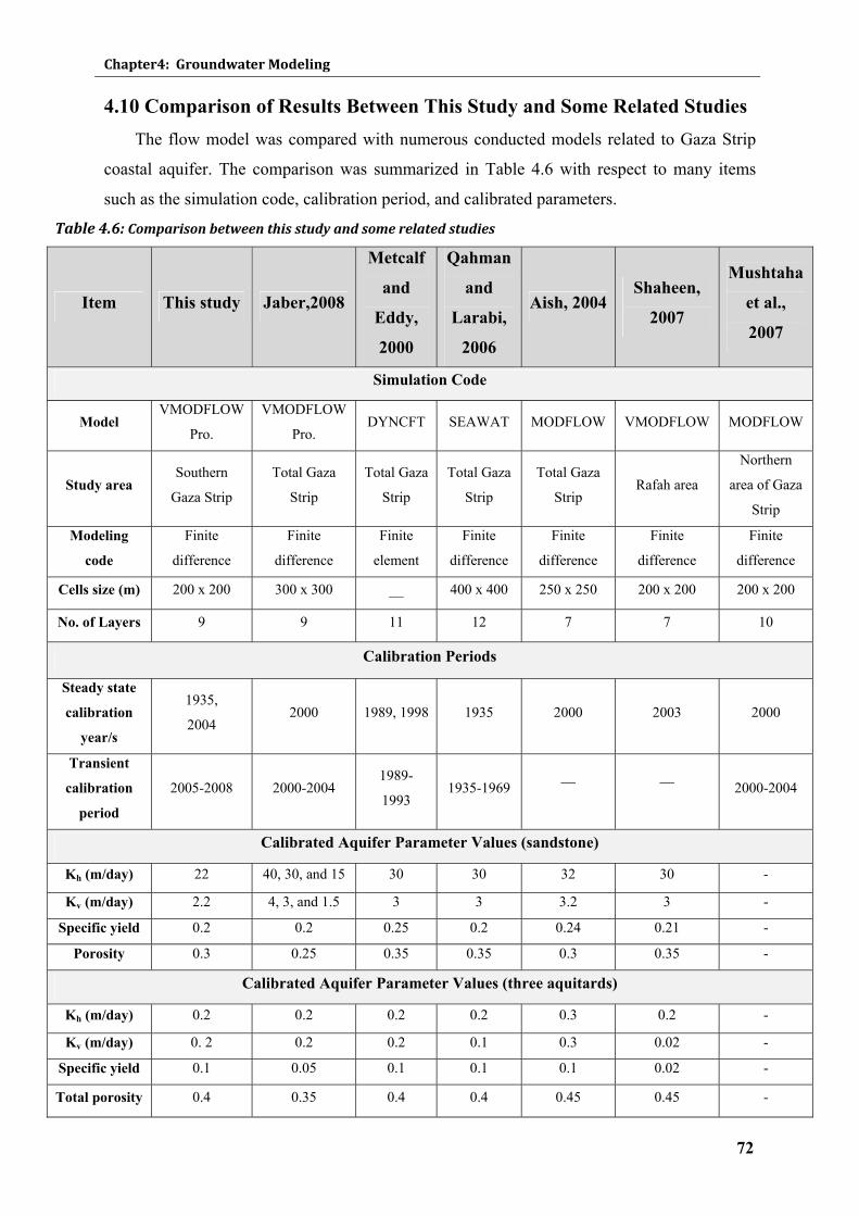
Chapter4: Groundwater Modeling
72
4.10 Comparison of Results Between This Study and Some Related Studies The flow model was compared with numerous conducted models related to Gaza Strip
coastal aquifer. The comparison was summarized in Table 4.6 with respect to many items
such as the simulation code, calibration period, and calibrated parameters.
Table 4.6: Comparison between this study and some related studies
Item This study Jaber,2008
Metcalf
and
Eddy,
2000
Qahman
and
Larabi,
2006
Aish, 2004Shaheen,
2007
Mushtaha
et al.,
2007
Simulation Code
Model VMODFLOW
Pro.
VMODFLOW
Pro. DYNCFT SEAWAT MODFLOW VMODFLOW MODFLOW
Study area Southern
Gaza Strip
Total Gaza
Strip
Total Gaza
Strip
Total Gaza
Strip
Total Gaza
Strip Rafah area
Northern
area of Gaza
Strip
Modeling
code
Finite
difference
Finite
difference
Finite
element
Finite
difference
Finite
difference
Finite
difference
Finite
difference
Cells size (m) 200 x 200 300 x 300 __ 400 x 400 250 x 250 200 x 200 200 x 200
No. of Layers 9 9 11 12 7 7 10
Calibration Periods
Steady state
calibration
year/s
1935,
2004 2000 1989, 1998 1935 2000 2003 2000
Transient
calibration
period
2005-2008 2000-2004 1989-
1993 1935-1969
__
__
2000-2004
Calibrated Aquifer Parameter Values (sandstone)
Kh (m/day) 22 40, 30, and 15 30 30 32 30 -
Kv (m/day) 2.2 4, 3, and 1.5 3 3 3.2 3 -
Specific yield 0.2 0.2 0.25 0.2 0.24 0.21 -
Porosity 0.3 0.25 0.35 0.35 0.3 0.35 -
Calibrated Aquifer Parameter Values (three aquitards)
Kh (m/day) 0.2 0.2 0.2 0.2 0.3 0.2 -
Kv (m/day) 0. 2 0.2 0.2 0.1 0.3 0.02 -
Specific yield 0.1 0.05 0.1 0.1 0.1 0.02 -
Total porosity 0.4 0.35 0.4 0.4 0.45 0.45 -
Chapter4: Groundwater Modeling
73
4.11 Transport Model The solute transport model describes the process of advection, dispersion-diffusion and
chemical reactions. The model set-up was conducted based on the results of the flow model.
Transport model was checked for both steady state flow and transient flow conditions. The
main transport calibrated parameter was dispersivity.
4.11.1 Assumptions for the Transport Model
o All the calibrated physical and hydro-geological parameters of the aquifer were kept
the same as in the baseline model in the previous (flow model).
o The same nitrate load was kept during all simulation transport periods (as calculated
in Appendix A). Therefore, it was expected to see increasing of nitrate concentration
year after year in all areas where the nitrate load exists. Actually, this is not the
situation in Gaza because the previous studies showed that there were three trend
types of groundwater quality ranging from decreasing (2%), constant (67%) to
increasing (31%) of observation points in the period between 1980 and 2002, (Al
Mahallawi, 2005).
o Zero nitrate concentration of the lateral inflow from the eastern borders of southern
Gaza Strip as explained before. Of course, the groundwater flowing from east and
entering the system contains nitrate, but we assumed low concentration so it can be
neglected.
o Natural precipitation & atmospheric deposition were ignored.
o Transformation of nitrogen forms in the unsaturated zone above water table is not
considered in details in this research, because there is a wide variability in the
conditions that control the mechanisms of each process, i.e. nitrification,
denitrification…..etc. Accurate determination of the contribution of each process in
the mass of nitrate reaching the water table is very difficult and many parameters are
needed, which are not available in Gaza due to the lack of data specially laboratory
measurements.
o Initial concentrations of the transport model under transient state groundwater flow
conditions (2005-2008) were set as the observed concentrations of nitrate in the model
area at the end of year 2004.
4.11.2 Calibration of Transport Model
The process of calibration requires adjustments of the model input parameters that
influence the output in MT3D are specially the recharge concentration value and the
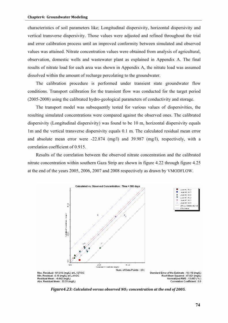
Chapter4: Groundwater Modeling
74
characteristics of soil parameters like; Longitudinal dispersivity, horizontal dispersivity and
vertical transverse dispersivity. Those values were adjusted and refined throughout the trial
and error calibration process until an improved conformity between simulated and observed
values was attained. Nitrate concentration values were obtained from analysis of agricultural,
observation, domestic wells and wastewater plant as explained in Appendix A. The final
results of nitrate load for each area was shown in Appendix A, the nitrate load was assumed
dissolved within the amount of recharge percolating to the groundwater.
The calibration procedure is performed under transient state groundwater flow
conditions. Transport calibration for the transient flow was conducted for the target period
(2005-2008) using the calibrated hydro-geological parameters of conductivity and storage.
The transport model was subsequently tested for various values of dispersivities, the
resulting simulated concentrations were compared against the observed ones. The calibrated
dispersivity (Longitudinal dispersivity) was found to be 10 m, horizontal dispersivity equals
1m and the vertical transverse dispersivity equals 0.1 m. The calculated residual mean error
and absolute mean error were -22.874 (mg/l) and 39.987 (mg/l), respectively, with a
correlation coefficient of 0.915.
Results of the correlation between the observed nitrate concentration and the calibrated
nitrate concentration within southern Gaza Strip are shown in figure 4.22 through figure 4.25
at the end of the years 2005, 2006, 2007 and 2008 respectively as drawn by VMODFLOW.
Figure4.23: Calculated versus observed NO3 concentration at the end of 2005.
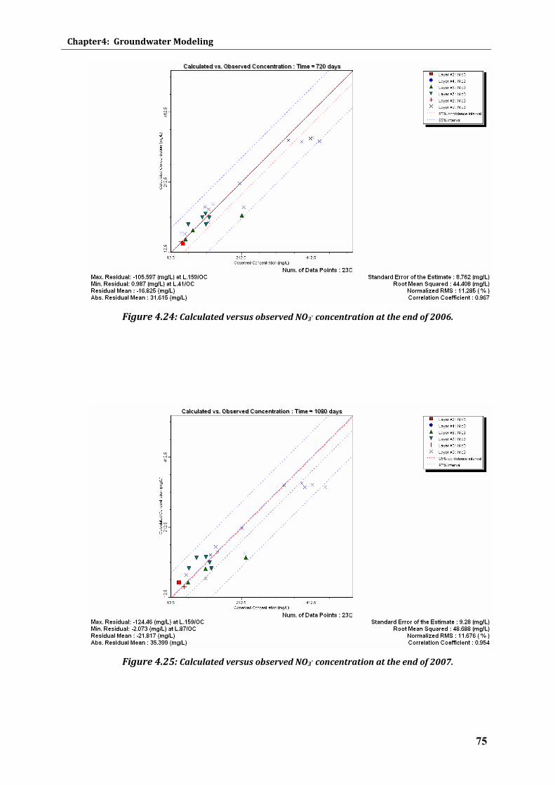
Chapter4: Groundwater Modeling
75
Figure 4.24: Calculated versus observed NO3 concentration at the end of 2006.
Figure 4.25: Calculated versus observed NO3 concentration at the end of 2007.
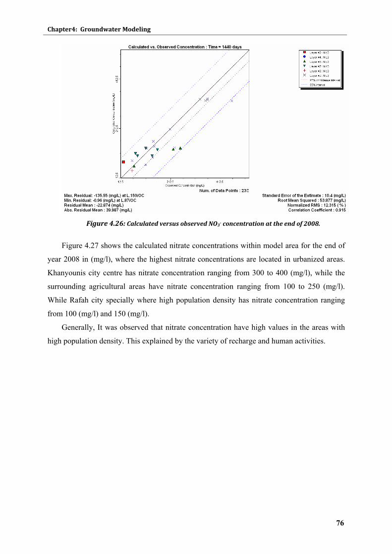
Chapter4: Groundwater Modeling
76
Figure 4.26: Calculated versus observed NO3 concentration at the end of 2008.
Figure 4.27 shows the calculated nitrate concentrations within model area for the end of
year 2008 in (mg/l), where the highest nitrate concentrations are located in urbanized areas.
Khanyounis city centre has nitrate concentration ranging from 300 to 400 (mg/l), while the
surrounding agricultural areas have nitrate concentration ranging from 100 to 250 (mg/l).
While Rafah city specially where high population density has nitrate concentration ranging
from 100 (mg/l) and 150 (mg/l).
Generally, It was observed that nitrate concentration have high values in the areas with
high population density. This explained by the variety of recharge and human activities.
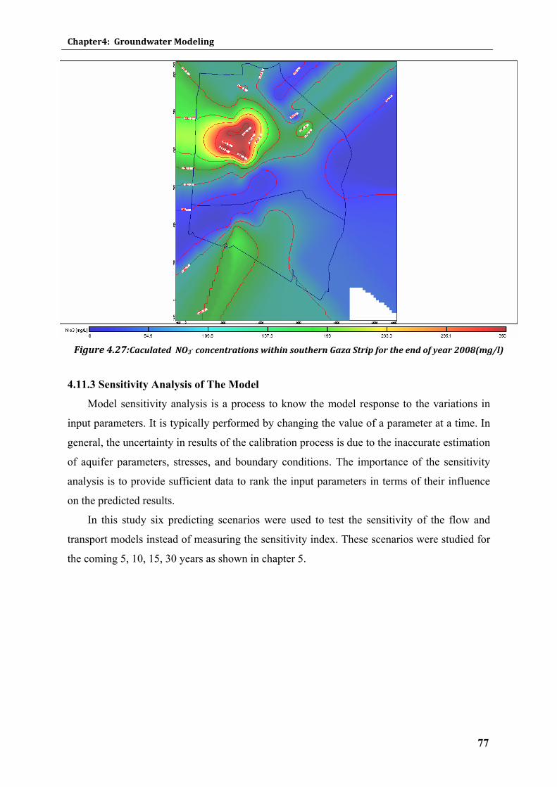
Chapter4: Groundwater Modeling
77
Figure 4.27:Caculated NO3 concentrations within southern Gaza Strip for the end of year 2008(mg/l)
4.11.3 Sensitivity Analysis of The Model
Model sensitivity analysis is a process to know the model response to the variations in
input parameters. It is typically performed by changing the value of a parameter at a time. In
general, the uncertainty in results of the calibration process is due to the inaccurate estimation
of aquifer parameters, stresses, and boundary conditions. The importance of the sensitivity
analysis is to provide sufficient data to rank the input parameters in terms of their influence
on the predicted results.
In this study six predicting scenarios were used to test the sensitivity of the flow and
transport models instead of measuring the sensitivity index. These scenarios were studied for
the coming 5, 10, 15, 30 years as shown in chapter 5.
Chapter5: Management Scenarios
78
CHAPTER 5
MANAGEMENT
SCENARIOS
Chapter5: Management Scenarios
79
CHAPTER 5: MANAGEMENT SCENARIOS
5.1 Introduction The advantage of a calibrated ground water model is that it can be applied to investigate
'what -if' scenarios and answer planning questions and predict impact of aquifer management
decisions (Metcalf and Eddy, 2000). The management options or scenarios may be regional-
scale approaches or local- scale scenarios. In this study only the local- scale scenarios were
studied.
There are many localized and specific management techniques can be investigated. The
management options were tested with the calibrated, coupled flow and transport model. It
should be noticed that all scenarios focused on Khanyounis area within the model
domain, whereby the research aimed in all to find a reliable solution of the nitrate
contamination in Khanyounis. The approach for selecting the management scenarios was
carried out depending on the need to reduce the migration of nitrate into the aquifer
system, and, according to the results of transport model. All alternatives of scenarios
based on management the pumping from the aquifer and management the land use
especially which effects on nitrate concentration. It is difficult to enumerate all available
and feasible alternatives to protect the aquifer against deterioration of water quality with
respect to nitrate. Six selected management scenarios were tested; (1) work as usual (zero
scenario), (2) Management of the pumping, (3) Implementation of sewerage system at
Khanyounis, (4) Reduction of N-fertilizers loadings at agricultural areas, (5) Bringing
together all the previous scenarios (2,3,and 4) and (6) Using artificial infiltration of
groundwater in addition to the management options in scenario no. (5). All scenarios
were studied for the coming 5, 10, 15, 30 years.
5.2 Management Scenarios This section aims to identify the future extent and the long-term trends in groundwater
concentrations for the target period (2009-2038) when applying the suggested management
scenarios. For the scenario analysis, all calibrated physical and hydro-geological parameters
from the flow model were used. Also, the calibrated yearly nitrate load presented in the
previous chapter was kept the same as the baseline to predict the future nitrate. As shown in
the previous section the six management scenarios were tested in this study were:
(1) Work as usual (zero scenario),
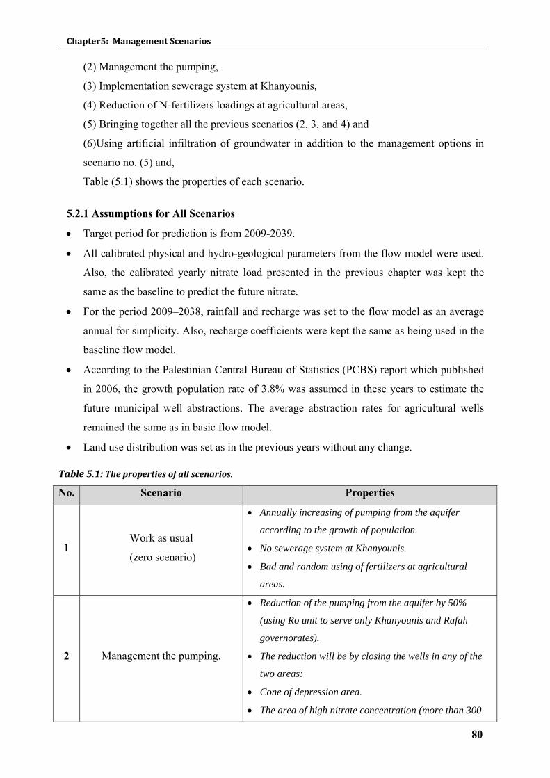
Chapter5: Management Scenarios
80
(2) Management the pumping,
(3) Implementation sewerage system at Khanyounis,
(4) Reduction of N-fertilizers loadings at agricultural areas,
(5) Bringing together all the previous scenarios (2, 3, and 4) and
(6)Using artificial infiltration of groundwater in addition to the management options in
scenario no. (5) and,
Table (5.1) shows the properties of each scenario.
5.2.1 Assumptions for All Scenarios
• Target period for prediction is from 2009-2039.
• All calibrated physical and hydro-geological parameters from the flow model were used.
Also, the calibrated yearly nitrate load presented in the previous chapter was kept the
same as the baseline to predict the future nitrate.
• For the period 2009–2038, rainfall and recharge was set to the flow model as an average
annual for simplicity. Also, recharge coefficients were kept the same as being used in the
baseline flow model.
• According to the Palestinian Central Bureau of Statistics (PCBS) report which published
in 2006, the growth population rate of 3.8% was assumed in these years to estimate the
future municipal well abstractions. The average abstraction rates for agricultural wells
remained the same as in basic flow model.
• Land use distribution was set as in the previous years without any change.
Table 5.1: The properties of all scenarios.
No. Scenario Properties
1 Work as usual
(zero scenario)
• Annually increasing of pumping from the aquifer
according to the growth of population.
• No sewerage system at Khanyounis.
• Bad and random using of fertilizers at agricultural
areas.
2 Management the pumping.
• Reduction of the pumping from the aquifer by 50%
(using Ro unit to serve only Khanyounis and Rafah
governorates).
• The reduction will be by closing the wells in any of the
two areas:
• Cone of depression area.
• The area of high nitrate concentration (more than 300
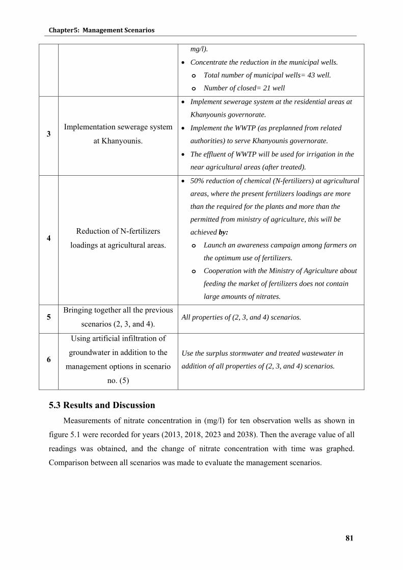
Chapter5: Management Scenarios
81
mg/l).
• Concentrate the reduction in the municipal wells.
o Total number of municipal wells= 43 well.
o Number of closed= 21 well
3 Implementation sewerage system
at Khanyounis.
• Implement sewerage system at the residential areas at
Khanyounis governorate.
• Implement the WWTP (as preplanned from related
authorities) to serve Khanyounis governorate.
• The effluent of WWTP will be used for irrigation in the
near agricultural areas (after treated).
4 Reduction of N-fertilizers
loadings at agricultural areas.
• 50% reduction of chemical (N-fertilizers) at agricultural
areas, where the present fertilizers loadings are more
than the required for the plants and more than the
permitted from ministry of agriculture, this will be
achieved by:
o Launch an awareness campaign among farmers on
the optimum use of fertilizers.
o Cooperation with the Ministry of Agriculture about
feeding the market of fertilizers does not contain
large amounts of nitrates.
5 Bringing together all the previous
scenarios (2, 3, and 4). All properties of (2, 3, and 4) scenarios.
6
Using artificial infiltration of
groundwater in addition to the
management options in scenario
no. (5)
Use the surplus stormwater and treated wastewater in
addition of all properties of (2, 3, and 4) scenarios.
5.3 Results and Discussion Measurements of nitrate concentration in (mg/l) for ten observation wells as shown in
figure 5.1 were recorded for years (2013, 2018, 2023 and 2038). Then the average value of all
readings was obtained, and the change of nitrate concentration with time was graphed.
Comparison between all scenarios was made to evaluate the management scenarios.
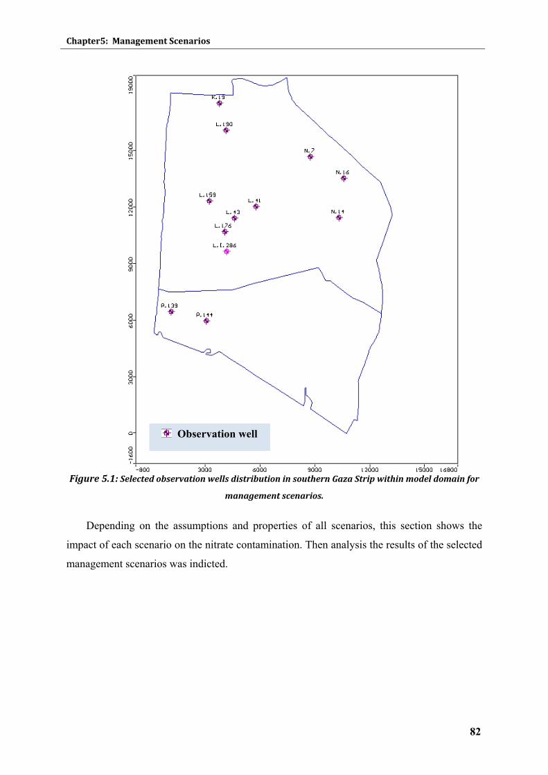
Chapter5: Management Scenarios
82
Figure 5.1: Selected observation wells distribution in southern Gaza Strip within model domain for
management scenarios.
Depending on the assumptions and properties of all scenarios, this section shows the
impact of each scenario on the nitrate contamination. Then analysis the results of the selected
management scenarios was indicted.
Observation well
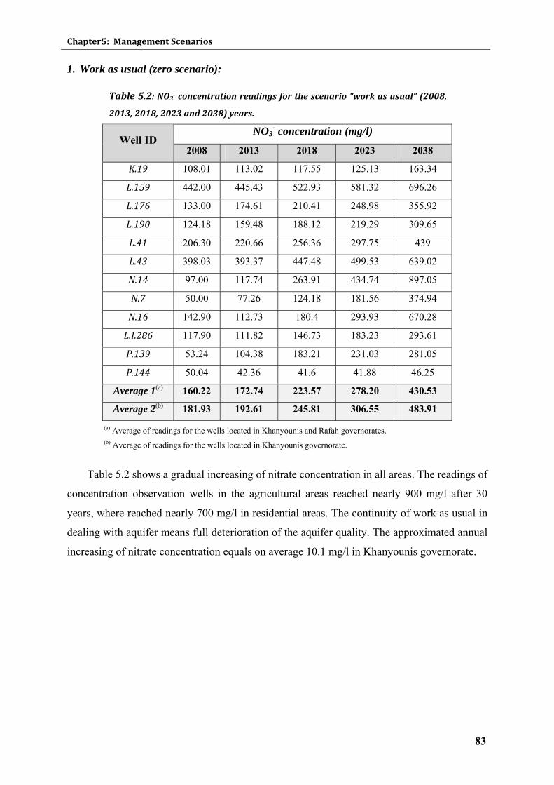
Chapter5: Management Scenarios
83
1. Work as usual (zero scenario):
Table 5.2: NO3 concentration readings for the scenario "work as usual" (2008,
2013, 2018, 2023 and 2038) years.
NO3- concentration (mg/l)
Well ID 2008 2013 2018 2023 2038
K.19 108.01 113.02 117.55 125.13 163.34
L.159 442.00 445.43 522.93 581.32 696.26
L.176 133.00 174.61 210.41 248.98 355.92
L.190 124.18 159.48 188.12 219.29 309.65
L.41 206.30 220.66 256.36 297.75 439
L.43 398.03 393.37 447.48 499.53 639.02
N.14 97.00 117.74 263.91 434.74 897.05
N.7 50.00 77.26 124.18 181.56 374.94
N.16 142.90 112.73 180.4 293.93 670.28
L.I.286 117.90 111.82 146.73 183.23 293.61
P.139 53.24 104.38 183.21 231.03 281.05
P.144 50.04 42.36 41.6 41.88 46.25
Average 1(a) 160.22 172.74 223.57 278.20 430.53
Average 2(b) 181.93 192.61 245.81 306.55 483.91
(a) Average of readings for the wells located in Khanyounis and Rafah governorates. (b) Average of readings for the wells located in Khanyounis governorate.
Table 5.2 shows a gradual increasing of nitrate concentration in all areas. The readings of
concentration observation wells in the agricultural areas reached nearly 900 mg/l after 30
years, where reached nearly 700 mg/l in residential areas. The continuity of work as usual in
dealing with aquifer means full deterioration of the aquifer quality. The approximated annual
increasing of nitrate concentration equals on average 10.1 mg/l in Khanyounis governorate.
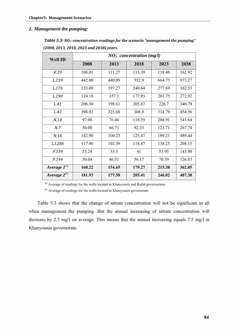
Chapter5: Management Scenarios
84
2. Management the pumping:
Table 5.3: NO3 concentration readings for the scenario "management the pumping"
(2008, 2013, 2018, 2023 and 2038) years.
NO3-
concentration (mg/l) Well ID
2008 2013 2018 2023 2038
K.19 108.01 111.27 113.39 118.48 162.92
L.159 442.00 440.09 552.9 664.75 973.27
L.176 133.00 197.27 240.64 277.69 362.53
L.190 124.18 157.1 177.93 201.75 272.92
L.41 206.30 198.61 205.67 226.7 340.79
L.43 398.03 325.68 308.9 314.79 454.36
N.14 97.00 76.46 118.39 204.91 541.64
N.7 50.00 66.71 92.33 123.71 267.74
N.16 142.90 100.25 125.47 189.21 489.44
L.I.286 117.90 102.39 118.47 138.25 208.15
P.139 53.24 33.5 41 53.95 143.98
P.144 50.04 46.51 56.17 70.39 126.83
Average 1(a) 160.22 154.65 179.27 215.38 362.05
Average 2(b) 181.93 177.58 205.41 246.02 407.38
(a) Average of readings for the wells located in Khanyounis and Rafah governorates. (b) Average of readings for the wells located in Khanyounis governorate.
Table 5.3 shows that the change of nitrate concentration will not be significant in all
when management the pumping. But the annual increasing of nitrate concentration will
decrease by 2.5 mg/l on average. This means that the annual increasing equals 7.5 mg/l in
Khanyounis governorate.
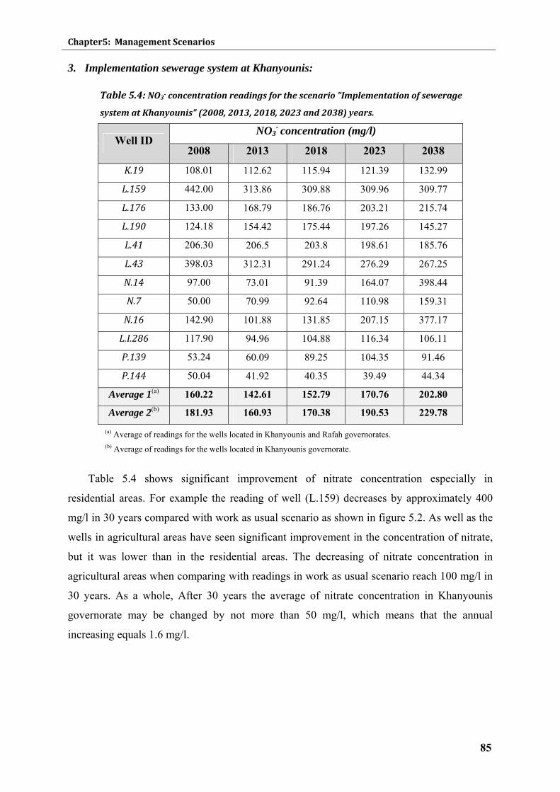
Chapter5: Management Scenarios
85
3. Implementation sewerage system at Khanyounis:
Table 5.4: NO3 concentration readings for the scenario "Implementation of sewerage
system at Khanyounis" (2008, 2013, 2018, 2023 and 2038) years.
NO3- concentration (mg/l)
Well ID 2008 2013 2018 2023 2038
K.19 108.01 112.62 115.94 121.39 132.99
L.159 442.00 313.86 309.88 309.96 309.77
L.176 133.00 168.79 186.76 203.21 215.74
L.190 124.18 154.42 175.44 197.26 145.27
L.41 206.30 206.5 203.8 198.61 185.76
L.43 398.03 312.31 291.24 276.29 267.25
N.14 97.00 73.01 91.39 164.07 398.44
N.7 50.00 70.99 92.64 110.98 159.31
N.16 142.90 101.88 131.85 207.15 377.17
L.I.286 117.90 94.96 104.88 116.34 106.11
P.139 53.24 60.09 89.25 104.35 91.46
P.144 50.04 41.92 40.35 39.49 44.34
Average 1(a) 160.22 142.61 152.79 170.76 202.80
Average 2(b) 181.93 160.93 170.38 190.53 229.78
(a) Average of readings for the wells located in Khanyounis and Rafah governorates. (b) Average of readings for the wells located in Khanyounis governorate.
Table 5.4 shows significant improvement of nitrate concentration especially in
residential areas. For example the reading of well (L.159) decreases by approximately 400
mg/l in 30 years compared with work as usual scenario as shown in figure 5.2. As well as the
wells in agricultural areas have seen significant improvement in the concentration of nitrate,
but it was lower than in the residential areas. The decreasing of nitrate concentration in
agricultural areas when comparing with readings in work as usual scenario reach 100 mg/l in
30 years. As a whole, After 30 years the average of nitrate concentration in Khanyounis
governorate may be changed by not more than 50 mg/l, which means that the annual
increasing equals 1.6 mg/l.
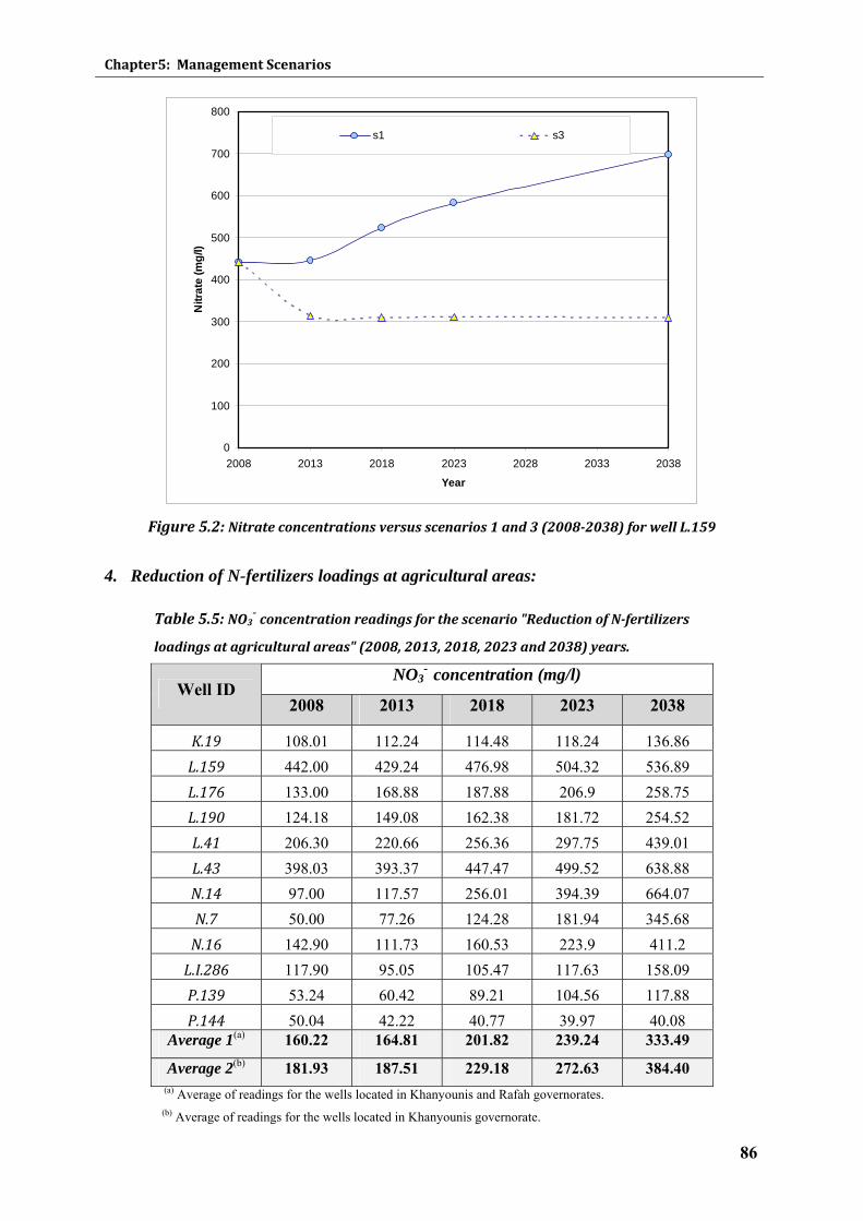
Chapter5: Management Scenarios
86
0
100
200
300
400
500
600
700
800
2008 2013 2018 2023 2028 2033 2038
Year
Nitr
ate
(mg/
l)
s1 s3
Figure 5.2: Nitrate concentrations versus scenarios 1 and 3 (20082038) for well L.159
4. Reduction of N-fertilizers loadings at agricultural areas:
Table 5.5: NO3- concentration readings for the scenario "Reduction of Nfertilizers
loadings at agricultural areas" (2008, 2013, 2018, 2023 and 2038) years.
NO3-
concentration (mg/l) Well ID
2008 2013 2018 2023 2038
K.19 108.01 112.24 114.48 118.24 136.86 L.159 442.00 429.24 476.98 504.32 536.89 L.176 133.00 168.88 187.88 206.9 258.75 L.190 124.18 149.08 162.38 181.72 254.52 L.41 206.30 220.66 256.36 297.75 439.01 L.43 398.03 393.37 447.47 499.52 638.88 N.14 97.00 117.57 256.01 394.39 664.07 N.7 50.00 77.26 124.28 181.94 345.68 N.16 142.90 111.73 160.53 223.9 411.2 L.I.286 117.90 95.05 105.47 117.63 158.09 P.139 53.24 60.42 89.21 104.56 117.88 P.144 50.04 42.22 40.77 39.97 40.08
Average 1(a) 160.22 164.81 201.82 239.24 333.49
Average 2(b) 181.93 187.51 229.18 272.63 384.40 (a) Average of readings for the wells located in Khanyounis and Rafah governorates. (b) Average of readings for the wells located in Khanyounis governorate.
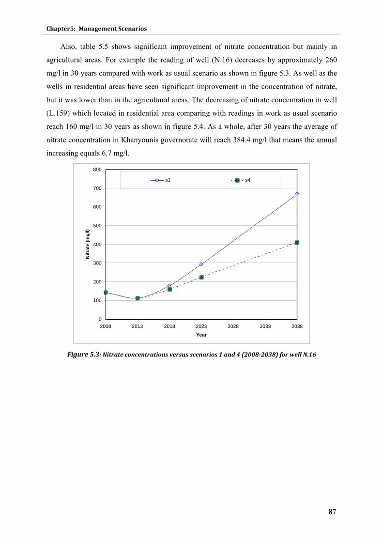
Chapter5: Management Scenarios
87
Also, table 5.5 shows significant improvement of nitrate concentration but mainly in
agricultural areas. For example the reading of well (N.16) decreases by approximately 260
mg/l in 30 years compared with work as usual scenario as shown in figure 5.3. As well as the
wells in residential areas have seen significant improvement in the concentration of nitrate,
but it was lower than in the agricultural areas. The decreasing of nitrate concentration in well
(L.159) which located in residential area comparing with readings in work as usual scenario
reach 160 mg/l in 30 years as shown in figure 5.4. As a whole, after 30 years the average of
nitrate concentration in Khanyounis governorate will reach 384.4 mg/l that means the annual
increasing equals 6.7 mg/l.
0
100
200
300
400
500
600
700
800
2008 2013 2018 2023 2028 2033 2038
Year
Nitr
ate
(mg/
l)
s1 s4
Figure 5.3: Nitrate concentrations versus scenarios 1 and 4 (20082038) for well N.16
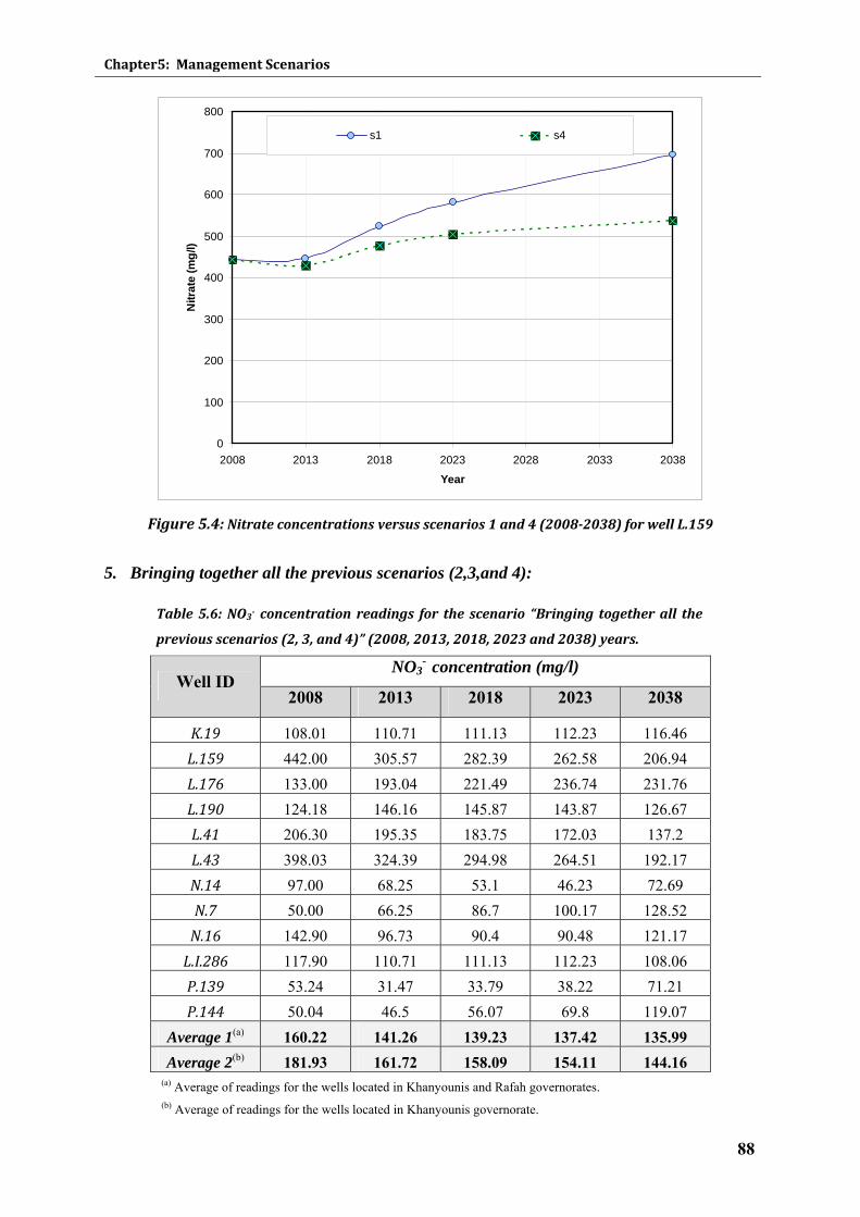
Chapter5: Management Scenarios
88
0
100
200
300
400
500
600
700
800
2008 2013 2018 2023 2028 2033 2038
Year
Nitr
ate
(mg/
l)
s1 s4
Figure 5.4: Nitrate concentrations versus scenarios 1 and 4 (20082038) for well L.159
5. Bringing together all the previous scenarios (2,3,and 4):
Table 5.6: NO3 concentration readings for the scenario “Bringing together all the
previous scenarios (2, 3, and 4)” (2008, 2013, 2018, 2023 and 2038) years.
NO3-
concentration (mg/l) Well ID
2008 2013 2018 2023 2038
K.19 108.01 110.71 111.13 112.23 116.46 L.159 442.00 305.57 282.39 262.58 206.94 L.176 133.00 193.04 221.49 236.74 231.76 L.190 124.18 146.16 145.87 143.87 126.67 L.41 206.30 195.35 183.75 172.03 137.2 L.43 398.03 324.39 294.98 264.51 192.17 N.14 97.00 68.25 53.1 46.23 72.69 N.7 50.00 66.25 86.7 100.17 128.52 N.16 142.90 96.73 90.4 90.48 121.17 L.I.286 117.90 110.71 111.13 112.23 108.06 P.139 53.24 31.47 33.79 38.22 71.21 P.144 50.04 46.5 56.07 69.8 119.07
Average 1(a) 160.22 141.26 139.23 137.42 135.99 Average 2(b) 181.93 161.72 158.09 154.11 144.16
(a) Average of readings for the wells located in Khanyounis and Rafah governorates. (b) Average of readings for the wells located in Khanyounis governorate.
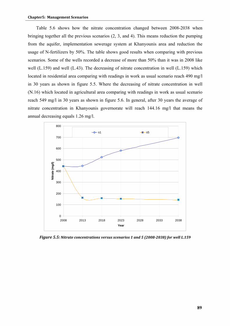
Chapter5: Management Scenarios
89
Table 5.6 shows how the nitrate concentration changed between 2008-2038 when
bringing together all the previous scenarios (2, 3, and 4). This means reduction the pumping
from the aquifer, implementation sewerage system at Khanyounis area and reduction the
usage of N-fertilizers by 50%. The table shows good results when comparing with previous
scenarios. Some of the wells recorded a decrease of more than 50% than it was in 2008 like
well (L.159) and well (L.43). The decreasing of nitrate concentration in well (L.159) which
located in residential area comparing with readings in work as usual scenario reach 490 mg/l
in 30 years as shown in figure 5.5. Where the decreasing of nitrate concentration in well
(N.16) which located in agricultural area comparing with readings in work as usual scenario
reach 549 mg/l in 30 years as shown in figure 5.6. In general, after 30 years the average of
nitrate concentration in Khanyounis governorate will reach 144.16 mg/l that means the
annual decreasing equals 1.26 mg/l.
0
100
200
300
400
500
600
700
800
2008 2013 2018 2023 2028 2033 2038
Year
Nitr
ate
(mg/
l)
s1 s5
Figure 5.5: Nitrate concentrations versus scenarios 1 and 5 (20082038) for well L.159
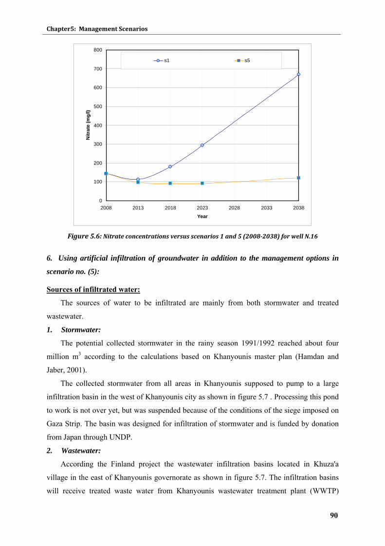
Chapter5: Management Scenarios
90
0
100
200
300
400
500
600
700
800
2008 2013 2018 2023 2028 2033 2038
Year
Nitr
ate
(mg/
l)
s1 s5
Figure 5.6: Nitrate concentrations versus scenarios 1 and 5 (20082038) for well N.16
6. Using artificial infiltration of groundwater in addition to the management options in
scenario no. (5):
Sources of infiltrated water:
The sources of water to be infiltrated are mainly from both stormwater and treated
wastewater.
1. Stormwater:
The potential collected stormwater in the rainy season 1991/1992 reached about four
million m3 according to the calculations based on Khanyounis master plan (Hamdan and
Jaber, 2001).
The collected stormwater from all areas in Khanyounis supposed to pump to a large
infiltration basin in the west of Khanyounis city as shown in figure 5.7 . Processing this pond
to work is not over yet, but was suspended because of the conditions of the siege imposed on
Gaza Strip. The basin was designed for infiltration of stormwater and is funded by donation
from Japan through UNDP.
2. Wastewater:
According the Finland project the wastewater infiltration basins located in Khuza'a
village in the east of Khanyounis governorate as shown in figure 5.7. The infiltration basins
will receive treated waste water from Khanyounis wastewater treatment plant (WWTP)
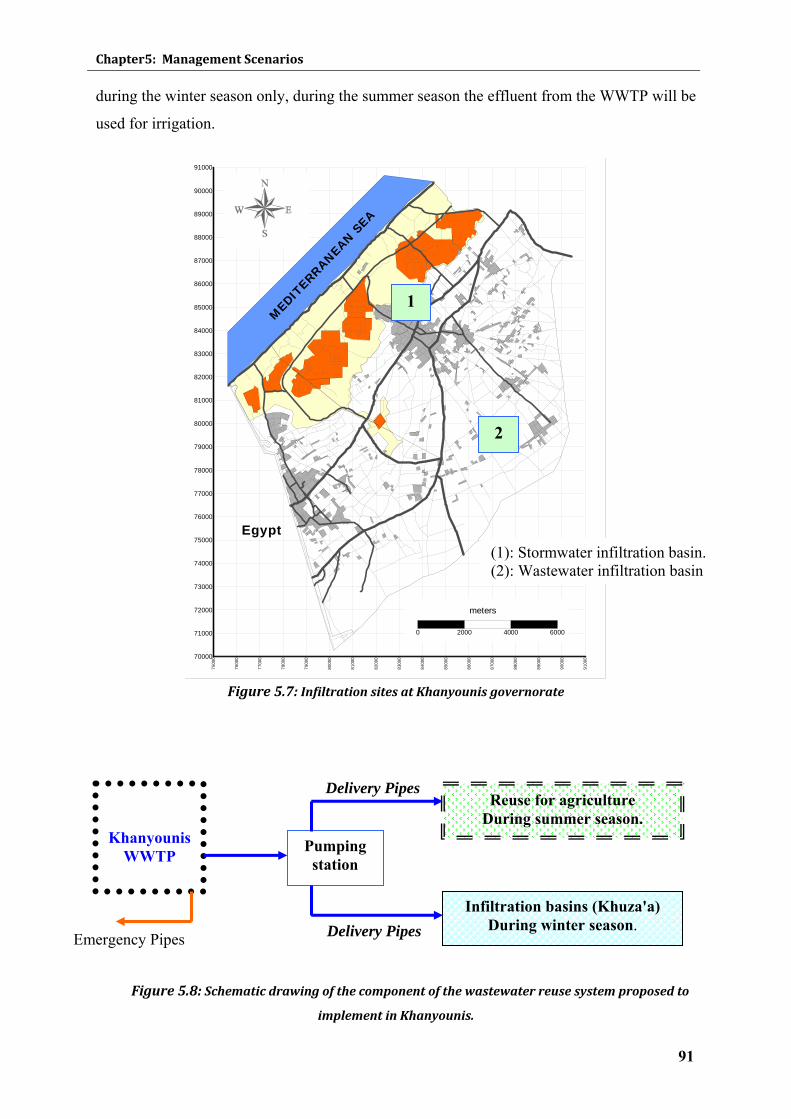
Chapter5: Management Scenarios
91
during the winter season only, during the summer season the effluent from the WWTP will be
used for irrigation.
7500
0
7600
0
7700
0
7800
0
7900
0
8000
0
8100
0
8200
0
8300
0
8400
0
8500
0
8600
0
8700
0
8800
0
8900
0
9000
0
9100
070000
71000
72000
73000
74000
75000
76000
77000
78000
79000
80000
81000
82000
83000
84000
85000
86000
87000
88000
89000
90000
91000
MEDIT
ERRANEAN S
EA
Egypt
meters
0 2000 4000 6000
Figure 5.7: Infiltration sites at Khanyounis governorate
Figure 5.8: Schematic drawing of the component of the wastewater reuse system proposed to
implement in Khanyounis.
2
1
(1): Stormwater infiltration basin. (2): Wastewater infiltration basin
Khanyounis WWTP Pumping
station
Infiltration basins (Khuza'a) During winter season.
Reuse for agriculture During summer season.
Delivery Pipes Emergency Pipes
Delivery Pipes
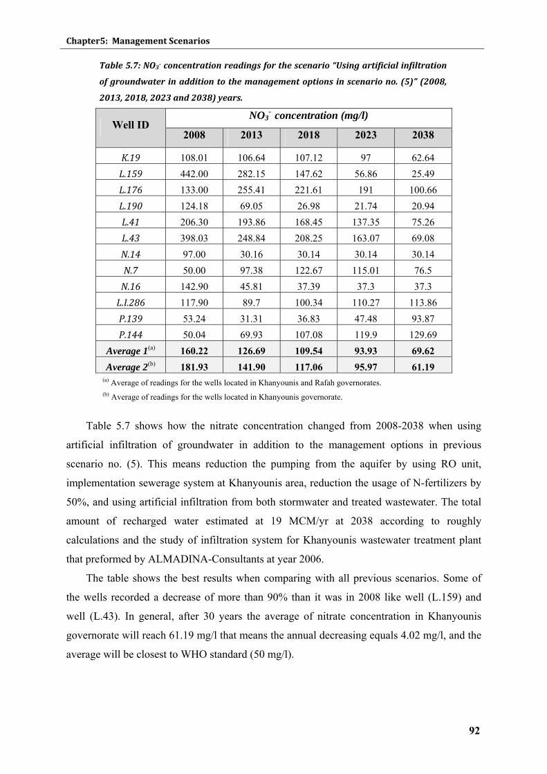
Chapter5: Management Scenarios
92
Table 5.7: NO3 concentration readings for the scenario “Using artificial infiltration
of groundwater in addition to the management options in scenario no. (5)” (2008,
2013, 2018, 2023 and 2038) years.
NO3-
concentration (mg/l) Well ID
2008 2013 2018 2023 2038
K.19 108.01 106.64 107.12 97 62.64 L.159 442.00 282.15 147.62 56.86 25.49 L.176 133.00 255.41 221.61 191 100.66 L.190 124.18 69.05 26.98 21.74 20.94 L.41 206.30 193.86 168.45 137.35 75.26 L.43 398.03 248.84 208.25 163.07 69.08 N.14 97.00 30.16 30.14 30.14 30.14 N.7 50.00 97.38 122.67 115.01 76.5 N.16 142.90 45.81 37.39 37.3 37.3 L.I.286 117.90 89.7 100.34 110.27 113.86 P.139 53.24 31.31 36.83 47.48 93.87 P.144 50.04 69.93 107.08 119.9 129.69
Average 1(a) 160.22 126.69 109.54 93.93 69.62 Average 2(b) 181.93 141.90 117.06 95.97 61.19
(a) Average of readings for the wells located in Khanyounis and Rafah governorates. (b) Average of readings for the wells located in Khanyounis governorate.
Table 5.7 shows how the nitrate concentration changed from 2008-2038 when using
artificial infiltration of groundwater in addition to the management options in previous
scenario no. (5). This means reduction the pumping from the aquifer by using RO unit,
implementation sewerage system at Khanyounis area, reduction the usage of N-fertilizers by
50%, and using artificial infiltration from both stormwater and treated wastewater. The total
amount of recharged water estimated at 19 MCM/yr at 2038 according to roughly
calculations and the study of infiltration system for Khanyounis wastewater treatment plant
that preformed by ALMADINA-Consultants at year 2006.
The table shows the best results when comparing with all previous scenarios. Some of
the wells recorded a decrease of more than 90% than it was in 2008 like well (L.159) and
well (L.43). In general, after 30 years the average of nitrate concentration in Khanyounis
governorate will reach 61.19 mg/l that means the annual decreasing equals 4.02 mg/l, and the
average will be closest to WHO standard (50 mg/l).
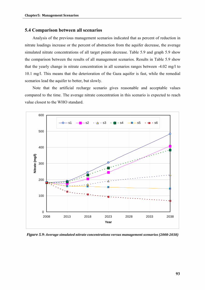
Chapter5: Management Scenarios
93
5.4 Comparison between all scenarios Analysis of the previous management scenarios indicated that as percent of reduction in
nitrate loadings increase or the percent of abstraction from the aquifer decrease, the average
simulated nitrate concentrations of all target points decrease. Table 5.9 and graph 5.9 show
the comparison between the results of all management scenarios. Results in Table 5.9 show
that the yearly change in nitrate concentration in all scenarios ranges between -4.02 mg/l to
10.1 mg/l. This means that the deterioration of the Gaza aquifer is fast, while the remedial
scenarios lead the aquifer to better, but slowly.
Note that the artificial recharge scenario gives reasonable and acceptable values
compared to the time. The average nitrate concentration in this scenario is expected to reach
value closest to the WHO standard.
0
100
200
300
400
500
600
2008 2013 2018 2023 2028 2033 2038
Year
Nitr
ate
(mg/
l)
s1 s2 s3 s4 s5 s6
Figure 5.9: Average simulated nitrate concentrations versus management scenarios (20082038)
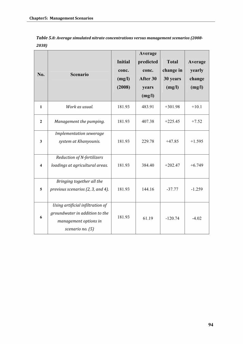
Chapter5: Management Scenarios
94
Table 5.8: Average simulated nitrate concentrations versus management scenarios (2008
2038)
No. Scenario
Initial
conc.
(mg/l)
(2008)
Average
predicted
conc.
After 30
years
(mg/l)
Total
change in
30 years
(mg/l)
Average
yearly
change
(mg/l)
1 Work as usual. 181.93 483.91 +301.98 +10.1
2 Management the pumping. 181.93 407.38 +225.45 +7.52
3
Implementation sewerage
system at Khanyounis.
181.93 229.78 +47.85 +1.595
4
Reduction of Nfertilizers
loadings at agricultural areas.
181.93 384.40 +202.47 +6.749
5
Bringing together all the
previous scenarios (2, 3, and 4).
181.93 144.16 -37.77 -1.259
6
Using artificial infiltration of
groundwater in addition to the
management options in
scenario no. (5)
181.93 61.19 -120.74 -4.02
Chapter6: Conclusion and recommendations
95
CHAPTER 6
CONCLUSION AND
RECOMMENDATIONS
Chapter6: Conclusion and recommendations
96
CHAPTER 6: CONCLUSION AND RECOMMENDATIONS
6.1 Conclusion
• The used finite-difference code MODFLOW to simulate the hydraulic head within the
groundwater and the MT3D to simulate the nitrate transport are good tools, meanwhile
other modeling tools may introduces better results than VMODFLOW.
• According to the management scenarios explained in chapter 5, Septic effluents are the
main sources of nitrate in the groundwater of Khanyounis governorate followed by
chemical fertilizers and manure.
• The abstraction from the aquifer affects on the nitrate concentration in groundwater.
Whenever the pumping from the aquifer increased the nitrate concentration increased,
the change is effective but not significant in comparing with annual increasing of nitrate
concentration. This relation may be due to change in direction and velocity of the flow of
groundwater, especially in the areas of cones of depression. Other factor may enhance
this relation is the significant change of aquifer storage.
• In the event of work as usual, the average nitrate concentration in Khanyounis
governorate will increases by more than 10 mg/l annually.
• The implementation a sewerage system at Khanyounis governorate will reduce the rising
of average nitrate concentration in Khanyounis area by 8.5 mg/l annually. This means
that the average nitrate concentration in Khanyounis governorate will increases by only
1.5 mg/l annually.
• Reduction of usage N-fertilizers by 50% will have somewhat effect on nitrate
concentration where it will reduce the rising of average nitrate concentration in
Khanyounis area by 3.35 mg/l annually.
• Combination of all management scenarios in addition to artificial recharge i.e. (reduction
the pumping from the aquifer by using RO unit, implementation sewerage system at
Khanyounis area, reduction the usage of N-fertilizers by 50%, and using artificial
infiltration from both stormwater and treated wastewater) will lead to acceptable nitrate
of concentration in groundwater after 30 years of applying these options.
• The analysis of the impact of projects planned to be implemented in the future by the
concerned authorities showed that these projects will have a positive impact in solving
the problem of nitrate in Khanyounis governorate. These projects include the
implementation of stormwater infiltration basin and wastewater infiltration basins.
Chapter6: Conclusion and recommendations
97
6.2 Recommendations 1. This study can be used as a guide to the concerned authorities and in charge of the
follow-up to the quality of groundwater. It introduced in numbers the effect of many
management options on nitrate concentration in Khanyounis governorate area.
2. The continuous deterioration of Gaza aquifer should be stopped. The management
options in this study help to stop the deterioration. It is the first step in management the
groundwater quality. The second step is to search for other sources of water from the
aquifer. Alternative sources can be plants for seawater desalination, imported water from
water companies as Mekorot, or other sources.
3. The implementation of Khanyounis WWTP and operation of its sewerage system will
help significantly in reducing the average nitrate concentration in this area.
4. Artificial infiltration from both stormwater and treated wastewater will have dramatic
effect on reducing nitrate concentration in groundwater.
5. The best scenario to solve the increasing of nitrate concentration problem in the
groundwater is the combination of many options (reduction the pumping from the aquifer
by using RO unit, implementation sewerage system at Khanyounis area, reduction the
usage of N-fertilizers by 50%, and using artificial infiltration from both stormwater and
treated wastewater) in addition to artificial recharge as planned by the concerned
authorities.
6. As a general recommendation, PWA, MoA, CMWU, and other related authorities has to
construct an integrated data base for hydrological data of Gaza Strip.
6.3 Suggested complementary studies 1. Studying the nitrate transport in the unsaturated zone, and finding empirical equations or
model to simplify the calculation of nitrate loads leaching to saturated zone.
2. Studying carefully the impact of artificial recharge on nitrate concentration in
groundwater in Khanyounis area.
3. Searching for another software to model the nitrate transport in groundwater.
References
98
REFERENCES
References
99
REFERENCES
1. Abu Maila Y, El-Nahal I and Al-Agha M.R, 2004. Seasonal variations and
mechanisms of groundwater nitrate pollution in the Gaza Strip. Gaza, Palestine.
2. Abu Naser AA, Ghbn N, Khoudary R, 2002. The relation of nitrate contamination of
groundwater with methaemoglobin level among infants in Gaza. Ministry of Health,
Gaza, Palestine.
3. Abushback T, 2006. The Effect of Soil Type and Wastewater Composition on the
Nitrification Denitrification Processes During Groundwater Recharge. This research
was funded by UNESCO-FLANDER FIT, Palestine. Contract No., Budget Code
513RAB2041.
4. Aish A, 2000. Nitrate Pollution and Contaminant Transport to Groundwater
Resources. M.Sc dissertation. Vrije Universiteit Brussels VUB, Belgium.
5. Aish A, 2004. Hydrogeological Study and Artificial Recharge Modeling of the Gaza
Coastal Aquifer Using GIS and MODFLOW. PhD Dissertation, Holland, Vrije
Universiteit Brussels VUB, Belgium.
6. Alawneh M, 1996. Nitrate formation and transport through sandy soils. M.Sc Thesis,
PP 2-8, IHE-DELFT
7. Al-Jamal K and AI-Yaqubi A, 2000. Sustainable Water Resources Management of
Gaza Coastal Aquifer. Palestinian Water Authority (PWA), Gaza, Palestinian.
8. ALMADINA-Consultants with the Finland Project Management Unit (PMU) in
PWA, 2006. Khanyounis wastewater treatment plant- Infiltration System-
Geotechnical and Hydrological Study. Gaza
9. Al Mahallawi K, 2005. Modeling interaction of land use, urbanization and
hydrological factors for the analysis of groundwater quality in Mediterranean zone
(Example the Gaza Strip, Palestine). PhD Dissertation, Lille, France, University of
Lille for science and technology.
10. Almasri M and Ghabayen S, 2007. Analysis of Nitrate Contamination of Gaza Coastal
Aquifer, Palestine. Gaza, Palestine.
11. Almasri M, Ghabayen S, Kaluarachchi J.J, Jarrar A, Jayyousi A and Mac McKee M,
2005. A Conceptual Framework for Managing Nitrate Contamination of the Gaza
Coastal Aquifer. EWRI Conference USA.
References
100
12. Almasri M, Kaluarachchi J.J, 2004a. Assessment and management of long-term
nitrate pollution of ground water in agriculture-dominated watersheds. Hydrology.
295: 225-245.
13. Almasri M, Kaluarachchi J.J, 2004b. Implications of on-ground nitrogen loading and
soil transformations on ground water quality management. Journal of the American
Water Resources Association
14. Almasri M, Kaluarachchi J.J, 2005. Modular neural networks to predict the nitrate
distribution in ground water using the on-ground nitrogen loading and recharge data.
Environmental Modelling & Software 20: 851-871.
15. Anderson M.P, and Woessner W.W, 1992. Applied groundwater modeling:
simulation of flow and advective transport. Academic Press, Inc.
16. BÖHLKE J.K, MICHALSKI Greg, Peter B, and DENSMORE Jill N, 2004. Sources
and isotopic characteristics of vadose-zone nitrate in arid regions. Denver Annual
Meeting (November 7–10, 2004).
17. Cabrera A and Blarasin M, 1999. Nitrate Contamination in the phreatic aquifer of an
agro ecosystem of the Chacopampeana plain, Cordoba, Argentina. Journal of
Environmental Hydrology 7: Paper 17.
18. Chowdary V.M, Rao N.H, Sarma P.B.S, 2005. Decision support framework for
assessment of non-point-source pollution of groundwater in large irrigation projects.
Agricultural Water Management 75: 194–225.
19. Clarke K, 1999. Getting started with geographic information systems. University of
California, Santa Barbara, Prentice Hall, New Jersey.
20. Daibes F, 2003. Water in Palestine Problems -Politics- Prospects. Jerusalem,
PASSIA.
21. De Smedt F, 2003. Groundwater modeling. Course notes.
22. Environmental Planning Directorate (EPD) in the Ministry of Planning, 1995. Study
on nitrate pollution in Gaza's groundwater. Gaza.
23. Hajhamad L, Almasri , 2009. Assessment of nitrate contamination of groundwater
using lumped-parameter models. Environmental Modeling & Software 24 (2009)
1073–1087.
24. Hamadan S, Jaber I, 2001. Artificial infiltration of groundwater- A tool towards the
sustainability of water resources in Gaza Strip. sixth international technology
conference, IWTC 2001, Alexandria, Egypt.
References
101
25. Harbaugh A, Banata E, Hill M, and McDonald M, 2000. The U.S. Geological survey
modular groundwater model-user gaudier to modularization concepts and the
groundwater flow process.
26. Harbaugh A, and McDonald M, 1996. User’s documentation for MODFLOW-96, an
update to the US Geological Survey modular finite difference groundwater flow
model. US Geological Survey.
27. Harbaugh A, and M McDonald, 1996. User's documentation for MODFLOW-96, an
update to the U.S. Geological Survey modular finite-difference ground-water model.
US Geological Survey. Open-File Rep. 96–485.
28. Jaber R, 2008. Fate and transport of the coastal aquifer of Gaza Strip and the feasible
management options. M.Sc Dissertation. Jordan University of Science and
Technology, Feb 2004.
29. Keeney D, 1989. Sources of nitrate to groundwater. In: R E Follet (ed). Nitrogen
management and groundwater protection. Elsevier, New York. P 23-32.
30. Khayat S, Geyer S, Hotzl H, Ghanem M, and Alia W, 2006. Identification of nitrate
sources in groundwater by nitrateN15δ and nitrateO18δ isotopes: a study of the shallow
Pleistocene aquifer in the Jericho area, Palestine. Wiley-VCH GmbH & Co. KGaA,
Weinheim.
31. Lake I, Lovett A, Hiscock K, Betson M, Foley A, Su¨nnenberg G, Evers S, Fletcher
S, 2003. Evaluating factors influencing groundwater vulnerability to nitrate pollution,
developing the potential of GIS. Journal of Environmental Management. 68: 315–328.
32. Legg J.O and J.J Meisinger, 1982. Soil Nitrogen Budgets. In F J Stevenson (ed).
Nitrogen in agricultural soils. Agron Monogr22. ASA, CSSA, and SSSA, and
Madison, WI. P 503-566.
33. Mcclain M, Richey J, Pimentel T. Groundwater nitrogen dynamics at the terrestrial-
lotic interface of a small catchment in the Central Amazon Basin. Biogeochem 1994;
27: 113-127.
34. Metcalf & Eddy, Inc.1990. Waste water Engineering. 3rd edition. NewYork:
McGraw-Hill.
35. Metcalf and Eddy, 2000. Coastal Aquifer Management Plan (CAMP). Final model
report (task 7). USAID, Contract No. 294-C-99-00038-00.
36. Meybeck M and Helmer R 1996. A Guide to the Use of Biota, Sediment and Water in
References
102
Environmental Monitoring. Second edition. Published on behalf of UNESCO, WHO
and UNEP by E&FN Spon, London, 1-57.
37. Mogheir Y, 2005. Spatial assessment and redesign of a groundwater quality
monitoring network using entropy theory, Gaza Strip, Palestine. Environment Quality
Authority, Gaza, Palestine.
38. Molenat J, Gascuel-Odoux C, 2002. Modeling flow and nitrate transport in
groundwater for the prediction of water travel times and of consequences of land use
evolution on water quality. Hydrogeological processes. 16: 479-492.
39. MOPIC, 1996. Gaza Land Resources, Land Use Planning and Resources Protection.
Environmental Planning Directorate (EPD), Ministry of Planning and International
Co-operation (MOPIC), Palestine.
40. Mushtaha M, Ghabayen S, Larabi A, 2007. Impacts of infiltration of partially treated
sewage on the Gaza Coastal Aquifer. Article in press.
41. Palestinian Water Authority (PWA), 2001. Municipal Well in Gaza Governorates
Evaluation and Assessment. Gaza.
42. Palestinian Water Authority (PWA), 2007a. Agricultural and Municipal Water
Demand in Gaza Governorates for 2006. Gaza.
43. Palestinian Water Authority (PWA), 2007b. Guiding Information towards Domestic
Groundwater Supply Management in the Gaza Strip Governorates-Palestine. Gaza.
44. Palestinian Water Authority (PWA), 2003. Data base division for water quality.
45. Palestinian Water Authority (PWA), 2005. Data base division for water quality.
46. Palestinian Water Authority (PWA), 2000. Summary of Palestinian Hydrologic Data
2000. Palestinian Authority. Palestinian Water Authority (PWA), Volume 2: Gaza.
Produced by the Palestinian Water Authority with technical and financial support
from United States Agency for International Development and United States
Geological Survey.
47. Qahman K, 2004. Aspects of hydrogeology, modeling, and management of seawater
intrusion for Gaza aquifer- Palestine. PhD Dissertation, LIMEN, Ecole Mohammadia
D’Ingenieurs, Université Mohammed V - Morocco.
48. Qahman K, Zhou Y, 2001. Monitoring of Seawater Intrusion in the Gaza Strip,
Palestine. First International conference on Saltwater Intrusion and Coastal Aquifers
Monitoring, Modeling, and Management. Essaouira, Morocco, April 23-25.
49. Qahman K, Larabi A. 2006. Evaluation and numerical modeling of seawater intrusion
References
103
in the Gaza aquifer (Palestine). Hydrogeology Journal 14: 713–728.
50. Rabah F, 1997. Quantification of nitrate pollution to groundwater resources of Rafah
(Gaza Strip). M.Sc Thesis S.E.E. 10, IHE, Delft, the Netherlands.
51. Ramasamy N, Krishnan P, Bernard J.C and Ritter W.F, 2003. Modeling Nitrate
Concentration in Ground water using Regression and Neural Networks. Food and
Resource Economics, University of Delaware.
52. Shaheen S. 2007. Nitrate pollution and groundwater modeling of Wastewater Plant in
Rafah area, Gaza Strip, Palestine. M.Sc Dissertation. Universiteit Gent Vrije
Universiteit Brussel, Belgium.
53. Scheible O.K, (ed)/ US Environmental protection Agency, office of research &
development comp, 1994. Nitrogen control. Technomic, Basel.
54. Shomar B, 2006. Groundwater of the Gaza Strip: Is it Drinkable?. Environmental
Geology; 50: 743-751.
55. Shomar B, Osenbrück K, Yahya A, 2008. Elevated nitrate levels in the groundwater
of the Gaza Strip: Distribution and sources. Institute of Environmental Geochemistry,
University of Heidelberg, Im Neuenheimer Feld 236, 69120 Heidelberg, Germany.
56. Shomar B, Yahya A, Müller G, 2005. Chemical characterization of soil and water
from a wastewater treatment plant in Gaza. Soil Sedim Contamin: Internat J 2005a;
14: 309-327.
57. Sorek S, et. Al, 1997. Development of water management tools for problems of
seawater intrusion and contamination of fresh-water resources in coastal aquifers.
Ben-Gurion University of NEGEV, Israel.
58. Swoboda A, 1977. Nitrate movement in clay soils and methods of pollution control,
Nitrogen in return flow. Proceeding of national conference irrigation return flow
quality management. P: 19-25.
59. Spruill T, Showers W, and Howe S, 2002. Application of Classification-Tree Methods
to Identify Nitrate Sources in Ground Water. J. Environ. Qual. 31: 1538–1549.
60. UNEP, 2003. Desk study on the environment in the occupied Palestinian territories.
United Nations convention on the non-navigational uses of international water
courses, adopted by the UN General Assembly, May 1997. Washington, D.C.: World
Bank.
61. Walker W, Bouma J, Keeney D and Magdoff F, 1973a. Nitrogen transformation
during subsurface disposal of septic tank effluent on sands. Soil transformations.
References
104
Environmental Quality, 2:475-480.
62. Walker W, Bouma J, Keeney D and Olcott P, 1973b. Nitrogen transformation during
subsurface, disposal of septic tank effluent on sands. II Ground water quality.
Environmental Quality, 2:521-525.
63. Weinthal E, Vengosh A, Marei A, Gutierrez A and Kloppmann W, 2005. The Water
Crisis in the Gaza Strip: Prospects for Resolution. Journal of Ground Water. 43: 653–
660.
64. WHO, 2003. Guidelines for Drinking-Water Quality (3rd ed). World Health
Organization (WHO).
65. Widorya D, Kloppmanna W, Cherya L, Bonninb J, Rochdic H, Guinamantd J, 2004.
Nitrate in groundwater: an isotopic multi-tracer approach. Journal of Contaminant
Hydrology. 72: 165– 188.
66. William J and Nielsen D, 1989. Nitrate transport and leaching Mechanisms. In: R F
Follett (ed). Nitrogen management and ground water protection. P 139-155.
67. Zheng C, Wang P.P, 1999. MT3DMS, A Modular Three-dimensional Multi-species
Transport Model for Simulation of Advection, Dispersion and Chemical Reactions of
Contaminants in Groundwater Systems; Documentation and User’s Guide. Contract
Report, SERDP-99-1. U.S Army Engineer Research and Development Center,
Vicksburg, MS.
Appendix A: Calculation of Nitrate Loadings
105
APPENDIX A
CALCULATION
OF NITRATE LOADINGS
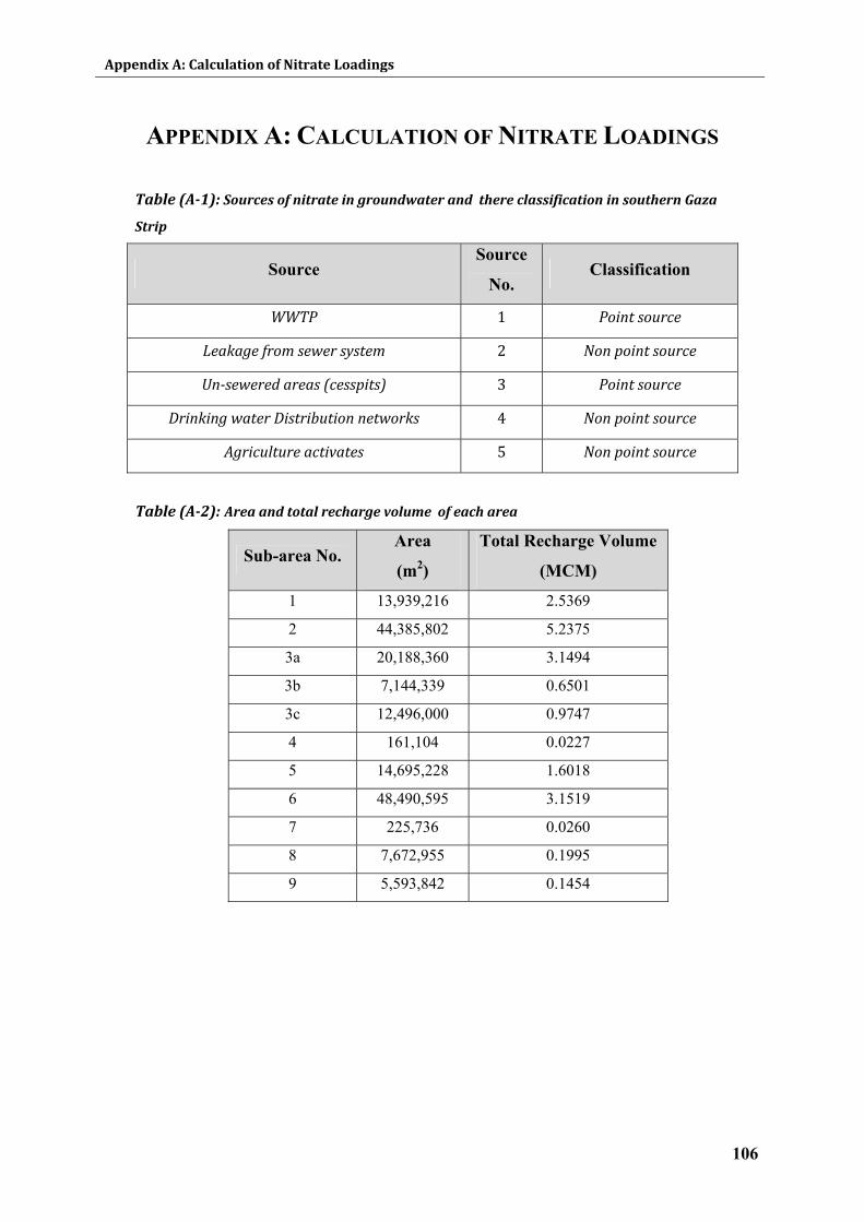
Appendix A: Calculation of Nitrate Loadings
106
APPENDIX A: CALCULATION OF NITRATE LOADINGS
Table (A1): Sources of nitrate in groundwater and there classification in southern Gaza
Strip
Source Source
No. Classification
WWTP 1 Point source
Leakage from sewer system 2 Non point source
Unsewered areas (cesspits) 3 Point source
Drinking water Distribution networks 4 Non point source
Agriculture activates 5 Non point source
Table (A2): Area and total recharge volume of each area
Sub-area No. Area
(m2)
Total Recharge Volume
(MCM)
1 13,939,216 2.5369
2 44,385,802 5.2375
3a 20,188,360 3.1494
3b 7,144,339 0.6501
3c 12,496,000 0.9747
4 161,104 0.0227
5 14,695,228 1.6018
6 48,490,595 3.1519
7 225,736 0.0260
8 7,672,955 0.1995
9 5,593,842 0.1454

Appendix A: Calculation of Nitrate Loadings
107
Figure (A1): Land use map of southern Gaza Strip
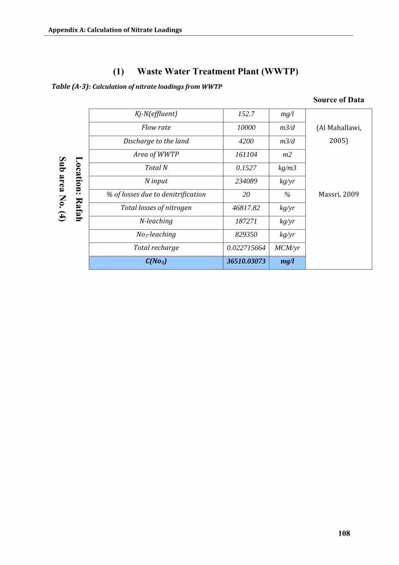
Appendix A: Calculation of Nitrate Loadings
108
(1) Waste Water Treatment Plant (WWTP)
Table (A3): Calculation of nitrate loadings from WWTP
Source of Data
KjN(effluent) 152.7 mg/l
Flow rate 10000 m3/d
Discharge to the land 4200 m3/d
(Al Mahallawi,
2005)
Area of WWTP 161104 m2
Total N 0.1527 kg/m3
N input 234089 kg/yr
% of losses due to denitrification 20 % Massri, 2009
Total losses of nitrogen 46817.82 kg/yr
Nleaching 187271 kg/yr
No3leaching 829350 kg/yr
Total recharge 0.022715664 MCM/yr
Location: R
afah
Sub area No. (4)
C(No3) 36510.03073 mg/l
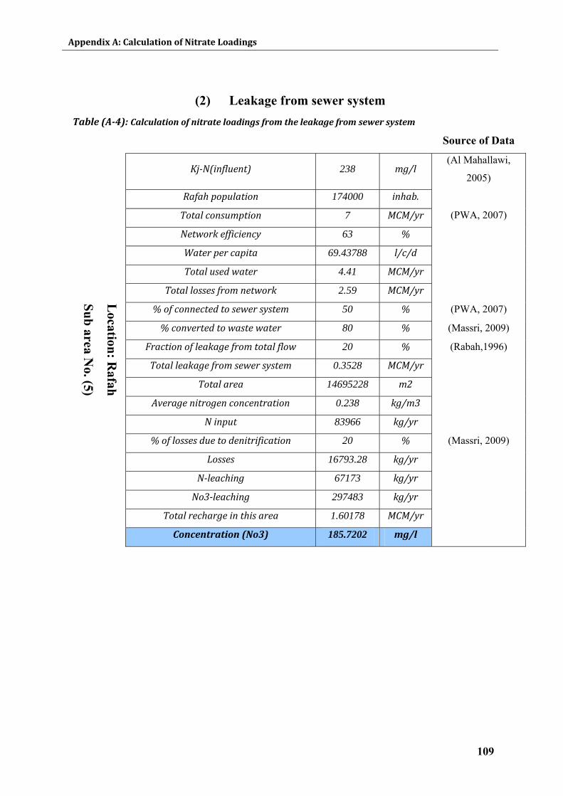
Appendix A: Calculation of Nitrate Loadings
109
(2) Leakage from sewer system
Table (A4): Calculation of nitrate loadings from the leakage from sewer system
Source of Data
KjN(influent) 238 mg/l (Al Mahallawi,
2005)
Rafah population 174000 inhab.
Total consumption 7 MCM/yr
Network efficiency 63 %
(PWA, 2007)
Water per capita 69.43788 l/c/d
Total used water 4.41 MCM/yr
Total losses from network 2.59 MCM/yr
% of connected to sewer system 50 % (PWA, 2007)
% converted to waste water 80 % (Massri, 2009)
Fraction of leakage from total flow 20 % (Rabah,1996)
Total leakage from sewer system 0.3528 MCM/yr
Total area 14695228 m2
Average nitrogen concentration 0.238 kg/m3
N input 83966 kg/yr
% of losses due to denitrification 20 % (Massri, 2009)
Losses 16793.28 kg/yr
Nleaching 67173 kg/yr
No3leaching 297483 kg/yr
Total recharge in this area 1.60178 MCM/yr
Location: R
afah
Sub area No. (5)
Concentration (No3) 185.7202 mg/l
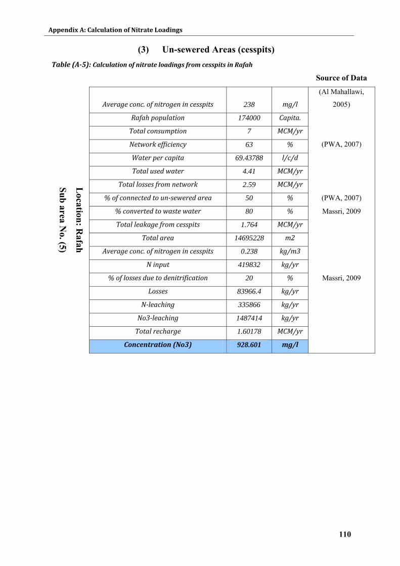
Appendix A: Calculation of Nitrate Loadings
110
(3) Un-sewered Areas (cesspits) Table (A5): Calculation of nitrate loadings from cesspits in Rafah
Source of Data
Average conc. of nitrogen in cesspits 238 mg/l
(Al Mahallawi,
2005)
Rafah population 174000 Capita.
Total consumption 7 MCM/yr
Network efficiency 63 % (PWA, 2007)
Water per capita 69.43788 l/c/d
Total used water 4.41 MCM/yr
Total losses from network 2.59 MCM/yr
% of connected to unsewered area 50 % (PWA, 2007)
% converted to waste water 80 % Massri, 2009
Total leakage from cesspits 1.764 MCM/yr
Total area 14695228 m2
Average conc. of nitrogen in cesspits 0.238 kg/m3
N input 419832 kg/yr
% of losses due to denitrification 20 % Massri, 2009
Losses 83966.4 kg/yr
Nleaching 335866 kg/yr
No3leaching 1487414 kg/yr
Total recharge 1.60178 MCM/yr L
ocation: Rafah
Sub area No. (5)
Concentration (No3) 928.601 mg/l
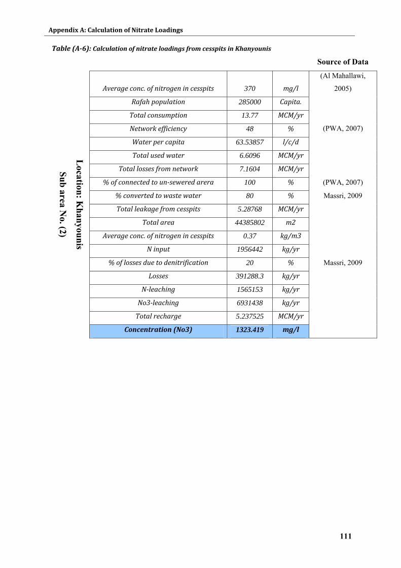
Appendix A: Calculation of Nitrate Loadings
111
Table (A6): Calculation of nitrate loadings from cesspits in Khanyounis
Source of Data
Average conc. of nitrogen in cesspits 370 mg/l
(Al Mahallawi,
2005)
Rafah population 285000 Capita.
Total consumption 13.77 MCM/yr
Network efficiency 48 % (PWA, 2007)
Water per capita 63.53857 l/c/d
Total used water 6.6096 MCM/yr
Total losses from network 7.1604 MCM/yr
% of connected to unsewered arera 100 % (PWA, 2007)
% converted to waste water 80 % Massri, 2009
Total leakage from cesspits 5.28768 MCM/yr
Total area 44385802 m2
Average conc. of nitrogen in cesspits 0.37 kg/m3
N input 1956442 kg/yr
% of losses due to denitrification 20 % Massri, 2009
Losses 391288.3 kg/yr
Nleaching 1565153 kg/yr
No3leaching 6931438 kg/yr
Total recharge 5.237525 MCM/yr L
ocation: Khanyounis
Sub area No. (2)
Concentration (No3) 1323.419 mg/l
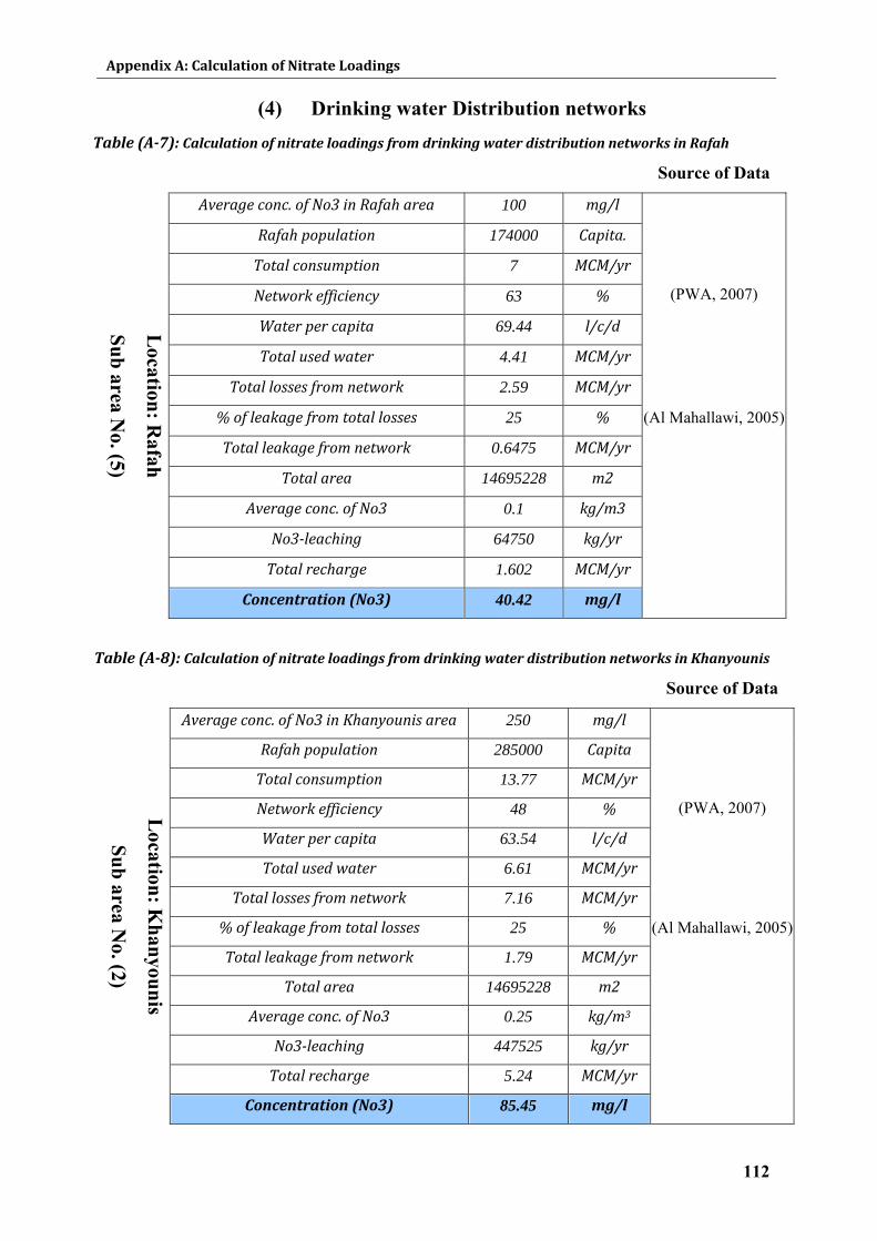
Appendix A: Calculation of Nitrate Loadings
112
(4) Drinking water Distribution networks Table (A7): Calculation of nitrate loadings from drinking water distribution networks in Rafah
Source of Data
Average conc. of No3 in Rafah area 100 mg/l
Rafah population 174000 Capita.
Total consumption 7 MCM/yr
Network efficiency 63 % (PWA, 2007)
Water per capita 69.44 l/c/d
Total used water 4.41 MCM/yr
Total losses from network 2.59 MCM/yr
% of leakage from total losses 25 % (Al Mahallawi, 2005)
Total leakage from network 0.6475 MCM/yr
Total area 14695228 m2
Average conc. of No3 0.1 kg/m3
No3leaching 64750 kg/yr
Total recharge 1.602 MCM/yr
Location: R
afah
Sub area No. (5)
Concentration (No3) 40.42 mg/l
Table (A8): Calculation of nitrate loadings from drinking water distribution networks in Khanyounis
Source of Data
Average conc. of No3 in Khanyounis area 250 mg/l
Rafah population 285000 Capita
Total consumption 13.77 MCM/yr
Network efficiency 48 % (PWA, 2007)
Water per capita 63.54 l/c/d
Total used water 6.61 MCM/yr
Total losses from network 7.16 MCM/yr
% of leakage from total losses 25 % (Al Mahallawi, 2005)
Total leakage from network 1.79 MCM/yr
Total area 14695228 m2
Average conc. of No3 0.25 kg/m3
No3leaching 447525 kg/yr
Total recharge 5.24 MCM/yr
Location: K
hanyounis
Sub area No. (2)
Concentration (No3) 85.45 mg/l
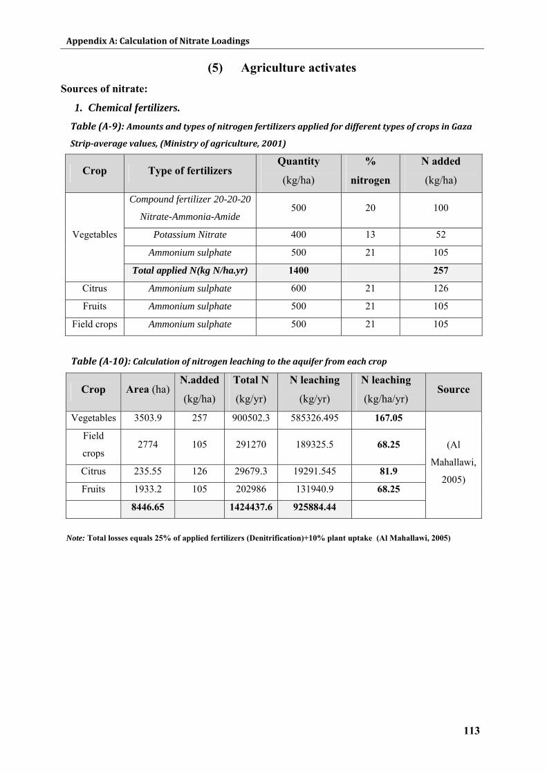
Appendix A: Calculation of Nitrate Loadings
113
(5) Agriculture activates Sources of nitrate:
1. Chemical fertilizers.
Table (A9): Amounts and types of nitrogen fertilizers applied for different types of crops in Gaza
Stripaverage values, (Ministry of agriculture, 2001)
Crop Type of fertilizers Quantity
(kg/ha)
%
nitrogen
N added
(kg/ha)
Compound fertilizer 20-20-20
Nitrate-Ammonia-Amide 500 20 100
Potassium Nitrate 400 13 52
Ammonium sulphate 500 21 105
Vegetables
Total applied N(kg N/ha.yr) 1400 257
Citrus Ammonium sulphate 600 21 126
Fruits Ammonium sulphate 500 21 105
Field crops Ammonium sulphate 500 21 105
Table (A10): Calculation of nitrogen leaching to the aquifer from each crop
Crop Area (ha) N.added
(kg/ha)
Total N
(kg/yr)
N leaching
(kg/yr)
N leaching
(kg/ha/yr) Source
Vegetables 3503.9 257 900502.3 585326.495 167.05
Field
crops 2774 105 291270 189325.5 68.25
Citrus 235.55 126 29679.3 19291.545 81.9
Fruits 1933.2 105 202986 131940.9 68.25
8446.65 1424437.6 925884.44
(Al
Mahallawi,
2005)
Note: Total losses equals 25% of applied fertilizers (Denitrification)+10% plant uptake (Al Mahallawi, 2005)
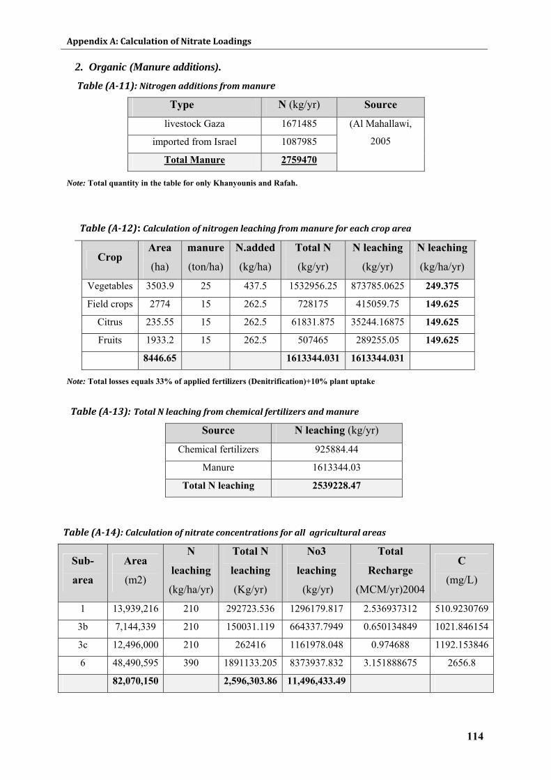
Appendix A: Calculation of Nitrate Loadings
114
2. Organic (Manure additions).
Table (A11): Nitrogen additions from manure
Type N (kg/yr) Source
livestock Gaza 1671485
imported from Israel 1087985
Total Manure 2759470
(Al Mahallawi,
2005
Note: Total quantity in the table for only Khanyounis and Rafah.
Table (A12): Calculation of nitrogen leaching from manure for each crop area
Crop Area
(ha)
manure
(ton/ha)
N.added
(kg/ha)
Total N
(kg/yr)
N leaching
(kg/yr)
N leaching
(kg/ha/yr)
Vegetables 3503.9 25 437.5 1532956.25 873785.0625 249.375
Field crops 2774 15 262.5 728175 415059.75 149.625
Citrus 235.55 15 262.5 61831.875 35244.16875 149.625
Fruits 1933.2 15 262.5 507465 289255.05 149.625
8446.65 1613344.031 1613344.031
Note: Total losses equals 33% of applied fertilizers (Denitrification)+10% plant uptake
Table (A13): Total N leaching from chemical fertilizers and manure
Source N leaching (kg/yr)
Chemical fertilizers 925884.44
Manure 1613344.03
Total N leaching 2539228.47
Table (A14): Calculation of nitrate concentrations for all agricultural areas
Sub-
area
Area
(m2)
N
leaching
(kg/ha/yr)
Total N
leaching
(Kg/yr)
No3
leaching
(kg/yr)
Total
Recharge
(MCM/yr)2004
C
(mg/L)
1 13,939,216 210 292723.536 1296179.817 2.536937312 510.9230769
3b 7,144,339 210 150031.119 664337.7949 0.650134849 1021.846154
3c 12,496,000 210 262416 1161978.048 0.974688 1192.153846
6 48,490,595 390 1891133.205 8373937.832 3.151888675 2656.8
82,070,150 2,596,303.86 11,496,433.49
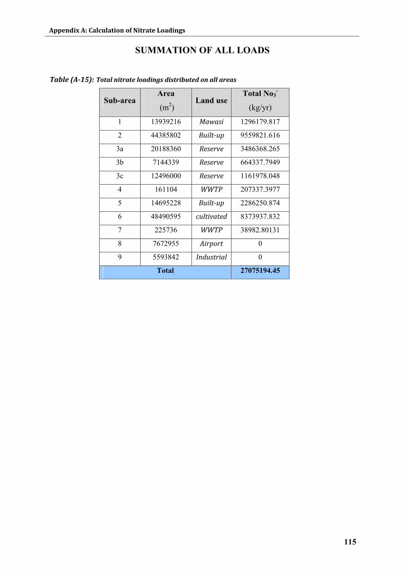
Appendix A: Calculation of Nitrate Loadings
115
SUMMATION OF ALL LOADS
Table (A15): Total nitrate loadings distributed on all areas
Sub-area Area
(m2) Land use
Total No3-
(kg/yr)
1 13939216 Mawasi 1296179.817
2 44385802 Builtup 9559821.616
3a 20188360 Reserve 3486368.265
3b 7144339 Reserve 664337.7949
3c 12496000 Reserve 1161978.048
4 161104 WWTP 207337.3977
5 14695228 Builtup 2286250.874
6 48490595 cultivated 8373937.832
7 225736 WWTP 38982.80131
8 7672955 Airport 0
9 5593842 Industrial 0
Total 27075194.45