waste water
453
-
Upload
beratcansu -
Category
Documents
-
view
218 -
download
3
description
waste water
Transcript of waste water


U.M. Shamsi
GIS Applicationsfor Water, Wastewater,
and Stormwater Systems
Boca Raton London New York Singapore
A CRC title, part of the Taylor & Francis imprint, a member of theTaylor & Francis Group, the academic division of T&F Informa plc.

This book contains information obtained from authentic and highly regarded sources. Reprinted materialis quoted with permission, and sources are indicated. A wide variety of references are listed. Reasonableefforts have been made to publish reliable data and information, but the author and the publisher cannotassume responsibility for the validity of all materials or for the consequences of their use.
Neither this book nor any part may be reproduced or transmitted in any form or by any means, electronicor mechanical, including photocopying, microfilming, and recording, or by any information storage orretrieval system, without prior permission in writing from the publisher.
The consent of CRC Press does not extend to copying for general distribution, for promotion, for creatingnew works, or for resale. Specific permission must be obtained in writing from CRC Press for suchcopying.
Direct all inquiries to CRC Press, 2000 N.W. Corporate Blvd., Boca Raton, Florida 33431.
Trademark Notice:
Product or corporate names may be trademarks or registered trademarks, and areused only for identification and explanation, without intent to infringe.
Visit the CRC Press Web site at www.crcpress.com
© 2005 by CRC Press
No claim to original U.S. Government worksInternational Standard Book Number 0-8493-2097-6
Library of Congress Card Number 2004057108Printed in the United States of America 1 2 3 4 5 6 7 8 9 0
Printed on acid-free paper
Library of Congress Cataloging-in-Publication Data
Shamsi, U. M. (Uzair M.)GIS applications for water, wastewater, and stormwater systems / U.M. Shamsi. p. cm.Includes bibliographical references and index.ISBN 0-8493-2097-6 (alk. paper) 1. Water—Distribution. 2. Sewage disposal. 3. Runoff—Management. 4. Geographic
information systems. I. Title.
TD482.S53 2005 628.1—dc22 2004057108
2097 disclaimer.fm Page 2 Wednesday, October 20, 2004 7:08 AM

Dedication
Dedicated to my beloved wife, Roshi, and my children, Maria, Adam, and Harris


Preface
To fully appreciate the benefits of GIS applications consider the followinghypothetical scenario. On March 10, 2004, following a heavy storm event, a sewercustomer calls the Sewer Authority of the City of Cleanwater to report minorbasement flooding without any property damage. An Authority operator immediatelystarts the GIS and enters the customer address. GIS zooms to the resident propertyand shows all the sewers and manholes in the area. The operator queries the inspec-tion data for a sewer segment adjacent to the customer property and finds that amini movie of the closed-circuit television (CCTV) inspection dated July 10, 1998,is available. The operator plays the movie and sees light root growth in the segment.A query of the maintenance history for that segment indicates that it has not beencleaned since April 5, 1997. This information indicates that the roots were nevercleaned and have probably grown to “heavy” status. The operator highlights thesewer segment, launches the work order module, and completes a work order formfor CCTV inspection and root removal, if necessary. The export button saves thework order form and a map of the property and adjacent sewers in a PDF file. Theoperator immediately sends the PDF file by e-mail to the Authority’s sewer cleaningcontractor. The entire session from the time the customer called the Authority officetook about 30 min. The operator does not forget to call the customer to tell him thata work order has been issued to study the problem. This book presents the methodsand examples required to develop applications such as this.
The days of the slide rule are long gone. Word processors are no longer consid-ered cutting-edge technology. We are living in an information age that requires usto be more than visionaries who can sketch an efficient infrastructure plan. Thistech-heavy society expects us to be excellent communicators who can keep all thestakeholders — the public, the regulators, or the clients — “informed.” New infor-mation and decision support systems have been developed to help us to be goodcommunicators. GIS is one such tool that helps us to communicate geographic orspatial information. The real strength of GIS is its ability to integrate information.GIS helps decision makers by pulling together crucial bits and pieces of informationas a whole and showing them the “big picture.” In the past 10 years, the number ofGIS users has increased substantially. Many of us are using GIS applications on theInternet and on wireless devices without even knowing that we are using a GIS.Experts believe that in the near future, most water, wastewater, and stormwatersystem professionals will be using the GIS in the same way they are now using aword processor or spreadsheet. Except for the computer itself, no technology hasso revolutionized the water industry. The time has come for all the professionalsinvolved in the planning, design, construction, and operation of water, wastewater,and stormwater systems to enter one of the most promising and exciting technologiesof the millennium in their profession — GIS applications.
According to some estimates, more than 80% of all the information used by water andsewer utilities is geographically referenced.

This book was inspired from a continuing education course that the author hasbeen teaching since 1998 for the American Society of Civil Engineers (ASCE).Entitled ‘‘GIS Applications in Water, Wastewater and Stormwater Systems,” theseminar course has been attended by hundreds of water, wastewater, and stormwaterprofessionals in major cities of the United States. Many models, software, examples,and case studies described in the book (especially those from Pennsylvania) arebased on the GIS projects worked on or managed by the author himself.
This is my second GIS book for water, wastewater, and stormwater systems. Thefirst book, GIS Tools for Water, Wastewater, and Stormwater Systems, published byAmerican Society of Civil Engineers (ASCE) Press in 2002, was a huge success.The first printing was sold out, and the book achieved ASCE Press’s best-sellerstatus within months of publication. Whereas the first book focused on GIS basicsand software and data tools to develop GIS applications, this second book focuseson the practical applications of those tools. Despite the similarity of the titles, bothbooks cover different topics and can be read independent of each other.
STYLE OF THE BOOK
This book has been written using the recommendations of the AccreditationBoard for Engineering and Technology (ABET) of the U.S. and the American Societyof Civil Engineers’ (ASCE) Excellence in Civil Engineering Education (ExCEEd)program. Both of these organizations recommend performance- (or outcome-) basedlearning in which the learning objectives of each lecture (or chapter) are clearlystated up front, and the learning is measured in terms of achieving these learningobjectives. Each chapter of this book accordingly starts with learning objectives forthat chapter and ends with a chapter summary and questions. Most technical booksare written using the natural human teaching style called deductive, in which prin-ciples are presented before the applications. In this book, an attempt has been madeto organize the material in the natural human learning style called inductive, in whichexamples are presented before the principles. For example, in most chapters, casestudies are presented before the procedures are explained. The book has numerousmaps and illustrations that should cater well to the learning styles of “visual learners”— GIS, after all is regarded as a visual language.
The primary learning objective of this book is to document GIS applications for water,wastewater, and stormwater systems. This book will show you how to use GIS to make taskseasier to do and increase productivity, and hence, save time and money in your business.
ORGANIZATION OF THE BOOK
There are 17 chapters in this book, organized as follows:
• Chapter 1, GIS Applications: Describes why GIS applications are important andhow they are created

• Chapter 2, Needs Analysis: Explains how to avoid potential pitfalls of GIS imple-mentation by starting with a needs analysis study
The next five chapters describe four GIS-related technologies that are verybeneficial in developing GIS applications:
• Chapter 3, Remote Sensing Applications: Shows how to use satellite imagery inGIS applications
• Chapter 4, DEM Applications: Describes the methods of incorporating digitalelevation model (DEM) data
• Chapter 5, GPS Applications: Discusses how to benefit from global positioningsystem (GPS) technology
• Chapter 6, Internet Applications: Explains the applications of Internet technologyin serving GIS maps on the Internet
• Chapter 7, Mobile GIS: Provides information on using GIS in the field for inspec-tion and maintenance work
The GIS applications that are of particular importance to water industry profes-sionals are: Mapping, Monitoring, Modeling, and Maintenance. These four Ms definesome of the most important activities for efficient management of water, wastewater,and stormwater systems, and are referred to as the “4M applications” in this book.The next ten chapters focus on these four Ms.
• Chapter 8, Mapping: Describes how to create the first M of the 4M applications• Chapter 9, Mapping Applications: Describes examples of the first M of the 4M
applications• Chapter 10, Monitoring Applications: Describes the applications of the second M
of the 4M applications• Chapter 11, Modeling Applications: Describes the applications of the third M of
the 4M applications• Chapter 12, Water Models: Describes examples of the third M of the 4M appli-
cations for modeling water distribution systems• Chapter 13, Sewer Models: Describes examples of the third M of the 4M appli-
cations for modeling sewage collection systems• Chapter 14, AM/FM/GIS Applications: Describes automated mapping/facilities
management/geographic information system (AM/FM/GIS) software tools forimplementing the fourth M of the 4M applications
• Chapter 15, Maintenance Applications: Describes the applications of the fourthM of the 4M applications
• Chapter 16, Security Planning and Vulnerability Assessment: Discusses GIS appli-cations for protecting water and wastewater systems against potential terroristattacks
• Chapter 17, Applications Sampler: Presents a collection of recent case studiesfrom around the world


Acknowledgments
Case studies presented in Chapter 17, Applications Sampler, were written spe-cially for publication in this book by 18 GIS and water industry experts from 6countries (Belgium, Bulgaria, Czech Republic, Denmark, Spain and the United States)in response to my call for case studies distributed to various Internet discussionforums. I thank these case study authors for their contributions to this book:
• Bart Reynaert, Rene Horemans, and Patrick Vercruyssen of Pidpa, Belgium• Carl W. Chen and Curtis Loeb of Systech Engineering, Inc., San Ramon, California• Dean Trammel, Tucson Water, Tucson, Arizona• Ed Bradford, Roger Watson, Eric Mann, Jenny Konwinski of Metropolitan
Sewerage District of Buncombe County, North Carolina• Eric Fontenot of DHI, Inc., Hørsholm, Denmark• Milan Suchanek and Tomas Metelka of Sofiyska Voda A.D., Sofia, Bulgaria• Peter Ingeduld, Zdenek Svitak, and Josef Drbohlav of Praûská vodohospodáská
spolenost a.s. (Prague stockholding company), Prague, Czech Republic• Hugo Bartolin and Fernando Martinez of Polytechnic University of Valencia,
Spain
I also thank the following organizations and companies for providing infor-mation for this book: American Society of Civil Engineers, American Water WorksAssociation, Azteca Systems, CE Magazine, CH2M Hill, Chester Engineers, Compu-tational Hydraulics International, Danish Hydraulic Institute (DHI), EnvironmentalSystems Research Institute, Geospatial Solutions Magazine, GEOWorld Magazine,Haestad Methods, Hansen Information Technology, Journal of the American WaterResources Association, Journal of the American Water Works Association, MWH Soft,Professional Surveyor Magazine, USFilter, Water Environment Federation, and WaterEnvironment & Technology Magazine. Some information presented in this book isbased on my collection of papers and articles published in peer-reviewed journals,trade magazines, conference proceedings, and the Internet. The authors and organiza-tions of these publications are too numerous to be thanked individually, so I thankthem all collectively without mentioning their names. Their names are, of course,included in the Reference section.
Finally, I would like to thank you for buying the book. I hope you will find thebook useful in maximizing the use of GIS in your organization to make things easierto do, increase productivity, and save time and money.


About the Author
Uzair (Sam) M. Shamsi, Ph.D., P.E., DEE is director ofthe GIS and Information Management Technology divisionof Chester Engineers, Pittsburgh, Pennsylvania, and anadjunct assistant professor at the University of Pittsburgh,where he teaches GIS and hydrology courses. His areas ofspecialization include GIS applications and hydrologic andhydraulic (H&H) modeling. He has been continuingeducation instructor for the American Society of CivilEngineers (ASCE) and an Environmental Systems ResearchInstitute (ESRI)-authorized ArcView® GIS instructor since1998. He has taught GIS courses to more than 500professionals throughout the United States, including a course on “GIS Applicationsin Water, Wastewater, and Stormwater Systems” for ASCE. Sam earned his Ph.D.in civil engineering from the University of Pittsburgh in 1988. He has 20 years ofGIS and water and wastewater engineering experience in teaching, research, andconsulting. His accomplishments include more than 120 projects and over 100lectures and publications, mostly in GIS applications. His previous book, GIS Toolsfor Water, Wastewater, and Stormwater Systems, was an ASCE Press best seller. Heis the recipient of the ASCE’s Excellence in Civil Engineering Education (EXCEED)training and is a licensed professional engineer in Pennsylvania, Ohio, and WestVirginia. In addition to ASCE, he is a member of the American Water ResourcesAssociation, the Water Environment Foundation, and the American Water WorksAssociation.
E-mail: [email protected] site: www.GISApplications.com


GIS is an instrument for implementing geographic thinking.
Jack Dangermond (1998)
Iron rusts from disuse; water loses its purity from stagnation and in cold weatherbecomes frozen; even so does inaction sap the vigors of the mind.
Leonardo da Vinci (1452–1519)
Life is like a sewer
…what you get out of it depends on what you put into it.
Tom Lehrer (1928–)
Times of general calamity and confusion create great minds. The purest ore isproduced from the hottest furnace, and the brightest thunderbolt is elicited from thedarkest storms.
Charles Caleb Colton (1780–1832)


Contents
Chapter 1 GIS Applications Learning Objective ....................................................................................................2Major Topics ..............................................................................................................2List of Chapter Acronyms .........................................................................................2Introduction................................................................................................................2What Are GIS Applications? ....................................................................................3History of GIS Applications .....................................................................................44M Applications .......................................................................................................6Advantages and Disadvantages of GIS Applications .............................................. 6
Advantages .......................................................................................................7GIS Applications Save Time and Money.............................................7GIS Applications Are Critical to Sustaining GIS Departments...........7GIS Applications Provide the Power of Integration............................8GIS Applications Offer a Decision Support Framework.....................8GIS Applications Provide Effective Communication Tools.................9GIS Applications Are Numerous..........................................................9
Disadvantages.................................................................................................12Success Stories ........................................................................................................13
San Diego.......................................................................................................13Boston.............................................................................................................13Cincinnati .......................................................................................................13Knoxville ........................................................................................................14Dover ..............................................................................................................14Charlotte .........................................................................................................14Albany County ...............................................................................................14GIS Applications Around the World..............................................................15
Evolving GIS Applications and Trends...................................................................15Future Applications and Trends ..............................................................................16GIS Application Development Procedure ...............................................................19Application Programming .......................................................................................20
GIS-Based Approach......................................................................................20GIS Customization.............................................................................20Scripting .............................................................................................20Extensions ..........................................................................................21External Programs..............................................................................23
Application-Based Approach .........................................................................24Useful Web Sites .....................................................................................................24Chapter Summary ....................................................................................................24Chapter Questions....................................................................................................25
Chapter 2 Needs AnalysisLearning Objective ..................................................................................................28Major Topics ............................................................................................................28

List of Chapter Acronyms .......................................................................................28Ocean County’s Strategic Plan................................................................................28Introduction..............................................................................................................28Needs Analysis Steps...............................................................................................29
Step 1. Stakeholder Identification..................................................................30Step 2. Stakeholder Communication .............................................................30
Introductory Seminar .........................................................................31Work Sessions and Focus Groups .....................................................31Interviews ...........................................................................................31
Step 3. Resource Inventory............................................................................32Step 4. Need Priorities ...................................................................................33Step 5. System Design ...................................................................................33
Data Conversion (Mapping)...............................................................33Database .............................................................................................34Software Selection .............................................................................36Hardware Selection ............................................................................37User Interface .....................................................................................38
Step 6. Pilot Project .......................................................................................40Step 7. Implementation Plan..........................................................................41Step 8. Final Presentation ..............................................................................43
Needs Analysis Examples .......................................................................................43Pittsburgh, Pennsylvania ................................................................................43Borough of Ramsey, New Jersey...................................................................44The City of Bloomington, Indiana ................................................................45San Mateo County, California .......................................................................45
Chapter Summary ....................................................................................................45Chapter Questions....................................................................................................46
Chapter 3 Remote Sensing Applications Learning Objective ..................................................................................................48Major Topics ............................................................................................................48List of Chapter Acronyms .......................................................................................48Albany County’s Remote Sensing Application.......................................................48Introduction..............................................................................................................49Remote Sensing Applications..................................................................................51Remote Sensing Satellites .......................................................................................52Spatial Resolution....................................................................................................53
Low-Resolution Satellite Data.......................................................................53Medium-Resolution Satellite Data.................................................................54High-Resolution Satellite Data ......................................................................56
High-Resolution Satellites .................................................................56High-Resolution Imagery Applications .............................................58
Data Sources ..................................................................................................59Digital Orthophotos .................................................................................................59
USGS Digital Orthophotos ............................................................................60Case Study: Draping DOQQ Imagery on DEM Data.......................62

Examples of Remote Sensing Applications ............................................................62LULC Classification ......................................................................................62Soil Moisture Mapping ..................................................................................65Estimating Meteorological Data ....................................................................66
Geographic Imaging and Image Processing Software............................................66ERDAS Software Products ............................................................................66
ERDAS Software Application Example ............................................68ArcView Image Analysis Extension ..............................................................69MrSID.............................................................................................................69PCI Geomatics ...............................................................................................70Blue Marble Geographics ..............................................................................71
Future Directions .....................................................................................................72Useful Web Sites .....................................................................................................73Chapter Summary ....................................................................................................73Chapter Questions....................................................................................................73
Chapter 4 DEM ApplicationsLearning Objective ..................................................................................................76Major Topics ............................................................................................................76List of Chapter Acronyms .......................................................................................76Hydrologic Modeling of the Buffalo Bayou Using GIS and DEM Data ..............76DEM Basics .............................................................................................................77DEM Applications ...................................................................................................79
Three-Dimensional (3D) Visualization..........................................................79DEM Resolution and Accuracy...............................................................................80USGS DEMs............................................................................................................81
USGS DEM Formats .....................................................................................82National Elevation Dataset (NED) ....................................................83
DEM Data Availability ............................................................................................83DEM Data Creation from Remote Sensing ............................................................84
Image Processing Method..............................................................................84Data Collection Method.................................................................................84LIDAR............................................................................................................85IFSAR.............................................................................................................85
DEM Analysis..........................................................................................................86Cell Threshold for Defining Streams.............................................................86The D-8 Model...............................................................................................86DEM Sinks.....................................................................................................87Stream Burning ..............................................................................................88DEM Aggregation ..........................................................................................88Slope Calculations..........................................................................................88
Software Tools .........................................................................................................88Spatial Analyst and Hydro Extension............................................................90ARC GRID Extension ...................................................................................93IDRISI ............................................................................................................94TOPAZ ...........................................................................................................95

Case Studies and Examples.....................................................................................95Watershed Delineation ...................................................................................95Sewershed Delineation.................................................................................101Water Distribution System Modeling ..........................................................103
WaterCAD Example.........................................................................104Useful Web Sites ...................................................................................................105Chapter Summary ..................................................................................................105Chapter Questions..................................................................................................106
Chapter 5 GPS ApplicationsLearning Objective ................................................................................................108Major Topics ..........................................................................................................108List of Chapter Acronyms .....................................................................................108Stream Mapping in Iowa .......................................................................................108GPS Basics ............................................................................................................109GPS Applications in the Water Industry ...............................................................110
Surveying......................................................................................................111Fleet Management........................................................................................111
GPS Applications in GIS.......................................................................................111GPS Survey Steps..................................................................................................112GPS Equipment .....................................................................................................113
Recreational GPS Equipment ......................................................................113Basic GPS Equipment..................................................................................114Advanced GPS Equipment ..........................................................................115
Survey Grade GPS Equipment..............................................................................116Useful Web Sites ...................................................................................................117Chapter Summary ..................................................................................................117Chapter Questions..................................................................................................118
Chapter 6 Internet ApplicationsLearning Objective ................................................................................................120Major Topics ..........................................................................................................120List of Chapter Acronyms .....................................................................................120Dublin’s Web Map.................................................................................................120Internet GIS ...........................................................................................................122
Internet Security...........................................................................................123Internet GIS Software............................................................................................124Internet GIS Applications ......................................................................................124
Data Integration............................................................................................124Project Management ....................................................................................1243D Visualization Applications .....................................................................126
Case Studies...........................................................................................................126Tacoma’s Intranet and Mobile GIS .............................................................126Montana’s Watershed Data Information Management System...................127
Useful Web Sites ...................................................................................................128

Chapter Summary ..................................................................................................128Chapter Questions..................................................................................................128
Chapter 7 Mobile GISLearning Objective ................................................................................................130Major Topics ..........................................................................................................130List of Chapter Acronyms .....................................................................................130Mobile GIS Basics.................................................................................................130Mobile GIS Applications.......................................................................................131Wireless Internet Technology ................................................................................133GPS Integration .....................................................................................................133Useful Web Sites ...................................................................................................134Chapter Summary ..................................................................................................135Chapter Questions..................................................................................................135
Chapter 8 MappingLearning Objective ................................................................................................138Major Topics ..........................................................................................................138List of Chapter Acronyms .....................................................................................138Los Angeles County’s Sewer Mapping Program..................................................138Mapping Basics .....................................................................................................139
Map Types ....................................................................................................139Topology.......................................................................................................139Map Projections and Coordinate Systems...................................................140Map Scale.....................................................................................................140Data Quality .................................................................................................140Data Errors ...................................................................................................141Map Accuracy ..............................................................................................141
Map Types..............................................................................................................142Base Map......................................................................................................142
Digital Orthophotos..........................................................................143Planimetric Maps .............................................................................143Small-Scale Maps ............................................................................144
Advantages of GIS Maps ......................................................................................145GIS Mapping Steps ...............................................................................................147
Needs Analysis .............................................................................................147Data Collection ............................................................................................148Data Conversion...........................................................................................148
Capturing Attributes .........................................................................148Capturing Graphics ..........................................................................149
Digitization........................................................................149Scanning............................................................................150Data Conversion Software................................................150
Data Processing............................................................................................153Data Preparation...............................................................................153Topological Structuring....................................................................153

Data Management ............................................................................154Quality Control ................................................................................155Map Production................................................................................155
Case Studies...........................................................................................................156Borough of Ramsey, New Jersey.................................................................156City of Lake Elsinore, California ................................................................158Allegheny County, Pennsylvania .................................................................159
Useful Web Sites ...................................................................................................159Chapter Summary ..................................................................................................160Chapter Questions..................................................................................................160
Chapter 9 Mapping ApplicationsLearning Objective ................................................................................................162Major Topics ..........................................................................................................162List of Chapter Acronyms .....................................................................................162Customer Service Application in Gurnee .............................................................162Common Mapping Functions................................................................................164
Thematic Mapping .......................................................................................164Spatial Analysis............................................................................................164Buffers ..........................................................................................................164Hyperlinks ....................................................................................................167
Water System Mapping Applications....................................................................167MWRA Water System Mapping Project .....................................................167Service Shutoff Application.........................................................................167Generating Meter-Reading Routes ..............................................................169Map Maintenance Application.....................................................................169
Wastewater System Mapping Applications...........................................................169Public Participation with 3D GIS................................................................169Mapping the Service Laterals ......................................................................170
Stormwater System Mapping Applications...........................................................173Stormwater Permits......................................................................................173
Chapter Summary ..................................................................................................175Chapter Questions..................................................................................................175
Chapter 10 Monitoring ApplicationsLearning Objective ................................................................................................178Major Topics ..........................................................................................................178List of Chapter Acronyms .....................................................................................178Monitoring Real Time Rainfall and Stream-Flow Data in Aurora.......................178Monitoring Basics..................................................................................................179Remotely Sensed Rainfall Data ............................................................................179
Satellite Rainfall Data ..................................................................................180Radar Rainfall Data .....................................................................................181NEXRAD Rainfall Data ..............................................................................181
NEXRAD Level III Data .................................................................181Estimating Rainfall Using GIS ....................................................................183

Radar Rainfall Application: Virtual Rain-Gauge Case Study.....................184Flow-Monitoring Applications ..............................................................................187
SCADA Integration..................................................................................... 187NPDES-Permit Reporting Applications ............................................................... 188Monitoring via Internet .........................................................................................189Monitoring the Infrastructure ................................................................................190Useful Web Sites ...................................................................................................190Chapter Summary ..................................................................................................191Chapter Questions..................................................................................................191
Chapter 11 Modeling ApplicationsLearning Objectives...............................................................................................194Major Topics ..........................................................................................................194List of Chapter Acronyms .....................................................................................194Temporal-Spatial Modeling in Westchester County .............................................194H&H Modeling......................................................................................................195Application Methods .............................................................................................196Interchange Method...............................................................................................197
Subbasin Parameter Estimation ...................................................................198Runoff Curve Number Estimation...............................................................199Water Quality Modeling Data Estimation ...................................................200Demographic Data Estimation.....................................................................202Land-Use Data Estimation...........................................................................204
Interface Method....................................................................................................205HEC-GEO Interface .....................................................................................207HEC-GeoHMS .............................................................................................207HEC-GeoRAS ..............................................................................................207Watershed Modeling System .......................................................................208GISHydro Modules ......................................................................................208
GISHydro Prepro .............................................................................209GISHydro Runoff.............................................................................210
ArcInfo Interface with HEC Programs........................................................210Intermediate Data Management Programs ..................................................211Interface Method Case Study ......................................................................212
Integration Method ................................................................................................212EPA’s BASINS Program ..............................................................................213
BASINS Examples...........................................................................217MIKE BASIN...............................................................................................218Geo-STORM Integration .............................................................................219ARC/HEC-2 Integration ..............................................................................219Integration Method Case Study ...................................................................220
Which Linkage Method to Use? ...........................................................................221Useful Web Sites ...................................................................................................222Chapter Summary ..................................................................................................222Chapter Questions..................................................................................................223
Chapter 12 Water ModelsLearning Objective ................................................................................................226Major Topics ..........................................................................................................226List of Chapter Acronyms .....................................................................................226City of Germantown’s Water Model .....................................................................226GIS Applications for Water Distribution Systems ................................................227Development of Hydraulic Models .......................................................................229Software Examples ................................................................................................231
EPANET.......................................................................................................231H2ONET™ and H2OMAP™ ..........................................................................232
Demand Allocator ............................................................................235Skeletonizer ......................................................................................235Tracer................................................................................................235
WaterCAD™ and WaterGEMS™ ..................................................................235MIKE NET™.................................................................................................236Other Programs ............................................................................................237
EPANET and ArcView Integration in Harrisburg.................................................237Mapping the Model Output Results ............................................................242
Network Skeletonization .......................................................................................243Estimation of Node Demands ...............................................................................249
Demand-Estimation Case Studies................................................................252Newport News, Virginia...................................................................252Round Rock, Texas ..........................................................................252Lower Colorado River Authority, Texas..........................................253
Estimation of Node Elevations..............................................................................253Pressure Zone Trace..............................................................................................255Chapter Summary ..................................................................................................255Chapter Questions..................................................................................................255
Chapter 13 Sewer ModelsLearning Objectives...............................................................................................258Major Topics...........................................................................................................258List of Chapter Acronyms .....................................................................................258MapInfo™ and SWMM Interchange..................................................................... 258GIS Applications for Sewer Systems ................................................................... 259Sewer System Modeling Integration .................................................................... 260Software Examples ............................................................................................... 261SWMM ................................................................................................................. 261Useful SWMM Web Sites .................................................................................... 264
SWMM Graphical User Interface .............................................................. 264XP-SWMM and XP-GIS ................................................................ 266
GIS Data for SWMM ................................................................................. 267Estimating Green-Ampt Parameters Using STATSGO/SSURGO GIS Files ...................................................................................... 267
GIS Applications for SWMM .............................................................................. 270

AVSWMM................................................................................................... 270AVSWMM RUNOFF Extension .................................................... 271AVSWMM EXTRAN Extension.................................................... 274
Task 1: Create EXTRAN input file .................................... 274Task 2: Create SWMM EXTRAN output layers in ArcViewGIS .................................................................... 277
SWMMTools ............................................................................................... 278AGSWMM .................................................................................................. 280PCSWMM GIS™.......................................................................................... 281SWMM and BASINS ................................................................................. 282SWMMDUET ............................................................................................. 283AVsand™...................................................................................................... 284
Other Sewer Models ............................................................................................. 284DHI Models................................................................................................. 284
MOUSE™ ........................................................................................ 284MIKE SWMM ™ ............................................................................ 285MOUSE GIS™................................................................................. 285MOUSE GM ™ ................................................................................ 286
InfoWorks™ ................................................................................................. 287SewerCAD™ and StormCAD™ .................................................................. 289
Sewer Modeling Case Studies.............................................................................. 289XP-SWMM and ArcInfo Application for CSO Modeling ......................... 289AM/FM/GIS and SWMM Integration........................................................ 290SWMM and ArcInfo™ Interface................................................................. 290Hydra™ and ArcInfo™ Interface.................................................................. 291
Useful Web Sites .................................................................................................. 291Chapter Summary ................................................................................................. 291Chapter Questions................................................................................................. 292
Chapter 14 AM/FM/GIS ApplicationsLearning Objective ................................................................................................294Major Topics ..........................................................................................................294List of Chapter Acronyms .....................................................................................294Hampton’s Wastewater Maintenance Management ..............................................294Infrastructure Problem...........................................................................................295AM/FM/GIS Basics ...............................................................................................297
Automated Mapping (AM) ..........................................................................298Facilities Management (FM) .......................................................................300Automated Mapping (AM)/Facilities Management (FM)...........................300AM/FM/GIS Systems ..................................................................................300
AM/FM/GIS Software ...........................................................................................300ArcFM ..........................................................................................................302Cityworks .....................................................................................................304
Chapter Summary ..................................................................................................305Chapter Questions..................................................................................................305

Chapter 15 Maintenance ApplicationsLearning Objective ................................................................................................308Major Topics ..........................................................................................................308List of Chapter Acronyms .....................................................................................308Buncombe County’s Sewer System Inspection and Maintenance .......................309Asset Management ................................................................................................310GASB 34 Applications ..........................................................................................312Wet Weather Overflow Management Applications ...............................................312
AutoCAD Map GIS Application for CMOM .............................................313CCTV Inspection of Sewers..................................................................................314
Convert Existing Video Tapes to Digital Files ............................................315Digitize Existing VHS Tapes .......................................................................316
WinCan.............................................................................................317Retrofit Tape Systems with Digital Systems ...............................................317Record Directly in Digital Format...............................................................319Linking Digital Movies to GIS....................................................................319
Video Mapping ......................................................................................................321Thematic Mapping of Inspection Data .................................................................322Work Order Management ..................................................................................... 325Water Main Isolation Trace...................................................................................327Case Studies...........................................................................................................328
Isolation Trace Case Studies........................................................................328Sewer System Inspections in Washington County ......................................328Sewer Rehabilitation in Baldwin ................................................................330
Useful Web Sites ...................................................................................................333Chapter Summary ..................................................................................................333Chapter Questions..................................................................................................333
Chapter 16 Security Planning and Vulnerability AssessmentLearning Objective ................................................................................................336Major Topics ..........................................................................................................336List of Chapter Acronyms .....................................................................................336GIS Applications in Planning................................................................................336Security Planning...................................................................................................337
Vulnerability of Water Systems ...................................................................338Vulnerability of Sewer Systems...................................................................338
GIS Applications in Vulnerability Assessment .....................................................338Security Modeling Software .................................................................................340
H2OMAP™ Protector................................................................................... 340WaterSAFE™ ................................................................................................340VSAT™ .........................................................................................................342
Security Planning Data Issues...............................................................................342Useful Web Sites ...................................................................................................343Chapter Summary ..................................................................................................343Chapter Questions................................................................................................. 343

Chapter 17 Applications SamplerLearning Objective ................................................................................................346Major Topics ..........................................................................................................346List of Chapter Acronyms .....................................................................................346Drainage Area Planning in Sofia...........................................................................346Pipe Rating Program in Buncombe County .........................................................347Water System Modeling in Tucson .......................................................................352Water System Modeling in the City of Truth or Consequences..........................353
Background ..................................................................................................355Building the MIKE NET Model from Various Data Sources.....................355
ArcGIS and ArcFM Integration in Belgium .........................................................356Water System Master Planning in Prague ............................................................358Water Quality Management in Mecklenburg County...........................................360Water Master Planning in Sueca, Spain................................................................362Chapter Summary ..................................................................................................364Chapter Questions..................................................................................................364
Appendix A Acronyms........................................................................................365Appendix B Conversion Factors..........................................................................371References .............................................................................................................373Index......................................................................................................................389


1
CHAPTER 1
GIS Applications
Geographic Information System (GIS) is one of the most promisingand exciting technology of the decade in our profession. This bookwill show you that with GIS the possibilities to manage your water,wastewater, and stormwater systems are almost endless.
GIS applications can take you from work frustration to job satisfaction.

2 GIS APPLICATIONS FOR WATER, WASTEWATER, AND STORMWATER SYSTEMS
LEARNING OBJECTIVE
The learning objective of this chapter is to understand the importance and scope ofgeographic information system (GIS) applications for water, wastewater, and storm-water systems.
MAJOR TOPICS
• Definition of GIS applications• History of GIS applications• Advantages and disadvantages of GIS applications• Evolving and future GIS applications and trends• Methods of developing GIS applications
LIST OF CHAPTER ACRONYMS*
CAD Computer-Aided Drafting/Computer-Aided DesignESRI Environmental Systems Research InstituteGIS Geographic Information SystemsGPS Global Positioning SystemGUI Graphical User InterfaceH&H Hydrologic and HydraulicLBS Location-Based ServicesPC Personal ComputerPDA Personal Digital Assistant
GIS Project Nominated for OCEA Award
American Society of Civil Engineers (ASCE) awards Outstanding Civil EngineeringAchievement (OCEA) awards to projects based on their contribution to the well-being ofpeople and communities; resourcefulness in planning and solving design challenges;pioneering in use of materials and methods; innovations in construction; impact on physicalenvironment; and beneficial effects including aesthetic value. The Adam County (Illinois)2002 GIS Pilot Project was a nominee for the 1997 awards. This project was a 10-year,multiparticipant (Adams County, City of Quincy, Two Rivers Regional Planning Council,and a number of state and local agencies) project to develop an accurate, updated GISdesigned to create a more efficient local government.
INTRODUCTION
The water industry** business is growing throughout the world. For example,the U.S. market for water quality systems and services had a total value of $103billion in 2000. The two largest components of this business are the $31-billion
* Each chapter of this book begins with a list of frequently used acronyms in the chapter. Appendix Aprovides a complete list of acronyms used in the book.** In this book, the term water industry refers to water, wastewater, and stormwater systems.

GIS APPLICATIONS 3
public wastewater treatment market and the $29-billion water supply market (Farkasand Berkowitz, 2001).
One of the biggest challenges in the big cities with aging water, wastewater,and stormwater infrastructures is managing information about maintenance ofexisting infrastructure and construction of new infrastructure. Many utilities tackleinfrastructure problems on a react-to-crisis basis that, despite its conventionalwisdom, may not be the best strategy. Making informed infrastructure improve-ment decisions requires a large amount of diverse information on a continuingbasis. If information is the key to fixing infrastructure problems, the first step of anyinfrastructure improvement project should be the development of an informationsystem.
An information system is a framework that provides answers to questions, froma data resource. A GIS is a special type of information system in which the datasource is a database of spatially distributed features and procedures to collect, store,retrieve, analyze, and display geographic data (Shamsi, 2002).
More than 80% of all the information used by water and wastewater utilities isgeographically referenced.
In other words, a key element of the information used by utilities is its locationrelative to other geographic features and objects. GIS technology that offers thecombined power of both geography and information systems is an ideal solution foreffective management of water industry infrastructure. Geotechnology and geospa-tial technology are alias names of GIS technology.
The days of the slide rule are long gone. Word processors are no longer consid-ered cutting-edge technology. We are living in the information age, which requiresus to be more than visionaries who can sketch an efficient infrastructure plan. Today’stech-savvy society expects us to be excellent communicators who can keep all thestakeholders — the public, the regulators, or the clients — “informed.” Newinformation and decision support systems have been developed to help us becomegood communicators. GIS is one such tool that helps us to communicate geo-graphic or spatial information. In fact, a carefully designed GIS map can be worthmore than a thousand words. Sometimes the visual language of GIS allows us tocommunicate without saying a single word, which is the essence of effectivecommunication.
WHAT ARE GIS APPLICATIONS?
An application is an applied use of a technology. For example, online shoppingis an application of Internet technology, automobile navigation is an application ofGPS technology, and printing driving-direction maps is an application of GIS tech-nology. No matter how noble a technology is, without applied use it is just a theoreticaldevelopment. Applications bridge the gap between pure science and applied use.Highly effective water and wastewater utilities strive for continuous operationalimprovements and service excellence. GIS applications have the potential to enhance

4 GIS APPLICATIONS FOR WATER, WASTEWATER, AND STORMWATER SYSTEMS
the management of our water, wastewater, and stormwater systems and prepare themfor the operational challenges of the 21st century.
HISTORY OF GIS APPLICATIONS
GIS technology was conceived in the 1960s as a digital layering system forcoregistered overlays. Started in the mid-1960s and still operating today, CanadianGIS is an example of one of the earliest GIS developments. Civilian GIS in the U.S.got a jump start from the military and intelligence imagery programs of the 1960s.The Internet was started in the 1970s by the U.S. Department of Defense to enablecomputers and researchers at universities to work together. GIS technology wasconceived even before the birth of the Internet.
Just as technology has changed our lifestyles and work habits, it has also changedGIS. Though the art of GIS has been in existence since the 1960s, the science wasrestricted to skilled GIS professionals. The mid-1990s witnessed the inception of anew generation of user-friendly desktop GIS software packages that transferred thepower of GIS technology to the average personal computer (PC) user with entry-level computing skills. In the past decade, powerful workstations and sophisticatedsoftware brought GIS capability to off-the-shelf PCs. Today, PC-based GIS imple-mentations are much more affordable and have greatly reduced the cost of GISapplications. Today’s GIS users are enjoying faster, cheaper, and easier productsthan ever before, mainly because of the advent of powerful and affordable hardwareand software.
There were only a few dozen GIS software vendors before 1988 (Kindleberger,1992); in 2001, the number had grown to more than 500. This revolution rightfullysteered the GIS industry from a focus on the technology itself toward the applicationsof the technology (Jenkins, 2002). The strength of GIS software is increasing whileits learning curve is decreasing. At this time, GIS is one of the fastest growing marketsectors of the software industry and for a good reason: GIS applications are valuablefor a wide range of users, from city planners to property tax assessors, law enforcementagencies, and utilities. Once the exclusive territory of cartographers and computer-aided drafting (CAD) technicians, today’s GIS is infiltrating almost all areas of thewater industry.
A GIS article published in American City and County in 1992 predicted fastercomputers and networks and that efficient database management and software willmove GIS applications from property recording, assessing, and taxing functions tomuch more diverse applications during the 1990s (Kindleberger, 1992). This articleanticipated future GIS applications to be rich in their use of multimedia, images,and sound. It expected GIS applications to become more closely linked to the 3Dworld of CAD as used by architects and engineers. Almost all of the GIS applicationspredicted in 1992 are now available except interacting with GIS data in a “virtualreality” medium wearing helmets and data gloves.
GIS literature is broad due to the wide variety of areas that utilize geographic data.Likewise, the literature describing GIS applications in the water industry is itself very

GIS APPLICATIONS 5
broad. However, much of this work has been in the area of natural hydrology and large-scale, river-basin hydrology. A recent literature review conducted by Heaney et al.(1999) concluded that GIS applications literature exists in several distinct fields. In thefield of water resources, recent conferences focusing on urban stormwater have severalpapers on GIS. Proceedings from two European conferences on urban stormwater byButler and Maksimovic (1998), and Seiker and Verworn (1996), have a wealth ofcurrent information on GIS. The American Water Resources Association (AWRA) hassponsored specialty conferences on GIS applications in water resources, such as Harlinand Lanfear (1993) and Hallam et al. (1996). These reports have sections devoted tourban stormwater, of which modeling is a recurring theme. The International Associ-ation of Hydrological Sciences (IAHS) publishes the proceedings from its many con-ferences, some of which have dealt specifically with the integration and application ofGIS and water resources management (e.g., Kovar and Nachtnebel, 1996).
In the early 1990s, not too many people were very optimistic about the futureof GIS applications. This perception was based, in part, on geographic informationtechnologies being relatively new at that time and still near the lower end of thegrowth curve in terms of (1) applications and (2) their influence as tools on the waysin which scientific inquiries and assessments were conducted (Goodchild, 1996). Itwas felt that several challenges related to our knowledge of specific processes andscale effects must be overcome to brighten the future of GIS applications (Wilsonet al., 2000).
GIS applications for the water industry started evolving in the late 1980s. In theearly 1990s, the water industry had started to use GIS in mapping, modeling,facilities management, and work-order management for developing capital improve-ment programs and operations and maintenance plans (Morgan and Polcari, 1991).In the mid-1990s, GIS started to see wide applicability to drinking water studies.Potential applications identified at that time included (Schock and Clement, 1995):
• GIS can provide the basis for investigating the occurrence of regulated contami-nants for estimating the compliance cost or evaluating human health impacts.
• Mapping can be used to investigate process changes for a water utility or todetermine the effectiveness of some existing treatment such as corrosion controlor chlorination.
• GIS can assist in assessing the feasibility and impact of system expansion.• GIS can assist in developing wellhead protection plans.
According to the American Water Works Association (AWWA), approximately90% of the water utilities in the U.S. were using GIS technology by the end of theyear 2000.
The use of GIS as a management tool has grown since the late 20th century. Inthe past 10 years, the number of GIS users has increased substantially. GIS tech-nology has eased previously laborious procedures. Exchange of data between GIS,CAD, supervisory control and data acquisition (SCADA), and hydrologic andhydraulic (H&H) models is becoming much simpler. For example, delineating water-sheds and stream networks has been simplified and the difficulty of conductingspatial data management and model parameterization reduced (Miller et al., 2004).

6 GIS APPLICATIONS FOR WATER, WASTEWATER, AND STORMWATER SYSTEMS
Today GIS is being used in concert with applications such as maintenance manage-ment, capital planning, and customer service. Many of us are using GIS applicationson the Internet and on wireless devices without even knowing that we are using aGIS. These developments make GIS an excellent tool for managing water, waste-water, and stormwater utility information and for improving the operation of theseutilities. Experts believe that in the near future, most water industry professionalswill be using GIS in the same way they are now using a word processor or spread-sheet. Except for the computer itself, no technology has so revolutionized the fieldof water resources (Lanfear, 2000). In the early 1990s, GIS was being debated as themost controversial automation technology for the water industry (Lang, 1992). How-ever, the time has come for all the professionals involved in the planning, design,construction, and operation of water, wastewater, and stormwater systems to enter oneof the most promising and exciting technologies of the decade in their profession —GIS applications.
The Environmental Systems Research Institute (ESRI), the leading GIS softwarecompany in the world, has been a significant contributor to GIS applications in thewater industry. ESRI hosts a large annual international user conference. The pro-ceedings archives from these conferences are available at the ESRI Web site. ThisWeb site also has a homepage for water and wastewater applications.
More information about GIS application books, periodicals, and Internetresources is provided in the author’s first GIS book (Shamsi, 2002).
4M APPLICATIONS
Representation and analysis of water-related phenomena by GIS facilitates theirmanagement. GIS applications that are of particular importance to water industryprofessionals are: mapping, monitoring, modeling, and maintenance. These four Msdefine some of the most important activities for efficient management of water,wastewater, and stormwater systems, and are referred to as the “4M applications”in this book. With the help of new methods and case studies, the following chapterswill show you how a GIS can be used to implement the 4M applications in the waterindustry. This book will demonstrate that with GIS the possibilities to map, monitor,model, and maintain your water, wastewater, and stormwater systems are almostendless. It will teach you how to apply the power of GIS and how to realize the fullpotential of GIS technology in solving water-related problems. This book does nottrain you in the use of a particular GIS software. It is not intended to help you runa GIS map production shop. Simply stated, this book will enable you to identifyand apply GIS applications in your day-to-day operations.
ADVANTAGES AND DISADVANTAGES OF GIS APPLICATIONS
As described in the following subsections, GIS applications offer numerousadvantages and a few drawbacks.

GIS APPLICATIONS 7
Advantages
Thanks to recent advances in GIS applications, we are finally within reach oforganizing and applying our knowledge of the Earth in our daily lives. Typicaladvantages of GIS applications are described in the following subsections.
GIS Applications Save Time and Money
The foremost benefit of GIS technology is increased productivity and quickerturnaround. Increased efficiency saves time, which translates into saving money. GISapplications improve the quality of life because they make things easier to do. GISallows us to perform routine work, such as keeping records of maintenance workor customer complaints, more efficiently. GIS tools have become user-friendly andeasier to use. Local governments, utilities, and their consultants are using GIS toanalyze problems and recommend solutions in a fraction of the time previouslyrequired.
GIS provides a spatial approach to organizing information about customers andthe assets of a water or sewer utility, such as pipes, hydrants, pumps, and treatmentequipment. GIS applications help a utility to analyze the spatial information aboutits customers and assets to improve planning, management, operation, and mainte-nance of its facilities. Municipalities and utilities that have successfully implementedGIS have seen dramatic improvements in the way in which data are retrieved,analyzed, and maintained. These improvements are allowing municipal and utilitypersonnel to collect information more efficiently, better perform routine activities,and make more informed decisions.
GIS applications can significantly reduce time and costs associated with conventionalanalysis and evaluation methodologies (EPA, 2000).
GIS Applications Are Critical to Sustaining GIS Departments
Continued development of new applications is critical to sustaining the growthof a new technology. GIS, being a new technology itself, might not survive unlesspeople use it in their routine business operations to make things easier to do, toenhance productivity, and to save both time and money. To justify their existence inan organization, GIS departments should use GIS to develop cost-effective solutionsthat make people’s life easier. Simply stated, GIS applications are the key to gar-nering the management’s financial support for GIS departments. This book showshow to put GIS technology to productive use in the water industry.
Although GIS applications in the water industry are not new, getting beyondbasic inventory and mapping functions is often challenging. Unfortunately, map-ping efforts alone do not always justify the financial support for a GIS group.Unless a GIS is taken to the operational level, it is nothing but a pretty map. Thatis why GIS emphasis is now shifting from producing high-quality maps to

8 GIS APPLICATIONS FOR WATER, WASTEWATER, AND STORMWATER SYSTEMS
enterprise-wide mission-critical applications. The benefit–cost ratio of GISincreases with its functionality and applications. GIS applications of automatedmapping return a 1:1 benefit–cost ratio. Benefit–cost ratios of 4:1 can be attainedwhen GIS use expands to all the departments of an organization (Alston andDonelan, 1993).
GIS Applications Provide the Power of Integration
The typical local government office contains hundreds of maps displaying suchinformation as municipal boundaries, property lines, streets, sewer pipes, watermains, voting district boundaries, zoning areas, flood plains, school bus routes, landuse, streams, watersheds, wetlands, topography, geology, and soil types, to name afew. Paper maps, after all, have been the traditional method of storing and retrievinggeographically referenced information. The sheer number, range of types, and diver-sity of maps used by municipalities are evidence of the importance geographicallyreferenced information plays in our day-to-day operations. Unfortunately, the widevariety of maps and diversity of their scales and designs at our disposal make itextremely difficult to access, use, and maximize the value of the information theycontain. GIS integrates all kinds of information and applications with a geographiccomponent into one manageable system.
The real strength of GIS is its ability to integrate information. This integrationpower makes the scope of GIS applications almost infinite. A GIS can be whateverwe want it to be. GIS can organize the geographic information of a municipalityor utility into one seamless environment. The unique integration capability of GISallows disparate data sets to be brought together (integrated) to create a completepicture of a situation. GIS technology illustrates relationships, patterns, and con-nections that are not necessarily obvious in any one data set but are amazinglyapparent once the data sets are integrated. The integration capability of GIStechnology empowers organizations to make better and informed decisions basedon all relevant factors (ESRI, 2003). GIS offers integrated solutions in the areasof planning and engineering, operation and maintenance, and even finance andadministration.
GIS Applications Offer a Decision Support Framework
GIS helps decision makers by pulling together crucial bits and pieces ofinformation as a “whole” and showing them the “big” picture. In this regard, GIScan be used as a consensus-building and decision-making tool. By using geographyas the common denominator, GIS permits data from a wide range of disparatesources to be combined and analyzed. Therefore, an important benefit of GISapplications is their inherent ability to integrate and analyze all spatial data tosupport a decision-making process. GIS provides uniformity of data usage and theflexibility to test and evaluate multiple scenarios. The use of a common databaseeliminates the differences in presentation, evaluation, and decision making basedon using different forms and types of data. For example, civil engineers who need

GIS APPLICATIONS 9
to know the lay of the land to design, build, and maintain projects can learn fromthe ways in which utilities and municipalities are linking GIS data to every aspectof their computing enterprise (Goldstein, 1997). A GIS provides the opportunityto conduct sensitivity analyses appropriate for the level of accuracy of the inputdata. This allows engineers, planners, elected officials, and the public to focus onthe impacts and analysis of alternatives rather than the accuracy of data. After theplanning and decision-making phase has been completed, GIS can continue tosupport the implementation phase of a project by tracking the success and failuresof alternative approaches. Plan performance tracking and testing of newapproaches is based on new parameters, new information, and new conditionswithin or outside the study area (EPA, 2000).
GIS Applications Provide Effective Communication Tools
GIS fosters better communication and cooperation among various stakeholders(e.g., community leaders and the public) of a water industry construction or improve-ment project. Many people learn better with maps than they do with words or numbers.GIS can be used to communicate with different audiences using visually differentviews of the same data. For instance, 3D plan views of a water or sewer systemimprovement project can be used for presentations at town meetings to graphicallyillustrate necessary improvements. Because GIS is a visual language, it is an excel-lent communication tool for visual learners. A picture is only worth a thousandwords. A map may be worth a thousand numbers. But a GIS is worth a thousandtables.
In the late 1990s, GIS advocates noted that robust citizen participation in ongoingpolicy making was limited because many groups lacked access to the GIS environ-ment (Obermeyer, 1998). This has started to change over the last 5 years mainlydue to availability of browser-based “Internet GIS” technology described in Chapter6 (Internet Applications). However, the challenge remains to provide citizens withGIS applications that until recently were only available to professionals.
If bottom–up decision making is to succeed, all stakeholders must have access to GIStechnology in various forms (Miller et al., 2004).
GIS Applications Are Numerous
GIS is as ubiquitous as it is today because it is a very effective tool for an incrediblenumber of applications (Zimmer, 2001). Today’s GIS is limitless! The number of GISapplications is limited only by our own imagination and the availability of data. Forinstance, the municipal applications alone are numerous, including:
• Water, wastewater, and stormwater operations• Comprehensive planning

10 GIS APPLICATIONS FOR WATER, WASTEWATER, AND STORMWATER SYSTEMS
• Vulnerability assessment and security planning• Permitting and code enforcement• Building inspections• Zoning• Parcel mapping• Pavement management• Tracking customer complaints• Grant applications• Routing
The magnitude of GIS applications can be appreciated by the fact that this entirebook is devoted to one application from the preceding list.
A recent survey conducted by Geospatial Information and Technology Associ-ation (GITA) indicates the following top ten applications in the utility industry(Engelhardt, 2001; GITA, 2001):
• Landbase model• Work management• Facility model analysis/planning• Operations and maintenance• Document management• Customer information systems• Workforce automation• Regulatory reporting• Environmental testing• Marketing
The same survey lists the following technologies driving GIS implementationfor utilities:
• Nonproprietary programming• Pen/mobile computing/field data capture• Internet/intranet• Data exchange/open GIS• Document management/workflow• GPS• Digital orthophotography• Satellite imagery
The water industry was found to be focusing on the following applications:
• Work management• Facility model analysis/planning• Pen/mobile computing
Water utilities were found to be implementing more pen/mobile systems thanany other market segment. It was also found that water utilities were seeking higherlandbase accuracy of 5 ft compared with other utilities, for instance, the 50-ftaccuracy sought by gas companies.

GIS APPLICATIONS 11
The major GIS applications for the water industry are summarized in the fol-lowing list:
• GIS provides the ideal means of describing water and sewer infrastructure facil-ities, identifying problems and recommending solutions, scheduling and recordingmaintenance activities, and supporting technical analysis (e.g., hydraulic model-ing) of the facilities. For example, GIS can be used for mapping the water mainsand identifying water main breaks in terms of location, pressure, soil type, pipesize, pipe material, or pipe age. Such applications are described in Chapter 9(Mapping Applications), Chapter 10 (Monitoring Applications), and Chapter 15(Maintenance Applications).
• Various spatial data layers can be combined and manipulated in a GIS to addressplanning, operation, and management issues. For example, water and sewer lineinformation can be combined with population statistics and ground elevation datato assess the adequacy of water and sewer utilities. The Metropolitan District ofGreater Cincinnati (Ohio) uses GIS to locate storm sewer system problem areas.The trouble spots are identified and targeted for preventive maintenance by mappingthe relationship between customer complaints and amount of rainfall (Mitchell,1997). Such applications are described in Chapter 9 (Mapping Applications), andChapter 15 (Maintenance Applications).
• GIS topology provides information about how the network elements are connectedwith each other and what is the direction of flow. This capability makes GISideally suitable for identifying customers of a utility network affected by serviceinterruption, such as water main leaks and breaks. For instance, the CherokeeMetropolitan District (Colorado) uses a “Water/Wastewater” option on the dis-trict’s GIS menu to display, plot, and identify the valves to be shut off to repairwater system leaks and identify and notify the customers who will be out of waterdue to the valve closure (Mitchell, 1997). Such applications are described inChapter 9 (Mapping Applications), and Chapter 15 (Maintenance Applications).
• GIS can be used to satisfy regulatory requirements that are increasingly relianton computer-generated data and maps. For example, GIS can be used to developwater/sewer system inventory reports and watershed protection/managementplans. Such applications are described in Chapter 10 (Monitoring Applications).
• GIS can be used to develop hydrologic and hydraulic (H&H) computer modelsfor water and sewer systems, watersheds, and floodplains. These applications aredescribed in Chapter 11 (Modeling Applications), Chapter 12 (Water Models),and Chapter 13 (Sewer Models).
• GIS can be used to design efficient meter-reading routes. This can be accomplishedby linking the customer account database to the streets GIS layer. This applicationis described in Chapter 9 (Mapping Applications).
• GIS topology can help us to simulate the route of materials along a linear network.For example, we can assign direction and speed to a streams layer to simulate thefate of an accidental contaminant release by a factory through the stream network.
• GIS can be integrated with automated mapping/facilities management (AM/FM)systems to automate inspection, maintenance, and monitoring of water and sewersystems. Sample applications include:• Preparing work orders for inspection and maintenance activities• Scheduling TV inspection and cleaning of sewers• Identifying the valves that must be closed to repair a broken water pipe• Keeping track of leak detection survey for a water system

12 GIS APPLICATIONS FOR WATER, WASTEWATER, AND STORMWATER SYSTEMS
• Creating a map of customer complaints, pipe breaks, and basement floodingand identifying the reasons
• Improving management of labor resources through more efficient deploymentof field crews. AM/FM applications are described in Chapter 14 (AM/FM/GISApplications), and Chapter 15 (Maintenance Applications).
• GIS analyses can be used to develop a decision support system for the efficientoperation and management of stormwater, best management practices (BMPs),floodplains, combined sewer overflows (CSOs), and sanitary sewer overflows(SSOs). Such applications are described in various chapters of this book.
• GIS can be used to integrate related technologies, such as relational databasemanagement systems (RDBMSs), the Internet, wireless communications, CAD,GPS, and remote sensing (satellite imagery). The integrated platform providesthe best of all worlds. Such applications are described in various chapters ofthis book.
Disadvantages
As with any new technology, GIS has some drawbacks. The first issue is thesubstantial time and cost required to compile and analyze the necessary data. Highinitial costs are generally incurred in purchasing the necessary hardware, software,and for ongoing maintenance. Though the advantages of GIS applications are dramatic,the failure to effectively implement GIS can lead to disappointment and disillusion-ment with the technology. Improperly designed and planned GIS applications canresult in costly and time-consuming efforts. GIS applications are disadvantageouswhen one fails to define a vision, understand the vision requirements, define thetools needed to attain the vision, and select appropriate technology to integrate thosetools. Only when a GIS is fully understood with proper training and education shouldone expect its applications to be limitless. Needs analysis, described in Chapter 2,can be used to avoid this pitfall.
Another common pitfall in GIS application development is capturing moredata than required by the application. This approach is called a “data-driven” or“bottom–up” approach. For example, a nonpoint source modeling project spentsubstantial time and effort to capture detailed soils series survey data from theU.S. Natural Resources Conservation Service (EPA, 2000). However, the finalapplication ended up using the Universal Soil Loss Equation for erosion modeling,which required the simpler soil associations data instead of the detailed soilsseries data. Considerable money could have been saved if an appropriate modeland its data requirements had been identified before starting the data conversionprocess. The use of inappropriate data in GIS applications may lead to misleadingresults. The data must be of appropriate scale and resolution and highly docu-mented to be useful in GIS applications. Users must be extremely conscious ofthe nature of the source information to avoid abusive extrapolations and gener-alizations.
The GIS learning curve, privacy issues, and periodic shortage of skilled personnelare some other challenges of GIS implementation. However, as the San Diego Union-Tribune (1998) reports, “Those who overcome such hurdles soon find GIS applications

GIS APPLICATIONS 13
breathtaking in scope and far-reaching in the potential to affect, if not shape andchange, everyday lives.”
SUCCESS STORIES
Some compelling examples demonstrating the benefits of GIS applications aredescribed in the following subsections.
San Diego
The City of San Diego was an early convert to GIS technology and is considereda leader in GIS implementation. Having the motto, “We have San Diego covered,”SanGIS is a joint agency of the City and the County of San Diego, responsible formaintenance of and access to regional geographic databases for one of the nation’slargest county jurisdictions covering more than 4200 mi2. SanGIS spent approxi-mately $12 million during a 14-year period from 1984 to 1998 to collect GIS data.The conventional surveying approach would have cost them about $50 million (theSan Diego Union-Tribune, 1998). The GIS/GPS approach has saved the City andthe County of San Diego millions of dollars.
If we define a “savings factor” as the ratio of conventional approach (non-GIS)cost (or time) to GIS approach cost (or time), San Diego’s success story resulted ina savings factor of 4.2 (50/12) or 420% cost savings.
Boston
The Massachusetts Water Resources Authority (MWRA) provides water andwastewater services to 2.5 million people in 60 municipalities of the Greater Bostonarea. The MWRA service area spans more than 800 mi2 that contains severaltreatment plants, 780 mi of large-size pipelines, and dozens of pumping stations andtunnels. The MWRA recognized the potential for GIS to save ratepayers’ moneyand initiated a GIS program in 1989. As the GIS data have been used repeatedly byindividual communities to protect their water resources, the investment continues topay off years later. For example, their geologic database “gBase” contains informa-tion on deep rock borings for the many tunnel and dam projects designed over thepast 100 years. Ready access to this information guides current geologic explorationand enables MWRA to better locate new borings, which can cost $20,000 to $50,000each (Estes-Smargiassi, 1998).
Cincinnati
Faced with a $10-billion network of aging infrastructure that included a watersystem with a capacity of 50 billion gallons a year, the City of Cincinnati, Ohio,conducted an in-depth feasibility study. The study showed that a GIS would savethe City $11 million over a 15-year period, with payback anticipated within 8 yearsof implementation (American City & Country, 1993).

14 GIS APPLICATIONS FOR WATER, WASTEWATER, AND STORMWATER SYSTEMS
Knoxville
A $5.5-million GIS project that was started in 1986 jointly by the City ofKnoxville, Knox County, and the Knoxville Utility Board (Tennessee) expected topay for itself within 8 years (Dorris, 1989). In 1992, General Waterworks (King ofPrussia, Pennsylvania) owned and managed 34 small- and medium-size water utilitycompanies. The company’s GIS experience indicated that a GIS at a medium-sizewater company can pay for itself in as little as 3 years (Goubert and Newton, 1992).
Dover
The planners in the City of Dover (New Hampshire) used GIS from Intergraphto determine where and how much solid waste needed to be collected and removed.Without GIS, collecting this information would have taken approximately 6 months.Using GIS, it only took a few weeks. This information was provided to bidders tohelp them base their bids on facts rather than assumptions. This application resultedin lower-priced bids (Thompson, 1991). This success story resulted in a savingsfactor of 12 or 1200% cost savings.
Charlotte
The City of Charlotte and Mecklenburg County of North Carolina, which areamong the fastest growing metropolitan areas of the U.S., have developed a WatershedInformation System called WISE that integrates data management, GIS, and standardhydrologic and hydraulic (H&H) programs such as HEC-1, HEC2, HEC-HMS, andHEC-RAS. Using this information technology (IT)–based integration method, theexisting H&H models can be updated at a fraction (less than $100,000) of the cost ofdeveloping a new model (more than $1 million) (Edelman et al., 2001). This successstory resulted in a savings factor of 10 or 1000% cost savings.
Elsewhere, an ArcInfo GIS software interface with H&H modeling packagesHEC-1 and HEC-2 was found to offer substantial cost savings. It was determinedthat if the H&H models were not linked to the GIS, manual calculations would berequired that would take at least five times longer than using the GIS linkage (Phipps,1995). This success story resulted in a savings factor of 5 or 500% cost savings.
Thanks to a GIS approach, planning tasks previously requiring months to completenow take only days in Albany County, Wyoming.
Albany County
Albany County, located in southeastern Wyoming, covers 4,400 mi2, a student-based population of 30,000, and 1,600 mi of roads. For rural communities like AlbanyCounty, building a GIS from scratch can be an expensive endeavor due to a lack ofresources. For example, the cost associated with updating the county’s existing digitalaerial photography was estimated to exceed $100,000. A geographic-imaging

GIS APPLICATIONS 15
approach consisting of GIS and satellite imagery, on the other hand, allowed thecounty to have high-resolution and up-to-date views of the entire county for $32,000.Thanks to the GIS approach, planning tasks previously requiring months to completenow take only days (Frank, 2001). This success story resulted in a savings factor ofover 3 or 300% cost savings.
GIS Applications Around the World
Although most of the GIS application examples in this book are from the U.S.,GIS applications for water and wastewater systems are growing throughout theworld. In the early 1990s, the United Nations Institute for Training and Research(UNITAR) started to provide GIS training to specialists from developing countrieswith the broader goal that each participant would eventually establish a foundationfor GIS technology in his or her own country. Established in 1992, the Center forEnvironment and Development for the Arab Region and Europe (CEDARE) recog-nized that GIS was a key tool for efficient collection, management, and analysis ofenvironmental data in the Middle East. Recognized as one of the best GIS imple-mentations in the world, the Environment Department of the State of Qatar developeda GIS in the mid-1990s and integrated it with their environment management tasks.Fueled by high-resolution satellite imagery from the Indian Remote Sensing (IRS)satellite IRS-1C, the GIS/GPS technology saw a boom in the late 1990s.
The Sistema de Agua Potabley Alcantarillado de León (SAPAL) in León, Mexico,began its GIS implementation in 1993 and built a complete inventory of their watersystem, including fittings, pipes, and pumps, using ESRI’s ArcView and ArcInfoGIS software packages. The Center for Preparation and Implementation of Interna-tional Projects, Moscow, implemented several environmental management GISs in theYaroslavl, Vologda, Kostroma, and Ivanovo regions of Russia. The South AustralianWater Corporation (SA Water) developed the Digitized Facilities Information System(DFIS) to extract digital data for conceptual design of more than 32,000 km of waterand wastewater mains. SA Water’s DFIS was used to develop a Water Master Planfor the Indonesian province of West Java for the design, construction, and operationof wastewater treatment, water supply, water storage, and flood control facilities.South Africa’s Working for Water organization developed a prototype ArcView GIS-based project information management system to track more than 250 waterresources management projects across the country (ArcNews, 2001).
EVOLVING GIS APPLICATIONS AND TRENDS
GIS technology is changing rapidly. New GIS applications are evolving frequentlymainly due to the successful marriage of GIS and the Internet. GIS applications arebeing fueled by the recent advances in wireless, the Internet, networking, and satellitetechnologies. The cost of spatial data is falling rapidly due to competition in dataacquisition, processing, and distribution. More intuitive and simpler interfaces aretaking GIS beyond the world of the computer geeks, techno wizards, and GIS gurus.User interfaces are becoming friendlier, wizards are replacing obscure command

16 GIS APPLICATIONS FOR WATER, WASTEWATER, AND STORMWATER SYSTEMS
lines, and the use of GIS by semiskilled end users is growing (Limp, 2001). Thesefactors are resulting in the evolution of new GIS applications at unprecedented speed.Major evolving GIS applications and trends are listed in the following list:
• Storing both the geographic and the attribute data in one database• Representing real-world features as objects rather than as geometric entities (e.g.,
points, lines, and polygons)• Convergence of image processing and GIS into the large umbrella of information
technologies (Limp, 2001)• Using high-resolution submeter satellite imagery as base maps• Capturing high-resolution images suitable for photogrammetric analysis using
inexpensive and powerful digital cameras• Using GPS technology for better locations of mobile sensor platforms and ground
control points• Accessing geographic data through wireless application protocol (WAP)–enabled
devices, such as cellular phones, personal digital assistants (PDAs), mobile ter-minals, and pocket personal computers
• Using GIS and hydraulic modeling for vulnerability assessment and securityplanning to safeguard the water industry against sabotage and potential terroristattacks
• Integration of computer, video camera, and GPS referred to as “video mapping”to document smoke tests and TV inspection of pipes
• Creation of an accurate virtual reality representation of landscape and infrastruc-ture with the help of stereo imagery and automatic extraction of 3D information
• Rapid emergence of Extensible Markup Language (XML) as the lingua francafor data encoding and wireless Web applications
• Evolution of Geography Markup Language (GML) from XML for accurate andeffective representation of GIS data in Web browsers (Waters, 2001)
• Evolution of a spatial Network Query Language (NQL) from the structured querylanguage (SQL) for serving GIS data over the Internet, wireless, and PDAs(Waters, 2001)
• Migration from Unix workstations to Microsoft Windows desktop environment
FUTURE APPLICATIONS AND TRENDS
It is a rainy day on May 1, 2010, and it is Chrysa’s first day on her new job.Chrysa is a newly hired sewer system maintenance person for a large city. She hasa few years of prior sewer maintenance experience, but she is not thoroughlyfamiliar with the sewer system of this city. As she is arranging her modular workspace, the customer service department forwards her a basement flooding complaint.She talks to the customer, hangs up the phone, and slips on a headset as she leavesthe office. The headset provides an enhanced reality system that combines glasses,earphones, and a tiny microphone, but weighs a little more than a pair of currentsunglasses (Turner, 2001). When Chrysa reaches the subject property, she issues asimple voice command to view the buildings and sewer lines superimposed on a3D wire-frame display of the landscape around her. As she walks around theproperty, her virtual reality display changes to show what is in front of her. Fromthe 3D displays Chrysa notices that the basement of the subject property is only

GIS APPLICATIONS 17
slightly higher than the sanitary sewer serving the property. She then uses herwireless and GPS-enabled PDA to connect to and query the City’s centralizedenterprise database. The GPS automatically identifies the Lot ID, and the databasetells her that the subject property’s service lateral does not have a backflow pre-vention valve.
Chrysa’s display also appears simultaneously on the office computer and PDAof her supervisor, Brian. Brian sees a shopping center upstream of the property andclicks on it. The computer indicates that the shopping center construction wascompleted last month. Brian concludes that the new flow from the shopping centeris overloading the sanitary sewer and causing the basement flooding. Brian alsoauthorizes Chrysa to make arrangements for the installation of a backflow preventionvalve. Chrysa clicks on the service lateral of the property and creates a work orderwith a few clicks on her PDA. Before leaving the property, she e-mails the workorder to the City’s sewer maintenance contractor and copies the same to Mr. Jones,the owner of the property.
Such scenarios may seem like science fiction, but much of the technology tosupport them already is under development or available in prototype form, includinghigh-speed wireless, GPS, and mobile GIS.
Experts believe that in the near future most water industry professionals will be usingGIS in the same way they have used a word processor or spreadsheet.
Around the mid-1990s, not too many people were too optimistic about the futureof GIS applications. Today, the future of GIS looks bright. GIS is experiencing rapidgrowth as an information management tool for local and regional governments andutilities because of its powerful productivity and communication capabilities. Manycurrent and evolving GIS applications have been described in the preceding text.Other potential applications will be discovered in the future, as GIS technology andregulatory requirements continue to evolve. All sectors of business and governmentthat depend on accurate geographical information will continue to benefit from GISapplications (Robertson, 2001). In 1999, core worldwide GIS business (hardware,software, services) revenue grew by 10.6% to an estimated $1.5 billion (Daratech,2000). In 2001, this revenue jumped to $7.3 billion. The world will be very differenta decade from now. Advances already underway in IT, communications infrastruc-ture, microelectronics, and related technologies will provide unprecedented oppor-tunities for information discovery and management (Turner, 2001). Looking beyond2005, GIS-related technologies (e.g., wireless, Internet, networking, GPS, andremote sensing) are expected to do even better. Integration of photogrammetry withother geospatial technologies is opening new doors for exploring and developingalternative spatial applications. The commercial remote sensing market is flourishingand is poised for revenues of $2.7 billion within 3 to 4 years. Location-based wirelessservices revenues in North America alone are expected to reach $3.9 billion by 2004(Geospatial Solutions, 2001). A growing GIS market has resulted in lower GIS imple-mentation costs, increased data accuracy, and continued improvement in GIS hardwareand software. These developments will help us to develop broader GIS applications(Robertson, 2001).

18 GIS APPLICATIONS FOR WATER, WASTEWATER, AND STORMWATER SYSTEMS
Future prognosis is a popular hobby of GIS gurus. Most GIS experts believethat the future of GIS looks bright thanks to recent advances in GIS-related tech-nologies. Due to GIS-related innovations, future GIS applications are expected tobe centered around commercial remote sensing, location-based services (LBS),mobile GIS, and the Internet. The early 21st century will bring Web-based client/server solutions, interoperability, on-demand data, and software download via theInternet on a pay-per-use basis, and an abundance of online data that can be processedin the field using wireless Web-savvy devices (Waters, 2001). Instead of purchasingGIS data permanently, future GIS users will be able to subscribe to pay-per-viewtype plans and pay based on the extent and duration of their usage. The technologyis moving so fast that you may be using some of these applications by the time youread this book.
Though GIS has come far, big changes are still in the works (Lanfear, 2000).
To some it may appear that the future of GIS is already here; but it is not. ThoughGIS has come far, big changes are still in the works (Lanfear, 2000). Based on thepredictions of some GIS industry experts (Lanfear, 2000; Geospatial, 2001; Engel-brecht, 2001), the following trends are expected in future GIS applications:
• Spatial data will become more widely accepted, unit costs of spatial data will fall,and GIS applications will become more affordable.
• The explosion of spatially enabled consumer products will benefit the entire GISapplications industry. Soon GPS will reside inside our wrist watches. Locationinformation via GPS will become as common as timekeeping on a wrist watch.The new generation of low-cost consumer GPS products and spatially enabledmobile phones and PDAs will provide consistent accuracies of 10 m or better —sufficient to navigate people to their destination.
• As the bandwidth of the Internet improves, it will enable us to deliver information-rich geospatial content directly to end users.
• Wireless Internet use will surpass wired use. By 2005, over 60% of world popu-lation will have wireless Internet connections.
• Billions of people will use a Web-enabled mobile device, and millions of thosedevices will be equipped with LBS capabilities, either through GPS, a wirelessnetwork, or a hybrid solution (Barnes, 2001). LBS will combine GIS applicationswith user-friendly mobile devices to provide needed information at any time orplace. LBS devices paired with wireless technologies will provide on-demandgeospatial information.
• High-resolution local GIS data will be merged with federal data inventories.• In addition to GIS input (raw data), the World Wide Web clearinghouses will share
the GIS output (processed data) and the processing tools themselves.• The new generation of raster imaging tools will allow processing of satellite
imagery inside spreadsheets and word processors.• Commercial remote sensing companies will be selling more than satellite images;
they will be offering subscription-based monitoring services for change detectionand vegetation indices, etc.
• Maps of dubious accuracy will not be digitized into a GIS. Contemporary imagerywill be obtained for each unique application or solution.

GIS APPLICATIONS 19
• There will be a digital database of land-cover imagery and vectors that will includethe major landmasses of the entire world.
• Laser imaging detection and ranging (LIDAR) will become a true GIS tool andproduce new varieties of GIS data products. Enhanced interpretation of thestrength of airborne laser signals will enable automatic creation of low-gradedigital orthophotos.
• GIS databases will be connected with real time sensor data inputs, which willprovide new opportunities for mapmakers and resellers of GIS products andservices. New markets will be developed to expand our selection of data sets.
• Last but not least, the future may create a new set of degree, licensing, andcertification programs in the field of GIS.
GIS APPLICATION DEVELOPMENT PROCEDURE
As shown in Figure 1.1, developing GIS applications generally requires sixtypical steps:
1. Needs analysis (strategic planning)2. Specifications (system design)3. Application programming4. Testing (pilot project)5. Installation (hardware, software, and data)6. Ongoing operation and maintenance (includes training)
Most of these activities are generally conducted in a needs analysis study asdescribed in Chapter 2 (Needs Analysis). Step No. 3 requires software developmentas described in the following text. Step No. 4 is highly recommended because itprovides an opportunity to test the system design for a small pilot project area andfine-tune the design and computer programs, if necessary. Pilot testing allows systemdesigners and programmers to tweak the design to meet user needs. Pilot testingcan even save money because the data or software can be changed before full
Figure 1.1 Six typical steps for developing GIS applications.
1. Needs Analysis
2. System Design
3. Application Programming
4. Pilot Testing
5. Installation
6. Operation andMaintenance
FAILPASS

20 GIS APPLICATIONS FOR WATER, WASTEWATER, AND STORMWATER SYSTEMS
systemwide implementation, at which time it might be too expensive to make majorchanges.
APPLICATION PROGRAMMING
Application programming means writing the computer programs for GIS appli-cations. Creative application developers strive to develop GIS applications to stream-line the operations of their water industry business. They can find something usefulin a GIS package and turn it into an innovative application. There are two methodsof application programming:
1. GIS-based approach2. Application-based approach
GIS-Based Approach
The easiest way to develop GIS applications is by extending the core capabilitiesof a GIS software. In this method, application functions are incorporated in a GIS.Application programs can be developed in a GIS or called from a GIS. Thisapproach provides more GIS capability than the application-based approach. Appli-cation capability depends on the GIS software and the method of developing andintegrating the application. The flexibility, adaptability, and openness of a GISsoftware are key to developing applications for that GIS platform. Depending onthe complexity of the application, the GIS-based approach can be implementedusing one or more of the following four methods:
1. GIS customization2. Scripting3. Extensions4. External programs
GIS Customization
When supported by a GIS package, this method is implemented by customizing theGIS software’s graphical user interface (GUI). Examples include adding or deleting abutton or pull-down menu. For example, the buttons or menus that are irrelevant to aparticular application can be deleted to simplify the learning process and prevent unwantededits. New buttons or menus can be added to display helpful tips and messages. Thismethod is more suitable for supporting applications rather than developing them. Forexample, it can be used to add a button that runs another program or script. This methodis not very useful when used alone; it is therefore used in conjunction with the othermethods described below. When used alone, it does not require computer programming.
Scripting
Scripting is suitable for simple applications such as creating a link to an H&Hmodel. This method requires programming using a scripting language. Scripts are

GIS APPLICATIONS 21
small computer programs written in a scripting language. A scripting language is aprogramming language that is (usually) embedded in another product, such asMicrosoft’s Visual Basic or Autodesk’s AutoLISP. ESRI’s ArcGIS software (Version8 and higher) allows programming using Visual Basic for Applications (VBA). Olderversions of ESRI’s ArcInfo and ArcView software allow programming using ArcMacro Language (AML) and Avenue scripts, respectively. Avenue is ArcView’snative scripting language built into ArcView. Avenue’s full integration with ArcViewbenefits the user in two ways: first, by eliminating the need to learn a new interface;second, by letting the user work with Avenue without exiting ArcView (ESRI, 1995).A sample Avenue script for displaying sewer TV inspection video movies in ArcViewGIS is given in the following text.
theVal = SELF
if (not (theVal.IsNull)) then
if (File.Exists(theVal.AsFileName)) then
System.Execute("C:\Program Files\Windows Media Player\MPLAYER2.EXE "+theVal)
else
MsgBox.Warning("File "+theVal+" not found.,”"Hot Link")
end
end
This “Movie&ImageHotLink” script enables users to click on a sewer line inthe GIS map to play the digital movie of the sewer defect. It receives the moviefilename, checks to see if the file exists, and then opens it with a user-specifiedmovie player such as Windows Media Player. The reason for the small size of thescript is the fact that it takes advantage of an existing program (i.e., it uses MediaPlayer). Figure 1.2 shows an ArcView screenshot displaying the results of runningthis script. As the user click on a collapsed pipe, its video file starts playing in theMedia Player window.
Figure 1.3 shows the integrated VBA programming interface of ArcGIS 8.3. Theleft window shows VBA code to automatically assign polygon feature IDs to pointfeatures (Lundeen, 2003). For example, this script can be used to create parcel IDsfor water meters or to create basin names for manholes. The right window showsthe water system layers and parcels in ArcMap. ESRI’s ArcScripts Web site is agood place to find downloadable scripts for ESRI GIS software.
Extensions
Extensions are suitable for developing complex applications such as adding rasterGIS capability to support hydrologic modeling. Scripts should be compiled andlinked to GIS software before they can be executed, which is cumbersome. A set ofscripts can be converted to an extension for faster and user-friendly installation andexecution. Extensions are special scripts that are loaded into the GIS software to

22G
IS A
PP
LICA
TIO
NS
FO
R W
AT
ER
, WA
ST
EW
AT
ER
, AN
D S
TO
RM
WA
TE
R S
YS
TE
MS
Figure 1.2 Sample application that plays sewer TV inspection videos in ArcView GIS.

GIS APPLICATIONS 23
increase its capabilities. For example, ArcView 3.2 extensions can be loaded (orunloaded) by selecting them from the File\Extensions pull-down menu. Small basicextensions, such as the “hydro” (hydrology) extension are included with the ArcViewsoftware. Hundreds of free basic extensions written by the ESRI software usercommunity can be downloaded from the ArcScripts Web site. Complex special-purpose extensions, such as Spatial Analyst Extension (adds raster GIS capabilityto ArcGIS) or 3D Analyst Extension (adds 3D capability to ArcGIS) should bepurchased separately.
External Programs
Some scripting languages are not suitable for programming mathematicallycomplex algorithms. For many applications (e.g., H&H modeling), the computercode is written and maintained by government agencies. Converting an existing codeto a script might be error prone and cumbersome. In these situations, externalprograms can be called in from inside a GIS. The Movie&ImageHotLink scriptdescribed earlier uses this method when it uses the external Media Player program.ArcGIS allows developing cross-platform applications with C++ or Java languages.
A dynamic link library (DLL) is an executable module that contains functionsor procedures that can be called from an external program. For example, each major
Figure 1.3 Integrated application development environment of ArcGIS (Version 8.3).

24 GIS APPLICATIONS FOR WATER, WASTEWATER, AND STORMWATER SYSTEMS
component of the Windows operating system is a DLL. Custom DLLs can be createdusing languages such as C and C++. Many GIS packages such as ArcView 3.xsupport DLLs that can be used to provide efficient interfacing with third-partyexternal programs. Functions in DLLs can be called directly from Avenue, and datacan be passed back and forth.
Application-Based Approach
In this method, GIS (mapping) functions are incorporated in existing applica-tions. GIS functions are developed in, or are called from, an existing application.This method offers limited GIS and complete application functions. For instance,ESRI MapObjects and ArcObjects software provide programmable objects that canbe plugged into VBA applications. RJN Group’s CASSView module is an exampleof this approach. CASSView integrates an infrastructure maintenance managementsystem in MapObjects environment. It requires the RJN CASS WORKS system anda minimum of a geo-coded street centerline to operate. CASSView provides CASSWORKS users with access to maintenance information, as-built records, maps, andGIS data. The end result is a database-driven desktop mapping application thatprovides visual data on demand.
In-house development of applications requires computer programming skills. Itis often difficult to find people skilled in GIS-specific programming languages suchas Avenue and AML. For advanced applications, the purchase price of commercialpackages is usually less than the labor cost of in-house software development. Alarge variety of third-party applications from facilities management to H&H mod-eling is available for purchase from commercial vendors. Most commercially avail-able software is listed in the “Business Partner” page of the GIS software Web siteor advertised in the periodicals of the GIS software company.
USEFUL WEB SITES
CHAPTER SUMMARY
This chapter showed that with GIS the possibilities to manage your water,wastewater, and stormwater systems are almost endless. It provides an ideal platformto integrate various business operations and technologies. GIS applications increaseworker productivity and save time and money, and are critical to garnering financialsupport for the GIS departments of an organization. They equip us with bettercommunication and decision-making tools. GIS applications are so numerous thatthe possibilities can be limited only by our own imagination. The following chapters
ESRI user conference proceedings www.esri.com/library/userconf/archive.htmlESRI water and wastewater industry www.esri.com/industries/water/water.htmlESRI ArcScripts arcscripts.esri.comRJN Group (CASSView) www.rjn.comSan Diego GIS home page www.sangis.org

GIS APPLICATIONS 25
will describe the procedures for and examples of developing GIS applications forthe typical needs in the water industry. In particular, we will focus on the four areasof applications: mapping, monitoring, modeling, and maintenance. Referred to asthe 4M applications, these are most critical to the effective operation and manage-ment of water, wastewater, and stormwater systems. Due to recent advances inInternet and wireless technologies, new GIS applications are evolving at an unprec-edented rate. It is expected that future GIS applications will be even more excitingthan those that have been listed in this chapter. The effect of these new applicationswill be profound. They will be inexpensive, user friendly, and ubiquitous, and willsupport the integration of GIS and related technologies in ways unlike anythingcurrent water industry professionals have ever envisioned.
CHAPTER QUESTIONS
1. What are GIS applications and how are they developed?2. What are the pros and cons of GIS applications? How can you avoid the potential
pitfalls of GIS applications?3. What technologies are fueling the popularity of GIS applications?4. List your ten favorite GIS applications.5. How will your current GIS needs benefit from potential future GIS applications?

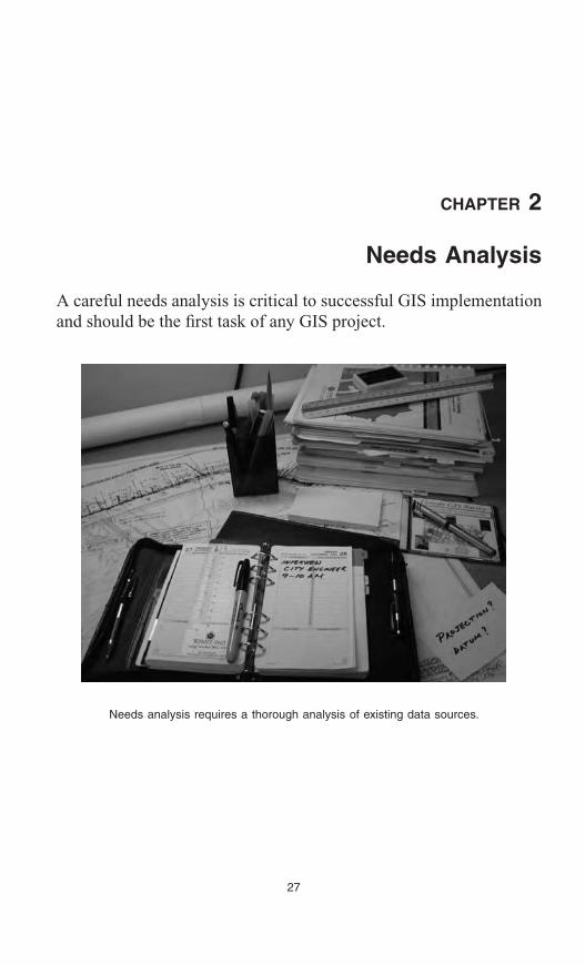
27
CHAPTER 2
Needs Analysis
A careful needs analysis is critical to successful GIS implementationand should be the first task of any GIS project.
Needs analysis requires a thorough analysis of existing data sources.

28 GIS APPLICATIONS FOR WATER, WASTEWATER, AND STORMWATER SYSTEMS
LEARNING OBJECTIVE
The learning objective of this chapter is to understand the value and methodologyof needs analysis for GIS application projects.
MAJOR TOPICS
• Definition of needs analysis• Needs analysis steps• Needs analysis case studies
LIST OF CHAPTER ACRONYMS
COTS Commercial Off-the-ShelfDBMS Database Management SystemGUI Graphical User InterfaceIT Information TechnologyRDBMS Relational Database Management System
OCEAN COUNTY’S STRATEGIC PLAN
Ocean County Utilities Authority, located in central New Jersey, serves 36municipalities through three wastewater treatment plants with a combined capacityof 80 MGD. The sewage collection system consists of 200 mi of sewer lines and40 pumping stations. The Authority developed a GIS program as an integral partof its information technology (IT) strategy. Instead of treating the GIS as a stand-alone system, the Authority envisioned using it as integrated part of its otherenterprise systems such as the SAP Maintenance Management System. Authority’sIT-based approach included the following steps (Stupar et al., 2002):
• Needs analysis: This step identified goals of the GIS as they related to theAuthority’s business needs.
• Spatial database design: The objective of this step was to treat GIS data as anenterprise asset. ESRI’s geodatabase data model was used to design the database.
• Data conversion: This step involved collecting the needed data and converting itto a geodatabase.
• Application development: This step designed and implemented applications forthe GIS.
INTRODUCTION
Needs analysis (or needs assessment) identifies and quantifies the GIS needs ofan organization and its stakeholders. Performing a needs analysis is the crucial firststep to a successful GIS project. Needs analysis is analogous to strategic planning;it is a blueprint for funding, implementing, and managing a GIS. Like strategicplanning, a careful needs analysis is critical to a successful GIS implementation and
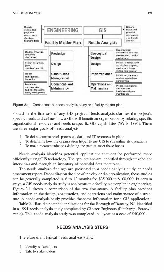
NEEDS ANALYSIS 29
should be the first task of any GIS project. Needs analysis clarifies the project’sspecific needs and defines how a GIS will benefit an organization by relating specificorganizational resources and needs to specific GIS capabilities (Wells, 1991). Thereare three major goals of needs analysis:
1. To define current work processes, data, and IT resources in place2. To determine how the organization hopes to use GIS to streamline its operations3. To make recommendations defining the path to meet these hopes
Needs analysis identifies potential applications that can be performed moreefficiently using GIS technology. The applications are identified through stakeholderinterviews and through an inventory of potential data resources.
The needs analysis findings are presented in a needs analysis study or needsassessment report. Depending on the size of the city or the organization, these studiescan be generally completed in 6 to 12 months for $25,000 to $100,000. In certainways, a GIS needs analysis study is analogous to a facility master plan in engineering.Figure 2.1 shows a comparison of the two documents. A facility plan providesinformation on the design, construction, and operations and maintenance of a struc-ture. A needs analysis study provides the same information for a GIS application.
Table 2.1 lists the potential applications for the Borough of Ramsey, NJ, identifiedin a 1994 needs analysis study completed by Chester Engineers (Pittsburgh, Pennsyl-vania). This needs analysis study was completed in 1 year at a cost of $40,000.
NEEDS ANALYSIS STEPS
There are eight typical needs analysis steps:
1. Identify stakeholders2. Talk to stakeholders
Figure 2.1 Comparison of needs-analysis study and facility master plan.

30 GIS APPLICATIONS FOR WATER, WASTEWATER, AND STORMWATER SYSTEMS
3. Inventory resources4. Establish need priorities5. Create system design6. Conduct a pilot project7. Prepare an implementation plan8. Conduct the final presentation
Step 1. Stakeholder Identification
Stakeholders include all the people who can affect or can be affected by a GISproject, such as users, executives, and GIS team members. A broader classificationcan include users, managers, IT personnel, customers, clients, policymakers, electedofficials, politicians, regulators, partners, and funding experts.
Step 2. Stakeholder Communication
This step requires talking with and listening to stakeholders to identify their GISneeds. Some or all of the following formal communication methods can beemployed:
1. Introductory seminar2. Work sessions3. Focus groups4. Interviews
Table 2.1 Potential Applications of GIS Technology
Department Representative Applications
Public works (responsible for operationand maintenance of the sewer system)
Emergency repairUtility markoutAsset managementMaintenance tracking and schedulingOne-call supportCritical water user locationWellhead protection
Engineering and planning Generation of 200-ft notification listsDemographic analysisPlanning reviewPermit approvalGreen space analysisFloodplain mappingDrainage management (storm sewer maps)
Tax office Parcel location and data retrievalTax-map productionProperty photo storage and retrievalAutomated public access
Public safety Fire hazard locationsHazardous-materials inventoryHydrant flow data retrievalPreferred hydrant locationCrime location analysis

NEEDS ANALYSIS 31
The first three methods are optional and can be used depending on the size,scope, and budget of the project. The last method is almost always necessary toperform a comprehensive needs analysis study.
Introductory Seminar
An introductory seminar is warranted if most of the stakeholders are new to GIS.It should focus on three critical questions:
1. What is GIS?2. Why use GIS?3. Who else is using GIS?
The first item defines GIS for those new to it. This part should be done inlayperson’s language. Avoid technical terms and acronyms typically found in acollege lecture on GIS-101. The second item answers the question of why GIS isimportant. It should emphasize that GIS benefits people, it makes things easier todo, and it increases productivity and reduces the cost of business functions. Thethird item presents compelling examples and success stories from other communitiesand organizations, such as:
• By using GIS, Charlotte, North Carolina, completed an H&H modeling projectinitially estimated at $1 million for less than $100,000.
• By using GIS and LIDAR elevation data, Chatham County, Georgia, saved $7 mil-lion in construction cost.
• By using GIS, Cincinnati, Ohio, expects to save $11 million in 15 years on awater infrastructure improvement project.
Success stories and associated savings factors presented in Chapter 1 (GISApplications) can be used to answer questions 2 and 3.
Work Sessions and Focus Groups
These 1- to 2-h management level focus group sessions are conducted to gain atop–down view of the issues confronting the organization. They also allow captureof the business processes that can be enhanced using GIS applications. The discus-sions lead to establishing goals that can be forged into benchmarks for GIS imple-mentation, such as:
• Creation of a map showing sewer pipes and manholes on an aerial photograph• Creation of a map showing water mains, fire hydrants, and valves on city streets• An application running on field (mobile) computers capable of identifying valves
that should be closed to isolate a broken water main for repair
Interviews
This is often considered the single most important step in the development of aGIS plan (Henstridge, 1998). A number of selected stakeholders should be inter-viewed to identify the needs, uses, problems, and requirements the organization has
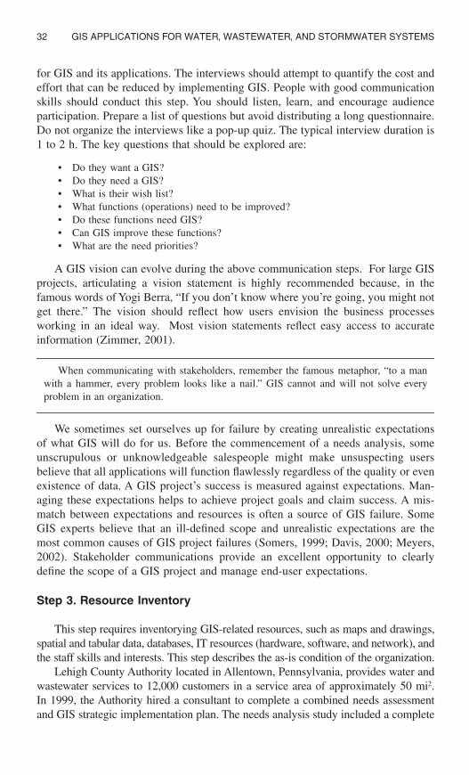
32 GIS APPLICATIONS FOR WATER, WASTEWATER, AND STORMWATER SYSTEMS
for GIS and its applications. The interviews should attempt to quantify the cost andeffort that can be reduced by implementing GIS. People with good communicationskills should conduct this step. You should listen, learn, and encourage audienceparticipation. Prepare a list of questions but avoid distributing a long questionnaire.Do not organize the interviews like a pop-up quiz. The typical interview duration is1 to 2 h. The key questions that should be explored are:
• Do they want a GIS?• Do they need a GIS?• What is their wish list?• What functions (operations) need to be improved?• Do these functions need GIS?• Can GIS improve these functions?• What are the need priorities?
A GIS vision can evolve during the above communication steps. For large GISprojects, articulating a vision statement is highly recommended because, in thefamous words of Yogi Berra, “If you don’t know where you’re going, you might notget there.” The vision should reflect how users envision the business processesworking in an ideal way. Most vision statements reflect easy access to accurateinformation (Zimmer, 2001).
When communicating with stakeholders, remember the famous
metaphor, “to a manwith a hammer, every problem looks like a nail.” GIS cannot and will not solve everyproblem in an organization.
We sometimes set ourselves up for failure by creating unrealistic expectationsof what GIS will do for us. Before the commencement of a needs analysis, someunscrupulous or unknowledgeable salespeople might make unsuspecting usersbelieve that all applications will function flawlessly regardless of the quality or evenexistence of data. A GIS project’s success is measured against expectations. Man-aging these expectations helps to achieve project goals and claim success. A mis-match between expectations and resources is often a source of GIS failure. SomeGIS experts believe that an ill-defined scope and unrealistic expectations are themost common causes of GIS project failures (Somers, 1999; Davis, 2000; Meyers,2002). Stakeholder communications provide an excellent opportunity to clearlydefine the scope of a GIS project and manage end-user expectations.
Step 3. Resource Inventory
This step requires inventorying GIS-related resources, such as maps and drawings,spatial and tabular data, databases, IT resources (hardware, software, and network), andthe staff skills and interests. This step describes the as-is condition of the organization.
Lehigh County Authority located in Allentown, Pennsylvania, provides water andwastewater services to 12,000 customers in a service area of approximately 50 mi2.In 1999, the Authority hired a consultant to complete a combined needs assessmentand GIS strategic implementation plan. The needs analysis study included a complete

NEEDS ANALYSIS 33
inventory of the Authority’s digital and hard-copy data sources and compiled thefollowing list (Babbitt, 2002):
• A 1-in. = 800-ft schematic map• A series of valve maps for each development• Some CAD files• Approximately 900 as-built drawings• A valve and hydrant database in Microsoft Access• An in-house customer information system in the ADMINS language
Step 4. Need Priorities
Because it is not feasible to implement a large number of applications simulta-neously, the needs identified in Step 1 should be prioritized. This can be done byassigning a priority ranking to needs, such as mission critical, most urgent, very high,high, medium, and low. For example, Lehigh County Authority’s needs analysis studyidentified 34 potential applications. Of these, five were considered high priority basedon organization-wide use and business process improvements (Babbitt, 2002).
Remember that the people who are paying for your GIS project would be anxiousto see the return on their investment. Applications that can be developed quickly(e.g., digital orthophotos) should, therefore, be given a higher priority to help showearly progress during the implementation phase. The applications that are least costlyor those that give the “biggest bang for the buck” (e.g., downloadable digital elevationmodels) can also be assigned a higher priority.
A common approach to implementing this step is to summarize and correlate theinterview results into a matrix with priorities assigned to each need. Table 2.2 showsa popular method to quantify the needs by preparing a matrix of needs (applications)and the departments that need those applications. The last column shows the totalscore of each identified need as the sum of departments requiring that need.
Step 5. System Design
This step recommends a GIS to support the applications identified in the previoussteps. It should evaluate the as-is state of the organization relative to key businessfunctions and identify the required elements needed to create the desired improvements.System design includes determining specifications for the following components:
• Data conversion (mapping)• Database• Software• Hardware• User interface
Data Conversion (Mapping)
Approximately 75% of typical GIS costs are related to data conversion and cre-ation. This component includes data conversion methods (scanning, digitization, etc.)

34 GIS APPLICATIONS FOR WATER, WASTEWATER, AND STORMWATER SYSTEMS
and the source, resolution, and scale of the maps or map layers. Needs-driven designis particularly critical for data conversion and database components. The design andcontent of the mapping and database components determine the fundamental capa-bilities of the entire GIS. These components can be considered to be the foundationof the system. Once actual implementation has begun, extensive changes to eitherthe mapping or the database design can be very costly. Additional information forthis component is provided in Chapter 8 (Mapping).
Database
A GIS database stores descriptive information about map features as attributes. Forexample, a water system database includes attributes for pipes, valves, meters, hydrants,and so on; and a sewer system database contains attributes for pipes, manholes, catchbasins, outfalls, and so on. The creation of an appropriate GIS database is the mostdifficult and expensive part of developing GIS applications. Successful GIS applicationsrequire a database that provides appropriate information in a useful and accessible form.The design of the database is, therefore, driven by application needs.
Table 2.2 Sample Departmental Needs Matrix
Needs (Applications)
Departments
Tota
l S
core
Ad
min
istr
atio
n
Pla
nts
Cu
sto
mer
Ser
vice
Lab
En
gin
eeri
ng
Co
llect
ion
Sys
tem
Sh
op
/Pu
rch
asin
g
Pre
trea
tmen
t
So
lids
Public access/general GISdata viewing
9
Emergency managementresponse
— — — — — 4
Special notification — — — — — 4
Customer location and service verification
— — — — — — — 2
Customer service/complaint tracking
— — — — — 4
Sample point monitoring andtracking
— — — — — — 3
As-built indexing — — — — — — — 2
Work order management — 8
Project management tracking — — — — — — — 2
Link TV inspections toGIS/work order management
— — — — — — — 2
Pretreatment tracking — — — — — 4
Biosolids tracking — — — — — — 3

NEEDS ANALYSIS 35
For data storage and manipulation, a database management system (DBMS) usesa data model, such as a hierarchical, network, or relational data model. ConventionalGIS databases consist of graphic features with links or pointers (usually facilityidentification numbers, or IDs) to related attribute or tabular data. In the late 1990s,a new object-oriented (rule-based) data model was introduced that stores attributesas an intrinsic part of the graphics feature. These modern databases do not requirelinks between features and attributes because they can store both the graphic featuresand attributes inside a single relational DBMS (RDBMS).
Database design involves three steps: (1) conceptual design, (2) logical design,and (3) physical design (Shamsi, 2002). Conceptual design does not depend onhardware or software. Logical design depends on software only. Physical designdepends on hardware and provides a detailed definition of the structure and contentof the database. Database design is presented with the help of a data dictionary,which documents the logical and physical structure of the layers of the GIS. Table 2.3shows a sample data dictionary for a 2000 sewer mapping project in the city ofMonongahela, Pennsylvania.
Table 2.3 Sample Data Dictionary
Layer Name Class Attribute Description
Study area STUDY Lines none Defines general study areaand clips other layers
City boundary BOUNDARY Lines none Municipal boundary
Roads ROADS Lines none City streets from CAD file
Railroads RAILS Lines none Railroads from TIGER file
Surface water RIVERS Lines none River and creeks fromCAD file
Subarea SUBAREA Lines
Polygons
none
Subarea_id
AcresMn_percimp
PopMn_popdenHousesMn_famsizeMn_mktvalMn_medinc
Digitized sewershedboundaries
Subarea identification(ID) number
Area in acresMean percentageimperviousness
PopulationMean population densityNumber of housesMean family sizeMean market valueMean median familyincome
Sewers SEWERS Lines None Collection system sewers
Interceptor INTERCEP Lines None Interceptor sewers
Treatment plant TREATMNT Lines None Treatment plant footprint
CSO dischargepoint
CSO Points Cso_id ID Number of combinedsewer overflow (CSO)discharge points

36 GIS APPLICATIONS FOR WATER, WASTEWATER, AND STORMWATER SYSTEMS
For detailed information on water, wastewater, and wastewater system databasedesign, please refer to the author’s companion book GIS Tools for Water, Wastewater,and Stormwater Systems (Shamsi, 2002).
Software Selection
GIS software represents less than 10% of the total GIS cost in most cases, yetpeople spend a lot of time in selecting the best software for their GIS applications.Many users are so proficient (and sometimes loyal) in using a given software thatthey will lose interest in GIS if they are not allowed to use their favorite GIS software.Because user needs are key to the success of a GIS project, their preferences shouldbe taken seriously. Thus, despite its relatively lower cost, GIS software can have asignificant impact on the success of a GIS project.
GIS software should have an “open” architecture. An open GIS allows for sharingof geographic data and integration among various GIS, GIS-related (e.g., remotesensing), and even non-GIS (e.g., hydraulic modeling) technologies. An open GIScan operate on different operating systems, platforms, and database managementsystems. It can be scaled to support a wide range of application needs, from an officeengineer using GIS on a desktop, to a mobile field technician using a handheld device,to hundreds of users working on an enterprise system across multiple departments.
Today, GIS development software used for data conversion work is almost alwaysa commercial off-the-shelf (COTS) program because custom development would besimply too expensive. Many commercial packages are available for implementingcommon GIS applications, such as work order management. Thus, no softwaredevelopment is necessary for data conversion or application software because rein-venting the wheel is “penny-wise and pound-foolish.” Some U.S. government agen-cies that invested in developing their own home-grown GIS packages did not see areturn on their investment (Henstridge, 1998a). Custom development is warrantedif COTS packages are not available for an application or if they are too expensive.As described in the following text, creation of a custom user interface also requiressoftware development.
Custom software can be developed in-house if computer programmers skilledin the GIS-specific programming languages are available. If this is not possible,consultants can be hired. Development and (often overlooked) maintenance costsare the major disadvantages of in-house development. For some organizations (e.g.,consultants) an advantage of the in-house software is the competitive edge of pro-prietary packages.
A needs analysis must carefully select an appropriate GIS software for the GISneeds of an organization. Fortunately, the field has narrowed and there are only afew major vendors today (Henstridge, 1998a). Some needs analysis studies utilizea decision matrix of user needs (applications) and available software capabilities tohelp select the most appropriate software. For example, Table 2.4 shows a sampledecision matrix for various applications of a typical water utility that uses an ESRIGIS platform. This table indicates that ArcView, ArcInfo, and Spatial DatabaseEngine (SDE) should be given high priority because they are required to implementall the GIS applications of the organization.

NEEDS ANALYSIS 37
Hardware Selection
The selection of appropriate GIS hardware depends on the scope of the GISapplication project and the available resources. GIS hardware can be set up as astand-alone workstation or in a network configuration. Typical hardware require-ments are listed in the following text:
• Computer with fast processor, large memory, and extensive disk space• DVD drive• Large-screen, high-resolution, color monitor (21 in. minimum)• Backup and storage device, such as a CD or DVD burner• Color printer• Large-format (wide-format) color plotter• Digitizer• Large-format scanner• High-speed Internet connection (T1, cable, or DSL)• GPS receiver• Computer server (for networked configurations)
Hardware can be expensive, but like the GIS software, the hardware for a typicalmunicipal GIS accounts for less than 10% of the total GIS investment. Thus, costalone should not be used in hardware selection. The following additional factorsshould also be considered: service and support, capacity for growth (storage andmemory), connectivity with peripheral devices (plotters, scanners, digitizers, GPSequipment, and field computers), and connectivity with Internet and networks (intra-nets and extranets). When comparing prices and hardware features, remember thegolden rule: You get what you pay for. Another valuable advice for hardwareprocurement is: Try before you buy.
Today’s laptops are just as powerful as desktops. For certain users, like a GISmanager who must commute between different offices, a laptop computer might bemore suitable than a desktop computer. The laptops cost more but are worth theextra money for mobile users. As of 2003, the minimum requirements for a laptopto be able to run GIS software are: a 1.7 GHz processor; 512 MB memory; 60 GBhard drive; 1280 x 1024 resolution, 32-bit color XGA screen; DVD R/RW drive;Internal 56K modem; and an Ethernet or wireless Local Area Network (LAN)(Thrall, 2003).
Table 2.4 Software Selection Matrix Example
Application AV SA NA 3DA AI SDE AO
Planning and engineering — —Operations and maintenance — —Construction — —Infrastructure management — —Water resources and hydrology — — —Finance and administration — — — —
Notes: AV = ArcView; SA = Spatial Analyst; NA = Network Analyst; 3DA = 3D Analyst;AI = ArcInfo; SDE = Spatial Database Engine; and AO = ArcObjects.
38 GIS APPLICATIONS FOR WATER, WASTEWATER, AND STORMWATER SYSTEMS
Client/server architecture is a common computer system configuration in whichone main server stores and distributes all data. Workstation users, called “clients,”access and manipulate server data using client software installed on the workstationcomputer. A network-based design is necessary if more than one person will needto access the same GIS data, i.e., when a team rather than an individual is workingon a project. For an individual researcher doing a thesis or term project, a personalworkstation is sufficient. However, in real-world projects the entire project teammust share the data, which requires a client/server architecture. Server maintenanceis absolutely necessary. Without a dedicated technician, the client/server architectureis difficult to maintain.
Wide- or large-format plotters allow printing on 24- to 60-in. rolls. Today’s wide-format plotters are available in both ink and laser technology. The cost depends onresolution, color, and speed. Common inkjet plotters range from $2,500 to $25,000.Common laser plotters range from $15,000 to $175,000. When budgeting for hardwarecost, do not forget to include the maintenance cost; for example, supplies for printerand scanner such as toner, ink cartridge, paper rolls, etc. Compare the up-front costof a laser printer to the savings of not replacing cartridges (approximately $40 each).The maintenance cost can range $100 to $500 per month based on usage. Thus, whenpricing a plotter, do not forget the cost of media and ink. Compare the plotters usinga cost-per-page figure for different media types. Make sure that the plotter you choosecan handle a large number of plots per day at the quality you prefer. Request for ademonstration and plot your own maps before making the final selection. Somemanufacturers like Hewlett Packard allow trading in the old plotter toward the purchaseof a new one and have lease options starting at less than $100 per month.
As of 2000, ESRI software runs on many platforms including Digital Tru64UNIX and Alpha Windows NT, IBM, AIX, HP-UX, Microsoft Windows95/98/NT/2000, NEC EWS-UX, SGI IRIX, and Sun Solaris. Linux is being evalu-ated and tested as a viable platform (ESRI, 2000).
Orange County Geomatics/Land Information Office started to provide enterprise-wide access to GIS data in 1997 using hardware and software from Intergraph. TheirOracle database containing 7 GB of attribute information resided on a 200 MHzQuad Pentium Pro with 256 MB of RAM. The data could be viewed using Inter-graph’s MGE product suite (Goldstein, 1997).
Table 2.5 provides sample hardware and software specifications for a single-userinstallation specified in a 1994 needs analysis study for the Borough of Ramsey, NewJersey. The 1994 cost for this setup was approximately $3000. Table 2.6 provideshardware and software specifications and the approximate cost specified in 2000 fora four-seat, server-based GIS laboratory. The 2000 cost for this setup was approxi-mately $145,000. A comparison of Table 2.5 and Table 2.6 indicates that computerhardware has changed substantially within the period of 6 years from 1994 to 2000.
User Interface
A user interface is a computer program that acts as an interpreter between theuser and a computer. It generally operates on top of a GIS package as a menu-drivenshell to the software’s commands. A graphical user interface (GUI) is a popular

NEEDS ANALYSIS 39
type of user interface that replaces difficult-to-remember text commands by inter-active computer graphics consisting of menus, dialogue boxes, input and outputwindows, and icons (Shamsi, 1997). For example, Internet Explorer™ is a GUI forthe World Wide Web.
Creation of a custom GUI is optional. It is recommended when the GIS functionsare very complex and/or the end users are complete novices. A custom GUI providesaccess (links) to all the GIS functions of an organization from a single program(screen) that bears the organization name and corporate logo. A custom GUI canalso be used for user authentication using passwords.
Table 2.5 Single-User Hardware and Software Specifications (Year 1994 Example)
Component Recommended Specifications
CPU Intel Pentium, 256 KB RAM cacheVideo card VL-bus Windows accelerator capable of 72 Hz vertical
refresh rate at 1024 x 768 resolution with 256 simultaneouscolors, noninterlaced
Monitor 17 in. size, performance to match video card, 0.28 mm dot pitchRAM 16 MB, expandable to 32 MB, 36-bit SIMMsHard drive 500 MB IDEFloppy drives One 3.5 in. (1.44 MB), one 5.25 in (1.2 MB)Expansion slots Eight ISA slots, including two VL-bus slotsDrive bays Total of five half-height bays, three with front accessFax modem 14,400 bps Hayes compatible, internalPrinter/plotter HP 650C DesignJetSoftware DOS 6.0, Windows 3.1, ArcView
Table 2.6 Hardware and Software Specifications, and Cost of a Four-User GIS Laboratory (Year 2000 Example)
ItemYear 2000Cost ($)
One 400 MHz Pentium II NT server with 256 MB100 MHz SDRAM, 3 x 4 GB hot swap hard drives,and Uninterruptible Power Supply (UPS)
9,000
Four Pentium II personal workstations (400 MHz,128 MB RAM, 4.3 GB hard disk, writeable CD-ROM) with 21 in. monitors ($4,000 per workstation)
16,000
UPS backup for all personal workstations ($300 each) 1,200Large-format color scanner with floor stand CalcompScanPlus III 800C (A–E size, 800 dpi max resolution)
20,000
Flatbed desktop scanner 100Digitizer (42 x 60 in.) with floor stand. Must be WinTabcompliant. Calcomp Summagrid V or GTCO Accutab.
10,000
Color plotter. Must be E size (36 in. wide). HP DesignJet750C Plus (36-in.-wide sheet roll)
7,500
B&W LaserJet printer (HP LaserJet 5 or better) 500Color inkjet desktop printer (HP DeskJet 1600C or better) 500Iomega 2 GB Jaz drive for backup 500ARC/INFO NT bundle 4 seats (includes ARC/INFO, ArcView,and ArcView extensions) ($20,000 each)
80,000
Total Cost 145,300

40 GIS APPLICATIONS FOR WATER, WASTEWATER, AND STORMWATER SYSTEMS
Some GIS packages allow customization of their default interfaces with little orno programming to meet user-specific needs. When available, this feature can beused to create simple GUIs. Custom GUIs for complex applications require computerprogramming or scripting. Custom GUI development needs will be graduallyreduced and eventually eliminated as GIS packages complete their migration froma command-based to an interface-based environment.
Step 6. Pilot Project
This is a very important step. Inclusion of a pilot project in a GIS implementationplan allows the project team to test an initial strategy before committing to a specificcourse of action. For example, database design determines the fundamental capa-bilities of the entire GIS. Once actual implementation has begun, extensive changesto database design are very costly. Thus, before a systemwide implementation, theinitial database design and data conversion methodology should be evaluated for asmall portion of the project area (pilot area). The pilot project allows you to test thesystem design, evaluate the results, and modify the system design if necessary. Itprovides an opportunity to refine the proposed approach to full-scale data conversionand implementation. This step should also produce a working demonstration of theintended applications for the pilot area.
The Washington Suburban Sanitary Authority (WSSC) is among the ten largestwater and wastewater utilities in the U.S. According to the 2003 records, it serves420,000 customer accounts, provides water and sewer services to 1.6 million resi-dents in a nearly 1000 mi2 area, and employs more than 1500 people. In the early1990s, WSSC undertook GIS implementation as a cooperative effort with five otherregional agencies. The interagency organization called Geographic Information Sys-tem for Montgomery and Prince George’s Counties (GeoMaP) proceeded withstudies to assess needs, analyze requirements, and evaluate alternatives. A detailedGIS system design was then completed for specifications of database, data conver-sion, hardware, software, and communications network. A pilot project was com-pleted to evaluate the system design prior to full-scale implementation. The pilotwas intended to be the first phase of GIS implementation rather than a separateexperimental effort or prototype. The pilot project developed all components of theproposed database design for sample areas and designed and developed a sampleset of GIS applications. The water and sewer facility layers were structured asARC/INFO network coverages to support network analysis applications as well asto provide standard water and sewer reference maps. The sewer layer was foundmuch easier to develop than the water layer (Cannistra et al., 1992).
Mohawk Valley Water (MVW) is a water utility serving more than 125,000people in approximately 150 mi2 area in central New York. MVW completed a 6-month pilot project in 2002 to develop a water distribution system geodatabase usingESRI’s ArcGIS, ArcIMS, and ArcSDE software and a hydraulic model using HaestadMethod’s WaterCAD software. The pilot project covered approximately 5% of therepresentative distribution system area including three storage tanks and two pump-ing stations. The database design used ESRI’s Water Distribution Data Model. Amajor goal of the pilot project was to estimate the time and money required to

NEEDS ANALYSIS 41
implement GIS and hydraulic modeling in the entire system (DeGironimo andSchoenberg, 2002). Another pilot project example, for the Borough of Ramsey, isdescribed later in this chapter.
Step 7. Implementation Plan
An implementation plan identifies specific actions and resources required toimplement a GIS. It provides information on schedule, cost, staffing, training, andoperation and maintenance. It is used by a project or program manager to build theGIS, so it should be as detailed as possible. Phased implementation is preferable.The phases should be designed to distribute the cost evenly and to allow a comfort-able pace over the project duration. Schedule success into your project schedule.Create your implementation plan with a few small but early successes to help yousustain the momentum over potential rough spots. Plan for early success by firstimplementing quick and high-impact applications that can be put to use right away.GIS integration with other information systems and applications (e.g., hydraulicmodeling) is beneficial but technically complex. Because clearly identifiable benefitsshould be achieved in the earlier phases of an implementation plan, integration tasksshould be scheduled for later phases where possible.
A successful implementation plan should be based on a holistic approach that achievesbalance among stakeholders, technology, time, and budget.
Define key success factors before starting. Treat the success factors — such asacquiring hardware, installing and testing software, conducting training and work-shops, populating the database, testing the database, and developing applications —as milestones. Project milestones provide a ruler against which success can bemeasured. Hitting these milestones will show the success of your GIS in clearlydemonstrable ways and will allow you to measure success in small steps along theway. The milestones should specify the data sets, applications, and user access. Amilestone like “Hydraulic Modeling by January 2004” leaves too much room forinterpretation and, thus, dissatisfaction. A more useful milestone would be “Linkingthe water layer to EPANET model for the Engineering Department by January 2004.”
User involvement is a key factor in the success of a GIS project. They shouldbe incorporated in all stages of GIS development, rather than only in the needsanalysis interviews. User training is paramount to the success of a GIS applicationproject after it has been implemented.
The implementation plan should identify GIS staffing needs. This requires under-standing the composition of the user community. When considering the best approachto GIS staffing and expertise investments, four factors should be evaluated: GIS expertiserequirements, GIS project situation (e.g., early or later project phases), internal envi-ronment (e.g., hiring policies and procedures), and external environment (e.g., jobmarket) (Somers, 1999a). All alternatives to fulfill GIS staffing needs including trainingexisting staff, hiring new personnel, and using contractors and consultants should beevaluated. In-house projects do not require capital funds, and internal staff is more

42 GIS APPLICATIONS FOR WATER, WASTEWATER, AND STORMWATER SYSTEMS
familiar with source documents. Contractors can usually complete the projects fasterbecause they have specialized experience, more workers, and higher productivity.
The long-term viability of a GIS requires ongoing maintenance. Maintenanceactivities include updating the GIS data layers to reflect changes such as new streets,subdivisions, or sewer lines. Such routine maintenance activities can be contractedout on an hourly basis. The typical data maintenance cost for medium-size commu-nities is $3000 to $5000 per year. The implementation plan should provide themaintenance procedure and responsibility for each layer in the GIS. For example,standards for site plans from developers and engineers should be developed so thatchanges can be easily incorporated into the GIS. Today, most plans are available inAutoCAD DXF or DWG file format and might require a data conversion effort forincorporating them into a GIS. For ESRI users, the Shapefile will be a more suitableformat for accepting the site plans. If required, multiple-user editing of GIS layersshould be provided by selecting appropriate GIS software. Separate operations andmaintenance (O&M) manuals should be developed for large installations.
Procedures for obtaining ongoing operations support should be recommended.Today, annual software support can be easily purchased with the software. On-site
Table 2.7 Implementation Priorities and Project Phases
Needs (Applications) Tota
l S
core
Co
st t
o I
mp
lem
ent
Dif
ficu
lty
to I
mp
lem
ent
Mis
sio
n C
riti
cal
Pro
ject
Ph
ase
Data Type
Public access/general GIS data viewing 9 L L VH 1 Core, facility,department
Work order management 8 M L VH 1 Core, facilityEmergency management response 4 M L H 1 Core, facilitySpecial notification 4 L L M 1 Core, facilityCustomer service/complaint tracking 4 M/L L H 1 Core, facilityPretreatment tracking 4 L L M 2 Core, facility,
departmentSample point monitoring and tracking 3 L L L 2 Core, facility,
departmentBiosolids tracking 3 L L L 2 Core, facility,
departmentCustomer location and serviceverification
2 M/L M H 1 Core, facility
As-built indexing 2 M M M 1 Core, facilityProject management tracking 2 M M/L M/L 2 Core, facility,
departmentLink TV inspections to GIS/work ordermanagement
2 M/H M/H M 1 Core, facility,department
Notes: L = low; M = medium; H = high; VH = very high; M/L = medium/low; and M/H =medium/high.

NEEDS ANALYSIS 43
troubleshooting support can be obtained from consultants on an hourly or incidentbasis.
Finally, perceptions and expectations and hence the needs of people often changewith time. A GIS implementation plan, especially if it is a long one, should beflexible to accommodate changes in organizations, people, and technology.
Table 2.7 shows a sample implementation plan summary. The first two columnsshow the needs and their scores from Table 2.2. Columns 3 to 5 assign rankingsbased on cost, implementation difficulty, and mission criticality, respectively. Thesixth column assigns a project phase based on columns 2 to 5. The last columnshows the data type required for each identified need.
Step 8. Final Presentation
This presentation should be conducted for the same audience that attended theintroductory seminar. It should summarize the findings of the needs analysis study.The presentation should also include a live demonstration of the pilot project.
NEEDS ANALYSIS EXAMPLES
Some needs analysis examples are given in the following subsections that dem-onstrate the results of conducting various needs analysis steps described in thepreceding text.
Pittsburgh, Pennsylvania
The city of Pittsburgh performed an in-house needs analysis in 1984 that spanneda period of 4 years and took 18 months of staff time (Wells, 1991). The heart ofthis needs analysis was a comprehensive inventory of existing files and maps. Theneeds analysis listed major functions and responsibilities of each city department.The major GIS applications included:
• Maintaining infrastructure maps and inventories• Allowing network tracing and analysis for water, sewer, and stormwater systems• A water and sewer facilities management system• Computing shortest routes for emergency response and work crews• Permit processing• Address matching• Producing maps• Enhancing property and business tax administration• Automating acquisition, maintenance, and disposal of tax-delinquent properties• Integrating census and municipal data for community planning and budget analysis• Facilitating production of routine reports, tables, form letters, and mailing lists• Creating and maintaining disaster preparedness map layers (hazardous-material
sites, hospitals, group care facilities, etc.)
Once the needs analysis was completed, the city hired a consultant (PlanGraph-ics, Inc.) to procure a GIS implementation project. The consultant translated thecity’s GIS needs into the following technical specifications:

44 GIS APPLICATIONS FOR WATER, WASTEWATER, AND STORMWATER SYSTEMS
• Database structure• Data entry• Graphic data manipulation• Database query• Data output and display• User-directed software development• System operation• Applications• System configuration and hardware
The consultant prepared a Request for Qualifications (RFQ) and Request forProposals (RFP). The RFQ was sent to 80 firms and the RFP was sent to 11 firms.The proposals were submitted by five vendors.
Borough of Ramsey, New Jersey
The Ramsey Board of Public Works is responsible for the operation andmaintenance of water distribution and sanitary sewer collection systems throughoutthe Borough of Ramsey. These operations necessitate the daily use of a variety ofmap products and associated geographically referenced (or “georeferenced”) infor-mation resources, which describe or are related to a specific location, such as aland parcel, manhole, sewer segment, or building. In an effort to more efficientlymanage its geographically referenced data, the board started to explore the benefitsand applications of GIS technology and computer mapping in early 1993. As afirst step, with the assistance of Chester Engineers, Inc. (Pittsburgh, Pennsylvania),they started a GIS pilot project (Shamsi et al., 1996). The goals of the pilot projectwere to:
• Thoroughly evaluate the benefits and costs of a GIS• Develop specifications for GIS implementation• Confirm the suitability of tasks selected for GIS automation• Demonstrate GIS functional capabilities• Firmly quantify unit costs of GIS implementation• Demonstrate GIS benefits to the departments not participating in the pilot project• Identify any technical problems• Provide immediate tangible benefits• Assess the quality of existing records and procedures
The GIS pilot project produced a GIS Needs Assessment Report, a GIS Imple-mentation Plan, and a functioning GIS demonstration system for a selected portionof the borough. With the knowledge and experience gained from the pilot project,the board was prepared to pursue a broader implementation of GIS technology.The geographic limits of the pilot project area were selected on the basis of twocriteria:
• Size: large enough to allow realistic evaluation, small enough to be affordable• Location: encompassing a portion of the borough where activities supported by
priority applications are likely to occur

NEEDS ANALYSIS 45
The selected pilot area measuring approximately 2600 ft × 2600 ft was locatedin the central portion of Ramsey. The pilot project was completed in 1 year forapproximately $40,000 (in 1994 dollars).
From the applications listed in Table 2.1, the following two priority applicationswere selected for pilot testing:
1. Public Works Department: Management of infrastructure asset location informationto support emergency repair and utility markout functions. The GIS will automatethe storage and retrieval of location and maintenance data for water and sewerinfrastructure. Expected benefits include more rapid emergency repair response,more efficient utility markouts, and more efficient scheduling of routine maintenance.
2. Planning Department: Generation of 200-ft notification lists as part of plan reviewprocess. GIS automation will generate a 200-ft buffer, identify affected parcels,retrieve lot and block numbers, retrieve property owner names and addresses, andprint a notification list. GIS benefits are expected to dramatically reduce the timerequired to complete these tasks.
The City of Bloomington, Indiana
The City of Bloomington (with a population of approximately 60,000) startedtheir GIS strategy with a needs analysis in 1989. They completed their base map bythe end of 1993, and got the system fully functional in the next year. They stored theGIS map and Oracle RDBMS data on workstations located at Bloomington’s UtilitiesService Center and distributed them through a fiber-optic network to city hall and topolice and fire departments. The GIS software was loaded on ten Unix workstationhost machines, most of which supported a number of X-terminal and P users acrossthe network (Goldstein, 1997).
San Mateo County, California
San Mateo County, also referred to as the “Gateway to Silicon Valley,” hasapproximately 200,000 property parcels and covers 552 mi2. In 2001, the countystarted development of an enterprise-wide GIS base map. A success factor for theproject was that all aspects of its development were planned and agreed on by allthe stakeholders before the project started. A GIS Steering Committee, in consulta-tion with a larger group of county departments, hired a consultant (GIS Consultants,Inc.) to conduct a needs analysis, which resulted in a strategic plan. Thereafter, aspecific implementation plan was designed for base-map construction, followed bydetailed and complete specifications and preliminary cost estimates. Formal needsanalysis efforts were credited for the timely completion of base-map creation, hard-ware and software purchase, and training (Joffe et al., 2001).
CHAPTER SUMMARY
This chapter described the importance and benefits of a needs analysis prior toimplementing a full-scale GIS project. Various steps involved in needs analysis wereexplained. When carefully done, needs analysis clarifies the project’s specific needs,

46 GIS APPLICATIONS FOR WATER, WASTEWATER, AND STORMWATER SYSTEMS
provides a process for arriving at interdepartmental understandings about the objec-tives and limits of a project, and establishes a detailed basis for developing GISmaps and applications.
CHAPTER QUESTIONS
1. What is needs analysis? How does it compare to strategic planning and facilitymaster planning?
2. What steps are recommended for needs analysis? Which step is most critical?3. What is a pilot project? What are the benefits of conducting a pilot project?4. How would you prepare a needs analysis study for a water system mapping
project?5. You are tasked with integrating a large city’s H&H model with the city’s GIS.
What will be your first step and why?

47
CHAPTER 3
Remote Sensing Applications
Can a satellite 400 miles above the ground surface help you locate aleaking pipe? Read this chapter to find out.
The Landsat 7 Enhanced Thematic Mapper (ETM+) scene of the lower Chesapeake Bay regionacquired on July 5, 1999 (Image courtesy of USGS).

48 GIS APPLICATIONS FOR WATER, WASTEWATER, AND STORMWATER SYSTEMS
LEARNING OBJECTIVE
The learning objective of this chapter is to comprehend the applications of remotesensing technology in the water industry.
MAJOR TOPICS
• Remote sensing satellites• Applications of satellite imagery• Types of remote sensing data• Digital orthophotos• Using remote sensing for land-use classification• Image processing software• Anticipated future trends
LIST OF CHAPTER ACRONYMS
DEM Digital Elevation ModelDOP Digital OrthophotoDOQ Digital Orthophoto QuadrangleDOQQ Digital Orthophoto Quarter QuadrangleLIDAR Laser Imaging Detection and RangingLULC Land Use/Land CoverTM Thematic Mapper (onboard Landsat satellite)USGS United States Geological Survey
ALBANY COUNTY’S REMOTE SENSING APPLICATION
Public-domain digital aerial photography data, such as USGS digital orthophotoquadrangles (DOQs) and digital orthophoto quarter quadrangles (DOQQs), usuallybecome outdated in rapidly developing areas. For such areas, high-resolution satelliteimagery may be a cost-effective source of more recent overhead images.
Albany County, located in southeastern Wyoming, covers 4,400 mi2, has a stu-dent-based population of 30,000, and has 1,600 mi of roads. For rural communitiessuch as Albany County, building a GIS from scratch can be an expensive endeavordue to lack of resources. The County’s day-to-day mapping functions required a datalayer of imagery for the entire county. Various data options were reviewed, includingaerial flights, existing DOQs, and satellite imagery. New aerial imagery was elimi-nated because it was too expensive. Existing DOQs were not suitable because theywere 7 years old and did not reflect recent county growth trends. In addition, costsassociated with updating the County’s existing digital aerial photography exceeded$100,000. High-resolution satellite imagery, on the other hand, allowed the Countyto have high-resolution up-to-date views of the entire county for $32,000. For 85mi2 of populated areas, the County selected 1-m pan-sharpened IKONOS satelliteimagery (described later in this chapter). For the rest of the county, 90 quads of

REMOTE SENSING APPLICATIONS 49
CARTERRA DOQ 5-m black and white (B&W) imagery was selected. Both productswere produced by Space Imaging (Thornton, Colorado). Thanks to this geographic-imaging approach, planning tasks previously requiring months to complete took onlydays after the County implemented this project (Frank, 2001).
In the Albany County of Wyoming, addition of high-resolution up-to-date imagery toGIS data reduced the completion of typical planning tasks from months to a few days.
INTRODUCTION
The technologies that are commonly used in conjunction with GIS are commonlyreferred to as GIS-related technologies. Examples include remote sensing, globalpositioning system (GPS) surveying, the Internet, and wireless technologies. Thischapter will focus on remote sensing, one of the most successful GIS-related-technologies. Other related technologies are described elsewhere in the book.
Remote sensing allows obtaining data of a process from a location far away fromthe user. Remote sensing can, therefore, be defined as a data collection method thatdoes not require direct observation by people. Remote sensing is the process ofdetection, identification, and analysis of objects through the use of sensors locatedremotely from the object. Three types of remote sensing systems are useful in thewater industry:
1. Aerial photographs2. Satellite imagery3. Radar imagery
The data from these systems are commonly referred to as remote sensing orremotely sensed data. Sometimes, remote sensing data are incorrectly confused withsupervisory control and data acquisition (SCADA) data used to operate water andwastewater treatment plants. Remote sensing data collected using airplanes are calledaerial photographs or aerial photos. Digital remote sensing data collected fromsatellites are called satellite imagery or images. Digital pictures of the Earth aretaken by satellites from 400 to 500 mi above the ground compared with aerialphotographs that are taken by aircraft from 1 mi above the ground (for low-altitudephotography) to 7 to 8 mi above the ground (for high-altitude photography). Thechart in Figure 3.1 shows the altitude difference between the aircraft- and satellite-type remote sensing systems. Radar imagery or images are another type of remotesensing data but their usage is not widespread in the water industry. Although thedefinition of remote sensing includes aerial photos and radar data, remote sensingis often considered synonymous with satellite imagery.
The American Society for Photogrammetry and Remote Sensing (ASPRS) valuesthe U.S. remote sensing industry at about $1.3 billion (as of 2001) and forecasts 13%annual growth, giving values of $3.4 billion by 2005 and $6 billion by 2010. Theindustry currently consists of about 220 core companies employing about 200,000employees in the areas of remote sensing, photogrammetry, and GIS imaging. A 2001

50 GIS APPLICATIONS FOR WATER, WASTEWATER, AND STORMWATER SYSTEMS
ASPRS study concludes that utilities are one of the greatest untapped potentialmarkets and that a shortage of trained workers is one of the greatest challenges tothe growth of the remote sensing industry (Barnes, 2001a).
Although vector GIS data are still an important and vital tool for many waterindustry applications, the newer raster GIS applications of satellite imagery arebeginning to make a major move into the GIS and mapping market. The benefits ofsatellite imagery are (Schultz, 1988):
1. They enable aerial measurements in place of point measurements.2. They offer high spatial and/or temporal resolution.3. All information is collected and stored at one place.4. Data are available in digital form.5. Data acquisition does not interfere with data observation.6. Data can be gathered for remote areas that are otherwise inaccessible.7. Once the remote sensing networks are installed, data measurement is relatively
inexpensive.
Satellite imagery is stored in a pixel (raster) format that makes it ideally suitedfor incorporation into a GIS (Engman, 1993). Thus, satellite imagery can be treatedas raster-type GIS data. Image processing equipment and methods can be used to
Figure 3.1 Altitude difference in aerial photography and satellite imagery.
1 mi
7–8 mi
400–500mi
Low Altitude High Altitude Satellite
1
10
100
1000
Remote Sensing System Type
Alti
tude
(m
iles)

REMOTE SENSING APPLICATIONS 51
extract useful information from hard copy and digital images and combine it withother data layers in a GIS. Image data sources including scanned paper maps, aerialphotographs, and satellite imagery can be used in a GIS when reprojected as imagemaps. Projected images can be used as a background or as a base map upon whichother vector layers are overlaid.
Casual GIS users can easily import remote sensing imagery into their GISprojects as an image theme (or layer). However, advanced remote sensing applica-tions and image analyses require formal remote sensing training and digital imageprocessing skills. The incorporation of remote sensing data in a GIS requires a digitalimage processing software such as ERDAS IMAGINE, Geomatica, ER Mapper, orENVI, or a raster GIS software with image processing capability, such as ArcGRIDor IDRISI. Such programs are described later in this chapter.
These are exciting times both for the GIS and the remote sensing industries,thanks to dramatic price and performance breakthroughs in GIS hardware andsoftware. The increasing use of GIS is contributing to a renewed interest in satelliteimagery by nongeographers, such as civil and environmental engineers. AlthoughGIS technology is promoting the use of satellite imagery, satellite imagery is alsoin turn advancing the use of GIS. Although non-GIS stand-alone image processingsoftware can be used for exploring satellite imagery, those with GIS capabilities aremore suitable because they can combine imagery with additional information, suchas demographic and topographic data (Corbley, 2000).
REMOTE SENSING APPLICATIONS
Satellite imagery is not restricted to the visible (0.4 to 0.7 µm wavelength) partof the electromagnetic spectrum. Satellite sensors can record Earth images at wave-lengths not visible to the human eye, such as near-infrared and thermal-infraredbands. Different satellite bands provide information about different objects andconditions of the Earth. For example, thermal-infrared band (10.4 to 12.5 µm wave-length) data are useful for soil–moisture discrimination. These bands of satellite datacan be used as different data layers in a GIS for further analysis.
Remote sensing applications in the water industry are as diverse and numerousas the GIS applications themselves. Typical examples are listed below:
1. Satellite remote sensing has contributed to water resources applications and researchfor three decades (Jackson, 2000). Remote sensing data are especially useful inwatershed hydrologic modeling. Satellite imagery can be used to estimate inputparameters for both the lumped-parameter and distributed-type hydrologic models.
2. Satellite imagery can be used for delineating watersheds and streams. For example,SPOT satellite’s stereographic capability can generate topographic data. Terrasatellite can provide digital elevation models (DEMs) from stereo images. (Theseand other satellites are discussed later in this chapter.) Topographic and DEM datacollected by satellites can be processed in GIS for automatic delineation of water-shed boundaries and streams.
3. Remote sensing data are used for land-use classification. GIS can help to refineor verify the imagery-based land-use classes.

52 GIS APPLICATIONS FOR WATER, WASTEWATER, AND STORMWATER SYSTEMS
4. Satellite and radar data can be used to estimate the area and intensity of rainfall.5. Remote sensing can produce surface temperature data through thermal-infrared
images.6. Microwave remote sensing can produce soil-moisture data.7. Remotely sensed temperature and moisture data can be combined to estimate
evaporation and evapotranspiration rates.8. Remote sensing data are used to estimate vegetation indices and the leaf area
index. These parameters can be combined to delineate areas where a subsurfacesupply of water is available for vegetation.
9. Remote sensing can be used in real time flood forecasting with a distributedhydrologic model into which radar rainfall data can be input.
10. Other applications (Singh, 1995; ASCE, 1999) are:• Utility routing• Weather forecasting• Environmental impact assessment of large water resources projects• Snow and ice conditions (microwave region)• Forecasting seasonal and short-term snowmelt runoff• Evaluation of watershed management strategies for conservation planning• Inventory surface water, such as rivers, lakes, reservoirs, swamps, and flooded
areas• Water quality parameters such as algae, chlorophyll, and aquatic life• Thermal and chemical pollution and oil spills• Drought assessment and forecasting• Geologic and geomorphologic information• Groundwater mapping
REMOTE SENSING SATELLITES
Satellite data became available to water industry professionals in 1972 when theU.S. government launched the first Landsat satellite, which was specifically designedto provide imagery of the Earth (Miotto, 2000). In the late 1970s and early 1980s,a second generation of Landsat satellites was developed. Landsats 4 and 5 werelaunched in July 1982 and March 1984, respectively. They were equipped with twoinstruments:
• Multispectral scanner (MSS) having 80-m resolution and 4 spectral bands• Thematic mapper (TM) having 30-m resolution and 7 spectral bands
MSS sensors capture imagery at different wavelengths of light to produce colorimages. Landsat 4 was retired in 1991, and Landsat 5’s MSS sensor failed in October1993. The successor satellite, Landsat 6, failed to achieve orbit in 1993. To keep theimagery flowing, Landsat 7 was launched on April 15, 1999.
Popular satellite-based sensors and platforms include Landsat MSS and TM,AVHRR, AVIRIS, SPOT XS, GOES, SEASAT, SIR, RADARSAT, SRTM, TOPSAT,ERS-1 and 2, and JERS-1 (Luce, 2001; Lunetta and Elvidge, 1998). The remotesensors that provide hydrologically useful data include aerial photographs, scanningradiometers, spectrometers, and microwave radars. The satellites that provide hydro-logically useful data are the NOAA series, TIROS N, SPOT, Landsat, and the
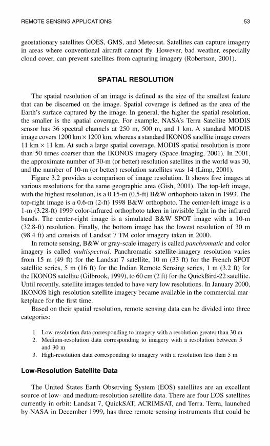
REMOTE SENSING APPLICATIONS 53
geostationary satellites GOES, GMS, and Meteosat. Satellites can capture imageryin areas where conventional aircraft cannot fly. However, bad weather, especiallycloud cover, can prevent satellites from capturing imagery (Robertson, 2001).
SPATIAL RESOLUTION
The spatial resolution of an image is defined as the size of the smallest featurethat can be discerned on the image. Spatial coverage is defined as the area of theEarth’s surface captured by the image. In general, the higher the spatial resolution,the smaller is the spatial coverage. For example, NASA’s Terra Satellite MODISsensor has 36 spectral channels at 250 m, 500 m, and 1 km. A standard MODISimage covers 1200 km
× 1200 km, whereas a standard IKONOS satellite image covers11 km
× 11 km. At such a large spatial coverage, MODIS spatial resolution is morethan 50 times coarser than the IKONOS imagery (Space Imaging, 2001). In 2001,the approximate number of 30-m (or better) resolution satellites in the world was 30,and the number of 10-m (or better) resolution satellites was 14 (Limp, 2001).
Figure 3.2 provides a comparison of image resolution. It shows five images atvarious resolutions for the same geographic area (Gish, 2001). The top-left image,with the highest resolution, is a 0.15-m (0.5-ft) B&W orthophoto taken in 1993. Thetop-right image is a 0.6-m (2-ft) 1998 B&W orthophoto. The center-left image is a1-m (3.28-ft) 1999 color-infrared orthophoto taken in invisible light in the infraredbands. The center-right image is a simulated B&W SPOT image with a 10-m(32.8-ft) resolution. Finally, the bottom image has the lowest resolution of 30 m(98.4 ft) and consists of Landsat 7 TM color imagery taken in 2000.
In remote sensing, B&W or gray-scale imagery is called panchromatic and colorimagery is called multispectral. Panchromatic satellite-imagery resolution variesfrom 15 m (49 ft) for the Landsat 7 satellite, 10 m (33 ft) for the French SPOTsatellite series, 5 m (16 ft) for the Indian Remote Sensing series, 1 m (3.2 ft) forthe IKONOS satellite (Gilbrook, 1999), to 60 cm (2 ft) for the QuickBird-22 satellite.Until recently, satellite images tended to have very low resolutions. In January 2000,IKONOS high-resolution satellite imagery became available in the commercial mar-ketplace for the first time.
Based on their spatial resolution, remote sensing data can be divided into threecategories:
1. Low-resolution data corresponding to imagery with a resolution greater than 30 m2. Medium-resolution data corresponding to imagery with a resolution between 5
and 30 m3. High-resolution data corresponding to imagery with a resolution less than 5 m
Low-Resolution Satellite Data
The United States Earth Observing System (EOS) satellites are an excellentsource of low- and medium-resolution satellite data. There are four EOS satellitescurrently in orbit: Landsat 7, QuickSAT, ACRIMSAT, and Terra. Terra, launchedby NASA in December 1999, has three remote sensing instruments that could be

54 GIS APPLICATIONS FOR WATER, WASTEWATER, AND STORMWATER SYSTEMS
useful for certain water resources applications: Advanced Spaceborne ThermalEmission and Reflection Radiometer (ASTER), Moderate Resolution Imaging Spec-troradiometer (MODIS), and Multiangle Imaging Spectroradiometer (MISR). ASTERprovides digital elevation maps prepared from stereo images. MODIS provides dataon cloud- and snow-cover characteristics. MISR data can distinguish different typesof clouds, land cover, and vegetation canopy. Although low-resolution satellite imageryworks well for regional level studies, it is not very useful in water industry applications.
Medium-Resolution Satellite Data
Table 3.1 provides a summary of medium-resolution satellites. Landsat 7 is themost recent satellite in the Landsat series. By May 2001, Landsat 7 had capturedmore than 200,000 15-m scenes throughout the world. The Enhanced Thematic
Figure 3.2 Image resolution comparison. Top left: 0.15-m B&W orthophoto (1993); top right:0.6-m B&W orthophoto (1998); center left: 1-m color infrared orthophoto (1999);center right: 10-m simulated SPOT; bottom: 30-m Landsat TM (2000).

REMOTE SENSING APPLICATIONS 55
Mapper Plus (ETM+) sensor onboard Landsat 7 provides 15-m panchromatic and30-m multispectral resolutions. Landsat 7 offers imagery of the highest resolutionand lowest price of any Landsat. The USGS ground-receiving station in Sioux Falls,South Dakota, records 250 Landsat scenes a day that are available online within 24hours. Landsat 7 is expected to have a design life of 5 years. Each Landsat imagecovers about 10,000 mi2. Landsat 7 is very useful in water resources applications.
Figure 3.3 shows a modified Landsat TM image for southwestern Pennsylvania,which can be used in a GIS to consistently map land use/land cover (LULC)throughout the state. These images, called Terrabyte, are extracted from the 30-mresolution TM data using an extractive process based on a research trust at PennState University under cooperation between the Office for Remote Sensing of EarthResources in the Environmental Resources Research Institute and the Center for
Table 3.1 List of Major Medium-Resolution Satellites
Feature Landsat 7 SPOT 4 IRS-1C
Company USGS French Government Indian GovernmentLaunch date April 15, 1999 1998 December 28, 1995B&W resolution 15 10 5Color resolution 30 20 23Swath width (km) 185 120 70Global cover repeat days 16 26 24
Figure 3.3 Terrabyte Landsat Thematic Mapper image for southwestern Pennsylvania.

56 GIS APPLICATIONS FOR WATER, WASTEWATER, AND STORMWATER SYSTEMS
Statistical Ecology and Environmental Statistics in the Department of Statistics, withsponsorship from the National Science Foundation and the Environmental ProtectionAgency. The Terrabyte images are not intended to provide fine detail such as indi-vidual buildings at the site level, but rather to convey a sense of landscape organi-zation. Each pixel record occupies one byte; hence the name Terrabyte. Terrabytecondensations for ten satellite scenes will fit on one CD-ROM, whereas two scenesof original satellite data would more than fill one CD-ROM. Terrabyte CD-ROMsof Pennsylvania data have been distributed by Pennsylvania Mapping and Geo-graphic Information Consortium (PaMAGIC) (www.pamagic.org).
In addition to the EOS satellites, France’s SPOT 4 satellite provides 10-mpanchromatic and 20-m color imagery. In the U.S., 60
× 60 km SPOT scenes cost$750 (pre-1998) to $1500 (post-1998). India’s Indian Remote Sensing (IRS) satelliteIRS-1C provides 5-m panchromatic and 23-m or 188-m color imagery. Commercialcompanies and government agencies around the world had plans to launch morethan 25 medium-resolution (30 m or better) satellites by the end of 2003.
High-Resolution Satellite Data
High-resolution data correspond to imagery whose resolution is less than 5 m.Traditionally, water industry professionals have purchased aerial photography serviceson an as-needed basis, which is costly and time-consuming. Now, thousands of squaremiles of GIS-ready seamless imagery is available in various formats with the promiseto bring remote sensing data to any desktop (Robertson, 2001). Until recently, somewater industry professionals used 5-m panchromatic imagery from India’s IRS-1C sat-ellite or 10-m panchromatic imagery from France’s SPOT 4 satellite for their high-resolution data needs. The recent launches of IKONOS (1-m) and QuickBird-2 (60-cm)satellites have changed this by starting to provide high-resolution panchromatic imagery,which meets the U.S. National Map Accuracy Standards for 1:5000-scale maps. 1-mimagery represents an accuracy level commensurate with 1:2400 mapping, which ismore than adequate for many planning and H&H modeling applications.
GIS applications are poised to bring the recently available high-resolution satelliteimagery directly to the dispatch office of a water, wastewater, or stormwater utility.
High-Resolution Satellites
There are three major satellites that are providing high-resolution satellite imag-ery today: IKONOS, OrbView, and QuickBird. Table 3.2 provides more informationabout high-resolution satellites.
High-resolution imagery shows detailed features, such as houses, schools, streetcenterlines, rights-of-way, trees, parks, highways, and building facilities. They canbe used for base-map and land-registry updates, infrastructure mapping analysis andmanagement, natural resource inventories, ecological assessments, transportationmapping, and planning the construction of new highways, bridges, and buildings(Murphy, 2000).

REMOTE SENSING APPLICATIONS 57
DigitalGlobe’s (formerly Earth Watch) QuickBird-1, designed for 1-m panchro-matic and 4-m color resolution, failed to achieve its proper orbit after being launchedfrom Plesetsk, Russia, on November 20, 2000. QuickBird-1’s unfortunate failure isa good example of a “beneficial loss.” QuickBird-2 was launched on October 18,2001, on a Boeing Delta II rocket from Vanderberg Air Force Base in California. Atthe time of this writing, QuickBird-2 provides the only commercial satellite imageryof resolution less than 1 m. Figure 3.4 shows the sample QuickBird imagery takenin 2002 and a photograph of the San Diego Convention Center area in Californiathat hosts the world’s largest GIS conference (ESRI Annual User Conference) everyyear. Note that the boats at the marina and the north and south towers of the Marriot
Table 3.2 List of Major High-Resolution Satellites
Feature QuickBird-2 IKONOS OrbView-3
Company DigitalGlobe Space Imaging ORBIMAGELaunch date October 18, 2001 September 24, 1999 June 26, 2003B&W resolution (m) 0.61 1 1Color resolution (m) 2.5 4 4Swath width (km) 16.5 12 8Global cover repeat days 148 247 3Standard scene size 40 km
× 40 km 13 km
×13 km User definedWeb site digitalglobe.com spaceimaging.com orbimage.com
Figure 3.4 Sample QuickBird imagery for San Diego, California. (Image courtesy of Digital-Globe.)

58 GIS APPLICATIONS FOR WATER, WASTEWATER, AND STORMWATER SYSTEMS
Hotel adjacent to the convention center are clearly visible on the imagery. Digital-Globe is planning to launch another satellite dubbed WorldView in 2006, which willbe capable of collecting 50-cm panchromatic and 2-m multispectral imagery. World-View’s 800-km-high orbit will allow the satellite to visit imagery collection sitesmore frequently, letting users repeat their image acquisition about once a day.
IKONOS provides 1-m panchromatic and 4-m multispectral (color) imagery.The satellite weighs 1600 lb and orbits 438 mi above the ground surface. IKONOSproducts are available under the CARTERRA
brand name in TIFF and GeoTIFFformat. CARTERRA also provides DOQ — B&W, color, or false color IR 5-mimagery, cut into a convenient 7.5-min USGS quadrangle format. OrthorectifiedCARTERRA DOQs provide an image map suitable for water resources management,urban and rural planning, change detection, and map creation and revision.
High-Resolution Imagery Applications
GIS applications are poised to bring the recently available high-resolution satelliteimagery directly to the dispatch office of a water, wastewater, or stormwater utility.For years, aerial photography has been used in many utility GISs, and that use willcontinue because of its submeter resolution. High-resolution satellite imagery is nowavailable commercially at a reasonable cost. Therefore, when a 1-m resolution issufficient, satellite imagery can be used as a base map instead of orthorectified digitalorthophotos. High-resolution satellite imagery provides digital data at a fraction ofthe cost people pay for aerial photographs of the same level of accuracy. There isno question that the launch of high-resolution satellites marks a new era in the remotesensing industry.
Typical applications of high-resolution satellite imagery for the water industryare described in the following list:
• High-resolution satellite imagery can enable the water and wastewater systemutilities to gather information quickly and inexpensively, allowing them to performdaily operations more efficiently.
• Multispectral imagery can detect vegetation stress before it is visible to the nakedeye. Watermain leaks and manhole overflows can impact the soil and vegetationconditions around them. These potential indicators may be used to identify leaksand overflows. Thus, although satellites cannot directly locate leaking pipes, theycan provide the surrogate data that can lead to locating them.
• High-resolution imagery is especially useful in remote areas of the world wherethere are no governments and commercial archives and where cost and regulatoryhurdles preclude aerial missions.
• Medium-resolution imagery cannot capture some landscape characteristics, suchas distribution of shrubs vs. bare ground or gaps in the forest crown (SpaceImaging, 2001). High-resolution imagery bridges the gap between field measure-ments and medium-resolution imagery, providing a continuum from point mea-surements to medium resolution. High-resolution imagery can also be used to“ground truth” the low- and medium-resolution imagery.
• High-resolution imagery can be used to study urban growth and detailed urbanland-use mapping. It can be used to identify growth trends in order to developthe necessary infrastructure in advance.
REMOTE SENSING APPLICATIONS 59
• Damage from natural disasters (earthquakes, hurricanes, fires, and floods) can beanalyzed and response plans prepared. High-resolution imagery can be used toprepare more accurate flood-prediction computer models, monitor stormwaterrunoff, and study erosion and sedimentation.
• Right-of-way encroachments can be identified by periodically running automatedchange-detection routines on new imagery.
• Inexpensive pipeline siting and corridor selection can be performed using least-cost path analysis.
• Ecological assessments can be conducted.
Data Sources
TerraServer was started as a joint research project by Aerial Images, Microsoft,USGS, and Compaq. It is considered one of the world’s largest online atlases ofhigh-resolution satellite imagery and aerial photography (Thoen, 2001).
In 2001, USGS, PCI Geomatics, Oracle, and Sun Microsystems teamed up toprovide a new data delivery service called Real-time Acquisition and Processing ofImagery Data (RAPID). It provides same day service for conversion of TM imageryinto easy-to-use data that can be downloaded using an Internet connection. UsingRAPID, users can have georeferenced, GIS-ready processed imagery within 10 minof receipt from USGS.
Some consumer-oriented companies are also selling high-resolution satelliteimagery. For example, Eastman Kodak Company’s CITIPIX imagery database con-sists of 95 major North American metropolitan areas, including 7000 cities andtowns and 600 U.S. and Canadian counties. This ready-to-use “Earth Imaging Prod-ucts” consist of orthorectified imagery in 6-in., 1-ft, 2-ft, and 1-m resolutions.Kodak’s 24-bit color images exceed National Map Accuracy Standards’ accuracyrequirement at 1:1200. These products are intended for applications in architecture,engineering, construction, telecommunication, utilities, insurance, and real-estateindustries as well as local, state, and provincial governments.
The cost of spatial data is falling rapidly due to competition in data acquisition,processing, and distribution. As satellite imagery has become more widely accepted,its unit cost has started to decline. For example, Landsat-4 and -5 imagery used to cost$4400 per scene; now the same scene costs $600. After the launch of QuickBird-2 andOrbView-3 satellites, the price of IKONOS imagery has come down from $62/km2
to $29/km2 (with a 100 km2 minimum order) — a decrease of over 50%.
DIGITAL ORTHOPHOTOS
Digital orthophotos are a special type of high-resolution remote sensing imagery.Traditional aerial photos contain image displacements caused by camera lens distor-tion, camera tip and tilt, terrain (topographic) relief, and scale (Michael, 1994).Because of these problems, an aerial photograph does not have a uniform scale, andtherefore, it is not a map. The distortions are removed through a rectification processto create a computer file referred to as a digital orthophoto (DOP). The imagerectification is done with the help of geodetic surveying and photogrammetry. A DOP

60 GIS APPLICATIONS FOR WATER, WASTEWATER, AND STORMWATER SYSTEMS
is a uniform-scale photographic image and can be considered a photographic map.As the name implies, orthophotos are orthographic photographs or simply photo maps.
DOPs are very detailed, can be easily interpreted, and provide excellent accuracythat can be easily quantified and verified. DOPs are a valuable source for developingan accurate landbase in a GIS mapping project. Because it is a photographic image,the DOP displays features that may be omitted or generalized on other cartographicmaps. This makes the digital orthophoto valuable as a base map layer in a GIS.Figure 3.5 shows a DOP base map for a water distribution system mapping project.The DOP has been processed to remove scale distortion and create an accurate andtrue-to-scale base map with an accuracy of
±1.25 ft. Waterlines have also beenplotted on the digital orthophoto.
USGS Digital Orthophotos
A digital orthophoto quadrangle (DOQ) is an orthorectified raster image of alow-altitude USGS aerial photograph in Universal Transverse Mercator (UTM)projection in North American Datum of 1983 (NAD83). DOQs have the geometricproperties of a map and meet the National Map Accuracy Standards. DOQs arebased on the 1:80,000-scale National High Altitude Photography (NHAP) aerialphotos with an altitude of 40,000 ft. They cover an area equal to 7.5 min (1:24,000)USGS quads (quadrangles); hence their name. They have a resolution of 2 m andan accuracy of 40 ft. They are available as 5-MB compressed JPEG files that canbe purchased for $35.5 per county CD.
Digital orthophoto quarter quadrangles (DOQQs) are based on the 1:40,000-scale National Aerial Photography Program (NAPP) aerial photos with an altitude
Figure 3.5 Digital orthophoto base map for water system mapping.

REMOTE SENSING APPLICATIONS 61
of 20,000 ft. They cover an area equal to a quarter of a 7.5-min USGS quads (3.75 minof latitude by 3.75 min of longitude in geographic extent); hence their name. Theyhave a resolution of 1 m and an accuracy of 33 ft. DOQQs also have a UTM mapprojection system and NAD83 datum. A sample DOQQ image for Washington, D.C.,is shown in Figure 3.6.
DOQQs are available as 40 to 50 MB uncompressed files that can be purchasedfor $60 per file on CD-ROM from the USGS EarthExplorer Web site. State orregional mapping and spatial data clearinghouse Web sites are the most valuablesource of free local spatial data. For example, Pennsylvania Spatial Data Accesssystem (PASDA), Pennsylvania’s official geospatial information clearinghouse andPennsylvania’s node on the National Spatial Data Infrastructure (NSDI), providesfree downloads of DOQQ and other spatial data.
Because DOQQs are based on the NAD83 datum, most U.S. ArcView 3.x userswho want to use DOQQs in their GIS projects will have to reproject their NAD27vector themes into NAD83. NAD83 is an Earth-centered datum (GRS 80 ellipsoid)unlike NAD27, which is based on an arbitrary starting point in Meades Ranch(Kansas). The positions or points or features based on these reference datums willdiffer considerably. Though reprojected themes will line up reasonably well withfeatures in DOQQs, a more precise alignment can be achieved by adjusting the falseeasting and northing values to “tweak” the theme (Miller, 2000).
Like DOPs, DOQs and DOQQs also can be used as GIS base maps to overlayother thematic data layers. DOQs can be used in land management, habitat analysis,evacuation planning, and in many other areas (Miller, 2000).
Figure 3.6 USGS digital orthophoto quarter quadrangle (DOQQ) for Washington, D.C. (Imagecourtesy of USGS.)

62 GIS APPLICATIONS FOR WATER, WASTEWATER, AND STORMWATER SYSTEMS
Case Study: Draping DOQQ Imagery on DEM Data
The city of Ventura, California, is located 70 mi north of Los Angeles, coversalmost 21 mi2, and is home to 105,000 people. In an effort to redefine its GIS, theCity acquired 11 USGS DOQQs in 1999. The DOQQs were mosaicked andreprojected to California State Plane with ERDAS IMAGINE software and com-pressed with LizardTech’s MrSID software to create a seamless image. They alsocreated a panoramic view of the city using IMAGINE VirtualGIS software by drapingthe DOQQ mosaic over 10-m DEMs obtained from USGS and Intermap Technol-ogies (Ottawa, Ontario, Canada). The image draping demonstrated the value oforthorectified imagery and helped the City to derive other GIS data layers, such asslope, aspect, and shaded relief (ERDAS, 2001a).
EXAMPLES OF REMOTE SENSING APPLICATIONS
A USGS project helping to restore the original water flow of Everglades is agood example of blending various types of remote sensing data. This project usesaerial videography, laser imaging detection and ranging (LIDAR)*-based topography,and Landsat-based vegetation to create hydrodynamic models of water flow (Miotto,2000).
The Arizona Department of Water Resources (ADWR) uses satellite data (Landsatand SPOT) and GIS software (ERDAS IMAGINE and ArcInfo) to monitor wateruse, regulate water rights, and enforce limits on irrigated acreage expansion. ADWRpurchases growing-season imagery at an annual cost of $15,000. An investigationis started if the images show crop growth that does not correspond to water rights(McKinnon and Souby, 1999).
A 1997 USGS study for the California Gulch Superfund Site in Leadville,Colorado, demonstrated an application of remote sensing in locating and pinpointingsources of acid mine drainage and a tremendous variety of other surface materials.Mineral maps produced by the study helped expedite the cleaning of hazardousmaterial and reduced the cleanup cost. These maps were produced using a new toolcalled imaging spectroscopy, the latest in remote sensing science.
Satellite imagery can be used for irrigation monitoring and assessment, or toevaluate erosion potential or landslides. Other remote sensing applications for thewater industry include land-use classification, soil moisture mapping, and estimationof meteorological data. These applications are described in the following subsections.
LULC Classification
The San Diego Association of Governments (SANDAG) deals with one of thenation’s largest county jurisdictions covering more than 4200 mi2. Before 1988, SAN-DAG used costly and time-consuming aerial-photography and photo-interpretationtechniques to create LULC maps and updated them only once every 5 years. To meet
* LIDAR is a new remote sensing technology that measures ground surface elevation from an airplaneto create DEM data. Additional information is provided in Chapter 4 (DEM Applications).

REMOTE SENSING APPLICATIONS 63
the special challenge of keeping track of this rapidly changing area in a cost-effectivemanner, SANDAG turned to GIS. It used raster GIS and image processing softwareERDAS, vector GIS software ArcInfo from ESRI, color-infrared aerial photographs,and satellite imagery. Switching to satellite imagery and GIS as a land inventory toolallowed SANDAG to see the region in a new way and permitted rapid change detec-tion. The GIS-based LULC-mapping approach provided SANDAG with current andverified LULC data for modeling transportation, infrastructure, and water needs(Kindleberger, 1992).
In 2003, a digital database of land-cover imagery and vectors was created thatincludes the major landmasses of the entire world. Called GeoCover LC (Land Cover),this was the first worldwide LULC database prepared using medium-resolution Landsat7 TM imagery.
LULC classification is one of the most common applications of satellite imagery.Remote sensing data are a valuable source of information for land-use modeling.Derivation of LULC classes from low-level aerial photography is referred to as theconventional method compared with the remote sensing techniques that employsatellite imagery. Studies have shown that the remote sensing techniques for LULCclassification are more cost-effective. The cost benefits have been estimated on theorder of 6 to 1 in favor of the satellite imagery approach. Although remote sensing-based land-use statistics may not be as detailed as those derived using the conventionalmanual method, many computed parameters such as runoff curve numbers and dis-charges are nearly the same (Engman, 1993).
The choice of sensors for LULC applications is dictated by the time and spaceresolution needed for interpretation. The sensor chosen must permit a suitableclassification of LULC. The quality of this classification will depend on the LULCtypes, the quantity of images available, and the dates on which they were taken aswell as the classification technique used. Ambiguities in interpretation can be reducedby using field information (ground truthing) to improve classifications. The numberof LULC categories depends on the intended application. For example, in watershednutrient modeling this number must permit the estimation of total nutrient exportfrom a subwatershed and to compare the possible effects of land-use changes. At aminimum, urban, agricultural, grasslands, and forested areas must be clearly distin-guished. A distinction between types of farming will provide better nutrient estimates(Payraudeau et al., 2000).
When collecting LULC data, keep in mind the four “Cs”: currency, construction,categories, and consistency. Currency determines how current your LULC data are.Construction pertains to new developments that can significantly alter land use andaffect soil erosion, sedimentation, and even water quality. Categories represent theLULC classes (polygons). One may not want to have an “agricultural” class createdby lumping together cropland, pasture, and dairy farms. And, finally, consistencydetermines how consistent in time, scale, resolution, and classification varioussources of LULC data are (Slawecki et al., 2001).
Vegetation is an important part of a watershed’s ecosystem. To preserve andmaintain the watershed ecosystems, resource managers need high-quality vegetationmaps to monitor temporal vegetative changes and to pinpoint habitats and specieslikely to be affected by management decisions. Based on the spectral return from

64 GIS APPLICATIONS FOR WATER, WASTEWATER, AND STORMWATER SYSTEMS
the infrared imagery and using classification techniques of a remote sensing softwarepackage, people can identify trees and other vegetation growing in a watershed andeven determine the total irrigated area. California Department of Forestry and FireProtection (Sacramento, California) updates California’s LULC mapping and mon-itoring program on a 5-year cycle. The program utilizes image classification andGIS modeling to generate data that describe the condition and extent of variousland-cover types, as well as the magnitude and cause of such changes. Data sourcesinclude DOQs, aerial photographs, and satellite images from Landsat TM, IndianRemote Sensing, and SPOT. LULC layers are produced using automated imageclassification of satellite imagery. This approach efficiently and consistently mapslarge areas at a low cost. Next, the LULC layer is converted to vector format andhand-edited with high-resolution DOQ as a backdrop. GIS models are run in ESRI’sArcInfo GRID program to label each LULC polygon with a vegetation type. Theupdated LULC map is created by adding the new 5-year LULC change layer to theold LULC map (Rosenberg et al., 2001).
Dry- and wet-weather flows from sewersheds depend on land use. The hydrologicand environmental effects of land do not depend on the amount of land-use changealone. The location of land-use change is equally important. For example, a devel-opment adjacent to a water body might produce a greater impact on water quantityand quality. GIS and remote sensing are ideally suited to studying the temporal andspatial variation of land use. Remote sensing has been recently recognized as a toolthat holds great promise for water quality monitoring activities. In 2003, three U.S.agencies, the Environmental Protection Agency (EPA), National Aeronautic andSpace Administration (NASA), and the National Oceanic and Atmospheric Admin-istration (NOAA) entered into a partnership to more fully explore how remotesensing may support state water quality management activities (Mehan, 2003).
Digital LULC data are used to derive several watershed parameters, such as thepercent imperviousness and runoff curve number, as described in Chapter 11 (Mod-eling Applications) and Chapter 13 (Sewer Models). This runoff-coefficient estimationtechnique is a good example of maximizing the capabilities of remote sensing. TheLULC layer can be developed from supervised (interactive) or unsupervised (auto-matic) classification of satellite imagery. GIS can be used to reclassify or aggregatethe usually large number of imagery-based LULC classes into a small number of user-specified LULC classes. GIS can also help to refine or verify the imagery-based LULCclasses. For example, population-density and unit-type (single or multiple family)attributes of census GIS data (e.g., census blocks) can be used to reclassify the typicalresidential land-use classes (e.g., low-, medium-, and high-density residential) intosingle-family residential and multifamily residential land-use classes.
LULC changes observed in remote sensing imagery are of interest to planners,ecologists, hydrologists, and atmospheric scientists. Remote sensing imagery takenat different times can be compared to detect changes in LULC using a process calledchange detection. Remote sensing change detection can also be used for near-real-time detection and mapping of fires, power outages, and floods. Remote sensingchange detection techniques can also be adapted for assessing the differencesbetween modeled and observed images for validation of distributed hydrologic andecosystem models (Luce, 2001; Lunetta and Elvidge, 1998).

REMOTE SENSING APPLICATIONS 65
Standard multispectral data provide only a grid of numbers that literally reflectthe amount of electromagnetic energy measured at a specified small square on theEarth’s surface. The most common and pervasive problem in any spectral classifica-tion of these data is the presence of mixed cells called “mixels.” A 10 m
× 10 mlocation on the ground may be half lawn and shrub and half rooftop. Obviously,because the spectral reflectance value for this cell cannot show two half-values, thevalue becomes the average of the two surface types, statistically dissimilar from bothvegetation and urban areas. Taking into consideration the fact that cells are notspectrally divided into only two distinct surface types but every possible combination,the difficulties in spectrally based classification procedures become apparent. A keychallenge to using multispectral satellite imagery data is to “unmix” (usually urban)land-use areas that contain numerous mixed pixels due to a highly variable landscape.High-spectral (or hyperspectral) imagery that divides the electromagnetic spectruminto a large number of segments for a finer classification of the Earth’s surface is animportant evolving trend. The mixel problem can be eliminated by using hyperspectraldata from new satellites, such as NASA’s Earth Observing-1 (EO-1) and Orbimage’sOrbView 3. One-and-a-half months after its launch aboard the EO-1 spacecraftHyperion, NASA’s first hyperspectral imager was transmitting 30-m resolution imagesof the Earth in 220 spectral bands from the visible to shortwave infrared. Hyperioncaptures 7.5 km
× 180 km images with high radiometric accuracy. NASA’s ASTERis capable of collecting 14 bands of data at 15- to 19-m resolutions. The next OrbViewlaunch is expected to provide a 200-band hyperspectral capability with 8-m resolution.The hyperspectral analysis software packages such as ENVI use special techniqueslike spectral angle mapping or linear spectral unmixing to isolate different contribu-tions to a single pixel. The IMAGINE software from ERDAS provides a subpixelclassifier to handle the mixed cells (ERDAS, 2001).
Note that local governments are usually the best sources of LULC data becausethey are involved most directly in land-planning activities. Many cities maintainaccurate, aerial photo-based parcel maps for tax assessment. Local LULC data caninclude outlines of buildings, driveways, and pavements, which are excellent sourcesof data for applications that require highly accurate parameters, such as estimationof percent imperviousness by LULC classes and urban runoff modeling (Slaweckiet al., 2001). Before using GIS and remote sensing techniques to create LULC data,one should check with local governments and regional organizations in the studyarea to determine if existing LULC maps or data are available.
Soil Moisture Mapping
Recent developments have opened the doors for exploring remotely sensed datain the microwave region. The strength of the microwave signal is directly related tothe amount of water present below the target surface. This feature makes microwaveremote sensing particularly attractive in water resources studies. Microwave sensorscan produce soil-moisture data that measure the surface dielectric properties. Dailysoil-moisture maps can be composed to establish antecedent conditions for runoffmodeling. NASA’s Tropical Rainfall Mapping Mission (TRMM) Microwave Imagerhas been used to establish soil moisture over a 140 km
× 280 km region in Oklahoma.

66 GIS APPLICATIONS FOR WATER, WASTEWATER, AND STORMWATER SYSTEMS
Estimating Meteorological Data
Many watersheds, especially those smaller than 1000 km2, do not have recordingrain gauges. These data gaps can be filled by the rainfall data provided by weathersatellites and radars. Detailed applications of remote sensing data in rainfall mea-surement are provided in Chapter 10 (Monitoring Applications).
Evapotranspiration data are critical in water budget computations of a watershed.Evapotranspiration measurements require expensive instruments for an area no largerthan a field. Estimation of evapotranspiration for large areas using computer modelsmay be difficult and time consuming. Research hydrologists at the University ofNebraska-Lincoln have developed a way to measure watershed evapotranspirationusing vegetative productivity (greenness) extracted from satellite imagery. Becauseproducing green matter involves using a specific amount of water, evapotranspirationcan be calculated for large areas. Evapotranspiration estimates are used to determineirrigation-water and groundwater recharge, two of the most difficult-to-estimateparameters in most water budget computations.
GEOGRAPHIC IMAGING AND IMAGE PROCESSING SOFTWARE
In recent days, geographic imaging has become an essential part of GIS appli-cations. Without geographic imaging capability, a GIS software is like a car withouta spare wheel, or a computer without a modem, or a pizza without toppings. Imaginetens or hundreds of image tiles that have unbalanced color, brightness, or contrast,which must be manually adjusted to plot nicely. Imagine a GIS project involving 6-in.resolution images for an entire county and the user waiting for the computer toredraw the screen as he or she zooms in and out. Geographic-imaging and imageprocessing products solve these problems by helping users to visualize, manipulate,analyze, measure, and integrate geographic imagery and geospatial information.These programs can be classified in two categories:
1. Preprocessors: These programs (such as MrSID described in the following text),help to preprocess raster data for GIS applications. Some preprocessing programscan join multiple images to provide georeferenced color-balanced mosaics. Theycombine multiple frames of scanned film, digital photos, or satellite images intoa single picture and apply mapping-coordinates information to the mosaickedimage for spectral and spatial analysis.
2. GIS Extensions: These programs add image processing capability to a GIS soft-ware. For example, Image Analysis is an extension that adds image processingcapability to ArcView GIS software.
Representative software are listed in Table 3.3 and described in the followingsubsections.
ERDAS Software Products
ERDAS, Inc. (Atlanta, Georgia), is a leading geographic imaging and imageprocessing software company. The company’s software products help organizations

RE
MO
TE
SE
NS
ING
AP
PLIC
AT
ION
S67
Table 3.3 Geographic-Imaging and Image Processing Software
Software Version Vendor Cost ($) Web site
ERDAS IMAGINE 8.7 Leica Geosystems, Atlanta >5000 gis.leica-geosystems.comwww.erdas.com
ER Mapper 6.1 Earth Resources Mapping,West Perth, Australia
5000 www.ermapper.com
Image Analysis 1.1 ERDAS and ESRI 2500
Geomatica — PCI Geomatics, Ontario,Canada
N/A www.pcigeomatics.comEASI/PACE 7.0
Image Analyst for MicroStation — Z/I Imaging Corp. N/A www.ziimaging.comGeographic Transformer 4.2 Blue Marble Geographics 800 www.bluemarblegeo.comMrSID 1.4 LizardTech 1000–3500 www.lizardtech.comENVI 3.4 Research Systems, Inc. 4000 www.rsinc.com

68 GIS APPLICATIONS FOR WATER, WASTEWATER, AND STORMWATER SYSTEMS
visualize, manipulate, analyze, measure, and integrate geographic imagery andgeospatial information into 2D and 3D environments. In July 2001, ERDAS’s geo-graphic imaging software division was acquired by Leica Geosystems (Heerbrugg,Switzerland) to form a new GIS and mapping division. In the GIS community, LeicaGeosystems is known for its GPS and field data collection related equipment.
The ERDAS flagship product is called IMAGINE (previously known as ERDAS;the latest version is 8.7); it provides remote sensing capabilities and a broad rangeof geographic imaging tools. It contains tools to make data production faster andeasier, such as on-the-fly reprojection, a batch wizard to automate routine procedures,the ability to create and edit ESRI Shapefiles, and faster and easier map productioncapabilities. It also provides enhanced mosaicking capabilities for creating seamlessoutput images. Using specialized color-balancing procedures to remove “hot spots”from aerial photographs and satellite imagery, IMAGINE’s simple but powerfulmosaicking tool can run in an automated mode or allow users to intervene for qualityassurance. For example, its cropping feature removes an image’s rough edges, andthe Exclude Areas tool can be used to define pixel groups likely to skew the imagehistogram and cause erroneous mosaicking artifacts.
The ERDAS IMAGINE product suite consists of three components that can becombined to create a scaleable solution for project-specific needs:
• IMAGINE Essentials: A mapping and visualization tool that allows different typesof geographic data to be combined with imagery and organized for a mappingproject.
• IMAGINE Advantage: This component builds upon the geographic imaging capa-bilities of IMAGINE Essentials by adding more precise mapping and imageprocessing capabilities. It analyzes data from imagery via image mosaicking, surfaceinterpolation, and advanced image interpretation and orthorectification tools.
• IMAGINE Professional: This is a suite of sophisticated tools for remote sensingand complex image analysis. It contains all the capabilities of IMAGINE Essen-tials and IMAGINE Advantage and adds radar analysis and advanced classificationtools like the IMAGINE Expert Classifier. It also includes graphical spatial datamodeling, an advanced feature for geographic data analysis.
ERDAS MapSheets is a mapping and geographic presentation software package.Because of it’s compatibility with Microsoft Office, MapSheets allows using ObjectLinking and Embedding (OLE) technology to incorporate maps and images intoreports, presentations, and spreadsheets. Reportedly, it is as easy to use as a wordprocessor or a spreadsheet because it works directly with Microsoft Office software.It allows adding a map to a Microsoft Word report, using Excel to query the mapattributes, using corporate data with Microsoft Access, and making presentations inPowerPoint. MapSheets allows reshaping images and drawings that have differentprojections. Its change-detection feature allows viewing changes from one image ordrawing to another.
ERDAS Software Application Example
With a population of over 500,000 people, Colorado Springs, Colorado, is theU.S.’ 18th-fastest growing city. In 1999, the Water Resources Department of Colorado

REMOTE SENSING APPLICATIONS 69
Springs Utilities (CSU) embarked on a pipeline-mapping project using high-resolutionaerial photographs. CSU used 6-in. resolution DOPs of the Rockies to accurately,quickly, and inexpensively create a base map of two water pipelines that stretchapproximately 130 mi. The resulting data were combined with GPS and ArcInfo GISdata to create an accurate set of detailed pipeline maps at a scale of 1 in.
= 200 ft.CSU utilized ERDAS’ Stereo Analyst, IMAGINE Virtual GIS, and IMAGINE Ortho-BASE geographic imaging software products. The compatibility between ERDASand ESRI products allowed CSU to leverage its existing ArcInfo data to analyzepipeline accessibility, maintenance history and schedules, and future water needs.CSU also used high-resolution aerial photographs to create a detailed map of itswater treatment plant in about 2 weeks. The ability to process more high-resolutionimagery in-house in less time helped CSU to cost-effectively and efficiently maintainits GIS and save an estimated $1.8 million in mapping cost (ArcNews, 2001a).
ArcView Image Analysis Extension
ArcView Image Analysis Extension was developed as a collaborative effortbetween ESRI and ERDAS. It provides a direct path from IMAGINE to ArcViewfor users with complex geographic imaging and processing needs and providesreadily available image and remote sensing data. It allows georeferencing imageryto Shapefiles, coverages, global positioning system points, or reference images;image enhancement; automatic mapping of feature boundaries; change detection forcontinuous and thematic imagery; multispectral categorizations for LULC mappingand data extraction; vegetation greenness mapping; and mosaicking imagery fromdifferent sources and different resolutions. One of the most useful tools in ImageAnalysis Extension is the Image Align tool designed to coregister image data tovector layers. The intuitive point-marking scheme is designed to make image recti-fication simple for novices. In addition to the standard rectification process fromuser-specified control points and GPS-collected points, the software also displaysselected satellite data types in proper map position automatically. This capability iscalled image calibration, and is based on positional information (ephemeris) providedin commercial data sources. Image Analysis’ spectral-categorization capabilitiesinclude unsupervised image classification with ISODATA classifier and finding likeareas for single-class identification. These capabilities can be used for automaticLULC classification from satellite imagery.
ERDAS Stereo Analyst is another ArcView extension. It allows users to collectand visualize spatial data in true stereo and to roam with real-time pan and zoom.Features include the ability to collect and edit 3D Shapefiles and visualization ofterrain information, tree stands, and watersheds.
MrSID
Water system and sewer system GIS data generally have DOP base maps thatare stored in extremely large files. For example, the City of Loveland, Colorado,had four aerial photo images of 1.3 gigabytes (GB) each (Murphy, 2000a). Therecent explosion of high-resolution imagery has dramatically increased the size of

70 GIS APPLICATIONS FOR WATER, WASTEWATER, AND STORMWATER SYSTEMS
raster data. Raster images are storage-hungry but compressed images lose resolutionbecause there is a trade-off between image size and resolution. Large image filestake a long time to display on the computer. Fortunately, the data-reading capacityof image processing software has increased from a few gigabytes to the terabyterange. Image-compression techniques have played a critical role in storing largeraster data sets in compressed file formats, such as Earth Resource Mapping’s ECWformat and LizardTech’s MrSID format.
Multiresolution Seamless Image Database (MrSID) is a relatively new imagefile type (SID) from LizardTech. It encodes large, high-resolution images to a fractionof their original file size while maintaining the original image quality. Images becomescalable and can be reduced, enlarged, zoomed, panned, or printed without compro-mising integrity. MrSID’s selective decompression and bandwidth-optimizationcapabilities also increase the file transfer speed. MrSID provides the world’s highestcompression ratios that average at about 40 but can be as high as 100. For example,Mecklenburg County, North Carolina, had 708 sheets of 1-in.
= 1000-ft B&W digitalorthophotos for 538 mi2 of the entire county. The scanned 9 in.
× 9 in. films at aresolution of 1-ft to 1-pixel created approximately 23 MB georeferenced TIFF files.This procedure created 16 GB of imagery stored on 27 CD-ROMs. Delivering acompression ratio of 1:28, MrSID took 14 hours on a Pentium PC with 512 MB ofRAM to compress 16 GB of imagery to a single 608 MB MrSID Portable ImageFormat that could be stored on a single 650 MB CD-ROM (Kuppe, 1999). Similarly,MrSID was able to compress 18 GB of Washington, D.C., DOPs onto one CD-ROM.
MrSID allows fast viewing of massive images. For instance, displaying a 50 MBTIFF image can take several minutes, whereas it requires only a few seconds to openthe same image in the MrSID format. Reportedly, MrSID software can automaticallymosaic hundreds of image tiles of virtually any size into a single, seamless imagethat is geometrically and geographically accurate with all georeferencing data intact.MrSID images can be viewed in most popular GIS software packages, such as ESRI’sArcInfo, ArcView, MapObjects, ArcIMS, ArcExplorer, and ArcPad; Autodesk, Inter-graph, and GE Smallworld. MrSID ArcView GIS extension allows MrSID images tobe instantly decompressed and displayed within ArcView GIS. It takes advantage ofMrSID’s image-compression and retrieval capability and offsets the problems ofworking with large images in ArcView GIS. MrSID’s ArcView GIS extension givesusers the ability to work with raster images of any size while providing instantaneous,seamless, multiresolution browsing of large raster images in ArcView.
PCI Geomatics
PCI Geomatics (Ontario, Canada) provides a suite of image processing, remotesensing, orthophoto, and GIS software tools. In 2001, PCI Geomatics software wasused to produce “ImageMap USA,” the first seamless color satellite image of thecontinental U.S. at 15-m spatial resolution. This mosaic is composed of approxi-mately 450 individual Landsat 7 satellite scenes. PCI Geomatics’ software productsare described below.
Geomatica™ unites previously separate technologies that were dedicated toremote sensing, image processing, GIS (both vector and raster), cartography, and

REMOTE SENSING APPLICATIONS 71
desktop photogrammetry into a single integrated environment. Geomatica representsthe most aggressive movement toward the integration of GIS and image processingfunctions in one software package (Limp, 2001). Although Geomatica is availablein several configurations, all have a consistent user interface and data structure.
EASI/PACE desktop remote sensing software allows working with Landsat, SPOT,air photos, or radar data in one image processing package. Users can use data fromGIS databases and extract information for resource analysis, mapping and environ-mental applications. It can also be used to make image maps and update GIS data.
ImageWorks is a GUI-based software that incorporates the most frequentlyneeded image-display, enhancement, and data management tools in a user-friendlyinterface. The software provides integrated raster and vector display capability.
OrthoEngine Suite provides capabilities for producing map-accurate imagery. Itcan orthorectify many types of image data, including aerial photos, digital cameraframes, and Landsat, SPOT, IRS, IKONOS, RADARSAT, ERS, and JERS imagery.It allows DEM generations from SPOT, IRS, or RADARSAT imagery. It also providesmanual and automatic mosaicking tools to create seamless mosaics of multiple images.
FLY! is a terrain-visualization tool that drapes imagery and vectors over DEMdata to create 3D perspective scenes in near real-time. An intuitive point-and-clickuser interface enables users to control flight speed, direction, elevation, and perspec-tive parameters interactively during flight.
Radar imagery from satellites and aircraft has become a significant tool for awide range of remote sensing applications. Data from sources such as RADARSAT,ERS, and JERS provide timely and consistent sources of information, regardless ofweather conditions or illumination. With the expanding use of radar-imaging systemscomes the need for new processing tools to extract useful information. Imaging radardata requires special handling and analysis techniques. PCI Geomatics has developedRADARSOFT to meet these needs.
PAMAP is a full-featured GIS software that combines an easy-to-use interfacewith increased interactivity and dynamic links to many industry-standard externaldatabases for efficient storage of attribute data. It uses PCI Geomatics’ GenericDatabase (GDB) technology, which supports over 50 different raster and vector datatypes facilitating easy exchange of spatial and attribute data.
GeoGateway allows users to visualize large data files, reproject them into any ofthe over 25 supported projection systems (or define a new projection system), subsetthe files into smaller windows of data, and write the resulting data out to a different,more distributable format, or even to an enterprise relational database such as Oracle.
Blue Marble Geographics
Blue Marble Geographics provides a host of geographic imaging, imageprocessing, and map-projection software tools and utilities. The GeographicTransformer allows users to establish an “image-to-world” relationship betweenimage and map coordinates and reproject an image into a georeferenced image map.It is a simple software to georeference, reproject, tile, and mosaic images. TheGeographic Transformer AVX is an ArcView extension that integrates these functionsdirectly into the ArcView GIS environment. Geographic Calculator is a stand-alone

72 GIS APPLICATIONS FOR WATER, WASTEWATER, AND STORMWATER SYSTEMS
utility than can convert coordinates from one system to another. It offers more than12,000 predefined coordinate systems as well as user-defined systems, datums, andunits. Geographic Calculator supports DXF, DWG, SHP, MIF, and TAB files.
FUTURE DIRECTIONS
Remote sensing has dramatically improved our ability to forecast weather,monitor pollution, and respond to natural disasters. As we continue to transitioninto the information age, we will uncover even more remote sensing applications.According to industry experts, QuickBird and LIDAR are only the tip of the iceberg.There are several new developments in the remote sensing field that will have asignificantly positive impact on future applications in the water industry (Merry,2000). These include the launch of the EOS series of satellites, the availability ofsatellite hyperspectral remote sensing data, and high-resolution commercial remotesensing data. Hyperspectral sensors examine hundreds of individual bands of theelectromagnetic spectrum to reveal extremely subtle characteristics of the Earth’ssurface. The EOS time-series data is organized in an information system that willallow direct assimilation of remote sensing data into computer models for calibra-tion purposes. New sensors, particularly in the microwave region, promise greatpotential for hydrologic applications. The U.S. Navy’s scheduled launch of theNaval Earth Map Observer (NEMO) will provide data on shallow-water bathymetry,bottom type composition, currents, oil slicks, atmospheric visibility, beach charac-teristics, and near-shore soil and vegetation (Lillesand and Kiefer, 1999).
In the future, maps of dubious accuracy will not be digitized into a GIS. Con-temporary imagery will be obtained for each unique application or solution. The newtechnology will enable improved analysis of reflected laser signals of LIDAR systems.Enhanced interpretation of the strength of the laser signals will enable automaticcreation of low-grade DOPs. LIDAR technology one day will become so accuratethat it will be possible to distinguish between different types of trees. As our abilityto develop DEMs increases, the potential uses of LIDAR technology will multiply.
The human eye is accustomed to seeing objects such as tanks and ponds, whereasremote sensing data recognize nothing but pixels. This limitation creates the pixelproblem described earlier in the chapter, which can be eliminated using the latesthyperspectral imagery. In addition to this solution, new remote sensing techniquesare being developed to enable identification of objects. In such applications, the spatialand textural properties of the image are used along with the spectral properties of asingle pixel to extract real-world objects from remotely sensed data (Limp, 2001).Geographic imaging software companies like ERDAS are developing hyperspectralanalysis tools that will provide task-oriented, wizard-based capabilities to simplifyand automate numerous preprocessing steps for analyzing hyperspectral imagery.
Autonomous aerial imaging combines the advantages of both aerial and satelliteimaging. Autonomous imaging is already available for military missions, and it isanticipated that it will soon become available for commercial applications. On April23, 2001, the U.S. Air Force’s Global Hawk became the first autonomous poweredaircraft to cross the Pacific Ocean. The result of a collaboration between the U.S. Air
REMOTE SENSING APPLICATIONS 73
Force and the Australian Defence Organization, Global Hawk can fly at altitudes of65,000 ft and image 40,000 mi2 in less than 24 hours. For commercial applications, theaircraft could be quickly deployed to an area of interest (or crisis) and data could bedownloaded and processed in near real-time-like satellite imagery, but with a higherpixel resolution. This technology can reduce overhead cost on pilot and technician hoursand make real-time high-resolution imagery affordable to water industry professionals.
USEFUL WEB SITES
CHAPTER SUMMARY
The increasing use of GIS is contributing to a renewed interest in remotesensing — the process of observing and mapping from a distance. GIS technologyis promoting the use of remote sensing data such as aerial photographs, satelliteimagery, and radar data. Remote sensing technology offers numerous applicationsin the water industry. Space-based satellite imagery in GIS-ready format can beused as cost-effective base maps for mapping water industry systems. It can beused for land-use classification, watershed delineation, and measuring rainfall.Remote sensing data are available in various resolutions; not all of which aresuitable for water industry applications. The recent availability of high-resolution(0.5 to 5 m) satellite imagery is poised to bring remote sensing technology to awater utility near you. For additional information, the famous Lillesand and Kiefer(1999) textbook Remote Sensing and Image Interpretation is suggested.
CHAPTER QUESTIONS
1. What is remote sensing and how is it related to satellite imagery?2. How is remote sensing related to GIS and how is it used in GIS applications?3. What is a digital orthophoto and how is it used in GIS?4. How are remote sensing data used for land-use classification?5. What type of software is required for using remote sensing data?
IKONOS satellite www.spaceimaging.comLandsat 7 satellite http://landsat7.usgs.govOrbView satellite www.orbimage.comPennsylvania Spatial Data Access system (PASDA)
www.pasda.psu.edu
QuickBird satellite www.digitalglobe.comTerra satellite http://terra.nasa.govTerraServer www.terraserver.comUSGS DOQ www-wmc.wr.usgs.gov/doq/USGS EarthExplorer http://earthexplorer.usgs.gov


75
CHAPTER 4
DEM Applications
Can a laser device mounted in an airplane create a GIS-ready groundsurface elevation map of your study area or measure the elevation ofyour manholes? Read this chapter to find out.
1:250,000 USGS DEM for Mariposa East, California (plotted using DEM3D viewer softwarefrom USGS).

76 GIS APPLICATIONS FOR WATER, WASTEWATER, AND STORMWATER SYSTEMS
LEARNING OBJECTIVE
The learning objective of this chapter is to learn how to use digital elevation models(DEM) in GIS for water industry applications.
MAJOR TOPICS
• DEM basics• DEM data resolution and accuracy• USGS DEM data• DEM data from remote sensing technology• DEM data from LIDAR and IFSAR technologies• DEM analysis techniques and software packages• DEM application case studies and examples
LIST OF CHAPTER ACRONYMS
3-D Three-DimensionalDEM Digital Elevation ModelDTM Digital Terrain ModelERDAS Earth Resource Data Analysis SystemIFSAR Interferometric Synthetic Aperture RadarLIDAR Laser Imaging Detection and Ranging/Light Imaging Detection and RangingNED National Elevation Detection and RangingTIN Triangular Irregular Network
HYDROLOGIC MODELING OF THE BUFFALO BAYOUUSING GIS AND DEM DATA
In the 1970s, the Hydrologic Engineering Center (HEC) of the U.S. Army Corpsof Engineers participated in developing some of the earliest GIS applications to meetthe H&H modeling needs in water resources. In the 1990s, HEC became aware ofthe phenomenal growth and advancement in GIS. The capability of obtaining spatialdata from the Internet coupled with powerful algorithms in software and hardwaremade GIS an attractive tool for water resources projects. The Buffalo Bayou Water-shed covers most of the Houston metropolitan area in Texas. The first recorded floodin 1929 in the watershed devastated the city of Houston. Since then, other floodingevents of similar vigor and intensity have occurred. During 1998 to 1999, thehydrologic modeling of this watershed was conducted using the Hydrologic Mod-eling System (HMS) with inputs derived from GIS. The watersheds and streamswere delineated from the USGS DEM data at 30-m cell resolution, stream data fromUSGS digital line graph (DLG), and EPA river reach file (RF1). When used sepa-rately, software packages such as ArcInfo, ArcView, and Data Storage System (DSS)

DEM APPLICATIONS 77
were found to be time consuming, requiring the combined efforts of many people.HEC integrated these existing software tools with new programs developed in thisproject into a comprehensive GIS software package called HEC-GeoHMS. The low-relief terrain of the study area required human interpretation of drainage paths, urbandrainage facilities, and man-made hydraulic structures (e.g., culverts and stormdrains), which dictated flow patterns that could not be derived from DEM terrainrepresentation. To resolve this issue, the project team took advantage of the flexibilityin HMS to correct drainage patterns according to human interpretations and localknowledge (Doan, 1999).
DEM BASICS
Topography influences many processes associated with the geography of theEarth, such as temperature and precipitation. GIS application professionals must beable to represent the Earth’s surface accurately because any inaccuracies can leadto poor decisions that may adversely impact the Earth’s environment. A DEM is anumerical representation of terrain elevation. It stores terrain data in a grid formatfor coordinates and corresponding elevation values. DEM data files contain infor-mation for the digital representation of elevation values in a raster form. Cell-basedraster data sets, or grids, are very suitable for representing geographic phenomenathat vary continuously over space such as elevation, slope, precipitation, etc. Gridsare also ideal for spatial modeling and analysis of data trends that can be representedby continuous surfaces, such as rainfall and stormwater runoff.
DEM data are generally stored using one of the following three data structures:
• Grid structures• Triangular irregular network (TIN) structures• Contour-based structures
Regardless of the underlying data structure, most DEMs can be defined in termsof (x,y,z) data values, where x and y represent the location coordinates and zrepresents the elevation values. Grid DEMs consist of a sampled array of elevationsfor a number of ground positions at regularly spaced intervals. This data structurecreates a square grid matrix with the elevation of each grid square, called a pixel,stored in a matrix format. Figure 4.1 shows a 3D plot of grid-type DEM data. Asshown in Figure 4.2, TINs represent a surface as a set of nonoverlapping contiguoustriangular facets, of irregular size and shape. Digital terrain models (DTMs) anddigital surface models (DSMs) are different varieties of DEM. The focus of thischapter is on grid-type DEMs.
Usually, some interpolation is required to determine the elevation value from aDEM for a given point. The DEM-based point elevations are most accurate inrelatively flat areas with smooth slopes. DEMs produce low-accuracy point elevationvalues in areas with large and abrupt changes in elevation, such as cliffs and roadcuts (Walski et al., 2001).
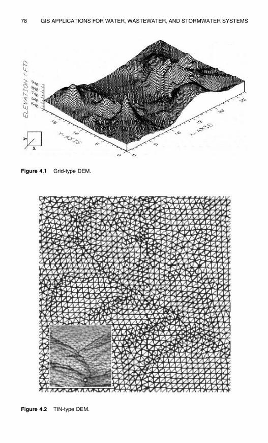
78 GIS APPLICATIONS FOR WATER, WASTEWATER, AND STORMWATER SYSTEMS
Figure 4.1 Grid-type DEM.
Figure 4.2 TIN-type DEM.

DEM APPLICATIONS 79
DEM APPLICATIONS
Major DEM applications include (USGS, 2000):
• Delineating watershed boundaries and streams• Developing parameters for hydrologic models• Modeling terrain gravity data for use in locating energy resources• Determining the volume of proposed reservoirs• Calculating the amount of material removed during strip mining• Determining landslide probability
Jenson and Dominique (1988) demonstrated that drainage characteristics couldbe defined from a DEM. DEMs can be used for automatic delineation of watershedand sewershed boundaries. DEM data can be processed to calculate various water-shed and sewershed characteristics that are used for H&H modeling of watershedsand sewersheds. DEMs can create shaded relief maps that can be used as base mapsin a GIS for overlaying vector layers such as water and sewer lines. DEM files maybe used in the generation of graphics such as isometric projections displaying slope,direction of slope (aspect), and terrain profiles between designated points. This aspectidentifies the steepest downslope direction from each cell to its neighbors.
Raster GIS software packages can convert the DEMs into image maps for visualdisplay as layers in a GIS. DEMs can be used as source data for digital orthophotos.They can be used to create digital orthophotos by orthorectification of aerial photos,as described in Chapter 3 (Remote Sensing Applications). DEMs can also serve astools for many activities including volumetric analysis and site location of towers.DEM data may also be combined with other data types such as stream locations andweather data to assist in forest fire control, or they may be combined with remotesensing data to aid in the classification of vegetation.
Three-Dimensional (3D) Visualization
Over the past decade, 3D computer modeling has evolved in most of the engi-neering disciplines including, but not limited to, layout, design, and construction ofindustrial and commercial facilities; landscaping; highway, bridge, and embankmentdesign; geotechnical engineering; earthquake analysis; site planning; hazardous-wastemanagement; and digital terrain modeling. The 3D visualization can be used forlandscape visualizing or fly-through animation movies of the project area. 3D anima-tions are highly effective tools for public- and town-meeting presentations. GIS canbe used to create accurate topographic elevation models and generate precise 3D data.A DEM is a powerful tool and is usually as close as most GISs get to 3D modeling.
3D graphics are commonly used as a visual communication tool to display a3D view of an object on two-dimensional (2D) media (e.g., a paper map). Untilthe early 1980s, a large mainframe computer was needed to view, analyze, andprint objects in 3D graphics format. Hardware and software are now available for3D modeling of terrain and utility networks on personal computers. Although DEMsare raster images, they can be imported into 3D visualizations packages. Affordableand user-friendly software tools are bringing more users into the world of GIS.

80 GIS APPLICATIONS FOR WATER, WASTEWATER, AND STORMWATER SYSTEMS
These software tools and 3D data can be used to create accurate virtual realityrepresentations of landscape and infrastructure with the help of stereo imagery andautomatic extraction of 3D information. For example, Skyline Software System’s(www.skylinesoft.com) TerraExplorer provides realistic, interactive, photo-based3D maps of many locations and cities of the world on the Internet.
Satellite imagery is also driving new 3D GIS applications. GIS can be used toprecisely identify a geographic location in 3D space and link that location and itsattributes through the integration of photogrammetry, remote sensing, GIS, and 3Dvisualization. 3D geographic imaging is being used to create orthorectified imagery,DEMs, stereo models, and 3D features.
DEM RESOLUTION AND ACCURACY
The accuracy of a DEM is dependent upon its source and the spatial resolution(grid spacing). DEMs are classified by the method with which they were preparedand the corresponding accuracy standard. Accuracy is measured as the root meansquare error (RMSE) of linearly interpolated elevations from the DEM, comparedwith known elevations. According to RMSE classification, there are three levels ofDEM accuracy (Walski et al., 2001):
• Level 1: Based on high-altitude photography, these DEMs have the lowest accu-racy. The vertical RMSE is 7 m and the maximum permitted RMSE is 15 m.
• Level 2: These are based on hypsographic and hydrographic digitization, followedby editing to remove obvious errors. These DEMs have medium accuracy. Themaximum permitted RMSE is one half of the contour interval.
• Level 3: These are based on USGS digital line graph (DLGs) data (Shamsi, 2002).The maximum permitted RMSE is one third of the contour interval.
The vertical accuracy of 7.5-min DEMs is greater than or equal to 15 m. Thus,the 7.5-min DEMs are suitable for projects at 1:24,000 scale or smaller (Zimmer,2001a). A minimum of 28 test points per DEM are required (20 interior points and8 edge points). The accuracy of the 7.5-min DEM data, together with the dataspacing, adequately support computer applications that analyze hypsographic fea-tures to a level of detail similar to manual interpretations of information as printedat map scales not larger than 1:24,000. Early DEMs derived from USGS quadranglessuffered from mismatches at boundaries (Lanfear, 2000).
DEM selection for a particular application is generally driven by data availability,judgment, experience, and test applications (ASCE, 1999). For example, becauseno firm guidelines are available for selection of DEM characteristics for hydrologicmodeling, a hydrologic model might need 30-m resolution DEM data but mighthave to be run with 100-m data if that is the best available data for the study area.In the U.S., regional-scale models have been developed at scales of 1:250,000 to1:2,000,000 (Laurent et al., 1998). Seybert (1996) concluded that modeled watershedrunoff peak flow values are more sensitive to changes in spatial resolution thanmodeled runoff volumes. An overall subbasin area to grid–cell area ratio of 102 wasfound to produce reasonable model results.

DEM APPLICATIONS 81
The grid size and time resolution used for developing distributed hydrologicmodels for large watersheds is a compromise between the required accuracy, availabledata accuracy, and computer run-time. Finer grid size requires more computing time,more extensive data, and more detailed boundary conditions. Chang et al. (2000)conducted numerical experiments to determine an adequate grid size for modelinglarge watersheds in Taiwan where 40 m
× 40 m resolution DEM data are available.They investigated the effect of grid size on the relative error of peak discharge andcomputing time. Simulated outlet hydrographs showed higher peak discharge as thecomputational grid size was increased. In a study, for a watershed of 526 km2 locatedin Taiwan, a grid resolution of 200 m
× 200 m was determined to be adequate.Table 4.1 shows suggested DEM resolutions for various applications (Maidment,
1998). Large (30-m) DEMs are recommended for water distribution modeling (Wal-ski et al., 2001).
The size of a DEM file depends on the DEM resolution, i.e., the finer the DEMresolution, the smaller the grid, and the larger the DEM file. For example, if thegrid size is reduced by one third, the file size will increase nine times. Plotting andanalysis of high-resolution DEM files are slower because of their large file sizes.
USGS DEMS
In the U.S., the USGS provides DEM data for the entire country as part of theNational Mapping Program. The National Mapping Division of USGS has scannedall its paper maps into digital files, and all 1:24,000-scale quadrangle maps nowhave DEMs (Limp, 2001).
USGS DEMs are the (x,y,z) triplets of terrain elevations at the grid nodes of theUniversal Transverse Mercator (UTM) coordinate system referenced to the NorthAmerican Datum of 1927 (NAD27) or 1983 (NAD83) (Shamsi, 1991). USGS DEMsprovide distance in meters, and elevation values are given in meters or feet relativeto the National Geodetic Vertical Datum (NGVD) of 1929. The USGS DEMs areavailable in 7.5-min, 15-min, 2-arc-sec (also known as 30-min), and 1˚ units. The7.5- and 15-min DEMs are included in the large-scale category, whereas 2-arc-secDEMs fall within the intermediate-scale category and 1˚ DEMs fall within the small-scale category. Table 4.2 summarizes the USGS DEM data types.
This chapter is mostly based on applications of 7.5-min USGS DEMs. TheDEM data for 7.5-min units correspond to the USGS 1:24,000-scale topographicquadrangle map series for all of the U.S. and its territories. Thus, each 7.5-min
Table 4.1 DEM Applications
DEMResolution
ApproximateCell Size
WatershedArea (km2)
TypicalApplication
1 sec 30 m 5 Urban watersheds 3 sec 100 m 40 Rural watersheds15 sec 500 m 1,000 River basins, States30 sec 1 km 4,000 Nations 3 min 5 km 150,000 Continents 5 min 10 km 400,000 World

82 GIS APPLICATIONS FOR WATER, WASTEWATER, AND STORMWATER SYSTEMS
by 7.5-min block provides the same coverage as the standard USGS 7.5-min mapseries. Each 7.5-min DEM is based on 30-m by 30-m data spacing; therefore, theraster grid for the 7.5-min USGS quads are 30 m by 30 m. That is, each 900 m2
of land surface is represented by a single elevation value. USGS is now movingtoward acquisition of 10-m accuracy (Murphy, 2000).
USGS DEM Formats
USGS DEMs are available in two formats:
1. DEM file format: This older file format stores DEM data as ASCII text, as shownin Figure 4.3. These files have a file extension of dem (e.g., lewisburg_PA.dem).These files have three types of records (Walski et al., 2001):• Type A: This record contains information about the DEM, including name,
boundaries, and units of measurements.
Table 4.2 USGS DEM Data Formats
DEM Type Scale Block Size Grid Spacing
Large 1:24,000 7.5 ft
× 7.5 ft 30 mIntermediate Between large and small 30 ft
× 30 ft 2 secSmall 1:250,000 1
°
× 1
° 3 sec
Figure 4.3 USGS DEM file.

DEM APPLICATIONS 83
• Type B: These records contain elevation data arranged in “profiles” from southto north, with the profiles organized from west to east. There is one Type-Brecord for each south–north profile.
• Type C: This record contains statistical information on the accuracy of DEM.2. Spatial Data Transfer Standard (SDTS): This is the latest DEM file format that
has compressed data for faster downloads. SDTS is a robust way of transferringgeoreferenced spatial data between dissimilar computer systems and has the poten-tial for transfer with no information loss. It is a transfer standard that embracesthe philosophy of self-contained transfers, i.e., spatial data, attribute, georeferenc-ing, data quality report, data dictionary, and other supporting metadata; all areincluded in the transfer. SDTS DEM data are available as tar.gz compressed files.Each compressed file contains 18 ddf files and two readme text files. For furtheranalysis, the compressed SDTS files should be unzipped (uncompressed). Stan-dard zip programs, such as PKZIP, can be used for this purpose.
Some DEM analysis software may not read the new SDTS data. For suchprograms, the user should translate the SDTS data to a DEM file format. SDTStranslator utilities, like SDTS2DEM or MicroDEM, are available from the GeoCom-munity’s SDTS Web site to convert the SDTS data to other file formats.
National Elevation Dataset (NED)
Early DEMs were derived from USGS quadrangles, and mismatches at bound-aries continued to plague the use of derived drainage networks for larger areas(Lanfear, 2000). The NED produced by USGS in 1999 is the new generation ofseamless DEM that largely eliminates problems of quadrangle boundaries and otherartifacts. Users can now select DEM data for their area of interest.
The NED has been developed by merging the highest resolution, best-qualityelevation data available across the U.S. into a seamless raster format. NED is designedto provide the U.S. with elevation data in a seamless form, with a consistent datum,elevation unit, and projection. Data corrections were made in the NED assemblyprocess to minimize artifacts, perform edge matching, and fill sliver areas of missingdata. NED is the result of the maturation of the USGS effort to provide 1:24,000-scale DEM data for the conterminous U.S. and 1:63,360-scale DEM data for Alaska.NED has a resolution of 1 arc-sec (approximately 30 m) for the conterminous U.S.,Hawaii, and Puerto Rico and a resolution of 2 arc-sec for Alaska. Using a hill-shadetechnique, USGS has also derived a shaded relief coverage that can be used as a basemap for vector themes. Other themes, such as land use or land cover, can be drapedon the NED-shaded relief maps to enhance the topographic display of themes. TheNED store offers seamless data for sale, by user-defined area, in a variety of formats.
DEM DATA AVAILABILITY
USGS DEMs can be downloaded for free from the USGS geographic datadownload Web site. DEM data on CD-ROM can also be purchased from the USGSEarthExplorer Web site for an entire county or state for a small fee to cover theshipping and handling cost. DEM data for other parts of the world are also available.
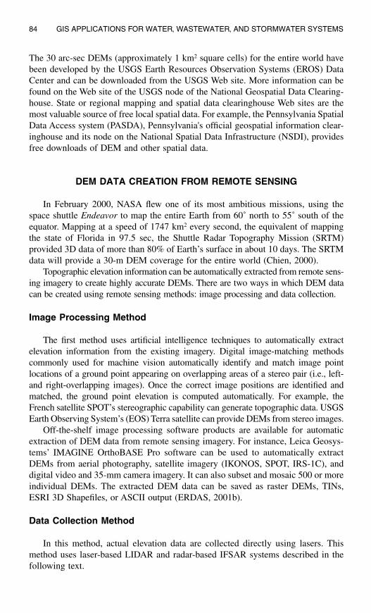
84 GIS APPLICATIONS FOR WATER, WASTEWATER, AND STORMWATER SYSTEMS
The 30 arc-sec DEMs (approximately 1 km2 square cells) for the entire world havebeen developed by the USGS Earth Resources Observation Systems (EROS) DataCenter and can be downloaded from the USGS Web site. More information can befound on the Web site of the USGS node of the National Geospatial Data Clearing-house. State or regional mapping and spatial data clearinghouse Web sites are themost valuable source of free local spatial data. For example, the Pennsylvania SpatialData Access system (PASDA), Pennsylvania's official geospatial information clear-inghouse and its node on the National Spatial Data Infrastructure (NSDI), providesfree downloads of DEM and other spatial data.
DEM DATA CREATION FROM REMOTE SENSING
In February 2000, NASA flew one of its most ambitious missions, using thespace shuttle Endeavor to map the entire Earth from 60˚ north to 55˚ south of theequator. Mapping at a speed of 1747 km2 every second, the equivalent of mappingthe state of Florida in 97.5 sec, the Shuttle Radar Topography Mission (SRTM)provided 3D data of more than 80% of Earth’s surface in about 10 days. The SRTMdata will provide a 30-m DEM coverage for the entire world (Chien, 2000).
Topographic elevation information can be automatically extracted from remote sens-ing imagery to create highly accurate DEMs. There are two ways in which DEM datacan be created using remote sensing methods: image processing and data collection.
Image Processing Method
The first method uses artificial intelligence techniques to automatically extractelevation information from the existing imagery. Digital image-matching methodscommonly used for machine vision automatically identify and match image pointlocations of a ground point appearing on overlapping areas of a stereo pair (i.e., left-and right-overlapping images). Once the correct image positions are identified andmatched, the ground point elevation is computed automatically. For example, theFrench satellite SPOT’s stereographic capability can generate topographic data. USGSEarth Observing System’s (EOS) Terra satellite can provide DEMs from stereo images.
Off-the-shelf image processing software products are available for automaticextraction of DEM data from remote sensing imagery. For instance, Leica Geosys-tems’ IMAGINE OrthoBASE Pro software can be used to automatically extractDEMs from aerial photography, satellite imagery (IKONOS, SPOT, IRS-1C), anddigital video and 35-mm camera imagery. It can also subset and mosaic 500 or moreindividual DEMs. The extracted DEM data can be saved as raster DEMs, TINs,ESRI 3D Shapefiles, or ASCII output (ERDAS, 2001b).
Data Collection Method
In this method, actual elevation data are collected directly using lasers. Thismethod uses laser-based LIDAR and radar-based IFSAR systems described in thefollowing text.

DEM APPLICATIONS 85
LIDAR
Unlike photogrammetric techniques, which can be time consuming and expensivefor large areas, this method is a cost-effective alternative to conventional technologies.It can create DEMs with accuracy levels ranging from 20 to 100 cm, which aresuitable for many engineering applications. This remote-sensing technology does noteven involve an image. Laser imaging detection and ranging (LIDAR) is a new systemfor measuring ground surface elevation from an airplane. LIDAR can collect 3Ddigital data on the fly. LIDAR sensors provide some of the most accurate elevationdata in the shortest time ever by bouncing laser beams off the ground. LIDARtechnology, developed in the mid-1990s, combines global positioning system (GPS),precision aircraft guidance, laser range finding, and high-speed computer processingto collect ground elevation data. Mounted on an aircraft, a high-accuracy scannersweeps the laser pulses across the flight path and collects reflected light. A laserrange-finder measures the time between sending and receiving each laser pulse todetermine the ground elevation below. The LIDAR system can survey up to 10,000acres per day and provide horizontal and vertical accuracies up to 12 and 6 in.,respectively. Chatham County, home of Savannah, Georgia, used the LIDAR approachto collect 1-ft interval contour data for the entire 250,000 acre county in less than ayear. The cost of conventional topographic survey for this data would be over $20million. The County saved $7 million in construction cost by using data from AirborneLaser Terrain Mapping (ALTM) technology, a LIDAR system manufactured byOptech, Canada. The new ALTM data were used to develop an accurate hydraulicmodel of the Hardin basin (Stones, 1999).
Chatham County, Georgia, saved $7 million in construction cost by using LIDAR data.
Boise-based Idaho Power Company spent $273,000 on LIDAR data for a 290km stretch of the rugged Hell’s Canyon, through which the Snake River runs. Thecost of LIDAR data was found to be less than aerial data and expensive ground-surveying. The company used LIDAR data to define the channel geometry, combinedit with bathymetry data, and created digital terrain files containing ten cross sectionsof the canyon per mile. The cross-section data were input to a hydraulic model thatdetermined the effect of power plants’ releases on vegetation and wildlife habitats(Miotto, 2000).
IFSAR
Interferometric Synthetic Aperture Radar (IFSAR) is an aircraft-mounted radarsystem for quick and accurate mapping of large areas in most weather conditionswithout ground control. Because it is an airborne radar, IFSAR collects elevationdata on the first try in any weather (regardless of fog, clouds, or rain), day or night,significantly below the cost of satellite-derived DEM. The IFSAR process measureselevation data at a much denser grid than photogrammetric techniques, using over-lapping stereo images. A denser DEM provides a more detailed terrain surface in

86 GIS APPLICATIONS FOR WATER, WASTEWATER, AND STORMWATER SYSTEMS
an image. IFSAR is efficient because it derives the DEM data by digital processingof a single radar image. This allows elevation product delivery within days of datacollection. A DEM with a minimum vertical accuracy of 2 m is necessary to achievethe precision level orthorectification for IKONOS imagery. DEMs generated fromthe IFSAR data have been found to have the adequate vertical accuracy to orthorec-tify IKONOS imagery to the precision level (Corbley, 2001).
Intermap Technologies’ (Englewood, Colorado, www.intermaptechnologies.com) Lear jet-mounted STAR-3i system, an airborne mapping system, has beenreported to provide simultaneous high-accuracy DEMs and high-resolution orthorec-tified imagery without ground control. STAR-3i IFSAR system typically acquireselevation points at 5-m intervals, whereas photogrammetric sources use a spacing of30 to 50 m. STAR-3i can provide DEMs with a vertical accuracy of 30 cm to 3 mand an orthoimage resolution of 2.5 m.
DEM ANALYSIS
Cell Threshold for Defining Streams
Before starting DEM analysis, users must define the minimum number ofupstream cells contributing flow into a cell to classify that cell as the origin of astream. This number, referred to as the cell “threshold,” defines the minimumupstream drainage area necessary to start and maintain a stream. For example, if astream definition value of ten cells is specified, then for a single grid location of theDEM to be in a stream, it must drain at least ten cells. It is assumed that there isflow in a stream if its upstream area exceeds the critical threshold value. In this case,the cell is considered to be a part of the stream. The threshold value can be estimatedfrom existing topographic maps or from the hydrographic layer of the real streamnetwork. Selection of an appropriate cell threshold size requires some user judgment.Users may start the analysis with an assumed or estimated value and adjust the initialvalue by comparing the delineation results with existing topographic maps or hydro-graphic layers. The cell threshold value directly affects the number of subbasins(subwatersheds or subareas). A smaller threshold results in smaller subbasin size,larger number of subbasins, and slower computation speed for the DEM analysis.
The D-8 Model
The 8-direction pour point model, also known as the D-8 model, is a commonlyused algorithm for delineating a stream network from DEMs. As shown in Figure 4.4,it identifies the steepest downslope flow path between each cell and its eight neigh-boring cells. This path is the only flow path leaving the cell. Watershed area isaccumulated downslope along the flow paths connecting adjacent cells. The drainagenetwork is identified from the user-specified threshold area at the bottom of whicha source channel originates and classifies all cells with a greater watershed area aspart of the drainage network. Figure 4.4 shows stream delineation steps using theD-8 model with a cell threshold value of ten cells. Grid A shows the cell elevation

DEM APPLICATIONS 87
values. Grid B shows flow direction arrows based on calculated cell slopes. Grid Cshows the number of accumulated upstream cells draining to each cell. Grid D showsthe delineated stream segment based on the cells with flow accumulation valuesgreater than or equal to ten.
DEM Sinks
The D-8 and many other models do not work well in the presence of depressions,sinks, and flat areas. Some sinks are caused by the actual conditions, such as theGreat Salt Lake in Utah where no watershed precipitation travels through a rivernetwork toward the ocean. The sinks are most often caused by data noise and errorsin elevation data. The computation problems arise because cells in depressions, sinks,and flat areas do not have any neighboring cells at a lower elevation. Under theseconditions, the flow might accumulate in a cell and the resulting flow network maynot necessarily extend to the edge of the grid. Unwanted sinks must be removedprior to starting the stream or watershed delineation process by raising the elevationof the cells within the sink to the elevation of its lowest outlet. Most raster GISsoftware programs provide a FILL function for this purpose. For example, ArcInfo’sGRID extension provides a FILL function that raises the elevation of the sink cellsuntil the water is able to flow out of it.
The FILL approach assumes that all sinks are caused by underestimated elevationvalues. However, the sinks can also be created by overestimated elevation values,in which case breaching of the obstruction is more appropriate than filling the sinkcreated by the obstruction. Obstruction breaching is particularly effective in flat orlow-relief areas (ASCE, 1999).
Figure 4.4 Figure 11-4. D-8 Model for DEM-based stream delineation (A) DEM elevation grid,(B) flow direction grid, (C) flow accumulation grid, and (D) delineated streams forcell threshold of ten.

88 GIS APPLICATIONS FOR WATER, WASTEWATER, AND STORMWATER SYSTEMS
Stream Burning
DEM-based stream or watershed delineations may not be accurate in flat areasor if the DEM resolution failed to capture important topographic information. Thisproblem can be solved by “burning in” the streams using known stream locationsfrom the existing stream layers. This process modifies the DEM grid so that the flowof water is forced into the known stream locations. The cell elevations are artificiallylowered along the known stream locations or the entire DEM is raised except alongknown stream paths. The phrase burning in indicates that the streams have beenforced, or “burned” into the DEM topography (Maidment, 2000). This method mustbe used with caution because it may produce flow paths that are not consistent withthe digital topography (ASCE, 1999).
DEM Aggregation
Distributed hydrologic models based on high-resolution DEMs may requireextensive computational and memory resources that may not be available. In thiscase, high-resolution DEMs can be aggregated into low-resolution DEMs. For exam-ple, it was found that the 30-m USGS DEM would create 80,000 cells for the72.6 km2 Goodwater Creek watershed located in central Missouri. Distributed mod-eling of 80,000 cells was considered time consuming and impractical (Wang et al.,2000). The 30 m
× 30 m cells were, therefore, aggregated into 150 m x 150 m(2.25 ha) cells. In other words, 25 smaller cells were aggregated into one large cell,which reduced the number of cells from 80,000 to approximately 3,000. Best of all,the aggregated DEM produced the same drainage network as the original DEM. Theaggregation method computes the flow directions of the coarse-resolution cells basedon the flow paths defined by the fine-resolution cells. It uses three steps: (1) determinethe flow direction of the fine-resolution DEM, (2) determine outlets of coarse-resolution DEM, and (3) approximate the flow direction of coarse-resolution DEM,based on the flow direction of the fine-resolution DEM.
Slope Calculations
Subbasin slope is an input parameter in many hydrologic models. Most rasterGIS packages provide a SLOPE function for estimating slope from a DEM. Forexample, ERDAS IMAGINE software uses its SLOPE function to compute percentslope by fitting a plane to a pixel elevation and its eight neighboring pixel elevations.The difference in elevation between the low and the high points is divided by thehorizontal distance and multiplied by 100 to compute percent slope for the pixel.Pixel slope values are averaged to compute the mean percent slope of each subbasin.
SOFTWARE TOOLS
The DEM analysis functions described in the preceding subsections requireappropriate software. Representative DEM analysis software tools and utilities arelisted in Table 4.3.

DE
M A
PP
LICA
TIO
NS
89Table 4.3 Sample DEM Analysis Software Tools
Software Vendor and Web site Notes
Spatial Analystand Hydro extension
ESRI, Redlands, California www.esri.com
ArcGIS 8.x and ArcView3.x extension
ARC GRID extension ArcInfo 7.x extension
Analyst ArcGIS 8.x
and ArcView 3.x
extension
IDRISI Clark University Worcester, Massachusettswww.clarklabs.org
ERDAS IMAGINE Leica Geosystems, Atlanta, Georgiagis.leica-geosystems.comwww.erdas.com
Formerly, Earth ResourceData Analysis System(ERDAS) software
TOPAZ U.S. Department of Agriculture,Agricultural Research Service, El Reno, Oklahomagrl.ars.usda.gov/topaz/TOPAZ1.HTM
MicroDEM U.S. Naval Academywww.usna.edu/Users/oceano/pguth/website/microdem.htm
Software developed byPeter Guth of theOceanography Department
DEM3D viewer USGS, Western Mapping Center, Menlo Park, Californiacraterlake.wr.usgs.gov/dem3d.html
Free download, allowsviewing of DEM files througha 3D perspective

90 GIS APPLICATIONS FOR WATER, WASTEWATER, AND STORMWATER SYSTEMS
Some programs such as Spatial Analyst provide both the DEM analysis andhydrologic modeling capabilities. ASCE (1999) has compiled a review of hydrologicmodeling systems that use DEMs. Major DEM software programs are discussed inthe following text.
Spatial Analyst and Hydro Extension
Spatial Analyst is an optional extension (separately purchased add-on program)for ESRI’s ArcView 3.x and ArcGIS 8.x software packages. The Spatial AnalystExtension adds raster GIS capability to the ArcView and ArcGIS vector GIS soft-ware. Spatial Analyst allows for use of raster and vector data in an integratedenvironment and enables desktop GIS users to create, query, and analyze cell-basedraster maps; derive new information from existing data; query information acrossmultiple data layers; and integrate cell-based raster data with the traditional vectordata sources. It can be used for slope and aspect mapping and for several otherhydrologic analyses, such as delineating watershed boundaries, modeling streamflow, and investigating accumulation. Spatial Analyst for ArcView 3.x has most, butnot all, of the functionality of the ARC GRID extension for ArcInfo 7.x softwarepackage described below.
Spatial Analyst for ArcView 3.x is supplied with a Hydro (or hydrology) exten-sion that further extends the Spatial Analyst user interface for creating input datafor hydrologic models. This extension provides functionality to create watershedsand stream networks from a DEM, calculate physical and geometric properties ofthe watersheds, and aggregate these properties into a single-attribute table that canbe attached to a grid or Shapefile. Hydro extension requires that Spatial Analyst bealready installed. Hydro automatically loads the Spatial Analyst if it is not loaded.
Depending upon the user needs, there are two approaches to using the Hydroextension:
1. Hydro pull-down menu options: If users only want to create watershed subbasinsor the stream network, they should work directly with the Hydro pull-downmenu options (Figure 4.5). Table 4.4 provides a brief description of each ofthese menu options. “Fill Sinks” works off an active elevation grid theme. “FlowDirection” works off an active elevation grid theme that has been filled. “FlowAccumulation” works off an active flow direction grid theme. “Flow Length”works off an active flow direction grid theme. “Watershed” works off an activeflow accumulation grid theme and finds all basins in the data set based on aminimum number of cells in each basin. The following steps should be performedto create watersheds using the Hydro pull-down menu options, with the outputgrid from each step serving as the input grid for the next step:• Import the raw USGS DEM.• Fill the sinks using the “Fill Sinks” menu option (input = raw USGS DEM).
This is a very important intermediate step. Though some sinks are valid, mostare data errors and should be filled.
• Compute flow directions using the “Flow Direction” menu option (input =filled DEM grid).
• Compute flow accumulation using the “Flow Accumulation” menu option(input = flow directions grid).

DEM APPLICATIONS 91
• Delineate streams using the “Stream Network” menu option (input = flowaccumulation grid).
• Delineate watersheds using the “Watershed” menu option.2. Hydrologic Modeling Dialogue: If users want to create subbasins and calculate many
additional attributes for them, they should use the Hydrologic Modeling Dialogue(Figure 4.6), which is the first choice under the Hydro pull-down menu. The Hydro-logic Modeling Dialogue is designed to be a quick one-step method for calculatingand then aggregating a set of watershed attributes to a single file. This file can thenbe used in a hydrologic model, such as the Watershed Modeling System (WMS)(discussed in Chapter 11 [Modeling Applications]), or it can be reformatted for inputinto HEC’s HMS model, or others. The following steps should be performed tocreate watersheds using the Hydrologic Modeling Dialogue:• Choose “Delineate” from DEM and select an elevation surface.• Fill the sinks when prompted.• Specify the cell threshold value when prompted. This will create watersheds
based on the number of cells or up-slope area defined by the user as the smallestwatershed wanted.
Additional DEM analysis resources (tutorials, exercises, sample data, softwareutilities, reports, papers, etc.) are provided at the following Web sites:
• ESRI Web site at www.esri.com/arcuser/ (do a search for “Terrain Modeling”)• University of Texas at Austin (Center for Research in Water Resources) Web site
at www.crwr.utexas.edu/archive.shtml
The last four Hydro options (Table 4.4) work with existing data layers. They donot create elevation, slope, precipitation, and runoff curve number layers. They
Figure 4.5 Hydro extension pull-down menu.

92 GIS APPLICATIONS FOR WATER, WASTEWATER, AND STORMWATER SYSTEMS
simply compute mean areal values of these four parameters for the subbasins, usingthe existing GIS layers of these parameters. Thus, the GIS layers of elevation, slope,precipitation, and runoff curve number must be available to use the mean functionsof the Hydro extension.
Figure 4.7 shows Hydro’s raindrop or pour point feature. Using this capability,the user can trace the flow path from a specified point to the watershed outlet. Hydroalso calculates a flow length as the maximum distance along the flow path withineach watershed. The flow path can be divided by the measured or estimated velocityto estimate the time of concentration or travel time that are used to estimate runoffhydrographs. Travel time can also be used to estimate the time taken by a hazardouswaste spill to reach a sensitive area or water body of the watershed. Laurent et al.(1998) used this approach to estimate travel time between any point of a watershedand a water resource (river or well). This information was further used to create amap of water resources vulnerability to dissolved pollution in an area in MassifCentral, France. Subbasin area can be divided by flow length to estimate the overlandflow width for input to a rainfall-runoff model such as EPA’s Storm Water Manage-ment Model (SWMM).
Table 4.4 Hydro Extension Menu Options
Hydro Menu Option Function
Hydrologic modeling Creates watersheds and calculates their attributesFlow direction Computes the direction of flow for each cell in a DEMIdentify sinks Creates a grid showing the location of sinks or areas of
internal drainage in a DEMFill sinks Fills the sinks in a DEM, creating a new DEMFlow accumulation Calculates the accumulated flow or number of up-slope
cells, based on a flow direction gridWatershed Creates watersheds based upon a user-specified flow
accumulation thresholdArea Calculates the area of each watershed in a watershed
gridPerimeter Calculates the perimeter of each watershed in a
watershed gridLength Calculates the straight-line distance from the pour
point to the furthest perimeter point for each watershedFlow length Calculates the length of flow path for each cell
to the pour point for each watershedFlow length by watershed Calculates the maximum distance along the flow path
within each watershedShape factor by watershed Calculates a shape factor (watershed length squared
and then divided by watershed area) for each watershedStream network as line shape Creates a vector stream network from a flow
accumulation grid, based on a user-specified thresholdCentroid as point shape Creates a point shape file of watershed centroidsPour points as point shape Creates a point shape file of watershed pour pointsMean elevation Calculates the mean elevation within each watershedMean slope Calculates the mean slope within each watershedMean precipitation Calculates the mean precipitation in each watershedMean curve number Calculates the mean curve number for each watershed

DEM APPLICATIONS 93
ARC GRID Extension
ARC GRID is an optional extension for ESRI’s ArcInfo
7.x GIS softwarepackage. GRID adds raster geoprocessing and hydrologic modeling capability to thevector-based ArcInfo GIS. For hydrologic modeling, the extension offers a Hydro-logic Tool System and several hydrologically relevant functions for watershed andstream network delineation.
The FLOWDIRECTION function creates a grid of flow directions from eachcell to the steepest downslope neighbor. The results of FLOWDIRECTION are usedin many subsequent functions such as stream delineation. The FLOWACCUMULA-TION function calculates upstream area or cell-weighted flow draining into eachcell. The WATERSHED function delineates upstream tributary area at any user-specified point, channel junction, or basin outlet cell. This function requires step-by-step calculations. Arc Macro Language (AML) programs can be written to auto-mate this function for delineating subbasins at all the stream nodes.
GRID can find upstream or downstream flow paths from any cell and determinetheir lengths. GRID can perform stream ordering and assign unique identifiers tothe links of a stream network delineated by GRID. Spatial intersection betweenstreams and subbasins can define the links between the subbasins and streams. Thismethod relates areal attributes such as subbasin nutrient load to linear objects suchas streams. The NETWORK function can then compute the upstream accumulatednutrient load for each stream reach (Payraudeau et al., 2000). This approach is alsouseful in DEM-based runoff quality modeling.
Figure 4.6 Hydro extension Hydrologic Modeling Dialogue.

94 GIS APPLICATIONS FOR WATER, WASTEWATER, AND STORMWATER SYSTEMS
IDRISI
IDRISI is not an acronym; it is named after a cartographer born in 1099 A.D.in Morocco, North Africa. IDRISI was developed by the Graduate School of Geog-raphy at Clark University. IDRISI provides GIS and remote sensing software func-tions, from database query through spatial modeling to image enhancement andclassification. Special facilities are included for environmental monitoring and nat-ural resource management, including change and time-series analysis, multicriteriaand multiobjective decision support, uncertainty analysis (including Bayesian andFuzzy Set analysis), and simulation modeling (including force modeling and aniso-tropic friction analysis). TIN interpolation, Kriging, and conditional simulation arealso offered.
IDRISI is basically a raster GIS. IDRISI includes tools for manipulating DEMdata to extract streams and watershed boundaries. IDRISI GIS data has an openformat and can be manipulated by external computer programs written by users.This capability makes IDRISI a suitable tool for developing hydrologic modelingapplications. For example, Quimpo and Al-Medeij (1998) developed a FORTRAN
Figure 4.7 Hydro extension’s pour point feature.

DEM APPLICATIONS 95
program to model surface runoff using IDRISI. Their approach consisted of delin-eating watershed subbasins from DEM data and estimating subbasin runoff curvenumbers from soils and land-use data.
Figure 4.8 shows IDRISI’s DEM analysis capabilities. The upper-left windowshows a TIN model created from digital contour data. The upper-right window showsa DEM created from the TIN with original contours overlayed. The lower-rightwindow shows an illuminated DEM emphasizing relief. The lower-left windowshows a false color composite image (Landsat TM bands 2, 3, and 4) draped overthe DEM (IDRISI, 2000).
TOPAZ
TOPAZ is a software system for automated analysis of landscape topographyfrom DEMs (Topaz, 2000). The primary objective of TOPAZ is the systematicidentification and quantification of topographic features in support of investigationsrelated to land-surface processes, H&H modeling, assessment of land resources,and management of watersheds and ecosystems. Typical examples of topographicfeatures that are evaluated by TOPAZ include terrain slope and aspect, drainagepatterns and divides, channel network, watershed segmentation, subcatchmentidentification, geometric and topologic properties of channel links, drainage dis-tances, representative subcatchment properties, and channel network analysis(Garbrecht and Martz, 2000). The FILL Function of TOPAZ recognizes depressionscreated by embankments and provides outlets for these without filling, a betterapproach than the fill-only approach in other programs (e.g., IDRISI or SpatialAnalyst).
CASE STUDIES AND EXAMPLES
Representative applications of using DEM data in GIS are described in thissection.
Watershed Delineation
A concern with streams extracted from DEMs is the precise location of streams.Comparisons with actual maps or aerial photos often show discrepancies, especiallyin low-relief landscapes (ASCE, 1999). A drainage network obtained from a DEMmust be comparable to the actual hydrologic network. Thus, it is worthwhile tocheck the accuracy of DEM-based delineations. This can be done by comparing theDEM delineations with manual delineations. Jenson (1991) found approximately97% similarity between automatic and manual delineations from 1:50,000-scaletopographic maps.
The objective of this case study was to test the efficacy of DEM-based automaticdelineation of watershed subbasins and streams. It was assumed that manual delin-eations are more accurate than DEM delineations. Thus, a comparison of manualand DEM delineations was made to test the accuracy of DEM delineations.

96G
IS A
PP
LICA
TIO
NS
FO
R W
AT
ER
, WA
ST
EW
AT
ER
, AN
D S
TO
RM
WA
TE
R S
YS
TE
MS
Figure 4.8 IDRISI’s DEM analysis features.

DEM APPLICATIONS 97
The case study watershed is the Bull Run Watershed located in Union Countyin north-central Pennsylvania (Shamsi, 1996). This watershed was selected becauseof its small size so that readable report-size GIS maps can be printed. The proposedtechnique has also been successfully applied to large watersheds with areas of severalhundred square miles. Bull Run Watershed’s 8.4 mi2 (21.8 km2) drainage area istributary to the West Branch Susquehanna River at the eastern boundary of LewisburgBorough. The 7.5-min USGS topographic map of the watershed is shown inFigure 4.9. The predominant land use in the watershed is open space and agricultural.Only 20% of the watershed has residential, commercial, and industrial land uses.
Manual watershed subdivision was the first step of the case study. The 7.5-minUSGS topographic map of the study area was used for manual subbasin delineation,which resulted in the 28 subbasins shown in Figure 4.9. This figure also shows themanually delineated streams (dashed lines).
Next, ArcView Spatial Analyst and Hydro extension were used to delineatesubbasins and streams using the 7.5-min USGS DEM data. Many cell threshold values(50, 100, 150, …, 1000) were used repeatedly to determine which DEM delineationsagreed with manual delineations. Figure 4.10, Figure 4.11, and Figure 4.12 show theDEM subbasins for cell thresholds of 100, 250, and 500. These figures also showthe manual subbasins for comparison. It can be seen that the 100 threshold createstoo many subbasins. The 500 threshold provides the best agreement between manualand DEM delineations.
Figure 4.13, Figure 4.14, and Figure 4.15 show the DEM streams for cellthreshold values of 100, 250, and 500. These figures also show the manually delin-eated streams for comparison purposes. It can be seen that the 100 threshold createstoo many streams (Figure 4.13); the 500 threshold looks best (Figure 4.15) and
Figure 4.9 Bull Run Watershed showing manual subbasins and streams.

98 GIS APPLICATIONS FOR WATER, WASTEWATER, AND STORMWATER SYSTEMS
provides the best agreement between the manual and DEM streams. The upper-rightboundary of the watershed in Figure 4.15 shows that one of the DEM streams crossesthe watershed boundary. This problem is referred to as the boundary “cross-over”problem, which is not resolved by altering threshold values. It must be corrected bymanual editing of DEM subbasins or using DEM preprocessing methods such asthe stream burning method described earlier.
Figure 4.10 Manual vs. DEM subbasins for cell threshold of 100 (too many subbasins).
Figure 4.11 Manual vs. DEM subbasins for cell threshold of 250 (better).

DEM APPLICATIONS 99
Figure 4.16 shows DEM-derived subbasin and stream maps for a portion of thevery large Monongahela River Basin located in south western Pennsylvania, usingthe 30-m USGS DEM data and a cell threshold value of 500 cells.
From the Bull Run watershed case study, it can be concluded that for rural andmoderately hilly watersheds, 30-m resolution DEMs are appropriate for automaticdelineation of watershed subbasins and streams. The 30-m DEMs work well for themountainous watersheds like those located in Pennsylvania where subbasin boundaries
Figure 4.12 Manual vs. DEM subbasins for cell threshold of 500 (best).
Figure 4.13 Manual vs. DEM streams for cell threshold of 100 (too many streams).

100 GIS APPLICATIONS FOR WATER, WASTEWATER, AND STORMWATER SYSTEMS
are well defined and distinct due to highly variable topography. For 30-m USGS DEMs,a cell threshold of 500 is appropriate. Stream networks generated from the 30-m USGSDEMs at a cell threshold value of 500 were satisfactory, with a minor watershedboundary crossover problem. Correction of boundary crossover problems mightrequire some manual intervention to ensure the efficacy of the DEM-based automatic
Figure 4.14 Manual vs. DEM streams for cell threshold of 250 (better).
Figure 4.15 Manual vs. DEM streams for cell threshold of 500 (best).

DEM APPLICATIONS 101
watershed delineation approach. Compared with the manual watershed delineationapproach, the DEM approach offers significant time savings, eliminates user subjec-tivity, and produces consistent results.
Sewershed Delineation
Watersheds define the drainage areas of natural streams and rivers. Sewershedsdefine the drainage areas of man-made sewers and storm drains. The conventionalmanual method of sewershed delineation is cumbersome, and an automated methodis desirable. Can we use DEMs for automatic delineation of sewersheds? Unfortu-nately, the current research indicates that DEMs are generally applicable to naturallandscapes and may not apply to urbanized settings (ASCE, 1999). This limitationis expected to be more pronounced in low-relief or flat areas. DEM delineations arebased on the premise that water flows in the downslope direction, i.e., that all thesewers are gravity pipes. Therefore, DEM-based sewershed delineations will not beaccurate for a pumped system with force mains and will require manual editing ofthe sewershed boundaries.
Figure 4.17 shows a comparison of DEM watersheds (filled polygons) andmanually delineated sewersheds for the gravity sewers area of the Borough ofCharleroi located near Pittsburgh, Pennsylvania. The watersheds were created fromthe 30-m resolution USGS DEM of the study area using a cell threshold of 100.The mean land slope of the study area is approximately 15%. The comparison showsthat some sewersheds (for example, Sewershed Nos. 3, 4, 5, and 6) are reasonably
Figure 4.16 DEM-derived watersheds and streams for a large watershed.

102 GIS APPLICATIONS FOR WATER, WASTEWATER, AND STORMWATER SYSTEMS
close to the watershed boundaries and some sewersheds (for example, SewershedNo. 2) are quite different from the watershed boundaries.
The Massachusetts Water Resources Authority (MWRA) recently determined thatDEMs were not too helpful in delineating sewershed boundaries (Herrlin, 2000).MWRA, instead, used a “Euclidean Distance” approach consisting of the following steps:
1. All the sewers tributary to a pour point (point where a trunk sewer connects aninterceptor) are identified using a custom network-tracing utility (upstream trace).The group of pipes identified like this defines a tributary area.
2. A new attribute with the name of the tributary area is manually added to all thesewers. This step is quite laborious but needs to be done only once.
3. Vector sewer layers are converted to a grid format. This is necessary because theEuclidean distance approach works only on raster layers.
4. The Euclidean distance allocation function is applied to all the sewer cells. TheEuclidean distance is calculated in the same manner as finding the hypotenuse ofa triangle. This generates a sewershed boundary around sewers.
5. The raster Euclidean distance boundaries are converted back to vector (polygon)format.
Figure 4.17 Comparison of DEM watersheds (filled polygons) and manually drawn sewer-sheds.

DEM APPLICATIONS 103
Some techniques that may be used for improving the accuracy of DEM-basedsewershed delineations are listed below:
1. Use large-scale, high-resolution DEMs derived from digital orthophotos. Theserelatively dense DEMs have break lines at breaks in grades, which may providevaluable information for delineating sewersheds in flat urban areas. LIDAR tech-nology can also provide highly accurate and cost-effective DEMs and 3D breaklines that can be used for delineating sewersheds.
2. Burning in the DEMs with streams improves the accuracy of delineated watershedsin flat areas. Burning in the DEMs with sewers may improve the delineatedsewersheds.
3. Adding manhole rim elevations to DEMs may be helpful in delineating sewer-sheds. Alternatively, DEMs may be burned in with manhole rim elevations.
Water Distribution System Modeling
The performance of a water distribution system depends on variations in groundsurface elevation. For example, high-elevation areas may experience inadequatepressure if appropriate pumping is not provided. Thus, all distribution system modelsrequire input data for the elevation of each model node. DEMs can be used for 3Drepresentation of water systems and estimating elevation at the nodes of a waterdistribution network model.
Shamsi (1991) showed applications of personal computer-based 3D graphics innetwork and reliability modeling of water distribution systems. Optional 3D exten-sions of GIS software, such as ESRI’s 3D Analyst, can create 3D maps of terrain,water demand, and modeled pressures. Figure 4.18 shows three stacked surfaces:ground surface elevations, demands, and modeled average daily pressures for theBorough of White Haven, Pennsylvania. The land area of the borough is 773 acres,the population is 1,091 persons, and the average daily demand is 197,000 gal/d. Thedistribution system consists of water mains ranging in size from 2 to 8 in. It isinteresting to note the high-pressure areas coinciding with the low-elevation areas,and vice versa. It also quickly becomes apparent that the high-demand areas pre-dominate in the lower elevations. A display such as Figure 4.18 is an effective visualaid to displaying the hydraulic model results. Most importantly, such graphics canbe easily understood by system operators without the extensive training that isusually required to understand the model output in tabular format.
Node elevation is a critical input parameter for all water distribution systemmodels. Traditionally, the node elevations have been determined manually by over-laying the water distribution network over a topographic map of the study area.Unfortunately, due to its tedious nature, this approach is cumbersome. GIS is nowbeing used to automatically extract the node elevations from a DEM of the studyarea. This approach requires a vector layer of the network nodes, a DEM grid, anda user script. The script appends a new “Elevation” field to the “Node” layer table,queries the DEM grid at node locations, and writes the elevation values in theElevation field.

104 GIS APPLICATIONS FOR WATER, WASTEWATER, AND STORMWATER SYSTEMS
WaterCAD Example
If node locations are available in an ArcView Shapefile, ArcView 3D Analystextension (Version 3.x) can be used to calculate node elevation from a DEM grid.This extension uses bilinear interpolation to calculate the node elevation from the
Figure 4.18 Hydraulic modeling results as 3D surfaces.

DEM APPLICATIONS 105
grid cell elevation data. The elevation data are pulled from the DEM overlay, and thenode file is converted to a 3D file. The steps for this procedure for Haestad Method’sWaterCAD modeling software are listed below (Walski et al., 2001):
1. Start ArcView and load the 3D Analyst extension.2. Add both the DEM grid and the node point themes to the same view.3. Select “Theme\Convert to 3D Shapefile.” Select “Surface” for the elevation file
type and enter the name of the DEM grid (input). Also provide a name for the3D Shapefile (output).
4. Use an Avenue script to extract elevation data from the 3D Shapefile and placethem in the node theme table. A sample script called addxyz.ave (Hsu, 1999;Shamsi, 2002) can be downloaded from the ESRI ArcScripts Web site(www.esri.com/arcscripts/scripts.cfm).
5. Select “File\Export” from the ArcView pull-down menus and enter the exportfilename for a dBase IV (DBF) or delimited text (TXT) file.
6. Select “File\Synchronize\database Connections” from the WaterCAD’s pull-downmenus and set up a link between the export file (created in the previous step) andWaterCAD.
7. Select “Elevation” as the WaterCAD field into which the elevation data should beimported and the name of the corresponding field in the export file (e.g., “Z-coord”).
8. Select the link in the Database Connection Manager and click the “SynchronizeIn” button.
9. Finally, validate the success of elevation data import process by checking theelevations at a number of nodes against known elevations.
USEFUL WEB SITES
CHAPTER SUMMARY
GIS provides an integrated platform for using DEMs. DEM data can be usedfor automatic watershed and stream delineation and computation of watershed hydro-logic parameters. DEMs can be used as source data for digital orthophotos and asbase maps in a GIS. DEM data can be created from topographic maps and remote
Center for Research in Water Resources, University of Texas at Austin
www.crwr.utexas.edu/archive.shtml
DEM translators software.geocomm.com/translators/sdts/Pennsylvania Spatial Data Access system(PASDA)
www.pasda.psu.edu
ESRI DEM analysis software www.esri.comLeica geosystems software gis.leica-geosystems.comUSGS DEM download edc.usgs.gov/geodata/USGS EartExplorer site for buying DEM data
earthexplorer.usgs.gov
USGS NED home page edcnts12.cr.usgs.gov/ned/default.aspUSGS node of the National Geospatial DataClearinghouse
nsdi.usgs.gov

106 GIS APPLICATIONS FOR WATER, WASTEWATER, AND STORMWATER SYSTEMS
sensing data. DEMs are not intended to replace elevation data obtained from surveys,high-accuracy GPS, or even well-calibrated altimeters. Rather, DEMs should be usedas a labor-saving process to relieve the user of the tedium and human error involvedin the conventional manual interpolation method from paper maps. Public-domainDEMs generally do not have adequate resolution and accuracy for engineeringdesign. They are suitable for applications where a high degree of accuracy is notrequired, such as H&H modeling.
CHAPTER QUESTIONS
1. What are DEMs and how are they used in GIS?2. List at least ten applications of DEMs?3. What are the limitations of DEM data? How are they overcome?4. How are DEMs used for delineating (1) streams, (2) watersheds, and (3) sewer-
sheds?5. How are DEMs created using the remote sensing technology?

107
CHAPTER 5
GPS Applications
GPS technology is no longer limited to determining coordinates. Ithas become an efficient and increasingly popular way for collectingGIS attribute data for water and wastewater infrastructure.
GIS data collection for sewer system manholes using GPS.

108 GIS APPLICATIONS FOR WATER, WASTEWATER, AND STORMWATER SYSTEMS
LEARNING OBJECTIVE
The learning objective of this chapter is to discover the applications of globalpositioning system (GPS) technology in water industry GIS projects.
MAJOR TOPICS
• GPS basics• GPS applications in water industry• GPS applications in GIS• GPS survey steps• GPS equipment• GPS software
LIST OF CHAPTER ACRONYMS
DGPS Differential Global Positioning SystemGPS Global Positioning SystemGLONASS Global Navigation Satellite System (Russian System)NAVSTAR Navigation System by Timing and RangingPDOP Positional Dilution of PrecisionRTK Real Time KinematicSA Selective AvailabilityWGS84 World Geodetic System of 1984
STREAM MAPPING IN IOWA
In 2000, GIS and GPS were used together to map a 12-km portion of WalnutCreek located near Prairie City in Jesper County, Iowa (Schilling and Wolter, 2000).The objective of the mapping project was to locate channel features and identifyspatial trends among alluvial system variables that could be used to identify andprioritize portions of the stream channel and watershed in need of further investigationor restoration. Using Trimble Pathfinder Pro XR GPS equipment, discrete locations(channel cross sections, debris dams, tile lines, tributary creeks, and cattle accesspoints) were mapped to an accuracy of 1 m, whereas the continuous data (bankerosion rates, streambed materials, and thickness) were recorded to an accuracy of
Application Stream traversing and mapping channel features using GPSGPS software Trimble’s Pathfinder Office GPS equipment Trimble Pathfinder Pro XR GPS accuracy 1 m for discrete data and 5 m for continuous dataGPS data Streambank conditions, bottom sediment material and
thickness, channel cross sections, debris dams, tile lines,tributary creeks, and cattle access points
Study area Neal Smith National Wildlife Refuge, Jesper County, IowaOrganization Iowa Department of Natural Resources

GPS APPLICATIONS 109
5 m. To record continuous conditions, the GPS equipment was operated in continuousline mode with location recorded every 5 sec. GPS data were exported into a GISformat (ESRI Shapefile), using Pathfinder Office software. Field descriptions of thecontinuous line segments and discrete features were added to the GPS locationinformation to create various GIS layers. Segment lengths varied from 10 to 50 m.Discrete channel features were located by pausing the continuous line mode of theGPS and taking points at feature locations. Stream survey data were used to modelwatershed conditions, identify water sampling points, and evaluate and select appro-priate channel-rehabilitation measures.
This chapter is intended for professionals in the geographic “positioning” field.It presents applications of GIS and GPS for water industry infrastructure manage-ment. The use of GPS in collecting attributes data is discussed, and methods of dataattribution are described. A review of GPS equipment and software is presented.GPS accuracy issues are also discussed.
GPS BASICS
GPS, also referred to as Navigation System by Timing and Ranging (NAVSTAR),is a satellite-based radio navigation system developed and operated by the U.S.Department of Defense. The Russian government operates a similar system calledGlobal Navigation Satellite System (GLONASS). At the present time, GPS includes29 active satellites located in 6 orbital planes.
GPS systems utilize a constellation of satellites orbiting the earth twice daily(i.e., passing over approximately the same world location every 12 hours) andtransmitting precise time and position signals. GPS receivers read signals fromorbiting satellites to calculate the exact spot of the receiver on Earth as geographiccoordinates (latitude and longitude) referenced to the World Geodetic System of1984 (WGS84) datum. The signals from at least four satellites should be availableto determine the coordinates of a position. Physical obstructions such as mountains,trees, and buildings, and other factors such as satellite malfunction and rephasingoperations can restrict GPS signals and degrade GPS accuracy. Ideal GPS operatingconditions that provide the best accuracy are listed below (Lyman, 2001):
• Low positional dilution of precision (PDOP), a measure of best geometricalconfiguration of satellites
• Good signal strength• Little or no multipath (reflection of GPS signals off distant reflective environment
such as mountains and buildings)• Little or no signal degradation because of geomagnetic storms and ionospheric
or atmospheric effects
The accuracy of GPS coordinates can be increased by applying differentialcorrections. Differential corrections move user points closer to their “actual” loca-tion. This is done by comparing the user’s new data on unknown locations with thedata collected at the same time on a point with known coordinate values (Zimmer,2001b). The GPS receivers that can receive and apply the corrections in real time

110 GIS APPLICATIONS FOR WATER, WASTEWATER, AND STORMWATER SYSTEMS
are called real time kinematic (RTK) receivers. Non-RTK receivers require postpro-cessing of raw GPS data in the office. In the U.S., federal and state agencies arecooperating to make differential GPS readily available to all users.
GPS precision can vary from a few millimeters to hundreds of meters. The requiredprecision depends on the project-specific requirements. The available precision varieswith GPS mode (static, RTK, or kinematic), GPS equipment, time of occupation, andlocation (vegetation, reflection, and buildings). GPS survey cost increases with theaccuracy requirements. The typical utility precision standard is 3 to 5 cm.
To prevent misuse by hostile forces, the U.S. Department of Defense had intro-duced an intentional error called the Selective Availability (SA) error in their GPSsignals. The recent advances in GPS technology had reduced the effectiveness ofthe SA error. On midnight May 2, 2000, the SA error was removed 6 years aheadof schedule by a presidential order. This event marked an important day in the historyof GPS because it increased the GPS accuracy up to ten times. The SA removal hasimproved the accuracy of inexpensive GPS receivers. SA removal has also increasedthe accuracy of GPS receivers operating in an autonomous (unassisted) mode withouta base station. No significant impact has been noted in the performance of surveygrade receivers (Murphy, 2001).
GPS technology is making major progress in improving the speed, reliability, andaccuracy of the mathematical processes by which coordinates are calculated from thesatellite beams (ASCE, 2001).
GPS APPLICATIONS IN THE WATER INDUSTRY
At the present time, the GPS revolution is well under way. For example, aMercedes-Benz driver equipped with TeleAid system can press an SOS button tosummon a tow truck, police, or ambulance. This button uses GPS technology totransmit the specific location, model, and color of the vehicle. The GPS applicationsfor the water, wastewater, and stormwater systems, though not as dramatic asTeleAid, are revolutionizing the way these systems are designed, constructed, oper-ated, and maintained. Representative GPS applications for the management of water,wastewater, and stormwater systems are:
1. GPS can be used to increase the accuracy of existing system maps by verifyingand correcting locations of the system components. Frequent field changes oftenmean utility lines can be several feet off horizontally and/or vertically from wherethey appear on the plans. Thus, unless updated frequently, most utility plans,especially in growing cities, are outdated frequently. GPS data collection is nolonger limited to collecting coordinates of point features. Now users can bikealong a channel to map line features, or walk around a detention pond to mappolygon features.
2. New water system or sewer system maps can be created if they do not exist.3. Water system or sewer system attributes can be collected for populating the GIS
database.

GPS APPLICATIONS 111
Surveying
Traditionally, people have used geodetic surveying to locate and map utilityinfrastructure components. Such transit survey required traversing between a knownpoint to the point of interest, which often took several hours per point. GPS hasbeen found to be up to 50% faster than the traditional methods (Anderson, 1998).GPS survey takes only a few minutes or seconds per point. For example, up to300 points can be surveyed in 1 day, using a GPS survey. A two-man crew withbicycle-mounted equipment can survey up to 500 points per day.
The familiar total station is still the backbone of engineering survey work.Although GPS is not a replacement for optical surveying, interoperability betweenoptical equipment and GPS is growing, and GPS is gaining ground slowly amongengineers. GPS is an ideal addition to the surveying toolbox for a variety of appli-cations, such as locating the starting point for a new stakeout. The conventional totalstation survey will require traversing a large distance for this work. GPS can do thiswork much faster by navigating a person right to the point where the stake shouldbe placed (ASCE, 2001).
Fleet Management
An efficient fleet management system is essential to improving customer service.A wireless system that uses GIS and GPS technologies can substantially and eco-nomically improve the efficiency of fleet management. An integrated GIS/GPSprocedure can be used to track multiple moving vehicles from a command center.It can show the location, speed, and movement of each vehicle on the trackingdisplay. Off-the-shelf mobile devices such as Web-enabled cell phones and personaldigital assistants (PDAs) can be used in conjunction with a GIS/GPS to provide theinformation needed for fleet management, such as dispatching and tracking themaintenance vehicles, generating driving directions, and trip routing. For example,Gearworks customized MapInfo’s MapMarker J Server and Routing J Server tocalculate driving directions and travel statistics. A client-side custom mapping appli-cation was created, which communicates with a MapXtreme server to create thedata requested by the dispatcher and to deliver the information to the drivers mobiledevice. This application allows the dispatcher to view a map of the entire fleet tobetter assign work orders and deliveries, perform real time tracking, and deliveraccurate status updates through the Web interface (GEOWorld, 2001).
GIS/GPS applications have consistently lowered the cost of fleet management by 10to 15%.
GPS APPLICATIONS IN GIS
GPS technology represents a space-age revolution in GIS data collection. It isproviding an efficient and increasingly popular way for collecting both the location(coordinates) and the attributes data in the field. The new line of GPS receivers brings
112 GIS APPLICATIONS FOR WATER, WASTEWATER, AND STORMWATER SYSTEMS
technology to water- and wastewater system operators and managers, who can pop-ulate their existing maps with precise location of features such as manhole covers,catch basins, overflow points, hydrants, valves, pumps, flow meters, and rain gauges.
The most basic application of GPS is collection of (x,y) coordinates for the GISfeatures. Initially, these coordinates were manually entered into the GIS database.Most GPS receivers record their data in an American Standard Code for InternationalInterchange (ASCII) format that can be imported into a GIS without having to typethe coordinates’ values. Recent GPS equipment can provide data in a GIS-compatibleformat, such as the ESRI Shapefile format.
Attributes are usually collected in two phases:
1. Initial attribution phase (Phase I) or first pass: Limited attributes can be collectedby the GPS survey crew when a structure is visited or surveyed for the first time.These attributes — such as manhole cover type, catch basin condition (clean, debris,etc.), or outfall condition (submerged, flowing, dry, etc.) — should be visible fromoutside and should not require confined space entry or opening of structures. Thisphase may also include ID-marking of structures for the second phase or futurevisits. In this phase, typically 250 to 300 points can be surveyed per day.
2. Final attribution phase (Phase II) or second pass: Additional attributes can becollected when a structure is revisited by the attribute crew. These attributes mayrequire field measurements, detailed inspections, confined space entry, or openingof structures. Examples include manhole depth, pipe size, and structural or hydrau-lic deficiencies. The final attributes depend on the mapping application. For exam-ple, if the maps will be used to develop an H&H model, weir height in an overflowstructure might be measured. If the GIS will be used for NPDES permit reporting,the condition of the sanitary outlet (clean, clogged, surcharged, etc.) in the overflowstructure might be a critical attribute. In this phase, final attributes for 50 to 75structures can be surveyed per day. New real time differential GPS (DGPS) receiv-ers can navigate the attribute crew back to the structures visited in Phase 1.
GPS SURVEY STEPS
The data conversion process for municipal utilities often begins with GPS data.Features such as manholes and hydrants are collected using a GPS unit. These pointfeatures are combined into a GIS layer and then attributed. At the conclusion ofeach day, GPS corrections are applied if necessary. The data set is massaged toensure its stability including calculating the IDs and building the data set. The dataset is then exported and saved as a backup file. After the process is completed foran entire area, check plots are created. These check plots show the lines and pointsalong with their attributes. The flow direction of the lines is also displayed to ensurethat proper connectivity has been established for the system. The plots are thendelivered to the municipal engineer for review.
Generally, the following steps are required to collect GIS data, using GPS(Zimmer, 2001b):
1. Prepare a project plan to define the scope, resource inventory (paper maps, data-bases, etc.), and data dictionary. The data dictionary is a template for field data

GPS APPLICATIONS 113
collection. It specifies the features to be surveyed and their attributes. A simpledata dictionary for Phase-1 GPS survey of a sewer system is given below:• Sanitary features
• San_mh• Lid_size• Lid_type• Condition• ID
• Storm features• Catchbasin
• Size• Type• Condition• ID
• Endwall• Condition
• ID2. Conduct field work.3. Download data from GPS receiver to computer.4. Perform quality assurance/quality control (QA/QC) for completeness and attribute
information.5. Apply differential corrections if not using RTK equipment.6. Calculate the spatial error.7. Export GPS data and attributes to GIS.8. Create a metadata file to document GPS survey information, such as survey date,
equipment used, horizontal and vertical accuracy, etc.
GPS EQUIPMENT
GPS equipment selection depends on the purpose or application of GPS data.For example, for utility mapping projects, mapping-grade GPS equipment equippedwith code-based receivers is suitable. For engineering design and projects that requirehighly accurate survey data, survey grade GPS equipment equipped with carrier-phase receivers is needed. Table 5.1 provides a summary of GPS receiver types.Accuracy specifications are based on the ideal operating conditions described earlier.
Recreational GPS Equipment
These types of receivers are intended to support recreational activities such ashiking and camping. Commonly referred to as the “$200 receivers,” they provide
Table 5.1 GPS Receivers
Receiver Type Horizontal Accuracy (m) Price (US$)
Recreation 5–10 100–300Basic 1–5 3,000–5,000Advance <1 8,000–10,000Survey and geodetic <0.2 25,000 and upward

114 GIS APPLICATIONS FOR WATER, WASTEWATER, AND STORMWATER SYSTEMS
low accuracy and are, therefore, not suitable for most engineering, mapping, orsurveying work. They can be used as basic navigation and reconnaissance tools.
Basic GPS Equipment
These lightweight and handheld systems are about the size of a calculator. Theyare less expensive ($4000) and less accurate (1 to 5 m; least accurate in woods).Differential corrections are applied in a postprocessing step after the collected fielddata have been downloaded to a computer running a GPS-processing softwarepackage. Because of their low accuracy, they are not suitable for utility surveys.They are more suitable for educational use. Trimble’s Geoexplorer III handheld GISdata collection system shown in Figure 5.1 is an example of this category. Geoexplorer
Figure 5.1 Basic GPS equipment example (Trimble Geoexplorer III).

GPS APPLICATIONS 115
provides support for popular GIS and CAD software packages such as ArcInfo,Intergraph, MGE, MapInfo, ERDAS, and AutoCAD. Geoexplorer provides for GISexport of GPS data, using Trimble’s Pathfinder Office software. The steps for usingGeoexplorer III GPS data in GIS are given below:
• Install Pathfinder Office software on your PC• Create a data dictionary, i.e., define attributes for each feature type• Transfer data dictionary from PC to receiver• Enter attributes during GPS survey• After the GPS survey, transfer the location and attribute data from receiver back
to Pathfinder Office on your PC• From Pathfinder Office, export data to your GIS in ArcView Shapefile or MapInfo
format
Advanced GPS Equipment
Advanced-grade GPS receiver types include the so-called professional, mapping-grade, and resource-grade products. These systems are more expensive ($10,000) butprovide the submeter horizontal accuracy generally required in utility mapping. Dif-ferential corrections, which are especially applicable for accurate navigation, can beapplied in real time if the GPS receiver is linked to a radio receiver designed to receivebroadcast corrections; Trimble’s GPS Pathfinder Pro XR/XRS GIS data collectionsystem is an example. In Pathfinder, attributes can be entered using Trimble’s handheldAsset Surveyor, or a pen-based notebook or Tablet PC running Trimble’s ASPENsoftware. As with Geoexplorer, GIS export is accomplished using Pathfinder Officesoftware. The XRS models have an integrated differential correction receiver and canprovide real time submeter accuracy. Reportedly, Pathfinder also features patentedEverest multipath rejection technology to reduce or eliminate multipath signals inreflective environments. Figure 5.2 shows Trimble’s Pathfinder Pro XR system, whichis also referred to as the “Backpack” because it stores the system components in aconvenient backpack. Figure 5.3 shows the components stored inside the Backpack.
Leica Geosystems (Heerbrugg, Switzerland) is a surveying and geomatics com-pany that provides systems for accurate 3D data capturing, visualization, and mod-eling of space-related data to customers in surveying, engineering, construction,GIS, and mapping. In the GIS community, Leica Geosystems is known for its GPSand field data collection related equipment. ERDAS, Inc. (Atlanta, GA), is theworld’s leading provider of geographic-imaging solutions. The company’s productsand related services help organizations visualize, manipulate, analyze, measure, andintegrate geographic imagery and geospatial information into 2D and 3D environ-ments. In July 2001, ERDAS’s geographic-imaging software company was acquiredby Leica Geosystems to form a new GIS and Mapping Division for growth in theGIS and remote sensing markets. Congestion builds up as too many users crowd thesame radio frequencies. Leica’s new GPS equipment, Leica System 500 (GS50),provides uninterrupted RTK data link through cell phones. Also referred to as theGIS Receiver, GS50 is Shapefile-compatible and boasts a new “maximum trackingtechnology” that allows users to work under trees and in deep urban or naturalcanyons.

116 GIS APPLICATIONS FOR WATER, WASTEWATER, AND STORMWATER SYSTEMS
Mapping-grade GPS equipment vertical accuracy of
± m is not adequate if accurateelevation data (e.g., manhole rim elevations) are required to support specific applica-tions, such as H&H modeling and engineering design that require precise elevation data.
SURVEY GRADE GPS EQUIPMENT
Survey grade equipment features RTK technology, which can deliver
±1 cmhorizontal and vertical accuracy in real time, using dual frequency receivers. Due totheir high accuracy, they are expensive ($25,000). Trimble’s GPS Total Station 4800integrated real time kinematic survey system is an example of this category. Due totheir more-than-needed accuracy and high cost, they are not essential for wastewatersystem mapping applications. However, survey grade GPS can save substantialamount of time compared with the conventional ground survey method when highaccuracy is required. For example, the RTK survey for a sewer construction projectin Fitchburg (Massachusetts) was completed in a quarter of the time that a groundsurvey would have taken (Mische, 2003). Survey grade GPS equipment’s centimeter-level vertical accuracy is adequate for collecting accurate elevation data.
Figure 5.2 Advanced GPS equipment example (Trimble Pathfinder Pro XR Backpack).

GPS APPLICATIONS 117
USEFUL WEB SITES
CHAPTER SUMMARY
Today’s GPS equipment is like a GIS mapping device. GPS receivers are beingreferred to as the GIS receivers because they can collect both the geographic data(coordinates) and the attribute data for the water industry infrastructure. The watersystem and sewer system feature attributes can be captured from a GPS surveyby using field computers, handheld computers, and field data collectors. The GPSequipment should be selected carefully to meet both the horizontal and verticalaccuracy requirements of the utility mapping projects. The so-called $200 receiversdesigned for recreation activities that cannot provide accuracy of 5 m or betterare not suitable for GPS mapping of water and sewer systems. A differential GPSthat can provide real time submeter horizontal accuracy is suitable if accurateelevations are not necessary. Survey sgrade RTK GPS equipment that providescentimeter-level horizontal and vertical accuracy is suitable if accurate elevationsare important.
Figure 5.3 Components of Trimble Pathfinder Pro XR Backpack.
Professional Surveyor Magazine www.profsurv.comTrimble Navigation www.trimble.comLeica Geosystems Software www.leica-geosystems.com

118 GIS APPLICATIONS FOR WATER, WASTEWATER, AND STORMWATER SYSTEMS
CHAPTER QUESTIONS
1. What is GPS accuracy, and what factors can affect it?2. List the typical applications of GPS technology in the water industry.3. How are GIS and GPS related? How are they helping each other?4. Describe the typical steps for conducting a GPS survey.5. List the various types of GPS equipment and their suitability for different appli-
cations.

119
CHAPTER 6
Internet Applications
Internet-based mapping applications are changing the way peopleuse and manage geographic information for their water, wastewater,and stormwater systems.
Johnson County (Kansas) Web-based wastewater mapping application.

120 GIS APPLICATIONS FOR WATER, WASTEWATER, AND STORMWATER SYSTEMS
LEARNING OBJECTIVE
The learning objective of this chapter is to familiarize ourselves with the applicationsof Internet technology in GIS for the water industry.
MAJOR TOPICS
• Internet GIS applications• Internet GIS software• Internet GIS case studies
LIST OF CHAPTER ACRONYMS
AM/FM/GIS Automated Mapping/Facilities Management/Geographic InformationSystem
DXF Drawing Exchange FormatPDA Personal Digital AssistantRDBMS Relational Database Management SystemWWW World Wide Web
DUBLIN’S WEB MAP
One of the fastest growing communities in the Midwest, Dublin’s 22 mi2 areais home to about 30,000 people and 2,500 businesses. The city received the year2000 Best Practices Award from the Ohio Geographically Referenced InformationProgram, a state agency responsible for educating local government about GIStechnology. The city is constantly enhancing its GIS capabilities and serves as amodel medium-sized municipal GIS for the state. This application was developedafter City personnel started to realize that retrieving data from hard-copy recordswas inefficient because it reduced staff time to perform engineering review andanalysis. The city needed an automated system that could recall, evaluate, andreproduce data more quickly. The City implemented a Web-based GIS data serverusing Autodesk’s (San Rafael, California) Web-based MapGuide technology
Application Web-based mappingGIS software AutoCAD, AutoCAD Map, and MapGuideGIS data 1-m, natural color, orthorectified, precision pan-sharpened imagery of
the entire city from Space Imaging (Thornton, Colorado) and vector layers for school districts, corporate limits, county boundaries, subdivisions, streets, parcels, and water (mains and hydrants), stormwater (sewers, structures, and streams), and sanitary sewer (sewers and manholes) systems
Study area Dublin, Ohio

INTERNET APPLICATIONS 121
(Cerasini and Herskowitz, 2001). Figure 6.1 shows a screenshot of Dublin’sInternet GIS Web site.
In addition to serving the development department, Dublin’s GIS serves all othercity departments and divisions, with data distributed to more than 200 users. Dublin’sGIS Web site (gis.dublin.oh.us) provides quick access to utility data for maintenance,planning, and emergency response activities. The users range from planning andengineering professionals to grounds maintenance staff. A major challenge for anyGIS is deciding who will maintain the data and how. Dublin’s management structureencourages departments and divisions to exchange information freely, allowingdepartments to maintain their own data within the enterprise framework whilefeeding the GIS. Such an approach benefits everyone.
In 2001, the City started to implement GIS based asset management systems forthe water, wastewater, and stormwater systems. Dublin also moved much of the GISmapping and city assets to a mobile environment with wireless technology and GPSto allow data products to be distributed to a mobile workforce with personal digitalassistants (PDAs) and wireless notebooks. The future is expected to bring even moreintegration between traditional municipal applications and GIS because the City alsoplans to integrate other applications, including work orders, asset management, crimeanalysis, public safety, and emergency dispatch.
Determining how much money Internet GIS technology is saving the City of Dublinis difficult to assess. However, the City feels that in most cases the time and effort requiredto respond to utility data requests have decreased from several hours to minutes, whichtranslates to increased staff productivity and enhanced responsiveness to customers.
This chapter provides information on the GIS applications for serving water,wastewater, and stormwater system maps on the Internet.
Figure 6.1 Screenshot of Dublin (Ohio) Internet GIS Web Site.

122 GIS APPLICATIONS FOR WATER, WASTEWATER, AND STORMWATER SYSTEMS
INTERNET GIS
The Internet is the place where an increasing number of people are going fortheir mapping needs. In fact, the word map is one of the most commonly searchedkeywords on the Web (ESRI, 2002).
Imagine going to a GIS Web site, zooming to a piece of property, defining the buildingfootprint, and displaying various cut and fill configurations. You could then simulate a 10-year, 24-hour design storm to model where the runoff will go and how you would controlit to meet the local stormwater management ordinance.
The Internet is the fastest growing and most efficient technology for distributingGIS data to the public. The Internet and the World Wide Web (WWW or Web) aresimplifying how the maps are created and maintained. The Internet is facilitatingGIS data sharing between different organizations. Intranets are making it easy toshare GIS data between coworkers of the same organization. Until the mid-1990sspatial information was generally distributed via the Internet as static map images.In the late 1990s dynamic GIS Web pages started allowing the public to interactivelydisplay and query GIS databases, using what is now referred to as Internet GIStechnology (Wild and Holm, 1998).
Web browsers now provide both experts and novices with a common, powerful,inexpensive, and intuitive interface for accessing a GIS. Because casual public userscan now access GISs through Web browsers, the water industry GIS staff is free tospend more time on improving the database for providing better customer service(Irrinki, 2000). Many large utilities are now using the Internet and GIS to improvethe operation and management of their water and sewer systems. They are usingInternet and GIS-based work order management and customer service software toaccomplish this.
Figure 6.2 shows a screenshot of an Internet GIS Web site for the municipalityof Penn Hills, Pennsylvania, created using ESRI’s ArcIMS software. The tools shownat the top of the screen can be used to navigate (pan, zoom, etc.) and query themaps. Users can also apply the measure tool to determine distance and area fromthe map. The right side of the screen helps the users select the active layer foranalysis (e.g., query) and turn it on (visible) or off (invisible). The bottom of thescreen shows the query results.
Cincinnati Water Works reported a $2-million cost savings in the first year of usingInternet GIS (Anderson, 2000).
GIS and enterprise database management systems can be combined to creategeospatial data warehouses. For example, using the power of Oracle’s spatial exten-sions, a data mining software (e.g., KnowledgeMiner from SpatialAge Solutions,Atlanta, Georgia, www.byers.com) can mine a network inventory model from anautomated mapping/facilities management/geographic information system(AM/FM/GIS) and make it readily available to the enterprise using the Web. The object

INTERNET APPLICATIONS 123
relational database management system (RDBMS) spatial extensions, such as OracleSpatial, facilitate linking data warehouses with GIS software packages. RDBMS isespecially well suited for Internet and intranet data sharing. A data mining applicationcan translate Internet requests into RDBMS queries and send RDBMS responses backto the Internet as Web pages. Utilities that rely on large and complex spatial data setscould greatly benefit from the recent fusion of object RDBMS and Internet technolo-gies (Lowe, 2000a).
Internet Security
Security issues and concerns should be evaluated when posting GIS maps onthe Internet. Precautions need to be taken to assure application security and dataintegrity (Miller et al., 2004). Appropriate security measures such as firewalls, databackups, user authentication, and password access can be used to reduce the chancesof security breaches by hackers to harm the GIS data or corrupt the applicationsoftware. Sensitive information that could help terrorists should not be posted orshould be restricted to authorized users only. According to a Rand Corporation(www.rand.org) study released in April 2004, less than 1% of publicly availablefederal Web sites and databases in the U.S. contain geospatial information that could
Figure 6.2 Screenshot of Penn Hills, Pennsylvania ArcIMS Web site.

124 GIS APPLICATIONS FOR WATER, WASTEWATER, AND STORMWATER SYSTEMS
help terrorists and other hostile forces mount attacks in the U.S. (Geospatial Solu-tions, 2004). In the wake of the September 11, 2001, terrorist attacks in the U.S.,many Internet GIS sites were removed. Others began restricting public access tosome of their sensitive information through the Internet.
INTERNET GIS SOFTWARE
Internet GIS uses a client/server architecture. Therefore two types of softwareare required to Web-enable a GIS: client-side and server-side (Shamsi, 2003). Client-side software is very easy to use but does not provide data creation or editingcapability. It is usually available for free. Examples include:
• ArcExplorer, ESRI• GeoMedia Viewer, Intergraph• MapGuide Viewer, Autodesk
Server-side software, accessible through browsers, makes GIS usable over the Web.Based on the capabilities, the cost ranges from $5,000 to $25,000. Examples include:
• ArcIMS, ESRI• GeoMedia Web Map, Intergraph• MapGuide, Autodesk• MapXtreme, MapInfo
INTERNET GIS APPLICATIONS
Representative applications of Internet GIS technology are described in thefollowing subsections.
Data Integration
Imagine an organization with watershed data in ESRI Shapefiles, parcel data inan Oracle Universal Data Server with Spatial Cartridge, and water main data in anAutoCAD file. Imagine further that different data are stored on different networkdrives in different projections. Software is now available to integrate different dataformats and convert them into a common projection system on the fly. Intergraph’sGeoMedia Web Map is an example of such a software (Lowe, 2000).
Project Management
A project Web site promotes collaboration and efficient completion of utilityconstruction or rehabilitation projects by providing all involved parties instant accessto current information and allowing them to disseminate information automaticallyand immediately. A Web site also eliminates software and hardware compatibilityproblems among project team organizations. Redline (edit) capability can be addedto a project Web site to expedite the design review process (Irrinki, 2000).

INTERNET APPLICATIONS 125
These possibilities are the result of a new generation of software from the leadingGIS and CAD software companies. For example, in addition to the traditional CADwork, Autodesk’s AutoCAD 2000i enables users to collaborate with design profes-sionals anywhere in the world and move the designs and processes to their companies’intranets and the Web. Similarly, Intergraph’s GeoMedia, in conjunction with OracleSpatial, enables all the users to see the latest engineering project information againstthe base-map images. The various projects are represented as polygons overlayed onthe base-map image. A user can simply click on one of the project polygons to obtainthe most recent information about that project. After a project has been completed,the engineering information (including redlines) is used to update the spatial datastored in Oracle Spatial. This approach was successfully implemented by the PublicWorks Department of the City of Minneapolis. The City used GeoMedia and an OracleSpatial data warehouse to provide future users the most current information about thecity’s infrastructure (Murphy, 2000). Figure 6.3 shows a project portal designed usingthis approach for a wastewater improvement project for the Borough of California(Pennsylvania), created by Chester Engineers, Pittsburgh, Pennsylvania.
Figure 6.3 Screenshot of the Borough of California (Pennsylvania) project portal.

126 GIS APPLICATIONS FOR WATER, WASTEWATER, AND STORMWATER SYSTEMS
3D Visualization Applications
Internet GIS applications can also provide 3D visualization capability that converts2D aerial photographs and satellite images into 3D terrain. The 3D terrain can be usedas a base map for draping other information such as realistically textured buildings.For example, Skyline Software Systems’ (www.skylinesoft.com) TerraExplorer pro-vides realistic, interactive, photo-based, 3D maps of many locations and cities of theworld on the Internet. Skyline’s Internet technology enables creation, delivery, andinteraction with content-rich, 3D geographic environments. Skyline enhances the Webexperience for a variety of location-specific applications such as travel and tourism,real estate, entertainment, mapping, tracking, planning, and engineering. StandardCAD or GIS data layers such as DXF or Shapefiles can be easily incorporated to createdramatic 3D movies. Such Internet-based mapping applications are designed for alayperson and do not require GIS expertise.
CASE STUDIES
Two case studies illustrating the application of Internet GIS technology aredescribed in the following subsections.
Tacoma’s Intranet and Mobile GIS
Tacoma Water, a division of Tacoma Public Utilities (TPU) located in the stateof Washington, serves 146,000 customers in the city of Tacoma’s 52 mi2 area andsurrounding parts of Pierce and King counties. Tired of flipping through outdatedmap books and clumsy blueprints to locate water and sewer lines, Tacoma Waterimplemented intranet and wireless GIS applications.
Because of their familiarity with CAD, which was used in their engineeringprojects, Tacoma Water began a $750,000 multiyear project in 1990 to createCAD-based digital base maps and facility layers. The base map consisted of digitalorthophotos and planimetric layers, such as building footprints, pavement edges,rights-of-way, lots and blocks, and easements, in a CAD format. Data conversionwas completed in 1997 producing 6.5 GB of data with a horizontal accuracy of6 in. Initially these data were distributed on CD-ROMs. In 1998, Tacoma Water
Application Intranet and Wireless GISGIS software AutoCAD, AutoCAD Map, MapGuide, and GE SmallworldOther software Microsoft Access and SQL Server databasesHardware Laptop computers from Dell Computer Corp. and Gateway, Inc., 14.4K
CDPD wireless PC card modems from Sierra Wireless GIS data Black and white orthophotos and planimetric base map layers from
Bentley ADR, 3-ft and 6-ft color digital orthophotos from Triathlon, Inc.Study area Tacoma, WashingtonOrganization Tacoma Public Utilities and Tacoma Water

INTERNET APPLICATIONS 127
implemented an intranet GIS using Autodesk’s intranet and Internet software suiteconsisting of AutoCAD, AutoCAD Map, and MapGuide for an initial investmentof $12,000. Using these packages, they integrated their CAD data in a GIS andhosted it on a central server from where it was accessible to any computer usinga standard Internet browser. The intranet GIS enabled the users to query the mapfeatures by simply placing the mouse cursor over that feature. By putting thecursor over a valve, for instance, the user will see a pop-up window showing thesize, type, and number of turns required to open or close the valve.
According to Tacoma Public Utilities, “Having multiple layers of information availableon mobile computing devices is like a holy grail to the water field crews.”
In order to provide the available intranet GIS data to crews in the field, TacomaWater implemented a wireless GIS in 1999. Consisting of off-the-shelf laptop com-puters and wireless modems, the truck-mounted wireless GIS was initially used by18 field crews. The cost of unlimited wireless airtime was $50 per month. Themobility allowed by such a system puts field crews light years ahead of the timewhen finding a water main meant rummaging through a map book or readingmicrofiche (Teo, 2001).
Montana’s Watershed Data Information Management System
Montana Department of Environmental Quality (DEQ) is responsible for devel-oping integrated water, air, waste management, and energy plans to protect Montana'senvironmental resources. To comply with the Montana Water Quality Act and theFederal Clean Water Act, an ArcView-based watershed data management systemcalled MontanaView was developed in 2000. The system was designed to meet thespecific information management needs of the state of Montana, focusing on waterresource management issues. The project goals were: (1) integrating extensive anddiverse data into one system, covering demographic, land-use and land-cover, infra-structure environmental, and natural resource information and (2) orienting programsand organizations around watersheds as the primary unit for assessing and managingresources.
These goals were accomplished by developing MontanaView, a PC-based appli-cation that runs under Windows operating systems, and linked to distributed data-bases over the Internet. The system provided online access to U.S. EPA mainframedatabases and United States Geological Survey (USGS) real time and historicalstream-flow data. For example, it provided access to EPA’s national water qualitydatabase, STORET, to identify water quality monitoring stations that met user-defined requirements for selected parameters. It could then go to the Montana USGSInternet site (montana.usgs.gov) and import stream-flow data for the user-specified
Application GIS-based watershed data management systemGIS software ArcViewOrganization Montana Department of Environmental Quality
128 GIS APPLICATIONS FOR WATER, WASTEWATER, AND STORMWATER SYSTEMS
station. The maps generated by MontanaView proved to be excellent visual aidsduring public meetings (Samuels et al., 2000).
USEFUL WEB SITES
CHAPTER SUMMARY
This chapter provided information on the GIS applications for serving water,wastewater, and stormwater system maps on the Internet. The Internet is the fastestgrowing and most efficient technology for distributing GIS data. Internet-basedmapping applications are changing the way people use and manage geographicinformation in the water industry. The Internet can be used to both obtain anddistribute GIS data. Two types of software are required for creating Internet GISWeb sites: client-side software and server-side software. Many cities and countiesin the U.S. have developed Internet GIS sites for sharing their GIS data and maps.
CHAPTER QUESTIONS
1. What is Internet GIS?2. What are the applications of Internet GIS technology?3. What kind of software is required for developing Internet GIS applications?4. Search the Internet to describe three Internet GIS Web sites that provide water,
wastewater, and stormwater system maps on the Internet.
Dublin, Ohio, Internet GIS Web site gis.dublin.oh.usJohnson County, Kansas, Internet GIS Web site
aims.jocogov.org
Town of Blacksburg, Virginia, Internet GISWeb site
arcims2.webgis.net/blacksburg/default.asp

129
CHAPTER 7
Mobile GIS
Mobile GIS is helping the field workers by providing them with GISmaps on their hand-held computing devices. Field workers equippedwith mobile GIS can update their enterprise GIS database from thefield.
Mobile GIS brings GIS maps to field workers using mobile computers and PDAs.

130 GIS APPLICATIONS FOR WATER, WASTEWATER, AND STORMWATER SYSTEMS
LEARNING OBJECTIVE
The learning objective of this chapter is to determine the applications of mobile GIStechnology in water industry.
MAJOR TOPICS
• Mobile GIS basics• Mobile GIS applications• Wireless Internet technology• GPS integration
LIST OF CHAPTER ACRONYMS
LBS Location Based ServicesPDA Personal Digital AssistantRTK Real Time Kinematic
MOBILE GIS BASICS
Integration of GIS with consumer electronics such as cell phones and automobilenavigation systems has spawned a whole new industry called location-based services(LBS). LBS services are used for managing dispatch and routing, fleets, work orders,and field crews — all of which improve customer service. Telegeoinformatics is alsoa new discipline resulting from the integration of mobile computing with wired andwireless communications, GIS, GPS, and remote sensing technologies (Karimi andHammad, 2004). GIS lies at the heart of most mobile information resource systems.For example, it is now possible to wirelessly transmit a GPS location from the field,which can then be viewed on a GIS map via the Internet.
Using GIS directly in the field for data collection into a GIS database is referredto as mobile or field GIS. According to a recent study, about 40% of all mobile dataapplications in utilities are using a GIS (Wilson, 2001). With mobile GIS, featurelocation and attribute data can be verified, augmented, and immediately updated.New features can be added, existing features moved to their correct location, andnonexisting features deleted in the field. The ultimate goal of a mobile GIS is tolink mobile workers with data to make their jobs easier and more efficient.
Mobile computers are the field devices used by mobile workers and field personnelto run GIS software (or its field version) and to collect location and attribute data inthe field. Examples include notebooks, laptops, and pocket computers; tablet PCsand slate tablets; pen and touch-screen computers; handheld devices and PDAs; andsmart phones (a combination of a PDA and a cell phone). Due to their small screen;limited memory, storage, processing speed, and battery life; and lack of a keyboardfor field data entry, PDAs may not be suitable for large inspection projects. Currently,in the U.S., most PDAs use three operating systems: Linux, Palm OS, and Windows

MOBILE GIS 131
CE (Lowe, 2002). Basically a hybrid between a laptop and a PDA, the tablet PCcombines the mobility and handwriting recognition of PDAs with the larger screensize and full-featured operating systems provided by laptops. Tablet PC screens canrotate 180˚ to create digital writing pads that lie flat against the keyboard. Thisfeature allows field workers to sketch notes and diagrams or redline existing mapsusing a digital pen. Figure 7.1 shows a tablet PC connected to a mapping-grade GPSbeing used for field inspections. Figure 7.2 is a tablet PC screenshot showing notesand sketches taken in the field.
This field editing feature requires taking appropriate GIS layers and base mapsin the field on a mobile computer. Custom forms can be created to mimic the paperforms that field crews are accustomed to using. The main advantage of a mobileGIS is that it eliminates postprocessing of paper data in the office.
Mobile GIS is the result of advances in four key areas: (1) field GIS software(e.g., ESRI’s ArcPad); (2) lightweight, reliable, and affordable field computingdevices; (3) more accurate and affordable GPS receivers; and (4) wireless commu-nications (ESRI, 2004).
MOBILE GIS APPLICATIONS
Mobile GIS is helping cities in their field data collection and asset inventoryactivities. For example, many local governments are using ESRI’s ArcPad field GISsoftware to improve speed and accuracy and lower the costs associated with the fieldinventory of their infrastructure assets (ESRI, 2004a). ArcPad, now a mobile client
Figure 7.1 Tablet PC being used for GPS and field data collection.

132 GIS APPLICATIONS FOR WATER, WASTEWATER, AND STORMWATER SYSTEMS
for ArcGIS, allows data collectors to collect asset locations and attributes in the fieldas ESRI-compatible GIS files. ArcPad Application Builder allows creation of customfield inspection forms using Visual Basic Scripting (VBScript). OnSite fromAutodesk, InService from Intergraph, and MapXtreme from MapInfo are otherexamples of mobile GIS software.
Mobile GIS applications can benefit from wireless and Internet technologies forlive import or export to office or enterprise data. Wireless connections allow realtime access to office GIS data in the field and real time updates to office data. Whena persistent network connection is not feasible, mobile GIS can transport the fielddata back to the parent software in an office for automatic validation and deliveryto the target system at the end of each inspection day. Intergraph’s IntelliWhereOnDemand vector-based mapping product for PDAs also runs on some smart phones.Among other features, this product allows workers to red-line maps on their mobile
Figure 7.2 Tablet PC screenshot showing field notes and sketches.

MOBILE GIS 133
devices and then wirelessly send the edits back to GIS servers in the office forimmediate inclusion into the system. It also has an “occasionally connected” modethat allows field workers to extract data from the office GIS, view it, and disconnectuntil it is time to synchronize updates back to the office GIS (Lowe, 2002a).
WIRELESS INTERNET TECHNOLOGY
Wireless Internet solutions consist of four key technology components: (1) appli-cations software running on the Internet and mobile devices; (2) mobile middlewaresoftware that resides on a server and a mobile device; (3) wireless data network todeliver data to and from mobile devices; and (4) mobile devices. In 2000, one ofSouthern California’s largest wholesale water providers, the Calleguas MunicipalWater District began a program to improve its infrastructure and operations man-agement. It used Fieldport™ mobile operations management solution from SpacientTechnologies, Inc. (Los Angeles, California). The system provides both Web-basedand wireless asset management as either a traditional on-site software installation oras an Internet-hosted service. Fieldport allows GIS integration using its GIS/MappingModule with an industry-standard database design powered by ESRI’s ArcIMSsoftware (Stern and Kendall, 2001).
GPS INTEGRATION
Mobile GIS applications typically use a GPS receiver; however, using a GPS isoptional. Tiny GPS receivers are now available from various vendors that clip intomost mobile devices and enable real time positioning on the map display. WithoutGPS integration, mobile GIS collects only attribute data; with a GPS receiver, datasuch as coordinates, elevation, and attributes can be collected. Inexpensive recreation-grade GPS receivers that provide typical 10-m horizontal accuracies can be used fornavigation purpose. This arrangement would eliminate the need to pan and zoomaround the map file to find the inspection location; the GPS connection can auto-matically center the map on the inspection location. Note that recreation-grade GPSreceivers cannot and should not be used for collecting accurate horizontal and verticalpositions. Figure 7.3 shows a sample GPS integration with a mobile device. The toppart of the figure shows Hewlett Packard’s iPAQ Pocket PC and Navman’s recreation-grade GPS receiver for iPAQ. The GPS unit comes in the form of a sleeve that theiPAQ can slide into, as shown in the bottom part of the figure. According to themanufacturer, this GPS receiver typically provides better than 5 m (16 ft) horizontalaccuracy for 95% of the time under optimal conditions.
Another technology that is helping mobile GIS is the Bluetooth wireless tech-nology. Bluetooth is an international specification for a compact, low-cost radiosolution that links mobile devices without using cables. Bluetooth devices can findeach other when they are within their working range, which is typically 10 m (33 ft).For example, an RTK GPS rover on a pole can be wirelessly connected to the GPSreceiver mounted inside a vehicle, or RTK GPS corrections can be received via aBluetooth-enabled cell phone.

134 GIS APPLICATIONS FOR WATER, WASTEWATER, AND STORMWATER SYSTEMS
USEFUL WEB SITES
Figure 7.3 Sample mobile GIS device. Above: Navman GPS sleeve and iPAQ Pocket PCshown separately; below: iPAQ inserted into the sleeve.
Hewlett Packard’s iPAQ Pocket PC www.hp.comNavman’s recreation grade GPS for iPAQ www.navman.com

MOBILE GIS 135
CHAPTER SUMMARY
Mobile GIS plays an important role in simplifying the jobs of field workers andreducing the cost of field inspections and maintenance. For example, GIS allowsusers to identify valves to be closed for repairing or replacing broken water mainsby simply clicking on a mobile field device such as a tablet PC.
CHAPTER QUESTIONS
1. What is mobile GIS?2. What is the main application of mobile GIS in the water industry?3. How is mobile GIS related to Internet, GPS, and wireless technologies?


137
CHAPTER 8
Mapping
GIS provides powerful and cost-effective tools for creating intelligentmaps for water, wastewater, and stormwater systems.
A sewer system map created by GIS (Borough of Ramsey, New Jersey).

138 GIS APPLICATIONS FOR WATER, WASTEWATER, AND STORMWATER SYSTEMS
LEARNING OBJECTIVE
The learning objective of this chapter is to understand how to create GIS maps forwater, wastewater, and stormwater systems.
MAJOR TOPICS
• Mapping basics• Map types• Advantages of GIS maps• GIS mapping steps• Mapping case studies
LIST OF CHAPTER ACRONYMS
AM/FM Automated Mapping/Facilities ManagementAML Arc Macro LanguageDRG Digital Raster Graphics (USGS topographic maps)NAD-27 North American Datum of 1927NAD-83 North American Datum of 1983QA/QC Quality Assurance/Quality ControlSPC State Plane Coordinate (Map Projection System)TIGER Topologically Integrated Geographic Encoding and Referencing System (U.S.
Census Bureau Mapping System) UTM Universal Transverse Mercator (Map Projection System)VBA Visual Basic for Applications
This book focuses on the four main applications of GIS, which are mapping, monitor-ing, maintenance, and modeling and are referred to as the “4M applications.” In this chapterwe will learn how to implement the first m (mapping).
LOS ANGELES COUNTY’S SEWER MAPPING PROGRAM
In the 1980s, the Sanitation Districts of Los Angeles County, California, envisioneda computerized maintenance management system that would provide decision makerswith essential information about the condition of the collection system. A sewer andmanhole database was subsequently developed, but investments in GIS technologywere deferred until the early 1990s when desktop PCs became powerful enough torun sophisticated GIS applications. In 1993, a GIS needs analysis study was performed,which recommended implementation of a large-scale enterprise-wide GIS. An in-house effort was started to implement the recommendations of the study. Severalsections in the Districts formed a project committee to pilot test GIS technology thatcould be duplicated in all 25 districts. The pilot project developed a mapping appli-cation for a small district that acted as a front-end to the large database of sewerage

MAPPING 139
facilities developed in the 1980s and 1990s. At this point, much of the informationwas nonspatial, including multiple databases in a variety of formats and paper maps.Converting this information into GIS proved to be the most time consuming and costlyoperation. Creation of the layers for sewers and manholes was the most laborious ofall the layers that had to be created. Manhole data were represented by approximately24,000 points or nodes digitized from the paper maps, using a base map. The GISlayers were created in CAD software and linked to the legacy databases. Once linked,detailed data such as sewer pipe and manhole construction material, size, condition,flow, capacity, and inspection data were available for query and analysis through anintuitive map-driven interface. By 2003, the pilot project had grown to become thefirst enterprise-wide solution deployed by the Districts. Called “Sewerage FacilitiesGIS,” the system allowed users to access and view data from the legacy databases byselecting sewers and manholes on a map or using standard queries. The mappingapplication also provided sewer tracing functionality that proved helpful in delineatingstudy area boundaries for design projects, annotating sewers with flow direction, andtracking potential discharge violations (Christian and Yoshida, 2003).
MAPPING BASICS
The basic concepts essential for understanding GIS mapping are summarized inthe following subsections.
Map Types
There are two major types of GIS maps: vector and raster. In vector format, objectsare represented as points, lines, and polygons. Examples of the vector format are mapsof water mains, hydrants, and valves. Scanned maps, images, or aerial photographsare examples of raster format. Raster data are also referred to as grid, cell, or grid–celldata. In raster format, objects are represented as an image consisting of a regular gridof uniform size cells called pixels, each with an associated data value. Many complexspatial analyses, such as automatic land-use change detection, require raster maps.Raster maps are also commonly used as base maps (described later in this chapter).Existing paper maps that are used to create GIS maps are called source maps.
Topology
Topology is defined as a mathematical procedure for explicitly defining spatialrelationships between features. Spatial relationships between connecting or adjacentfeatures, such as a sewer tributary to an outfall or the pipes connected to a valve,which are so obvious to the human eye, must be explicitly defined to make the maps“intelligent.” A topological GIS can determine conditions of adjacency (what is nextto what), containment (what is enclosed by what), and proximity (how near some-thing is to something else). Topological relationships allow spatial analysis functions,such as network tracing, that can be used to facilitate development of hydraulicmodels for water and sewer systems.

140 GIS APPLICATIONS FOR WATER, WASTEWATER, AND STORMWATER SYSTEMS
Map Projections and Coordinate Systems
Because the Earth is round and maps are flat, transferring locations from a curvedsurface to a flat surface requires some coordinate conversion. A map projection is amathematical model that transforms (or projects) locations from the curved surface ofthe Earth onto a flat sheet or 2D surface in accordance with certain rules. Mercator,Robinson, and Azimuthal are some commonly used projection systems. Small-scale(1:24,000 to 1:250,000) GIS data intended for use at the state or national level areprojected using a projection system appropriate for large areas, such as the UniversalTransverse Mercator (UTM) projection. The UTM system divides the globe into 60zones, each spanning 6˚ of longitude. The origin of each zone is the equator and itscentral meridian. X and Y coordinates are stored in meters. Large-scale local GIS dataare usually projected using a State Plane Coordinate (SPC) projection in the United States.
A datum is a set of parameters defining a coordinate system and a set of controlpoints with geometric properties known either through measurement or calculation.Every datum is based on a spheroid that approximates the shape of Earth. The NorthAmerican Datum of 1927 (NAD27) uses the Clarke spheroid of 1866 to representthe shape of the Earth. Many technological advances, such as the global positioningsystem (GPS), revealed problems in NAD27, and the North American Datum of1983 (NAD83) was created to correct those deficiencies. NAD83 is based on theGRS80 spheroid, whose origin is located at the Earth’s center of mass. The NAD27and NAD83 datum control points can be up to 500 ft apart.
Coordinates are used to represent locations on the Earth’s surface relative toother locations. A coordinate system is a reference system used to measure hori-zontal and vertical distances on a map. A coordinate system is usually defined bya map projection. The GIS and mapping industries use either latitude/longitude- orgeodetic-based coordinate grid projections. Because much of the information in aGIS comes from existing maps, a GIS must transform the information gatheredfrom sources with different projections to produce a common projection.
Map Scale
Map design addresses two fundamental map characteristics: accuracy anddepicted feature types. Both characteristics vary with map scale. Generally, largerscale maps are more accurate and depict more detailed feature types. Smaller scalemaps, such as U.S. Geographical Survey (USGS) quadrangle maps, generally showonly selected or generalized features. Table 8.1 summarizes the relationships amongmap scale, accuracy, and feature detail.
Data Quality
The famous computer industry proverb “garbage in, garbage out” conveys verywell the importance of GIS data quality. A GIS map is only as good as the data usedto create it. Data quality roughly means how good the data are for a given application.Data quality is important because it determines the maximum potential reliabilityof the GIS application results. Use of inappropriate data in a GIS map may lead to

MAPPING 141
misleading results and erroneous decisions, which may erode public confidence orcreate liability.
Data Errors
There are two types of data errors: inherent errors embedded in the source ofdata and operational errors introduced by users during data input, storage, analysis,and output. Inherent errors can be avoided by using the right kind of data. Operationalerrors can be prevented by quality control and training.
A data conversion team should be aware of sources and magnitudes of data error.For example, spatial information in USGS 1:24,000-scale (7.5-min) topographicmaps is certified to have 90% of its features within 50 ft (15 m) of their correctlocation. 50 ft is large enough to underestimate the runoff from a new developmentand undersize a detention pond for adequate stormwater management.
Map Accuracy
A primary factor in the cost of data conversion is the level of positional accuracy.Required map accuracy and resolution depend on the application in which the mapswill be used. A 2000 survey conducted by the Geospatial Information and Technol-ogy Association (GITA) indicated that the water utilities were seeking more landbaseaccuracy of 5-ft compared with other utilities, such as the 50-ft accuracy sought bythe gas companies (Engelhardt, 2001; GITA, 2001). The same survey for 2002indicated that the water industry required the highest accuracy in their GIS projects.Among the water organizations, 27% were using a 6-in. landbase accuracy comparedto electric (12%), gas (17%), pipeline (17%), and telecom (0%) organizations (GITA,2003). These data reveal that a trend toward increasing accuracy may be emergingin the water industry.
Engineering applications usually require ±1 to 2 ft accuracy. For planning andregional analysis applications, ±5 to 10 ft accuracy is generally appropriate (Cannistra,1999). Sometimes relative accuracy (e.g., ±1 ft from the right-of-way line) is moreimportant than an absolute level of accuracy (e.g., ±1 ft from the correct location). Forthe applications where positional accuracy is less important, supposedly low-resolutiondata, such as USGS digital orthophoto quadrangles (DOQs), may be acceptable. Inother applications where features must be positioned within a foot of their actualposition, even the presumably high-resolution data, such as 1-m IKONOS imagery,
Table 8.1 Relationships among Map Scale, Accuracy, and Feature Detail
Map Scale
Minimum Horizontal Accuracy,per National Map
Accuracy StandardsExamples of Smallest
Features Depicted
1 in.
= 50 ft
±1.25 ft Manholes, catch basins1 in.
= 100 ft
±2.50 ft Utility poles, fence lines1 in.
= 200 ft
±5.00 ft Buildings, edge of pavement1 in.
= 2000 ft
± 40.00 ft Transportation, developed areas,watersheds

142 GIS APPLICATIONS FOR WATER, WASTEWATER, AND STORMWATER SYSTEMS
may not be accurate enough. As a rule of thumb, a database built from a map will havepositional inaccuracies of about 0.5 mm at the scale of the map because this is thetypical line width of the drawing instrument. This can cause inaccuracies of up to 12m in a database built from 1:24,000 mapping, such as USGS DRGs (Goodchild, 1998).
Precision and accuracy are two entirely different measures of data quality andshould not be confused. A GIS can determine the location of a point feature preciselyas coordinates with several significant decimal places. However, many decimal placesin coordinates do not necessarily mean that the feature location is accurate to a 100thor 1000th of a distance unit. Once map data are converted into a GIS environment, thedata are no longer scaled, as the data can be scaled as desired to create any output mapscale. However, the spatial data can never be any more accurate than the original sourcefrom which the data were acquired. GIS data are typically less accurate than the source,depending on the method of data conversion. Therefore, if data were captured from asource map scale of 1 in. = 2000 ft, and a map was created at 1 in. = 100 ft, the mapaccuracy of features shown would still be 1 in. = 2000 ft (PaMAGIC, 2001).
MAP TYPES
Various map types used in GIS are discussed in the following subsections.
Base Map
The map layers are registered to a coordinate system geodetic control frameworkand a set of base information, often referred to as a base map. The foundation fora successful GIS mapping project is an appropriately designed base map. The basemap is the underlying common geographic reference for all other map layers. Thecommon reference provides registration between various layers and allows them tobe overlayed, analyzed, and plotted together. Because the base map serves as thereference layer for other layers, its accuracy can affect the accuracy of other layers.This is especially true if the base map is used to create other layers by on-screen(heads-up) digitization.
Selection of an appropriate base-map scale is largely determined by the earlierchoice of GIS applications. Each application inherently requires a certain minimumbase-map accuracy and certain map features. For engineering and public-worksapplications, the required map accuracy is in the range of ±1 ft, as dictated by theneed to accurately locate specific physical features, such as manholes and catchbasins. Planning applications, which most often deal with areawide themes, do notgenerally require precise positioning. Accuracies of ±5 ft, or perhaps as much as±40 ft, are often acceptable. Less detailed maps, showing nothing smaller than roadsand buildings, for example, may be adequate for many planning applications.
Whatever the range of mapping requirements, the base map must be accurate anddetailed enough to support applications with the most demanding map accuracies ofbetter than
± 2 ft. Utility asset location also requires mapping that depicts specificsmall features such as manholes and catch basins. As shown in Table 8.1, theserequirements are met by a map scale of 1 in. = 50 ft.

MAPPING 143
There are three common types of base maps: digital orthophotos, planimetricmaps, and small-scale maps.
Digital Orthophotos
For laypersons, digital orthophotos (or orthophotographs) are scanned aerialphotos. For GIS professionals, they are orthorectified raster images of diapositivetransparencies of aerial photographs. Creation of a digital orthophoto requires morethan a photo and a scanner, and includes surveyed ground control points, stereoplotters, and a digital elevation model. In fact, the digital orthophoto creation processinvolves many steps, which are listed below:
• Establish ground control• Conduct aerial photography• Perform analytical aerotriangulation• Set stereo models in stereo plotters• Capture digital elevation models• Scan aerial photographs• Digitally rectify the scanned photographs to an orthographic projection• Produce digital orthophotos
Digital orthophotos are popularly used as base maps that lie beneath other GISlayers and provide real-life perspectives of terrain and surroundings that are notavailable in the vector GIS layers. Typical vector data do not show vegetation.The vector layers can show the manhole location but may not include the vegetationhiding the manhole. High-resolution orthophotos with submeter accuracy canguide the public-works crews directly to a manhole hidden behind bushes. Know-ing the land-cover characteristics before leaving for an emergency repair of abroken water main will allow the crews to bring the appropriate tools and equip-ment. Knowing whether the job will be on a busy intersection or in somebody’sbackyard will determine the kind of equipment, material, and personnel requiredfor the job. Figure 8.1 shows a water system map overlayed on a digital orthophotobase map with an accuracy of ±1.25 ft. Typical digital orthophotos cost $800 to$1600 per mi2.
Planimetric Maps
Like digital orthophotos, planimetric base maps are also created from aerialphotographs. However, instead of scanning the aerial photos, the features are digi-tized from them. Thus, whereas digital orthophotographs are raster files, planimetricmaps are vector files. Planimetric maps generally show building footprints, pavementedges, railroads, and hydrography. Parcels digitized from existing maps are oftenadded to the mix. Figure 8.2 shows a sample planimetric map for the Borough ofMunhall, Pennsylvania, extracted from the Allegheny County land base. The bor-ough’s sewer lines and manholes are overlayed on the planimetric base map. Thecost of planimetric maps depends on the level of detail and, therefore, varies signif-icantly from project to project. The typical cost range is $2,500 to $10,000 per mi2.

144 GIS APPLICATIONS FOR WATER, WASTEWATER, AND STORMWATER SYSTEMS
Small-Scale Maps
Small or rural systems often use small-scale street maps or topographic mapsas base maps. Street maps can be created by digitizing the existing maps, obtainedfrom a government agency (e.g., U.S. Census Bureau, USGS, or state departmentof transportation) or purchased from commercial data vendors. In the U.S.,1:24,000-scale raster topographic map layers called digital raster graphics (DRG)are provided by USGS. Shamsi (2002) provides detailed information about thesources of small-scale maps. Users should be aware of the scale, resolution, accu-racy, quality, and intended use of small-scale base maps before using them. Mostmaps at scales of 1:100,000 and smaller are not detailed enough to be used as sitemaps or engineering drawings, but they can be used for preliminary studies andplanning projects. Figure 8.3 shows interceptor sewers and pumping stations forthe Kiski Valley Water Pollution Control Authority in Pennsylvania, on a base map
Figure 8.1 A water distribution system overlayed on a digital orthophoto base map.

MAPPING 145
of streets. The 1:100,000-scale solid roads are from the U.S. Census Bureau’s 1990Topologically Integrated Geographic Encoding and Referencing System (TIGER)data. The 1:24,000-scale dashed roads are from the Pennsylvania Department ofTransportation. Unlike double-line pavement edges shown on the planimetric maps,these road layers show the single-line street center lines. The difference in theposition of the roads in the two layers can be attributed to the resolution, scale,and accuracy of the two layers.
ADVANTAGES OF GIS MAPS
The most challenging part of a GIS application project is to obtain the right kindof maps in the right format at the right time. Therefore, maps are the most importantcomponent of a GIS. Without maps, you simply have a computer program, not a GIS.
Figure 8.2 A sewer system overlayed on a planimetric base map.

146 GIS APPLICATIONS FOR WATER, WASTEWATER, AND STORMWATER SYSTEMS
In many water and wastewater systems, there is a backlog of revisions that arenot shown on the maps and the critical information is recorded only in the memoriesof employees. However, there is no longer any excuse to procrastinate because GIS-based mapping is easy and affordable.
In the past, users have selected computer-aided drafting (CAD) and automatedmapping and facilities management (AM/FM) systems to map their water and sewersystems, CAD being the most common method. Although a map printed from CADor AM/FM might look like a GIS map on paper, it does not have the intelligence ofa GIS map. GIS maps are intelligent because they have attributes and topology. Mostconventional CAD maps do not have attributes; they simply print data as labels orannotations. For example, the mapmaker must manually write the pipe diameter nextto a pipe or must manually change the pipe color or line type to create a legend forpipe size. This is a very cumbersome process. On the other hand, GIS stores theattributes in a database and links them to each feature on the map. This capabilityallows automatic creation of labels and legends at the click of a mouse button. InGIS, map labels and legends are changed automatically if an attribute changes. InCAD, the mapmaker must manually delete the old label and retype the new label.Only a GIS map knows the spatial relationships among its features. Called topology,this capability makes the GIS maps intelligent. For example, a GIS map is intelligentenough to know which watershed is adjacent to which. Although both the CAD andAM/FM offer map layers to store different types of objects, only a GIS map has thecapability to relate data across layers. The spatial relations among layers allow spatial
Figure 8.3 A sewer system overlayed on a streets base map.
MAPPING 147
analysis operations such as identifying the gate valves that must be closed to isolatea broken water main for repair.
A commercial map atlas company may use a CAD system because its applica-tions are primarily for cartographic products. A telephone company will use anAM/FM system to support its telephone system operations and maintenance, becauseit must be able to quickly trace a cable network and retrieve its attributes (Korte,1994). For a water or sewer system, a GIS map is most suitable because the systemmust conduct many types of spatial analyses, asking questions such as how manycustomers by type (residential, commercial, industrial) are located within 1000 ft ofa proposed water or sewer line.
In addition to water and sewer system management, GIS-based maps can alsosupport other needs of the municipality. For example, a planning department cangenerate 200-ft notification lists as part of its plan review process. A public worksdepartment can conduct maintenance tracking and scheduling. A public-safetydepartment can perform crime location analysis. GIS-based mapping is thereforethe most appropriate mapping technology to meet all the mapping needs of amunicipality.
GIS MAPPING STEPS
GIS mapping consists of five typical steps:
1. Needs analysis2. Data collection3. Data conversion4. Data processing5. Map production
These steps are intended for GIS technicians who work in a GIS lab (or produc-tion shop) equipped with map-making equipment such as digitizers, scanners, andplotters. Some professionals, such as civil and environmental engineers who areusers rather than creators of GIS maps, generally do not perform all of these steps.
Needs Analysis
Mapping work should begin with needs analysis as described in Chapter 2. Theneeds analysis study describes the features that should be captured during the dataconversion step, mapping specifications (accuracy, resolution, scale, etc.), and sourcedocuments. For example, the needs analysis determines whether or not the customermeters should be mapped. If the answer is yes, then how and to what accuracyshould they be mapped. Are precise coordinates needed or can they be drawn at theend of service line? For large systems (populations greater than 50,000), a pilotproject should be conducted as described in Chapter 2 (Needs Analysis). The pilotproject allows potential fine-tuning of mapping specifications in a two- to four-sheetarea before starting the map production phase.

148 GIS APPLICATIONS FOR WATER, WASTEWATER, AND STORMWATER SYSTEMS
Data Collection
When existing maps do not exist or are inadequate, mapping data should becollected using a field survey with or without GPS. Required data are usuallyscattered among a multitude of different organizations and agencies. For instance,it is claimed that 800 worker-years would be needed to convert England’s sewersystem to digital format, including field verification work (Bernhardsen, 1999). Fielddata collection using mobile GIS and GPS technology that employs handheld devicesand tablet PCs is becoming common for collecting attributes (Chapter 7, MobileGIS). The question of quantity should be evaluated carefully before the data con-version is started. Too little data limits the mapping applications. Too much datatypical of a “data-driven” approach might be wasteful.
Data Conversion
Also referred to as the production work, this step converts hard-copy maps intodigital files using digitization with or without scanning. The data conversion processis typically the most expensive and time-consuming part of a GIS mapping project.Depending on the level of detail, data conversion can cost $500 to $5000 per mapsheet. Approximately 75% of typical GIS costs are related to data conversion andcreation. The data conversion work, therefore, should be structured to ensure con-sistency, integrity, and accuracy.
Captured data are stored in layers also referred to as coverages or themes. Forexample, manholes are captured as a point layer, sewer pipes are captured as a linelayer, and sewersheds are captured as a polygon layer. The layers that supportdevelopment of other layers should be given a higher development priority. Forexample, geodetic control and base-map layers should be developed first becausemost other layers depend on them.
Data conversion includes capturing both the graphic (geometry and coordinatesof features) and nongraphic (attributes) data. Graphic and nongraphic data may beentered simultaneously or separately.
Capturing Attributes
The annotations (labels) shown on the source map are the most common sourceof attributes. The source document ID (e.g., drawing number) is one of the mostimportant attributes that should always be captured during data conversion. Featuressuch as valves and hydrants have unique IDs, which can be easily captured fromlabels (annotations) on source maps. The features without IDs should be assignednew IDs during data conversion. Some data conversion application software allowautomatic ID creation during data conversion.
Most source maps show pipe sizes as labels or legends, which can also be easilycaptured during data conversion. Geometric properties like length, area, and perim-eter of features can be internally calculated by GIS and entered as an attribute. Forexample, if pipe length is labeled, it can be entered as a Length_Map (source map)

MAPPING 149
attribute. If pipe length is not shown, it can be automatically calculated by GIS andentered as Length_GIS (GIS-calculated) attribute.
Additional attributes are collected from other sources such as legacy databases,tables, and field and GPS surveys. Some existing databases and tables can be linked toGIS databases to avoid manual entry of attributes. Once the linkage has been established,attributes from the linked documents are available in the GIS database for query,analysis, and thematic mapping. For example, unique hydrant IDs captured during dataconversion can be used to link to a hydrant-testing database. Applications that requirelocating the facilities by customer address such as work orders and customer complaintsshould also capture the address attribute in at least one layer (buildings, parcels, ormeters). GIS attributes can also be found in some unexpected places, such as customerbilling records. With a technique called address geocoding, GIS can convert the billingrecords or any postal address to a point on a map. Alternatively, facilities can be locatedby customer address using a geocoded streets layer.
Capturing Graphics
The data conversion methodology for capturing graphics depends on databasedesign, source materials, and project budget. Digitization and scanning are the twomost common data conversion methods.
Digitization
Digitization is a process of converting a paper map into a vector file by acomputer using a digitizer or digitizing table (or tablet). The source map is placedon the usually backlit surface of the digitizer, and map features are traced using thedigitizer puck that looks like a computer mouse with a crosshair. The source mapshould be registered (or calibrated) to control points. Figure 8.4 shows map conver-sion work using a digitizer. Digitizers cost approximately $10,000. Digitized files,when properly prepared, are ready for immediate use in a GIS.
Conventional table digitization is a laborious process. New “heads-up” or “on-screen” digitization is a less cumbersome alternative in which the visible features fromscanned maps, digital aerial photos, or satellite imagery can be traced with a standardcomputer mouse on the computer monitor. If a digitizer is not available but a scanneris, data conversion can be done by scanning the source maps followed by heads-updigitization. The use of this process for certain specialized mapping projects, such asland-use/land-cover mapping, requires familiarity with photo interpretation techniques.For easy identification, certain utility assets that are difficult to see on the aerialphotographs (e.g., valves, hydrants, manholes) can be premarked. Premarking is doneby placing (or painting) targets with special symbols and colors over or adjacent tothe asset to be captured. Premarking cost is usually $2 to $10 per target.
As-built or construction drawings usually have dimensional or offset informationon utility assets (e.g., a sewer pipe 10 ft from the street right-of-way). This informationcan be used to position the utility assets using the automated drafting capabilities ofmodern GIS packages. This method is more accurate than digitization (Cannistra,1999).
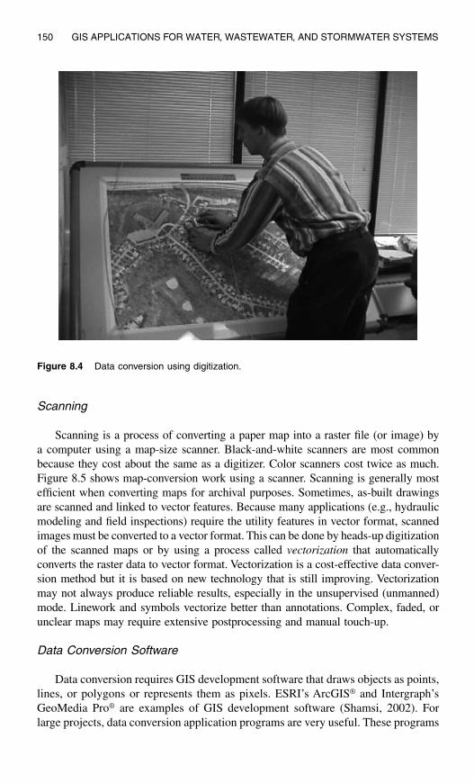
150 GIS APPLICATIONS FOR WATER, WASTEWATER, AND STORMWATER SYSTEMS
Scanning
Scanning is a process of converting a paper map into a raster file (or image) bya computer using a map-size scanner. Black-and-white scanners are most commonbecause they cost about the same as a digitizer. Color scanners cost twice as much.Figure 8.5 shows map-conversion work using a scanner. Scanning is generally mostefficient when converting maps for archival purposes. Sometimes, as-built drawingsare scanned and linked to vector features. Because many applications (e.g., hydraulicmodeling and field inspections) require the utility features in vector format, scannedimages must be converted to a vector format. This can be done by heads-up digitizationof the scanned maps or by using a process called vectorization that automaticallyconverts the raster data to vector format. Vectorization is a cost-effective data conver-sion method but it is based on new technology that is still improving. Vectorizationmay not always produce reliable results, especially in the unsupervised (unmanned)mode. Linework and symbols vectorize better than annotations. Complex, faded, orunclear maps may require extensive postprocessing and manual touch-up.
Data Conversion Software
Data conversion requires GIS development software that draws objects as points,lines, or polygons or represents them as pixels. ESRI’s ArcGIS® and Intergraph’sGeoMedia Pro® are examples of GIS development software (Shamsi, 2002). Forlarge projects, data conversion application programs are very useful. These programs
Figure 8.4 Data conversion using digitization.

MAPPING 151
are usually developed as extensions to standard GIS packages to supplement specificmapping needs. For example, ESRI’s ArcFM water data model supports water andsewer system mapping in a geodatabase. Chester Engineers’ (Pittsburgh, Pennsyl-vania) water editing tool is an application that allows user-friendly mapping of waterand sewer systems for ESRI software users. It eliminates attribute entry and editingvia command prompts or database tables, which require data conversion skills. Userswithout prior data conversion experience can enter attributes from sources documents(e.g., as-built drawings) in a menu environment simply by clicking on points (e.g.,manholes) and lines (e.g., sewers). The water editing tool was developed in several
Figure 8.5 Data conversion using scanning.

152 GIS APPLICATIONS FOR WATER, WASTEWATER, AND STORMWATER SYSTEMS
versions for different users. The ArcView version was developed using Avenue andESRI’s Dialog Designer Extension to support water system and sewer system map-ping needs of the ArcView 3.x users. The ArcInfo 7.x version was written in ArcMacro Language (AML) to support water system and sewer system mapping in anArcedit session. The latest ArcMap version that adds a new water editing toolbar inArcMap was developed using Visual Basic for Applications (VBA) for ArcGIS users.Figure 8.6 shows a screenshot of the ArcMap version of the water editing tool. Theright window shows the form for adding and editing point and line features. Theleft window shows the form for editing point attributes.
Data conversion is started by drawing and attributing the points. After the pointsare attributed, the connecting lines are added from point to point. The applicationprompts the user to select the upstream and the downstream points. After both areselected, the line is added to the data set. By selecting upstream and downstreammanholes to add the lines, the flow direction of a gravity sewer is incorporated intothe data set, ensuring the proper connectivity of the system. Additionally, the linesare snapped to the point features, ensuring that the points of connection correspondto manholes.
Data conversion applications like the water editing tool increase the speed,efficiency, and accuracy of data conversion for water, wastewater, and stormwatersystems. They reduce data-entry errors and can even be used to validate the inputdata. If desired, the applications can be modified to meet the project-specific mappingrequirements.
Figure 8.6 Sample water system data conversion application for ArcMap.

MAPPING 153
Data Processing
Data processing includes some or all of the following tasks:
1. Data preparation2. Topological structuring3. Data management4. Quality control
Data Preparation
This task makes the raw data from source maps or field/GPS surveys availablefor GIS use or GIS-ready. Typical activities include postprocessing of capture data,changing data formats (e.g., from DXF to Shapefile), applying map projections,georeferencing the image data, and/or clipping or mosaicking the aerial photos.
Postprocessing of captured data is warranted if the source maps and the basemap have different accuracy, and captured data do not align with the base map. Inthis case, captured data is edited (moved, stretched, or resized) to fit the base map.
GIS data are stored in various file formats. The number of data formats hasincreased exponentially with the growth in the GIS industry (Goodchild, 2002).According to some estimates, there might be more than 80 proprietary geographicdata formats (Lowe, 2002b). Why are there so many geographic data formats? Onereason is that a single format is not appropriate for all applications. For example, asingle format cannot support both fast rendering in a command and control systemand sophisticated hydraulic analysis in a water distribution system. Different dataformats have evolved in response to diverse user requirements.
GIS software cannot read all the data formats simply because there are so manyformats. Disparate data formats should be converted to one of the formats compatiblewith a particular GIS software. Although many GIS packages provide data conver-sion for the most common data formats, no GIS can support all possible conversions.Many government agencies and data and software companies provide data translatorsfor this purpose (Shamsi, 2002).
Data translation from one format to another can potentially lead to the loss oralteration of data. For instance some platforms can support better numeric precisionthan others. Depending on the mapping scale and the coordinate system, this couldseriously affect data quality. In one system, curves representing a water main mightbe defined mathematically, but in another described as a series of straight linesegments.
Topological Structuring
How much topology should be captured in a GIS map depends on the intendedapplications of the map. For example, in a sewer system modeling application,correct topology (e.g., flow direction) is generally more important than the correctpipe location on the street (e.g., left, right or center of the street). As much topologyas possible should be captured during data conversion. For example, flow direction

154 GIS APPLICATIONS FOR WATER, WASTEWATER, AND STORMWATER SYSTEMS
should be captured if flow direction arrows are shown on source maps. Flow directioncan be automatically captured if sewer pipes are digitized from upstream to down-stream direction. In ArcInfo 7.x “coverage” model, the topology of an arc includesits upstream and downstream nodes (fnode, tnode). ArcInfo 7.x performs computa-tionally intensive topological relationship calculations up front and stores that infor-mation as attributes (fnode, tnode). These attributes are used to determine flowdirection of arcs. If source maps do not have topological relationships or if the dataconversion technicians are not adequately skilled to understand them, topology canbe added after the data conversion by knowledgeable staff. For example, in a waterdistribution system mapping project, valves and hydrants are logically linked to theirappropriate pipe segments by the people who are knowledgeable about systemcharacteristics (Cannistra, 1999).
Conventional GIS packages, such as ArcInfo 7.x and ArcCAD, provide the legacyBUILD and CLEAN commands to build topology and eliminate topological digitizingerrors such as undershoots and overshoots. As shown in Figure 8.7, an undershootoccurs when a line stops short of an intended intersection point and an overshootoccurs when a line extends past an intended intersection point. Traditionally, these“cleaning” operations were done after the data conversion step. Today’s modern GISpackages allow enforcing the topological rules (spatial constraints) during dataconversion and editing. Thus, when a manhole is moved, the topological rules ensurethat the sewers connected to that manhole move simultaneously. For example,ArcInfo 8.3 provides new tools to define, validate, and maintain topology in ageodatabase. Users define which layers participate in a topology and which rulesare appropriate. Topology is stored in a commercial off-the-shelf DBMS.
Data Management
This step organizes attribute data in a database management system (DBMS)format. A GIS database, though not as visible as a GIS map, is an equally critical GIScomponent. The most difficult job in creating a GIS is the enormous effort requiredto enter the large amount of data and to ensure both its accuracy and proper mainte-nance (Walski and Male, 2000). Conventional file-based GIS databases (e.g.,ArcInfo 7.x) store geographic data in vendor-specific proprietary format files. Attribute
Figure 8.7 Common digitizing errors: undershoot (left) and overshoot (right).

MAPPING 155
data are stored in a separate file, which generally has a common nonproprietary format(e.g., a .dbf file). The two separate files are linked using pointers. Modern spatial orobject-oriented databases do not require links between features and attributes becausethey store both the features and attributes in the same file. Incorporating spatial datawith attribute data in a relational database provides a platform for efficient managementof huge data resources, as well as fast and sophisticated spatial query and retrievalmethods (Dalton, 2001).
Quality Control
A comprehensive and well-defined quality assurance/quality control (QA/QC)program should be implemented for large data conversion projects. Data conversionQA/QC can be ensured by checking data completeness, content, symbology, format,structure, and compliance with database specifications during data production. Posi-tional accuracy can be checked using field trips, survey, GPS, photographs, andvideo tapes (Cannistra, 1999).
QA/AC can employ both manual checks and automatic methods. For example,the water editing application shown in Figure 8.6 provides an automatic QA/QCcapability. It displays the points that are completely defined using a white box. Pointsthat have missing attributes are displayed as a box with an X through it. Points thatare added from source drawings are shown as a green box with an X through it.After each point is defined, the list of attributes for each point is displayed on thescreen, allowing the user to double-check the attributes entered for each point.
Data-entry QA/QC can be accomplished by restricting the user input to validdata ranges and rejecting the data entries outside the valid ranges. This capabilitygenerally requires development of custom data-entry forms using computer pro-gramming.
Map Production
The previous steps enable display of GIS layers on the computer screen. Themap production step allows plotting of GIS data on paper and other print media. Itincludes creation of thematic maps using appropriate symbols, colors, patterns, andlegends. For example, water main sizes are shown by different line widths, pressurezones by different colors, and valve types by different symbols. Map productionalso involves printing the scale bar, north arrow, and organization logo. Sometimestables, charts, and photographs are also inserted. Every map should have a title.Other information such as filename, map number, project name and number, plotdate, mapmaker, and map source should also be printed on each important map.
This last step is important because it shows the final result of all the previoussteps. Plotting of GIS maps in the correct style, orientation, scale, size, and formatis a time-consuming process. Plotter speed and network speed are often the mainbottlenecks. Templates for symbology, legends, and layouts should be developed in-house or obtained from other organizations to expedite map production. Somevendors package templates and symbol libraries specific to water, wastewater, andstormwater system with their software products.

156 GIS APPLICATIONS FOR WATER, WASTEWATER, AND STORMWATER SYSTEMS
Maps are needed for map books, wall mounting, archives, presentations, reports,etc. The purpose of the map and the target audience should be considered to designan appropriate map layout. For example, a map for an engineering application shouldbe plotted differently from a map for a water utility newsletter. This step also includesdistribution of the maps to the staff of an organization and optionally to the generalpublic using the Internet, intranet, or wireless technology.
CASE STUDIES
Borough of Ramsey, New Jersey
The Ramsey Board of Public Works is responsible for the operation and maintenanceof water distribution and sanitary sewer collection systems throughout the Borough ofRamsey, New Jersey. In an effort to more efficiently manage its geographically refer-enced data, the board started to explore the benefits and applications of GIS technologyand computer mapping in early 1993. As a first step, with the assistance of ChesterEngineers, Inc. (Pittsburgh, Pennsylvania), the board completed a needs analysis and aGIS pilot project described in Chapter 2 (Shamsi et al., 1995; Shamsi et al., 1996). TheBorough did not have any complete large-scale mapping resources suitable for utilityasset location. System design recommended the following mapping specifications:
• A new digital orthophoto base map should be developed accurate to the tolerancesnormally associated with mapping at a scale of 1 in. = 50 ft.
• Orthophoto base mapping should be established on the New Jersey State PlaneCoordinate System. Survey monuments should be established to enable subse-quent mapping efforts to be tied to the basemap coordinate system.
• Lot and block boundaries should be included as a unique layer in the base map.• Additional map layers for the water distribution system, the sanitary sewer col-
lection system, the stormwater collection system, and census geography shouldbe developed to support other needs of the Borough.
• Use GPS to verify the locations of valves, hydrants, and manholes.
Table 8.2 summarizes the required map layers and the features depicted in eachlayer. Table 8.3 presents the data dictionary for Ramsey’s pilot project.
Table 8.2 Map Layers and Depicted Features
Layer Features
New Jersey State Plane Grid System Grid tics, survey monumentsPhotogrammetric base map Building outlines, street outlines and centerlines,
vegetation, water courses, topographyParcels Lot and block boundariesWater distribution system Mains, valves, hydrantsSanitary sewer collection system Sanitary sewers, manholes, cleanoutsStormwater collection system Storm sewers, manholes, catch basinsCensus geography Blocks, block groups, tracts

MAPPING 157
All of the borough’s sewer system data were stored in a nondigital form. Thisinformation was manually entered into the GIS database. Map features and attributeinformation were gleaned from a variety of sources. Table 8.4 lists recommendedsources for specific map features and attributes. After reviewing the Borough’savailable maps and considering the mapping requirements of the priority applica-tions, the use of digitization was recommended for data conversion.
ESRI’s ArcInfo (Version 6) and ArcView (Version 2) software products were thetwo main software programs used in this project. Because the Borough did not havethe technical staff to maintain an ArcInfo GIS, data conversion work was done bythe consultant using ArcInfo. Due to its low cost, ease of use, and compatibility
Table 8.3 Data Dictionary
Feature Type Required Attributes
Water mains Segment IDPipe materialPipe sizeRepair date(s)Repair type(s)
Water valves Valve IDInstallation dateTypeDate last cycledNormal position
Fire hydrants Hydrant IDAssociated valvesTypeInstallation dateFlow dataPreferred status
Sewers Sewer IDPipe materialPipe sizeFrom manhole IDTo manhole ID
Manholes Manhole IDManhole typeLid typeDepthInflow problem status
Catch basins Catch basin ID
Table 8.4 Source Documents for Map Features and Attributes
Types ofFeatures
Source Documents
Base Map Utility Markouts
Water Systemas Built, 1970,
1:50-Scale
Sewer Systemas Built, 1970,
1:100-Scale
Water mains � �Fire hydrants � � �Water valves � �Sewer pipes � �Manholes � � �Catch basins � � �

158 GIS APPLICATIONS FOR WATER, WASTEWATER, AND STORMWATER SYSTEMS
with the ArcInfo file format, ArcView was installed in the Borough for routinedisplay and plotting of maps and querying the GIS database.
Figure 8.1 shows the Ramsey digital orthophoto base map with an accuracy of± 1.25 ft. The figure on the first page of this chapter shows a map of sanitary sewersand manholes overlayed on the parcel and buildings layers. The sewer features weretaken from as-built drawings and adjusted to locations of surface features that werefield verified. Figure 8.8 shows a water system map with water mains, hydrants, andvalves overlayed on the parcel and buildings layers. Water mains have been classifiedby the diameter attribute of the water main layer.
City of Lake Elsinore, California
Elsinore Valley Municipal Water District located in the city of Lake Elsinore,CA, provides water, wastewater, and agricultural services to approximately 25,000customers. It maintains an infrastructure consisting of 305 mi of water mains, 290 miof sewer pipes, and 246 mi of irrigation pipelines. An ESRI software user since1992, the District migrated to ESRI’s new ArcGIS geodatabase platform in 2000.The migration data conversion work, which included 5000 as-built drawings and300 atlas pages, was completed in 8 months. The source documents were scannedand linked to GIS features. The system has 35 users and employs SQL Server 7relational database management system software, Gateway 7400 and XI NetRAIDerdual 800 MHz servers, and Pentium III workstations. The system maintains approx-imately 75,000 maps in an enterprise GIS environment. GIS allows operations
Figure 8.8 Water distribution system map showing pipes classified by diameter.

MAPPING 159
personnel to create atlas maps and perform asset maintenance, a customer servicedepartment to analyze meter-reading routes and identify illegal connections, and anengineering department to generate as-built construction drawings (ESRI, 2002a).
Allegheny County, Pennsylvania
Each year, sewage overflows affect Pittsburgh’s rivers up to 70 days during theboating season, making water unacceptable for recreational contact. In addition, theoverflows affect Allegheny County’s primary source of drinking water. Municipal-ities in the region could face a potential $2-billion investment in order to correct theproblem. In 2003, the U.S. Environmental Protection Agency (USEPA) issuedadministrative consent orders to 83 municipalities of Allegheny County for control-ling the sewage overflows. The orders required communities to address the sewageoverflow issue through mapping, cleaning, and televising the system, and flowmonitoring. This information will help communities develop a long-term wet-weather control plan. The orders required the following GIS mapping requirements:
• Create an ESRI-compatible base map that includes streets, street names, municipalboundaries, and streams.
• Create an updated ESRI-compatible comprehensive sewer map of the sanitarysewers with the following content:• Location of the sewer lines• Direction of flow• Size of the sewer lines• Sewer line material• Locations of interconnections with other municipal sewer systems• Field-verified location of manholes and catch basins (identified by a compre-
hensive numbering or lettering system)• Location of pump stations, force mains, and siphons• Location of streams or drainage ways tributary to the sewers• Location of overflow (combined sewer overflow [CSO] and sanitary sewer
overflow [SSO]) structures• Locate all significant structures to a minimum horizontal accuracy of 3 ft.• Use as-built drawings, GPS, or traditional land surveying methods to determine
structure locations.• Use State Plane Pennsylvania South NAD83 projection system for coordinates
and NAVD88 datum for elevations.• Manhole inverts and rim elevations to a minimum vertical accuracy of 0.10 ft for
overflow structures, sewers with greater than 10-in. diameters, and other criticalsewers.
• Incorporate field inspection data into comprehensive sewer maps.
USEFUL WEB SITES
Geospatial Information andTechnology Association (GITA)
www.gita.org
USGS GIS Maps for Water Resources water.usgs.gov/maps.htmlUSEPA GIS Information www.epa.gov/epahome/gis.htm

160 GIS APPLICATIONS FOR WATER, WASTEWATER, AND STORMWATER SYSTEMS
CHAPTER SUMMARY
GIS provides powerful capabilities for creating cost-effective and intelligentmaps for water, wastewater, and stormwater systems. The quality of maps dependson data quality, errors, accuracy, scale, and resolution. GIS maps can be developedin many different ways. A mapping approach that best meets the application needsof an organization should be selected. GIS mapping requires five steps: needsanalysis, data collection, data conversion, data processing, and map production.Needs analysis and pilot project testing is highly recommended, as explained inChapter 2 (Needs Analysis). Data conversion is the most time-consuming and costlypart of mapping projects and should be performed carefully. Data conversion appli-cation software can be used to reduce data conversion cost. Digitization and scanningare the two popular methods of data conversion but users can benefit from innovativevariations of these methods. GIS maps should always be constructed in referenceto a base map that has the required accuracy and resolution to support the intendedapplications of GIS maps.
CHAPTER QUESTIONS
1. What are the different types of maps?2. What are the different types of base maps and their characteristics?3. How is a GIS map different from a CAD drawing?4. What is the relationship between map accuracy, scale, and resolution?5. What are the various steps for making GIS maps? Which step is most critical and
why?6. What is data conversion and how is it done?7. What is topology, and how does it affect GIS maps?8. Identify a GIS application in your organization and recommend the appropriate
mapping layers and source documents to implement that application.

161
CHAPTER 9
Mapping Applications
A map is worth a thousand numbers but you must go beyond mappingto sustain your GIS program. This requires putting your GIS maps tobeneficial use.
3D display of sewer system for the Municipality of Bethel Park, Pennsylvania.

162 GIS APPLICATIONS FOR WATER, WASTEWATER, AND STORMWATER SYSTEMS
LEARNING OBJECTIVE
The learning objective of this chapter is to understand the applications of GIS mapsin the water industry.
MAJOR TOPICS
• Common mapping functions• Mapping application examples for water systems• Mapping application examples for wastewater systems• Mapping application examples for stormwater systems
LIST OF CHAPTER ACRONYMS
2-DTwo Two-Dimensional3-DThree Three-DimensionalCOGO Coordinate GeometryCSO Combined Sewer OverflowDEM Digital Elevation ModelDTM Digital Terrain ModelI/I Inflow/InfiltrationMS4 Municipal Separate Storm Sewer SystemNPDES National Pollution Discharge Elimination SystemSQL Structured Query LanguageTIN Triangular Irregular Network/Triangulated Irregular Network
This book focuses on the four main applications of GIS, which are mapping, monitor-ing, modeling, and maintenance and are referred to as the “4M applications.” In this chapterwe will learn the applications of the first M (mapping).
CUSTOMER SERVICE APPLICATION IN GURNEE
The Village of Gurnee, located near Chicago (Illinois), has seen explosive growthsince the 1970s. Population more than doubled from 13,701 in 1990 to 28,834 in2000. This growth bogged down Gurnee personnel with public meetings, rezoninghearings, code violations, road construction, and water line and sewer line repairs.Several departments were legally required to notify property owners of meetings,pending changes, or future disruptions. The Village used GeoMedia GIS softwarefrom Intergraph to automate the resident notification process (Venden and Horbinski,2003). The automated system — known as Notifast™ — allows staff members toenter a street address or select a parcel, specify a distance radius, and identify allproperty owners within that distance. Notifast then generates a list of mailing labels

MAPPING APPLICATIONS 163
and mail-merged form letters. Each letter includes an embedded map that clearlyshows the area in question. This application of existing GIS maps has improvedefficiency and customer service. What used to take hours is now completed inminutes.
Figure 9.1 shows a screenshot of how parcels can be selected in ESRI’s ArcGISsoftware by drawing a circle. The 200-ft radius circle is drawn with its center at theproject site. All the parcels that are intersected by the circle are selected as shownin the hatched pattern. The attribute data for the selected parcels are shown in thetable to the left of the circle. These data can be copied in a word processor’s mail-merge feature to generate notification letters.
As explained in Chapter 8 (Mapping), creation of GIS maps is a huge undertak-ing. Unfortunately, in today’s competitive world, despite the enormous effortrequired to create them, colorful maps alone can no longer justify the existence ofa GIS program. This is because, after spending large sums of money on a mappingproject, many water and sewerage agencies are wondering what else to do with theirGIS maps. To garner continued financial support for a GIS program, GIS programsmust go beyond conventional map printing activities and demonstrate the usefulness(applications) of GIS maps. This chapter shows how to do that.
It does not occur to most people that a good map raises more questions than it answers —that the question of why things are located where they are raises important intellectualissues, with immediate serious implications. (Lewis, 1985).
Figure 9.1 Selecting notification parcels in ArcGIS.

164 GIS APPLICATIONS FOR WATER, WASTEWATER, AND STORMWATER SYSTEMS
A paper map provides the power of place but a map in GIS can automate “thewhy of where.” Most GIS applications originate from GIS maps. This chapterdescribes simple mapping applications. Advanced applications like hydrologic andhydraulic modeling, facilities management, inspection and maintenance, and plan-ning are described in other chapters.
COMMON MAPPING FUNCTIONS
Most GIS packages provide simple data analysis capabilities that can be usedto create basic mapping applications without custom programming. Typical examplesof these GIS functions are given in the following subsections.
Thematic Mapping
Thematic mapping is one of the easiest ways to develop mapping applications.Map components can be logically organized into sets of layers called themes. A themeis a group of similar geographic features, such as hydrants (points), water mains(lines), or pressure zones (polygons). These themes can be manipulated using clas-sification and legend (symbology) to create different thematic maps. Classificationplaces attribute values into groups. For example, water mains for a city can beclassified by diameter to create groups such as pipes smaller than 6 in., pipes 8 to12 in., and pipes greater than 12 in. These groups can then be displayed using differentlegends reflecting different colors, line thicknesses, and symbols (e.g., solid, dashed,or dotted lines). Each combination of a classification method and legend will producea different thematic map. Figure 9.2 shows the difference between an unclassifiedand nonsymbolized sewer map (top) and the same map classified and symbolized bypipe diameters (bottom). Obviously, the bottom map will be more useful in applica-tions that require pipe diameters, such as flow monitoring and hydraulic modeling.
Spatial Analysis
Many GIS packages also allow users to select the features of one or more themesusing the features of another theme. Referred to as spatial or overlay analyses, thesetheme-on-theme selection functions identify whether one feature lies within another,whether it completely contains another, or whether it is within a specified distanceof another, and so on. For example, these mapping operations can identify themanholes in a given drainage basin, or census blocks within a watershed, or theproperties within a certain distance of a water main.
Buffers
A buffer can be created around one or many features by using the buffer functiontypically found in most GIS packages. Creating a buffer provides a visual represen-tation on a map of the area within a certain distance of one or more features. Buffercan also be used to select features in other layers that fall within the buffered area.

MAPPING APPLICATIONS 165
Figure 9.2 A sewer system map. Above: without attribute classification and symbology; below:with attribute classification and symbology for pipe diameter.
Sewersp.shp<all other values>
DIAM24"20"18"16"15"12"10"6"8"4"

166 GIS APPLICATIONS FOR WATER, WASTEWATER, AND STORMWATER SYSTEMS
For instance, a buffer can be drawn to show the area around a well that is contam-inated or to represent a floodplain around a river. Figure 9.3 shows a buffer createdaround existing combined sewers in the Borough of Kittanning, Pennsylvania. Itidentifies the area targeted for sewer separation in the Borough’s combined seweroverflow (CSO) control plan.
Figure 9.3 Buffer for a sewer separation project.

MAPPING APPLICATIONS 167
Hyperlinks
Some GIS packages such as ArcView and ArcGIS have Hotlink or Hyperlinkfunctions respectively to provide additional information about the features. Forexample, when a feature is clicked with the Hyperlink tool, a document or file islaunched using the application associated with that file type. This function can beused as a document management system from within a GIS. For example, userscan click on a valve to display the valve card, on a sewer pipe to launch a televisedvideo file, or on a water main to display its as-built drawing. Figure 9.4 shows adisplay of a scanned image of a water distribution system valve parts list usingArcView’s Hotlink function. Additional information on hyperlinks is provided inChapter 15 (Maintenance Applications).
WATER SYSTEM MAPPING APPLICATIONS
Representative mapping applications for water distribution systems are given inthe following subsections.
MWRA Water System Mapping Project
In the late 1990s the Massachusetts Water Resources Authority (MWRA) con-ducted a major in-house effort to develop a linked system schematic set. Theseoverview maps did not have a scale or base, but showed how the elements of thesystem connected hydraulically. In addition to developing the digital version of thesemaps, the GIS staff created links to a number of real time databases and the locationplans for each valve. Thus, the schematic showed the status of all mainline valvesfor emergency response planning. If a valve was inoperable or had been opened orclosed, the GIS updated the color of the pipe line on the schematic, alerting theusers to its condition.
MWRA then consolidated their water distribution facility data and source docu-ment references into a manageable set of data tables and digital maps that were easilyaccessible to MWRA staff. They also linked the records of every pipe, valve, meter,and fitting in the distribution system to existing databases of record plans, land takings,hydraulic conditions, leaks, maintenance activities, and schematic representations inthe GIS. This effort allowed MWRA users to click on a pipe drawing, and instead ofbeing able to access just the record drawing, choose from a menu of options regardingthe land records and model scenarios, as well as the physical condition and mainte-nance history of the pipe. This provided access to a variety of maintenance and datadevelopment activities throughout the water division (Estes-Smargiassi, 1998).
Service Shutoff Application
To strengthen enforcement activities on delinquent accounts, the PhiladelphiaWater Department (PWD) developed an ArcView GIS tool to support its shutoffprogram. The shutoff tool identifies priority sites and automates crew assignments

168 GIS APPLICATIONS FOR WATER, WASTEWATER, AND STORMWATER SYSTEMS
to increase crew productivity. A prioritizing algorithm identifies delinquent cus-tomers based on age and amount in arrears. These priority accounts identifyclusters of shutoff sites. Clusters are formed using ArcView Network Analystextension to locate nearby sites reachable by the street network. The applicationgenerates maps and tables for each crew’s daily schedule. With the help of this
Figure 9.4 Hotlink function displaying valve information for a water distribution system.

MAPPING APPLICATIONS 169
application and other measures, PWD improved enforcement efficiency by 60%(Lior et al., 1998).
Generating Meter-Reading Routes
Seattle Public Utilities (SPU) has more than 174,000 customers. In an effort tosave meter-reading cost and improve customer service, GIS was used to create moreefficient meter-reading routes. In 1995, SPU’s Metering and GIS departments joinedforces to explore the feasibility of rerouting meter-reading routes. In 1997, a pilotproject was completed using software from ESRI and RouteSmart Technologies,which convinced the SPU management to implement a citywide rerouting project.The project implementation resulted in cost savings for the ratepayer, especiallybecause of SPU’s prior investments in GIS data conversion (Lee, 1998).
Map Maintenance Application
In Ohio, Cincinnati Water Works (CWW) developed a GIS application for waterdistribution system maintenance, hydraulic modeling, and customer service. A majorcomponent of this application was the development of a Map Maintenance Application(MMA), which is an update developed using ArcInfo and Oracle. It allows simulta-neous maintenance of water system layers and related RDBMS tables. The MMAfeatures COGO data entry, scroll lists for table inserts, and feature abandonment. Italso utilizes the integrity constraint checking capability of the RDBMS (Guetti, 1998).
WASTEWATER SYSTEM MAPPING APPLICATIONS
Representative mapping applications for wastewater systems are given in thefollowing subsections.
Public Participation with 3D GIS
At the present time many cities in the U.S. are planning to spend billions ofdollars to meet the regulatory requirements for correcting their wastewater problems,such as wet-weather overflows from the sewer systems. Given the potential forsignificant expenditures of public funds, a key to the future success of capital projectsis public participation. The regulatory agencies are mandating public participationas a required element of these projects. Therefore, establishing early communicationwith both the public and the regulatory agencies should be an important first stepin a long-term planning approach, and crucial to the success of a wastewater capitalimprovement program. By informing the public early on in the planning processabout the scope and goals of the program, and continuing this public involvementduring development, evaluation, and selection of alternatives, issues and potentialconflicts can be identified and addressed more expeditiously, minimizing the poten-tial for prolonged delay or additional cost.
Three-dimensional (3D) maps are an effective means of public education, noti-fication, and communication. They provide impressive “real-life” visions of proposed

170 GIS APPLICATIONS FOR WATER, WASTEWATER, AND STORMWATER SYSTEMS
projects. GIS, CAD, and multimedia technologies can be combined to produce 3Dmodels and 3D animations.
3D maps can be created by adding elevation data to existing 2D vector layers.Elevation data can be obtained from contour maps, digital elevation models (DEM),digital terrain models (DTM), aerial surveys, engineering drawings, or GPS surveys.The quality of 3D analysis largely depends on the accuracy and resolution ofelevation data. For engineering design, highly accurate data are required. For pre-sentation mapping, less accurate data can be used. For example, in-lieu of accurateheights, buildings can be elevated in proportion to the number of floors.
GIS fly-through scenes allow the public to experience a 3D walk-through of aproposed project. Animation can animate objects within a model, e.g., cars movingdown the road or people walking on the curbs. Realistic materials and textures canbe added to depict the actual field conditions, e.g., wet streets. Climatic conditions,e.g., snow cover or sunlight can be added to portray the specific design conditions.
3D capability is usually added to standard GIS packages by installing additional3D extensions or modules. For example, 3D Analyst Extension enables ESRI’sArcGIS users to visualize and analyze surface data. Using 3D Analyst, one can viewa surface from multiple viewpoints, query a surface, determine what is visible froma selected location on a surface, and create a realistic perspective image drapingraster and vector data over a surface.
The figure on the first page of this chapter shows a 3D map of a sewer systemfor the Municipality of Bethel Park, Pennsylvania. Created using 3D Analyst Exten-sion, the map shows buildings, contours, and sewer lines overlaid on an aerialphotograph. Because wastewater must flow down the hill, design of gravity sewersdepends on topography. GIS can help create 3D maps to facilitate efficient engi-neering of a new sewer system, quick assessment of an existing sewer system, orpresentation of the project layout to the general public.
Figure 9.5 shows a 3D fly-through animation of an Allegheny County SanitaryAuthority (ALCOSAN) sewer construction project in the City of Pittsburgh, Penn-sylvania. Completed in 1999, this $24-million project involved construction of a5.2-mi-long parallel relief interceptor to relieve sewer overflows and basement flood-ing in the Saw Mill Run Watershed of the city. The pipe sizes for the relief interceptorranged from 36 to 54 in. in diameter. The parallel interceptor was designed to followthe alignment of the Saw Mill Run Creek because the right-of-way corridor alongthe main street (Route 51) was not conducive to a major interceptor constructionproject. Animation was used to present the project design in a general public meeting.Figure 9.5 shows the sewers and manholes exposed above the ground surface tohelp the general public envision the proposed interceptor layout. The animationclearly indicated that the new sewers will mostly avoid backyards, parking lots, androads — an issue that was very important to the residents of the community. Thisapproach helped ALCOSAN to win the public support for the project.
Mapping the Service Laterals
Recent inflow and infiltration (I/I) studies have shown that service laterals areone of the most significant I/I contributors, generating as much as 60% of the total

MAPPING APPLICATIONS 171
I/I quantity. Unfortunately, most collection systems do not have maps of their servicelaterals. TV inspection logs provide accurate lateral location information, which canbe used to prepare service lateral GIS maps. For example, Chester Engineers (Pitts-burgh, Pennsylvania) developed a Wyemaker ArcView extension to add service wyes(Ys) to sewer lines. Developed using ArcView Dialog Designer extension, this utilityis a good example of GIS customization.
Figure 9.6 shows a typical two-page TV inspection log. The first page providesgeneral information about a sewer pipe. The second page details the specific pipedefects and their location. This page also includes the location of service lateralsmeasured in feet from one manhole to the next. The Wyemaker extension will firstcreate a database containing the wye information for each sewer main. The wyeinformation is entered in a wye input form shown in Figure 9.7 that basicallyreplicates the data fields on the log sheets. The upstream and downstream manholeidentification numbers are entered. In this case, the sewer segment ID is created byconcatenating the upstream and downstream manholes. The sewer length from theinspection log is entered as well as the beginning distance (usually zero). The userthen indicates the direction of the measurements, the wye measurement and the sideof the line in which the wye is located. The direction of the measurements is thedirection in which the line was inspected. The direction is either “against the flow”(from the downstream manhole to the upstream manhole) or “with the flow” (from
Figure 9.5 3D fly-through animation of a sewer construction project.

172 GIS APPLICATIONS FOR WATER, WASTEWATER, AND STORMWATER SYSTEMS
Figure 9.6 Sample TV inspection log.
Figure 9.7 Service laterals view in ArcView.

MAPPING APPLICATIONS 173
the upstream manhole to the downstream manhole). Entering the direction ofmeasurement and the side of the line eliminates the need for the user to recalculatedistances if the line was measured against the flow. The calculations are automaticallydone by the extension and the position of the wye (right or left) is automaticallyswitched if necessary. Once the form is completed, the user simply clicks on “SaveRecord” and the wye record is automatically saved to the wye table.
When all records are entered, the database table is used to create a Shapefile ofthe wyes. All the wyes in the Shapefile are exactly the same length and at the exactsame angle from the sewer line, creating an aesthetically appealing data set. Thewyes are kept in a separate Shapefile rather than being added to the existing sewertheme in order to maintain the connectivity of the main lines. A sample lateral mapcreated using this method is shown in Figure 9.7.
Additional examples of wastewater system mapping applications are includedin Chapter 15 (Maintenance Applications).
STORMWATER SYSTEM MAPPING APPLICATIONS
A representative mapping application for stormwater systems is presented below.
Stormwater Permits
In the U.S., many cities with storm sewers and outfalls must comply with aNational Pollution Discharge Elimination System (NPDES) Stormwater Permitunder the U.S. Environmental Protection Agency’s Municipal Separate Storm SewerSystem (MS4) permit program. These permits require U.S. municipalities to developstormwater pollution prevention programs, track the compliance schedules, andmonitor stormwater system maintenance and water quality sampling.
Some cities finance the operation of a stormwater utility that pays for permitcompliance by assessing a stormwater fee (drainage tax) on the properties. Initially,some U.S. municipalities chose to implement a flat tax for all property owners, basedon the tax value of their property. Because only the impervious area of a propertycontributes to stormwater runoff, many cities used a more equitable approach thatassessed the tax in proportion to the impervious area of each property. Accuratecalculation and tracking of impervious areas from conventional methods (e.g., fromsurvey or paper maps) is cumbersome and costly. GIS allows accurate and inexpen-sive capture of impervious surfaces from aerial photographs, orthophotos, scannedsite plans, and parcel maps.
GIS can be used to develop stormwater user fees using the following steps:
1. Delineate property land covers using digital orthophotos.2. Assign a percent imperviousness factor to each land cover. For example:
• Roofs, 100%• Concrete driveway, 100%• Gravel driveway, 75%• Parking lot, 90%

174 GIS APPLICATIONS FOR WATER, WASTEWATER, AND STORMWATER SYSTEMS
3. Estimate land-cover area-weighted mean percent imperviousness of each property.4. Determine stormwater rates based on mean percent imperviousness of a property
rather than the total impervious area.
For example, the Texas legislature passed a law allowing municipalities to createdrainage utilities that assessed utility fees associated with each land parcel based onthe amount of stormwater runoff it contributed. The City of Irving, Texas, startedusing GIS and color-infrared aerial photography in 1993 to examine and map thesources of the city’s stormwater runoff. The City assumed that a simple distinctionbetween pervious surfaces such as vegetative cover and impervious surfaces suchas buildings and parking lots would be sufficient to determine the stormwater runoffof each parcel with acceptable accuracy. To determine the area of each surface typewith individual parcels, the tax-parcel layer was overlaid with the pervious/imper-vious layer. This operation created a list of each parcel’s tax identification numberand the associated pervious/impervious area. This table was then linked to the City’swater utility billing system to calculate the amount due from each property ownerand include that amount in the monthly utility bill (American City&County, 1994).
The City and County of Denver, Colorado, has a storm drainage utility thatassesses a fee on all properties in Denver based on the amount of impervious surfacepresent on each property, as well as on the percentage of the total area of each propertythat the impervious surface represents. Initially, Denver used field measurements butdid not find them cost-effective. In 2002, they hired the Denver firm of Elroi Con-sulting, Inc., to implement an impervious surface GIS for the County. Initially, thesystem was implemented using ArcGIS 8.1 and a personal geodatabase that requiredonly ArcView licenses. The system was later upgraded to work with an ArcSDEgeodatabase, complete with versioning and multiuser editing. The system builds onthe ArcMap component of ArcGIS, both removing unnecessary toolbars from theuser interface and adding several custom toolbars. The user-friendly interface enableseven the non-GIS users (e.g., field inspectors) to use the system. Impervious surfacesare digitized directly into the GIS, thus making impervious surface fee assessmentsdefensible. The impervious surface GIS was subsequently linked to Denver’s storm-water billing system for rapid database update. With this system, Denver now collectsover $12 million annually in impervious surface fees (Elroi, 2002).
Oakland County, Michigan, which has more than 440,000 parcels, uses high-density spot elevation and break-line data in GIS to create triangular irregularnetwork (TIN) surface models. These models help the county drain commissioner’soffice to visualize the terrain and delineate catchment areas. This approach identifiesprecise drainage patterns and the land that contributes runoff to a storm drain. Thecatchments define the drainage district boundaries that are used to assess the appro-priate drainage tax in an equitable manner (Gay, 2003).
The conventional paper-based permit compliance approach can be very hecticfor large cities. GIS is being used in many U.S. cities to meet the stormwater permitrequirements system in a user-friendly environment. For example, SQL, Avenue,and Dialog Designer have been utilized to develop an interface between ArcViewGIS and Microsoft Access for developing an NPDES compliance application (Huey,1998). This application is helping both the management of stormwater features such

MAPPING APPLICATIONS 175
as sewer lines and outfalls, and preparation of complex NPDES Annual Reports.The report requires summarizing all stormwater management program goals andefforts toward meeting those goals. An example of the use of dialogs and custom-programmed icon buttons for query is shown in Figure 9.8.
CHAPTER SUMMARY
Paper maps are useful but their applications are limited. In most cases, mapmak-ing alone cannot justify the continued financial support for a GIS department. GISmaps and associated databases can be manipulated in a variety of ways to developapplications that automate and simplify the routine tasks. GIS maps are the startingpoint for developing GIS applications: no maps, no applications. In this chapter welearned about some basic applications of GIS maps. Advanced applications will bepresented in subsequent chapters.
CHAPTER QUESTIONS
1. What is the meaning of “beyond mapping?” Why is it important to go beyondmapping?
2. Compile a list of ten mapping applications.3. Using literature review or the Internet, write a 200-word example of a mapping
application for a water distribution system not described in this chapter.4. Repeat Question 3 for a wastewater collection system.5. Repeat Question 3 for a storm drain system.
Figure 9.8 Utilization of dialogs to monitor and update structure-maintenance activities.


177
CHAPTER 10
Monitoring Applications
GIS is ideally suited to install, maintain, and query monitoringequipment such as, rain gauges, flow meters, and water qualitysamplers for system physical and hydraulic characterization. GISallows display and analysis of monitoring data simply by clicking ona map of monitoring sites.
Gauging and inspection stations in the city of Los Angeles, California.

178 GIS APPLICATIONS FOR WATER, WASTEWATER, AND STORMWATER SYSTEMS
LEARNING OBJECTIVE
The learning objective of this chapter is to familiarize ourselves with GIS applicationsin monitoring data for effective operation and management of water, wastewater,and stormwater systems.
MAJOR TOPICS
• Rainfall monitoring• Satellite and radar rainfall data• Flow-monitoring applications• Permit reporting applications• Internet monitoring applications• Infrastructure monitoring applications
LIST OF CHAPTER ACRONYMS
CCTV Closed Circuit TelevisionGML Geography Markup LanguageHRAP Hydrologic Rainfall Analysis Project (a map projection system)NCDC National Climatic Data Center (U.S.)NEXRAD Next Generation Weather RadarNOAA National Oceanic and Atmospheric Administration (U.S.)NPDES National Pollution Discharge Elimination System (U.S.)NWS National Weather ServiceOGC Open GIS ConsortiumSCADA Supervisory Control and Data Acquisition SystemsWSR Weather Surveillance Radar
This book focuses on the four main applications of GIS, which are mapping, monitor-ing, modeling, and maintenance and are referred to as the “4M applications.” In this chapterwe will learn about the applications of the second M (monitoring).
MONITORING REAL TIME RAINFALL AND STREAM-FLOWDATA IN AURORA
The city of Aurora, Colorado, is a community of approximately 247,000 peoplelocated in the southeast Denver metro area. The City’s Utilities Department usedESRI’s ArcInfo and ArcView software to analyze and display real time rain-gauge andstream-flow data from the City’s ALERT Flood Warning System. Data were obtainedby querying a remote real time data-collection database. The Utilities Department wasable to access and analyze both historical and current real time rainfall and stream-flow data from an easy-to-use graphical interface. ArcView’s Spatial Analyst Extensionwas used to develop a continuous areal rainfall surface from the point rainfall data.This allowed a better and clearer understanding of a particular storm and allowed a

MONITORING APPLICATIONS 179
more complex analysis of the true impact of the storm event. Applications of thisprogram included studies in emergency flood response, location of flood reports,routine maintenance for storm sewers, and National Pollution Discharge EliminationSystem (NPDES) compliance for water quality (Rindahl, 1996).
MONITORING BASICS
Monitoring of various types of data is essential to the effective management ofwater, wastewater, and stormwater systems. Generally, two types of data are required:(1) physical characterization data and (2) hydraulic characterization data. Physicalcharacterization data describe the physical condition of the infrastructure, such aspipe and manhole conditions. Examples of physical characterization data sourcesinclude closed-circuit television (CCTV) inspection of pipes, manhole inspections,and smoke-testing of buildings. GIS applications for these types of data are describedin Chapter 15 (Maintenance Applications).
Hydraulic characterization data describe the quantity and quality of flow throughpipes and open channels as well as meteorological factors impacting the flow, such asprecipitation.
Wastewater and stormwater systems typically require data on flow quantity(depth, velocity, flow rate, and volume), quality (e.g., suspended solids and bacteria),and rainfall. Figure 10.1 shows a flowmeter and weir installation in a combinedsewer system overflow manhole. The flowmeter (Flo-Dar from Marsh-McBirney,Inc.) shown on the left records incoming combined sewage depth, velocity, and flowdata. The weir shown on the right collects outgoing overflows. Some wastewaterand stormwater hydrologic and hydraulic (H&H) models require data on addi-tional meteorological parameters such as ambient temperature, evaporation rate,and wind speed. Water distribution systems typically require water pressure andwater quality data. In many projects, monitoring tasks make up a significant portionof the scope of work and could cost 20 to 30% of the total budget. Careful installationof monitors and effective management of monitoring data is, therefore, highlydesirable for the on-time and on-budget completion of monitoring projects.
GIS is ideally suited for selecting the best sites for installing various hydrauliccharacterization monitors. Once the monitors have been installed, GIS can be usedto query the monitored data simply by clicking on a map of monitoring sites. GIScan also be used to study the spatial trends in the monitored data. GIS is especiallyuseful in processing and integrating radar rainfall data with H&H models of sewagecollection systems and watersheds. This chapter will present the methods and exam-ples of how to use GIS for installing and maintaining the monitors, and for queryingand analyzing the monitoring data.
REMOTELY SENSED RAINFALL DATA
Many watersheds, especially those smaller than 1000 km2, do not have recordingrain gauges capable of recording at hourly or subhourly intervals. Sometimes raingauges exist, but data are found missing due to equipment malfunction. Quite often,

180 GIS APPLICATIONS FOR WATER, WASTEWATER, AND STORMWATER SYSTEMS
rain-gauge density is not adequate to accurately capture the spatial distribution ofstorm events. Such data gaps can be filled by the rainfall data provided by weathersatellites and radars, as described in the following subsections.
Satellite Rainfall Data
Direct measurement of rainfall from satellites is not feasible because satellitescannot penetrate the cloud cover. However, improved analysis of rainfall can beachieved by combining satellite and conventional rain-gauge data. Meteorologicalsatellites such as the NOAA-N series, those of the Defense Meteorological SatelliteProgram, and U.S. geostationary satellites can observe the characteristics of cloudswith precipitation-producing potential and the rates of changes in cloud area andshape. Rainfall data can now be estimated by relating these cloud characteristics toinstantaneous rainfall rates and cumulative rainfall over time. Cloud area and tem-perature can be used to develop a temperature-weighted cloud cover index. Thisindex can be transformed to estimate mean monthly runoff values. Satellite rainfallestimating methods are especially valuable when few or no rain gauges are available(ASCE, 1999).
Figure 10.1 Flowmeter and weir installation in a manhole for monitoring incoming and out-going flows.

MONITORING APPLICATIONS 181
Radar Rainfall Data
Weather radars provide quantitative estimates of precipitation, which can be usedas input to H&H models. Radar rainfall estimates augmented with data from sparserain-gauge networks are useful in H&H modeling. Weather radars provide real time,spatially distributed rainfall data that can be extremely valuable for flood forecastingand flood warning.
NEXRAD Rainfall Data
The U.S. National Weather Service (NWS) has a group of weather radars calledthe Next Generation Weather Radar (NEXRAD) system. NEXRAD comprisesapproximately 160 Weather Surveillance Radar–1988 Doppler (WSR-88D) sitesthroughout the U.S. and selected overseas locations. This system is a joint effort ofthe U.S. Departments of Commerce (DOC), Defense (DOD), and Transportation(DOT). The controlling agencies are the NWS, Air Weather Service (AWS), andFederal Aviation Administration (FAA), respectively. Level II data provide threemeteorological base data quantities: reflectivity, mean radial velocity, and spectrumwidth. These quantities are processed to generate numerous meteorological analysisproducts known as Level III data. Level II data are recorded at all NWS and mostAWS and FAA WSR-88D sites. Level III products are recorded at the 120 NWSsites. The data are sent to the National Climatic Data Center (NCDC) for archivingand dissemination.
NEXRAD Level III Data
There are a total of 24 Level III products routinely available from NCDC,including 7 graphic products in clear-air mode, 11 in precipitation mode, 5 graphicoverlays, and 1 alphanumeric product. Each product includes state, county, and citybackground maps. Level III graphic products are available as color hard copy,grayscale hard copy, or acetate overlay copies. A brief description and possible usesof these products are given below:
• Base Reflectivity (R): A display of echo intensity measured in dBZ (decibels ofZ, where Z represents the energy reflected back to the radar). This product is usedto detect precipitation, evaluate storm structure, locate boundaries, and determinehail potential.
• Base Spectrum Width (SW): A measure of velocity dispersion within the radarsample volume. The primary use of this product is to estimate the turbulenceassociated with mesocyclones and boundaries.
• Base Velocity (V): A measure of the radial component of the wind either towardthe radar (negative values) or away from the radar (positive values). Negativevalues are represented by cool colors (green), whereas positive values are repre-sented by warm colors (red). This product is used to estimate wind speed anddirection, locate boundaries, locate severe weather signatures, and identify sus-pected areas of turbulence.

182 GIS APPLICATIONS FOR WATER, WASTEWATER, AND STORMWATER SYSTEMS
• Composite Reflectivity (CR): A display of maximum reflectivity for the totalvolume within the range of the radar. This product is used to reveal the highestreflectivities in all echoes, examine storm structure features, and determine theintensity of storms.
• Echo Tops (ET): An image of the echo top heights color-coded in user-definedincrements. This product is used for a quick estimation of the most intenseconvection and higher echo tops, as an aid in identification of storm structurefeatures, and for pilot briefing purposes.
• Hail Index Overlay (HI): A product designed to locate storms that have thepotential to produce hail. Hail potential is labeled as either probable (hollow greentriangle) or positive (filled green triangle). Probable means the storm is probablyproducing hail and positive means the storm is producing hail.
• Mesocyclone Overlay (M): This product is designed to display information regard-ing the existence and nature of rotations associated with thunderstorms. Numericaloutput includes azimuth, range, and height of the mesocyclone.
• One-Hour Precipitation (OHP): A map of estimated 1-h precipitation accumu-lation on a 1.1 nmi
× 1.1 nmi grid. This product is used to assess rainfallintensities for flash flood warnings, urban flood statements, and special weatherstatements.
• Severe Weather Probability Overlay (SWP): A measure of a storm’s relativeseverity as compared with those around it. The values are directly related to thehorizontal extent of vertically integrated liquid (VIL) values greater than aspecified threshold. This product is used for quick identification of the strongeststorms.
• Storm Structure (SS) (alphanumeric product): A table displaying information onstorm attributes that include maximum reflectivity, maximum velocity at lowestelevation angle, storm overhang, mass-weighted storm volume, storm area baseand top, storm position, and storm tilt.
• Storm Total Precipitation (STP): A map of estimated storm total-precipitationaccumulation continuously updated since the last 1-h break over the entire scope.This product is used to locate flood potential over urban or rural areas, estimatetotal basin runoff, and provide rainfall data 24 h a day.
• Storm Tracking Information Overlay (STI): A product that shows a plot of thepast hour’s movement, current location, and forecast movement for the next houror less for each identified thunderstorm cell. This product is used to determinereliable storm movement.
• Tornadic Vortex Signature Overlay (TVS): A product that shows an intense gate-to-gate azimuthal shear associated with tornadic-scale rotation. It is depicted bya red triangle with numerical output of location and height.
• VAD Wind Profile (VWP): A graphic display of wind barbs plotted on a heightstaff in 500-ft or 1000-ft increments. The current (far right) and up to ten previousplots may be displayed simultaneously. This product is an excellent tool formeteorologists in weather forecasting, severe weather, and aviation.
• Vertically Integrated Liquid (VIL): The water content of a 2.2 nmi
× 2.2 nmicolumn of air, which is color-coded and plotted on a 124 nmi map. This productis used as an effective hail indicator to locate most significant storms and toidentify areas of heavy rainfall.
NEXRAD data and various visualization and analysis software tools areavailable from NCDC and commercial vendors.

MONITORING APPLICATIONS 183
Estimating Rainfall Using GIS
Because rainfall is a critical component in conducting H&H analyses, thequality of rainfall data is critical for accurate system hydraulic characterization.It is often the case that the spatial distribution of rain-gauges over a collectionsystem is too sparse to accurately estimate the rainfall over a given basin. Radarrainfall technology can be used to obtain high-resolution rainfall data over anapproximately 2 km
× 2 km area (called a pixel). GIS can be used to display andprocess the radar rainfall data.
NEXRAD Level III data from Doppler radar measurements provide spatiallydense rainfall data. These data are similar to those commonly seen on weather maps.Such data do not require interpolation between point data from widely scattered rain-gauges because they provide continuous rainfall measurements throughout a watershedor sewershed (Slawecki et al., 2001).
WRS-88D radar images have a mean resolution of 4 km
× 4 km. They areregistered to the Hydrologic Rainfall Analysis Project (HRAP) map projection sys-tem. The radar rainfall data can be incorporated in a GIS-based distributed hydrologicmodel by importing it in a raster grid format. However, this may require reprojectingthe rainfall grid from the HRAP coordinate system to the coordinate system beingused by the model.
The accuracy of radar rainfall estimates can be improved substantially by cali-brating the radars using the point rain-gauge observations. Generating NEXRADrainfall estimates requires extensive expertise and computational resources (ASCE,1999). Hourly NEXRAD rainfall data called hourly digital precipitation array (DPA)are available from several NWS-authorized commercial data vendors, such as WSICorporation and Paramax Systems Corporation. Weather data vendors such as DTNWeather Services (now part of Meteorlogix, Inc.) provide continuously updated, realtime, GIS-ready, georeferenced weather data in ESRI GRID (raster) and Shapefile(vector) formats and georegistered TIFF format to weather-enable the GIS applicationsfor water and wastewater utilities. The DTN data include 5-min NEXRAD updates andstorm cell type, severity, speed, and direction. Meteorlogix provides weather extensionsfor ESRI’s ArcGIS software package. NEXRAIN Corporation (Orangevale, Califor-nia) provides georeferenced polygon Shapefiles of radar pixels over a given studyarea. Each radar pixel is given a unique ID field, which can be used to visualize andanalyze rainfall data from a separate text or database file. Shapefiles are projectedinto the user-specified coordinate system. NEXRAIN-2k product is extracted froma national mosaicked data set of 2-km radar data, updated every 15 min. Figure 10.2shows a Shapefile of the NEXRAIN-2k radar pixels in Colorado State Plane Central(NAD83 ft) over Colorado Springs, Colorado, for a storm event on August 31, 2001.The top-left window shows rainfall distribution at 2 A.M.; the top-right windowshows rainfall distribution at 5 P.M.; the bottom-left window shows rainfall distri-bution at 8 P.M.; the bottom-right window shows the attribute table; the top-centerwindow shows the results of a pixel query; and the bottom-center insert shows arainfall map overlaid on a street map.
WSI Corporation, a supplier of weather data in the U.S., provides the WSIPRECIP data over these pixels in 15-min time increments. These data can be obtained

184 GIS APPLICATIONS FOR WATER, WASTEWATER, AND STORMWATER SYSTEMS
through commercial vendors and adjusted to reliable ground gauges, if necessary.Hence, the radar rainfall volume adjusted through calibration with ground gauge,combined with high-resolution spatial distribution, provides modelers with a veryaccurate local estimate of rainfall. These estimates can be used with their flowme-tering to characterize the basin of interest (Hamid and Nelson, 2001).
Radar Rainfall Application: Virtual Rain-Gauge Case Study
Precipitation varies with time and across a watershed. GIS can easily create arainfall contour map from point rainfall values. Unfortunately, point rainfall valuesare generally scarce due to inadequate rain-gauge density. Many watersheds havefew or no rain gauges to accurately measure the spatial rainfall distribution. In thiscase, a hydrologist may have to use the precipitation data from a nearby watershed.Many watersheds do not have recording-type rain gauges to measure the hourlyvariation of precipitation. In this case, a hydrologist may need to apply the temporaldistribution of a nearby watershed. The recent availability of radar precipitation datavia the Internet eliminates these problems by providing subhourly precipitation dataanywhere in the watershed.
Three Rivers Wet Weather Demonstration Program (3RWWDP) is a nonprofitorganization located in Pittsburgh, Pennsylvania. It was created in 1998 to helpAllegheny County (Pennsylvania) municipalities address the region’s aging and dete-riorating sewer infrastructure to meet the requirements of the federal Clean Water Act.
Figure 10.2 Shapefile of the NEXRAIN-2k radar pixels for Colorado Springs, CO, on August31, 2001. Top left: rainfall at 2 A.M.; top right: rainfall at 5 P.M.; bottom left: rainfallat 8 P.M.; bottom right: attribute table; top center: pixel query window; bottomcenter: rainfall overlaid on street map.

MONITORING APPLICATIONS 185
Funded by federal grants and local matching funds, 3RWWDP strives to assist com-munities through education, financial grants, and outreach efforts. In 1999, 3RWWDPdeveloped an Internet-based precipitation atlas for Allegheny County. The atlas con-sisted of clickable maps that provided 15-min precipitation data every 1 km2 fromthe CALAMAR system. CALAMAR is a software and NEXRAD radar servicepackage that integrates high-resolution radar data with precipitation measurementscollected from a network of 21 rain-gauges to produce accurate, dependable precip-itation maps. Each 1 km
× 1 km pixel of the rainfall atlas is equivalent to a virtualrain-gauge. The users can click on any of the 2276 pixels to retrieve the 15-minrainfall data in HTML or spreadsheet (Excel) format. This is equivalent to having2276 virtual rain gauges in the County. This powerful tool revolutionizes collectionsystem planning, modeling, and management by providing the critical missing linkin urban hydrology — accurate local precipitation data. The rainfall atlas for a water-shed near the city of Pittsburgh is shown in Figure 10.3. The figure also shows theclickable pixel cells and retrieved 15-min-interval rainfall data for November 2000for one pixel.
Vieux & Associates (Norman, Oklahoma) provides basin-averaged radar hyeto-graphs at user-defined time increments (5, 15, 30, 60 min, or daily). Spatial resolu-tions smaller than 1 km with data precision at 256 levels can be achieved. A realtime archive provides access to the radar rainfall estimates. Data are provided in
Figure 10.3 Radar-based virtual rain-gauge map and retrieved rainfall data.

186 GIS APPLICATIONS FOR WATER, WASTEWATER, AND STORMWATER SYSTEMS
GIS-ready (Shapefile) and hydrologic-model-ready formats. Figure 10.4 shows asample image from the RainVieux Web site tailored for 3RWDDP. It provides historicand real time radar rainfall measurements that can be queried from a Web site. Radarand rain-gauge measurements are used for cost-effective design of sewer rehabili-tation projects in the Pittsburgh Metro area.
Mandated by an EPA consent decree, Miami-Dade Water and Sewer Department(MDWASD), which operates a 317-MGD wastewater treatment plant, implementeda hydraulic computer model to reduce sanitary sewer overflows (SSOs). In order toprovide rainfall input to the computer model, MDWASD implemented a virtual rain-gauge system similar to 3RWWDP. A grid-system GIS coverage was created, whichyielded 256 virtual rain gauges of 2 km
× 2 km size each. The rainfall data arecaptured every 15 min and downloaded to a database. The grid is joined with therainfall database, which allows quantification of impacts of individual rainfall eventson specific regions within the system. This approach improves the accuracy ofmodeled flow estimates that are used to design appropriate SSO control measures(Day, 1998).
Figure 10.4 RainVieux radar rainfall data for Pittsburgh.

MONITORING APPLICATIONS 187
FLOW-MONITORING APPLICATIONS
GIS is ideally suited to selecting the best sites for installing flowmeters, waterquality samplers, and rain gauges. The following case study illustrates a GIS appli-cation for selecting appropriate flow-monitoring sites.
The city of Huntington, WV, has a combined sewer system with 23 combinedsewer overflow (CSO) discharge points permitted under the NPDES program. Thesewer system is operated by the Huntington Sanitary Board (HSB). One of the CSOrequirements specified in the NPDES permit was to monitor each CSO event for cause,frequency, duration, quantity, and quality of flow. As a first alternative to complyingwith this requirement, the feasibility of monitoring all the 23 CSO locations wasstudied in 1993. This option required purchase, installation, monitoring, and mainte-nance of flow monitors, water quality samplers, and rain gauges for each CSO site.This option was ruled out because of its excessive cost, estimated at over a milliondollars, and other problems such as adverse environmental conditions in the CSOstructures, difficult access issues, and new federal requirements for confined spaceentry. The second option consisted of a combination of monitoring and modeling. Inthis option, a representative subset of CSOs can be monitored temporarily to collectsufficient calibration data and develop a calibrated model for each monitored CSOarea. Calibrated model parameters could subsequently be applied to the models ofunmonitored CSO areas. CSO models can eventually be used to predict the quantityand quality of CSO discharges from observed rainfall data. This option, costingapproximately one third of the first option, was preferred by both the HSB and theEPA (Region V), and was selected for implementation.
In 1994, ArcView was used to select a representative subset of the 23 CSO sitesto be monitored. Selecting the representative sites is a complex process. The objectiveis to maximize the extent and value of the data for use in model calibration andprovide a uniform distribution of flowmeters, samplers, and rain gauges throughoutthe system so that all parts of the service area are equally covered. Other factorssuch as providing coverage to all land uses, known problem CSO areas, and all typesof diversion chambers, as well as access for installation and maintenance of moni-toring equipment should be thoroughly studied. Using these selection criteria, a totalof six sites were finally selected for sampling and monitoring. Figure 10.5 presentsan ArcView plot showing the monitored vs. unmonitored CSOs and CSO areas. Themap indicates that by monitoring only 25% of the total number of CSOs, approxi-mately 70% of the study area was covered.
SCADA Integration
Real time monitoring systems called supervisory control and data acquisitionsystems (SCADA) monitor field operations or remote sites for water and wastewaterutilities. Also referred to as telemetry, SCADA is a sophisticated means of monitoring,reporting, and controlling the operation of modern water and wastewater systems andtreatment plants.
GIS stores the system design and operation data. A link between SCADA and theGIS database can be established to use the GIS for real time decision making. For

188 GIS APPLICATIONS FOR WATER, WASTEWATER, AND STORMWATER SYSTEMS
example, real time or near-real time rainfall data can be used in a raster GIS to estimatethe subbasin mean aerial rainfall. Real time subbasin rainfall data can be used to estimatereal time surface runoff, for flood forecasting, or to estimate real time sewer flows tooptimize storage and pumping operations for wet-weather overflow control.
Pidpa is a European company that produces and distributes drinking water tomore than 1.1 million people throughout the Antwerp province in Belgium(Flanders). Pidpa used ESRI’s ArcIMS technology to create a Web site namedGeoLink as the central application to retrieve GIS data linked to corporate data. Inthe GIS viewer of GeoLink, water storage tanks have a hyperlink that opens theSCADA Web interface. The interface shows the real time water level or 24-hourhistory of the water level for the selected tank (Horemans and Reynaert, 2003).
SCADA Connect from Haestad Methods (acquired by Bentley Systems in August2004) is a commercially available software product for dynamically connecting a widerange of SCADA systems with Haestad Methods’ WaterCAD, WaterGEMS, and Sewer-CAD software programs. Using SCADA Connect, information can be automaticallyqueried from the SCADA system and passed to the WaterGEMS database, eliminatingmanual processes. For example, tank levels and pump and valve settings can be updatedin WaterGEMS based on the SCADA database, so that the next time WaterGEMS isrun, it will reflect the current field conditions. SCADA Connect has been deployed forthe City of Bethlehem, Pennsylvania’s Bristol Babcock SCADA system and City ofCasselberry, Florida’s Citect SCADA system (Haestad Methods, 2004).
NPDES-PERMIT REPORTING APPLICATIONS
The well-known GIS magazine Geospatial Solutions holds an “ApplicationsContest” each year (Geospatial Solutions, 2001a). The entries are judged based on
Figure 10.5 Flow-monitoring sites selected by using GIS.
2
3
4
2 2 2 3
2 4
5
67
89
1 01 1 1 2
1 3
1 41 5
1 6
1 8
1 9
2 0 2 1
Ohio River
1 7
N
0 1 2
miles
CSO Monitoring Sites
2
3
4
2 2 2 3
2 4
5
67
89
1 01 1 1 2
1 3
1 41 5
1 6
1 8
1 9
2 0 2 1
1 7
Legend
2
3 Monitored CSO Areas
Monitored CSOs (Flow Meters and Samplers)Unmonitored CSOs
Rain Gages
Treatment Plant
Unmonitored CSO Areas
Receiving Water

MONITORING APPLICATIONS 189
interest, technology, and importance. The first place winner for the 2001 contest wasa stormwater pollutant load modeling application for Los Angeles, California.
As a condition of its NPDES Municipal Stormwater permit, the Los AngelesCounty Department of Public Works is required to calculate and report pollutant loadfor more than 256 contaminants. The County maintains a network of stormwatermonitoring devices to determine and report pollutant load for more than 256 contam-inants. But, in addition to providing data about monitoring system locations andreadings, the County also has to estimate the pollutant load to the Pacific Oceanfrom unmonitored drainage areas. The manual calculation of this information tookengineers 250 working hours for an area one quarter of the required study area. TheCounty, therefore, turned to GIS to create an automated model for calculatingpollutant load. Relying on an existing public-works GIS, a collaborative team addedseveral data layers to the system to integrate information about rainfall depth,drainage area, land use, imperviousness, and mean countywide concentrations forall the 256 pollutants based on monitoring-station data.
With that information, the team developed a modeling algorithm and refined itsoperations (the weighting and correlations of different variables) by running modelsfor areas with known pollutant loads and comparing the results with monitoring-station readings. After several iterations, the calibrated model estimated pollutantloads with 95% accuracy. The team then developed an integrated menu-driveninterface that walks the user through the process of creating and setting parametersand generating reports of pollutant load.
After specifying that he or she wants to perform a new load run, the user identifiesa study area by interactively defining a polygon on the screen. The program thenprocesses information in the background, extracting land-use information for thestudy area stored in a land-use/imperviousness table. Next, the user selects a rainfallyear and event, which specifies the tabular database to use for the modeling, toidentify the inches of rainfall at each monitoring station. The application thengenerates a rainfall grid using the tabular data for the specified rainfall year andevent to calculate the pollutant load. The final parameter the user specifies is thepollutants. A dialog box enables interactive selection of the 256 pollutants (theprogram automatically selects a default set of 64 pollutants). Once all the parametersare defined, the user can calculate the pollutant load and generate maps and reportsfor print using built-in templates. The program also automatically saves the selectedparameters and model results in a database table so that others can retrieve the loadrun without having to reset all the parameters.
The project team used ESRI’s ArcView and Spatial Analyst for GIS analysis andan automated report generation process from Crystal Decisions’ Crystal Reports.
MONITORING VIA INTERNET
Integration of GIS and Internet technologies is allowing users to click on a GISmap and see the real time data from any type of Web-connected sensor, from streamgauges to space and airborne Earth-imaging devices. Referred to as the Sensor Web,the sharing of sensor data via the Internet represents a revolution in the discovery

190 GIS APPLICATIONS FOR WATER, WASTEWATER, AND STORMWATER SYSTEMS
and use of live monitoring data. For example, data from the SAIC (a research andengineering company in San Diego, California) Weather Monitoring System issupplied from an Open GIS Consortium (OGC) Web Collection Service to a mappingclient, overlaying geographic information coming from an OGC Web Map Service.The weather data are encoded in OGC Observation and Measurements Language,which is an extension of Geography Markup Language (GML) (Reichardt, 2004).
MONITORING THE INFRASTRUCTURE
From 1998 to 2000, the City of Toronto (Ontario, Canada) collected water pipeand soil samples to investigate the condition of its water distribution network. TheCity hoped that this effort would explain the causes of water main deterioration andguide the City in its water main rehabilitation efforts. The GIS data used in thisproject consisted of three layers: (1) Geocoded street center lines, (2) sample loca-tions, and (3) surface soils. Eighty-four pipe and associated soil samples (resistivity,pH, and sulfide content) were collected, tested, and plotted on the street and soilmaps using the GIS’ address-matching capability. Using the GIS, a spatial analysisof the data collected was performed to identify any trends between the data samplesand their locations. For example, water mains located in the clay-silt deposit nearlakeshores were suspected to be at greater risk for corrosion, and there was noevident relationship between pH and soil formation (Doyle and Grabinsky, 2003).
Address geocoding is a GIS process that locates street addresses as points on a map,using a reference layer (usually a geocoded street layer). Address matching is the com-parison of a street address to the address ranges in the reference layer. When an addressmatches the address range of a street segment, an interpolation is performed to locate andassign real-world coordinates to the address.
A Massachusetts water utility, puzzled by abnormally high lead and copper levelsin its distribution system, found that interpretations of water quality problems basedon aggregate monitoring data can be very misleading unless analysis is performedat the appropriate scale. Incorporation of system and monitoring-site physical char-acteristics data as well as the monitoring results into a GIS could have saved themconsiderable investigatory effort (Schock and Clement, 1995).
USEFUL WEB SITES
Crystal Decisions www.crystaldecisions.netGeospatial Solutions www.geospatial-online.comMeteorlogix www.meteorlogix.com/GISNCDC Radar Products www.ncdc.noaa.gov/ol/radar/radarproducts.htmlNEXRAIN Corporation www.nexrain.comVieux & Associates www.vieuxinc.comWSI Corporation www.wsi.com

MONITORING APPLICATIONS 191
CHAPTER SUMMARY
This chapter presented the methods and examples of GIS applications in install-ing and maintaining various types of hydraulic characterization monitors (e.g., flow-meters and rain gauges) and querying and analyzing the monitoring data. Theexamples and case studies presented in this paper indicate that GIS is ideally suitedfor selecting the best sites for installing the monitors. Once the monitors have beeninstalled, GIS allows user-friendly query of the monitoring data simply by clickingon a map of monitoring sites. GIS facilitates studying the spatial trends in themonitoring data. GIS is especially useful in processing and integrating radar rainfalldata with H&H models of sewage collection systems and watersheds.
CHAPTER QUESTIONS
1. What are radar rainfall data? How are they used in H&H modeling? How doesGIS help in processing them for H&H models?
2. How does GIS help in selecting the feasible flow-monitoring sites?3. How does GIS allow a trend analysis of spatial patterns in monitoring data?


193
CHAPTER 11
Modeling Applications
GIS and H&H model integration allows the users to be moreproductive. Users can devote more time to solving the problems andless time on the mechanical tasks of inputting data and interpretingreams of model output. More than just text outputs, models becomeautomated system-evaluation tools. GIS integration saves time andmoney.
GIS integration is ideally suited to solve the computer modeling puzzle.

194 GIS APPLICATIONS FOR WATER, WASTEWATER, AND STORMWATER SYSTEMS
LEARNING OBJECTIVES
The learning objectives of this chapter are to classify the methods of linking water,wastewater, and stormwater system computer models with GIS, and to understandthe differences between various linkage methods.
MAJOR TOPICS
• GIS applications in H&H modeling• Modeling application methods
• Interchange method• Interface method• Integration method
• Examples and case studies of the preceding methods
LIST OF CHAPTER ACRONYMS
AML Arc Macro LanguageBASINS Better Assessment Science Integrating Point and Nonpoint SourcesCOE Corps of Engineers (U.S. Army)DEM Digital Elevation ModelGUI Graphical User InterfaceH&H Hydrologic and HydraulicHEC Hydrologic Engineering Center (U.S. Army Corps of Engineers)HSG Hydrologic Soil GroupHSPF Hydrologic Simulation Program — FORTRANNPS Nonpoint SourceNRCS Natural Resources Conservation Service (U.S.)SCS Soil Conservation Service (U.S.) (Now NRCS)SWAT Soil and Water Assessment ToolSWMM Storm Water Management ModelTMDL Total Maximum Daily LoadTR-20 Technical Release 20VBA Visual Basic for ApplicationsWMS Watershed Modeling System
This book focuses on the four main applications of GIS, which are mapping, monitor-ing, modeling, and maintenance and are referred to as the “4M applications.” In this chapterwe will learn about the applications of the third M (modeling).
TEMPORAL-SPATIAL MODELING IN WESTCHESTER COUNTY
GIS software ArcInfoModeling software Rational method and kinematic wave model

MODELING APPLICATIONS 195
Lateral flow is an explicit component of the kinematic wave routing equation,yet some kinematic wave models such as HEC-HMS do not include lateral flow.The lateral flow component can be accounted for by using GIS. Until recently, itwas considered impossible to conduct time-varying computations within a GIS. Inthis case study, lateral flows were derived from GIS output for each segment of thestream and at each time interval of the rain storm and were routed using the kinematicwave routing method. Rather than a raster GIS that uses a constant cell size, a vectorGIS was used to define hydrologic response units that divide the stream channelinto segments that vary in size according to the combined characteristics for landuse, slope, and soil type. This approach permitted vector-based spatially distributedmodeling of stream flow during storm events. GIS was used to map and visualizecontributing areas around a stream channel. During each calculation of the discharge,a graphical image of the watershed and contributing areas was captured as a GraphicsInterchange Format (GIF) image. A series of these images were displayed insequence to produce a continuous animation (Gorokhovich et al., 2000).
H&H MODELING
No one said mathematical modeling would be easy, but the preparation of inputdata and interpretation of output results required by the ever-changing complexitiesof sophisticated hydrologic and hydraulic (H&H) models have been mind boggling.The good news is that model building and interpretation of results are now easierthan ever before thanks to recent advances in computer hardware and software. Theassembly of model input data by traditional, manual map measurements is just tootime consuming and difficult to justify, now that personal computers are affordableand powerful. It is much easier to see a color-coded map of surcharged sewers topinpoint the areas of flooding and surcharging than to digest reams of computeroutput, especially for nonmodelers. Nonmodelers are those people who are not expertmodelers but who need to know the modeling results, such as clients of consultingfirms, project managers, elected officials, and regulatory agencies. After all, asadvocated in Chapter 1 (GIS Applications), GIS technology is an effective meansof bridging the gap between information and its recipients.
Rapidly developing computer technology has continued to improve modelingmethods for water, wastewater, and stormwater systems. GIS applications providean accurate and manageable way of estimating model input parameters such as nodedemands, sewage flows, and runoff curve numbers. GIS-based modeling, as a sidebenefit, also provides an updated database that can be used for nonmodeling activitiessuch as planning and facilities management.
GIS data Land use (from low-altitude infrared color photography), USGS DEM (1:24,000 scale), NRCS soils (1:12,000 and 1:24,000 scales), streams, and watersheds
Study area 0.14 mi2 (0.36 km2) Malcolm Brook watershed, Westchester County, New York
Organization New York City Department of Environmental Protection

196 GIS APPLICATIONS FOR WATER, WASTEWATER, AND STORMWATER SYSTEMS
There are two fundamental requirements in most H&H modeling projects: asuitable model and input data for the model. It is often difficult to select a modelingapproach because of trade-offs between models and data. For instance, a detailedmodel requires a large amount of input data that is often too difficult to obtain oris too expensive. On the other hand, a simple model that requires little data may notprovide a detailed insight into the problem at hand. Modelers must, therefore, usean optimal combination of model complexity (or simplicity) and available data. Therecent growth in computational hydraulics has made it increasingly difficult forpractitioners to choose the most effective computational tool from among a varietyof very simple to very complex H&H models. Fortunately, thanks to the advancesin GIS applications, creation of input data sets is easier than ever before.
This chapter serves as a guide to help professionals select the most appropriateGIS applications for their modeling needs. It presents an overview of the GIS andcomputer modeling integration approaches and software. The chapter also showshow to estimate the physical input parameters of H&H models using GIS. Thechapter largely uses watershed hydrologic modeling examples to explain modelingintegration concepts. However, the integration methods presented here are equallyapplicable to modeling of water and wastewater systems. Water system modelingapplications and examples are presented in Chapter 12 (Water Models). Sewersystem modeling applications and examples are presented separately in Chapter 13(Sewer Models).
APPLICATION METHODS
There are two types of hydrologic models: lumped and distributed. Lumped-parameter models lump the input parameters of a study area over polygons and usevector GIS applications. Distributed models distribute the input parameters of astudy area over grid cells and use raster GIS applications. Application of GIStechnology to H&H modeling requires careful planning and extensive data manip-ulation work. In general, the following three major steps are required:
1. Development of spatial database2. Extraction of model layers3. Linkage to computer models
H&H models, databases, and GIS applications are critical in efficiently and effec-tively completing large modeling studies. The models and GIS can be linked to otherdatabases for data sharing purposes. For example, data can be imported from othersources like AutoCAD, edited and modified within the application, and exportedor linked to other databases. Database files can be saved in .dbf format and linkedor imported into Microsoft Access for further data manipulation. For example,ArcView GIS provides Open Database Connectivity (ODBC) features that can be usedto link ArcView tables with other tables and queries in Microsoft Access or otherdatabase programs, without actually going through any import and export exercises.Such procedures eliminate the data redundancies and user errors typically associated

MODELING APPLICATIONS 197
with such cumbersome tasks. This has proven to be beneficial and time-saving duringalternative analysis of systems where a large number of scenarios are modeled andreviewed using the same data connectivity and templates for maps (Hamid and Nelson,2001).
A useful taxonomy to define the different ways a GIS can be linked to computermodels was developed by Shamsi (1998, 1999). The three methods of GIS linkagedefined by Shamsi are:
1. Interchange method2. Interface method3. Integration method
Figure 11.1 shows the differences between the three methods. Each method isdiscussed in the following text with the help of examples and case studies. Asdescribed in Chapter 1 (GIS Applications), advanced applications such as the capa-bility to automatically create a model input file always require writing a computerprogram using a scripting language like Visual Basic for Applications (VBA).
INTERCHANGE METHOD
Preprocessing is defined as the transfer of data from the GIS to the model.Postprocessing is defined as the transfer of data from the model to the GIS. Theinterchange method employs a batch-process approach to interchange (transfer) data
Figure 11.1 Three methods of GIS applications in H&H modeling.

198 GIS APPLICATIONS FOR WATER, WASTEWATER, AND STORMWATER SYSTEMS
between a GIS and a computer model. In this method, there is no direct link betweenthe GIS and the model. Both are run separately and independently. The GIS databaseis preprocessed to extract model input parameters, which are manually copied intoa model input file. Similarly, model output data are manually copied in a GIS as anew spatial layer for presentation-mapping purposes. Script programming is notnecessary for this method, but it may be done to automate some manual operationssuch as derivation of runoff curve numbers (described in the following text). Thisis the easiest method of using GIS in computer models and is the most commonlyutilized method at the present time.
In this method GIS is essentially used to generate model input files and displaymodel output data. Any GIS software can be used in the interchange method. AGIS with both vector and raster capabilities provides more interchange options.Representative examples of the interchange method are described in the followingsubsections.
Subbasin Parameter Estimation
Most H&H models need input data for subbasin parameters such as area, overlandflow width, and slope. If subbasins are represented as polygons, GIS can automaticallycalculate the area as a layer attribute. Overland flow width can be measured interac-tively in any direction (e.g., along a stream or a sewer) by using the measurementtools available in most GIS packages. For example, ArcView 3.x provides a MeasureTool
that can be used for on-screen measurement of distance. It also provides a DrawingTool
that can be used for on-screen measurement of polygon area. Subbasin slope canbe estimated from digital elevation models (DEMs) as described in Chapter 4(DEM Applications).
GIS estimation of subbasin runoff curve number, a critical input parameter in manyrainfall-runoff models, is perhaps the best example of the interchange method.
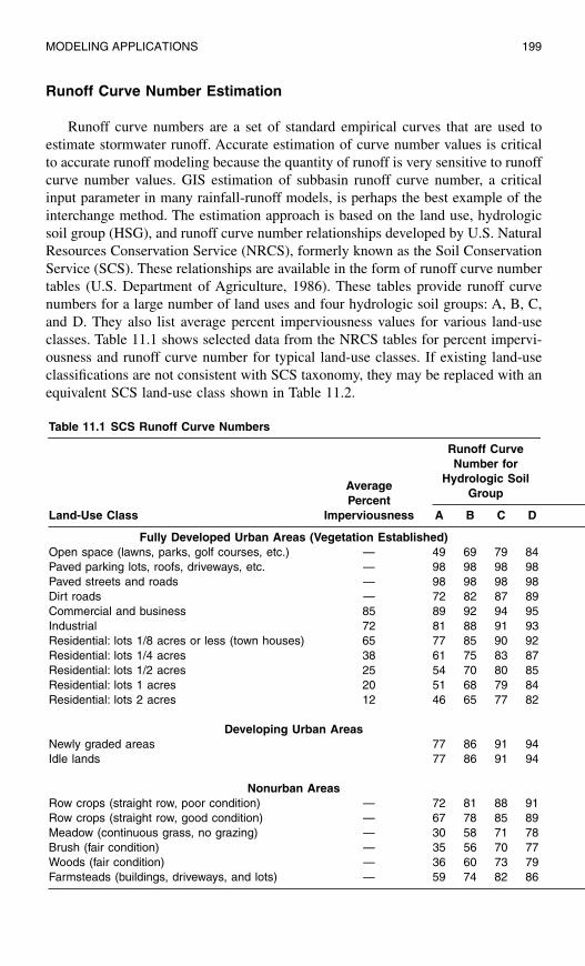
MODELING APPLICATIONS 199
Runoff Curve Number Estimation
Runoff curve numbers are a set of standard empirical curves that are used toestimate stormwater runoff. Accurate estimation of curve number values is criticalto accurate runoff modeling because the quantity of runoff is very sensitive to runoffcurve number values. GIS estimation of subbasin runoff curve number, a criticalinput parameter in many rainfall-runoff models, is perhaps the best example of theinterchange method. The estimation approach is based on the land use, hydrologicsoil group (HSG), and runoff curve number relationships developed by U.S. NaturalResources Conservation Service (NRCS), formerly known as the Soil ConservationService (SCS). These relationships are available in the form of runoff curve numbertables (U.S. Department of Agriculture, 1986). These tables provide runoff curvenumbers for a large number of land uses and four hydrologic soil groups: A, B, C,and D. They also list average percent imperviousness values for various land-useclasses. Table 11.1 shows selected data from the NRCS tables for percent impervi-ousness and runoff curve number for typical land-use classes. If existing land-useclassifications are not consistent with SCS taxonomy, they may be replaced with anequivalent SCS land-use class shown in Table 11.2.
Table 11.1 SCS Runoff Curve Numbers
Land-Use Class
AveragePercent
Imperviousness
Runoff CurveNumber for
Hydrologic SoilGroup
A B C D
Fully Developed Urban Areas (Vegetation Established)Open space (lawns, parks, golf courses, etc.) — 49 69 79 84Paved parking lots, roofs, driveways, etc. — 98 98 98 98Paved streets and roads — 98 98 98 98Dirt roads — 72 82 87 89Commercial and business 85 89 92 94 95Industrial 72 81 88 91 93Residential: lots 1/8 acres or less (town houses) 65 77 85 90 92Residential: lots 1/4 acres 38 61 75 83 87Residential: lots 1/2 acres 25 54 70 80 85Residential: lots 1 acres 20 51 68 79 84Residential: lots 2 acres 12 46 65 77 82
Developing Urban AreasNewly graded areas 77 86 91 94Idle lands 77 86 91 94
Nonurban AreasRow crops (straight row, poor condition) — 72 81 88 91Row crops (straight row, good condition) — 67 78 85 89Meadow (continuous grass, no grazing) — 30 58 71 78Brush (fair condition) — 35 56 70 77Woods (fair condition) — 36 60 73 79Farmsteads (buildings, driveways, and lots) — 59 74 82 86

200 GIS APPLICATIONS FOR WATER, WASTEWATER, AND STORMWATER SYSTEMS
A vector layer for subbasin runoff curve numbers is created by overlaying thelayers for subbasins, soils, and land use to delineate the runoff curve number polygons.Each resulting polygon should have at least three attributes: subbasin ID, land use,and HSG. The NRCS landuse-HSG-curve number matrix (Table 11.1 or Table 11.2)can now be used to assign runoff curve numbers to each polygon according to itsland use and HSG. Polygon runoff curve number values are then area-weighted tocompute the mean runoff curve number for each subbasin. These subbasin-runoffcurve numbers can now be entered into the model input file. The runoff curve numberestimation technique is shown in Figure 11.2 to Figure 11.5. Figure 11.2 shows thelayers for subbasins and land use. Figure 11.3 shows the layers for subbasins andHSGs. Figure 11.4 shows the computed runoff curve number polygons. Figure 11.5shows the average runoff curve numbers for the subbasins.
Some H&H models also need an input for the subbasin percent imperviousness,which can be estimated in GIS using the NRCS runoff curve number tables. A layerfor the subbasin percent imperviousness can be created by overlaying the layers forsubbasins and land use to delineate the percent imperviousness polygons. The land-use percent imperviousness matrix can then be used to assign percent imperviousvalues to the polygons. Finally, polygon percent imperviousness values are area-weighted to compute the mean percent imperviousness value for each subbasin.
Water Quality Modeling Data Estimation
Some urban-runoff quality models such as the TRANSPORT Block of SWMMneed curb length as a model input parameter, which can be estimated from a GISlayer of road or street centerlines. Subbasin curb length can be estimated by performing
Table 11.2 Equivalent SCS Land-Use Classes
Land-Use ClassSCS Equivalent Land-Use Class
Average Percent
Imperviousness
Runoff CurveNumber for
Hydrologic SoilGroup
A B C D
Parks, cemeteries,ball fields, etc.
Open space 0 39 61 74 80
High-density residential Average lot506–1012 m2
(0.125–0.25 acres)
51 69 80 87 90
Medium-density residential Average lot1349–2024 m2
(1/3–1/2 acres)
28 56 71 81 86
Low-density residential Average lot4047–8094 m2
(1–2 acres)
16 49 66 78 83
Schools Average lot1349–2024 m2
(1/3–1/2 acres)
28 56 71 81 86
Agricultural Row crops average 0 64 75 83 87Disturbed Newly graded areas 35 77 86 91 94

MODELING APPLICATIONS 201
an overlay analysis of street and subbasin layers. For example, in ArcView 3.x, curblength can be estimated by performing a theme-on-theme selection using roads as thetarget theme and subbasins as the selector theme. Alternatively, for large areas suchtasks can be handled more efficiently in ArcView’s Network Analyst extension, whichhas been designed for transportation network applications. Network Analyst is anoptional extension that must be purchased separately.
Figure 11.2 Layers for subbasins and land use for runoff curve number estimation.
Figure 11.3 Layers for subbasins and HSGs for runoff curve number estimation.

202 GIS APPLICATIONS FOR WATER, WASTEWATER, AND STORMWATER SYSTEMS
Demographic Data Estimation
Demographic data can be used for the following modeling tasks:
1. Estimation of quantity and quality sanitary sewage flow2. Estimation of present and potential future development3. Creation of auxiliary layers for visualization and presentation purposes
Figure 11.4 Computed runoff curve number polygons.
Figure 11.5 Subbasin runoff curve number map.
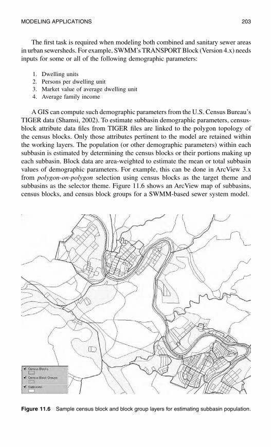
MODELING APPLICATIONS 203
The first task is required when modeling both combined and sanitary sewer areasin urban sewersheds. For example, SWMM’s TRANSPORT Block (Version 4.x) needsinputs for some or all of the following demographic parameters:
1. Dwelling units2. Persons per dwelling unit3. Market value of average dwelling unit4. Average family income
A GIS can compute such demographic parameters from the U.S. Census Bureau’sTIGER data (Shamsi, 2002). To estimate subbasin demographic parameters, census-block attribute data files from TIGER files are linked to the polygon topology ofthe census blocks. Only those attributes pertinent to the model are retained withinthe working layers. The population (or other demographic parameters) within eachsubbasin is estimated by determining the census blocks or their portions making upeach subbasin. Block data are area-weighted to estimate the mean or total subbasinvalues of demographic parameters. For example, this can be done in ArcView 3.xfrom polygon-on-polygon selection using census blocks as the target theme andsubbasins as the selector theme. Figure 11.6 shows an ArcView map of subbasins,census blocks, and census block groups for a SWMM-based sewer system model.
Figure 11.6 Sample census block and block group layers for estimating subbasin population.

204 GIS APPLICATIONS FOR WATER, WASTEWATER, AND STORMWATER SYSTEMS
Land-Use Data Estimation
Dry- and wet-weather flows from sewersheds depend on land use. Most rainfall-runoff models, therefore, need land-use information. In some models such as SWMM’sTRANSPORT Block, land-use type is input directly. In others, such as Penn StateRunoff Model (PSRM) and SWMM’s RUNOFF Block, land-use type is needed toderive certain model parameters such as percent imperviousness. TRANSPORT needsinput data for the the land-use designation of modeled subbasins. The subbasins shouldbe classified as having one of the five land-use classes:
1. Single-family residential2. Multifamily residential3. Commercial4. Industrial5. Open space
Most land-use maps and layers have more than these five land-use classes.However, this is not a problem in GIS because the existing classes can be easilyconsolidated into the five land-use classes mentioned above. Figure 11.7 shows anArcView 3.x screenshot for subbasin and land-use layers for a SWMM-based sewersystem model. The land-use layer was prepared from classification of 30-m-reso-lution Landsat Thematic Mapper (TM) satellite imagery of the study area. Initially,the layer contained 19 land-use classes. Subsequently, the initial land-use classes werereclassified into the five land-use types required for TRANSPORT input. In order torefine the land-use classification, the layer was combined with the census-block layer
Figure 11.7 Estimating land use using interchange method.

MODELING APPLICATIONS 205
to determine where population densities indicated residential districts. This was donein two ways. First, all nonresidential classed areas were examined to determine ifpopulation densities in the local census blocks were below or above a threshold often persons per acre. This threshold was chosen as a conservative breakpoint thatwould allow a reasonable portion of the classification to be correctly reclassified.The areas corresponding to any blocks with densities above the threshold werechanged to the residential class. Second, the census blocks of all residential areaswere examined to determine in which blocks single-family or multi-family residentialunits were the majority. On this basis polygons of the residential class were dividedinto single-family residential or multi-family residential classes.
INTERFACE METHOD
The interface method provides a direct link to transfer information between theGIS and a model. The interface method consists of at least the following twocomponents: (1) a preprocessor that analyzes and exports the GIS data to createmodel input files and (2) a postprocessor that imports the model output and displaysit as a GIS theme. Processing of the model input and output files requires computerprogramming using the GIS software’s scripting language (such as Avenue or VBA).User routines and scripts are incorporated in the GIS by calling them through newpull-down menus and icons.
The interface method basically automates the data interchange method. Theautomation is accomplished by adding model-specific menus or buttons to the GISsoftware. The model is executed independently of the GIS; however, the input fileis created in the GIS. The main difference between the interchange and interfacemethods is the automatic creation of the model input file. In the data interchangemethod, the user finds a portion of a file and copies it. In the interface method, aninterface automates this process, so that the pre- and postprocessor can find theappropriate portion of the file automatically.
Learning with examples is an effective method, so let us begin with an interfaceexample. Let us assume that we want to create an input file for a hydrologic modelby exporting GIS data to an ASCII text file. Our watershed GIS has the followingdata:
• Subbasins with attributes: ID, area, overland flow width, slope, and percent imper-viousness.
• Reaches (streams) with attributes: ID, upstream subbasin, downstream subbasin,type (natural stream, concrete channel, or concrete pipe), condition (best, good,fair, or bad), depth, width, length, upstream elevation, and downstream elevation.
Our hydrologic model requires a text file with the following input parameters:
• Subbasin data: ID, area, overland flow width, slope, and percent imperviousness.• Conduit data: ID, upstream subbasin, downstream subbasin, type, depth, width,
length, slope, and roughness coefficient.
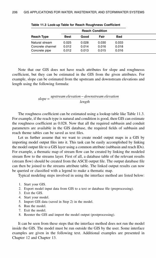
206 GIS APPLICATIONS FOR WATER, WASTEWATER, AND STORMWATER SYSTEMS
Note that our GIS does not have reach attributes for slope and roughnessscoefficient, but they can be estimated in the GIS from the given attributes. Forexample, slope can be estimated from the upstream and downstream elevations andlength using the following formula:
The roughness coefficient can be estimated using a lookup table like Table 11.3.For example, if the reach type is natural and condition is good, then GIS can estimatethe roughness coefficient as 0.028. Now that all the required subbasin and conduitparameters are available in the GIS database, the required fields of subbasin andreach theme tables can be saved as text files.
Let us further assume that we want to create model output maps in a GIS byimporting model output files into it. This task can be easily accomplished by linkingthe model output file to a GIS layer using a common attribute (subbasin and reach IDs).For example, a thematic map of stream flow can be created by linking the modeledstream flow to the streams layer. First of all, a database table of the relevant results(stream flow) should be created from the ASCII output file. The output database filecan then be joined to the streams attribute table. The linked output results can nowbe queried or classified with a legend to make a thematic map.
Typical modeling steps involved in using the interface method are listed below:
1. Start your GIS.2. Export model input data from GIS to a text or database file (preprocessing).3. Exit the GIS.4. Start your model.5. Import GIS data (saved in Step 2) in the model.6. Run the model.7. Exit the model.8. Reenter the GIS and import the model output (postprocessing).
It can be seen from these steps that the interface method does not run the modelinside the GIS. The model must be run outside the GIS by the user. Some interfaceexamples are given in the following text. Additional examples are presented inChapter 12 and Chapter 13.
Table 11.3 Look-up Table for Reach Roughness Coefficient
Reach Type
Reach Condition
Best Good Fair Bad
Natural stream 0.025 0.028 0.030 0.033Concrete channel 0.012 0.014 0.016 0.018Concrete pipe 0.012 0.013 0.015 0.016
slopeupstream elevation downstream elevation
length= −

MODELING APPLICATIONS 207
HEC-GEO Interface
The Hydrologic Engineering Center (HEC) is an office of the U.S. Army Corpsof Engineers (COE) established to support the nation’s hydrologic engineering andwater resources planning and management needs. To accomplish this goal, HECdevelops state-of-the-art, comprehensive computer programs that are also availableto the public. HEC-1 and HEC-2 are COE’s legacy DOS programs for hydrologicand hydraulic modeling, respectively. Recently HEC-1 and HEC-2 have beenreplaced with Windows programs called the Hydrologic Modeling System (HEC-HMS) and River Analysis System (HEC-RAS), respectively. HEC Geo-HMS andHEC Geo-RAS have been developed as geospatial hydrology toolkits for HEC-HMSand HEC-RAS users, respectively. They allow users to expediently create hydrologicinput data for HEC-HMS and HEC-RAS models. Free downloads of these programsare available from the HEC software Web site.
HEC-GeoHMS
HEC-GeoHMS is an ArcView 3.x GIS extension specifically designed to processgeospatial data for use with HEC-HMS. It allows users to visualize spatial infor-mation, delineate watersheds and streams, extract physical watershed and streamcharacteristics, perform spatial analyses, and create HEC-HMS model input files.HEC-GeoHMS uses ArcView’s Spatial Analyst Extension to develop a number ofhydrologic modeling inputs. Analyzing digital terrain information, HEC-GeoHMStransforms drainage paths and watershed boundaries into a hydrologic data structurethat represents watershed’s response to precipitation. In addition to the hydrologicdata structure, capabilities include the development of grid-based data for linearquasi-distributed runoff transformation (ModClark), the HEC-HMS basin model,and the background map file.
HEC-GeoHMS provides an integrated work environment with data managementand customized toolkit capabilities, which includes a graphical user interface (GUI)with menus, tools, and buttons. The program features terrain-preprocessing capabil-ities in both interactive and batch modes. Additional interactive capabilities allowusers to construct a hydrologic schematic of the watershed at stream gauges, hydrau-lic structures, and other control points. The hydrologic results from HEC-GeoHMSare then imported by HEC-HMS, where simulation is performed. HEC-GeoHMSworks with Windows 95/98/NT/2000 operating systems.
HEC-GeoRAS
HEC-GeoRAS (formerly named AV/RAS) for ArcView is an ArcView 3.x GISextension specifically designed to process geospatial data for use with HEC-RAS.The extension allows users to create an HEC-RAS import file containing geometricattribute data from an existing digital terrain model (DTM) and complementary datasets. HEC-GeoRAS automates the extraction of spatial parameters for HEC-RASinput, primarily the 3D stream network and the 3D cross-section definition. Resultsexported from HEC-RAS may also be processed in HEC-GeoRAS. ArcView 3D

208 GIS APPLICATIONS FOR WATER, WASTEWATER, AND STORMWATER SYSTEMS
Analyst extension is required to use HEC-GeoRAS. Spatial Analyst is recommended.An ArcInfo 7.x version of HEC-GeoRAS is also available.
Haestad Methods’ HEC-GIS system combines COE’s HEC-RAS floodplainmodeling program with ArcInfo. HEC-GIS is an Arc Macro Language (AML)program that allows importing floodplain cross-section data from a DEM withinArcInfo, in the form of triangular irregular networks (TINs). It also allows importingHEC-RAS water surface profiles back into HEC-GIS to perform additional spatialanalyses and mapping.
Watershed Modeling System
Watershed Modeling System (WMS) is a comprehensive hydrologic modelingpackage developed by the Environmental Modeling Research Laboratory (EMRL)of Brigham Young University in cooperation with the U.S. Army COE WaterwaysExperiment Station (WES) (WMS, 2000; Nelson et al., 1993). The focus of WMSis to provide a single application that integrates digital terrain models with industry-standard lumped-parameter hydrologic models such as HEC-1 and TR-20. In thisway, hydrologic data developed in ArcInfo, ArcView, or WMS can be directly linkedto many common hydrologic models. WMS includes an interface to HEC-1, TR-20,and the Rational Method programs used by many hydrologic engineers to modelthe rainfall-runoff process.
WMS can import and export GIS data. WMS’ GIS interface is accomplishedthrough its map module. Map module data is structured after ArcInfo 7.x, whichmakes it easy to import and use vector data created inside ArcInfo or any other GISthat can export an ArcInfo GENERATE file. WMS includes an ArcView 3.x exten-sion that facilitates the movement of data from GIS to WMS for hydrologic modeldevelopment. The interface allows for automatic development of a topological modelfrom TINs. Furthermore, any geometric parameters computed by WMS are suppliedto the corresponding model input fields. The extension preprocesses the GIS datato export hydrologic modeling data. WMS then reads a single file (describing therelevant themes exported) to obtain data from the GIS. These data can then be usedin WMS to create an initial model for any of the hydrologic programs supported byWMS. WMS itself is integrated with the hydrologic models. Data entry for thehydrologic model — including rainfall, job control, or any other parameters notdefined as attributes in GIS Shapefiles — can be completed using WMS’ hydrologicmodeling interface. WMS can be used to postprocess and then import model resultsin the GIS software. A screenshot of the WMS interface is shown in Figure 11.8.Unlike some HEC programs such as HEC-HMS and HEC-RAS, WMS is not free.A demo version can be downloaded from the BYU Web site.
GISHydro Modules
GISHydro is a collection of programs, demos, exercises, data, reports, andinformation designed to support the use of GIS in hydrology and water resourcesstudies. These materials are mostly drawn from the work of Professor David R.Maidment and a community of his graduate students, research scientists, and faculty

MODELING APPLICATIONS 209
in the Center for Research in Water Resources (CRWR) and the Department of CivilEngineering of the University of Texas at Austin. Initially, CRWR developed aprototype Spatial Hydrology Analysis System (Maidment, 1997) consisting of eightGISHydro modules. These modules, more than just computer programs, are a meth-odological approach to solving specific types of hydrologic problems using GIS.They contain ArcView and ArcInfo extensions, Avenue and AML scripts, sampledata, user instructions, and example exercises. Two GISHydro modules are describedin the following subsections:
GISHydro Prepro
This module is a procedure for connecting GIS to external models. Consistingof Avenue and AML scripts, it is designed to transform a subbasins-and-streamsnetwork into a schematic model of the hydrologic elements of a watershed. It wasinitially developed as a preprocessor for COE’s new Hydrologic Modeling System(HEC-HMS), which replaced the old HEC-1 model. GH-Prepro takes stream andsubbasin GIS data layers and analyzes them to produce a schematic model that
Figure 11.8 WMS interface.

210 GIS APPLICATIONS FOR WATER, WASTEWATER, AND STORMWATER SYSTEMS
defines and spatially connects seven types of hydrologic elements in the landscape:subbasins, reaches, junctions, diversions, reservoirs, sources, and sinks.
GISHydro Runoff
This module provides articles, reports, exercises, and a sample ArcView 3.xextension to compute watershed parameters and runoff at the outlet of a watershed.The ArcView extension uses the Texas Department of Transportation (TxDOT) state-wide regional rural regression equations for estimating stormwater runoff. Figure 11.9shows a screenshot of the TxDOT extension (Olivera and Bao, 1997).
ArcInfo Interface with HEC Programs
Another example of the interface method is the ArcInfo and HEC-1 and HEC-2interface developed by Woolpert, Inc. (Phipps, 1995). In HEC-1, the interface modeluses vector layers for streams and open channels and the ArcInfo networking functionto show the locations of and the relationships between different types of flows: sheetflow, shallow channel flow, and concentrated channel flow. The ArcInfo and HEC-1
Figure 11.9 GISHydro TxDOT extension.

MODELING APPLICATIONS 211
linkage allows users to see graphically, on a map, how fast the three flow types aremoving at different locations within the model (volume/time). The unit hydrographsgenerated in the HEC-1 hydrologic model are then used to feed the HEC-2 hydraulicmodel. The ArcInfo and HEC-2 interface allows graphical display of the 2-, 10-,25-, 50-, 100-, and 500-year frequency flood profiles for the streams and openchannels within the watershed. It was found that this interface allowed for easiermodel development and calibration, which resulted in substantial savings in the costof modeling tasks.
Intermediate Data Management Programs
Some commercial modeling products use an intermediate data managementprogram to facilitate data transfer between the GIS and a model. This program iswritten specifically to import data from a variety of common third-party GIS softwareand export data to a model data set. Under certain conditions this approach couldbe defined as an interface, but generally it is not. In relation to the Shamsi taxonomy,this method lies between the interchange and interface methods (Heaney et al., 1999).Haestad Methods’ GIS connection wizards for the company’s WaterCAD, Sewer-CAD, and StormCAD programs (described elsewhere in this book) are typicalexamples of this method. Figure 11.10 shows WaterCAD’s Import Shapefile wizard,
Figure 11.10 WaterCAD’s Import Shapefile wizard.

212 GIS APPLICATIONS FOR WATER, WASTEWATER, AND STORMWATER SYSTEMS
which is used to import WaterCAD model input parameters from ArcView GISShapefiles.
Interface Method Case Study
Very often, the software required to solve complex hydrologic problems is avail-able only in separate pieces rather than as an integrated package. Simulation modelsand GIS and SVS packages are individually strong in specific aspects of spatialanalysis but inadequate in cross-functional analysis of complex hydrologic problems.An integrated system consisting of a hydroclimatic simulation model (Rhea), a GIS(ArcInfo), and an SVS (DX) was developed to facilitate model development, cali-bration, and verification and visual representations of precipitation across space andtime. AML tools translated ArcInfo data into a format that could be read by DX. Theconverted DX file was used to generate animated, interactive displays using DXsoftware. The integrated system provided improved understanding of hydroclimaticprocesses in mountainous regions. An additional benefit of the integrated system, thevalue of which is often underestimated, is the improved ability to communicate modelresults (Hay and Knapp, 1996).
INTEGRATION METHOD
In the interface method, options for data editing and launching the model fromwithin the GIS software are not available. An interface simply adds new menus orbuttons to a GIS to automate the transfer of data between a computer model and aGIS. GIS integration, on the other hand, is a combination of a model and a GISsuch that the combined program offers both GIS and modeling functions. Thismethod represents the closest relationship between a GIS and a model. Two inte-gration approaches are possible:
1. GIS-based integration: In this approach, modeling modules are developed in orare called from within a GIS. All the four tasks of creating model input, editing
GIS software ArcInfoModeling software Rhea, an orographic precipitation model developed at the
Colorado State University (Rhea, 1977). The Rhea model simulates the interaction of air layers with underlying topography by allowing vertical displacement of the air column while keeping track of the resulting condensate or evaporation.
Other software Data Explorer (DX), a Scientific Visualization System (SVS) software from IBM
GIS data DEM grid, city locations, rivers, and rain-gauge locationsGIS format Raster and vectorStudy area 20,530 km2 Gunnison River Basin in southwestern ColoradoOrganization U.S. Geological Survey

MODELING APPLICATIONS 213
data, running the model, and displaying output results are available in the GIS.There is no need to exit the GIS to edit the data file or run the model. Becausedevelopment and customization tools within most GISs provide relatively simpleprogramming capability, this approach provides limited modeling power. It offersfull GIS functionality and simplistic modeling capability. It is often more popularbecause of the availability of computer code for a large number of public-domainlegacy computer models, such as SWMM and EPANET, which can be easilycustomized for GIS integration.
2. Model-based integration: In this method, GIS modules are developed in or arecalled from a computer model. It provides GIS-like functionality to computermodels. Because it is difficult to program all the GIS functions into a computermodel, this approach provides limited GIS capability. In this method, GIS isessentially used as a mapping tool. Sophisticated data management and datavisualization capabilities are not present. PCSWMM GIS [described in Chapter 13(Sewer Models)] and Runoff97 (Ritter and Gallie, 1998) are examples of themodel-based integration method. In this method, GIS and models are integratedthrough a common interface that requires extensive computer programming usingconventional computer languages (e.g., FORTRAN), and/or GIS macro and script-ing languages (e.g., AML, Avenue or VBA).
Representative examples of the integration method are given in the followingsubsections.
EPA’s BASINS Program
EPA’s BASINS program is the best example of GIS integration with multiple models.
The best example of GIS integration with multiple models is the BetterAssessment Science Integrating Point and Nonpoint Sources (BASINS) program.Originally released in September 1996, BASINS was developed by TetraTech,Inc., for the U.S. Environmental Protection Agency (EPA). BASINS supports thedevelopment of total maximum daily loads (TMDLs) using a watershed-basedapproach that integrates both point and nonpoint sources. BASINS integratesArcView 3.x GIS with national watershed data and state-of-the-art environmentalassessment and modeling tools into one convenient package. The heart of BASINSis its suite of interrelated components essential for performing watershed andwater quality analysis. These components are grouped into the following fivecategories:
1. National databases2. Assessment tools for evaluating water quality and point source loadings at a variety
of scales3. Utilities, such as land-use and DEM reclassification and watershed delineation4. Watershed and water quality models including NPSM, TOXIROUTE, and
QUAL2E5. Postprocessing output tools for interpreting model results

214 GIS APPLICATIONS FOR WATER, WASTEWATER, AND STORMWATER SYSTEMS
What Is TMDL?
According to EPA, TMDL is defined as “a calculation of the maximum amount of apollutant that a water body can receive and still meet water quality standards, and theallocation of that amount to the pollutant’s sources.” Technically, TMDL can be definedwith the help of the following equation:
TMDL
= WLAP
+ LAN
+ RC
+ FOS
where:WLAP
= waste load allocations for point sourcesLAN
= load allocations for nonpoint sourcesRC
= reserve capacity for future growthFOS
= factor of safety
BASINS integrates three models within an ArcView GIS environment: NPSM(HSPF), TOXIROUTE, and QUAL2E. Nonpoint Source Model (NPSM) estimatesland-use-specific NPS loadings for selected pollutants at a watershed (catalogingunit or user-defined subwatershed) scale. The model uses landscape data such aswatershed boundaries and land-use distribution to automatically prepare many ofthe required input data parameters. NPSM combines a Windows-based interface withEPA’s HSPF and is linked to ArcView. HSPF is a model for developing NPS loadsand is the backbone of the BASINS modeling system. TOXIROUTE is a screening-level stream-routing model that performs simple dilution and decay calculationsunder mean- or low-flow conditions for a stream system. QUAL2E is a one-dimen-sional, steady-state water quality and eutrophication model. It is integrated withArcView through a Windows-based interface. It allows fate and transport modelingfor both point and nonpoint sources. Both TOXIROUTE and QUAL2E can use NPSloadings calculated by HSPF.
Overcoming the lack of integration, limited coordination, and time-intensive exe-cution typical of more traditional assessment tools, BASINS makes watershed andwater quality studies easier by bringing key data and analytical components togetherunder one roof. The simulation models run in a Windows environment using data inputfiles generated in ArcView. By using GIS, a user can visualize, explore, and query tobring a watershed to life. This allows the user to assess watershed loadings andreceiving-water impacts at various levels of complexity. ArcView geographic datapreparation, selection routines, and visual output streamline the use of the models. Apostprocessor graphically displays model results. Figure 11.11 shows a screenshot ofthe BASINS program showing an example of delineated watersheds.
BASINS is distributed on a CD-ROM containing the BASINS program and datafor an EPA region of interest. It can also be downloaded from the BASINS Website. BASINS Version 1.0 was released in September 1996 (Lahlou, et al., 1996) forArcView Version 2.1. BASINS Version 2.0 was released in December 1998 forArcView 3.0. It included a national data set on the attributes listed in Table 11.4(Battin et al., 1998). BASINS Version 3.0 was released in 2001 for ArcView 3.2.

MODELING APPLICATIONS 215
Figure 11.11 BASINS screenshot showing an example of delineated watersheds.
Table 11.4 BASINS Database Attributes
Spatially Distributed DataLand use/land cover USGS hydrologic unit boundariesUrbanized areas Drinking water suppliesPopulated place location Dam sitesReach File, Version 1 (RF1) EPA region boundariesReach File, Version 3 (RF3) State boundariesSoils (STATSGO) County boundariesElevation (DEM) Federal and Indian landsMajor roads Ecoregions
Environmental Monitoring DataWater quality monitoring station summaries USGS gauging stationsWater quality observation data Fish and wildlife advisoriesBacteria monitoring station summaries National Sediment Inventory (NSI)Weather station sites (477) Shellfish contamination inventoryClean water needs survey —
Point-Source DataPermit compliance system Industrial Facilities Discharge (IFD) sitesToxic Release Inventory (TRI) sitesMineral availability system/mineral industry location
Superfund national priority list sitesResource Conservation and Recovery Act (RCRA) sites

216 GIS APPLICATIONS FOR WATER, WASTEWATER, AND STORMWATER SYSTEMS
BASINS 2.0 included a watershed delineation tool, a land-use reclassification tool,an HSPF interface, a watershed characterization report on STORET water quality data,DEM elevation data, and USEPA Reach File Version 3 Alpha (RF3 Alpha). Using theimport tool, users can add their own data for watershed boundaries, streams, elevation,land use, and observed water quality into the BASINS system. Using the land-usereclassification tool, users can reclassify part of the land-use theme or the entire themeinteractively to create more detailed levels of land use. This feature can be used tostudy the potential impact of land-use changes on water quality. The watershed-delineation tool allows users to interactively subdivide a USGS 8-digit watershed intosmaller subwatersheds using mouse point-and-click inputs. Subdelineated watershedsand underlying data are then available for more detailed modeling.
BASINS 3.0 is the latest (year 2001) release at the time of this writing. Thisrelease includes additional functional capabilities as well as an updated and expandedset of national data layers. New data and functions include 1
° DEM grids, an auto-matic delineation tool that creates watershed boundaries based on DEM grids, and anew watershed report function for land use, topography, and hydrologic responseunits. In addition, a new watershed model, the Soil and Water Assessment Tool(SWAT), has been added. SWAT is a watershed-scale model developed to predict theimpact of land management practices on water, sediment, and agricultural chemicalyields in large complex watersheds with varying soils, land use, and managementconditions over long periods of time.
BASINS 3.0 also demonstrates an important change in the development philos-ophy of BASINS. It is distributed as a core system with several ArcView extensions.All BASINS data management utilities, assessment tools, report tools, and modelswere converted as extensions. This modular and open architecture offers numerousadvantages both to users and developers. For instance, users may customize theirBASINS project to include only extensions that are needed. Moreover, it will beeasier for developers to maintain and provide updates of individual extensionsbecause it will not involve changing and reissuing a patch or new version for theentire system. This makes it easier for users to upgrade their system. It also encour-ages the development of extensions for BASINS by users and developers.
BASINS 3.0 installation software contains the new BASINS Version 3.0 systemand the tutorial data set (HUC-05010007). In addition to BASINS 3.0, the installationprogram installs WinHSPF, GenScn, WDMUtil, and PLOAD. WinHSPF is a newinterface to HSPF Version 12, which is replacing NPSM from BASINS 2.0. GenScnis a model postprocessing and scenario-analysis tool that is used to analyze outputfrom HSPF and SWAT. WDMUtil is used to manage and create watershed datamanagement files (WDMs) that contain the meteorological data and other time-seriesdata used by HSPF. PLOAD is a GIS and spreadsheet tool to calculate nonpointsources of pollution in watersheds.
EPA plans to release an update (Version 3.1) in 2004 on the existing ArcView 3.xplatform. EPA is currently working on pieces of BASINS for the ArcGIS environment.After the BASINS 3.1 release, EPA plans to port it onto the ArcGIS platform based onthe work done by the Center for Research in Water Resources at the University of Texasat Austin, Water Resources Consortium, and ESRI. Future releases of BASINS mayinclude EPA’s SWMM program, automatic model calibration, and a reach-indexing tool

MODELING APPLICATIONS 217
for georeferencing. A redesign of the BASINS system using RDBMS, Internet, MapOb-jects, and Java technologies is also anticipated. This move toward a more fully integratedGIS and database system will provide many more BASINS applications. The watershedtool will evolve into a more component-based architecture, so that users will need toinstall only the components required for their specific analytical needs, including theirown legacy models (Whittemore and Beebe, 2000).
BASINS is a valuable tool that integrates environmental data, analytical tools,and modeling programs to support the development of cost-effective approaches toenvironmental protection. However, BASINS’ seamless integration power is notwithout some disadvantages. BASINS’ simplistic modeling approach and user-friendly tools may encourage inexperienced users to become instant modelers, whichcould be undesirable. The inexperienced users’ overreliance on default model seg-mentation and model coefficients, without an understanding of the underlyingassumptions, may result in inaccurate and unrealistic TMDLs (Thuman and Mooney,2000). BASINS builds upon federal databases of water quality conditions and point-source loadings for numerous parameters where quality assurance is suspect in somecases (Whittemore and Beebe, 2000).
BASINS Examples
Most of the BASINS work and modeling have been on a watershed- or regional-level scale. An example for the BASINS data set for Boulder, Colorado, is shownin Figure 11.12. The size of this file relative to the area it represents reflects a scale
Figure 11.12 BASINS GIS layers for Boulder, Colorado.

218 GIS APPLICATIONS FOR WATER, WASTEWATER, AND STORMWATER SYSTEMS
of about 1:2000 (Heaney et al., 1999). The Columbus Water Works of Columbus,Georgia, developed a BASINS 2 model for the 2400 mi2 (3600 km2) Middle Chat-tahoochee River Watershed. The main objectives of the model were to formulateTMDL allocation requirements of the Clean Water Act and to demonstrate compli-ance with EPA’s National Combined Sewer Overflow (CSO) Policy. They usedmonitoring and data management methodologies to calibrate their BASINS modeland to perform source-water assessments and protection through provisions of early-warning systems for drinking-water intake operations (Turner et al., 2000).
MIKE BASIN
Danish Hydraulic Institute’s (DHI) MIKE BASIN is an ArcView-based decisionsupport system for water resources planning and management. It serves as a gener-alized river basin network simulation modeling system for regional water resourcesallocation of complex systems. MIKE BASIN can be used to analyze water supplycapabilities in connection with water rights for municipal and industrial water supply,irrigation, and many multipurpose reservoir operations.
MIKE BASIN is fully integrated into ArcView 3.x. It uses a graphical userinterface, which links MIKE BASIN to ArcView. It is developed using the object-oriented C++ programming language, which allows for easy implementation of newfeatures. MIKE BASIN permits on-screen creation of models using image themesas backdrops. Figure 11.13 shows the MIKE BASIN interface.
Figure 11.13 MIKE BASIN screenshot.

MODELING APPLICATIONS 219
An important advantage of MIKE BASIN is its vertical compatibility with otherDHI modeling systems, which allows the use of several modeling tools of variouscomplexities at different stages of a project cycle. MIKE BASIN can be used inconjunction with other DHI models when detailed studies of specific problems arerequired. For example, MIKE SHE can be used for modeling runoff quality andquantity, including interaction with surface water systems, MIKE 11 can be usedfor detailed modeling of river hydrodynamics and water quality, and MIKE 21 canbe used for modeling bays and estuaries.
Geo-STORM Integration
An early example of ArcInfo 7.x and modeling integration is the Geo-STORMpackage developed by Innovative System Developers, Inc., Columbia, Maryland.Geo-STORM computed subbasin runoff, performed flow routing through reach andreservoir networks, and analyzed river hydraulics using SCS Technical Release 20(TR-20) and Technical Release 55 (TR-55) programs, and COE’s HEC-2 computerprograms. All these models were contained within a GUI environment within ArcInfoGIS. The software was written in AML, the ArcInfo scripting language. There wereexternal calls to the operating system only to execute the computer programs. Thecommon interface provided easy interaction between the models and switchingbetween the models was hardly noticeable, and output from one model was used asinput for another model. The TR-55 model was embedded within the TR-20 model.The output from TR-55 became input for TR-20. The TR-20 model provided dis-charge values for input to the HEC-2 model, and output from HEC-2 could bedirectly inserted into TR-20 as rating-table information. All modeling applicationswere integrated in Geo-GUIDE, a graphical interface that made working withArcInfo easier. The computer models were embedded within Geo-GUIDE, whichprovided plotting, reporting, and querying capabilities for the stormwater modelingsoftware suite. The GeoSTORM system was considered to be a database repositoryfor stormwater-related geography and facilities. Using programs like Geo-STORMtranslated into productivity gains realized by eliminating tedious tasks such asmanual map measurements, data entry, and tabular-report interpretation. Geo-STORM automated these time-consuming processes, drawing model inputs fromthe GIS database. This in time improved the quality and accuracy of model results.Figure 11.14 shows a screenshot of Geo-STORM (Thomas, 1995).
ARC/HEC-2 Integration
ARC/HEC-2 was one of the earliest integrations of ArcInfo and HEC-2, developedat the University of Texas at Austin. ARC/HEC-2 facilitated floodplain analysis in aGIS environment. It allowed direct usage of ArcInfo coverages for development ofHEC-2 input, running HEC-2 from within ArcInfo, and for conversion of HEC-2 water-surface elevations computed at each cross section into an ArcInfo coverage represent-ing the floodplain. There were two main data requirements for ARC/HEC-2 to operate:(1) a terrain representation in the form of constructed TIN or contours, and (2) channelcenterline (thalweg). ARC/HEC-2 consisted of three separate modules: preprocessor,

220 GIS APPLICATIONS FOR WATER, WASTEWATER, AND STORMWATER SYSTEMS
postprocessor, and viewer. The preprocessor created a complete HEC-2 input file readyto run. For complex HEC-2 models, manual editing of the input file was required, inwhich case ARC/HEC-2 served as an interface rather than an integration. The post-processor used the HEC-2 output to determine water surface elevation at each crosssection and, based on that information, found the outline of the flooded area in theform of a lattice and a polygon layer. This lattice and coverage could be used in ArcInfowith all other pertinent coverages for the area. Viewer was an AML application thatallowed viewing of the main input and output coverages in 2D and 3D formats (Djokicet al., 1993).
Integration Method Case Study
Successful implementation of environmental modeling databases involves theintegration of GIS, remote sensing, multiple databases, and visualization tools for
Figure 11.14 Geo-STORM screenshot showing ArcInfo and TR-20 integration.
GIS software ArcView and Spatial Analyst ExtensionModeling Software Agricultural Nonpoint Source Pollution Model (AGNPS)GIS data Soil (STATSGO), USGS DEM (1:250,000 scale), land
use, hydrography, watersheds, and crop managementStudy area 280 mi2 (810 km2) Dowagiac River Watershed located
in southwestern MichiganOrganization Western Michigan University, Kalamazoo, Michigan

MODELING APPLICATIONS 221
extraction of the needed model input parameters and for analysis and visualization ofthe simulated results. Although it was obvious that GIS technology was ideally suitedto accomplish these goals, current GIS packages were found to be difficult to use andoffered limited functions to support environmental modeling. It was also noted thatin current practice, GIS and hydrologic models were just used together, not reallyintegrated. Therefore, a custom interface called ArcView Nonpoint Source PollutionModeling (AVNPSM) was developed between ArcView GIS and AGNPS in supportof agricultural watershed analysis and nonpoint source pollution management.
AGNPS (Version 5.0) is a single storm event based simulation model for eval-uating sediment and nutrient (nitrogen, phosphorus, and chemical oxygen demandor COD) transport from agricultural watersheds. It represents the landscape of awatershed by discretizing the study area into individual grid cells. The PC Windows-based interface developed using Avenue scripts and Dialogue Designer consists ofseven modules: the AGNPS utility, parameter generator, input file processor, modelexecutor, output visualizer, statistical analyzer, and land-use simulator. Each moduleis incorporated into ArcView through pull-down menus and icons. The input fileprocessor menu produces an input file that is compatible with AGNPS input formatrequirements. The AGNPS model is executed either within Windows using the modelexecutor menu or run separately in simulated DOS mode. The output visualizermenu shows the simulated results of hydrology, sediment, and nutrients in tabularor map format. The calibrated model indicated that development of about 1240 acresof nonurban land caused little increase in the peak flow rate and sediment yield atthe mouth of the river and had almost no impact on the runoff volume and nutrientyields. The case study concluded that integration of GIS and simulation modelsfacilitates the development and application of environmental simulation models andenhances the capabilities of GIS packages (He et al., 2001).
WHICH LINKAGE METHOD TO USE?
Each method has its pros and cons. Table 11.5 lists the advantages and disad-vantages of the three methods of linking H&H models with GIS. Integrated systemsare easy to learn and use and make the excruciating task of H&H modeling a fun
Table 11.5 Comparison of GIS Linkage Methods
FeatureInterchange
MethodInterfaceMethod
IntegrationMethod
Automation Low Medium HighUser-friendliness None Medium HighEase of use Cumbersome Easy EasiestLearning curve Long Medium QuickData-entry error potential High Medium LowData-error tracking Easy Complex DifficultMisuse potential byinexperienced users
Low Medium High
Development effort Low Medium HighComputer programming Low Medium Extensive

222 GIS APPLICATIONS FOR WATER, WASTEWATER, AND STORMWATER SYSTEMS
activity. Integrated systems save model development and interpretation time andmake modeling cost-effective.
Seamless model integration with GIS is not without some disadvantages. Thesimplistic modeling approach and user-friendly tools provided by integrated systemslike BASINS may encourage inexperienced users to become instant modelers, whichcould be undesirable (Thuman and Mooney, 2000). GIS can easily convert reamsof computer output into colorful thematic maps that can both expose and hide dataerrors. The user-friendly interface of an integrated package may incorrectly make acomplex model appear quite simple, which may lead to misapplication of the modelby inexperienced users. Modeling should not be made easy at the expense of goodscience. Modeling, for all the new tools emerging in the 1990s, is still an art that isdone well by only a select few (Whittemore and Beebe, 2000).
The inexperienced users’ overreliance on default model parameters may resultin inaccurate modeling results. Inexperienced H&H modelers should exercise cautionwhen using integrated systems, make sure to browse the model input and outputfiles for obvious errors, and avoid overreliance on thematic mapping and graphingof model output. Modification and recompilation of computer codes of existinglegacy programs like SWMM or EPANET to create integrated systems should beavoided. If recoding is necessary, developers should be extremely cautious to avoidcoding errors and the associated liability. Users should remember that a difficult-to-use model is much better than an inaccurate model (Shamsi, 2001).
The development of a GIS for use in urban H&H modeling is an expensiveinvestment (Heaney et al., 1999). Typically the most advanced tools are created foradvanced applications, where a full-fledge GIS is in place. For some applications,a DOS-based model may still be the most appropriate. However, as more urban areascreate GIS layers, the integration of modeling software and GIS software willbecome more useful and prevalent.
USEFUL WEB SITES
CHAPTER SUMMARY
This chapter described GIS applications that have revolutionized the way H&Hmodeling is performed. It showed how GIS can be used to develop H&H models,and also provided a software review of GIS application programs. From the materialpresented in this chapter, it can be concluded that GIS applications allow modelersto be more productive. Users devote more time to understanding the problem andless time to mechanical tasks of data input and checking, getting the program to run,and interpreting reams of output. More than just tabular outputs, models become anautomated system evaluation tool. There are three modeling application methods:
HEC software www.hec.usace.army.mil/GIS Hydro www.crwr.utexas.edu/archive.shtmlBASINS software www.epa.gov/OST/BASINSWMS software http://emrl.byu.edu/wms.htm

MODELING APPLICATIONS 223
interchange, interface, and integration. Interchange is the simplest method but offerslimited benefits. Interchange systems have existed since 1980s in all domains. Theinterface method’s benefits lie between those of the interchange and the integrationmethods. There are a few interface systems in the public domain and many incommercial and proprietary domains. The integration method offers the maximumproductivity benefits. BASINS is the only public-domain modeling system that usesthe integration method. A few integrated commercial systems are available startingat $5000. There are many in-house and proprietary integrated systems. The numberof public-domain and commercial integration packages is expected to grow steadilyin the near future.
CHAPTER QUESTIONS
1. What are the GIS applications in computer modeling of water, wastewater, andstormwater systems?
2. What are computer modeling application methods?3. Give an example of each application method using programs other than those
described in this chapter.4. Which GIS application method is the easiest to use? Why?5. Which GIS application method is the easiest to implement? Why?6. List the typical steps used in the interface method.7. Make a list of the H&H models used in your organization and the type of GIS
application method used by each.


225
CHAPTER 12
Water Models
GIS saves time and money in developing water distribution systemhydraulic models for simulating flows and pressures in the system.GIS also helps in presenting the model results to non-technicalaudiences.
EPANET and ArcView GIS integration.
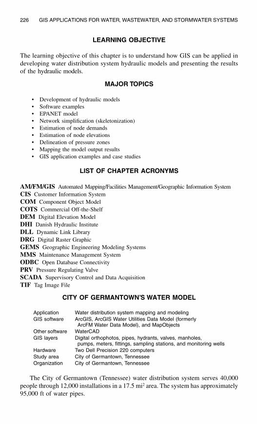
226 GIS APPLICATIONS FOR WATER, WASTEWATER, AND STORMWATER SYSTEMS
LEARNING OBJECTIVE
The learning objective of this chapter is to understand how GIS can be applied indeveloping water distribution system hydraulic models and presenting the resultsof the hydraulic models.
MAJOR TOPICS
• Development of hydraulic models• Software examples• EPANET model• Network simplification (skeletonization)• Estimation of node demands• Estimation of node elevations• Delineation of pressure zones• Mapping the model output results• GIS application examples and case studies
LIST OF CHAPTER ACRONYMS
AM/FM/GIS Automated Mapping/Facilities Management/Geographic Information SystemCIS Customer Information SystemCOM Component Object ModelCOTS Commercial Off-the-ShelfDEM Digital Elevation ModelDHI Danish Hydraulic InstituteDLL Dynamic Link LibraryDRG Digital Raster GraphicGEMS Geographic Engineering Modeling SystemsMMS Maintenance Management SystemODBC Open Database ConnectivityPRV Pressure Regulating ValveSCADA Supervisory Control and Data AcquisitionTIF Tag Image File
CITY OF GERMANTOWN’S WATER MODEL
The City of Germantown (Tennessee) water distribution system serves 40,000people through 12,000 installations in a 17.5 mi2 area. The system has approximately95,000 ft of water pipes.
Application Water distribution system mapping and modelingGIS software ArcGIS, ArcGIS Water Utilities Data Model (formerly
ArcFM Water Data Model), and MapObjectsOther software WaterCADGIS layers Digital orthophotos, pipes, hydrants, valves, manholes,
pumps, meters, fittings, sampling stations, and monitoring wellsHardware Two Dell Precision 220 computersStudy area City of Germantown, TennesseeOrganization City of Germantown, Tennessee

WATER MODELS 227
The City used ESRI’s geodatabase, an object-oriented GIS data model, to design adatabase. The database design was done with minimal customization of ESRI’s ArcGISWater Utilities Data Model. This approach helped complete the database design in afew weeks instead of several months. ESRI’s MapObjects was used to create a customutility tool set for developing the water distribution network. Valve and hydrant locationsfrom the digital orthophotos and planimetric mapping were used with the existing1 in.
=500 ft-scale paper map of the water system as the basis for connecting water pipes.
The GIS layers (Figure 12.1) were initially developed using the ArcView Shape-files. The Shapefiles were then migrated to a geodatabase. To ease the data migration,connectivity rules were stored in ArcCatalog rather than directly in the model.ArcMap “flag and solver” tracing tools were used to ensure topological integrity ofthe migrated data. ArcMap also provided the City with out-of-the-box networkanalysis functionality such as tracing paths and water main isolation.
For the development of the hydraulic model, the City did not have to create amodeling network from scratch. GIS was used to skeletonize the network for inputto the Haestad Method’s WaterCAD 4.1 hydraulic model. Spatial operations availablein ArcGIS were used to assign customer-demand data — obtained from the City’sbilling database and stored in parcel centroids — to modeling nodes. Node elevationswere extracted from the City’s DEM.
The hydraulic model was run to assess the future system expansion and capitalimprovement needs of the City. The model indicated that the system needed a newelevated storage tank and a larger pipe to deliver acceptable pressure under peakdemand conditions (ESRI, 2002b).
GIS APPLICATIONS FOR WATER DISTRIBUTION SYSTEMS
GIS has wide applicability for water distribution system studies. Representationand analysis of water-related phenomena by GIS facilitates their management. TheGIS applications that are of particular importance for water utilities include mapping,modeling, facilities management, work-order management, and short- and long-termplanning. Additional examples include (Shamsi, 2002):
• Conducting hydraulic modeling of water distribution systems.• Estimating node demands from land use, census data, or billing records.• Estimating node elevations from digital elevation model (DEM) data.• Performing model simplification or skeletonization for reducing the number of
nodes and links to be included in the hydraulic model.• Conducting a water main isolation trace to identify valves that must be closed to
isolate a broken water main for repair. Identifying dry pipes for locating customersor buildings that would not have any water due to a broken water main. Thisapplication is described in Chapter 15 (Maintenance Applications).
• Prepare work orders by clicking on features on a map. This application is describedin Chapter 14 (AM/FM/GIS Applications).
• Identifying valves and pumps that should be closed to isolate a contaminated partof the system due to acts of terrorism. Recommending a flushing strategy to cleanthe contaminated parts of the system. This application is described in Chapter 16(Security Planning Vulnerability Assessment).

228 GIS APPLICATIONS FOR WATER, WASTEWATER, AND STORMWATER SYSTEMS
• Providing the basis for investigating the occurrence of regulated contaminantsfor estimating the compliance cost or evaluating human health impacts (Schockand Clement, 1995).
• Investigating process changes for a water utility to determine the effectivenessof treatment methods such as corrosion control or chlorination.
• Assessing the feasibility and impact of system expansion.• Developing wellhead protection plans.
Figure 12.1 Germantown water distribution system layers in ArcGIS.

WATER MODELS 229
By using information obtained with these applications, a water system managercan develop a detailed capital improvement program or operations and maintenanceplan (Morgan and Polcari, 1991). The planning activities of a water distributionsystem can be greatly improved through the integration of these applications.
In this chapter, we will focus on the applications related to hydraulic modelingof water distribution systems.
DEVELOPMENT OF HYDRAULIC MODELS
The most common use of a water distribution system hydraulic model is to deter-mine pipe sizes for system improvement, expansion, and rehabilitation. Models are alsoused to assess water quality and age and investigate strategies for reducing detentiontime. Models also allow engineers to quickly assess the distribution network duringcritical periods such as treatment plant outages and major water main breaks.
Today, hydraulic models are also being used for vulnerability assessment and protectionagainst terrorist attacks.
Hydraulic models that are created to tackle a specific problem gather dust on a shelfuntil they are needed again years later. This requires a comprehensive and often expen-sive update of the model to reflect what has changed within the water system. A directconnection to a GIS database allows the model to always remain live and updated.
Denver Water Department, Colorado, installed one of the first AM/FM/GISsystems in the U.S. in 1986. In the early 1990s, the department installed the $60,000SWS water model from the Stoner Associates (now Advantica Stoner, Inc.). Aroundthe same time, Genesee County Division of Water and Waste Services in Flint,Michigan, started developing a countywide GIS database. The division envisionedcreating sewer and water layers on top of a base map and integrating the GIS layerswith their water and sewer models (Lang, 1992).
GIS applications reduce modeling development and analysis time. GIS can be usedto design optimal water distribution systems. An optimal design considers both cost-effectiveness and reliability (Quimpo and Shamsi, 1991; Shamsi, 2002a) simulta-neously. It minimizes the cost of the system while satisfying hydraulic criteria (accept-able flow and pressures). Taher and Labadie (1996) developed a prototype model foroptimal design of water distribution networks using GIS. They integrated GIS forspatial database management and analysis with optimization theory to develop a com-puter-aided decision support system called WADSOP (Water Distribution System Opti-mization Program). WADSOP employed a nonlinear programming technique as thenetwork solver, which offers certain advantages over conventional methods such asHardy-Cross, Newton Raphson, and linear system theory for balancing looped watersupply systems. WADSOP created a linkage between a GIS and the optimization model,which provided the ability to capture model input data; build network topology; verify,modify, and update spatial data; perform spatial analysis; and provide both hard-copyreporting and graphical display of model results. The GIS analysis was conducted inPC ARC/INFO. The ROUTE and ALLOCATE programs of the NETWORK module

230 GIS APPLICATIONS FOR WATER, WASTEWATER, AND STORMWATER SYSTEMS
of PC ARC/INFO were found to be very helpful. Computational time savings of 80to 99% were observed over the other programs.
Generally, there are four main tasks in GIS applications to water systemmodeling:
1. Synchronize the model’s network to match the GIS network.2. Transfer the model input data from a GIS to the model.3. Establish the model execution conditions and run the model.4. Transfer the model output results to GIS.
As described in Chapter 11 (Modeling Applications), GIS is extremely usefulin creating the input for hydraulic models and presenting the output. A hydraulicmodeler who spends hundreds of hours extracting input data from paper maps canaccomplish the same task with a few mouse clicks inside a GIS (provided that therequired data layers are available). GIS can be used to present hydraulic modelingresults in the form of thematic maps that are easy for nontechnical audiences tounderstand. Additional information about GIS integration methods is provided inChapter 11, which provided a taxonomy developed by Shamsi (1998, 1999) todefine the different ways a GIS can be linked to hydraulic models. According toShamsi’s classification, the three methods of developing GIS-based modeling appli-cations are interchange, interface, and integration. For GIS integration of waterdistribution system hydraulic models, one needs a hydraulic modeling softwarepackage. The software can run either inside or outside the GIS. As explained inChapter 11, when modeling software is run inside a GIS, it is considered “seam-lessly integrated” into the GIS. Most modeling programs run in stand-alone modeoutside the GIS, in which case the application software simply shares GIS data.This method of running applications is called a “GIS interface.”
The interchange method offers the most basic application of GIS in hydraulicmodeling of water distribution systems. In 1995, the Charlotte–MecklenburgUtility Department (CMUD) used this method to develop a KYPIPE model foran area serving 140,000 customers from 2,500 mi of water pipes ranging in sizefrom 2 in. to 54 in. (Stalford and Townsend, 1995). The modeling was startedby creating an AutoCAD drawing of all pipes 12 in. and larger. The pipes weredrawn as polylines and joined at the intersections. The AutoCAD drawing wasconverted to a facilities management database by placing nodes at the hydraulicintersections of the pipes, breaking the polylines as needed, adding extendedattributes to the polylines from the defined nodes, extracting this information intoexternal tables, and adding the nongraphical information to the tables. Then, byusing ArcCAD inside AutoCAD, coverages were created for the pipes and nodes,which could be viewed inside ArcView. Although this method was consideredstate-of-the-art in 1995, it is not a very efficient GIS integration method by today’sstandards. The EPANET integration case study presented later in the chapterexemplifies application of the more efficient integration method.
In the simplest application of the integration method, it should be possible to usea GIS to modify the configuration of the water distribution network, compile modelinput files reflecting those changes, run the hydraulic model from within the GIS, usethe GIS to map the model results, and graphically display the results of the simulation

WATER MODELS 231
on a georeferenced base map. The integration method interrelationships among theuser, the hydraulic model, and the GIS software are illustrated in Figure 12.2.
SOFTWARE EXAMPLES
Table 12.1 lists representative water distribution system modeling packages andtheir GIS capabilities, vendors, and Web sites. The salient GIS features of theseprograms are described in the following subsections.
EPANET
EPANET was developed by the Water Supply and Water Resources Division(formerly the Drinking Water Research Division) of the U.S. Environmental Pro-tection Agency’s National Risk Management Research Laboratory (Rossman,2000). It is a public-domain software that may be freely copied and distributed.
EPANET is a Windows 95/98/2K/NT program that performs extended-periodsimulation of hydraulic and water quality behavior within pressurized pipe networks.A network can consist of pipes, nodes (pipe junctions), pumps, valves, and storagetanks or reservoirs. EPANET tracks the flow of water in each pipe, the pressure ateach node, the height of water in each tank, and the concentration of a chemical species
Figure 12.2 Integration method interrelationships.

232 GIS APPLICATIONS FOR WATER, WASTEWATER, AND STORMWATER SYSTEMS
throughout the network during a simulation period made up of multiple time steps. Inaddition to chemical species, water age and source tracing can also be simulated.
The Windows version of EPANET provides an integrated environment for editingnetwork input data, running hydraulic and water quality simulations, and viewing theresults in a variety of formats. These include color-coded network maps, data tables,time-series graphs, and contour plots. Figure 12.3 shows an EPANET screenshot dis-playing pipes color-coded by head-loss and nodes color-coded by pressure.
The EPANET Programmer’s Toolkit is a dynamic link library (DLL) of functionsthat allow developers to customize EPANET’s computational engine for their ownspecific needs. The functions can be incorporated into 32-bit Windows applicationswritten in C/C++, Delphi Pascal, Visual Basic, or any other language that can callfunctions within a Windows DLL. There are over 50 functions that can be used to opena network description file, read and modify various network design and operatingparameters, run multiple extended-period simulations accessing results as they aregenerated or saving them to file, and write selected results to file in a user-specifiedformat. The toolkit should prove useful for developing specialized applications,such as optimization models or automated calibration models, that require runningmany network analyses while selected input parameters are iteratively modified.It also can simplify adding analysis capabilities to integrated network modeling envi-ronments based on CAD, GIS, and database management packages (Rossman, 2000a).
The current version of EPANET (Version 2.0) has neither a built-in GIS interface norintegration. Therefore, users must develop their own interfaces (or integration) or rely onthe interchange method to manually extract model input parameters from GIS data layers.
H2ONET™ and H2OMAP™
MWH Soft, Inc. (Broomfield, Colorado), provides infrastructure software andprofessional solutions for utilities, cities, municipalities, industries, and engineeringorganizations. The company was founded in 1996 as a subsidiary of the global
Table 12.1 Water Distribution System Modeling Software
Software Method Vendor Web site
EPANET Interchange U.S. Environmental Protection Agency(EPA)
www.epa.gov/ord/NRMRL/wswrd/epanet.html
AVWater Integration CEDRA Corporation www.cedra.comH2ONET andH2OMAP
Interface andIntegration
MWH Soft www.mwhsoft.com
InfoWorks WSand InfoNet
Interface andIntegration
Wallingford Software www.wallingfordsoftware.com
MIKE NET Interface DHI Water &Environment
www.dhisoftware.com
PIPE2000 Pro Interface University ofKentucky
www.kypipe.com
SynerGEE Water
Interface andIntegration
Advantica Stoner www.stoner.com
WaterCAD Interface Haestad Methods www.haestad.comWaterGEMS Integration

WATER MODELS 233
environmental engineering, design, construction, technology, and investment firmMWH Global, Inc. The company’s CAD- and GIS-enabled products are designedto manage, design, maintain, and operate efficient and reliable infrastructure systems.MWH Soft, provides the following water distribution system modeling software:
• H2ONET• H2OMAP Water• InfoWater• H2OVIEW Water
H2ONET is a fully integrated CAD framework for hydraulic modeling, networkoptimization, graphical editing, results presentation, database management, andenterprise-wide data sharing and exchange. It runs from inside AutoCAD and,therefore, requires AutoCAD installation.
Figure 12.3 EPANET screenshot (Harrisburg, Pennsylvania, model).

234 GIS APPLICATIONS FOR WATER, WASTEWATER, AND STORMWATER SYSTEMS
Built using the advanced object-oriented geospatial component model, H2OMAPWater provides a powerful and practical GIS platform for water utility solutions. Asa stand-alone GIS-based program, H2OMAP Water combines spatial analysis toolsand mapping functions with network modeling for infrastructure asset managementand business planning. H2OMAP Water supports geocoding and multiple mappinglayers that can be imported from one of many data sources including CAD drawings(e.g., DWG, DGN, and DXF) and standard GIS formats (Shapefiles, Generate files,MID/MIF files, and ArcInfo coverages). The program also supports the new geoda-tabase standard of ArcGIS through an ArcSDE connection.
InfoWater is a GIS-integrated water distribution modeling and managementsoftware application. Built on top of ArcGIS using the latest Microsoft .NET andESRI ArcObjects component technologies, InfoWater integrates water network mod-eling and optimization functionality with ArcGIS.
H2OVIEW Water is an ArcIMS-based (Web-enabled) geospatial data viewer anddata distribution software. It enables deployment and analysis of GIS data andmodeling results over the Internet and intranets. Figure 12.4 shows a screenshot ofH2OVIEW Water.
Various GIS-related modules of H2O products are described in the followingsubsections.
Figure 12.4 H2OVIEW screenshot (Screenshot courtesy of MWH Soft).

WATER MODELS 235
Demand Allocator
Automatically computes and geographically allocates water demand datathroughout the water distribution network model.
Skeletonizer
Automates GIS segmentation (data reduction, skeletonization, and trimming) to con-struct hydraulic network models and reallocates node demands directly from the GIS.
Tracer
H2ONET Tracer is a network tracing tool that locates all valves which need tobe closed to isolate a portion of the network, visually identify all customers affectedby loss or reduction in service, and determine the best response strategy. It is avaluable tool for vulnerability analysis and security planning to protect systemsagainst terrorist attacks.
WaterCAD™ and WaterGEMS™
Haestad Methods, Inc. (Waterbury, Connecticut), provides a wide range of H&Hcomputer models, publishes books, and offers continuing education for the civilengineering community. Haestad Methods is a growing company with more than100,000 users in more than 160 countries around the world. Haestad Methods wasacquired by Bentley Systems (Exton, Pennsylvania) in August 2004. Haestad Meth-ods provides the following water distribution system modeling software:
• WaterCAD Stand-alone• WaterCAD for AutoCAD• WaterGEMS for ArcGIS
WaterCAD is Haestad Method’s water distribution analysis and design tool. Itcan analyze water quality, determine fire flow requirements, and calibrate largedistribution networks. The stand-alone version does not require a CAD or GISpackage to run. The AutoCAD version runs from inside AutoCAD and, therefore,requires AutoCAD.
Shapefile Wizard, the ArcView GIS interface module for WaterCAD, is soldseparately. The wizard provides import and export capability to transfer data betweenGIS and WaterCAD models. For example, Import Shapefile Wizard imports Water-CAD model input parameters from ArcView GIS Shapefiles. Similarly, the ExportShapefile Wizard exports hydraulic model networks to ArcView. This feature letsusers build and maintain their water and sewer networks directly inside a GIS.
Geographic Engineering Modeling Systems (GEMS) is the next generation ofHaestad Methods’ hydraulic network modeling products. GEMS is a new product

236 GIS APPLICATIONS FOR WATER, WASTEWATER, AND STORMWATER SYSTEMS
family that combines water, wastewater, and stormwater system modeling with an opendatabase architecture. It was developed using ESRI’s ArcObjects technology and com-puting tools from Microsoft’s .NET initiative. GEMS technology eliminates the needfor a separate model database. It streamlines the process of accessing information on,for example, facilities management, zoning, topography, and gauging stations for usewith the model. GEMS-based models can be run within ESRI’s ArcGIS software usingthe geodatabase structure (Shamsi, 2001).
WaterGEMS uses a geodatabase, Water Data Model, for integrated WaterCADmodeling within the ArcGIS platform. Because WaterGEMS runs from inside ArcGIS,it requires an installation of ArcGIS software. Although WaterGEMS accommodatesShapefiles and ArcInfo coverages, it provides users with the tools to migrate to the newgeodatabase format. Users can easily save an existing hydraulic model as a geodatabase.
In an interview by Haestad Methods, Jack Dangermond, president of ESRI,stated, “GEMS bridges the gap between engineering and planning departments andallows users to further leverage their GIS investment” (Haestad Methods, 2003).
MIKE NET™
DHI Water and Environment (formerly Danish Hydraulic Institute, Hørsholm,Denmark, www.dhi.dk) is a global provider of specialized consulting and numericalmodeling software products for water, wastewater, river and coastal engineering,and water resources development. DHI has developed a large number of hydraulic,hydrologic, and hydrodynamic computer models for water, wastewater, and storm-water systems. The company also specializes in linking its computer models withGIS so that modelers can use both modeling and GIS technologies within a singleproduct. Since 1998, DHI has embarked on an ambitious program to link its modelswith the ESRI family of GIS products. Many of DHI’s modeling systems now supportGIS data transfer. For example, DHI has developed ArcView GIS extensions andinterface programs for a number of its products.
MIKE NET is a software package for the simulation of steady flow and pressuredistribution and extended-period simulation of hydraulic and water quality behaviorwithin drinking water distribution systems. MIKE NET was developed in coopera-tion with BOSS International (Madison, Wisconsin, www.bossintl.com). MIKE NETuses the EPANET 2.0 numerical engine.
Data can be shared with any standard Windows spreadsheet (e.g., MicrosoftExcel) or relational database (e.g., Oracle, Microsoft SQL Server, Informix, andSybase) either directly or using Open Database Connectivity (ODBC) links, or bysimply cutting to and pasting from the Microsoft Windows clipboard.
Important GIS features of MIKE NET are described below:
• MIKE NET can read the network models directly from an ArcInfo, ArcFM,ArcView, or MapInfo GIS database. MIKE NET can build a link to a GISdatabase structure, using attribute mapping and geocoding. For example, a pumpor valve can be represented as either a node or an arc in the originating GISdatabase, while still being linked with MIKE NET.
• MIKE NET can read the node elevation field from Shapefile polygons and assignit to each junction node within the polygon.

WATER MODELS 237
• MIKE NET can import a fire hydrants layer to automatically determine whichpipe the hydrant belongs to. It temporarily inserts the hydrant into the pipe at thehydrant location, performs the fire flow simulation, and resets the network backto the original state without the hydrant.
• MIKE NET allows the user to assign nodal demands to the entire network systemusing the program’s Distributed Demands capability. In addition, GIS layers canbe used to geocode water consumption as well as multiple demand patterns fromland-use and population-density aerial coverages. Multiple overlying layers canbe aggregated and assigned to the appropriate junction nodes.
• It can perform automated and/or user-assisted skeletonization of the distributionnetwork. Node demands are automatically accumulated during the skeletonizationprocess so that the skeletal model continues to perform and respond closely tothose of the original network model.
Other Programs
CEDRA AVWater from Cedra Corporation (Rochester, New York) provides anArcView 3.x GIS extension interface to the University of Kentucky’s KYPIPE andEPA’s EPANET models.
The InfoWorks WS from Wallingford Software (Wallingford, United Kingdom)imports models from any data source using the InfoWorks CSV data gateway. Itexchanges data with MapInfo Professional and ArcView GIS and exports data andsimulation results to MapInfo Professional and ArcView. InfoNet has a multiuserdatabase with built-in data models for water, wastewater, and stormwater infrastruc-ture; a GIS user-interface; and a report generator. It can be integrated with GIS,Desktop Office systems, hydraulic modeling systems, maintenance managementsystems (MMS), field data systems, SCADA, and corporate databases.
PIPE2000 is the hydraulic modeling software from the developers of the legacyKYPIPE program from the University of Kentucky (Lexington, Kentucky).PIPE2000 uses the EPANET simulation engine for water quality simulation. ThePro version of PIPE2000 imports and exports PIPE2000 data to and from Shapefiles.
SynerGEE Water (formerly Stoner Model) is a hydraulic modeling software fromStoner Advatica, Inc. (Carlisle, Pennsylvania). Water Solver uses SynerGEE’s sim-ulation engine as a Microsoft Component Object Model (COM)-compliant compo-nent. This capability allows integration of hydraulic simulation capability into a GIS.
EPANET AND ARCVIEW INTEGRATION IN HARRISBURG
A representative example of model integration is presented in this section.Additional water system modeling case studies are provided in Chapter 17 (Appli-cations Sampler).
Chester Engineers (Pittsburgh, Pennsylvania) developed a GIS integratedmodel by combining ESRI’s ArcView GIS software and EPA’s EPANET hydraulicmodeling program (Maslanik and Smith, 1998). EPANET provides extensivecapability to support decisions in the operation, management, planning, andexpansion of water distribution systems. ArcView is a user-friendly desktop

238 GIS APPLICATIONS FOR WATER, WASTEWATER, AND STORMWATER SYSTEMS
mapping and GIS tool, which can be learned by most users without extensivetraining and experience. Due to its low cost, ease of use, and customizationcapability, ArcView was found to be a suitable tool for developing the EPA-NET–GIS integration.
The custom ArcView 3.x and EPANET 2.x integration is called AVNET. AVNETperforms preprocessing of GIS data to create model input files. It also conductspostprocessing of model results to create GIS maps of the model output results.Both the GIS and the modeling functions are available in ArcView. There is no needto exit ArcView to edit or run the model. AVNET provides seamless model inputcreation, model data editing, model execution, and model output display capabilitiesfrom within ArcView GIS. Other important features of AVNET are:
• As shown in the figure on the first page of this chapter, AVNET adds a newEPANET menu to ArcView’s standard interface. The AVNET menu provides eightfunctions listed in Table 12.2.
• As shown in Figure 12.5, AVNET adds three new editing tools to ArcView’sstandard interface. These tools provide three functions listed in Table 12.2. TheseCAD-like editing tools allow adding nodes and pipes and on-screen input of modelattributes.
• AVNET uses ArcView to modify the configuration of the water distribution system.• Water mains and links can be added interactively while maintaining the required
network topology.• AVNET compiles new EPANET model input files reflecting the edits made by
the user.• AVNET requires ArcView Shapefiles or ArcInfo coverages for nodes and pipes.
The required attributes for these layers are shown in Table 12.3.
Table 12.2 AVNET Functions
Function Description
Menu FunctionsSet Environment Enter model execution parameters (e.g., length of
simulation)Make Input Makes EPANET input fileRun EPANET Launches the EPANET programResults Read Translates the EPANET output file into GIS
database filesModel Min/Max Finds the minimum and maximum
EPANET output parametersResults Join Joins the EPANET results for a selected
hour or minimum/maximum values to a layerResults View Sets the legend to an EPANET output parameterRemove Results Removes the join of the EPANET results
from a theme
Tool FunctionsN Tool Adds a water system nodeL Tool Adds a water system mainS Tool Splits an existing water system line and adds a
node

WATER MODELS 239
Table 12.3 AVNET Attributes
Attribute Type Description
Attributes for the Node LayerNode Numeric Node ID numberX_coord Numeric X coordinate valueY_coord Numeric Y coordinate valueType Character Node type (JUNCTION or TANK)Elev Numeric Node elevationDemand Numeric Node demand (water consumption)Init_level Numeric Initial level of water system tankMin_level Numeric Minimum level of water system tankMax_level Numeric Maximum level of water system tankDiam Numeric Diameter of water system tank
Attributes for the Pipe LayerLink Numeric Line IDStart_node Numeric Node ID number of starting node of pipeEnd_node Numeric Node ID number of ending node of pipeType Character Main type (PIPE or PUMP)Length Numeric Pipe lengthDiam Numeric Pipe diameterRough_coef Numeric Pipe roughness coefficientPump_H Numeric Pump design head Pump_Q Numeric Pump design flow
Figure 12.5 Editing pipe attributes in AVNET model.

240 GIS APPLICATIONS FOR WATER, WASTEWATER, AND STORMWATER SYSTEMS
Figure 12.6 Reading the EPANET model output results in ArcView GIS.
Figure 12.7 Classifying the legend to create model output thematic maps.

WATER MODELS 241
• AVNET creates a map file for EPANE model that contains a line for each nodewith the node ID and the x and y coordinates. The data are extracted from thewater system node attribute table.
• AVNET runs the EPANET model from within ArcView.• AVNET uses ArcView to map the water distribution system model and graphically
display the results of the simulation on a georeferenced base map. The output fileis linked to the GIS attribute files for pipes and nodes. As shown in Figure 12.6,AVNET reads the output file to extract the output parameters for minimum andmaximum values or values at any user-specified simulation time step. Thematicmaps of model output parameters (flows, pressures, residual chlorine, etc.) arecreated by classifying the ArcView theme legends (Figure 12.7).
Figure 12.8 shows the AVNET model for the city of Harrisburg, Pennsylvania.This model consists of 2500 pipes and 1650 nodes, 4 tanks, and 6 pumps. Itshows layers for model nodes and links (pipes). The base-map layer consists ofa USGS digital raster graphic (DRG) layer. A DRG is a TIF file of a scannedUSGS 7.5-min paper topographic map.
Figure 12.8 AVNET model for the City of Harrisburg, Pennsylvania.

242 GIS APPLICATIONS FOR WATER, WASTEWATER, AND STORMWATER SYSTEMS
Mapping the Model Output Results
The power of GIS gives a new meaning to the popular phrase “a picture is worth athousand words.” In fact, the thematic maps created by GIS are so effective in displayinglarge amounts of complex data that the popular phrase can be “plagiarized” to create anew cliché “a map is worth a thousand numbers.”
The model output results in tabular or spreadsheet format are not verymeaningful for nonmodelers. GIS technology is an effective means of bridgingthe gap between modeling information and its recipients. GIS can converttextual output results into easily interpretable thematic maps, for example, a mapof pipes color-coded by flows and nodes color-coded by pressures. Figure 12.9shows the Harrisburg model output results presented as a thematic map in ArcViewGIS. The first layer (represented as dots) shows the minimum working pressuresat the nodes. The second layer (represented as lines) shows the maximum headlosses for the pipes. An overlay of the two layers clearly shows areas wherepressures are low and head losses high. Such areas usually represent inadequatepipe sizes for delivering required flow rates and might be targeted for water maininstallation and replacement work. In fact, the GIS can automatically flag suchhot spots for further study. The model output thematic maps are excellent forconveying modeling results to nontechnical audiences such as members of the citycouncil or water utility board, or the general public.
Figure 12.9 EPANET output results presented as a map in ArcView GIS.

WATER MODELS 243
NETWORK SKELETONIZATION
GIS and CAD layers of water distribution systems often have a level of detail thatis unnecessary for analyzing system hydraulics. This can include hydrants, serviceconnections, valves, fittings, and corner nodes. Although development of models thatare an exact replica of the real system is now possible due to enormously powerfulcomputers, the cost of purchasing, developing, and running very large models can beexcessive. Attempting to include all the network elements could be a huge undertakingthat may not have a significant impact on the model results (Haestad Methods, 2003).Modelers, therefore, resort to a network simplification process, which is also referredto as the “skeletonization” process.
Network simplification is needed to increase processing speed without compro-mising model accuracy. Manual skeletonization is a cumbersome process. Modelers,therefore, have resorted to rules-of-thumb, such as excluding all pipes smaller thana certain size. This approach requires a significant effort in locating and removingthe candidate pipes. In addition, the network integrity and connectivity might beadversely impacted, with a potential to alter the output results significantly.
An example of how GIS performs skeletonization is shown in Figure 12.10 toFigure 12.16. Figure 12.10 shows a portion of the water distribution system of the cityof Sycamore, Illinois. It shows the GIS layers for parcels, water mains, service lines,service valves, distribution system valves, and fire hydrants. If a modeling node iscreated at each pipe junction, valve, and hydrant, the resulting network model (shownin Figure 12.11) would have 93 nodes and 94 pipes (links). If this process is extendedto the entire system, we could expect thousands of nodes and pipes. For large
Figure 12.10 GIS layers for the Sycamore water distribution system.

244 GIS APPLICATIONS FOR WATER, WASTEWATER, AND STORMWATER SYSTEMS
systems, this process can generate several hundred thousand nodes and pipes.Skeletonization can be performed in a GIS using the following steps:
1. It is not necessary to create nodes at the fire hydrants because fire flow demandcan be modeled at a nearby node. Thus, nodes corresponding to fire hydrantscan be eliminated without compromising the modeling accuracy. Figure 12.12shows the resulting skeletonized network with 86 nodes and 87 pipes. Thisrepresents an 8% reduction in the number of nodes and pipes.
2. It is not necessary to create nodes at all the distribution system valves. Forexample, the effect of an isolation valve (e.g., gate valves and butterfly valves)can be modeled as part of a pipe by using minor loss coefficients. In somemodels, closed valves and check valves can be modeled as links. Thus, nodescorresponding to most valves can be eliminated without compromising mod-eling accuracy. Figure 12.13 shows the skeletonized network after removingthe valve nodes. It now has 81 nodes and 82 pipes representing a 13% reductionin the number of original nodes and pipes. This level of skeletonization isconsidered minimum.
3. It is not necessary to model corner nodes that describe actual layout of pipes.The pipe layout does not affect model output as long as the pipe length isaccurate. Any potential head loss due to sharp turns and bends can be modeledusing minor loss coefficients or friction factors. Thus, nodes corresponding tocorner nodes can be eliminated without compromising modeling accuracy.Figure 12.14 shows the skeletonized network after removing the corner nodes.It now has 78 nodes and 79 pipes, representing a 16% reduction in the numberof original nodes and pipes.
Figure 12.11 Network model without skeletonization.

WATER MODELS 245
Figure 12.12 Skeletonized network model after removing nodes at fire hydrants.
Figure 12.13 Skeletonized network model after removing nodes at valves.
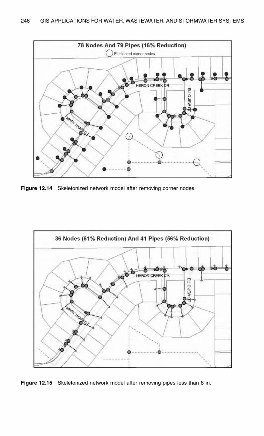
246 GIS APPLICATIONS FOR WATER, WASTEWATER, AND STORMWATER SYSTEMS
Figure 12.14 Skeletonized network model after removing corner nodes.
Figure 12.15 Skeletonized network model after removing pipes less than 8 in.

WATER MODELS 247
4. Small pipes with low flows can also be eliminated without significantly changingthe modeling results. There are no absolute criteria for determining which pipesshould be eliminated (Haestad et al., 2003). Elimination of pipes less than 6 in.or 8 in. is most common. Thus, small pipes and corresponding nodes can beeliminated for further network simplification. Figure 12.15 shows the skeletonizednetwork after removing pipes of less than 8 in. width. The most dramatic effect ofthis step is the removal of all the service lines from the network model. The networknow has 36 nodes and 41 pipes, representing a 56% reduction in the number oforiginal nodes and pipes. This moderate level of skeletonization is acceptable in mostcases.
5. Further reduction in the size of a network model is possible by aggregating thedemands from several customers to a single node. Figure 12.16 shows the skele-tonized network after dividing the network into three demand zones and assigningthe total zone demand to a node inside that zone. The network now has only 3nodes and 5 pipes, representing a 96% reduction in the number of original nodesand a 94% reduction in the number of original pipes. This high level of skeleton-ization can affect modeling results. For example, this model cannot model theflows and pressures at different houses within the subdivision.
Although the preceding steps can be performed manually in a GIS by editingthe data layers, the process will be too cumbersome unless the system is very small.Automatic GIS-based skeletonization that can be completed quickly is now avail-able in some software packages. Automatic skeletonization removes the complexityfrom the data, while maintaining the network integrity and hydraulic equivalencyof the system. Reductions of 10 to 50% in the size of a network are possible. Theseprograms allow the users to input the skeletonization criteria such as the smallest
Figure 12.16 Skeletonized network model after aggregating demand nodes.

248 GIS APPLICATIONS FOR WATER, WASTEWATER, AND STORMWATER SYSTEMS
Figure 12.17 Skeletonizer’s network simplification results. Top: original system with 2036pipes. Bottom: skeletonized network with 723 pipes (65% reduction). (Mapscourtesy of MWH Soft, Inc.)

WATER MODELS 249
pipe size that should be included in the model. The smallest-pipe-size criterionshould be used carefully because both size and accuracy of the skeletonized modeldepend on it. A highly skeletonized model does not work well in areas where mostof the water supply is through small pipes.
The Skeletonizer™ module of H2OMap water system modeling software(MWH Soft, Inc., Broomfield, Colorado, www.mwhsoft.com) and Skelebrator™
module of WaterCAD and WaterGEMS water system modeling software (HaestadMethods, Waterbury, Connecticut, www.haestad.com) are examples of softwaretools that automate the skeletonization of CAD and GIS layers. Figure 12.17 showsan example of Skeletonizer skeletonization. The top screenshot shows the originalnetwork with 2036 pipes imported from a GIS. The bottom screenshot shows theskeletonized network with 723 pipes, indicating a 65% reduction in the size ofthe network.
Mohawk Valley Water (MVW) is a water utility serving more than 125,000people in approximately 150 mi2 area in central New York. In 2002, MVW createdan all-pipe WaterCAD hydraulic model that was connected to a geodatabase. Areduce/skeletonize/trim (RST) process was used to eliminate hydrant laterals andprivate service connections to scale the hydraulic model to pipe segments 4-in. andgreater. The demands, pipe attributes, and elevations were extracted from the geo-database (DeGironimo and Schoenberg, 2002).
ESTIMATION OF NODE DEMANDS
Node demand is an important input parameter of a hydraulic model, representingthe water consumption rate in units of volume/time (e.g., gallons per day or liters persecond). Demands are grouped by customer type (e.g., residential, commercial, indus-trial, or institutional) or magnitude (e.g., average daily, maximum daily, peak hourly,or fire flow). Manual estimation of node demands from customer billing records is acumbersome process. Modelers, therefore, have traditionally resorted to approximatemethods, such as uniform distribution of the residential water use across all nodesfollowed by adding the nearest commercial and industrial use at various nodes. Thisapproach requires a significant effort in fine-tuning the node demands during themodel calibration phase of the project.
GIS allows implementation of more accurate demand estimation methods. Onesuch method utilizes the GIS to geocode (or geolocate) all individual water users(defined by the address at which each meter is located) and to assign the meteredwater consumption rates for each meter location to the nearest node in the model.The geocoding process links a street address to a geographic location and finds thecoordinates of a point location based on its street address. This method assumes thata computer file (spreadsheet or delimited text file) containing meter addresses andmetered water use for specified durations (e.g., quarterly or monthly) can be pro-duced from the utility’s billing database. If this information is available, the followingprocedure can be used to assign demands to nodes:

250 GIS APPLICATIONS FOR WATER, WASTEWATER, AND STORMWATER SYSTEMS
1. Create a GIS layer (e.g., a Shapefile) representing all nodes in the model.2. Obtain a street centerline layer of the system with address ranges. Such data can
also be purchased from commercial GIS data vendors (Shamsi, 2002).3. Obtain and preprocess customer meter location and consumption database.4. Process the meter address and street address range data in the GIS to geocode the
meter locations into a point layer registered to the model node layer.5. Process the geocoded meter data to assign and aggregate individual demands to
the nearest nodes.6. Analyze the assigned metered demand to determine unaccounted-for water and
metered demands that were not successfully geocoded. Uniformly distribute theseremaining demands across nodes.
7. Load the node demand data into the hydraulic model.
The preceding process produces a highly accurate distribution of water useacross the nodes. The intermediate product of point locations with associateddemands can also be used to visualize the spatial distribution of individual demandpoints throughout the system. A metered demand database can also be created toinclude customer classes as defined in the billing system. This data can be usedto assign differing demand patterns to residential, commercial, and industrialdemand classes for use in extended-period simulations.
Haestad Methods’ WaterGEMS hydraulic modeling software has a Loadbuildermodule that allows modelers to automatically calculate and assign demands tojunctions using the following three methods (Haestad Methods, 2002):
1. Customer meter data method: This method is used if geocoded customer billingdata are available. It assigns the demands to nodes using any combination of thefollowing three methods:• Nearest node method: This method assigns the meter demand to the nearest
node.• Nearest pipe method: This method assigns the meter demand to the two nodes
of the nearest pipe. Each node of the nearest pipe can receive equal demandsor weighted demands in proportion to its distance from the meter location.Alternatively, the demand can be assigned to the pipe node closest to the meterlocation.
• Meter aggregation method: This method creates service areas around thenodes of a hydraulic model. A service area polygon is associated with eachmodel node, enclosing all service connections that consume their water fromthe node and whose consumption is aggregated to that node. Service areascan be drawn manually or using automatic methods such as the TheissenPolygon method. Programs are available for automatic delineation of Theis-sen Polygons in a GIS package. All the meters located within a service areaare assigned to its associated node. Figure 12.18 shows the service areascreated using the Thiessen Polygon method in WaterGEMS software.
2. Area water use data method: This method is used if billing meter data are notavailable. It assigns the demands to nodes using the following three methods:• Equal flow distribution: This method requires a polygon layer for various
flow zones (e.g., meter routes or pressure zones) in the system. A GISoverlay of nodes and flow zone layers is conducted to divide each zone’sflow equally among all the nodes within that zone.

WATER MODELS 251
• Proportional distribution by area: In this method, a GIS overlay of service area(of nodes) and flow zone layers is conducted. Each zone’s flow is dividedamong all the service area polygons within that zone in proportion to the areaof service area polygons.
• Proportional distribution by population: In this method, a GIS overlay ofservice area (of nodes) and flow zone layers is conducted. Each zone’s flowis divided among all the service area polygons within that zone in proportionto the population of service area polygons. The service area population can becalculated in GIS by conducting an overlay of service area polygons withcensus-block* (or census-tract) polygons.
3. Land-use/population data method: This method forecasts the future demands fornodes using the following two methods:• Land-use data method: This method uses future land-use polygons to forecast
future demands. A GIS overlay of service area and land-use polygons isconducted to calculate the area of each land-use type within each service area.A demand factor (per unit area) is specified for each land-use type. Calculated
Figure 12.18 Example of meter aggregation method (WaterGEMS™ screenshot courtesy ofHaestad Methods).
* Census blocks and census tracts from U.S. Bureau of Census are polygon layers of demographic datafor the U.S. Additional information is available in Chapter 11.

252 GIS APPLICATIONS FOR WATER, WASTEWATER, AND STORMWATER SYSTEMS
land-use areas and demand factors are multiplied to estimate a future demandfor each service area.
• Population data method: This method uses projected future population poly-gons to forecast future demands. A GIS overlay of service area and populationpolygons is conducted to calculate the future population of each service area.A demand density (gallons per capita per day) is specified by the user. Calcu-lated future population and demand density are multiplied to estimate a futuredemand for each service area.
Detailed information on the preceding methods is available in Advanced WaterDistribution Modeling and Management (Haestad et al., 2003). For future land-usemapping techniques and information on how to calculate population from U.S.Bureau of Census GIS data (e.g., Census blocks and tracts), please refer to GIS Toolsfor Water, Wastewater, and Stormwater Systems (Shamsi, 2002).
Demand-Estimation Case Studies
Newport News, Virginia
In 1996, Newport News Waterworks (Newport News, Virginia) developed a watersystem hydraulic model composed of 540 nodes representing approximately 110,000service connections. The model contained all pipes 12 in. and larger and some 8 in.critical pipes. Model node demands were computed using the meter aggregationmethod described in the previous section. The service area polygons were drawnmanually, which was found to be the largest engineering effort required by themodeling project. A GIS Demand Application was developed to create, modify, ordelete model nodes and service area polygons. The application was developed usingArcTools, a collection of ArcInfo productivity tools implemented through an ArcMacro Language (AML) interface.
The demand data were extracted from a public utilities billing system.Average daily consumption of each customer was calculated by dividing thetotal consumption by the number of days in the billing cycle. The consumptiondata were loaded in a tabular GIS file. Account numbers were used to associatedemands with service connections. Consumption for all service connections thatgeographically fell within a service area polygon were aggregated. The aggre-gated consumption was stored as an attribute of the model node (Sevier andBasford, 1996).
Round Rock, Texas
The City of Round Rock (Texas) used Haestad Methods’ WaterCAD hydraulicmodeling software, ESRI’s ArcView GIS package, and Microsoft’s Access billingdatabase for estimating the node demands. Approximately 95% of the city’s 22,000water meters were assigned to precise geographic locations using geocoding. This

WATER MODELS 253
approach provided accurate node demand data and reduced model calibration time(Haestad Methods, 2002). The following steps were undertaken:
1. The geocoding process was performed in ArcView by linking the addresseswithin an existing parcels Shapefile to the billing address in the water meterdatabase.
2. Using WaterCAD’s Shapefile connection wizard, the node data from WaterCADwas synchronized to ArcView.
3. The modelers then drew polygons around the nodes and correspondingmeters.
4. ArcView was used to sum the demand data for the meters in each polygon.5. The total demand was applied to appropriate nodes.6. The junction file with the newly calculated node demands was synced back to
WaterCAD.
Lower Colorado River Authority, Texas
Pimpler and Zhan (2003) used an alternative grid-based (raster GIS) approachthat worked well for estimating water demand for Lower Colorado River Authority.The Authority serves more than 1 million customers in Texas in an area spanningmore than 29,800 mi2. Their method involved four steps:
1. Divide the service area into grid–cells.2. Calculate a score for each grid–cell based on weighted variables (e.g., land use,
proximity to employment centers, etc.) considered important for water demandanalysis.
3. Distribute the service area population proportionally to each grid–cell based onthe score assigned to each cell.
4. Estimate water demand associated with each cell based on its allocatedpopulation.
ESTIMATION OF NODE ELEVATIONS
Node elevation is also an important input parameter for a hydraulic model. It isusually defined by the ground elevation. Because 2.31 ft of elevation correspondsto 1 psi of water pressure, modeling water pressure to 1-psi precision requireselevation data accurate to approximately 2 ft. Table 12.4 provides the accuracy ofcommon sources of ground surface elevation. USGS topographic maps are generallyacceptable because an elevation accuracy of 5 ft is adequate for most nodes (Walski,2001).
Surveying provides the most accurate ground surface elevations. Unfortunately,surveying is very costly and time consuming and is recommended for critical modelnodes such as the centerline of a pump or a model calibration node (Walski, 2001).Manual estimation of node elevations from contour maps or as-built plans is also a

254 GIS APPLICATIONS FOR WATER, WASTEWATER, AND STORMWATER SYSTEMS
cumbersome process. A GIS allows automatic computation of node elevations fromDEM data using the following procedure:
1. Create a GIS layer (e.g., a Shapefile) for the nodes in the model.2. Obtain a DEM layer covering the water distribution service area.3. Georeference (georegister) the node and DEM layers (i.e., assign both layers the
same map projection system).4. Overlay the node layer over the DEM layer to assign DEM elevations to nodes.
Interpolate in between the DEM grid cells (pixels) to estimate the correct elevationat each node.
5. Load the node elevation data into the model.
Figure 12.19 shows an overlay of a water distribution system layer over a DEMlayer for calculating node elevations.
WaterGEMS has a TRex Wizard that automates extraction of elevation data froma DEM layer and assigns the extracted data to model nodes. TRex uses the precedingsteps to calculate node elevations. It interpolates in between the DEM pixels(grid–cells) rather than using a simple spatial join. A spatial join is less accurate
Table 12.4 Accuracy of Ground Elevation Data Sources
Source Accuracy (ft)
USGS 7.5-min 1:24,000-scale topographic maps 10USGS 30-m DEMs 5–10GPS survey — code phase 10GPS survey — carrier phase 1Digital orthophotos 1
Figure 12.19 Water distribution system draped over a DEM
WATER MODELS 255
because nodes that fall in between the DEM pixels would be assigned the elevationof the nearest cell.
PRESSURE ZONE TRACE
A GIS also allows identification of various pressure zones in a water distributionnetwork. This is done by selecting a network pipe or node that is part of a largerpressure zone. The GIS traces the water network in all possible directions until eithersources of water or assets (e.g., pressure regulating valves — PRVs) that isolatewater flow are found. All the pipes (or nodes) in the selected pressure zone arehighlighted. A buffer can be created around the highlighted features to create apolygon for the pressure zone boundary. Once the trace is complete, the user canassign a pressure zone attribute to the selected pipe or node.
CHAPTER SUMMARY
This chapter shows that GIS offers many useful applications for water distribu-tion systems. The applications described in this chapter indicate that GIS providesmany powerful and efficient tools for performing various hydraulic modeling taskssuch as network skeletonization, demand calculation and allocation, and elevationcalculations. The case studies and examples presented in the chapter illustrate thatmany water utilities are successfully using GIS applications for hydraulic modelingof their water distribution systems. Various software examples presented in thechapter indicate that many commercial off-the-shelf software packages are availableto help users benefit from hydraulic modeling applications of GIS.
CHAPTER QUESTIONS
1. Prepare a list of GIS applications for water distribution systems.2. Which hydraulic modeling tasks can be performed using GIS?3. What are the typical input parameters for a water distribution system hydraulic
model? Which of these parameters can be obtained from a GIS?4. List the GIS data layers that are useful for hydraulic modeling.5. How does a GIS help in presenting model output results?6. What is skeletonization? How does a GIS help this task?7. List the hydraulic models you are familiar with. Which of these models use a
GIS? Which method of GIS linkage (interchange, interface, or integration) dothey use?


257
CHAPTER 13
Sewer Models
GIS saves time and money in developing sewer system models forsimulating flows and depths in the collection system. GIS also helpsto prepare maps of the model results, which can be easily understoodby nonmodelers.
GIS-based sewer models bridge the gap between information and its recipients.

258 GIS APPLICATIONS FOR WATER, WASTEWATER, AND STORMWATER SYSTEMS
LEARNING OBJECTIVES
The learning objectives of this chapter is to understand how GIS can be appliedin developing sewer system hydraulic models, and to understand how GIS can beused to present modeling results
MAJOR TOPICS
• Representative sewer models• Storm Water Management Model (SWMM)• Graphical user interface (GUI)• SWMM applications• Data preparation• Interface development steps• GIS application case studies
LIST OF CHAPTER ACRONYMS
CMOM Capacity, Management, Operations, and MaintenanceCSO Combined Sewer OverflowDSS Decision Support SystemEPA (U.S.) Environmental Protection AgencyGUI Graphical User InterfaceHEC Hydrologic Engineering CenterHGL Hydraulic Gradient LineLTCP Long-Term Control Plan (for CSOs)NMC Nine Minimum Controls (for CSOs)NPDES National Pollution Discharge Elimination SystemODBC Open Database ConnectivityOLE Object Linking and EmbeddingSHC System Hydraulic Characterization (for CSOs)SSO Sanitary Sewer OverflowSWMM Storm Water Management Model
MAPINFO™ AND SWMM INTERCHANGE
In the late 1990s, Portland’s Bureau of Environmental Services (BES) developed asuite of GIS and database tools to develop data for SWMM models. Model data were
Application area Basement flooding modeling using the Interchange GIS Linkage Method described in Chapter 11 (Modeling Applications)
GIS software MapInfoModeling software SWMMOther software Microsoft Access GIS data Sewer pipes, aerial photographs, buildings and
parking lot polygonsGIS format Raster and vectorStudy area City of Portland, OregonOrganization Bureau of Environmental Services, City of Portland,
Oregon

SEWER MODELS 259
developed from maps and databases with automation of many of the steps for dataextraction, variable assignments, and model building. Detailed collection-system modelsof basins were developed to analyze local areas. These models contained essentially allof the pipes in the collection system and utilized two subcatchment definitions to placerunoff into the system in the correct location. Surface water subcatchments were definedas the areas that flowed into the sewer through street inlets in the public right-of-way.Direct connection subcatchments were defined as the areas that contributed to sanitaryand stormwater drainage through service laterals.
A GIS tool was developed to predict flooding of individual parcels by overlayingmodeled hydraulic gradient lines (HGLs) with estimated finished floor elevations obtainedfrom a DEM. Detailed SWMM RUNOFF and EXTRAN models were developed fromfacility maps and photogrammetric data with the use of a MapInfo GIS and a MicrosoftAccess database. The SWMM model showed that many of the system capacity problemswere in the local areas at the upstream ends of the system and that the local collection systemtended to hold water back from the downstream trunk sewers in the system. This betterunderstanding of where flooding was likely to occur and where system capacity constraintsactually occurred allowed BES a top-down view of the basin during alternatives analysis.Local inflow control alternatives were considered first, and pipe upsizing along with passingthe problem downstream was the second alternative. Figure 13.1 shows a thematic mapshowing flooding risk and historical complaints (Hoffman and Crawford, 2000).
GIS APPLICATIONS FOR SEWER SYSTEMS
GIS applications for sewer systems include (Shamsi, 2002):
• Performing H&H modeling of collection systems, including:• Automatic delineation of watersheds, sewersheds, and tributary drainage areas
Figure 13.1 Thematic map showing flooding risk and historical complaints (map courtesyof Computational Hydraulic Int.).

260 GIS APPLICATIONS FOR WATER, WASTEWATER, AND STORMWATER SYSTEMS
• Model simplification or skeletonization to reduce the number of manholes andsewers to be included in the H&H model
• Estimating surface elevation and slope from digital elevation model (DEM)data
• Estimating dry-weather sewage flow rates from land use, census data, and billingrecords
• Estimating wet-weather sewage flow rates from land use, soil, surface impervi-ousness, and slope
• Creating maps for wastewater National Pollution Discharge Elimination System(NPDES) permit requirements (as described in Chapter 9 [Mapping Applica-tions]), such as:• U.S. Environmental Protection Agency’s (EPA) combined sewer overflow
(CSO) regulations, such as System Hydraulic Characterization (SHC), NineMinimum Controls (NMC), and long-term control plan (LTCP)
• U.S. EPA’s sanitary sewer overflow (SSO) regulations, such as capacity, man-agement, operations, and maintenance (CMOM)
• Documenting field inspection data (as described in Chapter 15 [MaintenanceApplications]), including:• Work-order management by clicking on map features• Inspection and maintenance of overflow structures and manholes• Television (TV) inspection of sewers• Flow monitoring and sampling• Smoke-testing, dye-testing, and inflow/infiltration (I/I) investigations
• Performing and planning tasks such as assessment of the feasibility and impactof system expansion
In this chapter, we will focus on the sewer system H&H modeling applicationsof GIS.
SEWER SYSTEM MODELING INTEGRATION
Tight integration between a sewer model and a GIS is highly desirable.
The GIS applications in sewer system modeling are developed by using the threeapplication methods (interchange, interface, and integration) described in Chapter11 (Modeling Applications). These methods facilitate preparation of model-inputdata and mapping of model output results similar to their application for watersystem models described in Chapter 12 (Water Models).
Transfer of data between a GIS and a sewer model is handled differently bydifferent software vendors. Some products offer nothing more than a manual cut-and-paste approach for transferring data between a GIS and the model. Others offera truly integrated package. Obviously, tight integration between the sewer modeland the GIS is desirable. However, it should not be assumed that a tightly integratedmodel is the best modeling tool. For example, the interchange or interface capabilityof a comprehensive sewer model might be more useful for some users comparedwith a tightly integrated model having limited modeling capability to simulatecomplex situations such as surcharged sewers.

SEWER MODELS 261
SOFTWARE EXAMPLES
Sewer system modeling software is used to compute dry- and wet-weather flowfor hydraulic analysis and design of collection systems and wet-weather controlfacilities such as storage tanks and equalization basins.
Table 13.1 lists representative sewer system modeling packages and their GIScapabilities, vendors, and Web sites. The salient GIS features of some programs aredescribed in the following subsections.
What is common among the recent software developments is a transferabilityof fundamental database information, also referred to as a decision supportsystem (DSS). Under a DSS framework, neither the GIS nor the model is centralto the process. Both perform satellite functions for a central master database.(Heaney et al., 1999).
SWMM
Numerous hydrologic models were created in the U.S. during the 1970s,including the U.S. EPA’s legacy computer program SWMM and the U.S. ArmyCorps of Engineers’ Hydrologic Engineering Center’s HEC series of models(HEC-1 through 6). Two of the most popular models, HEC-1 and HEC-2, havebeen updated and renamed HEC-HMS and HEC-RAS.
Collection system hydraulics can be characterized by using an H&H computermodel such as SWMM. SWMM is a comprehensive computer model for analysisof quantity and quality problems associated with urban runoff. Both continuousand single-event simulation can be performed on catchments having sanitary
Table 13.1 Representative Sewer System Modeling Software
SoftwareGIS Linkage
Method Vendor Web Site
SWMM Interchange U.S. Environmental Protection Agency (EPA)
www.epa.gov/ceampubl/swater/swmm/index.htm
CEDRA AVSand Integration CEDRA Corporation www.cedra.com
H2OMAP Sewer H2OVIEW Sewer
Interface andIntegration
MWH Soft www.mwhsoft.com
InfoWorks CS and InfoNet
Interface and Integration
Wallingford Software
www.wallingfordsoftware.com
Mouse GM and MIKE SWMM
Interface DHI Water & Environment
www.dhisoftware.com
PCSWMM GIS Integration Computational Hydraulics Int.
www.computationalhydraulics.com
StormCAD and SewerCAD
Interface Haestad Methods www.haestad.com
XP-SWMM Interchange and Interface
XP-Software www.xpsoftware.com

262 GIS APPLICATIONS FOR WATER, WASTEWATER, AND STORMWATER SYSTEMS
sewers, storm sewers, or combined sewers and natural drainage, for prediction offlows, stages, and pollutant concentrations.
SWMM is one of the most successful models produced by EPA for the waste-water environment. SWMM was developed from 1969 to 1971 as a mainframecomputer program and has been continually maintained and updated. Versions 2,3, and 4 of SWMM were distributed in 1975, 1981, and 1988, respectively. Thefirst batch-mode microcomputer version of SWMM (Version 3.3) was released byEPA in 1983. The first conversational-mode user-friendly PC version of SWMM,known as PCSWMM, was commercially distributed in 1984 by ComputationalHydraulics, Inc., of Guelph, Ontario (Computational Hydraulics, 1995). The firstPC version of EPA’s SWMM was Version 4, which was distributed in 1988 (Huberand Dickinson, 1988; Roesner et al., 1988). An excellent review of SWMM’sdevelopment history can be found in the book by James (1993).
SWMM is regarded as the most widely used urban H&H model in the U.S.(Heaney et al., 1999). SWMM continues to be widely used throughout the worldfor analysis of quantity and quality problems related to stormwater runoff, combinedsewers, sanitary sewers, and other drainage systems in urban areas, with manyapplications in nonurban areas as well. From 1988 through 1999, the EPA Centerfor Exposure Assessment Modeling in Athens, Georgia, distributed approximately3600 copies of SWMM. The University of Florida distributed roughly 1000 copiesof SWMM in the late 1980s. Third-party interfaces for SWMM, such as MIKE-SWMM, PCSWMM, and XP-SWMM, have several thousand users. The numberof subscribers to the SWMM Users Group Internet discussion forum (Listserv) onthe Internet is nearly 10,000 (EPA, 2002).
The current version (4.3) was released by EPA in May 1994 for the 16-bitMS-DOS operating system. Professor Wayne Huber of Oregon State University,one of the authors of SWMM, has developed several updated versions of SWMM4. His latest version (4.4H) was updated in March 2002. All of these and previousSWMM versions were written in the FORTRAN programming language. Noneof them have a user interface or graphical capability. Users must provide ASCIItext input and rely on ASCII text output. EPA is currently developing an updatedversion of SWMM referred to as SWMM 5. Written in the C++ programminglanguage, SWMM 5 will incorporate modern software engineering methods aswell as updated computational techniques. The modular, object-oriented com-puter code of SWMM 5 is designed to simplify its maintenance and updatingas new and improved process submodels are developed. The new code will alsomake it easier for third parties to add GUIs and other enhancements to theSWMM engine. This approach follows the same approach used by the highlysuccessful EPANET model from EPA (described in Chapter 12 [Water Models]),which analyzes hydraulic and water quality behavior in drinking water distribu-tion systems (Rossman, 2000).
SWMM simulates dry- and wet-weather flows on the basis of land use, demo-graphic conditions, hydrologic conditions in the drainage areas, meteorologicalinputs, and conveyance/treatment characteristics of the sewer system. The modelercan simulate all aspects of the urban hydrologic and quality cycles, includingrainfall, snow melt, surface and subsurface runoff, flow routing through drainage

SEWER MODELS 263
network, storage, and treatment. Statistical analyses can be performed on long-term precipitation data and on output from continuous simulation. Figure 13.2shows a conceptual schematic of SWMM. This figure shows that SWMM is acomplex model capable of modeling various phases of the hydrologic cycle usingdifferent blocks (modules) such as RUNOFF, TRANSPORT, and EXTRAN.
SWMM can be used both for planning and design. Planning mode is usedfor an overall assessment of the urban runoff problem or proposed abatementoptions. SWMM is commonly used to perform detailed analyses of conveyancesystem performance under a wide range of dry- and wet-weather flow conditions.These days, SWMM is frequently used in the U.S. for modeling wet-weatheroverflows including CSO, SSO, and stormwater discharges from collection sys-tems. As such, it is the model of choice for use in many collection-systemmodeling studies. For example, SWMM can be used to develop a CSO modelto accomplish various tasks leading to the development of a CSO Plan of Actionsmandated by EPA. These tasks include characterizing overflow events, develop-ing the CSO vs. rainfall correlation, maximizing the collection-system storage,and maximizing the flow to the treatment plant. The CSO model can also beused to develop the EPA-mandated LTCPs to evaluate various CSO controloptions. Sizing of CSO control facilities such as a wet-weather equalization tankrequires CSO volume and peak discharge, both of which can be modeled usingSWMM.
The use of SWMM to model wet-weather overflows is particularly advantageousfor the following reasons:
• SWMM produces estimates of present and future dry- and wet-weather flowrates. Flow estimates can be prepared based upon present and future land-use
Figure 13.2 SWMM conceptual schematic.

264 GIS APPLICATIONS FOR WATER, WASTEWATER, AND STORMWATER SYSTEMS
conditions, topography, sewer characteristics, and selected meteorological con-ditions. The model can be calibrated against measured flow rates.
• SWMM models the performance of the conveyance system under a range ofdynamic flow conditions.
• Using SWMM, it is possible to assess hydraulic capacity in response to wet-weather input. This characteristic can be very useful for analyses related toabatement of overflows.
SWMM is flexible enough to allow for different modeling approaches to thesame area. An approach that adequately describes the service area and accuratelycomputes and routes the flows at reasonable computing time and effort should beadopted. The following modeling strategy is generally used for modeling wet-weather overflows:
• Delineate sewersheds (the drainage areas tributary to overflows, also referred toas subareas or subbasins).
• Use the TRANSPORT Block to generate sewershed dry-weather flows.• Use the RUNOFF Block to generate sewershed wet-weather flows.• Combine dry-weather and wet-weather flows to generate combined sewershed
flows.• Use the EXTRAN Block to route the flows through the collection and interceptor
system.
USEFUL SWMM WEB SITES
SWMM Graphical User Interface
Most users have now become accustomed to modeling in a point-and-clickcomputing environment that provides a user-friendly graphical user interface(GUI). A GUI is a computer program that acts as an interpreter between usersand their computers. It is designed to minimize (but not eliminate) the need forhuman experts and to guide the modeler through the intricacies of a particularnumerical model. A GUI provides a suite of tools to create a decision supportsystem for the numerical model that has been adopted. It also stimulates userinterest and facilitates interpretation of model results. A GUI improves produc-tivity by increasing the efficiency of data entry, eliminating data errors throughexpert-checking, and the use of decision-support graphics and interpretation tools.It replaces difficult-to-remember text commands by interactive computer graphicsconsisting of menus, dialogue boxes, input and output windows, and icons. Themain goal of using GUIs is to develop user-friendly computer applications or to
SWMM4 www.epa.gov/ceampubl/swater/swmm/index.htmSWMM5 www.epa.gov/ednnrmrl/swmm/Oregon State University ccee.oregonstate.edu/swmm/SWMM-Users Internet Discussion Forum
www.computationalhydraulics.com/Community/Listservers/swmm-users.html
SWMM-Online www.swmm-online.com

SEWER MODELS 265
add user-friendliness to existing command-line-driven applications. For example,Microsoft Internet Explorer is a GUI for user-friendly access to the Internet.
Modern software offer pull-down menus, toolbars, icons, buttons, dialogueboxes, hypertext, context-sensitive online help, etc., which are not available in legacycomputer programs including SWMM 4. Many commercial modeling packages nowoffer on-screen point-and-click drawing and editing of drainage network maps, butunfortunately some legacy programs still rely on ASCII text input and output files.SWMM was developed in an era when input files were created on punched cards.After 30 years, SWMM 4 now runs on personal computers, but it is still a text-based,nongraphical DOS program. It reads ASCII input to produce ASCII output, which ismost suitable for mainframe line printers. SWMM’s ASCII format output is long,boring, difficult to interpret, and not very useful for nonmodelers. Creating computermodels and reviewing the model results is often slowed by our inability to see thesystem being modeled. It is up to the modeler to review SWMM’s voluminous outputand construct a mental image of the physical system being modeled. Often, thelimitation in understanding the model output has been the modeler’s own comprehen-sion of the output, not the model itself. Quite frequently, it is impossible for the modelerto absorb the large amount of information contained in the model output (TenBroekand Roesner, 1993).
A GUI and a GIS can be employed to overcome SWMM’s input/output defi-ciencies. Two types of GUIs can be employed for GIS applications in SWMMmodeling (Shamsi, 1997; Shamsi, 1998):
• An input interface (also called a front-end interface or preprocessor) extractsSWMM input from GIS layers and creates SWMM’s traditional ASCII text inputfile. The input GUIs can also provide graphical tools to draw a network modelthat is subsequently converted to SWMM’s ASCII input file. For example, aninput interface may extract sewer-segment lengths and manhole coordinates fromthe sewer and manhole layers.
• An output interface (also called a back-end interface or postprocessor) convertstext to graphics. It can convert SWMM’s traditional ASCII text output file tographs, charts, plots, and thematic maps that can be easily understood byeveryone.
With the help of these GUI/GIS tools, everybody can understand the modeloutput. These tools help one to see storm-surge progress through the sewer systemand pinpoint areas of flooding and surcharging. More than just reams of computerpaper, such models become automated system-evaluation tools. Other benefits ofGUI/GIS tools are:
• Preparation of network schematics is not essential. Digitized plots of sewers andsubarea boundaries can be used to create a drainage network diagram on a com-puter screen.
• Zoom and pan features make it possible to display even the largest networksconveniently on the screen.
• Connectivity data errors are easily detected and can be edited while still in theprogram. Instabilities in the model output, often the most difficult errors to find,are also easily located.

266 GIS APPLICATIONS FOR WATER, WASTEWATER, AND STORMWATER SYSTEMS
• Flow and depth data from SWMM output can be displayed in either plan or profileview, providing an animated display of the HGL during the simulation time steps.
• Flow and HGL time-series plots can be displayed for any conduit or node in thehydraulic network.
• Field-collected flow and depth data can be displayed along with the model outputfor model calibration and verification.
• Network graphics and modeled hydrographs can be exported to word processorsto aid in report preparation.
XP-SWMM and XP-GIS
XP-SWMM by XP Software (Belconnen, Australia and Portland, Oregon) isa full-fledged 32-bit Microsoft Windows application. The program has beenenhanced by the addition of a graphics database, and an adaptive dynamic wavesolution algorithm that is more stable than the matrix method used in the originalSWMM. The program is divided into a stormwater layer, which includes hydrologyand water quality; a wastewater layer, which includes storage treatment and waterquality routing for BMP analysis; and a hydrodynamic/hydraulics layer for sim-ulation of open or closed conduits (Heaney et al., 1999).
XP-SWMM is also included in Visual SWMM from CaiCE Software Corp.(Tampa, Florida). Basically, XP-SWMM and Visual SWMM are GUI programsfor SWMM. The user-friendly GUI is based upon a graphical representation of
Figure 13.3 Visual SWMM screenshot.

SEWER MODELS 267
the modeled system using a link-node architecture. It provides a shell that acts asan interpreter between the user and the model. It facilitates on-screen developmentof a SWMM model in the form of a link-node network. Figure 13.3 shows a VisualSWMM (Version 7) screenshot.
Because the links and nodes are set up on a coordinate-system basis, files canbe translated between most CAD and GIS software systems using the interchangemethod. CAD or GIS files can also be used as a backdrop for the system beingmodeled. Although XP-SWMM is not linked or integrated to a GIS package, itprovides an optional utility called XP-GIS to extract model input data from theexisting GIS database tables. XP-GIS is a module for linking XP-SWMM to GISdatabases. Its main purpose is to facilitate the import and export of modeling datafrom GIS and other data sources such as spreadsheets, asset management software,and OLE/ODBC compliant databases. It also allows for the inclusion of Shapefilesas background layers and for data to be viewed and manipulated in an XP-SWMMgraphical environment.
GIS Data for SWMM
GIS layers for land use, elevation, slope, soils, and demographics can be pro-cessed to extract model parameters for input to various SWMM Blocks and othercollection system models. The basic input parameters to be assembled into theRUNOFF Block input files include sewershed area, overland flow slope, overlandflow width, percent imperviousness, roughness coefficients, and soil infiltrationparameters. Area, slope, and percent imperviousness can be computed from the GISlayers. Table 13.2 shows sample sewershed RUNOFF data extracted from GIS layersusing the interchange method for a study area in Pennsylvania.
GIS layers can also be used to estimate inputs for sewershed population, pop-ulation density, number of houses, average family size, average market value ofhouses, average family income, and the predominant land-use type for the TRANS-PORT Block. Table 13.3 shows sample sewershed TRANSPORT data extractedfrom GIS layers using the interchange method for a study area in Pennsylvania.
Estimating Green-Ampt Parameters Using STATSGO/SSURGO GIS Files
Based on their resolution, there are three types of U.S. Natural Resources Con-servation Service (NRCS) (formerly the U.S. Soil Conservation Service or SCS)soils data that are useful in GIS applications:
• National Soil Geographic (NATSGO)• State Soil Geographic (STATSGO)• Soil Survey Geographic (SSURGO)
SSURGO provides the highest resolution soils data at scales ranging from1:12,000 to 1:63,360. This resolution is appropriate for watersheds a few squaresmiles in area. STATSGO data are digitized at 1:250,000-scale, which is useful when

GIS
AP
PLIC
AT
ION
S F
OR
WA
TE
R, W
AS
TE
WA
TE
R, A
ND
ST
OR
MW
AT
ER
SY
ST
EM
S268
Table 13.2 Sample GIS Data for SWMM’s RUNOFF Block
Sewershed Area
(Acres)Mean
PI Mean
% Slope
Land Use (Acres)
S.F.R. M.F.R. Comm. Ind. O.S. S.W.
2 397.82 25.46 7.78 168.79 — — 45.90 183.12 — 4 20.18 44.30 5.81 14.81 — 0.47 4.65 0.24 — 5 4.13 35.00 4.34 — — 4.13 — — — 6 31.58 43.90 6.87 25.24 1.79 4.54 — — — 7 116.82 16.60 11.70 41.42 1.90 — — 73.51 — 8 29.66 76.50 4.52 — 10.14 18.89 — 0.63 — 9 38.95 38.73 4.50 35.43 1.54 1.98 — — —10 13.93 40.50 6.39 11.55 2.06 0.31 — — —11 16.69 31.30 6.86 13.46 0.24 0.25 — 2.74 —12 29.47 27.60 9.13 22.18 — — — 7.29 —13 13.86 21.60 9.76 7.68 — — — 6.18 —14 18.49 26.20 7.56 13.07 — — — 5.42 —15 64.49 17.40 13.63 26.64 — — — 37.85 —16 84.24 23.19 8.49 46.04 2.52 — — 35.68 —17 29.13 50.40 9.15 5.10 — — 17.47 6.56 —18 84.93 21.50 7.10 46.67 — — — 38.26 —19 31.76 33.20 7.12 22.84 0.01 — 3.13 5.77 —20 159.91 38.41 6.47 118.24 10.71 4.57 11.75 14.63 —21 58.43 52.10 5.87 30.98 12.92 5.79 8.75 — —23 78.67 39.20 6.72 36.66 — — 23.78 18.23 —24 77.83 33.00 6.79 72.52 — 0.01 — 5.31 —25 297.06 22.60 5.52 166.87 3.77 — — 126.41 0.0226 5.05 35.00 18.55 5.05 — — — — —27 45.16 33.30 6.94 28.96 1.56 — 4.70 9.95 —28 21.82 45.70 5.70 13.84 — — 7.05 0.93 —29 28.79 49.50 5.11 16.90 3.10 0.02 8.75 — 0.0130 9.71 61.10 3.47 3.07 3.92 2.68 — 0.04 —32 33.46 46.90 4.64 24.47 2.47 6.51 — — —35 24.97 41.90 5.24 18.84 — 4.41 — 1.70 0.04 37 8.82 40.20 6.70 7.60 — — 1.23 — —38 30.77 54.20 4.93 14.83 7.78 4.35 3.80 — —
S21 13.43 25.33 8.88 9.10 — — — 4.33 —Total/Mean 1920.01 37.24 7.26 1068.85 66.43 58.91 140.96 584.78 0.07
Notes: P.I. = Percent Imperviousness; S.F.R. = Single-Family Residential; M.F.R. = Multifamily Residential; Comm. = Commercial; Ind. = Industrial;O.S. = Open Space; and S.W. = Surface Water.

SEWER MODELS 269
analyzing large regional watersheds. NATSGO data describe variations in soil typeat the multistate to regional scale, which is not suitable for wastewater and storm-water modeling applications (Moglen, 2000).
The steps for estimating Green-Ampt parameters using STATSGO GIS data aregiven in the following text:
1. Download the STATSGO database files from the NRCS Web site (www.ftw.nrcs.usda.gov/stat_data.html).• comp.dbf — Attribute HYDGRP has Hydrologic Soil Groups (A, B, C, etc.)• layer.dbf — Attribute TEXTURE2 has soil texture (S [sand], SIL [silt], etc.)
2. Join the soils layer to the preceding tables using the MUID attribute that providesa common link between the soils layer and the STATSGO database files.
Table 13.3 Sample GIS Data for SWMM’s TRANSPORT Block
Sewershed PopulationPopulation
DensityFamily
SizeFamilyIncome
MarketValueHouses
2 944 2.37 406 2.3 27,709 58,491 4 165 8.18 73 2.3 19,777 36,823 5 15 3.63 13 1.2 19,777 34,180 6 359 11.37 177 2.0 20,461 39,054 7 363 3.11 150 2.4 27,708 50,258 8 223 7.52 156 1.4 17,227 42,920 9 504 12.94 242 2.1 22,184 46,114 10 195 14.00 102 1.9 16,375 38,077 11 191 11.44 88 2.2 16,639 37,734 12 241 8.18 106 2.3 19,540 35,694 13 38 2.74 17 2.2 21,439 33,337 14 98 5.30 43 2.3 21,439 38,712 15 282 4.37 132 2.1 23,260 52,256 16 330 3.92 148 2.2 21,439 48,634 17 47 1.61 20 2.3 21,439 56,297 18 717 8.44 321 2.2 19,192 36,142 19 501 15.77 234 2.1 16,610 33,060 20 2,282 14.27 1,127 2.0 19,769 36,348 21 774 13.25 437 1.8 19,237 31,908 23 659 8.38 282 2.3 17,454 33,436 24 761 9.78 374 2.0 22,598 29,289 25 1,301 4.38 576 2.3 22,642 46,708 26 23 4.55 11 2.0 22,646 26,955 27 403 8.92 178 2.3 16,480 31,922 28 260 11.92 119 2.2 16,889 29,544 29 410 14.24 186 2.2 16,214 26,441 30 94 9.68 56 1.7 14,814 28,387 32 247 7.38 110 2.2 12,783 33,810 35 102 4.08 48 2.1 13,074 38,263 37 26 2.95 10 2.6 21,439 56,620 38 421 13.68 220 1.9 18,369 39,140
Total/Mean 12,976 8.14 6,162 2.10 19,568 38,921

270 GIS APPLICATIONS FOR WATER, WASTEWATER, AND STORMWATER SYSTEMS
3. Perform an overlay of soils with subareas layer to estimate:• Percentage of HYDGRP in each subarea• Percentage of TEXTURE2 in each subarea
4. Calculate the Green-Ampt parameters (saturated hydraulic conductivity KS, initialmoisture deficit IMD, and average capillary suction SU) for each subarea usingthe look-up tables shown in Table 13.4. These look-up tables are based on thedata provided in SWMM’s users manual (Huber and Dickinson, 1988).
GIS APPLICATIONS FOR SWMM
Representative GIS applications in SWMM modeling are given in the followingsubsections.
AVSWMM
Shamsi (1997) developed an ArcView GIS interface called AVSWMM forcollection-system and wet-weather overflow modeling. Both RUNOFF and EXT-RAN Blocks were included. The interface was developed by customizing ArcView3.2, using Avenue. Avenue is ArcView’s native scripting language and is built intoArcView 3.x. Avenue’s full integration with ArcView benefits the user in two ways:(1) by eliminating the need to learn a new interface and (2) by letting the user work
Table 13.4 Sample EXTRAN Input Data
KS Look-Up Table
HYDGRP KS
A 0.375B 0.225C 0.100D 0.025
MD Look-Up Table
Soil TEXTURE2 KS
Sand S 0.31Sandy loam SL 0.28Silt loam IL 0.26Loam L 0.23Sandy clay loam SCL 0.18Clay loam CL 0.16Clay C 0.13
SU Look-Up Table
Soil TEXTURE2 SU
Sand S 4Sandy loam SL 8Silt loam SIL 12Loam L 8Clay loam CL 10Clay C 7

SEWER MODELS 271
with Avenue without exiting ArcView (ESRI Educational Services, 1995). Figure13.4 shows ArcView’s integrated programming interface, using Avenue.
The AVSWMM interface was developed as two separate extensions, one eachfor the RUNOFF and the EXTRAN Blocks of SWMM.
AVSWMM RUNOFF Extension
When the extension is loaded, a menu named SWMM is added to the ArcViewinterface as shown in Figure 13.5. The SWMM menu has seven calculators andtwo functions that calculate various RUNOFF Block parameters for subareas (sew-ersheds). A polygon layer for subareas is required to use this extension. ArcView’sSpatial Analyst Extension is required for the analysis of raster data layers. Eachcalculator prompts the user for the layer containing the subareas and the layercontaining the data from which the model parameter is to be extracted. Eachcalculator adds the calculated input parameters to fields in the subarea layer. Thefields are created if they do not exist. Various functions and calculators of thisextension are described in the following text:
1. Average Slope Calculator
Function Assigns average slope to subareas Input Layers Subarea polygon layer
Slope grid Output Adds or updates MEANSLOPE field in subarea layer
2. Census Parameter Calculator
Function Assigns total population and housing counts to subareas
Figure 13.4 ArcView 3.x integrated programming interface for writing avenue scripts.

272 GIS APPLICATIONS FOR WATER, WASTEWATER, AND STORMWATER SYSTEMS
Input Layers Census block polygon layerSubarea polygon layer
Output Adds or updates total population and housing fields to subareasPop100 Total PopulationHu100 Total HouseholdsPopDens Population density per acreHouseDens Households density per acreMnFamSize Mean family size
3. Land Use Calculator
Function Calculates area of each land use class for subareas Input Layers Landuse grid layer
Subarea polygon layer Output Adds fields for each land use type to subarea layer
Calculates area for each land use type
Figure 13.5 AVSWMM RUNOFF Extension.

SEWER MODELS 273
4. Percent Imperviousness Calculator
Function Assigns percentage of percent imperviousness for each subarea.The calculator will add a percent impervious field to the landusepolygon layer and will prompt for the percent impervious valuefor each land use type.
Input Layers Landuse grid layerSubarea polygon layer
Output Adds or updates field containing percent impervious, PERIMP, to subarea layer
5. Set Soil Look-up Tables Function
Function Joins the look-up tables for soil infiltration parameters for theGreen-Ampt method (Huber and Dickinson, 1988)IMD Initial moisture deficitKS Saturated hydraulic conductivity or permeabilitySU Capillary suctionAdditional information is presented below
Input Layers Soils polygon layerIMD.dbf look-up tableKS look-up tableSU look-up table
Output Joins the look-up tables to the soils layer
6. Soil Parameter Calculator
Function Calculates Green-Ampt infiltration parameters, IMD, KS, and SUfor subareas. The user may also select any numerical fields of theSoils layer to average.
InputLayers Soil polygon layerSubarea polygon layer
Output Adds or updates average soil parameters to subarea layer MNIMD Mean IMD valueMNKS Mean KS valueMNSU Mean SU value
7. Manhole Elevation Calculator
Function Assigns elevation to manholes based from a DEMInput Layers DEM grid
Manhole point layerOutput Adds or updates ELEV field containing elevation to Manhole layer
8. Make Curve Number Grid Function
Function Prepares a grid layer for runoff curve numbersInput Layers Land use layer
Soil polygon layerSubarea polygon layer
Output It overlays the land use and soil layers to make a curve numbergrid. The values of the grid are based on each unique combinationof land use and hydrologic soil group.
9. Curve Number Calculator
Function Calculates subarea runoff curve numbers. Although EPA’s SWMMrelease does not use runoff curve numbers for input, many hydro-logic models (e.g., HEC-HMS) and some SWMM GUI programs,such as XP-SWMM (described above) can use this parameter.

274 GIS APPLICATIONS FOR WATER, WASTEWATER, AND STORMWATER SYSTEMS
Input Layers Curve number gridSubarea polygon layer
Output Calculates the average curve number for each subarea. The valuesare added to the CURVNUM field of the Subarea layer.
AVSWMM EXTRAN Extension
Development of the AVSWMM EXTRAN Extension required the two main tasksdescribed below:
Task 1: Create EXTRAN input file
This task requires that ArcView-compatible GIS layers (themes) exist withattribute fields for all model input parameters. The interface fetches the model inputparameters from the GIS layers and exports (copies) them to an ASCII text inputfile specified by the user. The user should create a header file containing the modelcontrol parameters. The control parameters are entered on the A1 line (title) andon B0 to B9 lines (solution and printing instructions). The interface automaticallyappends this header file to the input file. A simplified example is given in thefollowing text:Given Data:
1. ArcView GIS layer for manholesManholes layer attributes:
• ID• Bottom elevation• Top elevation• Inflow rate
2. ArcView GIS layer for sewersSewers layer attributes:
• ID• Upstream manhole• Downstream manhole• Type (circular, rectangular, etc.)• Depth (diameter for circular pipes)• Width (not required for circular pipes)• Length• Material• Date installed (material and date installed can be used to automatically
calculate Manning’s roughness coefficient)• Upstream invert elevation• Downstream invert elevation
Data To Be Created: An ASCII text input file containing the following parameters:
• Junction (usually manhole) data:• Data type (D1 for junctions)• Manhole number• Top elevation (GR-EL)

SEWER MODELS 275
• Bottom elevation (INV-EL)• Inflow rate• Initial depth (Y0, usually 0.0)
• Conduit (usually sewer pipe) data:• Data type (C1 for conduits)• Pipe number• Upstream junction (FR)• Downstream junction (TO)• Initial flow (Q0, usually 0.0)• Type (1 for circular, 2 for rectangular, etc.)• Area (0.0 for circular and rectangular)• Depth (DEEP = diameter for Type 1, depth for Type 2)• Width (WIDE = width for Type 2)• Length (LEN)• ZP1 (upstream invert elevation minus upstream node bottom elevation)• ZP2 (downstream invert elevation minus downstream node bottom
elevation)• N (Manning’s roughness coefficient, a function of pipe material and age)• STHETA and SPHI (usually zero, required for open channels only)
Note that ZP1, ZP2, and N are not part of the given sewer’s data, but can beestimated in ArcView from the given data. For example, if the material is concreteand the age of the pipe is less than 10 years (fair condition), then ArcView can usea look-up table to estimate N as 0.015. ZP1 and ZP2 can be similarly estimatedfrom the upstream and downstream manhole data. Sample SWMM input lines forjunctions and conduits are shown in Table 13.5.
Table 13.5 Sample EXTRAN Input Data
Sample EXTRAN Input Data Lines for Junctions
* JUNCTION DATA* ID GR-EL INV-EL INFLOW Y0D1 10 554.7 522.0 0.0 0.0D1 20 551.1 522.3 0.0 0.0D1 30 554.7 522.7 0.0 0.0D1 40 553.5 523.0 0.0 0.0D1 50 550.6 524.6 0.0 0.0
Sample EXTRAN Input Data Lines for Conduits
* CONDUIT DATA* ID FR TO Q(0) TYPE AREA DEEP WIDE LEN ZP1 ZP2 N STHETA SPHIC1 330 50 40 0.0 1 0.0 6.0 0.0 820 0.0 0.0 0.015 0.0 0.0C1 331 40 30 0.0 1 0.0 6.0 0.0 173 0.0 0.0 0.015 0.0 0.0C1 332 30 20 0.0 1 0.0 6.0 0.0 200 0.0 0.0 0.015 0.0 0.0C1 333 20 10 0.0 1 0.0 6.0 0.0 140 0.0 0.0 0.015 0.0 0.0

GIS
AP
PLIC
AT
ION
S F
OR
WA
TE
R, W
AS
TE
WA
TE
R, A
ND
ST
OR
MW
AT
ER
SY
ST
EM
S276
Table 13.6 Sample EXTRAN Output Data
Sample EXTRAN Output Data for Junctions
Junction Summary Statistics
Junction Number
GroundElevation
(FT)
UppermostPipe
Crown Elevation
(FT)
MeanJunctionElevation
(FT)
Junction Average
% Change
MaximumJunctionElev. (FT)
Time of OccurenceHr. Min.
Feet ofSurcharge
At Max Elevation
Feet Max.Depth is Below
GroundElevation
Length ofSurcharge
(Min)
Length ofFlooding
(Min)
Maximum Junction
Area(FT2)
10 554.70 528.00 527.74 3.1377 554.59 8 30 26.59 0.11 69.5 0.0 8.717120 551.10 528.30 528.14 2.2338 551.10 8 30 22.80 0.00 60.8 0.5 9.878130 554.70 528.70 528.69 1.9667 551.55 8 30 22.85 3.15 60.8 0.0 1.084140 553.50 529.00 529.03 1.7722 551.40 8 30 22.40 2.10 60.7 0.0 2.8831
50 550.60 530.60 530.72 1.2461 548.47 8 30 17.87 2.13 60.3 0.0 5.3431
Sample EXTRAN Output Data for Conduits
Conduit Summary Statistics
ConduitNumber
DesignFlow(CFS)
DesignVelocity
(FPS)
ConduitVerticalDepth
(IN)
MaximumComputed
Flow(CFS)
Time ofOccurence
MaximumComputed
Velocity(FPS)
Time ofOccurence
Ratio ofMax. toDesignFlow
MaximumInv. at
Upstream(FT)
Depth AboveConduit EndsDownstream
(FT)
Lengthof Norm
Flow(Min)
ConduitSlope
(FT/FT)Hr. Min. Hr. Min.
330 1.62E+02 5.73 72.00 2.10E+02 9 4 7.43 9 4 1.30 23.87 28.40 46.3 0.00195331 1.53E+02 5.41 72.00 2.11E+02 9 2 7.45 9 2 1.38 28.40 28.85 22.2 0.00173332 1.64E+02 5.81 72.00 3.21E+02 8 35 11.35 8 35 1.96 28.85 28.80 4.8 0.00200333 1.76E+02 6.22 72.00 3.52E+02 8 35 12.45 8 35 2.00 28.80 32.46 10.3 0.00214

SEWER MODELS 277
Task 2: Create SWMM EXTRAN output layers in ArcView GIS
This task creates model output layers in ArcView by reading EXTRAN’s ASCIItext output file. A database table of the relevant output results is created from theoutput file. The output database file is then temporarily joined to ArcView layers(usually the pipes layer). The linked output results can then be queried or used toclassify a legend. A simplified example is given in the following text:Given Data: EXTRAN’s ASCII text output file. Sample SWMM output lines forjunctions and conduits are shown in Table 13.6.Data to Be Created
• An ArcView layer for manhole SWMM output• An ArcView layer for pipe SWMM output
As shown in Figure 13.6, the AVSWMM EXTRAN interface adds a SWMMmenu to ArcView’s main menu. This menu has four functions: Make Input File,Read Output, Join Results, and Unjoin Results. The interface allows a user tocreate an EXTRAN input file, translate an output result file, join the output resultfile to the themes, and remove the results joined to the themes. All model runsthat have been translated are eligible to be viewed. Model run data are stored inseparate folders. AVSWMM EXTRAN functions are described in the followingtext.Make Input File: This menu choice creates an EXTRAN input file. As shown inFigure 13.7, the user is prompted for a model input name. The input file is placedin a folder called name, which is under the project directory. If the folder does notexist, it is created. The function prompts for a description of the model run. It is astring that is inserted in the input file as a comment line. The function then promptsfor an optional header file to attach to the input file. The header files have an extensionof .hdr and are created separately by the user in a text editor. The header file containsEXTRAN input file data other than C1 and D1 records, which are already stored inthe “name.inp” file.Read Output: This menu choice translates an EXTRAN output file into GIS databasefiles. The function prompts for an output file to translate. The program assumes theuser has run the SWMM model from the input file created previously. The outputfile should be located in the same folder as the input file. The program translatesthe Conduit Summary and Junction Summary Statistics tables of the EXTRANoutput into GIS databases named condsum.dbf and junctsum.dbf and stores them inthe “name” folder. The function also writes a file “name.res” in the project directory.The .res file contains the absolute path to the directory where the model results arestored. This file indicates that a model has been translated. It is used to find allmodel runs available for linking.Result Join: This menu choice temporarily joins the translated EXTRAN output tothe ArcView attribute tables of manholes and sewers. The tool prompts the user toselect a model run to link. The routine temporarily links the result databases to theattribute data. The result data can now be queried, listed, or used to classify a legend.Figure 13.8 shows ArcView database tables showing imported EXTRAN results.

278 GIS APPLICATIONS FOR WATER, WASTEWATER, AND STORMWATER SYSTEMS
Figure 13.9 shows a thematic map of maximum sewer flows based on classifyingthe Q(MAX) output variable from the EXTRAN output.Unjoin Results: This menu choice reverses (unjoins) the link between the SWMMoutput and the ArcView attribute tables established by the “Results Join” menuchoice. The purpose of this menu choice is to undo the last import of SWMM outputto ArcView if the user does not like the SWMM results and wants to rerun SWMMand import the output again.
SWMMTools
SWMMTools is an ArcView extension developed by Heineman (2000). Inspiredby Shamsi’s work described in the preceding subsections, it allows users of SWMM4.4 to visualize a SWMM model in conjunction with existing GIS data. SWM-MTools links SWMM input and output files with ArcView GIS. It allows viewingof model input and output summary data within ArcView. The extension adds a
Figure 13.6 AVSWMM EXTRAN Interface.
Figure 13.7 AVSWMM EXTRAN: Make Input File feature.

SEWER MODELS 279
Figure 13.8 EXTRAN results in ArcView.
Figure 13.9 Thematic map of maximum sewer flows.

280 GIS APPLICATIONS FOR WATER, WASTEWATER, AND STORMWATER SYSTEMS
single pull-down menu to ArcView. Three scripts load plan views of RUNOFF,TRANSPORT, or EXTRAN conduit networks. Three scripts link SWMM outputwith existing RUNOFF, TRANSPORT, and EXTRAN GIS themes respectively. Twoscripts work with a stormwater catchment theme to facilitate catchment parameter-ization. One estimates RUNOFF catchment widths. Another estimates RUNOFFimpervious area fractions (parameter DCIA) from GIS land-use data.
AGSWMM
Existing SWMM4-ArcView3 interfaces such as AVSWMM and SWMMToolsdescribed in the preceding subsections will continue to work with SWMM4 andArcView3 Unfortunately, these interfaces cannot work with SWMM5 or ArcView/ArcGIS8 and higher versions because of the following reasons:
1. SWMM4 and SWMM5 input file formats are different2. SWMM4 and SWMM5 output file formats are different3. SWMM4 and SWMM5 have different data structures (e.g., three different
representations of the same pipe are not required in Runoff, Transport, andExtran Blocks)
4. ArcView3 interfaces are written in Avenue, which is not compatible withArcView8
To benefit from new features of the new software versions, new interfaces shouldbe developed. Shamsi and Smith (2004) developed a SWMM5-ArcView8 interfacecalled ArcGIS SWMM (AGSWMM). The main features of AGSWMM are listedbelow:
• AGSWMM links SWMM5 with ArcGIS• AGSWMM was developed using VBA• AGSWMM setup installs a DLL file• AGSWMM adds a new “ArcSWMM” toolbar in ArcGIS• AGSWMM allows creation of a SWMM5 input file from GIS layers• AGSWMM allows creation of a SWMM5 backdrop map (.emf file) in ArcGIS• AGSWMM allows on-screen editing of input parameters in ArcGIS• AGSWMM allows thematic mapping of SWMM5 output in ArcGIS
Figure 13.10 shows the AGSWMM toolbar. The toolbar consists of two tools:SWMM Input and SWMM Results View. The SWMM Input tool opens the inputform shown in Figure 13.10. It allows users to create the SWMM5 input file. Theleft side of the form is used for creating input data for nodes (e.g., manholes).The right side of the form is used for creating input data for links (or conduits,e.g., pipes). Users can assign the appropriate GIS layer attributes to SWMM5input parameters using dropdown pick lists. Users can either create a newSWMM5 input file using the “Make SWMM Input File” button at the bottom ofthe input form, or they can update the input parameters in an existing SWMM5input file by selecting the “Synchronize SWMM File” button. The synchronization
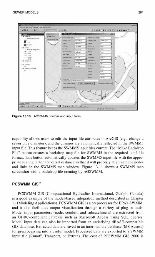
SEWER MODELS 281
capability allows users to edit the input file attributes in ArcGIS (e.g., change asewer pipe diameter), and the changes are automatically reflected in the SWMM5input file. This feature keeps the SWMM5 input files current. The “Make BackdropFile” button creates a backdrop map file for SWMM5 in the required .emf fileformat. This button automatically updates the SWMM5 input file with the appro-priate scaling factor and offset distance so that it will properly align with the nodesand links in the SWMM5 map window. Figure 13.11 shows a SWMM5 mapscreenshot with a backdrop file creating by AGSWMM.
PCSWMM GIS™
PCSWMM GIS (Computational Hydraulics International, Guelph, Canada)is a good example of the model-based integration method described in Chapter11 (Modeling Applications). PCSWMM GIS is a preprocessor for EPA’s SWMM,and it also facilitates output visualization through a variety of plug-in tools.Model input parameters (node, conduit, and subcatchment) are extracted froman ODBC-compliant database such as Microsoft Access using SQL queries.Model input data can also be imported from an underlying dBASE-compatibleGIS database. Extracted data are saved in an intermediate database (MS Access)for preprocessing into a useful model. Processed data are exported to a SWMMinput file (Runoff, Transport, or Extran). The cost of PCSWMM GIS 2000 is
Figure 13.10 AGSWMM toolbar and input form.

282 GIS APPLICATIONS FOR WATER, WASTEWATER, AND STORMWATER SYSTEMS
$400. Figure 13.12 shows the PCSWMM GIS interface that has been developedusing Visual Basic and resembles the ArcView GIS interface.
SWMM and BASINS
EPA has shown an interest in incorporating SWMM into its BASINS package,which is already integrated with the ArcView GIS software. EPA is now developinga SWMM linkage to its BASINS package. This link would be a valuable tool forurban planners and watershed managers to evaluate the urban pollution load inrelation to other loads in the watershed and provide a more holistic view ofwatershed management. This project is being done through an EPA Office ofAdministration and Resources Management (OARM) contract with Lockheed
Figure 13.11 SWMM5 map window with a backdrop file created in ArcGIS.

SEWER MODELS 283
Martin Information Services (LMIS). When completed, this project will bundleSWMM and BASINS together with HSPF, TOXIROUTE, and QUAL2E programsthat are currently part of the BASINS modeling environment. It should also allowextraction of SWMM input data from the GIS files that are part of the BASINSCD-ROMs. Detailed BASINS information is presented in Chapter 11 (ModelingApplications).
SWMMDUET
The Delaware Department of Natural Resources and Environmental Control,Division of Soil and Water, developed this program in 1994. SWMMDUET isan example of SWMM and GIS integration. This program integrates SWMM4.2 (1993) with ArcInfo (ARC/INFO) 6.0. For this reason, it does not functionwith the latest versions of SWMM and ArcInfo (Schell et al., 1996). It has beenwritten in ArcInfo’s native Arc Macro Language (AML). It creates a computingenvironment that does not require arcane knowledge of SWMM and ArcInfo.SWMMDUET incorporates a preprocessor and a postprocessor, and therefore,provides interfaces both for creating SWMM’s input file and for graphingSWMM’s output file. SWMMDUET takes advantage of the graphical paradigmaround which ArcInfo was constructed and utilizes relational database capabil-ities to organize data. Beyond data management, the program uses expert-system
Figure 13.12 PCSWMM GIS: an example of a model-based integration method.
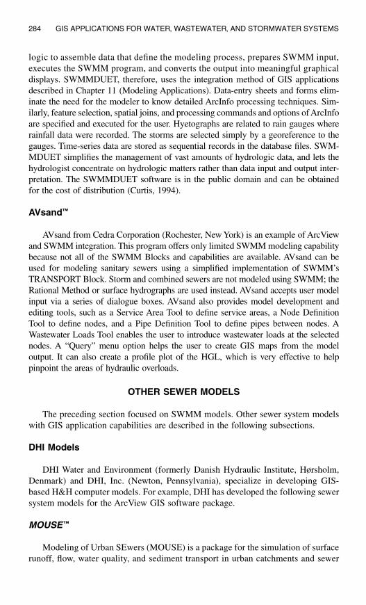
284 GIS APPLICATIONS FOR WATER, WASTEWATER, AND STORMWATER SYSTEMS
logic to assemble data that define the modeling process, prepares SWMM input,executes the SWMM program, and converts the output into meaningful graphicaldisplays. SWMMDUET, therefore, uses the integration method of GIS applicationsdescribed in Chapter 11 (Modeling Applications). Data-entry sheets and forms elim-inate the need for the modeler to know detailed ArcInfo processing techniques. Sim-ilarly, feature selection, spatial joins, and processing commands and options of ArcInfoare specified and executed for the user. Hyetographs are related to rain gauges whererainfall data were recorded. The storms are selected simply by a georeference to thegauges. Time-series data are stored as sequential records in the database files. SWM-MDUET simplifies the management of vast amounts of hydrologic data, and lets thehydrologist concentrate on hydrologic matters rather than data input and output inter-pretation. The SWMMDUET software is in the public domain and can be obtainedfor the cost of distribution (Curtis, 1994).
AVsand™
AVsand from Cedra Corporation (Rochester, New York) is an example of ArcViewand SWMM integration. This program offers only limited SWMM modeling capabilitybecause not all of the SWMM Blocks and capabilities are available. AVsand can beused for modeling sanitary sewers using a simplified implementation of SWMM’sTRANSPORT Block. Storm and combined sewers are not modeled using SWMM; theRational Method or surface hydrographs are used instead. AVsand accepts user modelinput via a series of dialogue boxes. AVsand also provides model development andediting tools, such as a Service Area Tool to define service areas, a Node DefinitionTool to define nodes, and a Pipe Definition Tool to define pipes between nodes. AWastewater Loads Tool enables the user to introduce wastewater loads at the selectednodes. A “Query” menu option helps the user to create GIS maps from the modeloutput. It can also create a profile plot of the HGL, which is very effective to helppinpoint the areas of hydraulic overloads.
OTHER SEWER MODELS
The preceding section focused on SWMM models. Other sewer system modelswith GIS application capabilities are described in the following subsections.
DHI Models
DHI Water and Environment (formerly Danish Hydraulic Institute, Hørsholm,Denmark) and DHI, Inc. (Newton, Pennsylvania), specialize in developing GIS-based H&H computer models. For example, DHI has developed the following sewersystem models for the ArcView GIS software package.
MOUSE™
Modeling of Urban SEwers (MOUSE) is a package for the simulation of surfacerunoff, flow, water quality, and sediment transport in urban catchments and sewer

SEWER MODELS 285
systems. MOUSE combines complex hydrology, hydraulics, water quality model-ing, and sediment transport modeling capabilities in a graphical and easy-to-useinterface. MOUSE is a 32-bit Windows application specifically designed to operatewithin Microsoft Windows and Windows NT operating systems, and is optimizedfor fast simulations and graphics. Both metric (SI) and imperial units are supported.The MOUSE system is organized in several modules:
• MOUSE Runoff: Surface-runoff models for urban catchment applications• MOUSE HD: Hydrodynamic network model with some limited RTC capabilities• MOUSE RDII: Advanced hydrological model for continuous simulation• MOUSE RTC: Advanced reactive RTC capabilities for MOUSE pipe models• MOUSE LTS: Long-term hydraulic simulations with statistics• MOUSE SRQ: Pollutant buildup and transport on catchments surfaces• MOUSE AD: Pollutant advection-dispersion in drainage networks• MOUSE WQ: Water quality processes in drainage networks• MOUSE ST: Sediment transport in drainage networks
Some of these modules are marketed as optional add-on modules to the standardconfiguration. The various modules together with the user interface part, includingthe time-series and cross-section editors, advanced graphics both on the input andoutput sides, and the online HELP system, make the MOUSE system a desirablesewer system modeling package. MOUSE is a sophisticated hydraulic model thatis commonly compared to SWMM (Heaney, 1999).
MIKE SWMM ™
MIKE SWMM is DHI’s implementation of SWMM. Resulting from a collabo-rative effort between DHI and Camp, Dresser, and McKee (CDM), MIKE SWMMcombines the power of SWMM with a user-friendly interface. Data can be digitizedand viewed with background images and edited with the same graphical editors thatare also part of the MOUSE system. Data can also be entered and edited throughdatabase forms, which include scrollable spreadsheet-like sections for efficient edit-ing of tabulated data. These different editors or views of the same information aredynamically linked, so that changes introduced through one editor are automaticallyand instantly updated in the other views. MIKE SWMM’s database tool for storageof network data gives access to a range of query options.
MOUSE GIS™
MOUSE GIS is an application linking the MOUSE numerical sewer modelingsystem with ArcView. MOUSE GIS is an interface between ArcView and theMOUSE model. The MOUSE GIS interface is used for preprocessing externaldatabase information into MOUSE data sets. Once the link to an external databaseis established, manhole, link, weir, pump, and catchment data can be uploaded.The entire database can be used for the model networks, or a subset can be

286 GIS APPLICATIONS FOR WATER, WASTEWATER, AND STORMWATER SYSTEMS
selected. The selected set can subsequently be simplified (nodes excluded) toreduce the model size. MOUSE GIS also acts as a postprocessor for simulationresults. Pipe flow results (maximum flow, velocity, depth and surcharge, flooding,etc.) can be displayed and overlayed with other GIS data. Mouse GIS alsoprovides an interface to MIKE SWMM. Figure 13.13 shows a MOUSE GISscreenshot of the sewer system model for the city of Ljubljana (Slovenia) devel-oped by DHI. The figure also shows the results of network skeletonizationperformed by MOUSE GIS. The automatic skeletonization has reduced the net-work size to 40%.
MOUSE GM ™
MOUSE GM (in which MOUSE GIS is embedded), an ArcView-based modulefor MIKE SWMM and MOUSE users, promotes spatial and visual representationof the model and provides a direct link to GIS databases. MOUSE GM includesmodel-simplification tools that enable the user to create simplified (skeletonized)models from detailed data sets. This productivity tool may save days or weeks oftedious and error-prone work in the early phases of modeling projects. MOUSE GMreads and writes the SWMM file formats. It can be used as the ArcView GIS linkand model-simplification tool for all SWMM modeling packages that apply the
Figure 13.13 MOUSE GIS screenshot showing network skeletonization results.

SEWER MODELS 287
standard SWMM data formats. With MOUSE GM, MIKE SWMM users can linkto GIS databases and with any asset management system that supports ODBCconnectivity.
InfoWorks™
Wallingford Software Ltd. (Wallingford, U.K.) develops and supplies data man-agement, operation, and simulation software for the water industry worldwide. Itoffers two main software products for sewer system modeling:
• InfoWorks CS (formerly HydroWorks): Integrates asset and business planningwith urban drainage network modeling.
• InfoNet: Provides tools, reports, displays, and data management capabilities. Itintegrates with GIS, desktop office systems, hydraulic modeling systems, main-tenance management systems (MMS), field data systems, SCADA, and corporatedatabases. Data exchange interfaces have been designed not only for import andexport purposes but also to connect directly with GIS (ArcView and MapInfo),hydraulic modeling systems (InfoWorks), SCADA, and logger systems. InfoNethas been designed to ensure that data exchange with Microsoft Windows appli-cations and geographic information systems is a seamless operation.
InfoWorks CS is recognized for its fast, efficient, and stable algorithms forwastewater modeling. It models systems containing complex pipe connections,complex ancillary structures and static or variable control devices, open channelsand trunk sewers, full backwater effects, and reverse flow. It can be upgraded toinclude one or more of the following optional modules:
• Water Quality module: Predicts quality components, volume of spillage andfloods, and helps develop cost-effective solutions to pollution and sedimentationproblems.
• Real Time Control (RTC) module: Allows central management of flow throughoutan entire network and local flow control at individual ancillary structures. RTChelps users maximize wastewater system storage, optimize flow routing, optimizeoperation of ancillary structures, and design cost-effective systems.
InfoWorks products are designed to link H&H models with GIS and infor-mation management systems. InfoWorks CS combines a relational database withspatial analysis. It can be used to transfer data to and from third-party applications.One can also import asset data directly from Microsoft Access or .CSV files intothe InfoWorks database. For instance, InfoWorks CS allows importing of sub-catchment areas, area breakdown, and population data directly from MapInfoProfessional, ArcView, or GeoMedia Professional GIS. Figure 13.14 shows theInfoWorks CS output results imported in MapInfo Professional (top) and ArcView(bottom).
In Figure 13.14, nodes are symbolized according to modeled flood volume in cubicmeters, which represents the water overflowing from a manhole. Smaller (green) nodesare OK (no overflow), those in light blue and slightly larger are loosing a small amount

288 GIS APPLICATIONS FOR WATER, WASTEWATER, AND STORMWATER SYSTEMS
of water, those in dark blue and larger are loosing lots of water. Link theme is showingsurcharge depth. This represents 0.1 to 0.5 of pipe height (up to half full), 0.5 to 0.99of pipe height (between half full and completely full), 1.0 of pipe height, or 100%full, and then 2.0, which is pressurized flow. The associated colors are black, lightblue, dark blue and purple.
Figure 13.14 InfoWorks CS results in MapInfo Professional (top) and ArcView 3.2 (bottom).
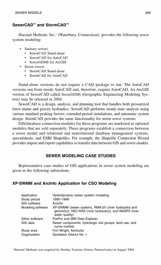
SEWER MODELS 289
SewerCAD™ and StormCAD™
Haestad Methods, Inc.* (Waterbury, Connecticut), provides the following sewersystem modeling:
• Sanitary sewers• SewerCAD Stand-alone• SewerCAD for AutoCAD• SewerGEMS for ArcGIS
• Storm sewers• StormCAD Stand-alone• StormCAD for AutoCAD
Stand-alone versions do not require a CAD package to run. The AutoCADversions run from inside AutoCAD and, therefore, require AutoCAD. An ArcGISversion of SewerCAD called SewerGEMS (Geographic Engineering Modeling Sys-tem) may be released in 2004.
SewerCAD is a design, analysis, and planning tool that handles both pressurizedforce mains and gravity hydraulics. SewerCAD performs steady-state analysis usingvarious standard peaking factors, extended-period simulations, and automatic systemdesign. StormCAD provides the same functionality for storm sewer systems.
GIS/database connection modules for these programs are marketed as optionalmodules that are sold separately. These programs establish a connection betweena sewer model and relational and nonrelational database management systems,spreadsheets, and ESRI Shapefiles. For example, the Shapefile Connection Wizardprovides import and export capabilities to transfer data between GIS and sewer models.
SEWER MODELING CASE STUDIES
Representative case studies of GIS applications in sewer system modeling aregiven in the following subsections.
XP-SWMM and ArcInfo Application for CSO Modeling
* Haestad Methods was acquired by Bentley Systems (Exton, Pennsylvania) in August 2004.
Application Hydrodynamic sewer system modelingStudy period 1995–1998GIS software ArcInfoModeling software XP-SWMM (sewer system), RMA-2V (river hydraulics and
geometry), HEC-RAS (river hydraulics), and WASP5 (river water quality)
Other software FoxPro and IBM Data ExplorerGIS data Sewer components, hydrologic soil groups, land use, and
curve numberStudy area Fort Wright, KentuckyOrganization Sanitation District No. 1

290 GIS APPLICATIONS FOR WATER, WASTEWATER, AND STORMWATER SYSTEMS
The Sanitation District No. 1 (the District) located in northern Kentucky used GIS,GPS, RDBMS, and computer modeling technologies to simulate virtual flows of sewagethrough pipes, CSOs, and into and through local rivers (Ohio and Licking Rivers). Withthe concurrent tasks of updating the GIS and starting up of the facility plan, a commondatabase was developed. The objective of the database was to provide a central locationwhere data could be stored and used for the benefit of both tasks. An XP-SWMMManagement System (XMS) was developed within FoxPro, which acts as the translatorbetween different software packages. By including all five data sources (roads andstreams, rain-gauge data, XP-SWMM output, CSO loadings, and fecal coliformresponse of receiving water), a more complete cause–effect relationship was developed.The visualization of the system using IBM Data Explorer provided an overall pictureof the system that was not available before. This case study is a good example of GISbeing used as an integrator technology or integrating platform (Martin et al., 1998).
AM/FM/GIS and SWMM Integration
MWRA serves the sewerage needs of over two million people in 43 commu-nities in the Boston metropolitan area. It was estimated that nearly half the flowin their system is a direct result of rainfall-induced inflow and infiltration (I/I)due to deteriorated sewers and manholes. In order to evaluate both the short-termand long-term needs of their sanitary sewer interceptor system, MWRA initiatedand completed a sewage analysis and management system (SAMS) project, whichinvolved linking of ArcInfo, CASS WORKS, and SWMM using the interfacemethod of model integration. ArcInfo was used to create a link between SWMMdata and computerized maps of the MWRA interceptor system and communitiesserved. The maps were used as both a tool to input different planning scenariosinto the CASS WORKS system and as a visual medium to geographically showthe model results. The integrated AM/FM/GIS system was installed on a multiuserDEC VAX 4000-200. The integrated model allowed the MWRA planners topredict the I/I reduction from elimination of groundwater and rainwater from theinterceptor system. Elimination of these flows resulted in significant operationalcost savings to the MWRA and its ratepayers (ESRI, 1994).
SWMM and ArcInfo™ Interface
This application was developed as part of a watershed approach to assessing theecological health of Bayou Chico, which is a subestuary of Pensacola Bay. BayouChico is the receiving water body of small, mostly urbanized watersheds located in
Application Sewer system modeling using the interface methodGIS software ArcInfoModeling software SWMMOther software CASS WORKS (RJN Environmental Associates)Study area Boston, Massachusetts, metropolitan areaOrganization Massachusetts Water Resources Authority (MWRA)

SEWER MODELS 291
southern Escambia County, Florida. A GIS database and the use of remotely sensedsatellite images were combined to determine surface characteristics, storm drainagesystems, area, and slope of the watershed. These data layers were in turn linked toSWMM, which mathematically represents these physical characteristics and uses thisinformation to determine both runoff and pollutant loading. The SWMM RUNOFFBlock was broken into a hydrological component and a pollutant loading component.Both have parameters that may be retrieved from spatially based data. Pollutant loadingis partially determined either by land-use class or gutter length. Gutter length can bederived from digitized road layers or are available for some metropolitan areas in theU.S. Census TIGER data files. ArcInfo tools allowed for querying of polygons forareal extent, perimeter, length, width, and other associated attributes. AML program-ming was used to query ArcInfo layers for SWMM parameter data and to write theinformation to an ASCII text file in the SWMM input file format (Schell et al., 1996).
Hydra™ and ArcInfo™ Interface
The City of Stockton, California, developed an interface between their ArcInfoGIS and Pizer’s HYDRA/HydraGraphics sewer and stormwater modeling software.The GIS contained sanitary sewers and land-use layers, and was utilized as the rawdata source for developing a sewer model for master planning purposes. To facilitatethis process, a customized GIS data management interface was developed usingArcView GIS as the graphical interface between the City’s GIS and the sewer model.This interface included several project-specific Avenue routines to import the City’sGIS layers, extract the system model and land-use data, and export the modelcomponents to the sewer model (Prins et al., 1998).
USEFUL WEB SITES
CHAPTER SUMMARY
This chapter shows that GIS offers many useful applications in sewer system H&Hmodeling. GIS applications are developed using the three methods of interchange,interface, and integration as described in Chapter 11 (Modeling Applications). Theinterface method seems to be the most prevalent method at the present time. The casestudies and examples presented in the chapter illustrate that many sewer utilities aresuccessfully using GIS applications for modeling their sewer systems. The software
Danish Hydraulic Institute www.dhisoftware.comHaestad Methods www.haestad.comMWH Soft www.mwhsoft.comSWMM www.epa.gov/ceampubl/swater/swmm/index.hm
www.epa.gov/ednnrmrl/swmm/SWMM-Online www.swmm-online.comWallingford Software www.wallingfordsoftware.com

292 GIS APPLICATIONS FOR WATER, WASTEWATER, AND STORMWATER SYSTEMS
examples presented in the chapter indicate that many public-domain (e.g., SWMM)and commercial-off-the-shelf software packages (e.g., MOUSE) are available to helpusers benefit from sewer system modeling applications of GIS.
CHAPTER QUESTIONS
1. Prepare a list of GIS applications for sewer systems.2. What is a GUI? How does it help modelers?3. Which sewer system modeling tasks can be performed using GIS?4. What are the typical input parameters for a sewer system hydraulic model? Which
of these parameters can be obtained from a GIS?5. List the GIS data layers that are useful for sewer system modeling.6. How does GIS help in presenting the output results of a sewer system model?7. List the sewer system models you are familiar with. Which of these models use
GIS? Which method of GIS linkage (interchange, interface, or integration) dothey use?
8. Is a GIS-integrated sewer model always better than a stand-alone model? Providereasons for your answer.

293
CHAPTER 14
AM/FM/GIS Applications
At present our water and wastewater infrastructure, especially in theolder cities, is in critical stages of deterioration and has started tocrumble. AM/FM/GIS technology provides a spatial infrastructuremanagement approach that is very effective in prioritizing yourinfrastructure improvement and maintenance needs.
Field inspection crews inspecting a combined sewer overflow (CSO) diversion chamber locatednear Pittsburgh, Pennsylvania.

294 GIS APPLICATIONS FOR WATER, WASTEWATER, AND STORMWATER SYSTEMS
LEARNING OBJECTIVE
The learning objective of this chapter is to find out how GIS is integrated withautomated mapping/facilities management (AM/FM) systems for efficient inspectionand maintenance of water industry infrastructure.
MAJOR TOPICS
• Infrastructure maintenance issues• AM/FM/GIS basics• AM/FM/GIS software• AM/FM/GIS application examples
LIST OF CHAPTER ACRONYMS
AM/FM/GIS Automated Mapping/Facilities Management/Geographic InformationSystem
CAD Computer-Aided Drafting/Computer-Aided Design CAFM Computer-Aided Facility ManagementCCTV Closed-Circuit TelevisionCIFM Computer Integrated Facility ManagementCMMS Computerized Maintenance Management System GASB Government Accounting Standards Board RBE Rule Base EngineRDBMS Relational Database Management SystemsSDE Spatial Database Engine
HAMPTON’S WASTEWATER MAINTENANCE MANAGEMENT
Hampton, Virginia, has a population of 150,000 and has 12,000 manholes andvalves. The City conducted a GPS survey to collect coordinates of more than 8000manholes located in alleys, buried in yards, or covered with asphalt. The City utilizesmore than 35 licenses of ArcView GIS. The City stored attribute data in an externalinfrastructure database from GBA Master Series and linked it to ArcView GIS. TheGBA software performs infrastructure inventory of manholes and pipes, work-ordermanagement, and parts inventory management. It can also interface with the City’sWinCan system used for CCTV inspection of sewers. The GBA GIS Toolkit, an
GIS software ArcView, GBA GIS Toolkit Extension for ArcView, MapObjectsInternet Map Server (IMS)
Other software GBA Master Series and WinCan TV systemGIS data Sewers, manholes, water mains, valves, hydrants, roads,
street centerlines, buildings, and digital orthophotos Study area City of Hampton, VirginiaProject duration 1998–2001Organization Public Works Department, Hampton, Virginia
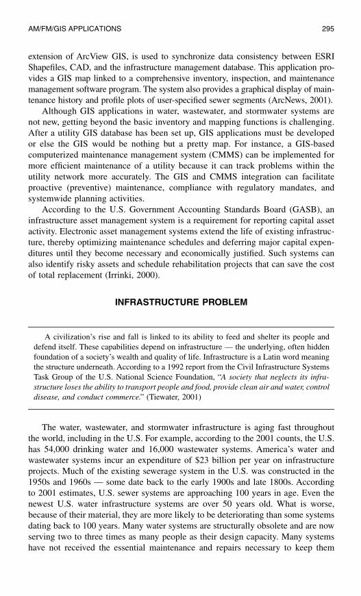
AM/FM/GIS APPLICATIONS 295
extension of ArcView GIS, is used to synchronize data consistency between ESRIShapefiles, CAD, and the infrastructure management database. This application pro-vides a GIS map linked to a comprehensive inventory, inspection, and maintenancemanagement software program. The system also provides a graphical display of main-tenance history and profile plots of user-specified sewer segments (ArcNews, 2001).
Although GIS applications in water, wastewater, and stormwater systems arenot new, getting beyond the basic inventory and mapping functions is challenging.After a utility GIS database has been set up, GIS applications must be developedor else the GIS would be nothing but a pretty map. For instance, a GIS-basedcomputerized maintenance management system (CMMS) can be implemented formore efficient maintenance of a utility because it can track problems within theutility network more accurately. The GIS and CMMS integration can facilitateproactive (preventive) maintenance, compliance with regulatory mandates, andsystemwide planning activities.
According to the U.S. Government Accounting Standards Board (GASB), aninfrastructure asset management system is a requirement for reporting capital assetactivity. Electronic asset management systems extend the life of existing infrastruc-ture, thereby optimizing maintenance schedules and deferring major capital expen-ditures until they become necessary and economically justified. Such systems canalso identify risky assets and schedule rehabilitation projects that can save the costof total replacement (Irrinki, 2000).
INFRASTRUCTURE PROBLEM
A civilization’s rise and fall is linked to its ability to feed and shelter its people anddefend itself. These capabilities depend on infrastructure — the underlying, often hiddenfoundation of a society’s wealth and quality of life. Infrastructure is a Latin word meaningthe structure underneath. According to a 1992 report from the Civil Infrastructure SystemsTask Group of the U.S. National Science Foundation, “A society that neglects its infra-structure loses the ability to transport people and food, provide clean air and water, controldisease, and conduct commerce.” (Tiewater, 2001)
The water, wastewater, and stormwater infrastructure is aging fast throughoutthe world, including in the U.S. For example, according to the 2001 counts, the U.S.has 54,000 drinking water and 16,000 wastewater systems. America’s water andwastewater systems incur an expenditure of $23 billion per year on infrastructureprojects. Much of the existing sewerage system in the U.S. was constructed in the1950s and 1960s — some date back to the early 1900s and late 1800s. Accordingto 2001 estimates, U.S. sewer systems are approaching 100 years in age. Even thenewest U.S. water infrastructure systems are over 50 years old. What is worse,because of their material, they are more likely to be deteriorating than some systemsdating back to 100 years. Many water systems are structurally obsolete and are nowserving two to three times as many people as their design capacity. Many systemshave not received the essential maintenance and repairs necessary to keep them

296 GIS APPLICATIONS FOR WATER, WASTEWATER, AND STORMWATER SYSTEMS
working properly. The American Society of Civil Engineers (ASCE) projects $1.3trillion in infrastructure needs in the U.S. during 1999 to 2004, of which approxi-mately one third is needed for water and wastewater improvements.
Unfortunately, adequate government funds are not available for this expensivefix. This problem can be partially blamed on the “out-of-sight, out-of-mind” men-tality of the decision makers. The lack of funding for the badly needed infrastructureimprovements is making people worried. This is evident in the recently conductedpublic opinion polls. According to a recent Water Environment Federation (WEF)survey, 31% of Americans would not swim in their own rivers. A 1998 ASCE pollshowed that more than 75% of the U.S. voters were concerned about the quality ofroads, drinking water, and school buildings. In Boston, more voters were concernedabout roads, bridges, and drinking water than Social Security and taxes. In NewYork City, concerns about school buildings and drinking water outscored drug abuseworries (ASCE, 1998). Many indicated that they would vote for a candidate whoseelection campaign addressed waste disposal (78%), drinking water (73%), and roadsand bridges (62%). These surveys indicate that water industry infrastructure isparticularly important because it is so closely related to public health and safety.
In the U.S., it has been recently observed that a combination of reduced federalspending and increased federal mandates is taking its toll on the infrastructure ofthe country. For instance, according to American Water Works Association (AWWA),annual pipe replacement costs will jump to $3 billion by 2020 and $6 billion by2030. Replacement expenses projected into the future indicate that sewer mainreplacements are more urgent than water mains and will require more money.
As of 2001, ASCE estimates that the U.S. must invest nearly $277 billion indrinking water and wastewater infrastructure repairs over the next two decades. U.S.water systems have an $11-billion annual investment shortfall and need $151 billionby 2018. U.S. sewer systems have a $12-billion annual shortfall in investment andneed $126 billion by 2016. The largest need, $45 billion, is for projects to controlcombined sewer overflows (CSOs). The second-largest category of needs, at $27billion, is for new or improved secondary treatment.
In a report “Water Infrastructure Now” published in February 2001, a waterconservation organization called Water Infrastructure Network (WIN) estimated a$23-billion per year gap between infrastructure needs and current spending. Thereport indicated that U.S. water and wastewater systems faced infrastructure fundingneeds of nearly $1 trillion over the next 20 years and a shortfall of half a trilliondollars. The report called for a 5-year, $57-billion federal investment in waterinfrastructure to replace aging pipes and upgrade treatment systems. WIN estimatesthat household water bills must double or triple in most U.S. communities if utilitiesare forced to absorb the entire infrastructure bill. For instance, the City of Gloucester,Massachusetts, is charging $20,000 per home (to be paid over the next 20 years) tofinance the city’s conversion from septic to sewer systems (CE News, 2001).
According to a 2001 statement by ASCE President Robert W. Bein, “Something isterribly wrong … America has been seriously underinvesting in its infrastructure.”

AM/FM/GIS APPLICATIONS 297
In March 2001, ASCE released its 2001 Report Card (Figure 14.1) for America’sinfrastructure in which the nation’s infrastructure received a cumulative grade of D+for 12 infrastructure areas. Causes for such a dismal grade include: explosive pop-ulation growth and school enrollment, which outpace the rate and impact of currentinvestment and maintenance efforts; local political opposition and red tape, whichoutpace the development of effective solutions; and the growing obsolescence of anaging system — evident in the breakdown of California’s electrical generationsystem and the nation’s decaying water infrastructure. The 2001 Report Card followsthe one released in 1998, at which time the ten infrastructure categories rated weregiven an average grade of D. The 2001 wastewater grade declined from a D+ to a D,while drinking water remained a D. Solid waste and schools scored the highest andthe lowest grades, respectively (ASCE, 2001; EWRI, 2001). Despite the disturbingfindings contained in the 2001 Report Card, the nation failed to heed the call toimprove its deteriorating infrastructure, according to an update to the assessmentreleased by ASCE in September 2003 (ASCE, 2003).
When the infrastructure condition is bad and funding is scarce, we need infra-structure management tools that can:
• Accurately define (or map) our infrastructure• Identify the worst portions of the infrastructure• Determine how to most cost-effectively improve (replace or repair) the worst parts
of the infrastructure
AM/FM/GIS products provide an efficient infrastructure management system.
AM/FM/GIS BASICS
Many solutions for managing facilities have spawned from CAD-based archi-tectural applications. Database solutions have evolved from the financial sector to
Figure 14.1 ASCE Infrastructure Report Card for the U.S.

298 GIS APPLICATIONS FOR WATER, WASTEWATER, AND STORMWATER SYSTEMS
include scheduling, inventory, and purchasing functions. Implementation of facilitymanagement automation can occur at any scale, from a small spreadsheet recordingpreventative maintenance items to a full corporate system with CAD capabilitiesmanaging the complete maintenance process with integrated contracting, accounting,inventory, asset, and personnel records. CAD-based products have normally beenclassified as computer-aided facility management (CAFM), whereas the databasesolutions, dealing with work-order management without a CAD component, havebeen termed computerized maintenance management systems (CMMS). The FMuser community reflects this polarization, because the majority of current imple-mentations are oriented either one way or the other. Computer integrated facilitymanagement (CIFM) brings both CMMS and CAFM capabilities into synergy,thereby addressing the implementation of a true facility management automationprogram. The core consideration is that, in practice, CMMS and CAFM capabilitiesaugment and are essential to each other. For example, maintenance activities keepthe data required for planning accurate and up-to-date (GEOTELEC, 2004).
AM/FM/GIS is a combination of four separate systems:
• Automated Mapping (AM)• Facilities Management (FM)• Automated Mapping/Facilities Management (AM/FM)• Geographic Information System (GIS)
The differences between the three systems are summarized in Table 14.1 andillustrated in Figure 14.2.
Automated Mapping (AM)
Automated mapping (AM), also known as computer-aided mapping (CAM), isa CAD application for producing maps. It can be considered an alternative to thetraditional manual cartographic maps. Data are organized in layers that are concep-tually like registered film overlays. Layers organize data by theme (streams vs. roads)and type (linework vs. text).
Table 14.1 Comparison of AM, FM, AM/FM, GIS, and AF/FM/GIS
Feature AM FM AM/FM GIS AM/FM/GIS
Layers Y N Y Y YTopology N N N Y YNetwork definition N Y/N Y Y YLines Y N Y Y YNodes N Y/N Y Y YPolygons (areas) N N N Y YAttributes N Y Y Y YActual locations Y/N N Y Y YMap intelligence N N N Y YFacilities management N Y Y N Y
Notes: Y
= Yes; N
= No; and Y/N
= Both Yes and No.

AM
/FM
/GIS
AP
PLIC
AT
ION
S299
Figure 14.2 Comparison of AM, FM, AM/FM, and AM/FM/GIS.

300 GIS APPLICATIONS FOR WATER, WASTEWATER, AND STORMWATER SYSTEMS
There are no spatial relations (topology) among data elements except orientation.Figure 14.2(A) shows AM capabilities.
Facilities Management (FM)
Facilities management (FM), also referred to as asset management, is a CADtechnology for managing utility system data. FM consists of such activities as inven-tory, inspection, and maintenance performed by cities, utilities, and governmentagencies. Organizations incur considerable expenses and resources as these functionsare performed on a routine basis. FM includes an infrastructure management database.Compared with AM, there is less emphasis on graphical detail or precision and moreemphasis on data storage, analysis, and reporting. Relationships among utility systemcomponents are defined as networks. Because FM systems have network definitions,an FM system “knows” the pipes connected upstream or downstream of a given pipe.As shown in Figure 14.2(B), FM systems generally do not have full topology; theyoffer connectivity and orientation only.
Automated Mapping (AM)/Facilities Management (FM)
AM/FM is a combination of AM and FM technologies. AM/FM software is usedto automate maintenance. It allows the integration and automation of maintenancemanagement. AM/FM systems have both orientation and network definitions asshown in Figure 14.2(C). The benefits of AM/FM are improved work-order man-agement, better integrated inventory control, capture of maintenance data and costs,and allocation of costs.
AM/FM/GIS Systems
GIS and AM/FM are different systems but each has its own advantages andapplications (Shamsi and Fletcher, 2000). A GIS can help locate the worst pipe. AnAM/FM can help users prioritize the work required to bring their worst pipes up toa minimum operating standard. For many years, people have used the GIS andAM/FM systems separately. Developing and maintaining two different systems isexpensive and inefficient. Thanks to the latest advances in computer hardware andsoftware, integrated AM/FM and GIS systems called AM/FM/GIS systems are nowavailable. These systems are especially useful for asset inventory, inspection andmaintenance, and work management. They are especially popular among visuallearners who prefer maps over tables and databases. Visual learners like to click ona manhole in a GIS map to initiate a work order rather than locate it by querying adatabase. As shown in Figure 14.2(D), AM/FM/GIS systems have more capabilitiesthan AM/FM systems, such as orientation, network, database, and topology.
AM/FM/GIS SOFTWARE
There are currently a variety of computer applications on the market, which weredeveloped for specific components of facility management. In applying automation

AM/FM/GIS APPLICATIONS 301
to these diverse functions, vendors have taken approaches that originate from twodifferent technical directions: CAD or relational database management systems(RDBMS) (GEOTELEC, 2004).
GIS-based facilities management requires AM/FM software extensions that canbe run from within the GIS software. These add-on programs are also referred toas AM/FM/GIS software. Representative AM/FM/GIS software are listed inTable 14.2. According to this table, there are two types of AM/FM/GIS software:
1. AM focus: These software provide more mapping (AM) capabilities. ArcFM isan example of this type of software.
2. FM focus: These software provide more database (FM) capabilities. Cityworks isan example of this type of software.
Software with an AM focus provide better data editing and mapping capabilitiesand generally require an FM add-on to provide work-order management functions.Software with an FM focus provide maintenance management functions (e.g., work-order management) but may lack the map maintenance functions. Projects thatrequire both strong AM and FM capabilities may have to use two software products.For example, ArcFM’s strong suite of CAD-like map-editing capabilities can besupplemented by Cityworks’ work-order management functions.
All the packages listed in Table 14.2 are available for purchase from theirrespective companies except CASS WORKS, IMS-AV, and IMS-ARC, which areproprietary software programs that are installed by the vendors in their turnkeyprojects. Figure 14.3 shows Hansen’s Infrastructure Management System CCTV-inspection database. Note that each defect has been linked to its location on thesewer pipe and a picture of the defect captured from the inspection videotape.
Table 14.2 AM/FM/GIS Software Examples
Software Company Web Site
AM FocusArcFM Miner and Miner www.miner.comArcFM Water ESRI www.esri.comFRAMME Intergraph www.intergraph.comGeoWater andGeoWasteWater
MicroStation www.bentley.com
FM FocusCityworks Azteca Systems www.azteca.comGBA Water Masterand Sewer Master
GBA Master Series www.gbamasterseries.com
GeoPlan Regional PlanningTechnologies
www.rpt.com
WATERview, SEWERview,STORMview
CarteGraph Systems www.cartegraph.com
Proprietary SystemsCASS WORKS RJN Group, Inc. www.rjn.comIMS-AV and IMS-ARC Hansen Information
Technologieswww.hansen.com

302 GIS APPLICATIONS FOR WATER, WASTEWATER, AND STORMWATER SYSTEMS
ArcFM
Developed jointly by ESRI and Miner & Miner, ArcFM is an off-the-shelfAM/FM/GIS application for the utility industry and for enterprise implementations.It is designed for editing, maintenance, modeling, and data management of utilityinformation. The first version was written in Visual Basic 5.0 for the Windows NTplatform. ArcFM has two components: (1) ArcFM, the main program for creatingand editing maps and (2) ArcFM Viewer, the companion program for querying andviewing maps created in ArcFM. ArcFM is suitable for data conversion work byGIS technicians. ArcFM Viewer is a simple program that enables managers to reviewthe finished maps. The relationship between ArcFM and ArcFM Viewer is similarto the relationship between ArcInfo 7.x and ArcView 3.x packages.
In ArcFM, features are modeled as objects with drag-and-drop capabilities. Forexample, as shown in Figure 14.4, to draw a butterfly valve, users can simply selectthe valve symbol from the objects library and drag-and-drop it to its correct location.In ArcFM software, GIS tools deal with features that are not simply points and lines,but valves, pipes, manholes, inlets, drainage basins, and more. ArcFM has a rulebase engine (RBE) that determines how features are drawn (symbology, placement,rotation, etc.). The RBE can be individualized for different applications. For example,the stormwater RBE may define pipes, their associated features, and the methodsthat pertain to them. RBE can also validate user-entered data to ensure valid attributevalues. With the help of these capabilities, ArcFM can perform routine editingfunctions, such as adding a new catch basin or service connection or splitting a pipe,with remarkable simplicity.
Figure 14.3 Hansen’s Infrastructure Management System CCTV-Inspection Database (Photocourtesy of Hansen Information Technologies).

AM/FM/GIS APPLICATIONS 303
ArcFM has powerful and user-friendly data editing capabilities for routinemap maintenance functions, e.g., for adding a new valve or hydrant, splittingpipes, or adding a service connection. ArcFM provides sample data models andbusiness-rule templates for water, wastewater, and stormwater systems. Thesetemplates, called modules, can be modified for project-specific applications.ArcFM does not have maintenance management capability but it can be inte-grated with other work management or customer information systems. ArcFMis not a stand-alone program. It requires ArcInfo and Spatial Database Engine(SDE) software and an RDBMS, such as Oracle or Microsoft Access (Shamsiand Fletcher, 2000).
Greenville Utilities was chartered by the North Carolina Assembly in 1905. Itis organized as an independent agency of the City of Greenville and operates electric,water, sewer, and gas utilities for the City of Greenville and a portion of Pitt County.Greenville Utilities water operations serve 25,000 customers with 475 mi of main,and sewer operations serve 20,000 customers with 333 mi of main. GreenvilleUtilities used ArcFM, SDE for its SQL server, and ArcInfo software for implement-ing an enterprise-wide GIS project for its electric, water, sewer, and gas services.ArcFM Viewer was used by casual users, customer-service representatives, fieldcrews, and others to easily query, plot, and analyze spatial and related attribute data.ArcFM was used as an engineering tool (ESRI, 1999).
Figure 14.4 ArcFM screenshot showing water objects.

304 GIS APPLICATIONS FOR WATER, WASTEWATER, AND STORMWATER SYSTEMS
Cityworks
Cityworks (formerly known as Pipeworks) is available as ArcView 3.x or ArcGIS8.x and 9.x Extension, helps users integrate their GIS and facilities management. City-works’ water, wastewater, and stormwater module which for ArcView 3.x costs approx-imately $4000 per license and works with ESRI coverages and Shapefiles. Cityworkscan store project data in any SQL database, such as SQL Anywhere, Oracle, Sybase,etc. Cityworks’ capabilities include data inventory, data editing, work-order manage-ment, work-order scheduling, network tracing, maintenance histories, inspections, andcondition ratings. Cityworks can also be used for managing and recording CCTVinspection programs for sewers. Figure 14.5 shows the Pipeworks menu in ArcView 3.x.
The Cityworks extension provides additional capabilities to make ArcView 3.x orArcGIS 8.x a complete work-management system. Cityworks work-order modules areused to create and manage work orders, inspections and tests, and detailed inventoryfor water and sewer systems. The attribute data managed by Cityworks are referred toas extended attributes because these attributes are stored in the extended-coveragedatabase or RDBMS. Examples of extended attributes are inventory data, work orders,work histories, inspections, customer complaints, etc. Cityworks for ArcView 3.xrequires that all inventoried features be created and maintained as coverage data types,i.e., line, node, or point feature. The difference between Cityworks and other work-management solutions is its GIS-centric approach. Cityworks does not treat the GIS assubordinate to the work-management system. Instead of integrating the work-manage-ment system with GIS, it uses the GIS as a work-management system (Azteca, 1999).General functions of Cityworks are listed below:
• Assign work activity• Link to service request• Track tasks• Track resources: labor, material, and equipment (estimated and actual)• Link multiple inspections and tests
Figure 14.5 Pipeworks menu screenshot.

AM/FM/GIS APPLICATIONS 305
• Maintenance:• Corrective or reactive• Preventive or routine• Scheduled or cyclical
• Track permits• Key dates and personnel• Attach images• Geocode and geolocate• Print using Microsoft Word and ArcView templates and automated printing functions• Search on any combination of work-order ID, work activity, selected map features,
feature, type, key dates, key personnel, tasks, status, address, or geographical cons-traints.
Cityworks’ inspections and tests are listed in Table 14.3. Another Azteca productcalled the Cityworks ArcGIS Interface simplifies the ArcGIS interface by providinga subset of key ArcGIS functionality (presented using large icons) commonly usedby maintenance and operations staff. Cityworks Desktop ArcGIS Extension is anextension of the standard ArcGIS interface. It is accessible from a palette of toolsthat can be positioned anywhere on the map document.
CHAPTER SUMMARY
Deteriorating infrastructure and limited funds require that maximum systemimprovement be achieved at the lowest possible cost. AM/FM/GIS systems can beused to determine optimal infrastructure improvement strategies to accomplish thisgoal. Today, AM/FM/GIS systems are helping the water industry with their planning,design, and operational needs. AM/FM/GIS software is engineered to organize assetinformation, optimize maintenance activities, and prioritize necessary improvements.AM/FM/GIS software offers the integrated strength of AM/FM and GIS programs.AM/FM/GIS software is available in AM-centric and FM-centric flavors. Softwareselection should be made based on user-specific needs. Applications of AM/FM/GIStechnology are presented in the next chapter.
CHAPTER QUESTIONS
1. What is AM/FM/GIS, and how does it differ from AM/FM and GIS?2. What is work-order management, and how is it done using AM/FM/GIS software?3. List ten applications of AM/FM/GIS technology.
Table 14.3 Cityworks Inspections and Tests
Water Wastewater Storm
Meter inspection Manhole inspection Manhole inspection Hydrant inspection CCTV inspection CCTV inspection Valve inspection Inlet inspection Inlet inspection Hydrant flow test Dye test Dye test Meter changeout Smoke test Smoke test
General test General test

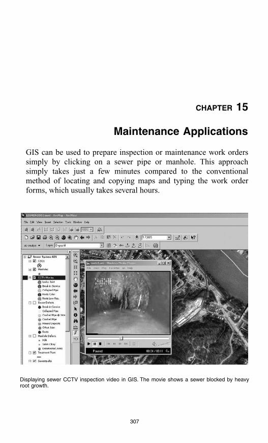
307
CHAPTER 15
Maintenance Applications
GIS can be used to prepare inspection or maintenance work orderssimply by clicking on a sewer pipe or manhole. This approachsimply takes just a few minutes compared to the conventionalmethod of locating and copying maps and typing the work orderforms, which usually takes several hours.
Displaying sewer CCTV inspection video in GIS. The movie shows a sewer blocked by heavyroot growth.

308 GIS APPLICATIONS FOR WATER, WASTEWATER, AND STORMWATER SYSTEMS
LEARNING OBJECTIVE
The learning objective of this chapter is to understand GIS applications in inspectionand maintenance of water, wastewater, and stormwater systems.
MAJOR TOPICS
• Field inspections• Asset management• GASB 34 applications• Wet-weather overflow management applications• CCTV inspections• Video mapping• Thematic mapping of inspection data• Work-order management• Identifying valves to be closed for repairing or replacing broken water mains• System rehabilitation and repair• Case studies
LIST OF CHAPTER ACRONYMS
AM/FM/GIS Automated Mapping/Facilities Management/Geographic InformationSystem
AVI Audio Video Interleaved (digital movie format)CCTV Closed-Circuit TelevisionCD Compact DiscCMMS Computerized Maintenance Management SystemDVD Digital Versatile DiscGAAP Generally Accepted Accounting PrinciplesGASB Government Accounting Standards BoardHTML Hyper Text Markup Language (a file extension)MPEG Moving Picture Experts Group (digital movievideo format)O&M Operation and MaintenancePDA Personal Digital Assistant (electronic handheld information device)PDF Portable Document Format (Adobe Acrobat)ROM Read Only MemoryVCR Video Cassette RecorderVHS Video Home System (video cassette format)
This book focuses on the four main applications of GIS, which are mapping, monitor-ing, modeling, and maintenance and are referred to as the “4M applications.” In this chapterwe will learn about the applications of the last M (maintenance).
To fully appreciate the benefits of GIS-based inspections, consider the followinghypothetical scenario. On March 10, 2004, following a heavy storm event, a sewer

MAINTENANCE APPLICATIONS 309
customer calls the Clearwater Sewer Authority to report a minor basement floodingevent without any property damage. An Authority operator immediately starts theGIS and enters the customer address. The GIS zooms to the resident property andshows all the sewers and manholes in the area. The operator queries the inspectiondata for a sewer segment adjacent to the customer property and finds that a minimovie of the closed-circuit television (CCTV) inspection dated July 10, 1998, isavailable. The operator plays the movie and sees light root growth in the segment.A query of the maintenance history for that segment shows that it has not beencleaned since April 5, 1997. This information indicates that the roots were nevercleaned and have probably grown to “heavy” status. The operator highlights thesewer segment, launches the work-order module, and completes a work-order formfor CCTV inspection and root removal, if necessary. The export button saves thework-order form and a map of the property and adjacent sewers in a PDF file. Theoperator immediately sends the PDF file by e-mail to the Authority’s sewer cleaningcontractor. The entire session from the time the customer called the Authority officetook about 30 min. The operator does not forget to call the customer to tell him thata work order has been issued to investigate the problem.
BUNCOMBE COUNTY’S SEWER SYSTEM INSPECTION AND MAINTENANCE
During the 1990s, the Metropolitan Sewerage District (MSD) of BuncombeCounty (North Carolina) spent more than $111 million rehabilitating the mostproblematic sewer lines in its system. MSD’s aggressive sewer rehabilitationprogram has successfully implemented numerous rehabilitation technologies. In1999, MSD began assessing a method of comprehensive basinwide rehabilitation.In this approach, every pipe in a drainage basin was evaluated using CCTV footageand engineering analysis. After evaluating this comprehensive basinwide rehabil-itation method for 4 years, MSD determined that it is overly time- and capital-intensive. Seeking a more efficient and quicker method to fix the system, MSDdeveloped and implemented a new GIS-based rehabilitation method called “piperating.”
The pipe rating method has five main elements: (1) CCTV information, (2) adefect scoring system, (3) GIS database software, (4) sanitary sewer overflow (SSO)history, and (5) engineering analysis. These components are combined to generatespecific projects for problem lines. Each structural defect noted in the video inspectionis given a defect score, in accordance with MSD’s standardized scoring system. Forexample, a circumferential crack is given a score of 20, and a collapsed pipe isassigned a score of 100. Defects are then embedded within the GIS database, withappropriate scores attached. Upon quantifying all structural defects within a pipesegment, three defect ratings are generated in the GIS: (1) peak defect rating, (2)mean defect rating, and (3) mean pipeline rating. These ratings allow users to visualizethe severity of pipe defects using GIS. Figure 15.1 shows an ArcGIS screenshot ofmean pipeline ratings. Such maps are used in prioritizing pipe segments for repairwork. They are also used to determine when several point repairs should be made to

310 GIS APPLICATIONS FOR WATER, WASTEWATER, AND STORMWATER SYSTEMS
a line as apposed to excavating the entire line (Bradford et al., 2004). Additionalinformation about this application is provided in Chapter 17 (Applications Sampler).
ASSET MANAGEMENT
As discussed in Chapter 14 (AM/FM/GIS Applications), at present our water andwastewater infrastructure, especially in the older cities, is in critical stages of deteri-oration and has started to crumble. Nationally and internationally, aging water andwastewater infrastructure is imposing enormous costs on local communities (Boothand Rogers, 2001). In the U.S., cities and utilities are demanding billions of dollarsof government grants and funds for renovating their water infrastructure. Due to an“out-of-sight, out-of-mind” philosophy and the lack of funds to follow a preventivemaintenance practice, the replacement is mostly performed on a react-to-crisis basis.A crisis maintenance program only corrects infrastructure problems after they havehappened. Notwithstanding the conventional wisdom, this reactive approach may notbe the best strategy as substantial expenditure and inconvenience can be avoided byreplacing a deteriorated pipeline before it actually breaks. A preventive maintenanceprogram is proactive because it strives to correct a problem before it occurs.
For water and wastewater systems, asset management can be defined as managinginfrastructure capital assets to minimize the total cost of owning and operating themwhile delivering the service levels customers desire (Booth and Rogers, 2001). Atypical asset management system has five components (Doyle and Rose, 2001):
Figure 15.1 ArcGIS screenshot of mean pipeline ratings for the Metropolitan Sewerage District(MSD) of Buncombe County, North Carolina.

MAINTENANCE APPLICATIONS 311
1. Facilities inventory: Describes each system element in an asset group. GIS canbe very useful in completing this task.
2. Condition assessment: Classifies each asset according to its capability to performthe intended function.
3. Valuation: Assigns a financial value to inventoried assets consistent with GenerallyAccepted Accounting Principles (GAAP).
4. Operations, maintenance, repair, and replacement management: Arguably the heartof a management system, this component tracks and records data about workorders and customer complaints, issues and tracks preventive and predictive main-tenance schedules, and generates crew assignments and work-site maps. GIS hasextensive capabilities to fulfill this part.
5. Analysis and evaluation: Considered as the brains of an asset management system,this component prioritizes work effort, analyzes cost-effectiveness, and optimizesasset performance.
An asset management system helps predict the future condition of assets andmajor rehabilitation costs for planning purposes. An effective asset managementsystem can reduce the cost of system operation and maintenance (O&M). Everysuccessful maintenance program should begin with an accurate system map becauseit is difficult to maintain a system if the users do not know where the water or sewerlines are. A well-constructed GIS should be used to create the system map. Historicalmaintenance data should also be linked with the GIS because it is difficult to schedulemaintenance when you do not know the last time it was done (Gaines, 2001). AGIS-based asset management system can be used as a decision support system forcapital improvement planning (CIP). For example, CH2M HILL (Atlanta, Georgia)used ESRI’s MapObjects GIS software to develop an infrastructure capital assetmanagement (ICAM) toolkit that can be used in a Web-based browser/server orstand-alone computing environment (Booth and Rogers, 2001).
In many cases, through more effective planning and management of infrastruc-ture improvements and system operations, organizations can realize annual savingsof 20 to 40% (Stern and Kendall, 2001). Boston Water and Sewer Commission(BWSC) has approximately 27,500 catch basins. In 2000, BWSC started enhancingits asset management program for locating, inspecting, and maintaining its catchbasins. BWSC improved the productivity and efficiency of its catch basin preventivemaintenance program by integrating it with GIS and a computerized maintenancemanagement system (CMMS). In lieu of using global positioning system (GPS), thecrews determined the precise location of catch basins by using a measuring wheelto measure distance from known points to the basin’s center. BWSC utilized hand-held touch-screen computers in the field to collect geographic location informationand more than 25 attributes. GIS data in Shapefile format and a GIS interfaceprovided the backbone of this application. The traditional paper-based data collectionmethods typically averaged 24 catch basin inspections per day, but the GIS-basedmethod boosted this rate to approximately 42 per day.
Boston Water and Sewer Commission’s GIS-based field-data-collection approachincreased the catch basin mapping productivity by more than 40% compared with tradi-tional, paper-based data collection methods (Lopes et al., 2002).

312 GIS APPLICATIONS FOR WATER, WASTEWATER, AND STORMWATER SYSTEMS
In the U.S., two key drivers are motivating improved asset management practicesin water and wastewater utilities: (1) GASB 34 requirements, and (2) wet-weatheroverflow requirements.
GASB 34 APPLICATIONS
In 1999, the Government Accounting Standards Board (GASB) issued Rule 34(known as GASB34) to govern financial reporting requirements of approximately85,000 state and local governments in the U.S. Considered the most significantchange in the history of government financing reporting in the U.S., GASB 34requires the cities to adequately account for and report their capital asset inventoryin a complete, accurate, and detailed manner (Booth and Rogers, 2001). The capitalassets include infrastructure networks such as roads, bridges, and water, wastewater,and stormwater systems.
The literature indicates that a GIS-based approach saves time spent in locating,organizing, and confirming the accuracy of field inspection information (Criss,2000). Industry experts believe that utilities can cut their maintenance costs in halfby implementing GIS-based preventive maintenance programs. Thus, integration ofGIS and maintenance management software is a natural progression for GIS appli-cations in the water and wastewater industry. For instance, the Wastewater CollectionDivision of Fairfax County, Virginia, linked the county’s sewer maps with thesanitary sewer maintenance management system database, making it easier to accessmaps during field activities (Fillmore et al., 2001). The City of Denver, Colorado,linked the city’s sewer system GIS to an information management system to effi-ciently track and manage maintenance operations (Gaines, 2001).
WET WEATHER OVERFLOW MANAGEMENT APPLICATIONS
Management of wet weather overflows is a fertile field for GIS technology. Byusing geographic information in mapping, facilities management, and work ordermanagement, a wastewater system manager can develop a detailed capital improve-ment program or operations and maintenance plan for the collection system.
Broken and damaged sewers, laterals, and manholes usually contribute signifi-cant amounts of wet weather inflow and infiltration (I/I) to a wastewater collectionsystem. This contribution often results in combined sewer overflows (CSO) fromcombined sewer systems and sanitary sewer overflows (SSO) from sanitary sewersystems.
In the U.S., CSO discharges are regulated by U.S. EPA’s National CSO Policy.The policy requires a System Inventory and Physical Characterization report. Majorportions of this report can be completed using GIS. The CSO policy’s Nine MinimumControls (NMC) mandate proper operation and regular maintenance programs forthe sewer system and CSO outfalls that can also benefit from inspection and main-tenance applications of GIS. SSO discharges are being regulated by U.S. EPA’s SSOrule that requires implementation of a Capacity, Management, Operations, and
MAINTENANCE APPLICATIONS 313
Maintenance (CMOM) program. CMOM requires the system owners/operators toidentify and prioritize structural deficiencies and rehabilitation actions for eachdeficiency. CMOM requirements offer a dynamic system management frameworkthat encourages evaluating and prioritizing efforts to identify and correct perfor-mance-limiting situations in a wastewater collection system. CMOM is a combina-tion of planning tools and physical activities that help communities optimize theperformance of their sewer systems. CMOM requirements mandate that the systemowner/operator properly manage, operate, and maintain, at all times, all parts of thecollection system. The owner/operator must provide adequate capacity to conveybase flows and peak flows for all parts of the collection system. CMOM requirementsinclude “maintaining a map” (Davis and Prelewicz, 2001), which is the simplestapplication of GIS as described in Chapter 9 (Mapping Applications).
Some wet weather overflow management experts believe that use of GIS is a must forCMOM compliance.
AutoCAD Map GIS Application for CMOM
The Stege Sanitary District (SSD) located near San Francisco Bay serves apopulation of approximately 40,000 in a 5.5 mi2 area. The goal of a CMOM programis the ultimate elimination of any type of overflow from the sanitary sewer system.SSD was challenged with the goal of “no overflows” in 1996. To meet this goal, anew maintenance model was implemented for sanitary sewers that used AutoCADMap GIS and Microsoft Access database software to identify system conditionscausing overflows, and prompted immediate action to correct problems via repairor replacement. Those lines showing the greatest damage and whose repair orreplacement were within the budget constraints established by the District, wouldbe immediately set right. The ability to make effective and economic decisionsregarding the capital replacement needs of the system based on the actual degradationof the system provided a degree of asset management that had not been readilyavailable to the management. The SSD experience indicated that proactive mainte-nance provides the most cost-effective means of managing the system to achievethe goal of “no overflows.”
During 1992 to 1994, SSD created the sewer and manhole layers in AutoCADformat and linked the capacity model output to these layers to identify line segmentsthat were overloaded. Complete GIS capability was added later with the use ofAutoCAD Map, an extension of the common AutoCAD drafting program that addsthe feature of linking information from external databases. During 1994 to 2001,information was collected in a database on the physical system characteristics,system hydraulic performance under selected flow conditions, system overflows,routine maintenance activities, CCTV inspections, and repairs and replacements. Alldatabase information was linked to the mapped line segments, thereby allowing aneasy evaluation of problem distribution throughout the system with a textual andgraphical response from the database query. The relational database program used

314 GIS APPLICATIONS FOR WATER, WASTEWATER, AND STORMWATER SYSTEMS
was Microsoft Access, which is compatible with AutoCAD Map. All of the workwas completed on a desktop PC (Rugaard, 2001).
CCTV INSPECTION OF SEWERS
Traditionally, municipalities have relied on analog video for internal inspectionof sewers. In this technique, remote-controlled and self-propelled cameras movethrough sewer lines to record the pipe’s internal conditions on a video tape. In aparallel operation, technicians create paper logs identifying the location, size, andother key information about the pipe. Referred to as CCTV inspection, this methodhas been considered to be the most effective and economical method of pinpointingthe sources of I/I contribution. For instance, by the late 1990s the City of Boston,Massachusetts, had conducted 12 million ft of CCTV inspection on video tapes.Using an inspection cost of one dollar per foot, the cost of collecting this informationcould be at least $12 million. CCTV inspection videotapes contain a wealth of usefulinformation about the state of a collection system, yet they have been often treatedas single-use items. A lot of money is spent on video inspections, yet inspectiondata are frequently underutilized mainly because accessing the information from theconventional video tapes and paper inspection log sheets has been difficult and timeconsuming (Criss, 2000).
GIS can be used as a document management system for CCTV inspection data.For example, users can click on a rehabilitated sewer pipe to see the “before” and“after” movies on their computer screen. This application, however, requires con-verting VHS video tapes to computer files (digital movies). Once converted andstored on computers, the valuable information once hidden in videotapes can beretrieved with the click of a mouse, eliminating the need for other equipment (TV,VCR, and cables) and office space to house the equipment. CDs take up 70% lessshelf space than VHS tapes. As a side benefit, digital movies can be used to createmultimedia presentations for utility management when requesting maintenance andrehabilitation funds. After all, a video is worth a thousand pictures. Most video tapeshave a short shelf life of approximately 10 years and their video quality and perfor-mance are inferior to digital media. Unlike VHS tapes, digital videos do not losepicture quality when copied. Digital technology also allows high-resolution snap-shots of defective pipe segments taken from the video. Dynamic segmentation andimage integration features allow storage and display of these images with footagereading and a description of the pipe defect. For benefits like these, experts predictthat by 2008, approximately 90% of wastewater utilities will be using digital videotechnology (Bufe, 2003).
As stated in the preceding text, integrating CCTV videos with GIS requiresmigrating from video tapes to digital movies. Four migration methods are possible:
1. Convert existing video tapes to digital files2. Digitize existing video tapes3. Retrofit tape systems with digital systems4. Record directly in digital format

MAINTENANCE APPLICATIONS 315
Convert Existing Video Tapes to Digital Files
In this method (which is the simplest), the existing video tapes are converted tomultimedia computer files in the AVI or MPEG format. The hardware required forthis method includes TV, VCR, multimedia computer, CD or DVD burner, and avideo capture card. Video capture cards allow display of TV or VCR output on acomputer screen. Some multimedia computers have built-in (internal) video capturecards. If an internal card is not installed, an external card that typically costs a fewhundred dollars should be used. A video capture and editing software, which typi-cally comes with the card, is also required. Figure 15.2 shows a screenshot of DigitalVideo Producer, a video capture software from Asymetrix Corporation.
The TV is connected to the VCR, and the VCR is connected to the video capturecard (if external) or the computer (if internal) using AV cables. When a tape is playedin the VCR, the user sees the video on the TV and on the computer screen. Thevideo capture software has a VCR-like console with play, stop, and record buttons.When the user clicks on the software’s record button, usually at the beginning of asewer defect (e.g., collapsed pipe, root growth, break-in lateral, etc.), the computerstarts to record the video in a computer file, usually in AVI or MPEG format. The
Figure 15.2 Screenshot of Digital Video Producer’s video capture capability.

316 GIS APPLICATIONS FOR WATER, WASTEWATER, AND STORMWATER SYSTEMS
file recording stops when the STOP button is clicked, usually at the end of the sewerdefect. Instead of converting the entire video tape, generally 5 to 30 sec mini moviesshowing problem areas are captured because the resulting files can be very large.For example, a 5 to 15 sec video segment recorded in color with sound can be 30to 60 MB in size. Sound can be turned off to reduce the file size. Finally, in orderto free up the computer hard disk space, the recorded digital movies are copied todigital media (e.g., CD-ROM or DVD-ROM). Raw video files can be compressedto optimize disk space. A CD cannot store more than 15 to 30 min of uncompresseddata. However, in compressed format such as MPEG-1 or MPEG-2, 1 to 1.5 h ofvideo can be stored on a CD and 6 to 12 h on a DVD. Figure 15.3 shows a samplemini movie in AVI format showing a collapsed pipe.
Digitize Existing VHS Tapes
This is basically a more efficient and automatic implementation of the previousmethod. Special video software is used for compressing and indexing video tapes todigital media. For example, the Tape-to-CD module of flexidata pipe survey reportingsoftware from Pearpoint, Inc. (Thousand Palms, California), uses advanced optical char-acter recognition (OCR) technology to read the footage count displayed on the monitor
Figure 15.3 Sample mini movie in AVI format showing collapsed sewer pipe.

MAINTENANCE APPLICATIONS 317
screen. This product was designed using skills and expertise gained in the developmentof automatic recognition of vehicle license plates. It allows the Pearpoint system toprovide indexing of sewer records against the footage shown on the original videotape.The resulting CD will not only contain the original real time video but also a report.
WinCan
WinCan from WinCan America, Inc. (Durango, Colorado), is another exampleof video software that allows the user to capture either videos or pictures. Picturesmay be captured in several different formats such as JPG or BMP. Mini movie filescan also be created in increments of 5 to 35 sec. Videos may be captured in severaldifferent formats, including the most common, MPEG and AVI. WinCan can inte-grate stored pictures, live video from the camera or VCR, and stored movies in thepipe inspection database. Figure 15.4 shows a screenshot of the WinCan interface.The left window lists the inspected pipes in the WinCan project database. The rightwindows shows the mini movies for the selected pipes. The bottom window displaysthe observed defects for the selected pipe. WinCan also allows personal digitalassistant (PDA)-based manhole reporting. The PDA (e.g., an iPAQ or PalmPilot) isused in the field to gather data with the user standing above the structure. A cus-tomized WinCan software is added to the user’s PDA. Pull-down menus and easyfill-in fields make gathering the data as easy as using the full WinCan software.Back in the office, the user HotSyncs the PDA with the computer and the informationis simply added to WinCan (WinCan, 2001).
WinCan interacts with GIS packages in two ways: (1) interfaces with the GISdatabase and (2) updates the GIS database. In the first method, the WinCan databaseinterfaces with the GIS database by using a metadatabase. This metadatabase con-tains information from WinCan projects, such as unique manhole identifiers, linesection numbers, street names, and pipe sizes. When a GIS user attempts to accessa particular feature (e.g., a manhole or line segment), the software searches themetadatabase to determine if the feature is available. If an associated WinCan reportis available, the software opens the report and highlights the specific item. The usercan then display associated pictures, videos, or inspection data. This method requirestoggling between WinCan and the GIS software. In the second method, an externalutility appends the WinCan data to the GIS database. GIS users can then select thelocations in their maps and view WinCan database and associated graphics withoutstarting the WinCan program (Criss, 2000).
Retrofit Tape Systems with Digital Systems
The typical cameras on board the CCTV inspection vehicles are adequate foruse in digital applications. Most simply need the addition of a compression unit toconvert their analog signals to a digital format. In this method, digital video pro-cessing hardware and software are installed in the CCTV inspection vehicle andlinked to an existing tape system.
Pearpoint equipment users can interface the Pearpoint hardware directly withWinCan. This eliminates the need for a separate overlay system with encoder.
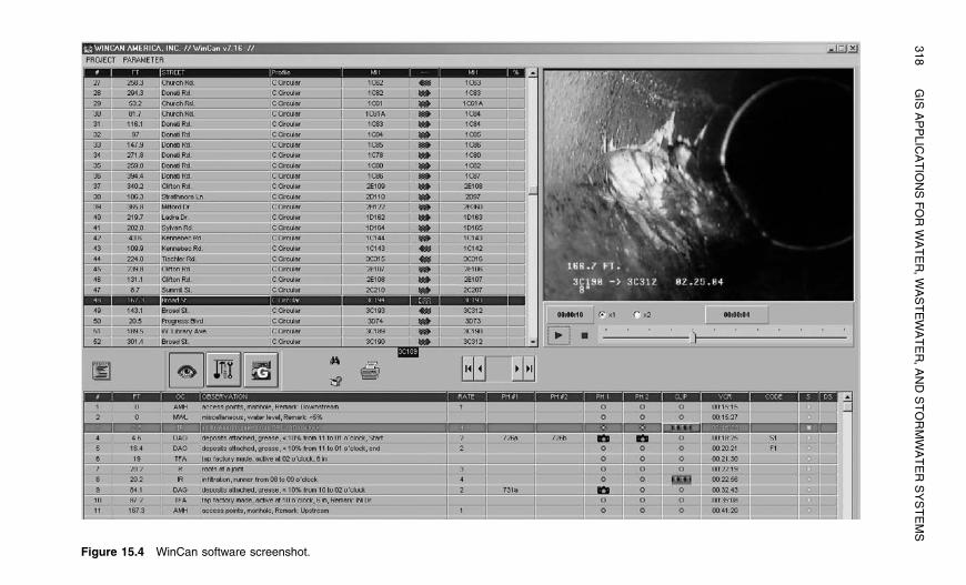
318G
IS A
PP
LICA
TIO
NS
FO
R W
AT
ER
, WA
ST
EW
AT
ER
, AN
D S
TO
RM
WA
TE
R S
YS
TE
MS
Figure 15.4 WinCan software screenshot.

MAINTENANCE APPLICATIONS 319
According to Pearpoint, the installation is much easier with no hardware integrationand wiring/soldering necessary. Camera inclination and other Pearpoint featuresfunction instantly with appropriate setup.
Another example of this approach is the PipeTech™ Software Suite from Penin-sular Technologies, Inc. (Ada, Michigan). PipeTech is an innovative solution forsimplifying sewer inspection projects. It allows collection, editing, analysis, andarchiving of all inspection data digitally, eliminating the need for VHS tapes andthe stacks of paper attachments that normally accompany an inspection project.PipeTech’s Scan product is an on-site solution for video recording and incidentreporting. Scan captures and compresses video in real time and facilitates the record-ing of incident locations. Incidents are entered on an electronic log sheet and areautomatically cross-referenced with their occurrences in the video. Scan eliminatesthe need for a TV, VCR, and VHS tapes in the video vehicle. Videos captured usingScan are clearer than those captured through a VCR (PipeTech, 2000).
Video software such as WinCan and PipeTech also provide an on-screen pipelineor a video viewer for retrieval of stored images and movies. Consisting of a linesegment graphic, these utilities allow the user to scroll along a line segment and displayobservations, photos, or movies by clicking on any desired location. An example isshown in Figure 14.3 for Hansen’s Infrastructure Management System. This is possiblebecause the defect location is cross-referenced with the video. In addition to the typicalstop, play, and pause controls, video step and loop controls help the user to directvideo progression. Seeking to any instant of video is also possible.
Record Directly in Digital Format
In this method, no VHS tapes are involved at all. The sewer inspection video isrecorded directly in onboard computers as digital movies, using digital cameras.This method requires installation of appropriate digital recording hardware in theCCTV vehicle. For example, Pearpoint manufactures several video pipeline inspec-tion systems with digital color video cameras.
This system offers complete integration of data and video. It enables a technicianto watch the video as it is recorded and flag the video for defects in real time. Userscan then jump to the flagged video frames without searching through the entire video(Bufe, 2003).
Linking Digital Movies to GIS
The digital movies created by using one of the preceding methods should belinked to the sewers layer in the GIS database. This will enable users to click on asewer line in the GIS map to display the digital movie of the sewer defect. Thefollowing steps should be performed to accomplish the linkage in ArcView 3.x:
1. Add a new field to the sewer layer table to store the movie filename. Figure 15.5ashows an ArcView 3.2 database table for sanitary sewers containing a field named“Movie” for holding the movie filenames.
2. Enter the video filename for each sewer segment for which a movie is available.

320 GIS APPLICATIONS FOR WATER, WASTEWATER, AND STORMWATER SYSTEMS
3. Write an Avenue script (shown in Figure 15.6 and described in the following text)for displaying the movie.
4. In the “Theme Properties” dialogue box for the sewers theme, click on the “HotLink” tab as shown in Figure 15.6. Set “Field” to the field created in Step 1, set“Predefined Action” to “Link to User Script,” and set “Script” to the scriptdeveloped in Step 3.
5. Pick the Hot Link tool (the lightning bolt) shown in Figure 15.6 from the tool barand click on a pipe with a video file to launch the digital movie.
Figure 15.6 shows a sample script called “Movie&ImageHotLink” for displayingmovie files. The code of the script is included in Chapter 1 (GIS Applications,Applications Programming section).
The successful linkage of movies to sewers requires that both the CCTV inspec-tion data and the sewer database table in the GIS have a common ID. This wouldessentially require planning ahead before conducting CCTV inspections to makesure that the inspection crews use the GIS IDs in their inspection reports. As analternative to linking videos to sewers, a point layer can be created for video locations.Figure 15.5b shows an ArcView 3.2 point database table for CCTV movie locations.It has three fields for entering movie filenames. The users can enter the video filenameand path separately in the AVI and Path fields. Or, an absolute pathname can be
Figure 15.5 Linking digital movies to ArcView GIS. Above (a) linkage to sewers; below (b)linkage to points.

MAINTENANCE APPLICATIONS 321
entered in the VideoFile field. The disadvantage of absolute pathnames is that theapplication will not work if the pathname becomes invalid when video files aremoved to another location (e.g., a CD or network drive). Here the users can clickon a video point to see the digital movie.
In ArcGIS, the video files can be displayed without a script using the Hyperlinktool, which also looks like a lightning bolt. As in ArcView 3.x, the movie filenameis entered in a database field. When the end of the bolt is near a defective sewer,the hyperlinked filename is displayed if the file exists. Clicking on the sewer willlaunch the movie. The hyperlinking is configured by right-clicking on the sewerlayer, selecting properties, and then the display tab. The figure on the first page ofthis chapter shows a digital movie being played in ArcGIS 8.2.
VIDEO MAPPING
Today, GIS map features can be linked to any kind of file to document inspectionof a location through pictures, field notes, audio, streaming video, etc. When digitalvideo, GPS, and GIS maps are combined, the possibilities are limited only by theuser’s imagination.
Traditionally, GIS users have employed a low-tech and cumbersome approachto associate an inspection picture (e.g., inside of a sewer manhole) or video withits location. This method involves taking pictures (or recording video), writingthe pictures’ (or video’s) description and frame numbers, scanning the pictures(or converting the video from analog to digital format), collecting GPS coordinatesof picture locations, and entering all this information in the GIS database. In today’s
Figure 15.6 ArcView GIS Hot Link Tool for linking sewer movies to sewer pipes.

322 GIS APPLICATIONS FOR WATER, WASTEWATER, AND STORMWATER SYSTEMS
information age, this method is error prone and inefficient. The high-tech alternativeknown as video mapping (or media mapping) refers to georeferencing video footageby associating GPS data with video (Pfister et al., 2001). A GIS software can thenread the GPS locations referenced to video time codes into its database. A map ofvideo locations is created that can be clicked by the users to access the desired videofootage. Video mapping technology can be applied to document sewer inspectionsand smoke-testing in GIS maps (Murphy, 2000).
Video mapping integrates GPS data and GIS maps to create interactive multimediamaps without manual scanning of photos or data entry into a computer.
Multimedia Mapping System (MMS) and Video Mapping System (VMS) soft-ware programs from Red Hen Systems, Inc. (Fort Collins, Colorado), are typicalexamples of video mapping products. VMS is a self-contained GPS encoder thatrecords all data types — video, audio, and GPS — on a single tape. Users collectvideo, location, and audio information at the same time. It contains an integratedGPS receiver that receives location coordinates from satellites and then convertsthem to an audio signal for storage on video tape (Morrison and Ruiz, 2001). Theuser attaches the product to a video camera and records the field inspections. VMSsends GPS data from its internal receiver to the camera’s microphone input. Afterrecording the video, the user connects the system to a computer with Red Hen’sMediaMapper software installed. VMS then sends the data to the computer to createa video map in TAB, SHP, or HTML format. These maps allow the users to clickand view still images or video clips, play audio files, or display documents or datasets. MMS integrates the VMS unit and its built-in GPS receiver with a GPS antenna,headphone, and microphone.
MediaMapper software provides basic GIS functions and enables users to linkgeoreference audio and video clips to GIS features. This functionality is essentiallysimilar to ArcView’s Hot Link tool described in the previous section but it is enabledby MediaMapper automatically. Software extensions are available for accessingMediaMapper data in MapInfo and ArcView GIS packages.
THEMATIC MAPPING OF INSPECTION DATA
Some applications use information from several different databases or tables.For example, a smoke-testing application might require information from the man-hole and customer account databases. It is inefficient and cumbersome to enter thedata from different tables in one table. Relational database tables allow accessinginformation from different tables without physically joining them.
A relational database stores information in records (rows) and fields (columns)and conducts searches by using data in specified fields of one table to find additionaldata in another field. This capability allows linking two tables that have a commonfield. The common field can be used to link the GIS feature tables to virtually anyexternal database table. This linkage capability allows the GIS to make effective useof existing databases without requiring additional data entry in the GIS database.

MAINTENANCE APPLICATIONS 323
Once the GIS and external database tables have been linked, the external data canbe queried or mapped from within the GIS.
Typical manhole inspection reports have valuable attributes, such as:
• Structure number• Street name• Inspection date• Offset from curb• Structure type• Cover or grate diameter• Number of holes in the cover• Frame adjustment type• Corbel type• Manhole wall type• Manhole area• Depth of structure• Bricks missing (Yes/No)• Ladder rungs (Yes/No)• Ladder rungs condition• Apron leaking (Yes/No)• Pipe seals leaking (Yes/No)• Manhole wall leaking (Yes/No)• Catch basin connected (Yes/No)• Root intrusion (Yes/No)• Joint deterioration (Yes/No)
A manhole theme table can be linked to a manhole inspection table to createthematic maps of manhole conditions, which are excellent decision support tools forscheduling maintenance and inspection activities. The linkage can be created easilyas long as both the inspection reports and the GIS database use the same manhole IDs.
Figure 15.7 shows the linkage of a manhole theme table in ArcView with theexternal manhole inspection table. The linkage is accomplished using the fields“Mhid” of the manhole theme table and “Mh_id” of the manhole inspection table.When the manhole “MH9-2” is selected in the GIS theme table, correspondingrecords in the manhole inspection table are also selected. Figure 15.8 shows athematic map of manhole joint defects based on the “Joint Deterioration” attributeof the manhole inspection report created by using the table-linkage approach.
Similarly, typical CCTV inspection logs also have valuable attributes, such as:
• Date televised• Type of pipe• Begin and end manhole• Total footage televised• Overall pipe condition• Manhole condition• Joint spacing• Joint alignment• Number of houses• Remarks

324 GIS APPLICATIONS FOR WATER, WASTEWATER, AND STORMWATER SYSTEMS
Using the method described in the preceding text, the CCTV inspection logs can beintegrated with the GIS database. This allows creation of thematic maps of sewerconditions. As described earlier, the successful linking of GIS features and inspectiondata requires that both the GIS database and the inspection data have a common ID.
Figure 15.7 Linking manhole theme table and external manhole inspection table in ArcView.
Figure 15.8 Thematic map of manhole joint defects.

MAINTENANCE APPLICATIONS 325
Figure 15.9 shows a thematic map of pipe defects based on the “Remarks”attribute of the CCTV inspection logs, which contained information about sewerdefects such as root growth, collapsed pipes, leaks, break-in service, etc.
WORK ORDER MANAGEMENT
Although this section focuses on wastewater system work orders, the method-ology is equally applicable to water and stormwater systems.
Conventional work order management requires searching and printing theappropriate sewer system maps and manual completion of paper forms. GIS canbe used to prepare work orders simply by clicking on the desired sewer or manholein the GIS map. When the user clicks on an object, a work order inspection formis displayed that the user can fill by entering work information or by selectingpredefined actions from drop-down lists. The completed work-order form and
Figure 15.9 Thematic map of pipe defects.

326 GIS APPLICATIONS FOR WATER, WASTEWATER, AND STORMWATER SYSTEMS
corresponding map area can be printed for the inspection and maintenance crews.The entire process takes just a few minutes compared to the conventional methodof locating and copying maps and typing the work order forms, which usually takesseveral hours.
GIS-based work-order management requires automated mapping/facilities man-agement (AM/FM) software extensions that can be run from within the GIS soft-ware. These add-on programs, referred to as AM/FM/GIS software, are describedin Chapter 14 (AM/FM/GIS Applications). AM/FM/GIS systems are especiallyuseful for asset inventory, inspection and maintenance, and work management(Shamsi and Fletcher, 2000). The Cityworks (formerly Pipeworks, Azteca Systems,Sandy, Utah) AM/FM/GIS software suite includes ArcView and ArcGIS extensions,which help users integrate their GIS and work management. Its Wastewater Modulecan be used for inspection and maintenance of sewer systems and for managingand recording a CCTV inspection program for sewers. Cityworks Work Ordermodules are used to create and manage work orders for inspections and tests, andfor detailed inventory for water and sewer systems. The Cityworks work manage-ment solutions are based on a GIS-centric approach. Cityworks does not treat theGIS as subordinate to the work management system. Instead of integrating the workmanagement system with the GIS, it uses the GIS as a work management system(Azteca, 1999). Figure 15.10 shows the Cityworks work order management screenfor CCTV inspection of sewers.
Figure 15.10 Cityworks work order management screen for CCTV inspections.
MAINTENANCE APPLICATIONS 327
WATER MAIN ISOLATION TRACE
In many cases, the labor and material costs for fixing a broken water main aresmaller than the hidden costs resulting from the pipe break. The hidden costsmight be incurred due to human injury, property damage, litigation, customerinconvenience, traffic delays, police and emergency services, lost economic oppor-tunities, and diminished fire-fighting capacity in other parts of the system. GISoffers many applications in the inspection and maintenance of water distributionsystems. Water main isolation trace is one such application.
When a water main breaks, it should be isolated from the rest of the waterdistribution network for repairing the break or replacing the pipe. Water mainisolation trace is defined as identifying those water distribution system valves thatmust be closed to repair or replace a broken water main. A water distribution systemnetwork layer that “knows” which links are connected to which nodes (i.e., hastopology) can be used to traverse networks (Haestad et al., 2003) for solving thewater main isolation problem. In addition to valve identification, GIS also allowsan advance analysis of various water main shutdown scenarios, such as:
• Refining the valve search based on inoperable valves• Identifying dry pipes (i.e., pipes without water)• Identifying the affected customers served by dry pipes• Identifying critical water service customers (e.g., hospitals), who need uninter-
rupted service• Determining the extent of a service interruption to avoid unintentional shutdowns• Capturing leak history data that are useful in pipeline replacement modeling
A GIS must have topology to benefit from the isolation trace application. Topol-ogy is defined as the spatial relationship between features. Spatial relationshipsbetween connecting or adjacent features, such as the pipes connected to a hydrant,which are so obvious to the human eye, must be explicitly defined to make thedigitized maps “intelligent.” For example, our eyes can instantly identify the pipeserving a house just by looking at a paper map. A GIS, on the other hand, mustmathematically compare the pipe and parcel layers to complete this task. Topologyis, therefore, defined as a mathematical procedure for explicitly defining spatialrelationships between features. The subject of topology is so sophisticated that it isconsidered a branch of mathematics (Shamsi, 2002). The GIS layers that havetopology can be used to trace transportation or utility networks. A water distributionsystem network layer that knows which links are connected to which nodes can beused to traverse networks (Haestad et al., 2003).
ESRI’s ArcMap software provides many network analysis functions. ArcMap’sstandard interface can be customized to add network analysis functions such as networktracing. For example, a sample toolbar called the Utility Network Analyst (UNA)was developed by ESRI to help ArcGIS users develop custom applications (ESRI,2002c). The UNA consists of a toolbar, a pull-down menu for saving and loadingflags and barriers and setting options, a set of tools for specifying flags and barriers,and a combo box containing the list of available trace tasks. The UNA toolbar hasa set of trace tasks (Find Connected, Trace Upstream, etc.) that can be used to solve

328 GIS APPLICATIONS FOR WATER, WASTEWATER, AND STORMWATER SYSTEMS
many problems. The Isolation Trace Task of the UNA toolbar takes a single specifiededge flag and determines the valves that would need to be turned off to isolate thearea. The UNA toolbar can be downloaded from http://arcobjectsonline.esri.com.The steps required to use the Isolation Trace Task are:
1. Register the trace task with Categories.exe as an ESRI Utility Network Task.2. Close and restart ArcMap.3. Add your network to ArcMap. Use the Add Edge Flag Tool on the Utility Network
Analyst toolbar to place an edge flag at the location you wish to isolate.4. Choose “Isolation Trace” from the list of available trace tasks and perform the
trace. The result will be a display of the isolated area and a selection set of thevalves to turn off.
CASE STUDIES
Representative case studies of GIS applications in maintenance are given in thefollowing subsections.
Isolation Trace Case Studies
Figure 15.11 shows an isolation trace example from the PipeWorks exampledata. Pipeworks (now known as CityWorks) is an AM/FM/GIS software packagefrom Azteca Systems (Sandy, Utah, www.azteca.com), that runs as an ArcViewExtension. The trace is conducted by selecting the broken water main (midway onthe pipe in the center of the map) and clicking on the “Isolation Trace” button. Thetop screenshot shows that four valves must be closed to isolate the broken watermain for repair or replacement. Next, it was assumed that one of these four valveslocated at the bottom of the screen is “open inoperable,” which would prevent thisvalve from being closed down. This scenario was modeled by changing the valvestatus from “open operable” to “open inoperable.” The actual valve status can bemade available in the GIS database if field inspections data are integrated with it.The bottom screenshot shows that due to the inoperable status of one of the valves,two additional (i.e., a total of six) valves must be closed.
In 2001, San Jose Water Company, which services the City of San Jose, Cali-fornia, created an ArcView 8.1 application called “Main Break” to accomplish thepreceding functions using Visual Basic and ArcObjects running against a personalgeodatabase. The application was installed at SJWC’s main office and on sevenlaptop computers. The laptop computers empowered the field personnel with amobile GIS that allowed on-site identification of the valves to be closed (Coates,2003).
Sewer System Inspections in Washington County
A sewer system inspection GIS was implemented for a small community locatedin the Washington County of Pennsylvania with a population of 4900 people and a

MAINTENANCE APPLICATIONS 329
1.5 MGD (million gallons per day) sewage treatment plant. This GIS project con-sisted of the following tasks:
1. Develop manhole and sewer line coverages2. Add manhole attributes from corrective action plan (CAP) manhole inspection
reports3. Add sewer attributes from CCTV inspection logs4. Develop service laterals coverage from CCTV inspection logs5. Develop video coverage from CCTV inspection tapes6. Add street names to the existing roads coverage7. Align image and feature themes8. Package the information for delivery
Figure 15.11 Isolation trace example. Above: all valves operable; below: one valve inoperable.

330 GIS APPLICATIONS FOR WATER, WASTEWATER, AND STORMWATER SYSTEMS
The project was completed in 2000 in 6 months for a cost of $15,000. Variousfree public-domain GIS data were used to keep the project cost low. These dataincluded USGS digital orthophoto quarter quadrangles (DOQQ), digital raster graph-ics (DRG), and digital elevation models (DEM). Tasks 3, 4, and 5 were accomplishedusing the various techniques described in this chapter. Fifty mini movies were createdfrom the existing VHS tapes and stored on five CD-ROMs. The movie files consistedof uncompressed AVI files of 40 to 60 MB size and resulted in approximately 3 GBof digital data.
Figure 15.12 shows various ArcView GIS themes of the project overlayed onthe DOQQ image. The figure on the first page of this chapter shows an ArcViewproject screen displaying a mini movie of root growth for a user-specified location.Figure 15.8 and Figure 15.9 presented earlier show thematic maps of manhole andsewer defects, respectively.
Sewer Rehabilitation in Baldwin
Facing stringent regulatory requirements at the turn of the century, many com-munities in the Allegheny County (Pennsylvania) started undertaking comprehensivesewer rehabilitation projects to reduce systemwide inflow and infiltration. Rehabil-itation activities included internal televising, pipe lining, pipe bursting, pipe replace-ment, manhole repair, and manhole replacement.
Baldwin Borough, a 5.5 mi2 municipality located in the Greater Pittsburgharea with a population of 22,000, undertook a similar project. Baldwin’s consultant,
Figure 15.12 ArcView layers created from sewer system inspections data.
MAINTENANCE APPLICATIONS 331
(Chester Engineers, Pittsburgh, Pennsylvania) developed a sewer rehabilitationdata management system (SRDMS) to assist in the planning and design phases ofBaldwin’s sewer rehabilitation projects. Initially, the system was successfullytested in the bidding phase for internal inspection of over 200,000 ft of sanitarysewers and 3,000 manholes. The system utilized digital map data compiled duringa sewer-mapping effort initiated in 1996. The project team field-verified the sewernetwork data based on CCTV inspections conducted during a 3-month period in2001. Concurrent with this effort, a Microsoft Access™ database was developedto capture conditional information for each surveyed sewer feature, apply unitcosts for all necessary repair work, and generate a variety of reports for use inbid document submittals. Subsequent rehabilitation projects proved the effective-ness of SRDMS, leading to its implementation in several Allegheny County com-munities.
SRDMS is a GIS-based system because it reads and writes the information in aGIS database. It utilizes a relational database (e.g., Microsoft Access) to managedisparate data related to rehabilitation work, including manhole inspections, televisedsewer line inspections, and flow data. This relational database is linked with the GISdatabase to facilitate mapping of the extent and severity of system damage and therecommended remedial activities. The required GIS layers can be created from avariety of sources, such as ArcInfo™ coverages, ArcView™ Shapefiles, and CAD files(e.g., Integraph™ or AutoCAD™). Preprocessing of CAD data to ensure the connec-tivity of sewer features may be necessary as the system requires that connectivitybe established between all lines and manholes. SRDMS can use field inspection datafrom the conventional paper forms or the latest digital data collectors (e.g., PDAs,or tablet PCs). The GIS interface was initially developed as an ArcView 3.2 Exten-sion. An ArcGIS version was created subsequently. SRDMS links inspection andrepair information contained in the Access database to the corresponding GIS fea-tures. Applications of this system have resulted in a 20 to 30% reduction in projectmanagement labor effort over traditional methods. SRDMS provides the end userwith the following functionalities:
• Provides the ability to visualize the overall condition of the sewage collectionsystem using thematic maps of problematic areas.
• Identifies the precise locations of specific rehabilitation activities based upon anengineering interpretation of CCTV and manhole inspection results.
• Develops budgetary pricing for system repairs and rehabilitation work. It generatescost estimates for manhole rehabilitation and line repair work by applying mul-tipliers to unit repair costs. Unit costs are entered by the project manager. Theunit cost estimates may be modified at any time. The system will automaticallyupdate all aggregate costs based on the updated figures.
• Provides a series of reports detailing system damage, recommended remedialaction, and cost estimates for the repair of damaged structures.
• Develops plans for distribution to prospective contractors during the biddingprocess.
• Provides a mechanism for tracking and reporting the progress of the rehabilitationactivities.

332 GIS APPLICATIONS FOR WATER, WASTEWATER, AND STORMWATER SYSTEMS
• Expands the content of the original GIS to include the location of service lateralconnections identified during the televising process.
• Corrects inaccuracies in the original GIS based upon information obtained duringthe televising process.
Figure 15.13 SRDMS line defect and repair entry form.
Figure 15.14 SRDMS line and manhole repair map.

MAINTENANCE APPLICATIONS 333
Figure 15.13 shows the SRDMS line defect and repair entry form. The left sideof this form receives input from the CCTV inspections database and automaticallyupdates the GIS layer for pipes. The right side of the form, which recommendsappropriate repairs, is completed by the project engineer or manager based onindividual judgment and experience. Manhole and line repairs recommended by theuser are added to the GIS as new layers. Figure 15.14 shows an ArcView screenshotof the line and manhole repair map. All the manholes targeted for repairs are clearlyshown as large dots. All the sewers targeted for spot repairs or full-length liningrepairs are shown in different colors.
USEFUL WEB SITES
CHAPTER SUMMARY
This chapter provided an overview of GIS applications for the fourth M of the“4M approach” in the inspection and maintenance of water, wastewater, and storm-water systems. These applications include asset management and field inspectionsrequired by regulations such as GASB 34 and wet-weather overflow policies in theU.S. GIS also allows integrating work-order management and video inspections(e.g., CCTV inspections of sewers) with maps, which results in workflow efficiencyimprovement and cost savings for water and wastewater utilities. GIS can be usedas a project management tool for system rehabilitation and repair work. Last but notleast, GIS allows thematic mapping of inspection data to enable effective commu-nication with decision makers and stakeholders. Real-world examples and casestudies presented in this chapter show that GIS can be used for more efficientinspection and maintenance of water, wastewater, and stormwater systems.
CHAPTER QUESTIONS
1. What is the “infrastructure problem,” and how can GIS help to solve this problem?2. What is asset management, and how can GIS help in asset management of water,
wastewater, and stormwater systems?3. Describe two examples of GIS applications in regulatory compliance for water,
wastewater, or stormwater systems.4. What is water main isolation trace? How will you implement it on a mobile device?
Azteca Systems www.azteca.comGovernment Accounting Standards Board (GASB)
www.gasb.org
Pearpoint, Inc. www.pearpoint.comPeninsular Technologies, Inc. www.pent.comRed Hen Systems, Inc. www.redhensystems.comWinCan America, Inc. www.wincanamerica.com


335
CHAPTER 16
Security Planning andVulnerability Assessment
Although water and wastewater systems are generally well preparedto deal with natural disasters and accidents, many utilities prior toSeptember 11, 2001 had given little consideration to defendingthemselves against acts of terrorism. Read this chapter to see howGIS can help in safeguarding your water and sewer systems againstthe acts of terrorism.
Water distribution systems are especially vulnerable to acts of terror.

336 GIS APPLICATIONS FOR WATER, WASTEWATER, AND STORMWATER SYSTEMS
LEARNING OBJECTIVE
The learning objective of this chapter is to understand GIS applications in securityplanning and vulnerability assessment of water and sewer systems.
MAJOR TOPICS
• GIS applications in planning• Security planning• Vulnerability assessment• Security modeling software
LIST OF CHAPTER ACRONYMS
AMSA Association of Metropolitan Sewerage AgenciesEPA (U.S.) Environmental Protection AgencyERP Emergency Response PlanOGC Open GIS ConsortiumVSAT Vulnerability Self Assessment Tool
GIS APPLICATIONS IN PLANNING
GIS technologies have enabled planning professionals to make better and fasterplanning decisions. New software advances have revolutionized the preparation anduse of master plans for water and sewer systems. GIS technologies provide variousplanning tools such as:
1. Remote-sensing data (described in Chapter 3)2. Land-use/land-cover data (described in Chapter 3, Chapter 11, and Chapter 12)3. Intelligent maps (described in Chapter 8 and Chapter 9)4. Hydrologic and hydraulic models (described in Chapter 11 to Chapter 13)
With the help of case studies and examples, this chapter will focus on how toapply these tools for security planning purposes.
CITY OF ALBUQUERQUE’S WASTEWATER MASTER PLAN
In 1990, the City of Albuquerque, New Mexico, began a multiphase planning effort toevaluate its existing wastewater conveyance and treatment facilities, project future growthand flows, create programs for monitoring and rehabilitating existing infrastructure, anddevelop an organized approach to ensuring that future facilities keep pace with develop-ment. The City used GIS technology to develop a 40-year master plan for its wastewatercollection and treatment system. The master plan was created by integrating the City’sGIS data with a number of other computer applications including demographic modeling,

SECURITY PLANNING AND VULNERABILITY ASSESSMENT 337
land-use mapping, hydraulic analysis, and infrastructure rehabilitation planning. The GISapproach enabled the City to create a master plan that could be easily updated in futureas new development takes place (American City & County, 1991).
SECURITY PLANNING
Water, wastewater, and stormwater systems face both natural (floods, droughts,earthquakes, fires, etc.) and man-made (terrorism, vandalism, sabotage, arson, cyberattacks, etc.) threats. Although water industry utilities have learned from naturaldisasters, their experience with human-caused threats is small (Grigg, 2002). Thebasic form of protection against attacks or threats of attacks is a security system.Security planning methods include hazard assessment, vulnerability assessment,mitigation, response planning, and crisis communications (Burns et al., 2001).Vulnerability assessment is an important step in disaster preparedness. In the U.S.,many utilities are performing mandatory vulnerability assessments.
When terrorists attacked the World Trade Center complex in New York and thePentagon building in Washington, D.C., on September 11, 2001, the U.S. witnessedone of the worst days of its 225-year history. The unfortunate event also witnessedthe best of the American spirit as people everywhere, including the GIS community,rushed to help. GIS supported response efforts at the World Trade Center and thePentagon by coordinating the search for survivors and identifying hazardous areas.Planning for collection of airborne imagery over Ground Zero began within hoursof the terrorist attack. Only 3 hours after the attack, France’s SPOT 4 satellite captured20-m resolution infrared images of the fires blazing in Manhattan. On September 12,Space Imaging’s IKONOS satellite acquired 1-m imagery of both the World TradeCenter area and the Pentagon (Barnes, 2001b). LIDAR* images collected on Sep-tember 19, 2001, at 5000 ft were used to create 3D depictions of the terrain andbuildings of the World Trade Center complex (Logan, 2002). The media, to coverthe stories related to the terrorist attack, frequently used these 3D renderings.
Since September 11, 2001, concerns over intentional contamination have resultedin new federal legislation in the U.S. requiring community water systems to developEmergency Response Plans (ERPs) (Haestad Methods, 2003a). In the Public HealthSecurity and Bioterrorism Preparedness and Response Act of 2002, U.S. Congressrecognized the need for drinking water system utilities to undertake a more com-prehensive view of water safety and security. It amended the Safe Drinking WaterAct and specified actions that community water system utilities and the U.S. Envi-ronmental Protection Agency (EPA) must take to improve the security of the nation’sdrinking water infrastructure. In 2002, EPA issued $90-million grant monies to helpU.S. water and wastewater utilities assess their security needs. In January 2003, theU.S. Government launched the Department of Homeland Security for coordinatingthe work of America’s security and intelligence agencies.
Although water and wastewater systems are generally well prepared to deal withnatural disasters and accidents, many utilities — prior to September 11 — had given
* For additional information on LIDAR data, please refer to Chapter 3 (Remote-Sensing Applications).

338 GIS APPLICATIONS FOR WATER, WASTEWATER, AND STORMWATER SYSTEMS
little consideration to defending themselves against acts of terrorism. Immediatelyafter the September 11 terrorist attacks, many water and wastewater utilities in theU.S. quickly adopted or expanded security measures (Landers, 2002).
Vulnerability of Water Systems
Drinking water utilities today find themselves facing new responsibilities.Although their mission has always been to deliver a dependable and safe supply ofwater to their customers, the challenges inherent in achieving that mission haveexpanded to include security and counterterrorism. Water distribution systems areespecially vulnerable to acts of terror. Water systems can be contaminated by injec-tion of poisonous substances such as cyanide. Water system operators, therefore,should be able to monitor contaminant levels and to predict contaminant movementthroughout the system. These are complex tasks that require real-time monitoringand distribution-system water quality modeling. Real-time monitoring of everycontaminant that could be deliberately introduced in a water system is not practical.However, a change in indicator parameters can signal the possibility of intentionalcontamination. The operators should be equipped with the most effective means ofinterpreting the monitoring data, communicating the results to decision makers andthe general public, and implementing the control measures quickly (Schreppel,2003). At the present time, most applications are focusing on the security analysisof drinking water distribution systems.
Vulnerability of Sewer Systems
Sewer systems can be used to contaminate receiving waters that are used fordrinking-water supply intakes. Terrorists can pour volatile matter in the sewer systemto create fire hazards. Large combined and storm sewers can also be used to gainaccess to restricted areas that have been blocked for security reasons. Although muchof the attention regarding the security of water infrastructure has focused on thedrinking water side, wastewater professionals have been quick to acknowledge andattempt to address their vulnerabilities. For example, the Metropolitan Sewer District(MSD) of Greater Cincinnati, Ohio, turned its attention to its sewage collectionsystem, analyzing the likelihood that its sewers — particularly some of its largecombined sewers — might be used as conduits in a terrorist attack. MSD used aGIS to compare maps of its collection system with the maps of Cincinnati to concludethat there were no major targets of opportunity in close proximity to any of its largesewers (Landers, 2002). Analysis of using a sewer system to attack a wastewatertreatment plant or pumping station still requires some research.
GIS APPLICATIONS IN VULNERABILITY ASSESSMENT
Water and wastewater utilities must remain vigilant and develop comprehensiveengineering and management measures to protect against future threats (Grigg,2003). Implementing homeland security necessitates understanding the systems,

SECURITY PLANNING AND VULNERABILITY ASSESSMENT 339
infrastructure, organizations, and vital interactions necessary for the well-being ofcommunities. GIS is critical to this effort because it integrates all types of informationand relates that information spatially. GIS can help in the areas of risk assessment,security planning, mitigation of the effects of attacks, preparedness activities,response measures, and recovery efforts.
GIS applications for community protection include modeling chemical releasesin water and air, tracking and accessing information about hazardous storage sites,and managing hospital information. GIS applications can also reveal additionalproblems caused by proximity to hazards such as chemical storage. The modelingcapabilities of GIS can simulate the effects of many types of attacks on criticalresources, infrastructure, and populations. After identifying the hazards, assessingthe risks, and prioritizing the values (i.e., assets of greatest value), both strategicand tactical plans can be formulated. GIS enhances response to acts of terror byhelping managers to quickly assess the extent of damage and by speeding thedecision-making process (ESRI, 2002d).
There is no one-size-fits-all security approach that will work for all water orsewer systems. Because each utility’s situation is unique, security measures mustbe tailored to each system. In general, however, there are two basic requirementsfor the vulnerability assessment of water and sewer systems:
1. Network connectivity: This requirement pertains to what system componentsare connected to what and what is upstream (or downstream) of what. Thiscapability would determine, for example, the area that would be impacted by acontaminated water storage tank. A GIS must have topology information todetermine network connectivity. Network topology is inherent in many GISpackages and can easily provide this information. Network-tracing (describedin Chapter 9 [Mapping Applications]) and isolation-tracing (described in Chap-ter 12 [Water Models]) functions are good examples of the network topologicalcapabilities of GIS.
2. Contamination analysis: This requirement pertains to the strength and extent ofthe contaminants. GIS alone cannot provide this information. Hydraulic modelscapable of simulating both the quantity and the quality of water must be used inconjunction with a GIS.
GIS and hydraulic modeling can be used for infrastructure protection, vulnera-bility assessment, consequence management, and security planning to safeguardwater, wastewater, and stormwater systems against potential sabotage activities andterrorist attacks. Lindley and Buchberger (2002) outlined a holistic approach thatcombined GIS and hydraulic modeling to integrate multiple risk factors so as toidentify locations that may be vulnerable to contaminant intrusions. Intrusions weredefined as the introduction (either accidental or deliberate) of an undesirable agentinto the potable water distribution system. An intrusion pathway was defined as theconnectivity route between the potable supply and the contaminant source. EPANET*
software was used for hydraulic modeling. GIS was used for layering of the locationshaving adverse pressure, intrusion pathway, and source concerns.
* Additional information about EPANET is provided in Chapter 12 (Water Models).

340 GIS APPLICATIONS FOR WATER, WASTEWATER, AND STORMWATER SYSTEMS
SECURITY MODELING SOFTWARE
Sample security modeling software products are described in the followingsubsections.
H2OMAP™ Protector
H2OMAP Protector from MWH Soft, Inc. (Pasadena, California), is an add-onmodule for the H2OMAP suite* that can be used for water security planning,infrastructure protection, and vulnerability assessment. Designed with the latestgeospatial modeling technology, Protector uses a geodatabase for modeling varioussecurity scenarios. It can be used for estimating the consequences of a terrorist attackor a crisis event on a drinking-water supply infrastructure as well as formulatingand evaluating sound emergency response, recovery, remediation and operationsplans, and security upgrades. The program can be used to identify viable solutionsbefore an incident or disaster occurs, or to assist in responding should it occur.
Protector allows users to model the propagation and concentration of naturallydisseminated, accidentally released, or intentionally introduced contaminants andchemical constituents throughout water distribution systems; assess the effects ofwater treatment on the contaminant; and evaluate the potential impact of unforeseenfacility breakdown (e.g., significant structural damage or operational disruption orboth). It enables users to locate areas affected by contamination, calculate populationat risk and report customer notification information, and identify the appropriatevalves to close to isolate a contamination event. Finally, it helps users track con-taminants to the originating supply sources, compute required purging water volume,develop efficient flushing strategies, determine the resulting impact on fire-fightingcapabilities, and prepare data for eventual prosecution.
Figure 16.1 shows a Protector screenshot showing isolation analysis. It depictsaffected and closed facilities color-coded according to their vulnerability (risk factors).
WaterSAFE™
WaterSAFE from Haestad Methods, Inc. (Waterbury, Connecticut), is an add-oncomponent for WaterCAD and WaterGEMS** software products. WaterSAFE isdesigned to manage and safeguard water distribution systems. It is a water systemsecurity and emergency planning tool specifically created to study infrastructurevulnerability to terrorist attacks and natural events.
Harnessing the powers of ArcGIS, WaterSAFE enables water utilities to analyzethe movement of multiple constituents and track multiple sources for a given periodof time. With this information, water utilities can assess the impact in real time andswiftly relay the results to customers in contaminated areas to take the necessaryprecautions. These water quality analysis features can enable utilities to betterrespond, strategize, and implement a fast and effective recovery plan in the event of
* Additional information about H2OMAP suit is provided in Chapter 12 (Water Models)** Additional information about WaterCAD and WaterGEMS is provided in Chapter 12 (Water Models).

SE
CU
RIT
Y P
LAN
NIN
G A
ND
VU
LNE
RA
BILIT
Y A
SS
ES
SM
EN
T341
Figure 16.1 Protector screenshot showing isolation analysis.

342 GIS APPLICATIONS FOR WATER, WASTEWATER, AND STORMWATER SYSTEMS
a contamination emergency. WaterSAFE’s extended water quality analysis featurescan also assist in conducting statistical analysis of water quality and evaluatingcontamination effects on a water treatment plant.
In 2003, a WaterCAD model was used to prepare an example ERP. Two scenarioswere modeled: a rehearsed drill before a terrorist attack and a real-time solution. Itwas assumed that a contaminant was introduced into the tank of a typical midsizedsystem and that complete mixing occurred in this tank. The vulnerability of thewater system was assessed by monitoring the effects of injection location, the natureof the contaminant, the amount of contaminant added, and the period over whichthe contaminant was added. The modelers were able to reduce the spread of thecontaminant, monitor the impact of flushing on the environment, and more quicklybring the system back to normal operation (Haestad Methods, 2003a).
VSAT™
Association of Metropolitan Sewerage Agency (AMSA) Washington, D.C., incooperation with EPA, released a new water and wastewater system security analysissoftware in 2002. Known as Vulnerability Self Assessment Tool (VSAT), the soft-ware is available free of charge. Three versions, VSATWater, VSATWastewater, andVSATWater/Wastewater, are available for water, wastewater, and both water andwastewater systems, respectively. The VSAT products provide a structured, cost-effective approach for utilities to assess their vulnerabilities and to establish a risk-based approach to taking desired actions. The software allows utilities to assess thevulnerability of the complete range of utility assets including people (utility staff),physical plant, knowledge base, information-technology platform, and customers.
VSAT does not use GIS or hydraulic modeling. However, the informationobtained from GIS and modeling can be used to run the VSAT program. For example,the first VSAT task is asset categorization and identification, which requires utilitymanagers to conduct an inventory of utility assets. A GIS can be used to conductan asset inventory for input to the VSAT program.
SECURITY PLANNING DATA ISSUES
The number of GIS data formats has increased exponentially with the growth inthe GIS industry (Goodchild, 2002). According to some estimates, there might bemore than 80 proprietary geographic data formats (Lowe, 2002b). Why are there somany geographic data formats? One reason is that a single format is not appropriatefor all applications. For example, a single format cannot support both fast renderingin a command and control system and sophisticated topological analysis in a naturalresource information system. Different data formats have evolved in response todiverse user requirements.
Users must possess considerable expertise to overlay, combine, or analyze differ-ent map layers or images. Converting from one format or type of data to another iscumbersome, time consuming, and error prone. Therefore, different GIS data formatsor models used by different government organizations can lead to compatibility

SECURITY PLANNING AND VULNERABILITY ASSESSMENT 343
problems that can hamper data sharing needs during an emergency situation suchas a terrorist attack. This can be avoided by adopting compatible data models andinteroperable data formats throughout a city or county. Efforts are currently under-way in the GIS industry to standardize data formats and database-managementsystems by promoting open platforms, data, and database management systems. Forexample, the Open GIS Consortium (OGC) has been created with the vision of “thecomplete integration of geospatial data and geoprocessing resources into mainstreamcomputing.” OGC was formed in 1994 to facilitate access to and geoprocessing ofdata held in systems or networks. It defines an open GIS as “open and interoperablegeoprocessing” or “the ability to share heterogeneous geodata and geoprocessingresources transparently in a networked environment.”
USEFUL WEB SITES
CHAPTER SUMMARY
Water, wastewater, and stormwater systems can be vulnerable to acts of terrorismand sabotage. This chapter shows that GIS offers many useful applications in securityplanning and vulnerability assessment of these systems. GIS maps and hydraulicmodels can be used as effective security planning tools to evaluate the systemvulnerability to natural and man-made disasters, and recommend solutions. Forexample, GIS and hydraulic models can be used to determine the areas of a waterdistribution system that can be affected by a contaminated water supply source. Atthe present time, most applications are focusing on the security analysis of drinkingwater distribution systems.
CHAPTER QUESTIONS
1. How are water and sewer systems vulnerable to acts of terrorism?2. What can be done to protect water and sewer systems from acts of terrorism?3. How can GIS applications help in security planning and vulnerability assessment
of water and sewer systems?
Association of Metropolitan SewerageAgencies (AMSA)
www.amsa-cleanwater.org
Haestad Methods www.haestad.comMWH Soft www.mwhsoft.comOpen GIS Consortium www.opengis.orgVulnerability Self Assessment Tool (VSAT) www.vsatusers.net


345
CHAPTER 17
Applications Sampler
The use of GIS applications is growing throughout the world. Thischapter shows how people around the world are applying GIS intheir water, wastewater, and stormwater projects.
This chapter presents the latest examples of GIS applications in the water industry.

346 GIS APPLICATIONS FOR WATER, WASTEWATER, AND STORMWATER SYSTEMS
LEARNING OBJECTIVE
The learning objective of this chapter is to document GIS application projects aroundthe world for water, wastewater, and stormwater systems.
MAJOR TOPICS
• Water system modeling• Sewer system modeling• Collection system rehabilitation and asset management• Resource planning and capital improvement project (CIP) allocation• Water quality management• Water master planning
LIST OF CHAPTER ACRONYMS
BMP Best Management PracticesCCTV Closed-Circuit TelevisionCIP Capital Improvement ProjectCIS Customer Information SystemCSO Combined Sewer OverflowDEM Digital Elevation ModelSCADA Supervisory Control and Data AcquisitionSSO Sanitary Sewer OverflowSWAT Soil and Water Assessment ToolTAZ Traffic Analysis Zone
This chapter presents a collection of recent case studies on GIS applications forwater, wastewater, and stormwater systems. These case studies were written speciallyfor publication in this book by 18 GIS and water professionals from 6 countries(Belgium, Bulgaria, Czech Republic, Denmark, Spain, and the U.S.). For the namesand organizational affiliations of the case studies’ authors, please see the Acknowl-edgments section. The case studies were submitted in response to the author’s “Callfor Case Studies” distributed to various Internet discussion forums.
DRAINAGE AREA PLANNING IN SOFIA
Application Sewer system modelingAuthor(s) Milan Suchanek, Tomas MetelkaProject status Completed in March 2003Hardware 1000 MHz Pentium III personal computersGIS software Arc View 3.3 Other software MOUSE 2002; MOUSE GM; MOUSE Gandalf; MOUSE LTS; AquaBaseGIS data Subcatchment polygons, conduit lines, node points, CSO points, land
use, population, property boundaries, buildings Study area City of Sofia, the capitol capital of Bulgaria, watershed area of about 400 km2
Project duration November 2001 to March 2003Project budget $460,000Organization Sofiyska Voda A.D.

APPLICATIONS SAMPLER 347
The city of Sofia’s sewerage system is a very complex combined drainage systemdating back to early 1900. The drainage area is made up of about 400 km2 ofwatershed area, draining wastewater from 1.2 million people. At the same time, thehydrological conditions of the city, which is located on the foothills of the Vitoshamountains, promote heavy rainfall, mainly during late spring.
By the end of March 2003, the first simulation model for the sewer drainagesystem was developed in Bulgaria. The skeletal planning model was built for thecity of Sofia, having about 5000 manholes, 5000 pipes, 3000 catchments, and 140CSO or diversion chambers. The study area was subdivided into seven main sub-catchments and their main trunk sewers. The respective submodels were built upand calibrated based on 6 weeks of flow survey at some 75 flow and 25 raingaugesites. Finally all seven submodels were merged into one combined model coveringthe whole drainage area.
The local GIS system, supported by comprehensive manhole and ancillary sur-veys, supplied the model with the system structural data. The overall data migrationprocess was an important task in the project execution.
The Sofia drainage area planning project brings a new experience to the generalview of project management. The management project was based on British standards,and the WaPuG Code of Practice handbook was followed. At the same time, Danishtechnology was applied, along with Czech and Bulgarian know-how. Figure 17.1shows a screenshot of the Sofia model in MOUSE (Suchanek and Metelka, 2004).
PIPE RATING PROGRAM IN BUNCOMBE COUNTY
MSD’s Pipe Rating Program is a new method of generating and prioritizingsewer rehabilitation projects. The typical approach of reactive planning is to define,develop, and complete a rehabilitation project after problems such as sanitary seweroverflows (SSO) or structural failures occur (Bradford et al., 2004a). Pipe Rating isa proactive tool that utilizes CCTV information, a GIS database, and real-worldmaintenance history to view, score, and rate pipe segments based on a number of
Application Collection system rehabilitation and asset managementAuthors Ed Bradford, Roger Watson, Eric Mann, Jenny KonwinskiProject status Implemented in 2004 and is being used to generate rehabilitation projectsHardware Standard desktop PCs (connected to network)GIS software ArcGIS 8.x Other software Microsoft Access XP, Windows Media Player, Microsoft Excel, Microsoft
Word, etc., as necessary to generate reportsGIS data Sewer line polylines, sewer structure points, 6-in., 1-ft, and 2-ft resolution
DOQs, county parcel polygons, drainage basin polygons, digital video hyperlinks, CCTV inspection and defect-coded Microsoft Access tables, river and stream polylines, and road centerline polylines
Study area Entire MSD service area (180 mi2, 920 mi of sewer)Project duration Began in 2001. No end date scheduledProject budget No defined budget per se for the program itself. Construction projects have
generated $700,000 in actual cost so far, which could increase in futureOrganization Metropolitan Sewerage District (MSD) of Buncombe County,
North CarolinaWeb site www.msdbc.org

348G
IS A
PP
LICA
TIO
NS
FO
R W
AT
ER
, WA
ST
EW
AT
ER
, AN
D S
TO
RM
WA
TE
R S
YS
TE
MS
Figure 17.1 Screenshot of Sofia’s MOUSE sewer system model.

APPLICATIONS SAMPLER 349
factors. These factors, for any given manhole-to-manhole segment, include thenumber and severity of structural defects and the history of overflows on thatsegment. These are all combined to yield a rating, which may then flag a particularline segment for further investigation.
The data are gathered from a number of sources and incorporated into thisprogram, which runs on the standard ArcGIS platform. CCTV video is capturedby cameras traversing the pipes, and recorded on VCR tapes or in digital format(CD or DVD). First, each video is linked to its respective pipe segment within theDistrict’s GIS system so that it is immediately available to engineers and fieldresponders. Second, a database is also created from the field data to record variousfeatures about the pipe, such as defect and structural information. This is accom-plished by assigning to each defect a value pursuant to the standardized defect-rating manual developed by the District for this purpose. CCTV data are collectedand embedded in a standard Microsoft Access database. When the technicianidentifies a defect along the segment, it is keyed in with the corresponding defectcode. Each defect, and its corresponding severity score, is assigned to its pipesegment and used for future analysis performed in the GIS. Table 17.1 shows thedefect structural scores used by MSD. These scores are based on MSD’s standard-ized Sewer Condition Classification Manual. Scores are weighted according toMSD priorities.
Finally, all the information is used to calculate three pipe scores for each pipe:mean pipeline, mean defect, and peak defect scores. These scores allow users tovisualize the severity in three categories for prioritization within the rehabilitationprogram. Once this has been accomplished, engineers can retrieve the videos from theGIS for confirmation and to evaluate them for rehabilitation procedures. Figure 15.1shows an ArcGIS screenshot of mean pipeline ratings. Figure 17.2 and Figure 17.3
Table 17.1 Sewer Pipe Structural Defect Scores
Code Description Score
CC Circumferential crack 20CL Longitudinal crack 20CM Multiple cracks 30COH Corrosion heavy 50COL Corrosion light 20COM Corrosion medium 30D Deformed sewer 65FC Circumferential fracture 40FL Longitudinal fracture 40FM Multiple fractures 60HL Hole large 50HP Hole patched 5HS Hole small 25JDL Joint displaced large 30JDM Joint displaced medium 5OJL Open joint large 30OJM Open joint medium 10X Collapsed pipe 100

350G
IS A
PP
LICA
TIO
NS
FO
R W
AT
ER
, WA
ST
EW
AT
ER
, AN
D S
TO
RM
WA
TE
R S
YS
TE
MS
Figure 17.2 Map of mean defect ratings for sewer pipes.

AP
PLIC
AT
ION
S S
AM
PLE
R351
Figure 17.3 Map of peak defect ratings for sewer pipes.

352 GIS APPLICATIONS FOR WATER, WASTEWATER, AND STORMWATER SYSTEMS
show maps of mean defect and peak defect pipe ratings, respectively (Bradford et al.,2004a).
WATER SYSTEM MODELING IN TUCSON
Tucson Water’s potable system supplies over 180,000 services, maintains over4,000 mi of pipe, and installs over 500 new meters per month. Tucson Water alsoserves reclaimed water to over 550 reclaimed services, maintains over 100 mi ofreclaimed pipe, and installs between 75 and 100 new reclaimed meters per year. Inaddition to the GIS data listed above, the following data were also used:
• The Pima Association of Government (PAG) took U.S. census tracts for the year2030 and broke them up further into smaller disaggregated population-projectionpolygons, or traffic analysis zones (TAZ).
• Engineers, planners, and administrators made up a Resource Planning Committeethat determined a boundary for the water service provided by Tucson Water, whichwas a modified version of a boundary used for previous planning efforts.
• Polygon Shapefiles that describe pressure zones and water services areas (WSA)for the entire service area, based on a parcel base of Tucson Water’s customers.
• Ten hydraulic models of the central water system called local area models andfive smaller models that represent isolated systems outside the central system.
• Shapefiles of the proposed master plans. These files were used as a backdrop tocompare population projections with prospective new developments planned forthe near future, and to make sure that these areas were correctly represented inthe 2030 and 2050 model.
• SCADA, billing, production records.• Cost estimates.• Hydrology supply scenarios.
Traffic and census tract population projections were analyzed using ArcGIS toestimate future potable water demands. The estimated demands were applied to TucsonWater’s current hydraulic model using Haestad Methods’ WaterGEMS software. Themodel was then used to determine what facility and piping modifications would be
Application Resource planning and capital improvement project (CIP) allocation Author Dean TrammelProject status GIS and hydraulic modeling effort completed in 2003Hardware Dell personal computers (1495 MHz, 384 MB RAM) with Windows
2000 Professional GIS software ArcMap and ArcInfoOther software Haestad Methods’ WaterGEMS, WaterCAD for AutoCAD, Microsoft
Access, Microsoft ExcelGIS data U.S. census–disaggregated population projection data in the form of
polygon Shapefiles, with associated population projections for each year from 2000 through 2050
Study area Tucson, ArizonaProjectduration
Resource planning effort: March 2002 to early 2004, GIS and hydraulic modeling: about 9 months
Project budget CIP-budgeted planning effort, part of regular businessOrganization Tucson Water, Tucson, Arizona

APPLICATIONS SAMPLER 353
required to meet growth within current service areas and future development in out-lying areas. Using capital and energy cost estimation tools within the hydraulic mod-eling software, different planning scenarios can be compared as to their overall costs.
First, the WaterGEMS skeletonization tool, Skelebrator, was used to reduce theexisting local area models down to a point where they could be combined into acomplete system model. Second, within WaterCAD for AutoCAD, the import/exportsubmodel tool was used to combine the ten local area models and the isolated systemmodels into a complete water system model. Third, the new model was balancedand checked for calibration to peak-day conditions. Fourth, demands were allocatedto the model using processed data to predict demands for years 2030 and 2050. TheWaterGEMS demand allocation tool, LoadBuilder, was used to distribute thisdemand correctly to the model. Lastly, scenarios for new additions to the systemwere made using WaterGEMS and WaterCAD for AutoCAD, and the functionality,capital cost, energy costs, and operations and maintenance costs associated withthese scenarios were evaluated using built-in tools in the hydraulic modeling soft-ware. Figure 17.4 shows a screenshot of WaterGEMS model layers in ArcMap(Trammel, 2004).
WATER SYSTEM MODELING IN THE CITY OF TRUTH OR CONSEQUENCES
The City of Truth or Consequences’ water supply system was strained due topopulation increase and real estate development. The City had concerns about thesystem’s ability to deliver fire suppression flow to certain parts of the city at peakdemand. The City, therefore, engaged in strategic planning to evaluate possibleimprovements.
A model of the existing water distribution system was created by DHI, Inc.,from several data sources. The detailed, topologically oriented model of the waterdistribution network was created primarily from GIS data and updated from hard-copy maps of the water system. Water demands were determined and distributed,based on production and billing information contained in a customer informationsystem (CIS).
The comprehensive modeling evaluated the current system, as well as thosealternatives identified in a preliminary engineering report. The placement of two
Application Development of a water distribution model in MIKE NET from GIS dataAuthors Eric FontenotHardware Standard Desktop PC, 128 MB RAM, 850 MHz Pentium III processorGIS software ArcView 3.2Other software AutoCAD, MIKE NET, Microsoft AccessGIS data Water distribution pipes, network demandsStudy area Truth or Consequences, New MexicoProject duration 4 monthsProject budget $42,000Organization DHI, Inc., Newton, Pennsylvania, and Hørsholm, DenmarkWeb site www.dhigroup.com

354G
IS A
PP
LICA
TIO
NS
FO
R W
AT
ER
, WA
ST
EW
AT
ER
, AN
D S
TO
RM
WA
TE
R S
YS
TE
MS
Figure 17.4 Screenshot of WaterGEMS model layers in ArcMap.

APPLICATIONS SAMPLER 355
new storage tanks was evaluated, and recommendations were determined based onmodel results.
Background
Truth or Consequences is located east of Interstate 25 between Albuquerque andLas Cruces, adjacent to Elephant Butte Lake. The water system serves a combinedpopulation of approximately 7300 in Truth or Consequences and Williamsburg.There were 2820 residential and commercial connections, 268 of which were locatedin Williamsburg. The water system had 5 groundwater wells that fed a 200,000-galclearwell, a 1,000,000-gal tank serving a low-pressure zone, a 3,000,000-gal tankserving a high-pressure zone, and 2 booster pump stations. Disinfection via chlori-nation was provided prior to the clearwell.
The five groundwater wells, ranging in age from 2 to 50 years, pumped into a200,000-gal tank. Water was pumped from the 200,000-gal tank to the 1,000,000-gal storage tank, which supplied the low-pressure zone. Some of the piping in thelow-pressure zone was quite old, dating back to the 1940s when the water systemwas originally constructed. Around 1970, the water system was divided into high-and low-pressure zones with the construction of the 3,000,000-gal tank. Water fromthe low-pressure zone was pumped into a storage tank to supply the high-pressurezone.
Due to increased demands and an aging system, the City was planning onconstructing two additional tanks, one in each pressure zone. The current systemdid not maintain adequate pressure at peak demand, and the City had some concernsabout the system’s ability to deliver fire suppression flow to certain parts of the city.The 1,000,000-gal tank needed to be drained and rehabilitated, which could be doneonly after the construction of additional storage. The 3,000,000-gal tank also neededmaintenance. Because it was the only tank in the high-pressure zone, an additionaltank or booster station capable of providing adequate fire suppression flow wasrequired to permit the draining and painting of the tank.
Building the MIKE NET Model from Various Data Sources
The City provided GIS data for the water distribution system, historical SCADAinformation for water tanks and booster pumps, billing information from the City’sCIS, fire suppression flow data, and a hard copy of the water distribution systemmap. The GIS information included the network geometry, pipe diameter, and pipematerial.
The GIS information supplied by the City was a mixture of AutoCAD files(DWG extension) and ArcView Shapefiles (SHP extension). The pipe locations anddiameters were all contained in one AutoCAD drawing file. It was determined thatmodeling pipes 4 in. and larger would be adequate to represent the water distributionsystem and determine the locations of the problem areas in the system, and evaluatethe proposed alternatives.
The drawing file was separated by layer and exported to the DXF format, sothat it could be imported to MIKE NET. Each exported layer contained network

356 GIS APPLICATIONS FOR WATER, WASTEWATER, AND STORMWATER SYSTEMS
geometry as well as pipe material and pipe diameter information. The followingnine DXF files were created and imported into separate MIKE NET project files:
• 4-, 8-, and 12-in. PVC pipes• 4-, 8-, and 12-in. AC pipes• 4-, 8-, and 12 in. CI pipes
These files were checked for connectivity errors and merged together to formthe City’s water distribution network in MIKE NET. Figure 17.5 shows the networkmodel built from GIS data in MIKE NET.
The GIS data, water system drawings, fire suppression flow data, billing data,and SCADA data were used for preliminary model building. The GIS data wereused to build the network topology and connectivity. The GIS data was found to beabout 85% accurate. Errors in the GIS data included incorrect network connectivity,missing pipes, omissions in separation between the high- and low-pressure zones,incorrect pipe material labels, and incorrect pipe diameters. The network connectivitywas checked against the water system drawings and updated to match the drawingsin which differences occurred.
Street names, from an ArcView Shapefile, were geocoded to each pipe in themodel. The billing data supplied by the city were summed by street name, and thedemand for that street was distributed to those pipes in MIKE NET bearing thatstreet name.
Elevation data were supplied in 2-ft contour intervals in the City’s GIS data.These data were extracted to an X, Y, Z triplet text file using a DHI-developedArcView extension, and the node elevations were assigned by using the GenerateNode Elevation tool in MIKE NET.
Tank and pump data were added manually from the water system drawings andinformation obtained during interviews. Upon completion of the model, these datawere exported from MIKE NET to ArcView Shapefiles and supplied to the City asan updated GIS coverage of their water distribution assets (Fontenot, 2004).
ARCGIS AND ARCFM INTEGRATION IN BELGIUM
Pidpa is a European company that produces and distributes drinking water tomore than 1.1 million people throughout Antwerp province in Belgium (Flanders).
Application ArcGIS/ArcFM 8 for water distribution network managementAuthors Reynaert et al. (2003) Project status In use since January 2002Hardware Citrix application servers & standard Dell desktop PCsGIS software ArcInfo/ArcView 8 , ArcSDE 8, ArcIMS 4, ArcFM 8Other software SQL Server 2000, Citrix Metaframe XPGIS data Water distribution network data and topographic data Study area Antwerp province, BelgiumProject duration 1998 to 2002Organization PidpaWeb site www.pidpa.be

AP
PLIC
AT
ION
S S
AM
PLE
R357
Figure 17.5 The city of Truth or Consequences’ MIKE NET model developed from GIS.

358 GIS APPLICATIONS FOR WATER, WASTEWATER, AND STORMWATER SYSTEMS
Pidpa used ESRI’s ArcGIS 8.2 software and Miner & Miner’s ArcFM 8.1.3 softwareto develop a data-centric GIS solution for the management of its drinking waternetwork, including functions for water main isolation trace and pressure zone trace(Horemans and Reynaert, 2003).
Pidpa selected ESRI as the strategic partner to implement an open and generic GISsolution for the management of its drinking water network data. The ArcGIS 8/ArcFM8 implementation is based on a centrally located SQL Server 2000 database (withArcSDE 8 on top) containing newly entered and converted vector data as well as largeamounts of raster data at scales 1:1000 and 1:5000. All data are combined into aseamless hybrid map that is used in ArcInfo, ArcView, and ArcIMS on a daily basis byabout 15 editors and a large group of viewers. Figure 17.6 shows a screenshot of ArcInfo8 and ArcFM 8 being used on a seamless hybrid map with raster and vector data.
One of the major project goals was to create a strong generic water distributiondata model that could be shared and further enriched with input from other Europeandrinking water companies. Together with the choice for commercial off-the-shelf(COTS) software, this approach ensures a feasible future evolution of the imple-mented GIS and can create a large user base.
Pidpa was well aware of the fact that much of the data used throughout thecompany has a geographical element. With this in mind, Pidpa started integratingthe GIS with many other information systems for use in the office as well as in thefield. At the time of this writing, the main operational links were to CIS and to alibrary of 90,000 synoptic drawings. A first set of interfaces to SAP was operational,and a link to the SCADA system and hydraulic modeling software was underdevelopment. It was anticipated that by sharing data between these environmentsand optimizing workflow over the boundaries, users would be able to get requireddata in a user-friendly fashion (Reynaert et al., 2004).
WATER SYSTEM MASTER PLANNING IN PRAGUE
Hydraulic modeling of water supply and water distribution networks was used forplanning and linking consumers to the network, evaluating the remaining capacity ofthe network, and planning for network breakdown. Modeling was also used to simulatevarious loading scenarios, such as fire suppression flow analysis and its impact on thewater supply system, reconstruction of existing pipes and planning for new pipes,
Application Conceptual hydraulic modeling of water supply systemAuthors Peter Ingeduld, Zdenek Svitak, Josef DrbohlavProject status Conceptual model completeHardware Standard Pentium III and IV desktop computersGIS software ArcView, LIDS (MicroStation and ORACLE based)Other software MIKE NET, Microsoft AccessGIS data Water supply objects layer of Prague’s water supply systemStudy area Prague, Czech RepublicProject duration January 2001 to June 2002 (conceptual model)Project budget $165,000Organization Prazská vodohospodárská spole cnost a.s.
(Prague stockholding company)

AP
PLIC
AT
ION
S S
AM
PLE
R359Figure 17.6 Screenshot of ArcInfo 8 and ArcFM 8.

360 GIS APPLICATIONS FOR WATER, WASTEWATER, AND STORMWATER SYSTEMS
pressure zone evaluation, and for comparing measured and simulated data.A conceptual model with all important water tanks, pumping stations, and watersources was developed for the whole Prague water supply system. This model willgreatly assist in formulating and answering questions regarding supply strategiesand in providing high system reliability. Hydraulic modeling was done using DHI’sMIKE NET software. Figure 17.7 shows a screenshot of MIKE NET for the Praguemodel (Ingeduld et al., 2004).
WATER QUALITY MANAGEMENT IN MECKLENBURG COUNTY
Rhein Interests, LLC, and Crescent Resources, LLC (North Carolina), proposedto develop The Palisades as a new community comprising homes, a golf course,open spaces, an equestrian center, offices, and stores. The Mecklenburg Countyrequired the project to be designed with best management practices (BMP) to meetthe water quality criteria of total suspended sediment, total phosphorus, total nitrogenand algae (chlorophyll a) in the eight coves of Lake Wylie. The County approvedthe use of two GIS-based watershed models, SWAT and WARMF, for the project.SWAT simulated the nonpoint loads of pollutants from The Palisades, which wereconverted to point source loads for input to WARMF. WARMF simulated nonpointsource loads of pollutants from other areas and the water quality responses in thecoves that not only receive the nonpoint source loads from The Palisades but alsoexchange water with the main body of Lake Wylie. Two levels of resolution wereused to delineate the watershed; the finer resolution of The Palisades was nestedwith the coarser resolution of other subwatersheds. The lake was divided into 29stratified sections, including coves. As a part of the project planning and design, amonitoring program was established to collect meteorology data at four stations,stream flow and water quality data at four stream stations, and water quality data ateight coves during the spring and summer months of 2002. The data were used tocalibrate the models. The calibrated models were used to determine the BMP trainnecessary to meet the water quality criteria for coves. The water quality managementplan for The Palisades was approved by the County. Figure 17.8 shows a screenshotof the WARMF application for The Palisades golf course community (Chen andLoeb, 2004).
Application Water quality management planningAuthors Carl W. Chen and Curtis LoebProject status Completed in August 2003Hardware Personal computersGIS software Included in Watershed Analysis Risk Management Framework (WARMF)Other software SWATGIS data 10-m DEM, land-use Shapefiles for existing and future conditions Study area The Palisades golf course community, Mecklenburg County, North
Carolina, at the eastern shore of Lake Wylie; 5.7 mi2 for The Palisades and 1137 mi2 of watershed surrounding Lake Wylie
Project duration 2002 to 2003 (12 months)Project budget $145,000Organization Systech Engineering, Inc., San Ramon, California

AP
PLIC
AT
ION
S S
AM
PLE
R361
Figure 17.7 Screenshot of Prague’s MIKE NET water system model.

362 GIS APPLICATIONS FOR WATER, WASTEWATER, AND STORMWATER SYSTEMS
WATER MASTER PLANNING IN SUECA, SPAIN
Figure 17.8 Screenshot of the WARMF application for The Palisades golf course community.
Application Quantity and quality modeling of water distribution systemsAuthors Hugo Bartolin and Fernando MartinezProject status CompletedHardware Standard desktop PC (Intel Pentium IV)GIS software ArcView GIS 3.2a, Spatial Analyst (Optional)Other software EPANET 2GIS data Three AutoCAD files with cartographic information (pipe polylines, valves,
water sources, street segments, building blocks, future zones of development) Study area Town of Sueca (about 26,000 inhabitants) and its tourist beach area (about
30,000 in summer), both supplied by independent networks. The town is located in Valencia on the east coast of Spain.
Project duration 3 months (December 2002 to February 2003)Project budget $6000 (consultancy)Organization Polytechnic University of Valencia. Grupo REDHISP — IIAMA (Institute of
Water and Environmental Engineering)Web site www.redhisp.upv.es
www.redhisp.upv.es/software/gisred/gisred_eng.htm

AP
PLIC
AT
ION
S S
AM
PLE
R363Figure 17.9 Screenshot of GISRed extension for Sueca master plan.

364 GIS APPLICATIONS FOR WATER, WASTEWATER, AND STORMWATER SYSTEMS
GISRed is a customized extension of ArcView GIS 3.2 software for modeling andcalibration of water distribution networks. It basically integrates hydraulic modelingtools, the widely used hydraulic simulation software EPANET (Version 2), and ahydraulic calibration module based on genetic algorithms.
The extension is essentially a tool to assist technicians in the task of modelingwater distribution networks and supporting decision-making issues based on themodel, all within a GIS environment. It is useful for performing complex tasks suchas importing a whole or partial network from an external data source, creating ahydraulic network model, and automatically calibrating it.
One of the tasks GISRed can assist in is master planning issues. In the Suecamaster plan project, a general procedure using the GISRed extension was carriedout. The main idea was to define a scenario for both independent network modelsand give a diagnosis of the performance of each real system. Based upon this, newshort- and long-term scenarios were proposed, taking into account the variation ofthe population, the new growing areas, and, therefore, the future demand projection.Finally, network system improvements were planned and simulated to check thefeasibility of each alternative and support all the action strategies. In addition tothat, the models were connected by two mains in order to enhance the quality ofservice and prevent emergencies. Figure 17.9 shows a screenshot of GISRed exten-sion for Sueca master plan (Bartolin and Martinez, 2004).
CHAPTER SUMMARY
This chapter presented eight case studies on GIS applications for water, waste-water, and stormwater systems in Belgium, Bulgaria, Czech Republic, Denmark,Spain, and the U.S. The case studies indicate that GIS is being used in all aspectsof water, wastewater, and stormwater management, from planning and H&H mod-eling to mapping and asset management.
CHAPTER QUESTIONS
1. On the basis of the case studies presented in this chapter, which GIS applicationappears to be the most common?
2. On the basis of the case studies presented in this chapter, which GIS softwareappears to be the most commonly used?
3. Using the case study presentation format used in this chapter, write a case studysummary of a GIS project completed in your organization. Optionally, submit thiscase study to the author ([email protected]) for potential publication atGISapplications.com Web site.

365
APPENDIX A
Acronyms2-D Two-Dimensional3-D or 3D Three-DimensionalACE Army Corps of EngineersACP Asbestos Cement PipeADRG Arc Digitized Raster GraphicsAIRS Aerometric Information Retrieval SystemAM/FM Automated Mapping/Facilities ManagementAM/FM/GIS Automated Mapping/Facilities Management/Geographic Information
SystemAML Arc Macro LanguageAMSA Association of Metropolitan Sewerage AgenciesAPI Application Programming InterfaceASCE American Society of Civil EngineersASCII American Standard Code for International InterchangeASP Application Service ProviderAVI Audio Video Interleaved (digital movie video format)AWRA American Water Resources AssociationAWWA American Water Works AssociationBASINS Better Assessment Science Integrating Point and Nonpoint SourcesBIL Band Interleaved by LineBIP Band Interleaved by PixelBMP Best Management PracticeBRS Biennial Reporting SystemBSQ Band SeQuentialBYU Brigham Young UniversityCAD Computer-Aided Drafting/Computer-Aided DesignCADD Computer-Aided Drafting and DesignCAFM Computer-Aided Facility ManagementCAM Computer-Aided MappingCCTV Closed-Circuit TelevisionCD Compact DiscCD-ROM Compact Disc-Read Only MemoryCGM Computer Graphic Metafile

366 GIS APPLICATIONS FOR WATER, WASTEWATER, AND STORMWATER SYSTEMS
CIFM Computer Integrated Facility ManagementCIP Cast Iron PipeCIP Capital Improvement ProjectCIS Customer Information SystemCMMS Computerized Maintenance Management SystemCMOM Capacity, Management, Operations, and MaintenanceCMP Corrugated Metal PipeCOE Corps of EngineersCOGO Coordinate GeometryCOM Component Object ModelCORBA Common Object Request Broker ArchitectureCOTS Commercial Off-the-ShelfCSO Combined Sewer OverflowCTG Composite Theme GridDAK Data Automation KitDBMS Database Management SystemDDE Dynamic Data ExchangeDEM Digital Elevation ModelDEP Department of Environmental ProtectionDFIRM Digital Flood Insurance Rate MapDGPS Differential Global Positioning System DHI Danish Hydraulic InstituteDIB Device Independent BitmapDIME Dual Independent Map EncodingDIP Ductile Iron PipeDLG Digital Line GraphDLL Dynamic Link LibraryDOP Digital OrthophotoDOQ Digital Orthophoto QuadrangleDOQQ Digital Orthophoto Quarter QuadrangleDR3M Distributed Routing Rainfall Runoff ModelDRG Digital Raster Graphics (USGS topographic maps)DSS Data Support SystemDSS Decision Support SystemDTED Digital Terrain Elevation ModelDTM Digital Terrain ModelDVD Digital Versatile Disc or Digital Video DiscDXF Drawing Exchange FormatEDC EROS Data CenterEMF Enhanced Metafile FormatEOS Earth Observation SystemEPA (U.S.) Environmental Protection AgencyERDAS Earth Resource Data Analysis SystemEROS Earth Resources Observation SystemsERP Emergency Rresponse PlanESDLS EPA Spatial Data Library SystemESRI Environmental Systems Research Institute

APPENDIX A 367
FAP File of Arcs by PolygonFAT Feature Attribute TableFEMA Federal Emergency Management AgencyFGDC Federal Geographic Data CommitteeFIRM Flood Insurance Rate MapFIS Flood Insurance StudyFMSIS Flood Map Status Information ServiceFTP File Transfer ProtocolGAAP Generally Accepted Accounting PrincipalesGASB Government Accounting Standards BoardGEMS Geographic Engineering Modeling SystemsGIF Graphics Interchange FormatGIRAS Geographic Information Retrieval and Analysis SystemGIS Geographic Information SystemsGLONASS Global Navigation Satellite System (Russian Systemsystem) GML Geography Markup LanguageGPD Gallons Per DayGPS Global Positioning SystemGRASS Geographic Resources Analysis Support SystemGUI Graphical User InterfaceH&H Hydrologic and HydraulicHEC Hydrologic Engineering Center (U.S. Army Corps of Engineers)HGL Hydraulic Gradient LineHoLIS Honolulu Land Information SystemHRAP Hydrologic Rainfall Analysis ProjectHSG Hydrologic Soil GroupHSPF Hydrologic Simulation Program — FortranHTML Hypert Text Markup Language (a file extension)HTTPS Secure Hypert Text Transmission ProtocolHUC Hydrologic Unit CodeHUD Housing and Urban DevelopmentIAC Interapplication CommunicationICR Information Collection RuleIFSAR Interferometric Synthetic Aperture RadarIMS Internet Map ServerISE Integral Square ErrorIT Information TechnologyJFIF JPEG File Interchange FormatJPEG Joint Photographic Experts GroupJSP Java Server PagesLAN Local Area NetworkLANDSAT Land SatelliteLBS Location-Based ServicesLIDAR Laser Imaging Detection and RangingLOMC Letter of Map ChangeLTCP Long-Term Control PlanLULC Land Use/Land Cover

368 GIS APPLICATIONS FOR WATER, WASTEWATER, AND STORMWATER SYSTEMS
MA Metropolitan AreaMGD Million Gallons per DayMIXEL Mixed CellsMMS Maintenance Management SystemMMS Multimedia Mapping SystemMPEG Moving Picture Experts Group (digital movie video format)MrSID Multir Resolution Seamless Image DatabaseMS4 Municipal Separate Storm Sewer SystemMSC Map Service CenterNAD-27 North American Datum of 1927NAD-83 North American Datum of 1983NASA National Aeronautics & and Space Administration (U.S.) NAVSTAR Navigation System by Timing and RangingNCDC National Climatic Data Center (U.S.)NED National Elevation DatasetNEXRAD Next Generation Weather RadarNGDC National Geospatial Data Clearinghouse NGVD National Geodetic Vertical Datum NHD National Hydrography DatasetNLCD National Land Cover DatabaseNMAS National Map Accuracy StandardsNMC Nine Minimum Controls (for CSOs)NOAA National Oceanic and Atmospheric Administration (U.S.)NPDES National Pollution Discharge Elimination SystemNPS Nonp Point Source NQL Network Query Language NRCS Natural Resources Conservation ServiceNSDI National Spatial Data InfrastructureNSGIC National States Geographic Information Council (U.S.)NWI National Wetlands InventoryNWS National Weather ServiceO&M Operation and MaintenanceODBC Open Database ConnectivityOGC Open GIS ConsortiumOIRM Office of Information Resources ManagementOLE Object Linking and EmbeddingPASDA Pennsylvania Spatial Data AccessPC Personal ComputerPCS Permit Compliance SystemPDA Personal Digital Assistant (an electronic handheld information device)PDF Portable Document Format (Adobe Acrobat)PDOP Positional Dilution of PrecisionPFPT Peak Flow Presentation TablePIXEL Picture ElementPOTW Publicly Owned Treatment WorksPPS Precise Positioning ServicePRR Practical Release Rate

APPENDIX A 369
PRV Pressure Regulating ValvePVC Polyvinyl ChlorideQA/QC Quality Assurance/Quality ControlRBE Rule Base EngineRCP Reinforced Concrete PipeRCRIS Resource Conservation and Recovery SystemRDBMS Relational Database Management SystemRF Reach FileRGB Red Green Blue (scientific hues or primary colors)RMSE Root Mean Square ErrorROM Read Only MemoryRPC Remote Procedure CallRR Release RateRTB Retention Treatment BasinRTK Real Time KinematicSA Selective AvailabilitySAR Synthetic Aperture RadarSCADA Supervisory Control and Data AcquisitionSCS Soil Conservation ServiceSDE Spatial Database EngineSDTS Spatial Data Transfer StandardSHC System Hydraulic Characterization (for CSOs)SHE System Hydrologique EuropeenSML Simple Macro LanguageSMS Short Message ServiceSPC State Plane Coordinate (map projection system)SPS Standard Positioning ServiceSQL Structured Query LanguageSSL Secure Socket LayerSSO Sanitary Sewer OverflowSSURGO Soil Survey GeographicSTATSGO State Soil GeographicSTORM Storage Treatment Overflow Runoff ModelSTP Sewage Treatment PlantSVG Scalable Vector GraphicsSWAT Soil and Water Assessment ToolSWMM Storm Water Management ModelTAZ Traffic Analysis ZoneTCP Terra-Cotta PipeTCP/IP Transmission Control Protocol/Internet ProtocolTIF Tag Image FileTIFF Tag Image File FormatTIGER Topologically Integrated Geographic Encoding and Referencing System (U.S.
Census Bureau mapping system) TIN Triangular Irregular Network/Triangulated Irregular NetworkTM Thematic MapperTMDL Total Maximum Daily Load
370 GIS APPLICATIONS FOR WATER, WASTEWATER, AND STORMWATER SYSTEMS
TMS TIGER Map ServiceTR Technical ReleaseTR-20 Technical Release 20TRI Toxic Release InventoryTRR Theoretical Release RateTVP Topological Vector ProfileUAV Unmanned Aerial VehiclesUCGIS University Consortium of Geographic Information ScienceUPS Uninterruptible Power SupplyURL Uniform (or Universal) Resource LocatorUSACE United States Army Corps of EngineersUSACERL United States Army Construction Engineering Research LaboratoryUSBC United States Bureau of CensusUSGS United States Geological SurveyUTM Universal Transverse Mercator VB Visual BasicVBA Visual Basic for ApplicationsVCP Vitrified Clay PipeVCR Video Cassette RecorderVHS Video Home System (video cassette format)VRML Virtual Reality Modeling LanguageVSAT Vulnerability Self Assessment ToolWAAS Wide Area Augmentation SystemWAP Wireless Application ProtocolWCS Web Coverage ServiceWEF Water Environment FederationWFS Web Feature ServiceWGS84 World Geodetic System of 1984WIMS Wastewater Information Management SystemWISE Watershed Information SystemWML Wireless Markup LanguageWMS Watershed Modeling SystemWMS Web Map ServerWSR Weather Surveillance RadarWSDL Web Service Description LanguageWWW World Wide WebXLST Extensible Stylesheet Language TransformationXML Extensible Markup Language

371
APPENDIX B
Conversion Factors
Conversion Factors from Customary U.S. Units to Système International (SI) Units
To Covert To Multiply by
Acres Square meters (m2) 4047Acres Hectares (ha) 0.4047Cubic feet Liters (l) 28.32Cubic feet per second (cfs) Cubic meters per second 0.02832Cubic yards Cubic meters (m3) 0.7646Feet (ft) Meters (m) 0.3048U.S. gallons (water) Liters (l) 3.7843U.S. gallons (water) Cubic centimeters (cm3) 3785U.S. gallons (water) Milliliters (ml) 3785U.S. gallons (water) Grams (g) 3785U.S. gallons (water) Cubic meters (m3) 0.0038Gallons per minute (GPM) Liters per second 0.0631Gallons per minute (GPM) Liters per minute 63.08Inches (in.) Centimeters (mm) 2.54Inches (in.) Millimeters (mm) 25.4Miles (mi) Kilometer (km) 1.6093Millions gallons per day (MGD) Cubic meters per day 3785Millions gallons per day (MGD) Cubic meters per second 0.044Pounds (lb) Kilograms (kg) 0.4536Square feet (ft2) Square meters (m2) 0.0929Square miles (mi2) Square kilometers (km2) 2.5921Yards Meters (m) 0.9144Square miles (mi2) Square kilometers (km2) 2.5899


373
References
Alston, R. and Donelan, D. (1993). Weighing the benefits of GIS. American City & County,October 1993, Vol. 108, No. 11, 14.
American City & County (1994). GIS assists Texas town in meeting NPDES regulations.American City & County, March 1994, 62.
American City & County (1993). CAGIS restores order to Cincinnati infrastructure. AmericanCity & County, August 1993, 24.
American City & County (1991). Albuquerque integrates GIS to meet needs. American City &County, May 1991, 30.
Anderson, F. (2000). Water resources planning and management in the Internet era. Waterresources impact, American Water Resources Association, Vol. 2, No. 5, September2000, 5–8.
Anderson, G. (1998). Program yields wastewater piping hydraulic model, Water World, Octo-ber, l998.
ArcNews (2001a). Colorado utility maps in the Rockies with imagery. ArcNews, Vol. 23, No.3, Fall 2001, ESRI, 20–21.
ArcNews (2001). GIS goes with the flow. ArcNews, Vol. 23, No. 1, Spring 2001, ESRI,34–35.
ArcNews (2000). ArcGIS 8.1 nears release. ArcNews, Vol. 22, No. 4, Winter 2000/2001, ESRI,Spring 2000, 1–2.
ASCE (2003). Little progress made on infrastructure, ASCE report finds. ASCE News,American Society of Civil Engineers, Vol. 28, No. 10, October 2003, 1.
ASCE (2001). New systems make surveying easier more accurate. Civil Engineering, May2001, 74–76.
ASCE (1999). GIS Modules and Distributed Models of the Watershed, Task CommitteeReport, Paul A. DeBarry and Rafael G. Quimpo Committee Co-chairs, ASCE.
ASCE (1998). New poll shows voters worried about aging infrastructure, ASCE News Amer-ican Society of Civil Engineers, November 1998.
Azteca Systems (1999). White Paper: Pipeworks Data Model Concepts, Azteca Systems Website at http://www.azteca.com/data_model.htm.
Babbitt, L.M. (2002). Lehigh County Authority, Allentown, PA. Water Writes, ESRI, Fall2002, 6–7.
Barnes, S. (2001a). ASPRS 2001: Remote sensing opportunities soar. Geospatial Solutions,Vol. 11, No. 6, June 2001, 16.
Barnes, S. (2001b). United in purpose — spatial help in the aftermath. Geospatial Solutions,Vol. 11, No. 11, November 2001, 34–39.
Barnes, S. (2001). ESRI and Sun Launch LBS portal. Geospatial Solutions, February 2001,16.

374 GIS APPLICATIONS FOR WATER, WASTEWATER, AND STORMWATER SYSTEMS
Barnes, S. (2000). One last thing — GIS market revenues top $1.5 billion. Geospatial Solutions,Vol. 10, No. 6, June 2000, 58.
Bartolin, H. and Martinez, F. (2004). GISRed, an assistant tool to develop master planningprojects of water distribution system. Case study submission in response to a call forcase studies distributed by the author (U. M. Shamsi) for this book.
Bathurst, J.C., Wicks, J.M., and O’Connell, P.E. (1995). The SHE/SHESED Basin scale waterflow and sediment transport modelling system, Chapter 16 in Computer Models ofWatershed Hydrology, V.P. Singh (Ed.), Water Resources, 563–594.
Battin, A., Kinerson, R., and Lahlou, M. (1998). EPA’s Better Assessment Science IntegratingPoint and Nonpoint Sources (BASINS) — A Powerful Tool for Managing Watersheds.Internet file retrieved 11/6/98 from The Center for Research in Water Resources, TheUniversity of Texas at Austin. http://www.crwr.utexas.edu/gis/gishyd98/epa/batin/p447.htm.
Bell, J. (1999a). ArcView GIS. Professional Surveyor, March 1999, 48–50.Bell, J. (1999). AutoCAD Map 3. Professional Surveyor, January/February 1999, 52–53.Bernhardsen, T. (1999). Geographic Information Systems — An Introduction, 2nd ed., John
Wiley & Sons, New York, 372.Binford, M.W. (2000). Clark lab’s Idrisi32. Geo Info Systems, April 2000, 40–42.Booth, R. and Rogers, J. (2001). Using GIS technology to manage infrastructure capital assets.
Journal AWWA, American Water Works Association, November, 2001, Vol. 93, No.11, 62–68.
Bradford, E., Watson, R., Mann, E., and Konwinski, J. (2004a). MSD Pipe Rating Program.Case study submission in response to a call for case studies distributed by the author(U.M. Shamsi) for this book.
Bradford, E., Watson, R., Mann, E., and Konwinski, J. (2004). Pipe rating. Water Environment& Technology, Water Environment Federation, February, 2004, Vol. 16, No. 2, 39–43.
Bufe, M. (2003). Going digital. Water Environment & Technology, Water Environment Fed-eration, October 2003, Vol. 15, No. 10, 24–27.
Burns, N.L. et al. (2001). Security analysis and response for water utilities. AWWA, Denver, CO.Butler, D. and Maksimovic, C. (Eds.) (1998). UDM’98 4th International Conference on
Developments in Urban Drainage Modeling. Imperial College of Science, Technology& Medicine, London.
California Water Districts Link GIS to Document Management System (1998). ArcNews,Spring 1998, 19.
Cannistra, J.R. (1999). Converting utility data for a GIS. Journal AWWA, American WaterWorks Association, February 1999, 55–64.
Cannistra, J.R., Leadbeater, R., and Humphries, R. (1992). Washington suburban sanitarycommission implements GIS. Journal AWWA, AWWA, July 1992, 62–67.
CE News (2001). Group seeks Congressional aid for water infrastructure. Vol. 13, No. 5, June2001, 13–16.
Cerasini, V. and Herskowitz, J. (2001). City streamlines customer service. Imaging Notes,Space Imaging, Thornton, CO, Vol. 16, No. 5, September/October 2001, 26–27.
Chang, T., Hsu, M., Teng, W., and Huang, C. (2000). A GIS-assisted dstributed watershedmodel for simulating flooding and inundation. Water Resources Bulletin, AmericanWater Resources Association, Vol. 36, No. 5, October 2000, 975–988.
Charnock, T.W., Hedges, P.D., and Elgy, J. (1996). Linking multiple process models withGIS. In K. Kovar and H.P. Nachtnebel (Eds.), HydroGIS’96: Application of Geo-graphic Information Systems in Hydrology and Water Resources Management.International Association of Hydrologic Sciences Publication No. 235. IAHS,Wallingford, U.K. 29–36.

REFERENCES 375
Chen, C.W. and Loeb, C. (2004). Watershed Analysis Risk Management Framework(WARMF) Case Study. Case study submission in response to a call for case studiesdistributed by the author (U.M. Shamsi) for this book.
Cheves, M. (2000). GIS and surveying. Professional Surveyor, Vol. 20, No. 9, October 2000,24.
Chien, P. (2000). Endeavour maps the world in three dimensions. GEOWorld, April 2000,Vol. 13, No. 4.
Christian, S.M. and Yoshida, G.K. (2003). Mapping out success. Water Environment &Technology, Vol. 15, No. 8, August 2003, 50–55.
City of Glendale Database Design (1996). ESRI, Redlands, CA, July 1996.Coates, J. (2003). Water main shutdown application prevents costly mistakes. ArcUser, ESRI,
January–March, 2003, Vol. 6, No. 1, 20–21.Computational Hydraulics Int. (1995). PCSWMM. User’s manual, 36 Stuart Street, Guelph,
Ontario, Canada N1E 4S5.Corbley, K.P. (2001). Adding value to data. Imaging Notes, Vol. 16, No. 2, March/April 2001,
27–28.Corbley, K.P. (2000). Plugging in. Imaging Notes, Space Imaging, Thornton, CO, March/April
2000, 14–15.Criss, Cori. (2000). WinCan simplifying data gathering, Trenchless Technology, November
2000, 64–65.Curtis, T.G. (1994). SWMMDUET: Enabling EPA SWMM with the ARC/INFO paradigm.
ArcNews, Environmental Systems Research Institute, Redlands, CA, Spring 1994, 20.Dalton, L.M. (2001). Prospecting spatial database offerings. Geospatial Solutions, Vol. 11,
No. 10, October 2001, 40–44.Daratech (2000). Geographic Information Systems — Markets and Opportunities, Cambridge,
MA.Davis, J. (2000). Keys to success. Geo Info Systems, February 2000, 32–35.Davis, K. and Prelewicz, G. (2001). Concerned about CMOM? Water Environment &
Technology, Vol. 13, No. 3, March 2001, 33–36.Day, J.M. (1998). Rainfall Quantity Analysis from a Watershed Perspective: Using the
Virtual Rain Gauge, International User Conference, ESRI, San Diego, CA, July27–31, 1998.
DeGironimo, E. and Schoenberg, J. (2002). The key to the vault. Water Writes, ESRI, Fall2002, 1–3.
Denver Water Department (Colorado, USA) installed one of the first AM/FM/GIS system“Synercom” in USA in 1986 (Lang, 1992).
DeVantier, B.A. and Feldman, A.D. (1993). Review of GIS applications in hydrologic mod-eling, Journal of Water Resources Planning and Management, 119 (2): 246–261.
Djokic, D., Meavers, M.A., and Deshakulakarni, C.K. (1993). ARC/HEC2: An ArcInfo —HEC-2 Interface. User’s manual, Center for Research in Water Resources, The Uni-versity of Texas at Austin, Austin, TX.
Doan, J.H. (1999). Hydrologic Model of the Buffalo Bayou Using GIS, International UserConference, ESRI, San Diego, CA, July 26–30, 1999.
Dorris, V.K. (1989). Systems link geography and data, ENR, June 1, 1989, 30–37.Dougherty, L. (2000). Census 2000, census sense, part 2, geographic products for one and
all. Geospatial Solutions, September 2000, 36–39.Doyle, G. and Grabinsky, M. (2003). Applying GIS to a water main corrosion study. Journal
AWWA, AWWA, May 2003, Vol. 95, No. 5, 90–104.Doyle, M.J. and Rose, D. (2001). Protecting your assets. Water Environment & Technology,
Water Environment Federation, July, 2001, Vol. 13, No. 7, 43–47.
376 GIS APPLICATIONS FOR WATER, WASTEWATER, AND STORMWATER SYSTEMS
Dueker, K.J. (1987). Geographic information systems and computer-aided mapping, APAJournal, Summer issue, 383–390.
Edelman, S., Dudley, T., and Crouch, C. (2001). Much ado about data, CE News, January2001, 52–55.
Elroi Consulting, Inc. (2002). Stormwater Utility GIS. Company literature at www.elroi.com.Engelhardt, J. (2001a). Mapping the future. Imaging Notes, Space Imaging, Thornton, CO,
May/June 2001, 30.Engelhardt, J. (2001). GITA’s technology report. Geospatial Solutions, February 2001, 14.Engman, E.T. (1993). Remote sensing. Chapter 24 in Handbook of Hydrology, D.R. Maidment
(Ed.), McGraw Hill, NY, 24.1–24.23.EPA (2002). SWMM Redevelopment Project Plan. Version 5, Water Supply and Water
Resources Division, National Risk Management Research Laboratory, Office ofResearch and Development, U.S. Environmental Protection Agency, Cincinnati, OH.
EPA (2000). Environmental Planning for Communities — A Guide to the EnvironmentalVisioning Process Utilizing a Geographic Information System (GIS). EPA/625/R-98/003, Technology Transfer and Support Division, Office of Research andDevelopment, U.S. Environmental Protection Agency, Cincinnati, OH, September2000.
ERDAS (2001a). Ventura capitalizes with imagery. ERDAS News, ERDAS, April 2001, Vol.2, No. 2, 18.
ERDAS (2001b). IMAGINE OrthoBASE Pro-Automatic DEM extraction made easy. ERDASNews, ERDAS, April 2001, Vol. 2, No. 2, 5.
ERDAS (2001). There’s more to a Pixel than meets the eye. ERDAS News, ERDAS, January2001, Vol. 2, No. 1, 18–19.
ESRI (2004a). Inventorying Infrastructure with ArcPad. ArcUser, ESRI, January–March,2004, Vol. 7, No. 1, 38–39.
ESRI (2004). Taking GIS on the road. ArcUser, ESRI, January–March, 2004, Vol. 7, No. 1,30–32.
ESRI (2003). GIS standards and interoperability. ArcNews, ESRI, Vol. 25, No. 1, Spring2003, 1.
ESRI (2002). AAA’s TripTik/Traveler rated the best cartographer, ArcNews, ESRI, Vol. 24,No. 3, Fall 2002, 1.
ESRI (2002a). Elsinore Valley municipal water district goes live with ArcGIS. ArcNews, ESRI,Vol. 23, No. 4, Winter 2001–2002, 20.
ESRI (2002b). City of Germantown, Tennessee, implements water inventory, modeling.ArcNews, Vol. 24, No. 1, ESRI, Spring 2002, 16.
ESRI (2002c). Developer samples for water/wastewater, Water Writes, ESRI, Winter 2002, 9.ESRI (2002d). A common vision for homeland security, ArcUser, ESRI, Vol. 5, No. 1,
January–March 2002, 8–11.ESRI (2000). Sharing geographic knowledge: providing access to geographic information,
ArcNews, ESRI, Spring 2000, 6.ESRI. (1999). Utility market embraces ArcFM GIS solution, ArcNews, ESRI, Spring 1999, 4 p.ESRI (1994). Massachusetts water resources authority’s sewer management project. The GIS
People, June 1994.ESRI (1992). ArcView User’s Guide, 2nd ed., Environmental System Research Institute,
Redlands, CA.ESRI Educational Services (1995). Introduction to Avenue, Environmental System Research
Institute, Redlands, CA.Estes-Smargiassi, S. (1998). Massachusetts water resources authority uses GIS to meet objec-
tives cost-effectively. Water Writes, ESRI.

REFERENCES 377
EWRI (2001). ASCE’s 2001 report card for America’s infrastructure. EWRI Currents,Environmental and Water Resources Institute, ASCE, Vol. 3, No. 2, June 2001, 9–10.
Farkas, A.L. and Berkowitz, J.B. (2001). State-of-the-industry report. Environmental Engi-neer, American Academy of Environmental Engineers, Vol. 37, No. 4, October 2001,22–26.
Fillmore, L., Doyle, M., Khan, I., Russell, T., and Osei-Kwadwo, G. (2001). CMOM tosee efficiency. Water Environment & Technology, Vol. 13, No. 3, March 2001,39–43.
Fontenot, E. (2004). Development of a Water Distribution Model in MIKE NET from GISData. Case study submission in response to a call for case studies distributed by theauthor (U.M. Shamsi) for this book.
Frank, A. (2001). Building better maps. Imaging Notes, Space Imaging, Thornton, CO,May/June 2001, 18–19.
Gaines, J.B. (2001). The power of preventive maintenance. Water Environment & Technology,Vol. 13, No. 8, August 2001, 60–65.
Garbrecht, J. and Martz, L. 2000. TOPAZ, Topographic Parameterization Software, GrazingLabs Research Laboratory Web site at http://grl.ars.usda.gov/topaz/TOPAZ1.HTM.
Gay, S. (2003). Remote sensing, GIS, and a taxing dilemma. Geospatial Solutions, April2003, Vol. 13, No. 4, 34–38.
Geographic Information Systems, (2000). USGS Web site at www.usgs.gov/research/gis/title.html.
Geospatial Solutions (2004). Rand report: Federal spatial Web sites don’t help terrorists. Geospa-tial Solutions, Vol. 14, No. 5, May 2004, 16.
Geospatial Solutions (2001). Gaze into the future — hot trends 2001. January 2001, 20–29.Geospatial Solutions (2001a). Innovative, imaginative, intricate - top Apps 2001. August 2001,
16.GEOTELEC (2004). Computerizing Facility Management Activities. Company Web site,
www.geotelec.com/cfma.html.GEOWorld (2001). Wireless fleet management improves. September 2001, Vol. 14, No. 9, 36.Gilbrook, M.J. (1999). GIS paves the way. Civil Engineering, ASCE, Vol. 69, No. 11,
November 1999, 34–39.Gish, B.W. (2001). Resolution demonstration. Local Government Handbook for GIS
Implementation within the Commonwealth of Pennsylvania CD-ROM, May 23,2001, Pennsylvania Mapping and Geographic Information Consortium, Lewisburg,Pennsylvania, www.pamagic.org.
GITA (2001). Geospatial Technology Report 2000. Geospatial Information & TechnologyAssociation, www.gita.org, January 2001.
GITA (2003). Geospatial Technology Report 2002: A Survey of Organizations ImplementingInformation Technologies. Geospatial Information & Technology Association,www.gita.org.
Goldstein, H. (1997). Mapping convergence: GIS joins the enterprise, Civil Engineering,ASCE, June, 1997, 36–39.
Goodchild, M.F. (1996). The Application of Advanced Technology in Assessing Environmen-tal Impacts. In D.L. Corwin and K. Loague (Eds.), Application of GIS to the Modelingof Non-point Source Pollutants in the Vadose Zone. Madison, WI, Soil Science Societyof America, 1–17.
Goodchild, M. (1998). Uncertainty: the Achilles heels of GIS, Geo Info Systems, November1998, 50.
Goodchild, M. (2002). MapFusion for GIS interoperability. Geospatial Solutions, Vol. 12,No. 4, April 2002, 48–51.

378 GIS APPLICATIONS FOR WATER, WASTEWATER, AND STORMWATER SYSTEMS
Gorokhovich, Y., Khanbilvardi, R., Janus, L., Goldsmith, V., and Stern, D. (2000). Spatiallydistributed modeling of stream flow during storm events. Journal of the AmericanWater Resources Association, Vol. 36, No. 3, June 2000, 523–539.
Goubert, D. and Newton, R. (1992). Small utility GIS, Civil Engineering, ASCE, November1992, 69–71.
Graybill, G.R. (1998). Database Design Issues for the Integration of ARC/INFO with Hydrau-lic Analysis Applications, International User Conference, ESRI, San Diego, CA, July27–31, 1998.
Greene, R.G. and Cruise, J.F. (1995). Urban watershed modeling using Geographic Infor-mation System, Journal of Water Resources Planning and Management, Vol. 121,No. 4, 318–325.
Griffin, C.B. (1995). Data quality issues affecting GIS use for environmental problem-solving.Proceedings of the National Conference on Environmental Problem-Solving withGeographic Information Systems, EPA/625/R-95/004, Office of Research and Devel-opment, U.S. Environmental Protection Agency, Cincinnati, OH, September 1995,15–30.
Grigg, N.S. (2003). Surviving disasters: learning from experience. Journal AWWA, AmericanWater Works Association, Vol. 95, No. 9, September 2003, 64–75.
Grigg, N.S. (2002). Surviving disasters in water utilities: learning from experience. AWWAResearch Foundation, Denver, CO.
Guetti, B. (1998). Developing a Water Distribution System Maintenance Application, Inter-national User Conference, ESRI, San Diego, CA, July 27–31, 1998.
Haestad Methods, (2004). Bethlehem SCADA connects waterGEMS. Client Care Newsletter,11, 7, Haestad Press, Waterbury, CT.
Haestad Methods (2003). One-on-one with Jack Dangermond. ClientCare Newsletter,March/April 2003, Haestad, Waterbury, CT.
Haestad Methods (2003a). Securing water systems. ClientCare Newsletter, June/July 2003,Haestad, Waterbury, CT.
Haestad Methods (2002). Water, a demanding solution. ClientCare Newsletter, Oct/Nov 2002,Haestad, Waterbury, CT.
Haestad Methods, Walski, T., Chase, D., Savic, D., Grayman, W., Beckwith, S., and Koelle,E. (2003). Advanced Water Distribution Modeling and Management, Haestad,Waterbury, CT.
Hallam, C.A., Salisbury, J.M., Lanfear, K.J., and Battaglin, W.A. (Eds.) (1996). Proceedingsof the AWRA Annual Symposium: GIS and Water Resources. American WaterResources Association, Herndon, VA.
Hamid, R. and Nelson, R.E. Models, GIS, and databases — the essential tools in wastewaterplanning, Collection System Odyssey, 2001 Collection Systems Specialty Conference,WEF, Bellevue, WA, July 8–11, 2001.
Hammond, M. (1999). GIS Lands on the Map, PCWeek, January 4, 1999, 42–47.Hansen, R. 1998. Importing U.S. Census TIGER Files into ArcView GIS, ArcUser, ESRI,
July–September 1998, 46.Harlin, J.M. and Lanfear, K.J. (Eds.) (1993). Proceedings of the symposium on Geographic
Information Systems and water resources. American Water Resources Association,Bethesda, MD.
Hay, L.E. and Knapp, L.K. (1996). Integrating a Geographic Information System, A scientificvisualization system, and a precipitation model. Water Resources Bulletin, AmericanWater Resources Association, Vol. 32, No. 2, April 1996, 357–369.
He, C., Shi, C., Yang, C., and Agosti, B.P. (2001). A windows–based GIS-AGNPS interface.Journal of American Water Resources Association, Vol. 37, No. 2, April 2001, 395–406.

REFERENCES 379
Heaney, J.P., Sample, D., and Wright, L. (1999). Geographical Information Systems,Decisions Support Systems, and Urban Stormwater Management. CooperativeAgreement Report No. CZ826256-01-0, U.S. Environmental Protection Agency,Edison, NJ.
Heineman, M. (2000). SWMMTools, ArcScripts Web site (arcscripts.esri.com), ESRI.Henstridge, F. (1998). Developing the strategic plan for a GIS. Professional Surveyor,
May/June 1998, 47–48.Henstridge, F. (1998a). Developing the strategic plan for a GIS — Part 2. Professional
Surveyor, November/December 1998, 48–49.Herrlin, J. (2000). Go with the flow — delineating sewerage tributaries. Geo Info Systems,
March 2000, 34–39.Hoffman, J. and Crawford, D. (2000). Using comprehensive mapping and database manage-
ment to improve urban flooding modeling. Proceedings of the Conference on Storm-water and Urban Water Systems Modeling, Computation Hydraulics International,Toronto, Canada, February 24–25, 2000.
Horemans, R. and Reynaert, B. (2003). A technical overview: How Pidpa links GIS withERP, CIS, and SCADA. ArcNews, ESRI, Winter, 2003/2004.
Horemans, R. and Reynaert, B. (2002). ArcFM 8 Water: The Solution for the EuropeanDrinking Water Company. 17th ESRI European User Conference, Bruges, Belgium,October 14–16, 2002.
Hsu, Y.M. (1999). 3D.Add_XYZ Script, ArcScripts Web site, www.esri.com/arcscripts/scripts.cfm, ESRI.
Huber, W.C. and Dickinson, R.E. (1988). Storm Water Management Model. User’s manual,Version 4, Environmental Research Laboratory, U.S. Environmental ProtectionAgency, Athens, GA.
Huey, D.M. (1998). Managing NPDES Permit Compliance: Development of an IntegratedGIS Management System, International User Conference, ESRI, San Diego, CA, July27–31, 1998.
Hutchinson, S. and Daniel, L. (1995). Inside ArcView. Onward Press, 329.Hydrosphere Data Products, 1996. GeoSelect Pennsylvania, CD-ROM and User’s guide,
NCDC Hourly Precipitation GIS, Data Vol. 6, Boulder, CO.IDRISI 32, (2000). Image Gallery, Clark Labs Web site at http://www.clarklabs.org/03prod/
idrisi.htm.Imwalle, S. (1998). The Four Stages of Water/Sewer GIS Development, International User
Conference, ESRI, San Diego, CA, July 27–31, 1998.Ingeduld, P., Svitak, Z., and Drbohlav, J. (2004). Prague Master Plan of Water Supply System.
Case study submission in response to a call for case studies distributed by the author(U.M. Shamsi) for this book.
Irrinki, S. 2000. The digital utility, Water Environment & Technology Vol. 12, No. 12, December2000, Water Environment Federation, 29–33.
Jackson, T.J. (2000). Global soil moisture monitoring with satellite microwave remote sensing,Water Resources IMPACT, American Water Resources Association, Vol. 2, No. 5,September 2000, 15–16.
James, W. (1993). Introduction to SWMM. Chapter 1 in New Techniques for Modelling theManagement of Stormwater Quality Impacts. W. James (Ed.), Lewis, Boca Raton,FL, 1–28.
Jenkins, D. (2002). Making the leap to ArcView 8.1. Geospatial Solutions, January 2002,46–48.
Jenson, S.K. (1991). Application of hydrologic information automatically extracted fromdigital elevation models. Hydrologic Processes, Vol. 5, 31–44.

380 GIS APPLICATIONS FOR WATER, WASTEWATER, AND STORMWATER SYSTEMS
Jenson, S.K. and Dominique, J.O. (1988). Extracting topographic structure from digitalelevation data for Geographic Information System analysis. Photogrammetric Engi-neering and Remote Sensing, Vol. 54, No.11, 1593–1600.
Joffe, B.A., Burnes, T., Jackson, M., Perry, L., Slocum, W., and Wuthrich, D. (2001). All for oneand one for all — Consensus builds a successful GIS, GEOWorld, June, 2001, 46–49.
Karimi, H.A. and Hammad, A. (2004). Telegeoinformatics — Location-Based Computing andServices, CRC, Boca Raton, FL.
Kavaliunas, J. and Dougherty, L. (2000). Census 2000, census sense, part 1, what geospatialpros need to know. Geospatial Solutions, July 2000, 40–43.
Kindleberger, C. (1992). Tomorrow’s GIS. American City & County, April 1992, 38–48.Kite, G.W. (1995). The SLURP model, Chapter 15 in Computer Models of Watershed Hydrol-
ogy, V.P. Singh (Ed.), Water Resources, 521–562.Kopp, S.M. (1996). Linking GIS and hydrologic models: Where have we been, Where are
we going? In K. Kovar and H.P. Nachtnebel (Eds.), HydroGIS’96: Application ofGeographic Information Systems in Hydrology and Water Resources Management.International Association of Hydrologic Sciences Publication No. 235. IAHS Press,Wallingford, U.K., 133–139.
Kovar, K., and Nachtnebel, H.P. (Eds.) (1996). HydroGIS’96: Application of GeographicInformation Systems in Hydrology and Water Resources Management. Interna-tional Association of Hydrologic Sciences Publication No. 235. IAHS, Walling-ford, U.K.
Kuppe, J.B. (1999). Imagery technology helps county make GIS data accessible, ArcUser,ESRI, October–December, 1999, 10–11.
Lahlou, M., Shoemaker, L., Paquette, M., Bo, J., Choudhury, S., Elmer, R., and Xia, F. (1996).Better Assessment Science Integrating Point and Nonpoint Sources BASINS, User’smanual, Version 1, EPA-823-R-96-001, Exposure Assessment Branch, Office ofWater, U.S. Environmental Protection Agency, Washington, D.C.
Lamb, K.B., Quinn, P., Romanowicz, R., and Freer, J. (1995). TOPMODEL, Chapter 18 inComputer Models of Watershed Hydrology, V.P. Singh (Ed.), Water Resources Pub-lications, 627–668.
Landers, J. (2002). Safeguarding Water Utilities, Civil Engineering, Vol. 72, No. 6, June 2002,48–53.
Lanfear, K.J. (2000). The Future of GIS and Water Resources, Water ResourcesImpact, American Water Resources Association, Vol. 2, No. 5, September 2000,9–11.
Lang, L. (1992). Water’s New World, Civil Engineering, ASCE, June 1992, 48–50.Laurent, F., Anker, W., and Graillot, D. (1998). Spatial modelling with geographic information
systems for determination of water resources vulnerability application to an area inMassif Central (France). Journal of the American Water Resources Association, Vol.34, No. 1, February 1998, 123–134.
Lee, S.G. (1998). Routing Meter Readers … Leveraging an Investment in Data Conversion!International User Conference, ESRI, San Diego, CA, July 27–31, 1998.
Lewis, P. (1985). Beyond description. Annals of the Association of American Geographers,Vol. 75, No. 4, 465–477.
Lillesand, T.M. and Kiefer, R.W. (1999). Remote Sensing and Image Interpretation, 4th ed.,John Wiley & Sons, New York, 724.
Limp, W.F. (2001). Millennium moves — raster GIS and image processing products expandfunctionality in 2001. GEOWorld, April 2001, Vol. 14, No. 4, 39–42.
Lindley, T.R. and Buchberger, S.G. (2002). Assessing intrusion susceptibility in distributionsystems, Journal AWWA, AWWA, Vol. 94, No. 6, June 2002, 66–79.
REFERENCES 381
Lior, S., Miller, K., and Thomas, C. (1998). Automating Philadelphia Water Department’sShutoff Program, International User Conference, ESRI, San Diego, CA, July 27–31,1998.
Logan, B. (2002). The lessons of 9/11. Geospatial Solutions, September 2002, 26–30.Longley, P.A., Goodchild, M.F., Maguire, D.J., and Rhind, D.W. (1999). Geographic Infor-
mation Systems, 2nd ed., John Wiley & Sons.Lopes, J., Bell, E., and Corriveau, A. (2002). Asset Management Rehaul. Water Environment
& Technology, Vol. 14, No. 12, December 2002, 40–43.Lowe, J.W. (2002). Mobile enterprise — act two: the props. Geospatial Solutions, April 2002,
Vol. 12, No. 4, 44–47.Lowe, J.W. (2002a). Mobile enterprise — act one: the players. Geospatial Solutions, March
2002, Vol. 12, No. 3, 44–47.Lowe, J.W. (2000). Building a spatial Web site? Know your options. Geo Info Systems, April
2000, 44–49.Lowe, J.W. (2000a). Utilities databases Internet. Geo Info Systems, March 2000, 46–48.Lowe, J.W. (2002b). GIS meets the mapster. Geospatial Solutions, Vol. 12, No. 2, February
2002, 46–48.Luce C.H. (2001). Remote sensing change detection. Book review, Journal of the American
Water Resources Association, AWRA, Vol. 37, No. 1, 238–239.Luijten, J.C. (2000). Dynamic hydrological modeling. ArcUser, ESRI, July–September 2000,
21–22.Lundeen, M. (2003). Get Polygon Info Script, ArcScripts Web site, arcscripts.esri.com, ESRI.Lunetta, R.S. and Elvidge, C.D. (1998). Remote Sensing Change Detection, Ann Arbor
Press, 121 South Main Street, Chelsea, MI 48118. 318 pages, 1998, ISBN 1-57504-037-9.
Lyman, T.G. (2001). A guide to GPS — learn to obtain better accuracy. CE News, May 2001,Vol. 13, No. 4, 52–55.
Maguire, D.J. (1999). ARC/INFO version 8: object-component GIS, Vol. 20, No. 4, Winter1998/1999, ESRI, 1–2.
Maidment, D.R. (2000). ArcGIS Hydro Data Model, GIS Hydro 2000 preconference seminar,20th Annual User Conference, ESRI, San Diego, CA, June 2000. http://www. crwr.utexas.edu/giswr/.
Maidment, D.R. (1998). GIS Hydro’98 — Introduction to GIS Hydrology, GIS Hydro 1998preconference seminar, 18th Annual User Conference, ESRI, San Diego, CA, July1998.
Maidment, D.R. (1997). Integration of GIS and Hydrologic Modeling, preconference seminar,GIS Hydro97 CD ROM, 1997 User Conference, ESRI.
Maidment, D.R. (1993). GIS and Hydrologic Modeling. Chapter 13 in GIS and EnvironmentalModeling, M.F. Goodchild, B.O. Parks, and L.F. Steyaert (Eds.), Oxford UniversityPress, New York, 147–167.
Martin, L., Castllo, J.G., and Ackerman, D. (1998). Innovative technology combines thecomponents of a sewer system to create virtual computer models. Proceedings of the1998 National Conference on Environmental Engineering, T.E. Wilson (Ed.), ASCE,June 7–10, 1998, Chicago, IL, 669–674.
Maslanik, J.M. and Smith, P.A. (1998). The City of Harrisburg Water Distribution SystemHydraulic Model, USFilter Engineering and Construction, Pittsburgh, PA.
McKinnon, C. and Souby, J. (1999). Preserving the Wild West, Imaging Notes, Space Imaging,Thornton, CO, November/December 1999, 26–27.
Mehan, G.T., III (2003). Monitoring is the key. Water Environment & Technology, Vol. 15,No. 11, November 2002, Water Environment Federation, 23–27.

382 GIS APPLICATIONS FOR WATER, WASTEWATER, AND STORMWATER SYSTEMS
Merry, C.J. (2000). Role of technology in the future of water resources remote sensingdevelopments, Water Resources Impact, American Water Resources Association, Vol.2, No. 5, September 2000, 13–14.
Meyer, S.P., Salem, T.H., and Labadie, J.W. (1993). Geographic information systems in urbanstorm-water management, Journal of Water Resources Planning and Management,Vol. 119, No. 2, 206–228.
Meyers, J. (2002). The worst mistakes in GIS project history (and how to avoid them).Geospatial Solutions, Vol. 12, No. 7, July 2002, 36–39.
Michael, J. (1994). Creating digital orthophotos requires careful consideration of projectdesign elements. Earth Observation Magazine, Vol. 3 No. 2, 34–37.
Miller, D. (2000). Fine-tuning digital orthophoto quarter quads, ArcUser, ESRI, July–September, 2000, 45–47.
Miller, R.C., Guertin, D.P., and Heilman, P. (2004). Information technology in watershedmanagement decision making. Journal of the American Water Resources Association,AWRA, April, 2004, Vol. 40, No. 2, 347–357.
Miotto, A. (2000). A better image, Civil Engineering, January 2000, 42–45.Mische, M.R. (2003). Surveying with GPS. CE News, November 2003, Vol. 15, No. 10, 40–41.Mitchell, A. (1997). Zeroing in, ESRI, Redlands, CA, 57–64.Moglen, G.E. (2000). Effect of orientation of spatially distributed curve numbers in runoff
calculations. Journal of the American Water Resources Association, AWRA, Vol. 36,No. 6, 1391–1400.
Monmonier, M. (1996). How to lie with maps, University of Chicago Press, 2nd ed.Morgan, T.R. and Polcari, D.G. (1991). Get set! Go for mapping, modeling, and facility
management. Proceeding of Computers in the Water Industry Conference, AWWA,Houston, TX.
Morrison, D.A. and Ruiz, M.O. (2001). Instant replay–Red hen’s multimedia GIS. GeospatialSolutions, October 2001, Vol. 11, No. 10, 45–47.
Murphy, C. (2001). How the discontinuation of SA has affected survey-quality GPS. CENews, May 2001, Vol.13, No. 4, 54–55.
Murphy, C. (2000). GIS trends. CE News, December 2000, 62–65.Murphy, C. (2000a). Digital cartographic data — the bottom line, CE News, July 2000,
52–56.Nelson, J., Jones, N., and Miller, W. (1993). Integrated hydrologic simulation with TINs, advances
in hydro-science and -engineering, Proceedings of the 1st International Conference onin Hydro-Science and -Engineering, Sam S.Y. Wang (Ed.), Center for ComputationalHydroscience and Engineering, Washington, D.C., June 7–11, 1993, Vol. I, 571–578.
Neslon, J.E. (1997). From a grid or coverage to a hydrography: unlocking your GIS data forhydrologic applications. Proceedings of the 1997 ESRI User Conference, ESRI, SanDiego, CA, July 8–11, 1997.
Obermeyer, N.J. (1998). The evolution of public participation GIS, Cartrography and Geo-graphic Information Systems, 25(2), 65–66.
Olivera, F. and Bao, J. 1997. ArcView Extension for estimating Watershed Parameters and PeakDischarges According to the TxDOT Statewide Regional Rural Regression Equations,preconference seminar, GIS Hydro97 CD ROM, 1997 User Conference, ESRI.
Ono, T., Cote, L., Dodge, S., and Pier, E. The Wastewater Management System (WIMS),ArcUser calendar insert, ESRI, July 1998.
PaMAGIC (2001). Local Government Handbook for GIS Implementation within the Com-monwealth of Pennsylvania, Part II: GIS Data. Interim Draft Document, March 2001,Pennsylvania Mapping and Geographic Information Consortium, Lewisburg, PA,www.pamagic.org.

REFERENCES 383
Payraudeau, S., Tournoud, M.G., Cernesson, F., and Picot, B. (2000). Annual nutrients exportmodelling by analysis of land use and geographic information: case of a smallMediterranean catchment. Proceedings of the First World Water Congress of theInternational Water Association, Book 5, Water Resources and Waste Management,Paris, France, July 3–7, 2000, 320–327.
Peng, Z. (1998). Internet GIS, CE News, December 1998, 42–47.Pfister, B., Burgess, K., and Berry, J. (2001). What’s a map? GEOWorld, Vol. 14, No. 5, May
2001, 40–43.Phipps, S.P. (1995). Using raster and vector GIS data for comprehensive storm water man-
agement, Proceedings of the 1995 User Conference, ESRI. May 22–26.Pimpler, E. and Zhan, B. (2003). Drop by drop, modeling water demand on the lower
Colorado. Geospatial Solutions, Vol. 13, No. 5, May 2003, 38–41.PipeTech Brochure (2000). Peninsular Technologies, 555 Ada Dr., Ada, MI 49301-0728.PipeTech Website (2001). Peninsular Technologies, www.pent.com.Prins, J.G., Reil, J., Madison, M., and Swimley, C. (1998) ArcView GIS for City of Stockton’s
Sewer Model, International User Conference, ESRI, San Diego, CA, July 27–31, 1998.Quimpo, R.G. and Al-Medeij, J. (1998). Automated watershed calibration with Geographic
Information Systems. Proceedings of the 1st Interagency Hydrologic Modeling Con-ference, Las Vegas, NV, 765–772.
Quimpo, R.G. and Shamsi, U.M. (1991). Reliability-based distribution system maintenance,Journal of Water Resources Planning and Management, ASCE, Vol. 117, No. 3,May/June 1991, 321–339.
Reichardt, M. (2004). Building the sensor web. Geospatial Solutions, March 2004, Vol. 14,No. 3, 36–47.
Reynaert, B., Horemans, R., and Vercruyssen, P. (2004). ArcGIS/ArcFM 8 For Water Distri-bution Network Management. Case study submission in response to a call for casestudies distributed by the author (U. M. Shamsi) for this book.
Rindahl, B. (1996). Analysis of Real-Time Raingage and Streamgage Flood Data Using ArcView3.0, International User Conference, ESRI, Palm Springs, CA, May 20–24, 1996.
Ritter, K. and Gallie, E.A. (1998). Runoff97: a GIS-based, distributed, surface-runoff model,Proceedings of the Conference on Stormwater and Related Modeling: Managementand Impacts, Computation Hydraulics International, Toronto, Canada, February19–20, 1998.
Robertson, J.R. (2001). Feeding the flames — airborne imagery fuels GIS. GeoWorld, Vol.14, No. 3, March 2001, 36–38.
Roesner, L.A., Aldrich, J.A., and Dickinson, R.E. (1988). Storm Water Management ModeEXTRAN Addendum. User’s manual, Version 4, Environmental Research Laboratory,U.S. Environmental Protection Agency, Athens, GA.
Rosenberg, M., Schwind, B., and Lewis, A. (2001). Mapping and monitoring California’svegetation. Imaging Notes, Space Imaging, May/June 2001, 24–25.
Rossman, L.A. (2000). EPANET 2 User’s manual, EPA/600/R-00/057, National Risk Manage-ment Research Laboratory, U.S. Environmental Protection Agency, Cincinnati, OH.
Rossman, L.A. (2000a). Computer models/EPANET, Chapter 12 in Water Distribution Sys-tems Handbook, L.W. Mays (Ed.), McGraw-Hill, 12.1–12.23.
Rugaard, L.C. (2001). CMOM++ — improving collection system reliability to achieve a goalof no overflows. Conference Proceedings, 2001 Collection System Odyssey: Combin-ing Wet Weather and O&M Solutions, Water Environment Federation.
Samuels, W.B., Pickus, J.M., Field, M., Ingman, G., and Welch V. (2000). Watershed datainformation management in Montana — finding the trouble spots, ArcNews, Vol. 22,No. 3, Fall 2000, ESRI, 10.

384 GIS APPLICATIONS FOR WATER, WASTEWATER, AND STORMWATER SYSTEMS
Schell, T.T., Acevedo, M.F., Bogs, F.C., Newell, J., Dickson, K.L., and Mayer, F.L. (1996).Assessing pollutant loading to Bayou Chico, Florida by integrating an urban storm-water runoff and fate model with GIS. CD-ROM Proceedings of The 3rd InternationalConference/Workshop on Integrating GIS and Environmental Modeling, U.S. NationalCenter for Geographic Information and Analysis, Santa Fe, NM, January 21–25, 1996.
Schilling, K.E. and Wolter, C.F. (2000). Application of GPS and GIS to map channel featuresin Walnut Creek, Iowa. Journal of American Water Resources Association, AWRA,December 2000, 1423–1434.
Schock, M.R. and Clement, J.A. (1995). You can’t do that with these data! or: uses andabuses of tap water monitoring analyses. Proceedings of the National Conferenceon Environmental Problem-Solving with Geographic Information Systems, EPA/625/R-95/004, Office of Research and Development, U.S. Environmental ProtectionAgency, Cincinnati, Ohio, September 1995, 31–41.
Schreppel, C.K. (2003). Distribution system security — setting the alarm for an early warning,Opflow, AWWA, Vol. 29, No. 6, June 2003, 1–6.
Schultz, G.A. (1988). Remote sensing in hydrology, Journal of Hydrology, Vol. 100, 239–265.
Seiker, F. and Verworn, H.R. (Eds.) (1996). IAHR/IAWQ Proceedings of the 7th AnnualConference On Urban Storm Drainage, Hannover, Germany. Vols. I, II, and III.
Sevier, C. and Basford, C. (1996). Hydraulic modeling helps district plan for future, react tochallenges. WaterWorld, May 1996, 46–47.
Seybert, T.A. (1996). Effective Partitioning of Spatial Data for Use in a Distributed RunoffModel. Ph.D. dissertation, Department of Civil and Environmental Engineering,Pennsylvania State University, State College, Pennsylvania.
Shamsi, U.M. (2002). GIS Tools for Water, Wastewater, And Stormwater Systems, ASCE Press,Reston, VA. www.GISApplications.com.
Shamsi, U.M. (2002a). A new pipe replacement approach. Journal of American Water WorksAssociation, AWWA, Vol. 94, No. 1, January 2002, 52–58.
Shamsi, U.M. (2001). GIS and Modeling Integration. CE News, Vol. 13, No. 6, July 2001,46–49.
Shamsi, U.M. (2000). Internet GIS for water industry, Chapter 8 in Practical Modeling forUrban Water Systems, Monograph 11, W. James (Ed.), Computational HydraulicsInternational, Toronto, Ontario, 139–153.
Shamsi, U.M. (1999). GIS and Water Resources Modeling: State-of-the-Art. Chapter 5 inNew Applications in Modeling Urban Water Systems, W. James (Ed.), ComputationalHydraulics International, Guelph, Ontario, Canada, 93–108.
Shamsi, U.M. (1998). ArcView applications in SWMM modeling. Chapter 11 in Advancesin Modeling the Management of Stormwater Impacts, W. James(Ed.), Vol. 6.Computational Hydraulics International, Guelph, Ontario, Canada. 219–233.
Shamsi, U.M. (1997). SWMM graphics. Chapter 7 in Advances in Modeling the Managementof Stormwater Impacts. W. James (Ed.), CHI, Guelph, Ontario, 129–53.
Shamsi, U.M. (1996). Stormwater management implementation through modeling and GIS.Journal of Water Resources Planning and Management, ASCE, Vol. 122, No. 2, 114–127.
Shamsi, U.M. (1991). Three dimensional graphics in distribution system modeling. Pro-ceedings of the Specialty Conference on Computers in the Water Industry, AWWA,Houston, TX, April 1991, 637–647.
Shamsi, U.M., Benner, S.P., and Fletcher, B.A. (1996). A computer mapping program forsewer systems. Chapter 7 in Advances in Modeling the Management of StormwaterImpacts, W. James (Ed.), Computation Hydraulics International, Guelph, Ontario,Canada, 97–114.

REFERENCES 385
Shamsi, U.M., Benner S.P., and Fletcher, B.A. (1995). A computer mapping program forwater distribution systems, Distribution System Symposium, American Water WorksAssociation, Nashville, TN, September 10–13, 1995.
Shamsi, U.M. and Fletcher, B.A. (2000). AM/FM/GIS applications for stormwater systems,Chapter 7 in Applied Modeling of Urban Water Systems, Monograph 8, W. James (Ed.),Computational Hydraulics International, Toronto, Ontario, 123–139, 2000.
Shamsi, U.M. and Scally, C. (1998). An Application of Continuous Simulation to Develop Rainfallversus CSO Correlations, WEFTEC Asia, Conference and Exhibition on InternationalWastewater and Water Quality Technology, WEF, Singapore, March 7–11, 1998.
Shamsi, U.M., and Smith, P. (2004). ArcGIS and SWMM5: perfect for each other. Proceedingsof Stormwater and Urban Water Systems Modeling Conference, ComputationalHydraulics International, Toronto, Ontario, February 19–20, 2004.
Singh, V.P. (Ed.) (1995). Computer Models of Watershed Hydrology. Water Resources Publi-cations, 1130.
Slawecki, T., Theismann, C., and Moskus, P. (2001). GIS-A-GI-GO. Water Environment &Technology, Vol. 13, No. 6, June 2001, Water Environment Federation, 33–38.
Somers, R. (1999). Project milestones: Measuring success, managing expectations. Geo InfoSystems, October 1999, 20–26.
Somers, R. (1999a). Hire, rent, or train? Making effective investments in GIS expertise. GeoInfo Systems, May 1999, 20–25.
Space Imaging (2001). Diverse data sources shed light on global change. Imaging Notes, Vol.16, No. 2, March/April 2001, 24–25.
Sponemann, P., Beeneken, L., Fuchs, L., Prodanovic, D., and Schneider, S. (1996). Criteriafor geographic information systems used in urban drainage. In F. Seiker and H.R.Verworn (Eds.) (1996) IAHR/IAWQ Proceedings of the 7th Annual Conference onUrban Storm Drainage, Hannover, Germany. Vol. III, 1689–1694.
Stalford, R.N. and Townsend, J.A. (1995). Water dstribution system modeling, GIS, andfacility management systems, what do they have in common? A case study. Proceed-ings of the 1995 International User Conference, ESRI, San Diego, CA.
Stern, C.T. and Kendall, D.R. (2001). Mobile solutions deliver improved utility infrastructureand operations management. Journal AWWA, American Water Works Association,November, 2001, Vol. 93, No. 11, 69–73.
Stone, D. (1999). County reaps rewards from airborne laser survey, CE News, November1999, 58–60.
Stupar, D., Heise, S. and Schielbold, J. (2002). Ocean county utilities authority takes abusiness-driven approach to GIS design and implementation. Water Writes, ESRI,Winter 2002, 6–7.
Suchanek, M. and Metelka, T. (2004). Sofia Drainage Area Plan. Case study submission inresponse to a call for case studies distributed by the author (U. M. Shamsi) for this book.
Swalm, C., Gunter, J.T., Miller, V., Hodges, D.G., Regens, J.L., Bollinger, J., and George, W.(2000). GIS blossoms on the mighty Mississippi. Geo Info Systems, April 2000, 1998,30–34.
Taher, S.A. and Labadie, J.W. (1996). Optimal design of water-distribution networks withGIS, Journal of Water Resources Planning and Management, ASCE, Vol. 122, No.4, July/August 1996, 301–311.
TenBroek, M.J. and Roesner, L.A. (1993). MTV — Analysis tool for review of computermodels. Proceedings of the Conference on Computers in the Water Industry, WaterEnvironment Federation, Santa Clara, CA, August 8–11, 1993, 173–181.
Teo, Frederick K.S. (2001). For Tacoma water GIS is a wireless wireless wireless world.Geospatial Solutions, 40–45, February 2001.

386 GIS APPLICATIONS FOR WATER, WASTEWATER, AND STORMWATER SYSTEMS
The San Diego Union Tribune (1998). GIS — New Technology’s Scope is Almost Infinite.Sunday, July 26, 1998, A-12.
Thoen, B. (2001). Maximizing your search for geospatial data. GEOWorld, Vol. 14, No. 4,April 2001, 34–37.
Thomas, G. (1995). A Complete GIS-based Stormwater Modeling Solution, Proceedings ofthe 1995 User Conference, ESRI, May 22–26.
Thompson, S. (1991). Mapping the latest trends in GIS. American City & County, May 1991,26–38.
Thrall, G.I. (1999). Low cost GIS, Geo Info Systems, April 1999, 38–40.Thrall, G.I. (1999b). Want to think spatially? Raster GIS with MFworks, Geo Info Systems,
September 1999, 46–50.Thrall, G.I. (2003). Laptops for GIS warriors, Geospatial Solutions, Vol. 13, No. 10, October
2003, 49–52.Thuman, A. and Mooney, K. (2000). TMDLs: How did we get here and where are we going?
Environmental Perspectives, The HydroQual Newsletter, Fall 2000, Vol. 5, 1–4.Tiewater, P. (2001). GASB statement 34: Not just for accountants and engineers. Presentation
in the 3rd Annual Sewer Rehabilitation Conference, Three Rivers Wet Weather Dem-onstration Program, Warrendale, PA, September 25–26, 2001.
TOPAZ (2000). Topographic parameterization software, Grazing Labs Research LaboratoryWebsite at http://grl.ars.usda.gov/topaz/TOPAZ1.HTM.
Trammel, D. (2004). Resource Planning and CIP Allocation. Case study submission inresponse to a call for case studies distributed by the author (U. M. Shamsi) for thisbook.
Turner, A.K. (2001). The future looks bright (in any spectrum) for GIS data. GeoWorld,Vol. 14, No. 5, May 2001, 30–31.
Turner, B.G., Arnett, C.J., and Boner, M.C. (2000). Wet weather monitoring and calibrationof USEPA BASINS model provides basis for watershed management frameworkcompliance with TMDL allocations. Proceedings of the 1st World Water Congress ofthe International Water Association, Book 5, Water Resources and Waste Manage-ment, Paris, France, July 3–7, 2000, 439–446.
Understanding GIS — The ARC/INFO Method, 1990. ESRI, Redlands, CA.U.S. Department of Agriculture (1986). Urban Hydrology for Small Watersheds. Technical
Release 55, Soil Conservation Service, U.S. Department of Agriculture, Washington,D.C., 2.5–2.8.
USGS (2000). USGS Digital Elevation Model Data, USGS Web site at http://edcwww.cr.usgs.gov/glis/hyper/guide/usgs_dem.
Venden, E. and Horbinski, T. (2003). Gurnee streamlines notification process. GeospatialSolutions, January 2003, Vol. 13, No. 1, 26–27.
Walski, T. (2001). Importance and accuracy of node elevation data. Current Methods, Vol. 1,No. 1, Haestad, Waterbury, CT.
Walski, T.M. and Male, J.W. (2000). Maintenance and rehabilitation replacement. In WaterDistribution Systems Handbook, L.W. Mays Ed., McGraw-Hill, 17.1–17.28.
Walski, T., Toothill, B., Skoronski, D., Thomas, J., and Lowry. S. (2001). Using digitalelevation models. Current Methods, Haestad, Vol. 1, No. 1, 91–99.
Wang, M., Hjelmfelt, A.T., and Garbrecht., J. (2000). DEM aggregation for watershedmodeling. Water Resources Bulletin, American Water Resources Association, Vol. 36,No. 3, June 2000, 579–584.
Water Resources Bulletin, American Water Resources Association, Vol. 36, No. 3, June 2000,579–584.

REFERENCES 387
Waters, N. (2001). Network query language is the new, new thing in GIS. GEOWorld, April2001, Vol. 14, No. 4, 30.
Wells, E. (1991). Needs analysis: Pittsburgh’s first step to a successful GIS. Geo Info Systems,October 1991, 30–38.
Whittemore, R.C. and Beebe, J. (2000). EPA’s BASINS model: Good science or serendipitousmodeling? Journal of the American Water Resources Association, June 2000, Vol.36, No. 3, 493–499.
Wild, M. and Holm, D. (1998). Consensus building at superfund sites using GIS. Proceedingsof the 1998 National Conference on Environmental Engineering, T.E. Wilson (Ed.),ASCE, June 7–10, 1998, Chicago, IL, 326–331.
Wilson, J.D.P. (2001). The next frontier—GIS empowers a new generation of mobile solutions.GEOWorld, June 2001. Vol. 14, No. 6, 36–40.
Wilson, J.P., Mitasova, H., and Wrightang, D. (2000). Water resources applications of GIS.Articles currently under peer review by the URISA Journal, University Consortiumfor Geographic Information Science (UCGIS) Web site, www.ucgis.org/apps_white/water.html.
WinCan Web site (2001). WinCan America, www.wincanamerica.com.WMS (2000). Watershed Modeling System Web site, http://emrl.byu.edu/wms.htm, Environ-
mental Modeling Research Laboratory (EMRL), Department of Civil and Environ-mental Engineering, Brigham Young University, Provo, UT.
Zeiler, M. (1999). Modeling Our World, ESRI Press, ESRI, Redlands, CA, 199 p.Zimmer, R.J. (2001). GIS vision. Professional Surveyor, November 2001, Vol. 21, No. 10,
38–39.Zimmer, R.J. (2001a). DEMs — A discussion of digital elevation data and how that data can
be used in GIS. Professional Surveyor, Vol. 21, No. 3, March 2001, 22–26.Zimmer, R.J. (2001b). GPS resource mapping for GIS. Professional Surveyor, Vol. 21, No.
4, April 2001, 44–47.Zimmer, R.J. (2000). Parcel mapping part I. Professional Surveyor, Vol. 20, No. 9, October
2000, 52–55.


389
Index
Page numbers marked with the suffix n indicate that the index entry is located in the note on that page
3D Analyst, 23, 37, 103–105, 170, 207–2083RWWDP, 184–1864M applications, 68-direction pour point model, 86–87
A
Access, MicrosoftArcView and, 174–175AutoCAD and, 313–314Avenue and, 174–175CCTV and, 349demand and, 252–253format for, 196InfoWorks and, 287MapSheets and, 68NPDES permits and, 174–175PCSWMM GIS and, 281SRDMS and, 331SWMM and, 259
ACRIMSAT, 53Adam County (Illinois), 2Adjacent, 139, 146Advanced Spaceborne Thermal Emission and
Reflection Radiometer (ASTER), 54, 65Advantica Stoner, 229, 232, 237ADWR, 62Aerial Images’ TerraServer, 59, 73Aerial photographs
altitude of, 49, 50for base maps, 143definition of, 49DOQs and, 60format for, 139image displacement in, 59LULC maps, creation of, 63planimetric maps and, 143
AGNPS, 220–221
Agricultural areas, 63, 199, 200Agricultural Nonpoint Source Pollution
Model (AGNPS), 220–221AGSWMM, 280–281Air Weather Service (AWS), 181Airborne Laser Terrain Mapping (ALTM), 85Alaska, DEM data for, 83Albany County (Wyoming), 14–15, 48–49Albuquerque (New Mexico), 336–337ALERT Flood Warning System, 178–179Algae, 360Allegheny County (Pennsylvania)
3RWWDP, 184–186planimetric maps of, 143, 145precipitation atlas of, 185sewage system, 159, 170, 293, 331
ALTM, 85AM, 298–301AM/FM, see Automated mapping/facilities
management (AM/FM)AM/FM/GIS
vs. AM, 298applications for, 11–12data mining software and, 122Denver case study, 229features of, 298, 300vs. FM, 298vs. GIS, 298relational databases and, 122, 301SAMS project and, 290types of software for, 301work orders and, 326
American Society for Photogrammetryand Remote Sensing (ASPRS), 49–50
American Society of Civil Engineers (ASCE), 2, 296–297
American Standard Code for International Interchange format, 112, 265

390 GIS APPLICATIONS FOR WATER, WASTEWATER, AND STORMWATER SYSTEMS
American Water Resources Association (AWRA), 5
American Water Works Association (AWWA), 5, 296
AMSA, 342, 343Antwerp province (Belgium), 188, 356–358Application programming, 20–24Applications, definition of, 3, 6ARC/HEC-2 program, 219–220Arc Macro Language (AML), 21, 24, 93,
152ArcCAD software, 154ArcCatalog, 227ArcExplorer software, 70, 124ArcFM software, 151, 236, 301–303, 356–358ArcGIS software
AGSWMM and, 280–281Buncombe County case study, 347–352CCTV and, 321, 349Cityworks and, 304, 305, 326data conversion and, 150DEM and, 89, 90demand and, 352extensions and, 23external programs and, 23Hyperlink function in, 167InfoWater and, 234parcel selection in, 163Pidpa case study, 356–358pilot project, use in, 40pipe rating and, 349scripts in, 21SewerCAD and, 289Spatial Analyst and, 23, 90–92SRDMS and, 331storm runoff fees and, 174SWMM and, 280–281Tucson case study, 352–353Utility Network Analyst and, 327–328Water Utilities Data Model, 227WaterCAD and, 227WaterGEMS and, 236weather data and, 183
ArcGRID extensionDEM and, 89, 90features of, 93images in, 51LULC mapping and, 64vs. Spatial Analyst, 90weather data and, 183
ArcIMS softwareH2OVIEW and, 234for Internet GIS, 122, 124mobile GIS and, 133MrSID and, 70
pilot project, use in, 40SCADA and, 188
ArcInfo softwareArcFM and, 303ArcGrid extension for, 64, 93AVNET and, 238Data Explorer and, 212decision matrix for, 36–37DEM and, 89, 90FILL function in, 87Geo-STORM and, 219GISHydro modules and, 209HEC programs and
HEC-1/-2 and, 210–211, 219–220HEC-GeoHMS and, 76–77HEC-GIS and, 208
HYDRA and, 291for mapping, 152
MMA and, 169pipelines, 69Ramsey, 157–158San Diego, 63of vegetation, 64
MIKE NET and, 236for monitoring, 62, 178–179, 194–195MrSID and, 70RAS and, 208SAPAL and, 15scripts in, 21SRDMS and, 331SWMM and, 290–291SWMMDUET and, 283–284topology and, 154WMS and, 208XP-SWMM and, 289–290
ArcMap softwareisolation trace and, 328network analysis and, 227, 327–328storm runoff fees and, 174Tucson case study, 352–353water editing tool and, 152
ArcObjects software, 24, 37, 328ArcPad software, 70, 131–132ArcScripts, 21, 23, 24ArcSDE software, 40, 174ArcView software
3D Analyst, see 3D Analystabsolute pathnames in, 320–321Access and, 174–175, 196AGSWMM and, 280Avenue and, 174–175, 270–271AVNET and, 237–241AVSWMM and, 270–278AVWater and, 237BASINS and, 213–216

INDEX 391
CCTV and, 319–321Cityworks and, 304, 326curb length and, 201decision matrix for, 36–37DEM and, 89, 90demand and, 252–253demographic data in, 203DLLs and, 24DOQQs and, 61, 330drawing tool in, 198EPANET and, 237–238features of, 237–238GBA Master Series database and, 294–295Geographic Transformer and, 71GISHydro modules and, 209–210GISRed and, 364GPS data and, 115HEC-GeoHMS and, 76–77, 207Hotlink function, 167HYDRA and, 291hydrology extension in, 23, 90–92Image Analysis and, 66, 69InfoNet and, 287InfoWorks and, 237, 287isolation trace and, 328MapObjects and, 294–295for mapping, 152, 157–158, 167–168master plan case study, 364measurement tool in, 198MediaMapper and, 322MIKE BASIN and, 218MIKE NET and, 236, 355–356MIKE SWMM and, 286for monitoring, 178–179, 187MontanaView, 127–128Mouse GIS and, 285–286Mouse GM and, 286MrSID and, 70NAD27 vs. NAD83, 61NPDES permits and, 174–175, 187, 189NPSM and, 221ODBC features of, 196–197RAS and, 207–208SAPAL and, 15scripts in, 21Spatial Analyst and, 90–92SRDMS and, 331–333SWMM and, 270–271, 277, 280SWMMTools and, 278–280WaterCAD and, 105, 235WMS and, 208Working for Water and, 15
Arizonasatellite imagery of, 62Tucson case study, 352–353
Army Corps of Engineers, 208; see alsoHydrologic Engineering Center (HEC)
ASCE, 2, 296–297ASCII, data in, 112, 265ASPEN software, 115ASPRS, 49–50Asset management systems, 295, 310–311, 342Asset Surveyor, 115Association of Metropolitan Sewerage Agency
(AMSA), 342, 343ASTER, 54, 65Asymetrix Corporation’s Digital Video
Producer, 315Atlanta (Georgia), 311Attributes, definition of, 34Audio recordings, 321, 322Aurora (Colorado), 178–179Australia, 15, 73AutoCAD software
Access and, 313–314GPS data and, 115H2ONET and, 233Internet GIS and, 125, 127Map GIS and, 313MIKE NET and, 355SewerCAD and, 289SRDMS and, 331StormCAD and, 289WaterCAD and, 235
AutodeskAutoCAD, see AutoCAD softwareAutoLISP, 21MapGuide, 120, 124, 127MrSID and, 70OnSite software, 132
AutoLISP software, 21Automated mapping (AM), 298–301Automated mapping/facilities management
(AM/FM)features of, 298, 300vs. GIS, 146–147, 298work orders and, 300, 301, 326
Automated mapping/facilities management/geographic information system, see AM/FM/GIS
Avenue scripting languageAccess and, 174–175applications development and, 24ArcView and, 174–175, 270–271CCTV and, 21, 320–321definition of, 21DLLs and, 24GISHydro modules and, 209interface development and, 270–271NPDES permits and, 174–175

392 GIS APPLICATIONS FOR WATER, WASTEWATER, AND STORMWATER SYSTEMS
SWMM and, 270–271water editing tool and, 152
AVNET program, 237–241AVSand software, 261, 284AVSWMM, 270–278AVWater software, 232, 237AWRA, 5AWS, 181AWWA, 5, 296Azteca Systems
Cityworks, see Cityworks softwareWeb site for, 301
B
Back-end interface, see PostprocessorBaldwin, Borough of, 330–331Base maps, 142–145BASINS program, 213–218, 222, 282–283Bayou Chico (Florida), 290–291Bays, modeling of, 219Belgium, Antwerp province, 188, 356–358Bentley Systems, 235; see also Haestad MethodsBethel Park (Pennsylvania), 161, 170Bethlehem (Pennsylvania), 188Better Assessment Science Integrating Point and
Nonpoint Sources (BASINS) program, 213–218, 222, 282–283
Blacksburg (Virginia), 128Bloomington (Indiana), 45Blue Marble Geographics software, 67, 71–72Bluetooth, 133Bore holes, cost of, 13BOSS International, 236Boston (Massachusetts)
asset management system for, 311catch basins in, 311CCTV and, 314drinking water in, 296GIS implementation in, 13sewer system in, 290
“Bottom-up” approach, definition of, 12Boulder (Colorado), 217–218Buffalo Bayou Watershed (Texas), 76–77Buffers, 164–166, 255Bulgaria, 346–347Bull Run Watershed (Pennsylvania), 97–101Buncombe County (North Carolina), 309,
347–352
C
CAFM, 298CaiCE Software’s Visual SWMM, 266–267CALAMAR system, 185
CaliforniaCallegaus Municipal Water District, 133Lake Elsinore, City of, 158–159Los Angeles, 177Los Angeles County, 138–139, 189LULC data on, 64Mariposa East, 75San Diego, 13, 24, 62–63San Francisco Bay area, 313–314San Jose, 328San Mateo County, 45Stege Sanitary District, 313–314Stockton, 291Ventura, 62
California, Borough of (Pennsylvania), 125California Gulch Superfund Site (Colorado), 62Callegaus Municipal Water District (California),
133Camp, Dresser, and McKee (CDM), 285Canada, Toronto, 190Capacity, management, operations, and
maintenance (CMOM), 260, 312–314Capital asset inventories, 295, 312Capital improvement planning (CIP), 311CarteGraph Systems, 301CARTERRA, 49, 58CASS WORKS
MapObjects and, 24SAMS project and, 290Web site for, 301
Casselberry (Florida), 188CASSView software, 24Catchments, see also Watersheds
in Boston, 311in data dictionary, 157definition of, 259in DEMs, 86mapping of, 142, 157Mouse and, 285storm runoff taxes and, 174surveying of, 112SWMMTools and, 280types of, 259
CDs, 314–317CEDARE, 15CEDRA Corporation
AVSand, 261, 284AVWater, 232, 237Web site for, 232
Cell threshold, 86Census Bureau
polygon layers from, 251nTIGER data, 145, 203, 291
Center for Environment and Development for the Arab Region and Europe (CEDARE), 15

INDEX 393
Center for Preparation and Implementationof International Projects (Russia), 15
Center for Research in Water Resources (CRWR), 91, 105, 208–210, 216
Change detection, 64Channels, see also Streams
ArcGRID extension and, 93culverts, 77DEMs and, 86flood profiles for, 211flow in, types of, 210flow in, velocity of, 211GPS mapping of, 108–109hydraulic characterization of, 179LIDAR and, 85roughness coefficient of, 205–206TOPAZ software and, 95
Charleroi, Borough of (Pennsylvania),101–102
Charlotte (North Carolina), 14, 31, 230Chatham County (Georgia), 31, 85Chemical oxygen demand (COD), 221Cherokee Metropolitan District
(Colorado), 11Chesapeake Bay, Landsat image of, 47Chester Engineers
AVNET, 237–241Internet GIS and, 125needs analysis by, 29pilot project by, 44SRDMS, 331water editing tool for maps, 151–152Wyemaker, 171–173
Chlorination, 355CIFM, 298Cincinnati (Ohio)
cost-benefit analysis, 13Internet GIS for, 122MMA development, 169storm sewer system in, 11vulnerability assessments, 338water infrastructure project in, 31
CIP, 311CITIPIX software, 59Cityworks software
ArcFM and, 301ArcGIS and, 304, 326ArcView and, 304, 326features of, 304–305isolation trace and, 328Oracle and, 304SQL and, 304Sybase and, 304Web site for, 301work orders and, 304, 326
Clark University’s IDRISI software, 51, 89, 94–95
Clarke spheroid, 140Clean Water Act
3RWWDP and, 184–186BASINS model and, 218Internet GIS and, 127TMDLs and, 218
Cliffs, DEM data for, 77Closed-circuit television (CCTV)
Access and, 349ArcGIS and, 349Cityworks and, 304, 326equipment for, 314–319GBA Master Series database and, 294GIS links to, 21, 319–321GPS and, 322for inspections, 179, 260, 307, 314,
323–324mapping and, 321–322, 324–325physical characterization by, 179pipe rating and, 309, 347–352PipeTech and, 319SRDMS and, 331–333VMS and, 322WinCan and, 317–319
Clouds, 54CMMS, 295, 298, 311CMOM, 260, 312–314COD, 221Colorado
Aurora, 178–179Boulder, 217–218California Gulch Superfund Site, 62Cherokee Metropolitan District, 11Colorado Springs, 68–69, 183, 184Denver, 174, 229, 312Gunnison River Basin, 212Leadville, 62Loveland, 69
Colorado Springs (Colorado), 68–69,183, 184
Columbus (Georgia), 218COM, 237Combined sewer overflow (CSO)
BASINS model and, 218control facilities, 263cost of, 296in data dictionary, 35diversion chamber, 293inflow, infiltration, and, 312LTCP, 260, 263mapping of, 159, 166, 260NMC, 260, 312NPDES permits and, 187, 260

394 GIS APPLICATIONS FOR WATER, WASTEWATER, AND STORMWATER SYSTEMS
Physical Characterization data, 179, 312Plan of Actions, 263SHC, 260SWMM and, 263System Inventory, 312
Compact disks (CDs), 314–317Compaq’s TerraServer, 59, 73Component Object Model (COM), 237Composite Reflectivity, 182Computational Hydraulics
PCSWMM GIS, 261, 262, 281–282Web site for, 261
Computer-aided design (CAD)AM and, 298FM and, 300vs. GIS maps, 146–147
Computer-aided facility management(CAFM), 298
Computer-aided mapping (CAM),298–301
Computer integrated facility management (CIFM), 298
Computerized maintenance managementsystem (CMMS), 295, 298, 311
ConduitsAVSWMM and, 274–276channels, see Channelsculverts, 77gutters, 291pipes, see Pipesrivers, see Riversstreams, see Streamsin XP-SWMM, 266
Containment, 139Contour-based structures, 77Coordinate system, definition of, 140Copper, 190Cost savings factor, 13Coverage, 53, 148CRWR, 91, 105, 208–210, 216Crystal Decisions, 189, 190Crystal Reports, 189CSO, see Combined sewer overflow (CSO)Culverts, 77Customers
addresses of, 149, 190, 356AVSWMM and, 271–272consumption rate, 249–253, 352–353critical service, 327demographic data on, 202–203service shutoff, 167–169skeletonization and, 247in SWMM, 267, 269types of, 147, 249, 327
Czech Republic, 358–360
D
Danish Hydraulic Institute (DHI)company, data on, 236, 284MIKE BASIN, 218–219MIKE NET, 232, 236–237, 355–356, 358–360MIKE SHE, 219MIKE SWMM, 261, 285, 286–287Mouse, 261, 284–287, 346–347Web site for, 232
Datacollection of, for maps, 148conversion of, 33–34, 139, 141, 148–154errors in, 141formats for, 342–343for monitoring, 179processing of, for maps, 153–155QA/QC of, for maps, 155
Data dictionary, 35, 112–113, 157“Data-driven” approach, 12Data Explorer software, 212, 289–290Data Storage System (DSS), 76–77Database, design of, 34–36Database management system (DBMS), 35,
154–155Datum, 140DBMS, 35, 154–155Decision support system (DSS), 261D-8 model, 86–87Delaware Department of Natural Resources,
283–284Demand, 249–253, 352–353, 356Demand Allocator module, 235Demographic data, 202–203DEMs, see Digital elevation models (DEMs)Denver (Colorado), 174, 229, 312Depressions, 87, 95DFIS, 15DHI Water and Environment, see Danish
Hydraulic Institute (DHI)Dialog Designer, 152, 174–175Digital elevation models (DEMs)
3D visualization and, 79–80, 89, 103–105, 170, 253–254
accuracy of, 80, 254aggregation of data in, 88applications for, 79, 81ArcGrid and, 89, 90, 93BASINS program and, 216boundary “cross-over” problem in, 98, 100–101for Buffalo Bayou Watershed, 76–77cost of, 330definition of, 77D-8 model, 86–87depressions in, 87, 95

INDEX 395
EROS and, 84file format for, 82–83flat areas in, 87–88flooding and, 259HEC programs and, 77, 208Hydrologic Modeling Dialogue and, 91IDRISI software and, 89, 94–95IFSAR and, 85–86LIDAR and, 62, 84–85NED and, 83procedures for, 254resolution of, 80–81satellite imagery and, 51SDTS and, 83sewers in, 101–103, 260sinks in, 87, 95SLOPE function in, 88software for, 88–93Spatial Analyst and, 89–92, 97–101SRTM and, 84streams in, 86–88, 95–101structure of, 77TOPAZ and, 89, 95TRex Wizard and, 254–255USGS and, 81–84, 89water systems and, 103watersheds and, 80–81, 95–101Web sites for, 91, 105
Digital line graph (DLG), 76, 80Digital orthophoto quadrangles (DOQs), 48, 58,
60–61, 141Digital orthophoto quarter quadrangles (DOQQs),
48, 60–62, 330Digital orthophotos (DOPs), 59–60, 143,
183, 254Digital raster graphics (DRGs), 141–142, 144,
241, 330Digital surface models (DSMs), 77Digital terrain models (DTMs), 77, 170, 207, 208Digital Video Producer, 315Digitization, 149Digitized Facilities Information System (DFIS),
15Distributed models, 196District of Columbia
DOPs of, 70Pentagon, attack on, 337VSAT and, 342WSSC, 40
DLG, 76, 80DLL, 23–24, 232DOPs, 59–60, 143, 183, 254DOQs, 48, 58, 60–61, 141DOQQs, 48, 60–62, 330Dover (United Kingdom), 14
Dowagiac River Watershed (Michigan), 220–221
DRGs, 141–142, 144, 241, 330Drinking Water Research Division’s EPANET,
231–232, 236–241, 339, 364DSMs, 77DSS (Data Storage System), 76–77DSS (Decision support system), 261DTMs, 77, 170, 207, 208DTN Weather Services, 183Dublin (Ohio), 120–121DVDs, 314–316Dye tests, 260Dynamic link library (DLL), 23–24, 232
E
Earth Observing System (EOS)ACRIMSAT, 53Hyperion spacecraft, 65image processing by, 84Landsat, see LandsatQuickSAT, 53Terra, see Terra satellitetime-series data from, 72
Earth Resource Data Analysis System(ERDAS)
company, data on, 66–68, 115IMAGINE, see IMAGINE softwareMapSheets, 68Stereo Analyst, 69Web site for, 67
Earth Resource Mapping’s ECW format, 70Earth Resources Mapping’s ER Mapper, 51, 67Earth Resources Observation Systems
(EROS), 84EarthExplorer, 61, 73, 105EASI/PACE software, 67, 71Eastman Kodak’s CITIPIX software, 59Echo Tops, 182ECW format, 70Electric utilities, landbase accuracy for, 141Elevation, 83, 103–105, 253–254, 259; see also
Digital elevation models (DEMs)Emergency Response Plans (ERPs), 337, 342EMRL’s WMS, 91, 208, 222Engineering departments
applications for, 30base map accuracy for, 142landbase accuracy for, 141needs matrix for, 34
Enhanced Thematic Mapper Plus (ETM+), 54–55Enterprise relational database, see Relational
databases

396 GIS APPLICATIONS FOR WATER, WASTEWATER, AND STORMWATER SYSTEMS
ENVI software, 51, 65, 67Environmental Modeling Research Laboratory’s
WMS, 91, 208, 222Environmental Protection Agency (EPA)
BASINS program, 213–218, 222, 282–283CSO, see Combined sewer overflow (CSO)EPANET, 231–232, 236–241, 339, 364HSPF model, 214–216MS4 permits, 173national water quality database, 127NPDES permits, see National Pollution
Discharge Elimination System (NPDES) permits
river reach files from, 76security grants from, 337on sewage overflows, 159STORET, 127SWMM, see Storm Water Management Model
(SWMM)on TMDLs, 214water quality monitoring by, 64Web site for, 159
Environmental Systems Research Institute(ESRI)
AML, 21, 24, 93, 152application programming and, 21–24ArcCAD, 154ArcCatalog, 227ArcExplorer, 70, 124ArcFM, 151, 236, 301–303, 356–358ArcGIS, see ArcGIS softwareArcGRID, see ArcGRID extensionArcIMS, see ArcIMS softwareArcInfo, see ArcInfo softwareArcMap, see ArcMapArcObjects, 24, 37, 328ArcPad, 70, 131–132ArcScripts, 21, 23, 24ArcSDE, 40, 174ArcView, see ArcView softwareAvenue, see Avenue scripting languagecompany, data on, 6Hydro extension, 89Image Analysis, 66, 67, 69MapObjects, 24, 70, 294–295, 311pilot project, software for, 38site plan file format, 42Spatial Analyst, see Spatial AnalystWater Distribution Data Model, 40water editing tool and, 151–152Web site for, 24
EOS, see Earth Observing System (EOS)EPA, see Environmental Protection Agency (EPA)EPANET software, 231–232, 236–241, 339, 364
ER Mapper software, 51, 67ERDAS, see Earth Resource Data Analysis
System (ERDAS)EROS, 84ERPs, 337, 342ERS, 71Escambia County (Florida), 290–291ESRI, see Environmental Systems Research
Institute (ESRI)Estuaries, 219ETM+, 54–55“Euclidean Distance” approach, 102Evapotranspiration, 66Everglades (Florida), 62Excel, 68, 185, 236Extensible Markup Language (XML), 16Extensions, 21–22, 66External programs for GIS, 23–24
F
FAA, 181Facilities management (FM), 29, 35, 298, 300,
301; see also Asset managementsystems
Fairfax County (Virginia), 312Federal Aviation Administration (FAA), 181Field GIS, see Mobile GISFieldport, 133Fire hydrants, see HydrantsFitchburg (Massachusetts), 116Flat areas, in DEMs, 87–88Fleet management, 111, 130Flexidata pipe survey software, 316–317Floodplains, HEC programs and, 219–220Floods, 178–179, 181–182, 259Florida
Bayou Chico, 290–291Casselberry, 188Escambia County, 290–291Everglades, 62Miami-Dade, 186Pensacola Bay area, 290–291
Flowmeters, 179–180FLY!, 71Forests, 63, 199Fort Wright (Kentucky), 289–290FoxPro software, 289–290FRAMME software, 301France
Massif Central, 92SPOT satellite, see SPOT satellite
Front-end interface, see Preprocessor

INDEX 397
G
Gas, natural, 10, 141GASB, 295, 312, 333GBA Master Series, 294–295, 301GE Smallworld software, 70GEMS
SewerGEMS, 289WaterGEMS, see WaterGEMS software
Generic Database, 71Genesee County (Michigan), 229GenScn tool, 216Geo-STORM, 219GeoCommunity’s SDTS, 83GeoCover LC, 63Geoexplorer GPS, 114–115GeoGateway, 71Geographic Calculator, 71–72Geographic Engineering Modeling Systems
(GEMS)SewerGEMS, 289WaterGEMS, see WaterGEMS software
Geographic Information System for Montgomery and Prince George’s Counties(GeoMaP), 40
Geographic information system (GIS)advantages of, 7–9vs. AM, 298vs. AM/FM, 146–147, 298applications for, 9–11
evolution of, 16sewer systems, 259–260technical specifications and, 43–44water systems, 5–6, 227–228
benchmarks for, 31benefit-cost ratio of, 8definition of, 3disadvantages of, 12vs. FM, 298future of, 18–19hardware for, 37–39history of, 4–6literature on, 5milestones for, 41needs analysis and, 28–46personnel for, 41–43pilot project for, 40–41related technologies, 49remote sensing and, 48–73resource inventory for, 32–33segmentation of, 235skeletonization and, 243–249vulnerability assessments, 338–339
Geographic Transformer, 67, 71
Geographically Referenced InformationProgram (GRIP), 120
Geography Markup Language (GML), 16, 190GeoMAP, 40Geomatica software, 51, 67, 70–71GeoMedia, 124–125, 150, 287GeoPlan software, 301Georgia
Atlanta, 311Chatham County, 31, 85Columbus, 218Middle Chattahoochee River Watershed,
218Geospatial Information and Technology
Association (GITA), 10, 141, 159Geospatial Solutions magazine, 188–189, 190GeoWasteWater software, 301GeoWater software, 301Germantown (Tennessee), 226–227, 228GIF images, 195GIS, see Geographic information system
(GIS)GISapplications.com Web site, 364GISHydro modules, 208–210, 222GISRed, 362–364GITA, 10, 141, 159Global Hawk aircraft, 72–73Global Navigation Satellite System
(GLONASS), 109Global positioning system (GPS)
accuracy of, 109–110, 113–114, 116,254
alternatives to, 111, 311applications for, 110CCTV and, 322data, format for, 112definition of, 109equipment, 113–117for fleet management, 111Image Analysis and, 69modes of, 110SA error in, 110for surveys, 111, 112–116, 133–134VMS and, 322
GLONASS, 109Gloucester (Massachusetts), 296GML, 16, 190Goodwater Creek (Missouri), 88Government Accounting Standards Board
(GASB), 295, 312, 333GPS, see Global Positioning System
(GPS)Graphical user interface (GUI), 20, 38–40,
264–266

398 GIS APPLICATIONS FOR WATER, WASTEWATER, AND STORMWATER SYSTEMS
Graphics Interchange Format (GIF) images, 195
Grasslands, 63, 199Great Salt Lake (Utah), 87Green-Ampt parameters, 269–270Greenville (North Carolina), 303Grids
coordinate systems and, 140DEM data in, 77map types and, 139
GRIP, 120GRS80 spheroid, 140GUI, 20, 38–40, 264–266Gunnison River Basin (Colorado), 212Gurnee (Illinois), 162Gutters, 291
H
H&H, see Hydrologic and Hydraulic (H&H) models
Haestad Methodscompany, data on, 235connection wizards, 211–212HEC-GIS system, 208SCADA Connect, 188SewerCAD, 188, 211, 261, 289SewerGEMS, 289Skelebrator module, 249, 353StormCAD, 211, 261, 289WaterCAD, see WaterCAD softwareWaterGEMS, see WaterGEMS softwareWaterSAFE, 340–342Web site for, 232
Hail, 181, 182Hail Index Overlay, 182Hampton (Virginia), 294–295Hansen Information Technologies
CCTV inspection database, 301–302IMS-ARC, 301IMS-AV, 301Infrastructure Management System, 301, 319Web site for, 301
Harrisburg (Pennsylvania), 241, 242Hawaii, 83Hazardous waste, 92HEC, see Hydrologic Engineering Center (HEC)HEC-GIS system, 208Hell’s Canyon (Idaho), 85Hewlett Packard
iPAQ Pocket PC, 133–134, 317Web site for, 134
HGL, 259, 266, 284HMS, 76, 195, 207, 261
Homeland Security, Department of, 337Hotlink function, 167Houston (Texas), 76–77HRAP, 183HSG, 199–200HSPF model, 214–216H2OMAP software
features of, 234linkage method, 232, 261Protector module, 340Skeletonizer module, 249Web site for, 232
H2ONET software, 232, 233H2OVIEW software, 234, 261Huber, Wayne, 262Huntington (West Virginia), 187HYDRA software, 291Hydrants
in data dictionary, 157mapping of, 148–149, 157–158in MIKE NET, 237modeling of, 244premarking of, 149surveys and, 112
Hydraulic characterization data, 179Hydraulic gradient lines (HGLs), 259, 266,
284Hydrologic and Hydraulic (H&H) models
contamination analysis in, 339GIS and, 14, 20–21, 195–197meteorological data for, 179for sewer systems, 259–260subbasin parameters for, 198surveys and, 112, 116SWMM, see Storm Water Management Model
(SWMM)types of, 196updating of, 14vulnerability assessments, 339in WISE, 14
Hydrologic Engineering Center (HEC)ARC/HEC-2 program, 219–220background of, 207Buffalo Bayou Watershed and, 76–77HMS, 76, 195, 207, 261RAS, 207–208, 261, 289–290Web site for, 222
Hydrologic Modeling Dialogue, 91Hydrologic Modeling System (HMS), 76, 195,
207, 261Hydrologic Rainfall Analysis Project (HRAP),
183Hydrologic soil group (HSG), 199–200Hyperion spacecraft, 65Hyperlink function, 167
INDEX 399
I
IAHS, 5IBM’s Data Explorer software, 212, 289–290ICAM, 311Idaho, Hell’s Canyon, 85IDRISI software, 51, 89, 94–95IFSAR, 85–86IKONOS satellite
Albany County images, 48coverage of, 53DEM data from, 86features of, 57format of images, 58image processing software for, 71imagery costs, 59Pentagon images, 337resolution of, 53, 56, 58Web site for, 73World Trade Center images, 337
IllinoisAdam County, 2Gurnee, 162Quincy, 2Sycamore, 243–247
Image Analysis, 66, 67, 69Image calibration, 69ImageMap USA, 70ImageWorks software, 71IMAGINE software
in ADWR water monitor system, 62components of, 68cost of, 67DEM and, 84, 88, 89DOQQs and, 62extensions and, 69features of, 68GPS data and, 115hyperspectral analysis by, 65images in, 51for pipeline mapping, 69SLOPE function in, 88Web site for, 67
Imaging spectroscopy, 62Impervious areas
AVSWMM and, 273classification and, 200impervious factor and, 173NPDES permits and, 173–174percent imperviousness and, 64, 65runoff curve number and, 199sewage flow and, 260in SWMM, 204, 267SWMMTools and, 280
Implementation plan, 41–43
IMS-ARC software, 301IMS-AV software, 301Indian Remote Sensing (IRS) satellite, 15
features of, 55image processing software for, 71resolution of, 53, 56
Indiana, Bloomington, 45Indonesia, 15Inflow and infiltration (I/I)
CCTV and, 314deterioration and, 290, 312documentation of, 260service laterals and, 170–171SWMM and, 259
InfoNet software, 232, 237, 261, 287Information system, definition of, 3Informix, 236InfoWater software, 234InfoWorks software, 232, 237, 261, 287Infrastructure capital asset management
(ICAM), 311Infrastructure Management System, 301, 319Innovative System Developers’ Geo-STORM,
219InService software, 132Integraph, 331Integration method
description of, 212–221vs. interchange method, 197, 221vs. interface method, 197, 212, 221sewer modeling and, 261water modeling and, 230, 231, 232
IntelliWhere OnDemand, 132–133Interchange method
description of, 197–205features of, 221vs. integration method, 197, 221vs. interface method, 197, 205, 221sewer modeling and, 261water modeling and, 230, 232
Interface methoddescription of, 205–212vs. integration method, 197, 212, 221vs. interchange method, 197, 205, 221sewer modeling and, 261water modeling and, 230, 232
Interferometric Synthetic Aperture Radar (IFSAR), 85–86
IntergraphFRAMME, 301GeoMedia, 124–125, 150, 287GPS data and, 115InService, 132IntelliWhere OnDemand, 132–133MGE software, 38, 115

400 GIS APPLICATIONS FOR WATER, WASTEWATER, AND STORMWATER SYSTEMS
MrSID and, 70Notifast, 162–163Web site for, 301
Intermap Technologies, 62, 86International Business Machines, 212,
289–290International Association of Hydrological
Sciences (IAHS), 5Internet, see also World Wide Web
GIS data and, 122–128history of, 4security, 123–124wireless connections to, 133
Internet Map Server, 294–295Iowa, Neal Smith National Wildlife Refuge,
108–109iPAQ Pocket PC, 133–134, 317Irrigation, 66, 218IRS, see Indian Remote Sensing (IRS) satelliteIrving (Texas), 174ISODATA classifier, 69
J
JERS, 71Jesper County (Iowa), 108–109Johnson County (Kansas), 119, 128
K
KansasJohnson County, 119, 128NAD27 and, 61
KentuckyFort Wright, 289–290University of, PIPE2000 Pro, 232
Kinematic wave models, 195King of Prussia (Pennsylvania), 14Kiski Valley (Pennsylvania), 144–145, 146Kittanning, Borough of (Pennsylvania), 166KnowledgeMiner, 122Knoxville (Tennessee), 14Kodak’s CITIPIX software, 59KYPIPE model, 230, 232, 237
L
Lake Elsinore, City of (California), 158–159Lake Wylie area (North Carolina), 360Land use/land cover (LULC) data
aerial vs. satellite imagery, 63AVSWMM and, 272–273BASINS program and, 216from California, 64
changes in, 64classification by, 63, 64, 200, 204–205collection of, 63–65demand and, 251–253digitization of, 149impervious areas and
AVSWMM and, 273classification and, 200impervious factor, 173NPDES permits and, 173–174percent imperviousness and, 64, 65runoff curve number and, 199sewage flow and, 260in SWMM, 204, 267SWMMTools and, 280
maps for, 139, 149MISR and, 54from Pennsylvania, 55–56PSRM and, 204runoff curve numbers and, 199–200from San Diego, 62–63SCS and, 200for sewer systems, 260SWMM and, 204from urban areas, 58
Landsatcoverage of, 55ETM
+, 54–55features of, 55GeoCover LC and, 63history of, 52image processing software for, 71ImageMap USA, 70imagery costs, 59MSS on, 52resolution of, 52–55TM on, 52, 54–56, 59, 63, 204Web site for, 73
Laser imaging detection and ranging (LIDAR)accuracy of, 85ALTM, 85analysis of data from, 19, 72definition of, 62nDEM and, 84–85features of, 85World Trade Center images, 337
Laterals, servicecatchments and, 259flow in, 195inflow, infiltration, and, 170–171, 312mapping of, 171–173SRDMS and, 332
Layersin AM, 298buffers and, 164

INDEX 401
coverage of, 53, 148definition of, 148features and, 156MMA and, 169themes in, 164
LBS, 18, 130Lead, testing for, 190Leadville (Colorado), 62Lehigh County (Pennsylvania), 32–33Leica Geosystems, 105, 115; see also Earth
Resource Data Analysis System (ERDAS)Lewisburg Borough (Pennsylvania), 97–101Licking River, 290LIDAR, see Laser imaging detection and ranging
(LIDAR)LizardTech’s MrSID, 62, 66, 67, 69–70Ljubljana (Slovenia), 286LoadBuilder module, 250–252, 353Location-based services (LBS), 18, 130Lockheed Martin Information Services, 282–283Long-term control plan (LTCP), 260, 263Los Angeles (California), 177Los Angeles County (California), 138–139, 189Loveland (Colorado), 69Lower Colorado River Authority (Texas), 253LTCP, 260, 263LULC, see Land use/land cover (LULC) dataLumped-parameter models, 196
M
Maidment, David, 208Mains, water
classification of, 158, 164in data dictionary, 157deterioration in, 190isolation trace, 235, 327–328mapping of, 157–158modeling of, 229monitoring of, Toronto, 190repair/replacement of, 327wye information for, 171
Maintenancehistorical data on, 311in implementation plan, 42–43types of, 305
Maintenance management systems (MMS), 237; see also CMMS
Malcom Brook (New York), 194–195Manholes
AVSWMM and, 273, 274–276covers for, 103, 112, 116, 159in data dictionary, 157depth of, 112
inflow, infiltration, and, 312inspection of, 179, 260, 323maintenance of, 260mapping of
Allegheny County, 159in layers, 148Los Angeles County, 138–139for NPDES permits, 260Ramsey, Borough of, 157–158resolution and, 143scale for, 142themes in, 323
premarking of, 149repair/replacement of, 331–333SRDMS and, 331–333
Maps3D visualization and, 169–170accuracy of, 140–142AM/FM vs. GIS, 146–147attributes on, 146, 148–149audio recordings and, 321buffers in, 164–166CAD vs. GIS, 146–147CCTV and, 321–322construction drawings and, 149coordinates for, 140creation of, 147–156data dictionary for, 157datums and, 140digitization of, 149feature detail on, 140–141field notes and, 321labels and legends on, 146, 148, 155layers in, 148, 156links to, 321OGC Web Map Service, 190overlay analyses of, 164photographs and, 143, 321projection systems for, 140revisions to, 146scale of, 140–142scanning of, 150vs. spreadsheet, 242of stream flow, 206themes in, 164types of, 139, 142–145video for, 321–322
Map Maintenance Application (MMA), 169MapGuide, 120, 124, 127MapInfo
GPS data and, 115InfoNet and, 287InfoWorks and, 237, 287MapMarker J Server, 111MapXtreme, 111, 124, 132

402 GIS APPLICATIONS FOR WATER, WASTEWATER, AND STORMWATER SYSTEMS
MediaMapper and, 322MIKE NET and, 236Routing J Server, 111SWMM and, 259
MapObjects software, 24, 70, 294–295, 311MapSheets software, 68MapXtreme software, 111, 124, 132Mariposa East (California), 75Maryland, GeoMaP in, 40Massachusetts
Bostonasset management system for, 311catch basins in, 311CCTV and, 314drinking water in, 296GIS implementation in, 13sewer system in, 290
Fitchburg, 116Gloucester, 296metal levels in water, 190MWRA, 102, 167, 290
Massachusetts Water Resources Authority (MWRA), 102, 167, 290
Massif Central (France), 92Meades Ranch (Kansas), 61Mecklenburg County (North Carolina), 70, 230,
360Media Player, 21, 23MediaMapper software, 322Mesocyclone Overlay, 182Meteorlogix, 183, 190Mexico, 15MGE software, 38, 115Miami-Dade (Florida), 186Michigan
Dowagiac River Watershed, 220–221Genesee County, 229Oakland County, 174
MicroDEM, 83, 89Microsoft
Access, see Access, MicrosoftCOM components, 237Excel, 68, 185, 236Internet Explorer, 265Media Player, 21, 23.NET initiative, 234, 236Office, 68Power Point, 68SQL Server, 236TerraServer, 59, 73Visual Basic, 21, 132, 152, 328Word, 68
Microstation software, 301Middle Chattahoochee River Watershed
(Georgia), 218
MIKE BASIN, 218–219MIKE NET, 232, 236–237, 355–356,
358–360MIKE SHE, 219MIKE SWMM, 261, 285, 286–287Miner and Miner
ArcFM, 151, 236, 301–303, 356–358Web site for, 301
Minneapolis (Minnesota), 125Minnesota, Minneapolis, 125MISR, 54Missouri, Goodwater Creek, 88Mixels, definition of, 65MMA, 169MMS (Maintenance management systems), 237MMS (Multimedia Mapping System), 322Mobile GIS, 130–135ModClark, 207Modeling of Urban SEwers (Mouse) software,
261, 284–287, 346–347Moderate Resolution Imaging Spectroradiometer
(MODIS), 53, 54MODIS, 53, 54Mohawk Valley Water (New York), 40–41, 249Monongahela (Pennsylvania), 35Monongahela River (Pennsylvania), 99Montana, water quality in, 127–128Montgomery County (Maryland), 40Mouse software, 261, 284–287, 346–347MrSID, 62, 66, 67, 69–70MS4 permits, 173MSS, 52Multiangle Imaging Spectroradiometer (MISR),
54Multimedia Mapping System (MMS), 322Multiresolution Seamless Image Database
(MrSID), 62, 66, 67, 69–70Multispectral images, 53, 65Multispectral scanner (MSS), 52Munhall, Borough of (Pennsylvania), 143,
145Municipal Separate Storm Sewer System (MS4)
permits, 173MWH Soft
company, data on, 232–233Demand Allocator module, 235H2OMAP, see H2OMAP softwareH2ONET, 232, 233H2OVIEW, 234, 261InfoWater, 234Protector module, 340Skeletonizer module, 235, 248, 249Tracer module, 235Web site for, 232
MWRA, 102, 167, 290

INDEX 403
N
NAD27, 61, 81, 140NAD83, 60, 61, 81, 140NAPP, 60–61NASA, 64, 65National Aerial Photography Program (NAPP),
60–61National Aeronautic and Space Administration
(NASA), 64, 65National Climatic Data Center (NCDC), 181, 190National elevation dataset (NED), 83, 105National Geodetic Vertical Datum of 1929
(NGVD), 81National Geospatial Data Clearinghouse, 84, 105National High Altitude Photography (NHAP), 60National Map Accuracy Standards, 56, 59National Mapping Program, 81National Oceanic and Atmospheric
Administration (NOAA), 64National Pollution Discharge Elimination System
(NPDES) permitsALERT Flood Warning System and, 179maps for, 260sewer overflow and, 187, 260storm runoff fees and, 173–175surveys and, 112
National Risk Management Research Laboratory’s EPANET, 231–232, 236–241, 339, 364
National Spatial Data Infrastructure (NSDI), 61, 84
National Weather Service’s NEXRAD, 181–184, 185
Natural Resources Conservation Service (NRCS), 199–200, 267–270
Naval Earth Map Observer (NEMO), 72Navigation System by Timing and Ranging, see
Global Positioning System (GPS)Navman, 133–134NAVSTAR, see Global Positioning System (GPS)NCDC, 181, 190Neal Smith National Wildlife Refuge (Iowa),
108–109NED, 83, 105Needs analysis, 28–42, 147NEMO, 72.NET, 234, 236Network Analyst software, 37, 168, 201Network Query Language (NQL), 16Networks
demand zones in, 247in FM, 300Mouse and, 285skeletonization and, 243–249
topology and, 139vulnerability assessments, 339
New JerseyOcean County, 28Ramsey, Borough of
mapping of, 137, 156–158needs analysis, 29, 30, 38, 39pilot project for, 44–45
New MexicoAlbuquerque, 336–337Truth or Consequences, 353–356Williamsburg, 355
New York Citydrinking water in, 296World Trade Center, attack on, 337
New York (state)Malcom Brook watershed, 194–195Mohawk Valley Water, 40–41, 249New York City, 296, 337Westchester County, 194–195
Newport News (Virginia), 252NEXRAD, 181–184, 185NEXRAIN Corporation, 183, 184, 190Next Generation Weather Radar (NEXRAD)
system, 181–184, 185NGVD, 81NHAP, 60Nine Minimum Controls (NMC), 260, 312Nitrogen, 221, 360NMC, 260, 312NOAA, 64Node demand, 249–253, 352–353, 356Node elevation, 83, 103–105, 253–254, 259;
see also Digital elevation models(DEMs)
Nonpoint Source Model (NPSM), 214, 221North American Datum of 1927 (NAD27), 61, 81,
140North American Datum of 1983 (NAD83), 60, 61,
81, 140North Carolina
Buncombe County, 309, 347–352Charlotte, 14, 230Greenville, 303Lake Wylie area, 360Mecklenburg County, 70, 230, 360The Palisades, 360Pitt County, 303
Notifast, 162–163NPDES permits, see National Pollution Discharge
Elimination System (NPDES) permitsNPSM, 214, 221NQL, 16NRCS, 199–200, 267–270NSDI, 61, 84

404 GIS APPLICATIONS FOR WATER, WASTEWATER, AND STORMWATER SYSTEMS
O
Oakland County (Michigan), 174Object Linking and Embedding (OLE)
technology, 68Observation and Measurements Language, 190OCEA awards, 2Ocean County (New Jersey), 28ODBC, 196–197, 236, 343Office, Microsoft, 68Office, Pathfinder, 109, 115OGC, 190, 343Ohio
Cincinnaticost-benefit analysis, 13Internet GIS, 122MMA and, 169storm sewers in, 11vulnerability assessments, 338water infrastructure project in, 31
Dublin, 120–121GRIP, 120
Ohio River, 290Oklahoma, TRMM studies, 65OLE, 68One-Hour Precipitation, 182OnSite software, 132Open Database Connectivity (ODBC), 196–197,
236, 343Open GIS Consortium (OGC), 190, 343Optech, 85Oracle
Cityworks and, 304GeoGateway and, 71Internet GIS and, 122–125MGE software and, 38MMA and, 169RAPID, 59RDBMS data and, 45, 122–123SQL and, 304
Orange County, 38OrbView satellites, 57, 65, 73Oregon, Portland, 258–259Oregon State University, 264OrthoEngine Suite, 71Outfall conditions, 112Outstanding Civil Engineering Achievement
(OCEA) awards, 2Overflow structures, 112, 159, 260Overshoot, definition of, 154
P
PAG, 353The Palisades (North Carolina), 360
PalmPilot, 317PaMAGIC, 56PAMAP software, 71Panchromatic images, 53Paramax Systems Corporation, 183PASDA, 61, 73, 84, 105Pathfinder GPS, 108–109, 115PCI Geomatics
company, data on, 70–71EASI/PACE, 67, 71FLY!, 71GDB technology, 71GeoGateway, 71Geomatica, 51, 67, 70–71ImageWorks, 71OrthoEngine Suite, 71PAMAP, 71RADARSOFT, 71RAPID, 59
PCSWMM GIS, 261, 262, 281–282PDAs, see Personal digital assistants (PDAs)PDOP, 109Pearpoint, 316–319, 333Peninsular Technologies, 319, 333Penn Hills (Pennsylvania), 122Penn State Runoff Model (PSRM), 203, 204Pennsylvania
Allegheny County3RWWDP, 184–186CSO diversion chamber, 293planimetric map of, 143, 145precipitation atlas of, 185sewage system, 159, 170
Baldwin, Borough of, 330–331Bethel Park, 161, 170Bethlehem, 188Bull Run Watershed, 97–101California, Borough of, 125Charleroi, Borough of, 101–102Harrisburg, 241, 242King of Prussia, 14Kiski Valley, 144–145, 146Kittanning, Borough of, 166Lehigh County, 32Lewisburg, Borough of, 97–101LULC maps of, 55–56Monongahela, 35Monongahela River, 99Munhall, Borough of, 143, 145PaMAGIC, 56PASDA, 61, 73, 84, 105Penn Hills, 122Philadelphia, 167–169Pittsburgh, 43–44, 170, 184–186Saw Mill Run Watershed, 170

INDEX 405
Susquehanna River, 97–101Terrabyte data for, 55–56Union County, 97–101Washington County, 328–330White Haven, Borough of, 103
Pennsylvania Mapping and Geographic Information Consortium (PaMAGIC),56
Pennsylvania Spatial Data Access (PASDA) system, 61, 73, 84, 105
Pensacola Bay area (Florida), 290–291Percent imperviousness, 64, 65Personal digital assistants (PDAs)
geographic data on, 16iPAQ, 133–134, 317operating systems for, 130–131PalmPilot, 317SRDMS and, 331WinCan and, 317
Philadelphia (Pennsylvania), 167–169Phosphorus, 221, 360Photographs, see also Digital orthophotos
(DOPs)aerial, see Aerial photographsASPRS, 49–50mapping and, 143, 321NAPP, 60–61NHAP, 60
Physical Characterization data, 179, 312Pidpa, 188, 356–358Pilot projects
definition of, 40–41geographic limits, criteria for, 44for maps, 147
Pima Association of Government (PAG), 353PIPE2000 Pro software, 232, 237Pipes
defects in, 309, 349–352EPANET and, 231–232head losses for, 242, 244height of, 288hydraulic characterization of, 179inspection of, 179KYPIPE and, 230landbase accuracy for, 141layout of, 244location of, 356mapping of, 148–149, 157–158MIKE NET and, 355modeling of, 229pressure in, 242, 253, 255rating of, 309–310, 347–352repair/replacement of, 235, 296, 327, 331–333roughness coefficient of, 205–206, 275size of, 247–249
SRDMS and, 331–333surcharge depth, 288
PipeTech, 319Pipeworks software, see Cityworks softwarePitt County (North Carolina), 303Pittsburgh (Pennsylvania), 43–44, 170,
184–186Pixels
interpolation vs. spatial join, 254–255in radar data, 183in raster maps, 50, 65, 68, 72, 139in Terrabyte, 56
Pizer’s HYDRA, 291Planimetric maps, 143Planning departments
applications for, 30, 147base map accuracy for, 142landbase accuracy for, 141pilot project for, 45security assessments, 336–338
Plotters, 38, 142Pollution
hydrology extension and, 92Mouse and, 285MS4 permits and, 173NPDES permits and, 173, 189NPSM and, 214SWAT and, 360TMDLs and, 214tracking of, 11WARMF and, 360
Portland (Oregon), 258–259Positional dilution of precision (PDOP), 109Postprocessor, 197, 205, 265Power Point software, 68Prague (Czech Republic), 358–360Precipitation
cloud cover index for, 180radar data on, 181–186rainfall, see RainRhea model of, 212snow, 54
Preprocessordefinition of, 197in interface method, 205MrSID, see MrSIDfor SWMM, 265
Prince George County (Maryland), 40Professional Surveyor magazine, 117Proximity, 139Public Health Security and Bioterrorism
Preparedness and Response Act, 337Public safety, department of, 30, 147Public works departments, 30, 45, 142, 147Puerto Rico, NED resolution for, 83

406 GIS APPLICATIONS FOR WATER, WASTEWATER, AND STORMWATER SYSTEMS
Q
Qatar, 15QUAL2E model, 214Quality assurance/quality control (QA/QC)
program, 155QuickBird satellite, 53, 56, 57, 73QuickSAT, 53Quincy (Illinois), 2
R
Radarimages from, 49, 71rainfall data from, 181–186
RADARSAT, 71RADARSOFT, 71Rain
mapping of, 173–175, 184monitoring of, 178–179, 185–188remote sensing of, 66, 179–186
RainVieux, 186Ramsey, Borough of (New Jersey)
mapping of, 137, 156–158needs analysis study for, 29, 30, 38, 39pilot project for, 44–45
Rand Corporation, 123–124RAPID, 59Raster maps
definition of, 139from satellites, 50, 65, 68, 72
Rational Method program, 208RBE, 302RDBMS, see Relational database management
system (RDBMS)Real-time Acquisition and Processing of Imagery
Data (RAPID), 59Real-Time Control (RTC) modules, 285, 287Real time kinematic (RTK) GPS receivers,
109–110Red Hen Systems, 322, 333Reduce/skeletonize/trim (RST) process, 249Reflectivity, base, 181Regional Planning Technologies, 301Relational database management system
(RDBMS)ArcFM and, 303definition of, 35Internet GIS and, 123for maps, 155MMA and, 169Oracle and, 45, 122–123
Relational databasesAccess, see Access, Microsoftdata storage in, 322
GeoGateway and, 71Informix, 236MIKE NET and, 236Oracle, see OracleSQL Server, 236Sybase, 236, 304
Remote sensing systems, 48–73, 179–186Research Systems’ ENVI software, 51, 65, 67Resolution, spatial, 53Rhea model, 212River Analysis System (RAS), 207–208, 261,
289–290River hydraulics and Geometry (RMA-2V)
software, 289–290Rivers, see also Streams
floodplain and, 166Geo-STORM and, 219hydrology extension and, 92MIKE models for, 218–219swimming in, 296
RJN GroupCASS WORKS, 24, 290, 301CASSView, 24Web site for, 24
RMA-2V software, 289–290RMSE classification, 80Roads, DEM data for, 77Root mean square error (RMSE) classification, 80Roughness coefficient, 205–206, 274, 275Round Rock (Texas), 252–253RST, 249RTC modules, 285, 287RTK receivers, 109–110Rule base engine (RBE), 302Runoff
curve numbers, 199–200, 273–274DEM and, 80Geo-STORM and, 219hydrology extension and, 92LULC and, 64, 65mapping of, 173–175MIKE model for, 219Mouse and, 285WMS and, 208
RussiaGIS implementation in, 15GLONASS, 109
S
Safe Drinking Water Act, 337SAIC, Weather Monitoring System, 190SAMS, 290San Diego Association of Governments
(SANDAG), 62–63
INDEX 407
San Diego (California), 13, 24, 62–63San Francisco Bay area (California),
313–314San Jose (California), 328San Mateo County (California), 45SANDAG, 62–63Sanitary sewer overflows (SSOs)
CMOM and, 260, 312–314inflow, infiltration, and, 312mapping of, 159, 260pipe rating method and, 309rainfall and, 186structures for, 112SWMM and, 263
Satellite imagery, 48–73, 179–186Saw Mill Run Watershed (Pennsylvania),
170SCADA, 49, 187–188, 237SCADA Connect, 188Scanning, 150Scientific Visualization System (SVS), 212Scripts, 20–22, 198SCS, 199, 200SDE, 36–37, 303SDTS, 83Seattle (Washington), 169Security
ERP development and, 337Internet GIS and, 123–124modeling of, 229password access to software, 39planning and, 336–338software for, 340Tracer module and, 235vulnerability assessments, 338–339
Selective Availability (SA) error, 110Sensor Web, 189–190Service laterals, see Laterals, serviceSevere Weather Probability Overlay, 182Sewage analysis and management system
(SAMS) project, 290Sewer rehabilitation data management system
(SRDMS), 331–333Sewer systems, see also Stormwater systems;
Wastewater systemsapplications for, 259–260AVSWMM and, 274catchments in, 259classification of, 349cost of, 296in data dictionary, 157database for, 34, 261DEM of, 101–103, 260demographic data and, 202–203“Euclidean Distance” approach to, 102
flow in, 153–154, 171–173, 260, 263–264
H&H modeling of, 259–291inflow, infiltration, and, 290, 312inspection of, 260, 322mapping of
Allegheny County, 159, 170Bethel Park, 161, 170CCTV for, see Closed-circuit television
(CCTV)in England, 148in layers, 148Los Angeles County, 138–139Ramsey, Borough of, 157–158
monitoring of, 184–187sampling of, 260septic conversion to, 296SWMM and, 263–264vulnerability assessments, 338–339, 342
SewerCAD software, 188, 211, 261, 289SewerGEMS software, 289Sewersheds, 264; see also Catchments;
SubbasinsSEWERview software, 301Shapefiles
3D Analyst and, 104–105connection wizard for, 211–212creation of, 68DEM data in, 84editing of, 68GPS data in, 112Hydro extension and, 90Image Analysis and, 69site plans in, 42Stereo Analyst and, 69TerraExplorer and, 126weather data and, 183
SHC, 260Shuttle Radar Topography Mission
(SRTM), 84Sinks, 87, 90–92Sioux Falls (South Dakota), 55Sisterna de Agua Potabley Alcantarillado de
León (Mexico), 15Skelebrator module, 249, 353Skeletonization process, 243, 244–249Skeletonizer module, 235, 248, 249Skyline Software System’s Terra Explorer, 80,
126Slope, 206, 260, 271Slovenia, Ljubljana, 286Small-scale maps, 144–145Smoke tests, 179, 260, 322Snow, 54Sofia (Bulgaria), 346–347

408 GIS APPLICATIONS FOR WATER, WASTEWATER, AND STORMWATER SYSTEMS
Software, see also specific programsapplication programming and, 20–24hardware for, 37–39
SoilAVSWMM and, 273BASINS program and, 216capillary suction of, 270Green-Ampt parameters and, 270hydraulic conductivity of, 270moisture content of, 51, 65, 270Mouse and, 285multispectral imagery and, 58NRCS data for, 267–270pipe deterioration and, 190runoff curve numbers and, 199–200sampling of, 190sewage flow and, 260total suspended sediment criteria, 360
Soil and Water AssessmentTool (SWAT), 216, 360
Soil Conservation Service (SCS), 199, 200;see also NRCS
Source maps, 139South Africa, 15South Australian Water Corporation (Australia),
15South Dakota, Sioux Falls, 55Spacient Technologies’ Fieldport, 133Spain, 362–364Spatial Analyst
ArcGIS and, 23, 90vs. ArcGRID extension, 90AVSWMM and, 271decision matrix for, 37DEM and, 89, 90–92, 97–101features of, 90HEC-GeoHMS and, 207hydrology extension in, 90–92, 97–101for monitoring rainfall, 178–179NPDES permits and, 189RAS and, 208vs. TOPAZ, 95
Spatial Data Transfer Standard (SDTS), 83Spatial Database Engine (SDE) software, 36–37,
303Spatial Hydrology Analysis System, 209SpatialAge Solutions’ Knowledge Miner,
122SPC projection, 140Spectrum Width, Base, 181SPOT satellite
features of, 55image processing by, 71, 84resolution of, 53, 56
watersheds and, 51World Trade Center images, 337
SQL, 16, 174–175, 303, 304SQL Server, 236SRDMS, 331–333SRTM, 84Stakeholders, 30–32STAR-3i system, 86State Plane Coordinate (SPC) projection, 140Stege Sanitary District (California), 313–314Stereo Analyst, 69Stockton (California), 291Stoner Associates, see Advantica StonerStorm Structure, 182Storm Total Precipitation, 182Storm Tracking Information Overlay, 182Storm Water Management Model (SWMM)
AGSWMM and, 280–281ArcGIS software and, 280–281ArcInfo and, 290–291ArcView and, 270–271, 277, 280Avenue and, 270–271AVSand and, 284AVSWMM and, 270–278basement flooding and, 258–259BASINS and, 282–283curb length and, 200–201demographic data and, 203development of, 262features of, 261–264GIS layers in, 267, 268–269Green-Ampt parameters and, 269–270GUI for, 265–266linkage method, 261LULC data for, 204MIKE SWMM and, 285Mouse GM and, 286–287NRCS data for, 267–270overland flow width data for, 92PCSWMM GIS and, 281–282runoff quality in, 200–201Spatial Analyst and, 271SWMMDUET and, 283–284SWMMTools for, 278–280Visual SWMM and, 266–267Web sites for, 261, 264wet-weather models, 263–264XP-SWMM and, 266–267
StormCAD software, 211, 261, 289STORMview software, 301Stormwater systems, see also Sewer systems
catchments in, 259CCTV for, see Closed-circuit television
(CCTV)

INDEX 409
Cityworks and, 305DEM and, 77fee assessment for, 173–175flow in, 92, 179, 260Geo-STORM and, 219GISHydro modules and, 210H&H models for, 179HEC-GeoHMS and, 77inspection of, 305maintenance of, 179, 260mapping of, 141, 152, 156monitoring of, 179, 189MS4 permits and, 173NPDES permits and, 173–175remote sensing and, 59Rule 34 requirements, 312sampling of, 260sewersheds and, 101surveys and, 113SWMM, see Storm Water Management
Model (SWMM)testing of, 305threats to, 337in XP-SWMM, 266
Streams, see also Riversin ArcGrid extension, 93attributes of, 205“burning in” of, 88conditions of, 205in DEMs, 86–88, 95–101flood profiles for, 211flow in
direction of, 153–154documentation of, 260Geo-STORM and, 219GIF images and, 195lateral, 170–171, 195mapping of, 159, 166, 206measurement of, 179–180overland width data for, 92types of, 210USGS data on, 127–128velocity of, 211
GISHydro modules and, 209–210modeling of, 195, 205–206monitoring of, 178–179roughness coefficient of, 205–206sampling of, 260in Spatial Analyst, 90–92TOXIROUTE model for, 214types of, 205USGS Internet site on, 127–128
Structured query language (SQL), 16, 174–175, 303, 304
Subbasins, 200, 203–205, 209–210, 264Sueca (Spain), 362–364Sun Microsystems’ RAPID, 59Supervisory control and data acquisition
(SCADA) systems, 49, 187–188, 237Surveys, 111–117, 253Susquehanna River (Pennsylvania), 97–101SVS, 212SWAT, 216, 360SWMM, see Storm Water Management Model
(SWMM)SWMMDUET, 283–284SWMMTools, 278–280SWS model, 229Sybase, 236, 304Sycamore (Illinois), 243–247SynerGEE Water software, 232, 237System Hydraulic Characterization (SHC), 260
T
Tablet PC, 131Tacoma (Washington), 126–127Taiwan, DEM resolution for, 81Taxes, 30TAZs, 353Telecommunications, landbase accuracy for, 141Telemetry, see Supervisory control and data
acquisition (SCADA) systemsTelevision, see Closed-circuit television (CCTV)Tennessee
Germantown, 226–227, 228Knoxville, 14
Terra satellite, 53–54, 65, 73, 84Terrabyte, 55–56TerraExplorer software, 80, 126TerraServer, 59, 73TetraTech’s BASINS program, 213–218, 222,
282–283Texas
Buffalo Bayou Watershed, 76–77CRWR, 91, 105, 208–210, 216Houston, 76–77Irving, 174Lower Colorado River Authority, 253Round Rock, 252–253storm runoff fees in, 174
Theissen Polygons, 250Thematic mapper (TM), 52, 54–56, 59, 63,
204Thematic maps
AVNET and, 241creation of, 155, 164of flood risk, 259
410 GIS APPLICATIONS FOR WATER, WASTEWATER, AND STORMWATER SYSTEMS
of pipes, 242of stream flow, 206theme-on-theme selection in, 164
Themescoverage and, 53, 148curb length and, 201definition of, 164DOQQs and, 330
Thermal-infrared spectrum, 51Three Rivers Wet Weather Demonstration
Program (3RWWDP), 184–186TIFF format, 58, 70, 183TIGER data, 145, 203, 291TIN, see Triangular irregular network (TIN)TM, see Thematic mapper (TM)TMDL, 213, 214, 217, 218TOPAZ software, 89, 95Topologically Integrated Geographic
Encoding and Referencing (TIGER) System, 145, 203, 291
Topology3D visualization and, 170in AM, 300CAD vs. GIS maps, 146data conversion and, 153–154definition of, 139, 327digitizing errors, 154in FM, 300isolation trace and, 327vulnerability assessments, 339
Tornadic Vortex Signature Overlay, 182Toronto (Canada), 190Total maximum daily loads (TMDLs), 213, 214,
217, 218Total Station 4800 GPS, 116TOXIROUTE model, 214Tracer module, 235Traffic analysis zones (TAZs), 353TRex Wizard, 254–255Triangular irregular network (TIN)
DEM data in, 77HEC programs and, 208, 219in IDRISI, 94, 95storm runoff taxes and, 174WMS and, 208
TrimbleASPEN software, 115Asset Surveyor, 115Geoexplorer GPS, 114–115Pathfinder GPS, 108–109, 115Pathfinder Office, 109, 115Total Station 4800 GPS, 116Web site for, 117
TRMM, 65Tropical Rainfall Mapping Mission (TRMM), 65
Truth or Consequences (New Mexico),353–356
Tucson (Arizona), 352–353Two Rivers Regional Planning Council, 2
U
Undershoot, definition of, 154Union County (Pennsylvania), 97–101UNITAR, 15United Kingdom
Dover, 14sewer system, maps of, 148
United Nations Institute for Training and Research (UNITAR), 15
United States Department of Agriculture’s TOPAZ software, 89, 95
United States Geological Survey (USGS)DEM data from, 81–84, 89DOQs from, 48DRGs from, 141–142EarthExplorer, 61, 73, 105EROS, 84maps from, accuracy of, 141–142, 253,
254NED, 83, 105RAPID, 59stream-flow data from, 127–128TerraServer, 59, 73Web sites for, 73, 105
United States Naval Academy’s MicroDEM, 83, 89
United States of America, see also specific statesDEM data for, 83NED resolution for, 83regional-scale models of, 80wastewater systems in, 295–296water industry in, 2–3water systems in, 295–296
Universal Transverse Mercator (UTM) projection, 60, 61, 81, 140
University of Kentucky’s PIPE2000 Pro,232, 237
Urban areasInfoWorks for, 287LULC data from, 58, 63Mouse software for, 284–285runoff curve numbers for, 199SCS class, 200
USDA’s TOPAZ software, 89, 95User interface, 38; see also GUIUSGS, see United States Geological Survey
(USGS)Utah, Great Salt Lake, 87

INDEX 411
Utility Network Analyst, 327–328UTM projection, 60, 61, 81, 140
V
VAD Wind Profile, 182Valves, water
in data dictionary, 157isolation trace, 235, 327–328mapping of, 11, 148, 157–158modeling of, 244premarking of, 149pressure regulating, 255Tracer module and, 235
VCRs, 314–319Vector maps, definition of, 139Vectorization, 150Vegetation
evapotranspiration and, 66LULC data on, 63–64MISR and, 54multispectral imagery and, 58in vector layers, 143
Velocity, Base, 181Ventura (California), 62Vertically Integrated Liquid, 182Video cassette recordings (VCRs), 314–319Video Mapping System (VMS), 322Vieux & Associates
radar hyetographs from, 185–186RainVieux, 186Web site for, 190
VirginiaBlacksburg, 128Fairfax County, 312Hampton, 294–295Newport News, 252
Visible spectrum, 51Visual Basic, 21, 132, 152, 328Visual SWMM, 266–267VMS, 322VSAT, 342, 343Vulnerability assessments, 338–339Vulnerability Self Assessment Tool
(VSAT), 342, 343
W
WADSOP, 229Wallingford Software
company, data on, 287InfoNet, 232, 237, 261, 287InfoWorks, 232, 237, 261, 287Web site for, 232
WAP, 16WARMF, 360Washington County (Pennsylvania),
328–330Washington (District of Columbia)
DOPs of, 70Pentagon, attack on, 337VSAT and, 342WSSC, 40
Washington (state)Seattle, 169Tacoma, 126–127
Washington Suburban Sanitary Authority (WSSC), 40
WASP5 software, 289–290Wastewater systems, see also Sewer systems
CCTV for, see Closed-circuit television (CCTV)
Cityworks and, 305demographic data and, 202–203flow in, 179, 260H&H models for, 179inspection of, 305maintenance of, 260mapping of, 169–173master plan for, 336–337monitoring of, 179Rule 34 requirements, 312sampling of, 260SWMM and, 263–264testing of, 305threats to, 337in USA, 295–296vulnerability assessments, 342in XP-SWMM, 266
Water Distribution Data Model, 40Water Distribution System Optimization Program
(WADSOP), 229Water Environment Federation (WEF), 296Water industry, definition of, 2nWater Infrastructure Network (WIN), 296Water pressure
fire suppression and, 355node elevation and, 253pipe height and, 288thematic mapping of, 242zone trace, 255
Water qualityALERT Flood Warning System and, 178–179InfoWorks and, 287metal levels and, 190MIKE model for, 219monitoring of, 179, 190Mouse and, 285MS4 permits and, 173

412 GIS APPLICATIONS FOR WATER, WASTEWATER, AND STORMWATER SYSTEMS
NPDES permits and, 173QUAL2E model and, 214remote sensing of, 64TMDLs and, 214Water Quality Act (Montana), 127
Water Supply and Water Resources Division’s EPANET, 231–232, 236–241, 339, 364
Water systemsapplications for, 5–6, 227–228CCTV for, see Closed-circuit television
(CCTV)Cityworks and, 305cost of, 296customers, see Customersdatabase for, 34demand and, 249–253design of, 229drinking water in, 296ERPs for, 337flow in, 153–154, 171–173, 260groundwater recharge, 66inspection of, 305landbase accuracy for, 10, 141master plan for, 364modeling of, 103–105, 230–255, 340–342monitoring of, 179remote sensing of, 51–52, 58–59Rule 34 requirements, 312surveys of, 111testing of, 305threats to, 337in USA, 295–296vulnerability assessments, 338–339, 342
WaterCAD softwareArcGIS and, 227ArcView and, 105, 235AutoCAD and, 235connection wizard for, 211–212demand and, 252–253, 353features of, 235linkage method, 232node elevation in, 105pilot project, use in, 40SCADA and, 188Skelebrator module, 249WaterSAFE and, 340–342Web site for, 232
WaterGEMS softwareArcGIS and, 236, 352demand and, 250–252, 352–353features of, 235–236linkage method, 232Loadbuilder module and, 250SCADA and, 188
Skelebrator module, 249TRex Wizard, 254–255WaterSAFE and, 340Web site for, 232
WaterSAFE software, 340–342Watershed Analysis Risk Management
Framework (WARMF), 360Watershed Information System (WISE), 14Watershed Modeling System (WMS), 91, 208,
222Watersheds, see also Catchments
in ArcGrid extension, 93BASINS program for, 213–218data management files for, 216DEM and, 80–81, 95–101hydrologic elements in, 210NRCS data on, 267–269nutrients in, 63, 221, 360in Spatial Analyst, 90–92SWAT and, 216, 360WARMF and, 360
WATERview software, 301Waterways Experiment Station (WES), 208Weather Surveillance Radar - 1988 Doppler
(WSR-88D) sites, 181, 183Web, see World Wide WebWEF, 296Weirs, 112, 179–180Wells, 92, 166WES, 208West Java (Indonesia), 15West Virginia, Huntington, 187Westchester County (New York), 194–195WGS84, 109White Haven, Borough of (Pennsylvania), 103Williamsburg (New Mexico), 355WIN, 296WinCan, 317–319WinCan America, 317–319, 333Wireless application protocol (WAP), 16WISE, 14WMS, 91, 208, 222Woolpert, 210–211Word, 68Work orders
AM/FM and, 300, 301, 326Cityworks and, 304, 326CMMS and, 298GBA software and, 294generation of, 260, 325–326
Working for Water (South Africa), 15World Geodetic System of 1984
(WGS84), 109World Trade Center (New York City), 337

INDEX 413
World Wide Web, see also InternetGIS data and, 122–128security, 123–124, 343Sensor Web, 189–190streaming video from, 321
WorldView satellite, 58WSI Corporation, 183–184, 190WSR-88D sites, 181, 183WSSC, 40
Wyemaker, 171–173Wyoming, Albany County, 14–15, 48–49
X
XP-GIS module, 267XP-Software, 261, 266–267, 289–290XP-SWMM, 261, 266–267, 289–290


Figure 1.3 Integrated application development environment of ArcGIS (Version 8.3).
Figure 3.2 Image resolution comparison. Top left: 0.15-m B&W orthophoto (1993); top right:0.6-m B&W orthophoto (1998); center left: 1-m color infrared orthophoto (1999);center right: 10-m simulated SPOT; bottom: 30-m Landsat TM (2000).

Figure 3.4 Sample QuickBird imagery for San Diego, CA. (Image courtesy of DigitalGlobe.)
Figure 4.12 Manual vs. DEM subbasins for cell threshold of 500 (best).

Figure 4.15 Manual vs. DEM streams for cell threshold of 500 (best).
Figure 5.3 Components of Trimble Pathfinder Pro XR Backpack.
Figure 6.1 Screenshot of Dublin (Ohio) Internet GIS Web Site.

Figure 7.2 Tablet PC screenshot showing field notes and sketches.
Figure 8.1 A water distribution system overlayed on a digital orthophoto base map.
Figure 8.2 A sewer system overlayed on a planimetric base map.

Figure 8.8 Water distribution system map showing pipes classified by diameter.
Figure 9.1 Selecting notification parcels in ArcGIS.

Figure 9.2 A sewer system map. Above: without attribute classification and symbology; below:with attribute classification and symbology.
Figure 9.5 3D fly-through animation of a sewer construction project.

Figure 9.7 Service laterals view in ArcView.
Figure 10.2 Shapefile of the NEXRAIN-2k radar pixels for Colorado Springs, CO, on August31, 2001. Top left: rainfall at 2 A.M.; top right: rainfall at 5 P.M.; bottom left:rainfall at 8 P.M.; bottom right: attribute table; top center: pixel query win-dow; bottom center: rainfall overlaid on street map.

Figure 10.3 Radar-based virtual rain-gauge map and retrieved rainfall data.
Figure 11.6 Sample census-block and block-group layers for estimating subbasin population.
Figure 11.13 MIKE BASIN screenshot.

Figure 12.8 AVNET model for the City of Harrisburg, PA
Figure 12.16 Skeletonized network model after aggregating demand nodes.
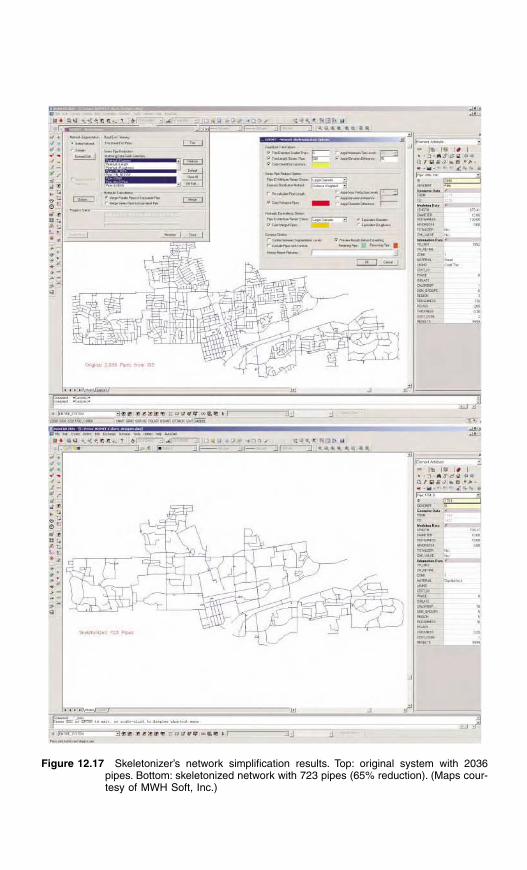
Figure 12.17 Skeletonizer’s network simplification results. Top: original system with 2036pipes. Bottom: skeletonized network with 723 pipes (65% reduction). (Maps cour-tesy of MWH Soft, Inc.)

Figure 13.10 AGSWMM toolbar and input form.
Figure 14.5 ArcFM screenshot showing water objects.

Figure 15.1 ArcGIS screenshot of mean pipeline ratings for the Metropolitan Sewerage District (MSD) of Buncombe County, NC.