i | P a g e

Document Control

Wanneroo Road / Joondalup Drive _______________________________

Main Roads Western Australia

Rapid Economic Analysis – Final Report

November 2017

ii | P a g e

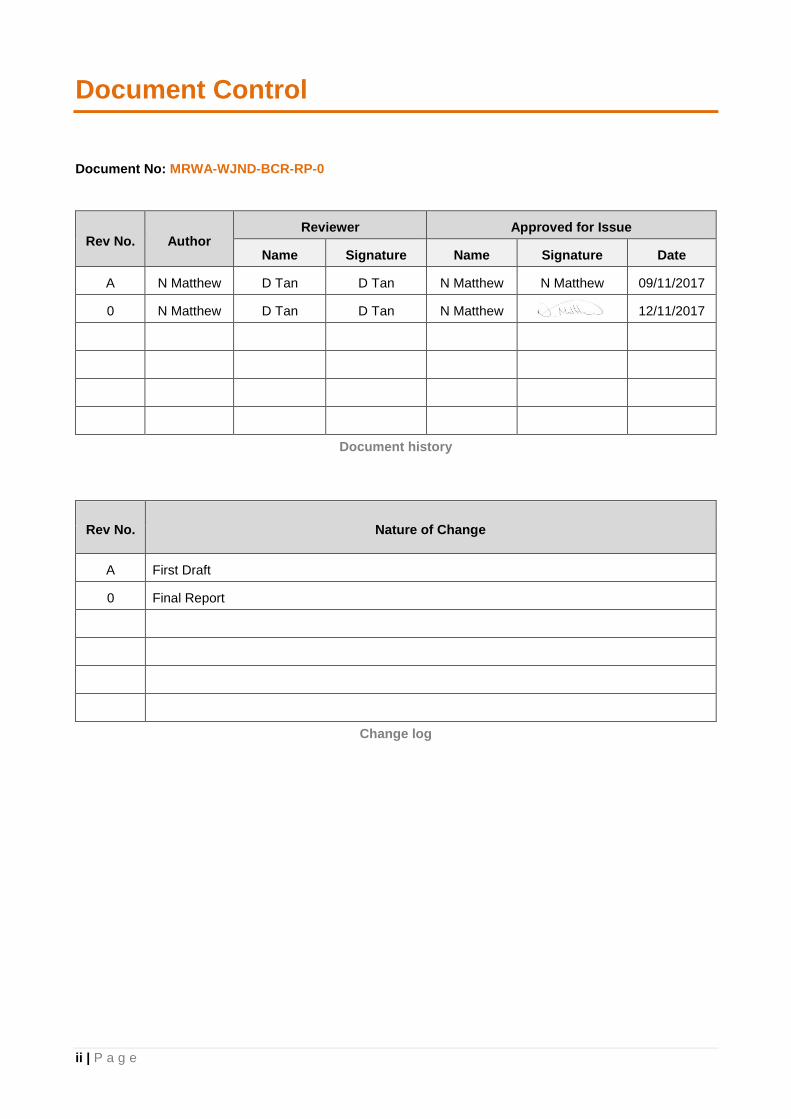
Document Control

Document No: MRWA-WJND-BCR-RP-0

Rev No. Author Reviewer Approved for Issue

Name Signature Name Signature Date

A N Matthew D Tan D Tan N Matthew N Matthew 09/11/2017

0 N Matthew D Tan D Tan N Matthew 12/11/2017

Document history

Rev No. Nature of Change

A First Draft

0 Final Report

Change log

iii | P a g e

Table of Contents

1 Introduction ................................................................................................................................................. 1

2 Investment Opportunity .............................................................................................................................. 2

3 Project Costs .............................................................................................................................................. 4

3.1 Capital Expenditure (CAPEX) ............................................................................................................ 4

3.2 Routine and Periodic Maintenance (OPEX) ...................................................................................... 4

3.3 Residual Values ................................................................................................................................. 4

3.4 Discounted Costs ............................................................................................................................... 5

3.5 Opening Date ..................................................................................................................................... 5

4 Economic Model Parameters ..................................................................................................................... 6

4.1 Methodology ...................................................................................................................................... 7

4.2 Peak Hour to Daily Conversion ......................................................................................................... 7

4.3 Annualisation ..................................................................................................................................... 8

4.4 Economic Project Life ........................................................................................................................ 8

4.5 Monetising VHT Differences .............................................................................................................. 9

4.6 Discount Rate .................................................................................................................................. 10

5 Results ...................................................................................................................................................... 11

5.1 Benefits ............................................................................................................................................ 11

5.2 Economic Indicators ........................................................................................................................ 12

5.2.1 BCR ............................................................................................................................................. 12

5.2.2 NPV .............................................................................................................................................. 12

5.2.3 IRR ............................................................................................................................................... 12

5.2.4 Payback Period ............................................................................................................................ 13

6 Sensitivity Analysis ................................................................................................................................... 13

6.1 Discount rate .................................................................................................................................... 13

7 Summary .................................................................................................................................................. 13

iv | P a g e

Index of Tables

Table 1 Capital expenditure ($M) ...................................................................................................................... 4

Table 2 Undiscounted OPEX ($M) .................................................................................................................... 4

Table 3 Discounted expenditure ($M) ............................................................................................................... 5

Table 4 Estimated values of urban travel time .................................................................................................. 9

Table 5 Estimated values of urban travel time ................................................................................................ 10

Table 6 VHT differences .................................................................................................................................. 11

Table 7 Undiscounted benefit summary ($M).................................................................................................. 11

Table 8 PVB summary ($M) ............................................................................................................................ 11

Table 9 BCR summary .................................................................................................................................... 12

Table 10 NPV summary ($M) .......................................................................................................................... 12

Table 11 IRR summary .................................................................................................................................... 12

Table 12 Payback period ................................................................................................................................. 13

Table 13 BCR results under varying discount rates ........................................................................................ 13

Index of Figures

Figure 1 Wanneroo Rd / Joondalup Dr aerial view ............................................................................................ 2

Figure 2 Wanneroo Rd / Joondalup Dr existing layout ...................................................................................... 3

Figure 3 Wanneroo Rd / Joondalup Dr proposed upgrades.............................................................................. 3

Figure 4 Weekday hourly traffic flow profile ....................................................................................................... 8

1 | P a g e

1 Introduction

Urbsol has been engaged by Main Roads Western Australia (MRWA) to assist with the economic analysis of

the proposed upgrade of the existing Wanneroo Road / Joondalup Drive intersection.

Traditionally, the benefits associated with transport infrastructure investment are assessed using 24-hour,

strategic four-step transport models. It is, however, well accepted that the approach adopted in these models

can be found wanting when applied to fine level network improvements, due generally to the necessarily

simplified treatment of detailed network operation and capacity in these models.

It is for this reason that use has been made of a first principles economic evaluation method focussed on the

economic benefits associated with improvements in vehicle hours of travel likely to be experienced by motorists

and as such, there are a number of other components that are omitted in this analysis, which include:

• Vehicle operating cost improvements

• Travel time reliability improvements

• Environmental cost reductions

• Crash savings

• Macroeconomic/secondary benefits

The general process involves the assessment, quantification and monetisation of vehicle hours of travel

improvements as a result of the Project.

The economic evaluation presented here has shown a viable project with a BCR of 1.52 at the 7% rate of

discount, a NPV of $24.59M and a payback period of 14 years. The internal rate of return is predicted to be

11%, which exceeds the social rate of discount.

2 | P a g e

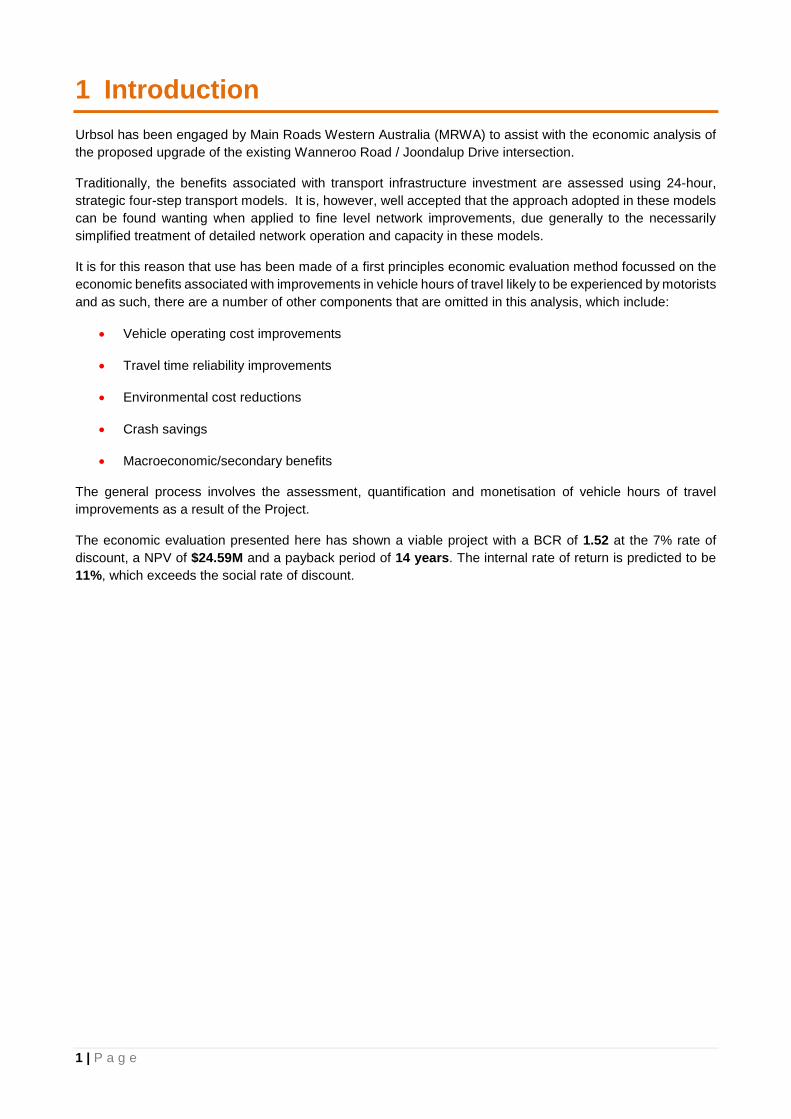
2 Investment Opportunity

The existing Wanneroo Road / Joondalup Drive intersection has been identified as a high priority location for

potential upgrade. The existing intersection is shown in Figure 1. Note that the north direction is to the bottom

left of the figure.

Figure 1 Wanneroo Rd / Joondalup Dr aerial view

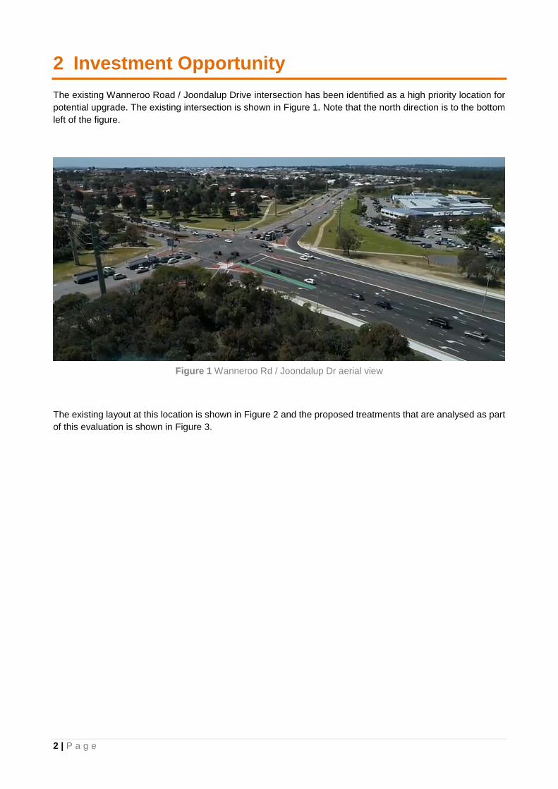
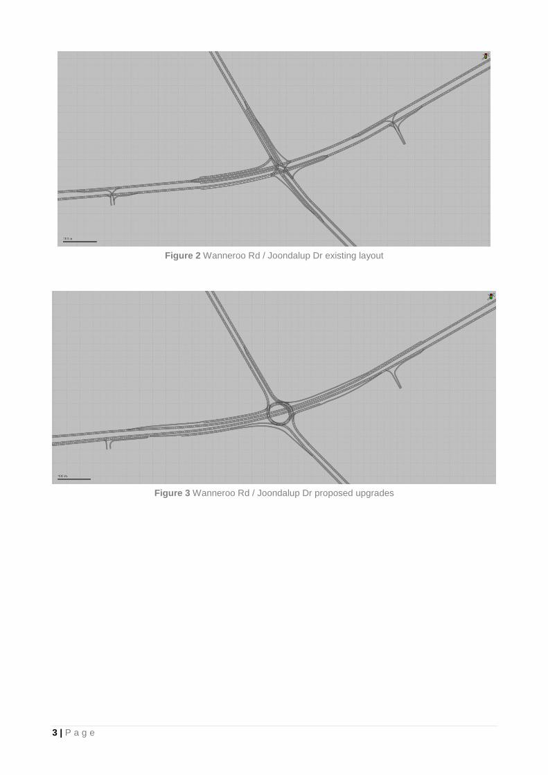
The existing layout at this location is shown in Figure 2 and the proposed treatments that are analysed as part

of this evaluation is shown in Figure 3.

3 | P a g e

Figure 2 Wanneroo Rd / Joondalup Dr existing layout

Figure 3 Wanneroo Rd / Joondalup Dr proposed upgrades

4 | P a g e

3 Project Costs

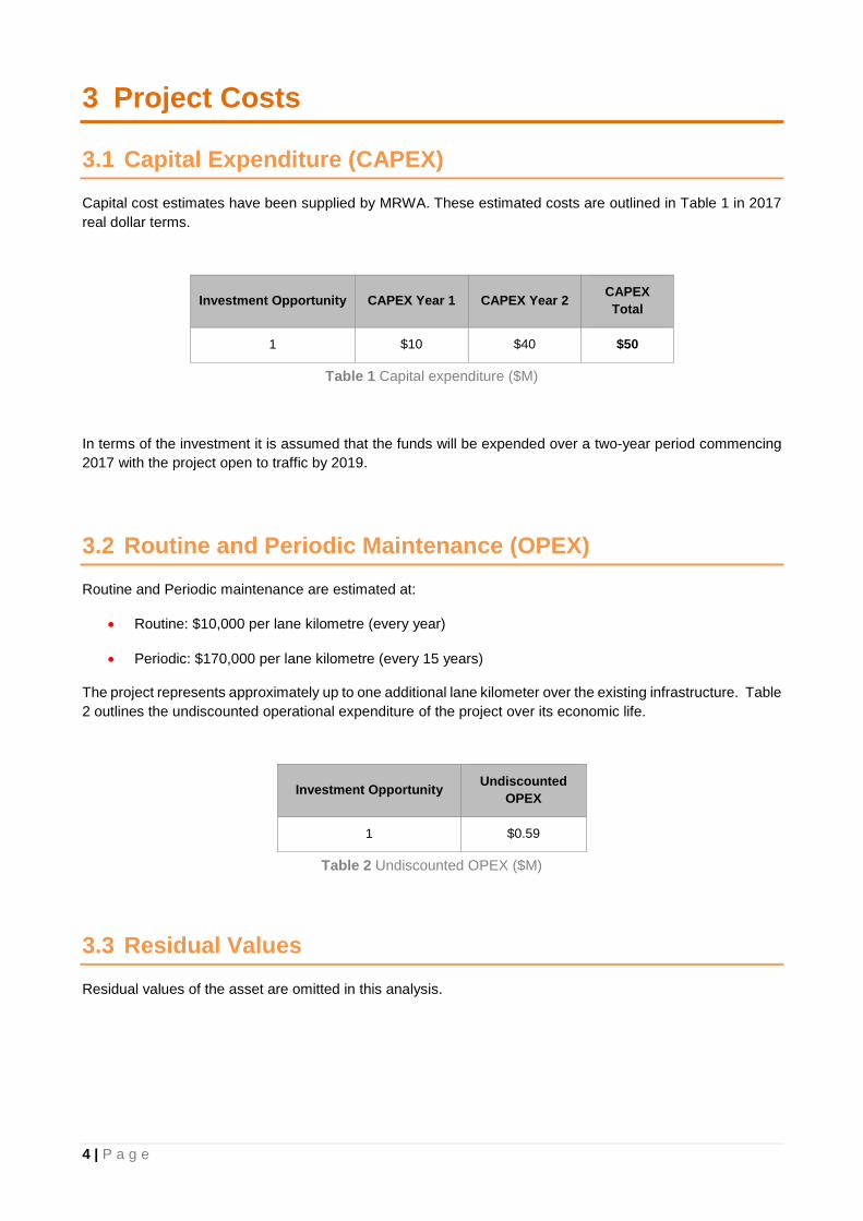
3.1 Capital Expenditure (CAPEX)

Capital cost estimates have been supplied by MRWA. These estimated costs are outlined in Table 1 in 2017

real dollar terms.

Investment Opportunity CAPEX Year 1 CAPEX Year 2 CAPEX

Total

1 $10 $40 $50

Table 1 Capital expenditure ($M)

In terms of the investment it is assumed that the funds will be expended over a two-year period commencing

2017 with the project open to traffic by 2019.

3.2 Routine and Periodic Maintenance (OPEX)

Routine and Periodic maintenance are estimated at:

• Routine: $10,000 per lane kilometre (every year)

• Periodic: $170,000 per lane kilometre (every 15 years)

The project represents approximately up to one additional lane kilometer over the existing infrastructure. Table

2 outlines the undiscounted operational expenditure of the project over its economic life.

Investment Opportunity Undiscounted

OPEX

1 $0.59

Table 2 Undiscounted OPEX ($M)

3.3 Residual Values

Residual values of the asset are omitted in this analysis.

5 | P a g e

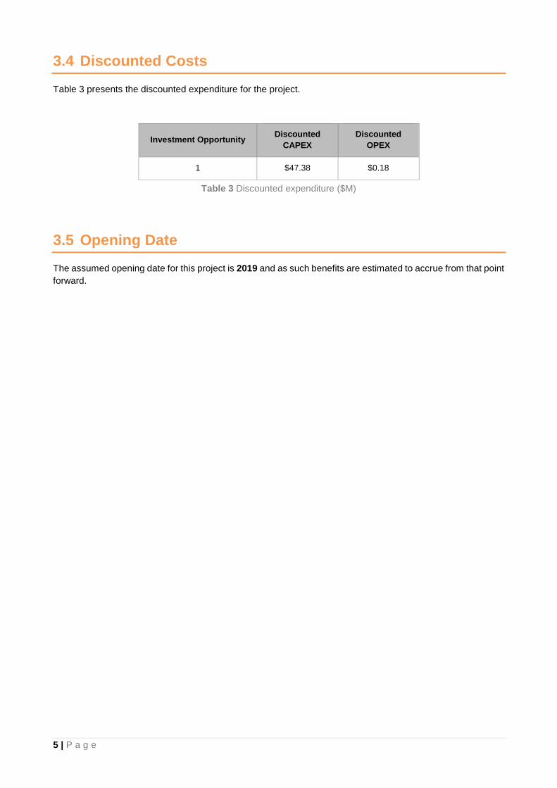
3.4 Discounted Costs

Table 3 presents the discounted expenditure for the project.

Investment Opportunity Discounted

CAPEX

Discounted

OPEX

1 $47.38 $0.18

Table 3 Discounted expenditure ($M)

3.5 Opening Date

The assumed opening date for this project is 2019 and as such benefits are estimated to accrue from that point

forward.

6 | P a g e

4 Economic Model Parameters

This economic assessment is based on the Australian Transport Assessment and Planning (ATAP), Guidelines

(2016) – PV2 – Road Transport.

Traditionally, the benefits associated with transport infrastructure investment are assessed using 24-hour,

strategic four-step transport models. It is, however, well accepted that the approach adopted in these models

can be found wanting when applied to fine level network improvements, due generally to the necessarily

simplified treatment of detailed network operation and capacity in these models.

It is for this reason that use has been made of a simulation based traffic model prepared for the study area

followed by first principles calculation of the benefit cost ratio applicable for the project.

Demand forecasts supplied for the economic analysis are derived from existing traffic survey data and ROM24

using standard state endorsed land use forecasts.

ROM24 is a 1160 zone, four-step strategic transport model covering the Perth metropolitan area built on the

CUBE/VOYAGER platform. It forms an important tool to assist both Main Roads and Local Governments in

maintaining a strong road network planning function.

These models are computer based mathematical systems that provide a means of estimating vehicle traffic

volumes on key links in the states metropolitan road network at various points in time. It consists of a series

of mathematical relationships that are derived from theory, surveys and observations to estimate travel

demand, mode choice and route choice characteristics of travellers.

The current base year networks available from ROM24 are:

• 2016

• 2021

• 2026

• 2031

• 2051

Each base year network consists of the previous base year network plus additional proposed projects.

ROM24 is an enhancement to MRWA’s strategic Regional Operations Model (ROM) which encompasses the

Perth metropolitan area and its surroundings. It is the only transport model in Perth capable of a true 24-hour,

time of day traffic assignment. The advantage of ROM24’s assignment methodology is that all-day (or time

period) link capacities are replaced with hourly capacities which are a measurable and intuitively

quantifiable. The sequential nature of the assignment means that residual congestion on saturated links can

linger on into the subsequent assignment hour. In this sense, ROM24 can mimic the phenomena of traffic flow

breakdown and recovery, which is currently beyond the capabilities of competing strategic models.

7 | P a g e

4.1 Methodology

As an economic evaluation with two forecast points, four scenarios are modelled for each investment

opportunity to determine the likely improvement in vehicle hours of travel as a result of the project:

1. Do-nothing network subjected to existing traffic demands

2. Do-nothing network subjected to 2031 traffic demands

3. Project network subjected to existing traffic demands

4. Project network subjected to 2031 traffic demands

The analysis of all options is performed using VISSIM.

The assessment is then based on the difference between the project and do-nothing scenario for each forecast

horizon with direct interpolation applied for intervening years between the model horizons.

As the analysis years only cover 2017 and 2031, there is also a need to extrapolate benefits out to a 30-year

assessment period. For the purposes of conservatism, benefits beyond 2031 are assumed to be flat rather

than following some form of escalation over time.

4.2 Peak Hour to Daily Conversion

The models developed only cover peak hour conditions and as such, there is a need to convert these peak

hour benefits to a daily level. The peak hour to daily conversion requires an understanding of typical weekday

hourly flow relative to the peak flows that occur in the morning and afternoon. For this purpose, daily profiles

were derived from the supplied 24-hour video survey.

These flow profiles are key in adjusting the expected vehicle hours of travel in both the do-nothing and project

cases to expand the peak hour models developed in capturing the likely time savings through a typical

weekday. As traffic flows during the hours around and between the peaks are less than the peak hours

themselves, a relative comparison is made between each hour in question. The peak hour flow and the relative

proportion is then multiplied by the difference in travel time between the do-nothing and project networks. For

this assessment, only hours where the off-peak period to peak period ratio is equal to or greater than 75% are

included in the benefit calculations.

The daily traffic flow profile is shown in Figure 4.

8 | P a g e

Figure 4 Weekday hourly traffic flow profile

In terms of the hours each day that have 75% or more of the peak flow (i.e. the hours during which benefits

are assumed to accrue):

• AM Hours: 2 hours

• PM Hours: 4 hours

4.3 Annualisation

The annualisation of the benefits is based on the assumption of 330 days per year to account for weekends,

public holidays and other abnormal traffic conditions.

4.4 Economic Project Life

Infrastructure projects are typically assessed over a project lifecycle of 30 years and as such economic metrics

are based on an assessment out to 2048. For the purposes of conservatism, undiscounted benefits beyond

2031 are assumed to be flat rather than follow some form of escalation over time.

9 | P a g e

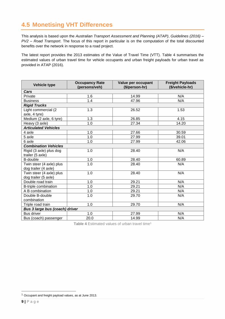
4.5 Monetising VHT Differences

This analysis is based upon the Australian Transport Assessment and Planning (ATAP), Guidelines (2016) –

PV2 – Road Transport. The focus of this report in particular is on the computation of the total discounted

benefits over the network in response to a road project.

The latest report provides the 2013 estimates of the Value of Travel Time (VTT). Table 4 summarises the

estimated values of urban travel time for vehicle occupants and urban freight payloads for urban travel as

provided in ATAP (2016).

Vehicle type Occupancy Rate

(persons/veh) Value per occupant

($/person-hr) Freight Payloads

($/vehicle-hr)

Cars

Private 1.6 14.99 N/A

Business 1.4 47.96 N/A

Rigid Trucks

Light commercial (2 axle, 4 tyre)

1.3 26.52 1.53

Medium (2 axle, 6 tyre) 1.3 26.85 4.15

Heavy (3 axle) 1.0 27.34 14.20

Articulated Vehicles

4 axle 1.0 27.66 30.59

5 axle 1.0 27.99 39.01

6 axle 1.0 27.99 42.06

Combination Vehicles

Rigid (3 axle) plus dog trailer (5 axle)

1.0 28.40 N/A

B-double 1.0 28.40 60.89

Twin steer (4 axle) plus dog trailer (4 axle)

1.0 28.40 N/A

Twin steer (4 axle) plus dog trailer (5 axle)

1.0 28.40 N/A

Double road train 1.0 29.21 N/A

B-triple combination 1.0 29.21 N/A

A B combination 1.0 29.21 N/A

Double B-double combination

1.0 29.70 N/A

Triple road train 1.0 29.70 N/A

Bus 3 large bus (coach) driver

Bus driver 1.0 27.99 N/A

Bus (coach) passenger 20.0 14.99 N/A

Table 4 Estimated values of urban travel time1

1 Occupant and freight payload values, as at June 2013.

10 | P a g e

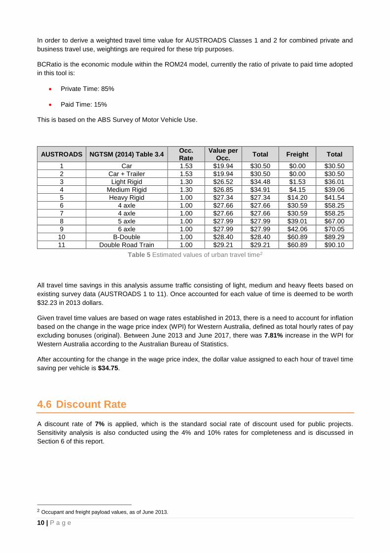
In order to derive a weighted travel time value for AUSTROADS Classes 1 and 2 for combined private and

business travel use, weightings are required for these trip purposes.

BCRatio is the economic module within the ROM24 model, currently the ratio of private to paid time adopted

in this tool is:

• Private Time: 85%

• Paid Time: 15%

This is based on the ABS Survey of Motor Vehicle Use.

AUSTROADS NGTSM (2014) Table 3.4 Occ. Rate

Value per Occ.

Total Freight Total

1 Car 1.53 $19.94 $30.50 $0.00 $30.50

2 Car + Trailer 1.53 $19.94 $30.50 $0.00 $30.50

3 Light Rigid 1.30 $26.52 $34.48 $1.53 $36.01

4 Medium Rigid 1.30 $26.85 $34.91 $4.15 $39.06

5 Heavy Rigid 1.00 $27.34 $27.34 $14.20 $41.54

6 4 axle 1.00 $27.66 $27.66 $30.59 $58.25

7 4 axle 1.00 $27.66 $27.66 $30.59 $58.25

8 5 axle 1.00 $27.99 $27.99 $39.01 $67.00

9 6 axle 1.00 $27.99 $27.99 $42.06 $70.05

10 B-Double 1.00 $28.40 $28.40 $60.89 $89.29

11 Double Road Train 1.00 $29.21 $29.21 $60.89 $90.10

Table 5 Estimated values of urban travel time2

All travel time savings in this analysis assume traffic consisting of light, medium and heavy fleets based on

existing survey data (AUSTROADS 1 to 11). Once accounted for each value of time is deemed to be worth

$32.23 in 2013 dollars.

Given travel time values are based on wage rates established in 2013, there is a need to account for inflation

based on the change in the wage price index (WPI) for Western Australia, defined as total hourly rates of pay

excluding bonuses (original). Between June 2013 and June 2017, there was 7.81% increase in the WPI for

Western Australia according to the Australian Bureau of Statistics.

After accounting for the change in the wage price index, the dollar value assigned to each hour of travel time

saving per vehicle is $34.75.

4.6 Discount Rate

A discount rate of 7% is applied, which is the standard social rate of discount used for public projects.

Sensitivity analysis is also conducted using the 4% and 10% rates for completeness and is discussed in

Section 6 of this report.

2 Occupant and freight payload values, as of June 2013.

11 | P a g e

5 Results

5.1 Benefits

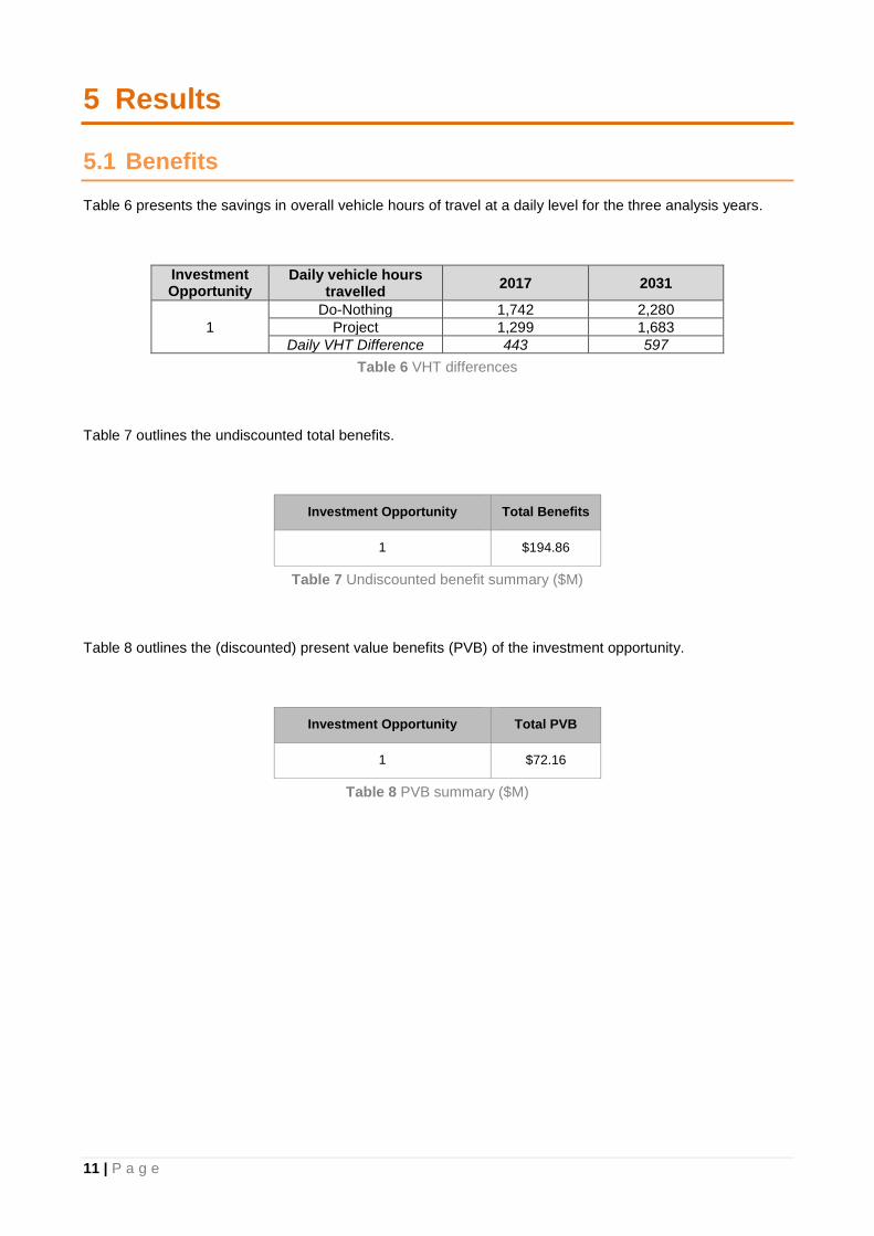
Table 6 presents the savings in overall vehicle hours of travel at a daily level for the three analysis years.

Investment Opportunity

Daily vehicle hours travelled

2017 2031

1

Do-Nothing 1,742 2,280

Project 1,299 1,683

Daily VHT Difference 443 597

Table 6 VHT differences

Table 7 outlines the undiscounted total benefits.

Investment Opportunity Total Benefits

1 $194.86

Table 7 Undiscounted benefit summary ($M)

Table 8 outlines the (discounted) present value benefits (PVB) of the investment opportunity.

Investment Opportunity Total PVB

1 $72.16

Table 8 PVB summary ($M)

12 | P a g e

5.2 Economic Indicators

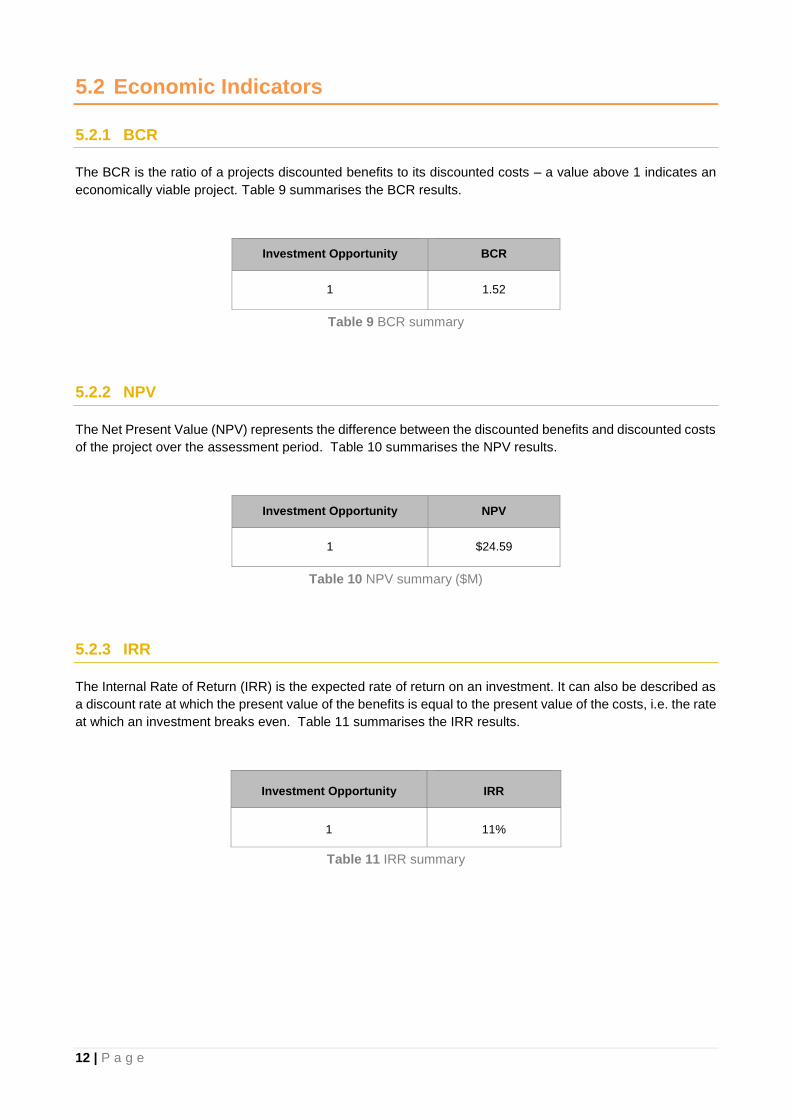
5.2.1 BCR

The BCR is the ratio of a projects discounted benefits to its discounted costs – a value above 1 indicates an

economically viable project. Table 9 summarises the BCR results.

Investment Opportunity BCR

1 1.52

Table 9 BCR summary

5.2.2 NPV

The Net Present Value (NPV) represents the difference between the discounted benefits and discounted costs

of the project over the assessment period. Table 10 summarises the NPV results.

Investment Opportunity NPV

1 $24.59

Table 10 NPV summary ($M)

5.2.3 IRR

The Internal Rate of Return (IRR) is the expected rate of return on an investment. It can also be described as

a discount rate at which the present value of the benefits is equal to the present value of the costs, i.e. the rate

at which an investment breaks even. Table 11 summarises the IRR results.

Investment Opportunity IRR

1 11%

Table 11 IRR summary

13 | P a g e

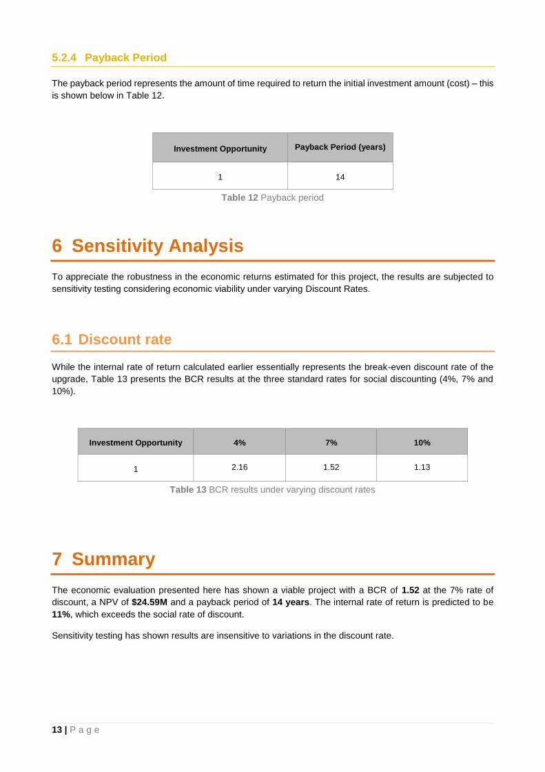
5.2.4 Payback Period

The payback period represents the amount of time required to return the initial investment amount (cost) – this

is shown below in Table 12.

Investment Opportunity Payback Period (years)

1 14

Table 12 Payback period

6 Sensitivity Analysis

To appreciate the robustness in the economic returns estimated for this project, the results are subjected to

sensitivity testing considering economic viability under varying Discount Rates.

6.1 Discount rate

While the internal rate of return calculated earlier essentially represents the break-even discount rate of the

upgrade, Table 13 presents the BCR results at the three standard rates for social discounting (4%, 7% and

10%).

Investment Opportunity 4% 7% 10%

1 2.16 1.52 1.13

Table 13 BCR results under varying discount rates

7 Summary

The economic evaluation presented here has shown a viable project with a BCR of 1.52 at the 7% rate of

discount, a NPV of $24.59M and a payback period of 14 years. The internal rate of return is predicted to be

11%, which exceeds the social rate of discount.

Sensitivity testing has shown results are insensitive to variations in the discount rate.

14 | P a g e

Disclaimer and Copyright

This document and any attached files (“material”) are the property of Urban Modelling Solutions (Urbsol). Any

reproduction of the concepts, ideas, or content of the material is strictly prohibited without the prior consent of

the owner/author.

Urbsol accepts no liability and implies no warranty or other assurance for reliance on the content of the

material. Although all best efforts have been made Urbsol in no way guarantees the accuracy, completeness,

timelessness or fitness for any particular purpose of the material. Any parties relying on this material do so at

their own risk.

Data used in this work is largely provided by third parties and Urbsol can in no way attest for the accuracy or

otherwise of this.

To the full extent permissible by law, Urbsol disclaims all responsibility and liability (including for negligence)

for any damages or losses (including, without limitation, financial loss, damages for loss in business projects,

loss of profits or savings or other consequential losses) arising in contract, tort or otherwise from any action or

decision taken as a result of the use or inability to use the material. Information in the material is made available

without warranty or responsibility on the part of Urbsol.

This material is not designed as providing a detailed action plan nor is it to be interpreted as proposing absolute

solutions to likely traffic issues. Traffic modelling and analysis can provide an indication of likely outcomes but

is not designed to replace professional judgment. This material is designed to aid and complement decision

making.