wär- ;/6 · supplying the experimental data used in section 6.3, Alex Kilpatrick of IVISC/NASTRAN...

Improvement of Structural Dynamic Models

via System Identification

bvS Peter A. Stiles

S Thesis submitted to the Faculty of theVirginia Polytechnic Institute and State University

in partial fulfillment of the requirements for the degree of

Master of Science

in_

Mechanical Engineering

APPROVED:

A· . ; M,/7 _

r. Jo 1 B. Kosmatka, Chairman Dr. Robert H. Fries

7 · „AAAA\\‘~

•.;§( \/« wär- ;/6ls.Dr.Raphael T. aftka Dr. Charles F.ReinholtzDecember

1988

Blacksburg, VirginiaA

Improvement of Structural Dynamic Models

_viaSystem Identification

bvPeter A. StilesV·

Dr. John B. Kosmatka, ChairmanI

Mechanical Engineering

(ABSTRACT)

Proper mathematical models of structures are beneficial for designers and

analysts. The accuracy of the results is essential. Therefore, verification and/or

correction of the models is vital. This can be done by utilizing experimental results

or other analytical solutions. There are different methods of generating the accurate

mathematical models. These methods range from completely analytically derived

models, completely experimentally derived models, to a combination of the two.

These model generation procedures are called System Identification. Today a

popular method is to create an analytical model as accurately as possible and then

improve this model using experimental results.

This thesis provides a review of System Identification methods as applied to

vibrating structures. One simple method and three more complex methods, chosen

from current engineering literature, are implemented on the computer. These

methods offer the capability to correct a discrete (for example, finite element based)

model through the use of experimental measurements. The validity of the methods

is checked on a two degree of freedom problem, an eight degree of freedom example

frequently used in the literature, and with experimentally derived vibration results of

a free—free beam.

· I

I S II .II

Acknowledgements

I would like to thanks Drs. J. Kosmatka, R. Fries, R. Haftka, and C. Reinholtz for

serving on my committee. Special thanks go to Dr. Kosmatka for providing Insight,

help, and guidance where needed. His methods of advising were well appreciated

and respected. Additionally, I would like to thank; Ron Rorrer and Dr. A. VI/icks for

supplying the experimental data used in section 6.3, Alex Kilpatrick of IVISC/NASTRAN

for helping with DMAP problems, all those who helped solve SCRIPT and SAS

problems, and NSVVC/DL for supplying research funds for my first year.

l\/ly family and friends offered support, love, strength, and advice. They all helped

keep me on course during my time in Virginia.

Thanks to all the people in Blacksburg who helped make this experience a

beneficial one. The breaks from academia including; camping, volleyball, hiking,

fishing, happy hours and lengthy discussions, were beneficial.

Thanks go to all the unmentioned people in my life who have inspired me to

learn, as well as to pursue this degree. Final appreciation goes to the original VI/Pl

Plan.

. Acknowledgements iii

Table of Contents

INTRODUCTION AND REVIEW OF PRESENT RESEARCH .......................... 1

1.1 Introduction ........................................................ 1

1.2 Review of Literature ..................................................4

1.2.1 Verification method ............................................... 8

1.2.2 Modification method ............................................. 11

1.2.3 Direct Identification Method ........................................ 16

1.2.4 Related Topics .................................................. 17

1.3 Organization of Thesis ............................................... 19

METHOD BASED ON EIGENVALUE SENSITIVITY ............................... 21

2.1 Introduction ....................................................... 21

2.2 Development ...................................................... 22

2.3 Implementation .................................................... 25

METHOD THAT UTILIZES ORTHOGONALITY EQUATIONS ........................ 29

3.1 Introduction ....................................................... 29

3.2 Development ...................................................... 31

l Table of Contents iv

li

3.3 Implementation .................................................... 36

METHOD BASED ON CONNECTIVITY CONSTRAINT ............................. 39

4.1 Introduction ....................................................... 39

4.2 Development ...................................................... 40

4.3 Implementation .................................................... 48

METHOD BASED ON RESIDUAL FORCE VECTOR .............................. 51

5.1 Introduction ....................................................... 51

5.2 Development ...................................................... 52

5.3 Implementation .................................................... 57

NUMERICAL RESULTS ................................................... 60

6.1 Verification Studies - 2 DOF model ...................................... 60

6.2 Modification Studies using an 8 DOF Model ............................... 73

6.3 Application of Methods with data for a free-free beam ....................... 82

CONCLUSIONS AND RECOMMENDATIONS .................................. 105

7.1 Conclusions ...................................................... 105

7.2 Recommendations ................................................. 107

REFERENCES ......................................................... 110

Modeling and Solution Sequences from MSC/NASTRAN ........................ 115

A.1 Solution Sequence for Sensitivity Based Method .......................... 116

A.2 Solution Sequence for Orthogonality Based Method ....................... 126

A.3 Solution Sequence for Connectivity Constraint Based Method _................129A.4

Solution Sequence for Residual Force Based Method ...................... 136 jIl

Table of Contents v II

l

II

Vita ................................................................ 147 II

I

II

I

Table of Contents vi II

I

List of Illustrations

Figure 1. 2 DOF SPRING MASS SYSTEM USED FOR EXAMPLE 1 ...........62

Figure 2. 8 DOF TEST PROBLEM, DEVELOPED BY KABE, USED FOR SECONDEXAMPLE ..............................................74

Figure 3. ERROR IN PREDICTED FREQUENCY WITH SENSITIVITY METHOD FOR8 DOF EXAMPLE .........................................77

Figure 4. ERROR IN PREDICTED FREOUENCY WITH ORTHOGONALITY METHODFOR 8 DOF EXAMPLE .....................................78

Figure 5. ERROR IN PREDICTED FREOUENCY WITH CONNECTIVITY METHODFOR 8 DOF EXAMPLE .....................................79

Figure 6. ERROR IN PREDICTED FREOUENCY WITH RES. FORCE METHOD FOR8 DOF EXAMPLE .........................................81

Figure 7. ILLUSTRATION OF BEAM USED FOR EXAMPLE 3 AND THE FINITEELEMENT MODEL ........................................83

Figure 8. ERROR IN FREOUENCY PREDICTION FOR BEAM USING SENSITIVITYMETHOD ...............................................85

Figure 9. CONVERGENCE OF FREOUENCIES WHEN USING SENSITIVITY METHOD 86

Figure 10. ERROR IN FREOUENCY PREDICTION FOR BEAM USINGORTHOGONALITY METHOD ................................88

Figure 11. EXTRANEOUS MODE INTRODUCED BY ORTHOGONALITY METHOD . . 89

Figure 12. ERROR IN FREOUENCY PREDICTION FOR BEAM USINGCONNECTIVITY METHOD ..................................90

Figure 13. FREOUENCY PREDICTION FOR THE CONNECTIVITY METHOD ......91

Figure 14. ERROR IN FREOUENCY PREDICTION FOR BEAM USING RES. FORCEMETHOD ...............................................93

List of Illustrations vii

Figure 15. FIRST EXPERIMENTAL MODE SHAPE OF THE FREE·FREE BEAM ....94

Figure 16. SECOND EXPERIMENTAL MODE SHAPE OF THE FREE·FREE BEAM . . 95

Figure 17. THIRD EXPERIMENTAL MODE SHAPE OF THE FREE-FREE BEAM ....96

Figure 18. FOURTH EXPERIMENTAL MODE SHAPE OF THE FREE-FREE BEAM . . 97

Figure 19. FIFTH EXPERIMENTAL MODE SHAPE OF THE FREE-FREE BEAM ....98

Figure 20. SIXTH EXPERIMENTAL MODE SHAPE OF THE FREE·FREE BEAM ....99

List ¤r Illustrations viii

II

List of Tables

Table 1. TABLE OF VARIABLE VALUES FOR TESTS 1a - 1f ................63

Table 2. INITIAL PARAMETERS AND RESULTS OF TEST 1a ...............65

Table 3. INITIAL PARAMETERS AND RESULTS OF TEST 1b ...............66

Table 4. INITIAL PARAMETERS AND RESULTS OF TEST 1c ...............67

Table 5. INITIAL PARAMETERS AND RESULTS OF TEST 1d ...............68

Table 6. INITIAL PARAMETERS AND RESULTS OF TEST 1e ...............70

Table 7. INITIAL PARAMETERS AND RESULTS OF TEST1f72

Table 8. RELATl\/E CHANGES TO MATRICES, # OF DIAGONAL TERMSCHANGED .............................................101

Table 9. RELATIVE CHANGES TO MATRICES, # OF OFF-DIAGONAL TERMSCHANGED .............................................102

Table 10. CPU TIME REOUIRED FOR THE FOUR METHODS FOR FREE-FREEBEAM Iminzsec) .........................................104

l Last bl Tables ixII

Nomenclature

a Multiplier of element stiffness matrix

[A] = 4 [I)/l.][<l>.][#.]b Multiplier of element mass matrix

[B] = [M.] [A4] Eu.] + [M.] [du] [Au] — [K.] [A4][B] [B] partitioned into a column

[D] Matrix used in connectivity method, see eq (4.26)

DOF Degree of Freedom

f Frequency,second

[HJ.) = — [E], rom[I] Identity Matrix

Matrix used to update stiffness matrixwhere li, =1 if Kan #1 or

else I, = 0 er Kan = 0 E

[k] Element Stiffness Matrix

[K] Global Stiffness Matrix

[AK] Change in stiffness matrix

= [K.] — [K.]I Number of Design Variables

m Number of Experimental Frequencies

Nomenclature X

[ma] = [.]‘[lVl„] [<l>.][m] Element Mass Matrix

[M] Global Mass Matrix

[AM] Change in mass matrix

= [M.] — [M.,]n Number of Analytical DOF

[N] = [l\/1.]*/2r Number of deficient elements in model

[Q] Matrix obtained in residual force method, see eq (5.14)

[R] Residual Force Matrix

= — [l<.][d>.] + [M.][„][u.][X] Column Vector of Design Variables

[Z] Column Vector of Unknown matrix multipliers, a and b

Greek Letters

[lx] Matrix used in connectivity method, see eq (4.22)

[ß] Matrix used in connectivity method, see eq (4.23)

6 Error function

ÖX, Change in jth design variable

[A] Matrix used to update mass matrix

[y] Matrix used to update stiffness matrix

A Lagrangian multiplier

[A] Matrix of Lagrangian multipliers

[Al] ith row of [A]

with all other rows set to

zeroNomenclature xil

i

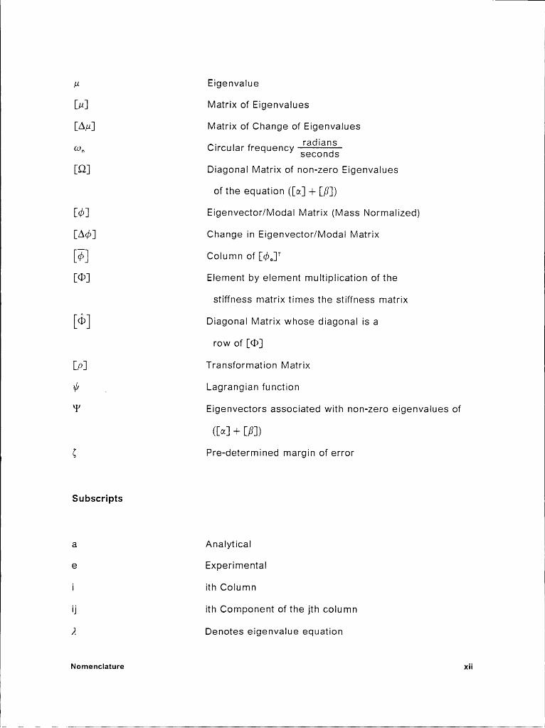
ii Eigenvalue

[0] Matrix of Eigenvalues

[Au] Matrix of Change of Eigenvalues

0;,, Circular frequencyseconds

[Q] Diagonal Matrix of non-zero Eigenvalues

of the equation ([a] —l— [,6])[gb] Eigenvector/Modal Matrix (Mass Normalized)

[Agb] Change in Eigenvector/Modal Matrix

Column of [gb,,]’

[<D] Element by element multiplication of the

stiffness matrix times the stiffness matrixDiagonal Matrix whose diagonal is a

row of [CD]

[p] Transformation Matrix

i/1 Lagrangian function‘P

Eigenvectors associated with non-zero eigenvalues of

(Dx] + [,6])§ Pre-determined margin of error

Subscripts

a Analytical

e Experimental

i ith Columnij ith Component of the jth column

Ä Denotes eigenvalue equation

tNomenclature xiil

ii

O Denotes orthogonality equation

S Denotes symmetry condition

u Updated

, Partial Derivative

Superscripts

T Transpose

Nomenclature xiiii

Chapter I 1

INTRODUCTION AND REVIEW OF PRESENT

1.1 Introduction

Analytical methods of problem solving have become more prominent with

advances in technology. Computer modelling techniques, such as finite element

methods, which predict the response of structures to loads, have become accepted.

However, these approaches do not always yield accurate results, as the formulations

are based on assumptions, that may not be completely valid for the problem being

modelled. In addition to these errors, modelling errors can exist which are

dependent on the model refinement, human errors, and solution techniques for large

problems. There is an increasing need to verify the models of structures and to learn

, iuraooucriou Auo Review oe masseur iaessmacn 1

how to compensate for the inaccuracies that exist. By doing this, discrete models

will be able to predict the response of structures more accurately.

When properly used, finite element methods have been shown to properly model

structures (Zienkiewicz, 1967).l Computer modelling techniques are invaluable in the

aerospace industry. The space shuttle, satellites, and airplanes have all benefitted

from the use of these techniques. Many modern structures are very complicated.

They can be comprised of complex shapes, non-linear boundary conditions, stress

concentrations, composite and non—Ilnear material properties. Computer modelling

offers an excellent opportunity to analyze a complex design, and to study the effect

of design changes. Hence, it is usually both time and cost effective to utilize

computer models.

lf the developed analysis method properly represents the problem being

analyzed, then an infinite number of elements using infinite precision will yield the

exact results. However, a model with a large number of elements costs more than

one with fewer elements. To save money and time, computationally smaller models

are desired.

Alternatively, if the developed computer method does not represent the problem

of interest, then "System ldentiflcation" may be able to generate a model which does.

System Identification is the process by which a system is generated by examinlng the

response as a function of the input. Modelling problems arise when the material

properties are not known exactly, or when previously mentioned complex problems

exist. lt is also difficult to measure the stiffness of a sub region of a structure, as the

structure is continuous and it is awkward to measure the stiffness of a section

l Authors names and dates in parenthesis indicate where to find the reference in the alphabetizedreference list at the end of this thesis. .

INTRODUCTION AND REVIEW OF PRESENT RESEARCH 2

II

directly. A goa! of System Identification is to keep the cost of analysis low while

achieving accurate results.

ln the field of vibrations, a popular System Identification method is to combine

an analytica! model with experimental data to generate a more accurate theoretical

model, ln dynamics, a discrete analytica! model yields eigenvalues and

eigenvectors. Eigenvalues correspond to the circular frequency squared, wß . The

eigenvectors correspond to the discretized mode shape vectors. For normal modes,

these modal vectors are orthogonal to each other with respect to the mass matrix and

measure relative deflection of the structure if it where vibrating only at the

corresponding frequency. Using this procedure, the experimental data is used as a

guide to change the analytica! model.

Experimental data offers the ability to verify at least some results of a model.

This data can be in the form of strain, deflection, natural frequencies, etc,. By utilizing

experimental results, computer models can be verified and/or fine tuned to more

accurately predict the response of a structure. A variety of methods exist and offer

different benefits. Some attempt to extract different parameter values, while others

have varying constraints which must be met while altering the model.

This thesis will review many of the current System Identification methods. Four

methods are implemented on a VAX 11/780 within l\/ISC/NASTRAN Version 65b

(MacneaI—Schwend!er,1984). They are methods based upon; (1) the sensitivity of the

frequencies with respect to the design variables (classical approach), (2) requiring

the experimental modes to be orthogonal to the analytica! system matrices, (Berman

and Nagy, 1983), (3) requiring the connectivity ofthe updated matrices to be the same

as the original matrices (Kabe, 1985), and (4) Iocating errors in the analytica! model

using a residual force vector (Chen and V!/ang, 1988). A simple two DOF spring mass

system is used to illustrate the capabilities of each method. The second problem,

INTRODUCTION AND REVIEW oI= PRESENT RESEARCH 3

l

developed by A. M. Kabe (1985), is an eight DOF, undamped, free Vibration, modelconsisting of lumped masses and springs. All methods will be used to identify the

modes of a free-free beam with experimentally derived mode shapes and natural

frequencies. The experimental data contains the translational displacementsobtained at 19 points along a 36 in. steel beam (Rorrer et al., 1989). Finally,

conclusions and recommendations will be presented covering the basic capabilities

and deficiencies of the four methods.

1.2 Review of Literature

Man has had a desire to study and analyze his surroundings ever since the

beginning of time. Many times this desire begins with an theoretical model that

needs to be modified or corrected, depending on experimental results. An accurate

understanding of Halley’s comet was developed utilizing System Identification

techniques (as detailed by Lancaster—Brown (1985)). First, an understanding of

Newtonian mechanics provided an a priori model of Halley’s comet. The previous

sightings of the comet were then used to alter the existing model. Halley applied

what was known and utilized experimental data to obtain a more accurate

understanding of Halley’s comet. He was able to predict the return of his comet fifty

years before it reappeared in 1758.

System Identification is used in many different fields. It is a means by which a

set of equations is generated by examining the response of the system to the input,

or given a response and an input, determine the system. A general interpretation of

System Identification implies that a system of equations is developed or identified

iN‘rRo¤uc‘noN AN¤ REVIEW OF PRESENT RESEARCH 4

which properly represents the system of interest. Often this set of equations or

relationships developed needs to be utilized and interpreted as a system. However,

it would be beneficial to be able to determine actual physical and geometric

properties of a system.

The identification of parameters of a system is called "parameter estimation.”

Often there is not enough data available to verify and determine the parameters of a

system. ln such cases, it can be very difficult, if not impossible, to generate a unique

system. For example, with a set of linear equations in order to uniquely identify a

system, there must be the same number of independent unknowns as there are

independent identifiable equations.

Depending on how a system is sub-divided and what types of assumptions are

made, a system can be over—constrained or under-constrained. If every component

of the mass and stiffness matrices are taken as unknowns, usually the number of

unknowns are greater than the number of equations. ln vibration analysis, the

number of equations is related to the quantity of experimental modal data in the form

of the mode shapes and natural frequencies. lf a parameter used for generating theA

matrices (i.e. Youngs modulus, density, thickness, etc.) is used as a variable which

does not vary from element to element in the finite element model, then often the

number of equations may be greater than the number of unknowns. These

differences and how they are interpreted define the basis of different sub-classes of

System Identification methods.

Many advances in methods for System Identification came with more accessible

computer power. These methods rely on computationally intensive analytical

techniques to create large models. A review of System Identification concepts as

applied to a variety of fields can be found in "System Identification Techniques: A

tutorial Review" (Jain and Dobeck,1979). There have been many articles in


engineering literature which review a certain class of methods, or reference related

articles; (Berman, 1979a), (Pakstys, 1982), (I—leylan and Sas, 1986), (Ibrahim and

Saafan, 1986), (Caesar, 1986). The review in this thesis gives an in depth overviewof many types of methods. A review of concepts and classifications of systemidentification as applied to vibrating structures is presented by Berman (1975).

Berman divides System Identification into three groups: verification, modification and

direct identification.

Verification relies on the analyst and deals with varying the individual

parameters, or design variables, in an analytical model until a correct model is

generated. This can be done by an individual utilizing an iterative intuitive procedure

or through the use of a procedure which systematically varies the parameters.

l\/Iodification deals with altering the components of the global mass and stiffness

matrices. Different procedures of matrix modification and utilization of constraint

equations distinguish the many different methods which fall under the modification

label. Direct identification deals with generating an analytical model directly from

experimental data. This method, unlike the other two, does not rely on initial

estimates for parameters of the model.

The mathematical model which results from applying System Identification

techniques can be classified as either a ’correct’ or ’physically correct' model. A

correct model is one that predicts the response of the structure, but which may not

yield realistic physical properties, i.e., new load paths or unreasonable values may

have been introduced. In order for a model to be physically correct, it should yield

the correct connectivity relationships, geometric properties, and material properties.

This enables one to gain a better understanding of the modelling errors and other

lnherent problems in the original analytical model, as well as making the resulting

model more understandable.

INTRODUCTION AND REVIEW oI= PRESENT RESEARCH 6III

, I

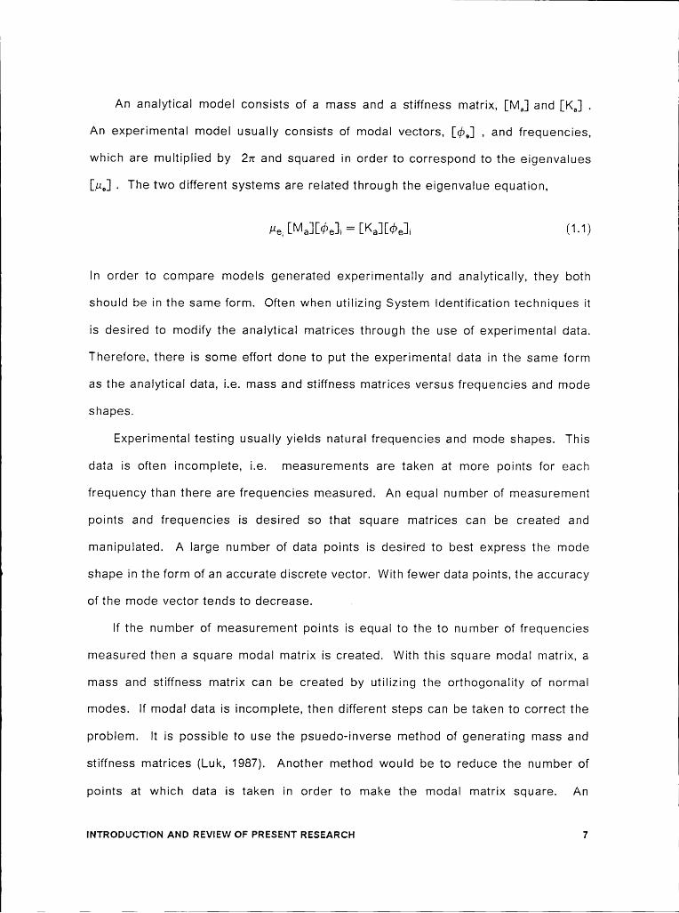
IAn analytical model consists of a mass and a stiffness matrix, [l\/I6] and [K6] . I

An experimental model usually consists of modal vectors, [$6] , and frequencies,

which are multiplied by 21z and squared in order to correspond to the eigenvalues

[II6] . The two different systems are related through the eigenvalue equation,

(1-1)

ln order to compare models generated experimentally and analytically, they both

should be in the same form. Often when utilizing System Identification techniques it

is desired to modify the analytical matrices through the use of experimental data.

Therefore, there is some effort done to put the experimental data in the same form

as the analytical data, i.e. mass and stiffness matrices versus frequencies and mode

shapes.

Experimental testing usually yields natural frequencies and mode shapes. This

data is often incomplete, i.e. measurements are taken at more points for each

frequency than there are frequencies measured. An equal number of measurement

points and frequencies is desired so that square matrices can be created and

manipulated. A large number of data points is desired to best express the mode

shape in the form of an accurate discrete vector. With fewer data points, the accuracy

of the mode vector tends to decrease. .

lf the number of measurement points is equal to the to number of frequencies

measured then a square modal matrix is created. With this square modal matrix, a

mass and stiffness matrix can be created by utilizing the orthogonality of normal

modes. lf modal data is incomplete, then different steps can be taken to correct the

problem. lt is possible to use the psuedo-inverse method of generating mass and

stiffness matrices (Luk, 1987). Another method would be to reduce the number of

points at which data is taken in order to make the modal matrix square.

AnINTRODUCTIONAND REVIEW oI= PRESENT RESEARCH 7 ÄI

alternative method is to add Iinearly independent mode shape vectors to the matrixwhile requiring that their associated frequencies are large. Another alternative would

be to synthesize the flexibility matrix instead of the stiffness matrix and compare theflexibility matrices.

In an analytica! analysis it is possible to generate eigenvalues and eigenvectors.This is similar to the form the experimental data is in, hence it is easy to compare the

modal data, instead of the matrices. This is good for comparison of results, but does

not enable one to directly modify the system matrices. ln order to keep the matrices

physically correct, one usually wants to make minimum changes to the system

matrices. l\/linimizing the percent changes to the components of the matrices is

difficult to do if the mode shape vectors are modified and the system matrices are

determined through matrix manipulations.

Problems can result when trying to compare an analytica! mode! and an

experimental model, or experimental results. Analytical models tend to have data

taken at more points than an experimental model would. Therefore, the analytica!

models are of greater dimension. In order to compare matrices of the same size, the

analytica! system matrices can be reduced to be ofthe same size as the experimental

modal matrices. This can be done by a variety of methods (Guyan, 1965), (Kidder,

1973). Experimentally derived matrices can be expanded using linear interpolation

to expand the modal vectors (Berman and Nagy, 1983).

1.2.1 Verification method

Intuition and experience are often used in the area of design. These concepts

are often enough of a too! to provide good results. lx/luch of what an analyst needs

lNTRoDucTloN AND REVIEW OF PRESENT RESEARCH 8

to do is to combine past experiences with intuition, and make a choice. Picking the

right bolt or sheet metal stock can often be done without any analysis. lf the bolt

breaks, get a new one. If it was too heavy, try a lighter one.

When a design gets more complex the analyst must resort to calculations and/or

experiments to get a reliable answer. When modifying a complex or simple structure,

often the analyst has analyzed the situation at hand and determined in which

direction the changes should head. This is the basis for many of the methods

developed in this section.

Early intuitive System Identification methods belonged to the verification group.

This appears to be the simplest and most straight forward procedure. A basic

approach would be to calculate the sensitivity of the response of the structure with

respect to the design variables, and modify the structure accordingly. Many of these

methods utilize a least squares approach to minimize an error function. The error

function is composed of the sum of the square of the differences of the experimental

and analytica! data. In the case of vibrating structures, the data would be in the form

of the square root of the eigenvalues and natural frequencies and/or eigenvectors

and the modal matrix. For static analysis this results could be in the form of

deflection or strain. The change in the parameters could be determined by

minimizing the error function with respect to the design variables.

An early approach of this variety was derived by Hall et al., (1970). ln order to

estimate unknown mass and stiffness parameters, a least squares approach is used,

which utilizes the difference of corresponding frequencies and modal vectors. For

this method some parameters are assumed to be known while the others are to be

estimated. During the minimization a higher emphasis is placed on low frequency

correspondence of the model.

INTRODUCTION AND Ravisw OF PRESENT RESEARCH 9

l

Collins et al. (1974) also developed a verification method utilizing sensitivityinformation. The purpose of this method is to generate linear estimators to

approxlmate structural parameters. This is done by relating the modal data to the

design variables through the use of a truncated Taylor’s series expansion. Also

included is the confidence level in the data. This is the level of confidence of the

experimental or analytical data, and is determined by the analyst.

Chen and Garba (1979) assume that the two initial models are close and that

through an iterative procedure the updated model will get better. They include

methods of efficiently recomputing the analytical elgendata, and allow for the

inclusion of other data such as modal forces, kinetic energy distribution and strainenergy distribution. Yokoki et al. (1987) utilized a verification method which updates

only the mass matrix in order to match the analytical eigendata to the natural

frequency and modal matrix.

Blakely and Walton (1984) utilize Bayesian parameter estimation. This method

is similar to other parameter updating methods which use sensitivity methods, but it

utilizes confidence levels in the obtained data. By utilizing this technique unrealistic

changes in parameter values can be avoided. lf there is no or equal confidence in the

analytical parameters then the method reduces to a weighted least squares

fit.weightedleast squares fit uses a least squares approximation with a weighting

constant for different data. lf there is no confidence in the experimental data then the

analytical model is not changed.

These methods follow intuitive methods and have the advantage of being able to

extract parameters. It is also possible to examine the values chosen for the

parameters to check the validity of the model. One problem that results from this

method is that the identification procedure may modify the wrong variable. For

instance the stiffness of a rod is dependant on the cross sectional area, the length,


l

and the modulus of elasticity. lf the bar is too stiff, then any one or all ofthe design

variables may be modified. Another difficulty arises ifa parameter has increased or

decreased too much from the initial value. Then the results may not be correct. This

can be avoided by using constrained minimization in the problem formulation.

The method developed in Chapter 2 is a Verification method. The updated model

is obtained using the difference between the experimental and analytical frequencies.

lt utilizes an iterative Newton—Raphson approach to estlmate new values for the

design variables. The reason that this ’classical’ method was chosen is that it is an

intuitively simple method and is similar to methods the author has seen used in

industry.

1.2.2 Modification method

V\/ithin the modification class, each component of the analytically generated

matrices can be treated as a variable. In general, there are more variables than

reliable data, making for an underconstrained problem. This means that there may

not necessarily be a unique system which properly predicts the response of a

structure. There may be a class of systems which represents the system accurately.

By utilizing different methods of matrix modification and utilizing different

constraint equations, various methods were developed. Some methods minimize the

change to each component of the matrices. Other methods attempt to keep the

connectivity of the matrices the same as in the original matrices. Still other methods

try to predict the exact response directly. The modification area of System

identification is currently receiving the most attention in literary journals.


ll l

A method which utilizes first a verification technique and then a modificationtechnique is presented by Vanhonacker (1987). Initially he utilizes sensitivity

methods to update the general structural parameters of the system. He utilizes both‘ the sensitivity of the eigenvalue and the components of the eigenvector with respect

to the design variables of interest. After updating the system matrices with

. Verification techniques, Vanhonacker then modifies individual coefficients of the

matrices where needed. This is to account for, among other things, boundary

conditions which are often unrealistic, either completely clamped or completely free

for a given DOF.

Another method which is a combination of Verification and modificationtechniques was utilized by Sol et al. (1984). Using sensitivity methods they Vary the

design variables of the finite element model to obtain better correlation. Then

utilizing forced response calculations, global changes to the system matrices aremade. _The previous two methods attempt to first update the analytical model in a

manner which results in a physically correct model. The methods then attempt to”

make minor changes to the model to create a system which correlates even better

with the experimental data.

Some recent approaches try to determine the location of modelling errors within

the finite element model. By locating the elements where discrepancies between

experimental and analytical predictions exist, these elements can be altered and, as

a result, force the correction of the model.Chen and V\/ang (1988) developed an approach which utilizes the error location

approach. They calculate a residual force vector by combining the experimental data

with the system matrices using the eigenvalue equation. If any components of the

residual vector are not zero, then this indicates either modelling or experimental


lerror. The properties around these locations are then modified to correct the model. EChen and VI/ang then examine different methods to update the system matrices.

Berman and Flannelly (1971) discuss topics related to the modification method

as well as the development of a method. They discuss the importance of data at

specific points of interest and within a limited frequency range. Their method

improves an analytical mass matrix by finding the smallest changes which make a

set of measured modes orthogonal. ln addition, an improved stiffness matrix is

formed by summing the contributions ofthe measured modes, and with the use ofthe

improved mass matrix. This method does not iterate or use an initial eigensolution,

but rather uses modal orthogonality and the eigenvalue equation to update the

system matrices.

Baruch (1978) presents means of minimizing percent changes to the components

of the stiffness matrix once the modal matrix and mass matrix are compatible. He

also details different techniques for representing the modal data while using either

the modal data, the mass matrix, or the stiffness matrix as a reference basis (1982).

Berman and Nagy (1983) developed the Analytical Model Improvement (AMI)

method. lt is built upon the work of Berman and Flannelly (1971) and Baruch (1978).

They chose an interesting approach in that the method is computationally efficient,

generates an accurate match for the experimental data, and can generate a set of

expanded modal data which is of the same dimension of the analytical model. The

expanded modal results are generated for each natural frequency from the

incomplete results by partitioning the mass and stiffness matrices to correspond to

the known data and then solving for the unknown data. This is similar to a Guyan

reduction (Guyan, 1965), although the new modal data is a linear interpolation of the ,

. measured data. I

INTRODUCTION AND REVIEW OF PRESENT RESEARCH 13 S

1 l

An improved mass matrix is generated using the method of Lagrange multipliers.The mass matrix is required to be such that the modal vectors are orthogonal. An

error function is generated which takes into account relative sizes of the coefficients

of the analytica! mass matrix. This function is then minimized with respect to theelements of the mass matrix. After the mass matrix is adjusted, the stiffness matrixis adjusted in a similar manner (Baruch,1\978), (V!/ei,1980). The resulting system

contains the modes and frequencies which were included in the adjustment

procedure. This method requires no eigensolutions or iterative computations to

generate the updated system.

Another method of modifying analytica! models is to compare flexibility matrices.The flexibility matrix is the inverse of the stiffness matrix. This method was utilizedby Dobson (1984). He generates both analytica! and experimental flexibility matrices

and compares both matrices.

O’Callahan and Leung (1985) utilize a generalized inverse technique in order to

modify system matrices. Their method requires the orthogonality of the modal

vectors to the mass matrix. The mass matrix is adjusted to minimize an error

function and then the stiffness matrix is adjusted. This is done by requiring that the

eigenvalue equation be satisfied and that the stiffness matrix is symmetric. This is

an updated version ofthe method developed by O’Callahan et al. (1984). The original

paper dealt with a generalized weighted inverse technique but had some problems.

These problems were corrected with the use of the generalized inverse technique.

Kabe (1985) developed the Stiffness Matrix Adjustment method (KMA) method.

He examines a new requirement for modifying matrices. Kabe utilizes the original

connectivity of the analytica! matrix as a requirement for the final matrix. This means

that his method will not introduce any new load paths in the model by modifying

stiffness coefficients that were originally zero. The mass matrix, Kabe assumes, is

INTRDDUCTIDN AND REVIEW OF PRESENT RESEARCH 14

l

initially correct and modifications are made to the stiffness matrix. The end resultisthathe modifles the stiffness matrix with modal data while utilizing the

elementconnectivityas a constraint. Physical configuration is preserved, and the adjusted

model better reproduces the modes used in identification.

Wang and Chen (1986) examine different modification methods and the pros and

cons. They implement and compare the results of different methods with a simple

circular cross section cantilever beam. From the conclusions of their analysis of the

methods, they propose three different methods which are a combination of reviewed

methods.

l\/lodification methods usually result in a system which accurately reproduces the

experimental data. This is due to the underconstrained problem that exists. There

are more coefficients in the matrices than modal data. Therefore additional

constraints are applied to help define a unique system. Some methods initially

attempt to modify the matrices in a physically correct manner. Others attempt to

minimize the changes to the coefficients, while others require that the connectivity

remain the same. However methods that don’t require physically correct updated

matrices usually result in only correct models, or models which only predict the

proper response of a structure.

Berman and Nagy’s (1983) method is a popular and inexpensive method to use

and will nearly always yield a model which exactly reproduces the modes used in the

identification. Their method is developed in Chapter 3. Kabe’s (1985) method will

also yield the correct results if the analytical mass matrix is correct and the measured

modes are normal modes. His method also attempts to minimize changes to the

coefficients of the stiffness matrix while also introducing no new load paths to the

model. Whatever stiffness coefficients were originally zero, must be zero in the

updated model. Therefore his model will tend to be more physically correct than the

iNTRO¤uc‘rioN AND REviEw OF PRESENT RESEARCH 15

ll

model developed by Berman and Nagy’s method. Kabe’s method is developed inChapter 4. Chen and VVang’s (1988) method utilizes a different approach to

modification. lt is similar to a verification method in that the element stiffnesses and

masses are updated utilizing experimental data. However the new values are notderived from sensitivity methods, but rather from errors that exist when the analytical

matrices and experimental data are used in the eigenvalue equation. There resulting

system matrices will be physically meaningful, as they are derived only from localelement matrices. Chen and VVang’s method is developed in Chapter 5.

1.2.3 Direct Identification Method

lf it were feasible, direct identification might be the ideal method of System

Identification. Given complete and accurate experimental data, a unique analytical

model can be constructed. However, it is rare that such data is available, so the

accuracy of the generated model can vary greatly. Experimental data is rarely exact

and contains errors due to; experimental method error, human error, and

temperature fluctuations, among other things. In addition, the size of the model

generated by this method is equal to the number of accurate experimental results.

Utilizing the direct identification method means relying on experimental data

completely. A comparison between strictly theoretical modelling and experimental

modal analysis is detailed by Pal and Schmidtberg (1982). This paper lists some of

the pros and cons of modal modelling.

An example of direct identification is given by Luk (1987). His method identifies

the system matrices using either a complete or incomplete set of normal modes

utilizing a psuedo-inverse. His method utilizes modal matrices which are a function

iNTRoDucTl0N AND REVIEW OF PRESENT RESEARCH 16

l

of the frequency response function. Luk demonstrates his method by solving for the

system matrices of a complete set of modal data of order three. He then eliminates

one of the modal vectors and shows that the other two frequencies and modal vectors

can be duplicated using the psuedo—inverse technique.

Another example of direct identification is given by Shye and Richardson (1987).

They developed a curve fitting algorithm from which the system matrices are

generated. They also utilize the assumptions that; 1) the stiffness matrix is

symmetric, 2) the mass matrix can be approximated by a diagonal matrix, and 3) the

total mass of the structure is known. The assumption that the mass matrix is a

diagonal matrix can reduce the accuracy of the- model. The method yielded good

results when the frequency range was limited and the number of data points was

small.

Due to the limitations of experimental measurements, it is difficult to generate

reliable, error free, experimental data at enough data points to be used as the sole

input to generating a mathematical model. When an analytical model is utilized as

input in the identification process, the method can no longer be defined as direct

identification. Due to these limitations there is no direct identification method

developed in this thesis.

1.2.4 Related Topics

Besides actual System identification methods there is research going on in

related areas. These fields include; model error estimations, sensitivity calculations,

mode shape orthogonalization methods, and matrix perturbation techniques.

|NTRoDuCTloN AND REVIEW OF PRESENT RESEARCH 17

I

Sensitivity calculations are important to most optimization techniques. Twobooks (Haug et al., 1984; Haftka and Kamat, 1985) offer Insight to methods of

sensitivity calculations along with hints and shortcomings. Nelson (1976) provides a

technique for calculating the sensitivity of the eigenvectors. Barthelemy and Haftka

(1987) discuss accuracy problems associated with semi—analytical methods of matrix

derivative calculations.

Error estimation is a topic related to System Identification. Ojalvo and Pilon

(1988) offer a few techniques, successful and unsuccessful, which compare

analytically and experimentally generated matrices. Sidhu and Ewins (1984)

introduce the Error Matrix Method (EMM). This method utilizes a Guyan reduction to

make the analytical and experimental system matrices of the same dimension. They

then compare differences in the matrices to locate modelling errors. Errors

associated with Ilnearly reduced models are examined by Fuh et al. (1986). These

errors are introduced during Guyan reduction.

Many methods of System Identification utilize the property that the mass matrix

is orthogonal to the modes. This is considered by Targoff (1976), by taking into

account the reliability of the measured modes and the analytical mass matrix before

making adjustments to either one. Baruch and ltzhack (1978) examine methods to

modify measured modes to be orthogonal. Berman (1979) examines means of

correcting the mass matrix with an incomplete set of measured modes. This is later

adapted to his Analytical Model Improvement (AMI) method.

Manipulating large matrices instead of regenerating them from new parameters

can be efficient when performing iterative techniques. A method of this nature is

examined by Chen and VVada (1988), they update the mass and stiffness matrices

efficiently after altering parameters. An alternative method of recalculating the


l

eigendata of a modified structure is presented by Wang and Chu (1981). They updatethe frequency estimation by utilizing modal parameters of the original system.

1.3 Organization of Thesis

System Identification can be well utilized when combined with discrete analysis

techniques. Finite element methods are a subclass of discrete techniques, where a

continuous structure is represented by a series of discrete linear algebraic equations

where the properties are lumped instead of continuous.

The first two numerical studies utilize discrete lumped parameters to generate

the system of equations. The third example problem utilizes an analytical model

which was derived from finite elements. Other analytical techniques could have been

chosen, i.e. boundary element methods or finite difference methods, but finite

element methods can easily be used to model structures with geometric and material

non-Iinearities.

Discrete models yield mass and stiffness matrices. The are equal in size to the

number of DOF of the model. The matrices are assembled utilizing the connectivity

of the nodes. The eigenvalue equation: ([K]—p,[M])[d>],=[0] is solved to

determine the eigenvalues. From the resulting eigenvalues, the eigenvectors of the

system can be determined.

Chapters 2 - 5 each detail the development of a chosen method. This includes

the derivation, the assumptions utilized, and the requirements. The MSC/NASTRAN

Direct Matrix Abstraction Programming (DMAP) alter source codes for each method

are contained in the Appendices. MSC/NASTRAN not only supplies the source code


l

for their solution sequences, but also supplies the user with the ability to easilymodify the program to accomplish calculations for the users purposes.

l\/lSC/NASTRAN was chosen for this reason, along with its ability to generate, save,store, and manipulate matrices.

Numerical results results and comparisons for all of the developed methods, are

presented in Chapter 6. Examined will be computational requirements, ability to

predict the response under given conditions, physical changes to the system

matrices. Details of this along with results will be included. Chapter 7 contains the

conclusions of the thesis and recommendations for further study.


Chapter II

2.1 Introduction

The method developed in this chapter is similar to a classical approach. lt

determlnes how to improve a mathematical model by utilizing sensitivity information.

The improvement of the model is done in the same way an analyst might do it.

A design can be changed by determining the sensitivity of the response of a

structure to changes in parameters of interest. A systematic method is developed

which determlnes the direction and magnitude of change in the parameters that

should be made in order to improve the objective function. An objective function,

which is the sum of the squares of the difference between the experimental and

analytica! natural frequencies, is improved through the use of an iterative

Newton-Raphson technique.

ivisruoo aAsEo ou E¤cENvALuE sensitivity 21

l

The development of the following method is based upon methods which theauthor has seen utilized in industry. This method will be examined for its own value.

lt will also be used as a method which will stand as a benchmark for the otherdeveloped methods. Comparison of experimental and analytical modal vectors will

not be included in this method. An initial eigensolution will be run and the different

experimental and analytical mode shapes will be matched graphically.

This method uses optimization techniques to generate a better model. The

objective function in this procedure is the sum of the squares of the differencesbetween the analytical and experimental frequencies. The goal is to minimize theobjective function, or in turn minimize the difference between the experimental and

analytical results. New parameter values will be chosen based upon sensitivity

information.

2.2 Development

This method assumes that the original mathematical model is a reasonable

representation of the structure of interest. Analytical modal vectors must be

compared to experimental modal vectors and judged to determine how well theycorrelate. Assuming they correlate well, then this method can be used.

The sensitivity calculations in l\/lSC/NASTRAN are done using the approach

presented by Arora and Haug (1979). They calculate the derivative by taking the

derivative of the eigenvalue equation,

fdri = ltd nt andi = ltd! (Z1)

MET!-lop BASED ON EicENvALuE SENSITIVITY 22

I

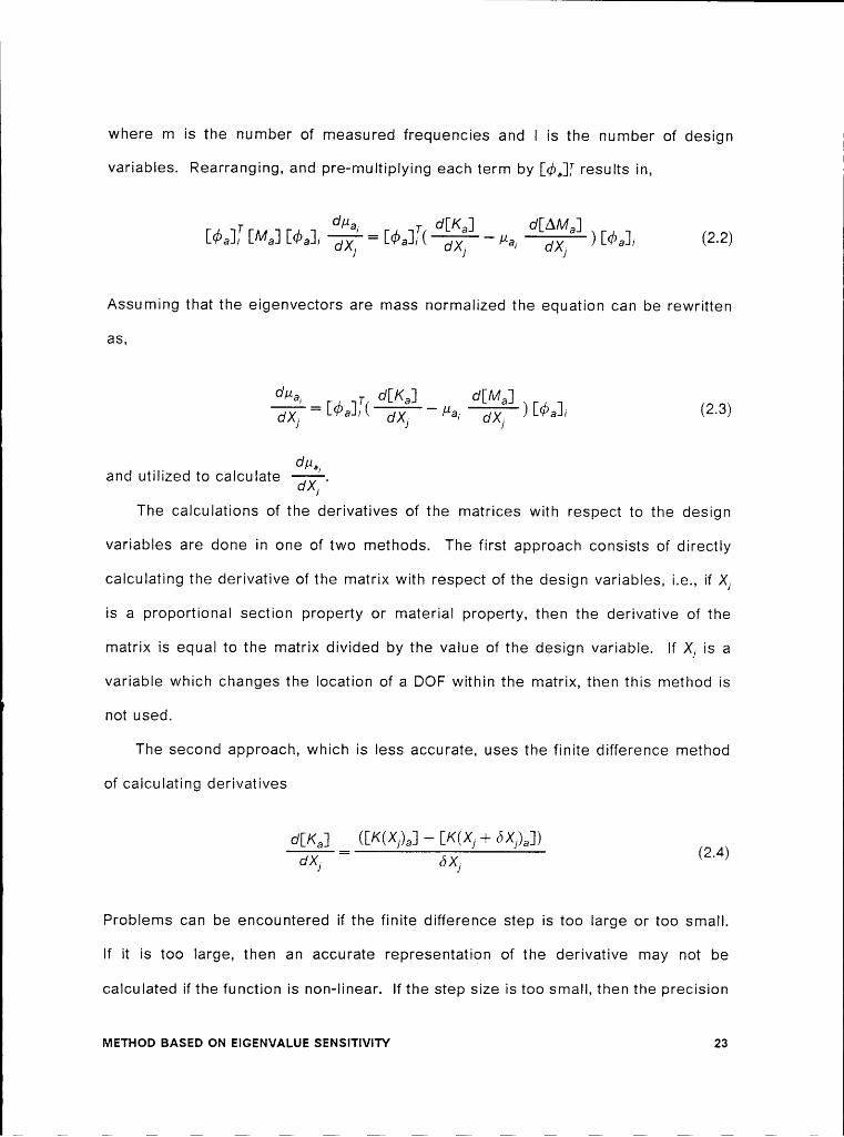
where m is the number of measured frequencies and l is the number of designvariables. Rearranging, and pre-multiplying each term by [gb,] results in,

du . d[K 3 6[AM 3T al[du]; Wa] #aT j) [du]; (2-2)

Assuming that the eigenvectors are mass normalized the equation can be rewritten

as,

¤'#a. T o'[K ] d[M ]

‘r d i d#°’and uti ize to ca culate GTX!.The calculations of the derivatives of the matrices with respect to the design

variables are done in one of two methods. The first approach consists of directly

calculating the derivative of the matrix with respect of the design variables, i.e., if XT

is a proportional section property or material property, then the derivative of the

matrix is equal to the matrix divided by the value of the design variable. lf XT is a

variable which changes the location of a DOF within the matrix, then this method is

not used.

The second approach, which is less accurate, uses the finite difference method

of calculating derivatives

d[/<a3 (l/<(XT)„] - [/<(XT + öXT)a]) T2 4)dXT — ÖXT '

Problems can be encountered if the finite difference step is too large or too small.

lf it is too large, then an accurate representation of the derivative may not be

calculated if the function is non-linear. lfthe step size is too small, then the precision

ME‘rHo¤ BAsE¤ ON EIGENVALUE sENslTiviTv 23

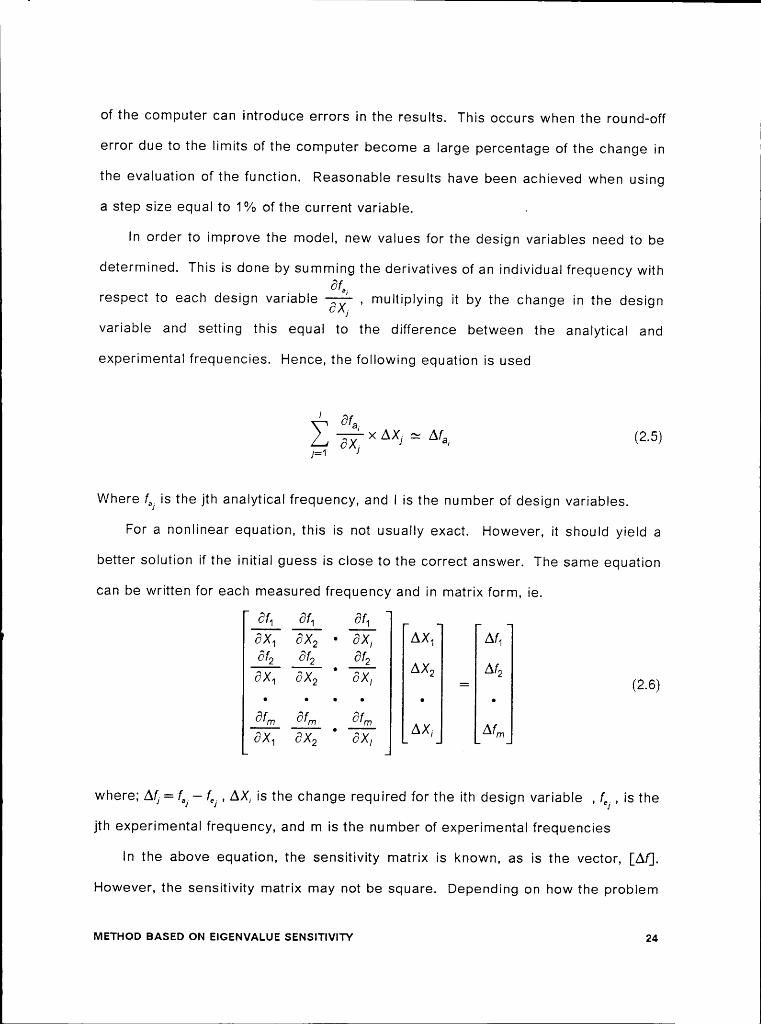
of the computer can introduce errors in the results. This occurs when the round-offerror due to the limits of the computer become a large percentage of the change inthe evaluation of the function. Reasonable results have been achieved when usinga step size equal to 1% of the current variable. -

In order to improve the model, new values for the design variables need to bedetermined. This is done by summing the derivatives of an individual frequency withrespect to each design variable , multiplying it by the change in the designvariable and setting this equal to the difference between the analytica! and

experimental frequencies. Hence, the following equation is used

’ ar,}.E X AX, z Ara, (2.5)

Where fa! is the jth analytica! frequency, and I is the number of design variables.

For a nonlinear equation, this is not usually exact. However, it should yield a

better solution if the initial guess is close to the correct answer. The same equation

can be written for each measured frequency and in matrix form, ie.

ii EL EiÖX1 ÖX2 ° ÖX, AX1 At'1öf öf öf

öf öf öf AX, Ar„,

where; AQ = faj — fe] , AX, is the change required for the ith design variable ,f,.j, is thejth experimental frequency, and m is the number of experimental frequencies

In the above equation, the sensitivity matrix is known, as is the vector, [Af].

However, the sensitivity matrix may not be square. Depending on how the problem

iviE*ri~iob BASED ou EIGENVALUE ssusmvrrv 24

l

is defined and what assumptions are made, the problem can be either under lconstrained or over constrained. lf the problem is over constrained, then a least

squares fit can be used to solve for [AX]. lf the problem is underconstrained, then

there are different solution techniques that can be used. Equations can be added tothe system of equations to make it square. These equations can be in the form of

requiring that the sum of the mass be constant, that the ratio of the masses be

constant, or the ratio ofthe individual components ofthe mass and stiffness matrices

be constant.

The problem is nonlinear, therefore it requires an iterative solution. An initial

eigensolution is performed, the sensitivity values are calculated, then a new [X]

vector is generated. This procedure is the repeated with the new [X] vector until theresults fall within a predetermined margin of error, Q ,

[XL1 = [X]; — [AX], (2-7)

where, [X] is the vector of design variables. The procedure is repeated with new

design variables until

[AUT [AU g Q (2.8)

2.3 Implementation

The implementation ofthis method is fairly straight forward. However, it requires

a good understanding of Direct Matrix Abstraction Programming (DMAP) and program

flow in MSC/NASTRAN. The direct method of calculating matrix derivatives is used

MET!-lob BASED ON Eic-ENvAi.uE sENsiTiviTY 25

ll

instead of the finite difference approach. This makes the method quicker and is easyto do for simple problems. The solution sequence from MSC/NASTRAN’s design

sensitivity analysis (Solution 53) could have been used for a more difficult problem.

Once the individual sensitivities are calculated they are assembled into a

sensitivity matrix. Additional equations are added to make the sensitivity matrixsquare. These equations depend on constraints supplied by the user and depend on

the number of frequencies measured.

Appendix A.1 lists the program used to solve the free-free beam problem with 6

modes used in the identification process. Following is a step-by-step explanation of

the alterations required for this method.

1.) The initial statements set up the NASTRAN run and initialize a database for

storage.

2.) Store Matrix derivatives in database: These statements store the previously

determined matrix derivatives in the database in a subscripted fashion. lf they were

not previously calculated this is where they could determined using sensitivity

analysis.

3.) lnitialize and rename matrices: section renames matrices and internally sets

some matrices to be able to be appended to, so that the dimensions of the matrices

can change.

4.) Top of iterative loop: This is the top of the loop for iterative calculations of

the objective function and Newton—Raphson iteration.

5.) Perform eigenvalue analysis: Performs eigenvalue analysis using current

mass and stiffness matrices.

6.) Generate analytical and experimental frequencies: This section extracts the

frequencies and eigenvalues and puts them in a useable form for later use.

MET!-lob BASED ON EIGENVALUE SENSITIVITY 26

I

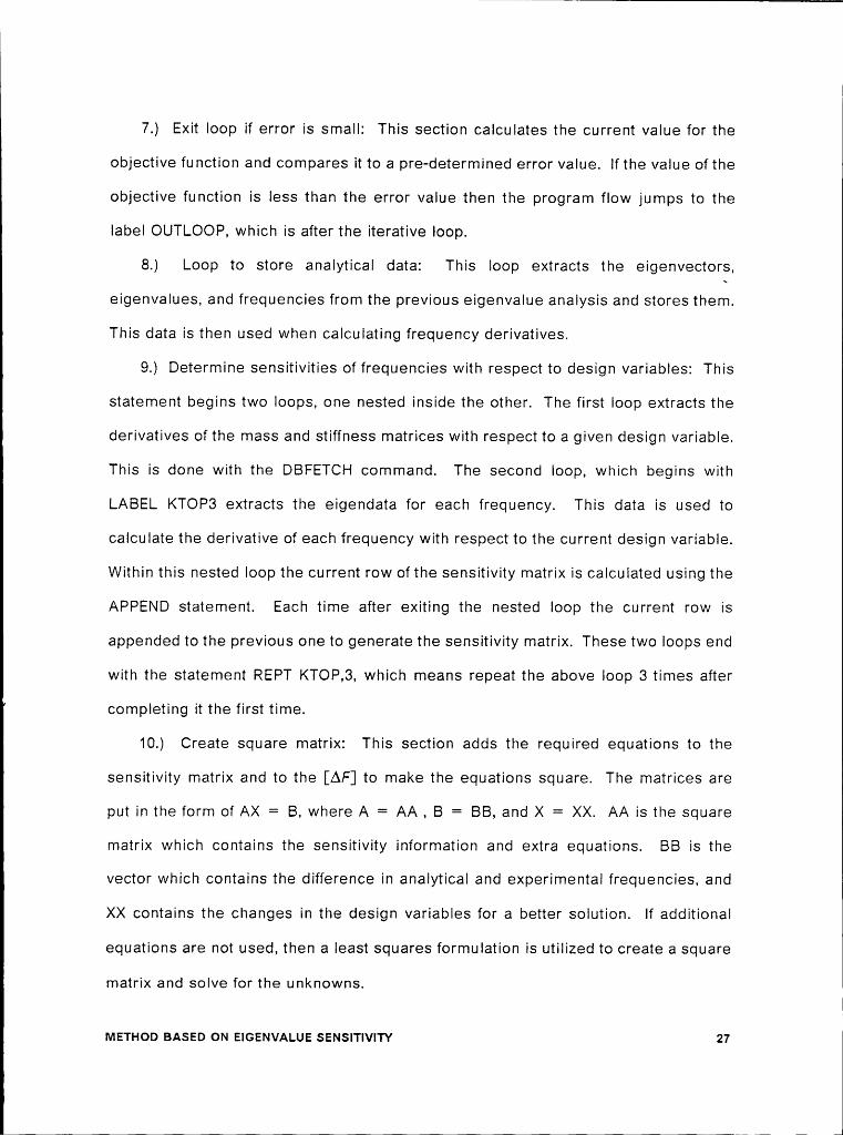
7.) Exit loop if error is small: This section calculates the current value for theobjective function and compares it to a pre-determined error value. lf the value ofthe

objective function is less than the error value then the program flow jumps to the

label OUTLOOP, which is after the iterative loop.

8.) Loop to store analytical data: This loop extracts the eigenvectors,

eigenvalues, and frequencies from the previous eigenvalue analysis and stores them.

This data is then used when calculating frequency derivatives.

9.) Determine sensitivities of frequencies with respect to design variables: This

statement begins two loops, one nested inside the other. The first loop extracts the

derivatives of the mass and stiffness matrices with respect to a given design variable.

This is done with the DBFETCH command. The second loop, which begins with

LABEL KTOP3 extracts the eigendata for each frequency. This data is used to

calculate the derivative of each frequency with respect to the current design variable.

Within this nested loop the current row ofthe sensitivity matrix is calculated using the

APPEND statement. Each time after exiting the nested loop the current row is

appended to the previous one to generate the sensitivity matrix. These two loops end

with the statement REPT KTOP,3, which means repeat the above loop 3 times after

completing it the first time.

10.) Create square matrix: This section adds the required equations to the

sensitivity matrix and to the [AF] to make the equations square. The matrices are

put in the form of AX = B, where A = AA, B = BB, and X = XX. AA is the square

matrix which contains the sensitivity information and extra equations. BB is the

vector which contains the difference in analytical and experimental frequencies, and

XX contains the changes in the design variables for a better solution. If additional

equations are not used, then a least squares formulation is utilized to create a square

matrix and solve for the unknowns.IMET!-lob BASED ON Eic;ENvALuE SENSITIVITY 27

11.) Solve system of equations: This statement solves for XX in the previouslymentioned equation.

12.) Extract components of XX (Delta X) vector: This section extracts the values

from the XX vector for use as multipliers when creating new design variables.

13.) Assemble new mass and stiffness matrices: This section generates new

mass and stiffness matrices, by using the new design variables.

14.) Repeat iterative loop 5 times: This is the end ofthe iterative loop which tells

the program to execute the loop 6 times, if the objective function has not obtained alow enough value.

The rest of the program is data used for setting up the analysis in NASTRAN.This procedure assumes that the matrix derivatives are calculate directly. Step

9) would not be changed by calculating the derivatives by finite difference. The

step-by-step procedure would need to be modified previous to step 1). This would

involve utilizing the solution sequence 53 (sensitivity analysis) from l\/ISC/NASTRAN.

One could either do a previous run and calculate the derivatives and store them in

the database, or one could include solution 53 (slightly modified) in the program

listed in the appendix.

METHOD BASED ON EIGENVALUE SENSITIVITY 28

Chapter lll

3.1 Introduction

The previous chapter detailed a technique which utilized an iterative approach to

update the system matrices. Berman and Nagy’s (1983) modification method, which

is developed in this chapter, yields a closed form solution. Their approach relies on

utilizlng constraint equations which are associated with normal modes analysis.

Normal modes analysis implies a system which is undamped and unforced. They

attempt to satisfy the orthogonality of the measured modes to the analytically derived

system matrices, while minimizing the changes to the mass and stiffness matrices.

Their paper is probably the most referenced of all of the papers dealing with the

METHOD THAT UTILIZES ORTHOGONALITY EQUATIONS 29

existing methods. More recent techniques utilize some of its characteristics while

others use it to compare new methods.

Often there are more coefficients in the analytical matrices than there aren

measured data. The experimental data consists of modal parameters; i.e.

frequencies and modes shapes. If this is the case, then the natural frequencies and4

modes shapes can be represented by a new eigenvalue problem, which results from

the updated mass and stiffness matrices. An advantage ofthis technique is that there

is no initial eigensolution required, and the method offers a closed form solution, and

the updated system matrices are symmetric.

There are also less desirable attributes ofthis method. The matrices are globally

modified, meaning that all coefficients of the matrices can be modified even if they

are already correct, or zero. l\/lodifying matrix coefficients that were originally zero

is similar to adding new members or elements to the model. This will usually result

in non-physically correct models. In addition, new eigenvalues can be introduced

when utilizing this technique (Ibrahim and Saafan,1988).

In order to modify the mass matrix an error function must be set up which utilizes

the orthogonality condition of normal modes. This function is minimized using

Lagrange multipliers. From this an updated mass matrix is developed. The stiffness

matrix can also be modified using the eigenvalue equation with the updated mass

matrix. An error function, comprised of changes to the stiffness matrix, is minimized

while using Lagrange multipliers for the eigenvalue constraint equation.

IMETHoo THAT UTILIZES ORTHOGONALITY EQUATIONS 30 I

3.2 Development

This method can be applied using a set of analytical system matrices along with

a set of experimentally derived natural frequencies and corresponding modal vectors.

Berman and Nagy assume that the mass matrix is more accurate than the stiffness

matrix. lt is usually easy to determine the total mass of a system, and it is only

somewhat more difficult to determine the distribution of that mass throughout the

structure. Whereas, it is more difficult to determine a lumped stiffness value for a

continuous system. Hence, the mass matrix is corrected with the modal matrix, then

the stiffness matrix is adjusted with the use of the frequencies, modal matrix, and the

updated mass matrix.

The modification ofthe analytical mass matrix is accomplished assuming that the

experimental modal matrix is correct, and that experimental data is available at every

analytical DOF. lf this is not the case, then the analytical matrices can be reduced to

match the experimental data, or the experimental data can be expanded to match the

analytical model.

The mass matrix is updated in order to make the matrices and experimental data

compatible. All of the modal vectors are assumed to be mass normalized, i.e.

1t¤ m (3-1)

where, m is the number of measured modes. However, the experimental modes may

not be orthogonal since;

may not equal O for i ¢j

METHOD THAT uTii.izEs ORTHOGONALITY EQUATIONS 31

where, [due], is the ith experimental modal vector, and [Me] is the analytica! massmatrix.

Berman defines AM to be equal to the difference between the analytica! mass

matrix and the updated mass matrix.

[AM] = [MU] — [Ma] (3-2)

Hence the orthogonality relationship can be expressed as

U] (3-3)

By separating the equation and rearranging it

le]TlA/W] [38] = U] — [ma] (3-4)

where, [me] is defined as

[ma] = le]T[Ma] übe] (3-5)

Equation (3.4) implies that [due]’[AM] [due] contains only the negative of the

off-diagonal terms defined by [due]T[Me] [due] .

An error function is set up such that utilizes a mass weighted minimization of the

percent changes to the mass coefficients

3 = ii r~1"rA)71r~1" ii (3-5)where || || denotes using the Einstein rule of summation

fi fl

6 = Z 2([^/]'°[A^/Y] r~)" )$ (3-7)i=1 j=1

METHOD THAT uTii.izEs ORTHOGONALITY EQUATIONS 32

n is the number of DOF in the model, and N is defined as

rm (2-2)A Lagrangian multiplier Ä,) , is used for each matrix coefficient of eq. (3.4). The

Lagrange multipliers are used to incorporate constraints while minimizing the

percent change to the components ofthe analytical mass matrix, while modelling the

modal data correctly. The Lagrangian function is then set up

/Tl /'/7

1// = 2 E/J + [1%]),, (3-9)/=1j=1

where m is the number of measure modes. Equation (3.9) is differentiated with

respect to each component of [AM], and each derivatlve is set equal to zero, i.e.,

dw n n n n m m2ZZ[fs /:1 j=1 k=1 /:1 /:1 j:1

where, AM,s corresponds to the coefficient of [AM] in the rth row and sth column.

This results in a

2 [/1/a]—1[A/V/J L1/.1* + = 1) (3-11)

or

1[AM] = — -5 [Ma] [dn,] [A]Tl</>e]T[/Wa] (3-12)

METHOD THAT UTILIZES ORTHOGONALITY EQUATIONS 33

l

V\/here A contains the Lagrangian multipliers Ä,) . Equations (3.4) and (3.12) containonly 2 matrix unknowns [AM] and [A] .

By substituting eq. (3.12) into eq. (3.4), [A] is then determined to be

[A] = [A]T = -2 [ma]’1([/] - [m,..]) [m,]‘1 (3-13)

A is symmetric, because of the symmetry of eq. (3.5), i.e., the off diagonal terms of

[q5„]’[M,] [cb,] are equal. Equation (3.13) requires the inversion of [ma] . This matrix

is a function of the analytical mass matrix and the experimental modal vectors. ln

general [ua] is not singular even if [M,] is singular. This is due to the arithmetic

process of carrying out the triple product of the modal vectors and mass matrix (see

eq. 3.5). lf the modes are orthogonal, this is apparent as [ma] will be a diagonal

matrix with no zero terms on the diagonal. However, if the quality of the modes is

not high, [ma] is not guaranteed to be non-singular. By substituting eq. (3.13) into eq.

(3.12), [AM] is determined to be

[AM] = [Ma] [du-] [m,,]'1([/] - [ma]) (3-14)

The updated mass matrix can be obtained by recalling from eq. (3.2) that

[M.,] = [M,] + [AM] (3-15)

Thus a closed form method of updating the mass matrix can be performed. This

method assumes that the modal matrix is correct and that the mass matrix should be

modified to make the modes normal. This is done without an eigensolution and

minimizes changes to components of the mass matrix. However, all of the

coefficients of the mass matrix can change. Thus, the compatibility of the finite

METHO¤ THAT UTILIZES 0RTHOc0NALlW EQUATIONS 34

lelement model is not conserved. The resulting modal matrix and mass matrix are

compatible, in that the triple product of the modal matrix and the mass is equal to the

identity matrix.

The updated mass matrix and the eigendata are used to modify the analytical

stiffness matrix. This is accompllshed using three constraint equations which are

based on; the eigenvalue equation, the orthogonality relations, and the enforced

symmetry of the stiffness matrix;

[KU] [¢>6]—[/17,,] [¢>6] [#6] = 9 (3-13)

[<l>6]T [K6][<¢>6] — [#6] = 9 (3-17)

[KU] — [K„]T = 9 (3-13)

An error function is set up similar to the one used for the mass matrix

modification,

6 = Il [^/]'1([K„] — [K6]) [^/]°1 ll (3-19)

Three Lagrangian matrices are required for the constraint equations

([A„],[AO],[A$]). The Lagrangian equation can then be set up as

iv = 6 [M6] [<1>6] [#6]),, +1=1 j=1

I7 flm m(3-20)

/:1 j=1 i=1 J.=1

METHOD THAT UTILIZES ORTHGGONALITY EQUATIONS 35

77 Y V

YIna similar manner to the derivation of the mass matrix modification, equation (3.20)

is differentiated with respect to the components of the updated stiffness matrix and

set equal to zero.

Thus results in an updated stiffness matrix of

[K.,] = [K,.] + ([A] + [A]T) (3-21)

where

1[A] = -5 [K.,] (3-22)

The stiffness matrix is modified without an eigensolution using the updated mass

matrix and the eigendata. However all coefficients of the stiffness matrix can be

modified.

3.3 Implementation

This method is straight-forward to implement within MSC/NASTRAN. The

eigendata is entered into the program via Direct Matrix Input (DM!) cards in the bulk

data deck in normalized form. The system matrices are assembled within solution

63 (Normal modes analysis). Appendix A.2 provides a listing of the program used in

the identification process for the free-free beam using 6 modes. Following is a

step-by—step explanation of the alterations ofthe program, required to implement this

method.

METHOD THAT UTILIZES oRTHoGoNAL!TY EQUATIONS 36

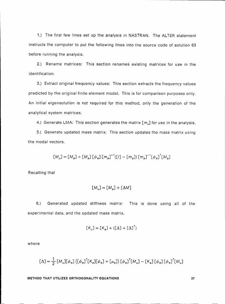
1.) The first few lines set up the analysis in NASTRAN. The ALTER statement

instructs the computer to put the following lines into the source code of solution 634

before running the analysis.

2.) Rename matrices: This section renames existing matrices for use in the

identification.

3.) Extract original frequency values: This sectionextracts the frequency values

predicted by the original finite element model. This is for comparison purposes only.

An initial eigensolution is not required for this method, only the generation of the

analytical system matrices.

4.) Generate Ll\/lA: This section generates the matrix [ma] for use in the analysis.

5.) Generate updated mass matrix: This section updates the mass matrix using

the modal vectors.

[MU] = [M9] +

[M9]Recallingthat 4

[Mu] = [Ma] + [AM]

6.) Generated updated stiffness matrix: This is done using all of the

experimental data, and the updated mass matrix.

[KU] = [K9] + ([A] + [A]T)

where

1[A] = 5 [M„][<1>9] ([<l>9]T[K9][9] + [#9]) [d>9]T[^/lu] — [K9] [¢>9] [<l>9]T[M„] l

METHOD THAT UTILIZES ORTHOGONALITY EQUATIONS 37 ‘

7.) Extract newly calculated eigenvalues and eigenvectors: This sectionperforms and eigenvalue analysis using the updated system matrices and extracts

the values for comparison. _

8.) Print results: This section prints the results extracted during the computation.

The rest of the input is the required data to set up the NASTRAN analysis.

METHo¤ THAT UTILIZES ORTHOGONALITY EQUATIONS 38

Chapter IV

Il/IETHOD BASED ON CONNECTIVI I Y CONSTRAINT

4.1 Introduction .

A goal of System Identification is to generate a system which accurately predicts

the response of a structure to an input. Of interest, is to also keep the mathematical

system physically realistic. This can be done by applying additional constraints; i.e.

no change in overall mass, similar connectivity relationship as the initial model, or

making element byelement change only.

The method developed in this section utilizes a closed form technique, and does

not require a previous elgensolution in order to perform the matrix modification.

Kabe’s method (1985) utilizes a constraint relationship that implies that no new load

paths should be introduced to the structure. This implies that all matrix coefficients

that were originally null, must remain null in the final matrix.

MET:-ioo 6AsEo ou connectivity coNsTRAi~T as

Kabe’s method minimizes the percent change to the coefficients of the stiffness

matrix. The method assumes that the mass matrix is reasonably correct, because

mass is something that can be directly measured. Therefore, it is more important to

modify the stiffness matrix than the mass matrix.

His formulation assumes that the modes are orthogonal. However, results can

be obtained if they are not. Different methods, similar to the one used for the

orthogonality method can be used to make the modal vectors compatible with the

mass matrix. Kabe utilizes Lagrange multipliers to mlnimize an error function

comprised of relative changes to the original stiffness matrix, while adhering to

certain constraints. This method yields a closed form solution.

4.2 Development

Kabes method modifies the global stiffness matrix using a connectivity constraint

and minimizing the relative change to the components of the analytical matrix. His

method does not require an initial eigensolution, only the formulation ofthe analytical

system matrices, and the experimental data.

Kabe assumes that the mass matrix is reasonably correct. He wants to base the

modification method on defining the stiffness matrix as accurately as possible. This

is due to the fact that the structures being modelled may eventually have added

mass, due to loads they will be carrying. He requires that the updated stiffness

matrix be defined as

[Ku] = [Ka] · Ev] (44)

lviE‘ri-lob BAsE¤ ON coNNEcTivlTv coNsTRAiNT 40

i

l

Where • implies that the components of both matrices be multiplied by each

other, i.e.

Ku,} = Ka,] Vi] (42)

This constraint implies that no new load paths will be introduced to the model.

lf Kajj = 0 then Kuij = O as well.

An error function is set up which contains the relative change to each stiffness

coefficient:

f7 I7

¤ = E E ia, — /„ V„> (4-3)l=’l j=‘l

where n is the number of DOF in the model,

[J =1 if Kai! ¢ 0 (4.4)

/\/U = O if Kai] = O (4.5)

The adjusted stiffness matrix is determined by finding the [y] which minimizes 6

while obeying the following constraints. The eigenvalue equation

·— [M8] [$8] [#8] + ([/<8] · [V]) [$8] = O (4-6)

and the symmetry of the updated stiffness matrix

[V]- [V]T = O (4-7)

METHOD BASED ON CONNECTIVITY c0NsTRA|NT 41

The method of Lagrangian multipliers is used to minimize 6 while adhering to theconstraints defined by eq (4.6) and (4.7).

T7 VT7fl fl ry11 = E — 1//1 111.1 111.1 1,)1:11:1 _ 1:11:1 }=‘l

where, m is the number of measured frequencies.

The partial derivative of 1,/1 is taken with respect to each y,,, and these equations

are set equal to zero.

Taking the derivative of 6 with respect to y,, results in

f7 fl" A A A ÖV".%.:22 2 (1-}..},..) 1.-l (4 g)öyrs /:1 /:1 /1 /1 /1 /1 öyrs

Noting that:

ÖV/1 . . .-;—=0 1f1;érorj;és0Vrs

6/11 . . .—,7——=’l IfI=/’aTldj=S0Vrs

This results in

^ A A</rs-/rsrs

Taking the derivative of

METHOD BASED ON CONNECTIVITY CONSTRAINT 42

l

l

n m n

i=1 j=1/:1

yields

m2/l”rJKar=d) evj=‘l

Taking the derivative of [M] [cb,] [ii,] yieids zero. Taking the derivative of

n n“ Vj;)

·;’=‘l j=1

yields

ÄSISi

Ässr

The resulting equation in matrix form yields

— 2([/] — [vl) + [Ka] •([^„] [<1>e]T)+ [AS] = 0 (4-11)

Noting that

[As] + [^s]T = O (4-12)

from the symmetry condition, [A,] can be eliminated from eq (4.11) by adding the

transpose of the equation to itself, yielding

l

— 4([7] — tn) + [KS] ·(tAS1 L-4,17 +64,1 tASJT)= ¤ (4-18)

Equation (4.13) can be pre-multiplied element by element by [K8] and

rearranged to form

KKS] • Kv] = KKS] (KAS] K<1>S]T + K<1>S] KAS]T) (4-14)

where,

K<!>] = KKS] · KKS] (4-15)

and noting that

[K8] . [7] = [K8] (4.16)

By combining eq. (4.6) and (4.14), these yield

KA] + (K] • (KAS] KS]T)) K<l>S] + (K<l>] • (K¢>S] KAS]T)) K<bS] = 8 (4-17)

where,

KA] = 4 KMS] Ku.-,] — KKS]KS] (4-18)

ln order to solve eq (4.17) for A8 , we define [A] as a column vector containing all of

the transposed rows of [A]. [A] is a n by m matrix and [A] is an (n x m) by 1 matrix.

For example, for the case when [A] is a 3 by 2 matrix:

METHOD axxsso ou couuscrivlrv coNsTRAiNT 44

A11A12

A11 A12- A21

[A] = where [A] = A21 A22 (4.19)A22

A31 A32A31

A32

Simllarly [XS] as

A11

A12_ A11 A12— A21[As] = where [AS] = 2.21 2.22 (4.20)

A22_ A31 A32

A31A32

Recalllng that • means element by element multipllcatlon, ([<D] ~ ([A,] [d>2]’)) [¢>2] can

be rewritten as

Ol'

n

/=1

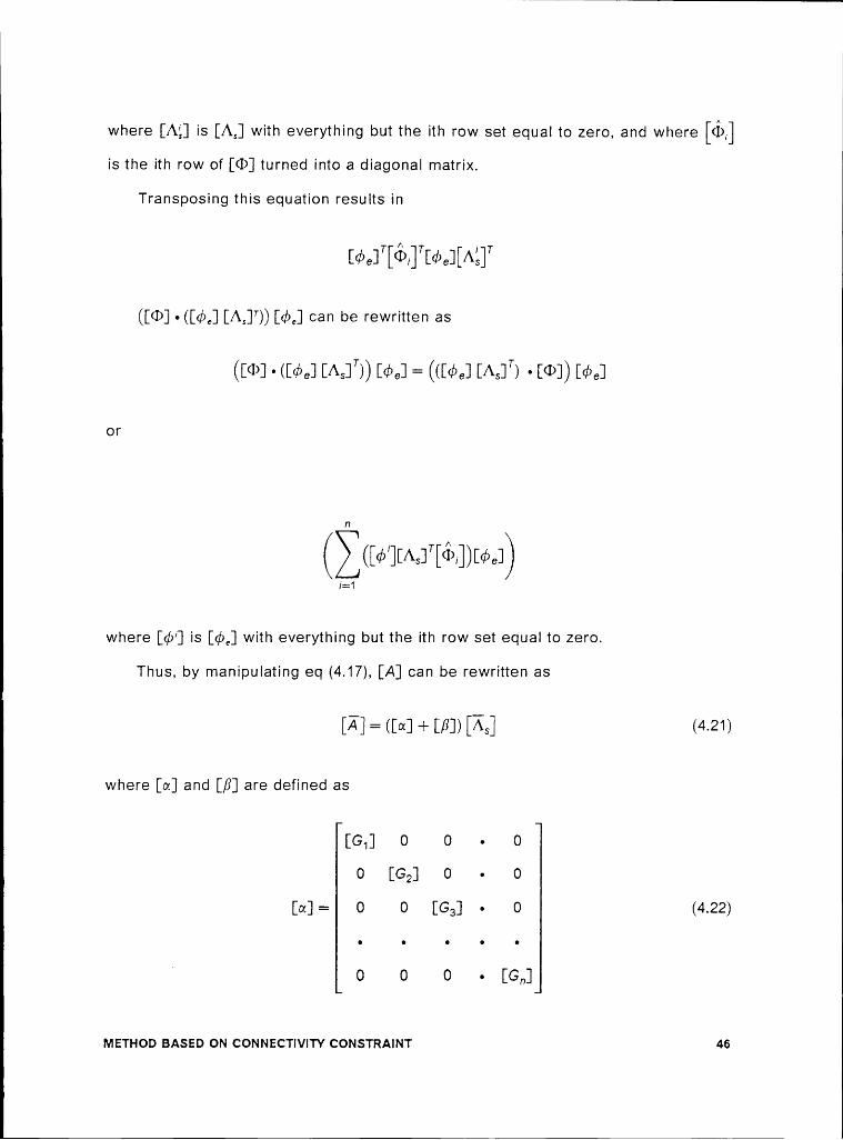
where [AQ] is [A,] with everything but the ith row set equal to zero, andwhereis

the ith row of [CD] turned into a diagonal matrix.

Transposing this equation results in

r¢»..1'[<i5,]’rz>,1[A;]'([CD] • ([zb,] [A,]')) [zb,] can be rewritten as

(UD] • (übe] [^S]T)) [dw] = (([d>6] [^$]T) • [<l>]) [be]

Ol'

i=1

where [zb'] is [zb,] with everything but the ith row set equal to zero.

Thus, by manipulating eq (4.17), [A] can be rewritten as

[Ä] = (K4] + Eßl) [K.] (4-21)

where [oz] and [ß] are defined as

[6,] 0 0 „ 00 [62] 0 • 0

[Q] = 0 0 [63] • 0 (4.22)

1 0 0 0 • [6,,]

man-soo aAsE¤ on connscnvmz cousnmmr 46

[/*/11] [/*/12] [/*/12] • [/*/1,1] l[//21] [/*/22] [//22] • [/*/2,1]

[ß] = [//21] [H22] [/*/22,] · [/*/2,1] (4-23)

[*/:11] [//Z12] [/*/;,2,] [/*/;,,1] I

where

[6,1 = — [4.1/ [,]t«l>.-,1 (4.24)

and

[4)),] is a diagonal matrix whose elements are the ith row of of [<l)]

and where

[/*/],) = — [D,][ (4-25)

and

[0,],: ith column of [168]/ [<]>,] (4.26)

[E5], : un column of [d>e]T (4.27)l

Equation (4.21) can be solved by defining the following transformation,

[K.] = rw rp] (4-28)

lvllsrnou aAss¤ ON CONNECTIVITY CONSTRAINT 47

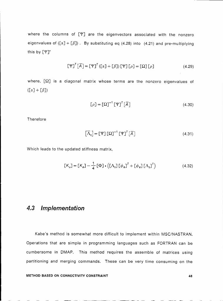
ilwhere the columns of [T] are the eigenvectors associated with the nonzero

eigenvalues of ([0:] —l— [8]) . By substituting eq (4.28) into (4.21) and pre-multiplying

this by [TY

[‘I’]T [Ä] = [‘V]T (Dx] + [,3]) [T] Dx] = [92] Dx] (4-29)

where, [Q] is a diagonal matrix whose terms are the nonzero eigenvalues of

([¤] +[ß])

Dx] = [QT] [‘Y]T [Ä] (4-33)

Therefore

[K.] = wi rsxrl rw [Ä] (4-31)

Which Ieads to the updated stiffness matrix,

1 r rD<„]=[K.,]—j,·[<1>]·([^S][<xx.] +D1>6]D\S] ) (4-32)

4.3 Implementation

Kabe’s method is somewhat more difficult to implement within l\/ISC/NASTRAN.

Operations that are simple in programming languages such as FORTRAN can be

cumbersome in Dl\/IAP. This method requires the assemble of matrices using

partitioning and merging commands. These can be very time consuming on theivnrruoo 6AsE¤ ou conuscrivrrv coNs·rnA¤N‘r48]___.__ _ ._ ._-e._%.-_ 2.._._... -1

l

computer. Due to the fact that only non-zero eigenvalues of ([ot] + [,6]) are used, andthe number ofthese may be unknown, the analysis may need to be run for a different

number of non-zero eigenvalues. Appendix A.3 contains a listing ofthe program used

to solve the free-free beam using 6 modes in the identification process. Following is

a step—by-step explanation of the alterations required to implement this method.

1.) The first few lines set up the initial analysis in NASTRAN. The ALTERstatement teils the NASTRAN to include the next statements with the source code.

2.) Store matrices: This section renames current matrices for later use.

3.) Generate experimental eigenvalues: This section converts the experimental

frequencies into eigenvalues.

4.) Generate A: This section generates the matrix [A] .

5.) Generate cap phi from original K matrix: This section computes [<D] by

multiplying the stiffness matrix element by element by itself.

6.) Generate partition vectors: ln order to partition or merge certain matrices

within NASTRAN, there must be a vector which defines how the vector should be

partitioned or merged.

7.) Set up loop to generate matrices: This section starts a loop which executes

the number of times there are DOF in the model.

8.) Extract rows from cap phi: This section extracts each row from [<D] and

converts it into a diagonal matrix.

9.) Generate A bar from A: This section converts matrix [A] into [A] .

10.) Generate G sub i: This section generates each [G,] .

11.) Generate ephr#: This section extracts each row of the modal matrix and

turns it into a column.

12.) Generate l\/l##: This section generates the lVll\/ll\/l matrix used in later

calculations.

METHOD BASED ON CONNECTIVITY coNsTRAlNT 49

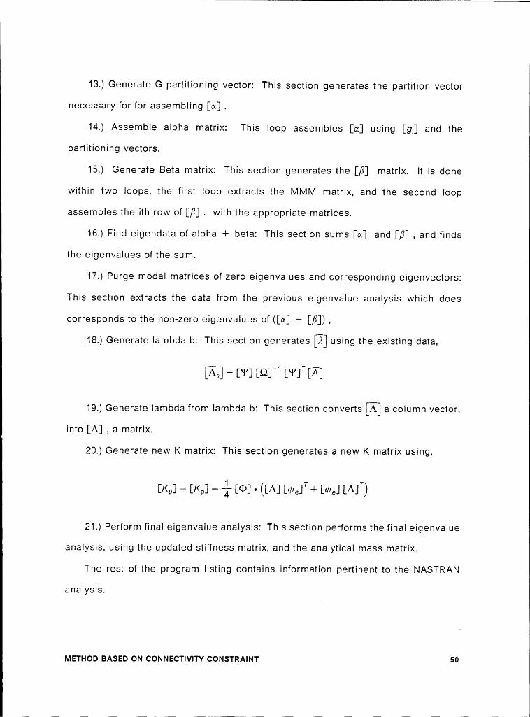
l

13.) Generate G partitioning vector: This section generates the partition vectornecessary for for assembling [oe] .

14.) Assemble alpha matrix: This loop assembles [or] using [g,] and the

partitioning vectors.

15.) Generate Beta matrix: This section generates the [ß] matrix. It is done

within two loops, the first loop extracts the l\/ll\/ll\/l matrix, and the second loop

assembles the ith row of [ß] . with the appropriate matrices.

16.) Find eigendata of alpha + beta: This section sums [ot] and [ß] , and finds

the eigenvalues of the sum.

17.) Purge modal matrices of zero eigenvalues and corresponding eigenvectors:

This section extracts the data from the previous eigenvalue analysis which doescorresponds to the non—zero eigenvalues of ([rx] + [,8]) ,

18.) Generate lambda b: This section generates using the existing data,

{K.] = L—W Lm" LW LZ}

19.) Generate lambda from lambda b: This section converts [A] a column vector,into [A] , a matrix.

20.) Generate new K matrix: This section generates a new K matrix using,

(KA]21.)Perform final eigenvalue analysis: This section performs the final eigenvalue

analysis, using the updated stiffness matrix, and the analytical mass matrix.

The rest of the program listing contains information pertinent to the NASTRAN

analysis.

NIETHOD BASED ON CONNECTIVITY CONSTRAINT so

il

Chapter V

METHOD BASED ON RESIDUAL FORCE VECTOR

5.1 Introduction

In both experimental and analytical results, errors exist. The object of System ’

identification is to identify the best system. Finite Elements methods are developed

based on certain assumptions. It is rare that these assumptions are 100% correct in

the entire model. Through various techniques it is possible to determine where

errors in the analytical model may exist. By correcting the model in this area only,

one may be able to generate a good model which is also physically meaningful.

The method implemented in this chapter utilizes residual force vectors. lt was

developed by Chen and Wang (1988). A residual force vector is a vector which results

from subtracting two quantities, which calculate forces, from each other. Due to the

discrete nature and assumptions of finite elements, as well as errors in the

experimental error, residual forces will usually result. By examining these forces one

ivisrnoo aAsEo on RssiouAi. i=oRcE vEc‘roR 51

l

l

lshould be able to locate modelling errors in a model. Once these locationsareknown,

then one can modify these locations in order to update the analytical model

using test data.

Chen and Wang introduce a method for calculating the residual force vector.They then offer different approaches to updating the analytical model using this

information. The three approaches offered are based on; (1) the orthogonality

approach, (2) the re-analysis approach, and (3) the statistical approach.

The method developed in this chapter is one which uses the orthogonality

approach. Their method attempts to find matrices which when added to the analytical

matrices will solve the eigen problem more accurately. The new matrices are

comprised of contributions from elements around the location of modelling errors

only. Therefore, this method enforces element connectivity, and matrix symmetry.

5.2 Development

The model refinement method described by Chen and Wang is divided into two

parts. Their initial concern is to locate modelling errors in the analytical model. This

is accomplished by finding locations in the model where forces do no sum to zero.

Their second concern is to modify the matrices utilizing information obtained from the

error location procedure.

The eigenvalue equation is manipulated in order to find the location ofthe errors.

In theory

—[^/16] [$6], #6, + [K6] [$6], = 0 (5-1)

METHOD BASED ON RESIDUAL FORCE VECTOR 52

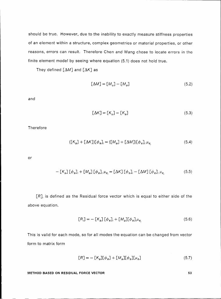
should be true. However, due to the inability to exactly measure st·iffness propertiesof an element within a structure, complex geometries or material properties, or other

reasons, errors can result. Therefore Chen and Wang chose to locate errors in the

finite element model by seeing where equation (5.1) does not hold true.

They defined [AM] and [AK] as

[AM] = [Mu] — [Ma] (5-2)

and

[AK] = [KU] - [Ka] (5-3)

Therefore

(U2] + [Al<])ld>6]/ = (W.-,-J + [A^4J)[<(>e]„ /L.-, (5-4)

or

#9/

#9/[R],is defined as the Residual force vector which is equal to either side of the

above equation.

[R,] = — [Ka] [<1>e],+[/Vla][<1>,,],//6, (5-5)

This is valid for each mode, so for all modes the equation can be changed from vector

form to matrix form

[R] = — [/<a][<z>.,] + E/Vla][d>..-JT/J6-J (5-7)

MET!-lob BASED ON RESIDUAL FORCE VECTOR 53l

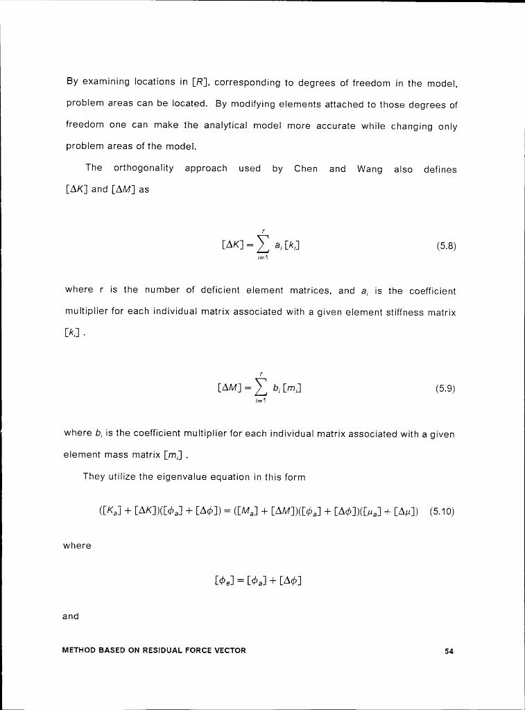
By examining locations in [R], corresponding to degrees of freedom in the model,

problem areas can be located. By modifying elements attached to those degrees of

freedom one can make the analytical model more accurate while changing only

problem areas of the model.

The orthogonality approach used by Chen and Wang also defines[AK] and [AM] as

f

[AK] = (5-8)/:1

where r is the number of deficient element matrices, and a, is the coefficient

multiplier for each individual matrix associated with a given element stiffness matrix

[/<.] -

f'

[A^//] = br [mi] (5-9)/:1

where b, is the coefficient multiplier for each individual matrix associated with a given

element mass matrix [m,] .

They utilize the eigenvalue equation in this form

([/<a] + [AK])([6>a] + [A</5]) = (Wa] + [AM])([</58] + [A6>])([ua] + [A/¢]) (5-19)

where

[656] = [658] + [A65]

and

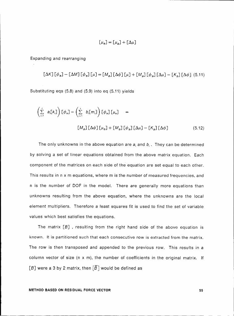
l

l

[#6] = [#6] + [A#]

Expanding and rearranging

[AK] [</>6] — [AM] [<1>6] [#] = [M6] [Ad>] [#] + [M6] [<1>6] [A#] — [K6] [Ad>] (5-11)

Substituting eqs (5.8) and (5.9) into eq (5.11) yields

(Z @[/6]) [<1>6]— (2 b,[m,]) [eb.] [#6] =1:1 /:1

[M6] [A</>] [#6]+ [M6] [¢>6] [A#] — [K6] [A<1>] (5-12)

The only unknowns in the above equation are a, and b,-. They can be determined

by solving a set of linear equations obtained from the above matrix equation. Each

component of the matrices on each side of the equation are set equal to each other.

This results in n x m equations, where m is the number of measured frequencies, and

n is the number of DOF in the model. There are generally more equations than

unknowns resulting from the above equation, where the unknowns are the local

element multipliers. Therefore a least squares fit is used to find the set of variable

values which best satisfies the equations.

The matrix [B] , resulting from the right hand side of the above equation is

known. It is partitioned such that each consecutive row is extracted from the matrix.

The row is then transposed and appended to the previous row. This results in a

column vector of size (n x m), the number of coefficients in the original matrix. lf

[B] were a 3 by 2 matrix, then [B] would be defined as

B11

B12B11 B12

- B21[B] = where [6] = 62, 622 (6.16)

B22B31 B32B31

B32

Similarly, this is done for each variable, or unknown matrix multiplier on the left

hand side of the equation. The resulting matrix [Q] is then (n x m) rows by (2r)

columns, where r is the number of deficient elements.

The resulting equation is

[G][Z] = [Ü] (5-14)

where [Z] contains the unknown matrix multipliers, and [Q] contains the columns

associated with the deficient elements.

This equation can be solved by pre—muItiplying each side of the equation by

[Q]T, and then pre-multiplying each side by ([O][[Q])*‘ . This assumes that

([Q]’[Q])—1 is not singular. The resulting equation is

t21= ([O]T[G])—1[G]T[§] (5.15)

lt should be noted that this is an ill conditioned solution method which may not

yield the desired the desired results for a large problem. The updated matrices are

obtained by,

ME‘rHo¤ BAsE¤ ON RESIDUAL FORCE vEcToR 56

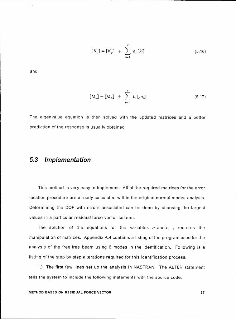
f

[Ku] = [Ka] + a,[k,] (5.16)I=’l

and

I'

WU] = [Ma] + E b, lm,] (5-17)i=1

The eigenvalue equation is then solved with the updated matrices and a better

prediction of the response is usually obtained.

5.3 Implementation

This method is very easy to implement. All of the required matrices for the error

location procedure are already calculated within the original normal modes analysis.

Determining the DOF with errors associated can be done by choosing the largest

values in a particular residual force vector column.

The solution of the equations for the variables a, and b, , requires the

manipulation of matrices. Appendix A.4 contains a listing of the program used for the

analysis of the free-free beam using 6 modes in the identification. Following is a

listing of the step—by—step alterations required for this identification process.

1.) The first few lines set up the analysis in NASTRAN. The ALTER statement

tells the system to include the following statements with the source code.

METH¤¤ BASED ON RESIDUAL FORcE vEcToR 57

l

2.) Rearrange matrices: This section rearranges, or renames matrices for usein the alteration.

3.) The following l\/!!\/!AT and Kl\/IAT : This section stores element matrices in

the database for use later in the analysis. These matrices are input by the user.

4.) Generate or rename experimental and analytica! data: This section puts the

existing data in a form to be used later.

5.) l\/lultiply each eigenvector by its eigenvaluez This section extracts each

experimental eigenvector and its corresponding eigenvalue and multiplies them

together. They are then reassembled into the matrix LPHI.[

6.) Calculate residual force matrix: This section calculates the residual force

matrix,

[R] = — [Ka][<l>e] + [/V!a][e][u]

The user must examine this matrix to determine where deficient elements exist in the

model.7.)

Calculate matrix for unknowns: This section calculates [B] , from

Wa] [M] fu] + [Ma] [du] [Au] — [Ka] [A4]

8.) Generate A matrix: This section calculates all possible columns needed for

[O] , using deficient element matrices. There is one column for each possible

unknown, a, or b,.

9.) Generate B matrix: This section calculates [B-] , from [B] .

10.) Extract columns corresponding to deficient elements: This section appends

each of the columns needed for [Q] , using deficient element matrices. There is one

column for each unknown, a, or b,.

l

11.) Solve for X using simple formulation: This section generates [Z] , the vector

of unknown matrix multipliers. lt then extracts the values and uses them to generate

new mass and stiffness matrices. An eigenvalue analysis is then performed with the

updated matrices.

12.) Print results: This section prints out the calculated data.

The rest of the program contains information pertinent to the NASTRAN analysis.


Chapter VI

NUIVIERICAL RESULTS

This chapter describes three numerical studies which were executed using the

four System Identification methods. The first study was a simple 2-DOF problem that

checked the validity of the developed methods. The second numerical study, which

is an 8-DOF example, was used to correlate the procedures to published studies. The

third study, utilizing experimental results from a free-free beam, details how the

methods work for an engineering problem.

6.1 Verification Studies - 2 DOF model

In order to assure that the methods were programmed correctly, they were

examined using a 2 DOF model. lt consists of 2 springs and 2 masses connected in

series, with the end of the first spring grounded (ref Figure 1 on page 62). These

Nuiviarucm. Rssuurs 60

verification studies include engineering problems as well as problems whichexamine the mathematical capabilities of the methods. For this thesis engineering

problems are defined as those which contain errors in the stiffness matrix only.

The "experimental" data used for the identification processes in this section isgenerated from the 2-DOF model, and this data is referred to as the

quasi-experimental data. The properties of the initial analytical matrices differ from

the quasi-experimental system matrices, thus the analytical results did not match the

quasi-experimental data exactly. By utilizing the four different System Identification

methods, the initial analytical models were updated using the quasi-experimentaldata. These updated system matrices were then compared to the original matrices

which yielded the quasi-experimental data. The frequencies and modal vectors that

the updated matrices yielded were also compared to the quasi-experimental data.

Table 1 on page 63 lists the properties used for the springs and masses for the

six 2-DOF test cases. The tests are called TEST 1a thru TEST 1f.

For each test there is a corresponding table (Tables 2 - 7) which contain the

matrices and modal data corresponding to the quasi-experimental data, as well as thefor the initial analytical model. Also included are the updated matrices resulting from

each method as well as the corresponding modal data.

The first four tests (TESTS a-d) consist of engineering tests, or problems whereonly the stiffness matrix is modified. The mass matrix in most analytical models is

assumed to be more accurate, as the mass of a structure can be determined

accurately, and the distribution of that mass throughout the structure can usually be

determined. \/\/hereas, the stiffness of a sub region of a model is more difficult to

specify.

The first two tests contain minor (10%) modifications to the springs. Table 2 on

page 65 contains the results of the first test in which the initial analytical model is

NUMERICAL RESULTS 61

K1 K2M1 M2

Fagum 1. 2 DOF SPRING MAss SYSTEM USED FOR EXAMPLE 1

NuMEmcA1. Rssuurs 62

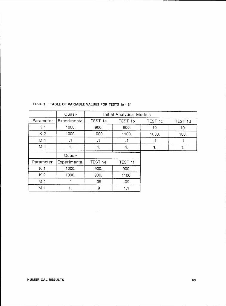
Table 1. TABLE OF VARIABLE VALUES FOR TESTS 1a · 1f_

Quasi- lnitial Analytical ModelsParameter Experimental TEST 1a TEST 1b TEST 1c TEST 1d

K 1 1000. 10. 10.K 2 1000. 1000. 1100. 1000. 100.M 1 .1 .1 .1 .1 .1M 1 1. 1. 1. 1. 1._

@1*85** —Parameter Experimental TEST 1e TEST 1f1<1K

2 1000. “ 1100.M 1 -1 til' M 1 1. 1.1

( l

defined by defining K1 as 10% lower than the model used to generate the Aquasi—experimental data. All four of the methods were able to correct the initial

analytica! matrices with a reasonable degree of accuracy (1%). Table 3 on page 66

contains the results for TEST 1b where both K1 and K2 had errors of 10% in the initialanalytica! model. Again all four methods were able to reproduce the desired stiffness

matrix, the correct frequencies, and corresponding modal vectors. This indicates that

the methods work well for a problem with few DOF and minor changes to the initial

analytica! stiffness matrix. Note that all of the modal vectors in this section are

normalized such that the largest term is always 1.

ln TEST 1c (ref Table 4 on page 67), the initial analytica! model is defined

assuming a very large error in one of the springs (K1). Therefore the first frequency

and modal vector resemble the data from a rigid body mode, i.e., the frequency

becomes very small and the components of the modal vector approach uniformity.

Again all methods were able to update the initial analytica! stiffness matrix so that

they yielded the proper frequencies and modal vectors.

For TEST 1d, the analytica! model is defined as having very large errors in the

values for both springs. AI! of the methods were able to perform the identification

properly for this test, as can be seen in Table 5 on page 68.

lt should be noted that all of the methods made no changes to the mass matrix.

For the sensitivity method, only spring constants were used as design variables. The

orthogonality method makes changes to the mass matrix only if the modal vectors

are not orthogonal. These vectors were already orthogonal since the same mass

matrix was used for the quasi-experimental and initial analytica! cases. The

connectivity method modifies only the stiffness matrix. The components of the mass

matrix were not allowed to change in the residua! force method, as a correct mass

matrix was assumed for the three previous methods in this example.NUMERICAL RESULTS 64

I

I

Table 2. INITIAL PARAMETERS AND RESULTS OF TEST 1aMethod Mass Matrix Stiffness Matrix Freq. Mode ShapesQuasi [.1000 0.000] 2000. -1000.:, 3.514 .5125 1.000

Experimental 0.000 1.000 -1000. 1000. 22.79 1.000 -.0512

Initial [.1000 0.000] Ii 1900. -1000.] 3.416 .5393 1.000Analytical 0.000 1.000 -1000. 1000. 22.25 1.000 -.0539

Systems after ModificatiohSensitivity [.1000 0.000;] 2000. -1000. 3.514 .5125 1.000Based 0.000 1.000 -1000. 1000. 22.79 1.000 -.0512

Orthogohality [.1000 0.000] [ 2000. -1000.] 3.514 .5125[f 1.000}Based 0.000 1.000 -1000. 1000. 22.79 1.000_I [-.0512

Connectivity .1000 0.000 2000. -1000. 3.514 .5125 1.000Based 0.000 1.000 -1000. 1000. 22.79 1.000 -.0512esidual Force [.1000 0.000] li 2000. -1000.] 3.514 {.5125}f 1.000 [

Based 0.000 1.000 -1000. 1000. 22.79 1.000 [-.0512j

NUNIERICAL RESULTS 65

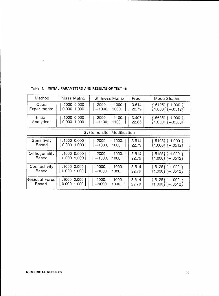
I

I

Table 3. INITIAL PARAMETERS AND RESULTS OF TEST 1bMethod Mass Matrix Stiffness Matrix Fred. Mode ShapesQuasi [.1000 0.000] 2000. -1000.] 3.514 ].5125 1.000

Experimental 0.000 1.000 -1000. 1000. 22.79 [1.000 -.0512

Initial [.1000 0.000] 2000. -1100.] 3.407 .5635[ 1.000Analytical 0.000 1.000 -1100. 1100. 22.85 1.000] -.0560

Systems after Modification

Sensitivity .1000 0.000 Ii 2000. -1000.] 3.514 .5125 1.000Based 0.000 1.000 -1000. 1000. 22.79 1.000 -.0512

Orthogonality [.1000 0.000] [ 2000. -1000. 3.514 .5125 1.000Based 0.000 1.000 -1000. 1000. 22.79 1.000 -.0512

Connectivity .1000 0.000] [ 2000. -1000.] 3.514 .5125] 1.000Based 0.000 1.000 -1000. 1000. 22.79 1.000 -.0512esidual Force .1000 0.000] Ii 2000. -1000.] 3.514 .51251.000Based0.000 1.000 -1000. 1000. 22.79 1.000 -.0512


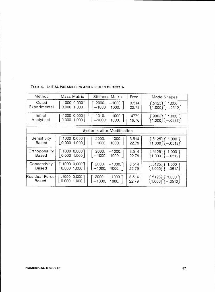
I

Table 4. INITIAL PARAMETERS AND RESULTS OF TEST 1cMethod Mass Matrix Stiffness Matrix Fred. Mode ShapesQuasi [.1000 0.000:I 2000. -1000.] 3.514 .5125 1 1.000

Experimental 0.000 1.000 -1000. 1000. 22.79 1.000 [-.0512

lnitial [.1000 0.000] 1010. -1000.] .4779 .9903[ 1.000Analytical 0.000 1.000 -1000. 1000. 16.76 1.0001 -.0987

Systems after Modifioation

Sensitivity [.1000 0.000] I; 2000. -1000.] 3.514 {S125}1 1.000 [Based 0.000 1.000 -1000. 1000. 22.79 1.000 [-.05121

Orthogonality [.1000 0.000] ' [ 2000. -1000.] 3.514 1.5125 1.000Based 0.000 1.000 -1000. 1000. 22.79 [1.000 -.0512

Connectivity [.1000 0.000] 2000. -1000.] 3.514 .5125 1.000Based 0.000 1.000 -1000. 1000. 22.79 1.000 -.0512esidual Force [.1000 0.000] [ 2000. -1000.] 3.514 .5125 1.000Based 0.000 1.000 -1000. 1000. 22.79 1.000 -.0512


Table 5. INITIAL PARAMETERS AND RESULTS OF TEST 1dMethod Mass Matrix Stiffness Matrix Freq. Mode ShapesQuasi [.1000 0.000] 2000. -1000.i| 3.514 ].51251{1.000Experimental0.000 1.000 -1000. 1000. 22.79 11.000] -.0512Initial Ii.1000 0.000] I: 110. -100.] .4161 .9161 1.000

Analytical 0.000 1.000 -100. 100. 5.494 1.000 -.0916


Seneitivity .1000 0.000 2000. -1000. 3.514 .5125 1.000Based 0.000 1.000 -1000. 1000. 22.79 1.000 -.0512Orthogonality [.1000 0.000] [ 2000. -1000.] 3.514 .51251 1.000

Based 0.000 1.000 -1000. 1000. 22.79 1.000] -.0512

Connectivity .1000 0.000jI 2000. -1000.] 3.514 .5125 1.000Based 0.000 1.000 -1000. 1000. 22.79 1.000 -.0512esidual Force [.1000 0.000] lt 2000. -1000.] 3.514 {5125 f 1.0001

Based 0.000 1.000 -1000. 1000. 22.79 1.000 1-.0512

NUNIERICAL RESULTS 68

The results of these tests indicate that the four methods work well for simple

systems. All four techniques were able to modify stiffness matrices that have minor

and/or major discrepancies with the experimental equivalents. This implies that tor

a similar problem, small errors in the determination of material properties, geometric

properties, etc., as well as large errors due to human error, can be corrected.

To examine the methods more in depth, two additional studies were considered.

First the methods were used to identify the modes of the 2 DOF system where

non-engineering changes have been made (TEST 1e and 1f). This implies that both

the initial analytical mass and stiffness matrices differ from the quasi-experimental

matrices. Secondly, the methods were also applied to a larger 8 DOF problem

(section 6.2).

The initial analytical system for TEST 1e is defined such that all springs and

masses are decreased by 10% from the quasi-experimental matrices. This system

yields the same frequencies as the original system, however the modal vectors are

not exactly the same due to round-off error. The sensitivity method does not alter the

initial analytical matrices as the quasi-experimental frequencies are properly

represented. The other three methods make minimal changes to the system

matrices as the frequencies are correct and the modal vectors are accurate to within

1%. ln other words, modal data from this system is not unique, which indicates all

systems may not be identifiable. For these results, reference Table 6 on page 70.

For TEST 1f, the initial system is defined where such that errors are present for

all of the springs and masses. The sensitivity method attempts to decrease both

frequencies by increasing the terms ofthe stiffness matrix. The orthogonality method

makes inappropriate, but minor changes to the mass matrix and also adds stiffness

to all the components the stiffness matrix. The connectivity method never changes

the mass matrix and changes the stiffness matrix to represent the system as well as


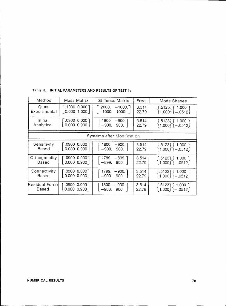
Table 6. lNlTlAL PARAMETERS AND RESULTS OF TEST 1eMethod Mass Matrix Stiffness Matrix Freq. Mode ShapesQuasi [.1000 0.000] 2000. -1000. 3.514 .5125 1.000

Experimental 0.000 1.000 -1000. 1000. 22.79 1.000 -.0512

initial [.0900 0.000] [1800. -900.] 3.514 .5123 1.000Analytical 0.000 0.900 -900. 900. 22.79 1.000 -.0512


Sensitivity [.0900 0.000] [1800. -900.] 3.514 .51231 1.000Based 0.000 0.900 -900. 900. 22.79 1.0001 -.0512

Orthogonality .0900 0.000 1799. -899. 3.514 .5123 1.000Based 0.000 0.900 -899. 900. 22.79 1.000 -.0512Connectivity .0900 0.000 1799. -900. 3.514 .5123 1.000Based 0.000 0.900 -900. 900. 22.79 1.000 -.0512esidual Force .0900 0.000 [1800. -900. 3.514 .5123 1.000Based 0.000 0.900 -900. 900. 22.79 1.000 -.0512


possible. The ratio of the components of the mass and stiffness matrices for the Equasi—experimental and updated matrices are similar. The same is true for the

residual force method. These results can be seen in Table 7 on page 72. The last

three methods are able to better represent the modal data ofthe original system, but

none are able to duplicate the original system matrices.

From these first six tests, it appears that all of the methods work well for

engineering problems. When more difficult problems exist, such as changes in the

mass matrix, then these methods generate a system which yields more accurate

modal data. However, these systems do not necessarily represent the true structure,

since the modal data is not unique.

When performing the identifications in this section, the experimental data has

been assu med to be exact. When errors exist, these methods will most likely attempt

to modify the matrices so that they generate modal data with error in it. This

indicates the need for experimental data that is accurate.

NurviERicAi. REsui:rs 71

‘ 1

Table 7. INITIAL PARAMETERS AND RESULTS OF TEST 1fMethod Mass Matrix Stiffness Matrix Freq. Mode ShapesQuasi li.1000 0.000] 2000. -1000.:] 3.514 {.5125 1 1.000

Experimental 0.000 1.000 -1000. 1000. 22.79 1.000 [-.0512

Initial [.0900 0.000] I: 2000. -1100.] 3.334 .5161 1.000Analytical 0.000 1.100 -1100. 1100. 24.02 1.000 -.0459


Sensitivity [.0901 0.000] 2101. -1201.] 3.540 .5840[ 1.000Based 0.000 1.101 -1201. 1201. 24.66 1.0001 -.0521

Orthogonality .0911 0.010] 1810. -900. 3.514 .5125 1.000Based 0.010 1.090 -900. 995. 22.79 1.000 -.0516Connectivity .0900 0.000] 1799. -1081.] 3.171 .5231 1.000Based 0.000 1.100 -1081. 1100. 22.84 1.000 -.0502esidual Force [.1000 0.000] I; 2200. -1100.] 3.514 .5125 1.000}Based 0.000 1.000 -1100. 1100. 22.79 1.000 -.0512


l

6.2 Modification Studies using an 8 DOF Model

The first study helped establish the validity of the methods. lt also indicated

sh0rt—comings of the different methods. This section will yield the results for a largerproblem which has been used in the literature (Kabe, 1985). (ref Figure 2 on page

74) (The figure is an enlarged copy from Kabe’s 1985 paper.)

The problem developed by Kabe consists of 8 degrees of freedom and 14 load

paths. It may be easiest to think of this problem as 8 masses lined up in series with

springs connecting different masses, such that the system can move only axially.The springs range in magnitude of 1.5 to 1000., and the Iumped masses range from

.001 to 1.0. There are six unique spring constants and three possible Iumped mass

values. As the entire system is grounded there are no rigid body modes. The mass

and stiffness matrices are 8 by 8 in dimension and there are 8 unique frequencies and

corresponding modal vectors associated with the system. The frequencies range

from 4.88 hz to 6.67 hz.

The original eigendata is used as the experimental data for the identification

processes. For the perturbed matrices, spring constant 1 is changed to 1050 from1000 and spring constant 6 is changed to 4 from 2. Figures 3 thru 6 contain

3-Dimensional plots which indicate the absolute value of the percent error of the

frequency prediction after applying each method. Each mode number is plotted along

the Frequency Number axis and the number of modes used in the identification

process is plotted along the Number of Modes axis. What each plot indicates is the

error in the frequency which the updated matrices yield for each set of modes used

in the identification process. By plotting in this manner, the graphs indicate what

happens to all of the modes of the system even if they are not all used in the

NuMERicAL REsuLTs 73

1

kkl P As

k § kiKS 4 6

K2K4 gsms ms mr

äK]

éK3 g K1

kl · 1(HJ kl · III) A

gz . 10 gs . l_g ·’\/‘\/‘-/L LOAD PATH

K3 · 9(D K6 · 2,0 DEGREE-CPFREDOM iml · 0.ml ms · 0.II12mj · 1.0 [ · 2, 7

Figure 2. 8 DOF TEST PROBLEM, DEVELOPED BY KABE, USED FOR SECOND EXAMPLE


lidentification process. This helps determine whether the method generates a bettersystem or just a system which represents the modal data.

Figure 3 on page 77 shows the results when using the sensitivity method. The

first set of pillars, which can be seen when viewing the graph, represent the error in

the frequency corresponding to using zero modes, or the results before any method

is applied. These errors all are less than 3% except for the last mode.

For all of the sensitivity analyses, the set of design variables chosen are donesuch that the problem will not be underconstralned. This implies that the number of

design variables is less than the number of modes used in the identification process.

Design variable linking is used between the springs, in order to modify more springs

than there are modes used. When one mode is used, all springs are linked together

as one design variable. When two modes are used, the grounded and ungrounded

links are divided into separate groups. When three, four, or five modes are used, the

springs are divided such that all springs below 5, below 250, and above 1500 are in

separate groups. For six, seven, and eight modes, all of the springs are grouped

according to the six individual stiffness values.

Examinlng the row which corresponds to the use of one mode for the sensitivity

method, it appears that the first frequency is predicted correctly. However, the

accuracy of most of the other frequencies decreases. As more modes are applied,

the accuracy of the frequencies used in the identification process increases, but the

modes not used in the identification process can become quite unrealistic.

Eventually when all 8 modes are used in the identification process, the accuracy of

all the frequencies becomes better than the corrupted finite element model. These

results for the frequencies are what would be expected; by forcing the linking of

spring constants when there are not enough measured frequencies, an exact solution

is not guaranteed. However when individual spring constants can be used, the


results are much better. Since the modal vectors are not used in the identificationprocess, the modal vectors from the updated matrices do not match the experimental

data exactly. Some terms ofthe new eigenvectors have changed both magnitude and

sign, while other terms have increased by over 25%. lnitially what these results

indicate is that the quality of any mode not used in the identification process will tend

to decrease, and that the modal vectors may not be accurately represented.

Figure 4 on page 78 is similar to Figure 3 on page 77 except that theorthogonality method ls used to update the matrices. The orthogonality method

yields correct frequencies and corresponding modal vectors for each mode used in

the identification process. lt does this at the expense of not requiring the connectivity

of the model to be the same, as well as allowing unrealistic changes to some

components of the matrices in order to generate the correct results. For this

problem, the orthogonality method correctly identifies the frequencies and mode

shapes used in the identification process, including any associated error. The other

frequencies are altered by negligible amounts.

The results of applying the connectivity method to this problem are presented in

Figure 5 on page 79. When only one mode is used in the identification process, all

of the frequencies become more accurate. The accuracy increases when two modes

are used as well. This method requires the accurate determination of the_ eigenvalues and eigenvectors of a non-positive definite matrix of rank (n x m). For

this type of matrix, l\/lSC/NASTRAN recommends using the modified Givens

eigensolution method. However, the author has found that not all of the higher

eigendata found for the matrix in this method is exact, and this can lead to some

errors in the resulting matrices. This method does perform well in correcting the

frequencies and modal vectors used in the identification while increasing the

accuracy of the other frequencies.

NUMERICAL REsuL‘rs 76

I

II

ÄPercent ErrorforSensitivity‘—Method,0H,

‘~ 4 ‘„I' 7~‘ I I „~ I'

II/l ~s ‘~ II"

r' {I 'II s~

1, ‘~IIIII*8.II, ~„

II;x —. .· A Ö7 Q}“— _, ~c>

1 ‘~,'I;'6„e

r \90 I'I' \Ü} ,' _/I/03076 .· ‘ . \S/~ 2I ‘

°

Figure 3. ERROR IN PREDICTED FREQUENCY WITH SENSITIVITY METHOD FOR 8 DOF EXAMPLE


I

Methodxl

'llI',IO‘A_ 6

\

I', ll

,,1 ,,1\\

‘~"II \\\ül'

\r \

rl. ‘\°~1 1 \ 1pl

I *~I,,'l4

6I}'I ‘~ ,1 \

"

‘«,1,,10 g)

vlI"I W ll 'I ~s~

"

lX ,· · A 87 ·' . —.l I"1

AX Sgg 5 1 • I \‘ I/' \\90 2S0 A

,’O

·' ~‘0,6 3 1O O

1

Figure 4. ERROR IN PREDICTED FREQUENCY WITH ORTHOGONALITY METHOD FOR 8 DOFEXAMPLE


ll',"~PQVCGTIIError fOf' I¤‘ I" \~„_ ,1I •COnn6·c:tivityMethod ° I

I 110 ·'

lll [I, {I,

I, ,1 •_II Xi I, lll II

·' 1 — 1' ¤. 1* ‘uI¤‘ 1

yaI'}1

R 1: Ru, 'II III 1II X • ,.\

I'.~~

~~I"

g\I"

‘\'II*‘

1 1‘„

1 1~_

2 \‘pi PX ·II xx 1/ p~1· 1· ‘p_ Q,1' R 1' * ' 1 1 1O 1 · \ 1· ¢„, 1· 1· X p_ 5 C?8 / p ,·u1¤„ 1 \ rl 1,

1I ‘¤ I \ I 1 ~‘ 1I °¤I,Pu

I,II7

iI 1¢" 1'I 1'I R

- 1' ‘\ ,· *,5 ,· Q),· \ 1 u '

‘u ’O6 Pu

1/I \" 'III

5 I \‘I I909 4 Pu

I I Ix">6S}

2 •I

1 O

Figure 5. ERROR IN PREDICTED FREQUENCY WITH CONNECTIVITY METHOD FOR 8 DOFEXAMPLE


l

Figure 6 on page 81 indicates the results of utilizing the residual force approach.The residual force vector is calculated and examined to see which springs should beused in the identification processes. The figure indicates that this method improves

the accuracy of the frequencies used in the identification process. However, thismethod is unable to consistently increase the accuracy of the modes not used in theidentification.

All of the four methods seem to be able to improve the frequencies used in the

identification process. The sensitivity method does not perform this function as well

as the others. lt tends to decrease the accuracy of the modes not used, and the

modal vectors resulting from this method also are the least accurate. The

orthogonality method yields proper frequencies and modal vectors for modes used

in the identification process, but makes minimal changes to the frequencies not used.

This method also globally modifies the stiffness matrix. V\/hen all the modes are

used, the updated stiffness matrix matches the desired analytical matrix, however

when fewer modes are used this method created terms which approached 5% ofthe

diagonal terms in the stiffness matrix. The connectivity method improves the

frequencies and modal vectors for all modes independent ot their use in theidentification process. The residual force method performed reasonable well, but themodal vectors are not as accurate as those from the orthogonality or connectivity

methods.

lt should be noted, that this example represents a complex problem, as thecomponents of the original matrices vary greatly in magnitude. The perturbations to

the stiffness matrix are also relatively large.


I&_PercentError for,’

—.ResidualForce"~

\\°’

I_

I"IO

‘~ I"I1

I' I1‘„6I, x I, xx I· \Ü I, xx

‘~ I 1 \s II1I·' ·' 6 fo

.,·’ \ ' , ,· ‘~._Ü ¢~, g)

I1 ,1, I! I1,s

~,,1 sI,’ ‘I

X III}II,03 I,

1 ’ 1 ‘x ,'I7··I1,'

"‘ Z;

'I Zbs 1r 2 .•1 G

Figure 6. ERROR IN PREDICTED FREQUENCY WITH RES. FORCE METHOD FOR 8 DOF EXAMPLE


6.3 Application of Methods with data for a free-free beam

In this section all four of the methods will be compared to actual measured

accelerometer data of a free-free beam (ref Figure 7 on page 83) (Rorrer et al, 1989).

The beam is made of steel, is 36 inches long, with a constant cross section of 1/8 in.by 1. in,. ln addition small weights were placed at 19 points along the beam. Thiswas done so that a weight could be removed and replaced by an accelerometer, and

not change the characteristics of the structure. Transverse accelerations were

determined at each of the 19 stations along the beam, and frequencies and mode

vectors were obtained for the first 6 elastic modes. The beam is supported vertically

in space by shock cords to simulate free—free boundary conditions. The experimental

modal vectors were modified by a minor shift. This was because the data was knownto contain a DC offset. The shift was determined by comparing the experimental

modal vectors with the finite element modal vectors. For an 18 element model, the

finite element results approximate Euler beam theory very well. The DC offset was

approximately 2% of twice the amplitude of the mode. Then the modal vectors were

scaled such that the triple product with the mass matrix had all ones along the

diagonal.

The original finite element model of the structure was reasonably accurate,

within 5 % for the first 6 modes. This model was obtained by utilizing 19 nodes and

18 beam elements (CBAR) (based on Euler theory with no shear stiffness) with 2-DOF

per node. In addition, 19 concentrated masses (CONl\/l2) were added to the model tosimulate the small weights. The model was reduced to match the translational

experimental data by applying Guyan reduction to eliminate the rotational DOF’s.

This operation created fully populated system matrices. l

NuiviERicAi. REsui.Ts 82

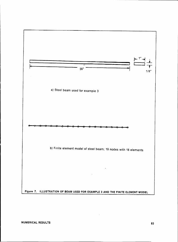
l

1Nl‘— ··lVTII TI 3B' I 1/6*

a) Steel beam used for example 3

b) Finite element model of steel beam; 19 nodes with 18 elements

Flgure 7. ILLUSTRATION OF BEAM USED FOR EXAMPLE 3 AND THE FINITE ELEMENT MODEL

83NUMERICAL RESULTS

lFigure 8 on page 85 shows the results of the identification when using the

sensitivity method. This figure is similar in format to the ones used in section 6.2.However, the scale for the percent error is smaller. For all of these identification

steps, the only design variable used is Young’s modulus. Either the mass density of

the beam or the 19 Iumped masses could have been chosen, but all would resulted

in a linear scaling of either the mass or stiffness matrix. One design variable is

chosen, as an analyst using this method would most likely assume that the propertiesof the beam were uniform throughout the length. The sensitivity method works well

for this problem. Computationally it is fairly time consuming as the change in design

variables is not accomplished in one step. However, the proper results are obtained.

This is due to the fact that the finite element model yields a satisfactory initial

solution, however perhaps too stiff. The stiffness matrix is linearly scaled down, inorder to update the matrix.

The sensitivity method requires an iterative solution. Figure 9 on page 86 showsthe convergence of the first three frequencies when applying this method to the

free—free beam example using three modes in the identification process. This methodis also dependent on the analyst, in that s/he must chose the design variables.

The orthogonality method was applied to this problem and the results are

presented in Figure 10 on page 88. This method identified all of the modes used in

the identification process, but tended to decrease the accuracy of the other modes.

lt should be noted that when two or more modes were used in the identification

process, this method generated an extraneous mode between the second and third

modes (ref Figure 11 on page 89). This mode is not recognlzable as a standard modeof a beam. For identification purposes, this mode was ignored and the proper modes

were matched to the experimental data, as the modes above the extraneous onecorrespond to the experimental mode numbers offset by one.


2

2

Error fOf' QSensitivity"€Method‘H_

I" ,1 I

4I Il,I" ~¤II3

,' ,' _2 *92 wp ,„1 ~" vl III

~dI;

‘\\~

{I O

·"‘— J,

I',Il, G

‘*X "I l1

O

Figure 8. ERROR IN FREQUENCY PREDICTION FOR BEAM USING SENSITIVITY METHOD

INUMERICAL RESULTS 85

1

1

115105

35

ZO 85

E- 75QLAJ0:6L 66>—

1.1.1 55DOELL L15

35

25

1501 2 3 L1 5 5 7 8 9 10

NUMBEB ÜF ITERFITIONSMode1 +1+ ek ak Mode2 A A A |\/|ode3 EIDE]

Figure s. couvsncsucs or= Fnsquswcuss WHEN usmc ssusmvrrv Msmon

uuMsR1cA1. Rssuus 86

1

Orthogonality

I'4

i~I,1

.· w0 I ·' f¢.,_ Ä Ä?

6 /I1 II,5

""5 ~·OÄ I," "\~~I’“6

4 ,·ll __

/1/O 3 ,· ' .@6 \Q/‘ 2Q1

Figure 10. ERROR IN FREQUENCY PREDICTION FOR BEAM USING ORTHOGONALITY METHOD


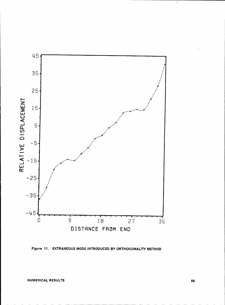
11

M5

38 /j

251-,="Z I,"Lil

1Ln.! ,·+’

Q.inO ,¤·’

>1: „·’ E< _ ’_„+—._ x_„ 1 5 _„—· “’LI-I ll

oc lf-25 /

,1- 3 5O

9 18 27 38DISTRNCE FROM END

Flgure 11. EXTRANEOUS MODE INTRODUCED BY ORTHOGONALITY METHOD

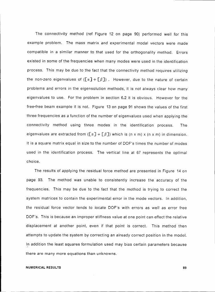
I

I

The connectivity method (ref Figure 12 on page 90) performed well for this1

example problem. The mass matrix and experimental modal vectors were made

compatible in a similar manner to that used for the orthogonality method. Errors

existed in some of the frequencies when many modes were used in the identification

process. This may be due to the fact that the connectivity method requires utilizing

the non-zero eigenvalues of (Igor] + [ß]) . However, due to the nature of certain

problems and errors in the eigensolution methods, it is not always clear how many

eigenvalues to use. For the problem in section 6.2 it is obvious. However for the

free-free beam example it is not. Figure 13 on page 91 shows the values of the first

three frequencies as a function of the number of eigenvalues used when applying the

connectivity method using three modes in the identification process. The

eigenvalues are extracted from (lim] —l- [ßj) which is (n x m) x (n x m) in dimension.

lt is a square matrix equal in size to the number of DOF’s times the number of modes

used in the identification process. The vertical line at 67 represents the optimal

choice.

The results of applying the residual force method are presented in Figure 14 on

page 93. The method was unable to consistently increase the accuracy of the

frequencies. This may be due to the fact that the method is trying to correct the

system matrices to contain the experimental error in the mode vectors. In addition,

the residual force vector tends to locate DOF’s with errors as well as error free

DOF’s. This is because an improper stiffness value at one point can effect the relative

displacement at another point, even if that point is correct. This method then

attempts to update the system by correcting an already correct position in the model.

I/n addition the least squares formulation used may bias certain parametersbecausethere

are many more equations than unknowns. I

NUMERICAL RESULTS 89 1

. I

I

1

1

11

Co n nectivItyIVI«2’t hod

," ,"I

°1 ~~‘~ I"! ~~15· I .,

,·'I \‘• 1/

2 I I, ‘~ s„

~‘rl I'

6 I"„' O

r s,x~ /,1 sx

,1 “s_I'!~s5%

36

C1

Figure 12. ERROR IN FREQUENCY PREDICTION FOR BEAM USING CONNECTIVITY METHOD

NUMERICAL RESULTS gg

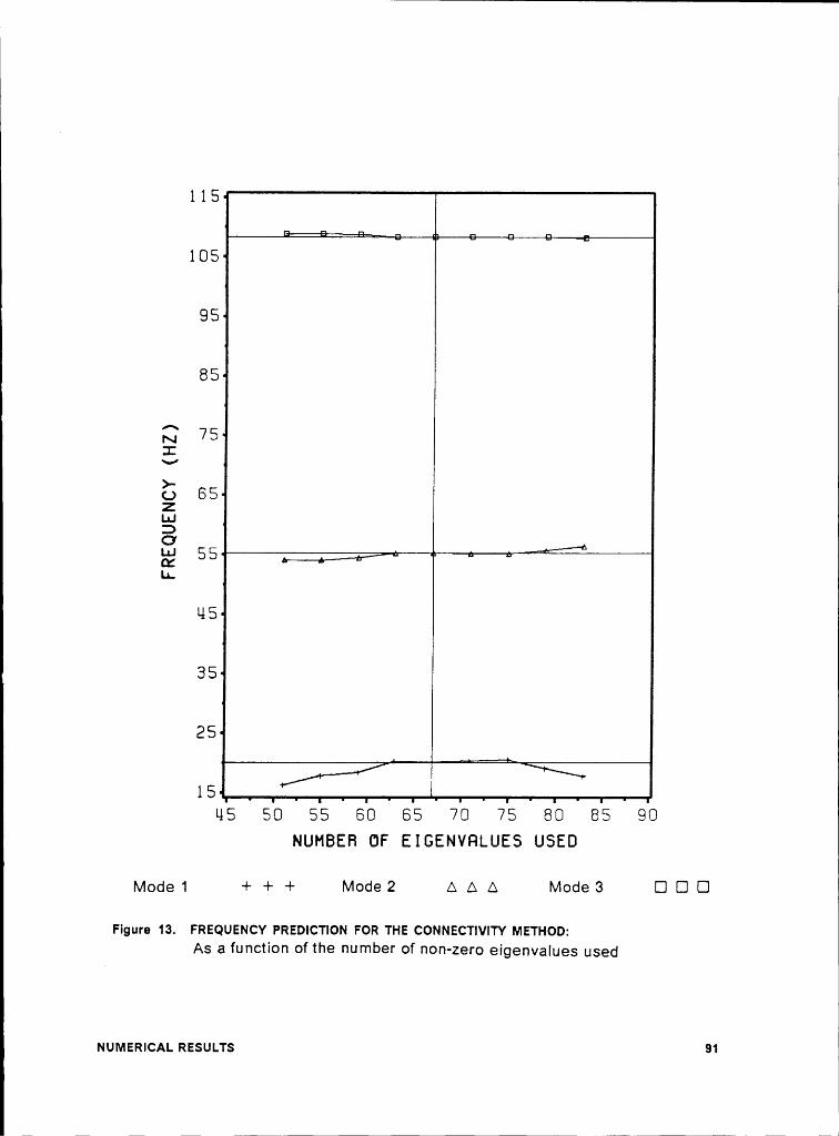
II

105

85

85

{Q 75EEE 65zLU:>O: 55 _ _ .-··-u.

L15

35

25

15L1550 55 50 55 70 75 80 85 90

NUMBEFI DF EIGENVPILUES USED

Mode1 + + + Mode2 AA A Mode3 EDI]

Figure 1s. msousucv Pmsnncriou Fon ms couuscrivrrv Msrnoo;As a function of the number of non-zero eigenvalues used

uumzmcm. Rssuus 91

The residual force method requires the analyst to determine which elements are

deficient. This is done through the use of the residual force vector, but depends on

the analyst to determine which elements to modify. Usually all of the components

of the residual force vector are not zero, so the analyst can chose all ofthe elements,

or decide what size error is negligible. This could be an automated process, but the

range of values in the residual force vector for different problems make it still

problem dependent.

Figures 15 - 20 show the first six experimentally derived elastic modes of the

free-free beam. There are six curves in each figure, and they represent modes

determined from; experimental measurements, the initial finite element model, the

sensitivity method, the orthogonality method, the connectivity method, and the

residual force method. They are the result of using six modes in the identification

process. Due to the nature of this problem we realize that the mode shapes should

resemble sine waves, hence we realize that the experimental mode shape contain

errors. The initial finite element predictions for the modes are accurate, and are only

significantly modified by the connectivity and orthogonality method.

For the first two modes the orthogonality and connectivity methods change the

mode shape. The orthogonality method matches the experimental data exactly while

the connectivity method tends to make changes opposite to the experimental results.

For the higher modes, the mode shapes from the updated matrices do not change

much from the finite element modes, except for the orthogonality method.

There are many ways to measure the effectiveness of the methods. These

include comparing the modal data from the updated system to the experimental

modal data. Another method is to examine the relative changes to the components

of the stiffness matrices. The greater the number of large percentage change, the

more an analyst will need to examine the physics of the resulting matrices. The

NUMERlcAL RESULTS 92

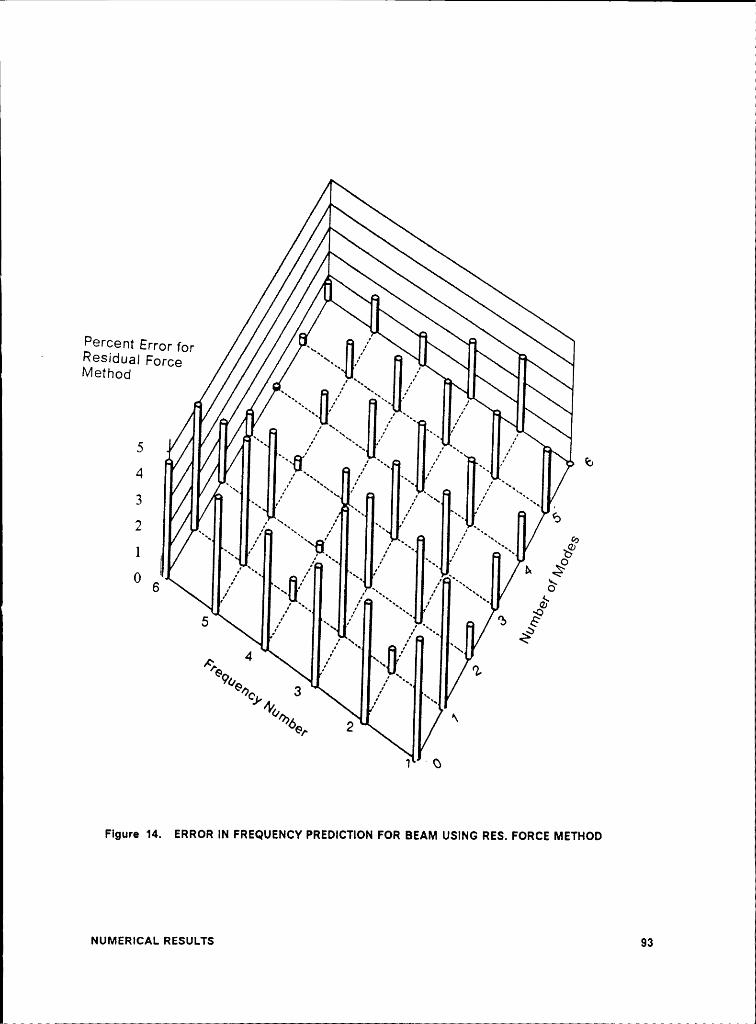
II

‘ RGSICIUGIFgrggMethod I__

:1 ~_

~~ I" ,1

~~ Ip,I3

II I, q—~

Ill] \\ ‘~~~1

‘—I/I • ~‘

I~—

~~6

I"! I'! §~II7 ,_ ,7

‘I __ ,(5.·„' ‘~. öx = ·’ ° „I1

41 ‘~,·Go

3 ·'C x‘

@6 N6, 2

1 ‘ G

Flgura 14. ERROR IN FREQUENCY PREDICTION FOR BEAM USING RES. FORCE METHOD


·1

1

111

¤ ÄÄ Y; 6

ä0<> jg

¤.EQ cu1-/ ( 1;;,2 Q E

/ / 1~ . (9m C U) W CD. ¤> CD “ cu' (DCI

E=‘“

ä‘ ¤ E „2 p- E=;:: w ‘ Ü U-ä CEEsz >„ NE

·•-· C.-->=| ...‘; (g<-> Ü: Ä-ä == 3 E-1= IX! »- 2*: cuW cu C Q;‘ \ z; ¤ <> E >~<(U< L-|-z 0.„ u.1‘·—E csQ+4 Sag‘ °* + <1 ‘¤1 \1 _ , zeEE: E 2

n 2Q‘„‘ L\ LÜO §x' ß

nlEG E E Ü ÖÖ7‘" “‘ " 'T "T 'T 7

.lN3|I30V'|dSIG 3AI1V13U

LDK . (T)

\ ‘¥\\

O <> co6*: g0O <>Q)E¢'~‘

2* 0 ·—·.- ,_ c\ Q .2 0 ¤>QQ : LL ••E(ZI U) Q)cu ä E„‘ U) E zu G)6 ul :•:

gg Cnü =:LU•Üuv:.ä Ü gg

G ‘ Ü u_ *66/Q LL O _9E J ’* LU >, LU Ü:[az; *6 q)E E 2 2 E

/ < 0 2, Qcn: >L\' W °+ g EÜ °° + <¤ 3 2,"*’·“ + 6 gs— z~ ä3· v Q Q $6Q) gg (DE

~ CD 6E O ··2L.'LU O gx .9‘ ‘*

Q O Q O O3 3 3 2 W W W WJ.N3H30V'IdS|0 3AI1Y'I38

95NUMERICAL RESULTS

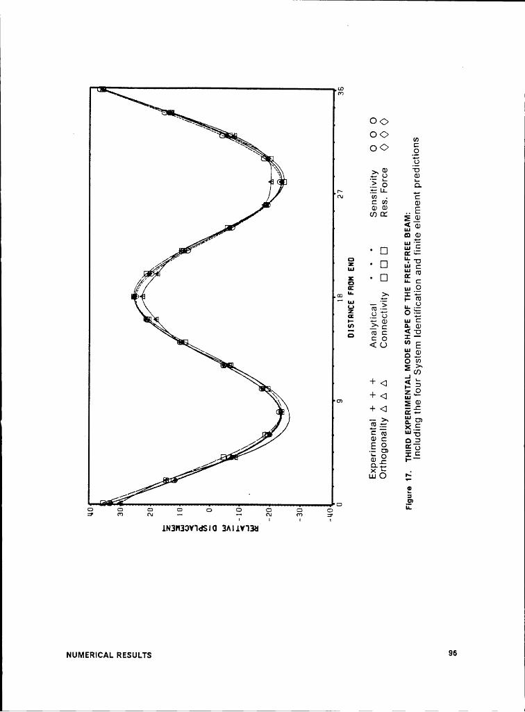
‘ I

•.' ¢¤(77

O<>‘ ose OO\\ OO Q•i-aÖ3 2=<,· E Es 21’ 1~ :*;‘U·- .,.."’ 2 ui E

.·(D G) Ewo: E9fa E Q)Z” mg,‘ WE

/ g ‘ÜZ'}:ä ’ Ü E c

fz:ES ggä'”-‘“! ¢ äg) mg‘ w 2: ¤ cuCG C (U

x., C 0gg

?‘.1+ Q < E+ <1 5*

rz + Q EE» EE EE, !a· C N ‘“‘OCD C Q3E 8 SEB5;, 2 ·ä O.C

„_..,/ O §1Q Q Q Q Q O Q Q Q u'

""’ “‘ T T ‘T‘ °7 i'

.lN3H39Y”IdSIG 3Al.I.Y”l3U

~uMsmcAL Rasuus 96

4

IX,r·“·%

4 %‘$.;'.____

. OOe. — OO U)

. c:g, OO .9‘” T5

* *¤.. 3„ E ,3 Q

. ‘ rv " E* ° 3 3 ..3E

< icewc: <.Q

ä culu

Iä·E

¤ ny;

;* " Ü Cz: '* NQ

‘ Ü u; E

f“’-> _ 1:

4 '°E°§ QQ ‘“>„‘ä’F-? ms;

L 'Q¤_ ·•-«

•- *— U C2 ‘$~ 2 § ¤>\x Q CUCII'}: gc cm

gwsg:. + <] äE

+ <1 EE- , 6 E ·“ 3*V

•·-· Z I--.

C cu •-*¤

·,.‘CD Q ßg

O— _ E O [LE

‘ ¤.·E .

3

2 2, 3 ¤ C, D O*·—‘

Q¤T'Y 'P 2

1N3|‘l30V'ldS|(I 3A|.I.V'l38

Ä

2 <><>„·= OO $2 *Ä OO .9T9

‘ ._ E E Q‘\ 2 Q ·gE · N äää E(D CI ägT'} 4 ID Q)

{SEI 25 'Ü·‘§

· I] Ü} Q/ N Ü E (U[FT:; U. E

’”ä nu O„ ¢= >_ 1 x:: I> CD uh 1:PT3 5 2 ‘ö =6 ä 2 G „„ E··· Tv C I

'Q

äU)\.·\'¤

SB9 2si ‘U)

E ·-I L-„ + 6 E gO')_

+ <1 ¤: "T~-jf->„··’ TE E ä 5C (U 3!^Y • Q) ä¤> -5C O ß,•>”°

. >< °·: cä._ LU O ··RA-ä=$r§G

G G G G G G G Ü=" ‘“ ^’ '” T °T‘ T ZT.I.N3|'|3OV”IdS|G ]A|.lV'l38

98NUMERICAL RESULTS

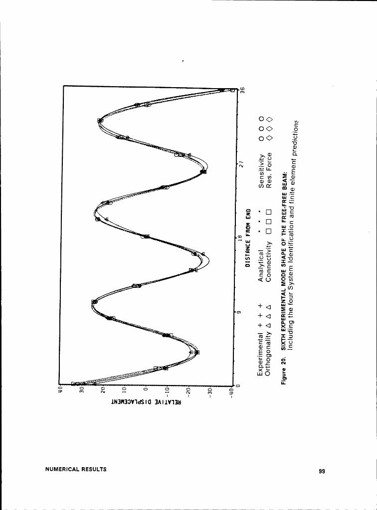
1

I

11

<>’\OO _Q

<>O>„ O Q>O1N E LL

vi E CD„·· Qi GJQ)z ·‘ w E

uf;.} I1;. _¤1; Cu.: ¤: ‘°

(Ü E e IL Cä -¤ .21 L {E ‘ Ü 1*5 *6 L•ÄÜ' (D LL OL1 E O°$ g ¤kl * •— N LZ < CDw .9 u I EQ an E<$“:

m E luc O ¤ EI,- < 0 ¤ wL

<¤ ä EU)

¤. OJ<l äg

:3 #5 I EC

zuzwiX C E’ LU Ü ä,EQ Q Q Q Q Q Q Q Q=" "’

"' ’“ 'T T T 7.|.N3l30V1d$|0 3A|1V'|]8

l

orthogonality method makes many large relative changes to the stiffness matrix. This

is because this method models the modal data exactly, including the error. The many

high percentage changes are mostly due to the modification of stiffness coefficients

with small initial values. All ofthe other methods make small changes to the stiffness

matrix components. Table 8 on page 101 shows the relative changes to the diagonal

components of the stiffness matrices for each method when analyzing the free-free

beam using six modes. Table 9 on page 102 shows the relative changes to the off

diagonal terms. Note that for the residual force method, better results were obtained

by modifying the concentrated masses only, therefore there are only 19 terms which

can be changed instead of the 361 terms in the full matrix.

The computational times are also of interest to an analyst when considering the

usefulness of a method. Table 10 on page 104 shows the CPU time on a l\/licro·VAX

ll computer for each method when utilizing 1 thru 6 modes. These times can be

compared to a time of 2:09 for the analysis of the finite element model only. All

methods performed the finite element calculations, so the the modification time is the

differential between 2:09 and the time listed. The time used by the orthogonality

method is consistently lower than the other methods and the time is only slightly

dependent on the number of modes used. The connectivity method is the most

expensive to use for each set of modes used. This may be due to the fact that there

is quite a bit of looping done for this method, and the way this was programmed with

the DMAP language in MSC/NASTRAN may not be the most efficient method. The

sensitivity method is highly dependent on the number of modes in the identification

process, even though the same stiffness matrices are generated. The residual force

method does not seem highly dependent on the number of modes used, this may be

due to the fact that the method is programmed to generate the column vector

associated with each element.


Table 8. RELATIVE CHANGES TO MATRICES, # OF DIAGONAL TERMS CHANGED

METHOD #< 1% #< 10% #< 100 #>100%99991111111 Xi 19 1111ORTHOGONALIW 9 17 1iÄ;@@9999111111 9 14 1ll$1199191191 FORCE 13I

NUMERICAL RESULTS 101I

_ _ _ _ _

Table 9. RELATIVE CHANGES TO MATRICES, # OF OFF-DIAGONAL TERMS CHANGED

METHOD #< 1% #< 10% #< 100 #> 100%SENS'T‘V'W K1 342 §§K$ORTHOGONAUTY jlli 74 2666¤~~66T~¤¤ 266 16666666 66666 §$l§i$1l

Table 10. CPU TIME REQUIRED FOR THE FOUR METHODS FOR FREE-FREE BEAM (minzsec)

METHOD 1 MODE 2 MODES 3 MODES 4 MODES 5 MODES 6 MODESSENSITIVITY 4:12 6:12 10:52 12:45 14:43 17:10

ORTHOGONALITY 2:27 2:23 2:24 2:25 2:24 2:36CONNECTIVITY 12:53 13:54 14:57 16:30 18:40 21:17

RESIDUAL FORCE 7:46 7:49 7:53 7:56 8:00 8:15


l

It is interesting to note the results from some of the methods change with small

changes in the experimental data. The sensitivity method works independent oferrors in the modal matrix, and it is dependent only on the frequencies. The

orthogonality method models the experimental data very well, but the resultingupdated system matrices can change for even small changes in the modal data. The

connectivity method does not seem to be affected as much by changes in the modal

data. The residual force method seems to be the most sensitive to changes in the

modal data. This gives another indication of the difficulty in obtaining quality results.

lt is beneficial for the connectivity method in that it is less sensitive to errors in the

experimental data.


Chapter VII

CONCLUSIONS AND RECOIVINIENDATIONS

7.1 Conclusions

This thesis reviewed many System Identification methods, and examined four

methods in depth. All of the four methods appeared to be able to update analytical

system matrices using modal data. However not all of them performed the

identification as well as desired. They all exhibited pros and cons.

The sensitivity method was able to adequately modify the system matrices in

order to generate an accurate match for the modes used in the identification process.

However, modes not used were generally not improved, and the modal vectors from

the updated model were not as accurate as the second and third methods.

However this method worked quite well for the free-free beam example. There

were no large errors in the analytical model and this method could then scale the

stiffness matrix to get a better representation of the frequencies. The resulting mode

coNcl.usloNs AND REcoMMENDATloNs 105

l

shapes did not fit the experimental data exactly, which may be beneficial as all

experimental data contains errors. Since this method performs element by element

changes only, it retains the connectivity of the original model. The iterative nature

of this method means that it is computationally expensive.

The orthogonality method was able to update the frequencies and mode shapes

used in the identification process for the second example problem. However, it did

not improve the accuracy of the modes that were not used. Similar results were

obtained for the free-free beam. However, a new mode was introduced to the system,

and large relative changes were made to the system matrices. This indicates that

there must be high confidence in the experimental data for this method to be used.

This method does not preserve the original connectivity of the model and results in

a less physically meaningful model. The connectivity criteria is not important for a

model which has been reduced to fewer degrees of freedom. However, this method

is the least expensive to use and the updated matrices model the modal data used

in the identification process very well.

The connectivity method did an excellent job of updating the modes for the 8 DOF

example. lt was able to improve the accuracy of modes that were not used in the

identification. This is beneficial and indicates that the resulting matrices are likely to

be correct. This method performed well for the third example. This method requires

the accurate determination of all of the eigenvalues and eigenvectors of a large

non-positive definite matrix. The recommended solution technique is the modified

Givens, and the accuracy of higher eigenvalues may not be good. However, this

method does retain the original connectivity of the model. This method is fairly

computationally expensive to use, but makes minimal changes to the stiffness matrix.

The residual force method worked well for the second example. lt was able to

improve the accuracy of all modes in the identification process as well as modes that

CONCLUSIONS AND RECOMMENDATIONS 106

l

were not included. This method did not work as well for the free—free beam example.

This may be due to the difficulty of locating only the DOF’s with errors within the

model. The technique of solving for new variable values can result in a highly over

constrained problem which may bias certain variables. This method does preservethe connectivity of the original model, and is not the most computationally expensivemethod to use.

The following is a list of the methods and when they are beneficial, in order of

preference by the author. The connectivity method works well for many models, and

the derivation lends itself to give the analyst confidence in the resulting model. The

residual force method has great potential, and might improve ifa better error location

technique were developed, and if [Q] could be reduced to be square by another

means than a least squares fit. The orthogonality method requires very accurate

modal data to yield physically meaningful system matrices. The sensitivity method

works very well for problems where the analyst realizes that the model is physically

correct, but there may be errors in only a few variables (for example, material

properties).

7.2 Recommendations

Structural analysis techniques have developed to the point where confidence can

be placed on their results. There will be minor errors though, and they should be

corrected. But, any resulting modification is only as good as the experimental data

that ls used. And this data will contain errors. Therefore, a method which allows for }a standard deviation in the experimental data, or a confidence level in the analytical

}c0NcLus|oNs AND REcolvlMEN¤A‘rloNs 107

i

and experimental data would be beneficlal. This could be accomplished by utilizing

a Bayesian technique (B|akely and Walton, 1984).

Perhaps a combination of some of these methods would yield a better System

Identification method. First, it would be beneficlal to be able to have the mass matrix

where the modal vectors are orthogonal. This could be done by using the technique

utilized in the orthogonality method. Perhaps a better method would be to modify the

modal vectors as well as the mass matrix, as there is probably a higher confldence

level in the mass matrix than there is in the modal vectors. The confldence in

frequencies is usually good, so the experimental frequencies should not be modified.

Different variation of these techniques were presented by Targoff (1976) and Baruch

(1982).

Once the mass matrix and modal vectors are compatible, then perhaps a

sensitivity method should be used to improve the stiffness matrix. This should not

necessarily be done on an element by element basis, but instead by linking elements

in the model that are similar; i.e. elements in similar geometric regions with the sameÄ

material properties. Once global changes are made to update the matrices, while

retaining the connectivity, then element by element changes could be made. For an

analytical model which has not been reduced, the connectivity method could be used

to perform the final model modification. Or, if a better error location technique is

developed, then the residual force technique could be used as well. lf the model is

reduced then the orthogonality means of updating could be used.

It should be noted that the orthogonality and connectivity methods are similar for

a reduced model (fully populated matrices). However, the orthogonality method uses

a mass weighted objective function in the optimization process. The connectivity

minimizes the un-weighted percent change to the stiffness coefficients. lf an analyst


1

has intuitive knowledge of the problem to be solved, s/he may prefer one methodover the other.

This resulting method would utilize many ofthe benefits ofthe four methods. The

resulting model should contain minimum changes to the system matrices whileyielding good predictions of the modal data.


Chapter Vlll

Barthelemy, B., and Haftka, R. T., "Physically Based Sensitivity Derivatives for FiniteElement Programs," Proceedings of A/AA/ASME 28th Structures, StructuralDynamics, and Materials Conference, April 1987, pp. 642 - 650

Baruch, M., and ltzhack, "Optimal V1/eighted Orthogonalization of Measured Modes,"AIAA Journal, Vol. 16, No. 4, April 1978, pp. 346 - 351

Baruch, M., "Optimization procedure to Correct Stiffness and Flexibility Matricesusing Vibration Tests" AIAA Journal, Vol. 16, No. 11, Nov. 1978, pp. 1208 - 1210

Baruch, M., "Methods of Reference Basis for Identification of Linear DynamicStructures," Proceedings of AIAA/ASME 23th Structures, Structural Dynamics,and Materials Conference, May 1982, pp. 557 - 563

Berman, A., and Flannely, VV. G., "The Theory of lncomplete Models of DynamicStructures," A/AA Journal, Vol. 9, No. 8, Aug. 1971, pp. 183 - 192

Berman, A., "Determining Structural Parameters from Dynamic Testing," Shock andVibration Digest, Vol. 7,Jan. 1975 pp. 10-17

REFERENCES 110

Berman, A., "Parameter Identification techniques for Vibrating Structures," Shock andVibration Digest, Vol. 11, Jan 1979, pp. 13 - 16

Berman, A., "Mass Matrix Correction Using an Incomplete Set of Measured Modes,"AIAA Journal, Vol. 17, No. , 1979, pp. 1147 - 1148

Berman, A., and Nagy, E. G., "Improvement of a Large Analytical Model Using TestData," AIAA Journal, Vol. 21, No.8, Aug. 1983, pp. 1168 — 1173

Blakely, K. D., and Walton, W. B., "Selection of Measurement and ParameterUncertainties for Finite Element Model Revision," 2nd lMAC, Orlando Florida,1983, pp. 82 - 86

Caesar, B., "Updating System Matrices using Modal Test Data," 5th lMAC, OrlandoFlorida, 1986, DD. 453 — 459

Chen, J. C., and Garba, J. A., "Ana|ytical Model Improvement Using Modal TestResuIts," AIAA Journal, Vol. 18, No. 6, June 1980, pp. 684 - 690

Chen, J. C., and Wada, B. K., "Matrix Perturbation for Structural Dynamic Analysis,"Proceedings of AIAA/ASME 29th Structures, Structural Dynamics, and MaterialsConference, April 1988, pp. 355 - 364

Chen, T. Y., and Wang, B. P., "Finlte Element Model Refinement Using Modal AnalysisData," Proceedings of AlAAlASME 29th Structures, Structural Dynamics, andMaterials Conference, April 1988, pp. 1219 - 1229

Collins, J. D., Hart, G. C., Hasselman, T. K., and Kennedy, B., "StatisticaI Identificationof Structures," AIAA Journal, Vol. 12, No. 2, Feb. 1974, pp. 187 - 190

Dobson, B. J., "Modification of Finite Element Models using Experimental ModalAnalysis," 2nd lMAC, Orlando Florida, 1983, pp. 593 - 597

Fuh, J., Gustavson, B., and Berman, A., "Error Estimation and Compensation inReduced Dynamic Models of Large Space Structures," Proceedings ofAlAAlASME 27th Structures, Structural Dynamics, and Materials Conference,April 1986, DD- 1 - 9

I-laftka, R. T., and Kamat, M. P., Elements ofStructura/ Optimization, Martinus NijhoffPublishers, Boston, 1985

REFERENCES 111

Guyan, R. J., "Reduction of Stiffness and Mass Matrices," AIAA Journal, Feb. 1965,Vol. 3, No. 2, p. 380

Hall, B. M., Calkin, E. D., Sholar, M. S., "Linear Estimation of Structural Parametersfrom Dynamic Test Data," Proceedings of AlAAlASME 77th Structures, StructuralDynamics, and Materials Conference, April 1970, pp. 193 — 197

Haug, E. J., Komkov, V., Choi, K. K., "Design Sensitivity Analysis of StructuralSystems/’ Academic Press, 1984

Heylan, W., and Sas, P., "Review of Model Optimization Techniques," 5th lll/IAC,Orlando Florida, 1986, pp. 1177 - 1182

Ibrahim, S. R., and Saafan, A. A., "Correlation of Analysis and Test in Modeling ofStructures Assessment and Review,” 5th /ll/IAC, Orlando Florida, 1986, pp. 1651— 1660

Jain, V. K., and Dobeck, G. J., "System Identification Techniques: a TutorialReview," in 79-WA/DSC-20, ASME, New York, 1979

Kabe, A. K., "Stiffness Matrix Adjustment Using Mode Data," A/AA Journal, Vol. 23,No. 9, September 1985b, pp. 1431 - 1436

Kidder, R. L., "Reduction of Structural Frequency Equations," A/AA Journal, Vol. 11,No. 2, Feb. 1973, p. 380

Lancaster-Brown, Peter, "Halley & His Comet," Blanford Press, New York, NY, 1985

Luk, Y. W., "ldentification of Physical Mass, Stiffness and Damping Matrices UsingPsuedo-lnverse," 5th IMAC, Orlando Florida, 1986, pp. 679 - 685

Macneal-Schwendler Corporation, "User Manuals. Vol 1 and 2," Los Angeles, CA,July, 1984

Nelson, R. B., "Simplified Calculation of Eigenvector Derivatives/’ AIAA Journal, Vol.14, 1976, p. 1201-1205

REFERENCES 112

l

i

O’Cal|ahan, J. C., Avitabile, P., and Leung, R., "Deve|opment of Mass and StiffnessMatrices for an Analytical Model using Experimental Data," 2nd IMAC, OrlandoFlorida, 1983, pp. 585 — 592

O’Cal|ahan, J. C. and Leung, R. K., "Optimization of Mass and Stiffness Matricesusing a Generalized lnverse Technique on Measured Modes," 3rd IMAC, OrlandoFlorida, 1984, pp. 75 - 79

Ojalvo, l. U., and Pilon, D., "Diagnostics for Geometrically Locating Structural MathModel Errors from Modal Test Data," Proceedings of AIAA/ASME 29th Structures,Structural Dynamics, and Materials Conference, April 1988, pp. 1174 - 1186

Pakstys, M. P., "Correlation of Experimental and Analytical Structural DynamicsParameters - A 1982 Overview," 1st IMAC, Orlando Florida, 1982, pp. 59 - 63

Pal, T. G., and Scmidtberg, R. A., "Combining Analytical and Experimental ModalAnalysis for Effective Structural Dynamic Modelling," 1st IMAC, Orlando Florida,1982, pp. 265 - 271

Rorrer, R. A. L., Wicks, A. L., and Williams, J., "Angular Acceleration Measurementsof a Free-Free Beam," To be presented at the 8th IMAC, 1989

Shye, K., and Richardson, M., "Mass, Stiffness, and Damping Estimates fromStructural Measurements," 5th IMAC, Orlando Florida, 1986, pp. 756 - 761

Sidhu, J., and Ewins, D. J., "Correlation of Finite Element and Modal Test Studies ofa Practical Structure," 2nd IMAC, Orlando Florida, 1983, pp. 756 - 762

Sol, E., Verdonck, E., Snoeys, R., and Wilde, W. P., "Design Optimalisation of DynamicStructures by the Combined use of Modal Analysis (M.A.) and the Finite ElementMethod (F.E.M.)," 2nd IMAC, Orlando Florida, 1983, pp. 769 — 776

Targoff, W. P., "Orthogonality Check and Correction of Measured Modes," A/AAJournal, Vol. 14, No. 2, Feb. 1976, pp. 164 - 167

Vanhonacker, P., "A Methodology for Combining Experimental and MathematicalModal Analysis with Application to an Automotive Component," 5th IMAC,Orlando Florida, 1986, pp. 406 - 408

REFERENCES 113

ll

l

Wang, B. P., and Chu, F. H., "Effective Dynamic Reanalysis of Large Structures,"Shock and Vibration Bu//etin, No. 51, May 1981, pp. 73 - 79

Wang, B. P., and Chen, T. Y., "Model Refinement using Test Data," 4th /ll/7AC, OrlandoFlorida, 1985, pp. 1052-1056

Yokoki, K., Hayakawa, S., and Yoshlno, H., "Optimization of Finite Element Modelingusing Experimental Modal Analysis and Sensitivity Analysis,“ 5th /il/IAC, OrlandoFlorida, 1986, pp.

Vllei, F. S., "Stiffnes Matrix Correction From lncomplete Test Data," A/AA Journal, Vol.18, No. 10, October 1980, pp. 1274 - 1275

Zienkiewicz, O. Z., "The Finite Element Method in Engineering Science," McGrawHill, New York, 1967

REFERENCES 114

Appendix AModeling and Solution Sequences from

MSC/NASTRAN

Summary of solution methods available in MSC/NASTRAN for the System Identificationof vibrating stuctures

The following are the MSC/NASTRAN Version (64/65) solution sequences for systemidentification methods.

115

I

A.1 Solution Sequence for Sensitivity Based MethodID MSONASTRAN $PASTIME 100$$$$ THIS METHOD USES A NEVVTON—RAPHSON ITERATIVE SCHEME TO

ä UPDATE THE SYTEM MATRICES BASED ON SENSITIVITY INFORMATION$ M is the number of measured frequencies$ R is the number of design variables$$BEGIN$$ 1.)$ INITIALIZE THE DATABASEDBMGR //0/V,Y,DBCLEAN=0/V,Y,DBNBLNKS=40000//V,Y,DBINIT=0//

V,Y,DBNAME=DB01 $$$ 2.) STORE MATRIX DERIVATIVES IN DATABASEADD MXX,/OMXXADD KXX,/OKXXDBSTORE OMXX,OKXX//1/1$ADD MXX,/DMXXJ/(0.0,0.0)ADD I<XX„/DKXXJ/(3.333E-8,0.0)DBSTORE DKXXJ,DMXXJ//1/1ADD MXX,/DMXXJ/(1365.0,0.0)ADD KXX,/DKXXJ/(0.0,0.0)DBSTORE DKXXJ,DMXXJ//2/1$$ 3.) INITIALIZE AND RENAME MATRICESADD KXX,/KAADD MXX,/MADBSTORE KXX.MXX,KA,MA// $FILE SENSCT=APPENDFILE SENSM=APPENDFILE AAT=APPENDFILE BBT=APPENDMATMOD VI/V,,,,,/VI/M,/28DIAGONAL WM/VEC1/C,Y,SQUARE/V,Y,POWER =0.$ .PARAM //NOP/V,Y,KLOOP=0$PARAM //ADD/V,Y,KLOOP1/V,Y,MM=0/1PARAM //ADD/V,Y,KLOOP2/V,Y,RR=0/1PARAM //ADD/\/,Y,KLOOP3/V,Y,MM=0/1PARAM //ADD/V,Y,MMM1/V,Y,MM=0/-1PARAM //ADD/\/,Y,MMP1/V,Y,MM=0/1PARAM //ADD/\/,Y,RRP1/V,Y,RR=0/1PARAM //SUB/V,Y,NMM/0/V,Y,MM=0PARAM //SUB/V,Y,NRR/0/V,Y,RR=0PARAMR //NOP/\/,Y,FOLD=10000.$

116

I

I

$ 4.) TOP OF ITERATIVE LOOPLABEL TOPLOOP

PARAM //ADD/V,Y,KLOOP/V,Y,KLOOP/1PRTPARM //0/C,N,TOPLOOP$

$ 5.) PERFORM EIGENVALUE ANALYSISDBFETCH /KA,MA,,,/ $SETVAL //\/,N,NE|GVS/-1 $READ KA,MA,,,DYNAM|CS,,CASECC/LAMA,P|··|IX„MI,OElGS/ V,N,

READAPP=MODES/S,N,NEIGVS $OFP LAMA,OE|GS// $

$$ 6.) GENERATE ANALYTICAL AND EXPERIMENTAL FREQUENCIES

PRTPARM //0/C,N,FREC)GENLAMX ,,LAMA/LAMM1/-1PARTN LAMM1,,LPV/JUNK,LAMM,,/1ADD LAMM,/NLAMM/-1.MATMOD LAMM,,,,,/AF,/1/3MATMOD NLAMM,,,,,/NLAMBDA,/1/1TRNSP AF/AFTTRNSP NLAMBDA/NLAMBDATADD AF,EF/DELFREC)//-1.TRNSP DELFREO/DELFREQT

$$ 7.) EXIT LOOP IF ERROR IS SMALL OR DOES NOT DECREASE

PRTPARM //0/C,N,JUMPSHIPMPYAD DELFREOTDELFREC),/FPARAML F//DMI/1/1/V,N,FPRTPARM //0/C,N,FPARAMR //LE//F/1.E—6////V,N,FLAGCOND OUTLOOP,FLAGPARAMR //SUB/V,N,FOMFN/FOLD/FPRTPARM //0/C,N,FOLDPRTPARM //0/C,N,FOMFNPARAMR //LE//FOMFN/1.E-3////V,N,FLAGCOND OUTLOOP,FLAGPARAMR //ADD/V,N,FOLD/F/0.

$$ 8.) LOOP TO STORE ANALYTICAL DATA

PRTPARM //0/C,N,STOREPARAM //ADD/V,Y,KLOOP1/V,Y,KLOOP1/NMM $ # CORRESPONDS TO (-M) CHANGELABEL KTOP1

PRTPARM //0/C,N,KLOOP1MATMOD PHIX,,,,,/UI,/1/KLOOP1DBSTORE UI//KLOOP1/1PARAM //ADD/V,Y,KLOOP1/V,Y,KLOOP1/1PARAM //SUB/V,N,FLAG/V,Y,MM/V,Y,KLOOP1COND OUT1,FLAG

REPT KTOP1,1000 $ # CORRESPONDS TO (M-1). CHANGELABEL OUT1

$$ 9.) DETERMINE SENSITIVITY OF FREQUENCIES W/RESPECT TO DESIGN VARIABLES

PARAMR //ADDC////V,Y,MPYR/(.012665,00)$PURGE SENSM/NEVERPARAM //ADD/V,Y,KLOOP2/V,Y,KLOOP2/NRR $ (-R) CHANGELABEL KTOP2

117

I

II I

PRTPARM //0/C,N,KLOOP2DBFETCH /DMXXJ,DKXXJ,,,/KLOOP2/1PURGE SENSCT/NE\/ERPARAM //ADD/V,Y,KLOOP3/V,Y,KLOOP3/NMM $ # (-M) CHANGELABEL KTOP3

PRTPARM //0/C,N,KLOOP3MATMOD PHIX,,,,,/UI,/1/KLOOP3TRNSP UI/UITSCALAR NLAMM//KLOOP3/1/S,Y,NLISCALAR LAMM//KLOOP3/3/S,Y,FIADD DKXXJ,DMXXJ/DXX//NLISMPYAD UIT,DXX,U|,,,/DLIDXJ/3PARAMR //DIVC////V,Y,MFI/V,Y,MPYR/V,Y,FI/V,N,FLAGADD DLIDXJ,/DFIDXJ/MFIAPPEND DFIDXJ,/SENSCT/2 BDBSTORE DFIDXJ//KLOOP2/KLOOP3PARAM //ADD/V,Y,KLOOP3/V,Y,KLOOP3/1

PARAM //SUB/\/,N,FLAG/V,Y,MM/V,Y,KLOOP3COND OUT3,FLAGREPT KTOP3,1000 $ # CORRESPONDS TO (M-1). CHANGELABEL OUT3TRNSP SENSCT/SENSCAPPEND SENSC,/SENSM/2PURGE SENSCT/ALVVAYSPARAM //ADD/V,Y,KLOOP2/V,Y,KLOOP2/1PARAM //SUB/V,N,FLAG/V,Y,RR/V,Y,KLOOF’2COND OUT2,FLAG

REPT KTOP2,1000 $ # CORRESPONDS TO (R-1). CHANGELABEL OUT2

$$ 10.) CREATE SOUARE MATRIX

PURGE AAT.BBT/NEVERTRNSP SENSM/AATPURGE SENSM/ALVVAYSTRNSP DELFREO/BBTTRNSP AAT/AATRNSP BBT/BBFILE NAA=APPENDFILE NBB=APF’ENDPURGE NAA,NBB/NEVERPARAM //NOP/\/,Y,KLOOP4=1LABEL KTOP4

PRTPARM //0/C,N,KLOOF’4SCALAR LAMM//KLOOP4/3/S,Y,FIMATMOD DELFREQT,,,,,/DELF,/1/KLOOP4PARAMR //D|VC////\/,Y,ONEOF/(1.0,0.0)/V,Y,FI/V,N,FLAGADD DELF,/NDELF/ONEOFAPPEND NDELF,/NBB/2MATMOD AAT,,,,,/D1,/1/KLOOP4ADD D1,/ND1/ONEOFAPPEND ND1,/NAA/2MATPRN NAA,NBB//$PARAM //ADD/V,Y,KLOOP4/V,Y,KLOOP4/1PARAM //SUB/V,N,FLAG/V,Y,MM/V,Y,KLOOP4COND OUT4,FLAG

REPT KTOP4,1000 $

118

LABEL OUT4PARAM //SUB/V,Y,KLOOP4/V,Y,KLOOP4/MMTRNSP NAA/AATRNSP NBB/BBPURGE NAA,NBB/ALWAYSTRNSP AA/AATMPYAD AAT,AA/ATA$MPYAD AAT,BB/ATB

$ 11.) SOLVE SYSTEM OF EQUATIONSSOLVE ATA,ATB/NXXADD NXX./XX/(-3.0,0.0)PURGE AAT,BBT/ALWAYS

$$ 12.) EXTRACT COMPONENTS OF XX (DELTA X) VECTOR

MATPRN XX// $SCALAR XX//1/1/S,Y,X1

S$ 13.) ASSEMBLE NEW MASS AND STIFFNESS MATRICES

DBFETCH /KXX,MXX,,,/ $DBFETCH /DKXXJ,,,,/1/1ADD DKXXJ,/KADD1/(3.333E-3,0.0)ADD KXX,KADD1/KA//X1ADD KA,/KXXADD MA./MXXDBSTORE KXX,MXX,KA,MA// $PARAM //SUB/V,N,FLAG/V,Y,NITER/V,Y,KLOOPCOND OUT,FLAG

$ 14.) REPEAT ITERATIVE LOOP 5 TIMESREPT TOPLOOP,1000LABEL OUT$$ JUMP HERE IF ERROR IS SMALLLABEL OUTLOOPPRTPARM //O/C,N,JUMPEDSHIP$$ PRINT RESULTSPRTPARM //0/C,N,RESULTSMATPRN KA,MA// $MATPRN EPHI,PHIX// $$$DBFETCH /OMXX,OKXX,,,/1/1$DBFETCH /KA,MA,,,/ $ADD OMXX,MA/MDIF//-1.ADD OMXX,MDIF/MPERC///2ADD OKXX,KA/KDIF//-1.ADD KDIF,OKXX/KPERC///2MATPRN MPERC,KPERC// $MATPCH PHIX// $$$ END PROGRAMEND$CEND$

119 I

I

I

$ INFORMATION PERTINENT TO ANALYSISMETHOD=10DISPLACEMENT = ALLSPC=1MODES=3$$ ENTER PHYSICAL DATA BELOVVBEGINBULK8PARAM , NITER , 30PARAM,MM,6F°ARAM,RR,1$DM|,LPV,0,2,1,0,,8,1DMI,LPV,1,3,1.,THRU,8$DMI,EQ1,0,2,1,0,,4,1DM|,EO1,1,1,0.000111111,0.,1.,0.DMI,EQ2,0,2,1,0,,4,1DMI,EQ2,1,1,0.,.0011111,0.,1.$ $DMI,R1,0,2,1,0,,1,1DMI,R1,1,1,0.DM|,R2,0,2,1,0,,1,1DMI,R2,1,1,0.$$DMI,KXX,0,2,1,0,,2,2$DMI,KXX,1,1,1900.,-900.$DMI,KXX,2,1,-900., 900.$DMI,MXX,0,2,1,0,,2,2$DMI,MXX,1,1,.1$DMI,MXX,2,2,1.$DMI,DKXX1,0,2,1,0,,2,2DMI,DKXX2,0,2,1,0,,2,2DMI,DKXX3,0,2,1,0,,2,2DMI,DKXX4,0,2,1,0,,2,2DMI,DMXX1,0,2,1,0,,2,2DMI,DMXX2,0,2,1,0,,2,2DMI,DMXX3,0,2,1,0,,2,2DMI,DMXX4,0,2,1,0,,2,2DMI,DKXX1,1,1,1.DMI,DKXX2,1,1,1.,-1.DMI,DKXX2,2,1,-1.,1.DMI,DMXX3,1,1,1.DMI,DM><><4,2,2,1.$5DMI, WV,0,2,1,0,,2,1DMI, WV,1,1,1.,THRU,2$EIGR ,10,MGIV, , ,,8$DM|,EF,0,2,1,0,,6,’IDMI,EF,1,1,20.07,55.31,108.4,179.2 ,267.7,,374.0

$

120

DM!,EPH!,0,2,1,0,,2,2DM|,EPH|,1,1 , .5059, .9871DM! , EPH! ,2 , 1 , 3.122 ,-.1600$I DM! MXX 0 6 1 0 19 19DM!* MXX 1 1 7.03468759E-05* 2.30934056E-05 -8.50973902E—O6 2.97744327E-06 -9.84635335E—07* 3.13893651E-07 -9.75214718E—08 2.97250473E·08 —8.92787799E-09* 2.65027311E-09 -7.79284304E—10 2.27336136E—10 -6.58789620E-11* 1.89823747E-11 -5.44253921E-12 1.55310118E-12 -4.39147877E-13* 1.15298938E-13 -2.19724700E-14DM|" MXX 2 1 2.30934056E-05* 1.65691046E-04 1.15399544E-05 -6.99536395E-06 2.99539283E-06" -1.10298163E-06 3.76026520E-07 -1.22321495E—07 3.85544006E·08* -1.18789538E-08 3.59783048E-09 -1.07520104E—09 3.17885801E-10* -9.31582450E-11 2.70991753E-11 -7.83037697E—12 2.23802595E-12' -5.92578287E-13 1.15298938E-13DM|* MXX 3 1 -8.50973902E-06' 1.15399544E·05 1.58695679E-04 1.45353470E-05 -8.09834546E-06 I* 3.37141933E-06 -1.22530309E—06 4.14580938E-07 -1.34200448E-07* 4.21522337E-08 -1.29541542E—08 3.91571620E-09 -1.16835930E—09' 3.44984985E-10 -1.00988620E-10 2.93372028E-11 -8.42295504E-12' 2.23802595E-12 -4.39147877E-13 ‘DM|* MXX 4 1 2.97744327E-06* -6.99536395E-06 1.45353470E-05 1.57592702E-04 1.49113730E-05" —8.22066704E-06 3.40997371E-06 -1.23718200E-06 4.18178757E-07" -1.35275656E-07 4.24701163E-08 -1.30473126E—08 3.94281541E-09* —1.17618959E-09 3.47223000E-10 -1.01581202E—10 2.93372028E-11* -7.83037697E—12 1.55310118E-12DMI" MXX 5 1 -9.84635335E-07* 2.99539283E-06 -8.09834546E-06 1.49113730E-05 1.57470378E—04* 1.49499274E-05 -8.23254595E-06 3.41357145E-06 -1.23825725E-06* 4.18496654E-07 -1.35368808E-07 4.24972164E-08 -1.30551427E-08* 3.94505362E-09 -1.17678223E-09 3.47223000E-10 -1.00988620E-10* 2.70991753E-11 -5.44253921E-12DM!" MXX 6 1 3.13893651E-07' -1.10298163E-06 3.37141933E-06 —8.22066704E-06 1.49499274E-05* 1.57458504E-04 1.49535254E-05 -8.23362097E-06 3.41388932E—06* -1.23835036E-06 4.18523740E—07 -1.35376638E—07 4.24994546E-08* -1.30557352E-08 3.94505362E-09 —1.17618959E-09 3.44984985E-10* -9.31582450E-11 1.89823747E-11DM|* MXX 7 1 -9.75214718E—08’ 3.76026520E-07 -1.22530309E—06 3.40997371E-06 ·8.23254595E—06' 1.49535254E-05 1.57457427E·04 1.49538437E-05 -8.23371465E-06* 3.41391660E—06 -1.23835821E—06 4.18525985E-07 -1.35377235E-07* 4.24994546E—08 -1.30551427E-08 3.94281541E-09 -1.16835930E—09* 3.17885801E-10 -6.58789620E-11DM!* MXX 8 1 2.97250473E-08" -1.22321495E-07 4.14580938E-07 -1.23718200E-06 3.41357145E-06* -8.23362097E-06 1.49538437E-05 1.57457325E-04 1.49538710E-05' -8.23372193E-06 3.41391865E-06 -1.23835878E—06 4.18525985E-07' -1.35376638E—07 4.24972164E-08 —1.30473126E-08 3.91571620E-09' —1.07520104E-09 2.27336136E-10DM!* MXX 9 1 —8.92787799E-09* 3.85544006E—08 -1.34200448E-07 4.18178757E-07 -1.23825725E-06" 3.41388932E-06 -8.23371465E-06 1.49538710E-05 1.57457325E-04

121

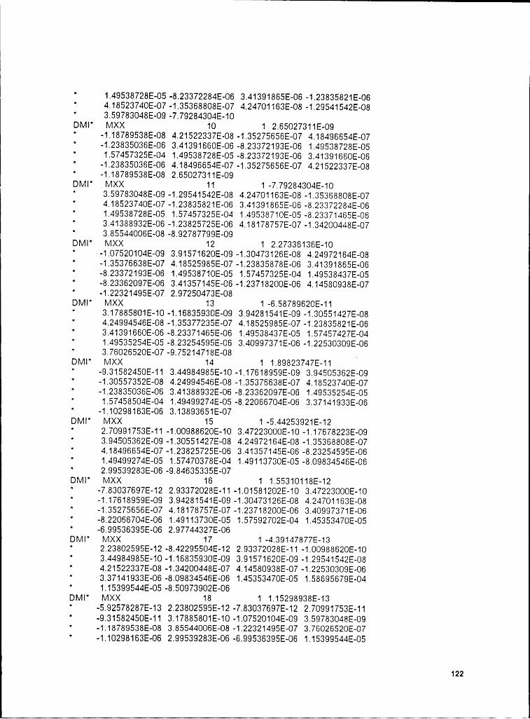
II

" 1.49538728E-05 -8.23372284E-06 3.41391865E-06 -1.23835821E—06" 4.18523740E-07 -1.35368808E-07 4.24701163E-08 -1.29541542E-08* 3.59783048E~09 -7.79284304E-10DM|" MXX 10 1 2.65027311E-09* -1.18789538E·08 4.21522337E—08 —1.35275656E-07 4.18496654E-07* —1.23835036E·06 3.41391660E—06 -8.23372193E-06 1.49538728E—05* 1.57457325E-04 1.49538728E~05 -8.23372193E-06 3.41391660E-06' ·1.23835036E-06 4.18496654E-07 -1.35275656E-07 4.21522337E—08* —1.18789538E-08 2.65027311E-09D|\/II* MXX 11 1 -7.79284304E—10' 3.59783048E—09 -1.29541542E-08 4.24701163E-08 —1.35368808E—07' 4.18523740E—07 -1.23835821E-06 3.41391865E-06 -8.23372284E-06* 1.49538728E-05 1.57457325E-04 1.49538710E-05 —8.23371465E-06' 3.41388932E-06 -1.23825725E-06 4.18178757E~07 -1.34200448E-07* 3.85544006E—08 -8.92787799E-09DMI* MXX 12 1 2.27336136E—10' —1.07520104E-09 3.91571620E—09 -1.30473126E-08 4.24972164E—08" ~1.35376638E·07 4.18525985E-07 -1.23835878E-06 3.41391865E·06* -8.23372193E-06 1.49538710E—05 1.57457325E-04 1.49538437E-05' -8.23362097E-06 3.41357145E-06 -1.23718200E-06 4.14580938E-07* -1.22321495E-07 2.97250473E-08DM|* IVIXX 13 1 -6.58789620E-11" 3.17885801E—10 -1.16835930E-09 3.94281541E-09 -1.30551427E-08* 4.24994546E-08 ·1.35377235E-07 4.18525985E—07 ·1.23835821E-06* 3.41391660E-06 -8.23371465E-06 1.49538437E-05 1.57457427E-04* 1.49535254E·05 -8.23254595E—06 3.40997371E-06 -1.22530309E-06" 3.76026520E·07 —9.75214718E-08 _DI\/1I* MXX 14 1 1.89823747E·11" -9.31582450E-11 3.44984985E-10 -1,17618959E-09 3.94505362E-09* —1.30557352E—08 4.24994546E—08 -1.35376638E-07 4.18523740E-07* ·1.23835036E-06 3.41388932E-06 -8.23362097E-06 1.49535254E—05* 1,57458504E-04 1.49499274E-05 -8.22066704E—06 3.37141933E—06* -1.10298163E-06 3.13893651E-07D|\/||' I\/IXX 15 1 -5.44253921E-12* 2.70991753E-11 -1.00988620E—10 3.47223000E-10 —1.17678223E-09" 3.94505362E-09 -1.30551427E—08 4.24972164E-08 -1.35368808E-07* 4.18496654E-07 -1.23825725E-06 3.41357145E—06 -8.23254595E—06* 1.49499274E·05 1.57470378E·04 1.49113730E·05 -8.09834546E-06* 2.99539283E-06 -9.84635335E-07DM|* I\/IXX 16 1 1.55310118E-12" ·7.83037697E-12 2.93372028E·11 -1.01581202E-10 3.47223000E-10* -1.17618959E—09 3.94281541E-09 ~1.30473126E—08 4.24701163E-08* -1.35275656E-07 4.18178757E—07 -1.23718200E—06 3.40997371E-06* -8.22066704E-06 1.49113730E-05 1.57592702E-04 1.45353470E-05" -6.99536395E·06 2.97744327E-06DI\/II" |\/IXX 17 1 -4.39147877E-13* 2,23802595E-12 -8.42295504E-12 2.93372028E-11 -1.00988620E-10* 3.44984985E—10 -1.16835930E-09 3.91571620E—09 -1.29541542E—08* 4.21522337E-08 -1.34200448E-07 4.14580938E-07 -1.22530309E—06" 3.37141933E—06 -8.09834546E-06 1.45353470E-05 1.58695679E—04" 1.15399544E—05 -8.50973902E-06DM|* MXX 18 1 1.15298938E-13' —5.92578287E-13 2.23802595E-12-7.83037697E-12 2.70991753E—11" -9.31582450E—11 3.17885801E-10 ·1.07520104E-09 3.59783048E-09* -1.18789538E~08 3.85544006E-08 -1.22321495E-07 3.76026520E-07' ·1.10298163E-06 2.99539283E—06 -6.99536395E-06 1.15399544E—05

122

+l+

" 1.65691046E-04 2.30934056E-05DMI* MXX 19 1 ·2.19724700E-14* 1.15298938E-13 -4.39147877E-13 1.55310118E-12 -5.44253921E-12* 1.89823747E-11 -6.58789620E-11 2.27336136E-10 -7.79284304E-10* 2.65027311E-09 -8.92787799E—09 2.97250473E-08 -9.75214718E-08* 3.13893651E-07 -9.84635335E-07 2.97744327E-06 -8.50973902E-06" 2.30934056E-05 4.09468739E-05DMI KXX 0 6 1 0 19 19DMI* KXX 1 1 9.81256714E+02* -2.22544043E +03 1.57756165E +03 —4.22706390E +02 1.13263832E + 02* -3.03489532E +01 8.13197708E +00 —2.17895675E +00 5.83849728E-01' -1.56442061E-01 4.19185236E-02 -1.12320343E-02 3.00961407E-03* —8.06422264E-04 2.16074855E-04 -5.78771942E-05 1.54339195E-05* -3.85847989E-06 6.43079943E-07DM|* KXX 2 1 -2.22544043E +03* 6.02844238E +03 -5.80327002E +03 2.53623828E + 03 -6.79583008E +02" 1.82093719E +02 ·4.87918663E +01 1.30737410E +01 -3.50309825E +00* 9.38652337E-01 -2.51511127E~01 6.73922077E-02 -1.80576853E-02" 4.83853370E-03 -1.29644922E-03 3.47263180E-04 -9.26035136E-05" 2.31508784E-05 -3.85847989E-06DM|* KXX 3 1 1.57756165E+03* -5.80327002E + 03 8.56468066E + 03 -6.48285303E + 03 2.71833203E + 03* -7.28374878E +02 1.95167465E +02 -5.22949638E +01 1.40123930E +01' -3.75460935E +00 1.00604451E +00 -2.69568831E-01 7.22307414E-02* -1.93541348E-02 5.18579688E-03 —1.38905272E-03 3.70414054E-04* -9.26035136E-05 1.54339195E-05DM|* KXX 4 1 -4.2270639OE +02' 2.53623828E + 03 -6.48285303E +03 8.74677441E +03 -6.53164502E +03* 2.73140576E +03 -7.31877991E +02 1.96106110E +02 -5.25464745E +01' 1.40797853E+01 —3.77266717E+00 1.01088309E+00 -2.70865262E-01* 7.25780055E·02 -1.94467381E-02 5.20894770E—03 —1.38905272E-03' 3.47263180E-04 -5.78771942E-05DMI" KXX 5 1 1.13263832E+02' -6.79583008E +02 2.71833203E +03 -6.53164502E + 03 8.75984863E +03* -6.53514795E + 03 2.73234448E + 03 -7.32129456E + 02 1.96173508E + 02* -5.25645332E +01 1.40846233E +01 -3.77396345E + 00 1.01123035E +00* -2.70957887E-01 7.26011544E-02 -1.94467381E-02 5.18579688E-03' -1.29644922E-03 2.16074855E-04DM|* KXX 6 1 -3.03489532E +01* 1.82093719E +02 -7.28374878E +02 2.73140576E + 03 -6.53514795E +03* 8.76078711E +03 -6.53539990E +03 2.73241187E + 03 -7.32147522E +02* 1.96178345E + 02 -5.25658264E +01 1.40849714E +01 -3.77405620E +00* 1.01125348E+00 -2.70957887E-01 7.25780055E·02 -1.93541348E-02* 4.83853370E-03 -8.06422264E-04DM|* KXX 7 1 8.13197708E+00* -487918663E +01 1.95167465E +02 -7.31877991E +02 2.73234448E + 03* -6.53539990E +03 8.76085449E +03 ·6.53541797E +03 2.73241675E +03* -7.32148804E +02 1.96178680E +02 -5.25659218E + 01 1.40849943E +01* -3.77405620E+00 1.01123035E+00 -2.70865262E-01 7.22307414E-02* -1.80576853E-02 3.00961407E-03DM|' KXX 8 1 —2.17895675E +00' 1.30737410E +01 -5.22949638E +01 1.96106110E +02 -7.32129456E + 02' 2.73241187E +03 ·6.53541797E +03 8.76085938E +03 -6.53541895E +03' 2.73241699E +03 -7.32148926E +02 1.96178711E +02 -5.25659218E +01" 1.40849714E +01 -3.77396345E +00 1.01088309E +00 -2.69568831E-01" 6.73922077E—02 -1.12320343E-02

123

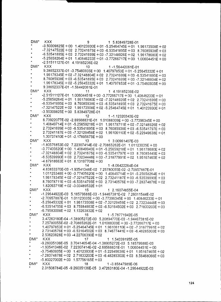
DMI* KXX 9 1 5.83849728E-01* -3.50309825E+00 1.40123930E +01 -5.2546474SE +01 1.96173508E +02" -7.32147522E +02 2.73241675E +03 -6.53541895E +03 8.76085938E +03* -6.53541895E +03 2.73241699E +03 -7.32148926E + 02 1.96178680E +02° -5.25658264E +01 1.40846233E +01 —3.77266717E +00 1.00604451E +00* -2.51511127E-01 4.19185236E-02DM|* KXX 10 1 -1.56442061E—01* 9.38652337E—01 ·3.75460935E +00 1.40797853E +01 -5.25645332E +01* 1.96178345E +02 -7.32148804E +02 2.73241699E +03 -6.53541895E +03* 8.76085938E + 03 -6.53541895E + 03 2.73241699E + 03 -7.32148804E +02' 1.96178345E + 02 -5.25645332E +01 1.40797853E +01 ·3.75460935E + 00* 9.38652337E—01 -1.56442061E—01DMI* KXX 11 1 4.19185236E-02* -2.51511127E-01 1.00604451E +00 —3.77266717E +00 1.40846233E +01" -5.25658264E +01 1.96178680E +02 -7.32148926E + 02 2.73241699E + 03" -6.53541895E +03 8.76085938E +03 -6.53541895E +03 2.73241675E +03* -7.32147522E +02 1.96173508E +02 -5.25464745E +01 1.40123930E +01" -3.50309825E+00 5.83849728E-01DMI* KXX 12 1 -1.12320343E-02* 6.73922077E—02 -2.69568831E-01 1.01088309E +00 -3.77396345E +00* 1.40849714E +01 -5.25659218E +01 1.96178711E +02 -7.32148926E +02* 2.73241699E +03 -6.53541895E +03 8.76085938E + 03 -6.53541797E +03" 2.73241187E +03 -7.32129456E +02 1.96106110E +02 -5.22949638E +01' 1.30737410E+01 -2.17895675E+00DM|" KXX 13 1 3.00961407E-03* -1.80576853E-02 7.22307414E-02 -2.70865262E-01 1.01123035E+00" -3.77405620E +00 1.40849943E +01 -5.25659218E +01 1.96178680E +02" -7.32148804E +02 2.73241675E +03 -6.53541797E + 03 8.76085449E +03" -6.5353999OE +03 2.73234448E + 03 -7.31877991E +02 1.95167465E + 02" -4.87918663E+01 8.13197708E +00DM|" KXX 14 1 -8.06422264E-04* 4.83853370E-03 -1.93541348E-02 7.25780055E-02 -2.70957887E-01' 1.01125348E +00 -3.77405620E + 00 1.40849714E +01 -5.25658264E +01* 1.96178345E + 02 -7.32147522E +02 2.73241187E +03 -6.53539990E +03* 8.76078711E + 03 -6.53514795E +03 2.73140576E + 03 -7.28374878E + 02' 1.82093719E+02 —3.03489532E +01DM|* KXX 15 1 2.16074855E-04* -1.29644922E-03 5.18579688E-03 -1.94467381E-02 7.26011544E—02* -2.70957887E—01 1.01123035E + 00 -3.77396345E +00 1.40846233E + 01" -5.25645332E +01 1.96173508E + 02 -7.32129456E + 02 2.73234448E +03* -6.53514795E +03 8.75984863E +03 -6.53164502E +03 2.71833203E + 03* -6.79583008E+02 1.13263832E +02D|\/1|" KXX 16 1 -5.78771942E-05" 3.47263180E-04 -1.38905272E-03 5.20894770E-03 -1.94467381E-02* 7.25780055E-02 -2.70865262E-01 1.01088309E+00 —3.77266717E +00* 1.40797853E +01 -5.25464745E +01 1.96106110E +02 -731877991E + 02

2.73140576E+03 -6.53164502E +03 8.74677441E+03 -6.48285303E+03* 2.53623828E+03 ·4.22706390E+02DMI" KXX 17 1 1.54339195E·05* ·9.26035136E-05 3.70414054E—04 -1.38905272E-03 5.18579688E-03" -1.93541348E-02 7.22307414E-02 -2.69568831E-01 1.00604451E+00* ·3.75460935E +00 1.40123930E +01 -5.22949638E + 01 1.95167465E +02* -7.28374878E +02 2.71833203E +03 -6.48285303E +03 8.56468066E +03* -5.80327002E+03 1.57756165E+03DM|* KXX 18 1 -3.85847989E-06’ 2.31508784E-05 -9.26035136E-05 3.47263180E-04 -1.29644922E-03

124 ,1

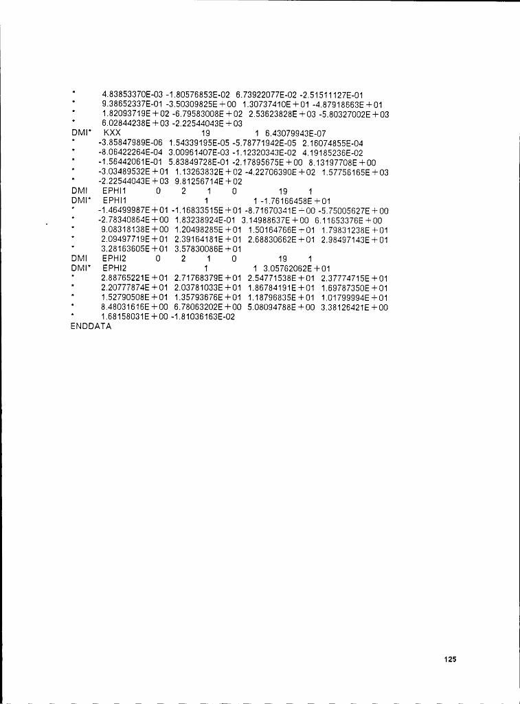
I

I' 4.8385337OE·03 -1.80576853E·02 6.73922077E-02 -2.51511127E—01* 9.38652337E-01 -3.50309825E—I—00 1.3073741OE—I—01 -4.87918663E+01" 1.82093719E+02 -6.79583008E—I-02 2.53623828E+03 -5.80327002E+03* 6.02844238E—!-O3 —2.22544043E+03DM!* KXX 19 1 6.43079943E-07* -3.85847989E—O6 1.54339195E-05 -5.78771942E-05 2.16074855E-04* -8.06422264E-04 3.00961407E-03 -1.12320343E·02 4.19185236E-02* -1.56442061E-O1 5.83849728E-O1-2.17895675E—!—O0 8.13197708E-I-00' -3.03489532E·!—01 1.13263832E+02 -4.2270639OE-I-02 1.57756165E—I—03* —2.22544043E—!—03 9.81256714E—I—02DM! EPHI1 0 2 1 0 19 1DM|* EPH!1 1 1 -1.76166458E +01* -1.46499987E-I-01 ·1.16833515E—+—01 -8.71670341E-!·O0 -5.75005627E-+-00_ * -2.78340864E+00 1.83238924E~01 3.14988637E-I-00 6.11653376E—I—O0* 9.08318138E-I-00 1.20498285E-I-O1 1.50164766E+01 1.79831238E+01* 2.09497719E-+-01 2.39164181E—!—01 2.68830662E+01 2.98497143E-+-01* 3.28163605E+01 3.57830086E+01DM! EPH!2 0 2 1 0 19 1DM|* EPHI2 1 1 3.05762062E+01" 2.88765221E—!—01 2.71768379E+01 2.54771538E-I-01 2.37774715E+01" 2.20777874E+01 2.03781033E—+—01 1.86784191E+01 1.69787350E-I-01" 1.52790508E—+—01 1.35793676E-I-01 1.18796835E-I-01 1.01799994E+01* 8.48031616E+00 6.78063202E—I—00 5.08094788E+00 3.38126421E+O0* 1.68158031E—!—00 -1.81036163E-02ENDDATA

125

A.2 SoIut1on Sequence for Orthogonahty Based MethodID MSC,NASTRAN SPASSOL 63TIME 100SSS 1.)S ALTER 1134 S IBMALTER 1159 S VAXSSS 2.) RENAME MASS AND STIFFNESS MATRICESMATMOD PHIX,,,,,/EPHI1,/1/1MATMOD PHIX,,,,,/EPHI2,/1/2MATPCH EPHI1,EPHI2// SADD MXX,/MAADD KXX./KATRNSP EPHI/EPHITADD EPHI,/NPHISS 3.) EXTRACT ORIGINAL FREOUENCY VALUESLAMX ,,LAMA/LAMM/-1MATMOD LAMM,,,,,/OF,/1/3SS 4.) GENERATE LMATRNSP NPHI/NPHIT SSMPYAD NPHIT,MA,NPHI,,,/LMA/3 SSS 5.) GENERATE UPDATED MASS MATRIXMATMOD NPI-IIT,,,,,/IT,/28DIAGONAL IT/I/SOUARE/0.ADD I,LMA/IMLMA//(-1.0,0.0) SSOLVE LMA,/LMAI SSMPYAD NPHI,LMAI,IMLMA,LMAI,NPHIT,/MTEMP/5 SSMPYAD MA,MTEMP,MA,,,MA/MNEW/3 SSS 6.) GENERATE UPDATED STIFFNESS MATRIXMATMOD EF,,,,,/EFT,/28ADD EFT,/EFM/(6.28318500) SDIAGONAL EFM/EOME2/SOUARE/2.SMPYAD KA,NPHI,NPH|T,MNEW,,/KT1/4 SSMPYAD NPHIT,KA,NPHI,,,EOME2/KT2/3 SSMPYAD MNEVV,NPHI,KT2,NPHIT,MNEVV,/KT3/5 SADD KT3,KT1/DEL/(.5,0.0)/(-1.0,0.0) STRNSP DEL/DELT SADD5 DEL,DELT,KA,,/KNEWSSS 7.) EXTRACT NEWLY CALCULATED EIGENVALUES AND EIGENVECTORSSETVAL //V,N,NEIGVS/-1 SREAD KNEW,MNEW,MR,DMX,EED,VXCOMPR,CASES/LAMA,NPH|X,MI,OEIGS/ V,N,

READAPP= MODES/S,N,NEIGVS SOFP LAMA,OEIGS// SLAMX ,,LAMA/LAMM/-1

126

I

I

MATMOD LAMM,,,,,/NEWF,/1/3$$ 8.) PRINT ORIGINAL FE DATA, EXPERIMENTAL DATA, UPDATED DATAADD MXX,MNEW/DELM/-1.ADD KXX,KNEW/DELK/-1.MATPRN MA,MNEVV,KA,KNEW//$$ MATPRN PHIX,NPHI,NPHIX// $MATPRN OF,EF,NEWF// $$$DIAGONAL MXX/ALLONE/WHOLE/0.ADD MXX.MNEW/MDIF//-1.ADD MXX,MDIF/MPERC///2ADD KXX,KNEVI//KDIF//-1.ADD KDIF,KXX/KPERC///2MATPRN MDIF,KDIF// $MATPRN MPERC,KPERC// $MATPCH NPHIX// $$CEND$TITLE = IMPROVEMENT OF A LARGE ANALYTICAL MODEL USING TEST DATASUBTITLE = UTILIZING BERMAN AND NAGY’S METHODLABEL = CANTILEVER BEAM 10 x 1 x .1$$METHOD = 10SEALL = ALLDISPLACEMENT = ALL$SPC = 1$BEGIN BULK$$$PARAM , COUPMASS , 1

$EIGR ,10 , MGIV,,,,10ASET1 , 2 , 1 ,THRU , 19GRDSET,,,,,, , 1345GRID ,1, ,0. ,0.,0.= I’<1>I = I ’<2I> I = I ==<17)CBAR, 1,1,1, 2,0.0,1.0= I’<1)I= I’<1>I‘(1>I = I==<16)CONM2 , 101 , 1 , , 0.0000294= I'<1> I '<1>I = I ==<16>PBAR , 1 ,1 ,.1 , 1.6276-4, .01MAT1 1 30.0+6 0.33 7.324-4$DMI,EF,0,2,1,0,,8,1DMI , EF , 1 , 1 ,0.00001 ,0.00001 ,20.07, 55.31 , 108.4,

127

1

é 179.2 , 267.7, 374.0DMI EPHI 0 2 1 0 19 8$$$ NORMAILIZED TEPHINBULK TO NEW MASS MATRIXDM|" EPHI 1 1 1.00000000E+01' 0.00000000E+01 1.00000000E+01 0.00000000E+01 1.00000000E+01* 0.00000000E+01 1.00000000E +01 0.00000000E +01 1.00000000E+01* 0.00000000E+01 1.00000000E+01 0.00000000E +01 1.00000000E+01" 0.00000000E+01 1.00000000E+01 0.00000000E+01 1.00000000E+01" 0.00000000E+01 1.00000000E+01DMI* EPHI 2 1 0.00000000E+01' 1.00000000E +01 0.00000000E+01 1.00000000E+01 0„00000000E+01* 1.00000000E+01 0.00000000E +01 1.00000000E+01 0.00000000E+01* 1.00000000E+01 0.00000000E+01 1.00000000E+01 0.00000000E +01* 1.00000000E+01 0.00000000E+01 1.00000000E +01 0.00000000E +01' 1.00000000E+01 0.00000000E +01DMI' EPHI 3 1 -3.18472538E +01 ”* -2.65386353E+01 -1.74418297E+01 ·7.80900669E +00 7.23694801E-01* 8.34104633E+00 1.47938519E+01 1.92597923E+01 2.05792141E+01* 2.00870094E+01 1.93061790E+01 1.71260357E-I-01 1.27322531E +01* 6.72526789E+00 4.22959059E·01 -9.35005283E+00 —1.91838799E+01" -2.93217945E+01 -3.55065918E+01DMI" EPHI 4 1 -3.10419502E+01’ -1.97756252E +01 -3.90104151E+00 1.16861610E+01 1.99744129E+01" 2.36747532E+01 2.47047443E+01 2.03940392E+01 1.18374815E+01* 3.20117235E-01 -1.13767452E+01 —1.96993294E+01 -2.32089310E+01" —2.31072025E+01 -1.89236565E+01 -9.69569778E+00 4.95942736E+00" 2.15766220E +01 2.88247108E+01DMI' EPHI 5 1 3.03047791E+01* 1.48218765E+01 -8.48413849E +00 -2.02269726E+01 -1.97451744E+01* -1.71320267E +01 -6.27276182E +00 9.76706886E+00 1.84639530E+01* 2.31594524E+01 1.80964794E +01 9.93039036E+00 -6.31930876E+00* -1.79159698E+01 -2.01534786E +01 -1.90510578E+01 -7.85290003E+00* 1.33846464E+01 4.39258118E+01DMI" EPHI 6 1 -1.82504902E+01* -4.54117727E+00 2.10175896E +01 2.59855595E+01 1.73300571E+01* -2.73532486E+00 -2.14730549E +01 -2.72171612E-I-01 -1.73849392E +01* -1.74101532E+00 1.88608665E+01 2.18974438E +01 2.31886177E+01* 1.21079671E+00 -1.75494652E+01 -2.43987560E +01 -1.96883049E+01* 6.26746941E+00 2.74698696E+01DMI* EPHI 7 1 ·2.27725697E+01' 9.27494705E—01 2.12805443E+01 1.83374405E+01 -7.78031707E—01" -2.46232395E+01 —2.74261951E+01 —9.07402515E+00 1.25015440E+01* 2.883-41484E+01 1.09958544E+01 -8.53858852E +00 -3.09406681E+01* -2.30169296E+01 -5.80351472E-01 1.92681656E+01 2.15572453E+01" —1.20835721E+00 -2.52521076E+01DMI* EPHI 8 1 2.42963963E+01* -9.11770344E+00 —2.06297493E+01 -9.88259411E+00 1.85433483E+01* 2.50731907E +01 6.63844204E+00 -2.25553684E+01 —2.55435009E+01* -2.15928182E-01 1.97695541E+01 2.15910053E +01 —5.65337563E+00' -2.59304104E +01 -1.84511528E +01 1.51534271E+01 2.32457867E+01* 6.85273027E +00 -3.25167999E +01ENDDATA

128

1I

A.3 Solutmn Sequence for Connectmty Constramt BasedMethodID MSC,NASTRAN $PASSOL 63TIME 100$$ 1)$ ALTER 509 $ SOL 3ALTER 1159 $ SOL 63$PARAM //NOP/V,Y,KLOOP=1$PARAM //ADD/\/,Y,KLOOP1/V,Y,NN=0/1PARAM //ADD/V,Y,NNM1/V,Y,NN=0/-1PARAM //ADD/V,Y,NNM2/V,Y,NN=0/-2PARAM //ADD/V,Y,NNP1/V,Y,NN=0/1PARAM //SUB/V,Y,NNN/0/V,Y,NN=0PARAM //SUB/V,Y,NNNP1/0/V,Y,NNP1PARAM //NOP/V,Y,KLOOP6=1PARAM //ADD/V,Y,KLOOP7/V,Y,NNP1/0$PARAM //NOP/V,Y,KLOOP2=2PARAM //NOP/V,Y,NEGONE=—1PARAM //NOP/\/,Y,KLOOP3=1PRTPARM //0/C,N,NNI PRTPARM //0/C,N.NNM1PRTPARM //0/C,N,NNM2PRTPARM //0/C,N,NNP1PRTPARM //0/C,N,NNNPRTPARM //0/C,N,NNNP1$$ 2.) STORE MATRICES FROM DMIADD KXX,/KAADD MXX,/MAADD EPHI,/EPHIN$$ 3.) GENERATE EXPERIMENTAL EIGENVLAUESPRTPARM //0/C,N,LAMMEXEMATMOD EF,,,,,/EF1,/28ADD EF1,/EF2/(6.283185,0.0) $DIAGONAL EF2/OMEGANE/SOUARE/2.$$ 4.) GENERATE A FROM SYSTEM DATAPRTPARM //0/C,N,AGENMPYAD I<XX,EPHI,/TEMPSMPYAD MXX,EPHI,OMEGANE,,,TEMP/ATEMP/3//-1ADD ATEMP,/A/4.$ .$ 5.) GENERATE CAP PHI FROM ORIGINAL K MATRIXPRTPARM //0/C,N,CPHGENADD KXX,/KXX2ADD KXX,KXX2/CAPPH|///C,Y,IOPT=1$$ 6.) GENERATE PARTITIONING VECTORS

129

PRTPARM //0/C,N,CPHPARTTRNSP CAPPHI/CAPPHITTRNSP A/ATTRNSP EPHI/EPHITDIAGONAL KXX/NZTEMP/C,Y,COLUMN/V,Y,POV\/ER=0.$ADD NZTEMP,/NZ/(0.0,0.0)TRNSP NZTEMP/NZTEMPTTRNSP NZ/NZTMATMOD NZTEMPT,,,,/ONEONES,/1/1ADD ONEONES,/ONEONEMATMOD NZT,,,,/ONEZERO,/1/1DIAGONAL KXX/NONES/C,Y,COLUMN/V,Y,POWER=0.$MPYAD EPI—IIT,EPHl/MBYMDIAGONAL MBYM/MONES/C,Y,COLUMN/V,Y,POWER=0.$ADD MONES,/MZEROS/(0.0,0.0)TRNSP MONES/MONESTTRNSP MZEROS/MZEROSTDBSTORE CAPPHI,EPHI,EPHIT,KXX,MXX//1/1$DBSTORE MONES,MZEROS,A,OMEGANE//1/1$DBSTORE KA,MA//1/1$FILE ONEZEROS=APPENDFILE MZEROST=APPENDFILE ABART=APPENDFILE GPVTEMP=APPENDFILE VPGTEMP=APPENDFILE MMMTEMP=APPEND$$ 7.) SET UP LOOP TO GENERATE MATRICESLABEL KTOP1

PRTPARM //0/C,N,KLOOPPARAM //ADD/V,Y,KLOOPP1/V,Y,KLOOP/1

$$ 8.) EXTRACT ROWS FROM CAPPHI

PRTPARM //0/C,N,Z1MATMOD CAPPHIT,,,,,/T1,/1/KLOOPMATMOD T1,,,,,/CPHI,/28

8$ 9.) GENERATE ABAR FROM A

PRTPARM //0/C,N,Z2MATMOD AT,,,,,/ACOL,/1/KLOOPTRNSP ACOL/ACOLTAPPEND ACOLT,/ABART/2

$$ 10.) GENERATE G SUP I

PRTPARM //0/C,N,Z3SMPYAD EPHIT,CPI—II,EPHI,,,/NGG/3

$$ 11.) GENERATE EPHR#

PRTPARM //0/C,N,Z4MATMOD EPHIT,,,,,/EPHR,/1/KLOOP

$$ 12.) GENERATE M##

PRTPARM //0/C,N,Z5APPEND ONEONES,/MMMTEMP/2

130

I

I

ADD MMMTEMP,/MMM$$ 13.) GENERATE G PARTITIONING VECTOR

PRTPARM //0/C,N,GGGAPPEND MZEROST,/GPVTEMP/2ADD GPVTEMP,/GPVAPPEND MONEST,/VPGTEMP/2ADD VPGTEMP,/VPGPRTPARM //O/C,N,BCDDBSTORE GPV.MMM//KLOOPP1/1DBSTORE VPG,CPH|,NGG,EPHR//KLOOP/1PARAM //ADD/V,Y,KLOOP/V,Y,KLOOP/1PARAM //SUB/V,N,FLAG/V,Y,NN/V,Y,KLOOPCOND DUT,FLAG

REPT KTOP1,1000 $ # CORRESPDNDS TO(N-1). CHANGELABEL OUTTRNSP ABART/ABARDBSTORE ABAR//1/1$$$ 14.) ASSEMBLE ALPHA MATRIXADD NZ,ONEONE/MNUMDBSTORE MNUM,,,,//1/1DBFETCH /NGG,,,,/1/1ADD NGG,/NALPHT1LABEL KTOP2

PRTPARM //0/C,N,KLODP2DBFETCH /NGG,GP\/,GPVTEMP,MMM,MMMTEMP/KLOOP2/1APPEND GPV,MONEST/GPV1T/0TRNSP GPV1T/GPV1MERGE NALPHT1,,,NGG,GPV1/NALPHT2/-1/0/V,Y,FORMPURGE NALPHT1/ALWAYSPURGE NALPHT1/NE\/ERADD NALPHT2,/NALPHT1PURGE NALPHT2/ALVVAYSPURGE NALPHT2/NEVERADD MMM,/MMM1/(0.0,0.0)APPEND MMM1,0NEONES/MNUM1/0TRNSP MNUM1/MNUM1TADD NZ,MNUM1T/MNUMDBSTORE MNUM//KLOOP2/1PARAM //ADD/V,Y,KLOOP2/V.Y,KLOOP2/1PARAM //SUB/V,N,FLAG/V,Y,NN/V,Y,KLOOP2COND OUT2,FLAG

REPT KTOP2,1000 $ CORRESPONDS TO (N-2) CHANGELABEL OUT2ADD NALPHT1,/ALPHA/(-1.0,0.0)MATPRN ALPHA//$$$ 15.) GENERATE BETA MATRIXPRTPARM //0/C,N,BGEN

· FILE HROW=APPENDFILE BETA=APPENDLABEL KTOP6

PRTPARM //0/C,N,KLOOP6DBFETCH /MNUM,,,,/KLOOP6/1MATMOD MNUM,,,,,/MNUMM,/28

131

1I,

PARAM //ADD/V,Y,KLOOP7/V,Y,KLOOP7/V,Y,NNN $ CORRESPONDS TO (-N).LABEL KTOP7

PRTPARM //O/C,N,KLOOP7DBFETCH /EPHR,CPHI,,,/KLOOP7/1TRNSP NONES/NONESTSMPYAD EPHR,NONEST,MNUMM,CPHI,EPH|N,/HCN/5/-1APPEND HCN,/HROVV/2PURGE HCN/ALVVAYSPURGE HCN/NEVERPARAM //ADD/V,Y,KLOOP7/V,Y,KLOOP7/1PARAM //SUB/V,N,FLAG/V,Y,NN/V,Y,KLOOP7COND OUT7,FLAG

REPT KTOP7.100 $ # CORRESPONDS TO (N-1). CHANGELABEL OUT7TRNSP HROVV/HROWTAPPEND HROVVT,/BETA/2PURGE HROVV/ALVVAYSPURGE HROW/NEVERPARAM //ADD/V,Y,KLOOP6/V,Y,KLOOP6/1PARAM //SUB/V,N,FLAG/V,Y,NN/V,Y,KLOOP6$COND OUT6,FLAG

REPT KTOP6,1000 $ CORRESPONDS TO (N-1). CHANGELABEL OUT6DBSTORE BETA//1/1$MATPRN BETA// $$$ 16.) FIND EIGENDATA OF ALPHA -I— BETAADD ALPHA,BETA/AB $SETVAL //V,N,NElGV/·1 $DIAGONAL ALPHA/IA/SOUARE/O.DBSTORE AB,IA//1/1$ADD IA,/NIA/-1.READ AB,IA,,,DYNAMICS,,CASECC/ABLA,ABPH,ABM|,ABOE/MODES/S,N,NEIGV $OFP ABLA,ABOE// $LAMX ,,ABLA/ABLAMM/-1MATMOD ABLAMM,,,,,/OMEGAV,/1/1MATMOD OMEGAV,,,,,/OMEGAB,/28ADD ABLAMM,/NABLAMM/-1.$$ 17.) PURGE MODAL MATRICES OF ZERO EIGENVALUES AND CORRESPONDING E. VEC.PRTPARM //O/C,N,MODMODALPARTN ABPH,ABP\//,,ABPHN,/0PARTN OMEGAB,ABPV,/,,,OMEGABN/-1$$18.) GENERATE LAMBDA BPRTPARM //O/C,N,LAMBGENSOLVE OMEGABN,/OMEGAINVTRNSP ABPHN/ABPHNTSMPYAD ABPHN,OMEGAINV,ABPHNT,ABAR,,/LAMBDAB/4MATPRN LAMBDAB// $S$19.) GENERATE LAMBDA FROM LAMBDA BPRTPARM //0/C,N,LAMKGENFILE LAMBDAT=APPENDADD LAMBDAB,/LTEMP2

132

DBSTORE LTEMP2//1/1LABEL KTOP3

PRTPARM //0/C,N,KLOOP3PARAM //ADD/V,Y,KLOOP3NT/V,Y,NNNP1/V,Y,KLOOP3 $ TO -(N -+-1). CHANGEPARAM //ADD/V,Y,KLOOP3P1/V,Y,KLOOP3/1PRTPARM //0/C,N,HEREPARAM //MPY/V,Y,KLOOP3N/V,Y,KLOOP3NT/V,Y,NEGONEPRTPARM //0/C,N,KLOOP3NTPRTPARM //0/C,N,KLOOP3NDBFETCH /VPG,VPGTEMP,,,/KLOOPBN/1TRNSP VPG/\/PGTADD \/PGT,MONES/GPV2//(-1.0,0.0)DBFETCH /LTEMP2,,,,/KLOOP3/1ADD LTEMP2,/LTEMPPARTN LTEMP,,GPV2/LLL.LTEMP2,,/0DBSTORE LTEMP2//KLOOP3P1/1APPEND LLL,/LAMBDAT/2PRTPARM //0/C,N,HEREPARAM //ADD/\/,Y,KLOOP3/V,Y,KLOOP3/1PARAM //SUB/V,N,FLAG/V,Y,NN/V,Y,KLOOP3COND OUT3,FLAG

REPT KTOP3,1000 $ # CORRESPONDS TO (N—1) CHANGELABEL OUT3$TRNSP LAMBDAT/LAMBDAMATPRN LAMBDA// $DBSTORE LAMBDA// $$$ 20.) GENERATE NEW K MATRIXPRTPARM //0/C,N,NEWKGENTRNSP LAMBDA/LAMBDATMPYAD EPI-II,LAMBDAT,/KT1AMPYAD LAMBDA,EPHIT,/KT1BADD KT1A,KT1B/KT2ADD CAPPHI,KT2/KT3///C,Y,IOPT=1ADD KA,KT3/KNEW//(-.25,0.0)$$ 21.) PERFORM FINAL EIGENVALUES ANALYSISPRTPARM //0/C,N.FINALEIGENSETVAL //V,N,NEIGV/-1$READ KNEW,MXX,,,DYNAMICS,,CASECC/ABL,ABPH,ABMI,ABOE/MODES/S,N,NEIGV $OFP ABL,ABOE// $MATPRN EF,EPHI//$MATPRN ABPI-I//$MATPRN KNEW,MXX//$$$ END OF ALTERATIONSCEND$$ ANALYSIS OPTIONSTITLE = STIFFNESS MATRIX ADJUSTMEN USING MODE DATA (CONNECTIVITY)SUBTITLE = UTILIZING A. M. KABE’S METHODMETHOD = 10SEALL = ALLDISPLACEMENT = ALLSPC = 1

133

I

$$ ENTER PHYSICAL DATABEGIN BULK$ä# CHANGE ABOVE ENTRIES TO SUIT # OF NON-ZERO EIGENVALUES$ EXPERIMENTAL DATA OBTAINED FROM UNPERTURBED DATA$ FOR FREE FREE BOUNDARY CONDITIONS$$$EIGR ,10 , MGIV, , ,, 888$$$PARAM , COUPMASS , 1$ASET1 , 2 , 1 , THRU , 19GRDSET,,,,,,, 1345GRID ,1, ,0. ,0.,0.= .‘I1). = (I2-) „ = . ==I17)CBAR, 1,1,1, 2,0.0,1.0= .‘I1),= .’I1)(I1). = .==I16)CONM2 , 101 , 1 , ,0.00002= (I1) „ '<1)„ = .==I16)PBAR , 1 , 1 , .1 , 1.6276—4, .01MAT1 1 30.0+6 0.33 7.324-4$DMI,ABP\/,0,2,1,0,,152,1DMI , ABPV , 1, 98 , 1. , THRU , 152$PARAM , NN , 19$$ CHANGEDMI,EF,0,2,1,0,,8,1DMI , EF, 1 , 1 ,0.00001 ,0.00001 ,20.07 ,55.31 , 108.4 ,

. 179.2 , 267.7 , 374.0$DMI EPHI 0 2 1 0 19 8$ CHANGEDMI* EPHI 1 1-1.72176323E+01* -1.41148415E+01 -1.10120497E +01 -7.90925884E+00 -4.80646753E+00' -1.70367646E+00 1.39911485E+00 4.50190592E+00 7.60469723E+00' 1.07074881E+01 1.38102798E+01 1.69130707E+01 2.00158615E+01* 2.31186543E+01 2.62214451E+01 2.93242359E+01 3.24270287E+01' 3.55298195E+01 3.86326103E+01DMI* EPHI 2 1 —3.46183472E—+01* —3.25617943E+01 -3.05052452E +01 -2.84486923E+01 —2.63921413E+01* -2.43355885E +01 -2.22790375E+01 —2.02224865E+01 —1.81659336E+01* —1.61093826E +01 ·1.40528307E +01 -1.19962788E+01 -9.93972683E+00" -7.88317537E +00 -5.82662344E +00 -3.77007198E +00 -1.71352017E+00* 3.43031585E—01 2.39958334E+00DMl" EPHI 3 1 3.86144180E+01

134

„.,„i..........._ _ - _ LI

I

i " 2.86342773E +01 1.87511196E +01 9.18296051E +00 2.37452328E-01* -7.73347664E+00 -1.43759937E+01 -1.93720779E+01 -2.24709320E+01* -2.35125999E+01 -2.24426174E+01 -1.93169231E+01 -1.42968159E-I-01* -7.63417530E+00 3.52272034E-01 9.30845547E+00 1.88827553E+01* 2.87684174E+01 3.87489510E +01DI\/Il" EPHI 4 1 —3.85642090E+01* -2.17269306E+01-5.56334639E+00 8.57991505E+00 1.91425362E+01’ 2.48533192E+01 2.51050472E+01 2.01576328E+01 1.11488228E+01* ·7.81321302E~02 -1.12895975E+01 -2.02546787E+01 -2.51377831E +01* -2.48122253E +01 -1.90302696E+01 -8.40984535E +00 5.77112436E+00" 2.19516354E+01 3.87917709E+01DI\/Il" EPHI 5 1 3.85213585E+01* 1.50855913E+01 ·5.99615622E+00 —2.06693840E+01 ·2.55651627E+01* -1.99639053E+01-6.45989990E+00 9.75792027E+00 2.26646786E+01* 2.75165100E+01 2.25364819E +01 9.54851818E +00 —6.67327547E+00" -2.01011295E+01 -2.55710430E+01 -2.05314846E +01 -5.74531984E+00" 1.53937120E +01 3.88399200E+01DMI" EPHI 6 1 -3.84950523E+01' -8.61501789E+00 1.54652910E +01 2.55439034E+01 1.84084969E+01 ”" -5.35287321E·01 —1.96334839E +01 -2.74453926E+01 -1.92774658E +01* 1.44958913E-01 1.94827061E+01 2.74463310E+01 1.94306545E +01* 2.49772698E-01 -1.86044827E+01 —2.55246258E+01 -1.52180090E+01" 8.99818039E+00 3.89052696E+01D|\/II' EPHI 7 1 -3.85018806E +01" -2.42385864E+00 2.20858669E +01 2.25441017E +01 1.78078961E+00* -2.12663708E+01 -2.64738045E+01 -9.22068691E +00 1.58506241E+01* 2.73878517E +01 1.55598850E+01 -9.55444622E+00 -2.65665512E-I-01' -2.10404854E +01 2.12887764E +00 2.27075920E +01 2.18992424E+01* -2.86966300E +00 —3.90048752E +01DMP EPHI 8 1 3.85655937E+01" ·3.39209175E+00 -2.53591595E+01 -1.28830242E+01 1.61290245E+01" 2.70523090E+01 6.91272497E-I-00 -2.11531601E +01 -2.47781010E+01* 2.10803017E—01 2.49562874E+01 2.08820953E+01 -7.32034779E+00* —2.71267033E+01 -1.57869587E +01 1.32383242E+01 2.52917023E+01* 2.89967895E+00 —3.91637192E+01ENDDATA

135

I

I I

A.4 SoIut1on Sequence for Res1duaI Force Based MethodID MSC,NASTRAN $PASSOL 63TIME 100$$$ THIS SYSTEM IDENTIFICATION METHOD UTILIZES A RESIDUAL FORCE MATRIX$ TO LOCATE MODELLING ERRORS IN THE FINITE ELEMENT MODEL$ THE METHOD THEN CORRECTS DEFICIENT ELEMENTS ONLY TO UPDATE THE$ SYSTEM MATRICES TO MATCH THE EXPERIMENTAL DATA$$ L IS THE NUMBER OF DEFICIENT ELEMENTS DETERMINED ‘$ M IS THE NUMBER OF EXPERIMENTAL FREOUENCIES$ N IS THE NUMBER OF DOF’S MEASURED$$$ 1.)$ALTER 1159$$ 2.) REARRANGE MATRICESPRTPARM //0/C,N,BEGMODPARAM //ADD/V,Y,MMM1/V,Y,MM=0/-1PARAM //ADD/\/,Y,MMP1/V,Y,MM=0/1PARAM //ADD/V,Y,NNP1/V,Y,NN=0/1PARAM //ADD/V,Y,NNM1/V,Y,NN=0/-1PARAM //NOP/V,Y,I<LOOP=1PARAM //NOP/V,Y,KLOOP4=1PARAM //NOP/V,Y,KLOOP2=1PARAM //NOP/V,Y,KLOOP3=1PARAM //NOP/V,Y,KLOOP5=1PARAM //ADD/V,Y,KNTR/V,Y,NN=0/1MATMOD COM,,,,,/CNM,/28ADD KXX,/KAADD MXX,/MAADD KXX,/OKXXADD MXX,/OMXXDBSTORE OKXX,OMXX//1/1$$$ 3.) THE FOLLOWING MMAT AND KMAT MATRICES NEED TO BE CHANGED FOR THE$ ANALYSIS OF DIFFERENT ENTITIESADD KXX01,/KMATADD MXX01,/MMATDBSTORE KMAT,MMAT//1/1ADD KXX02,/KMATADD MXX02,/MMATDBSTORE KMAT,MMAT//2/1ADD KXX03,/KMATADD MXX03,/MMATDBSTORE KMAT,MMAT//3/1ADD KXX04,/KMATADD MXX04,/MMATDBSTORE KMAT,MMAT//4/1

136

nl

ADD KXX05,/KMATADD MXX05,/MMATDBSTORE KMAT,f\/IMAT//5/1ADD KXX06,/KMATADD MXX06,/MMAT ’DBSTORE KMAT,M|\/IAT//6/1ADD KXX07,/KMATADD MXX07,/NIMATDBSTORE KMAT,|\/1MAT//7/1ADD KXX08,/KMATADD |\/IXXO8,/F\/I|\/1ATDBSTORE KMATMMAT//8/1ADD KXX09,/KMATADD MXX09,/MMATDBSTORE KMAT,I\/1MAT//9/1ADD KXX10,/KMATADD MXX10,/MMATDBSTORE K|\/lAT,|\/H\/IAT//10/1ADD KXX11,/KMATADD I\/IXX11,/|\/I|\/IATDBSTORE KMATMMAT//11/1ADD KXX12,/K|\/IATADD MXX12,/M|\/IATDBSTORE KMATMMAT//12/1ADD KXX13,/KMATADD MXX13,/MMATDBSTORE KMAT,M|\/IAT//13/1ADD KXX14,/KMATADD MXX14,/MMATDBSTORE KMATMMAT//14/1ADD KXX15,/KMATADD MXX15,/MMATDBSTORE KIVIATMMAT//15/1ADD KXX16,/K|\/IATADD MXX16,/MMATDBSTORE K!\/1AT,|\/IMAT//16/1ADD KXX17,/KMATADD MXX17,/|\/IMATDBSTORE KMAT,|\/IMAT//17/1ADD KXX18./KMATADD MXX18,/MMATDBSTORE KI\/|AT,M|\/IAT//18/1$$ 4.) GENERATE OR RENAME ANALYTICAL AND EXPERIMENTAL DATAADD PHIX,/APHINADD EPHI,/EPHINLAMX ,,LAMA/LA|\/1|\/I/-1MATMOD LAMM,,,,,/ALAMV,/1/1MATMOD ALAMV,,,,,/ALAM,/28|\/|AT|\/IOD EF,,,,,/EFT,/28ADD EFT,/EFM/(6.283185,0.0) $DIAGONAL EFM/ELAM/SQUARE/2.ADD APHIN,EF’HIN/DELPHI/-1.ADD ALAM,ELAf\/I/DELLAM/-1.|\/IATPRN DELF°HI,EPH|N,APHIN// $DBSTORE KA,MA,APH|N,EPHIN// $

137

»I

DBSTORE ALAM,ELAM,DELPHI,DELLAM// $MATMOD LAMM,,,,,/AF,/1/3DBSTORE AF,EF// $$$ 5.) MULTIPLY EACH EIGENVECTOR TO ITS CORRESPONDING EIGENVALUELAMX ,,LAMA/LAMM/-1PRTPARM //0/C,N,DEVDBFETCH /EPHIN,,,,/$FILE LPH|=APPENDLABEL KTOP4

MATMOD EPHIN,,,,„/U,/1/KLOOP4SCALAR ELAM//KLOOP4/KLOOP4/S,Y,LADD U,/LU/LAPPEND LU,/LPHI/2PARAM //ADD/V,Y,KLOOP4/V,Y,KLOOP4/1PARAM //SUB/V,N,FLAG/V,Y,MMM1/V,Y,KLOOP4COND OUT4,FLAG

REPT KTOP4,1000 $ # CORRESPONDS TO (M-1). CHANGELABEL OUT4DBSTORE LPHI// $$$ 6.) CALCULATE RESIDUAL FORCE MATRIXPRTPARM //0/C,N,RFMDBFETCH /EPHIN,KA,MA,,/ $MPYAD KA,EF’HIN,/RMT1MPYAD MA,LPHI,/RMT2ADD RMT1,RMT2/RM/-1.MATPRN RM//$DBSTORE RM// $$$ 7.) CALCULATE MATRIX FOR UNKNOVVNSPRTPARM //0/C,N,MUNKGENDBFETCH /APHIN,KA,MA,ALAM,/ $DBFETCH /DELLAM,DELPH|,,,/ $MPYAD KA,DELPHI,/MT1SMPYAD MA,DELPHLELAM,,,MT1/MT2/3//-1SMPYAD MA,APHIN,DELLAM,,,MT2/MUNK/3DBSTORE MUNK// $$$ 8.) GENERATE A MATRIXPRTPARM //0/C,N,AGEN LFILE AKXX=APPENDFILE AMXX=APF’ENDLABEL KTOP1

PRTPARM //0/C,N,KLOOPDBFETCH /KMAT,MMAT,,,/KLOOP/1MPYAD KMAT,EPHIN,/AL1TRNSP AL1/AL1TSMPYAD MMAT,EPHIN,ELAM,,,/AL2/3/-1TRNSP AL2/AL2TPURGE AKXX/NE\/ERPURGE AMXX/NEVERPARAM CORRESPONDS TO (N). CHANGELABEL KTOP2

PRTPARM //O/C,N,KNTRMATMOD AL1T,,,,,/T1,/1/KNTR

138

I

TRNSP T1/T01TAPPEND T01T,/AKXX/2MATMOD AL2T,,,,,/T2,/1/KNTRTRNSP T2/T02TAPPEND T02T,/AMXX/2PARAM //ADD/V,Y,KNTR/V,Y,KNTR/1

PARAM //SUB/V,N,FLAG/V,Y,NN/V,Y,KNTRCOND KNTR1,FLAGREPT KTOP2,1000 S # CORRESPONDS TO (N-1). CHANGELABEL KNTR1DBSTORE AKXX,AMXX//KLOOP/1DBSTORE AKXX//KLOOP/1PURGE AKXX/ALVVAYSPURGE AMXX/ALWAYSPARAM //ADD/V,Y,KLOOF‘/V,Y,KLOOP/1

REPT KTOP1,17 S # CORRESPONDS TO (L—1). CHANGEE LABEL TOHERESMPYAD CNM,EPI·IIN,ELAM,,,/AL2/3/—1TRNSP AL2/AL2TFILE CONMXXT=APPENDLABEL KTOP5

MATMOD AL2T,,,,,/T2,/1/KLOOP5TRNSP T2/T02TAPPEND T02T,/CONMXXT/2PARAM //ADD/V,Y,KLOOP5/V,Y,KLOOP5/1PARAM //SUB/\/,N,FLAG/V,Y,NNM1/\/,Y,KLOOP5COND OUT5,FLAG

REPT KTOP5,1000 S # CORRESPONDS TO (N-1). CHANGELABEL OUT5TRNSP CONMXXT/CONMXX$S 9.) GENERATE B MATRIXPRTPARM //0/C,N,BGENTRNSP MUNK/MUNKTPRTPARM //0/C,N,BGENFILE B1T=AF’PENDLABEL KTOP3

PRTPARM //0/C,N,KLOOP3MATMOD MUNKT,,,,,/T1,/1/KLOOP3TRNSP T1/T01TAPPEND T01T,/B1T/2PARAM //ADD/V,Y,KLOOP3/V,Y,KLOOP3/1PARAM //SUB/V,N,FLAG/V,Y,NN/V,Y,KLOOP3COND OUT3,FLAG

REF’T KTOP3,1000 S # CORRESPONDS TO (N—1). CHANGELABEL OUT3TRNSP B1T/B1DBSTORE B1//1/1 SSS 10.) EXTRACT COLUMNS CORRESPONDING TO DEFICIENT ELEMENTSPURGE AKXX/NEVERPURGE AMXX/NEVERFILE A=AF’PENDDBFETCH /AKXX,,,,/1/1TRNSP AKXX/AC01DBFETCH /AKXX,,,,/2/1

139

TRNSP AKXX/AC02DBFETCH /AKXX,,,,/3/1TRNSP AKXX/AC03DBFETCH /AKXX,,,,/4/1TRNSP AKXX/ACO4DBFETCH /AKXX,,,,/14/1TRNSP AKXX/AC14DBFETCH /AKXX,,,,/15/1TRNSP AKXX/AC15DBFETCH /AKXX,,,,/16/1TRNSP AKXX/AC16DBFETCH /AKXX,,,,/17/1TRNSP AKXX/AC17DBFETCH /AKXX,,,,/18/1TRNSP AKXX/AC18$APPEND AC01,//\/2$APPEND AC02,/A/2$/XPPEND AC03,//\/2$APF'END AC04,/A/2$APPEND AC14,/A/2$/XPPEND /XC15,/A/2$APPEND AC16,/A/2$APPEND AC17,/A/2$/XPPEND AC18,/A/2DBFETCH /A|\/1XX,,„,/1/1TRNSP AMXX/ACO1DBFETCH /A|\/1XX,,,,/2/1TRNSP AMXX/AC02 1DBFETCH /Ah/IXX,,,,/3/1TRNSP AMXX/ACO3DBFETCH /Ah/IXX,,,,/4/1TRNSP AMXX/AC04DBFETCH /Ah/IXX,,,,/14/1TRNSP ANIXX/AC14DBFETCH /A|\/IXX,,,,/15/1TRNSP /\|\/IXX/AC15DBFETCH /Aix/IXX,,,,/16/1TRNSP AMXX/AC16DBFETCH /A|\/1XX,,,,/17/1TRNSP AMXX/AC17DBFETCH /A|\/1XX,,,,/18/1TRNSP AMXX/AC18APPEND AC01,/A/2APPEND AC02,/A/2APPEND AC03,/A/2APPEND ACO4,/A/2APPEND AC14,/A/2APPEND AC15,/A/2APPEND AC16,/A/2APPEND AC17,/A/2APPEND AC18,/A/2$ APPEND CONMXX,/A/2MATPRN A// $DBSTORE A// $$$ 11.) SOLVE FOR X USING USING SIMPLE FORMULATION

140

V

I

PRTPARM //0/C,N,X1GENTRNSP A/ATI\/IPYAD AT,A,/ATAMATPRN ATA// $SOLVE ATA,/ATAISMPYAD ATAI,AT,B1,,,/X1/3$$DBSTORE X1,A,B1,KXX,I\/IXX//1/1$$SCALAR X1//1/1/S,Y,X01SCALAR X1//2/1/S,Y,X02SCALAR X1//3/1/S,Y,X03SCALAR X1//4/1/S,Y,X04SCALAR X1//5/1/S,Y,X05SCALAR X1//6/1/S,Y,X06SCALAR X1//7/1/S,Y,X07SCALAR X1//8/1/S,Y,X08SCALAR X1//9/1/S,Y,X09$SCALAR X1//10/1/S,Y,X10$SCALAR X1//11/1/S,Y,X’I1$SCALAR X1//12/1/S,Y,X12$SCALAR X1//13/1/S,Y,X13$SCALAR X1//14/1/S,Y,X14$SCALAR X1//15/1/S.Y,X15$SCALAR X1//16/1/S,Y,X16$SCALAR X1//17/1/S,Y,X17SSSCALAR X1//18/1/S,Y,X18$SCALAR X1//19/1/S,Y,X19$ADD5 KXX01,KXX02,KXX03,KXX04,KXX05/KADD1/X01/X02/X03/X04/$ (0.0,0.0)SADD5 KXX06,KXX07,KXX08,KXX09,KXX10/KADD2/(0.0,0.0)/(0.0,0.0)/$ (0.0,0.0)/(0.0,0.0)/(0.0,0.0)$ADD5 KXX11,KXX12,KXX13,KXX^I4,KXX15/KADD3/(0.0,0.0)/(0.0,0.0)/$ (0.0,0.0)/X05/X06$ADD5 KXX16,KXX17,KXX18,,/KADD4/X07/X08/X09$ADD5 I\/IXX01,I\/IXX02,MXX03,MXX04,MXX05/I\/IADD1/X01/X02/X03/X04/

(0.0,0.0)ADD5 MXX06,MXX07,MXX08,I\/IXX09,I\/IXX10/|\/IADD2/(0.0,0.0)/(0.0,0.0)/

(0.0,0.0)/(0.0,0.0)/(0.0.0.0)ADD5 MXX11,|\/IXX12,I\/IXX13,MXX14,MXX15/MADD3/(0.0,0.0)/(0.0,0.0)/

(0.0,0.0)/X05/X06ADD5 I\/IXX16,I\/IXX17,|\/IXX18,,/MADD4/X07/X08/X09$$ADD5 KADD1,KADD2,KADD3,KADD4,KA/KXX1$ADD KXX1,/KXX/(.250,0.0)$ADD MA,/MXX‘ $ADD5 I\/IADD1,|\/IADD2,I\/IADD3,I\/IADD4,/I)/IADD5ADD |\/IADD5,I\/IA/I\/IXX/(.01,0.0)$ ADD CNI\/I,I\/IA/I\/IXX/X10PRTPARM //0/C,N.X01$I\/IATPRN CNI\/|,KA,KXX,I\/|A,MXX// $PRTPARM //0/C,N,USINGX1

141

I

I

I

SETVAL //\/,N,NEIGVS/-1$READ KXX,MXX,,,DYNAMlCS,,CASECC/LAMA,PHlX,MI,OEIGS/ V,N,

READAPP=MODES/S,N,NEIGVS $OFP LAMA,OElGS// $MATPRN PHIX// $LAMX ,,LAMA/LAMM/-1MATMOD LAMM,,,,,/FX1,/1/3DBSTORE X1,FX1// $ADD EPHIN,PH|X/DELPH/-1.$MATPRN DELPH// $$$ 12.) PRINT RESULTSMATPRN EF,EPHI,PHIX,KXX,MXX//$OUTPUT2 CSTM,GPL,GPDT,EPT,GEOM2//0/S,Y,OP2UN=51$OUTPUT2 OUGV1,,,,//0/OP2UNOUTPUT2 ,,,,//-9/OP2UN $PARAM //ADD/OP2UN/V,N,ONE=1/OP2UN$label tempendDBFETCH /OMXX,OKXX,,,/1/1 °MATPRN KXX.OKXX// $ADD MXX,OMXX/MD|F//-1.ADD MDlF,MA/MPERC///2ADD KXX,OKXX/KDlF//-1.ADD KDIF,KXX/KPERC///2MATPRN KDlF// $MATPRN MPERC,KPERC// $MATPCH PI·IIX// $$$$ END ALTERATIONSCEND$TITLE = FINITE ELEMENT MODEL REFINEMENT USING MODAL ANALYSIS DATA (R. F.)SUBTITLE = UTILIZING CHEN AND VVANGS’S METHOD$$ ANALYSIS OPTIONSMETHOD = 10SEALL = ALLDISPLACEMENT = ALLECHO = NONESPC = 1$$ PHYSICAL CARDS FOR ANALYSISBEGIN BULK$ ELEMENT MASS AND STIFFNESS MATRICESDMl,KXX01,0,2,1,0,,1Q,19DMl,KXX02,0,2,1,0,,19,19DM|,KXX03,0,2,1,0,,19,19DMI,KXX04,0,2,1,0,,19,19DMl,KXX05,0,2,1,0,,19,19DMI,KXX06,0,2,1,0,,19,19DMl,KXX07,0,2,1,0,,19,19DMI,KXX08,0,2,1,0,,19,19

DMI,KXX09,0,2,1,0,,19,19DMl,KXX10,0,2,1,0,,19,19DMl,KXX11,0,2,1,0,,19,19

142

DM|,KXX12,0,2,1,0,,19,19DM|,KXX13,0,2,1,0,,19,19DM|,KXX14,0,2,1,0,,19,19D|\/||,KXX15,0,2,1,0,,19,19D|\/1I,KXX16,0,2,1,0,,19,19DM|,KXX17,0,2,1,0,,19,19DMI,KXX18,0,2,1,0,,19,19D|\/1|,MXX01,0,2,1,0,,19,19DM|,|\/lXX02,0,2,1,0,,19,19DM|,|\/|XX03,0,2,1,0,,19,19Dh/||,T\/|XX04,0,2,1,0,,19,19DM|,MXX05,0,2,1,0,,19,19DMI,f\/|XX06,0,2,1,0,,19,19D|\/II,MXX07,0,2,_1,0,,19,19Dh/|I,|\/IXX08,0,2,1,0,,19,19DMI,MXX09,0,2,1,0,,19,19DM|,|\/1XX10,0,2,1,0,,19,19DMI,|\/lXX11,0,2,1,0,,19,19DM|,MXX12,0,2,1,0,,19,19DM|,MXX13,0,2,1,0,,19,19ÜM',MXX14,Ü,2,1,Ü,,19,19D|\/1|,|\/|XX15,0,2,1,0,,19,19DI\/H,MXX16,0,2,1,0,,19,19D|\/1|,|\/|XX17,0,2,1,0,,19,19DM|,MXX18,0,2,1,0,,19,19DM|,COM,0,2,1,0,,19,1SD|\/1|,KXX01,1,1,1.DM|,KXX01,2,1,1.DM|,KXX02,2,2,1.DI\/|l,KXX02,3,2,1.Dh/||,KXX03,3,3,1.DM|,KXX03,4,3,1.DM|,KXX04,4,4,1.DM|,KXX04,5,4,1.D|\/|I,KXX05,5,5,1.DMI,KXX05,6,5,1.D|\/I|,KXX06,6,16,1.DM|,KXX06,7,16,1.DM|,KXX07,7,17,1.DM|,KXX07,8,17,1.DI\/||,KXX08,8,18,1.DM|,KXX08,9,18,1.DM|,KXX09,9,19,1.DI\/||,KXX09,10,19,1.D|\/H,KXX10,10,10,1.Df\/||,KXX10,11,10,1.DM|,KXX11,11,11,1.DM|,KXX11,12,11,1.DMI,KXX12,12,12,1.DM|,KXX12,13,12,1.DM|,KXX13,13,13,1.D|\/l|,KXX13,14,13,1.DM|,KXX14,14,14,1.DMI,KXX14,15,14,1.Df\/||,KXX15,15,‘l5,'l.

143

DM1 , KXX15 ,16 ,15 , 1.DMI , KXX16 ,16 ,16 , 1.DMI , KXX16 ,17 ,16 , 1.DMI , KXX17 ,17 ,17 , 1.DMI , KXX17 ,18 ,17 , 1.DMI , KXX18 ,18 ,18 , 1.DMI , KXX18 ,19 ,18 , 1.DM|,MXX01,1,1,1.DM|,MXX01,2,2,1.DM|,MXX02,2,2,1.DMI,MXX02,3,3,1.DM|,MXX03,3,3,1.DM|,MXX03,4,4,1.DM1,MXX04,4,4,1.DM1,MXX04,5,5,1.DMl,MXX05,5,5,1.DM|,MXX05,6,6,1.DM1,MXX06,6,6,1.DM1,MXX06,7,7,1.DM|,MXX07,7,7,1.DM|,MXX07,8,8,1.DMI,MXX08,8,8,1.DM|,MXX08,9,9,1.DM|,MXX09,9,9,1.DM1 , MXX09 ,10 ,10 , 1.DM1 , MXX10 ,10 ,10 , 1.DM|,MXX10,11,11,1.DMI,MXX11,11,11,1.DM1 , MXX11 ,12 ,12 , 1.DMI , MXX12 ,12 ,12 , 1.DMI , MXX12 ,13 ,13 , 1.DMI , MXX13 ,13 ,13 , 1.DMI , MXX13 ,14 ,14 , 1.DMI , MXX14 ,14 ,14 , 1.DMI , MXX14 ,15 ,15 , 1.DMI , MXX15 ,15 ,15 , 1.DMI , MXX15 ,16 ,16 , 1.DMI , MXX16 ,16 ,16 , 1.DMI , MXX16 ,17 ,17 , 1.DM1 , MXX17 ,17 ,17 , 1.DMI , MXX17 ,18 ,18 , 1.DMI , MXX18 ,18 ,18 , 1.DMI , MXX18 ,19 ,19 , 1.DM|,COM,1,1,1.,THRU,19$$ EXPERIMENTAL DATA OBTAINED FROM UNPERTURBED DATA$ AND ELEMENT CARDS$$ $ PARAM , COUPMASS , NO

$$ PARAM , MM ,5PARAM , NN , 19SASET1 , 2 , 1 ,THRU , 19GRDSET,,,,,, , 1345

144

_______._.___._______1

$$

· EIGR ,10, MGIV, , ,, 8 $ # CORRESPONDS TO (M). CHANGEGRID ,1, ,0. ,0.,0.= „’<1). = „"(2-> „ = . ==(17)CEAR, 1,1,1, 2,0.0,1.0= „*<1).=.’<1>.'(1)„ =.==<16)

· CONM2 , 101 , 1 , ,0.00002= ."<1)„’<1)„ = „==<16)PEAR, 1 ,1 ,.1 , 1.6276-4, .01MAT1 1 30.0+6 0.33 7.324-4$$PARAM , MM , 8S$DMI , EF ,0, 2 , 1 ,0, , 8 , 1 $SECOND TO LAST # CORRESPONDS TO (M)$ $ CHANGEDMI , EF , 1 , 1 ,0.00001 ,0.00001 ,20.07, 55.31 , 108.4,

, 179.2 , 267.7, 374.0$ SLAST # CORRESPONDS TO (M)DMI EPHI 0 2 1 0 19 8$ $ CHANGE$ EIGENVALUES, NORMAILIZED AND MINIMIZED TO .00002DM|* EPHI 1 1 3.57167015E +01" 3.30177765E +01 3.04058990E+01 2.78259907E +01 2.49399452E+01" 2.28970356E+01 1.98644390E+01 1.55503006E +01 1.05684566E+01* 5.20570707E+00 2.57466149E+00 7.46367812E-01 3.52458656E-01" -2.35017037E +00 -7.37524033E +00 ·1.34586601E +01 -1.84211063E +01* -2.18565788E +01 -2.48404961E+01DMI* EPHI 2 1 7.15983057E +00* 6.06342173E+00 5.61678791E+00 7.34838772E+00 1.07304287E+01* 1.37291098E+01 1.49786186E +01 1.47920618E+01 1.52318544E +01" 1.68891201E +01 1.94311790E+01 2.17246723E+01 2.29907875E+01" 2.40129471E+01 2.54970360E+01 2.77868366E+01 2.93144779E +01* 3.01787758E+01 3.03296032E+01DM|' EPHI 3 1 3.21526451E+01' 2.66535816E+01 1.75208302E +01 7.70977736E+00 -1.16032064E +00* -9.21957684E+00 -1.67217293E+01 -2.25219746E+01 -2.45921383E+01* -2.44326077E+01 -2.26205788E+01 ·1.94452190E +01 -1.34360981E+01" -7.13358402E+00 -1.03177488E+00 9.24126053E+00 2.03835926E+01* 3.30448761E+01 4.09507027E+01DM|" EPHI 4 1 3.12785187E+01* 1.97751923E+01 3.68843627E+00 -1.16805687E+01 -1.95057163E +01" -2.26965733E+01 —2.33740921E+01 -1.89882317E+01 —1.06356564E+01* 5.91088891E-01 1.21870327E +01 2.04515934E +01 2.38454208E +01' 2.34679909E +01 1.89977531E+01 9.47869682E+00 -5.16561365E+00' -2.14697285E +01 -2.82717915E +01DM|' EPHI 5 1 3.13220100E+01’ 1.34863663E +01 -1.19593534E+01 -2.38389263E +01 -2.17605324E+01* -1.75234985E+01-6.10287237E+00 9.63667011E+00 1.79388905E+01* 2.27219162E-+-01 1.94384117E+O1 1.23664703E+01 —3.49145174E+00' -1.69003124E+01 —2.10529938E+01 -2.1113512OE +01 -Q.35707283E+00

145 l1

" 1.48981800E +01 4.89699249E+01DMP EPHI 6 1 1.79429245E +01* 3.08145905E +00 -2.48424149E+01 —2.99360313E +01 -2.00538712E-4-01* 2.70642471E+00 2.36876526E+01 2.98448067E+01 1.85193844E+01* 6.37351274E-01 -2.20714741E+01 ·2.50264091E+01 —2.56713161E+01" -9.86995399E-01 1.94862328E+01 2.63514938E +01 2.04945984E+01* -8.78151417E +00 ~3.26646233E +01DMP EPHI 7 1 2.84253445E +01* 2.25800681E +00 -2.12453003E+01 -1.96493320E +01 —2.22188666E~01* 2.43530788E+01 2.78198528E+01 9.8017Q882E+00 -1.20091457E+01' -2.85931187E +01 -1.08003969E+01 8.68634701E+00 3.04884052E +01* 2.17766685E +01 ·1.16737545E+00 -2.12131138E+01 -2.27934742E +01* 1.71394908E+00 2.81306782E+01DMP EPHI 8 1 2.56874809E+01* -1.07468987E-+-01 -2.32455082E+01 -1.13995-495E +01 1.98160591E+01' 2.70894985E +01 7.12519407E +00 -2.45235386E+01 -2.7555091QE +01* 3.31426322E-01 2.24564190E+01 2.46059132E +01 -5.05006886E +00' -2.73418236E+01-1.92842770E+01 1.74014549E-+-01 2.64915276E +01* 9.20206356E +00 -3.30909004E +01ENDDATA

146

wär- ;/6 · supplying the experimental data used in section 6.3, Alex Kilpatrick of IVISC/NASTRAN...

Documents

Transcript of wär- ;/6 · supplying the experimental data used in section 6.3, Alex Kilpatrick of IVISC/NASTRAN...