W : A SIMPLE THEORY WITH IMPLICATIONS FOR TRAINING · weight tying idea for denoising...

Under review as a conference paper at ICLR 2016

WHY ARE DEEP NETS REVERSIBLE: A SIMPLE THEORY,WITH IMPLICATIONS FOR TRAINING

Sanjeev Arora, Yingyu Liang & Tengyu MaDepartment of Computer SciencePrinceton UniversityPrinceton, NJ 08540, USAarora,yingyul,[email protected]

ABSTRACT

Generative models for deep learning are promising both to improve understanding of themodel, and yield training methods requiring fewer labeled samples.Recent works use generative model approaches to produce the deep net’s input given thevalue of a hidden layer several levels above. However, there is no accompanying “proofof correctness” for the generative model, showing that the feedforward deep net is thecorrect inference method for recovering the hidden layer given the input. Furthermore,these models are complicated.The current paper takes a more theoretical tack. It presents a very simple generativemodel for RELU deep nets, with the following characteristics: (i) The generative modelis just the reverse of the feedforward net: if the forward transformation at a layer is Athen the reverse transformation is AT . (This can be seen as an explanation of the oldweight tying idea for denoising autoencoders.) (ii) Its correctness can be proven under aclean theoretical assumption: the edge weights in real-life deep nets behave like randomnumbers. Under this assumption —which is experimentally tested on real-life nets likeAlexNet— it is formally proved that feed forward net is a correct inference method forrecovering the hidden layer.The generative model suggests a simple modification for training: use the generativemodel to produce synthetic data with labels and include it in the training set. Experi-ments are shown to support this theory of random-like deep nets; and that it helps thetraining.

1 INTRODUCTION

Discriminative/generative pairs of models for classification tasks are an old theme in machine learning (Ngand Jordan, 2001). Generative model analogs for deep learning may not only cast new light on the discrim-inative backpropagation algorithm, but also allow learning with fewer labeled samples. A seeming obstaclein this quest is that deep nets are successful in a variety of domains, and it is unlikely that problem inputs inthese domains share common families of generative models.

Some generic (i.e., not tied to specific domain) approaches to defining such models include RestrictedBoltzmann Machines (Freund and Haussler, 1994; Hinton and Salakhutdinov, 2006) and Denoising Autoen-coders (Bengio et al., 2006; Vincent et al., 2008). Surprisingly, these suggest that deep nets are reversible:the generative model is a essentially the feedforward net run in reverse. Further refinements include StackedDenoising Autoencoders (Vincent et al., 2010), Generalized Denoising Auto-Encoders (Bengio et al., 2013b)and Deep Generative Stochastic Networks (Bengio et al., 2013a).

In case of image recognition it is possible to work harder —using a custom deep net to invert the feedforwardnet —-and reproduce the input very well from the values of hidden layers much higher up, and in fact togenerate images very different from any that were used to train the net (e.g., (Mahendran and Vedaldi, 2015)).

1

arX

iv:1

511.

0565

3v2

[cs

.LG

] 1

9 N

ov 2

015


To explain the contribution of this paper and contrast with past work, we need to formally define the problem.Let x denote the data/input to the deep net and z denote the hidden representation (or the output labels). Thegenerative model has to satisfy the following: Property (a): Specify a joint distribution of x, z, or at leastp(x|z). Property (b) A proof that the deep net itself is a method of computing the (most likely) z given x.As explained in Section 1.1, past work usually fails to satisfy one of (a) and (b).

The current paper introduces a simple mathematical explanation for why such a model should exist for deepnets with fully connected layers. We propose the random-like nets hypothesis, which says that real-lifedeep nets –even those obtained from standard supervised learning—are “random-like,” meaning their edgeweights behave like random numbers. Notice, this is distinct from saying that the edge weights actually arerandomly generated or uncorrelated. Instead we mean that the weighted graph has bulk properties similar tothose of random weighted graphs. To give an example, matrices in a host of settings are known to displayproperties —specifically, eigenvalue distribution— similar to matrices with Gaussian entries; this so-calledUniversality phenomenon is a matrix analog of the Law of Large Numbers. The random-like properties ofdeep nets needed in this paper (see proof of Theorem 2.3) involve a generalized eigenvalue-like property.

If a deep net is random-like, we can show mathematically (Section 3)that it has an associated simple gen-erative model p(x|z) (Property (a)) that we call the shadow distribution, and for which Property (b) alsoautomatically holds in an approximate sense. (Our proof currently works for up to 3 layers, though experi-ments show Property (b) holds for even more layers.) Our generative model makes essential use of dropoutnoise and RELUs and can be seen as providing (yet another) theoretical explanation for the efficacy of thesetwo in modern deep nets.

Note that Properties (a) and (b) hold even for random (and hence untrained/useless) deep nets. Empiri-cally, supervised training seems to improve the shadow distribution, and at the end the synthetic images aresomewhat reasonable, albeit cruder compared to say (Mahendran and Vedaldi, 2015).

The knowledge that the deep net being sought is random-like can be used to improve training. Namely, takea labeled data point x, and use the current feedforward net to compute its label z. Now use the shadowdistribution p(x|z) to compute a synthetic data point x, label it with z, and add it to the training set forthe next iteration. We call this the SHADOW method. Experiments reported later show that adding thisto training yields measurable improvements over backpropagation + dropout for training fully connectedlayers. Furthermore, throughout training, the prediction error on synthetic data closely tracks that on the realdata, as predicted by the theory.

1.1 RELATED WORK AND NOTATION

Deep Boltzmann Machine( (Hinton et al., 2006)) is an attempt to define a generative model in the abovesense, and is related to the older notion of autoencoder. For a single layer, it posits a joint distribution ofthe observed layer x and the hidden layer h of the form exp(−hTAx). This makes it reversible, in thesense that conditional distributions x | h and h |x are both easy to sample from, using essentially the samedistributional form and with shared parameters. Thus a single layer net indeed satisfies properties (a) and(b). To get a multilayer net, the DBN stacks such units. But as pointed out in (Bengio, 2009) this doesnot yield a generative model per se since one cannot ensure that the marginal distributions of two adjacentlayers match. If one changes the generative model to match up the conditional probabilities, then one losesreversibility. Thus the model violates one of (a) or (b). We know of no prior solution to this issue.

In ((Lee et al., 2009b)) the RBM notion is extended to convolutional RBMs. In ((Nair and Hinton, 2010)),the theory of RBMs is extended to allow rectifier linear units, but this involves approximating RELU’s withmultiple binary units, which seems inefficient. (Our generative model below will sidestep this inefficientconversion to binary and work directly with RELUs in forward and backward direction.) Recently, a se-quence of papers define hierarchichal probabilistic models ((Ranganath et al., 2015; Kingma et al., 2014;Patel et al., 2015)) that are plausibly reminiscent of standard deep nets. Such models can be used to modelvery lifelike distributions on documents or images, and thus some of them plausibly satisfy Property (a).But they are not accompanied by any proof that the feedforward deep net solves the inference problem ofrecovering the top layer z, and thus don’t satisfy (b).

2


The paper of ((Arora et al., 2014)) defines a consistent generative model satisfying (a) and (b) under somerestrictive conditions: the neural net edge weights are random numbers, and the connections satisfy someconditions on degrees, sparsity of each layer etc. However, the restrictive conditions limit its applicability toreal-life nets. The current paper doesn’t impose such restrictive conditions.

Finally, several works have tried to show that the deep nets can be inverted, such that the observable layercan be recovered from its representation at some very high hidden layer of the net ((Lee et al., 2009a)).The recovery problem is solved in the recent paper ((Mahendran and Vedaldi, 2015)) also using a deepnet. While very interesting, this does not define a generative model (i.e., doesn’t satisfy Property (a)).Adversarial nets (Goodfellow et al., 2014) can be used to define very good generative models for naturalimages, but don’t attempt to satisfy Property (b). (The discriminative net there doesn’t do the inference butjust attempts to distinguish between real data and generated one.)

Notation: We use ‖ · ‖ to denote the Euclidean norm of a vector and spectral norm of a matrix. Also, ‖x‖∞denotes infinity (max) norm of a vector x, and ‖x‖0 denotes the number of non-zeros. The set of integers1, . . . , p is denoted by [p]. Our calculations use asymptotic notation O(·), which assumes that parameterssuch as the size of network, the total number of nodes (denoted by N ), the sparsity parameters (e.g kj’sintroduced later) are all sufficiently large. (ButO(·) notation will not hide any impractically large constants.)Throughout, the “with high probability event E happens” means the failure probability is upperbounded byN−c for constant c, as N tends to infinity. Finally, O(·) notation hides terms that depend on logN .

2 SINGLE LAYER GENERATIVE MODEL

For simplicity let’s start with a single layer neural net h = r(WTx + b), where r is the rectifier linearfunction, x ∈ Rn, h ∈ Rm. When h has fewer nonzero coordinates than x, this has to be a many-to onefunction, and prior work on generative models has tried to define a probabilistic inverse of this function.Sometimes —e.g., in context of denoising autoencoders— such inverses are called reconstruction if onethinks of all inverses as being similar. Here we abandon the idea of reconstruction and focus on definingmany inverses x of h. We define a shadow distribution PW,ρ for x|h, such that a random sample x from thisdistribution satisfies Property (b), i.e., r(WT x + b) ≈ h where ≈ denotes approximate equality of vectors.To understand the considerations in defining such an inverse, one must keep in mind that the ultimate goalis to extend the notion to multi-level nets. Thus a generated “inverse” x has to look like the output of a1-level net in the layer below. As mentioned, this is where previous attempts such as DBN or denoisingautoencoders run into theoretical difficulties.

From now on we use x to denote both the random variable and a specific sample from the distribution definedby the random variable. Given h, sampling x from the distribution PW,ρ consists of first computing r(αWh)for a scalar α and then randomly zeroing-out each coordinate with probability 1− ρ. (We refer to this noisemodel as “dropout noise.”) Here ρ can be reduced to make x as sparse as needed; typically ρ will be small.More formally, we have (with denoting entry-wise product of two vectors):

x = r(αWh) ndrop , (1)

where α = 2/(ρn) is a scaling factor, and ndrop ∈ 0, 1n is a binary random vector with following proba-bility distribution where (‖ndrop‖0 denotes the number of non-zeros of ndrop),

Pr[ndrop] = ρ‖ndrop‖0 . (2)

Model (1) defines the conditional probability Pr[x|h] (Property (a)). The next informal claim (made precisein Section 2.2) shows that Property (b) also holds, provided the net (i.e., W) is random-like, and h is sparseand nonnegative (for precise statement see Theorem 2.3).

Theorem 2.1 (Informal version of Theorem 2.3). If entries of W are drawn from i.i.d Gaussian prior, thenfor x that is generated from model (1), there is a threshold θ ∈ R such that r(WTx + θ1) ≈ h, where 1 isthe all-1’s vector.

3


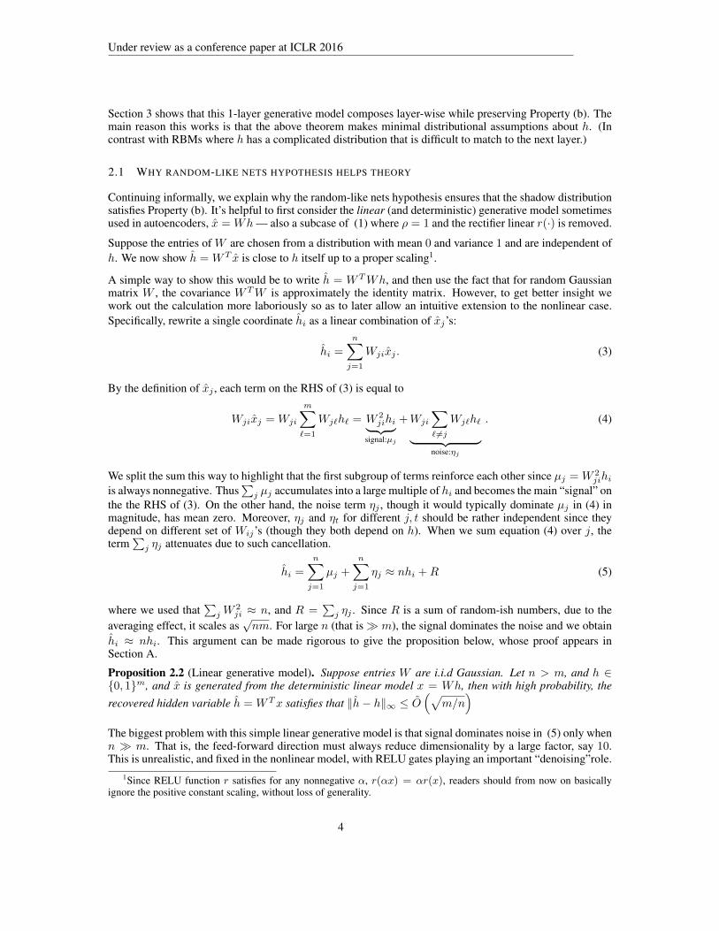
Section 3 shows that this 1-layer generative model composes layer-wise while preserving Property (b). Themain reason this works is that the above theorem makes minimal distributional assumptions about h. (Incontrast with RBMs where h has a complicated distribution that is difficult to match to the next layer.)

2.1 WHY RANDOM-LIKE NETS HYPOTHESIS HELPS THEORY

Continuing informally, we explain why the random-like nets hypothesis ensures that the shadow distributionsatisfies Property (b). It’s helpful to first consider the linear (and deterministic) generative model sometimesused in autoencoders, x = Wh — also a subcase of (1) where ρ = 1 and the rectifier linear r(·) is removed.

Suppose the entries of W are chosen from a distribution with mean 0 and variance 1 and are independent ofh. We now show h = WT x is close to h itself up to a proper scaling1.

A simple way to show this would be to write h = WTWh, and then use the fact that for random Gaussianmatrix W , the covariance WTW is approximately the identity matrix. However, to get better insight wework out the calculation more laboriously so as to later allow an intuitive extension to the nonlinear case.Specifically, rewrite a single coordinate hi as a linear combination of xj’s:

hi =

n∑j=1

Wjixj . (3)

By the definition of xj , each term on the RHS of (3) is equal to

Wjixj = Wji

m∑`=1

Wj`h` = W 2jihi︸︷︷︸

signal:µj

+Wji

∑` 6=j

Wj`h`︸︷︷︸noise:ηj

. (4)

We split the sum this way to highlight that the first subgroup of terms reinforce each other since µj = W 2jihi

is always nonnegative. Thus∑j µj accumulates into a large multiple of hi and becomes the main “signal” on

the the RHS of (3). On the other hand, the noise term ηj , though it would typically dominate µj in (4) inmagnitude, has mean zero. Moreover, ηj and ηt for different j, t should be rather independent since theydepend on different set of Wij’s (though they both depend on h). When we sum equation (4) over j, theterm

∑j ηj attenuates due to such cancellation.

hi =

n∑j=1

µj +

n∑j=1

ηj ≈ nhi +R (5)

where we used that∑jW

2ji ≈ n, and R =

∑j ηj . Since R is a sum of random-ish numbers, due to the

averaging effect, it scales as√nm. For large n (that is m), the signal dominates the noise and we obtain

hi ≈ nhi. This argument can be made rigorous to give the proposition below, whose proof appears inSection A.

Proposition 2.2 (Linear generative model). Suppose entries W are i.i.d Gaussian. Let n > m, and h ∈0, 1m, and x is generated from the deterministic linear model x = Wh, then with high probability, the

recovered hidden variable h = WTx satisfies that ‖h− h‖∞ ≤ O(√

m/n)

The biggest problem with this simple linear generative model is that signal dominates noise in (5) only whenn m. That is, the feed-forward direction must always reduce dimensionality by a large factor, say 10.This is unrealistic, and fixed in the nonlinear model, with RELU gates playing an important “denoising”role.

1Since RELU function r satisfies for any nonnegative α, r(αx) = αr(x), readers should from now on basicallyignore the positive constant scaling, without loss of generality.

4


2.2 Formal proof of Single-layer Reversibility

Now we give a formal version of Theorem 2.1. We begin by introducing a succinct notation for model (1),which will be helpful for later sections as well. Let t = ρn be the expected number of non-zeros in thevector ndrop, and let st(·) be the random function that drops coordinates with probability 1 − ρ, that is,st(z) = z ndrop. Then we rewrite model (1) as

x = st(r(αWh)) (6)

We make no assumptions on how large m and n are except to require that k < t. Since t is the (expected)number of non-zeros in vector x, it is roughly —up to logarithmic factor— the amount of “information”inx. Therefore the assumption that k < t is in accord with the usual “bottleneck” intuition, which says thatthe representation at higher levels has fewer bits of information.

The random-like net hypothesis here means that the entries of W independently satisfy Wij ∼ N (0, 1).

Wij ∼ N (0, 1) (7)

Also we assume the hidden variable h comes from any distribution Dh that is supported on nonnegative k-sparse vectors for some k, where none of the nonzero coordinates are very dominant. (Allowing a few largecoordinates wouldn’t kill the theory but the notation and math gets hairier.) Technically, when h ∼ Dh,

h ∈ Rn≥0, |h|0 ≤ k and |h|∞ ≤ β · ‖h‖ almost surely (8)

where β = O(√

(log k)/k ). The last assumption essentially says that all the coordinates of h shouldn’t betoo much larger than the average (which is 1/

√k · ‖h‖). As mentioned earlier the weak assumption on Dh

is the key to layerwise composability.Theorem 2.3 (Reversibility). Suppose t = ρn and k satisfy that k < t < k2. For (1 − n−5) measure ofW ’s, there exists offset vector b, such that the following holds: when h ∼ Dh and Pr[x|h] is specified bymodel (1), then with high probability over the choice of (h, x),

‖r(WTx+ b)− h‖2 ≤ O(k/t) · ‖h‖2, . (9)

The next theorem says that the generative model predicts that the trained net should be stable to dropout.Theorem 2.4 (Dropout Robustness). Under the condition of Theorem 2.3, suppose we further drop 1/2fraction of values of x randomly and obtain xdrop, then there exists some offset vector b′, such that with highprobability over the randomness of (h, xdrop), we have

‖r(2WTxdrop + b′)− h‖2 ≤ O(k/t) · ‖h‖2. (10)

To parse the theorems, we note that the error is on the order of the sparsity ratio k/t (up to logarithmic fac-tors), which is necessary since information theoretically the generative direction must increase the amountof information so that good inference is possible. In other words, our theorem shows that under our genera-tive model, feedforward calculation (with or without dropout) can estimate the hidden variable up to a smallerror when k t. Note that this is different from usual notions in generative models such as MAP or MLEinference. We get direct guarantees on the estimation error which neither MAP or MLE can guarantee2.

Furthermore, in Theorem 2.4, we need to choose a scaling of factor 2 to compensate the fact that half ofthe signal x was dropped. Moreover, we remark that an interesting feature of our theorems is that we showan almost uniform offset vector b (that is, b has almost the same entries across coordinate) is enough. Thismatches the observation that in the trained Alex net (Krizhevsky et al., 2012), for most of the layers theoffset vectors are almost uniform3. In our experiments (Section 4), we also found restricting the bias termsin RELU gates to all be some constant makes almost no change to the performance.

2Under the situation where MLE (or MAP) is close to the true h, our neural-net inference algorithm is also guaranteedto be the close to both MLE (or MAP) and the true h.

3Concretely, for the simple network we trained using implementation of (Jia et al., 2014), for 5 out of 7 hidden layers,the offset vector is almost uniform with mean to standard deviation ratio larger than 5. For layer 1, the ratio is about 1.5and for layer 3 the offset vector is almost 0.

5


We devote the rest of the sections to sketching a proof of Theorems 2.3 and 2.4. The main intermediate stepof the proof is the following lemma, which will be proved at the end of the section:Lemma 2.5. Under the same setting as Theorem 2.3, with high probability over the choice of h and x, wehave that for δ = O(1/

√t),

‖WTx− h‖∞ ≤ δ‖h‖ . (11)

Observe that since h is k-sparse, the average absolute value of the non-zero coordinates of h is τ = ‖h‖/√k.

Therefore the entry-wise error δ‖h‖ on RHS of (11) satisfies δ‖h‖ = ετ with ε = O(√k/t). This means

that WTh (the hidden state before offset and RELU) estimates the non-zeros of h with entry-wise relativeerror ε (in average), though the relative errors on the zero entries of h are huge. Therefore, even thoughwe get a good estimate of h in `∞ norm, the `2 norm of the difference WTx − h could be as large asετ√n = O(

√m/t)‖h‖ which could be larger than ‖h‖.

It turns out that the offset vector b and RELU have the denoising effects that reduce errors on the non-supportof h down to 0 and therefore drive the `2 error down significantly. The following proof of Theorem 2.3 (usingLemma 2.5) formalizes this intuition.

Proof of Theorem 2.3. Let h = WTx. By Lemma 2.5, we have that |hi − hi| ≤ δ‖h‖ for any i. Letb = −δ‖h‖. For any i with hi = 0, hi + b ≤ hi + δ‖h‖ + b ≤ 0, and therefore r(hi + b) = 0 = hi.On the other hand, for any i with hi 6= 0, we have |hi + b − hi| ≤ |b| + |hi − hi| ≤ 2δ‖h‖. It followsthat |r(hi + b) − r(hi)| ≤ 2δ‖h‖. Since hi is nonnegative, we have that |r(hi + b) − hi| ≤ 2δ‖h‖.Therefore the `2 distance between r(WTx + b) = r(h + b) and h can be bounded by ‖r(h + b) − h‖2 =∑i:hi 6=0 |r(hi + b)− hi|2 ≤ 4kδ2‖h‖2. Plugging in δ = O(1/

√t) we obtain the desired result.

Theorem 2.4 is a direct consequence of Theorem 2.3, essentially due to the dropout nature of our generativemodel (we sample in the generative model which connects to dropout naturally). See Section A for its proof.We conclude with a proof sketch of Lemma 2.5. The complete proof can be found in Section A.

Proof Sketch of Lemma 2.5. Here due to page limit, we give a high-level proof sketch that demonstrates thekey intuition behind the proof, by skipping most of the tedious parts. See section A for full details.

By a standard Markov argument, we claim that it suffices to show that w.h.p over the choice of ((W,h, x)the network is reversible, that is, Prx,h,W [equation (9) holds] ≥ 1 − n10 . Towards establishing this, wenote that equation (9) holds for any positive scaling of h, x simultaneously, since RELU has the propertythat r(βz) = β · r(z) for any β ≥ 0 and any z ∈ R. Therefore WLOG we can choose a proper scaling of hthat is convenient to us. We assume ‖h‖22 = k. By assumption (8), we have that |h|∞ ≤ O(

√log k).

Define h = αWTx. Similarly to (3), we fix i and expand the expression for hi by definition,

hi = α

n∑j=1

Wjixj (12)

Suppose ndrop has support T . Then we can write Wjixj as

Wjixj = Wjir(

m∑`=1

Wj`h`) · ndrop,j = Wjir(Wjihi + ηj) · 1j∈T , (13)

where ηj ,∑6=jWj`h`. Though r(·) is nonlinear, it is piece-wise linear and more importantly still

Lipschitz. Therefore intuitively, RHS of (13) can be “linearized” by approximating r(Wjihi+ηj) by 1ηj>0 ·(Wjihi + r(ηj)). Note that this approximation is not accurate only when |ηj | ≤ |Wjihi|, which happenswith relatively small probability, since ηj typically dominates Wjihi in magnitude.

Then Wjixj can be written approximately as 1ηj>0 ·(W 2jihi +Wjir(ηj)

), where the first term corresponds

to the bias and the second one corresponds to the noise (variance), similarly to the argument in the lineargenerative model case in Section 2.1.

6


x = sk0(r(α0W0h(1)))

h(`−1) = sk`−1(r(α`−1W`−1h

`))

h(1)

h(`)

W0

W`−1

(observed layer)

(a) Generative model

x

h(`−1)

h(1) = r(W T0 x + b1)

h(`) = r(W T`−1 + b`)

W T0

W T`−1

(observed layer)

(b) Feedforward NN

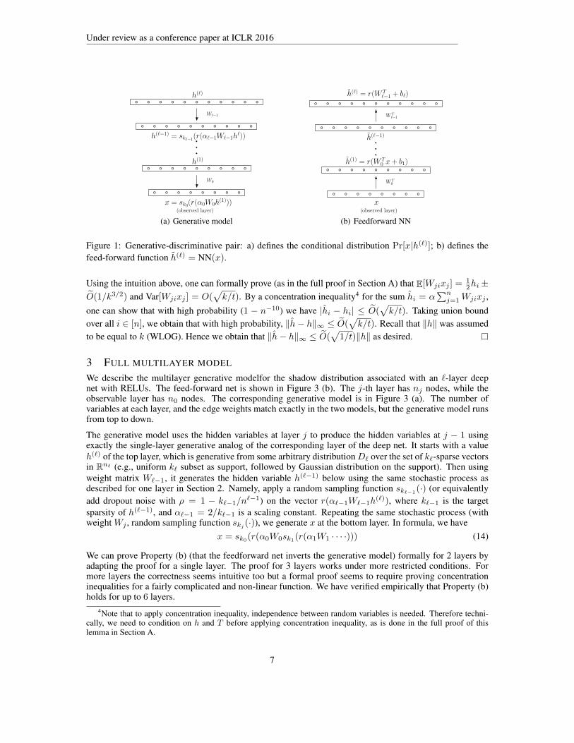
Figure 1: Generative-discriminative pair: a) defines the conditional distribution Pr[x|h(`)]; b) defines thefeed-forward function h(`) = NN(x).

Using the intuition above, one can formally prove (as in the full proof in Section A) that E[Wjixj ] = 12hi ±

O(1/k3/2) and Var[Wjixj ] = O(√k/t). By a concentration inequality4 for the sum hi = α

∑nj=1Wjixj ,

one can show that with high probability (1 − n−10) we have |hi − hi| ≤ O(√k/t). Taking union bound

over all i ∈ [n], we obtain that with high probability, ‖h− h‖∞ ≤ O(√k/t). Recall that ‖h‖ was assumed

to be equal to k (WLOG). Hence we obtain that ‖h− h‖∞ ≤ O(√

1/t)‖h‖ as desired.

3 FULL MULTILAYER MODEL

We describe the multilayer generative modelfor the shadow distribution associated with an `-layer deepnet with RELUs. The feed-forward net is shown in Figure 3 (b). The j-th layer has nj nodes, while theobservable layer has n0 nodes. The corresponding generative model is in Figure 3 (a). The number ofvariables at each layer, and the edge weights match exactly in the two models, but the generative model runsfrom top to down.

The generative model uses the hidden variables at layer j to produce the hidden variables at j − 1 usingexactly the single-layer generative analog of the corresponding layer of the deep net. It starts with a valueh(`) of the top layer, which is generative from some arbitrary distributionD` over the set of k`-sparse vectorsin Rn` (e.g., uniform k` subset as support, followed by Gaussian distribution on the support). Then usingweight matrix W`−1, it generates the hidden variable h(`−1) below using the same stochastic process asdescribed for one layer in Section 2. Namely, apply a random sampling function sk`−1

(·) (or equivalentlyadd dropout noise with ρ = 1 − k`−1/n

`−1) on the vector r(α`−1W`−1h(`)), where k`−1 is the target

sparsity of h(`−1), and α`−1 = 2/k`−1 is a scaling constant. Repeating the same stochastic process (withweight Wj , random sampling function skj (·)), we generate x at the bottom layer. In formula, we have

x = sk0(r(α0W0sk1(r(α1W1 · · · ·))) (14)

We can prove Property (b) (that the feedforward net inverts the generative model) formally for 2 layers byadapting the proof for a single layer. The proof for 3 layers works under more restricted conditions. Formore layers the correctness seems intuitive too but a formal proof seems to require proving concentrationinequalities for a fairly complicated and non-linear function. We have verified empirically that Property (b)holds for up to 6 layers.

4Note that to apply concentration inequality, independence between random variables is needed. Therefore techni-cally, we need to condition on h and T before applying concentration inequality, as is done in the full proof of thislemma in Section A.

7


We assume the random-like matrices Wj’s to have standard gaussian prior as in (7), that is,

Wj has i.i.d entries from N (0, 1) (15)

We also assume that the distributionD` produces k`-sparse vectors with not too large entries almost surely asin (8), that is, h(`) ∈ Rn`≥0 , |h(`)|0 ≤ k` and |h(`)|∞ ≤ O

(√logN/(k`)

)‖h‖ a.s. (Note thatN ,

∑j nj

is the total number of nodes in the architecture. )

Under this mathematical setup, we prove the following reversibility and dropout robustness results, whichare the 2-layers analog of Theorem 2.3 and Theorem 2.4.Theorem 3.1 (2-Layer Reversibility and Dropout Robustness). For ` = 2, and k2 < k1 < k0 < k22 , for0.9 measure of the weights (W0,W1), the following holds: There exists constant offset vector b0, b1 suchthat when h(2) ∼ D2 and Pr[x | h(2)] is specified as model (14), then network has reversibility and dropoutrobustness in the sense that the feedforward calculation (defined in Figure 3b) gives h(2) satisfying

∀i ∈ [n2], E[|h(2)i − h

(2)i |2

]≤ ετ2 (16)

where τ = 1k2

∑i h

(2)i is the average of the non-zero entries of h(2) and ε = O(k2/k1). Moreover, the

network also enjoys dropout robustness as in Theorem 2.4.

To parse the theorem, we note that when k2 k1 and k1 k0, in expectation, the entry-wise differencebetween h(2) and h(2) is dominated by the average single strength of h(2).

However, we note that we prove weaker results than in Theorem 2.3 – though the magnitudes of the error inboth Theorems are on the order of the ratio of the sparsities between two layers, here only the expectation ofthe error is bounded, while Theorem 2.3 is a high probability result. In general we believe high probabilitybounds hold for any constant layers networks, but seemingly proving that requires advanced tools for under-standing concentration properties of a complex non-linear function. Just to get a sense of the difficulties ofresults like Theorem 3.1, one can observe that to obtain h(2) from h(2) the network needs to be run twice inboth directions with RELU and sampling. This makes the dependency of h(2) on h(2) and W2 and W1 fairlycomplicated and non-linear.

Finally, we extend Theorem 3.1 to three layers with stronger assumptions on the sparsity of the top layer– We assume additionally that

√k3k2 < k0, which says that the top two layer is significantly sparser than

the bottom layer k0. We note that this assumption is still reasonable since in most of practical situations thetop layer consists of the labels and therefore is indeed much sparser. Weakening the assumption and gettinghigh probability bounds are left to future study.Theorem 3.2 (3-layers Reversibility and Dropout Robustness, informally stated). For ` = 3, when k3 <k2 < k1 < k0 < k22 and

√k3k2 < k0, the 3-layer generative model has the same type of reversibility and

dropout robustness properties as in Theorem 3.1.

4 EXPERIMENTS

We present experimental results that support our theory.

Verification of the random-like nets hypothesis. Testing the fully connected layers in a few trained net-works showed that the edge weights are indeed random-like. For instance Figure 4 in the appendix showsthe statistics for the the second fully connected layer in AlexNet (after 60 thousand training iterations). Edgeweights fit a Gaussian distribution, and bias in the RELU gates are essentially constant (in accord with The-orem 2.3) and the distribution of the singular values of the weight matrix is close to the quartercircular lawof random Gaussian matrices.

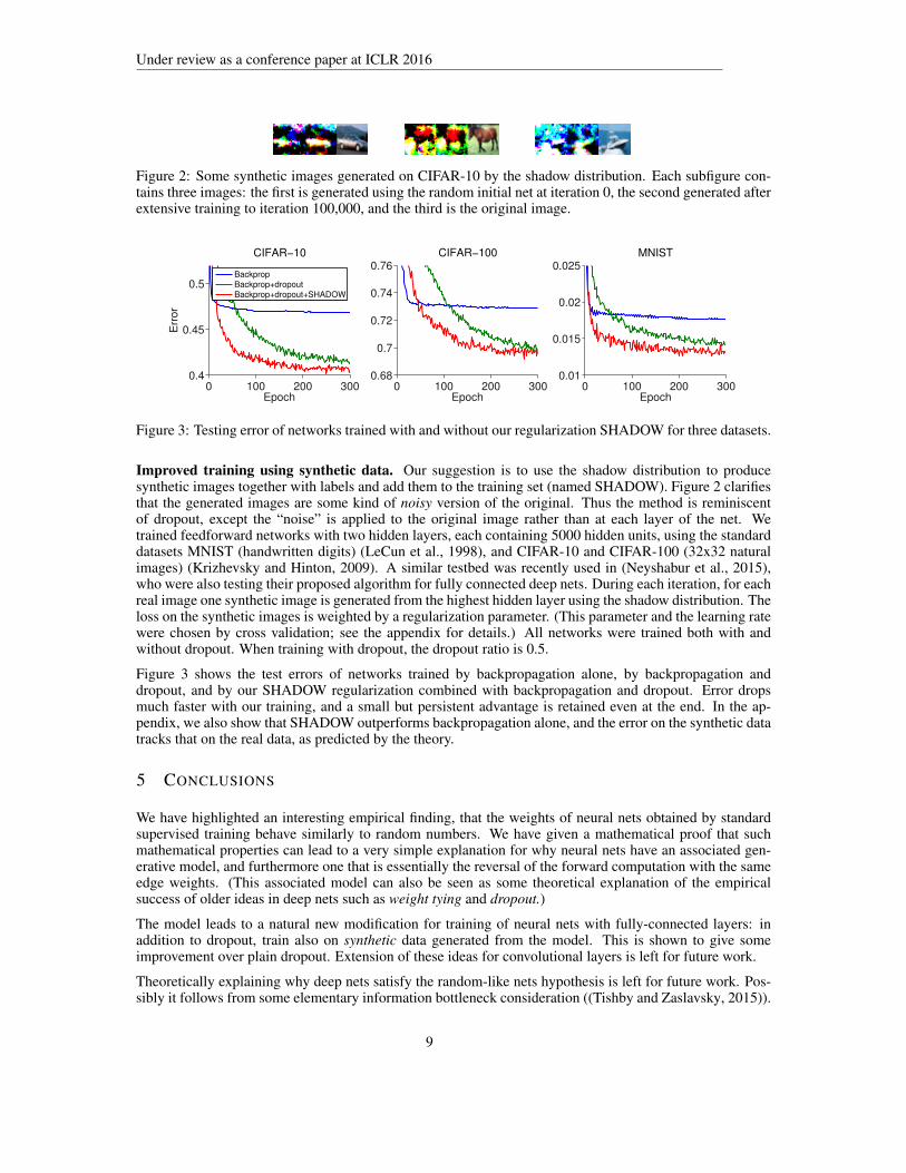
Generative model. We trained a 3-layer fully connected net on CIFAR-10 dataset as described below. Givenan image and a neural net our shadow distribution can be used to generate an image. Figure 2 shows thegenerated image using the initial (random) deep net, and from the trained net after 100,000 iterations.

8


Figure 2: Some synthetic images generated on CIFAR-10 by the shadow distribution. Each subfigure con-tains three images: the first is generated using the random initial net at iteration 0, the second generated afterextensive training to iteration 100,000, and the third is the original image.

0 100 200 3000.4

0.45

0.5

Epoch

Err

or

CIFAR−10

Backprop

Backprop+dropout

Backprop+dropout+SHADOW

0 100 200 3000.68

0.7

0.72

0.74

0.76

Epoch

CIFAR−100

0 100 200 3000.01

0.015

0.02

0.025

Epoch

MNIST

Figure 3: Testing error of networks trained with and without our regularization SHADOW for three datasets.

Improved training using synthetic data. Our suggestion is to use the shadow distribution to producesynthetic images together with labels and add them to the training set (named SHADOW). Figure 2 clarifiesthat the generated images are some kind of noisy version of the original. Thus the method is reminiscentof dropout, except the “noise” is applied to the original image rather than at each layer of the net. Wetrained feedforward networks with two hidden layers, each containing 5000 hidden units, using the standarddatasets MNIST (handwritten digits) (LeCun et al., 1998), and CIFAR-10 and CIFAR-100 (32x32 naturalimages) (Krizhevsky and Hinton, 2009). A similar testbed was recently used in (Neyshabur et al., 2015),who were also testing their proposed algorithm for fully connected deep nets. During each iteration, for eachreal image one synthetic image is generated from the highest hidden layer using the shadow distribution. Theloss on the synthetic images is weighted by a regularization parameter. (This parameter and the learning ratewere chosen by cross validation; see the appendix for details.) All networks were trained both with andwithout dropout. When training with dropout, the dropout ratio is 0.5.

Figure 3 shows the test errors of networks trained by backpropagation alone, by backpropagation anddropout, and by our SHADOW regularization combined with backpropagation and dropout. Error dropsmuch faster with our training, and a small but persistent advantage is retained even at the end. In the ap-pendix, we also show that SHADOW outperforms backpropagation alone, and the error on the synthetic datatracks that on the real data, as predicted by the theory.

5 CONCLUSIONS

We have highlighted an interesting empirical finding, that the weights of neural nets obtained by standardsupervised training behave similarly to random numbers. We have given a mathematical proof that suchmathematical properties can lead to a very simple explanation for why neural nets have an associated gen-erative model, and furthermore one that is essentially the reversal of the forward computation with the sameedge weights. (This associated model can also be seen as some theoretical explanation of the empiricalsuccess of older ideas in deep nets such as weight tying and dropout.)

The model leads to a natural new modification for training of neural nets with fully-connected layers: inaddition to dropout, train also on synthetic data generated from the model. This is shown to give someimprovement over plain dropout. Extension of these ideas for convolutional layers is left for future work.

Theoretically explaining why deep nets satisfy the random-like nets hypothesis is left for future work. Pos-sibly it follows from some elementary information bottleneck consideration ((Tishby and Zaslavsky, 2015)).

9


Another problem for future work is to design provably correct algorithms for deep learning assuming theinput is generated exactly according to our generative model. This could be a first step to deriving provableguarantees on backpropagation.

REFERENCES

Sanjeev Arora, Aditya Bhaskara, Rong Ge, and Tengyu Ma. Provable bounds for learning some deep representations.In Proceedings of the 31th International Conference on Machine Learning, ICML 2014, Beijing, China, 21-26 June2014, pages 584–592, 2014.

Yoshua Bengio. Learning deep architectures for AI. Foundations and Trends in Machine Learning, 2(1):1–127, 2009.

Yoshua Bengio, Pascal Lamblin, Dan Popovici, and Hugo Larochelle. Greedy layer-wise training of deep networks. InNIPS, pages 153–160, 2006.

Yoshua Bengio, Eric Thibodeau-Laufer, Guillaume Alain, and Jason Yosinski. Deep generative stochastic networkstrainable by backprop. arXiv preprint arXiv:1306.1091, 2013a.

Yoshua Bengio, Li Yao, Guillaume Alain, and Pascal Vincent. Generalized denoising auto-encoders as generativemodels. In Advances in Neural Information Processing Systems, pages 899–907, 2013b.

Yoav Freund and David Haussler. Unsupervised learning of distributions on binary vectors using two layer networks.Technical report, 1994.

Ian J. Goodfellow, Jean Pouget-Abadie, Mehdi Mirza, Bing Xu, David Warde-Farley, Sherjil Ozair, Aaron C. Courville,and Yoshua Bengio. Generative adversarial nets. In Advances in Neural Information Processing Systems 27: AnnualConference on Neural Information Processing Systems 2014, December 8-13 2014, Montreal, Quebec, Canada, pages2672–2680, 2014. URL http://papers.nips.cc/paper/5423-generative-adversarial-nets.

Geoffrey E Hinton and Ruslan R Salakhutdinov. Reducing the dimensionality of data with neural networks. Science,313(5786):504–507, 2006.

Geoffrey E. Hinton, Simon Osindero, and Yee Whye Teh. A fast learning algorithm for deep belief nets. NeuralComputation, 18(7):1527–1554, 2006.

Yangqing Jia, Evan Shelhamer, Jeff Donahue, Sergey Karayev, Jonathan Long, Ross Girshick, Sergio Guadarrama, andTrevor Darrell. Caffe: Convolutional architecture for fast feature embedding. arXiv preprint arXiv:1408.5093, 2014.

Diederik P. Kingma, Shakir Mohamed, Danilo Jimenez Rezende, and Max Welling. Semi-supervised learning with deepgenerative models. In NIPS, pages 3581–3589, 2014.

Alex Krizhevsky and Geoffrey Hinton. Learning multiple layers of features from tiny images. Computer ScienceDepartment, University of Toronto, Tech. Rep, 1(4):7, 2009.

Alex Krizhevsky, Ilya Sutskever, and Geoff Hinton. Imagenet classification with deep convolutional neural networks. InAdvances in Neural Information Processing Systems 25, pages 1106–1114. 2012.

Guillaume Lecue. Lecutre notes on basic tools from empirical processes theory applied to compress sensing problem.2009.

Yann LeCun, Leon Bottou, Yoshua Bengio, and Patrick Haffner. Gradient-based learning applied to document recogni-tion. Proceedings of the IEEE, 86(11):2278–2324, 1998.

Honglak Lee, Roger Grosse, Rajesh Ranganath, and Andrew Y. Ng. Convolutional deep belief networks for scalableunsupervised learning of hierarchical representations. In ICML, ICML ’09, pages 609–616, New York, NY, USA,2009a. ACM. ISBN 978-1-60558-516-1. doi: 10.1145/1553374.1553453. URL http://doi.acm.org/10.1145/1553374.1553453.

Honglak Lee, Roger Grosse, Rajesh Ranganath, and Andrew Y Ng. Convolutional deep belief networks for scalableunsupervised learning of hierarchical representations. In Proceedings of the 26th Annual International Conferenceon Machine Learning, pages 609–616. ACM, 2009b.

10

http://papers.nips.cc/paper/5423-generative-adversarial-nets

http://doi.acm.org/10.1145/1553374.1553453

http://doi.acm.org/10.1145/1553374.1553453


A. Mahendran and A. Vedaldi. Understanding deep image representations by inverting them. In IEEE Conference onComputer Vision and Pattern Recognition, 2015.

Vinod Nair and Geoffrey E Hinton. Rectified linear units improve restricted boltzmann machines. In Proceedings of the27th International Conference on Machine Learning (ICML-10), pages 807–814, 2010.

Behnam Neyshabur, Ruslan Salakhutdinov, and Nathan Srebro. Path-sgd: Path-normalized optimization in deep neuralnetworks. In NIPS, 2015.

Andrew Y. Ng and Michael I. Jordan. On discriminative vs. generative classifiers: A comparison of logistic regressionand naive bayes. In Advances in Neural Information Processing Systems 14 [Neural Information Processing Systems:Natural and Synthetic, NIPS 2001, December 3-8, 2001, Vancouver, British Columbia, Canada], pages 841–848,2001.

A. B. Patel, T. Nguyen, and R. G. Baraniuk. A Probabilistic Theory of Deep Learning. ArXiv e-prints, 2015.

Rajesh Ranganath, Linpeng Tang, Laurent Charlin, and David M. Blei. Deep exponential families. In AISTATS, 2015.

N. Tishby and N. Zaslavsky. Deep Learning and the Information Bottleneck Principle. ArXiv e-prints, March 2015.

Pascal Vincent, Hugo Larochelle, Yoshua Bengio, and Pierre-Antoine Manzagol. Extracting and composing robustfeatures with denoising autoencoders. In ICML, pages 1096–1103, 2008.

Pascal Vincent, Hugo Larochelle, Isabelle Lajoie, Yoshua Bengio, and Pierre-Antoine Manzagol. Stacked denoisingautoencoders: Learning useful representations in a deep network with a local denoising criterion. The Journal ofMachine Learning Research, 11:3371–3408, 2010.

11


APPENDIX

A COMPLETE PROOFS FOR ONE-LAYER REVERSIBILITY

Proof of Lemma 2.5. We claim that it suffices to show that w.h.p5 over the choice of ((W,h, x) the networkis reversible (that is, (9) holds),

Prx,h,W

[equation (9) holds] ≥ 1− n10 . (17)

Indeed, suppose (17) is true, then using a standard Markov argument, we obtain

PrW

[Prx,h

[equation (9) holds |W ] > 1− n−5]≥ 1− n5,

as desired.

Now we establish (17). Note that equation (9) (and consequently statement (17)) holds for any positivescaling of h, x simultaneously, since RELU has the property that r(βz) = β · r(z) for any β ≥ 0 and anyz ∈ R. Therefore WLOG we can choose a proper scaling of h that is convenient to us. We assume ‖h‖22 = k.By assumption (8), we have that |h|∞ ≤ O(

√log k).

Define h = αWTx. Similarly to (3), we fix i and expand the expression for hi by definition and obtainhi = α

∑nj=1Wjixj . Suppose ndrop has support T . Then we can write xj as

xj = r(

m∑`=1

Wj`h`) · ndrop,j = r(Wjihi + ηj) · 1j∈T , (18)

where ηj ,∑` 6=jWj`h`. Though r(·) is nonlinear, it is piece-wise linear and more importantly still

Lipschitz. Therefore intuitively, RHS of (18) can be “linearized” by approximating r(Wjihi+ηj) by 1ηj>0 ·(Wjihi + r(ηj)). Note that this approximation is not accurate only when |ηj | ≤ |Wjihi|, which happenswith relatively small probability, since ηj typically dominates Wjihi in magnitude.

Using the intuition above, we can formally calculate the expectation ofWjixj via a slightly tighter and moresophisticated argument: Conditioned on h, we have Wji ∼ N (0, 1) and ηj =

∑` 6=jWj`h` ∼ N (0, σ2)

with σ2 = ‖h‖2 − h2j = k − h2j ≥ Ω(k). Therefore we have log σ = 12 log(Ω(k)) ≥ hj and then by

Lemma B.1 (Wji here corresponds to w in Lemma B.1, ηj to ξ and hj to h), we have E[Wjixj | h] =

E[Wjir(Wjihj + ηj) | h] = 12hi ± O(1/k3/2).

It follows that

E[hi|h, T ] =∑j∈T

E[Wjir(Wjihj + ηj) | h] =α|T |

2hi ± O(αt/k3/2)

Taking expectation over the choice of T we obtain that

E[hi|h] =αt

2hi ± O(αn/k3/2) = hi ± O(1/(k3/2)) (19)

. (Recall that t = ρn and α = 2/(ρn). Similarly, the variance of hi|h can be bounded by Var[hi|h] = O(k/t)

(see Claim A.2). Therefore we expect that hi concentrate around its mean with fluctuation ±O(√k/t).

Indeed, by by concentration inequality, we can prove (see Lemma A.1 in Section A) that actually hi | his sub-Gaussian, and therefore conditioned on h, with high probability (1 − n−10) we have |hi − hi| ≤

5We use w.h.p as a shorthand for “with high probability” in the rest of the paper.

12


O((√k/t+1/k3/2), where the first term account for the variance and the second is due to the bias (difference

between E[hi] and hi).

Noting that k < t < k2 and therefore 1/k3/2 is dominated by√k/t, take expectation over h, we obtain

that Pr[|hi − hi| ≥ Ω(

√k/t)

]≤ n−10. Taking union bound over all i ∈ [n], we obtain that with high

probability, ‖h − h‖∞ ≤ O(√k/t). Recall that ‖h‖ was assumed to be equal k without loss of generality.

Hence we obtain that ‖h− h‖∞ ≤ O(√

1/t)‖h‖ as desired.

Proof of Theorem 2.4. Recall that in the generative model already many bits are dropped, and neverthe-less the feedforward direction maps it back to h. Thus dropping some more bits in x doesn’t make muchdifference. Concretely, we note that xdrop has the same distribution as st/2(r(αWh)). Therefore invokingTheorem 2.3 with t being replaced by t/2, we obtain that there exists b′ such that ‖r(2WTxdrop +b′)−h‖2 ≤O(k/t) · ‖h‖.

Lemma A.1. Under the same setting as Theorem 2.3, let h = αWTh. Then we have

Pr[|hi − hi| ≥ Ω((

√k/t+ 1/k3/2) | h

]≤ n−10

Proof of Lemma A.1. Recall that hi =∑j∈T αWjir(Wjihj + ηj). For convenience of notation, we condi-

tion on the randomness h and T and only consider the randomness ofW implicitly and omit the conditioningnotation. Let Zj be the random variable αWjixj = αWjir(Wjihj + ηj). Therefore Zj are independentrandom variables (conditioned on h and T ). Our plan is to show that Zj has bounded Orlicz norm andtherefore hi =

∑j Zj concentrates around its mean.

SinceWji and xj are Gaussian random variables with variance 1 and ‖h‖ =√k, we have that ‖Wji‖ψ2

= 1

and ‖xj‖ψ2≤√k. This implies that Wjixj is sub-exponential random variables, that is, ‖Wjixj‖ψ1

≤O(√k). That is, Zj has ψ1 orlicz norm at most O(α

√k). Moreover by Lemma D.2, we have that

‖Zj −E[Zj ]‖ψ1≤ O(α

√k). Then we are ready to apply bernstein inequalities for sub-exponential random

variables (Theorem D.1) and obtain that for some universal constant c,

Pr

∣∣∣∣∣∣∑j∈T

Zj − E

∑j∈T

Zj

∣∣∣∣∣∣ > c√|T |α√k log n

≤ n−10 .Equivalently, w obtain that

Pr[∣∣∣hi − E

[hi

]∣∣∣ > c√|T |k/t2 log n | h, T

]≤ n−10 .

Note that with high probability, |T | = (1 ± o(1))t. Therefore taking expectation over T and taking unionbound over i ∈ [n] we obtain that for some absolute constant c,

Pr[∀i ∈ [n],

∣∣∣hi − E[hi

]∣∣∣ > c√k/t log n | h

]≤ n−8 .

Finally note that as shown in the proof of Theorem 2.3, we have E[hi | h] = hi ± 1/k3/2. Combining withthe equation above we get the desired result.

13


Claim A.2. Under the same setting as in the proof of Theorem 2.3. The variance of hi can be bounded by

Var[hi|h] ≤ O(k/t)

Proof. Using Cauchy-Schwartz inequality we obtain

Var[Wjixj |h] ≤ E[W 2jixj ]

2|h]

≤ E[W 4ji|h]1/2 E[x4j |h]1/2 ≤ O(k)

It follows that

Var[hi|h] = ET

∑j∈T

α2Var[Wjixj |h]

≤ α2t ·O(k) = O(k/t),

We note that a tighter calculation of the variance can be obtained using Lemma B.1).

B AUXILIARY LEMMAS FOR ONE LAYER MODEL

We need a series of lemmas for the one layer model, which will be further used in the proof of two layersand three layers result.

As argued earlier, the particular scaling of the distribution of h is not important, and we can assume WLOGthat ‖h‖2 = k. Throughout this section, we assume that for h ∼ Dh,

h ∈ Rn≥0, |h|0 ≤ k , ‖h‖ = k , and |h|∞ ≤ O(√

logN) almost surely (20)

Lemma B.1. Suppose w ∈ N (0, 1) and ξ ∼ N (0, σ2) are two independent variables. For σ = Ω(1) and0 ≤ h ≤ log(σ), we have that E [w · r(wh+ ξ)] = h

2 ± O(1/σ3) and E[w2 · r(wh+ ξ)2] ≤ 3h2 + σ2.

Proof. Let φ(x) = 1σ√2π

exp(− x2

2σ2 ) be the density function for random variable ξ. Let C1 = E[|ξ|/σ] =2σ

∫∞0φ(x)xdx. We start by calculating E [r(wh+ ξ) | w] as follows:

E [w · r(wh+ ξ) | w] = w

∫ ∞−wh

φ(x)(wh+ x)dx

= w

∫ ∞0

φ(x)(wh+ x)dx+ w

∫ 0

−whφ(x)(wh+ x)dx

=C1σw

2+w2h

2+ w

∫ wh

0

φ(y)(wh− y)dy︸︷︷︸G(w)

Therefore we have that

E [E [w · r(wh+ ξ) | w]] =h

2+ E[G(w)]

Thus it remains to understand G(w) and bound its expectation. We calculate the derivative of G(w): Wehave that G(w) can be written as

14


G(w) = w2h

∫ wh

0

φ(y)dy − w∫ wh

0

φ(y)ydy

and its derivative is

G(w)′ = 2wh

∫ wh

0

φ(y)dy + w2h2φ(wh)−∫ wh

0

φ(y)ydy − w2h2φ(wh)

= 2wh

∫ wh

0

φ(y)dy −∫ wh

0

φ(y)ydy

The it follows that

G(w)′′ = 2h

∫ wh

0

φ(y)dy + 2wh2φ(wh)− wh2φ(wh)

= 2h

∫ wh

0

φ(y)dy + wh2φ(wh)

Moreover, we can get the third derivative and forth oneG(w)′′′ = 3h2φ(wh) + wh3φ′(wh)

andG(w)(4) = 4h3φ′(wh) + wh4φ′′(wh)

Therefore for h ≤ 10 log(σ) and w with |w| ≤ 10 log(σ), using the fact that φ′(wh) =1

σ√2π

exp(−w2h2

2σ2 )whσ2 ≤ 2whσ3√2π

and similarly, φ′′(wh) ≤ 1σ3√2π

. It follows that G(w)(4) ≤ O(wh4

σ3 )

for any w ≤ 10 log(σ).

Now we are ready to bound E[G(w)]: By Taylor expansion at point 0, we have that G(w) = h2φ(0)2 w3 +

G(ζ)(4)

24 w4 for some ζ between 0 and w. It follows that for |w| ≤ 10 log(σ), |G(w)− h2φ(0)2 w3| ≤ O(1/σ3),

and therefore we obtain that∣∣∣∣E [G(w) | |w| ≤ 10 log σ]− E[h2φ(0)

2w3 | |w| ≤ 10 log σ

]∣∣∣∣ ≤ E[∣∣∣∣G(w)− h2φ(0)

2w3

∣∣∣∣ | |w| ≤ 10 log σ

]≤ O(1/σ3)

Since w||w| ≤ 10 log σ is symmetric, we have E[h2φ(0)

2 w3 | |w| ≤ 10 log σ]

= 0, and it follows that

E[G(w) | |w| ≤ 10 log σ] ≤ O(1/σ3). Moreover, note that |G(w)| ≤ O(w3h2) ≤ O(log2 σw3), then wehave that

E[G(w) | |w| ≥ 10 log σ] Pr[|w| ≥ 10 log σ] ≤ σ−4∫|w|≥10 log σ

O(log2 σw3) exp(−w2/2)dw ≤ O(1/σ3)

Therefore altogether we obtain

E[G(w)] = E[G(w) | |w| ≥ 10 log σ] Pr[|w| ≥ 10 log σ] + E[G(w) | |w| ≤ 10 log σ] Pr[|w| ≤ 10 log σ]

= O(1/σ3) +O(1/σ3) = O(1/σ3).

Finally we bound the variance of w · r(wh+ ξ). We have that

E[w2 · r(wh+ ξ)2] ≤ E[w2 · (wh+ ξ)2] = h2 E[w4] + E[w2]E[ξ2] = 3h2 + σ2 .

as desired.

15


Lemma B.2. For any a, b ≥ 0 with a, b ≤ 5 log σ and random variable u, v ∼ N (0, 1) and ξ ∈ N (0, σ2),we have that

∣∣E[uv · r(au+ bv + ξ)2]− E[ur(au+ bv + ξ)]E[vr(au+ bv + ξ)]∣∣ = O(1).

Proof. Let t =√a2 + b2 in this proof. We first represent u = 1

t (ax + by) and v = 1t (bx − ay), where

x = 1t (au+ bv) and y = 1

t (bu− av) are two independent Gaussian random variables drawn fromN (0, 1).We replace u, v by the new parameterization,

E[uv · r(au+ bv + ξ)2] = E[

1

t2(ax+ by)(bx− ay)r(tx+ ξ)2

]= E

[1

t2abx2r(tx+ ξ)2

]− E

[1

t2abr(tx+ ξ)2

]= E

[1

t2ab(x2 − 1)r(tx+ ξ)2

]where we used the fact that E[y] = 0 and y is independent with x and ξ.

Then we expand the expectation by conditioning on x and taking expectation over ξ:

(x2 − 1)E[r(tx+ ξ)2 | x] = (x2 − 1)

∫ ∞−tx

(tx+ y)2φ(y)dy

= (x2 − 1)

∫ 0

−tx(tx+ y)2φ(y)dy + (x2 − 1)

∫ ∞0

(tx+ y)2φ(y)dy

= (x2 − 1)

∫ tx

0

(tx− y)2φ(y)dy + (x2 − 1)(C0t2x2 + 2C1tx+ C2)

, H(x) + (x2 − 1)(C0t2x2 + 2C1tx+ C2)

where C0 =∫∞0φ(y)dy = 1

2 , and C1, C2 are two other constants (the values of which we don’t care) thatdon’t depend on x. Therefore by Lemma B.3, we obtain that |E[H(x)]| ≤ O(1/σ) and therefore takingexpectation of the equation above we obtain that

E[(x2 − 1)E[r(tx+ ξ)2 | x]] = E[H(x)] + E[(x2 − 1)(C2t2x2 + 2C1tx+ C0)]

= 2C2t2 ± O(1/σ) = t2 ± O(1/σ)

Therefore we have that E[uv · r(au+ bv+ ξ)2] = E[1t2 ab(x

2 − 1)r(tx+ ξ)2]

= O(1). Using the fact that

E[ur(au+ bv + ξ)] ≤ O(1) and E[vr(au+ bv + ξ)] ≤ O(1), we obtain that∣∣E[uv · r(au+ bv + ξ)2]− E[ur(au+ bv + ξ)]E[vr(au+ bv + ξ)]∣∣ = O(1).

Lemma B.3. Suppose z ∼ N (0, 1), and let φ(x) = 1σ√2π

exp(− x2

2σ2 ) be the density function of N (0, σ2)

where σ = Ω(1). For r ≤ 10 log σ, define G(z) =∫ rz0

(rz − y)2φ(y)dy, and H(z) = (z2 − 1)G(z). Thenwe have that E[|H(z)|] ≤ O(1/σ)

Proof. Our technique is to approximate H(z) using taylor expansion at point close to 0, and then argue thatsince z is very unlikely to be very large, so the contribution of large z is negligible. We calculate the derivate

16


of H at point z as follows:H(z)′ = 2zG(z) + (z2 − 1)G′(z)

H(z)′′ = 2G(z) + 4zG′(z) + (z2 − 1)G′′(z)

H(z)′′′ = 6G′(z) + 6zG′′(z) + (z2 − 1)G′′′(z)

Moreover, we have that the derivatives of G

G′(z) =

∫ rz

0

2r(rz − y)φ(y)dy

G′′(z) =

∫ rz

0

2r2φ(y)dy

G′′′(z) = 2r3φ(rz)

Therefore we have that G′(0) = G′′(0) = 0 and H ′(0) = H ′′(0) = 0. Moreover, when r ≤ 10 log σ

and z ≤ 10 log σ and we have that bound that |H ′′′(z)| ≤ O(1/σ). Therefore, we have that for z ≤10 log σ, |H(z)| ≤ O(1/σ), and therefore we obtain that E[H(z) | |z| ≤ 10 log σ] Pr[|z| ≤ 10 log σ] ≤O(1/σ). Since |H(z)| ≤ O(1) · z4 for any z, we obtain that for z ≥ 10 log σ, the contribution is negligible:E[H(z) | |z| > 10 log σ] Pr[|z| > 10 log σ] ≤ O(1/σ2). Therefore altogether we obtain that |E[|H(z)|]| ≤O(1/σ).

The following two lemmas are not used for the proof of single layer net, though they will be useful forproving the result for 2-layer net. The following lemma bound the correlation between hi and hj .

Lemma B.4. Let h = WTx, andDh satsifies (20), then for any i, j, we have that |E[hihj ]−E[hi]E[hj ]| ≤O(1/t).

Proof. We expand the definition of hi and hj directly.

E[hihj ] = α2 E

[(∑u∈S

Wuixu

)(∑v∈S

Wvjxv

)]= α2

∑u∈S

E[WuiWvix

2u

]+ α2

∑u 6=v

E [WuiWvjxuxv]

= α2∑u∈S

E[WuiWvix

2u

]+ α2

∑u 6=v

E [Wuixu]E [Wvjxuxv]

= α2∑u∈S

(E[WuiWvix

2u

]− E[Wuixu]E[Wvjxv]

)+ α2

∑u,v

E [Wuixu]E [Wvjxuxv]

= α2∑u∈S

(E[WuiWvix

2u


)+ E[hi]E[hj ]

where in the third line we use the fact that Wuixu is independent with Wvjxv , and others are basic algebramanipulation. Using Lemma B.4, we have that∣∣E [WuiWvix

2u


∣∣ ≤ O(1)

Therefore we obtain that ∣∣∣E[hihj ]− E[hi]E[hj ]∣∣∣ = α2O(t) = O(1/t)

17


The following lemmas shows that theLemma B.5. Under the single-layer setting of Lemma B.4, let K be the support of h. Then for any k-dimensional vector uK such that |uK |∞ ≤ O(1), we have that

E[|uTK(hK − E hK)|2] ≤ O(k2/t)

Proof. We expand our target and obtain,

E[|uTK(hK − EhK)|2] = E[|∑i∈K

ui(hi − Ehi)|2]

=∑i∈K

E[u2i (hi − Ehi)2] + E

∑i6=j

uiuj(hi − Ehi)(hj − Ehj)

=∑i∈K

E[(hi − Ehi)2] · O(1) + maxi 6=j|E[hihj ]− E[hi]E[hj ]| · O(1) · k2

By Lemma A.2, we have that E[(hi − Ehi)2] ≤ O(‖h‖2/t). By Lemma B.4, therefore we obtain thatmaxi6=j|E[hihj ]− E[hi]E[hj ]| ≤ O(1/t). Using the fact that ‖h‖2 ≤ O(k),

E[|uTK(hK − EhK)|2] ≤ O(k2/t)

C MULTILAYER REVERSIBILITY AND DROPOUT ROBUSTNESS

We state the formal version of Theorem 3.1 here. Recall that we assume the distribution of h(`) satisfies that

h(`) ∈ Rn`≥0 , |h(`)|0 ≤ k` and |h(`)|∞ ≤ O(√

logN/(k`))‖h‖ a.s. (21)

Theorem C.1 (2-Layer Reversibility and Dropout Robustness). For ` = 2, and k2 < k1 < k0 < k22 , thereexists constant offset vector b0, b1 such that with probability .9 over the randomness of the weights (W0,W1)from prior (15), and h(2) ∼ D2 that satisfies (21), and observable x generated from the 2-layer generativemodel (14), the hidden representations obtained from running the network feedforwardly

h(1) = r(WT0 x+ b1), and h(2) = r(WT

1 h(1) + b2)

are entry-wise close to the original hidden variables

∀i ∈ [n2], E[|h(2)i − h

(2)i |2

]≤ O(k2/k1) · h(2) (22)

∀i ∈ [n1], E[|h(1)i − h

(1)i |2

]≤ O(k1/k0) · h(1) (23)

where h(2) = 1k2

∑i h

(2)i and h(1) = 1

k1

∑i h

(1)i are the average of the non-zero entries of h(2) and h(1).

Moreover, there exists offset vector b′1 and b′2, such that when hidden representation is calculated feedfor-wardly with dropping out a random subset G0 of size n0/2 in the observable layer and G2 of size n1/2 inthe first hidden layer:

h(1)drop = r(2WT0 (x n0drop) + b′1), and h(2) = r(2WT

1 (h(1) n1drop) + b′2)

are entry-wise close to the original hidden variables in the same form as equation (22) and (23). (Heren0drop and n1drop are uniform random binary vector of size n0 and n1, which governs which coordinates to bedropped).

18


For the ease of math, we use a cleaner notation and setup as in Section 3. Suppose there are two hidden layersg ∈ Rp and h ∈ Rm and one observable layer x. We assume the sparsity of top layer is q,and we assume inour generative model that h = sk(r(βUg)) and x = st(r(αWh)) where U and W are two random matriceswith standard normal entries.

Let h = r(WTx + b) and g = r(UTh + c), where b and c two offset vectors. Our result in the last sectionshow that h ≈ h, and in the section we are going to show g ≈ g. The main difficulty here is that the value ofh and h depends on the randomness of U and therefore the additional dependency and correlation introducedmakes us hard to write g as a linear combination of independent variables. Here we aim for a weaker resultand basically prove that E[|gr − gr|2] is small for any index r ∈ [p].Theorem C.2. When q < k < t < q2, and any fixed g ∈ Rp with |g|0 ≤ q and ‖g‖2 = Θ(

√q) and

|g|∞ ≤ O(1), for α = 2t , β = 2/k and some b, and c, with high probability over the randomness of W , g

satisfies that for any r ∈ [p],E[‖gr − gr‖2] ≤ O(q/k)

Proof. We fix an index r ∈ [p], and consider gr and gr. Moreover, we fix the choice of random samplingfunction sk(·) and st(·) to the function sk(x) = [xK , 0] and st(x) = [xT , 0], where K and T be subsets of[m] and [n], with size k and t, respectively. Let gr = UTr h where Ur is the r-th column of U , that is, gr isthe version before shift and rectifier linear. Further more, let’s assume UTr = uT = [u1, . . . , um] and uK isthe its restriction to subset K. Therefore, gr can be written as

gr = uT h = uTh+ uT (h− h) (24)

By Lemma 2.5 (applying to the layer between g and h), we know that with high probability over the ran-domness of U , |uTh − gr| ≤ O

(√q/k)

. We conditioned on the event E that |uTh − gr| ≤ O(√

q/k)

,

and that ‖u‖∞ ≤ O(1) in the rest of the proof (note that event E happens with high probability).

Now it suffices to prove that uT (h − h) is small. First of all, we note that with high probability over therandomness of W , h matches h on the support, therefore we can write uT (h− h) = uTK(hK − hK), whichturns out to be essential for bounding the error. We further decompose it into

uTK(hK − hK) = uTK(hK − E[hK ]) + uTK(E[hK ]− hK) + uT (hK − hK), (25)

and bound them individually.

First of all, we note that hi is typically of magnitude β√q where q is the sparsity of g,and ‖h‖ ≈ β

√kq.

We first scale down h by β√q and then h/(β

√q) meets the scaling of equation (20). We are going to apply

Lemmas in Section B with h/(β√q).

by equation 19, we have that |E[hi]/(β√q)− hi/(β√q)| ≤ O(1/(q3/2)), and therefore |E[hK ]− hK |1 ≤

O(β√q · 1/(q3/2k) · k) = O(1/q).

Therefore uTK(hK −E[hK ]) ≤ |u|∞|E[hK ]−hK |1 ≤ O(1/q). Moreover, we note that hK − hK = b1K isa constant vector and therefore uT (hK − hK) = b′ for a constant b (which depends on r and u implicitly).

Finally we bound the term uTK(hK − E[hK ]). We invoke Lemma B.5 (with h/(β√q)) and obtain that

‖E[|uTK(hK/(β√q)− E[hK ]/(β

√q))|2 | h, E ]‖ ≤ O(k2/t)

It follows that‖E[|uTK(hK − E[hK ])|2 | h, E ]‖ ≤ O(q/t)

Note that the small probability event has only negligible contribution to the the expectation, therefore bound-ing the difference and marginalize over h, we obtain that E[‖uTK(hK − E[hK ])‖2] ≤ O(q/t). Therefore we

19


have bounded the three terms in RHS of (25). E[|gr − uT h|2] ≤ O(1/q + q/k) = O(q/k). Note thatg = r(g + b), therefore for any b = ε1 with ε ≤ O(q/k), we obtain that E

[‖g − g‖2∞

]≤ O(q/k).

C.1 PROOF SKETCH OF THEOREM 3.2

As argued in Section 3, the drawback of not getting high probability bound in the 2-layer Theorems is thatwe lose the denoising property of rectifier linear. Note that since |gr − gr| is only small in expectation,passing through the rectifier linear we obtain r(g+ c), and we can’t argue that r(g+ c) matches the supportg theoretically. (Though experimentally and intuitively, we believe that choosing c to be proportional to thenoise would remove the noise on all the non-support of g. )

However, bounding the error in a weaker way we could obtain Theorem 3.2. The key idea is that the in athree layer network described as in Section 3, the inference error of h(3) come from three sources: the errorcaused caused by incorrectly recover h(1), h(2) and the error of reversing the third layer W2. The later twosources error reduces to two and one layer situation and therefore we can bound them. For the first sourceof error, we note that by Theorem C.2, the

D TOOLBOX

Definition 1 (Orlicz norm ‖ · ‖ψα ). For 1 ≤ α < ∞, let ψα(x) = exp(xα) − 1. For 0 < α < 1, letψα(x) = xα − 1 for large enough x ≥ xα, and ψα is linear in [0, xα]. Therefore ψα is convex. The Orlicznorm ψα or a random variable X is defined as

‖X‖ψα , infc ∈ (0,∞) | E [ψα(|X|/c) ≤ 1] (26)

Theorem D.1 (Bernstein’ inequality for subexponential random variables (Lecue, 2009)). There exists anabsolute constant c > 0 for which the following holds: Let X1, . . . , Xn be n independent mena zero ψ1

random variables. Then for every t > 0,

Pr

[∣∣∣∣∣n∑i=1

Xi

∣∣∣∣∣ > t

]≤ 2 exp

(−cmin

(t2

nv,t

M

))where M = maxi ‖Xi‖ψ1

and v = n−1∑i ‖Xi‖2ψ1

.

Lemma D.2. Suppose random variable X has ψα orlicz norm a, then X − E[X] has ψα orlicz norm atmost 2a.

Proof. First of all, since ψα is convex and increasing on [0,∞), we have that E [ψα(|X|/a)] ≥ψα(E[|X|]/a) ≥ ψα(|E[X]|/a). Then we have that

E[ψα(|X − EX|

2a)

]≤ E[ψα(

|X|2a

+|EX|

2a)] ≤ E

[1

2ψα(|X|/a) +

1

2ψα(|EX|/a)

]≤ E[ψα(|X|/a)] ≤ 1

where we used the convexity of ψα and the fact that E [ψα(|X|/a)] ≥ ψα(|E[X]|/a).

E EXPERIMENTAL DETAILS AND ADDITIONAL RESULTS

Verification of the random-like nets hypothesis. Figure 4 plots some statistics for the the second fullyconnected layer in AlexNet (after 60 thousand training iterations). Figure 4(a) shows the histogram of theedge weights, which is close to that of a Gaussian distribution. Figure 4(b) shows the bias in the RELUgates. The bias entries are essentially constant (in accord with Theorem 2.3, mostly within the interval

20


−0.05 0 0.050

5

10

15x 10

5

weight matrix entry value

co

un

t

(a) Histogram of the entries in theweight matrix

0 0.5 1 1.5 20

100

200

300

400

Bias entry value

Co

un

t

(b) Histogram of the entries in thebias vector

0 1 2 30

50

100

150

200

Singular value of the weight matrix

Co

un

t

(c) Singular values of the weight ma-trix

Figure 4: Some statistics of the parameters in the second fully connected layer of AlexNet.

[0.9, 1.1]. Figure 4(c) shows that the distribution of the singular values of the weight matrix is close to thequartercircular law of random Gaussian matrices.

Improved training using synthetic data. The network we trained takes images x as input and computesthree layers h1, h2, and h3 by

h1 = r(W>1 x+ b1), h2 = r(W>2 h1 + b2), h3 = W>3 h2 + b3,

where h1 and h2 have 5000 nodes, and h3 have 10 for CIFAR-10 and MNIST or 100 nodes for CIFAR-100(corresponding to the number of classes in the dataset). We generated synthetic data x from h2 by

h1 = r(W2h2), x′ = r(W1h1).

Then x′ was used for training along with x.

For training the networks, we used mini-batches of size 100 and the learning rate of 4α × 0.001, where αis an integer between −2 and 2. When training with our regularization, we used a regularization weight 2β ,where β is an integer between −3 and 3. To choose α and β, 10000 randomly chosen points that are keptout during the initial training as the validation set, and we picked the ones that reach the minimum validationerror at the end. The network was then trained over the entire training set. All the networks were trainedboth with and without dropout. When training with dropout, the dropout ratio is 0.5.

Figure 3 in the main text shows the test errors with SHADOW combined with backpropagation and dropout.Here we additionally show the performance with SHADOW combined with backpropagation alone, andalso show the test error on the synthetic data generated from the test set. The rror drops much faster withSHADOW, and a significant advantage is retained even at the end. The test error on the synthetic data tracksthat on the real data, which aligns with the theory.

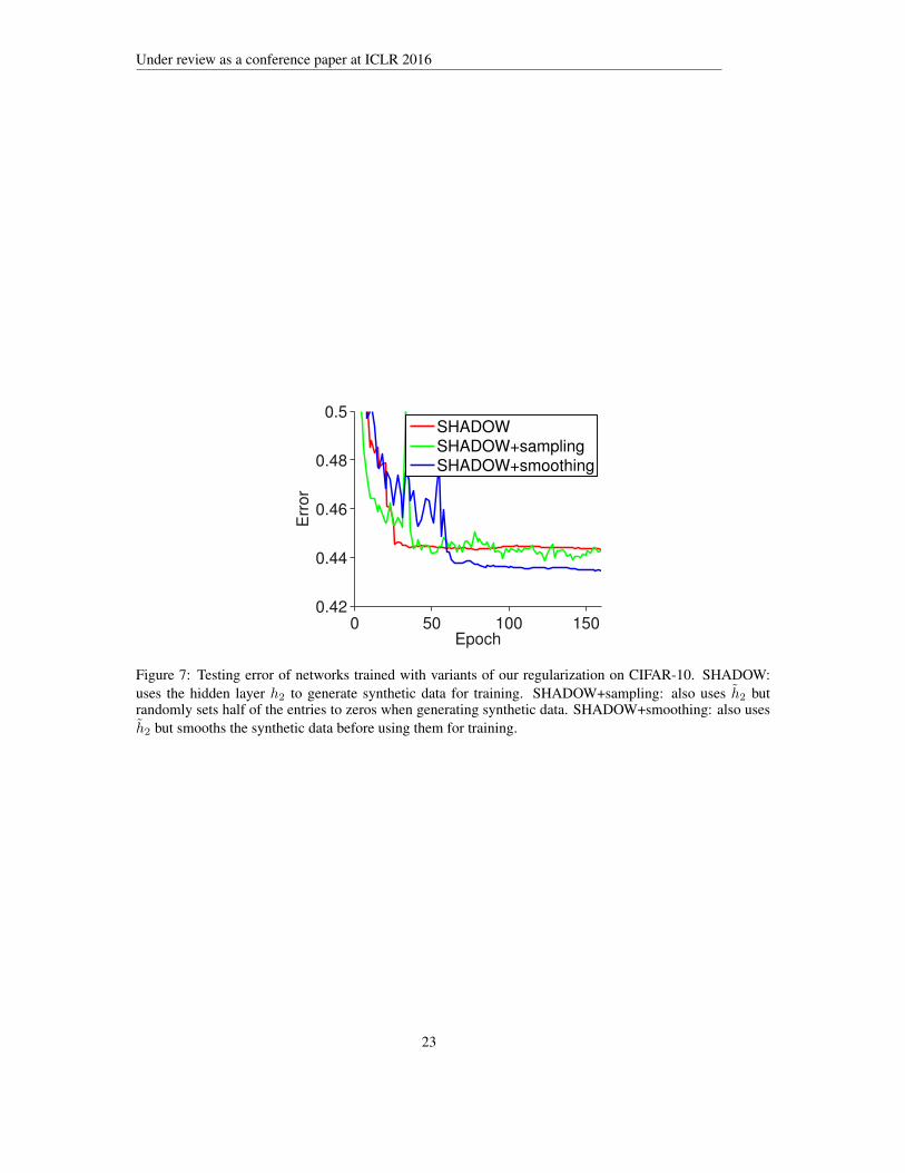
Variants of the SHADOW regularization Instead of using h2 to generate the synthetic data, one can alsouse other layers. Figure 6 compares the results when using h3 and h2. The error when using h3 is similar orbetter than that using h2. This indicates that the images generated from h3 can play a similar role as thosegenerated from h2.

One can also use sampling when generating synthetic images from the hidden layers. More precisely, onecan use

h1 = r(W2h2) ndrop, x′ = r(W1h1) ndrop (27)

where the sampling ratio is 0.5. This adds more noise to the synthetic data and can also act as a regular-ization, since the true distribution should be robust to such noise, as suggested by the success of dropoutregularization. Other prior knowledge about the true distribution can also be incorporated, such as smooth-ness of the images:

h1 = r(W2h2), x′ = r(W1h1), x′′ = Smooth(x′) (28)

21


0 100 200 3000.42

0.44

0.46

0.48

0.5

0.52

Epoch

Err

or

BackpropBackprop+SHADOWError on synthetic

(a) CIFAR10

0 100 200 3000.72

0.73

0.74

0.75

Epoch

(b) CIFAR100

0 100 200 3000.015

0.02

0.025

Epoch

(c) MNIST

Figure 5: Testing error of networks trained with and without our regularization for three datasets. Dropoutwas not used. “error on synthetic” is the testing error on the synthetic data generated from the test set.

0 100 200 3000.4

0.45

0.5

0.55

Epoch

Err

or

BackpropSHADOW(h2)SHADOW(h3)

(a) without dropout

0 100 200 3000.4

0.42

0.44

0.46

0.48

0.5

Epoch

Err

or

DropoutSHADOW(h2) + dropoutSHADOW(h3) + dropout

(b) with dropout

Figure 6: Testing error of networks trained with our regularization on CIFAR-10 using the hidden layer h2or h3 to generate synthetic data.

where Smooth operator sets each pixel of x′′ to be the average of the pixels in its 3× 3 neighborhood. Theperformances of these variants are shown in Figure 7. With sampling, there is larger variance but the erroris similar to that without sampling, in accord with our theory. With smoothing, the error has larger varianceat the beginning but the final error is lower than that without smoothing.

22


0 50 100 1500.42

0.44

0.46

0.48

0.5

Epoch

Err

or

SHADOWSHADOW+samplingSHADOW+smoothing

Figure 7: Testing error of networks trained with variants of our regularization on CIFAR-10. SHADOW:uses the hidden layer h2 to generate synthetic data for training. SHADOW+sampling: also uses h2 butrandomly sets half of the entries to zeros when generating synthetic data. SHADOW+smoothing: also usesh2 but smooths the synthetic data before using them for training.

23

W : A SIMPLE THEORY WITH IMPLICATIONS FOR TRAINING · weight tying idea for denoising...

Documents

Transcript of W : A SIMPLE THEORY WITH IMPLICATIONS FOR TRAINING · weight tying idea for denoising...