Vulnerability Assessment of Low-lying Coastal Areas and … · Page 1 Vulnerability Assessment of...
90
Page 1 Vulnerability Assessment of Low-lying Coastal Areas and Small Islands to Climate Change and Sea Level Rise PHASE 2: CASE STUDY ST. LUCIA Report & SIMLUCIA User Manual Report to UNEP CAR/RCU United Nations Environment Programme Caribbean Regional Co-ordinating Unit, Kingston, Jamaica Guy Engelen, Inge Uljee and Roger White Modelling and Simulation Research Group Research Institute for Knowledge Systems bv P.O. Box 463, Tongersestraat 6 6200 AL Maastricht, The Netherlands Draft Version - October 1997
Transcript of Vulnerability Assessment of Low-lying Coastal Areas and … · Page 1 Vulnerability Assessment of...

Page 1
Vulnerability Assessmentof
Low-lying Coastal Areasand Small Islands
toClimate Change and Sea Level Rise
PHASE 2: CASE STUDY ST. LUCIA
Report & SIMLUCIA User Manual
Report to UNEP CAR/RCUUnited Nations Environment Programme
Caribbean Regional Co-ordinating Unit, Kingston, Jamaica
Guy Engelen, Inge Uljee and Roger White
Modelling and Simulation Research GroupResearch Institute for Knowledge Systems bv
P.O. Box 463, Tongersestraat 66200 AL Maastricht, The Netherlands
Draft Version - October 1997

Page 2
Acknowledgement
We would like to express our gratitude to:• Ms. Beverly Miller and Mr. Vincente Santiago from the UNEP/CAR/RCU office in
Kingston, Jamaica. For their support, not in the least their financial support.
We thank all the St. Lucians that we spoke during our visits, and that helped to gather thenecessary information. In particular:• Mr. Springer, Ms. Louis, Mr. Fevrier, Ms. Charles, Ms. Philbert-Jules, Mr. Jn
Baptiste, Mr. Nickson and Ms. Henry form the Ministry of Planning, Developmentand Environment;
• Ms. Paul, Ms. St. Ville, Mr. Nichols and Ms. Compton from the Ministry ofAgriculture, Lands, Fisheries & Forestry;
• Mr. St. Catherine, Ms. Jean Baptiste, and Mr. Charlemagne from the StatisticsDepartment;
• Ms. Charles from the Ministry of Tourism and Mr. Lewis from the St. Lucia TouristBoard;
• Ms. Chase and Ms. Isaac from the OECS-Natural Resources Management Unit;• Mr. Renard and Mr. Smith from the Caribbean Natural Resources Institute.We hope that SIMLUCIA will become a useful tool to them.
Thanks also to Anthony Filpott and Prof. Alvin Simms from the GIS-lab at MemorialUniversity, St. John’s, Nfld, Canada for their assistance in digitising the maps.
Last but not least we would like to thank: Prof. George Maul, Florida Institute ofTechnology, Melbourne, Fl., USA; Ir. Luitzen Bijlsma and Ir. Leo de Vrees,Rijksinstituut voor Kust en Zee, Rijkswaterstaat, The Netherlands; and Prof. PaulDrazan, Director (retired) of RIKS for encouraging this work with their enthusiasm andsupport.
Guy Engelen, Inge Uljee and Roger WhiteMaastricht, October 1997

Page 3
Important Notice
Please take notice of the following remarks when installing SIMLUCIA.
1. SIMLUCIA has been developed for United Nations Environment Programme,Caribbean Regional Co-ordinating Unit, Kingston Jamaica (UNEP CAR/RCU) aspart of the MOU between UNEP and CIMAS, Miami, Fl, US. SIMLUCIA has beendeveloped by RIKS bv, P.O. Box 463, 6200 AL Maastricht, The Netherlands. Part ofthe modelling work has been carried out by Prof. Roger White, GeographyDepartment, Memorial University, St. John’s, Nfld, A1C 5S7 Canada.
2. If you have on your machine other RIKS applications, such as: GEONAMICA®, the
ISLAND Demo, the CELLCITY Demo, RAMCO, LOKMod, WadBOS, or earlierversions of SIMLUCIA, then put the SIMLUCIA files in a dedicated directory differentfrom the one(s) that contain(s) any of the other applications. Do not interchange filesbetween the different applications as files may have the same names but differentcontents.
3. RIKS is constantly trying to improve its applications. It is our policy to send you the
most recent version of the programs and manuals available. However, as a result, youmay receive an application that is slightly different from the one described in themanual. Do not hesitate to contact us if this would cause you any problems.
4. The RIKS Demos are curtailed versions of more elaborate software products. Each of
the Demos is conceived to allow you to get a good understanding of the full softwareproduct. If you are interested in a demonstration of the full version, you are welcometo contact us.
5. Neither software development with the tools provided in the SIMLUCIA package nor
the application of the SIMLUCIA package to a case study is permitted.Software or application development and further usage or marketing of the SIMLUCIApackage will only be accepted following the purchase of a full version of the package.
Enjoy our Demos and please return your comments to us.
Inge Uljee, Guy Engelen, Roger WhiteRIKSP.O. Box 4636200 AL MaastrichtThe NetherlandsTel. 31-43-388.33.32Fax. 31-43-325.31.55e-mail:[email protected]

Page 4
Table of Contents
1. Introduction _____________________________________________________________ 7
1.1. Summary of the work carried out in Phase 1 ____________________________________ 7
1.2. Phase 2: SIMLUCIA_________________________________________________________ 10
2. Macro-Level Dynamics ___________________________________________________ 11
2.1. The Natural sub-system_____________________________________________________ 112.1.1 Climate ________________________________________________________________________112.1.2 Beach loss ______________________________________________________________________13
2.2. The Social sub-system ______________________________________________________ 152.2.1 Population growth ________________________________________________________________152.2.2 Population ______________________________________________________________________172.2.3 Wealth _________________________________________________________________________17
2.3. The Economic sub-system ___________________________________________________ 182.3.1 External demand _________________________________________________________________192.3.2 Domestic demand ________________________________________________________________192.3.3 Jobs ___________________________________________________________________________20
2.4. Land density calculation ____________________________________________________ 202.4.1 Socio-economic land demand _______________________________________________________202.4.2 Land use _______________________________________________________________________21
2.5. SIMLUCIA: an integrated model ______________________________________________ 22
3. Micro-Level Dynamics ____________________________________________________ 23
3.1. Cellular Automata models___________________________________________________ 23
3.2. A Cellular Automata model for St. Lucia ______________________________________ 24
3.3. GIS information in SIMLUCIA________________________________________________ 283.3.1 The Suitability Calculation _________________________________________________________283.3.2 The Accessibility Calculation _______________________________________________________30
4. Installing SIMLUCIA ______________________________________________________ 31
4.1. What is included in the SIMLUCIA package ? ___________________________________ 31
4.2. Installing SIMLUCIA ________________________________________________________ 31
4.3. Hard- and Software Requirements ___________________________________________ 31
4.4. Installation procedure for Windows 95 ________________________________________ 31
4.5 Installation procedure for Windows 3.x ________________________________________ 324.5.1 Running SIMLUCIA under Microsoft Windows 3.1x ______________________________________334.5.2 How to get Microsoft Win32s version 1.3______________________________________________334.5.3 Installing SIMLUCIA under Microsoft Windows 3.1x _____________________________________33
4.6. Starting SIMLUCIA _________________________________________________________ 34
4.7. Screen Layout _____________________________________________________________ 344.7.1 The Control Menu Box ____________________________________________________________35

Page 5
4.7.2 The Caption Bar _________________________________________________________________354.7.3 The Menu Bar ___________________________________________________________________354.7.4 The Tool bar ____________________________________________________________________364.7.5 The Status bar ___________________________________________________________________36
4.8. Getting Help ______________________________________________________________ 37
4.9. Exiting SIMLUCIA__________________________________________________________ 37
4.10. If you experience problems _________________________________________________ 37
5. Running SIMLUCIA Simulations ____________________________________________ 38
5.1. Running a simulation_______________________________________________________ 385.1.1 The Micro-scale dynamics Window __________________________________________________395.1.2 The Macro-scale dynamics Window __________________________________________________41
5.2. Starting the simulation. _____________________________________________________ 44
5.3. Viewing model output ______________________________________________________ 45
5.4. Saving simulation results____________________________________________________ 46
5.5. Printing simulation results __________________________________________________ 47
6. The SIMLUCIA Menu System _______________________________________________ 49
6.1. The File Menu_____________________________________________________________ 496.1.1 New simulation Command _________________________________________________________496.1.2 Open simulation Command _________________________________________________________496.1.3 Save simulation Command _________________________________________________________506.1.4 Import file... Command ____________________________________________________________506.1.5 Export file... Command ____________________________________________________________506.1.6 Page Setup Command _____________________________________________________________506.1.7 Print Command __________________________________________________________________506.1.8 Print Preview Command ___________________________________________________________506.1.9 Print Setup Command _____________________________________________________________506.1.10 List of Recent File (1, 2, 3, 4) ______________________________________________________516.1.11 Exit Command__________________________________________________________________51
6.2. Edit Menu ________________________________________________________________ 526.2.1 Pen Command ___________________________________________________________________526.2.2 Fill Command ___________________________________________________________________526.2.3 Precision Command_______________________________________________________________52
6.3. View Menu _______________________________________________________________ 536.3.1 Go to... Command ________________________________________________________________536.3.2 Zoom in Command _______________________________________________________________536.3.3 Zoom out Command ______________________________________________________________536.3.4 Show regions Command ___________________________________________________________536.3.5 Show network Command___________________________________________________________536.3.6 Show elevation Command __________________________________________________________536.3.7 3D settings Command _____________________________________________________________54
6.4. Maps Menu _______________________________________________________________ 556.4.1 Land use Command _______________________________________________________________556.4.2 Elevation Command ______________________________________________________________556.4.3 Network Command _______________________________________________________________556.4.4 Suitability Command ______________________________________________________________566.4.5 Regions Command________________________________________________________________566.4.6 Potential Command _______________________________________________________________57
6.5. Rules Menu _______________________________________________________________ 586.5.1 (land use) Command ______________________________________________________________586.5.2 Overview Command ______________________________________________________________58

Page 6
6.6. Simulation Menu __________________________________________________________ 596.6.1 Init Command ___________________________________________________________________596.6.2 Step Command __________________________________________________________________596.6.3 Run Command___________________________________________________________________596.6.4 Stop Command __________________________________________________________________596.6.5 Reset Command__________________________________________________________________596.6.6 Pauses ... Command_______________________________________________________________606.6.7 Random ... Command _____________________________________________________________60
6.7. Options Menu _____________________________________________________________ 616.7.1 Grid ... Command ________________________________________________________________616.7.2 Font ... Command ________________________________________________________________616.7.3 Link to Excel … Command _________________________________________________________616.7.4 Log ... Command _________________________________________________________________616.7.5 Tool bar Command _______________________________________________________________616.7.6 Status bar Command ______________________________________________________________62
6.8. Window Menu ____________________________________________________________ 636.8.1 Cascade Command _______________________________________________________________636.8.2 Tile Horizontal command __________________________________________________________636.8.3 Tile Vertical Command ____________________________________________________________636.8.4 Arrange Icons Command___________________________________________________________636.8.5 Close windows Command __________________________________________________________636.8.6 List of Windows (1, 2, 3, 4, ...) ______________________________________________________63
6.9. Help Menu________________________________________________________________ 646.9.1 Index Command _________________________________________________________________646.9.2 Using Help Command _____________________________________________________________646.9.3 About ... Command _______________________________________________________________64
7 ANALYSE ________________________________________________________________ 65
7.1 Basic concepts and features __________________________________________________ 65
8. Policy exercises with SIMLUCIA _____________________________________________ 68
8.1 Introduction _______________________________________________________________ 68
8.2 Exercise a: Working with scenarios ___________________________________________ 69
8.3 Exercise b: Working with ANALYSE and MS Excel _______________________________ 72
8.4 Exercise c: Working with policy interventions___________________________________ 74
9 References ______________________________________________________________ 78
ANNEX A: GEONAMICA Simulation Environment ____________________________ 79
ANNEX B: Estimation of the Input-Output Table ________________________________ 82
I. Introduction ________________________________________________________________ 82
II. Derivation of the Output (or Demand) Side of the Table___________________________ 83
III. Derivation of the Input (or Supply) Side of the Table ____________________________ 84
IV. Derivation of the Inter-Industry Portion of the Table ____________________________ 86
V. Note on Employment and Productivity _________________________________________ 86
ANNEX C: Factors and Weights______________________________________________ 88
ANNEX D: Pointer Shapes __________________________________________________ 90

Page 7
1. Introduction
This report covers the activities of RIKS in Phase 2 of the UNEP project ’VulnerabilityAssessment of Low-lying Coastal Areas and Small Islands to Climate Change and SeaLevel Rise’.
The long term objectives of this project are to develop a methodology and operationalprocedure applicable on the level of the individual coastal country or island (1) todescribe and analyse the impacts of climate change on their territory, their ecosystems,their social systems and their economic activities, and (2) to provide instruments or toolsto design, explore and evaluate policy measures and policy interventions to prevent oralleviate undesirable impacts.
Phase 1 of the project proposed a generic modelling methodology and decision supportsystem judged to be capable of fulfilling, at least partially, both requirements posed inthe objectives. More than being a theoretical exercise, the project produced ademonstrator version of the decision support system developed.
The specific objectives of Phase 2 of the project are to apply the modelling methodologyand decision support system to St. Lucia, West Indies and to adapt them to the extentrequired.
1.1. Summary of the work carried out in Phase 1
Climate change in the Wider Caribbean Region is expected to have an important impacton the physical, environmental, social and economic systems (Maul, 1993). Socio-economic systems in the region are already stressed considerably due to demographic,economic and environmental factors, and climate change will exacerbate this situation.Hence, formal instruments to study the effects of climate change on socio-economicsystems require realistic representations of their actual state and of the mechanisms thatwill cause them to change in the future. Their temporal and spatial dynamics should bewell represented, because climate change is affecting socio-economic systems throughmechanisms at very different geographical scales: at the Macro-scale causing changes inthe exchanges with the world system through changed demands, exports, imports andmigrations; and at the Micro-scale causing the relocation and possible disappearance ofactivities.
With a view to realistically describe the effects of climate change on socio-economicsystems we developed an explicitly dynamic (temporal) and spatial modelling frameworkoperating at two geographical levels: the Macro-level describes the macro-economic andlong-range spatial interactions, and the Micro-level describes the short-range interactionsand location choices. This modelling framework has been applied to and tested on atheoretical, prototypical, island (named ISLAND) with characteristics typical of existingsmall Caribbean islands. At the Macro-level, ISLAND is modelled as a single region --asone point in space interacting with the external world. Hence, a single set of linkeddynamic equations generates the evolution in time of the integrated socio-economic and

Page 8
environmental systems. The growthcoefficients thus calculated are fedinto a cellular model, operating on theMicro-level, which allocates the socio-economic growth to island cells of 500by 500 meter. This allocationmechanism is based on Micro-levelspatial interactions specified incellular automata rules and based onphysical suitability measures retrievedfrom a GIS. The cellular model willreturn the results of the allocation tothe Macro-level, thus guaranteeing thefull coupling of the macro and microscales.
At the Macro-level essentially threecoupled sub-systems are modelled: thenatural, social, and economic sub-systems. The proposed modellingframework allows for different typesof mathematical representations ofeach of these sub-systems, thusallowing for a more or less detaileddescription of certain aspects of thesub-systems. In the first phase of theproject we have selected modelrepresentations that fit the applicationof the modelling framework to thehypothetical small island. It reflectsthe archetype nature of the work andleaves room for a number ofimprovements. The economic sub-system is modelled by means of ahighly aggregated input-output model,coupled with the demographic model(through a wealth indicator andhousehold demands), with the naturalsystem (climate changes influenceexternal demand) and with the Micro-level via a land density expression(activities require space).
The economy is aggregated into five sectors. In the social sub-system the ISLANDdemography is modelled as a single population group growing as the result of births,deaths, and migration. The birth rate is specified to follow a long term trend, whilemortality and migration rates depend on both forecasted long term structural trends, andon the well-being of the island population as indicated by the employment participationrate. The natural sub-system consists of a set of linked relations representing theexpected change in time of sea level and temperature, and their effects on the loss ofland, on precipitation, storm frequency, and external demands for services and products.Later, the natural sub-system could be further developed to include a description of thegrowth of natural systems such as coral reefs, mangroves, and beaches. The model
Figure 1: A modelling framework consisting of coupledmodels at the Macro-level and the Micro-level.

Page 9
provides the slots to plug in such modules, but further research will be required todevelop and implement them.
At the Macro-level, the model calculates the changes in employment per sector and thegrowth of the population. New jobs and new people will require space to support theirresidential and economic activities. In the model the translation of economic andresidential activity into space is performed by means of the land density expression. Theland density is a function of the total amount of land available, the suitability of that landfor the activities carried out, and the land (and its suitability) already occupied.Generally speaking, land density will increase if land is getting scarce. But it willdecrease if the land occupied is getting marginal for use by the specific activity. Thetotal amount of land required by each activity is used as an input to the Micro-level partof the model.
More than in the Macro-scale representation, the principle mechanism underlying theMicro-scale dynamics is the fact that socio-economic activities will interact with oneanother in geographical space. It is a well documented phenomenon in regionaleconomics and is common to concepts such as economies of scale, agglomerationadvantages, distance decay, push and pull forces. It translates the fact that activity Xdoes not flourish in the neighbourhood of activity or feature Y, while Z does very wellnear Y. These push and pull forces are expressed in the cellular model by means ofattraction-versus-distance functions for each pair of activities or land-uses modelled. Butthis functional appropriateness of a cell is not by itself sufficient to decide the likelihoodthat the cell will be occupied by one or the other activity. Its intrinsic physical suitabilitywill also have to be right. The physical suitability of a cell is an aggregate measurecalculated from a number of physical indicators (and may include infrastructural andlegislative factors as well). These calculations are standard operations in state of the art(commercially available) GIS packages. Hence the coupling of the modelling frameworkwith a GIS package is envisaged.
It is by means of Cellular Automata rules that we calculate the changing land-use on theMicro-level. Rules are applied hierarchically. The highest priority is given to userinterventions, including the forced location of an activity in a specific area, or thedevelopment of an area for a specific use, etc. The next highest priority involves theelevation of a cell relative to the sea level. These rules decide on the total amount ofland available for the different activities and on the physical suitability of such land. Thelowest priority is for rules that calculate the aptness of a cell to receive a specific activity.This aptness is a function of the physical suitability of the cell and the activities alreadypresent in its neighbourhood.
The model thus defined is the core element of the DSS (Decision Support System) thatwe began to implement. In the DSS the model is complemented with user-friendly andinteractive software tools which make it very easy to use and which facilitate thedecision making process.
Phase 1 of the project involved the application and testing of the modelling frameworkon the basis of a theoretical application only. It suggested that the framework would beapplied to a real case and that a thorough validation and calibration would be carriedout.
The results of phase 1 have been documented in Engelen et al., 1993a, Engelen et al.,1993b and Engelen et al., 1995. The demonstrator developed in phase 1, called ISLANDDemo, can be obtained from RIKS, or, for those having access to Internet, can bedownloaded from the RIKS’ homepage: http://saturn.matriks.unimaas.nl

Page 10
1.2. Phase 2: SIMLUCIA
The remainder of this report deals with the second phase of the project ’VulnerabilityAssessment of Low-lying Coastal Areas and Small Islands to Climate Change and SeaLevel Rise’, which mainly involves the application of the modelling and decisionframework to the case of St. Lucia. The resulting model and software system has beengiven the name SIMLUCIA. In Chapter 2 the development and implementation of themodels at the Macro-level is discussed, while Chapter 3 gives more details on the Micro-level models. Chapters 4, 5, 6 and 7 cover the contents of the user manual for SIMLUCIA,and finally Chapter 8 demonstrates the use of SIMLUCIA in a policy context.

Page 11
2. Macro-Level Dynamics
The Macro-level model (Figure 2) essentially models three coupled sub-systems eachrepresented by sets of linked variables: the natural sub-system, the social sub-system andthe economic sub-system.
Figure 2: Schematic representation of the Macro-level of the model showing the loops linking thenatural, the social and economic sub-systems.
2.1. The Natural sub-system
The natural sub-system consists of a set of linked relations expressing the change in timeof temperature and sea level, and the effects of these on precipitation, storm frequencyand external demands for services and products from St. Lucia. The hypothesis is madethat climate change only affects the external demand for products produced in St. Luciathus expressing changing world markets as well as the manner in which the island’sproducts and services is perceived in the external world (e.g. by possible clients, touristsor investors). In this version of the model these relations are entered directly by the userand either represent state of the art knowledge, outputs of other models including globalcirculation models, climatic change models and greenhouse gas models, or the scenariosor sets of hypotheses with which the model is run.
2.1.1 Climate
definition:The expressions used in the Climate MBB1 assume a simple and direct relation betweentwo variables. However, the definition of changes in precipitation and storm frequency
1 The acronym MBB stands for Model Buiding Block and refers to a sub-model. (See also Annex A.)

Page 12
for example, as a function of temperature only is a strong simplification of reality. Inmore elaborate versions of the model, such relations could be replaced by dedicated sub-models capable of describing them at a deeper, causal level. Similarly, the model of theNatural sub-system could include a description of the growth of natural systems such ascoral reefs, mangroves, sea grasses, riverine systems and beaches.
mathematical formulation:( )T f tt T=( )L f tt L=
( )P f Tt P t=
( )F f Tt F t=
( ) ( ) ( )[ ]E e f T f P f Fi t i t t t t, ,= + + +1 )
( )( ) [ ]E e
N
NT P Ftourism t tourism t
beach t
beach t
t t t, ,
,
,
exp
exp=
− −
− −+ + +
=
1
11
0
β α
β αwith:t timef() function ofEi t, Vector of sectoral external demand; [million EC$]
Tt Temperature change; [Celsius]
Lt Sea level change; [feet]
Pt Precipitation change; []
Ft Storm frequency change; []
Nbeach t, Number of beach cells; [cells]
ei t, Vector of projected sectoral external demand ceteris paribus; [million EC$]
α Resilience of tourism industry; []β Relative importance of beach tourism in total tourism industry; []
calibration information:
Figure 3: Most relations of the natural sub-system are defined as tables. The figure shows on theleft the relation between time and temperature change and on the right the effect of temperaturechange on storm frequency.

Page 13
The relations used in SIMLUCIA are pure hypothesis expressing how the economy couldbe influenced by climate change. Some general trends of these expressions have beendiscussed with the scientists and members of the UNEP/IOC Task Team on theImplications of Climatic Change in the Wider Caribbean Region. These trends are goodestimates for the St. Lucian situation, without them being scientifically proven. Theygenerally reflect the dependency of the agriculture and the tourism sector on the actualclimatic conditions. The user is free to correct or replace the hypotheses with betterinformation if it is available, or he can experiment with other hypotheses in order to findout how different climate related scenarios would (possibly) affect the St. Lucianeconomy.
Part of the natural sub-system concerns a measure of the physical and environmentalsuitability (or aptness) of each Micro-level region (called cells in the cellular model) ofSt. Lucia for receiving one of the activities modelled. This information is available fromthe GIS (Geographical Information system) and its digitised maps. Changing sea levelwill cause the loss (or gain) of low-lying coastal areas and will cause the total availablearea to shrink (or to grow). This mechanism of losing or gaining land is modelled in theMicro-level cellular automata model and is described in more detail in Chapter 3. Losingor gaining land will affect the total suitability of the land area and will put more or lessstress on the land used by the different economic activities. This effect is expressed bymeans of the concept of land density and explained under that heading in this chapter.Hence, broadly speaking, the natural sub-system will translate the changes in temperatureand sea level into changes in the total land area, changes in the suitability of that landarea and in changed external demands for goods produced on the island.
2.1.2 Beach loss
definition:Changing sea level will cause the loss (or gain) of beach area. This sub-model expressesthe fact that beach area is a very important asset for the tourism industry. Hence, that theloss of beach might damage the industry a great deal. This is certainly the case for St.Lucia where tourism is mainly beach related and where the total beach area is limited. Inthe event that due to climate change beaches would disappear rapidly, St Lucia willquickly lose its image in the outside world and gradually the demand for tourism wouldfall.
mathematical formulation:
( )( ) [ ]E e
N
NT P Ftourism t tourism t
beach t
beach t
t t t, ,
,
,
exp
exp=
− −
− −+ + +
=
1
11
0
β α
β αwith:Etourism t, External demand for tourism; [million EC$]
Tt Temperature change; [C]
Lt Sea level change; [feet]
Pt Precipitation change; []
Ft Storm frequency change; []
Nbeach t, Number of beach cells; [cells]
etourism t, Projected external demand ceteris paribus for tourism; [million EC$]
α Resilience of tourism industry; []β Relative importance of beach tourism in total tourism industry; [%]

Page 14
calibration information:
( )( )y
N
N
beach t
beach t
=− −
− − =
1
1 0
β α
β α
exp
exp
,
,
The two parameters in the expression take into consideration the effect of both (1) therelative importance of beach tourism in the total tourism industry (parameter β ) and (2)the sensitivity of the industry to the phenomenon of a disappearing beach (parameter α ).In the graph underneath, three cases, representing different combinations of α and β ,are shown. Generally speaking, an old, well established or rich tourism industry will dowhatever is in its power to prevent itself from vanishing (Case 2), while a young or poorindustry does not have the possibilities to do so (Case 1). Case 3 shows the trend of therelation with the parameter values used for St. Lucia. Note however that the initial (att=0) number of beach cells in St. Lucia is only 34.
0
0.2
0.4
0.6
0.8
1
1.2
1.4
1.6
0 50 100 150 200 250 300 350
Beach cells at time t
Dem
and
for
tour
ism
(y)
Case 1 Case 2 Case 3
Case 1 Case 2 Case 3α 0.01 0.05 0.01β 0.9 0.6 0.6
Beach Cells at t=0 100 100 100
default values:For St. Lucia, the values for the parameters are as follows:α = .05; β = .90;these values reflect the fact that the tourism industry depends largely (90%) on thepresence of beaches, but, that it has a high level of resilience to counteract the effects ofbeach degradation. In other words, it can afford to an extent beach nourishment or beachprotection programmes.

Page 15
2.2. The Social sub-system
The social sub-system describes the demography of St. Lucia and the social well-being ofits population. The demography is modelled as a single population group growingexponentially as the result of births, deaths and migrations. The social well-being isexpressed as the employment participation rate, meaning the proportion of people havinga paid job.
2.2.1 Population growth
definition:This sub-model calculates the population growth in St. Lucia. The population is growingexponentially as the result of births, deaths and migrations. The mortality rate andmigration rate both have a structural component and an economic component. Thestructural component expresses the long term structural change which is valid for St.Lucia or the larger region of which it is part. It represents long term trends set in motionas a result of family planning policies, education, health care programs, etc. It reflectsfor instance improving (or worsening) living conditions that gradually penetrate the area(and affect the mortality rate), traditional migration trends and general evolution of thewell-being of the neighbouring countries (which affect the migration flows). Grafted onthis is a socio-economic component expressing improved living conditions and economicprosperity in St. Lucia itself.
mathematical formulation:( )bb f tt b=
( )( )( )[ ]
dd f tr u u
t d
t t=
+ − − =1 3
2
0exp
( )[ ][ ]mm r
r u u
rt
t t= +
− −−
−=
41 5
1 51
0exp
( )∆p p bb dd mmt t t t t= × − −p p pt t t+ = +1 ∆
with:pt Total population; [persons]bbt Birth rate; [1/1000]ddt Mortality rate; [1/1000]mmt Migration rate; [1/1000]Xi,t Vector of sectoral employment; [persons]ut Wealth or employment participation rate; []
( )f tb Structural reproduction rate; [1/1000]
( )f td Structural mortality rate; [1/1000]r3 Variable mortality rate; [1/1000]r4 Structural migration rate; [1/1000]r5 Variable migration rate; [1/1000]
calibration information:
expression: ( )( )( )[ ]
dd f tr u u
t d
t t=
+ − − =1 3
2
0exp

Page 16
The total mortality rate is the sum of a structural component (parameter ( )f td ) and acomponent reflecting the wealth of the population (parameter r3). The graph showsdifferent curves for different hypothesis concerning the latter.
0
5
10
15
20
25
-1.5 -1 -0.5 0 0.5 1 1.5
Change in wealth
Tot
al M
orta
lity
Rat
e
Case 1 Case 2 Case 3
Case 1 Case 2 Case 3
( )f td7 7 7
r3 0.5 1 1.5
expression: ( )[ ]
[ ]mm rr u u
rt
t t= +
− −−
−=
41 5
1 51
0exp
-12
-8
-4
0
4
8
12
-1.5 -1 -0.5 0 0.5 1 1.5
Change in wealth
Tot
al M
igra
tion
Rat
e
Case 1 Case 2 Case 3

Page 17
Case 1 Case 2 Case 3r4 -5 1 5r5 0.6 0.6 0.9
Total migration rate is the sum of a structural component (parameter r4) and acomponent reflecting the wealth of the population (parameter r5). The figure shows thecurves reflecting different cases.
default values:The values used for St. Lucia have been calculated from the Annual Statistics Digest1991 and personal communications from the Government Statistics Department.
2.2.2 Population
definition:In SIMLUCIA, the assumption is made that there will be a growing concentration of thepopulation in urban areas. There is however not an expression that will calculate thedegree of urbanization on the basis of demographic or economic pressure. Rather, in thisversion of the model, the proportion of the population living in urban areas is read in as ascenario defined by the user.
mathematical formulation:( )
( )
up p f t
rp p f t
t t u
t t u
=
= −
1
with:upt Urban population; [persons]
rpt Rural population; [persons]
pt Total population; [persons]
( )f tu Proportion of the population living in urban areas; [%]
default values:In the model the assumption is made that a growing percentage of the population of St.Lucia will be living in urban areas in the next 40 years. In 1990, the urban populationwas estimated (from the population statistics) to be 36.1 %, and the hypothesis is madethat this proportion will increase to a value of 54.01 % in 2030.
2.2.3 Wealth
definition:The social well-being is expressed as the employment participation rate, meaning theproportion of people having a paid job.
mathematical formulation:
u
X
pt
i ti
t
=∑ ,
with:

Page 18
ut Wealth or employment participation rate; [%]
pt Total population; [persons]
X i t, Vector of sectoral employment; [persons]
2.3. The Economic sub-system
The economy of St. Lucia is modelled by means of a highly aggregated input-outputmodel which is coupled to the demographic sub-model. The input-output modeldescribes the economy of the island as a set of linear equations. We use the input-outputmodel in a quasi dynamic manner by evaluating it at each iteration: at each time step andfor each economic sector new demand, generated externally or internally by thepopulation and the economic sectors, is translated into new job opportunities andchanged needs for imports. We have chosen to model the economic sub-system bymeans of an input-output model because of its representation of the interdependenciesbetween economic sectors, and the way it integrates imports and final demands. Hence itdescribes well the economic multiplier effects and will show how changes in oneeconomic sector will propagate throughout the whole economy. The input-output modelused is of a type in which the technical coefficients do not change over time (nondynamic). This means that it is assumed that the economic mix does not changesignificantly in the period for which the model is applied. This is a very weakhypothesis, certainly for long term modelling and for economies which are highlytechnical in nature and where technological innovations and substitutions are veryfrequent (which has not been the case for St. Lucia in the past). In principle the modelwill have to be re-calibrated (that is the technical coefficients need to be recalculated)every time substitution has taken place. Else, the numbers generated have to beinterpreted bearing in mind the fact that the model assumes constant input and outputcharacteristics for each type of activity. Despite the many deficiencies of this type ofmodel, it is one of the most widespread techniques to describe an economy and manynational or regional planning and statistics agencies will use it (Richardson, 1978).Hence very often data for the model will be readily available.
mathematical formulation:∆ ∆ ∆Y Dom Ei t i t i t, , ,= +Y Y Yi t i t i t, , ,= +−1 ∆
∆ ∆ ∆S A S Yi t i jj
j t i t, , , ,= +∑ −1
S S Si t i t i t, , ,= +−1 ∆∆ ∆M I Si t i i t, ,= ×M M Mi t i t i t, , ,= +−1 ∆
∆∆
XS
Bi t
i t
i,
,=
with:Si t, Vector of total sectoral outputs; [million EC$]
Yi t, Vector of final demands (domestic + external demand); [million EC$]
X i t, Vector of sectoral employment; [million EC$]
Mi t, Vector of sectoral imports; [million EC$]

Page 19
Domi t, Vector of sectoral domestic demands; [million EC$]
Ei t, Vector of sectoral external demands; [million EC$]
Ai j, Matrix of technical coefficients for endogenous sectors; []
Ii Vector of import coefficients; [million EC$]
calibration information:Since no input-output model for the base year 1990 was available in St. Lucia, we haveestimated a simplified 5-sector input output table on the basis of the following:• Ministry of Agriculture, Lands, Fisheries and Forestry: Annual Agricultural Statistics
Digest 1992• Government Statistics Department: National Accounts 1977 to 1992• Government Statistics Department: Annual Statistical Digest 1991• St. Lucia Tourist Board: Selected Tourism Statistics• St. Lucia Tourist Board: St. Lucia Stay Over Visitors Survey – Summer 1995A detailed description of the estimation procedure can be found in Annex B of thisreport.
2.3.1 External demand
definition:The external demand per sector is defined as an externally provided time series. Thetime series per sector are to be derived from the long term economic forecasts andcalculated under conditions of no climate change. If such forecasts are not available, thetime series reflect best estimates, hypotheses or scenarios entered by the user.
mathematical formulation:( )e f ti t e, =
with:ei t, Vector of projected external demands ceteris paribus; [million EC$]
calibration information:Detailed long term economic forecasts per sector were not available in St. Lucia. Thetime series entered for the different economic sectors are pure hypotheses. They reflect atransition from an agriculture and tourism based economy towards a more industry andservices based economy.
2.3.2 Domestic demand
definition:This sub-model calculates the domestic demand as the product of the consumption perhead of goods from each economic sector and the total population. The consumption perhead varies as a function of the level of wealth, thus expressing the fact that people spenda larger proportion of their total budget on elementary goods (food) when the level ofwealth decreases.
mathematical formulation:
( )( )∆ ∆Dom C n u u pi t i i t t t, exp= × × − ×=0
with:
Page 20
Domi t, Vector of sectoral domestic demands; [million EC$]
ut Wealth or employment participation rate; [%]
pt Total population; [persons]
Ci Vector of sectoral domestic demand coefficients; [million EC$]
ni Vector of influences of wealth on domestic consumption; [million EC$]
calibration information:In order to estimate the effect of wealth on the consumption behaviour of people, adetailed survey is required. Such a survey was not available. As a result, no effect ofwealth on the consumption behaviour is assumed ( ni = 0 for all economic sectors)
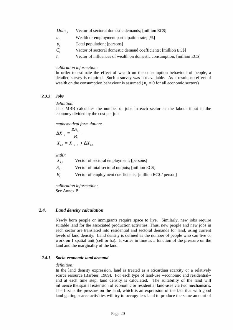
2.3.3 Jobs
definition:This MBB calculates the number of jobs in each sector as the labour input in theeconomy divided by the cost per job.
mathematical formulation:
∆∆
XS
Bi t
i t
i,
,=
X X Xi t i t i t, , ,= +−1 ∆
with):X i t, Vector of sectoral employment; [persons]
Si t, Vector of total sectoral outputs; [million EC$]
Bi Vector of employment coefficients; [million EC$ / person]
calibration information:See Annex B
2.4. Land density calculation
Newly born people or immigrants require space to live. Similarly, new jobs requiresuitable land for the associated production activities. Thus, new people and new jobs ineach sector are translated into residential and sectoral demands for land, using currentlevels of land density. Land density is defined as the number of people who can live orwork on 1 spatial unit (cell or ha). It varies in time as a function of the pressure on theland and the marginality of the land.
2.4.1 Socio-economic land demand
definition:In the land density expression, land is treated as a Ricardian scarcity or a relativelyscarce resource (Barbier, 1989). For each type of land-use --economic and residential--and at each time step, land density is calculated. The suitability of the land willinfluence the spatial extension of economic or residential land-uses via two mechanisms.The first is the pressure on the land, which is an expression of the fact that with goodland getting scarce activities will try to occupy less land to produce the same amount of

Page 21
economic output. Pressure on land is defined as the amount of suitable land occupied bya sector as a proportion of the total suitable land available for that sector. The latter isthe suitable land already taken in by the activity and land in the ‘Natural’ and ‘Forest’state. The second mechanism concerns the marginality of the land, expressing the factthat as good land is getting scarce, activities will have to occupy less adequate --or moremarginal-- locations and hence more land is required to obtain the same amount ofoutput. The marginality of the land is the average suitability of the land occupied by thesector. The combined effect of both mechanisms is reflected in the land densitycalculation.
mathematical formulation:
WX
Ni
i
i,
,
,0
0
0
=
W WSS
TS
TS
SS
SS
N
N
SSi t i
i t
i t
i i t
i t
i
i
i
i
i
, ,
,
,
, ,
,
,
,,
=
0
0 0
00
σ ζ
with:the subscript i includes the sector ‘residential’ otherwise represented as p
Wi t, Vector of land densities; [persons /cell]
SSi t,
Vector of suitabilities summed over the cells occupied by the activity; []
TSi t,
Vector of suitabilities summed over all ,Natural’ and ‘Forest’ cells; []
Ni t,
Vector of total cells required; [cells]
X i ,0 Vector of sectoral employment, including the sector residential; [persons]
σi vector of sectoral sensitivities to land pressure; []
ζ i vector of sectoral sensitivities to land quality (marginality); []
Calibration information:In the model, the initial values for the land density ( 0,iW ) are calculated from the land
use map (to calculate the total amount of land taken in by each activity) and the datafrom the demographic and the economic sub-model. If the user changes the original landuse map, the population or economic data, the model will automatically adjust the initialland densities. The parameters σi and ζ i have been calibrated based on data obtainedfrom (personal communications) the Ministry of Agriculture (minimum and maximumarea of farm and estate land per person employed) and the Ministry of Tourism(minimum and maximum hotel area per person employed).
2.4.2 Land use
definition:The total demand for land is calculated as the total amount of jobs or residents that haveto be allocated at a given density. These demands for land are then passed onto theMicro-level model for allocation on the basis of short range interaction mechanisms andenvironmental factors reflected in the suitability maps.
mathematical formulation:

Page 22
NX
Wi ti t
i t,
,
,
=
tp
ttp W
pN
,, =
with:
Ni t,
Vector of sectoral total cells required; [cells]
tip , Total population; [persons]
X i t, Vector of sectoral employment; [persons]
Wi t, Vector of land densities; [persons/cell]
2.5. SIMLUCIA: an integrated model
Although the sub-systems have been dealt with separately, they are strongly inter-linkedwith one another via the feedback loops that are built into the model. The most essentialof these are shown in Figure 2. This scheme allows to follow through the calculationsthat the model performs at each simulation time step. It also allows to reason in aqualitative manner about direct and indirect impacts of climate change on the island. Asan example of this, one can follow through the following chain of effects: (interpret thesymbol ‘→‘ as ‘this will have an effect on’): imagine a temperature rise of 2°C and sealevel rise of 10 cm by 2025 → the external demand for tourism, namely: a drop innumber of tourists → the total demand for hotel facilities and services → constructionand maintenance of hotels, the creation of new services and the number of jobs (in thetourism and construction sector) → jobs → wealth → mortality and migration rates (e.g.a drop in the number of jobs in the tourist sector leads to higher unemployment rates,which influences people’s decision to migrate out, leading to a decreasing totalpopulation, which in turn decreases the amount of residential land required). Notice alsothe loop indicating the natural loss of available land due to the rising sea level.
Due to the globally non-linear character of the model and the high degree of linkageamong the variables, the set of equations can not be solved analytically; rather theirsimultaneous solution is simulated numerically on the computer as a time trajectory forthe state of the system.
In summary, in the Macro-level model the growth of the population is a result of longterm demographic trends and the economic output. Growth in the different economicsectors is the result of changes in the demands for goods of these sectors. Externaldemand is subject to the effects of climatic change. The density calculation will translatethe growth coefficients of each sector in changing demands for land. The allocation ofactivities to specific locations takes place in the Micro-level of the model. The nextchapter will deal with the modelling technique that performs this allocation on the basisof local interaction mechanisms.

Page 23
3. Micro-Level Dynamics
In St. Lucia, like in most other small islands and coastal nations, activities are stronglyconcentrated in a narrow coastal zone. This results in conflicts of interest andcompetition for space and causes irrecoverable stress on the unique but fragile terrestrialand marine ecosystems of the coastal zone. Hence, it is very important to have a goodunderstanding of the processes that affect the coastal zone directly but also indirectly.More than this, it is essential to know where the coastal zone will be affected, becausesocio-economic pressure is never ‘average’, nor is it ‘constant’ in time or distributed‘evenly’ over the coastal zone. Rather, socio-economic pressure is variable in time andin space as it is the result of the interaction between mobile social and economic agents.Thus, even if we are able to learn from our Macro-level model that a particular economicsector, such as tourism, could be largely affected by changing climatic conditions, thatwould not tell us were on the island such changes would take place, nor what conflicts itwould create with other activities. Clearly, the knowledge as to whether changes willconcentrate in one location or another, or will spread out over large parts of the coastalzone is of great importance in estimating the real effects of the development.
3.1. Cellular Automata models
At the descriptive level, some of this information can be captured in a GeographicalInformation System. Dynamic modelling and prediction, however, requires going farbeyond the capabilities of a GIS. In our modelling framework, advantage is taken to theextent possible of the functionality offered by GIS, such as: data management, datatransformation, data vizualisation, cartographic modelling and spatial analysis. On theinformation rich GIS data-layers dynamic socio-economic and socio-environmentalmodels are built that threat space as consisting of a two-dimensional matrix of smallcells. On this grid we develop a Constrained Cellular Automata model representing theland use dynamics of the island.
Cellular Automata can be thought of as very simple dynamic spatial systems in which thestate of each cell in an array depends on the previous state of the cells within aneighbourhood of the cell, according to a set of state transition rules. Because the systemis discrete and iterative, and involves interactions only within local regions rather thanbetween all pairs of cells, a Cellular Automaton is very efficient computationally. It isthus possible to work with grids containing tens of thousands of cells. The very finespatial resolution that can be attained is an important advantage when modelling land usedynamics, especially for planning applications, since spatial detail represents the actuallocal features that people in a city experience, and that planners must deal with.
A cellular automaton consists of (Langton, 1986):1. an Euclidean space (two-dimensional in our application) divided up into an array of
identical cells;2. each cell is surrounded by a neighbourhood of the same size and geometrical shape,3. each cell is in one of n discrete possible states (land-uses in our application),

Page 24
4. transition rule(s), possibly of a hierarchical nature, describe the new state of a cell asa function of its own state and the state of the cells in its neighbourhood,
5. time progresses uniformly, and at each discrete time step, all cells simultaneouslychange state as defined in the transition rule(s).
In purely practical terms the cellular model will calculate how land use is changing fromyear to year. To that end it will perform a calculation for each cell of the grid. Thiscalculation will be done within the neighbourhood of the cell, which consists of acircular neighbourhood covering the 196 cells that are nearest to the cell. Thecalculation will look primarily at the types of land use present in the neighbourhood andwill estimate on that basis what the best use of the cell would be given the compositionof its neighbourhood. In addition, and for the cell proper, it will take into account itssuitability to support a specific land use and its position relative to the road network, toestimate whether the cell should be taken in one or the other land use.
Although Tobler (1979) called cellular automata ‘geographical models’, they have hardlybeen used for modelling socio-economic phenomena. They have been applied moreextensively to model spatial flow and diffusion processes: surface and sub-surface waterflows, forest fires, and starfish outbreaks (Bradbury et al. 1990).
The approach has several advantages in the study of spatial phenomena. In the context ofthis report we mention:1. Cellular automata allow extreme spatial detail.2. They tend to produce complex (Wolfram, 1986; Langton, 1986) and frequently fractal
patterns.3. They show, at least at the functional level, apparent similarities with the overlay
analysis known in GIS (Tomlin and Berry, 1979) and their (conceptual and technical)linkage with GIS is feasible.
4. Expanding on the previous point, the approach permits a straightforward integrationof physical and environmental qualities in economic and social modelling; in contrast,practically all regional models currently postulate uniform background conditions.This integration of socio-economic and environmental variables is certainly of majorimportance in our modelling exercise.
5. Building a cellular automaton model and calibrating it are done in one and the sameprocess. They are both accomplished with the definition of the correct rules for thetransition functions.
3.2. A Cellular Automata model for St. Lucia
For the application to St. Lucia, the Cellular Automata model is specified as follows:1. St. Lucia and its surrounding coastal waters is represented by means of a matrix of
186 (N-S) rows by 121 (E-W) columns and 22,506 cells. A cell size of 250 m hasbeen chosen. This size represents well the actual plot sizes for tourism, industrial,service and residential land use. However, a cell size of 250 m is hardly detailedenough to represent well the relief of St. Lucia. This relief is typified by very strongchanges in elevation over very short horizontal distances. Due to the gridrepresentation, only one elevation reading per cell is possible; in general an averagefor the whole cell. This has in particular an effect on the representation of the sharppeaks (such as both Pitons) and the beaches, which in general cover an area smallerthan 250 by 250 m. Peaks, get an elevation which is lower and beaches an elevationwhich is higher than their real elevation. Since the calculation of sea level rise isdirectly related to the elevation of coastal cells, one should be careful in interpreting
Page 25
the amount of land that is really at risk. Also the representation of the (remnants of)mangrove areas is difficult in this type of grids.
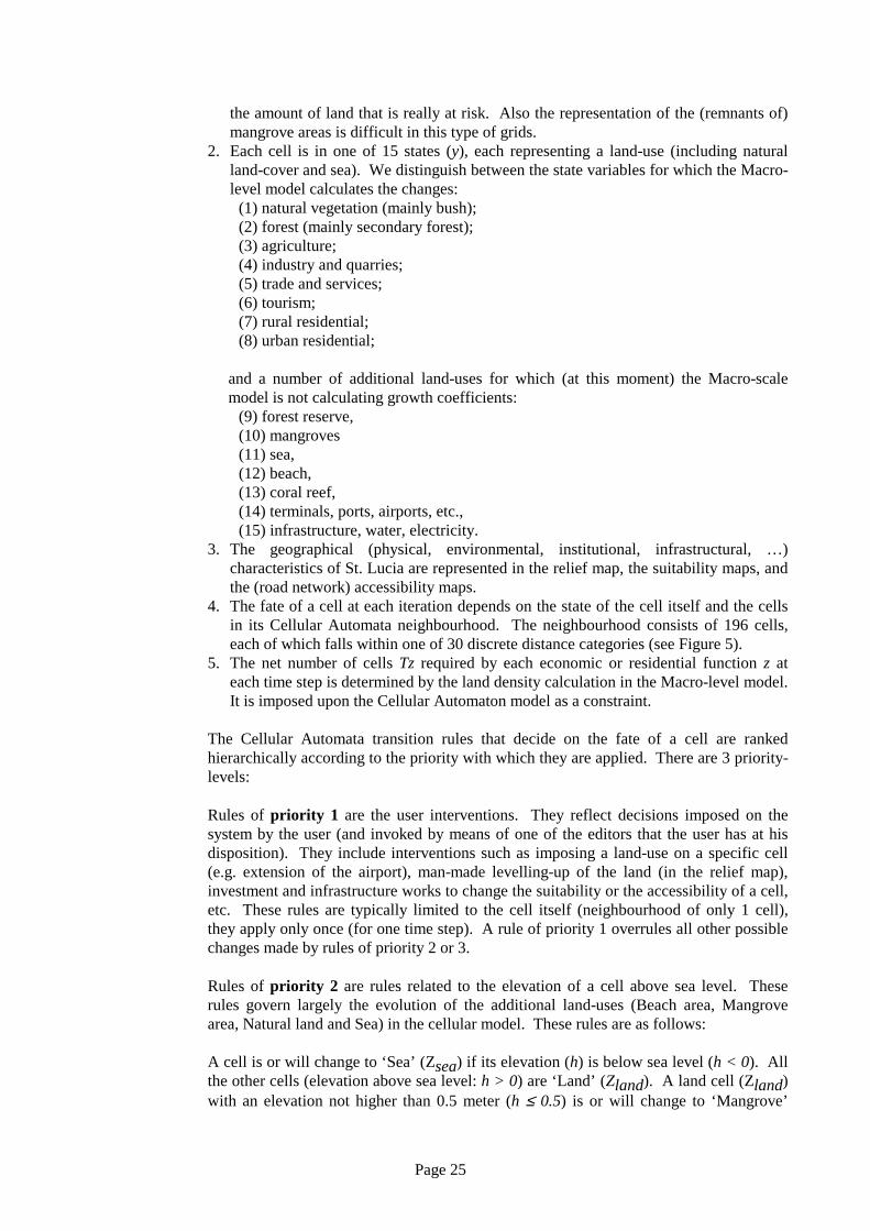
2. Each cell is in one of 15 states (y), each representing a land-use (including naturalland-cover and sea). We distinguish between the state variables for which the Macro-level model calculates the changes:
(1) natural vegetation (mainly bush);(2) forest (mainly secondary forest);(3) agriculture;(4) industry and quarries;(5) trade and services;(6) tourism;(7) rural residential;(8) urban residential;
and a number of additional land-uses for which (at this moment) the Macro-scalemodel is not calculating growth coefficients:
(9) forest reserve,(10) mangroves(11) sea,(12) beach,(13) coral reef,(14) terminals, ports, airports, etc.,(15) infrastructure, water, electricity.
3. The geographical (physical, environmental, institutional, infrastructural, …)characteristics of St. Lucia are represented in the relief map, the suitability maps, andthe (road network) accessibility maps.
4. The fate of a cell at each iteration depends on the state of the cell itself and the cellsin its Cellular Automata neighbourhood. The neighbourhood consists of 196 cells,each of which falls within one of 30 discrete distance categories (see Figure 5).
5. The net number of cells Tz required by each economic or residential function z ateach time step is determined by the land density calculation in the Macro-level model.It is imposed upon the Cellular Automaton model as a constraint.
The Cellular Automata transition rules that decide on the fate of a cell are rankedhierarchically according to the priority with which they are applied. There are 3 priority-levels:
Rules of priority 1 are the user interventions. They reflect decisions imposed on thesystem by the user (and invoked by means of one of the editors that the user has at hisdisposition). They include interventions such as imposing a land-use on a specific cell(e.g. extension of the airport), man-made levelling-up of the land (in the relief map),investment and infrastructure works to change the suitability or the accessibility of a cell,etc. These rules are typically limited to the cell itself (neighbourhood of only 1 cell),they apply only once (for one time step). A rule of priority 1 overrules all other possiblechanges made by rules of priority 2 or 3.
Rules of priority 2 are rules related to the elevation of a cell above sea level. Theserules govern largely the evolution of the additional land-uses (Beach area, Mangrovearea, Natural land and Sea) in the cellular model. These rules are as follows:
A cell is or will change to ‘Sea’ (Zsea) if its elevation (h) is below sea level (h < 0). Allthe other cells (elevation above sea level: h > 0) are ‘Land’ (Zland). A land cell (Zland)with an elevation not higher than 0.5 meter (h ≤ 0.5) is or will change to ‘Mangrove’

Page 26
(Zmangrove) if it has among its 8 nearest neighbours (N8) more mangrove cells thanbeach cells. Otherwise it is or will change to ‘Beach’ (Zbeach). A land cell with anelevation above 0.5 meter (h > 0.5) is or will change to ‘Natural’ (Znatural) or to‘Forest’ (Zforest) and will change further subject to rules of priority 3 (Equation 1). Thechoice between ‘Natural’ and ‘Forest’ is determined on the basis of the suitabilities ofthe cell. If the suitability for ‘Forest’ (Sforest) is higher than the suitability for ‘Natural’(Snatural), the cell will become ‘Natural’, if not it will become ‘Forest’:
( )
( )
( ) ( )[ ]
if h then Z
if h then if Z Z then Z else Z
if h then if S S then Z else Z
sea
mangroveN
beachN
mangrove beach
forest natural forest natural
<
≤ < >
≥ >
∑ ∑
0
0 0 5
0 5
8 8
.
.
The changes in the sea level not only alter the actual land-use of a cell, but also affect itssuitability values. In the model the suitability values for cells that rise above sea levelcan be set by the user in the ‘Land loss’ dialog. The default values are given in the tablebelow (which is a screen dump of the Land loss-dialog).
Rules of priority 3 apply to the ‘Natural’, ‘Forest’, ‘Agriculture’, ‘Industry andQuarries’, ‘Trade and Services’, ‘Tourism’, ‘Rural Residential’, and ‘Urban Residential’cells. Except for ‘Natural’, and ‘Forest’ which are the ‘no-use’ states, these are the land-uses reflecting the state variables of the Macro-scale model. Rules of priority 3 calculatefor each cell a transition potential for each activity. The transition potential is anexpression of the ‘strength’ with which a cell is likely to change state to the state forwhich the transition potential is calculated. Transition potentials are calculated asweighted sums:
( ) ( ) ( ) zd i
iddyzzzz IwAfSfP ε+×= ∑∑ ,,,.. (eq. 1)
Pz potential for transition to state z,f(Sz) function (0 ≤ f(Sz) ≤ 1) expressing the suitability of the cell for activity z,f(Az) function (0 ≤ f(Az) ≤ 1) expressing the accessibility of the cell for activity z,
( ) ( ) 0if; ,,, >×= ∑∑d i
iddyzzz IwSSf (eq. 2)

Page 27
( ) ( ) ( ) 0if;1 ,,, <×−= ∑∑d i
iddyzzz IwSSf (eq. 3)
wz,y,d is the weighting parameter applied to cells with state y in distance zone d (0 ≤ d≤ 30),
i is the index of cells within a given distance zone dId,i = 1 if the state of cell i in distance zone d = y,Id,i = 0 if the state of cell i in distance zone d ≠ y,εz is a stochastic disturbance term.
Thus, cells within the neighbourhood are weighted differently depending on their state yand also depending on their distance d from the centre cell for which the neighbourhoodis defined. Since different parameters can be specified for different distance zones, it ispossible to build in weighting functions that have distance decay properties similar tothose of traditional spatial interaction equations. To reflect the unknown factors inlocation decisions, the deterministic transition potentials are subjected to a stochasticperturbation, εz.
( )[ ]εz
arand= + −1 ln
Figure 4: A function editor is used to click-in the weighting parameters of the transitionexpression (eq.1). The graph shows the influence of the proximity of ‘Terminals, Ports, Airports,etc.’ in the possible transition of a cell to ‘Urban Residential’.
The Cellular Automata transition functions will be entered graphically by means of atool, mainly consisting of an X-Y graph, in which the user can draw, by mouse-clicking,the distance decay function defining the weight coefficients used in the calculation of theprobability for transition to any type of land-use. Figure 4 shows the tool used. Negativevalues express push factors or repulsion effects, and positive numbers express pullfactors or attraction effects. Transition weight coefficients are relative numbers. This istrue for weights defined within one transition function as well as across functions andland-uses. For example in the transition pair of Figure 4, a value -9 on the ordinate at d =2.24 has to be read as 4.11 times less important than +37 at d = 3.61. Furthermore itrepresents a repulsion rather than an attraction effect. Both values represent the totalweight accorded to the whole distance ring. Hence, the weight of -9 is the total weight ofthe 8 cells of ring 5 (the centre cell is distance ring 1), while the value +37 is the totalimportance of distance ring 9 and spread over the 8 cells (see Figure 5). The

Page 28
neighbourhood of the cellular automaton incorporates 197 cells, including the centre cell.All cells of the neighbourhood are in 1 of 30 distance rings between 0 and 8 celldiameters away from the centre.
To select the Tz cells to receive the function z at each iteration, the potentials calculatedfor all cells for transition to all states are ranked from highest to lowest. Starting with thehighest value from this list, the Tz cells with highest potentials for transition to each statez are identified and the transitions are executed. Hence, a cell will change to the state forwhich its potential is highest, unless it is not among the Tz highest potentials in whichcase it might change to a state z’ for which its potential ranks second, and so forth. Allthe cells for which potentials are not among the Tz highest for any of the z states willremain in or return to the ‘Natural’ or ‘Forest’ state.
Figure 5: Left: all cells in the Cellular Automata neighbourhood are in 1 of 30 distance rings.Right: Number of cells in each of the 30 distance rings.
3.3. GIS information in SIMLUCIA
In addition to the neighbourhood calculation, the transition potentials take also intoconsideration the intrinsic suitability of a cell as well as its accessibility.
3.3.1 The Suitability Calculation
The suitability f(Sz) of a cell is a measure of the capacity of that cell to support theactivity (land use) of type z. Suitability calculations are rather standard operations inGIS. It is a composite measure, a weighted sum or product, of a series of physical,environmental, and institutional characteristics (called factors) of each cell. Factors areunique characteristics of a cell, such as: its topography, its quality of soil, its rainfall, itssensitivity to erosion, its planning regulations, its legal restrictions on land use, etc.Most advanced GIS packages have overlay analysis or cartographic modelling techniques(see e.g. Wright, 1990) available to perform the calculations required to producesuitability maps. In SIMLUCIA, the suitability calculations have been performed bymeans of IDRISI. The data and the macros required to perform the calculation, areavailable on the SIMLUCIA diskettes. For the calculation of the suitabilities thefollowing factor maps have been retained:
(1) RELUSE.IMG Land use and vegetation (Atlas of St. Lucia 1/50.000)

Page 29
(2) LANDUSE.IMG Land use in 1990 (Atlas of St. Lucia 1/50.000; Topographicsheets of St. Lucia 1/25.000; St. Lucia Tourist Map, OrdnanceSurvey 1/50.000; Map established as part of UNDP projectSTL/001/86 National Physical Development Strategy,1/25.000; Personal observations)
(3) ELEVAT.IMG Elevation (Topographic sheets of St. Lucia 1/25.000, St.Lucia Tourist Map, Ordnance Survey 1/50.000; Imray-lolaireYachting Chart of St. Lucia, 1/72.000)
(4) SLOPEC.IMG Slopes (calculated from (3))(5) RELZONE.IMG Life zones (Atlas of St. Lucia, 1/50.000)(6) RELDIS.IMG Land Tenure (Atlas of St. Lucia, 1/50.000)(7) RELCAP.IMG Land Capability (Atlas of St. Lucia, 1/50.000)(8) RSURFACE.IMG Rainfall (Atlas of St. Lucia, 1/50.000)
Variations within a factor, such as the degrees of slope, land capability classes, etc. arereferred to as factor types. A factor map is a map showing the geographical location anddistribution of factor types for a given factor. Factor maps can be combined in variousways to generate a composite map depicting the relative capability of a cell to support aspecific land use. The technique used in SIMLUCIA is known as ‘linear combination’. Itis a common factor combination technique, which requires the analyst to define both arating table and a weighting table. The rating table depicts the relative suitability of thevarious types within a factor. For example, slopes greater than 20% are rated 0, between10% and 20% are rated 5, and less than 10% are rated 10. The weighting table depictsthe relative importance of the various factors in determining the overall suitability of thecell. For example, slope might be twice as important as the depth of the bedrock. Theratings for each type are multiplied by the weight for each factor and the result issummed. In SIMLUCIA, the suitability values are further normalised in order to obtainsuitability values that are in the range 0-10 for all suitability maps.
The table in Annex C is a Microsoft Excel Workbook named SimLucia.XLS, containingthe 8 factors that have been retained for the calculation of the suitability maps for eachland use function of the Cellular Automata model. The rows of the table represent thetypes within the factors, and the columns represent the land use functions of the model.The values in the table, are the factor type ratings. For example, row 58, column Dcontains a rating of 8 (In SIMLUCIA we work with values in the range 0 to 10) for thecapacity of a ‘Land Capability Class II’-cell to support land use ‘Agriculture’.
At the end of the table, there is a section entitled ‘Factor Weights’. This section containsthe weights accorded to each factor (and to all the types of that factor) in the finalweighting of the factors. For example the value 4 in 126, column D, means that LandCapability is considered twice as important as ‘Land elevation’ (weight 2 in row 130,column D). The values in the workbook SimLucia.XLS can be altered by the user. Inaddition to the table, it features an Excel Macro, that will generate all the files required torun the IDRISI macro named LucMac.IML. This IDRISI macro, will generate thesuitability required to run the model. To that end these maps have to be imported in themodel, as explained in the manual in Section 6.1.4.
While the model is running, the suitability values for all cells actually occupied by aparticular land use are monitored. Changes in the total and average suitability for eachland-use are passed back to the Macro-level and result in further changes in the landdensity variables. In other words, the detailed land suitabilities and land-use patterns inthe Micro-level model have their effect in processes that are modelled at the Macro-level.
Page 30
The geography at the Micro-level thus affects the global dynamics directly andcontinually.
The user can view (and edit) the different suitability maps used in SIMLUCIA.
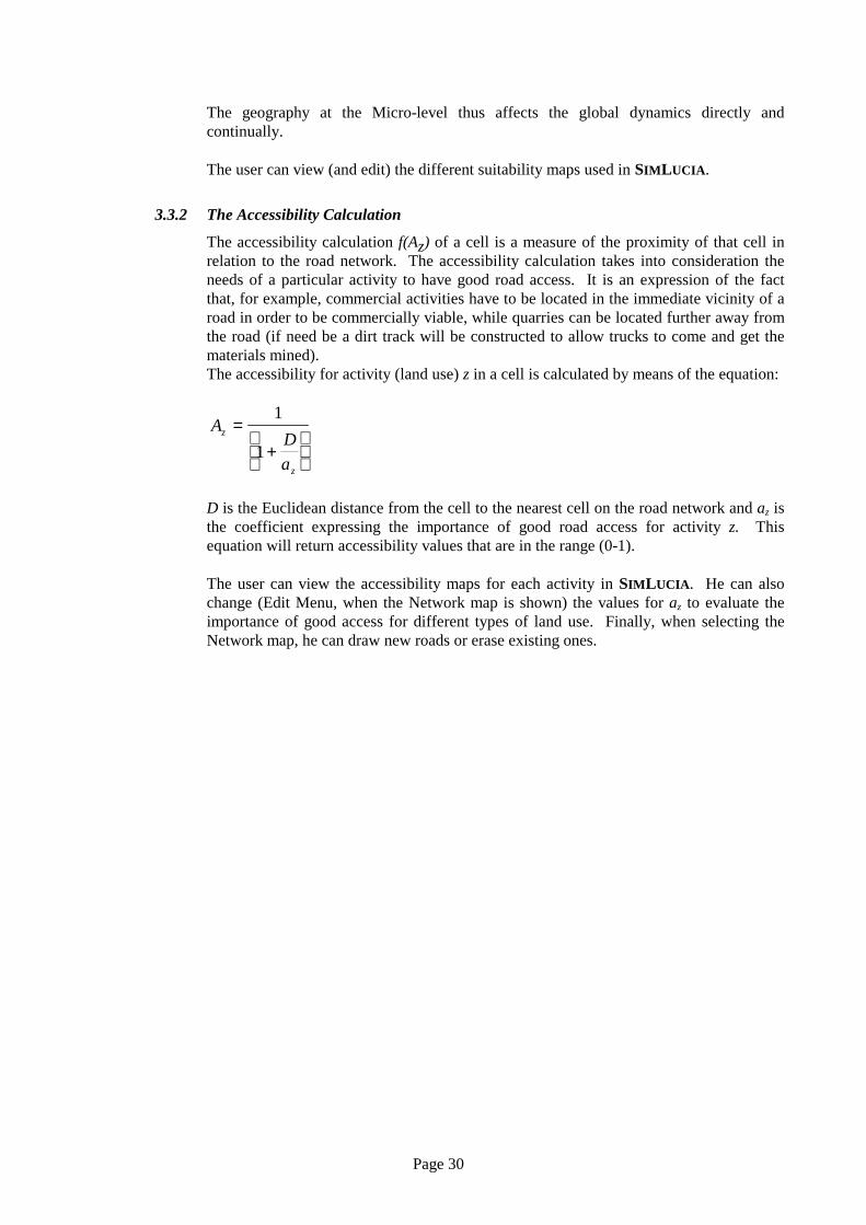
3.3.2 The Accessibility Calculation
The accessibility calculation f(Az) of a cell is a measure of the proximity of that cell inrelation to the road network. The accessibility calculation takes into consideration theneeds of a particular activity to have good road access. It is an expression of the factthat, for example, commercial activities have to be located in the immediate vicinity of aroad in order to be commercially viable, while quarries can be located further away fromthe road (if need be a dirt track will be constructed to allow trucks to come and get thematerials mined).The accessibility for activity (land use) z in a cell is calculated by means of the equation:
AD
a
z
z
=+
1
1
D is the Euclidean distance from the cell to the nearest cell on the road network and az isthe coefficient expressing the importance of good road access for activity z. Thisequation will return accessibility values that are in the range (0-1).
The user can view the accessibility maps for each activity in SIMLUCIA. He can alsochange (Edit Menu, when the Network map is shown) the values for az to evaluate theimportance of good access for different types of land use. Finally, when selecting theNetwork map, he can draw new roads or erase existing ones.

Page 31
4. Installing SIMLUCIA
This chapter explains how to install SIMLUCIA on your computer and how to start up theprogram. It also describes the main features of the user interface.
4.1. What is included in the SIMLUCIA package ?
This package consists of this printed document and two 1.44 Mb diskettes labelledSIMLUCIA disk 1/2 and SIMLUCIA disk 2/2. On SIMLUCIA disk 1/2 you will find a seriesof compressed files and 1 executable Setup.EXE that is used to install SIMLUCIA.
4.2. Installing SIMLUCIA
This section reviews the hardware and software requirements for running SIMLUCIA anddescribes the steps to install it.
4.3. Hard- and Software Requirements
SIMLUCIA runs on personal computers equipped with an Intel 80486 or Pentiumprocessor. To use the SIMLUCIA, your computer should have the following hardwarecomponents:
• At least 8 Mb of RAM (16Mb recommended)• A hard disk with at least 4 Mb free (for SIMLUCIA only)• A SVGA video card and screen (recommended: resolution 1024*768 pixels, 16
colours, size 17 inch or more) To run the applications, macro’s and exercises, which we describe and provide the filesfor on the demo diskettes, you should have the following software packages installed onyour computer: • Microsoft Windows 95 (or Windows 3.1x with Win32 version 1.3 extension)• Microsoft Excel (version 6.0) (optional)• IDRISI for Windows (version 2.0 or later) (optional)
4.4. Installation procedure for Windows 95
The following is a description of the step by step installation of SIMLUCIA. Theinstallation/un-installation of SIMLUCIA follows the standard for Windows 95. If your

Page 32
operating system is Windows 3.x then move immediately on to Section 4.5 Installationprocedure for Windows 3.x.
If you have a previous version of SIMLUCIA software installed on your machine, it isbetter to un-install it first. If you want to keep it though, make sure to put SIMLUCIA in aseparate distinct directory. During the installation you may encounter a message askingyou whether to keep certain files or replacing them. It is preferred to replace them for theuse of SIMLUCIA. Keeping the old ones may cause malfunctioning of the software.
1 Start Microsoft Windows 95.2 Insert the disk labelled "SIMLUCIA disk 1/2" into the drive.3 Click the Start button in the Windows 95 Task bar. Move the mouse pointer to the
Settings command and move on to select the Control Panel option. As a result theControl Panel Dialog box will open. Select from the list the Add/RemovePrograms by double clicking it. Next click the Install button in the Install/Uninstallview of the Add/Remove Programs Dialog box.
4 Next, the Windows 95 installation program will be started and will request you toclick the Next button until (1) the program has selected your disk drive as theinstallation medium, and (2) until it will have found on the diskette the Setup.EXEprogram for SIMLUCIA. Then, the command line "a:\setup.EXE" will appear in theedit field of the install window. Hit Finish to have the program continue theinstallation.
5 Continue clicking “Next” until the “Read Me” screen appears. Make sure to read thispage. After clicking “Next” again, a second dialog box appears asking you where toinstall SIMLUCIA. You can accept the default path which is "c:\SIMLUCIA" orreplace it in the edit box by one of your choice. You may use the “Browse” button toselect this path as well.
6 To go on, press the "Next" button. Otherwise to cancel the installation process, pressthe "Cancel" button. SIMLUCIA will ask whether you use Windows 95 or Windows3.x. Select Simlucia for Windows 95. If your PC is equipped with Windows 3.x,then follow the instructions in Section 4.5.
7 Next the installation program suggests to add SIMLUCIA to the new Program GroupSIMLUCIA. You are free to create another Group or to choose an existing one fromthe list shown.
8 From that moment the installation application is decompressing the necessary filesand puts them in the directory structure of SIMLUCIA. At a certain point in time youwill be asked to insert disk #2 in the drive. Insert at that moment the disk labelled“SIMLUCIA disk 2/2”.
9 If everything went OK, a last dialog box will inform you about the fact that theinstallation is finished. Once the installation on the hard disk is completed, theprogram creates a group named “SIMLUCIA” under the Start button and Programscommand. It contains an item labelled “SIMLUCIA”. When you double click thisitem, SIMLUCIA will be started and the “About” window will appear. Click “OK” toenter the Application Window.
4.5 Installation procedure for Windows 3.x
If you have a previous version of SIMLUCIA software installed on your machine, it isbetter to un-install it first. If you want to keep it though, make sure to put SIMLUCIA in aseparate distinct directory. During the installation you may encounter a message asking
Page 33
you whether to keep certain files or replacing them. It is preferred to replace them for theuse of SIMLUCIA. Keeping the old ones may cause malfunctioning of the software.
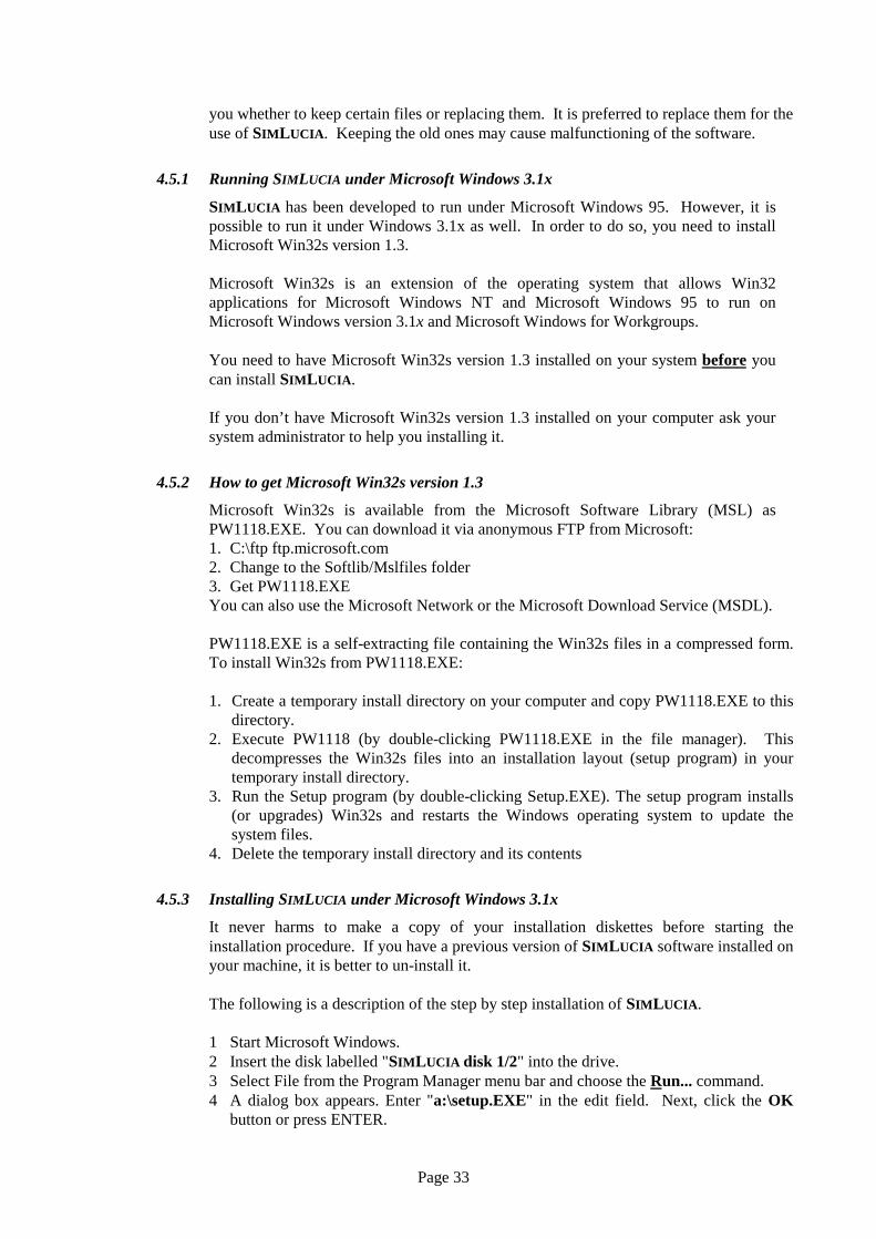
4.5.1 Running SIMLUCIA under Microsoft Windows 3.1x
SIMLUCIA has been developed to run under Microsoft Windows 95. However, it ispossible to run it under Windows 3.1x as well. In order to do so, you need to installMicrosoft Win32s version 1.3.
Microsoft Win32s is an extension of the operating system that allows Win32applications for Microsoft Windows NT and Microsoft Windows 95 to run onMicrosoft Windows version 3.1x and Microsoft Windows for Workgroups.
You need to have Microsoft Win32s version 1.3 installed on your system before youcan install SIMLUCIA.
If you don’t have Microsoft Win32s version 1.3 installed on your computer ask yoursystem administrator to help you installing it.
4.5.2 How to get Microsoft Win32s version 1.3
Microsoft Win32s is available from the Microsoft Software Library (MSL) asPW1118.EXE. You can download it via anonymous FTP from Microsoft:1. C:\ftp ftp.microsoft.com2. Change to the Softlib/Mslfiles folder3. Get PW1118.EXEYou can also use the Microsoft Network or the Microsoft Download Service (MSDL).
PW1118.EXE is a self-extracting file containing the Win32s files in a compressed form.To install Win32s from PW1118.EXE:
1. Create a temporary install directory on your computer and copy PW1118.EXE to thisdirectory.
2. Execute PW1118 (by double-clicking PW1118.EXE in the file manager). Thisdecompresses the Win32s files into an installation layout (setup program) in yourtemporary install directory.
3. Run the Setup program (by double-clicking Setup.EXE). The setup program installs(or upgrades) Win32s and restarts the Windows operating system to update thesystem files.
4. Delete the temporary install directory and its contents
4.5.3 Installing SIMLUCIA under Microsoft Windows 3.1x
It never harms to make a copy of your installation diskettes before starting theinstallation procedure. If you have a previous version of SIMLUCIA software installed onyour machine, it is better to un-install it.
The following is a description of the step by step installation of SIMLUCIA.
1 Start Microsoft Windows.2 Insert the disk labelled "SIMLUCIA disk 1/2" into the drive.3 Select File from the Program Manager menu bar and choose the Run... command.4 A dialog box appears. Enter "a:\setup.EXE" in the edit field. Next, click the OK
button or press ENTER.

Page 34
5 The screen turns blue and a second dialog box appears asking you where to installSIMLUCIA. You can accept the default path which is "C:\SIMLUCIA" or replace it inthe edit box by one of your choice.
6 To go on, press the "Next" button. Otherwise to cancel the installation process, pressthe "Cancel" button. When given a choice between installing under Windows 95 orWindows 3.1 choose the latter.
7 From that moment the installation application is decompressing the necessary files.At a certain point in time you will be asked to insert disk #2 in the drive. Insert at thatmoment the disk labelled “SIMLUCIA disk 2/2”.
8 If everything went OK, a last dialog box will inform you about the fact that theinstallation is finished. Once the installation on the hard disk is completed, theprogram creates a group named “SIMLUCIA” in the Program Manager. It contains anitem labelled “SIMLUCIA”. When you double click this item, SIMLUCIA will bestarted.
4.6. Starting SIMLUCIA
To invoke the complete environment
1 Start Microsoft Windows.2 Under the Windows 95 Start button and the Programs group, you will find a group
called SIMLUCIA. Double-click on the SIMLUCIA icon in the SIMLUCIA group.3 SIMLUCIA will be started and you will see the SIMLUCIA Application window on
your screen.
4.7. Screen Layout
When you start SIMLUCIA, you will enter immediately in the Application Window of thesimulation environment. This is the window in which you will run your models. Beforea simulation file is opened, the screen is empty except for its top part. Below we willdescribe the different components of this screen.
Application Window
Tool bar
Menu BarControl Menu Box Caption Bar
Status barApplication Window

Page 35
4.7.1 The Control Menu Box
The Control Menu box contains the Application Window Control Menu, which controlshow windows are arranged on the desktop. The list below summarises the Control MenuCommands.
Use this command ToRestore Restore the window to its previous size
Move Move the window using the arrow keys.
Size Change the size of the window. You can use the mouse or the arrow keysto change the size.
Minimize Shrink the window to an icon
Maximize Enlarge the window to the full size of the screen
Close Close the application window
4.7.2 The Caption Bar
The Caption Bar, also Title Bar, of the Application Window displays “SIMLUCIA”.
To the left of the Caption Bar three buttons are positioned that enable you to re-size theApplication window.• The Minimize button allows you to shrink the window to an icon (same as Minimize
in the Control Menu Box);• The Maximize button allows you to enlarge the application window to the full size of
the screen (same as Maximize in the Control Menu Box);• The Close button allows you to close the application window, and thus quit the
application (same as Close in the Control Menu Box)
4.7.3 The Menu Bar
The Menu Bar of the Application Window contains SIMLUCIA’s main Menu. Thecommands are logically organised in the menu so that you will quickly becomecomfortable with the various functions of the program. The menus are summarised in thetable below; subsequent chapters elaborate on the description. Chapter 6 gives anoverview of all menu commands.
Use this menu ToFile Manage your simulation files. The printing facilities are also located in this
menu, and if you want to exit the program, you can do it from here.Edit Edit the maps that are part of the Micro-scale model. All commands for
editing are located here. Depending on the type of map that is active, theappropriate edit features are listed and accessible.
View Enables to change the way a map is displayed. Commands to zoom in and outas well as commands to display information on the foreground or backgroundof the maps are part of this menu.
Maps Open a new window with one of the maps of the modelled region.
Rules Define the model at the Micro-level by means of the Cellular Automatatransition rules.
Simulation To control the simulation. The commands in this menu are the same as theones represented by means of the buttons in the Tool bar.
Options To customise the workspace. Commands permit among others to display orremove the Status bar and/or Tool bar, and to (DDE) link the simulationpackage to Excel.
Window Manage your windows on the screen
Help Invoke the on-line Help facilities.

Page 36
4.7.4 The Tool bar
The Tool bar, also known as Speed Bar, gives a faster access to some of the morefrequently used commands which are also accessible via the menu.
Use this Button ToOpen a simulation file from the disk.
Save a simulation file to disk.
Change the pointer to a pen. The pen is used to pick a value from the legendand enter it in a cell on the map.Change the pointer to a bucket. The bucket is used to pick a value from thelegend and enter it in larger, contiguous areas on the map.Change the pointer to a ruler. The ruler is used to enter detailed informationin a cell. When a cell is clicked, a dialog will open to enter the exact value.Zoom-in. Increase the size of the map on the display.
Zoom-out. Decrease the size of the map on the display.
Advance the simulation with one simulation step.
Advance the simulation till the next pause is reached (as set with the Pauses... command).Stop the simulation.
Reset the simulation. State variables of the model and maps take their initialvalues, parameters keep their actual values.To print the Micro-scale dynamics window.
Access the context sensitive help cursor. The next click action on acommand will invoke the context sensitive help on this command.
The Tool bar also displays the simulation clock. Each time step, the clock is updated.The figure indicates the years simulated in the range 0 to 40.
The Tool bar command in the View Menu allows to display or hide the Tool bar in theSIMLUCIA Application Window.
4.7.5 The Status bar
The Status bar is displayed at the bottom of the Application Window. This zoneprovides information to the user on his actions while he is working with the application.The left area of the status bar describes actions of menu items as you use the mouse orarrow keys to navigate through menus. This area similarly shows messages describingthe actions of toolbar buttons when pressed. The right area of the status bar indicateswhich of the following keys are latched down:
Indication DescriptionCAP The Caps Lock key is latched down.NUM The Num Lock key is latched down.SCRL The Scroll Lock key is latched down.

Page 37
The Status bar command from the View Menu allows to display or hide the Status bar inthe SIMLUCIA Application Window.
4.8. Getting Help
SIMLUCIA comes with a very concise on-line Help facility. Its structure and operation isin accordance with the Microsoft Help standards. Hence, using Help should pose noproblems for those familiar with Windows.
To get Help, press “F1” or the key sequence ALT-H
The Help menu has 3 items:1 “Index” gives an access to the index of the help guide.2 ”Using Help”, gives the general instructions on how to use the Windows Help
System.3 “About SIMLUCIA ...", gives information about the copy of the SIMLUCIA that you
are using.
4.9. Exiting SIMLUCIA
Closing SIMLUCIA is simply done by selecting the Exit command from the File menu. Ifyou have simulation files open when you select Exit, the application will ask whetheryou want to save simulation results. If you confirm to be interested in saving results youwill get the Save Dialog box. More information on saving simulation results is given inthe next chapter.
4.10. If you experience problems
If you experience problems in installing or running SIMLUCIA, contact:Research Institute for Knowledge Systems bv.To the attention of Inge Uljee or Guy EngelenP.O. Box 4636200 AL MaastrichtThe NetherlandsTel: +31 43 388.33.22Fax: +31 43 325.31.55E-mail: [email protected]

Page 38
5. Running SIMLUCIA Simulations
This chapter describes how to run simulations with SIMLUCIA. In the previous chapterwe explained how to install and run SIMLUCIA. We assume from now on that you haveread this information, that you have knowledge of the different technical termsintroduced, and that you have successfully installed SIMLUCIA on your computer.
5.1. Running a simulation
Click the Start button in the Windows 95 Task bar and point the cursor to the Programsgroup. Move through the cascading menu into the SIMLUCIA group and open SIMLUCIA
by clicking the SIMLUCIA icon. If the software has been installed successfully, theApplication Window will open. Immediately the About Information Window will open.Push the O.K. button (or the SIMLUCIA icon) after having read the information andwarnings in the About Window. Immediately the Open dialog box will open. If not,push the Open Simulation file button.
Look in the Open dialog box for files with a .SIM extension.
By means of the standardWindows 95 manipula-tions you can navigatethrough the directories onyour hard disk, or onanother computer in thenetwork, in search of thesimulation file of yourchoice. Once the name ofthe file appears in theOpen Dialog Box, select itand press the Open buttonor double click the fileicon.
In fact the .SIM file contains references to all the files that are required to run a model.Later in this chapter we will give more details about the contents and composition of the.SIM files.
Once all files have been loaded, two windows will appear in the Application Window:one titled Micro-scale dynamics and the other Macro-scale dynamics.

Page 39
5.1.1 The Micro-scale dynamics Window
The Micro-scale dynamics Windows is split into 3 viewing areas, called Panes. Panesare separated from one another by means of Splitter Bars. You can displace the SplitterBars to change the size of the Panes. To this end, position the cursor over the SplitterBar. The cursor changes to the Split Pointer (see Annex D for the pointer shapes). Withthe left mouse button clicked down, the Splitter Bar can be moved and the size of thePanes are adjusted accordingly.
The Pane on the left of the Micro-scale dynamics Window --called the Map pane--contains a map representation of the modelled region. More in particular the actual landuse of the region is mapped. The legend of the map is displayed in the upper left pane --called Legend pane--. The lower left Pane --called the Focus pane-- shows the mappedregion in small. In the upper part of this small map you will see a wire-frame (aninverted rectangle). This shows the area (called focus) that is displayed in the Map pane.If the mouse is placed inside this wire-frame, the frame can be moved while holding theleft mouse button clicked down. While the wire-frame is moved, you will notice that thefocus of the map in the Map pane is changing accordingly. The focus of the map canalso be changed by means of the scroll-bars of the Map pane. The Legend pane too isequipped with a vertical scroll bar.
When a simulation is running, the Micro-scale dynamics Window will be updated andthe resulting land use will be displayed in the Map pane.
The commands of the View Menu permit to change the manner in which Micro-scaleresults of the model are displayed in the Map pane. Display options include amongother: Zoom in, Zoom out, and 3-D representation. For a complete overview, consult theView Menu in Section 6.3 of this User guide.
Legend Pane
Map Pane
Focus Pane
Splitter Bar
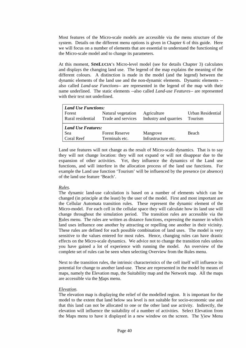
Page 40
Most features of the Micro-scale models are accessible via the menu structure of thesystem. Details on the different menu options is given in Chapter 6 of this guide. Herewe will focus on a number of elements that are essential to understand the functioning ofthe Micro-scale model and to change its parameters.
At this moment, SIMLUCIA‘s Micro-level model (see for details Chapter 3) calculatesand displays the changing land use. The legend of the map explains the meaning of thedifferent colours. A distinction is made in the model (and the legend) between thedynamic elements of the land use and the non-dynamic elements. Dynamic elements --also called Land-use Functions-- are represented in the legend of the map with theirname underlined. The static elements --also called Land-use Features-- are representedwith their text not underlined.
Land Use Functions:Forest Natural vegetation Agriculture Urban ResidentialRural residential Trade and services Industry and quarries Tourism
Land Use Features:Sea Forest Reserve Mangrove BeachCoral Reef Terminals etc. Infrastructure etc.
Land use features will not change as the result of Micro-scale dynamics. That is to saythey will not change location: they will not expand or will not disappear due to theexpansion of other activities. Yet, they influence the dynamics of the Land usefunctions, and will interfere in the allocation process of the land use functions. Forexample the Land use function ‘Tourism’ will be influenced by the presence (or absence)of the land use feature ‘Beach’.
Rules.The dynamic land-use calculation is based on a number of elements which can bechanged (in principle at the least) by the user of the model. First and most important arethe Cellular Automata transition rules. These represent the dynamic element of theMicro-model. For each cell in the cellular space they will calculate how its land use willchange throughout the simulation period. The transition rules are accessible via theRules menu. The rules are written as distance functions, expressing the manner in whichland uses influence one another by attracting or repelling one another in their vicinity.These rules are defined for each possible combination of land uses. The model is verysensitive to the values entered for most rules. Hence, changing rules can have drasticeffects on the Micro-scale dynamics. We advice not to change the transition rules unlessyou have gained a lot of experience with running the model. An overview of thecomplete set of rules can be seen when selecting Overview from the Rules menu.
Next to the transition rules, the intrinsic characteristics of the cell itself will influence itspotential for change to another land-use. These are represented in the model by means ofmaps, namely the Elevation map, the Suitability map and the Network map. All the mapsare accessible via the Maps menu.
Elevation.The elevation map is displaying the relief of the modelled region. It is important for themodel to the extent that land below sea level is not suitable for socio-economic use andthat this land can not be allocated to one or the other land use activity. Indirectly, theelevation will influence the suitability of a number of activities. Select Elevation fromthe Maps menu to have it displayed in a new window on the screen. The View Menu

Page 41
allows to change the manner in which the map is displayed. The possibility exist toZoom in, to Zoom out or to change the elevation categories with the Legend Dialog box.
Suitability.For each land-use function a suitability map is present in the model. It shows howsuitable each cell in the region is to support the particular land use. Suitabilitycalculations are rather standard GIS operations. Suitabilities are composite measures thatinvolve the manipulation of so called Factor Maps. In SIMLUCIA a linear combinationof factors has been applied: the importance of a factor type (for a specific land use) isfirst rated and next, the factors are weighted and summed. In Annex C an overview ofthe factor type ratings and factor weights is given. The calculations required to producethe suitability maps have been carried out by means of IDRISI for Windows Version 2.0(Eastman, 1997), and the resulting maps have been imported in SIMLUCIA.
The suitability map of each land use function can be selected from the Maps menu andthe way the map is displayed can be altered by means of the View and Edit menu.
Network.For each land-use function an accessibility map is present in the model. It shows howaccessible each cell is in relation to a network. The network can be --in principle atleast-- any network. In this version of the model, the network included is the roadnetwork. For some activities, such as Trade and services, the direct access to the roadsystem is more important than for other, such as Agriculture. The maps are the result ofan accessibility calculation of the parameters which are accessible via the Edit Menu.
The user can freely open and close maps (except for the land use map in the Micro-scalewindow). We warn the user that opened windows are updated while the simulation isrunning and that this does take-up processing time, hence that the program will be sloweddown.
More details on the use of Cellular Automata for modelling geographical phenomena atthe Micro-scale can be found in Chapter 3 and in the publications in the reference list.
5.1.2 The Macro-scale dynamics Window
The Macro-scale dynamics Window is thegraphical interface to the Macro-scalemodel. It shows an overview of thestructure of the system modelled at the mostsynthetic level. It allows access to all thedetails of the model at this level, but evenso at lower levels. You should learn to usethe graphical representation as a graphicalexplorer of the model.
In this prototype, the model structure, norits graphical representation can be changedby the user.
SIMLUCIA has been developed by means ofthe simulation package GEONAMICA (seeAnnex A for details). The model consists ofso-called Model Building Blocks (MBB’s)

Page 42
--the rectangles in the system diagram-- connected to one another by means of MBBConnectors --the arrows connecting the rectangles--. A MBB contains the code requiredto calculate and execute mathematical operations varying from a single operation (suchas the summation of two numbers) to a list of operations (set of mathematical equations).In order to improve the readability of the system diagram, it is possible to group parts ofthe model into a Super MBB and represent it in the diagram as a single block.
Model Building Blocks (MBB’s).The system diagram allows the user to understand the structure of the model and toaccess parts of it. Model building blocks are represented by means of a rectangle withthe name of the MBB in it.
Active Model Building Blocks appear in black on the display. When the user moves themouse pointer on top of such a MBB, its colour will invert. If the user clicks the mouse,the response will depend on the type of MBB. If the MBB clicked is not a SuperMBB,then a dialog box will open. This dialog box has the function of both receiving the dataentered by the user and of communicating model results to the user. If the MBB is aSuperMBB, then a more detailed diagram is shown in which each of the MBB’s will actas explained.
Connectors and Connections.Variables and parameters can be passed from one MBB to the other viaConnections, or Pipes. MBB’s will dispense variables or parameters withthe rest of the model via Out-connectors, and will take-in informationfrom other MBB’s via In-connectors.
The actual exchange between MBB’s is possible when a Connection (orPipe) is drawn between an Out-connector of the issuing block and the In-connector of the receiving block. For each variable or parameter that isbeing exchanged, one connection is drawn (except if one of the MBB’s isa SuperMBB) in the diagram.
Dialog boxes.Each MBB has a dialog box attached to it. This dialog box is the vehicle that permits theinteractive exchange of information between the user and the Model Building Block.The MBB will communicate the results (output) of its numerical operations to the userand it will accept the data entered (input) by the user that are required for the executionof the MBB. The latter are internal to the MBB.
Model results and model inputs are presented in Edit Fields. The difference betweeninput and output fields is indicated by the colour of the text in the edit field: green forstate variables (to be entered as initial values and for the remainder output of the MBB);purple and blue for intermediate variables; black for variables or parameters copied fromother MBB’s (output of the MBB); and finally red for internal parameters of the MBB(input for the MBB).
Colour of text in theEdit Fields ofMBB-Dialog Boxes
Description
RED Input. Parameter value (can be changed during the entiresimulation) or State variable at the initial state.
PURPLE Input. Variable value. If the edit field is clicked, a dialog willpop-up requesting input necessary for the calculation of the
In-ConnectorOut-Connector
Connection

Page 43
variableGREEN Input / Output. State variable which can be changed at the start
of the simulation, and which display output for the remainder.BLUE Output. Variable value. (read-only)BLACK Output. Values copied from other MBB’s. (read-only)
A simple way of finding out whether a field will accept input or not is by simply movingthe mouse over it. If the field can be edited, the mouse pointer will change shape infunction of the type of data that is to be entered. If the mouse is clicked, the appropriateeditor is opened. In Annex D, the meaning of the different pointers is explained.
One of four editors will open:
A single value numerical editor.
This editor allows the user to enter a single numerical value. Moreprecisely it will display a default setting --the result of thecalibration of the model-- with the request to change it with a valuewithin the range specified:
Minimum ≤ value entered ≤ Maximum
If values outside this range are entered, the user is warned.
A table (of values) editor
This editor allows the user to enter a series of numerical values. More precisely it willrequest the user to change default values. The values entered will all have to be inside arange specified:
Minimum ≤ all values entered ≤ Maximum
If values outside this range are entered, the user is warned.
A graph editor.
This editor is used extensivelyin SIMLUCIA --in both theMicro-scale and Macro-scalemodel-- to change two-dimensional relations: timeseries, distance decay functions,etc. It has two main parts: tothe left a graphicalrepresentation of the two-dimensional relation, and to theright a list box with the co-ordinate pairs defining therelation. The relation can beedited in each of the two parts.

Page 44
1. The easiest way to enter data is via direct manipulation of the graph. Move the cursorto the abscissa position for which you want to enter a new (ordinate) value. Thepointer will change to a pen symbol indicating that it is positioned correctly on top ofa vertical grid line for which it will accept an ordinate value. Move the pointer to thevertical position equal to the ordinate value which you want to enter. Then click theleft mouse button to enter the new ordinate of the point on the graph.
2 The second manner of editing is handy if you have to enter exact numbers rather thantrends or approximate numbers. It consists in clicking in the list box the co-ordinatepair that you want to change. Then a dialog box will open in which you can enter thenew ordinate value. The changes made in one part of the graph editor areimmediately visible in the other part. The number of values to be entered as well asthe range is displayed.
A Dialog editor.
In order to enter values for specific variables (printed in purple) a dialog window isopened. In this dialog the user is to enter a number of data that are required to calculatethe value of the variable. In SIMLUCIA this type of editor is used to define variables thatare required to calculate the number of jobs in each economic sector.
5.2. Starting the simulation.
Once the Micro-scale dynamics and the Macro-scale dynamics windows have beenopened, the program has read-in the default values for all the parameters as well as theinitial values for all the state variables of the model. The program is ready to run asimulation.
Verify this by pushing the Step button from the Tool bar. SIMLUCIA will now gothrough a number of essential phases (such as the initialisation and testing of itsinputs) which are of no direct interest to the user before it will make one simulationstep. This will take a while. You will notice that the action is finished when thesimulation time changes from 0 to 1 and the land-use map in the Micro-scale dynamicswindow is being updated.
Undo the simulation step by pushing the Reset button from the Tool bar. This actionwill reset all the state variables of the model to their initial value, but will not do sofor the values of the parameters. These are not influenced by Reset and remainunchanged. Since we have not changed parameter values the latter is of noimportance now, but it will be an important issue once you will be changing parametersettings while running the models.
The Micro-scale dynamics and Macro-scale dynamics Windows can not be closed by theuser (the Close-Window-icon in the Title Bar of both windows is greyed out). The usercan only minimize or maximize their size by clicking the respective icons in the TitleBar. The results of the Micro-scale models is always shown by means of the map in theMicro-scale dynamics Window. You can personalize the Micro-scale map by means ofthe command in the View and Options menu. It is possible to add overlay information toit, such as the road system and the boundaries of the administrative regions. If the regionboundaries are drawn, it is possible to pick-up information per region from the map byclicking the left mouse button in the region of your choice. An Information Window willshow an overview of the land use within the region. While the simulation is running, this

Page 45
overview is updated dynamically, thus permitting to get an impression of the changesaffecting the region.
The output of the Macro-scale models is not visible unless the user has opened the partsof the model that he wants to see. As an example we will see what the model has to offerin the Wealth MBB. Move the mouse to the MBB named Wealth. As soon as the mouseis inside the borders of the MBB, the colour of the MBB will invert. Now click the leftmouse button. The following Dialog Box will open.
Now have the simulation make one simulation stepagain while watching the values displayed in thebox. Notice that the value of the variable named“Population“ is updated whenever the nextsimulation step is taken. Finally, the Micro-scaledynamics Window is updated. This demonstratesthe fact that models developed with SIMLUCIA havecoupled micro- and macro-components runningsimultaneously. For variables preceded by a whitecheck-box, such as 'Total jobs' in the Wealth dialog,the model allows to make a time-graph. All youneed to do is to click in the check box and the graphwill open. As long as it is open, it will be updated ateach simulation time step. To close it, you shouldclick the Close-Window-icon in the title bar of theGraph window.
5.3. Viewing model output
The user of SIMLUCIA has a lot of freedom in selecting and organising the in- and outputwindows. There are tens of windows containing information related to the model. Thesewindows are all accessible in the manner explained: Macro-scale dynamics; Micro-scaledynamics; Dialog boxes; Graphs, and Maps. A window, map or dialog will be opened bythe user and will stay open until it is minimized or closed by the user. While thesimulation is running all the windows that are opened are updated. This has the greatadvantage of displaying information from linked MBB’s simultaneously and allow theuser to see how changes occur in different parts of the model.
However, the user should learn to manage output windows carefully and to close as muchas possible the windows he is not directly interested in. If not, his screen will beoverloaded with ‘left-over’ information which he is not really using, but also, everywindow opened is updated by SIMLUCIA and the act of updating takes execution timeand memory space. Hence the program might slow down considerably. Certainly whenmaps are displayed, it is imperative to close as much as possible the maps that are not ofimmediate interest to the user.
Moving the mouse with the left mouse-button clicked-down in the Title Bar of a window,will permit to move it around. It is good practice to organise the screen in such a waythat the dialogs are all grouped on one side of the screen and the map(s) on the other side.This will permit to see simultaneously macro- and microscopic results of the simulations.

Page 46
5.4. Saving simulation results
Working with Decision Support Systems is not in the least a learning process: thedecision maker is exploring different combinations of policy alternatives to learninteractively which interventions are likely to satisfy his policy criteria. Theseexplorative exercises require a possibility to store simulation results in an efficientmanner.
The Save simulationcommand fromSIMLUCIA’s File menuallows the user to storesimulation results in moreor less sophisticatedmanners. More inparticular it allows theuser to manage efficientlythe different kind of filesthat constitute a singlesimulation. Indeed, asimulation requires notjust one, but 10 to 20 datafiles, hence, saving a largenumber of simulation runsmight require a largestorage space on your harddisk(s).
When the user selects Save Simulation from the File menu, the Save Dialog box willopen, requesting the user to enter the name of the file. If the name of the currentsimulation file is entered, then it will be overwritten, and the original values will be lost.Overwriting files can be avoided by simply choosing a file name different from thecurrent one. Once the name of the file is entered and the Save button has been pressed,the system will display the Simulation file ... .SIM Dialog box. If you are a relativelynew user of SIMLUCIA, simply press the OK button to complete the action of saving thesimulation and skip the remainder of this section. If however, you are more experiencedwith the system this Dialog box will help you to change the composition of yoursimulation file before saving it.

Page 47
The dialog box shows anoverview of all the filestypes --and theirrespective names-- thatare used by the simula-tion. In the box, the filesare preceded by a checkbox. Files preceded by acrossed check box will besaved with the namementioned to their right.The program keeps trackof the actions that the userhas performed during asession and knows whatfiles are affected by it.
These files are shown with their check-box crossed, and that is why the program suggeststo save them. If however you do not want a new copy --for example because thecorrections you made are not important-- then you simple cross out the check box.Although this procedure might seem cumbersome at first, it will become a great help toyou once you are more familiar with the system. SIMLUCIA saves its output in exactlythe same format as its inputs. Hence, you can always use saved simulations as the inputfor a new run. Keep in mind however that the simulation clock will be set back to 0when you continue a simulation in this way.
Save simulation will only save final results of the model (current values of state variablesand parameters). It will not store intermediate results. To save these, you should makeuse of the Log ... and the Link to Excel commands from the Options menu.
Log ... will save Micro-scale simulation results. More in particular it will store maps ona .LOG file. When the Log ... command is selected, the user will have to enter theinterval for which he wants to store maps.
The Link to Excel command permits to send simulation data to a Microsoft ExcelWorkbook. More in particular the values of a number of the most important statevariables will be send to Excel. It is possible to save this Workbook (using the Excelcommands) and thus store them for further analysis.
5.5. Printing simulation results
Printing simulation results can be done in different manners. SIMLUCIA supports verydirectly the printing of maps. From the File menu, you will use the commands PageSetup, Print preview and Print for that matter. Select first Page Setup to decide on thenumber of cells which you want to print out per unit of measurement (for example 4 cellsper cm for a map of St. Lucia at a scale of 1/100.000), then select Print Preview to get anidea on how the printed maps will look like, and finally push the Print button in the PrintPreview window or from the Tool bar to print the maps.
Printing results from the Macro-level model can be done by selecting Link to Excel fromthe Options menu and use the Excel print functions to get the results on paper. If you

Page 48
want a printout from a particular MBB, then click it to open its Dialog box. Once theDialog box is open, key-in Alt + Prt Sc. This will put the Dialog on the WindowsClipboard. Now open your Paintbrush, Paint or Word Processing package and selectPaste from its Edit menu. Once the Dialog window has been pasted, Print the dialog byusing the print facilities of the receiving package. This procedure works not only fordialogs, but for all SIMLUCIA’s windows. It is handy to print among other the 3 Drepresentation of the study area.
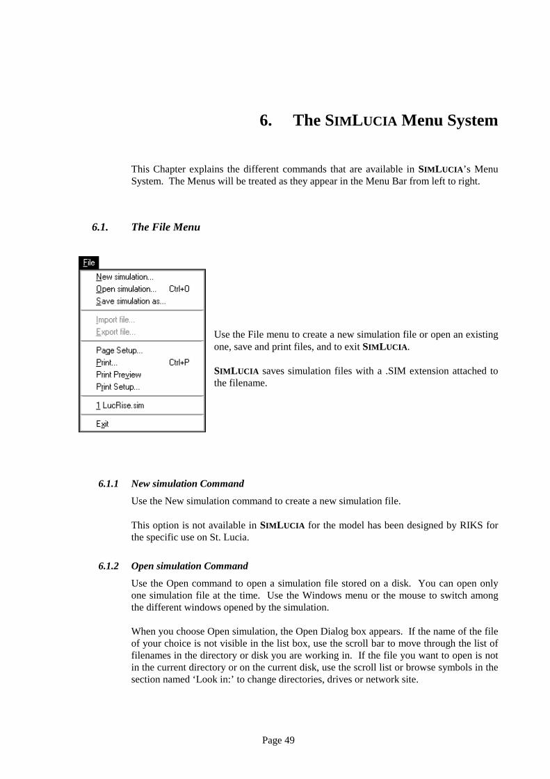
Page 49
6. The SIMLUCIA Menu System
This Chapter explains the different commands that are available in SIMLUCIA’s MenuSystem. The Menus will be treated as they appear in the Menu Bar from left to right.
6.1. The File Menu
Use the File menu to create a new simulation file or open an existingone, save and print files, and to exit SIMLUCIA.
SIMLUCIA saves simulation files with a .SIM extension attached tothe filename.
6.1.1 New simulation Command
Use the New simulation command to create a new simulation file.
This option is not available in SIMLUCIA for the model has been designed by RIKS forthe specific use on St. Lucia.
6.1.2 Open simulation Command
Use the Open command to open a simulation file stored on a disk. You can open onlyone simulation file at the time. Use the Windows menu or the mouse to switch amongthe different windows opened by the simulation.
When you choose Open simulation, the Open Dialog box appears. If the name of the fileof your choice is not visible in the list box, use the scroll bar to move through the list offilenames in the directory or disk you are working in. If the file you want to open is notin the current directory or on the current disk, use the scroll list or browse symbols in thesection named ‘Look in:’ to change directories, drives or network site.
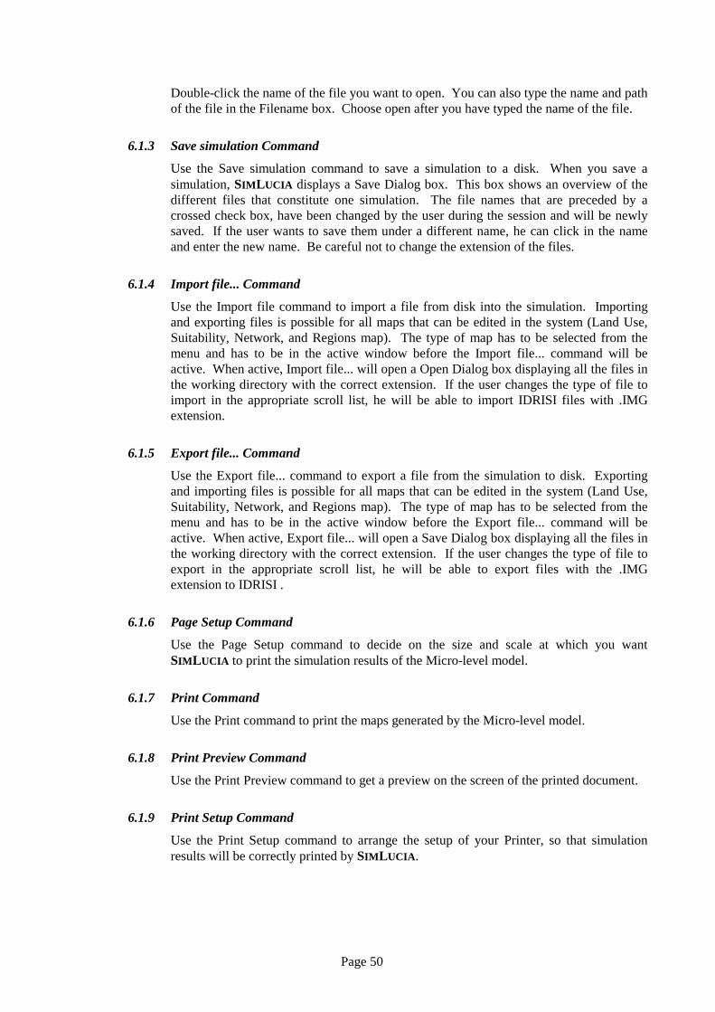
Page 50
Double-click the name of the file you want to open. You can also type the name and pathof the file in the Filename box. Choose open after you have typed the name of the file.
6.1.3 Save simulation Command
Use the Save simulation command to save a simulation to a disk. When you save asimulation, SIMLUCIA displays a Save Dialog box. This box shows an overview of thedifferent files that constitute one simulation. The file names that are preceded by acrossed check box, have been changed by the user during the session and will be newlysaved. If the user wants to save them under a different name, he can click in the nameand enter the new name. Be careful not to change the extension of the files.
6.1.4 Import file... Command
Use the Import file command to import a file from disk into the simulation. Importingand exporting files is possible for all maps that can be edited in the system (Land Use,Suitability, Network, and Regions map). The type of map has to be selected from themenu and has to be in the active window before the Import file... command will beactive. When active, Import file... will open a Open Dialog box displaying all the files inthe working directory with the correct extension. If the user changes the type of file toimport in the appropriate scroll list, he will be able to import IDRISI files with .IMGextension.
6.1.5 Export file... Command
Use the Export file... command to export a file from the simulation to disk. Exportingand importing files is possible for all maps that can be edited in the system (Land Use,Suitability, Network, and Regions map). The type of map has to be selected from themenu and has to be in the active window before the Export file... command will beactive. When active, Export file... will open a Save Dialog box displaying all the files inthe working directory with the correct extension. If the user changes the type of file toexport in the appropriate scroll list, he will be able to export files with the .IMGextension to IDRISI .
6.1.6 Page Setup Command
Use the Page Setup command to decide on the size and scale at which you wantSIMLUCIA to print the simulation results of the Micro-level model.
6.1.7 Print Command
Use the Print command to print the maps generated by the Micro-level model.
6.1.8 Print Preview Command
Use the Print Preview command to get a preview on the screen of the printed document.
6.1.9 Print Setup Command
Use the Print Setup command to arrange the setup of your Printer, so that simulationresults will be correctly printed by SIMLUCIA.

Page 51
6.1.10 List of Recent File (1, 2, 3, 4)
SIMLUCIA keeps track of the 4 most recent files opened by the program. It will displaythose in the File menu. If you select one of the 4 files, it will be opened.
6.1.11 Exit Command
Use the Exit command to quit SIMLUCIA and return to Windows.
If you have made changes to simulation files since the last time that you saved thesimulation, a dialog box appears asking whether you want to save the simulation filebefore exiting SIMLUCIA.

Page 52
6.2. Edit Menu
Use the commands on the Edit menu to edit the maps of the Micro-scale models.The first three commands on the Edit menu are standard, but for each type of mapone or more commands will be added to permit specific edit operations. These willbe explained in more detail in the Map menu.
Be careful, SIMLUCIA in not equipped with the an Undo command. Hence allcorrections made are definite !
6.2.1 Pen Command
Use the Pen command to pick a value from the legend of the map (by clicking the radiobutton next to a reading) and enter it in the map by clicking the cell of your choice.
This command will change the pointer in a pen. It is identical to selecting the Pen iconfrom the Tool bar.
6.2.2 Fill Command
Use the Fill command to pick a value from the legend of the map (by clicking the radiobutton next to a reading) and enter it in larger, contiguous areas of the map. The Fillcommand will change the values all contiguous cells that have the same colour as the onethat is clicked. It will give them the value selected from the legend.
This command will change the pointer in a bucket. It is identical to selecting the Bucketicon from the Tool bar.
6.2.3 Precision Command
Use the Precision command on the Edit menu to enter detailed information on a cell bycell basis. When a cell is clicked, a dialog will open to enter the exact value.
This command is identical to selecting the Ruler icon from the Tool bar.

Page 53
6.3. View Menu
Use the View menu to change the manner in which the different maps of theMicro-scale model are displayed. The first three commands on the Edit menu arestandard, but for each type of map one or more commands will be added to specifyviews. These will be explained in more detail in the Map menu.
6.3.1 Go to... Command
Use the Go to... command to move the cursor to a specific location on the map. Selectingthis command from the View menu will open a dialog box requesting to enter the co-ordinates of the location.
6.3.2 Zoom in Command
Use the Zoom in command to increase the size of the map on your screen by a factor 2.This command is identical to selecting the Zoom-in icon from the Tool bar.
6.3.3 Zoom out Command
Use the Zoom out command to reduce the size of the map on your screen by a factor 2.This command is identical to selecting the Zoom-out icon from the Tool bar.
When the Micro-scale dynamics Window is the active window, theView menu is completed with four additional commands: Showregions, Show transportation network, Show elevation and 3D settings.These commands allow the user to draw overlay information on top ofthe Micro-scale simulation window.
6.3.4 Show regions Command
Use the Show regions command to draw (or remove) the boundaries of the regions, asdefined in the regions map, on top of the land uses in the Micro-scale dynamics window.
6.3.5 Show network Command
Use the Show network command to draw (or remove) the network, as defined in thenetwork map, on top of the land uses in the Micro-scale dynamics window.
6.3.6 Show elevation Command
Use the Show elevation command to change the flat land use map of the Micro-scaledynamics window into a 3 D representation. The relief of this representation is asdefined in the elevation map.

Page 54
6.3.7 3D settings Command
Use the 3D settings command to change the manner in which the 3D diagram isrepresented. When this command is selected, the user will get a Dialog box allowing himto specify the angle of rotation, the perspective and the vertical exaggeration of thediagram.
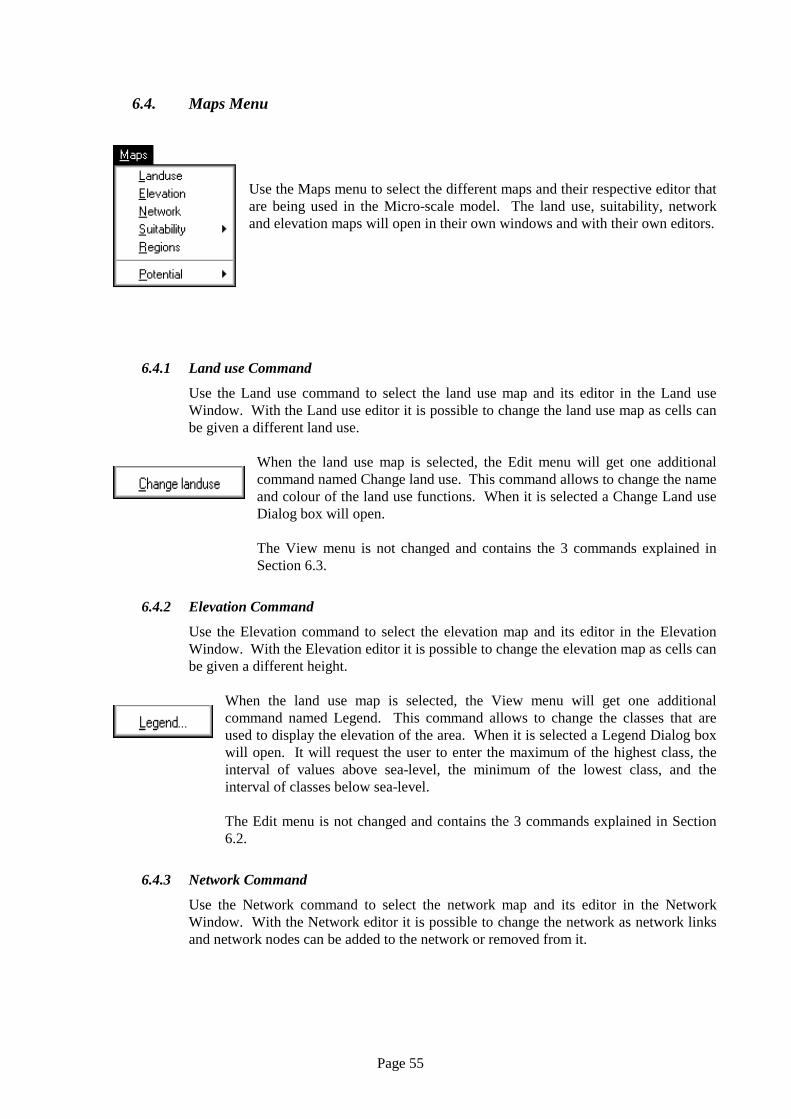
Page 55
6.4. Maps Menu
Use the Maps menu to select the different maps and their respective editor thatare being used in the Micro-scale model. The land use, suitability, networkand elevation maps will open in their own windows and with their own editors.
6.4.1 Land use Command
Use the Land use command to select the land use map and its editor in the Land useWindow. With the Land use editor it is possible to change the land use map as cells canbe given a different land use.
When the land use map is selected, the Edit menu will get one additionalcommand named Change land use. This command allows to change the nameand colour of the land use functions. When it is selected a Change Land useDialog box will open.
The View menu is not changed and contains the 3 commands explained inSection 6.3.
6.4.2 Elevation Command
Use the Elevation command to select the elevation map and its editor in the ElevationWindow. With the Elevation editor it is possible to change the elevation map as cells canbe given a different height.
When the land use map is selected, the View menu will get one additionalcommand named Legend. This command allows to change the classes that areused to display the elevation of the area. When it is selected a Legend Dialog boxwill open. It will request the user to enter the maximum of the highest class, theinterval of values above sea-level, the minimum of the lowest class, and theinterval of classes below sea-level.
The Edit menu is not changed and contains the 3 commands explained in Section6.2.
6.4.3 Network Command
Use the Network command to select the network map and its editor in the NetworkWindow. With the Network editor it is possible to change the network as network linksand network nodes can be added to the network or removed from it.

Page 56
When the network map is selected, the Edit menu will get twoadditional commands named: Accessibility parameters and Computeaccessibility.When Accessibility parameters is selected, an Accessibility parametersDialog box will open which will request the user to enter a number perland use function, reflecting the sensitivity of the function to goodaccess to the network.When Compute accessibility is selected, new accessibility values percell and per land use function are calculated. Compute accessibilityshould be invoked every time the accessibility parameters have beenchanged, or when the network has been changed.
When the network map is selected, the View menu will get anumber of additional commands. These permit to change thebackground colour of the network map. Backgrounds will eitherbe blank (White background), the actual land use (Land use, thestandard option), or the accessibility for one of the land uses.
6.4.4 Suitability Command
Use the Suitability command to select one of the suitability maps and its editor in theSuitability Window. With the Suitability editor it is possible to change the suitabilitymap as cells can be given a different suitability value.
When a suitability map is selected, the View menu will get one additionalcommand named Show features. This command allows to display the cellsoccupied by a land use feature by means of a special symbol. These cells arenot available for the allocation of functions (because they are treated as staticland uses in the model).
6.4.5 Regions Command
Use the Regions command to get a display of the Regions map in the Regions Window.The Regions map shows the different geographical entities for which the model willgenerate regional sums. The Regions map can not be changed by the user.
When the Regions map is selected, the Edit menu will get one additionalcommand named Indicator... When this command is clicked, a Dialog box willopen requesting the user to enter a weight for each land use. These weights aremultiplied with the total number of cells of that type and presented in theinformation window which can be opened by clicking in a region. Thus, thenumber of cells can be translated in another measure (i.e. if the component isthe surface of a cell in ha, the totals generated will be the area in ha taken in bythe land use function.)

Page 57
6.4.6 Potential Command
Use the Potential command to select one of the Potential maps in the Potential Window.The Potential maps are displaying the transition potential of a cell to change to the landuse specified. It is on the basis of transition potentials that each cell will get a new landuse in the next simulation step.
When a potential map is selected, the View menu will get one additionalcommand named Show function. This command allows to display the cellstaken in by the land use function for which the potential is displayed on themap. It allows the user to get an idea to what extent the land use function isindeed present in high potential cells.

Page 58
6.5. Rules Menu
Use the Rules Menu to view or enter the forces that specify the spatialinteraction of each possible pair of land uses.
6.5.1 (land use) Command
Select from the menu the land use function (LU1) for which you would like to enter, editor view its interaction with another land use (LU2). Select this other land (LU2) use bypointing at it in the cascading menu that will open and by clicking it. As a result theGraph editor will open. From its title bar you will read what interaction is to be entered:‘Effect of (land use LU2) on (land use LU1)’.
6.5.2 Overview Command
Use the Overview command to get an overview of the complete set of interaction rulesdefined in the model. The colours representing the different land uses are the same asthose in the Micro-scale window.

Page 59
6.6. Simulation Menu
Use the Simulation menu to control the simulation.
6.6.1 Init Command
Use the Init command to initialise the simulation. After the model has been initialised allthe variables display the correct initial condition (values) of the model. If the Step orRun command is selected the simulation will be automatically initialised if this has notbeen done manually.
6.6.2 Step Command
Use the Step command to advance the simulation with one step. This command isidentical to clicking the Step button from the Tool bar. Once the model has beeninitialised all the windows display the correct initial condition (values) of the model. Ifthe Step or Run command is selected the simulation will be automatically initialised ifthis has not been done manually.
6.6.3 Run Command
Use the Run command to advance the simulation till the next pause tab has been reached.This command is identical to clicking the Run button from the Tool bar. Once thesimulation is running, it can be halted by the user by selecting the Stop command fromthe Simulation Menu or by pressing the Stop button from the Tool bar. The defaultsimulation run will take 40 years. The Macro-model and Micro-model are updated on ayearly basis.
6.6.4 Stop Command
Use the Stop command to interrupt the simulation. This command is identical to clickingthe Stop button from the Tool bar. Once interrupted, the simulation will halt till the userselects the Step or Run command from the Simulation Menu or till the Step or Runbutton from the Tool bar is pushed.
6.6.5 Reset Command
Use the Reset command to reset the simulation to the initial state. This command isidentical to clicking the Reset button from the Tool bar. Selecting Reset will set thesimulation clock equal to 0. The state variables and maps are set equal to their initial

Page 60
values (hence the changes made during the simulation are lost); and the parameters keeptheir actual value.
6.6.6 Pauses ... Command
Use the Pauses... command to set the pause tabs of the simulation. When Pauses ... isselected, a Dialog box will open requesting the user to enter the time interval (in years)for which he wants the simulation to halt.
6.6.7 Random ... Command
Use the Random ... command to run the simulation in stochastic mode. When Random ...is selected, a Dialog box will open requesting the user to set a value for the εz parameteras well as the seed value for the random generator (see Chapter 3 for more on this).

Page 61
6.7. Options Menu
Use the Options Menu to personalise your workspace.
6.7.1 Grid ... Command
Use the Grid ... command to draw a (major) grid in the maps. When Grid is selectedfrom the Options menu, a Dialog box will open. The user is requested to switch on or offthe Major grid check box. Next he is to enter the size of the grid expressed in number ofcells. Finally he can offset the origin of the grid by a certain amount of cells (forexample in order to fit a reference system of some sort).
6.7.2 Font ... Command
Use the Font ... command to change the font, font style and font size of the character setused to print the legends of maps and the informative windows.
6.7.3 Link to Excel … Command
Use the Link to Excel command to link the simulation with the Microsoft ExcelWorkbook SIMLUCIA.XLS. This link is a DDE (Dynamic Data Exchange) link. Viathis link SIMLUCIA is sending model output to the Workbook while the simulation isadvancing. Note that in order to establish a successful link, it is required that Excel isinstalled on your machine and that Excel appears in the PATH statement of yourAUTOEXEC.BAT. If SIMLUCIA can not find Excel, the menu option will be greyedout. The Workbook SIMLUCIA.XLS is at the disposal of the user once the simulation isfinished. It can be used for further analysis of the simulation data.
6.7.4 Log ... Command
Use the Log ... command to store the land use maps produced by the Micro-level modelin a file. When Log ... is selected, a dialog box will open requesting the user to enter thename of the .LOG file and the interval for which simulation results are written to the file.
.LOG files can be analysed by means of the ANALYSE utility program (see Section 7).
6.7.5 Tool bar Command
Use the Tool bar command to view or hide the Tool bar in the Applications window.

Page 62
6.7.6 Status bar Command
Use the Status bar command to view or hide the Status bar in the Applications window.

Page 63
6.8. Window Menu
Use the Window menu to arrange the contents of the screen and toactivate one of the opened windows.
6.8.1 Cascade Command
Use the Cascade command to arrange multiple opened windows in an overlapped fashionso that the Title bar of each window is visible.
6.8.2 Tile Horizontal command
Use the Tile Horizontal command to vertically arrange multiple opened windows in anon-overlapped fashion so that all windows are visible.
6.8.3 Tile Vertical Command
Use the Tile Vertical command to arrange multiple opened windows side by side in anon-overlapped fashion so that all windows are visible.
6.8.4 Arrange Icons Command
Use the Arrange Icons command to arrange the icons for minimized windows at thebottom of the screen. If SIMLUCIA’S windows are positioned at the bottom of thescreen, then they can hide some or all of the icons.
6.8.5 Close windows Command
Use the Close windows command to close all the opened windows except for the onesthat can not be closed (in particular the Micro-scale dynamics and Macro-scale dynamicswindows).
6.8.6 List of Windows (1, 2, 3, 4, ...)
At the bottom of the Windows menu a list of open windows is presented. A check markappears in front of the document name of the active window. Choose a name from thislist to make the window active.

Page 64
6.9. Help Menu
Use the Help menu to select the type of Help you want SIMLUCIA to display onthe screen. The different commands in this menu will permit to look upinformation about SIMLUCIA, its commands, options, and tools.
In this version of SIMLUCIA the on-line Help is very incomplete.
6.9.1 Index Command
Use the Index command to get the opening screen of the Help file of SIMLUCIA. Fromthe opening screen, you can jump to step-by-step instructions for using SIMLUCIA.Double click the topic you want help on. A Help screen will appear. Once you openHelp, you can click the contents button whenever you want to return to the openingscreen.
6.9.2 Using Help Command
Use the Using Help command for getting general instructions on how to use theWindows Help System.
6.9.3 About ... Command
Use the About ... command to get the copyright notice and version number of theSIMLUCIA application which you are using. The latter is important if you needassistance with the software from the developers or when you request an update of thesoftware.

Page 65
7 ANALYSE
The program ANALYSE, which is also on the SIMLUCIA Demo diskette, can be used toanalyse .LOG files created with SIMLUCIA. To run ANALYSE click on the Start buttonin the Windows Task bar, move to the SIMLUCIA Programs Group and finally select theANALYSE icon.
7.1 Basic concepts and features
A .LOG file consists of a sequence of maps generated by a simulation. The name of amap in such .LOG file consists of the concatenation of the name of the .LOG file and theiteration number of the simulation. With ANALYSE you are able to compare any twomaps within the .LOG file, and see the differences expressed graphically on a map aswell as in numbers presented in a table. Also the comparison of maps from different.LOG files is possible.
The ANALYSE window has a menu bar with the menus: File, Options, Colours andHelp.
The File menu contains commands to Open and Close .LOG files, to Print the contents ofthe Application Window, and to Exit. Select Open to open a .LOG file. If there isalready a .LOG file open, the program will append (up to a maximum of 42 maps) the

Page 66
maps of the newly opened file to the current list. Thus you will have the possibility ofcomparing maps from different simulation runs. Select Close to close all the .LOG filesopened. Select Print to send the contents of the ANALYSE window to the default printerusing the default printer setup of your Windows environment. Select Exit to quit theprogram.
The Options menu gives you the possibility to overlay a grid on the map (select Showgrid/Hide grid), to represent each cell by a circle instead of a square (selectCircle/Square), and to hide or show the legend (select Hide legend/Show legend).
The Colours menu allows you to change the colours of all the features and functions thatare displayed on the map. The Colours menu will only be accessible when maps aredisplayed in the Application Window.
The Help menu only contains an About option.
Just underneath the menu bar there is a Tool bar. It contains three list boxes and fourpicture buttons.• Pushing the first button will display the map selected in the first (left) list box• Pushing the second button will display the map selected in the second (middle) list
box.• Pushing the third button will display differences between the two maps selected in
the first (left) and the second (middle) list box. Differences are displayed for theland-use selected in the third (right) list box. The comparisons are made on a cell bycell basis.
• Pushing the fourth button will display the differences between the two mapsselected in the first and the second list box by means of a matrix-like numericaloverview.

Page 67
The Kappa statistic is a measure of the resemblance of both maps compared, globallyor per land-use.
Page 68
8. Policy exercises with SIMLUCIA
Now that the general functionality of SIMLUCIA has been covered, this chapter willbriefly describe how to run simulations with SIMLUCIA and how to use it for Decisionand Policy support. We will treat three rather theoretical exercises that get progressivelymore complex and require a better understanding of SIMLUCIA.
8.1 Introduction
Policy making and more generally Decision making is a stepwise process. In order tocome to a decision, the steps are run through sequentially in one or more iteration.Depending on the author or the literature that is consulted, the process is a subdivided inmore or less phases (or steps) and different names are given to each phase. Someagreement seems to exist about the following three major phases, and their contents:• the identification phase, the purpose of this phase is to better discern the real problem
which requires a decision to be taken. This is an analytical phase during which thereal origin of a problem is the topic of research, before suggestions to solve theproblem are made.
• the development phase, this is the phase during which a more or less large number ofalternative solutions for the problems are developed.
• the selection phase, is finally the phase during which the ‘least unfavourable’ solutionamong all alternative solutions is searched for and selected for implementation.
Although the three phases have been discribed in a sequential order, it should be statedclearly that decision making is very often a cyclical process, during which some if not allof the phases are run through a number of times. The purpose of these cycles is clearly:(1) to get an in depth understanding of the real problems; (2) to generate more and bettersolutions, and (3) to decide upon an intervention or a combination of interventions thatwill solve the problem, at least in part.
Full fetched Decision Support Systems (DSS) will support the decision maker in each ofthe three phases mentioned. However many so-called Decision Support Systems willfocus on one or two of the phases only. For example quantitative models are used togenerate alternative solutions during the development phase, while multi-criteria analysisis used to select among alternative solutions in the selection phase.
This version of SIMLUCIA provides support for both the first and the second phase.SIMLUCIA will help the user to get a better understanding of the origin of problems asthey exist in St. Lucia or as they might pop-up in a more or less distant future and it willsupport the user in the design and evaluation of alternative solution to cope with theseproblems. The selection phase is less well supported in SIMLUCIA, since there is lessfunctionality built-in to compare and rank alternative solutions, other than what isavailable in ANALYSE, Microsoft Excel or IDRISI.
Page 69
In the three exercises we will study the effects of external factors and policyinterventions. The exercises have been kept rather simple. Their purpose is mainly tomake you acquainted with SIMLUCIA to the point that you will be able to run your ownexercises. First we will show how to study the effects of external factors. Next we willsee how interventions of the type ‘policy interventions’ can be tested with the system.
If you intend to use SIMLUCIA for planning or policy making, you should remember thatyou are working with a model and that this particular model is a strong simplification ofreality (see chapters 2 and 3). More, SIMLUCIA is an instrument intended for scientificanalysis, hence, you have full access to nearly all of its parameter and variables.Whenever you change parameters or variables beyond their validity interval, the modelmight generate results that are merely nonsense. In conclusion, use the model in aresponsible manner and with particular care !
All the exercises in this chapter will be done with the simulation files namedLucNoCh.SIM and LucRise.SIM. In the chapters 4 and 5 we have explained how to StartSIMLUCIA, how to Open a simulation and how to Run, Reset and Exit a simulationexercise. We assume that you know all this at this point. Begin each of the exercisesdescribed underneath by starting SIMLUCIA.
8.2 Exercise a: Working with scenarios
The effectiveness of planning can be strongly influenced by physical, economic andsocial factors external to the system. They are usually beyond the control of the planneror policy maker. His intervention is limited to the early detection of possible dangerscaused by these factors and the design and implementation of counter measures. In orderto select appropriate and robust measures, he will introduce external factors as scenariosin the system and study the behaviour of the system and its response to these newconditions.
In SIMLUCIA Change in temperature and Change of the sea level are external factors,because it is very unlikely that local decision makers can directly influence these.
Aim: In this exercise we want to examine the effects of temperature rise and sea levelrise on the loss of land and its further consequences on the tourism sector.
Screen arrangement: We will arrange the screen layout in such a manner that the inputand output windows of the model which are most relevant to this exercise are on thedisplay. This does not mean that the other windows are irrelevant. Because SIMLUCIAis a highly integrated model, most state variables will undergo some changes as a resultof the exercise. Hence, feel free to dig deeper into the model to discover other effects ofthe scenarios that we will simulate.• First open the simulation file called LucNoCh.SIM;• Minimize the Micro-scale dynamics window;• In the Macro-scale dynamics window, click the MBB called ‘Climate’. The Climate
window will open. Move it to the left (top) side of the display;• In the Macro-scale dynamics window, click the MBB called ‘Land use’. Move the
Land use Dialog window to the right (top) side of the screen;• In the Macro-scale dynamics window, click the MBB called ‘Labour’. In the
Economic Sub-system dialog window, click the edit field in the column ‘Tourism’and the row ‘Labour’. As a result a new dialog window will open named Jobs:

Page 70
Tourism. Move this window to the right side of the screen, position it below the Landuse dialog window, and click the check box left of the text Jobs. As a result a graphwill open named ‘Jobs: Tourism’;
• now minimize the Macro-scale dynamics window;
It is good practice to manage your windows very carefully. This will keep you frombeing distracted. Keep only the windows opened that are of direct interest to you. Allwindows and dialogs that are open are updated by the program, even if they are hidden byother windows. This takes execution time and memory space, and thus will slow downthe program.
As a result of the above actions, your Application window should look more or less likethis:
What-if? simulation: We will compare two scenarios: the first with no climate change,the second with a temperature rise of 2°C and sea level rise of 0.8 foot in 40 years(between 1990 and 2030). The first scenario is a so-called ‘business as usual’ scenariowhich we will use to establish a reference state, the second is a scenario which is withinthe limits of scenarios presented recently (see for example: Maul, 1993)
Press the Run button in the toolbar to start the simulation. In the Climate window, noneof the values will change (as we assume no climate change in this first run). In the Landuse window you will see how the number of cells for each land use are changing. Thesechanges are due to the population dynamics and the external demand for goods producedby the different economic sectors. Notice for instance how natural vegetation and forest

Page 71
is gradually losing cells as the simulation proceeds. Notice also that the tourism sector isexpanding and new cells are taken in by tourism activity. This growth is also visible inthe Jobs: Tourism dialog and graph.
When the simulation comes to a halt (after 40 years), push the Reset button. Then clickthe Restore button in the title bar of the (minimized) Micro-scale dynamics window. Asa result the window will open. Run the simulation again and see how the land use ischanging. Remember that these changes are simply due to the demographic pressure andexpansion of the economic sectors. Notice for instance the fast expansion of theindustrial area near Vieux Fort and Hewanorra airport and the urbanization of thesouthern tip of the island. Remember that this is the business as usual situation. Themodel is showing us what is likely to happen if things are evolving purely driven by theinternal dynamics of the system (and based on the hypotheses built into the model). Ifplanners or policy makers are not happy with this evolution they will have to decide onthe right counter measures to stop unwanted impacts. That is how scenarios are used inpolicy making.
Now we will run our secondscenario. First minimize theMicro-scale dynamics windowagain. Then select the Climatewindow and click in the editfield named ‘Temperature’ atemperature which graduallychanges to a maximum of 2°Cin 40 years. When finishedthe Temperature Changewindow should more or lesslook like this.
Now select the edit field SeaLevel and click-in a sea levelrise which gradually changesto a maximum of 0.8 foot in 40years
Then run this new scenario for the full 40 years. In the Climate window, you can see inthe different edit fields how the changes in temperature and sea level rise will result in arising storm frequency and precipitation and how this will affect (percent increase ordecrease) in the demand for Tourism, and goods in the Agriculture and Industry sectors.Notice the difference (in comparison with the previous scenario) in the evolution of theJobs in the Tourism sector. Notice also in the Land use window the differences in thenumber of cells that are taken in by Tourism as well as the amount of land that is lost tothe sea. If your scenario settings are similar to ours, the island will have lost 10 cells tothe sea (read the line sea with the value 0 in the column Initial land use and 10 in thecolumn Current land use).
If you run the simulation again with the Micro-scale dynamics window opened, you willnotice which coastal cells are lost to the sea (for example part of the causeway linkingPigeon Island to the mainland will be lost to the sea). In the next exercise we will showhow maps can be compared more easily.
From this exercise we can conclude that climate change would have a considerable effecton the Tourism sector. The effects in terms of land loss are rather limited. We would

Page 72
like to repeat however that the results are influenced to a degree by the assumptions builtinto the model. Certainly the time series entered for the external demand of each sector(among which the Tourism sector) will have considerable effects on the employment inthe sectors.
Also, we would like to remind you of the remark which we made about therepresentation of the relief in this model (see Section 3.2). Due to the grid representationof the relief, the typical narrow beaches of St. Lucia are not very well represented. Theytend to get disregarded because they hardly ever cover more than half of the surface of acell (250 by 250 meter) and their elevation above sea level is usually overestimated(because a cell has an average elevation value). Since the calculation of sea level riseand loss of land is directly related to the elevation of coastal cells, one should be carefulin interpreting the amount of land that is really at risk. Also, and even more important, isthe remark that SIMLUCIA does comprise models that take into consideration the effectsof waves, currents and wind on the erosion of beaches. On field trips to St. Lucia, wehave withnessed the effects on the beaches of storms in combination with seasonalcurrent regimes: during the winter season, beaches erode strongly, while in the summerseason, beaches are naturally replenished. In order to study these effects, SIMLUCIAwould have to be further developed and appropriate models of the kind should beincluded.
8.3 Exercise b: Working with ANALYSE and MS Excel
In the chapters 4-7 we have explained that results produced with SIMLUCIA can befurther analysed by means of the programs ANALYSE and Microsoft Excel. The purposeof this exercise is to practice this procedure.
Aim: the aim of this exercise is to re-run the simulations of exercise a, but to store theresults of the simulations on file, in order to allow for the further analysis of the resultsby means of ANALYSE and Microsoft Excel. In order to be able to produce and storeExcel files, it is required that you have Excel installed on your PC.
Screen arrangement: The screen arrangement is not different from the one explained inexercise a. Hence, make sure that your screen is organised as explained in Section 8.2.
What-if? simulation: Again we will compare two simulation runs: the No-changescenario and the Rise scenario. Once your screen arrangement is ready to start the No-(climate) change run, select from the Options menu the command Log… As a result theLog settings dialog will open. The dialog allows you to define a so-called log-file inwhich the Micro-scale dynamics maps produced by a simulation can be stored. This fileis always and immediately saved on your hard disk. Hence, there is no need for you tosave it manually.
First click the On radio-button, nextdefine the name of the log file in theLog file edit field (for instanceNoCh.LOG) and finally fill in the(simulation) interval for which youwant a map to be added to the logfile (for instance every 10 years).
Page 73
Next, we will link SIMLUCIA to Microsoft Excel and enable the transfer of simulationdata to Excel. To that end, select the Link to Excel… command from the Options menu.As a result the default Excel file LUCIA.XLS will open. This workbook file is nowready to receive data from the simulation. Click in the SIMLUCIA application window tobring it back to the foreground of your screen.
Now start the simulation. The dialogs will be updated and, hidden from the user, mapsare written to the log file NoCh.LOG (at every 10th simulation step) and to the workbookLUCIA.XLS (at every simulation step). When your simulation comes to a halt (atsimulation step 40) select the workbook and save it as NoCh.XLS.
At this point we will not further discuss the results of the simulation as they are notdifferent (except for some effects due to the probabilistic variables) from what has beensaid in exercise a. We will immediately continue the exercise with the secondsimulation. However, do not change the Temperature rise and Sea level Rise by hand,rather select from the File Menu the command Open Simulation to open the simulationfile named Rise.SIM. This file is identical to the NoCh.SIM except for the fact that aclimate change scenario (2°C Temperature rise and 0.8 foot Sea level rise in 40 years) ispre-defined.
When Rise.SIM is opened, the old simulation will close automatically. None of itsoutput is saved, except for the NoCh.LOG. A dialog will open asking you whether youwant to save the simulation results. If you answer yes, the Save as dialog will open.Answer No.
Once Rise.SIM is opened, make certain that the maps produced by the Rise scenario arewritten to the LOG file named Rise.LOG for every 10th iteration. Also, select Link toExcel again in order to open a new (empty) workbook LUCIA.XLS to receive the resultsof the Rise scenario.
Then, start the simulation and run it for 40 years and save LUCIA.XLS with the newname RISE.XLS.
Comparison of simulation results: We will compare the results of both simulations: tocompare maps, we will use the application ANALYSE, and to compare numerical results,we will use Microsoft Excel..
Open ANALYSE (consult Chapter 7 for more details). If you installed SIMLUCIA asexplained, it should be located in the same Program Group. Next, select from its Filemenu the Open… command to open the file named NoCh.LOG. As soon as the programhas opened the file, it will display the first map of the file. Maximize the window toincrease the map to the maximum size possible (on your monitor).Next select again from the File menu the Open… command. Now open the file namedRise.LOG. ANALYSE will ask you whether you want to close the current (= NoCh.LOG)log file(s). Answer No to this question and select Rise.LOG in the Open dialog. Fromthis moment on, ANALYSE is ready to show you any of the maps stored in both log filesand to perform a comparison between any two maps. Let us compare the end states ofboth simulations. To that end select in the first list box (from the left) the map NOCH40and in the second list box the map RISE40. Then press the comparison button.ANALYSE will now show the results of a cell by cell comparison between the two mapsand for each land use. In the third list box you can select the land use for which youwant to see the comparison.

Page 74
Pick Sea from the list of land uses. In green you see which cells are taken in by the seain both simulations and in blue you see the 10 cells that are lost to the sea due to sea levelrise.
Now pick Tourism from the list of land uses. Again in green you see cells that are takenin by tourism in both simulations, in red the cells which land use has changed due to sealevel rise and in blue cells that are taken in by tourism in the Rise scenario, but not in theNo change scenario. To understand better the overall changes that have taken place inthe vicinity of some of the red or blue cells, it is interesting to look at the original mapsthat are being compared by pressing the buttons or . There is an interesting case ofcoastal retreat to be seen in the Rodney Bay area. Some cells are lost to the sea, thebeach has moved inland, and some tourism cells have been abandoned. Of course, thesimulations are showing what would happen in the absence of beach protection by publicor private authorities. Also, land loss and beach loss in our simulation depend largely onthe elevation map, which has only one elevation reading per cell (250 by 250 m).
The numerical results of both simulations can be compared and further analysed bymeans of Microsoft Excel. Excel is a very elaborate package with almost unlimitedcapabilities. One way of comparing two simulation runs is to open both .XLS files thathave been generated and stored (in our case NoCh.XLS and Rise.XLS) and to create anew (a third) Workbook in which the comparisons (differences) are calculated. Excelwill also allow to make graphs of the simulation results. However, it is beyond the scopeof this chapter to explain the functionality of Excel.
We would like to conclude this exercise with the remark that SIMLUCIA also supportsthe Export of its maps to IDRISI (as .IMG files). In IDRISI they can be furthercompared, analysed and manipulated. This too is beyond the scope of this chapter.
8.4 Exercise c: Working with policy interventions
In the previous exercises we worked with scenarios, which we defined as hypothesesrelated to external factors not under the control of the decision maker. Other parametersin SIMLUCIA can be controlled by planners and decision makers. To mention are thedemographic parameters that define the long term trends in birth, death and the migrationrates. Decision makers can influence these parameters at the least in part throughinformation campaigns, education, and/or health programmes. The same is true for theeconomic parameters. For example, a directed promotion campaign abroad for a productproduced in St. Lucia (say tropical flowers) could boost the exports of the Agriculturesector. Finally decision makers can restrict the spatial expansion of particular sectors inspecific parts of the island through zoning regulations. We define this type ofinterventions as policy interventions. The next exercise will demonstrate how SIMLUCIAcan be used as an instrument for land use planning, possibly watershed management. Wewill show how a zoning regulation can be introduced in the simulation and how theeffects of such regulation can be analysed. It is an exercise that will reveal the realdynamic capacity of SIMLUCIA.
Aim: The particular aim of the exercise is to protect a remnant of forest which is locatedSouth of Forestière and North of Floissac on the lower slopes of Piton Flore and drainedby a tributary of the Cul de Sac River. On the Land Use and Vegetation map in the Atlasof St. Lucia the forest is marked as Secondary Natural Forest (= Land that was clearedfor agriculture or forest products and has since reverted to forest). On the SIMLUCIA

Page 75
Land use map, the forest consists of 10 cells (= 62.5 ha) located around cell [row = 67,column = 66].
Screen Arrangement: In this exercise we will work with the maps of the Micro-scalemodels. If your PC is equipped with a low resolution monitor, you will have to keep themaps sufficiently small (or zoom out) to see them simultaneously on your screen. Aspart of the exercise, we will edit maps. Please keep in mind that SIMLUCIA is notequipped with a so-called Undo edit function. This means that corrections made to mapsare definite. You can press the Reset button to reverse all the corrections made since thesimulation was opened. Be careful when you save the simulation not to overwriteoriginal maps with copies that have been edited by you (read the instructions in Chapters3-6).
• Start SIMLUCIA and Open the simulation file named ‘NoCh.SIM’. Close the Macro-scale dynamics window.
• Select from the Maps menu the Suitability map for Agriculture.• Zoom in on both maps to the point that the cells are sufficiently big to allow you to
click-in new values.• Position the maps in such a manner that the area around the cell with the co-ordinates
[row = 67, column = 66] is handy. In order to find cell [row = 67, column = 66] youcan select from the view menu the command Goto… and fill in the co-ordinates.
• In order to focus your attention on the area where we will intervene, it helps to showthe Major Grid on top of both maps. To that end, select Grid… from the Optionsmenu and draw a Major Grid every 4 cells.
• Finally, make the Micro-scale dynamics window active (by clicking it) and selectfrom the View menu the command Network in order to draw the road system on themap.
• Your screen should now look more or less like this:
Forest location Forest location

Page 76
What-if? simulation: For the sake of the exercise we assume that we have the power toimpose zoning plans. With SIMLUCIA, we want to find out why the particular forest areais threatened, what type of land use is likely to replace the forest, when will this happenand how rigorous should the zoning regulation be that is to prevent the forest fromvanishing.
• First, run the simulation and watch carefully what is happening to the forested area.Mark when forest cells disappear. What is replacing the forest ? Reset and re-run thesimulation if everything goes to fast for you. In the end you should have concludedthat the forest entirely disappears and that it is replaced by agriculture. The firstforest cell disappears around the third year, and the last is gone after about 35 years.All cells are taken in by agriculture. Notice that the first cells disappear near the road,where the Accessibility is highest. Check the latter by selecting the Network mapfrom the Maps menu and Accessibility for Agriculture from the View menu. Clearly,the increasing demand for agricultural products, due to both the growing localpopulation and the export markets is putting a lot of pressure on the land. Agricultureis gradually taking in more land all over the island and also in our forest area. Thisyou can check by running the simulation again while you zoom in on other locations.If you want to know how many cells are taken in by agriculture, you can double-clickthe left mouse button in the Micro-scale dynamics window to open an overviewwindow showing the number of cells of each kind at each simulation step. Noticealso the fact that while the forest disappears, the rural residential area just West of theforest expands, and that the expansion of Castries to the South adds to the generalpressure on the land in this part of the island.
• Next, we will try to stop the farmers from entering our forest by imposing a zoning
regulation. This can be done by means of the suitability map. As explained inChapter 4, a suitability map is the expression of the capacity to support a particularland use. On your screen you have opened the suitability map for agriculture. Hence,for each cell you can read how well suited it is for agriculture. In the Suitabilitycalculation (See Chapter 3 and Annex D) we have considered a number of factors,including actual use, land capability, slopes, elevation, rainfall, etc. But suitabilityalso involves institutional aspects, such as zoning plans. Hence, the planner can in anartificial manner lower the (physical) suitability to represent institutional regulations.
• Read form the Suitability map the suitability value for the forest cells. To that endmove the cursor over the cells. Do not click the mouse, if not, new values will beentered in the cells.
Another way of knowing theaccessibility values is by clicking theright mouse button on a forest cell inthe Micro-scale dynamics window. Awindow will pop-up which shows allthe information that is available forthis particular cell, among which theSuit(ability) for Agriculture.You will read that the suitability valuefor the forest cells is 0.7 on a (0.0 -1.0)-scale.
• The policy maker could lower this suitability value by introducing zoning regulations.Entering a value of 0.0 would mean a very strict regulation, which would definitelyand absolutely protect the forest from intrusion by agriculture, but which would be
Page 77
very expensive and difficult to enforce. The least costly and simplest to enforcewould be a policy intervention which will reduce the suitability from 0.7 to 0.6.
• Try out the latter. To that end, reset the simulation and click a suitability value of 0.6in all (10) or some of the forest cells. Then run the simulation again. Are the cellsstill taken in by agriculture ? Keep on lowering the suitability value till the completeforest area can withstand the pressure from agriculture for the full 40 years. Notice,that the policy maker could reduce the cost of his intervention by fine-tuning thetiming of his interventions. To that end he has to lower the suitability of a cell onlythe year before it is threatened by agriculture. Thus the surveillance and other costscould be reduced.
• Now that you have been able to stop agriculture from taking in our forest, it isinteresting to know where farmers will have found an alternative area to expand theiractivities. To that end, use the technique explained in the previous exercises. Run asimulation without policy intervention and the one where the forested area remainsuntouched by agriculture. Put the results on .LOG files and compare them by meansof ANALYSE. Notice that the policy intervention has consequences for the location ofagriculture, but that other activities, due to their links with agriculture, have beenaffected as well. Possibly the policy intervention has effects that are even worse thanlosing the 10 forest cells, and possibly the policy maker has to decide on additionalmeasures to control agriculture, or any other activity for that matter. It is up to you totry this out from here.
Many more exercises of the kind explained could be tried out with SIMLUCIA. We couldhave studied what effects the construction of new roads has on the location of specificland uses, we could have experimented with measures to stop the expansion of Castriesto the North, or to the South. We could have tried how to divert some of the growth ofCastries to the Vieux Fort area, etc. We hope however that these 3 exercises have madeyou acquainted with SIMLUCIA to the point that you can start experimenting on yourown.
Remember that the prime role of SIMLUCIA is to give you a better insight in the linkednon-linear dynamics of socio-economic systems and the consequences of growth on alimited resource such as land. Further to show you how these dynamics could beaffected by climate change. SIMLUCIA will not predict the exact future of St. Lucia. Itis much too simple a model to do so. The best it can is to calculate and visualise whatsort of alternative futures are possible and what the role of different social, economic andspatial actors is in all this. As such it is a formal discussion platform: it will calculateeffects in a consistent and consequent manner. Thus, it should assist in awarenessbuilding and education generally and it should support policy makers and analysts inmaking better informed decisions in particular.

Page 78
9 References
Barbier E.B., 1989; ‘Economics, Natural-Resources Scarcity and Development, Conventional andAlternative Views’, Eathscan Publications Ltd., London
Bradbury R.H., van der Laan J.D. and MacDonald B, 1990; ‘Modelling the effects of predation anddispersal of the generation of waves of starfish outbreaks’, Mathematical Computing and Modelling,13, p. 61-68.
Eastman J. R., 1997; ‘IDRISI for Windows User’s Guide’. Clark University, Worcester, MA, USAEngelen G., White R., Uljee I. and Wargnies S., 1993a; ‘Vulnerability Assessment of Low-lying
Coastal Areas and Small Islands to Climate Change and Sea Level Rise’, Report to UNEPCAR/RCU, RIKS Publication 905000/9379
Engelen G., White R. and Uljee I., 1993b; ‘Exploratory Modelling of Socio-Economic Impacts ofClimatic Change’, in: Maul G.A. (ed.) Climate Change in the Intra-Americas Sea, Edward Arnold,London, pp.306-324.
Engelen G., White R., Uljee I. and Drazan P., 1995; ‘Using Cellular Automata for IntegratedModelling of Socio-Environmental Systems’, Environmental Monitoring and Assessment, 34,pp.203-214.
Gutowitz H., 1991; ‘Cellular Automata Theory and Experiment’, MIT Press, Cambridge,Massachusetts.
Janssen R., 1992; ‘Multiobjective Decision Support for Environmental Management’, KluwerAcademic Publishers, Dordrecht.
Langton C.G., 1986; ‘Studying artificial life with Cellular Automata’, Physica 22D, p. 120-149.Maul G.A., 1993; ‘Climate Change in the Intra-Americas Sea’, Edward Arnold, LondonRichardson H.W., 1978; ‘Regional & Urban Economics’, Penguin Books, HarmondsworthTobler W., 1979; ‘Cellular Geography’, in: Gale S. and Olsson G. (eds.), Philosophy in Geography,
Reidel, Dordrecht, pp.379-386.Tomlin C.D. and Berry J.K., 1979; ‘A mathematical structure for cartographic modelling in
environmental analysis’, Proceedings of the 39th Symposium, American Congress on Surveying andMapping, Falls Church Virginia, p. 269-283.
White R. and Engelen G., 1993: ‘Cellular Automata and Fractal Urban Form: a Cellular ModellingApproach to the Evolution of Urban Land use Patterns’, Environment and Planning A, 25, pp.1175-1199
White R. and Engelen G., 1994; ‘Cellular Dynamics and GIS: Modelling Spatial Complexity.’Geographical Systems, 1, pp.237-253.
Wolfram S., 1986; ‘Approaches to complexity engineering’, Physica 22D, p.385-399.Wright J.R., 1990; ‘ISIS: Toward an Integrated Spatial Information System’ in: Kim T.J., Wiggins
L.L., Wright J.R. (eds.) ‘Expert Systems: Applications to Urban Planning’, Springer Verlag, NewYork, pp.43-66.

Page 79
ANNEX A: GEONAMICA Simulation Environment
SIMLUCIA has been developed by means of the simulation environmentGEONAMICA . GEONAMICA features an Object-Oriented (O-O) simulationlanguage, which enables to build a wide variety of models linking component sub-modelsat the Macro-scale and the Micro-scale and representing the economic, demographic andnatural sub-systems in a network of mutual and reciprocal influence. The simulationobjects are the so-called Model Building Blocks MBB’s. MBB’s are more or lesscomplete models. They vary from simple mathematical operators, such as Multipliers orAdders, to rather sophisticated and nearly complete models consisting of coupledmathematical equations performing a number of sophisticated calculations.
A Model Building Block represents a part of a model: an action or process. Each MBBis represented by means of a unique graphical object that shows how the MBB relatesand is connected to other MBB’s in the model. From this connection scheme, the MBBknows where it has to get its information from, and where it should send its informationto. MBB’s may simply represent sources of information (i.e. entered from file or by theuser), other will transform information as it passes through them, and still other willsimply serve to communicate, in a synthetic manner, the outputs of the model to the user.Despite the fact that all these MBB’s play different roles in the model, in Object-Oriented jargon, they are all ‘children’ of the same ‘parent’, which is a MBB with thebasic capability of exchanging and transforming information.
Next to the Model Building Blocks, GEONAMICA’s simulation language features anumber of additional primitives: Libraries where the MBB’s are stored and where theyare selected from; In-Connectors through which MBB’s obtain data from other MBB’s;Out-Connectors through which MBB’s send out their information for use in otherMBB’s; Connections that link the MBB’s; Dialogs through which the MBB’scommunicate with the user; and a Documentation page that contains the technicalspecifications of the MBB.Connectors and Connections.
Model Building Block
In-Connector
Out-Connector
Connection

Page 80
Variables and parameters can be passed from one MBB to the other viaConnections, or Pipes. MBB’s will dispense variables or parameters withthe rest of the model via Out-connectors, and will take-in informationfrom other MBB’s via In-connectors.
The actual exchange between MBB’s is possible when a Connection (orPipe) is drawn between an Out-connector of the issuing block and the In-connector of the receiving block. For each variable or parameter that isbeing exchanged, one connection is drawn (except if one of the MBB’s isa SuperMBB) in the diagram.
A model block has a so-called In-Side and an Out-Side. The In-Side is where the In-Connectors are placed, the Out-Side is where Out-connectors are placed. The user candecide which of the four edges of the MBB are the In- and Out-Sides. The onlylimitation is that they should never be on one and the same edge.
Each MBB has a dialog box attached to it. This dialog box is the vehicle that permits theinteractive exchange of information between the user and the Model Building Block.The MBB will communicate the results (output) of its numerical operations to the userand it will accept the data entered (input) by the user that are required for the executionof the MBB. It concerns data that are internal to the MBB and which it does not get fromother MBB’s via its In-Connectors.
Model results and model inputs are presented in Edit Fields. The difference betweeninput and output fields is indicated by the colour of the text in the edit field: green forstate variables (to be entered as initial values and for the remainder output of the MBB);purple and blue for intermediate variables; black for variables or parameters copied fromother MBB’s (output of the MBB); and finally red for internal parameters of the MBB(input for the MBB).
Colour of text in theEdit Fields ofMBB-Dialog Boxes
Description
RED Input. Parameter value (can be changed during the entiresimulation) or State variable at the initial state.
PURPLE Input. Variable value. If the edit field is clicked, a dialog willpop-up requesting input necessary for the calculation of thevariable
GREEN Input / Output. State variable which can be changed at the startof the simulation, and which display output for the remainder.
BLUE Output. Variable value. (read-only)BLACK Output. Values copied from other MBB’s. (read-only)
Entering data in dialogs is done in a manner which will support and protect the user to acertain extent. Each edit box in a dialog window knows what type of data it is to getfrom the user: a single number, an array of numbers, or a table (i.e. time series). Foreach type the appropriate editor is opened when the user clicks in the edit box.
Each MBB has its Documentation page in the Documentation system. It is accessiblewhen the dialog window of the MBB is opened (by pressing the F1-key or clicking in thedialog window by means of the Context Sensitive Help cursor). This Documentationpage gives technical information about the MBB. It can include the mathematical
In-Connector
Out-Connector
Connection

Page 81
expression, scientific references, the specification of the In- and Out-Connectors, theunits in which values are displayed, etc.
Libraries are repositories of MBB’s. The entire definition of the MBB (its C++ code, itsgraphical representation, its dialog, and its documentation page) are stored in the Library.When a MBB is included in a model, the block itself is not copied to the model, rather areference to the block in the library is made.
SuperMBB’s group a number of connected MBB’s, thus constitute a sub-model. Theyare introduced to keep the representation of the model structured and clear.
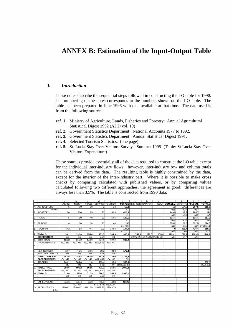
Page 82
ANNEX B: Estimation of the Input-Output Table
I. Introduction
These notes describe the sequential steps followed in constructing the I-O table for 1990.The numbering of the notes corresponds to the numbers shown on the I-O table. Thetable has been prepared in June 1996 with data available at that time. The data used isfrom the following sources: ref. 1. Ministry of Agriculture, Lands, Fisheries and Forestry: Annual Agricultural
Statistical Digest 1992 (ADD vol. 10)ref. 2. Government Statistics Department: National Accounts 1977 to 1992.ref. 3. Government Statistics Department: Annual Statistical Digest 1991.ref. 4. Selected Tourism Statistics. (one page).ref. 5. St. Lucia Stay Over Visitors Survey - Summer 1995 (Table: St Lucia Stay Over
Visitors Expenditure)
These sources provide essentially all of the data required to construct the I-O table exceptfor the individual inter-industry flows; however, inter-industry row and column totalscan be derived from the data. The resulting table is highly constrained by the data,except for the interior of the inter-industry part. Where it is possible to make crosschecks by comparing calculated with published values, or by comparing valuescalculated following two different approaches, the agreement is good: differences arealways less than 3.5%. The table is constructed from 1990 data.
a b c d e f g h i j k l m AGRIC INDUST TRADE SERVICE TOURISM TOTALS HSEHOLD CAP.FOR GOVT DOM.DEM EXPORTS FIN.DEM. TOTALS
A. AGRICULTURE 5 30 10 2 5,3 52,3 73 194,5 267,5 319,8(notes) n1 n18 n15 n14 n7
B. INDUSTRY 20 250 75 30 50,3 425,3 649,5 149,2 798,7 1224n1 n18 n16 n14 n7
C. TRADE 5 20 40 50 67,5 182,5 135,4 0 135,4 317,9n1 n18 n16 n14 n7
D. SERVICE 6 30 30 20 46 132 370,2 22,3 392,5 524,5n1, n10 n18 n16 n14 n7,n9,n13
E. TOURISM 0,2 2,8 0,4 1,3 139,8 144,5 0 415,4 415,4 559,9n1, n11 n18 n8 n14 n12
F. TOTALS 36,2 332,8 155,4 103,3 308,9 936,6 748,3 276,6 170,8 1228,1 781,4 2009,5 2946,1(CORRECTED) n52 n52 n52 n52 n52 ref.2 p.35 ref.2 p.35 2p.35,n19 n19 n17 n20
G. DOM. FINAL 124,8 315,2 143,9 227,1 122,2 932,2FACTOR INPUTS n53, n45 n53, n45 n53, n45 n53, n46 n53, n47
H.
I. NET INDIRECT 18,7 71,6 18,6 30,7 32,8 172,4FINAL FAC. INPUTS n48 n48 n48 n48 n48
J. TOTAL DOM. FIN 143,5 386,8 162,5 257,8 155 1105,6FACTOR INPUTS n54, n49 n54, n49 n54, n49 n54, n49 n54, n49 n56
K. IMPORTS 140,1 504,4 0 163,4 95,6 903,5 902,6n40 n41 n42 n43 n44 (calculated) (ref2,p.35)
L. TOTAL FINAL 283,6 891,2 162,5 421,2 250,6 2009,2FACTOR INPUTS n55, n50 n55, n50 n55, n50 n55, n50 n55, n50
M. TOTALS 319,8 1224 317,9 524,5 559,5 2946,1n51 n51 n51 n51 n51
N. EMPLOYMENT 11666 15174 6720 9958 5603 49121n71, n74 n71,73,74 n71,72,74
O. PRODUCTIVITY 123000,7 25490,97 24181,55 25888,73 27663,75(n74)
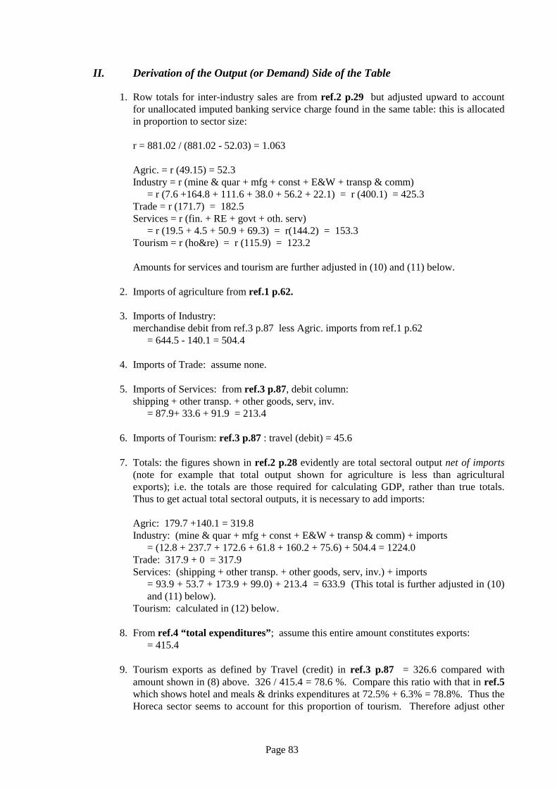
Page 83
II. Derivation of the Output (or Demand) Side of the Table
1. Row totals for inter-industry sales are from ref.2 p.29 but adjusted upward to accountfor unallocated imputed banking service charge found in the same table: this is allocatedin proportion to sector size:
r = 881.02 / (881.02 - 52.03) = 1.063
Agric. = r (49.15) = 52.3Industry = r (mine & quar + mfg + const + E&W + transp & comm)
= r (7.6 +164.8 + 111.6 + 38.0 + 56.2 + 22.1) = r (400.1) = 425.3Trade = r (171.7) = 182.5Services = r (fin. + RE + govt + oth. serv)
= r (19.5 + 4.5 + 50.9 + 69.3) = r(144.2) = 153.3Tourism = r (ho&re) = r (115.9) = 123.2
Amounts for services and tourism are further adjusted in (10) and (11) below.
2. Imports of agriculture from ref.1 p.62.
3. Imports of Industry:merchandise debit from ref.3 p.87 less Agric. imports from ref.1 p.62
= 644.5 - 140.1 = 504.4
4. Imports of Trade: assume none.
5. Imports of Services: from ref.3 p.87, debit column:shipping + other transp. + other goods, serv, inv.
= 87.9+ 33.6 + 91.9 = 213.4
6. Imports of Tourism: ref.3 p.87 : travel (debit) = 45.6
7. Totals: the figures shown in ref.2 p.28 evidently are total sectoral output net of imports(note for example that total output shown for agriculture is less than agriculturalexports); i.e. the totals are those required for calculating GDP, rather than true totals.Thus to get actual total sectoral outputs, it is necessary to add imports:
Agric: 179.7 +140.1 = 319.8Industry: (mine & quar + mfg + const + E&W + transp & comm) + imports
= (12.8 + 237.7 + 172.6 + 61.8 + 160.2 + 75.6) + 504.4 = 1224.0Trade: 317.9 + 0 = 317.9Services: (shipping + other transp. + other goods, serv, inv.) + imports
= 93.9 + 53.7 + 173.9 + 99.0) + 213.4 = 633.9 (This total is further adjusted in (10)and (11) below).
Tourism: calculated in (12) below.
8. From ref.4 “total expenditures”; assume this entire amount constitutes exports:= 415.4
9. Tourism exports as defined by Travel (credit) in ref.3 p.87 = 326.6 compared withamount shown in (8) above. 326 / 415.4 = 78.6 %. Compare this ratio with that in ref.5which shows hotel and meals & drinks expenditures at 72.5% + 6.3% = 78.8%. Thus theHoreca sector seems to account for this proportion of tourism. Therefore adjust other

Page 84
sectors so that in total they lose an amount equal to 21.2% of Tourism exports. For wantof data, assume all of this is reallocated from Total. Output of Services as calculated in(7) above: 633.9 - 0.212 (415.4) = 633.9 - 88.1 = 545.8; this figure is further adjusted in(13) below. The 88.1 reallocated from Services is already included in Tourism exportsas defined in ref.4.
10.Since some of the Services sector is reallocated to Tourism, adjust the inter-industrytotals from (1) accordingly by an amount calculated from the proportional decrease ofservices: (545.8 / 633.9) (153.3) = 132.0
11.Increase the Tourism inter-industry total by the amount transferred from Services:123.2 + (153.3 - 132.0) = 144.5
12.Tourism Total = inter-industry total +exports + 144.5 + 415.4 = 559.9
13 Services Total Output is adjusted downward by the amount of inter-industry salestransferred to tourism in (11): 545.8 - (153.3 - 132.0) = 524.5
14.Sectoral Final Demand (col. l) = sectoral Total Output (col. m) less sectoral total of Inter-industry sales (col. f).
15.Agric. exports from ref.1 p.5.
16.Other exports:Industry: merchandise credit (from ref.3 p.87) less Agric. exports (15).
= 343.7 - 194.5 = 149.2Trade: assume exports = 0.Services: from the credit column of ref.3 p.87, (ship + other transp + other goods, serv,
inv) less transfer to Tourism from (9) above= (0.1 + 35.4 + 74.9) - 88.1 = 22.3
17.CROSS CHECK: the total of the exports column (k) is 781.4 compared with thepublished total in ref.2 p.35 of 778.2, a difference of 0.411%.
18.Domestic demand (col j) = Final Demand (col l) less Exports (col k).
19.CROSS CHECK: compare calculated total domestic demand of 1228.1 with publishedtotals from ref.2 p.35: (households + cap. form. + govt.) = (748.3 + 276.6 + 170.8) =1195.7; the difference is 2.71%
20.CROSS CHECK: Calculate GDP at market prices as total output less total imports (fromref.2 p.35) = 2009.5 - 902.6 = 1106.9; compare with published figure of 1071.3 (ref.2p.35). The difference is 3.32%.
III. Derivation of the Input (or Supply) Side of the Table
Note: • numbers 21 - 39 are not used• results of operations 40 - 52 are shown in the table below
40.Imports of Agric from ref.1 p.62.

Page 85
41.Imports of Industry: merchandise debit (from ref.3 p.87) less Agric imports (40) = 644.5 - 140.1 = 504.4
42.Imports of Trade: assume none.
43.Imports of Services: from ref.3 p.87, debit col., (shipping + oth. transp. + oth. g,s,i) lessreallocation to Tourism = (87.9 + 33.6 + 91.9) - 40 = 173.4. Note that the amount reallocated to Tourism is arbitrary because of lack of data. But thetotal reallocation on the input side carried out in (43) and (46), and implicitly in (48), isapproximately equal to the reallocation on the output side in (9, 10, 11 and 13).
44.Imports of Tourism: travel debit from ref.3 p.87 plus reallocation from services: 45.6 + 40 = 85.6
45.Domestic factor inputs from ref.1 p.5 or ref.2 p.17 and adjusted in proportion to sectorsize to exclude imputed banking service charge by the factor r = 898.92 / (898.92 = 52.0) = 0.9453 Agric: r (130.6) = 123.5 Industry: r (mine & quar + mfg + const + E&W + trnsp & comm.) = r (5.14 + 73.00 + 61.00 + 23.80+ 104.00 + 53.55) = r (320.5) = 303 Trade: r(146.2) = 138.2
46.Domestic factor inputs (Services): (fin + RE + govt + oth serv) from ref.2 p.17 lessreallocation to Tourism (assumed, but see (43)), and then adjusted by r (see (45)): = r ((74.37 + 49.18 + 123.0 + 29.7) - 40) = 223.3
47.Domestic factor inputs (Tourism): Ho & Re. from ref.2 p.17 plus reallocation fromservices, then adjusted by r (see (45): r (77.4 + 40) = 111.0
48.Total net indirect taxes and subsidies from ref.2 p.35 are allocated to sectors inproportion to sectoral Total outputs: r = 172.4 / 2946.1 = .05852
49.Total domestic final factor inputs are calculated as the sum of domestic factor inputs (45,46, 47)and indirect taxes.
50.Total direct inputs are calculated as the sum of total domestic final inputs (49)andimports.
51.Since total sector inputs for each sector must equal total sector outputs, set input totals(row M) equal to output totals (col. m).
52.Inter-industry totals (row F) are calculated as total inputs (row M) less total final factorinputs (row L). But the total of inter-industry purchases thus calculated is 971.2compared with the 936.6 total calculated for inter-industry sales in col. f. Since the inter-industry sales are taken from actual data (with adjustments), the purchases figures shouldbe re-scaled so that total inter-industry purchases are equal to total sales. Thus apply acorrection factor r = (936.6 / 971.2) = 0.9645 to each inter-industry purchase total to getthe final values used in the I - O table. Differences between the preliminary and finalfigures are shown in the corrections row of the table below.

Page 86
53.Add the amounts subtracted from the inter-industry totals (shown in the corrections row)to the domestic final factor inputs, since total sectoral inputs must remain unchanged, andthe original over-estimation of the inter-industry totals must be due to an underestimationof final factor inputs.
54.Recalculate total domestic final factor inputs: row J = row G + row I.
55.Recalculate final factor inputs: row L = row J + row K
56.CROSS CHECK: Total of domestic final factor inputs as calculated here (i.e. includingnet indirect taxes and subsidies)--1105.6--is an estimate of GDP at market prices.Compare with the published figure of 1071.3 from ref.2 p.35. The difference is 3.22%.
IV. Derivation of the Inter-Industry Portion of the Table
Note: • numbers 57-59 are not used.
60.Au goût, as long as row and column totals of the inter-industry portion are respected.
Table 1. Preliminary figures for the supply sectors.
Agric Indus trade Service tour(F) Total inter-industry 37.5 345.0 161.1 107.1 320.5(G) Domestic factor input 123.5 303.0 138.2 223.3 111.0(I) Indirect taxes & sub. 18.7 71.6 18.6 30.7 32.8(J) Total dom. factor inputs 142.2 374.6 156.8 254.0 143.8(K) Imports 140.1 504.4 0 163.4 95.6(L) Total direct inputs 282.3 879.0 156.8 417.4 239.4(M) Total inputs 319.8 1224.0 317.9 524.5 559.5(FF) Corrected values for row (F) 36.2 332.8 155.4 103.3 308.9Corrections for row (F) 1.3 12.2 5.7 3.8 11.2
V. Note on Employment and Productivity
Row J of the input output table shows the total remuneration to domestic factors ofproduction by sector, i.e. total payments (direct and imputed, including all wages,salaries, tips, bonuses, rents, dividends, and undistributed profits) to Labour, Capital, andLand. These earnings may be associated with employment using data from Table 4.8:Employment by Sex by Industry Groupings - 1991 (loose page in papers sent Guyfrom St. Lucia).
71. Combine the sectors into the five used in the I-O table as follows:
Agriculture: 11598Industry: Mining etc. 131
Manufacturing 6751Utilities 575Construction 4960Transport & Comm. 2669

Page 87
15086Trade: 6681Services: Finance 982
Real Estate 948Public Administration 6586Other Services 2562
11081Hotels and Restaurants: 4389
72.Estimate Tourism employment asHoRe / 0.788 (see 9 and 43 in I-O Notes): 4389 / .788 = 5570
73.Re-calculate Services assuming all employment re-allocated toTourism came from this sector: 11081 - (5570 - 4389) = 9900
74.Allocate the 286 sector “not stated” employees in Table 4.8 in proportion to sectoralemployment, and use the domestic factor payments from row J of the I-O table tocalculate productivity per employee:
Table 2. Employment and Productivity
Sector Employment Productivity Per Employee (EC$)Agriculture 11666 12300.70Industry 15174 25490.97Trade 6720 24181.55Services 9958 25888.73Tourism 5603 27663.75

Page 88
ANNEX C: Factors and Weights
This annex contains an overview of the factors and weights that have been used in theoverlay analysis to produce the set of suitability maps used in SIMLUCIA.
4
56789
101112131415161718
19
202122232425262728293031323334353637
38
394041424344454647484950515253
54
5556575859606162636465
A B C D E F G H I J
Factor 1: Land Use Atlasfactor type
Rating per land use function
map: reluse Natural AgricultureIndustry Quarries
Services Trade
TourismRural
residentialUrban
residentialForest
Sea 1 0 0 0 0 0 0 0 0Primary Forest 2 2 2 1 0 0 0 0 10Secondary Forest 3 4 3 2 1 1 1 0 8Scrub Forest 4 6 4 4 1 1 2 1 6Open Woodlands 5 8 6 4 2 2 2 1 4Grasslands 6 6 7 5 3 3 3 2 2Large-Scale Agriculture 7 6 8 5 4 4 4 3 4Intensive Small Farming 8 5 9 6 7 4 7 5 5Mixed Small Farming 9 4 7 5 5 4 6 4 6Rural Settlemant Areas 10 4 6 7 8 6 10 8 4Urban, Commercial, Industrial an 11 2 4 9 10 7 6 10 0
Factor 2: Land Use Actualfactor type
Rating per land use function
map: landuse Natural AgricultureIndustry Quarries
Services Trade
TourismRural
residentialUrban
residentialForest
Natural vegetation 1 10 8 4 4 6 6 6 5Agriculture 2 6 10 6 6 6 8 7 4Industry and Quarries 3 8 5 10 8 4 5 7 2Trade and Services 4 8 3 6 10 7 6 9 2Tourism 5 8 5 6 8 10 4 9 2Rural residential 6 6 8 5 7 5 10 8 4Urban residential 7 6 2 8 9 7 6 10 4Forest 8 5 6 5 4 6 7 5 10Forest reserve 9 2 0 0 0 0 0 0 8Mangrove 10 6 3 0 0 0 3 1 4Sea 11 0 0 0 0 0 0 0 0Beach 12 8 3 4 0 9 0 2 2Coral reef 13 0 0 0 0 0 0 0 0Terminals, ports, airports 14 6 0 9 8 8 2 7 4Infrastructure 15 4 0 2 2 2 3 2 6
Factor 3: Land Tenurefactor type
Rating per land use function
map: reldis Natural AgricultureIndustry Quarries
Services Trade
TourismRural
residentialUrban
residentialForest
Sea 1 0 0 0 0 0 0 0 0Undivided Government 2 4 4 4 4 4 2 2 6Partly Subdivided Government 3 4 6 5 5 5 4 4 6Fully Subdivided Government 4 6 8 6 6 6 6 6 4Para-statal Land 5 6 8 6 6 6 6 6 4Forest Reserve 6 2 0 0 0 0 0 0 8Undivided Private 7 7 8 6 6 6 6 6 3Partly Subdivided Private 8 7 8 8 8 8 8 8 3Fully Subdivided Private 9 8 8 9 9 9 10 10 2Other 10 5 8 8 8 8 9 9 5Settlements 11 8 4 6 6 6 8 10 2
Factor 4: Land Capabilityfactor type
Rating per land use function
map: relcap Natural AgricultureIndustry Quarries
Services Trade
TourismRural
residentialUrban
residentialForest
Sea 1 0 0 0 0 0 0 0 0Suitable Class I 2 1 10 5 6 6 9 9 1Suitable Class II 3 2 8 6 5 5 8 8 2Suitable Class III 4 3 6 7 4 4 7 7 3Suitable Class IV 5 4 5 7 4 4 6 6 4Not Suitable Class V 6 5 4 6 3 3 5 5 5Not Suitable Class VI 7 6 3 6 2 2 4 4 6Not Suitable Class VII 8 8 2 6 1 1 2 2 8Not Suitable Class VIII 9 10 1 5 1 1 1 1 10Settlement 10 8 4 6 6 6 8 10 2

Page 89
68
697071727374757677787980
81
828384858687888990919293
94
9596979899100101102103104
105
106107108109110111112113114115116117118119120
121122123124125126127128129130
A B C D E F G H I J
Factor 5: Life Zonesfactor type
Rating per land use function
map: relzone Natural AgricultureIndustry Quarries
Services Trade
TourismRural
residentialUrban
residentialForest
Sea 1 0 0 0 0 0 0 0 0Tropical dry - very dry forest 2 8 4 8 8 9 4 8 2Tropical dry forest 3 7 6 7 7 8 6 7 3Tropical moist forest 4 6 8 6 6 7 8 6 4Subtropical moist forest 5 5 6 5 5 5 7 5 5Subtropical wet forest 6 4 8 4 4 4 8 4 6Subtropical wet - rain forest 7 2 6 2 2 2 6 2 8Subtropical rain forest 8 0 2 0 0 0 2 0 10Settlement 9 8 4 6 6 6 8 10 2
Factor 6: Rainfallfactor type
Rating per land use function
map: rsurface Natural AgricultureIndustry Quarries
Services Trade
TourismRural
residentialUrban
residentialForest
Sea 1 0 0 0 0 0 0 0 0 < 1520 mm 2 10 4 9 9 9 8 9 11520 - 1778 mm 3 9 6 8 8 8 10 8 31778 - 2032 mm 4 8 8 7 7 7 8 7 52032 - 2286 mm 5 7 9 6 6 6 7 6 62286 - 2540 mm 6 6 6 4 4 4 6 4 72540 - 3045 mm 7 5 4 2 2 2 4 2 83045 - 3810 mm 8 3 2 1 1 1 2 1 9 > 3810 mm 9 1 0 0 0 0 0 0 10
Factor 7: Slopesfactor type
Rating per land use function
map: slopec Natural AgricultureIndustry Quarries
Services Trade
TourismRural
residentialUrban
residentialForest
Sea 1 0 0 0 0 0 0 0 0 < 2.5 % 2 10 10 10 10 10 10 10 22.5 - 5.0 % 3 8 8 6 6 7 7 6 45.0 - 10.0 % 4 6 6 4 4 6 6 4 510.0 - 17.5 % 5 5 4 2 2 4 4 2 617.5 - 25.0 % 6 4 2 1 1 2 2 1 8 > 25.0 % 7 2 0 0 0 0 0 0 10
Factor 8: Land Elevationfactor type
Rating per land use function
map: elevat Natural AgricultureIndustry Quarries
Services Trade
TourismRural
residentialUrban
residentialForest
Sea 1 0 0 0 0 0 0 0 0 < 25 feet 2 10 7 8 10 10 8 8 125 - 50 feet 3 9 8 10 9 9 10 10 250 - 100 feet 4 8 10 9 8 7 9 9 3100 - 200 feet 5 7 9 7 7 6 8 7 4200 - 400 feet 6 6 8 5 5 4 7 5 5400 - 600 feet 7 5 6 3 4 2 6 3 6600 - 800 feet 8 4 4 1 2 1 4 1 7800 - 1000 feet 9 3 2 0 1 0 2 0 81000 - 2000 feet 10 2 0 0 0 0 1 0 9 > 2000 feet 11 1 0 0 0 0 0 0 10
Factor Weights Weight per land use function
Natural AgricultureIndustry Quarries
Services Trade
TourismRural
residentialUrban
residentialForest
N A I S T R U Fw1-land use atlas 1 3 3 1 1 1 2 1 3w2-actual land use 2 3 3 4 3 4 3 4 3w3-land tenure 3 2 2 2 2 2 2 2 2w4-land capability 4 3 4 2 2 2 3 1 3w5-life zones 5 4 3 0 1 1 3 1 4w6-rainfall 6 4 3 0 1 3 3 2 4w7-slopes 7 3 4 3 3 3 4 4 3w8-land elevation 8 2 2 3 3 3 2 3 2
This table is a print-out of the Microsoft Excel Workbook SimLucia.XLS which has twosheets: sheet 1 consists of the table above and features the factors and weights that havebeen applied in the overlay analysis to produce the set of suitability maps used inSIMLUCIA. In the left top corner of sheet 1 you will find a button named ‘MakeLucMac’. If this button is pressed, the Excel macro stored in sheet 2 of the Workbookwill be executed and produce the IDRISI macro named LucMac.IML. If you run thelatter macro in IDRISI, it will generate the set of suitability maps. Thus, with these tools,you can change the factor types and weights and produce your own set of suitabilitymaps

Page 90
ANNEX D: Pointer Shapes
Pointer Shape Description
Standard MS Windows Pointer Shapes
Standard Windows© cursor.
Standard I-beam cursor for editing windows.
Sizing cursor to change the width of the window. Displayed when the pointeris on top of a vertical window border.
Sizing cursor to change the height of the window. Displayed when the pointeris on top of a horizontal window border.
Sizing cursor to change the width and/or the height of the window. Displayedwhen the pointer is on top of a window corner.
Sizing cursor to change the width and/or the height of the window. Displayedwhen the pointer is on top of a window corner.
Context Sensitive pointer to get on-line help on the command you click on.
Specific SIMLUCIA Pointer Shapes
Insert cursor to insert values in an MBB-Dialog edit field by means of the textvalue and table editor.Insert cursor to insert values in an MBB-Dialog edit field by means of thegraph editor.
Insert cursor to insert values in an MBB-Dialog edit field by means of anadditional dialog.
Pen cursor to pick a value from the legend of a map and to enter it in a cell; orto enter ordinal values in the X-Y graph part of the graph editor.Bucket cursor to pick a value from the legend of a map and to enter it in agroup of contiguous cells.