Vrije Universiteit Brussel

Development of an Equivalent Composite Honeycomb ModelSteenackers, G.; Peeters, J.; Ribbens, B.; Vuye, C.

Published in:Applied Composite Materials

DOI:10.1007/s10443-016-9507-2

Publication date:2016

Document Version:Accepted author manuscript

Link to publication

Citation for published version (APA):Steenackers, G., Peeters, J., Ribbens, B., & Vuye, C. (2016). Development of an Equivalent CompositeHoneycomb Model: A Finite Element Study. Applied Composite Materials, 23(6), 1177-1194.https://doi.org/10.1007/s10443-016-9507-2

General rightsCopyright and moral rights for the publications made accessible in the public portal are retained by the authors and/or other copyright ownersand it is a condition of accessing publications that users recognise and abide by the legal requirements associated with these rights.

• Users may download and print one copy of any publication from the public portal for the purpose of private study or research. • You may not further distribute the material or use it for any profit-making activity or commercial gain • You may freely distribute the URL identifying the publication in the public portalTake down policyIf you believe that this document breaches copyright please contact us providing details, and we will remove access to the work immediatelyand investigate your claim.

Download date: 07. Feb. 2022

This item is the archived peer-reviewed author-version of:

Development of an equivalent composite honeycomb model : a finite element study

Reference:Steenackers Gunther, Peeters J., Ribbens B., Vuye Cedric.- Development of an equivalent composite honeycomb model : afinite element studyApplied composite materials - ISSN 0929-189X - 23:6(2016), p. 1177-1194 Full text (Publisher's DOI): http://dx.doi.org/doi:10.1007/S10443-016-9507-2 To cite this reference: http://hdl.handle.net/10067/1342980151162165141

Institutional repository IRUA

Development of an equivalent composite honeycomb model: a finite

element study

G. Steenackersa,b1, J. Peetersa, B. Ribbensa and C. VuyecaUniversity of Antwerp, Op3Mech research group, Salesianenlaan 30, B-2660 Antwerp,

Belgium;bVrije Universiteit Brussel (VUB), Department of Mechanical Engineering (MECH),

Acoustics & Vibration Research Group (AVRG), Pleinlaan 2, B-1050, Brussels, Belgium;cUniversity of Antwerp, EMIB research group, Paardenmarkt 92, B-2000 Antwerp, Belgium

University of Antwerp, Faculty of Applied Engineering, Salesianenlaan 90, 2660 Hoboken

Abstract

Finite element analysis of complex geometries such as honeycomb composites, brings forthseveral difficulties. These problems are expressed primarily as high calculation times but alsomemory issues when solving these models. In order to bypass these issues, the main goal of thisresearch paper is to define an appropriate equivalent model in order to minimize the complexityof the finite element model and thus minimize computation times. A finite element study isconducted on the design and analysis of equivalent layered models, substituting the honeycombcore in sandwich structures. A comparison is made between available equivalent models. Anequivalent model with the right set of material property values is defined and benchmarked,consisting of one continuous layer with orthotropic elastic properties based on different availableapproximate formulas. This way the complex geometry does not need to be created while themodel yields sufficiently accurate results.

Keywords:Composite structures, Finite Element analysis, numerical modeling, lightweight structures

1. Introduction

1.1. Mechanical Properties of Honeycomb Sandwich Panels

Innovation technologies in aircraft design, automotive applications and lightweight con-structions formed the basis for the development of lightweight sandwich panels consisting of ahoneycomb structured layer [1]. Honeycomb structures are often used in composite sandwichpanels. Due to their impact-resistant properties, honeycomb panels are becoming increasinglypopular as shock-absorbing materials combining minimal weight and high bending stiffness [2].

Mainly due to their geometric complexity, it is time consuming and computationally de-manding to create a detailed finite element (FE) model in order to analyze their mechanicalbehaviour. In this paper, the goal is to examine the different approximative formulas based onliterature study and to validate the feasibility of a possible substitute model which can replacethe highly detailed honeycomb structure in a finite element model. This way the FE calculationtime can be seriously reduced.

Preprint submitted to TBD January 6, 2016

A highly detailed honeycomb geometry is used as a benchmark model. In the next step,the equivalent models are generated where the honeycomb sandwich layer will be replacedby a solid material layer with orthotropic material properties. These equivalent models will becompared with the highly detailed FE reference model with respect to accuracy and calculationtimes. The equivalent model that scores best on both parameters can then be used as surrogateorthotropic material layer to replace the honeycomb layer.

Finite element modelling is often applied in honeycomb material analysis and research [3,4, 5, 6, 7], especially when examining the dynamic behaviour of the composite structure. Theidea of carrying out FE simulations on honeycomb panels in order to identify the materialspecifications dates back from the 1980s. Chamis et al. [8], Karlsson en Wetteskog [9], Mar-tinez [10] en Elspass [11, 12] were using NASTRAN models to identify the nine independentelastic property values. Comparable studies are performed by Mistou et al. [13] on aluminumhoneycomb, by Foo et al. [14] on Nomex honeycomb and by Allegri et al. [15] on carbon fibrereinforced honeycomb materials.

The aforementioned studies are always based on ideal, uniform, hexagonal honeycomb cellswithout imperfections, which in reality is often not the case [16]. The way that cell anomaliesare manifesting themselves in the honeycomb structure and respective deviated analysis results,is discused by Hohe en Becker [17]. The influence of irregular cell thickness and geometry onthe mechanical properties is analyzed by Li et al. [18], Yang et al. [19] (cell thickness variation),Simone and Gibson [20, 21] (thickness variations of cell boundaries, cell curvature and crosssection) and finally Guo and Gibson [4] (elimination of cells). In all these papers, a finiteelement model of the honeycomb core layer was used.

1.2. Orthotropic Equivalent Model

The equivalent models are generated by replacing the complex honeycomb geometry by asolid material layer with orthotropic properties. In scientific literature, there is a number ofstudies that try to derive the values of these orthotropic constants. A complete set of 9 elasticconstants for honeycomb layers is difficult to trace in literature as the reference papers mainlyfocus on a partial subset of these constants. Masters en Evans [22] designed a theoreticalmodel to determine E1, E2, ν12 and G12 in two dimensions with the focus on bending and strainmechanisms. They combined the results into a general model that is able to reproduce differentresults.

Qunli Liu [23] developed equivalent formulae for E3, G13 and G23. Abd-el Sayed, Jones andBurgess [24] focused on E1, E2 and ν12 in two dimensions. Grediac [25] and Shi & Tong [26]independently calculated G13 and G23. Both references started from the studies performed byKelsey et al. [27]. Grediac used one quarter of a honeycomb cell as a reference cell and appliedsymmetry rules to simplify the finite element calculations. As a result, the shear modulus iscalculated. Becker [28] formulated E1, E2, ν12, ν32 and G12 by taking into account the thicknessof the honeycomb core. Zhang & Ashby [29] retrieved formulas for E3, ν32, ν13, G13 and G23

in the case of loading perpendicular to the material layer surface. Buckling, delamination andfracture are identified as probability to failure. E. Nast [30] performed a honeycomb layerstudy that is comparable to the work of Abd-el Sayed, Jones en Burgess. Nast applied differentboundary conditions and achieved formulas for the complete set of nine elastic constants. InSection 2 an overview is given of the approximative formulae which will be used further inSection 5 for reduction of computation times.

3

2. Formulae for Orthotropic Elastic Constants

In this section different approximations for the determination of the elastic constants arelisted. The complete list can be found in appendix. The definition of the used symbols arefound in the nomenclature list (Section 7). There are mathematical relationships between thedifferent formulae that yield acceptable approximations. These relationships will be expressedby a K-factor in order to simplify the use of the different approximations with varying geometricparameters. The K-factor will be defined as the ratio of E3 approximated by Liu [23] and E2

approximated by Masters & Evans [22].

Calculation of E3

The following formula for the calculation of E3 is generally accepted and can be found inthe publications of Nast, Liu & Zhang [30, 23, 29]:

E3 =2.E.tc

cosϕ.(1 + sinϕ).a(1)

Calculation of E2

The following formula for the calculation of E2 is developed by Masters & Evans [22]:

E2 =E

1+sinϕcosϕ

.[sin2 ϕ.a3

t3c+ (cos2ϕ).tc

a

] (2)

Dividing Eq. (1) by Eq. (2), yields for K-factor:

K =E3

E2

=

(2.E.tc

cosϕ.(1+sinϕ).a

)(

E

1+sinϕcosϕ

.

[sin2 ϕ.a3

t3c+

(cos2ϕ).tca

]) (3)

After deduction Eq. (4) can be obtained:

K =2.tc

a. cos2 ϕ.(sin2 ϕ.a3

t3c+

cos2 ϕ.tca

)(4)

After rearranging Eq. (5) is obtained

K = 2.(

tan2 ϕ.a2

t2+t2

a2

)(5)

For the common honeycomb geometries, the ratio t2

a2is very small and can be neglected.

With the data from Table 1, a value of t2

a2=1.08E-4 is reached. The K-factor can thus be

reduced to Eq.( 6).

K =2.a2

t2tan2ϕ. (6)

4

3. Determination of Orthotrope Parameter Values for Equivalent Layer

3.1. Definition of Honeycomb Sandwich

The honeycomb structure can be modified based on a set of defined parameters. Themodification of these parameters leads to a change in structural properties of the honeycombsandwich. The most common cell shape within a honeycomb sandwich is the one consistingof uniform hexagonal prism cells. As this cell shape is used most frequently, this one will beexamined although more complex geometrical shapes exist. Figure 1 defines the parameters ofthe honeycomb cell geometry.

a

a/2 α d

tc

2tc

(a) Top view of cell

a

hc

a/2

(b) Front view of cell

Figure 1: Honeycomb geometrical cell parameters

The main objective is to model the sandwich core as a orthotropic material layer. Resultingfrom literature study in Section 1.2 there are different studies carried out to determine theseorthotropic parameter values. In order to determine a set of parameter values that can be usedto model an equivalent sandwich layer in order to bypass time-consuming FE calculations, itis necessary to compare different approximative models. but also benchmark them against adetailed finite element model. As not all studies list formulas for the complete set of parameters,some studies will be combined in order to achieve a complete set of parameters. The parametersneeded for this calculation, are listed in Table 1.

3.2. Finite Element Modeling

research is conducted on the design and analysis of equivalent core models, substituting thehoneycomb core in sandwich structures, in the finite element program Siemens NX 8.0.

5

Table 1: Honeycomb parameters for the definition of the equivalent orthotropic material layer

Item Property ValueCell dimensions tc(mm) 0,0381

a(mm) 3,666α(◦) 120

General dimensions l(mm) 500b(mm) 102,6h(mm) 12,7

Elastic parameters Ew(N/mm2) 69 E+03νw() 0.33Gw(N/mm2) 26 E+03

(a) complex FE model (b) equivalent FE model

Figure 2: higly detailed FE model versus equivalent model

Table 2: Comparison of complex reference model with equivalent model

Item Reference Model ‘CoHC’ Equivalent Model ‘EqO1’Element type Tetra4 Hex8Number of elements 840896 3276Number of nodes 1443907 4480Calculation time [s] 47440 2Memory usage [MB] 4668 100File size [MB] 1610 39

4. Calculation of Equivalent Sandwich Structure

4.1. Introduction

In order to minimize the calculation time of complex FE models, the complex geometryof the honeycomb model is replaced by an equivalent model. In order to achieve this, variousmodels available from literature will be compared. These models will consist of a simple core

6

structure. Different material properties for the core structure will lead to different results andconclusions.

4.2. Orthotrope elastic properties

It is chosen to model the core material with orthotropic material properties. In this paper,it will be useful to combine different formulations in such a way that implementing these valuesin the finite element model yield meaningful output results with respect to the highly-detailedcomposite model. The candidate equivalent models with simplified geometry, as shown inFigure 2(b), are compared with the complex honeycomb model described in Figure 2(a).

It is necessary to compare the different approximations with each other. In Table 3, Table 4and Table 5 the applied parameter values are listed. The geometric properties are listed inTable 1. One can notice that the approximative formula for E1 by Abd El-Sayed [24] results ina value for E1 = 577.6N/mm2 while values resulting from Masters & Evans [22] en Nast [30]are a factor 3500 smaller. As demonstrated in Table 4 it is clear that the values for ν23 en ν13are approaching zero for both applied models.

Table 3: Young’s modulo orthotropic equivalent

Item Model ValueE1(N/mm

2) Masters & Evans [22] 0.179Nast [30] 0.163Abd El-Sayed [24] 577.556

E2(N/mm2) Masters & Evans [22] 0.179

Nast [30] 0.201Abd El-Sayed [24] 509.419

E3(N/mm2) Nast [30] 1103.73

Liu [23] 1103.73Zhang & Ashby [29] 1103.73

Table 4: Poisson’s Ratios orthotropic equivalent

Item Model Valueν12 Masters & Evans [22] 1

Nast [30] 0.752Abd El-Sayed [24] 1

ν23 Nast [30] 6.00 E-05Zhang & Ashby [29] 0

ν13 Nast [30] 7.81 E-05Zhang & Ashby [29] 0

7

Table 5: Shear modulus orthotropic equivalent

Item Model ValueG12(N/mm

2) Masters & Evans [22] 4.47 E-02Nast [30] 4.63 E-02

G13(N/mm2) Grediac [25] 234.01

Nast [30] 416.02Liu [23] 234.01Shi [26] 234.01Zhang & Ashby [29] 234.01

G23(N/mm2) Grediac [25] 156.01

Nast [30] 308.16Liu [23] 156.01Shi [26] 156.01Zhang & Ashby [29] 156.01

From Tables 3, 4 en 5, one can conclude that for the given parameter values, listed in Table 1there is similarity to be detected in the approximations for the orthotropic elastic constants.

Next, the influence of the α-angle on the orthotropic elastic constants is examined. Thisangle mainly defines the hexagonal prism that defines the cell geometry, as shown in Figure 1.

In Fig. 3 the influence of the α-angle on the trend of the Young’s moduli E1 and E2 valuesby Masters [22] and Nast [30] is demonstrated. From Figure 3 one can conclude that the valuesfor the Young’s modulus do not exceed 1N/mm2 for α between 65◦ and 150◦. These valuesare much lower with respect to the calculated values for E3. The approximations of Masters& Evans and Nast voor E2 follow the same evolution but are diverging for E1 at lower anglevalues. This difference is negligible compared to difference found with approximation [24].From this figure, it is thus concluded that for the angle range of α between 105◦ and 150◦ theapproximations for E1 en E2 can be used.

8

0

0,1

0,2

0,3

0,4

0,5

0,6

0,7

0,8

0,9

1

65 75 85 95 105 115 125 135 145

Yo

un

g's

mo

du

lus

(N/m

m²)

α (°)

E2 - Nast

E1 - Masters & Evans

E1 - Nast

E2 - Masters &

Evans

Figure 3: Influence of angle variation on Young’s Modulus values.

5. Modeling the equivalent sandwich layer

A finite element (FE) model is generated that represents the equivalent structure with asandwich layer. The model dimensions (length, width and height) are taken identical to thevalues of the complex FE model. The equivalent model consists of an equivalent core boundedby two sandwich outer plates. The mapped FE mesh is generated with brick elements. Themodel (Figure 4) consists of 3276 elements. A convergence test is carried out to check the meshquality.

Figure 4: Equivalent honeycomb sandwich FE model.

9

In order to define and compare the various equivalent models, a code is defined for eachmodel describing the type of model used during the finite element analysis. The used modelsand respective abbreviations are listed in Table 6 and Table 7.

Table 6: Denomination of different equivalent models

Item DefinitionCoHC model with complex geometryEqIso equivalent model with solid isotropic coreEqOi equivalent model with orthotropic core Oi

Approximative model EqO1 is based on the commonly used orthotropic parameters foundin literature (Table 7). Model EqO2 is defined in order to examine alternative models andvalues for E1 and E2 with respect to approximative model EqO1. Other used models andvalues for G13 and G23 with respect to EqO1 are examined by the definition of model EqO3.The influence of v12 is examined in equivalent model EqO4. Table 7 gives an overview of thedefined approximations for each of the nine elastic constants used in the four approximativeequivalent models for the core composite layer.

Table 7: Definition orthotropic core

Property Model O1 Model O2 Model O3 Model O4E1 Masters [22] Abd El-Sayed [24] Masters [22] Masters [22]E2 Nast [30] Abd El-Sayed [24] Nast [30] Masters [22]E3 Nast [30] Liu [23] Nast [30] Liu [23]v12 Masters [22] Masters [22] Masters [22] Nast [30]v23 Zhang [29] Zhang [29] Zhang [29] Zhang [29]v13 Zhang [29] Zhang [29] Zhang [29] Zhang [29]G12 Masters [22] Masters [22] Masters [22] Masters [22]G13 Liu [23] Liu [23] Nast [30] Grediac [25]G23 Grediac [25] Grediac [25] Nast [30] Liu [23]

6. Discussion of Results

6.1. Loading Conditions

In this section the different analysis results will be compared and discussed. The equiv-alent models are subjected to a number of loading cases, listed in Table 8. Also the modalanalysis results are used to compare the different models. The performance of the differentapproximations is compared with the highly detailed finite element model results.

These loading conditions are given a specific name depending on the direction of the appliedload. For example, a clamped sandwich structure in the B-H plane and subject to an appliedload in the L-direction, is defined as ‘B,H,L’ (Figure 5). This leads to a large number of possible

10

Table 8: Applied set of five loading conditions.

Item Constraining Direction ~F F(N)B,H,H B,H-face H 250B,L,L B,L-face L 250B,L,H B,L-face H 250B,L,B B,L-face B 250H,L,H L,H-face H 250

Figure 5: Definition of loading condition ‘B,H,L’.

loading cases of which five were selected for comparison, as shown in Table 8. Not all loadingcases are equally important because in some cases the honeycomb layer has little or no effecton the bending stiffness of the composite structure [31]. As a consequence, the remaining loadcases to be used are listed in Table 8. In addition to the applied loading conditions, listed inTable 8, also a modal analysis is applied in order to compare the different equivalent models.The first four eigenfrequencies are analyzed and compared.

6.2. Static Deflections and Eigenfrequencies

The results for the 5 load cases are listed in Tables 9 and 10. Table 11 lists the results fromthe modal analysis.

Table 9: Calculated deflections for five applied load cases

Load Case CoHc [mm] EqO1 [mm] ∆1 [%] EqO2 [mm] ∆2 [%] EqO3 [mm] ∆3 [%] EqO4 [mm] ∆4 [%]BHH 4.1 4.26 3.90 4.2 2.44 4.14 0.98 4.26 3.90BLL 2.55E-04 2.71E-04 6.27 7.74E-04 203.53 1.52E-04 40.39 2.79E-04 9.41BLH 5.45E-05 5.88E-05 7.89 5.89E-05 8.07 5.90E-05 8.26 5.88E-05 7.89BLB 4.20E-04 4.31E-04 2.62 4.38E-04 4.29 2.27E-04 45.95 4.20E-04 0.00HLH 2.11E-02 2.04E-02 3.32 2.04E-02 3.32 1.36E-02 35.55 2.04E-02 3.32Mean [%] 4.80 44.33 26.22 4.90

11

Table 10: Calculated deflections for 5 applied load cases in mm (cont’d)

Load Case CoHc [mm] EqIso [mm] ∆iso [%]BHH 4.1 4.22 2.93BLL 2.55E-04 1.54E-04 39.61BLH 5.45E-05 4.00E-05 26.61BLB 4.20E-04 1.66E-04 60.48HLH 2.11E-02 1.17E-02 44.55Mean [%] 34.83

From Table 9 one can conclude that the approximative model that yields overall the mostaccurate results with respect to the deflection values, is model ‘EqO1’ (mean difference of 4.8%),closely followed by model ‘EqO4’ (4.9% mean difference). The main difference is situated inloading condition BLL where model ‘EqO4’ is less accurate with a relative error of 9.4%.The least accurate approximative model with respect to deflection values, is model ‘EqO2’yielding a mean difference of 44.3%. This is mainly due to the noticeable difference for loadingcondition BLL. When not taking into account this loading condition, model ‘EqO2’ yieldsa mean relative difference of 4.5% which has the same order of magnitude as model ‘EqO1’(4.4%) and model ‘EqO4’ (3.8%). When looking at the deflection magnitude for the isotropicmodel ‘EqIso’ one can conclude that this model is the least accurate model with the highestrelative difference for loading conditions BLH, BLB and HLH. One can thus conclude that thismodel is not acceptable as an approximative FE model for honeycomb composites.

Table 11: Calculated eigenfrequencies for five applied load cases

CoHc [Hz] EqIso [Hz] ∆ [%] EqO1 [Hz] ∆ [%] EqO2 [Hz] ∆ [%] EqO3 [Hz] ∆ [%] EqO4 [Hz] ∆ [%]496.30 518.9 4.55 493.10 0.64 495.4 0.18 517.4 4.25 493.1 0.64843.20 994 17.90 834.70 1.01 835 0.98 991 17.58 835 1.011095.00 1220 11.60 1080.00 1.37 1080 1.19 1220 11.42 1080 1.371619.00 1840 13.47 1609.00 0.62 1610 0.56 1810 11.55 1610 0.62Mean [%] 11.88 0.91 0.73 11.20 0.91

From Table 11 one can conclude that the approximative model that yields the most accurateoverall results with respect to the eigenfrequencies values, is model ‘EqO2’ (mean difference of0.7%), closely followed by model ‘EqO4’ (0.9% mean difference) but also model ‘EqO1’ (0.9%mean difference). Model ‘EqO2’ scores best on all 4 eigenfrequencies and the difference withrespect to ‘EqO1’ and ‘EqO4’ is mainly due to eigenfrequency 1 which is the frequency of thefirst bending mode. The least accurate model is again model ‘EqIso’ with a mean differenceof 11.9%. One can thus conclude that an isotropic equivalent model is does not yield accurateresults and is not to be chosen as equivalent model to replace the honeycomb layer. Thus it isnecessary to use an equivalent orthotropic material layer.

12

Figure 6: Deflections of models CoHC, EqO1 and EqO2 for load case BHH.

When looking for an overall most suitable accurate model, one can notice that ‘EqO1’and model ‘EqO4’ only slightly differ with respect to average relative differences. The reasonthat model ‘EqO2’ does not score on the same level as ‘EqO4’, is only due to the differencewith respect to deflection from loading condition BLL. From these results it is clear thatmodel ‘EqO3’ shows important differences for loading cases BLL, BLB en HLH. Once can thusconclude that the approximative model developed by E. Nast [30] for G13 en G23 insufficientlyapproximates the complex model.

Despite the fact that the approximations for E1 and E2 show strong differences betweeneach other (model ‘EqO1’ and ‘EqO2’ only differentiate in the approximation for E1 and E2),there is no significant difference, nor on the level of eigenfrequencies neither on the level ofdisplacement amplitudes. One can conclude from the results that models ‘EqO1’ and ‘EqO2’yield very close results with respect to each other. Figure 6 visualizes the three fine modelsin 400 nodes along the principal direction of the sandwich beam. It is clear that the twoequivalent models approximate the fine honeycomb model accurately. Once can conclude fromthe simulation results that the deflections values but also eigenfrequencies do not deviate morethan 4% with ‘EqO1’ and ‘EqO2’.

6.3. Stress Analysis of an Equivalent Material Layer

In Figure 7 the stress distribution of load case BHH is displayed. One can notice that theouter layers reach a maximum stress value of 22MPa. This stress magnitude is also presentin the equivalent models, as visualized in Figure 8 for model ‘EqO1’. Based on this result,onecan conclude that the equivalent models yield stress values that closely match these of thehighly-detailed model.

13

Figure 7: Stress outline model ‘CoHc’ with BHH loading.

Figure 8: Stress outline equivalent model ‘EqO1’ with BHH loading.

The largest benefit of using the equivalent model is shown in Table 2, where the complexityand computational effort (time and storage) of the two models are compared. The values arelisted for the modal analysis calculations presented in Table 11. When comparing these results,one can notice that the calculation time is reduced with an order of magnitude 105. This is alsonoticeable in the necessary file size of the saved calculation results. A reduction of the number ofnodes with a factor 322 is also achieved. It is noteworthy that even a model with 12 honeycombcells needs a considerable calculate time of 13 hours. In reality, honeycomb sandwich modelswith more than 10000 cells are common, resulting in even higher computation times. By makinguse of equivalent models containing optimized orthotropic material parameter values resultingfrom approximate formulas, these high computation times can be eliminated without strayingtoo far from the exact solutions.

7. Conclusion

From running simulations, it is easy to state that finite element models containing hon-eycomb sandwich layers are yielding high computation times. The main goal of this research

14

paper is to define an appropriate equivalent model in order to minimize the complexity of thefinite element model and thus minimize FE calculation time. In order to minimize these com-putation times, but also the time to create a highly detailed honeycomb sandwich layer, anequivalent model with the right set of material property values is defined based on literaturestudy on the available models. The most accurate equivalent model consists of one continu-ous layer with orthotropic elastic constants and calculated values based on different availableapproximate formulas. This way the complex geometry does not need to be created while themodel yields sufficiently accurate results.

When comparing these results, one can notice that the calculation time is reduced withorder of magnitude 105. This is also noticeable in the necessary file size of the saved calculationresults. A reduction of the number of nodes with a factor 322 is also achieved. This is the mostimportant results of this research, in order to minimize FE calculation times as the complexFE honeycomb models needs 13h to calculate the output results. It is noteworthy that even amodel with 12 honeycomb cells needs this huge calculate time. In reality, honeycomb sandwichmodels with more than 10000 cells are common, resulting in even higher computation times. Bymaking use of equivalent models containing optimized orthotropic material parameter valuesresulting from approximate formulas, these high computation times can be eliminated.

Acknowledgements

This research has been funded by the University of Antwerp and the Institute for thePromotion of Innovation by Science and Technology in Flanders (IWT) by the support to theTETRA project ’Smart data clouds’ with project number 140336. Furthermore, the researchleading to these results has received funding from Industrial Research Fund FWO Krediet aannavorsers 1.5.240.13N. The authors also acknowledge the Flemish government (GOA-Optimech)and the research councils of the Vrije Universiteit Brussel (OZR) and University of Antwerp(fti-OZC) for their funding.

15

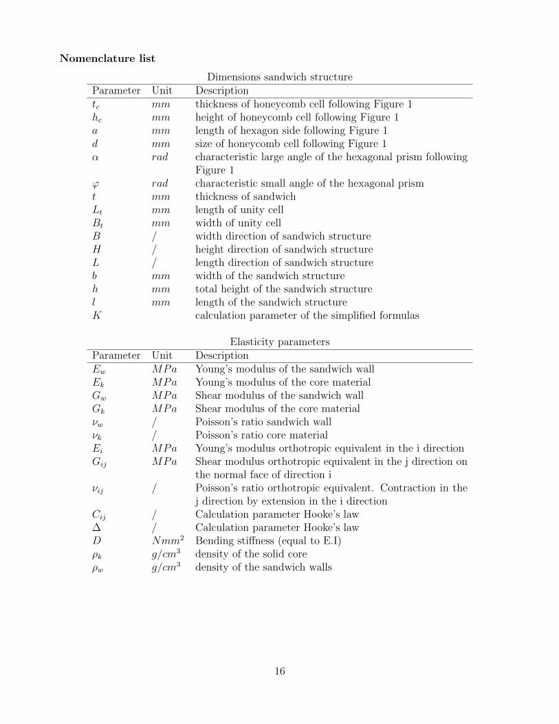
Nomenclature list

Dimensions sandwich structureParameter Unit Descriptiontc mm thickness of honeycomb cell following Figure 1hc mm height of honeycomb cell following Figure 1a mm length of hexagon side following Figure 1d mm size of honeycomb cell following Figure 1α rad characteristic large angle of the hexagonal prism following

Figure 1ϕ rad characteristic small angle of the hexagonal prismt mm thickness of sandwichLt mm length of unity cellBt mm width of unity cellB / width direction of sandwich structureH / height direction of sandwich structureL / length direction of sandwich structureb mm width of the sandwich structureh mm total height of the sandwich structurel mm length of the sandwich structureK calculation parameter of the simplified formulas

Elasticity parametersParameter Unit DescriptionEw MPa Young’s modulus of the sandwich wallEk MPa Young’s modulus of the core materialGw MPa Shear modulus of the sandwich wallGk MPa Shear modulus of the core materialνw / Poisson’s ratio sandwich wallνk / Poisson’s ratio core materialEi MPa Young’s modulus orthotropic equivalent in the i directionGij MPa Shear modulus orthotropic equivalent in the j direction on

the normal face of direction iνij / Poisson’s ratio orthotropic equivalent. Contraction in the

j direction by extension in the i directionCij / Calculation parameter Hooke’s law∆ / Calculation parameter Hooke’s lawD Nmm2 Bending stiffness (equal to E.I)ρk g/cm3 density of the solid coreρw g/cm3 density of the sandwich walls

16

Addendum: Orthotropic elastic constants

All in literature described different approaches of the determination of the nine orthotropicelastic constants are tabulated in this addendum. The definition of the used coordinate systemreference is shown in Figure 9. The explanation of the used symbols is found in the nomenclaturelist.

Figure 9: Reference system

Calculation E1

Masters & Evans [22]

E1 =E

cosϕ1+sinϕ

.[cos2 ϕ.a3

t3c+ (2+sin2 ϕ).tc

a

] (7)

Nast [30]

E1 =t3c .(1 + sinϕ).E

12a3. cos2 ϕ.[1−cosϕ

8+ cosϕ

12

].(1 − ν2)

(8)

Abd El-Sayed [24]

E1 =6.cosϕ. tan2 ϕ.tc.E[a2

4. tan2 ϕ.h2c

+ sinϕ+ a. cosϕ2

].a

(9)

Calculation E2

Masters & Evans [22]

E2 =E

1+sinϕcosϕ

.[sin2 ϕ.a3

t3c+ (cos2ϕ).tc

a

] (10)

17

Nast [30]

E2 =E.t3c . cosϕ

(1 + sinϕ).a3. sin2 ϕ.(1 − ν2)(11)

Abd El-Sayed [24]

E2 =2.E.tc. cosϕ

3.[

a2

4. tan2 ϕ.h2c

+ cos2 ϕ].a

(12)

Calculation E3

Universally accepted(Nast, Liu, Zhang)[30, 23, 29]

E3 =2.E.tc

cosϕ.(1 + sinϕ).a(13)

Calculation G12

Masters & Evans [22]

G12 =E

3. cosϕ.a3

(1+sinϕ).t3c+[

cosϕ+ a. tanϕ.(1 + sinϕ)]. atc

(14)

Nast [30]

G12 =E.t3c .(sinϕ+ 1)

a3.(1 − ν2). cosϕ.(6, 25 − 6. sinϕ)(15)

Calculation G23

Liu, Grediac, Zhang [23, 25, 29]

G23 =cosϕ.tc.G

(1 + sinϕ).a(16)

Nast [30]

G23 =10.tc.G

9.(1 + sinϕ).a. cosϕ3(17)

Shi [26]

G23 =tanϕ.tc.G

a(18)

Calculation G13

Liu [23]

G13 =(1 + sinϕ).G.tc

2. cosϕ.a(19)

Nast [30]

G13 =2.G.tc

cosϕ.a(1 + sinϕ)(20)

Shi [26]

G13 =3.G.tc. tanϕ

2.a(21)

18

Grediac, Ashby [25, 29]

G13 <(1 + sin2 ϕ).G.tc

(1 + sinϕ). cosϕ.a(22)

G13 >(1 + sinϕ).G.tc

2. cosϕ.a(23)

Calculation ν12

Masters & Evans [22]

ν12 =(1 + sinϕ). sinϕ

cos2 ϕ(24)

Nast [30]

ν12 =(1 + sinϕ). sin2 ϕ

12. cos2 ϕ.[cosϕ3

− 1+cosϕ8

] (25)

Abd El-Sayed [24]ν12 = 3. tan2 ϕ (26)

Calculation ν23

Nast [30]

ν23 =t2c . cos2 ϕ.ν

2.a2. sin2 ϕ.(1 − ν2)(27)

Calculation ν13

Nast [30]

ν13 =t2c .(1 + sinϕ)2.ν

24.a2. cosϕ.[cosϕ3

− 1+cosϕ8

].(1 − ν2)

(28)

References

[1] J. Kee Paik, A. K. Thayamballi, G. Sung Kim, The strength characteristics of alu-minum honeycomb sandwich panels, ThinWalled Structures 35 (3) (1999) 205–231.doi:10.1016/S0263-8231(99)00026-9.URL http://linkinghub.elsevier.com/retrieve/pii/S0263823199000269

[2] A. Abbadi, Y. Koutsawa, A. Carmasol, S. Belouettar, Z. Azari, Experimental and nu-merical characterization of honeycomb sandwich composite panels, Simulation ModellingPractice and Theory 17 (10) (2009) 1533–1547. doi:10.1016/j.simpat.2009.05.008.URL http://linkinghub.elsevier.com/retrieve/pii/S1569190X09000604

[3] S. D. Papka, S. Kyriakides, Experiments and full-scale numerical simulations of in-planecrushing of a honeycomb, Acta Materialia 46 (8) (1998) 2765–2776. doi:10.1016/S1359-6454(97)00453-9.URL http://linkinghub.elsevier.com/retrieve/pii/S1359645497004539

19

[4] X. E. Guo, L. J. Gibson, Behavior of Intact and Damaged Honeycombs: a Finite ElementStudy, International Journal of Mechanical Sciences 41 (1) (1999) 85–105.

[5] D. Ruan, G. Lu, B. Wang, T. X. Yu, In-plane dynamic crushing of honeycombsa fi-nite element study, International Journal of Impact Engineering 28 (2) (2002) 161–182.doi:10.1016/S0734-743X(02)00056-8.URL http://linkinghub.elsevier.com/retrieve/pii/S0734743X02000568

[6] Z. Zou, Reid, P. Tan, S. Li, J. Harrigan, Dynamic crushing of honeycombs and features ofshock fronts, International Journal of Impact Engineering 36 (1) (2009) 165–176.URL http://discovery.ucl.ac.uk/170690/

[7] Z. Zheng, J. Yu, J. Li, Dynamic crushing of 2D cellular structures: A finite el-ement study, International Journal of Impact Engineering 32 (1-4) (2005) 650–664.doi:10.1016/j.ijimpeng.2005.05.007.URL http://linkinghub.elsevier.com/retrieve/pii/S0734743X05000795

[8] C. C. Chamis, R. A. Aiello, P. L. N. Murthy, Apparent properties of a honeycomb coresandwich panel by numerical experiments, Journal of Composites Technology and Research10 (1988) 93–99.

[9] U. Karlsson, N. Wetteskog, Ekvivalenta Styvhetsparametrar for Honeycomb, Master’s the-sis, Chalmers Tekisnka Hogskola, Zweden (1987).

[10] R. M. Martinez, Apparent properties of a honeycomb core sandwich panel by numericalexperiment, Master’s thesis, University of Texas (1989).

[11] W. Elspass, Thermostabile Strukturen in Sandwichbauweise, Ph. d. thesis, EidgenossischeTechnische Hochschule Zurich, Switzerland (1989).

[12] W. Elspass, Design of High Precision Sandwich Structures Using Analytical and FiniteElement Models, in: 6th World Congress on Finite Element Methods, Banff, Canada,1990, pp. 658–664.

[13] S. Mistou, M. Sabarots, M. Karama, Experimental and numerical simulations of the staticand dynamic behaviour of sandwich plates, in: European Congress on ComputationalMethods in Applied Sciences and Engineering, Barcelona, Spanje, 2000.

[14] C. C. Foo, G. B. Chai, L. K. Seah, A model to predict low-velocity impact response anddamage in sandwich composites, Composites Science and Technology 68 (6) (2008) 1348–1356. doi:10.1016/j.compscitech.2007.12.007.URL http://www.sciencedirect.com/science/article/pii/S0266353807004757

[15] G. Allegri, U. Lecci, M. Machetti, F. Poscente, FEM Simulation of the Mechanical Be-haviour of Sandwich Materials for Aerospace Structures, Key Engineering Materials 221-222 (2002) 209–220.

[16] L. Gornet, S. Marguet, G. Marckmann, Failure and Effective Elastic Properties Predictionsof Nomex Honeycomb Cores, in: 12th European Conference on Composite Materials,Biarritz, Frankrijk, 2006.

20

[17] J. Hohe, W. Becker, Effective stress-strain relations for two-dimensional cellular sand-wich cores: Homogenization, material models, and properties, Applied Mechanics Reviews55 (1) (2002) 61. doi:10.1115/1.1425394.URL http://link.aip.org/link/AMREAD/v55/i1/p61/s1&Agg=doi

[18] K. Li, X. L. Gao, J. Wang, Dynamic crushing behavior of honeycomb structures withirregular cell shapes and non-uniform cell wall thickness, International Journal of Solidsand Structures 44 (14-15) (2007) 5003–5026. doi:10.1016/j.ijsolstr.2006.12.017.URL http://linkinghub.elsevier.com/retrieve/pii/S0020768306005427

[19] M.-Y. Yang, J.-S. Huang, J. W. Hu, Elastic Buckling of Hexagonal Honeycombs with DualImperfections, Composite Structures 82 (3) (2008) 326–335.

[20] A. E. Simone, L. J. Gibson, Effects of solid distribution on the stiffness and strength ofmetallic foams, Acta Materialia 46 (6) (1998) 2139. doi:10.1016/S1359-6454(97)00421-7.URL http://linkinghub.elsevier.com/retrieve/pii/S1359645497004217

[21] A. E. Simone, L. J. Gibson, The effects of cell face curvature and corrugations onthe stiffness and strength of metallic foams, Acta Materialia 46 (11) (1998) 3929–3935.doi:10.1016/S1359-6454(98)00072-X.URL http://linkinghub.elsevier.com/retrieve/pii/S135964549800072X

[22] I. G. Masters, K. E. Evans, Models for the elastic deformation of honeycombs, CompositeStructures 35 (4) (1996) 403–422. doi:10.1016/S0263-8223(96)00054-2.URL http://linkinghub.elsevier.com/retrieve/pii/S0263822396000542

[23] Q. Liu, Y. Zhao, Effect of Soft Honeycomb Core on Flexural Vibration of Sandwich Panelusing Low Order and High Order Shear Deformation Models, Journal of Sandwich Struc-tures and Materials 9 (2007) 95–108.

[24] F. K. A. El-Sayed, R. Jones, I. W. Burgess, A theoretical approach to the defor-mation of honeycomb based composite materials, Composites 10 (4) (1979) 209–214.doi:10.1016/0010-4361(79)90021-1.URL http://www.sciencedirect.com/science/article/pii/0010436179900211

[25] M. Grediac, A finite element study of the transverse shear in honeycomb cores, Inter-national Journal of Solids and Structures 30 (13) (1993) 1777–1788. doi:10.1016/0020-7683(93)90233-W.URL http://linkinghub.elsevier.com/retrieve/pii/002076839390233W

[26] G. Shi, P. Tong, Equivalent transverse shear stiffness of honeycomb cores, Interna-tional Journal of Solids and Structures 32 (10) (1995) 1383–1393. doi:10.1016/0020-7683(94)00202-8.URL http://linkinghub.elsevier.com/retrieve/pii/0020768394002028

[27] S. Kelsey, R. A. Gellatly, B. W. Clark, The Shear Modulus of Foil HoneycombCores: A Theoretical and Experimental Investigation on Cores Used in SandwichConstruction, Aircraft Engineering and Aerospace Technology 30 (10) (1958) 294–302.

21

doi:10.1108/eb033026.URL http://www.emeraldinsight.com/10.1108/eb033026

[28] W. Becker, Closed-form analysis of the thickness effect of regular honeycomb core material,Composite Structures 48 (1-3) (2000) 67–70. doi:10.1016/S0263-8223(99)00074-4.URL http://linkinghub.elsevier.com/retrieve/pii/S0263822399000744

[29] J. Zhang, M. F. Ashby, The out-of-plane properties of honeycombs, International Journalof Mechanical Sciences 34 (6) (1992) 475–489. doi:10.1016/0020-7403(92)90013-7.URL http://linkinghub.elsevier.com/retrieve/pii/0020740392900137

[30] E. Nast, On honeycomb-type core moduli, in: 38th Structures, Structural Dynam-ics, and Materials Conference, Structures, Structural Dynamics, and Materials andCo-located Conferences, American Institute of Aeronautics and Astronautics, 1997.doi:doi:10.2514/6.1997-1178.URL http://dx.doi.org/10.2514/6.1997-1178

[31] T. Legon, The equivalent modeling and analysis of aluminum honeycomb structures, afinite element study, Master’s thesis, Artesis University College (2013).

22