Vrije Universiteit, Amsterdam Faculty of Sciences ... › ~boncz › msc › 2014-Barca.pdf ·...
113
Vrije Universiteit, Amsterdam Faculty of Sciences, Computer Science Department Cristian Mihai Bârcă, student no. 2514228 Dynamic Resource Management in Vectorwise on Hadoop Master Thesis in Parallel and Distributed Computer Systems Supervisor / First reader: Prof. Dr. Peter Boncz, Vrije Universiteit, Centrum Wiskunde & Informatica Second reader: Prof. Dr. Henri Bal, Vrije Universiteit Amsterdam, August 2014
Transcript of Vrije Universiteit, Amsterdam Faculty of Sciences ... › ~boncz › msc › 2014-Barca.pdf ·...

Vrije Universiteit, Amsterdam
Faculty of Sciences,Computer Science Department
Cristian Mihai Bârcă, student no. 2514228
Dynamic Resource Management inVectorwise on Hadoop
Master Thesis in Parallel and DistributedComputer Systems
Supervisor / First reader:Prof. Dr. Peter Boncz, Vrije Universiteit, Centrum Wiskunde & Informatica
Second reader:Prof. Dr. Henri Bal, Vrije Universiteit
Amsterdam, August 2014

Contents
1 Introduction 11.1 Background and Motivation . . . . . . . . . . . . . . . . . . . . . . . . . . . . . . 11.2 Related Work . . . . . . . . . . . . . . . . . . . . . . . . . . . . . . . . . . . . . . 2
1.2.1 Hadoop-enabled MPP Databases . . . . . . . . . . . . . . . . . . . . . . . 41.2.2 Resource Management in MPP Databases . . . . . . . . . . . . . . . . . . 71.2.3 Resource Management in Hadoop Map-Reduce . . . . . . . . . . . . . . . 81.2.4 YARN Resource Manager (Hadoop NextGen) . . . . . . . . . . . . . . . . 9
1.3 Vectorwise . . . . . . . . . . . . . . . . . . . . . . . . . . . . . . . . . . . . . . . . 111.3.1 Ingres-Vectorwise Architecture . . . . . . . . . . . . . . . . . . . . . . . . 121.3.2 Distributed Vectorwise Architecture . . . . . . . . . . . . . . . . . . . . . 131.3.3 Hadoop-enabled Architecture . . . . . . . . . . . . . . . . . . . . . . . . . 16
1.4 Research Questions . . . . . . . . . . . . . . . . . . . . . . . . . . . . . . . . . . . 191.5 Goals . . . . . . . . . . . . . . . . . . . . . . . . . . . . . . . . . . . . . . . . . . 201.6 Basic ideas . . . . . . . . . . . . . . . . . . . . . . . . . . . . . . . . . . . . . . . 20
2 Approach 212.1 HDFS Local Reads: DataTransferProtocol vs Direct I/O. . . . . . . . . . . . . . 222.2 Towards Data Locality . . . . . . . . . . . . . . . . . . . . . . . . . . . . . . . . . 242.3 Dynamic Resource Management . . . . . . . . . . . . . . . . . . . . . . . . . . . 262.4 YARN Integration . . . . . . . . . . . . . . . . . . . . . . . . . . . . . . . . . . . 282.5 Experimentation Platform . . . . . . . . . . . . . . . . . . . . . . . . . . . . . . . 31
3 Instrumenting HDFS Block Replication 333.1 Preliminaries . . . . . . . . . . . . . . . . . . . . . . . . . . . . . . . . . . . . . . 333.2 Custom HDFS Block Placement Implementation . . . . . . . . . . . . . . . . . . 35
3.2.1 Adding (New) Metadata to Database Locations . . . . . . . . . . . . . . . 363.2.2 Extending the Default Policy . . . . . . . . . . . . . . . . . . . . . . . . . 36
4 Dynamic Resource Management 424.1 Worker-set Selection . . . . . . . . . . . . . . . . . . . . . . . . . . . . . . . . . . 424.2 Responsibility Assignment . . . . . . . . . . . . . . . . . . . . . . . . . . . . . . . 474.3 Dynamic Resource Scheduling . . . . . . . . . . . . . . . . . . . . . . . . . . . . . 53
5 YARN integration 675.1 Overview: model resource requests as separate YARN applications . . . . . . . . 685.2 DbAgent–Vectorwise communication protocol:
update worker-set state, increase/decrease resources . . . . . . . . . . . . . . . . 725.3 Workload monitor & resource allocation . . . . . . . . . . . . . . . . . . . . . . . 73
6 Evaluation & Results 806.1 Evaluation Plan . . . . . . . . . . . . . . . . . . . . . . . . . . . . . . . . . . . . . 806.2 Results Discussion . . . . . . . . . . . . . . . . . . . . . . . . . . . . . . . . . . . 83
i

List of Figures
1.1 Hadoop transition from v1 to v2 . . . . . . . . . . . . . . . . . . . . . . . . . . . 101.2 The Ingres-Vectorwise (single-node) High-level Architecture . . . . . . . . . . . . 121.3 The Distributed Vectorwise High-level Architecture . . . . . . . . . . . . . . . . . 141.4 The Vectorwise on Hadoop High-level Architecture (the session-master, or Vec-
torwise Master, is involved in query execution). . . . . . . . . . . . . . . . . . . . 17
2.1 The Vectorwise on Hadoop dynamic resource management approach in 7 steps. . 222.2 Local reads through DataNode (DataTransferProtocol). . . . . . . . . . . . . . . 232.3 Direct local reads (Direct I/O - open(), read() operations). . . . . . . . . . . . . 232.4 A flow network example for the min-cost problem, edges are annotated with
(cost, flow / capacity). . . . . . . . . . . . . . . . . . . . . . . . . . . . . . . . . . 272.5 The flow network (bipartite graph) model used to determine the responsibility
assignment. . . . . . . . . . . . . . . . . . . . . . . . . . . . . . . . . . . . . . . . 282.6 Out-of-band approach for Vectorwise-YARN integration. . . . . . . . . . . . . . . 30
3.1 An example of two tables (R and S) loaded on 3 workers / 4 nodes, using 3-waypartitioning and replication degree of 2: after the initial-load (upper image) vs.during a system failover (lower image). . . . . . . . . . . . . . . . . . . . . . . . . 34
3.2 Instrumenting the HDFS block replication, in three scenarios, to maintain block(co-)locality to worker nodes. . . . . . . . . . . . . . . . . . . . . . . . . . . . . . 35
3.3 Baseline (default policy) vs. collocation (custom policy) – HDFS I/O throughputmeasured in 3 situations (1) healty state, (2) failure state (2 nodes down), (3)recovered state. Queries 1, 4, 6, and 12 on partitioned tables, 32-partitioning, 8workers / 10 Hadoop "Rocks" nodes, 32 mpl. . . . . . . . . . . . . . . . . . . . . 40
4.1 Starting the Vectorwise on Hadoop worker-set through VectorwiseLauncher andDbAgent. All related concepts to this section are emphasized with a bold blackcolor. . . . . . . . . . . . . . . . . . . . . . . . . . . . . . . . . . . . . . . . . . . . 43
4.2 The flow network (bipartite graph) model used to match partitions to workernodes. . . . . . . . . . . . . . . . . . . . . . . . . . . . . . . . . . . . . . . . . . . 46
4.3 Assigning responsibilities to worker nodes. All related concepts to this sectionare emphasized with bold black and red/blue/green colors (for single (partition)responsibilities). . . . . . . . . . . . . . . . . . . . . . . . . . . . . . . . . . . . . 48
4.4 The flow network (bipartite graph) model used to assign responsibilities to work-ers nodes. . . . . . . . . . . . . . . . . . . . . . . . . . . . . . . . . . . . . . . . . 49
4.5 The flow network (bipartite graph) model used to calculate a part of the resourcefootprint (what nodes and table partitions we use for a query, given the worker’savailable resource and data-locality). Note: fx is the unit with which we increasethe flow along the path at step x of the algorithm. . . . . . . . . . . . . . . . . . 57
ii

LIST OF FIGURES iii
4.6 Selecting the (partition responsibilities and worker nodes involved in query ex-ecution. Only the first two workers from left are chosen (bold-italic black) fortable scans; first one reads from two partitions (red and green), whereas thesecond reads just from one (blue). The third worker is considered overloadedand so, it is excluded from the I/O. Red/blue/green colors are used to expressmultiple (partition) responsibilities. . . . . . . . . . . . . . . . . . . . . . . . . . . 58
5.1 Timeline of different query workloads. . . . . . . . . . . . . . . . . . . . . . . . . 695.2 Out-of-band approach for Vectorwise-YARN integration. An example using 2 x
Hadoop nodes that equally share 4 x YARN containers. . . . . . . . . . . . . . . 705.3 Timeline of different query workloads (one-time release). . . . . . . . . . . . . . . 715.4 Database session example with one active query: the communication protocol to
increase/decrease resources. . . . . . . . . . . . . . . . . . . . . . . . . . . . . . . 725.5 The workload monitor’s and resource allocation’s workflow for: a) successful
(resource) request and b) failed (resource) request (VW – Vectorwise, MR –Map-Reduce) . . . . . . . . . . . . . . . . . . . . . . . . . . . . . . . . . . . . . . 74
5.6 YARN’s allocation overhead: TPC-H scale factor 100, 32 partitions, 8 "Stones"nodes, 128 mpl. . . . . . . . . . . . . . . . . . . . . . . . . . . . . . . . . . . . . . 78
6.1 Running with (w/) and without (w/o) short-circuit when block colloc. is enabled.TPC-H benchmark: 16-partitions for Order and Lineitem, 8 "Rocks" workers,32 mpl. . . . . . . . . . . . . . . . . . . . . . . . . . . . . . . . . . . . . . . . . . 83
6.2 Overall runtime performance: baseline vs. collocation versions, based on Table 6.3 846.3 Average throughput per query: baseline vs. collocation versions, related to Ta-
ble 6.3. . . . . . . . . . . . . . . . . . . . . . . . . . . . . . . . . . . . . . . . . . . 856.4 Overall runtime performance: baseline vs. collocation versions, based on Table 6.4 866.5 The worker nodes and (partition) responsibilities involved in query execution
during (a) and (b). We use red color to emphasize the latter, plus the amountof threads per worker to satisfy the 32 mpl. Besides, we also show the statebefore the failure. The local responsibilities are represented with black color andthe partial ones, from the two new nodes, with grey color. . . . . . . . . . . . . . 87
6.6 Overall runtime performance: collocation vs. drm versions, based on Table 6.5. . 886.7 Overall runtime performance: Q1, Q4, Q6, Q9, Q12, Q13, Q19, and Q21, based
on Table 6.5 . . . . . . . . . . . . . . . . . . . . . . . . . . . . . . . . . . . . . . . 896.8 Average throughput per query: collocation vs. drm versions, related to Table 6.5. 906.9 The worker nodes, partition responsibilities and the number of threads per node
(out of max available) involved in query execution, for Table 6.6. We use redcolor to highlight the latter information. The metadata for partition locations(see Section 3.2) is shown on the left and the responsibility assignment on theright. . . . . . . . . . . . . . . . . . . . . . . . . . . . . . . . . . . . . . . . . . . . 92
6.10 The worker nodes, partition responsibilities and the number of threads per node(out of max available) involved in query execution, for Table 6.7’s half-set busy-ness runs. We use red color to highlight the latter information. . . . . . . . . . . 93
6.11 The worker nodes, partition responsibilities and the number of threads per node(out of max available) involved in query execution, for Table 6.8’s half-set busy-ness runs. We use red color to highlight the latter information. . . . . . . . . . . 94
6.12 The worker nodes, partition responsibilities and the number of threads per node(out of max available) involved in query execution, for Table 6.9’s half-set busy-ness runs. right. We use red color to highlight the latter information. Withblue color we mark the remote responsibilities being assigned at runtime due tooverloaded workers. . . . . . . . . . . . . . . . . . . . . . . . . . . . . . . . . . . . 96
6.13 Average CPU load (not. from [min to Max]) for drm, while running Q1 and Q13side by side with 16, 32 and 64 Mappers and Reducers, on a full-set in left andhalf-set in right. . . . . . . . . . . . . . . . . . . . . . . . . . . . . . . . . . . . . 96

LIST OF FIGURES iv
6.14 Average CPU load (not. from [min to Max]) for drmy, while running Q1 andQ13 side by side with 16, 32 and 64 Mappers and Reducers, on a full-set in leftand half-set in right. . . . . . . . . . . . . . . . . . . . . . . . . . . . . . . . . . 97
List of Tables
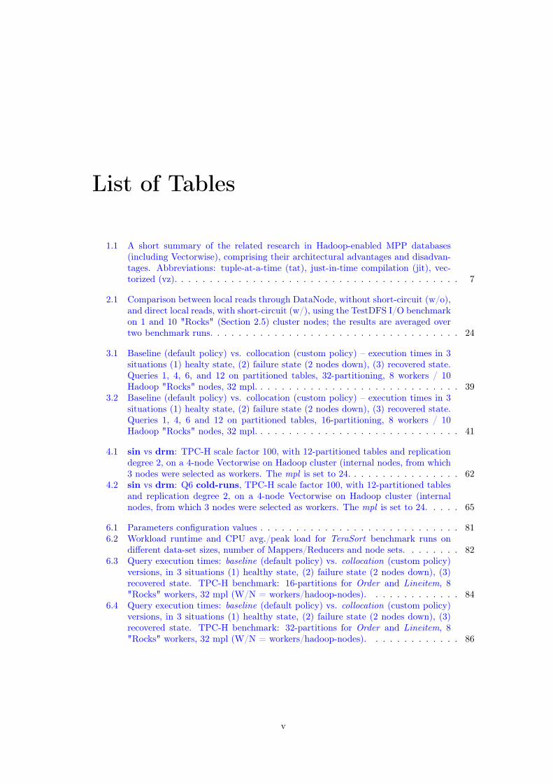
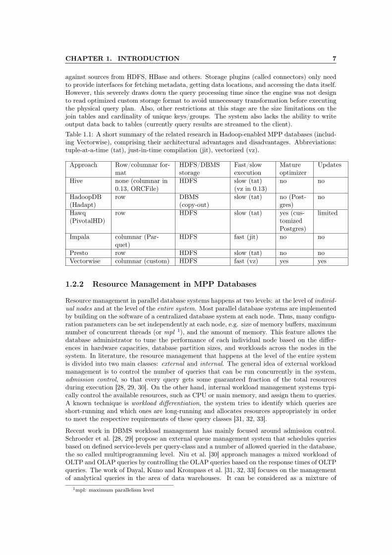
1.1 A short summary of the related research in Hadoop-enabled MPP databases(including Vectorwise), comprising their architectural advantages and disadvan-tages. Abbreviations: tuple-at-a-time (tat), just-in-time compilation (jit), vec-torized (vz). . . . . . . . . . . . . . . . . . . . . . . . . . . . . . . . . . . . . . . . 7
2.1 Comparison between local reads through DataNode, without short-circuit (w/o),and direct local reads, with short-circuit (w/), using the TestDFS I/O benchmarkon 1 and 10 "Rocks" (Section 2.5) cluster nodes; the results are averaged overtwo benchmark runs. . . . . . . . . . . . . . . . . . . . . . . . . . . . . . . . . . . 24
3.1 Baseline (default policy) vs. collocation (custom policy) – execution times in 3situations (1) healty state, (2) failure state (2 nodes down), (3) recovered state.Queries 1, 4, 6, and 12 on partitioned tables, 32-partitioning, 8 workers / 10Hadoop "Rocks" nodes, 32 mpl. . . . . . . . . . . . . . . . . . . . . . . . . . . . . 39
3.2 Baseline (default policy) vs. collocation (custom policy) – execution times in 3situations (1) healty state, (2) failure state (2 nodes down), (3) recovered state.Queries 1, 4, 6 and 12 on partitioned tables, 16-partitioning, 8 workers / 10Hadoop "Rocks" nodes, 32 mpl. . . . . . . . . . . . . . . . . . . . . . . . . . . . . 41
4.1 sin vs drm: TPC-H scale factor 100, with 12-partitioned tables and replicationdegree 2, on a 4-node Vectorwise on Hadoop cluster (internal nodes, from which3 nodes were selected as workers. The mpl is set to 24. . . . . . . . . . . . . . . . 62
4.2 sin vs drm: Q6 cold-runs, TPC-H scale factor 100, with 12-partitioned tablesand replication degree 2, on a 4-node Vectorwise on Hadoop cluster (internalnodes, from which 3 nodes were selected as workers. The mpl is set to 24. . . . . 65
6.1 Parameters configuration values . . . . . . . . . . . . . . . . . . . . . . . . . . . . 816.2 Workload runtime and CPU avg./peak load for TeraSort benchmark runs on
different data-set sizes, number of Mappers/Reducers and node sets. . . . . . . . 826.3 Query execution times: baseline (default policy) vs. collocation (custom policy)
versions, in 3 situations (1) healthy state, (2) failure state (2 nodes down), (3)recovered state. TPC-H benchmark: 16-partitions for Order and Lineitem, 8"Rocks" workers, 32 mpl (W/N = workers/hadoop-nodes). . . . . . . . . . . . . 84
6.4 Query execution times: baseline (default policy) vs. collocation (custom policy)versions, in 3 situations (1) healthy state, (2) failure state (2 nodes down), (3)recovered state. TPC-H benchmark: 32-partitions for Order and Lineitem, 8"Rocks" workers, 32 mpl (W/N = workers/hadoop-nodes). . . . . . . . . . . . . 86
v

LIST OF TABLES vi
6.5 Query execution times during node failures: colloc. without dynamic resourcemanagement (not. collocation) vs. colloc. with dynamic resource manage-ment (not. drm). TPC-H benchmark: 16-partitions for Order and Lineitem,8 "Rocks" workers, 32 mpl, 0.25 core over-allocation, RMax resp. degree 2.Since RMax = 2 we can form two separate worker-subsets. In (a) we fail 1worker from a subset and 1 from the other, in (b) we fail 2 workers from justone of the subsets. . . . . . . . . . . . . . . . . . . . . . . . . . . . . . . . . . . . 88
6.6 Query execution times without Hadoop busyness, no overlapping external work-loads: testing Vectorwise without YARN integration (not. drm) vs. with YARNintegration (not. drmy). TPC-H benchmark: Q1 and Q13 hot-runs, 32-partitionsfor Order and Lineitem, 8 "Stones" workers, 128 mpl, no core over-allocation,RMax resp. degree 2. . . . . . . . . . . . . . . . . . . . . . . . . . . . . . . . . . . 92
6.7 Query execution times during overlapping external (Hadoop) workloads, 16 Map-pers / 16 Reducers: testing Vectorwise without YARN integration (not. drm)vs. with YARN integration (not. drmy). TPC-H benchmark: Q1 and Q13 hot-runs, 32-partitions for Order and Lineitem, 8 "Stones" workers, 128 mpl, no coreover-allocation, RMax resp. degree 2. . . . . . . . . . . . . . . . . . . . . . . . . . 93
6.8 Query execution times during overlapping external (Hadoop) workloads, 32 Map-pers / 32 Reducers: testing Vectorwise without YARN integration (not. drm)vs. with YARN integration (not. drmy). TPC-H benchmark: Q1 and Q13 hot-runs, 32-partitions for Order and Lineitem, 8 "Stones" workers, 128 mpl, no coreover-allocation, RMax resp. degree 2. . . . . . . . . . . . . . . . . . . . . . . . . . 94
6.9 Query execution times during overlapping external (Hadoop) workloads, 64 Map-pers / 64 Reducers: testing Vectorwise without YARN integration (not. drm)vs. with YARN integration (not. drmy). TPC-H benchmark: Q1 and Q13 hot-runs, 32-partitions for Order and Lineitem, 8 "Stones" workers, 128 mpl, no coreover-allocation, RMax resp. degree 2. . . . . . . . . . . . . . . . . . . . . . . . . . 95

Chapter 1
Introduction
1.1 Background and Motivation
In the recent past of Big Data Analytics many companies shifted from a "one size fits all"software stack towards a data-pipeline composed of new generation technologies deployed oncommodity clusters, a collaborative approach where workloads were naturally served to theplatform that handles them best. Typically, there are two categories of big-data platformsthat could be used to build a data-pipeline for storing and processing huge amounts of data,either structured or unstructured. The first category includes MPP1 analytical databases thatare designed to store huge amount of structured data across a cluster of servers and performfast parallel queries over it. Most of the MPP solutions follow a shared nothing architecture,which means that every node will have a dedicated disk, memory, processor, and a high speednetwork connection. As these databases are designed to hold structured data, there is a needto extract the structure from raw data using an ETL2 tool. This is where Hadoop 3, the secondcategory, comes into help. Apache Hadoop is unquestionably the "de facto" platform for big-data environments. It is a system for distributing computation among cluster nodes, which, atits core, consists of HDFS 4 and the Map-Reduce framework 5. The latter is a computationalapproach [1] that involves breaking large volumes of data down into smaller batches, and pro-cessing them separately. A cluster of compute nodes, each one built on commodity hardware,scan multiple batches and aggregate data. Then the nodes’ output is shuffled and merged intothe final result. We will invariably find Hadoop working as part of a system with an MPPdatabase, because big-data solutions do not fall entirely into either structured or unstructureddata categories. Therefore, when combined altogether, this kind of big-data pipeline becomesessentially a connector-based system approach where Hadoop is used to extract structure fromdata and then load it into the MPP database’s own custom format storage in order to enablefast analytical query execution. In practice, this signifies having connectors in place to shipdata back and forth over network between the Hadoop and MPP database separate environ-ments. But, given that both systems handle data at their best, there is a lot more to gain ifwe perceive them as a single ecosystem. Nowadays, simply no one wishes to begin its big-datajourney with two logically separate systems. Connectors between Hadoop and MPP databaseclusters are quickly going to disappear. Many organizations working on big-data already oughtto have an easy to manage data platform that can support complex analytical query workloads,but also batch processing of unstructured data, free-text searches, graph analysis and whatever
1MPP: massively parallel processing2ETL: extract transform load3Apache Hadoop: hadoop.apache.org4HDFS: Hadoop Distributed File System, hortonworks.com/hadoop/hdfs5Map-Reduce: wiki.apache.org/hadoop/MapReduce
1

CHAPTER 1. INTRODUCTION 2
else may come up in the future. For that purpose, the industry is standardizing on Hadoopas the unifying infrastructure, since MPP clusters are generally non-standardized systems anddifficult to configure and manage. There is a tremendous interest in leveraging the Hadoopecosystem instead, trying to make MPP solutions converge around its HDFS and YARN 1 [4]infrastructure, and thus coexist with a Hadoop cluster. This shift to modern MPP databases ontop of Hadoop opens at least two new research directions: using HDFS for storage managementand YARN for resource management. The first one, brings MPP databases the support to runquery workloads directly on top of HDFS stored tables, using on-disk custom file formats. Thistopic has been receiving a lot of attention lately, from projects such as Parquet [2] and ORC-File [3]. On the other hand, the second direction is less explored (or not at all). Nevertheless,it is as equally important as storage management and they both work in tandem if we thinkabout data-locality and failover aspects. Resource management, if tackled from the right angle,can give us the advantage of sharing the same cluster resources between different applicationplatforms (e.g. Map-Reduce jobs and query workloads), and most importantly, it will complywith Hadoop’s standards and its system administrators’ know-how.
Therefore, the main question we address in this thesis is: How can we efficiently share computeresources within a Hadoop environment? More specifically, how can we share compute resourcesbetween an MPP analytical database and other computing frameworks, like Map-Reduce, inorder to achieve good utilization within the same Hadoop cluster? Not for so long, Apachestarted to address this question in their undergoing YARN [4] project (as part of HadoopNextGen), which enables resource management for heterogeneous parallel applications runningin a Hadoop cluster. In older Hadoop release versions, the scheduler was purely a Map-Reducejob scheduler. If you wanted to run multiple parallel computation frameworks on the samecluster, you would have to statically partition all the resources or hope that the same resourcesgiven to a Map-Reduce job would not have also been allocated by another framework’s sched-uler, causing Operating Systems to thrash. With YARN’s new design, the scheduler can nowhandle compute resources for different applications (mixed-workloads) running on the samecluster, which should allow for more multi-tenancy and a richer, more diverse Hadoop ecosys-tem. Therefore, our research focus is to achieve dynamic resource management in Vectorwiseon Hadoop 2.
1.2 Related Work
To offer a better understanding of our research topic, we start this section with a short overviewof the few most important key features in large-scale data analytics system, as introduced in [5].This is just an attempt to cover the design principles and core features of a database system froma wide perspective, filling the gap between the more classical category and the new Hadoop-enabled category (SQL-on-Hadoop). We then describe some of the technological innovationsin Hadoop-enabled MPP architectures that have each spawned a distinct (product) system fordata analytics. The last part of this section draws the attention towards resource managementin MPP databases and in a Hadoop environment. We focus on systems for large-scale dataanalytics, namely, the field that is called Online Analytical Processing (OLAP) as opposed toOnline Transaction Processing (OLTP).
Data Model. A data model provides the definition and the logical structure of the data, anddetermines in which manner it can be stored, organized, and manipulated by the system. Themost popular example of a data model supported by most parallel database systems is therelational model (which uses a table-based format), with its row-based or the more advancedcolumnar storage formats, whereas most systems in the Map-Reduce categories permit data to
1YARN: Yet Another Resource Negotiator2Vectorwise on Hadoop (Prject Vortex) presentation: www.slideshare.net/Hadoop_Summit/actian-vector-
on-hadoop-first-industrialstrength-dbms-to-truly-leverage-hadoop
CHAPTER 1. INTRODUCTION 3
be handled in any arbitrary format, even flat files. A relational database consists of relations(or, tables) that, in turn, consist of tuples. Every tuple in a table conforms to a schema whichis defined by a fixed set of attributes. The data model used by each system is closely related tothe query interface exposed by the system, which allows users to manage and manipulate thestored data.
Storage Layer. At a high level, a storage layer is simply responsible for persisting the data aswell as providing methods for accessing and modifying the data. The design, implementationand features provided by the storage layer used by each of the different system categories varygreatly, especially as we start comparing systems across the different categories. For example,classic parallel databases use integrated and specialized data stores that are tightly coupled withtheir execution engines, whereas Map-Reduce systems typically use HDFS as an independentdistributed file-system for accessing data. Only recently, with the outcome of Hadoop-enabledarchitectures, MPP database systems started to leverage HDFS as their native storage layer,using columnar data formats [2, 3] that are specifically tailored for its I/O capabilities.
Query Optimization. In general, query optimization is the process a system uses to determinethe most efficient way to execute a given query by generating several alternative, yet equivalent,execution plans. The techniques used for query optimization in the systems we consider arevery different in terms of: (i) the space of possible execution plans (e.g. relational operatorsin databases versus configuration parameter settings in Map-Reduce systems), (ii) the type ofquery optimization (e.g. cost-based versus rule-based), (iii) the type of cost modeling technique(e.g. analytical models versus models learned using machine-learning techniques), and (iv) thematurity of the optimization techniques (e.g. fully automated versus manual tuning).
Query Execution. When a database system receives a query for execution, it will mostlyconvert it into a physical plan for accessing and processing the query’s input data. The executionengine is the entity responsible for actually running a given execution plan in the system andgenerating the query result. Most query interpreters follow the so-called Volcano iterator-model [6], in which each operator implements an API that consists of open(), next() and close()methods. In the original proposal, the next() call produces a tuple-at-a-time. The queryevaluation follows a pull model : the next() operator is applied recursively on the operator treefrom the root downwards, while the resulted tuples being pulled upwards.
However, it has been observed that the tuple-at-a-time model leads to interpretation overhead:the situation that much more time is spent in evaluating the query plan than in actuallycalculating the query result, affecting the recent innovations in modern CPUs [7]. MonetDB [8]reduced this overhead by using bulk processing instead, making each operator fully processits input and only then invoke the next execution stage. This idea has been further improvedin the X100 project [9] and later evolved into vectorized execution, a form of block-orientedquery processing [10] in which the next() method produces small (typically 100-10000) single-dimensional arrays of tuples (called vectors), rather than a single tuple. This type of tuplerepresentation is easily accessible for modern CPUs and has the consequence that the percentageof instructions spent in interpretation logic is reduced by a factor equal to the vector-size [11].Another popular method used by today’s execution engines in order to eliminate the overheadof interpretation is just-in-time query compilation. Upon receiving a query for the first time, thequery processor compiles (a part of) the query into a routine that gets subsequently executed.Query compilation removes the interpretation overhead altogether. A compiled code can alwaysbe made faster than an interpreted code and it is reusable for queries that are repeated withdifferent parameters.
In the MPP systems that we consider, the execution engine is also responsible for parallelizingthe computation across large-scale clusters of machines and setting up inter-machine commu-nication to make efficient use of the network and disk bandwidth. The final execution plan iscomposed of operators that support both intra-operator and inter-operator parallelism, as wellas mechanisms to transfer data from producer operators to consumer operators.
CHAPTER 1. INTRODUCTION 4
Scheduling. Given the distributed nature of most data analytics systems, scheduling thequery execution plan makes it an important part of the system. Systems must now take severalscheduling decisions, including scheduling where to run each computation, scheduling inter-nodedata transfers, as well as scheduling rolling updates and maintenance tasks.
Resource Management. Resource management primarily refers to the efficient and effectiveuse of a cluster’s resources based on the resource requirements of the queries or applicationsrunning in the system. In addition, many systems today offer elastic properties that allow usersto dynamically add or remove resources as needed according to workload requirements.
Scheduling and resource management are not only important, but also very challenging. Clus-ters are exposed to a wide range of applications, that have highly diverse characteristics andperformance requirements. For example, Map-Reduce applications are usually characterized bylong running jobs. These jobs desire shorter turnaround time - time from submission to com-pletions. Queries in database systems for analytical or transactional workloads, on the otherhand, are much shorter-lived and much more interactive. Further, these environments need tosupport a large number of users simultaneously. As a result, the underlying system needs torespond to these kind of workloads as soon as they arrive, even at the cost of stretching theiroverall turnaround time slightly. Managing both types of workloads at the same time makesit even more difficult for a cluster resource manager, especially when each workload belongsto a different applications (e.g. running Map-Reduce jobs and OLAP queries). Schedulingand resource management needs to take numerous system parameters, such as CPU speed,memory size, I/O bandwidth, network bandwidth, context switch overhead, etc, into account.These metrics are often inter-related and can affect the choice of an effective scheduling strat-egy. Depending on the characteristics of the system (on-line vs off-line, closed vs open, etc)and the nature of the jobs/queries (preemptive vs non-preemptive, service times with knownor unknown distribution, prioritized vs equal jobs, etc), several static and dynamic schedulingalgorithms have been proposed [12]. In parallel database systems, however, the consensus isthat dynamic load-balancing is mandatory for effective resource utilization [13, 14]. Variousalgorithms have been proposed for these kind of systems depending on the different levels ofparallelism: inter-transaction, inter-query, inter-operator and intra-operator parallelism [15].
Failover. Machine failures are relatively common in large clusters. Hence, most systems havebuilt-in failover functionalities that would allow them to continue providing services, possiblywith performance degradation, in the face of unexpected events like hardware failures, softwarebugs, and data corruption. Examples of typical failover features include restarting failed tasks(or services) either due to application or hardware failures, recovering data due to machinefailure or corruption, and using speculative execution to avoid stragglers.
System Administration. System administration refers to all tasks where additional humaneffort may be needed to keep the system running while the system serves the needs of multipleusers and applications. Common activities under system administration include performancemonitoring and tuning, diagnosing the cause of poor performance or failures, capacity planning,and system recovery from temporary and permanent failures (e.g. failed disks).
1.2.1 Hadoop-enabled MPP Databases
In this section we discuss the research in the literature that constitutes the state of the artin Hadoop-enabled MPP databases. A summary of the system’s architectural advantages anddisadvantages is given in Table 1.1.
Hive. One of the first initiatives (in 2008) to bring the familiar concepts of tables, columns,partitions and a subset of SQL to the unstructured world of Hadoop is Hive [16], an open-sourcedata warehousing solution built entirely on top of Hadoop and HDFS. Hive supports queriesexpressed in a SQL-like declarative language called HiveQL statements, which are compiled

CHAPTER 1. INTRODUCTION 5
and broken down into individual Map-Reduce jobs that are later executed with Hadoop. WithHiveQL users can also plug in custom Map-Reduce scripts into their queries. The languageincludes a type system with support for tables containing primitive types and as well as morecomplex collections like arrays, maps and structs. The latter ones can be nested arbitrarilyin order to construct more complex compositions. Hive also includes a system catalog calledMetastore that is stored on HDFS and contains table schemas and statistics, useful in dataexploration, query optimization and query compilation. The underlying IO libraries can beextended to query data in custom formats, thus allowing users to implement their own types andfunctions. Even so, the HDFS data files do not have a custom storage format, nor a row-basedor columnar-based, which makes the query execution very slow and inefficient. Moreover, Hivedoes not support in-memory buffering/caching mechanisms. It is known to be a one-at-a-timedata analysis framework, where the data has to be read from disk and parsed again each timea user performs a query; HDFS tuples cannot be passed as intermediate results. The per-queryMap-Reduce overhead prevents the ability of this technology to process queries interactively,placing Hive in the "batch processing" category of computational frameworks. Yet, with thedelivery of the Stinger project 1 in June 2014, the last Hive release (Hive 0.13) got enhanced withcolumnar storage, more intelligent data placement to improve scan performance, and vectorizedexecution [17]. Besides, on the project’s roadmap one of the goals was also to integrate Hivewith Tez 2, a modern implementation of Map-Reduce that allows interactive queries (reducingthe processing overhead) and in-memory materialized results.
HadoopDB. HadoopDB [18] is another example of an open source Hadoop-enabled databaseproject, initiated at Yale in 2009, whose architecture is of a hybrid system. The basic ideabehind HadoopDB is to use Map-Reduce as the communication layer above multiple nodesrunning single-node DBMS instances. Queries are expressed in SQL, translated into Map-Reduce by extending the existing Hive components, and as much work as possible is pushedinto the underlying layer of database; the rest of the query is processed using the more genericMap-Reduce framework. For a Map-Reduce job in order to communicate with the databaselayer the authors implemented a custom database connector – an interface between independentdatabase instances and TaskTrackers, usually mapped 1-to-1 on any node in the cluster. So,each Map-Reduce job supplies the connector with SQL query and connection parameters suchas: which JDBC driver to use, query fetch size and other query tuning parameters. The con-nector connects to the database, executes the SQL query and returns results as key-value pairs.Therefore, HadoopDB resembles a shared-nothing parallel database with Hadoop providingservices necessary for scalability. The creators of HadoopDB have since started a commercialsoftware company (Hadapt) to build a system that unites Hadoop/Map-Reduce and SQL, aPostgres database is placed in nodes of a Hadoop cluster. Altogether, combining Map-Reduceand Postgres has the following drawbacks. First, using Map-Reduce as the communicationslayer adds a big overhead to query execution and makes it very slow. In [19], for the authors’experimental setup, it takes an average of 35 seconds per query just to get it started. This is along-standing complaint about Map-Reduce: high-latency, batch-mode response is painful forlots of applications that want to process and analyze data in critical time. Data communicationhappens via HDFS: latency is introduced as extensive network I/O is involved in moving dataaround, e.g. in the reduce phase. That aside, since there is a sort and shuffle phase after themap phase all the outputs always have to be sorted and sent to the reducers. So, the executiontime depends on the slowest phase among all three map, reduce and shuffle phases. Second,since Postgres needs to store data on local files we have to load all the data from HDFS to theengine’s storage system before running any queries. This makes loading data a cumbersomeslow process, a complete pre-load and data organization leads to the worst initial response timeof about 800 seconds [19]. On the other hand Postgres was not built with replication in mind(is not relying on HDFS for that purpose), which means HadoopDB cannot handle failoversand so, the database’s availability has to suffer in case of failures.
1Stinger project: hortonworks.com/labs/stinger2Tez: hortonworks.com/hadoop/tez

CHAPTER 1. INTRODUCTION 6
Hawq. A commercial product that recently entered the MPP Hadoop-like database market isHawq [20, 21], a mix between EMC’s Greenplum [22] MPP database and Hadoop v2, part ofa new EMC on Hadoop stack called the Pivotal Hadoop Distribution. In contrast with Hive,Hawq tries to take all of the inherent scalability and replication benefits from HDFS; it doesnot embrace a Map-Reduce execution style nor the Hive’s query engine, or other friendly query-interfaces for Hadoop. The system allows to be queried with any standard SQL syntax or anytool that speaks SQL, using a custom query engine based on Greenplum MPP engine (a matureoptimized version of Postgres engine). Also, Hawq’s approach is different from HadoopDB’sinvisible loading [19]. The invisible loading algorithm "invisibly" rearranges data from slow,file-system style data layout to fast, relational data-layout. In Hawq, the same data is pulledfrom HDFS into Greenplum’s execution engine every time, i.e. if data is stored as a flat file inHDFS, then when the query is over, it will still be stored as a flat file in HDFS. However, theannouncement out of Hawq Pivotal HD is still a port of a decade-old technology (meaning theGreenplum’s customized Postgres database) that is albeit rather slow for OLAP queries, has itsown, independent, non-integrated schema metadata layer which cannot share information withthe rest of the Hadoop platform (it exists only on the Master node, the workers are stateless),and supports just limited update and delete operations (e.g. single row update/delete).
Impala. One of the main contributors of the Hadoop project, Cloudera, has been developing aswell a distributed parallel SQL query engine that blends into Hadoop’s stack, turning it into areal-time fault-tolerant distributed query engine. The Impala [23] query engine can run directlyon top of HDFS, enabling users to issue low-latency SQL queries on data stored in HDFS usingcustom formats, such as Parquet columnar storage format [2], or the HBase tabular overlay.All these changes bring Impala closer to the Hadoop ecosystem. With Impala, Cloudera isbasically replacing parts of Hive’s and HBase’s components with custom built ones, while stillbeing compatible with Hive and HBase APIs. The result is that large-scale data processing (viaMap-Reduce) and interactive queries can be done on the same system using the same data andmetadata, removing the need to migrate data sets into specialized database storage systemsand/or proprietary formats simply to perform analytical queries. The underlying SQL engine inImpala is not reliant on Map-Reduce as Hive is, but rather on a single-core (lack of parallelism)distributed database stack that has a new query planifier, a new query coordinator, and a newquery execution engine. Furthermore, as an improvement to the last component (the queryexecution engine), Impala uses just in time query compilation [24]. This significantly improvesthe CPU efficiency, plus the overall query execution time, and outperforms the traditionalinterpreted query processing with tuple-at-a-time execution [25]. However, since Imapala isstill at the first release versions, it does not have a query optimizer, nor a mature executionengine yet. For instance, the QET 1 currently limits the execution level of subqueries, usuallyfixed at 2 or 3 levels deep, and won’t generate plans that are arbitrarily deep. Also, addingthat Hadoop v2 was released in October 2013, it lacks of YARN integration.
Presto. Presto [26] is a distributed SQL query engine developed by Facebook and optimized forad-hoc analysis at interactive speed. The execution model of Presto is fundamentally differentfrom Hive [27], which translates queries into multiple stages of Map-Reduce tasks that executeone after another and each one reads inputs from disk and writes intermediate output back toit. In contrast, the Presto engine does not use Map-Reduce. It employs a custom query andexecution engine with operators designed to support SQL semantics. In addition to improvedscheduling, all processing is in memory and pipelined across the network between stages. Thisavoids unnecessary I/O and associated latency overhead. The pipelined execution model runsmultiple stages at once, and streams data from one stage to the next as it becomes available.This significantly reduces end-to-end latency for many types of queries. The Presto system isimplemented in Java and certain portions of the query plan are dynamically compiled downto byte code which lets the JVM optimize and generate native machine code. Presto wasdesigned with a simple storage abstraction that makes it easy to provide SQL query capability
1QET: query execution tree
CHAPTER 1. INTRODUCTION 7
against sources from HDFS, HBase and others. Storage plugins (called connectors) only needto provide interfaces for fetching metadata, getting data locations, and accessing the data itself.However, this severely draws down the query processing time since the engine was not designto read optimized custom storage format to avoid unnecessary transformation before executingthe physical query plan. Also, other restrictions at this stage are the size limitations on thejoin tables and cardinality of unique keys/groups. The system also lacks the ability to writeoutput data back to tables (currently query results are streamed to the client).Table 1.1: A short summary of the related research in Hadoop-enabled MPP databases (includ-ing Vectorwise), comprising their architectural advantages and disadvantages. Abbreviations:tuple-at-a-time (tat), just-in-time compilation (jit), vectorized (vz).
Approach Row/columnar for-mat
HDFS/DBMSstorage
Fast/slowexecution
Matureoptimizer
Updates
Hive none (columnar in0.13, ORCFile)
HDFS slow (tat)(vz in 0.13)
no no
HadoopDB(Hadapt)
row DBMS(copy-out)
slow (tat) no (Post-gres)
no
Hawq(PivotalHD)
row HDFS slow (tat) yes (cus-tomizedPostgres)
limited
Impala columnar (Par-quet)
HDFS fast (jit) no no
Presto row HDFS slow (tat) no noVectorwise columnar (custom) HDFS fast (vz) yes yes
1.2.2 Resource Management in MPP Databases
Resource management in parallel database systems happens at two levels: at the level of individ-ual nodes and at the level of the entire system. Most parallel database systems are implementedby building on the software of a centralized database system at each node. Thus, many configu-ration parameters can be set independently at each node, e.g. size of memory buffers, maximumnumber of concurrent threads (or mpl 1), and the amount of memory. This feature allows thedatabase administrator to tune the performance of each individual node based on the differ-ences in hardware capacities, database partition sizes, and workloads across the nodes in thesystem. In literature, the resource management that happens at the level of the entire systemis divided into two main classes: external and internal. The general idea of external workloadmanagement is to control the number of queries that can be run concurrently in the system,admission control, so that every query gets some guaranteed fraction of the total resourcesduring execution [28, 29, 30]. On the other hand, internal workload management systems typi-cally control the available resources, such as CPU or main memory, and assign them to queries.A known technique is workload differentiation, the system tries to identify which queries areshort-running and which ones are long-running and allocates resources appropriately in orderto meet the respective requirements of these query classes [31, 32, 33].
Recent work in DBMS workload management has mainly focused around admission control.Schroeder et al. [28, 29] propose an external queue management system that schedules queriesbased on defined service-levels per query-class and a number of allowed queried in the database,the so called multiprogramming level. Niu et al. [30] approach manages a mixed workload ofOLTP and OLAP queries by controlling the OLAP queries based on the response times of OLTPqueries. The work of Dayal, Kuno and Krompass et al. [31, 32, 33] focuses on the managementof analytical queries in the area of data warehouses. It can be considered as a mixture of
1mpl: maximum parallelism level

CHAPTER 1. INTRODUCTION 8
external and internal workload management. Besides admission control based on extensivequery run-time prediction, they additionally control the execution of queries and propose thepossibility to kill long running queries in case higher priority queries are present.
Another important dimension of resource management is how the system can scale up in orderto continue to meet performance requirements (quality of service) as the system load increases.The load increase may be in terms of the size of input data stored in the system and processedby queries, the number of concurrent queries that the system needs to run, the number ofconcurrent users who access the system, or some combination of these factors. The objectiveof shared-nothing parallel systems is to provide linear scalability. For example, if the inputdata size increases by 2x, then a linearly-scalable system should be able to maintain the currentquery performance by adding 2x more nodes. Partitioned parallel processing is the key enablerof linear scalability in parallel database systems. One challenge here is that data may have tobe repartitioned in order to make the best use of resources when nodes are added to or removedfrom the system.
1.2.3 Resource Management in Hadoop Map-Reduce
We now briefly review some of the related work about resource management in a Hadoop(Map-Reduce) environment. There have been several efforts that investigate efficient resourcesharing while considering fairness constraints. For example, Facebook’s fairness scheduler [34]aims to provide fast response time for small jobs and guaranteed service levels for productionjobs by maintaining job "pools" each of which is assigned a guaranteed minimum share andby dividing excess capacity among all jobs or pools. Yahoo’s capacity scheduler [35] supportsmulti-tenancy by assigning capacities to different job queues, so each job queue gets a fair shareof the cluster resources. Zaharia et al. [36] developed a scheduling algorithm called LATE thatperforms effective speculative execution to reduce the job running time in Hadoop heteroge-neous environments; it uses the estimated remaining execution time of tasks as the guidelineto select tasks to speculate and avoids assigning speculative tasks to slow nodes. However,without a data-locality aware placement scheme, previously mentioned approaches have onlylimited opportunities for optimizations during task placement. To improve data-locality, sev-eral enhancements have been proposed. In an environment where most jobs are small, delayscheduling [37] can improve data-locality by delaying the scheduling of tasks that cannot achievedata-locality by a short period of time. This seems a simple technique to provide better lo-cality, but it does not consider global scheduling, and so it loses the opportunity for achievingbetter overall performance. Purlieus [38] tries to solve the fundamental problem of optimizingdata placement so as to obtain local execution of the jobs during scheduling, minimizing thecross-rack traffic during both map and reduce phases. To do so, it categorizes Map-Reducejobs into three classes: map-input heavy, map-and-reduce-input heavy and reduce-input heavy,and proposes data and virtual machine placement strategies accordingly to minimize the cost ofdata shuffling between map tasks and reduce tasks. Similar in approach is CAM [39], a topologyaware resource manager for Map-Reduce applications in the cloud that also proposes a threelevel approach to avoid placement anomalies due to inefficient resource allocation: placing datawithin the cluster that run jobs that most commonly operate on the data, selecting the mostappropriate physical nodes to place the set of virtual machines assigned to a job and exposing,otherwise hidden, compute, storage and network topologies to the Map-Reduce job scheduler.CAM uses a minimum-cost flow network based algorithm that is able to reconcile resource al-location with a variety of other constraints, such as storage utilization, changing CPU load andnetwork link capacities. Unlike Purlieus, CAM’s minimum-cost flow based approach is able toconsiders both VM migration as well as delayed scheduling to arrive at a global optimal place-ment. Quincy [40] is a Dryad resource scheduler for concurrent jobs that tackles the conflictbetween data-locality and fairness by converting the scheduling problem to a graph that en-codes both network structure and waiting tasks and solving it with a minimum-cost flow solver.

CHAPTER 1. INTRODUCTION 9
Though it uses similar graph techniques, it differs from CAM in terms of problem space andassociated flow network construction. Quincy balances between fairness and data-locality, whileCAM focuses on optimizing data/VM placement of Map-Reduce applications in the cloud. Asa result, the factors encoded in the flow graph (VM closeness, etc.) are quite different fromthat of Quincy’s.
However, not all these ideas (described above) are suitable for a Hadoop-enabled MPP architec-ture. At least three assumptions considered by some of the authors are not applicable to thesearchitectures: (1) workloads can be delayed, and so the waiting time can be taken into accountwhen scheduling and managing compute resources, (2) only Map-Reduce workloads run in aHadoop cluster (multi-tenancy is not considered), and (3) job profiling can be done beforehandon a small subset of data in order to categorize the workload from the I/O-, CPU-, network-perspective.
1.2.4 YARN Resource Manager (Hadoop NextGen)
In the previous Hadoop version (v1), figure 1.1a, each node in a cluster was statically assigneda predefined number of map and reduce slots for running map and reduce tasks altogether [?],meaning that the allocation of cluster resources to Map-Reduce jobs was done in the form ofthese slots. This static allocation model had the obvious drawback of lowered cluster utilization,since slot requirements vary during a Map-Reduce job life cycle. There is a high demand formap slots when the job starts, whereas there is a similar demand for reduce slots towards theend. However, the simplicity of this scheme facilitated the resource management performedby the Job Tracker, in addition to the scheduling decisions. Hadoop Job Tracker had multipleroles, such as managing the cluster resources as well as scheduling, monitoring, and managingthe life-cycle of Map-Reduce jobs. On the other hand, the Task Tracker had fewer and simplerresponsibilities, such as starting/tearing-down or pinging the job-application to check if it isstill alive. Hadoop NextGen (v2), figure 1.1b, also known as YARN [4], separates the abovefunctionalities into: a global Resource Manager (RM), responsible for allocating resources torunning applications, a per-application Application Master (AM) to manage the application’slife-cycle, including its resource requests towards RM, and also a per-machine Node Manager(NM) to handle the user processes and the available resources of that node. The AM is aframework-specific library that negotiates resources from the RM and works with the NM(s) toexecute and monitor an application’s set of tasks. To build a custom YARN Application fromscratch a user needs to implement the API of the YARN Client Application. The transition fromHadoop v1 to NextGen v2 is depicted in figure 1.1. Historically, Map-Reduce applications werethe only ones that could have been managed by Hadoop (v1) at that time, due to its limitedresource management capabilities. Today, due to YARN’s new design, Map-Reduce is just one ofHadoop’s application frameworks. Hadoop NextGen permits building and deploying distributedapplications using other frameworks as well, see figure 1.1c. The resource allocation scheme inYARN addresses the static allocation issues of the later Hadoop version by introducing the ideaof resource containers. A container represents a specification of a node compute resources (orattributes), such as CPU, memory, and in future, disk and network bandwidth. In this model,only a minimum and a maximum for each attribute are defined, and AMs can request differentcontainer sizes at different times with attribute values as multiples of the minimum. Therefore,YARN provides resource negotiation and management for the entire Hadoop cluster and allthe applications running on it. This leaves us the believe that, once integrated with YARN,non-Hadoop distributed applications (e.g. Vectorwise query workloads) can run as first-classcitizens on Hadoop clusters by sharing resources side-to-side with Hadoop-native applications.

CHAPTER 1. INTRODUCTION 10
(a) Job submission in Hadoop v1
(b) Job submission in Hadoop v2
(c) Hadoop stack: v1 to v2
Figure 1.1: Hadoop transition from v1 to v2

CHAPTER 1. INTRODUCTION 11
1.3 Vectorwise
Vectorwise 1 is a state-of-the-art relational database management system that is primarilydesigned for online analytical processing, business intelligence, data mining and decision supportsystems. The typical workload of these applications consists of many complex (computationallyintensive) queries against large volumes of data that need to be answered in a timely fashion.What makes the Vectorwise DBMS unique and successful is its vectorized, in-cache executionmodel that exploits the potential performance of modern hardware (e.g. CPU cache, multi-coreparallelism, SIMD instructions, out-of-order execution) in conjunction with a scan-optimizedI/O buffer manager, fast transactional up dates and a compressed NSM/DSM storage model [7].
The Volcano Model. The query execution engine of Vectorwise is designed according to thewidely-used Volcano iterator model [6]. A query execution plan is represented as a tree of opera-tors, hence often referred to as a query execution tree (QET). Operators are an implementationof constructs responsible for performing a specific step of the overall required query processing.All operators implement a common API, providing three methods: open(), next() and close().Upon being called on some operator, these methods recursively call their corresponding meth-ods on the QET’s children operators, starting from the root operator downwards. The open()and close() are one-off complementary methods that perform initialization work and resourcerelease, respectively. Each next() call produces a new tuple (or a block of tuples, see Vector-ized Query Execution below). Due to the recursive nature of the next() call, query executionfollows a pull model in which tuples traverse the operator tree from the leaf operators upwards,at the root operator the final results being returned. The benefits of using such a model in-clude flexibility and extensibility, as well as a demand-driven data flow that guarantees thatthe whole query plan is executed within a single process and without unnecessary intermediatematerialized data.
Multi-core Parallelism. Vectorwise (single-node SMP version) is capable of multi-core paral-lelism in two forms: inter-query parallelism and intra-query parallelism. The latter is achievedthanks to a special operator of the Volcano model, called the Xchange operator (not. Xchg) [41].
Vectorized Query Execution. It has been observed that the traditional tuple-at-a-timemodel leads to low instruction and data cache hit rates, wasted opportunities for compileroptimizations, considerable overall interpretation overhead and, consequently, poor CPU uti-lization. The column-at-a-time model, as implemented in MonetDB [8] successfully eliminatesinterpretation overhead, but at the expense of increased complexity and limited scalability, dueto its full-column materialization policy.
The execution model of Vectorwise combines the best of these two features by adapting theQET operators in order to process and return not one, but a fixed number of tuples (from100 - 10000, default is 1024) whenever the next() method is called. This block of tuples isreferred to as a vector and the number of tuples is chosen such that the vector can fit in theL1-cache memory of a processor. The processing of vectors is done by specialized functionscalled primitives. This reduces the interpretation overhead of the Volcano model, because theinterpretation instructions are amortized across multiple tuples and the actual computationsare performed in tight loops, thus benefiting from the performance features of modern CPUs(e.g. superscalar CPU architecture, instruction pipelining, SIMD instructions) [7], as well ascompiler optimizations (e.g. loop unrolling).
The rest of this section is organized as follows. We first give an overview of the Ingres-Vectorwisedesign in Section 1.3.1. Next, in Section 1.3.2, we discuss the distributed Vectorwise MPPdatabase version. Last but not least, Section 1.3.3 presents the Hadoop-enabled (Vectorwise onHadoop) architecture.
1Vectorwise website: www.actian.com/products/vectorwise

CHAPTER 1. INTRODUCTION 12
1.3.1 Ingres-Vectorwise Architecture
Vectorwise is integrated within the Ingres 1 open-source DBMS. A high-level diagram of thewhole system’s architecture, showing the main architectural components, is depicted in Figure1.2.
Ingres is responsible for the top layers of the database management system stack. The Ingresserver interacts with users running the Ingres client application and parses the SQL queriesthey perform. Also, Ingres keeps track of the database schemas, metadata and statistics (e.g.cardinality, distribution) and uses this information for computing and providing to Vectorwisean optimal query execution plan. Vectorwise can be seen as the database system’s engine,being responsible for the whole query-tree execution, buffer management and storage. Its maincomponents are described below.
Client Application
SQL Parser
Optimizer
Rewriter
Builder
Query Execution Engine
Buffer Manager
Ingr
esVe
ctor
wis
e
data request
physical operator tree
annotated plan (VW alg.)
query plan (VW alg.)
parsed tree
client query (SQL)
resu
lts
data
I/O request data
Storage
resource management (VW alg.)
Figure 1.2: The Ingres-Vectorwise (single-node) High-level Architecture
Rewriter. The optimized query execution plans that Ingres passes to Vectorwise are expressedas logical operator trees in a simple algebraic language, referred to as the Vectorwise Algebra.The Rewriter performs specific semantic analysis on the received query plan, annotating it withdata types and other helpful metadata. It also performs certain optimization steps that werenot done by Ingres, such as introducing parallelism, rewriting conditions to use lazy evaluationand early elimination of unused columns.
Builder. The annotated query plan is then passed to the Builder, which is responsible forinterpreting it and producing a tree of physical operators that implement the iterator function-ality of the Volcano model. The latter (producing the physical tree) corresponds to calling theopen() method on all operators in a depth-first, post-order traversal of the query execution tree.Also, this is when most of the memory allocation and initialization takes place.
Query Execution Engine. Once the builder phase is done and the physical operator treeis constructed, executing the query then simply translates to repeatedly calling next() on theroot operator of the tree until no more tuples are returned. The paragraphs on the VolcanoModel and Vectorized Query Execution should have given a good description of the way theVectorwise query execution engine works.
1Ingres website: www.actian.com/pro ducts/ingres

CHAPTER 1. INTRODUCTION 13
Buffer Manager and Storage. The Buffer Manager and Storage layer is primarily responsiblefor storing data on persistent media, accessing it and buffering it in memory. Additionally, italso takes care of handling updates, managing transactions, performing crash recovery, logging,locking and more.
Resource Manager. When a query is received in (the SMP single-node version of) Vectorwise,an equal-share of resources is allocated (at the beginning) for it. This amount of resources,namely the number of threads, is called the maximum parallelism level and it is calculatedas the maximum number of cores available (possibly multiplied by an over-allocation factor)divided by the number of queries running in the system. Then, when transformations areapplied, the MPL is used as an upper bound to the number of parallel streams in generatedquery plans. Finally, once the plan with the best cost is chosen, the state of the system isupdated.
The reason behind an equipartition strategy for resource management is that the queries pro-cessed by the execution engine are all independent, their service time distribution is unknownand differences in workloads may be significant. Moreover, queries have different degrees of re-source utilization and of parallelism at different levels of the query plan. It has been proven thatit can be an efficient strategy for different class of workloads and service time distributions [42],which is the typical case for Vectorwise queries.
The information about the number of queries running in the system and the number of coresused by each query is stored in the Resource Manager’s state. Note that this information is amere approximation of the CPU utilization. Depending on the stage of execution and/or thenumber and size of the Xchg operator’s buffers, a query can use less cores than the numberspecified, but it can also use more cores for shorter periods of time.
1.3.2 Distributed Vectorwise Architecture
Most organizations demand from their OLAP capable DBMS systems a small response time toqueries on volumes of data that increases at a constant pace. In order to comply with theserequirements, the most successful commercial database service providers have developed MPPdatabase solutions meant to run on supercomputers or clusters.
The Vectorwise SMP product, though is successful in achieving high performance, low cost andusability, its ability to handle large amounts of data is limited by the fact that it is designed towork on a single machine. The research developed in the master-thesis project [43] shows howthis version can be enriched with distributed query processing capability, such that it can bedeployed on a computer cluster. To achieve this, both the query execution engine and the queryoptimizer had to be extended with new functionality, while maintaining the original qualities.
Figure 1.3 presents the high-level architecture of the distributed Vectorwise MPP database asit was designed and implemented by the authors of [43], currently Actian software engineers.The architecture relies on a "Virtual" Shared Disk storage layer and follows a Master-Workerpattern, in which the Master node is the single point of access for client applications. Themain advantage of a Master-Worker design is that it hides from clients the fact that the DBMSthey connect to actually runs on a computer cluster. The Shared Disk (SD) approach waspreferable, opposed to Shared Nothing (SN), for ensuring non-intrusiveness, ease of use andmaintainability. The main difference between both, SD vs SN, architectures is whether or notexplicit data partitioning is required. SD does not require it, as every node of the cluster hasfull access to read and write against the entirety of the data. On the other hand, the latterstatement does not hold in the case of a SN architecture and additional effort is required fordesigning a partitioning scheme that minimizes inter-node messaging, for splitting data amongthe cluster nodes and for implementing a mechanism to route requests to the appropriatedatabase servers. For a more elaborated comparison we recommend reading the second chapter

CHAPTER 1. INTRODUCTION 14
of [43], the author’s chosen "Approach" for their research project. The general idea is that, withgood partitioning schemes, function- and data-shipping can be avoided for most query patterns,leading to optimal results in terms of performance. The big challenge is, however, devising sucha good partitioning scheme and maintaining it automatically, without user intervention, byregularly re-partitioning and re-balancing data across the cluster nodes. While this is indeedone of the major goals in the quest towards the distributed MPP version of Vectorwise, it wasa too complex task to tackle in a master-thesis project.
Because of the design choice, it is hence inevitable that the Master node must become involvedin all queries issued to the system, in order to gather results and return them to clients, atleast. However, as can be seen in the architecture diagram, it has more than one task assigned,making it the only node responsible for:
• parsing SQL queries and optimizing query plans
• keeping track of the system’s resource utilization, as it has knowledge of all queries thatare issued to the system
• taking care of scheduling / dispatching queries, based on the above information
• producing the final, annotated, parallel and possibly distributed query plans
• broadcasting them to all worker nodes that are involved
The Vectorwise MPP database is intended for highly complex queries across large volumes ofdata. In this situation, the vast majority of the total query processing time is spent in the queryexecution stage. Parallelizing the latter is enough for achieving good speedups and performingthe before-mentioned processing steps sequentially is acceptable. Moreover, depending on thesystem load and scheduling policy, the Master may also get involved in query execution to alarger extent than simply producing the distributed plan and gathering the query results.
Client Application
SQL Parser
Optimizer
Rewriter
Builder
Query Execution Engine
Buffer Manager
Ingr
esVe
ctor
wis
e
data request
physical operator tree
annotated plan (VW alg.)
query plan (VW alg.)
parsed tree
client query (SQL)
resu
lts
data
Builder
Query Execution Engine
Buffer Managerdata request
physical operator tree
data
annotated
plan (VW alg.)
Storage ("Virtual" Shared Disk)
Vectorwise
I/O request dataI/O request data
Worker Node
dataexchange
Mas
ter N
ode
resource management (VW alg.)
Figure 1.3: The Distributed Vectorwise High-level Architecture
For a distributed Vectorwise MPP solution, the following modules of the single-node versionneeded to be modified or extended:
Rewriter. A new logical operator (called Distributed Exchange) was introduced in queryplans, which completely encapsulates parallelism and distribution. The transformations of the

CHAPTER 1. INTRODUCTION 15
parallel rules and the operators’ costs were adapted too. The new distributed plan containsboth intra-operator and inter-operator parallelism, as well as mechanisms to transfer data fromproducers to consumers. Also, in order for this module to be cluster-aware, the Rewriterrequests information about the current state of the cluster (e.g. the number of cores availableon each node, number of running threads, etc) from the Resource Manager.
Builder. Every node is able to build its corresponding parts of a query execution tree andphysically instantiate each new operators. Since a single node can run several parts of thequery, is required for the Builder to produce a forest of sub-trees, rather than a single rootedtree.
Execution Engine. The Distributed Exchange operator was implemented in a way to allowthe Master and various Workers to efficiently cooperate (e.g. exchange data, synchronize) whenexecuting a given query. After the execution of a query is finished, this module will releaseresources in a parallel fashion, similar to the idea employed in the (parallel) Builder, and theninform the Resource Manager about that. For the network-communication layer it was decidedto rely on the MPI (Message Passing Interface) library, which is considered to be the "de-facto" standard for communication among process that model a parallel program running on adistributed memory system. No other changes were made at this layer.
Resource Manager. Besides the existent functionality of the the single-node Resource Man-ager, two new policies for query scheduling were introduced for the distributed version of Vec-torwise: the single-node and multiple-nodes distribution policies.
The single-node distribution policy (no-distribution) tries to keep the network traffic at a mini-mum and, at the same time, process linearly more queries than the single-node DBMS version.It does so by processing each query on a single node and then communicating the results throughthe Master node, to the client. The idea behind this policy is to choose one single node that isthe least loaded one in the cluster, calculate the mpl relative to the node, apply the transfor-mations to generate a parallel query plan that should run entirely on that machine and, finally,add a DXchg(1:1) operator on top of it, if necessary. This operator sends the results to theMaster node so that can be sent to the client.
On the other hand, the multiple-nodes distribution policy aims to produce distributed queryplans that give a good throughput performance in a multi-user setting. It is an extension of thepolicy used in the non-distributed DBMS: a single DXchg operator that works at the granularityof threads. This policy unifies the resources available on the cluster and shares them equallybetween concurrent queries. Then, the task is to find the smallest set of least loaded nodes thatcan provide the required parallelism level. For every node in this set, the query is allocatedall the cores on that node, with possibly one exception (when the remaining parallelism levelrequired is in fact smaller than the number of cores on that node).
In order to determine the load of a particular node, a state of the system has to be maintained,just like in the non-distributed version of the Vectorwise DBMS. As all of the queries areexecuted through the Master node, it makes sense to keep this information up-to-date there.To determine on which node to run a received query, the Master node assigns a load factor toevery node in the cluster:
Li = wt ∗ Ti + wq ∗Qi,
where:
• Ti is the thread load on node i. It is defined as the estimated total number of threadsrunning on i divided by the number of available cores on i.
• Qi is the query load on node i and it is defined as the number of running queries on idivided by the total number of running queries in the system. This value and the threadload are the only available information about the state of the system. Since the thread

CHAPTER 1. INTRODUCTION 16
load is only an approximation (no real usage, e.g. percentage information) of the currentutilization of a particular node, the query load becomes a complement of it and acts as atiebreaker in some cases (e.g. when the thread load is equal, the node with less queriesrunning is chosen).
• wt and wq are associated weights, with wt + wq = 1 (experimentally determined).
1.3.3 Hadoop-enabled Architecture
Vectorwise has been now extended to bring its data analytics performance to Hadoop. It hasa mature RDBMS engine that can perform SQL processing of data stored natively in HDFS, arich SQL language support, unique update capabilities, and an advanced query optimizer. TheHadoop-enabled architecture aims to scale-out Vectorwise on top of Hadoop/HDFS in order toprovide a general-purpose, high-performance, Big Data Analytics product.
High-level overview
The core of the Hadoop-enabled version is the distributed Vectorwise MPP engine, which isbased on the research work from [43]. We briefly remind that the authors of [43] have designedand implemented a solution for distributed (multi-core parallel) queries using a "Virtual" SharedDisk approach. Although the file system the authors used (GlusterFS 1) did not performed asexpected, they were nevertheless able to prove their core concepts.
The HDFS layer is also perceived as a "Virtual" Shared Disk. However, each node in thecluster has its own (physically separated) set of disks and that gives better I/O performancefor local- data accesses over remote- ones. Using partitioned tables with block location affinityin HDFS we can achieve a more flexible shared-nothing and performant system. Therefore,this makes our new (Vectorwise on Hadoop) approach a combination of a "Virtual" Shared diskwith partitioning and affinity. The Hadoop-enabled architecture, figure 1.4, still follows thetraditional Master-Worker pattern. Whenever the database restarts, a new session is initiatedand one of the X100 backend workers is elected as the session-master (or Vectorwise Master)without any additional actions. This session is kept alive during the whole lifespan of theVectorwise database to let the Vectorwise Master fulfill its responsibilities, see Section 1.3.2.Within a Hadoop cluster, the NameNode can serve as a node location for Ingres and theVectorwise Master, if not involved in query processing, and (just a designated subset of) theDataNodes can serve, respectively, for the Vectorwise Workers. Otherwise, if the session-masteris involved in query execution, there would be no difference as such in the node locations becauseevery X100 processes must then have access to a local DataNode (for short-circuit local reads).In the hindmost case, the NameNode will share the same location with on of the DataNodes,as illustrated in Figure 1.4. We further refer to the designated subset of nodes starting the(session of) X100 backend processes as the Vectorwise worker-set. Given that a large-scaleHadoop cluster can have nodes with various hardware configurations, the worker-set concept isintroduced to help us on selecting (throughout a process that is described in Section 4.1) a setof machines with identical capabilities and thus, achieve a better load-balancing. While it isrecommended to have Vectorwise X100 servers installed on many of the DataNodes as possible,in order to chose at will on which nodes we should run the database, is not necessary that allservers should be used at once. The choice of HDFS keeps the system simpler and, though inprinciple each worker can see the entire system state because of its global (remote) access, itenables us to fall back into single-writer algorithms for update operations. It also enables easyimplementation of failover functionalities, since in general, if performance is not considered forremote data accesses, no data needs to be moved in case the worker-set changes.
1GlusterFS website: www.gluster.org

CHAPTER 1. INTRODUCTION 17
Figure 1.4: The Vectorwise on Hadoop High-level Architecture (the session-master, or Vector-wise Master, is involved in query execution).
To offer a better understanding of what is special about Vectorwise on Hadoop, let us reviewsome of the new key concepts introduced in the Hadoop-enabled architecture:
Basic partitioned table support. One thing to take into account, in order to have scalabilityon large joins, is that all-to-all communication between the Vectorwise worker nodes must beavoided – even Infiniband networks will not support the speed of Vectorwise joins, and ina typical Hadoop scenario we just have a 10Gb Ethernet network. Therefore, some kind ofpartitioning or clustering is needed that allows to execute joins and aggregation locally on eachworker. The idea is to introduce table partitioning that splits a logical table into multiplephysical tables on HDFS using hash-partitioning on a column (or a set of columns). Everypartition has in principle one responsible worker, and that is the worker which stores (locally)the first replica of that partition. Still, this mapping is not strict, if a node goes down wecan make another node responsible for its table partitions. We explain in Chapter 4 moreabout the previous situation and how it can change if we take as well in account the secondarypartition replicas. Table partitioning is introduced during bulk-loading, where each worker getsdata determined by a partitioning key. Partitioning is physically implemented by adding uniontables to Vectorwise, which is a virtual table (view) made up by the union of physical tablepartitions. Besides hash-partitioned (collocated) tables, Vectorwise on Hadoop supports global(non-partitioned) tables as well. The latter of the two, are in-memory (all over the worker-set)cached tables used in general for performing local shared-HashTable hash-joins.
HDFS Database Locations. To store data on HDFS we do need to define a directory struc-ture, a hierarchy of locations to which we can store separately (and isolate) one database’s files
CHAPTER 1. INTRODUCTION 18
(logs, tables, metadata, profiles, etc.) from another. Each Vectorwise on Hadoop session startswith a database location, an HDFS path where log files, global (non-partitioned) tables, catalogmetadata, etc. are stored (e.g. hdfs:///location/name). A database location generally points toa list of table locations – of which only one is the default location and set to hdfs:///<databaselocation>/default, whereas the others are defined per table during schema creation. The listof table locations is written in a metadata file and stored at the Vectorwise database location.Beside all these, there is also a local (non-HDFS) work location that is used for disk– sortingand spilling.
Columnar HDFS storage model. The parallel-rewriter has a rule that transforms a data-loading query having a cluster-load (cluster VWLoad) operator into a distributed query plan,where each node loads into a specified partition of the table. The data is distributed by hashingon key columns. We assume that data is stored in HDFS in multiple files and each file containsdata for just a single column. For the cluster VWLoad queries, the rewriter associates files toload operators in a round-robin fashion. However, files may have affinities to particular nodes(and there should be a way of detecting these affinities using the HDFS library). Therefore, infuture stages, files will be assigned to operators with affinity. The VWLoad operator used to be(in the single-node version) a utility component in the client-space, a command-line client usedto parse and send data through a TCP connection to the local X100 server. Nowadays, in thedistributed MPP version, these functionalities have been separated from the utility componentand redesigned into a query operator instead. For parsing and loading the data into HDFS, thisoperator forks a helper (JVM) process that communicates through Unix pipes with the X100(parent) backend process.
Supporting Updates in HDFS, via Positional Delta Trees (PDTs). Vectorwise im-plements a fully ACID–compliant transactional database with multi-version read consistency.Any new transaction will see all previously committed transactions, both small incrementaltransactions and large bulk data loads. Changes are always written persistently to HDFS intoa write ahead transaction log (WAL) before a commit completes. This will always ensure fulltransaction recoverability. Nonetheless, one of the biggest challenges with HDFS is that it is notdesigned for incremental updates. HDFS files are append-only and so, in place updates are notallowed. Vectorwise on Hadoop addresses this challenge with its high-performance in-memoryPositional Delta Trees [44] (PDTs), which are used to store small incremental changes (insertsthat are not appended), as well as updates and deletes. Conceptually, a PDT is an in-memorystructure that stores the position and the change (delta) at that position and permit queriesto efficiently merge the PDTs changes with the HDFS stored data. Because of the in-memorynature of PDTs, small DML statements can be processed very efficiently. A background pro-cess writes the in-memory changes to disk once a memory threshold is exceeded. Important tomention is that only the session-master writes to the WAL (PDTs on-commit). The WAL fileis read-only for the Workers and read-write for the Master. At startup, each worker reads the(global accessible) WAL, but skips the PDTs on the partitions it is not responsible for. If anupdate is triggered, then the worker nodes will ship their local PDTs changes over the networkto the session-master, who finally writes all these changes to the WAL.
Query plan on logically partitioned tables. For the query-plan search strategy, the existentapproach uses the resource scheduler developed in the MSc thesis [43]. For each new query,the algorithm provides us a list of pairs (nx, ty) denoting how many threads/cores (ty) areallocated for its execution on node (nx). In order to restrict the search strategy from tryingall possible combinations of threads/node (which will lead to an exponential complexity), weneed to accept the following: (a) assuming that partitions will be created with almost equalsizes, it only makes sense to try to assign an equal number of resources (in our case threads)to each partition, (b) for every partition, there will be at least one thread assigned to it; ifthis restriction is not set, there would be cases in which a thread will be assigned to scanmultiple partitions. The search starts with a feasible (initial) solution and tries all its multiples(e.g. [(1, 3), (2, 5)] : [(1, 6), (2, 10)] : [(1, 9), (2, 15)] : etc . . .). It stops at the first combination
CHAPTER 1. INTRODUCTION 19
which needs more threads (on any machine) than allocated by the resource scheduler. Theimplementation adds two new multiple-nodes distribution policies for queries: (1) equal-sharefor non-partitioned – similar with the multiple-nodes distribution used in the Shared Diskapproach it selects the least loaded nodes and takes their amount of CPU resources until itsatisfies the mpl and (2) equal-share for partitioned tables – it assumes the default round-robinpartitioning and equally assigns threads to the operators until the mpl is achieved. However,ideally would be to balance the assignment with respect to data-locality (i.e. local partitions)and each node’s load factor (i.e. overloaded worker nodes).
Ingres client side mpi_fork and worker-set selection. In Vectorwise on Hadoop, theIngres client should query YARN Resource Manager and see which nodes are alive in the cluster.Once we have selected the most resourceful N worker nodes from the entire Vectorwise cluster(consisting of M nodes, M can be equal to N) and have reserved the initial amount of resources(CPU and memory), we can then start the X100 worker-set using an mpi_fork command.For the worker-set initialization process we assume (and is important) that the assignment ofpartitions across the nodes, i.e. the exact node-locations of each partition, is already known. Werefer to this assignment in the next paragraphs as the responsibility assignment, or the node’sresponsibilities. Knowing the latter information, each of the X100 backend servers can replaythe LOG and skip PDTs, MinMax and Join -Indexes for all the partitions that do not correspondto them (or, better said, that is not responsible of). Among all the worker nodes, only one ischosen to be the Master. This node is the one to receive the sequential query (algebra) planand rewrite it into a distributed parallel one. The final (best-cost) plan initiates the distributedexecution on top of the Vectorwise worker-set. Also, as we mentioned above, the Master nodeis the only one that can change/update the WAL file and handle non-partitioned tables. Sofar, there is no automatic approach to select the nodes participating in the worker-set. To starta Vectorwise on Hadoop cluster, human intervention is currently needed to explicitly specifythe worker nodes. Hence, due to the lack of this feature, the existent Vectorwise on Hadooparchitecture cannot handle transparent failovers and so, it cannot reassign the responsibilitiesof the failed nodes to the remaining nodes in the worker-set. This process should be handledtransparently by querying the HDFS NameNode to find out where the partitions are locatedand, using this information to determine the missing replicas, have them re-replicated to other(new) nodes.
1.4 Research Questions
We now address the most important questions related to dynamic resource management inVectorwise on Hadoop MPP database:
• What metric sets (application, cluster, node -specific metrics) from YARN Resource Man-ager can be used to manage a parallel database system, likewise Vectorwise on Hadoop?
• How can we get our metric sets and inform YARN about a specific resource allocation(e.g. nodes’ locations, number of cores, amount of memory)?
• What is the granularity of resources that we can claim with YARN?
• How can we use data-locality to influence YARN’s resource allocation?
• What algorithms to compute node assignments are appropriate for us, in three situations:
1. to determine the initial Vectorwise worker-set?
2. to dynamically reassign responsibilities to worker-set at startup time (e.g. in case ofa node failure)?
3. to determine the optimal subset of workers to run a particular query?

CHAPTER 1. INTRODUCTION 20
• What are the challenges in dynamic resource management for Hadoop-enabled MPPdatabase technologies?
1.5 Goals
Through the planning and development stages of our project, we have been seeking to create aprototype that:
• is in control of the HDFS replication layer and always keeps the data local to the workernodes, especially after node failures when missing replicas have to be re-replicated to other(new) nodes
• transparently handles failovers by reassigning the responsibilities of the failed nodes to theremaining nodes (or new ones) in the worker-set, such that the load is spread as evenlyas possible with respect to data-locality
• increases the performance during failovers, favoring local-reads over remote-reads
• achieves dynamic resource management, with focus on load-balancing and resource uti-lization
• is integrated with YARN, aiming towards an elastic approach to increase/decrease theresource requirements
1.6 Basic ideas
The outline below is meant to give the reader an idea of the directions according to which theproject/prototype was carried out:
• control data-locality by instrumenting the HDFS block placement policy
• implement an algorithm to decide node responsibilities at startup with respect to data-locality and load-balancing factors
• similarly, decide the subset of nodes and the amount of resources we can use to run aquery; we refer to it as the resource footprint (or the resource requirements) of a Vectorwisequery
• use YARN to acquire/release resources within the Hadoop ecosystem
Implementation constraints
• requires easy and non-intrusive modifications to the current implementation
• requires no additional effort in order to configure and use it
• adds no overhead to the rewriter, builder and query execution

Chapter 2
Approach
This chapter presents a high-level overview of the main components and algorithms we imple-mented in order to enable dynamic resource management in Vectorwise on Hadoop, and alsoexplains how various design choices were made in accordance with the research questions of thisproject. The rationale behind the "Basic Ideas" presented in Section 1.6 should become clearby the end of this chapter.
To begin with, for a cost-effective, scalable, yet efficient solution, we focused our attention to-wards the open-source Apache Hadoop v2.2 (YARN) 1, which we have installed and configuredon two independent sets of cluster nodes with different hardware configuration, but all intercon-nected by a low-latency, high bandwidth network fabric. Section 2.1 elaborates on the choicefor HDFS direct local reads (short-circuit reads). In Section 2.2 we argue that instrumentingthe block-placement policy in Hadoop is preferable to ensure data-locality, not only after databulk-loading, but also after data re-replication (i.e. HDFS recovery phase) due to node failures,ease of use (i.e. no additional configurations) and maintainability (i.e. increasing/decreasingthe worker-set and automatically moving data during a file-system check). In Section 2.3 webriefly describe the algorithms for dynamic resource management in Vectorwise on Hadoop. InSection 2.4 we present the solution space behind a good integration of long-running application-s/jobs with Yarn and the high-level overview of our chosen approach for Vectorwise, mentioningthe architectural components and their work-flow to acquire/release resources. Finally, moredetails about our experimentation platform / cluster’s hardware specs are found in Section 2.5.
Below, in Figure 2.1, we illustrate our research approach (and the project’s contributions)in 7 steps, more or less in the order of their development: (1) start Vectorwise database,(2) select the worker-set and assign (partition) responsibilities, (3) generate metadata, (4)store metadata file in HDFS, (5) instrument HDFS block replication, (6) get cluster resourceinformation and (7) acquire/release resources through YARN. These steps are going to beintroduced by the remaining of the section and their goal should be clear by the end of readingit. Nevertheless, we do reserve a chapter for each of the most important topics: Chapter 3for instrumenting HDFS block replication, Chapter 4 for dynamic resource management (i.e.worker-set selection, responsibility assignment, computing the worker-set resource footprint)and Chapter 5 for YARN integration. Last but not least, Chapter 6 highlights some of theresults we achieved during this research project.
1Hadoop v2.2 (YARN) release: hadoop.apache.org/docs/r2.2.0/
21
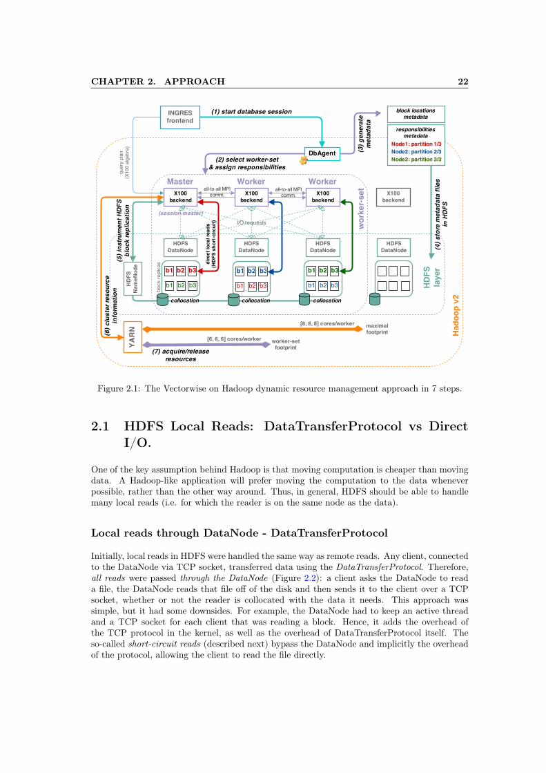
CHAPTER 2. APPROACH 22
Figure 2.1: The Vectorwise on Hadoop dynamic resource management approach in 7 steps.
2.1 HDFS Local Reads: DataTransferProtocol vs DirectI/O.
One of the key assumption behind Hadoop is that moving computation is cheaper than movingdata. A Hadoop-like application will prefer moving the computation to the data wheneverpossible, rather than the other way around. Thus, in general, HDFS should be able to handlemany local reads (i.e. for which the reader is on the same node as the data).
Local reads through DataNode - DataTransferProtocol
Initially, local reads in HDFS were handled the same way as remote reads. Any client, connectedto the DataNode via TCP socket, transferred data using the DataTransferProtocol. Therefore,all reads were passed through the DataNode (Figure 2.2): a client asks the DataNode to reada file, the DataNode reads that file off of the disk and then sends it to the client over a TCPsocket, whether or not the reader is collocated with the data it needs. This approach wassimple, but it had some downsides. For example, the DataNode had to keep an active threadand a TCP socket for each client that was reading a block. Hence, it adds the overhead ofthe TCP protocol in the kernel, as well as the overhead of DataTransferProtocol itself. Theso-called short-circuit reads (described next) bypass the DataNode and implicitly the overheadof the protocol, allowing the client to read the file directly.

CHAPTER 2. APPROACH 23
Figure 2.2: Local reads through DataNode (DataTransferProtocol).
Figure 2.3: Direct local reads (Direct I/O - open(), read() operations).
Direct local reads – Direct I/O
The key idea behind short-circuit local reads (Figure 2.3) boils down to the following: if aclient runs on the same node with its data, there is no need to involve the DataNode in thereading path. Rather, the client itself can simply read the data from the local disk using directI/O primitives, open() and read() operations. Obviously, this is only possible in cases wherethe client is collocated with data. Short-circuit reads provide a substantial performance boostto many applications and so we have enabled this option in all our performance tests. Thisperformance optimization made it into Hadoop v2.2 (YARN) as well 1. To configure short-circuit local reads, you will need to enable libhadoop.so. Short-circuit reads make use of aUNIX domain sockets. This is a special path in the filesystem that allows the client and theDataNodes to communicate. You will need to set a path to this socket and the DataNode needsto be able to create this path. On the other hand, it should not be possible for any user exceptthe HDFS user or root to create this path, for security concerns. For this reason, paths under/var/run or /var/lib are often used.
A short comparison between the two of these read options, reads through DataNode and short-circuit reads, is shown in Table 2.1. We can see from the results that, even though the map-readers access only local data, with short-circuit reads (direct local reads) the I/O throughputboosts in performance by 5-15% for both single file – single map-reader and also multiple files– multiple map-readers tests.
1Short-circuit local reads configuration: hadoop.apache.org/docs/r2.2.0/hadoop-project-dist/hadoop-hdfs/ShortCircuitLocalReads.html

CHAPTER 2. APPROACH 24
Table 2.1: Comparison between local reads through DataNode, without short-circuit (w/o),and direct local reads, with short-circuit (w/), using the TestDFS I/O benchmark on 1 and 10"Rocks" (Section 2.5) cluster nodes; the results are averaged over two benchmark runs.
TestDFSIO | Reads w/o w/o w/ w/Number of files (1 per mapper): 1 10 1 10
Total MB processed: 10000 10000 10000 10000Throughput MB/s: 94.75 57.88 98.78 64.75
Average IO rate MB/s 94.75 63.61 98.78 67.60IO rate std deviation: 0.0132 19.6334 0.0182 15.3133Test exec time (s): 135.294 51.403 126.225 41.605
2.2 Towards Data Locality
As mentioned in 1.3.3 each node loads data into specific partitions of the table, based on thequery plan (VWLoad operators) that is rewritten by the parallel-rewriter. Tuples are distributedby hashing on key columns and stored in multiple HDFS files, where each file contains datafor just a single column of a partition – a Vectorwise (table) partition has as many HDFSfiles as columns in the logical table and one single file may require more than an HDFS block(default size is 128 MB) for storage. HDFS uses a simple policy to store replicas for a block.If a process that is running on any of the HDFS cluster nodes opens a file for writing a block,the first replica of that block is stored on the same machine which the client is running on(we call it first-write data-locality). The second replica is placed on a randomly chosen rackthat is different from the rack on which the first replica was written. Then, the third replica isstored on a randomly chosen machine from the same remote rack that was chosen in the firststep. This means that a block is present on two unique racks. One point to note is that thereis no relationship between replicas of different blocks of the same file as far as their locationis concerned. Each block is stored independently. On one hand, the algorithm is very simpleand yet good for availability and scalability. On the other hand, there are obvious cases wherecollocating blocks of the same file on the same set of datanode(s) or rack(s) is beneficial forperformance reasons. For instance, from a Map-Reduce application construct, if many blocks ofthe same file are found on the same datanode, a single mapper instance could process all theseblocks using the CombineFileInputFormat operator. Similarly, if a dataset contains many smallfiles that are collocated on the same datanode(s) or rack(s), one can use the same operator toprocess all these file together by using fewer mapper instances. Moreover, if an applicationalways uses one dataset in combination with another dataset (e.g. think of join operations ontables), then collocating these two datasets on the same set of datanodes is beneficial.
HDFS Block Placement Policy. In Vectorwise on Hadoop VWLoad queries, the rewriterassociates files to load operators in a round-robin fashion keeping the first-write data-locality inplace. However, at scan time, files may have different affinities to particular nodes (and thereshould be a way of detecting these affinities using the HDFS library) due to a possible systemfailover. Likewise, in case of a failover scenario (i.e. a node crashes) the default re-replicationpolicy is triggered and so the first-write data-locality will be lost. Hence, our approach towardsachieving full data-locality is to control the HDFS block replication by ourselves. To do sowe can use the HDFS-385 1 feature, which is already part of HDFS since its 0.21 release.This improvement provides a way for the developer to write Java code, within the same HDFSnamespace, that can instrument the block placement policy and specify, directly for instance,what target nodes should be used to store one file’s blocks and their replicas. The HDFSAPI is currently incomplete and experimental in nature, but that is expected to change andbecome stable in the near future. The default behavior of the block placement policy can be
1HDFS-385: issues.apache.org/jira/browse/HDFS-385

CHAPTER 2. APPROACH 25
modified by extending the BlockPlacementPolicy abstract class 1 and pointing the new class tothe dfs.block.replicator.classname property in the HDFS configuration file.
To sum up, we have enhanced the default HDFS replication and implemented a custom blockplacement policy for Vectorwise partitioned tables. Our custom policy makes sure that all theHDFS blocks of a Vectorwise table partition (implicitly all columns of that table) are collocatedon R target nodes (R equal to the replication factor) that we specify in the global location-map file. This file is generated at startup by our Vectorwise-on-Hadoop DbAgent component(or simply called the DbAgent, Section 2.3) and contains the R node locations for all table’spartition. The end result is that multiple Vectorwise column format HDFS files are collocated onthe same set of nodes and that re-replication (the recovery phase) is now under the control of theglobal location-map whenever some nodes might fail. Besides, we have also extended the HDFSfile-system-check primitives to ease-up the system administration routines, i.e. a sysadmin cancheck if the node locations of Vectorwise HDFS blocks are consistent with the global location-map and if not, those blocks will be automatically moved to their right destination. Moredetails about the implementation can be read in Chapter 3.
Comparison with other column based HDFS formats (Parquet andORCFile)
Parquet [2] vs ORCFile [3]. Parquet’s configurations [47] allows storing columns in differentHDFS block sizes (the RowGroup can be up to 1GB [48]), in which respect it is superior toStinger’s 2 (Apache Hive’s v0.12 release name) ORCFile. ORCFile uses a relatively smallRowGroup (called Stripes), such that even when a subset of columns is scanned, I/O must beperformed for the whole file. Hence, Parquet, with its maximum RowGroup of 1GB, can storea RowGroup in 16 x 64MB HDFS blocks, such that there is still hope for certain queries, whichonly select a few columns, to read less than all 16 blocks.
Parquet Schema. We note that Parquet has a ProtocolBuffer-like data format which allowsto store nested data-models, which would be similar to multiple tables with a JoinIndex in-between (similar with TPC-H 3 Orders-Lineitem tables join in Vectorwise). Though this isoutside of our project scope, it would be an interesting challenge to re-interpret a Parquet fileinto a relational schema. Note that, one Parquet file would potentially map to multiple tablesconnected by a JoinIndex. Vectorwise would need C-code-extensions (in MScan operator) tobe able to read the Parquet format, aside of our custom columnar file format.
HDFS Block Locality. The current algorithm that analyzes block placement could be usedto start-up Vectorwise server nodes such that they become responsible mostly for local files (i.ein case of re-replication locality is lost on the new nodes). The Map-Reduce based writer willcreate some locality in Parquet files, in that the blocks belonging to the same RowGroup willhave been written by the same Reduce jobs, which means that the default HDFS policy willplace the first replica/copy on that same node together (i.e. first-write data-locality). However,the other HDFS copies will randomly be scattered. As such, when nodes from the originalMap-Reduce-set that wrote a specific file fail, it will be impossible for them to regain full I/Olocality. In that sense, the failover behavior of native Vectorwise columnar files will be betterthan Parquet.
For future work, experiments can be done by loading the Orders and Lineitem tables of TPC-Hinto ORCFile and Parquet using Map-Reduce writers, showing that: (1) ORCFile cannot avoidunnecessary I/O even when a subset of columns is scanned, (2) Parquet can do so, howevernot at a very fine-grained level (it will still read unnecessary data), (3) Parquet data-locality is
1BlockPlacementPolicy abstract class: grepcode.com/file/repo1.maven.org/maven2/org.apache.hadoop/hadoop-hdfs/0.22.0/org/apache/hadoop/hdfs/server/namenode/BlockPlacementPolicy.java
2Stinger initiative’s website: hortonworks.com/labs/stinger/3TPC-H benchmark’s website: www.tpc.org/tpch/
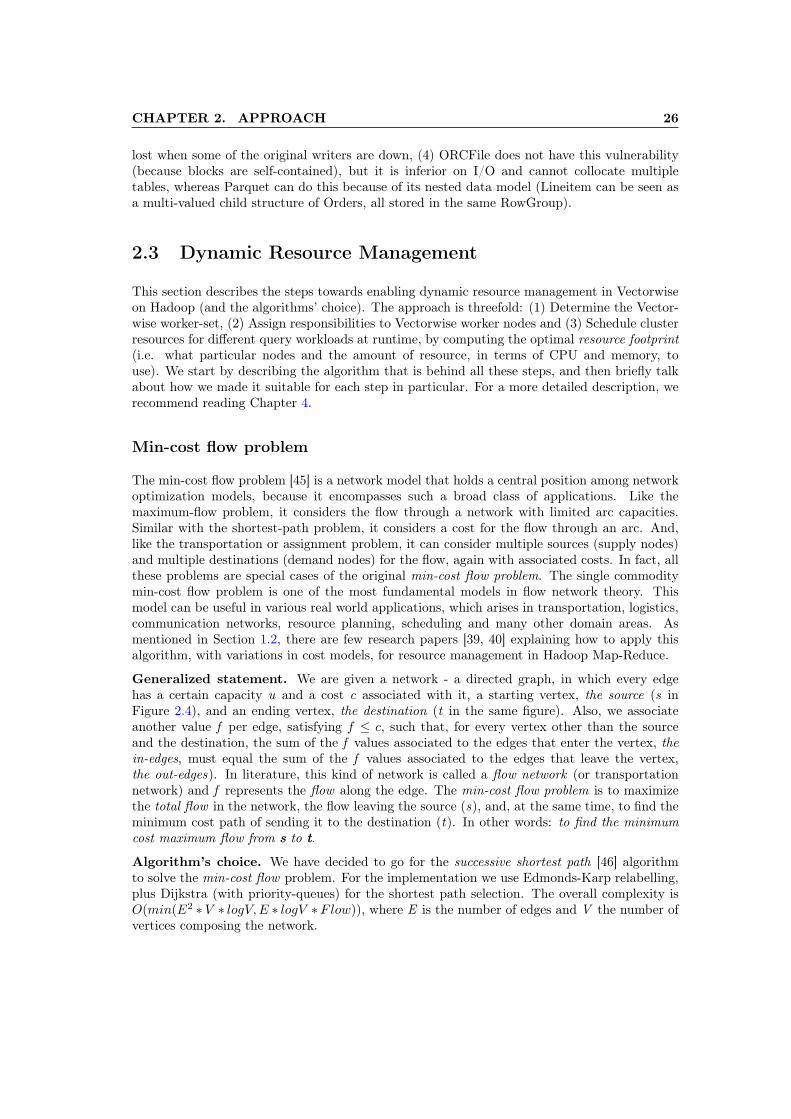
CHAPTER 2. APPROACH 26
lost when some of the original writers are down, (4) ORCFile does not have this vulnerability(because blocks are self-contained), but it is inferior on I/O and cannot collocate multipletables, whereas Parquet can do this because of its nested data model (Lineitem can be seen asa multi-valued child structure of Orders, all stored in the same RowGroup).
2.3 Dynamic Resource Management
This section describes the steps towards enabling dynamic resource management in Vectorwiseon Hadoop (and the algorithms’ choice). The approach is threefold: (1) Determine the Vector-wise worker-set, (2) Assign responsibilities to Vectorwise worker nodes and (3) Schedule clusterresources for different query workloads at runtime, by computing the optimal resource footprint(i.e. what particular nodes and the amount of resource, in terms of CPU and memory, touse). We start by describing the algorithm that is behind all these steps, and then briefly talkabout how we made it suitable for each step in particular. For a more detailed description, werecommend reading Chapter 4.
Min-cost flow problem
The min-cost flow problem [45] is a network model that holds a central position among networkoptimization models, because it encompasses such a broad class of applications. Like themaximum-flow problem, it considers the flow through a network with limited arc capacities.Similar with the shortest-path problem, it considers a cost for the flow through an arc. And,like the transportation or assignment problem, it can consider multiple sources (supply nodes)and multiple destinations (demand nodes) for the flow, again with associated costs. In fact, allthese problems are special cases of the original min-cost flow problem. The single commoditymin-cost flow problem is one of the most fundamental models in flow network theory. Thismodel can be useful in various real world applications, which arises in transportation, logistics,communication networks, resource planning, scheduling and many other domain areas. Asmentioned in Section 1.2, there are few research papers [39, 40] explaining how to apply thisalgorithm, with variations in cost models, for resource management in Hadoop Map-Reduce.
Generalized statement. We are given a network - a directed graph, in which every edgehas a certain capacity u and a cost c associated with it, a starting vertex, the source (s inFigure 2.4), and an ending vertex, the destination (t in the same figure). Also, we associateanother value f per edge, satisfying f ≤ c, such that, for every vertex other than the sourceand the destination, the sum of the f values associated to the edges that enter the vertex, thein-edges, must equal the sum of the f values associated to the edges that leave the vertex,the out-edges). In literature, this kind of network is called a flow network (or transportationnetwork) and f represents the flow along the edge. The min-cost flow problem is to maximizethe total flow in the network, the flow leaving the source (s), and, at the same time, to find theminimum cost path of sending it to the destination (t). In other words: to find the minimumcost maximum flow from s to t.
Algorithm’s choice. We have decided to go for the successive shortest path [46] algorithmto solve the min-cost flow problem. For the implementation we use Edmonds-Karp relabelling,plus Dijkstra (with priority-queues) for the shortest path selection. The overall complexity isO(min(E2 ∗ V ∗ logV,E ∗ logV ∗Flow)), where E is the number of edges and V the number ofvertices composing the network.

CHAPTER 2. APPROACH 27
Figure 2.4: A flow network example for the min-cost problem, edges are annotated with (cost,flow / capacity).
Worker-set selection & responsibility assignment
Worker-set selection. The idea is to select the best N nodes out of M with respect totheir resource (e.g. CPU, memory, etc) capabilities and local data, Vectorwise column formatHDFS local files, if any. This process is handled transparently by one of our components, theDbAgent : for the first part – getting the cluster’s capabilities – it asks YARN for the clusternode reports and for the second part – finding HDFS data – it queries the HDFS Namenodeand finds out where the Vectorwise files are located, assuming that the data was loaded intothe system beforehand. Moreover, based on the data-locality information, we can determinemissing replicas (i.e. in case of node failures) and have them re-replicated to other (possibly new)workers. The problem of (re)balancing table partitions to worker nodes, therefore creating theglobal location-map, can be stated as a min-cost matching problem 1 on a bipartite graph with acost model to reflect the (Vectorwise files’) data-locality to worker nodes (Chapter 4). As a sidenote, for the initial load we use a round-robin (horizontally) data partitioning scheme. However,following the initial load, the global location-map will always be re-generated according to thecurrent locations of the Vectorwise HDFS files (including their replicas) at startup time.
Responsibility assignment. There are multiple ways to decide which worker nodes areresponsible for specific partitions, depending on the HDFS replication degree. One-to-oneassignment – maximum one node responsible per partition: To assign responsibilities to workernodes, we apply the min-cost flow algorithm on a custom bipartite graph, Figure 2.5. The graphis structured in: (1) left-side : partitions and (2) right-side : workers. From our source (s) toeach partition, we connect edges with cost 0 and capacity RMax equal to 1 – Figure 2.5. Then,we connect edges from partitions to workers using a cost model that is explained in Chapter 4and capacity 1. Finally, we pair each worker to its destination node (t). We assign these edgesa cost 0 and a capacity equal to the partition-capacity of the worker we connect with (i.e.how many partitions a node can handle, annotated with PCap in the figure). Many-to-oneassignment – two or more nodes responsible per partition: This approach is similar with theprevious one, except one thing: the capacity of an edge connecting s with a partition, RMaxfrom Figure 2.5, is set to the maximum number of nodes responsible per partition.
Dynamic resource scheduling
To schedule resources for queries that run on (shared-nothing) partitioned tables, we haveenhanced the existent Vectorwise resource scheduler with a min-cost flow algorithm. For thismatter of problem, the algorithm uses a more advanced cost model (Chapter 4), though it isbased on a similar bipartite graph like the one used to assign responsibilities. We briefly remindthat, in the existent approach, the algorithm provides us a list of pairs (nx, ty) denoting how
1Note that the min-cost matching is just a specialization of the min-cost flow problem
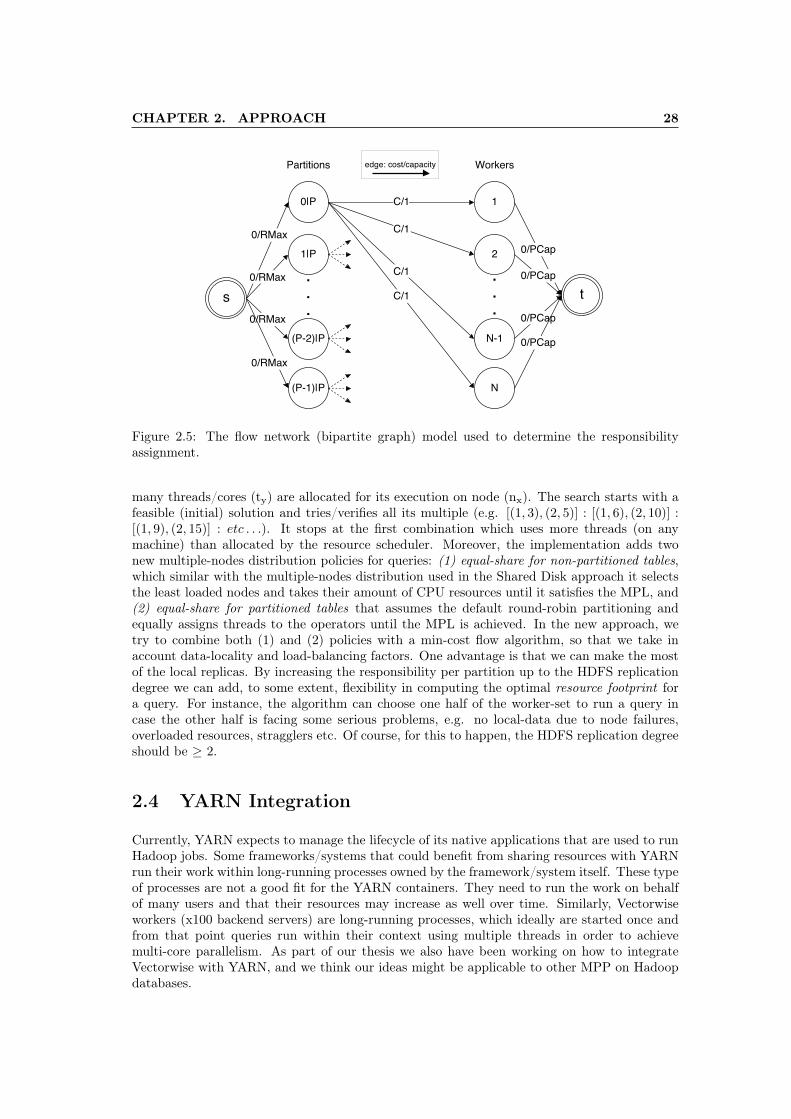
CHAPTER 2. APPROACH 28
Figure 2.5: The flow network (bipartite graph) model used to determine the responsibilityassignment.
many threads/cores (ty) are allocated for its execution on node (nx). The search starts with afeasible (initial) solution and tries/verifies all its multiple (e.g. [(1, 3), (2, 5)] : [(1, 6), (2, 10)] :[(1, 9), (2, 15)] : etc . . .). It stops at the first combination which uses more threads (on anymachine) than allocated by the resource scheduler. Moreover, the implementation adds twonew multiple-nodes distribution policies for queries: (1) equal-share for non-partitioned tables,which similar with the multiple-nodes distribution used in the Shared Disk approach it selectsthe least loaded nodes and takes their amount of CPU resources until it satisfies the MPL, and(2) equal-share for partitioned tables that assumes the default round-robin partitioning andequally assigns threads to the operators until the MPL is achieved. In the new approach, wetry to combine both (1) and (2) policies with a min-cost flow algorithm, so that we take inaccount data-locality and load-balancing factors. One advantage is that we can make the mostof the local replicas. By increasing the responsibility per partition up to the HDFS replicationdegree we can add, to some extent, flexibility in computing the optimal resource footprint fora query. For instance, the algorithm can choose one half of the worker-set to run a query incase the other half is facing some serious problems, e.g. no local-data due to node failures,overloaded resources, stragglers etc. Of course, for this to happen, the HDFS replication degreeshould be ≥ 2.
2.4 YARN Integration
Currently, YARN expects to manage the lifecycle of its native applications that are used to runHadoop jobs. Some frameworks/systems that could benefit from sharing resources with YARNrun their work within long-running processes owned by the framework/system itself. These typeof processes are not a good fit for the YARN containers. They need to run the work on behalfof many users and that their resources may increase as well over time. Similarly, Vectorwiseworkers (x100 backend servers) are long-running processes, which ideally are started once andfrom that point queries run within their context using multiple threads in order to achievemulti-core parallelism. As part of our thesis we also have been working on how to integrateVectorwise with YARN, and we think our ideas might be applicable to other MPP on Hadoopdatabases.

CHAPTER 2. APPROACH 29
There are different ways of integrating long-living application processes within YARN. Usingservice X as an example for the application and queries for the computational-unit, the differentapproaches to integrate service X with YARN can be characterized as follows:
Isolation outside YARN. Carving out part of the cluster nodes for service X and part forYARN (e.g. via Linux CGroups 1 / Linux Container Executor). This is better than just sharingthe same cluster and hoping for no resource contention. This approach is simple and effective,for example, assigning 60% to service X and 40% to YARN. However, it lacks flexibility as loadconditions may change for both sides. Also, it is not possible to assign a common share to auser or a queue across service X and YARN.
Model the service as a YARN application. Implementing service X as a YARN applicationcould be another solution. With this approach, the YARN’s scheduler is responsible for sharingresources among different users and applications. Because service X is a pure YARN application,resources utilization for this service and other YARN applications is dynamically based on theload conditions. A drawback of this approach is that service X will be tightly bound to justone of the scheduler’s queues. While it is possible to run multiple service X instances (multipleYARN applications), one per queue, this may not be practical because the different service Xinstances may have to coordinate among each other and may have to duplicate their resourceheadroom utilization in advance. In addition, as stated in YARN-896 2, there is significant workto be done to allow long live services running as YARN applications. Besides, for the moment, isnot even possible to increase or decrease resource utilization within YARN containers (YARN-1197 3), being impossible "per se" to have some elasticity and to acquire/release resources forservice X when its workload increases/decreases.
Model queries as YARN applications. For this approach we consider that service X residesoutside YARN, having its own resources isolated from YARN, but each of its running queriestranslates into individual YARN applications. Optimizations such as pooling and reusing YARNapplication instances, and the containers within those applications, can help reducing latencysignificantly. An important benefit of this approach is that the resources utilization and dis-tribution is completely managed by YARN. However, this approach assumes that each querysubmitted to service X is a set of independent processes from the service X’s query dispatcher,but in our case all queries run within the Vectorwise worker-set’s processes. Hence, this ap-proach is not an option that could work out and be easily implemented.
Model resource requests as YARN applications. This idea sounds similar with theprevious one, except that now we shift our focus towards requests per workload instead of perquery to decrease the application’s startup latency overhead (in number of requests) and thatservice X is part of the integration too. Making service X use a set of unmanaged YARNApplication Master (more details in Chapter 5) sounds more likely to us. These applicationsare in principle spawned by (1) an initial request for the minimum amount of resources – CPUand memory – needed to bootstrap Vectorwise and be operable to users (e.g. at least 1 core+ enough memory for query execution per node), and (2) extra resource requests to increasethe performance of different query workloads. In this case, service X manages its own processesout-of-band from YARN and only uses the amount of resources allocated by the scheduler. Onthe other hand, the distribution of resources is completely managed by YARN. If service X runsqueries over a set of processes, common resources (i.e. data-structures) can be easily sharedamong different runs without duplication. A drawback of this approach is that service X mustmanage on its own the enforcement of resource utilization per query. Our proposal for theVectorwise-YARN integration fits this approach. However, as YARN-1197 is being pushed forthe next release version, we are going to improve this approach in near future. Hence, instead ofcreating one YARN application per resource request (per workload), we could multiplex all therequests towards a single YARN application (or a pool of applications distributed over different
1Linux CGroups: www.kernel.org/doc/Documentation/cgroups/cgroups.txt2YARN-896: issues.apache.org/jira/browse/YARN-8963YARN-1197: issues.apache.org/jira/browse/YARN-1197

CHAPTER 2. APPROACH 30
scheduling queues) that dynamically increases/decreases the containers’ resource context. Inthis way we can avoid the application startup overhead entirely, reducing the acquire/releaserequest latency even more (i.e. a YARN application can run in background and listen only fornew requests).
Figure 2.6: Out-of-band approach for Vectorwise-YARN integration.
Figure 5.2 depicts our approach for the Vectorwise-YARN integration. As a reminder, in thisapproach we model every resource request (per workload) as a separate YARN application.The integration starts with the Vectorwise worker-set initialization phase. During this phasewe allocate through YARN at least the minimum amount of resources for the database to beoperable, i.e. run distributed queries w/o any parallelism (e.g. 1 core + enough memory forquery execution per node). This phase is managed by the WorkersSetInit component (a customYARN Application Master). From that point on, any needs to increase the worker-set amountof resources, i.e. extra CPU and memory to run a new workload, are translated into message-requests and sent directly to the DbAgent component (a custom YARN Client Application).Besides what is mentioned in Section 2.3, the DbAgent is also responsible for resource allocationwithin YARN, i.e. to release or acquire new containers. What happens under the hood is that,for each request, we spawn a new YARN Application Master (IncreaseResources component)that negotiates with the ResourceManager the demand for extra containers: it reserves andstarts containers with specific resource requirements on a subset of (or all) worker nodes andthen it manages their lifecycle. Previously to any resource request, the Vectorwise Masternode asks the DbAgent for the cluster’s current resource state in order to compute the resourcefootprint of the current query workload. More details about the Vectorwise-YARN integrationare presented in Chapter 5.
CHAPTER 2. APPROACH 31
2.5 Experimentation Platform
All our Linux based cluster nodes granted by Centrum Wiskunde & Informatica 1 (CWI) wereset up using the before-mentioned specifications (e.g. Hadoop v2.2, w/ short-circuit, 128MBHDFS block size, replication degree equal to 3) and served as the experimentation platformfor our prototype during development. For functionality testing and debugging we used thecompany’s internal cluster of 4 nodes, being easier for us to run corner case examples and inves-tigate issues, if any. A brief description of the CWI’s cluster relevant hardware configuration isgiven below.
CWI SciLens cluster
Hardware ("Rocks" nodes)
Nodes: 144 nodes (Shuttle boxes), granted up to 32 nodes
Sockets/CPUs: 1 x Intel Core i7-2600K processor (4 cores, 3.4 GHz, 8 MB cache) per node; 2 threads percore with Hyper-Threading
Memory : 16 GB DDR3 per node
Storage: 1 x 2 TB HDD disks per node (/scratch 1.8 TB partition used for the HDFS data directory)
Disk I/O Throughput Tests (results averaged over 3 runs and rounded up)
dd if=/dev/zero of=out_file bs=1G count=1 oflag=direct : 131 MB/s
dd if=/dev/zero of=out_file bs=1G count=5 oflag=direct : 132 MB/s
Network : 40 Gbit/s InfiniBand interconnection, 1 Gb/s Ethernet
Hardware ("Stones" nodes)
Nodes: 16 nodes (hot-pluggable systems), granted up to 8 nodes
Sockets/CPUs: 2 x Intel Xeon E5-2650 v2 processors (8 cores, 2.6 GHz, 20 MB cache) per node; 2 threadsper core with Hyper-Threading
Memory : 256 GB DDR3 per node
Storage: 3 x 3 TB HDD disks per node w/ software-RAID0 (/scratch 5.4 TB partition used forthe HDFS data directory)
Disk I/O Throughput Tests (results averaged over 3 runs and rounded up)
dd if=/dev/zero of=out_file bs=1G count=1 oflag=direct : 473 MB/s
dd if=/dev/zero of=out_file bs=1G count=5 oflag=direct : 534 MB/s
Network : 40 Gbit/s InfiniBand interconnection, 1 Gb/s Ethernet
Actian internal cluster
Hardware
Nodes: 4 nodes (2 × 2 hot-pluggable nodes in a 2U form-factor)1CWI SciLens cluster: www.monetdb.org/wiki/Main_Page

CHAPTER 2. APPROACH 32
Sockets/CPUs: 2 x Intel Xeon E5645 processors (6 cores, 2.4 GHz, 12 MB cache) per node; Hyper-Threading disabled
Memory : 48 GB DDR3 per node
Storage: 1 x 2 TB HDD (used for the HDFS data directory) disks per node
Disk I/O Throughput Tests - for the HDD disk (results averaged over 3 runs and roundedup)
dd if=/dev/zero of=out_file bs=1G count=1 oflag=direct : 126 MB/s
dd if=/dev/zero of=out_file bs=1G count=5 oflag=direct : 128 MB/s
Network : 40 Gbit/s InfiniBand interconnection, 1 Gb/s Ethernet

Chapter 3
Instrumenting HDFS BlockReplication
This chapter presents in detail the Custom Block Placement Policy for HDFS that we imple-mented in order to control the block (re-)replication and to collocate table partitions to thesame group of DataNodes, therefore achieving data-locality to Vectorwise worker nodes duringfailover situations (e.g. a node fails running our services and it is replaced by a new one).
3.1 Preliminaries
It is sometimes beneficial to have selective overlap among the workers on which the partitionsof two or more tables are stored. If the same hash function and number of partitions arechosen for two (or more) tables, then there will be a one-to-one correspondence between thepartitions of both (or all) tables that will join with one another. If this is the case, then it ispossible to collocate the joining partitions of both (or all) tables. That is, any pair of joiningpartitions will be stored on the same nodes participating in the workers-set. The advantage ofcollocation is that tables can be joined without the need to move any data from one node toanother. However, collocation of joining tables can be nontrivial when there are complex joinrelationships.
Let us consider an example of two tables R and S loaded on a Vectorwise cluster of 3 workers /4 nodes, using a 3-way partitioning and replication degree of 2. Also, assume that both tablesare hash partitioned on the same attribute key and a partition fits in one single HDFS block.An example of a default HDFS block placement, after R and S tables are loaded, is shown inFigure 3.1 - upper image. In this context, consider the following example of a query that joinstables R and S on attribute key :
1 Select *2 From R, S3 Where R.key = S.key
If we assume that nothing happens with the cluster/system (i.e. a node crashes), we can thenprocess parts of the join locally on each node. The default HDFS block replication guaranteesthat it stores the first replica of a block on the node which initiates the write (first-write locality).As for the second replica (or the others, if more) that is not the case. However, only for theirfirst replicas, R’s and S’s partitions are collocated on the same nodes and can be joined locally –R1 can be joined locally with S1 on N1, R2 with S2 on N2 and, respectively, R3 with S3 on N3.Unfortunately, this all changes when a node (or more) fails. All missing block replicas will be
33

CHAPTER 3. INSTRUMENTING HDFS BLOCK REPLICATION 34
discovered and re-replicated (recovery phase) randomly to other nodes within the whole HDFScluster, which can be even larger then the Vectorwise workers-set. If that is the case, we loseour first-write locality and, implicitly, the collocation that is set by the initial bulk load. As aresult, this will make the collocation of joining tables less probable. Considering Figure 3.1 -lower image, to join R3 with S3 on N4 (after re-replication) we would have to access S3 remotelyfrom N1/N2 during the query’s cold-run, or to move this join computation to N2.
Figure 3.1: An example of two tables (R and S) loaded on 3 workers / 4 nodes, using 3-waypartitioning and replication degree of 2: after the initial-load (upper image) vs. during a systemfailover (lower image).
The previous situation becomes even worse if each partition has multiple blocks and/or its (ta-ble) columns are stored in separate HDFS files, as it happens to Vectorwise on Hadoop becauseof the custom columnar HDFS file format. One way to mitigate this problem and achieve fulldata-locality, plus collocation of joining tables, is to properly instrument the HDFS replicationby implementing a custom block placement policy. If tables are partitioned using the samepartitioning-class and on the same attribute or set of attributes, then this policy must collocateand replicate their partitions (their columns and so, implicitly, their HDFS files/blocks) on thesame subset of worker nodes, Section 3.2. A partitioning-class (or partitioning-scheme) is sim-ply the degree of partitioning, i.e. a 3-way partitioning is a partitioning-class. Non-partitionedtables have their partitioning-class too, 1-way partitioning (i.e. 1 single partition). To sum up,one can think of this policy as replicating and collocating Vectorwise column-format HDFS filesinstead of logical partitions.
A formal definition for the custom policy can be stated as: given T tables partitioned on thesame attribute(s), R (degree of replication), P (a partitioning-class) ⇒ ti(pj) ∈ Wj , wherei = 1, . . . , T , j = 1, . . . , P , W = the workers-set, Wj = a subset of our workers-set, |Wj | = R.This definition applies to more than one partitioning-class. We note that two or more replicasof the same HDFS block cannot be stored on the same node.
Going back to our previous example, now R’s and S’s partitions can be replicated and collocatedon the same subset of worker nodes: R1 with S1, R2 with S2 and R3 with S3, on {N1, N2},{N2, N3} and, respectively, {N3, N1}. A general illustration of what can we achieve with a3-way partitioning on 3 workers / 4 nodes is depicted in Figure 3.2.

CHAPTER 3. INSTRUMENTING HDFS BLOCK REPLICATION 35
Figure 3.2: Instrumenting the HDFS block replication, in three scenarios, to maintain block(co-)locality to worker nodes.
3.2 Custom HDFS Block Placement Implementation
We have enhanced the default HDFS block replication and implemented a custom block place-ment policy (only) for Vectorwise partitioned tables. Other HDFS (non-Vectorwise) files arenot considered by our replication policy, since we filter Vectorwise files by their naming pattern<table-name>@<partition-ID>, where <partition-ID> is <partition-number>c<partitioning-class>. The custom policy makes sure that the HDFS blocks of all files with the same partition-id (implicitly all columns of a table) and their replicas are collocated on exact R target nodes(R equal to the replication degree). We specify the exact R nodes in a global location-map.This particular data structure is generated at startup by the DbAgent component and thensaved at the Vectorwise HDFS database location into a metadata file – called plocations. Theend result is that multiple Vectorwise column-format HDFS files are collocated on the same setof nodes and that (re-)replication (the recovery phase) is now under the control of the globallocation-map whenever nodes might fail.
An example of a plocations file (or global location map), in Json format, for 3 nodes, replicationdegree 2, and 3 (1-, 3-, 6-) partitioning-classes is:
1 { // plocations metadata file in Json format: <partition-ID>:[<location>,...]2 // we assign a list of locations (worker nodes) to every <partition-ID>3 "0c1":["node1","node2"],"0c3":["node1","node2"],"1c3":["node2","node3"],4 "2c3":["node3","node1"],"0c6":["node1","node2"],"1c6":["node2","node3"],5 "2c6":["node3","node1"],"3c6":["node1","node2"],"4c6":["node2","node3"],6 "5c6":["node3","node1"] }
CHAPTER 3. INSTRUMENTING HDFS BLOCK REPLICATION 36
3.2.1 Adding (New) Metadata to Database Locations
The plocations file is stored only once at the Vectorwise database location, since we can easilyshare this path with our DbAgent at startup time. All metadata files that theDbAgent generatesare stored there. Moreover, whenever a (Vectorwise columnar-) file is being written to HDFSblock by block, the only information we are provided by the API is its full source path. So,though we can extract and parse from a Vectorwise file’s path its exact table location, simply,from the Block Placement Policy class, we cannot determine to which database location itbelongs to (not without extra communication with the Vectorwise Master node). This meansthat the global location-map is not (directly) visible to other table locations, including thedefault one. Nevertheless, this information is still needed to select the target (worker-) nodesfor block replication. It is clear by now that what we need is a way to refer to the databaselocation from any table location. An easy way to do so is to keep the default database location(the HDFS path) into a metadata file, and, whenever a table location is created (including thedefault one), have it stored directly within that path.
3.2.2 Extending the Default Policy
To implement our Vectorwise custom block placement policy, we used the HDFS-385 1 feature,which is already part of HDFS since the 0.21 release. This improvement provides a way forthe developer to write Java code, within the same HDFS namespace, that can instrument theblock replication and specify, directly for instance, what target nodes should be used to storeone file’s blocks including their replicas. The default behavior of the block placement policycan be modified by extending the BlockPlacementPolicy abstract class 2.
Another way is to overload some of the BlockPlacementPolicyDefault’s class 3 methods, like wedid in order to maintain/keep the default block replication for the rest of the (non-Vectorwisecustom format) HDFS files. More specifically, what we did was to overload the chooseTargetN-odes(...) method and diverge the default work-flow for Vectorwise data. Whenever an HDFSblock of a Vectorwise column-file is being stored and the latter method is called, we use our ownchoose target nodes method instead – named chooseVWTargetNodes(...) – to compute (andreturn) the list of datanode descriptors for block replication.
Algorithm 3.3 contains the pseudo-code for chooseVWTargetNodes(...) method, referred pre-viously. First, at lines 1 to 3 we read the (static) configuration values for global location-mapfile’s name, table’s location metadata file’s name and the Vectorwise HDFS file pattern. In steps6-8 we extract from the block’s source path its directory path, the name of the file which belongsto, and the table’s partition-ID. Then, at line 9 we cache the global location-map for the currentdatabase location. Line 12 determines the available (alive) target nodes for block replicationusing the (in-memory cached) global location-map. The target nodes are mapped by the table’spartition-ID. From 13 to 22 we check if there are stale entries in cache and, if any, we re-cacheall entries by reading again the global location-map metadata from its source file. Finally, lines23 to 34 fills out the results list with target descriptors and returns the writer descriptor. Itconverts the available target nodes (hostnames) into a datanode descriptors list. Then, it usesthis list to merge with results and to determine the writer descriptor.
Both algorithms, Algorithm 3.1 and Algorithm 3.2, come to help in Algorithm 3.3 when cachingis needed for the global location-map. By this, we omit multiple metadata file reads that candegrade our performance. Reading once and then saving the metadata in (NameNode’s) mem-ory makes it fast enough to retrieve the right target nodes during the HDFS block replication.
1HDFS-385: issues.apache.org/jira/browse/HDFS-3852BlockPlacementPolicy abstract class: grepcode.com/file/repo1.maven.org/maven2/org.apache.hadoop/hadoop-
hdfs/0.22.0/org/apache/hadoop/hdfs/server/namenode/BlockPlacementPolicy.java3BlockPlacementPolicyDefault class: grepcode.com/file/repo1.maven.org/maven2/org.apache.hadoop/hadoop-
hdfs/2.2.0/org/apache/hadoop/hdfs/server/blockmanagement/BlockPlacementPolicyDefault.java

CHAPTER 3. INSTRUMENTING HDFS BLOCK REPLICATION 37
However, when the cache contains stale entries (i.e. due to node failures), we do have to discardthe data by (re-)reading again the (possible new) file’s content.
Algorithm 3.1 Cache the table’s location metadata file:cacheTableLocMetadata(tableLocation, tableLocFilename)
Input: tableLocation: the HDFS path towards the table location, tableLocFilename: the table’slocation metadata filename (default is .metadata)
1: if ¬dbLocationsMap.containsKey(tableLocation) then // synchronized section2: tableLocMetadataPath← makePath(tableLocation, tableLocF ilename)3: dbLocation← readDbLocMetadata(tableLocMetadataPath) // read HDFS path, one liner4: if dbLocation = ∅ then // invalid path or the file is empty5: throw error6: end if7: dbLocationsMap.putEntry(tableLocation, dbLocation)8: end if
The first algorithm, Algorithm 3.1, uses a concurrent hash map to store table locations todatabase location many-to-1 relations, where the database location (HDFS path) is read from thetable’s location metadata file. The second one, Algorithm 3.2, uses a concurrent hash map datastructure too, but to store 1:1 relations between a database location and its plocations metadatafile (the global location-map generated each time by the DbAgent during the Vectorwise clusterstartup).
Algorithm 3.2 Cache the global location-map file:cachePLocations(tableLocation, tableLocFilename, pLocFilename)
Input: tableLocation: the path towards the HDFS table location, tableLocFilename: the table’slocation metadata filename (default is .metadata), pLocFilename: the global location-mapmetadata filename (default is plocations), one per Vectorwise database location
1: cacheTableLocMetadata(tableLocation, tableLocF ilename) // we make sure to cache the table’slocation metadata beforehand
2: dbLocation← dbLocationsMap.getV alue(tableLocation)3: if dbLocation does not exist anymore in HDFS then // stale entry4: // remove the correspondent metadata entries from dbLocationsMap and pLocationsMap
5: dbLocationsMap.removeEntry(tableLocation)6: pLocationsMap.removeEntry(dbLocation)7: cacheTableLocMetadata(tableLocation, tableLocF ilename) // and re-cache8: dbLocation← dbLocationsMap.getV alue(tableLocation)9: end if
10: if ¬pLocationsMap.containsKey(dbLocation) then // synchronized section11: pLocationsPath← makePath(dbLocation, pLocF ilename)12: pLocations ← readPLocMetadata(pLocationsPath) // read the global location-map for the
current database session13: if pLocations = ∅ then // invalid path or the file is empty14: throw error15: end if16: pLocationsMap.putEntry(dbLocation, pLocations)17: end if
Besides Algorithm 3.3, we have also extended/overloaded the HDFS file-system-check primitives(not shown) to ease-up the system administration routines, i.e. a sysadmin can check if thenode locations of Vectorwise HDFS blocks are consistent with the global location-map and ifnot, those blocks will be automatically moved to their right destination.

CHAPTER 3. INSTRUMENTING HDFS BLOCK REPLICATION 38
Algorithm 3.3 Choose the Vectorwise target (worker-) nodes for block replication:chooseVWTargetNodes(blockSrcPath, numOfReplicas, writer, results)
Input: blockSrcPath: the full source path of the HDFS block being written, numOfReplicas:number of replicas needed, writer: the datanode’s descriptor that initiates the write oper-ation, results: the list of chosen target nodes (datanode descriptors) for block replication –for a new block this list is empty, whereas for an old block with missing replicas it containsthe rest of the nodes (datanode descriptors) where that block is stored
Output: the datanode descriptor for the first-write locality and, indirectly, the target nodes(the descriptors results list)
1: pLocF ilename← configPropertyGet(ploc_metadata_property)2: tableLocF ilename← configPropertyGet(tableloc_metadata_property)3: pattern← configPropertyGet(vwfile_pattern_property)4: newBlock ← (results.size = 0) // true if is empty, false otherwise5: totalReplicas← numOfReplicas+ results.size6: srcDirname← extractDirname(blockSrcPath)7: srcF ilename← extractF ilename(blockSrcPath)8: pId← extractPartitonId(blockSrcPath, pattern)9: cachePLocations(srcDirname, tableLocF ilename, pLocF ilename)
10: dbLocation← dbLocationsMap.get(srcDirname)11: pLocations← pLocationsMap.get(dbLocation)12: targetNodes← getAvailableTargetNodes(pLocations, pId)13: if targetNodes.size < totalReplicas then // stale metadata14: // remove the correspondent plocations entry from plocationsMap
15: pLocationsMap.removeEntry(dbLocation)16: cachePLocations(srcDirname, tableLocF ilename, pLocF ilename) // and re-cache17: pLocations← pLocationsMap.get(dbLocation)18: targetNodes← getAvailableTargetNodes(pLocations, pId)19: if targetNodes.size < totalReplicas then // still stale, DbAgent was not yet restarted20: fill-out targetNodes with nodes from the remaining Vectorwise cluster (use the least-
loaded nodes)21: end if22: end if23: targetDesc← toDataNodeDescriptors(targetNodes)24: if newBlock = true then25: if writer = null ∨ ¬targetDesc.contains(writer) then26: writer ← targetDesc[0]27: end if28: results.add(writer) // the local descriptor has to be the first29: merge results with targetDesc, maximum numOfReplicas30: return writer31: end if32: // an old block33: merge results with targetDesc, maximum numOfReplicas // fill-out missing replicas34: return writer
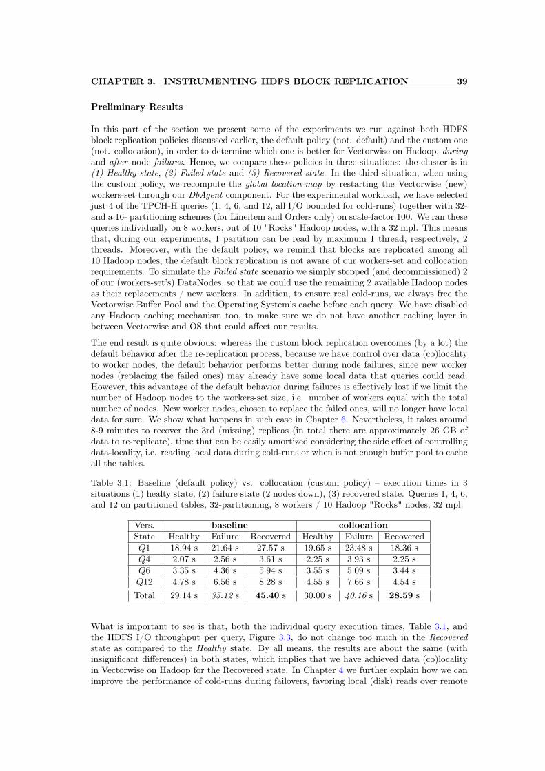
CHAPTER 3. INSTRUMENTING HDFS BLOCK REPLICATION 39
Preliminary Results
In this part of the section we present some of the experiments we run against both HDFSblock replication policies discussed earlier, the default policy (not. default) and the custom one(not. collocation), in order to determine which one is better for Vectorwise on Hadoop, duringand after node failures. Hence, we compare these policies in three situations: the cluster is in(1) Healthy state, (2) Failed state and (3) Recovered state. In the third situation, when usingthe custom policy, we recompute the global location-map by restarting the Vectorwise (new)workers-set through our DbAgent component. For the experimental workload, we have selectedjust 4 of the TPCH-H queries (1, 4, 6, and 12, all I/O bounded for cold-runs) together with 32-and a 16- partitioning schemes (for Lineitem and Orders only) on scale-factor 100. We ran thesequeries individually on 8 workers, out of 10 "Rocks" Hadoop nodes, with a 32 mpl. This meansthat, during our experiments, 1 partition can be read by maximum 1 thread, respectively, 2threads. Moreover, with the default policy, we remind that blocks are replicated among all10 Hadoop nodes; the default block replication is not aware of our workers-set and collocationrequirements. To simulate the Failed state scenario we simply stopped (and decommissioned) 2of our (workers-set’s) DataNodes, so that we could use the remaining 2 available Hadoop nodesas their replacements / new workers. In addition, to ensure real cold-runs, we always free theVectorwise Buffer Pool and the Operating System’s cache before each query. We have disabledany Hadoop caching mechanism too, to make sure we do not have another caching layer inbetween Vectorwise and OS that could affect our results.
The end result is quite obvious: whereas the custom block replication overcomes (by a lot) thedefault behavior after the re-replication process, because we have control over data (co)localityto worker nodes, the default behavior performs better during node failures, since new workernodes (replacing the failed ones) may already have some local data that queries could read.However, this advantage of the default behavior during failures is effectively lost if we limit thenumber of Hadoop nodes to the workers-set size, i.e. number of workers equal with the totalnumber of nodes. New worker nodes, chosen to replace the failed ones, will no longer have localdata for sure. We show what happens in such case in Chapter 6. Nevertheless, it takes around8-9 minutes to recover the 3rd (missing) replicas (in total there are approximately 26 GB ofdata to re-replicate), time that can be easily amortized considering the side effect of controllingdata-locality, i.e. reading local data during cold-runs or when is not enough buffer pool to cacheall the tables.
Table 3.1: Baseline (default policy) vs. collocation (custom policy) – execution times in 3situations (1) healty state, (2) failure state (2 nodes down), (3) recovered state. Queries 1, 4, 6,and 12 on partitioned tables, 32-partitioning, 8 workers / 10 Hadoop "Rocks" nodes, 32 mpl.
Vers. baseline collocationState Healthy Failure Recovered Healthy Failure RecoveredQ1 18.94 s 21.64 s 27.57 s 19.65 s 23.48 s 18.36 sQ4 2.07 s 2.56 s 3.61 s 2.25 s 3.93 s 2.25 sQ6 3.35 s 4.36 s 5.94 s 3.55 s 5.09 s 3.44 sQ12 4.78 s 6.56 s 8.28 s 4.55 s 7.66 s 4.54 sTotal 29.14 s 35.12 s 45.40 s 30.00 s 40.16 s 28.59 s
What is important to see is that, both the individual query execution times, Table 3.1, andthe HDFS I/O throughput per query, Figure 3.3, do not change too much in the Recoveredstate as compared to the Healthy state. By all means, the results are about the same (withinsignificant differences) in both states, which implies that we have achieved data (co)localityin Vectorwise on Hadoop for the Recovered state. In Chapter 4 we further explain how we canimprove the performance of cold-runs during failovers, favoring local (disk) reads over remote
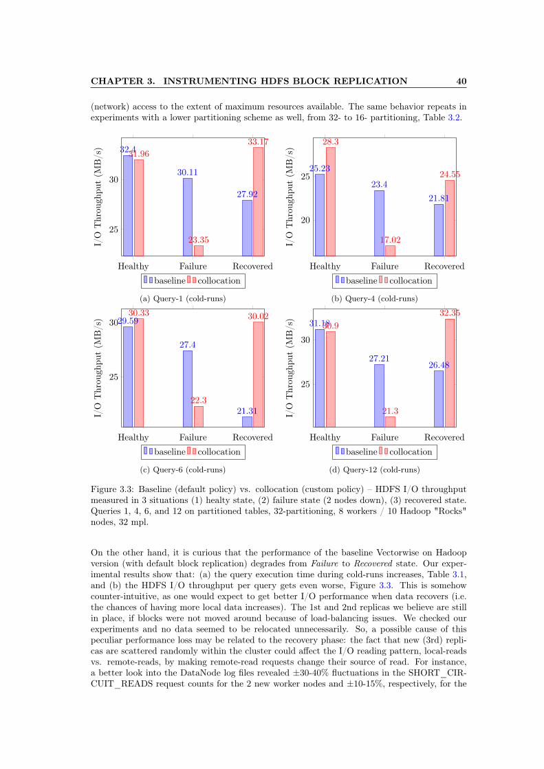
CHAPTER 3. INSTRUMENTING HDFS BLOCK REPLICATION 40
(network) access to the extent of maximum resources available. The same behavior repeats inexperiments with a lower partitioning scheme as well, from 32- to 16- partitioning, Table 3.2.
Healthy Failure Recovered
25
30
32.4
30.11
27.92
31.96
23.35
33.17
I/O
Throu
ghpu
t(M
B/s)
baseline collocation
(a) Query-1 (cold-runs)
Healthy Failure Recovered
20
2525.23
23.4
21.81
28.3
17.02
24.55
I/O
Throu
ghpu
t(M
B/s)
baseline collocation
(b) Query-4 (cold-runs)
Healthy Failure Recovered
25
3029.59
27.4
21.31
30.33
22.3
30.02
I/O
Throu
ghpu
t(M
B/s)
baseline collocation
(c) Query-6 (cold-runs)
Healthy Failure Recovered
25
30
31.18
27.2126.48
30.9
21.3
32.35
I/O
Throu
ghpu
t(M
B/s)
baseline collocation
(d) Query-12 (cold-runs)
Figure 3.3: Baseline (default policy) vs. collocation (custom policy) – HDFS I/O throughputmeasured in 3 situations (1) healty state, (2) failure state (2 nodes down), (3) recovered state.Queries 1, 4, 6, and 12 on partitioned tables, 32-partitioning, 8 workers / 10 Hadoop "Rocks"nodes, 32 mpl.
On the other hand, it is curious that the performance of the baseline Vectorwise on Hadoopversion (with default block replication) degrades from Failure to Recovered state. Our exper-imental results show that: (a) the query execution time during cold-runs increases, Table 3.1,and (b) the HDFS I/O throughput per query gets even worse, Figure 3.3. This is somehowcounter-intuitive, as one would expect to get better I/O performance when data recovers (i.e.the chances of having more local data increases). The 1st and 2nd replicas we believe are stillin place, if blocks were not moved around because of load-balancing issues. We checked ourexperiments and no data seemed to be relocated unnecessarily. So, a possible cause of thispeculiar performance loss may be related to the recovery phase: the fact that new (3rd) repli-cas are scattered randomly within the cluster could affect the I/O reading pattern, local-readsvs. remote-reads, by making remote-read requests change their source of read. For instance,a better look into the DataNode log files revealed ±30-40% fluctuations in the SHORT_CIR-CUIT_READS request counts for the 2 new worker nodes and ±10-15%, respectively, for the

CHAPTER 3. INSTRUMENTING HDFS BLOCK REPLICATION 41
other nodes. The same behavior repeats with 16- partitioning, Table 3.2, but, interestinglythough, not if we restrain the number of Hadoop nodes to the workers-set size (as shown inChapter 6).
Table 3.2: Baseline (default policy) vs. collocation (custom policy) – execution times in 3situations (1) healty state, (2) failure state (2 nodes down), (3) recovered state. Queries 1, 4, 6and 12 on partitioned tables, 16-partitioning, 8 workers / 10 Hadoop "Rocks" nodes, 32 mpl.
Vers. baseline collocationState Healthy Failure Recovered Healthy Failure RecoveredQ1 17.64 s 19.37 s 27.65 s 17.29 s 29.34 s 17.78 sQ4 1.52 s 2.43 s 3.33 s 1.37 s 2.58 s 1.30 sQ6 3.00 s 4.02 s 6.92 s 3.21 s 5.53 s 3.04 sQ12 4.72 s 6.12 s 7.85 s 3.90 s 7.85 s 3.47 sTotal 26.88 s 31.94 s 45.75 s 25.77 s 45.30 s 25.59 s
Conclusion
We have presented in detail our Custom Block Placement Policy for HDFS, designed to controlthe HDFS block (re-)replication and to collocate (Vectorwise) table partitions to the samegroup of DataNodes (specified via plocations metadata file). The preliminary results fromTables 3.1 and 3.2 prove that we can still achieve data-locality to Vectorwise worker nodesduring failover situations (e.g. a node fails running our services and it is replaced by a newone). However, as Chapter 6 shows, there is yet some room left for improving the latter byfavoring local reads over remote (over-the-network) reads.

Chapter 4
Dynamic Resource Management
This chapter describes the steps towards enabling dynamic resource management in Vectorwiseon Hadoop. Our approach is threefold:
1. we first have to determine the Vectorwise worker-set (Section 4.1),
2. then assign (partition) responsibilities to these workers (Section 4.2)
3. and finally, schedule the cluster resources that a query can use at runtime by computingan optimal resource footprint, what particular nodes and the amount of resources, suchas CPU and memory, to use (Section 4.3).
4.1 Worker-set Selection
Currently in Vectorwise on Hadoop, to start a database cluster session, human intervention isneeded to explicitly specify the list of worker nodes as an argument to the Vectorwise clustermpi_run command. An automatic approach for the worker-set selection is yet to be done. Oneway of doing this automatically in Vectorwise on Hadoop is to enhance the Ingres client with theability to query YARN (Resource Manager) and discover which nodes are alive in the cluster,plus what are their resource specifications. Once it determines the best N nodes from all M (≥N) Vectorwise cluster nodes, with respect to their data-locality and resource capabilities, theIngres client can then start the X100 worker-set through the mpi_fork command. All that asysadmin has to do is to write down the list of Vectorwise (on Hadoop) cluster nodes, the Mhostnames that have the X100 server binaries already deployed, in the configuration file.
However, the Ingres client can be configured and used on any remote host-machine outside theHadoop cluster. That makes it difficult to manage a Vectorwise (X100) worker-set from thefrontend itself. We could probably use YARN’s and HDFS’s REST APIs to perform the threesteps enumerated in the beginning of this chapter, but for more complex management tasks,for instance allocate or release cluster resources within YARN, scan HDFS for data, file systemcheck, etc., we must run within the Hadoop environment and implement its native Java APIs.Due to this constraint, we have decoupled the Vectorwise start/stop database functionality fromIngres, implemented with the mpi_fork command, and replaced it with a separate client-servercommunication. Whereas the server is a new Java component that runs in the Hadoop environ-ment (the DbAgent component) and takes care of the worker-set selection, starting/stoppingthe X100 workers, responsibility assignment and Vectorwise-YARN integration for resourcemanagement, the client (the VectorwiseLauncher component, written in Java too) runs on theIngres side and forwards the start/stop database commands as (TCP/IP) message requests tothe agent, along with the list of parameters needed to initialize the X100 backend processes.
42

CHAPTER 4. DYNAMIC RESOURCE MANAGEMENT 43
Upon receiving a start request, the DbAgent determines the worker nodes and then spawnstheir X100 processes using the same mpi_fork command. The VectorwiseLauncher connectionto DbAgent is kept alive during the entire database session and it can be stopped from bothsides, either (1) from the (DbAgent) server side, signifying that there was an issue with runningthe cluster, or (2) from the (VectorwiseLauncher) client side if the user decides to do so. Thewhole process of starting the worker-set through the DbAgent component is depicted in Fig-ure 4.1. No changes were done to the (Ingres to X100 session-master) communication protocolthat provides Vectorwise with an optimal query execution plan and then returns back the finalresult to the user.
Figure 4.1: Starting the Vectorwise on Hadoop worker-set through VectorwiseLauncher andDbAgent. All related concepts to this section are emphasized with a bold black color.
The general idea for the worker-set selection is to first sort out all M Vectorwise (Hadoop)cluster nodes in descending order by their local data size (i.e. existent Vectorwise columnarHDFS local files) and resource (e.g. CPU, memory, etc) capabilities, then choose the top N (≤M) nodes. This twofold process is handled transparently by the DbAgent, using the Hadoop(YARN and HDFS) native Java APIs:
Get the HDFS block locations. To find out where (on which Hadoop nodes) the Vector-wise data is located, the DbAgent component queries the HDFS Namenode for the location-information of all files stored at any of the Vectorwise table locations (HDFS paths) and ofwhich names comply with the table-name@partition-ID pattern (see Section 3.2). The tables’locations are read from the Vectorwise location-map metadata file, found at the database lo-cation path. For each location-information entry we get the file’s size, the list of block IDscomposing the file, plus the node locations of all its R block copies, where R is the HDFSreplication degree. Assuming that our custom HDFS block replication is enabled and that Vec-torwise data was bulk-loaded into the system beforehand, every block from the list must havethe same R node locations. This implies that we just need the first block from it in order todetermine the file’s R node locations, making the HDFS data scan faster.
Sort nodes by resource capabilities. In order to get the resource capabilities of Vectorwisenodes, the DbAgent first asks YARN (Resource Manager) for the list of all cluster node reports.A node report contains an updated summary of runtime information. It includes details suchas the ID of the node, HTTP tracking URL, rack name, used resources, total resources, andthe number of running containers on the node. An example of a Json-format response for nodereports, using an API call with a similar functionality (but from YARN’s REST API), is:

CHAPTER 4. DYNAMIC RESOURCE MANAGEMENT 44
1 { // Cluster Nodes API2 // JSON response from the HTTP Request:3 // GET http://<Resource-Manager-http-address:port>/ws/v1/cluster/nodes4 "nodes":{5 "node":[6 {7 "rack":"default-rack",8 "state":"NEW",9 "id":"node2:1235",
10 "nodeHostName":"node2",11 "nodeHTTPAddress":"node2:2",12 "healthStatus":"Healthy",13 "lastHealthUpdate":1324056895432,14 "healthReport":"Healthy",15 "numContainers":0,16 "usedMemoryMB":017 "totalMemoryMB":8192,18 "usedVirtualCores":0,19 "totalVirtualCores":820 },21 {22 "rack":"default-rack",23 "state":"RUNNING",24 "id":"node1:1234",25 "nodeHostName":"node1",26 "nodeHTTPAddress":"node1:2",27 "healthStatus":"Healthy",28 "lastHealthUpdate":1324056895092,29 "healthReport":"Healthy",30 "numContainers":0,31 "usedMemoryMB":4096,32 "totalMemoryMB:8129,33 "usedVirtualCores":434 "totalVirtualCores":8,35 }36 ]37 }38 }
From the entire list of Hadoop node reports we then filter out those that are not for Vectorwisenodes (based on the list of nodes provided in the configuration file) and their state informationis not set to running. From the report itself we find the total/used amount of memory andthe total/used number of virtual-cores as the only information useful to us, from which we canderive the current available memory and virtual-cores. Using these metrics we can build ourown internal node reports list and sort it in decreasing order (by "totals") to get the top mostresourceful Vectorwise cluster nodes. That aside, an important aspect which matters for theworker-set selection and should be added to the sorting criterias, is the size of Vectorwise localblock data. Since our custom block replication policy tries to limit the replication domain justto the worker-set, a node that has more local data than another will have bigger chances to holdmore table-partitions. To sum up, this approach would help us to determine the appropriateVectorwise worker-set which has all of our data and its worker nodes are among the cluster’sbest nodes.
Based on the data-locality information obtained during the HDFS file system scan, we candetermine the missing replicas (i.e. in case of node failures) from the system and start re-replicating them to (possibly new) other workers. Also, we can automatically increase anddecrease the worker-set at startup time and re-arrange the Vectorwise partitions to a newconfiguration of worker nodes. The problem of (re-)balancing data to worker nodes and creatingthe global location-map can be formulated as a min-cost matching problem on a bipartite graphwhere the cost model reflects the Vectorwise data-locality to worker nodes. For the initialbulk-load we use a round-robin (horizontally) data partitioning scheme, Algorithm 4.1.
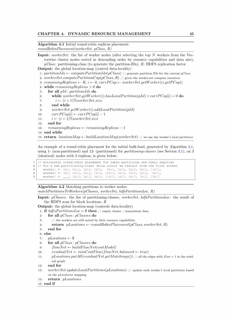
CHAPTER 4. DYNAMIC RESOURCE MANAGEMENT 45
Algorithm 4.1 Initial round-robin replicas placement:roundRobinPlacement(workerSet, pClass, R)
Input: workerSet: the list of worker nodes (after selecting the top N workers from the Vec-torwise cluster nodes sorted in descending order by resource capabilities and data size),pClass: partitioning-class (to generate the partition-IDs), R: HDFS replication factor
Output: the global location-map (control data-locality)1: partitionIds← computePartitionIds(pClass) // generate partition IDs for the current pClass
2: workerSet.computePartitionCap(pClass,R) // given the worker-set compute resources3: remainingReplicas← R, i← 0, currPCap← workerSet.getWorker(i).getPCap()4: while remainingReplicas > 0 do5: for all pId : partitionIds do6: while workerSet.getWorker(i).hasLocalPartition(pId) ∨ currPCap[i] = 0 do7: i← (i+ 1)%workerSet.size8: end while9: workerSet.getWorker(i).addLocalPartition(pId)
10: currPCap[i]← currPCap[i]− 111: i← (i+ 1)%workerSet.size12: end for13: remainingReplicas← remainingReplicas− 114: end while15: return locationMap← buildLocationMap(workerSet) // we use the worker’s local partitions
An example of a round-robin placement for the initial bulk-load, generated by Algorithm 4.1,using 1- (non-partitioned) and 12- (partitioned) for partitioning-classes (see Section 3.1), on 3(identical) nodes with 2 replicas, is given below:
1 // Horizontal round-robin placement for table partitions and their replicas2 // For a new partitioning-class (blue color) we restart from the first worker3 worker1 <- 0c1, 0c12, 3c12, 6c12, 9c12, 2c12, 5c12, 8c12, 11c12,4 worker2 <- 0c1, 1c12, 4c12, 7c12, 10c12, 0c12, 3c12, 6c12, 9c12,5 worker3 <- ___, 2c12, 5c12, 8c12, 11c12, 1c12, 4c12, 7c12, 10c12
Algorithm 4.2 Matching partitions to worker nodes:matchPartitionsToWorkers(pClasses, workerSet, hdfsPartitionsLoc, R)
Input: pClasses: the list of partitioning-classes, workerSet, hdfsPartitionsLoc: the result ofthe HDFS scan for block locations, R
Output: the global location-map (controls data-locality)1: if hdfsPartitionsLoc = ∅ then // empty cluster / nonexistent data2: for all pClass : pClasses do3: // the workers are still sorted by their resource capabilities4: return pLocations← roundRobinP lacement(pClass, workerSet,R)5: end for6: else7: pLocations← ∅8: for all pClass : pClasses do9: flowNet← buildF lowNet(costModel)
10: residualNet← minCostF low(flowNet, balanced← true)11: pLocations.putAll(residualNet.getMatchings()) // all the edges with flow = 1 in the resid-
ual graph12: end for13: workerSet.updateLocalPartitions(pLocations) // update each worker’s local partitions based
on the pLocations mapping14: return pLocations15: end if

CHAPTER 4. DYNAMIC RESOURCE MANAGEMENT 46
However, following the initial bulk-load, the global location-map (plocations metadata) willalways be re-generated according to the current location of the Vectorwise partitions (i.e. thecolumnar HDFS files including their replicas) at startup time, Algorithm 4.2. Before digginginto this algorithm’s pseudo-code, we recommend reading the cost model description in the nextparagraphs.
When both (1) querying HDFS for Vectorwise block locations and (2) sorting Hadoop nodesby resource capabilities steps are done, we can compute the cost model and generate the flownetwork for the the matching algorithm, the annotated bipartite graph from Figure 4.2. Findingan optimal matching in a bipartite-graph is a min-cost flow sub-problem which can be solvedwith the Successive Shortest Path algorithm [49]. We explain the algorithm’s implementation(and our own changes to it) in the last section of this chapter. As for the current and nextsection we briefly explain the (bipartite graphs) cost models and the pseudo-code of the mainfunctions, more specifically Algorithm 4.2 and 4.3, from which the min-cost flow algorithm isbeing called.
Figure 4.2: The flow network (bipartite graph) model used to match partitions to worker nodes.
Cost model. The bipartite-graph from Figure 4.2 is structured as follows: (1) left-side :partition-IDs and (2) right-side : workers (the whole worker-set). What exactly is a partition-IDwe can remember from Section 3.2. From our source (s) to each partition-ID, we connect edgeswith cost 0 and capacity equal to the HDFS replication degree (R). Then, from a partition-IDto a worker we use the capacity 1 and cost 0 for local partitions, or cost 1 for non-local/remotepartitions. To determine whether a partition is physically stored or not on a particular clusternode, we simply use the HDFS results from the previous file system scan. Finally, we link ourworkers to their destination node (t). We assign these edges a cost 0 and a capacity equal to thepartition-capacity (PCap) of that worker node. The end result is a load-balanced mapping frompartitions to nodes; it actually represents the global location-map to which we referred manytimes in previous paragraphs. Already mentioned, this mapping is used mostly during the (1)custom HDFS block replication (Section 3.2) and (2) responsibility assignment (Section 4.2),and it is materialized into the plocations metadata file that is found at the Vectorwise databaselocation path.
CHAPTER 4. DYNAMIC RESOURCE MANAGEMENT 47
With each node’s PCap (partition-capacity) we can restrict the edge capacities in the cost modelwith respect to heterogeneous cluster configurations, although all recent Hadoop implementa-tions assume all nodes in the cluster to be homogeneous in nature. We know from [50] thatHadoop is lacking performance in an environment with different hardware specs and therefore,in practice, all cluster nodes should roughly have the same computing capacity. If not, this caneffect MPP database systems, which usually prefer an equipartition strategy to load-balancedata for effective resource utilization. The latter has bee proven to be an efficient strategyin general [13, 14, 42]. Nevertheless, Vectorwise on Hadoop uses its own worker-set selectionstrategy (see Section 1.3.3), in which Hadoop nodes with similar resource capabilities are chosento run the X100 backend processes.
The PCapi partition-capacity (or the maximum partition load) determines how many partitions(plus R replicas) matching with any of the partition-IDs (left side) can be assigned to a workernode (right side), considering the number of cores and amount of memory, while running (min-cost flow) algorithm. It simply acts as an arc capacity in the bipartite-graph. On the one hand,this is quite relevant for computing the cost model in order to (re-)balance the Vectorwise tablepartitions (with partition-IDs in left-side) to the worker-set (on right side), but also for theround-robin placement we perform before the initial data bulk-load. The worker’s partition-capacity has the following formula:
PCapi = d(Ci ∗ PRatioi) ∗ Mi
MAvg e,PRatioi =
PTot−PCapi−1
CTot−Ci−1,
i = 1, . . . , N , PCap0 = 0 and C0 = 0
where:
• N is the worker-set size,
• Ci and Mi are the number of cores, respectively, the memory size of workeri,
• PRatio is the partitions-per-core ratio (computed iteratively),
PTot = P ∗R is the total number of partitions (including their R replicas),
CTot is the worker-set total number of cores (aggregated number),
• MAvg = MTotN is the worker-set average amount of memory,
MTot is the the worker-set total amount of memory (aggregated number)
The reason why the above formula refers to one partitioning-class (see Section 3.2) is that wecompute the cost model and run the matching algorithm iteratively for each class. This givesus a much better load-balancing per node since the matching (implicitly the min-cost flow)algorithm, by itself, cannot distinguish between different partitioning-classes. Otherwise, wemight end up with all the partitions from the same partitioning-class stored on one single node.Obviously, such a result is not load-balanced, i.e. different partitioning-classes implies differentpartition sizes. We note the reader that we will continue referring to one partitioning-class inthe following paragraphs for simplicity reasons, though in our implementation all the algorithmsand cost models are applied individually to each of these classes.
4.2 Responsibility Assignment
There are multiple ways to assign partition responsibilities to worker nodes. We have intro-duced the meaning of partition responsibilities and responsibility assignment in Section 1.3.3.These concepts are emphasized in Figure 4.3. Depending on the HDFS replication degree, theresponsibility assignment can vary from one-to-one assignment with one node being respon-sible per partition, to many-to-one assignments where two or more nodes may be responsible

CHAPTER 4. DYNAMIC RESOURCE MANAGEMENT 48
for the same partition. As we pointed in Section 4.1, the location-map metadata returned bythe previous Algorithm 4.2 is one of the input data to find the responsibility assignment, aswill see in Algorithm 4.3. Even though both algorithms use the same approach (i.e. finding amin-cost flow) to solve the matching problem in bipartite graphs, the difference is in the costmodel. What is important to know is that we have now extended the cost model to take inaccount local partitions that were assigned last time already and so, they may have been cachedby the worker’s OS while doing I/O for Vectorwise queries.
Figure 4.3: Assigning responsibilities to worker nodes. All related concepts to this section areemphasized with bold black and red/blue/green colors (for single (partition) responsibilities).
Cost model. To assign responsibilities to worker nodes we run the min-cost flow algorithmfor the bipartite graph that is illustrated in Figure 4.4. Likewise the previous bipartite graph,this one is structured in (1) left-side : partition-IDs and (2) right-side : workers as well. Fromthe source (s) to each partition vertex, we connect edges with cost 0 and capacity equal to theresponsibility degree, annotated in the figure with RMax. For a one-to-one assignment, withmaximum one node being responsible per partition, RMax is set to 1. When two or more nodescan be responsible for the same partition, i.e. many-to-one assignment, the RMax capacity isset to the maximum number of responsibilities per partition. The latter value should be ≤ thanthe HDFS replication degree to benefit from data-locality. Otherwise, we may have remoteresponsibilities (i.e. need remote read access) assigned to workers. Next, the all-to-all edgesfrom partition nodes to worker nodes have capacity 1 and a range of costs that varies accordingto the locality relationship between the two of them. We assign 0 ∼ local+ costs, to localpartitions that were used during the last responsibility assignment, if any, 1 ∼ local, to any otherlocal partitions different from the previous, and 2 ∼ remote partitions, to partitions that needremote access for I/O. The reason why we favor ex-responsibilities of local partitions over anyother options, giving these edges the lowest cost in the model, is to minimize the responsibilitychanges during a system failover and/or after a restart. The implication is that we could keepthe OS cache hot (with data cached from previous reads) and so, reduce the probability ofhitting the disk when the Vectorwise database restarts with an empty buffer pool. In the end,we connect the worker nodes with their destination node (t). These edges have the cost equalto 0 and the capacity equal to the partition-capacity (PCap) of the worker node we connectwith, except that PCap is now determined with respect to the RMax degree (replacing R inthe upper formula). The result is a load-balanced (data-locality aware) partition : [nodes, . . .]mapping, where |[nodes, . . .]| = RMax,RMax ≤ R. The responsibility assignment is writtenin Json format in a metadata file called passignment, which is stored at the database default

CHAPTER 4. DYNAMIC RESOURCE MANAGEMENT 49
location. We use the passignment metadata for further tasks in our project, for instance tocompute the resource footprint (i.e the resource requirements in terms of CPU, partitions andnode locations) of a query at runtime.
Figure 4.4: The flow network (bipartite graph) model used to assign responsibilities to workersnodes.
Algorithm 4.3 Decide the worker-set responsibilities:assignResponsibilities(pClasses, pLocations, RMax)
Input: pClasses: the list of partitioning-classes, pLocations: the global location-map, RMax:the responsibility degree per partition (should be ≤ than the HDFS replication degree)
Output: the responsibility assignment1: respAssignment← readRespAssignment(database_location_path) // read the Json format
metadata fie located at the database location2: if respAssignment 6= ∅ then3: costModel.setPrevRespAssignment(repsAssignment)4: end if5: respAssignment← ∅6: for all pClass : pClasses do7: if pClass = 1 then // non-partitioned tables8: continue // skip non-partitioned tables (being replicated on each worker node anyways)9: end if
10: flowNet← buildF lowNet(costModel)11: residualNet← minCostF low(flowNet, balanced← true)12: respAssignment.putAll(residualNet.getMatchings()) // all the edges with flow = 1 in the
residual graph13: end for14: return pAssignment← respAssignment
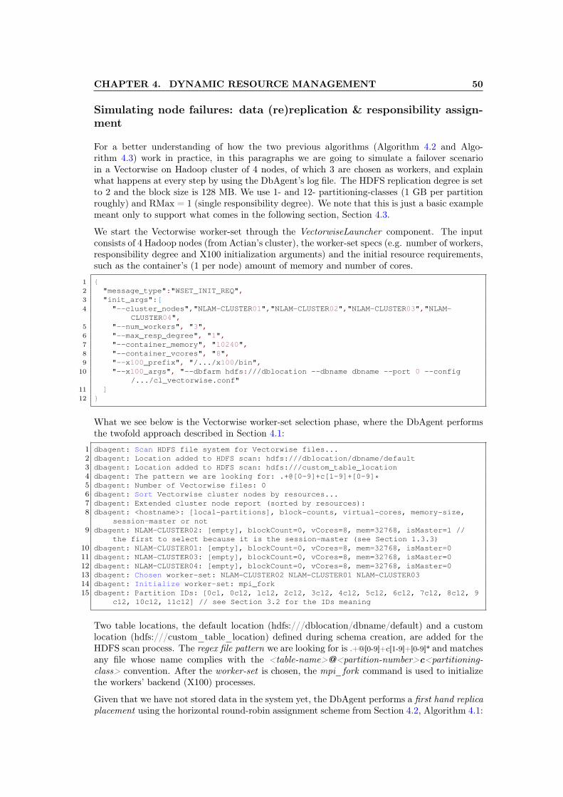
CHAPTER 4. DYNAMIC RESOURCE MANAGEMENT 50
Simulating node failures: data (re)replication & responsibility assign-ment
For a better understanding of how the two previous algorithms (Algorithm 4.2 and Algo-rithm 4.3) work in practice, in this paragraphs we are going to simulate a failover scenarioin a Vectorwise on Hadoop cluster of 4 nodes, of which 3 are chosen as workers, and explainwhat happens at every step by using the DbAgent’s log file. The HDFS replication degree is setto 2 and the block size is 128 MB. We use 1- and 12- partitioning-classes (1 GB per partitionroughly) and RMax = 1 (single responsibility degree). We note that this is just a basic examplemeant only to support what comes in the following section, Section 4.3.
We start the Vectorwise worker-set through the VectorwiseLauncher component. The inputconsists of 4 Hadoop nodes (from Actian’s cluster), the worker-set specs (e.g. number of workers,responsibility degree and X100 initialization arguments) and the initial resource requirements,such as the container’s (1 per node) amount of memory and number of cores.
1 {2 "message_type":"WSET_INIT_REQ",3 "init_args":[4 "--cluster_nodes","NLAM-CLUSTER01","NLAM-CLUSTER02","NLAM-CLUSTER03","NLAM-
CLUSTER04",5 "--num_workers", "3",6 "--max_resp_degree", "1",7 "--container_memory", "10240",8 "--container_vcores", "8",9 "--x100_prefix", "/.../x100/bin",
10 "--x100_args", "--dbfarm hdfs:///dblocation --dbname dbname --port 0 --config/.../cl_vectorwise.conf"
11 ]12 }
What we see below is the Vectorwise worker-set selection phase, where the DbAgent performsthe twofold approach described in Section 4.1:
1 dbagent: Scan HDFS file system for Vectorwise files...2 dbagent: Location added to HDFS scan: hdfs:///dblocation/dbname/default3 dbagent: Location added to HDFS scan: hdfs:///custom_table_location4 dbagent: The pattern we are looking for: .+@[0-9]+c[1-9]+[0-9]*5 dbagent: Number of Vectorwise files: 06 dbagent: Sort Vectorwise cluster nodes by resources...7 dbagent: Extended cluster node report (sorted by resources):8 dbagent: <hostname>: [local-partitions], block-counts, virtual-cores, memory-size,
session-master or not9 dbagent: NLAM-CLUSTER02: [empty], blockCount=0, vCores=8, mem=32768, isMaster=1 //
the first to select because it is the session-master (see Section 1.3.3)10 dbagent: NLAM-CLUSTER01: [empty], blockCount=0, vCores=8, mem=32768, isMaster=011 dbagent: NLAM-CLUSTER03: [empty], blockCount=0, vCores=8, mem=32768, isMaster=012 dbagent: NLAM-CLUSTER04: [empty], blockCount=0, vCores=8, mem=32768, isMaster=013 dbagent: Chosen worker-set: NLAM-CLUSTER02 NLAM-CLUSTER01 NLAM-CLUSTER0314 dbagent: Initialize worker-set: mpi_fork15 dbagent: Partition IDs: [0c1, 0c12, 1c12, 2c12, 3c12, 4c12, 5c12, 6c12, 7c12, 8c12, 9
c12, 10c12, 11c12] // see Section 3.2 for the IDs meaning
Two table locations, the default location (hdfs:///dblocation/dbname/default) and a customlocation (hdfs:///custom_table_location) defined during schema creation, are added for theHDFS scan process. The regex file pattern we are looking for is .+@[0-9]+c[1-9]+[0-9]* and matchesany file whose name complies with the <table-name>@<partition-number>c<partitioning-class> convention. After the worker-set is chosen, the mpi_fork command is used to initializethe workers’ backend (X100) processes.
Given that we have not stored data in the system yet, the DbAgent performs a first hand replicaplacement using the horizontal round-robin assignment scheme from Section 4.2, Algorithm 4.1:

CHAPTER 4. DYNAMIC RESOURCE MANAGEMENT 51
1 dbagent: First hand replica placement (round-robin), HDFS replication degree = 22 dbagent: For pClass = 1 (non-partitioned)3 dbagent: Node NLAM-CLUSTER02, max-partition-load is 14 dbagent: Node NLAM-CLUSTER01, max-partition-load is 15 dbagent: Node NLAM-CLUSTER03, max-partition-load is 06 dbagent: Assignment stats:7 dbagent: <hostname>: [responsibilities][local-partitions]8 dbagent: NLAM-CLUSTER02: [empty][0c1]9 dbagent: NLAM-CLUSTER01: [empty][0c1]
10 dbagent: NLAM-CLUSTER03: [empty][___]11 dbagent: For pClass = 12 (partitioned)12 dbagent: Node NLAM-CLUSTER02, max-partition-load is 813 dbagent: Node NLAM-CLUSTER01, max-partition-load is 814 dbagent: Node NLAM-CLUSTER03, max-partition-load is 815 dbagent: Assignment stats:16 dbagent: <hostname>: [responsibilities][local-partitions]17 dbagent: NLAM-CLUSTER02: [empty][0c1, 0c12, 3c12, 6c12, 9c12, 2c12, 5c12, 8c12, 11
c12]18 dbagent: NLAM-CLUSTER01: [empty][0c1, 1c12, 4c12, 7c12, 10c12, 0c12, 3c12, 6c12, 9
c12]19 dbagent: NLAM-CLUSTER03: [empty][___, 2c12, 5c12, 8c12, 11c12, 1c12, 4c12, 7c12, 10
c12]20 dbagent: (Re)Assigning responsibilities to worker nodes, RMax = 121 dbagent: For pClass = 12 (partitioned)22 dbagent: [0c12, 1c12, 2c12, 3c12, 4c12, 5c12, 6c12, 7c12, 8c12, 9c12, 10c12, 11c12]23 dbagent: Node NLAM-CLUSTER02, max-partition-load is 424 dbagent: Node NLAM-CLUSTER01, max-partition-load is 425 dbagent: Node NLAM-CLUSTER03, max-partition-load is 426 dbagent: Assignment done: flow = 12, cost = 1227 dbagent: Assignment stats:28 dbagent: <hostname>: [responsibilities][local-partitions]29 dbagent: NLAM-CLUSTER02: [0c12, 3c12, 5c12, 9c12][0c1, 0c12, 3c12, 6c12, 9c12, 2
c12, 5c12, 8c12, 11c12]30 dbagent: NLAM-CLUSTER01: [1c12, 4c12, 6c12, 7c12][0c1, 1c12, 4c12, 7c12, 10c12, 0
c12, 3c12, 6c12, 9c12]31 dbagent: NLAM-CLUSTER03: [2c12, 8c12, 10c12, 11c12][___, 2c12, 5c12, 8c12, 11c12, 1
c12, 4c12, 7c12, 10c12]32 dbagent: (Over)Writing the worker-set plocations metadata file33 dbagent: (Over)Writing the worker-set passignment metadata file
We now fast-forward to a situation where we have bulk-loaded data in the Vectorwise database,1 GB per partition (a non-partitioned table of 1 GB and a partitioned table of 12 GB). If nothingwent wrong (i.e. node failure) happens to the system and we restart the Vectorwise on Hadoopdatabase using the same request parameters, we notice that (1) HDFS finds the Vectorwisefiles’ locations and that (2) we can automatically match the table partitions to the worker nodeswith respect to data-locality and load-balancing factors. Since these files are still located onthe same workers (nothing is changed compared to the initial round-robin assignment), all12 partitions are distributed equally among our worker-set with cost 0. The same applies toassigning responsibilities: DbAgent assigns 4 responsibilities per worker node with 0 costs, ituses the last responsibility assignment (historical information) to adjust the cost model for thelocal "OS cached" partitions, Section 4.2. We can see all these steps in the following section ofthe log file:
1 dbagent: Scan HDFS file system for Vectorwise files...2 dbagent: Location added to HDFS scan: hdfs:///dblocation/dbname/default [1-file]3 dbagent: Location added to HDFS scan: hdfs:///custom_table_location [12-files]4 dbagent: The pattern we are looking for: .+@[0-9]+c[1-9]+[0-9]*5 dbagent: Number of Vectorwise files: 136 dbagent: Sort Vectorwise cluster nodes by resources...7 dbagent: Extended cluster node report (sorted by resources):8 dbagent: <hostname>: [local-partitions], block-counts, virtual-cores, memory-size,
session-master or not9 dbagent: NLAM-CLUSTER02: [0c1, 0c12, 3c12, 6c12, 9c12, 2c12, 5c12, 8c12, 11c12],
blockCount=72, vCores=8, mem=32768, isMaster=1

CHAPTER 4. DYNAMIC RESOURCE MANAGEMENT 52
10 dbagent: NLAM-CLUSTER01: [0c1, 1c12, 4c12, 7c12, 10c12, 0c12, 3c12, 6c12, 9c12],blockCount=72, vCores=8, mem=32768, isMaster=0
11 dbagent: NLAM-CLUSTER03: [___, 2c12, 5c12, 8c12, 11c12, 1c12, 4c12, 7c12, 10c12],blockCount=64, vCores=8, mem=32768, isMaster=0
12 dbagent: NLAM-CLUSTER04: [], blockCount=0, vCores=8, mem=32768, isMaster=013 dbagent: Chosen worker-set: NLAM-CLUSTER02 NLAM-CLUSTER01 NLAM-CLUSTER0314 dbagent: Initialize worker-set: mpi_fork15 dbagent: Partition IDs: [0c1, 0c12, 1c12, 2c12, 3c12, 4c12, 5c12, 6c12, 7c12, 8c12, 9
c12, 10c12, 11c12]16 dbagent: (Re)Matching table partitions to worker nodes, HDFS replication degree = 217 dbagent: No missing replicas18 .......19 dbagent: Assignment stats:20 dbagent: <hostname>: [responsibilities][local-partitions]21 dbagent: NLAM-CLUSTER02: [][0c1, 0c12, 3c12, 6c12, 9c12, 2c12, 5c12, 8c12, 11c12]22 dbagent: NLAM-CLUSTER01: [][0c1, 1c12, 4c12, 7c12, 10c12, 0c12, 3c12, 6c12, 9c12]23 dbagent: NLAM-CLUSTER03: [][___, 2c12, 5c12, 8c12, 11c12, 1c12, 4c12, 7c12, 10c12]24 dbagent: (Re)Assigning responsibilities to worker nodes, RMax = 125 dbagent: For pClass = 12 (partitioned)26 dbagent: [0c12, 1c12, 2c12, 3c12, 4c12, 5c12, 6c12, 7c12, 8c12, 9c12, 10c12, 11c12]27 dbagent: Passignment metadata file exists: adjusts costs for ex-responsibilities28 dbagent: Node NLAM-CLUSTER02, max-partition-load is 429 dbagent: Node NLAM-CLUSTER01, max-partition-load is 430 dbagent: Node NLAM-CLUSTER03, max-partition-load is 431 dbagent: Assignment done: flow = 12, cost = 032 dbagent: Assignment stats:33 dbagent: <hostname>: [responsibilities][local-partitions]34 dbagent: NLAM-CLUSTER02: [0c12, 3c12, 5c12, 9c12][0c1, 0c12, 3c12, 6c12, 9c12, 2
c12, 5c12, 8c12, 11c12] // ex-resp.35 dbagent: NLAM-CLUSTER01: [1c12, 4c12, 6c12, 7c12][0c1, 1c12, 4c12, 7c12, 10c12, 0
c12, 3c12, 6c12, 9c12] // ex-resp.36 dbagent: NLAM-CLUSTER03: [2c12, 8c12, 10c12, 11c12][___, 2c12, 5c12, 8c12, 11c12, 1
c12, 4c12, 7c12, 10c12] // ex-resp.37 dbagent: (Over)Writing the worker-set plocations metadata file38 dbagent: (Over)Writing the worker-set passignment metadata file
However, when a worker node fails (the third node), the DbAgent removes it from the Vectorwiseworker-set and selects a new Hadoop node as a replacement for the failed one. Missing replicasare identified and so, the new node is used for re-replication. In our case, the cost model formatching table partitions to worker nodes keeps the local partitions that were already storedamong the 1st and 2nd nodes intact and assigns (re-replicates) those that belonged to the 3rdnode to the 4th node instead (its partition capacity is 8). The cost that we get after performingthe min-cost flow is 8, equal to the number of partitions to be re-assigned and scheduled forre-replication to node 4. Our 4th (new empty) node did not have any local data beforehand.In the bipartite graph, all its in-edges from the table partitions were labeled with cost 1 ∼remote access. Furthermore, the new node was not part of the last Vectorwise worker-set,so it is assigned 4 responsibilities with cost 4 – basically the same responsibilities the 3rdnode previously had. But, since these responsibilities did not appear in the last responsibilityassignment, the costs were not adjusted to 0 ∼ local+. The following log section confirms whatwe have just explained:
1 dbagent: Scan HDFS file system for Vectorwise files...2 dbagent: Location added to HDFS scan: hdfs:///dblocation/dbname/default [1-file]3 dbagent: Location added to HDFS scan: hdfs:///custom_table_location [12-files]4 dbagent: The pattern we are looking for: .+@[0-9]+c[1-9]+[0-9]*5 dbagent: Number of Vectorwise files: 136 dbagent: Sort Vectorwise cluster nodes by resources...7 dbagent: Extended cluster node report (sorted by resources):8 dbagent: <hostname>: [local-partitions], block-counts, virtual-cores, memory-size,
session-master or not9 dbagent: NLAM-CLUSTER02: [0c1, 0c12, 3c12, 6c12, 9c12, 2c12, 5c12, 8c12, 11c12],
blockCount=72, vCores=8, mem=32768, isMaster=110 dbagent: NLAM-CLUSTER01: [0c1, 1c12, 4c12, 7c12, 10c12, 0c12, 3c12, 6c12, 9c12],
blockCount=72, vCores=8, mem=32768, isMaster=0
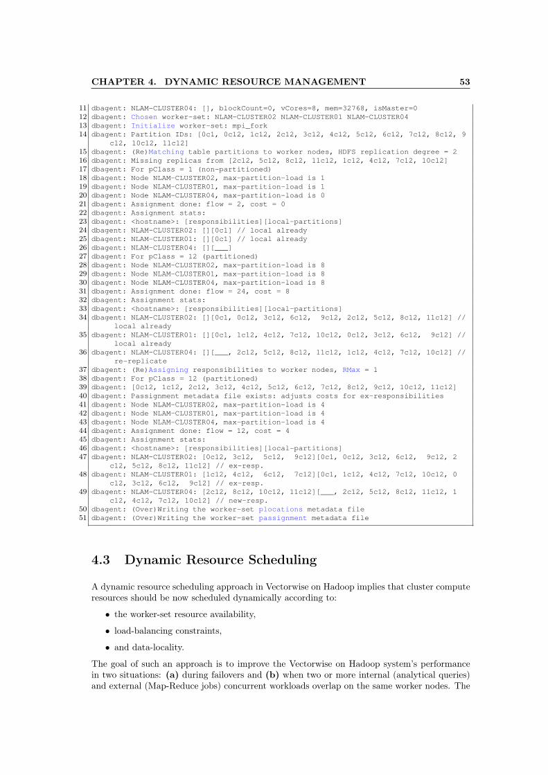
CHAPTER 4. DYNAMIC RESOURCE MANAGEMENT 53
11 dbagent: NLAM-CLUSTER04: [], blockCount=0, vCores=8, mem=32768, isMaster=012 dbagent: Chosen worker-set: NLAM-CLUSTER02 NLAM-CLUSTER01 NLAM-CLUSTER0413 dbagent: Initialize worker-set: mpi_fork14 dbagent: Partition IDs: [0c1, 0c12, 1c12, 2c12, 3c12, 4c12, 5c12, 6c12, 7c12, 8c12, 9
c12, 10c12, 11c12]15 dbagent: (Re)Matching table partitions to worker nodes, HDFS replication degree = 216 dbagent: Missing replicas from [2c12, 5c12, 8c12, 11c12, 1c12, 4c12, 7c12, 10c12]17 dbagent: For pClass = 1 (non-partitioned)18 dbagent: Node NLAM-CLUSTER02, max-partition-load is 119 dbagent: Node NLAM-CLUSTER01, max-partition-load is 120 dbagent: Node NLAM-CLUSTER04, max-partition-load is 021 dbagent: Assignment done: flow = 2, cost = 022 dbagent: Assignment stats:23 dbagent: <hostname>: [responsibilities][local-partitions]24 dbagent: NLAM-CLUSTER02: [][0c1] // local already25 dbagent: NLAM-CLUSTER01: [][0c1] // local already26 dbagent: NLAM-CLUSTER04: [][___]27 dbagent: For pClass = 12 (partitioned)28 dbagent: Node NLAM-CLUSTER02, max-partition-load is 829 dbagent: Node NLAM-CLUSTER01, max-partition-load is 830 dbagent: Node NLAM-CLUSTER04, max-partition-load is 831 dbagent: Assignment done: flow = 24, cost = 832 dbagent: Assignment stats:33 dbagent: <hostname>: [responsibilities][local-partitions]34 dbagent: NLAM-CLUSTER02: [][0c1, 0c12, 3c12, 6c12, 9c12, 2c12, 5c12, 8c12, 11c12] //
local already35 dbagent: NLAM-CLUSTER01: [][0c1, 1c12, 4c12, 7c12, 10c12, 0c12, 3c12, 6c12, 9c12] //
local already36 dbagent: NLAM-CLUSTER04: [][___, 2c12, 5c12, 8c12, 11c12, 1c12, 4c12, 7c12, 10c12] //
re-replicate37 dbagent: (Re)Assigning responsibilities to worker nodes, RMax = 138 dbagent: For pClass = 12 (partitioned)39 dbagent: [0c12, 1c12, 2c12, 3c12, 4c12, 5c12, 6c12, 7c12, 8c12, 9c12, 10c12, 11c12]40 dbagent: Passignment metadata file exists: adjusts costs for ex-responsibilities41 dbagent: Node NLAM-CLUSTER02, max-partition-load is 442 dbagent: Node NLAM-CLUSTER01, max-partition-load is 443 dbagent: Node NLAM-CLUSTER04, max-partition-load is 444 dbagent: Assignment done: flow = 12, cost = 445 dbagent: Assignment stats:46 dbagent: <hostname>: [responsibilities][local-partitions]47 dbagent: NLAM-CLUSTER02: [0c12, 3c12, 5c12, 9c12][0c1, 0c12, 3c12, 6c12, 9c12, 2
c12, 5c12, 8c12, 11c12] // ex-resp.48 dbagent: NLAM-CLUSTER01: [1c12, 4c12, 6c12, 7c12][0c1, 1c12, 4c12, 7c12, 10c12, 0
c12, 3c12, 6c12, 9c12] // ex-resp.49 dbagent: NLAM-CLUSTER04: [2c12, 8c12, 10c12, 11c12][___, 2c12, 5c12, 8c12, 11c12, 1
c12, 4c12, 7c12, 10c12] // new-resp.50 dbagent: (Over)Writing the worker-set plocations metadata file51 dbagent: (Over)Writing the worker-set passignment metadata file
4.3 Dynamic Resource Scheduling
A dynamic resource scheduling approach in Vectorwise on Hadoop implies that cluster computeresources should be now scheduled dynamically according to:
• the worker-set resource availability,
• load-balancing constraints,
• and data-locality.
The goal of such an approach is to improve the Vectorwise on Hadoop system’s performancein two situations: (a) during failovers and (b) when two or more internal (analytical queries)and external (Map-Reduce jobs) concurrent workloads overlap on the same worker nodes. The

CHAPTER 4. DYNAMIC RESOURCE MANAGEMENT 54
outcome of the resource scheduler is called a footprint and contains runtime information aboutthe worker nodes, the responsibilities (table partitions), and the number of threads per workerthat are involved in query execution. We refer to the query’s footprint in next paragraphs asthe resource footprint.
The problem to solve is not trivial at all. By all means, a good approach should (1) inform X100about the resource availability (e.g. number of available cores, free amount of memory), (2)achieve the maximum parallelism level (or mpl, i.e. the maximum number of threads to use forthat query’s execution) of a query by just using the workers’ available resources proportionallyto their partition locality, (3) determine, given the responsibility assignment, what are theworker nodes and partitions to be involved in the computation, and, at the same time, (4)improve data-locality. More details about (1), plus on how we use YARN to claim the resourcefootprint, are presented in Chapter 5.
On the other hand, to tackle (2), (3), and (4), we have enhanced the existent Vectorwiseresource scheduler with a min-cost flow algorithm. Though the algorithm uses a slightly moreadvanced cost model, Figure 4.5, the flow network (bipartite graph) is partitioned exactly asbefore. In addition, we extend our two previous ideas, matching partition tables and assigningresponsibilities to worker nodes, and use the last algorithm’s (Algorithm 4.3) result as inputto our new problem. As will see, the min-cost flow algorithm’s implementation, the successiveshortest path [49], is the common nominator of this chapter.
Successive Shortest Path. The successive shortest path algorithm searches for the maximumflow and optimizes the objective cost function simultaneously. It solves the so-called max-flowmin-cost problem by using the following idea. Suppose we have a flow network G and we haveto find an optimal flow across it. As we described in Section 2.3, the flow network is a directedgraph defined by a set V of vertexes (nodes) and set E of edges (arcs). For each edge weassociate a capacity uij , denotes the maximum amount of flow that can pass through the edge.Each edge also has an associated cost cij that stands as the cost per unit flow. We associatewith each vertex a number bi. This values represent the supply or the demand of the vertex. Ifbi > 0, node i is a supply node, else if bi < 0, node i is a demand node (its demand is equal to−bi). We call vertex i a transportation node if bi is zero. We further transform the network byadding two vertexes s and t (source and destination) and some edges as follows: for each nodei in V (the set of vertexes), we add a source arc (s, i) with capacity usi = bi and csi = 0. Foreach node i in V with bi < 0, we add a sink edge (i, t) with capacity uit = −bi and cit = 0.Then, instead of searching for the maximum flow as usual, we send flow from s to t along theshortest path (with respect to arc costs). Next we update the residual network, find anothershortest path and augment the flow again, and so on. The algorithm terminates when theresidual network contains no path from s to t (the flow is maximal). A high-level pseudocodeto summarize the before-mentioned steps is as follows:
1 // Successive Shortest Path Algorithm2 Transform network G by adding source (s) and destination (t)3 Initial flow x is zero4 while ( G(x) contains a path from s to t ) do5 Find any shortest path P from s to t6 Augment current flow x along P7 Update G(x)
Since the flow is maximal, it corresponds to a feasible solution of the original min-cost flowproblem. Moreover, this solution will be optimal [49]. The successive shortest path algorithmcan be used when G contains no negative cost cycles. Otherwise, we cannot say exactly whatthe shortest path means.
The successive shortest path pseudocode from above was molded to our purposes (for Fig-ure 4.2, 4.4, 4.5 flow networks). The transformation from line 2 applies to a bipartite graphG instead. In this case V = {P,W} is the set of vertexes, where P = {partitions, ...} is the
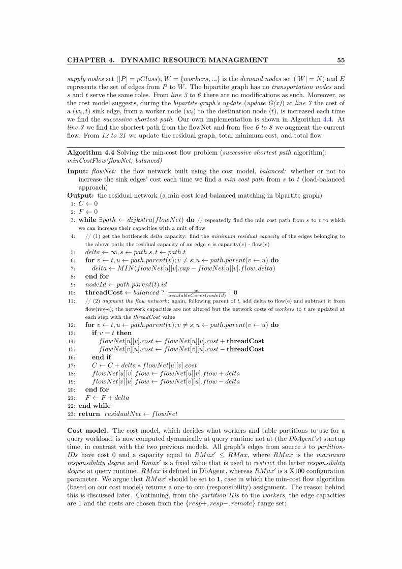
CHAPTER 4. DYNAMIC RESOURCE MANAGEMENT 55
supply nodes set (|P | = pClass), W = {workers, ...} is the demand nodes set (|W | = N) and Erepresents the set of edges from P to W . The bipartite graph has no transportation nodes ands and t serve the same roles. From line 3 to 6 there are no modifications as such. Moreover, asthe cost model suggests, during the bipartite graph’s update (update G(x)) at line 7 the cost ofa (wi, t) sink edge, from a worker node (wi) to the destination node (t), is increased each timewe find the successive shortest path. Our own implementation is shown in Algorithm 4.4. Atline 3 we find the shortest path from the flowNet and from line 6 to 8 we augment the currentflow. From 12 to 21 we update the residual graph, total minimum cost, and total flow.
Algorithm 4.4 Solving the min-cost flow problem (successive shortest path algorithm):minCostFlow(flowNet, balanced)
Input: flowNet: the flow network built using the cost model, balanced: whether or not toincrease the sink edges’ cost each time we find a min cost path from s to t (load-balancedapproach)
Output: the residual network (a min-cost load-balanced matching in bipartite graph)1: C ← 02: F ← 03: while ∃path ← dijkstra(flowNet) do // repeatedly find the min cost path from s to t to which
we can increase their capacities with a unit of flow4: // (1) get the bottleneck delta capacity: find the minimum residual capacity of the edges belonging to
the above path; the residual capacity of an edge e is capacity(e) - flow(e)5: delta←∞, s← path.s, t← path.t6: for v ← t, u← path.parent(v); v 6= s;u← path.parent(v ← u) do7: delta←MIN(flowNet[u][v].cap− flowNet[u][v].f low, delta)8: end for9: nodeId← path.parent(t).id
10: threadCost← balanced ? wi
availableCores(nodeId) : 011: // (2) augment the flow network : again, following parent of t, add delta to flow(e) and subtract it from
flow(rev-e); the network capacities are not altered but the network costs of workers to t are updated ateach step with the threadCost value
12: for v ← t, u← path.parent(v); v 6= s;u← path.parent(v ← u) do13: if v = t then14: flowNet[u][v].cost← flowNet[u][v].cost+ threadCost15: flowNet[v][u].cost← flowNet[v][u].cost− threadCost16: end if17: C ← C + delta ∗ flowNet[u][v].cost18: flowNet[u][v].f low ← flowNet[u][v].f low + delta19: flowNet[v][u].f low ← flowNet[v][u].f low − delta20: end for21: F ← F + delta22: end while23: return residualNet← flowNet
Cost model. The cost model, which decides what workers and table partitions to use for aquery workload, is now computed dynamically at query runtime not at (the DbAgent’s) startuptime, in contrast with the two previous models. All graph’s edges from source s to partition-IDs have cost 0 and a capacity equal to RMax′ ≤ RMax, where RMax is the maximumresponsibility degree and Rmax′ is a fixed value that is used to restrict the latter responsibilitydegree at query runtime. RMax is defined in DbAgent, whereas RMax′ is a X100 configurationparameter. We argue that RMax′ should be set to 1, case in which the min-cost flow algorithm(based on our cost model) returns a one-to-one (responsibility) assignment. The reason behindthis is discussed later. Continuing, from the partition-IDs to the workers, the edge capacitiesare 1 and the costs are chosen from the {resp+, resp−, remote} range set:

CHAPTER 4. DYNAMIC RESOURCE MANAGEMENT 56
• resp+ = LLi, the worker’s up-to-date load factor
– this capacity is attributed to (partition) responsibilities which are local to theworker nodes
– the new LLi load factor is aware of both, the internal and external workloads (i.e.the number of used cores)
– it is based on Section 1.3.2’s load factor early formula, except that Ti (the threadload on worker i) is now redefined as internalThreadsi+externalThreadsi
Ci, where Ci is the
total number of cores on worker i (i.e. the max cores capability)
– resp+ cost should be able to make a difference between the various load factors,such that we favor the least loaded nodes for running the current Vectorwise query
• resp− = LLi + wi, the worker’s load factor plus a penalty
– this capacity is attributed to (partition) responsibilities which are not yet local tothe worker nodes (i.e. are still during re-replication), we refer to it with partial (partition)responsibilities
– adding the wi thread weight (Section 1.3.2) to the upper formula creates a costgap between the local and partial (partition) responsibilities; we choose wi just to beconsistent with the surrounding developed code, as well this penalty can be set to anydifferent constant value
– the cost gap is reduced when almost all local (partition) responsibilities have beenassigned while running the min-cost flow algorithm, in which case some of the partial(partition) responsibilities will start being assigned to the least loaded nodes
– to determine the partial (partition) responsibilities from the passignment metadata,an up-to-date snapshot of the Vectorwise block locations is needed; more about this innext Chapter 5
• remote = LLi + wi ∗ penalty, the worker’s load factor plus a magnified penalty
– this capacity is attributed to all the remaining partitions of which the worker nodesare not responsible for
– a 1.25 value for the penalty is determined experimentally to take in account (asits best) remote (partition) responsibilities; we multiply wi by this penalty in order toreduce the likelihood of remote (partition) responsibilities being assigned (over local oreven partial ones) to worker nodes while running the min-cost flow algorithm
Finally, each edge from a worker to the destination vertex t has the capacity equal to theworker’s partition capacity (PCap, see Section 4.1) and its cost is expressed as a TCost :N → N function, TCost(fx) = fx ∗ threadCost – increases each time we select the shortestpath during the while-loop (step x ) of Algorithm 4.4. Note that, we consider RMax ≤ R tobenefit from data-locality and to make sure that all of a worker’s (partition) responsibilitiesare either local or, at most, partial responsibilities. Moreover, because we do not have anymemory requirements for queries as such, the worker’s partition capacity is simply figured asPCapi = availableCoresi ∗ core_overalloc, i = 1, . . . , N , where availableCoresi informationis always up-to-date and core_overalloc is a system configuration parameter.
We shortly remind that in Vectorwsie distributed MPP version the resource scheduling algorithmprovides us a list of pairs (nx, ty) denoting how many threads/cores (ty) are allocated for itsexecution on node (nx). The search starts with a feasible (initial) solution and tries/verifiesall its multiple (e.g. [(1, 3), (2, 5)] : [(1, 6), (2, 10)] : [(1, 9), (2, 15)] : etc . . .). It stops at thefirst combination which uses more threads (on any machine) than allocated by the resourcescheduler. Moreover, from Section 1.3.3, we know that the algorithm uses two multiple-nodes

CHAPTER 4. DYNAMIC RESOURCE MANAGEMENT 57
Figure 4.5: The flow network (bipartite graph) model used to calculate a part of the resourcefootprint (what nodes and table partitions we use for a query, given the worker’s availableresource and data-locality). Note: fx is the unit with which we increase the flow along thepath at step x of the algorithm.
distribution policies for queries: (1) equal share for non-partitioned tables, which similar withthe multiple-nodes distribution used in the Shared Disk approach it selects the least loadednodes and takes their amount of CPU resources until it satisfies the mpl and (2) equal share forpartitioned tables that assumes the default round-robin partitioning and equally assigns threadsto the operators until the mpl is achieved.
The new dynamic approach tries to combine these policies within a min-cost flow algorithm. So,ideally, we must find the smallest subset of workers that fulfills the maximum parallelism levelof a query with respect to the worker-set current data-locality and load-balancing constraintsimposed by the outside world (i.e. other workloads sharing the same Hadoop infrastructure).In this form, the problem is similar to the weighted set covering problem [51, 52]. Given a setof elements U = {1, 2, ...,m} (called the universe) and a S of n sets whose union equals theuniverse, the set covering problem [51] is to identify the smallest subset of S whose union equalsthe universe. For example, consider the universe U = {1, 2, 3, 4, 5, 6} and the set of sets S ={{1, 2, 3}, {2, 4}, {3, 4}, {4, 5}, {5, 6}}. Clearly the union of S is U . However, we can cover all ofthe elements with one of the following, smaller number of sets solutions: {{1, 2, 3}, {3, 4}, {5, 6}},{{1, 2, 3}, {2, 4}, {5, 6}}, or {{1, 2, 3}, {4, 5}, {5, 6}}. More formally, given the universe U anda family S of subsets of U , a cover is a subfamily C ⊆ S of sets whose union is U . In the setcovering decision problem, the input is a pair (U, S) and an integer k; the question is whetherthere is a set covering of size k or less. In the set covering optimization problem, the input is apair (U, S), and the task is to find a set covering that uses the fewest sets. The decision versionof the set covering problem is NP-complete [53], and the optimization version is NP-hard. Ifadditionally, you want to minimize the cost of the set cover (costs > 1), the problem becomes aweighted set covering problem. The latter is by definition an optimization variant as well, whichmakes it NP-hard to solve.
Moreover, the set covering problem can be reduced to bipartite graphs: an instance of the setcovering can be viewed as an arbitrary bipartite graph, with sets represented by vertices on

CHAPTER 4. DYNAMIC RESOURCE MANAGEMENT 58
the left, the universe represented by vertices on the right, and edges representing the inclusionof elements in sets. The task is then to find a minimum cardinality subset of left-verticeswhich covers all of the right-vertices. In the hitting set problem citeset-covering-hitting-set, theobjective is to cover the left-vertices using a minimum subset of the right vertices. Convertingfrom one problem to the other is therefore achieved by interchanging the two sets of vertices. Ifthe graph’s edges has costs then it becomes the weighted hitting set problem. Though it soundssimilar to a min-cost flow problem, just applying the successive shortest path algorithm will notresult in finding the perfect (optimal cost minimal subset) solution. Only the representation ofthe problem changes, but its complexity (NP-hard) remains the same. Any general polynomial-time algorithm, such as the successive shortest path, that always outputs the optimal solution toour optimization problem would imply that P=NP (which is quite improbable). Instead, whatwe actually need is an approximation algorithm for the problem, or, more likely, an heuristicalgorithm.
One thing to do, is to take advantage of the HDFS local replicas. Increasing the RMax (themaximum responsibility degree, see Section 4.2) value per partition, up to the HDFS replica-tion degree, adds a certain elasticity in computing an optimal resource footprint for a queryworkload. With it, we can vary the available resources from 1 thread per node to the maximumthreads possible per partition and, at the same time, choose what worker nodes to involve in thecomputation. In this way, we can reduce the (resource) contention with other jobs sharing thesame cluster. For instance, the algorithm can choose just a few workers from the worker-set torun a Vectorwise query. This may happen in case some workers are overloaded or facing otherproblems, e.g. no local-data due to a failure. With RMax’ = 1 we can restrict the maximumresponsibility degree at runtime and instead compute multiple one-to-one assignment (optimalcost) solutions (e.g. different workers, different partitions, etc.), of which just some will beof minimum size as well. It all depends on the data-locality, load-factors, etc., for the flow-algorithm to determine a starting feasible solution, a one-to-one assignment that allows us toscale with the number of threads up to the maximum level of parallelism. The latter, as willsee in Chapter 5, leads to computing the resource footprint. Of course, for this to happen, theHDFS replication degree should be ≥ 2 and so the RMax as well.
Figure 4.6: Selecting the (partition responsibilities and worker nodes involved in query execu-tion. Only the first two workers from left are chosen (bold-italic black) for table scans; firstone reads from two partitions (red and green), whereas the second reads just from one (blue).The third worker is considered overloaded and so, it is excluded from the I/O. Red/blue/greencolors are used to express multiple (partition) responsibilities.
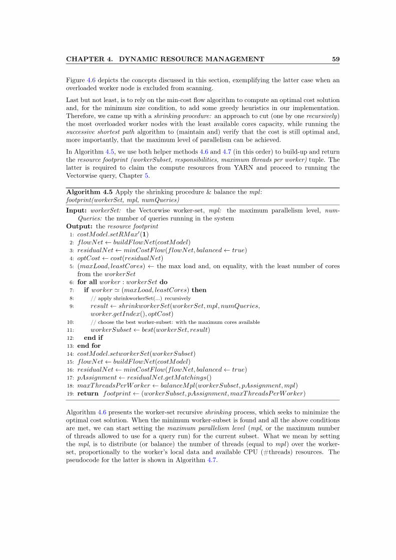
CHAPTER 4. DYNAMIC RESOURCE MANAGEMENT 59
Figure 4.6 depicts the concepts discussed in this section, exemplifying the latter case when anoverloaded worker node is excluded from scanning.
Last but not least, is to rely on the min-cost flow algorithm to compute an optimal cost solutionand, for the minimum size condition, to add some greedy heuristics in our implementation.Therefore, we came up with a shrinking procedure: an approach to cut (one by one recursively)the most overloaded worker nodes with the least available cores capacity, while running thesuccessive shortest path algorithm to (maintain and) verify that the cost is still optimal and,more importantly, that the maximum level of parallelism can be achieved.
In Algorithm 4.5, we use both helper methods 4.6 and 4.7 (in this order) to build-up and returnthe resource footprint (workerSubset, responsibilities, maximum threads per worker) tuple. Thelatter is required to claim the compute resources from YARN and proceed to running theVectorwise query, Chapter 5.
Algorithm 4.5 Apply the shrinking procedure & balance the mpl :footprint(workerSet, mpl, numQueries)
Input: workerSet: the Vectorwise worker-set, mpl: the maximum parallelism level, num-Queries: the number of queries running in the system
Output: the resource footprint1: costModel.setRMax′(1)2: flowNet← buildF lowNet(costModel)3: residualNet← minCostF low(flowNet, balanced← true)4: optCost← cost(residualNet)5: (maxLoad, leastCores) ← the max load and, on equality, with the least number of cores
from the workerSet6: for all worker : workerSet do7: if worker ' (maxLoad, leastCores) then8: // apply shrinkworkerSet(...) recursively9: result← shrinkworkerSet(workerSet,mpl, numQueries,
worker.getIndex(), optCost)10: // choose the best worker-subset: with the maximum cores available11: workerSubset← best(workerSet, result)12: end if13: end for14: costModel.setworkerSet(workerSubset)15: flowNet← buildF lowNet(costModel)16: residualNet← minCostF low(flowNet, balanced← true)17: pAssignment← residualNet.getMatchings()18: maxThreadsPerWorker ← balanceMpl(workerSubset, pAssignment,mpl)19: return footprint← (workerSubset, pAssignment,maxThreadsPerWorker)
Algorithm 4.6 presents the worker-set recursive shrinking process, which seeks to minimize theoptimal cost solution. When the minimum worker-subset is found and all the above conditionsare met, we can start setting the maximum parallelism level (mpl, or the maximum numberof threads allowed to use for a query run) for the current subset. What we mean by settingthe mpl, is to distribute (or balance) the number of threads (equal to mpl) over the worker-set, proportionally to the worker’s local data and available CPU (#threads) resources. Thepseudocode for the latter is shown in Algorithm 4.7.
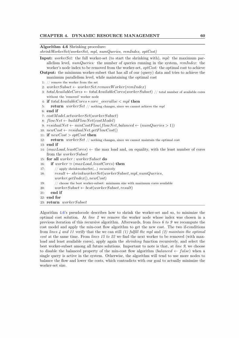
CHAPTER 4. DYNAMIC RESOURCE MANAGEMENT 60
Algorithm 4.6 Shrinking procedure:shrinkWorkerSet(workerSet, mpl, numQueries, remIndex, optCost)
Input: workerSet: the full worker-set (to start the shrinking with), mpl: the maximum par-allelism level, numQueries: the number of queries running in the system, remIndex: theworker’s node index to be removed from the worker-set, optCost: the optimal cost to achieve
Output: the minimum worker-subset that has all of our (query) data and tries to achieve themaximum parallelism level, while maintaining the optimal cost
1: // remove the worker from the set2: workerSubset← workerSet.removeWorker(remIndex)3: totalAvailableCores ← totalAvailableCores(workerSubset) // total number of available cores
without the ’removed’ worker node4: if totalAvailableCores ∗ core_overalloc < mpl then5: return workerSet // nothing changes, since we cannot achieve the mpl6: end if7: costModel.setworkerSet(workerSubset)8: flowNet← buildF lowNet(costModel)9: residualNet← minCostF low(flowNet, balanced← (numQueries > 1))
10: newCost← residualNet.getF lowCost()11: if newCost > optCost then12: return workerSet // nothing changes, since we cannot maintain the optimal cost13: end if14: (maxLoad, leastCores) ← the max load and, on equality, with the least number of cores
from the workerSubset15: for all worker : workerSubset do16: if worker ' (maxLoad, leastCores) then17: // apply shrinkworkerSet(...) recursively18: result← shrinkworkerSet(workerSubset,mpl, numQueries,
worker.getIndex(), newCost)19: // choose the best worker-subset: minimum size with maximum cores available20: workerSubset← best(workerSubset, result)21: end if22: end for23: return workerSubset
Algorithm 4.6’s pseudocode describes how to shrink the worker-set and so, to minimize theoptimal cost solution. At line 2 we remove the worker node whose index was chosen in aprevious iteration of this recursive algorithm. Afterwards, from lines 6 to 9 we recompute thecost model and apply the min-cost flow algorithm to get the new cost. The two if-conditionsfrom lines 4 and 11 verify that the we can still (1) fulfill the mpl and (2) maintain the optimalcost at the same time. From lines 15 to 22 we find the next worker to be removed (with max-load and least available cores), apply again the shrinking function recursively, and select thebest worker-subset among all future solutions. Important to note is that, at line 9, we chooseto disable the balanced property of the min-cost flow algorithm (balanced ← false) when asingle query is active in the system. Otherwise, the algorithm will tend to use more nodes tobalance the flow and lower the costs, which contradicts with our goal to actually minimize theworker-set size.

CHAPTER 4. DYNAMIC RESOURCE MANAGEMENT 61
Algorithm 4.7 Balance the mpl (#threads) on top of the current workers-(sub)set (∼ propor-tionally to the worker’s local data and available resources):balanceMpl(workerSet, pAssignment, mpl)
Input: workerSet: the workers-(sub)set, pAssignment: the responsibility assignment with re-spect to the new workers-(sub)set mpl: the maximum parallelism level
Output: array of maximum number of threads per worker node1: // distribute the mpl bounded number of threads over the worker-set, proportionally to the worker’s local
data (i.e. remaining partitions) and available CPU (#cores) resources2: remaining ← pAssignment.getPartitionsNum()3: for all worker : workerSet ∧mpl > 0 do4: current← pAssignment.getPartitionsFor(worker).size5: if current = 0 then6: cntZero← cntZero+ 17: continue8: end if9: ratio← mpl
remaining
10: threads← round(ratio ∗ current)11: threads←MIN(threads, worker.getAvailableCores() ∗ core_overalloc)12: worker.setThreads(threads)13: remaining ← remaining − current14: mpl← mpl − threads15: end for16: if cntZero = 0 ∨mpl = 0 then17: return maxThreadsPerWorker ← threadsPerWorker(workerSet)18: end if19: // equally redistribute the remaining threads (mpl) to what is left from the workers-(sub)set, to those
worker nodes that were not assigned with any partitions; if there are no such workers left, then the mpl isreduced to the cluster’s available CPU (#cores) capacity (with over-allocation)
20: equalShare← mpl/cntZero21: plusOne← mpl%cntZero22: i← 023: for all worker : workerSet ∧mpl > 0 do24: current← pAssignment.getPartitionsFor(worker).size25: if current > 0 then26: continue27: end if28: threads = i < plusOne ? (equalShare+ 1) : equalShare29: worker.setThreads(threads)30: mpl← mpl − threads31: i← i+ 132: end for33: return maxThreadsPerWorker ← threadsPerWorker(workerSet)
The above algorithm, Algorithm 4.7, tries to balance the mpl on top of the current workers-(sub)set and thus, to compute the maximum threads per worker for the query workload. Fromlines 2 to 15 we try to distribute threads (bounded by mpl) to the worker nodes, proportionallyto their local data (i.e. remaining partitions) and available CPU (#cores) resources (includingan over-allocation). If we cannot succeed to elapse all threads and achieve the mpl with oneshot, starting line 20 to 32 we equally redistribute the remaining mpl to those workers that wereleft unassigned (with responsibilities) after running the (balanced) min-cost flow algorithm.
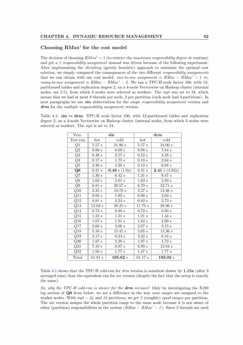
CHAPTER 4. DYNAMIC RESOURCE MANAGEMENT 62
Choosing RMax’ for the cost model
The decision of choosing RMax′ = 1 (to restrict the maximum responsibility degree at runtime)and get a 1 responsibility assignment instead was driven because of the following experiment.After implementing the shrinking (greedy heuristic) approach to minimize the optimal costsolution, we simply compared the consequences of the two different responsibility assignmentsthat we can obtain with our cost model: one-to-one assignment ≡ RMax = RMax’ = 1 vs.many-to-one assignment ≡ RMax = RMax’ = 2. We ran a TPC-H scale factor 100, with 12-partitioned tables and replication degree 2, on a 4-node Vectorwise on Hadoop cluster (internalnodes, see 2.5), from which 3 nodes were selected as workers. The mpl was set to 24, whichmeans that we had at most 8 threads per node, 2 per partition (each node had 4 partitions). Innext paragraphs we use sin abbreviation for the single responsibility assignment version anddrm for the multiple responsibility assignment version.
Table 4.1: sin vs drm: TPC-H scale factor 100, with 12-partitioned tables and replicationdegree 2, on a 4-node Vectorwise on Hadoop cluster (internal nodes, from which 3 nodes wereselected as workers. The mpl is set to 24.
Vers. sin drmTest-run hot cold hot cold
Q1 5.57 s 31.96 s 5.57 s 34.00 sQ2 0.99 s 6.69 s 0.98 s 7.84 sQ3 0.48 s 2.57 s 0.52 s 4.28 sQ4 0.17 s 1.75 s 0.18 s 2.64 sQ5 2.30 s 4.30 s 2.12 s 6.04 sQ6 0.31 s 0.49 s (1.0x) 0.31 s 2.41 s (4.92x)Q7 1.30 s 6.42 s 1.31 s 9.47 sQ8 1.63 s 5.01 s 1.63 s 5.93 sQ9 6.81 s 20.57 s 6.79 s 22.71 sQ10 3.35 s 10.79 s 3.37 s 13.46 sQ11 0.92 s 1.92 s 0.90 s 2.03 sQ12 0.81 s 3.24 s 0.82 s 3.73 sQ13 12.02 s 28.25 s 11.75 s 28.96 sQ14 0.73 s 0.80 s 0.72 s 0.80 sQ15 1.23 s 1.31 s 1.21 s 1.44 sQ16 1.67 s 1.91 s 1.62 s 2.00 sQ17 2.66 s 3.06 s 2.67 s 3.15 sQ18 5.16 s 15.41 s 5.05 s 15.36 sQ19 3.17 s 6.24 s 3.22 s 6.44 sQ20 1.87 s 2.29 s 1.97 s 4.72 sQ21 7.10 s 8.87 s 6.99 s 12.84 sQ22 1.56 s 1.77 s 1.47 s 1.77 sTotal 61.81 s 165.62 s 61.17 s 192.02 s
Table 4.1 shows that the TPC-H cold-run for drm version is somehow slower by 1.15x (after 3averaged runs) than the equivalent run for sin version (despite the fact that the setup is exactlythe same).
So, why the TPC-H cold-run is slower for the drm version? Only by investigating the X100log section of Q6 from below, we see a difference in the way scan ranges are assigned to theworker nodes. With mpl = 24 and 12 partitions, we get 2 (roughly) equal ranges per partition.The sin version assigns the whole partition range to the same node because it is not aware ofother (partition) responsibilities in the system (RMax = RMax’ = 1 ). Since 2 threads are used
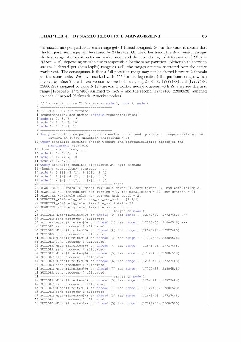
CHAPTER 4. DYNAMIC RESOURCE MANAGEMENT 63
(at maximum) per partition, each range gets 1 thread assigned. So, in this case, it means thatthe full partition range will be shared by 2 threads. On the other hand, the drm version assignsthe first range of a partition to one worker node and the second range of it to another (RMax =RMax’ = 2 ), depending on who else is responsible for the same partition. Although this versionassigns 1 thread per (equal-split) range as well, the ranges are now scattered over the entireworker-set. The consequence is that a full partition range may not be shared between 2 threadson the same node. We have marked with *** (in the log section) the partition ranges whichinvolve lineitem@0 : with sin version we see both ranges [12648448, 17727488) and [17727488,22806528) assigned to node 0 (2 threads, 1 worker node), whereas with drm we see the firstrange [12648448, 17727488) assigned to node 0 and the second [17727488, 22806528) assignedto node 1 instead (2 threads, 2 worker nodes).
1 // Log section from X100 workers: node 0, node 1, node 22 =====================================3 (1) TPC-H Q6, sin version4 Responsibility assignment (single responsibilities):5 node 0: 0, 3, 6, 96 node 1: 1, 4, 7, 107 node 2: 2, 5, 8, 118 =====================================9 Query scheduler: computing the min worker-subset and (partition) responsibilities to
involve in query execution (Algorithm 4.5)10 Query scheduler results: chosen workers and responsibilities (based on the
passignment metadata)11 <host>: <partition>, ...12 node 0: 0, 3, 6, 913 node 1: 1, 4, 7, 1014 node 2: 2, 5, 8, 1115 Query scheduler results: distribute 24 (mpl) threads16 <host>: <partition> [#threads], ...17 node 0: 0 [2], 3 [2], 6 [2], 9 [2]18 node 1: 1 [2], 4 [2], 7 [2], 10 [2]19 node 2: 2 [2], 5 [2], 8 [2], 11 [2]20 ===================================== Stats21 REWRITER_XCHG:parallel_mode: available_cores 24, core_target 30, max_parallelism 2422 REWRITER_XCHG:ccheduler: num_queries = 1, max_parallelism = 24, num_granted = 2423 REWRITER_XCHG:xchg_rule: max_tds_per_node total = 2424 REWRITER_XCHG:xchg_rule: max_tds_per_node = [8,8,8]25 REWRITER_XCHG:xchg_rule: feasible_sol total = 2426 REWRITER_XCHG:xchg_rule: feasible_sol = [8,8,8]27 ===================================== Ranges on node 028 BUILDER:MScan(lineitem@0) on thread [0] has range : [12648448, 17727488) ***29 BUILDER:send producer 0 allocated.30 BUILDER:MScan(lineitem@0) on thread [1] has range : [17727488, 22806528) ***31 BUILDER:send producer 1 allocated.32 BUILDER:MScan(lineitem@3) on thread [2] has range : [12648448, 17727488)33 BUILDER:send producer 2 allocated.34 BUILDER:MScan(lineitem@3) on thread [3] has range : [17727488, 22806528)35 BUILDER:send producer 3 allocated.36 BUILDER:MScan(lineitem@6) on thread [4] has range : [12648448, 17727488)37 BUILDER:send producer 4 allocated.38 BUILDER:MScan(lineitem@6) on thread [5] has range : [17727488, 22806528)39 BUILDER:send producer 5 allocated.40 BUILDER:MScan(lineitem@9) on thread [6] has range : [12648448, 17727488)41 BUILDER:send producer 6 allocated.42 BUILDER:MScan(lineitem@9) on thread [7] has range : [17727488, 22806528)43 BUILDER:send producer 7 allocated.44 ===================================== ranges on node 145 BUILDER:MScan(lineitem@1) on thread [0] has range : [12648448, 17727488)46 BUILDER:send producer 0 allocated.47 BUILDER:MScan(lineitem@1) on thread [1] has range : [17727488, 22806528)48 BUILDER:send producer 1 allocated.49 BUILDER:MScan(lineitem@4) on thread [2] has range : [12648448, 17727488)50 BUILDER:send producer 2 allocated.51 BUILDER:MScan(lineitem@4) on thread [3] has range : [17727488, 22806528)

CHAPTER 4. DYNAMIC RESOURCE MANAGEMENT 64
52 BUILDER:send producer 3 allocated.53 BUILDER:MScan(lineitem@7) on thread [4] has range : [12648448, 17727488)54 BUILDER:send producer 4 allocated.55 BUILDER:MScan(lineitem@7) on thread [5] has range : [17727488, 22806528)56 BUILDER:send producer 5 allocated.57 BUILDER:MScan(lineitem@10) on thread [6] has range : [12648448, 17727488)58 BUILDER:send producer 6 allocated.59 BUILDER:MScan(lineitem@10) on thread [7] has range : [17727488, 22806528)60 BUILDER:send producer 7 allocated.61 ===================================== ranges on node 262 BUILDER:MScan(lineitem@2) on thread [0] has range : [12648448, 17727488)63 vBUILDER:send producer 0 allocated.64 BUILDER:MScan(lineitem@2) on thread [1] has range : [17727488, 22806528)65 BUILDER:send producer 1 allocated.66 BUILDER:MScan(lineitem@5) on thread [2] has range : [12648448, 17727488)67 BUILDER:send producer 2 allocated.68 BUILDER:MScan(lineitem@5) on thread [3] has range : [17727488, 22806528)69 BUILDER:send producer 3 allocated.70 BUILDER:MScan(lineitem@8) on thread [4] has range : [12648448, 17727488)71 BUILDER:send producer 4 allocated.72 BUILDER:MScan(lineitem@8) on thread [5] has range : [17727488, 22806528)73 BUILDER:send producer 5 allocated.74 BUILDER:MScan(lineitem@11) on thread [6] has range : [12648448, 17727488)75 BUILDER:send producer 6 allocated.76 BUILDER:MScan(lineitem@11) on thread [7] has range : [17727488, 22806528)77 BUILDER:send producer 7 allocated.78 =====================================79 // (2) TPC-H Q6, drm version80 Responsibility assignment (multiple responsibilities):81 node 0: 0, 3, 6, 9, 2, 5, 8, 1182 node 1: 1, 4, 7, 10, 0, 3, 6, 983 node 2: 2, 5, 8, 11, 1, 4, 7, 1084 =====================================85 Query scheduler: computing the min worker-subset and (partition) responsibilities to
involve in query execution (Algorithm 4.5)86 Query scheduler results: chosen workers and responsibilities (based on the
passignment metadata)87 <host>: <partition>, ...88 node 0: 0, 3, 6, 9, 2, 5, 8, 1189 node 1: 1, 4, 7, 10, 0, 3, 6, 990 node 2: 2, 5, 8, 11, 1, 4, 7, 1091 Query scheduler results: distribute 24 (mpl) threads92 <host>: <partition> [#threads], ...93 node 0: 0 [1], 3 [1], 6 [1], 9 [1], 2 [1], 5 [1], 8 [1], 11 [1]94 node 1: 1 [1], 4 [1], 7 [1], 10 [1], 0 [1], 3 [1], 6 [1], 9 [1]95 node 2: 2 [1], 5 [1], 8 [1], 11 [1], 1 [1], 4 [1], 7 [1], 10 [1]96 ===================================== stats97 REWRITER_XCHG:parallel_mode: available_cores 24, core_target 30, max_parallelism 2498 REWRITER_XCHG:scheduler: num_queries = 1, max_parallelism = 24, num_granted = 2499 REWRITER_XCHG:xchg_rule: max_tds_per_node total = 24
100 REWRITER_XCHG:xchg_rule: max_tds_per_node = [8,8,8]101 REWRITER_XCHG:xchg_rule: feasible_sol total = 24102 REWRITER_XCHG:xchg_rule: feasible_sol = [8,8,8]103 ===================================== ranges on node 0104 BUILDER:MScan(lineitem@0) on thread [0] has range : [12648448, 17727488) ***105 BUILDER:send producer 0 allocated.106 BUILDER:MScan(lineitem@2) on thread [1] has range : [12648448, 17727488)107 BUILDER:send producer 1 allocated.108 BUILDER:MScan(lineitem@3) on thread [2] has range : [12648448, 17727488)109 BUILDER:send producer 2 allocated.110 BUILDER:MScan(lineitem@5) on thread [3] has range : [12648448, 17727488)111 BUILDER:send producer 3 allocated.112 BUILDER:MScan(lineitem@6) on thread [4] has range : [12648448, 17727488)113 BUILDER:send producer 4 allocated.114 BUILDER:MScan(lineitem@8) on thread [5] has range : [12648448, 17727488)115 BUILDER:send producer 5 allocated.116 BUILDER:MScan(lineitem@9) on thread [6] has range : [12648448, 17727488)
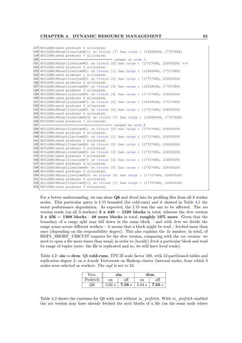
CHAPTER 4. DYNAMIC RESOURCE MANAGEMENT 65
117 BUILDER:send producer 6 allocated.118 BUILDER:MScan(lineitem@11) on thread [7] has range : [12648448, 17727488)119 BUILDER:send producer 7 allocated.120 ===================================== ranges on node 1121 BUILDER:MScan(lineitem@0) on thread [0] has range : [17727488, 22806528) ***122 BUILDER:send producer 0 allocated.123 BUILDER:MScan(lineitem@1) on thread [1] has range : [12648448, 17727488)124 BUILDER:send producer 1 allocated.125 BUILDER:MScan(lineitem@3) on thread [2] has range : [17727488, 22806528)126 BUILDER:send producer 2 allocated.127 BUILDER:MScan(lineitem@4) on thread [3] has range : [12648448, 17727488)128 BUILDER:send producer 3 allocated.129 BUILDER:MScan(lineitem@6) on thread [4] has range : [17727488, 22806528)130 BUILDER:send producer 4 allocated.131 BUILDER:MScan(lineitem@7) on thread [5] has range : [12648448, 17727488)132 BUILDER:send producer 5 allocated.133 BUILDER:MScan(lineitem@9) on thread [6] has range : [17727488, 22806528)134 BUILDER:send producer 6 allocated.135 BUILDER:MScan(lineitem@10) on thread [7] has range : [12648448, 17727488)136 BUILDER:send producer 7 allocated.137 ===================================== ranges on node 2138 BUILDER:MScan(lineitem@1) on thread [0] has range : [17727488, 22806528)139 BUILDER:send producer 0 allocated.140 BUILDER:MScan(lineitem@2) on thread [1] has range : [17727488, 22806528)141 BUILDER:send producer 1 allocated.142 BUILDER:MScan(lineitem@4) on thread [2] has range : [17727488, 22806528)143 BUILDER:send producer 2 allocated.144 BUILDER:MScan(lineitem@5) on thread [3] has range : [17727488, 22806528)145 BUILDER:send producer 3 allocated.146 BUILDER:MScan(lineitem@7) on thread [4] has range : [17727488, 22806528)147 BUILDER:send producer 4 allocated.148 BUILDER:MScan(lineitem@8) on thread [5] has range : [17727488, 22806528)149 BUILDER:send producer 5 allocated.150 BUILDER:MScan(lineitem@10) on thread [6] has range : [17727488, 22806528)151 BUILDER:send producer 6 allocated.152 BUILDER:MScan(lineitem@11) on thread [7] has range : [17727488, 22806528)153 BUILDER:send producer 7 allocated.
For a better understanding, we ran alone Q6 and dived into its profiling files from all 3 workernodes. This particular query is I/O bounded (for cold-runs) and it showed in Table 4.1 theworst performance degradation. As expected, the I/O was the one to be affected. The sinversion reads (on all 3 workers) 3 x 440 = 1320 blocks in total, whereas the drm version3 x 456 = 1368 blocks – 48 more blocks in total, roughly 10% more. Given that theboundary of a range split may fall down in the same block – and with drm we divide therange scans across different workers – it means that a block might be read / fetched more thanonce (depending on the responsibility degree). This also explains the 2x number, in total, ofHDFS_SHORT_CIRCUIT requests for the drm version, comparing with the sin version: weneed to open a file more times than usual, in order to (locally) fetch a particular block and readits range of tuples (note: the file is replicated and so, we still have local reads).
Table 4.2: sin vs drm: Q6 cold-runs, TPC-H scale factor 100, with 12-partitioned tables andreplication degree 2, on a 4-node Vectorwise on Hadoop cluster (internal nodes, from which 3nodes were selected as workers. The mpl is set to 24.
Vers. sin drmPrefetch on off on off
Q6 5.02 s 7.58 s 5.84 s 7.65 s
Table 4.2 shows the runtimes for Q6 with and without io_prefetch. With io_prefetch enabledthe sin version may have already fetched the next blocks of a file (on the same node where
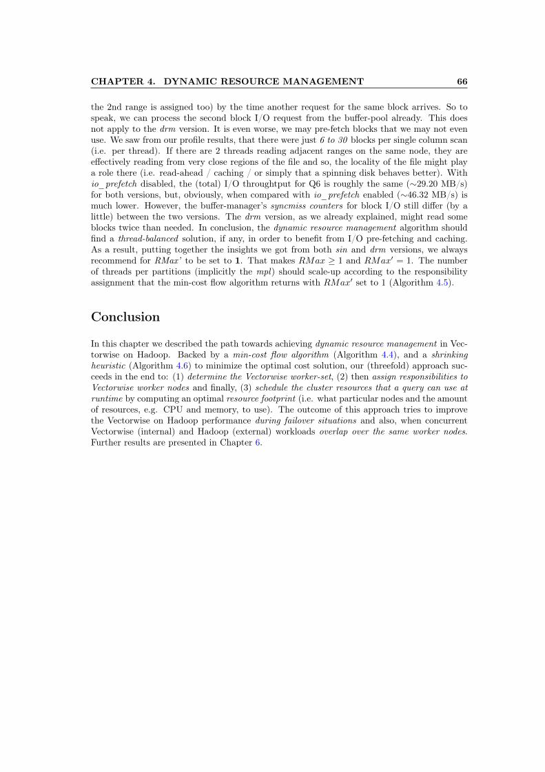
CHAPTER 4. DYNAMIC RESOURCE MANAGEMENT 66
the 2nd range is assigned too) by the time another request for the same block arrives. So tospeak, we can process the second block I/O request from the buffer-pool already. This doesnot apply to the drm version. It is even worse, we may pre-fetch blocks that we may not evenuse. We saw from our profile results, that there were just 6 to 30 blocks per single column scan(i.e. per thread). If there are 2 threads reading adjacent ranges on the same node, they areeffectively reading from very close regions of the file and so, the locality of the file might playa role there (i.e. read-ahead / caching / or simply that a spinning disk behaves better). Withio_prefetch disabled, the (total) I/O throughtput for Q6 is roughly the same (∼29.20 MB/s)for both versions, but, obviously, when compared with io_prefetch enabled (∼46.32 MB/s) ismuch lower. However, the buffer-manager’s syncmiss counters for block I/O still differ (by alittle) between the two versions. The drm version, as we already explained, might read someblocks twice than needed. In conclusion, the dynamic resource management algorithm shouldfind a thread-balanced solution, if any, in order to benefit from I/O pre-fetching and caching.As a result, putting together the insights we got from both sin and drm versions, we alwaysrecommend for RMax’ to be set to 1. That makes RMax ≥ 1 and RMax′ = 1. The numberof threads per partitions (implicitly the mpl) should scale-up according to the responsibilityassignment that the min-cost flow algorithm returns with RMax′ set to 1 (Algorithm 4.5).
Conclusion
In this chapter we described the path towards achieving dynamic resource management in Vec-torwise on Hadoop. Backed by a min-cost flow algorithm (Algorithm 4.4), and a shrinkingheuristic (Algorithm 4.6) to minimize the optimal cost solution, our (threefold) approach suc-ceeds in the end to: (1) determine the Vectorwise worker-set, (2) then assign responsibilities toVectorwise worker nodes and finally, (3) schedule the cluster resources that a query can use atruntime by computing an optimal resource footprint (i.e. what particular nodes and the amountof resources, e.g. CPU and memory, to use). The outcome of this approach tries to improvethe Vectorwise on Hadoop performance during failover situations and also, when concurrentVectorwise (internal) and Hadoop (external) workloads overlap over the same worker nodes.Further results are presented in Chapter 6.
Chapter 5
YARN integration
Today’s enterprises are looking to go beyond batch processing and integrate existing applicationswith Hadoop to realize the benefits of real-time processing and interactive query capabilities.As more organizations move from single-application Hadoop clusters to a versatile, integratedHadoop 2 data platform hosting multiple applications, YARN is positioned as the integrationpoint of today’s enterprise data layer. At the architectural center of Hadoop, YARN providesaccess to the main resources of the platform. Hence, any MPP database system, whose archi-tecture leverages the Hadoop capabilities and wishes to be a ’fair citizen’ of the ecosystem,should integrate with YARN.
Let us consider the following scenario: suppose we want a set of processes to co-exist withina Hadoop cluster. Furthermore, as requirement, these processes must run out-of-band fromYARN, which means that YARN is not allowed to control their life-cycle. These processes use,dynamically, different amounts of CPU and memory based on their load (we do not consideryet I/O or network bandwidth resource allocation since YARN does not support that). TheirCPU and memory requirements are managed independently from YARN. With other words,depending on their load, they might require more CPU but not more memory, or vice-versa.However, using YARN (Resource Manager) for scheduling out-of-band processes too, we shouldbe able to share and utilize appropriately (e.g. without contention) the compute resources ofan entire Hadoop cluster. Hence, we can let YARN be aware of all the allocated resourceswithin the cluster, whether they were needed for Hadoop jobs or some out-of-band workloads.The out-of-band processes must run a YARN Application Master (see Section 1.2.4) in orderto interact with YARN and negotiate for compute resources. When the Application Master isgranted with all it required, we bump up their CPUs and/or memory utilization. Though thisaction is "hidden" from YARN, we do make sure that our resource utilization is still withinthe granted limits. Whenever these processes back off, their allocation should also be releasedby YARN. Basically, we have to kill their Application Master(s). Using an approach like this,Hadoop’s running jobs and other out-of-band processes can fairly share the entire cluster’scompute resources. YARN would be the only one that does the resource bookkeeping. TheApplication Master should run in unmanaged mode (on any of the Haoop nodes) in order tozero out the necessity of allocating one container within YARN (in managed mode). To note,the latter option needs the minimum resource allocation per container as predefined in theconfiguration files. Once the Application Master runs, it will fork container processes at thecorresponding Node Managers to do nothing more than a basic sleep-forever.
67

CHAPTER 5. YARN INTEGRATION 68
5.1 Overview: model resource requests as separate YARNapplications
As we briefly explained in the beginning of this chapter, the approach to integrate Vectorwisewith YARN is to model resource requests as separate YARN (native) Applications. Implicitly,based on Section 1.2.4, every resource request will fork its own YARN Application Master.The idea is to focus towards allocating resources per workload instead of per query. It reducesthe number of resource requests (i.e. request latency) and also decreases the query’s runtimeoverhead. Starting a YARN Application Master means to request and allocate some set ofresources, reserve specific containers, run the container processes, and monitor the application’sstatus. Nonetheless, this usually comes with a big overhead: 5-7 seconds, depending on theResource Scheduler if it is busy or not. For instance, just to request and get some computeresources within YARN (w/o the other steps) it takes approx. 80% of the overhead time.And to do so per query, in which case we have to acquire before and release afterwards, istoo overwhelming. Instead, a per workload basis (coarse-grained) approach is more suitablefor a real-time integration. We see a Vectorwise workload as a group of queries with similarmaximum parallelism level and resource requirements that run on the same (sub)set of workersfor an unpredictable amount of time. From a workload management point of view, in time, theseworkloads will inevitable change the resource utilization of the Vectorwise database within theHadoop cluster. Hence, it is important for us to detect such events in order to know when torequest extra resources from YARN and achieve elasticity within the Hadoop ecosystem. To doso, we defined the notion of a system context. The system context refers to a moment in timewhen a query starts running on partitioned/non-partitioned tables and/or at the same time withother overlapping queries. Each time this context changes, e.g. one partitioned query startsrunning concurrently with a non-partitioned query, the (Vectorwise) resource manager willspan a different resource footprint during the query rewriting phase. We recommend reviewingSection 1.3.2 and 4.3 to remember how the previous steps work. If we can detect these changesin time we could know whether or not to request extra resources. For the moment, it iseasier to think of it as a 2-dimensional matrix system − context := [partitionedQuery ∈{true, false}][numQuery ∈ {1, . . . ,N}]← true, false from which we can remember if a contextchange actually occurred; at X100 bootstrap we initialize the matrix with false and reset it to thesame value when every query workload has ended. A Vectorwise workload is created when thefirst of its queries starts running in the system; a system context change is recorded and clusterresources get requested from YARN. It is assumed that, within the same workload, the latencybetween two consecutive queries is small. Therefore, we can imply that a Vectorwise workloadends when its latest query finishes and the duration of the idle (workload) state passes over acertain threshold (set by the user). If that happens, the approach takes a pessimistic decisionand ends the current workload by stopping its correspondent YARN Application Master. Thenext query will start a new workload and try to reclaim its resource footprint, though it isunfortunate when the query could have been related to the previous workload. However, queriesrunning in a different system context or with different resource requirements are treated asseparate workloads. If some workloads have to run concurrently, then the system will try toallocate more resources to fulfill both’s footprint requirements (but all within the cluster’smaximum capability). For implementation details we recommend reading Section 5.3.
Figure 5.1 illustrates an example of running multiple Vectorwise queries on 3 worker nodeswith 8 cores each [8, 8, 8], plus 0.25 maximum core over-allocation. We use various colors(green, purple, red) to differentiate between different workloads. Important to notice are thetwo scenarios explained above: (1) if the timeout exceeds, the next query starts a new workload(green color) and (2) different overlapping queries need extra resources, within the maximumcapabilities (green to purple to red, but not purple to violet). The example starts with a queryworkload (green color) that acquires [4, 4, 4] threads per node (mpl = 12 ). When it finished andthe idle_timeout have passed, we release those resources. Then, it happens that another query

CHAPTER 5. YARN INTEGRATION 69
(green color again), which could have been part of the previous workload, starts running in thesystem and targets the same resource footprint (mpl = 12 ). Since it starts after the idle_-timeout, it has to regain its amount of resources back from YARN. Next, we have a sequence ofthree queries: the first two queries (purple color) that are from the same workload, both askingfor [2, 2, 2] threads per node (mpl = 6 ) and the third one (red color) that overlaps with all theother queries/workloads aiming towards [4, 4, 4] threads per node (mpl = 12 ); for the thirdquery we need to use the 0.25 core over-allocation in order to achieve its mpl.
Figure 5.1: Timeline of different query workloads.
An overview of the approach is illustrated in Figure 5.2. Basically, the figure depicts a two-phase workflow. The integration starts with the Vectorwise worker-set initialization phase (P1),given that we previously decided the responsibility assignment. During this phase we allocatethrough YARN the initial amount of resources for the database to be operable, e.g. run dis-tributed queries w/o any parallelism, 1 core + enough memory for query execution and bufferpool per worker. This phase is managed by the WorkerSetInit component (custom YARNApplication Master). From this point on starts the second phase (P2). Any request to in-crease the worker-set amount of resources, i.e. extra CPU and memory to run a new workload,is sent directly to the DbAgent component (custom YARN ClientApplication). Besides whatis described in the previous chapters, the DbAgent is also responsible for resource allocationwithin YARN (i.e. to acquire or release new containers). For each request that it receives, itspawns a new YARN Application Master (IncreaseResources component) that negotiates withthe ResourceManager the demand for extra containers: it reserves and starts containers withspecific resource requirements on a subset of (or all) worker nodes and then it manages their life-cycle. Previously to any resource request, the Vectorwise Master node asks the DbAgent for thecurrent resource state of the cluster (e.g. available/used resources) in order to compute the re-source footprint of a new query workload. Both, the update worker-set state and acquire/releasesend-receive requests, are part of the DbAgent to Vectorwise Master communication protocol.More details will be given in Section 5.2 and Section 5.3.
Under the hood, the DbAgent uses a set of YARN Application Masters that run as unmanagedJVM processes, i.e. they run isolated from YARN and need no resource allocation in particular.Each one negotiates specific resource requirements with the Resource Manager, reserves andruns one container per worker node, and then loops around to manage their life cycle. We notethat, in our case, these containers do not run computational tasks as they should (e.g. as withMap-Reduce framework). Instead, the "placeholder" processes running inside the containers arejust monitoring the co-located X100 servers, on the same worker nodes (e.g. poking the serverto see if it is still alive). These processes run a while-check-sleep primitive and thus, their CPUand memory usage is negligible. The unmanaged YARN Application Master can be spawned byeither (1) an initial request to allocate the minimum amount of (CPU and memory) resourcesneeded to bootstrap Vectorwise and be operable to users (e.g. at least 1 core + enough memoryfor query execution per node) or (2) new resource requests for different (maybe overlapping)query workloads. Therefore, Vectorwise manages its own X100 back-end processes out-of-bandfrom YARN ; it uses YARN just for resource bookkeeping and for (Hadoop) cluster-awareness.

CHAPTER 5. YARN INTEGRATION 70
Figure 5.2: Out-of-band approach for Vectorwise-YARN integration. An example using 2 xHadoop nodes that equally share 4 x YARN containers.
The distribution of resources is completely managed by YARN and we just control the nodelocations (i.e. worker nodes) where our resources should be allocated.
As stated in YARN-896 1, there is significant work ongoing to allow long-lived services run-ning as YARN applications. For example, the API’s functionality to increase/decrease resourceutilization within YARN containers (YARN-1197 2) is not yet implemented. This makes itimpossible "per se" to gain full elasticity and to allocate/deallocate resources in a fine-grainedfashion for Vectorwise. Though the idea to model resource requests as separate YARN appli-cations achieves elasticity to a certain extent for increasing the amount of resources, we arelimited when it comes to the opposite operation, decreasing resources. To explain why, letus consider the following scenario: we assume to have the same 3 workers with 8 cores each,but 2 queries running at the same time. If the first query needs all 24 available cores (mpl= 24 gets all the 3 workers), the other would get only 10 cores; the second query’s mpl islimited to 16 threads max+16∗0.25 over−allocation
2 queries = 10 threads. We reference Section 1.3.3 for thetwo (before-mentioned) scheduling policies and recommend reviewing Section 5.1 to understandwhat comes next. Assuming the two queries as being part of different workloads, e.g. first queryruns on partitioned data and the second not, the first workload would then allocate the amountof resources it needs before it starts. On the other hand, the second workload does nothingbecause the available cores are all claimed already. At this moment, just one YARN ApplicationMaster (for the first workload) negotiates the resource footprint and manages the 3 placeholderprocesses (one per node). When both queries are still active or the second one finishes faster,that is fine. The problem appears if the first workload finishes earlier and we have to stop itsYARN Application Master to release the amount of allocated resources (i.e. all cores). More-over, this means to leave the second query (using 10 cores) running, but "outside" YARN /
1YARN-896: issues.apache.org/jira/browse/YARN-8962YARN-1197: issues.apache.org/jira/browse/YARN-1197

CHAPTER 5. YARN INTEGRATION 71
without resource-bookkeeping. Besides, we cannot just deallocate the difference of resourcesbetween the first and second workload using the available API interface. With the existingYARN version this functionality can be translated into (1) stopping the existent ApplicationMaster (for the first query) and then (2) starting another one (for the second query), whichadds a significant overhead and is not a worthwhile solution to implement (from a product-wisepoint of view). Therefore, our workaround is to release all requested resources at once, whenthe latest workload ends (idle state duration > threshold) and there are no other queries stillactive in the system. What is changed from Figure 5.1 is shown below, in Figure 5.3.
Figure 5.3: Timeline of different query workloads (one-time release).
However, as YARN-1197 is being pushed for the next release version of YARN, we are going torevise this approach in the near future. For instance, instead of creating one YARN ApplicationMaster per resource request (per workload), we could multiplex all the requests towards a singleYARN application (or a pool of applications distributed over different scheduling queues) thatdynamically increases/decreases its containers’ amount of resources. Thereby we can avoid theapplication startup overhead entirely and reduce the request latency even more (i.e. a YARNApplication Master can run in background and listen only for new requests).
Another alternative is to use Apache’s Slider 1 platform, launched in beta-version around June2014, which exposes a set of services that allow long-running applications, real-time and onlineapplications to easily integrate into YARN (and be YARN-Ready 2). Besides, it provides aninterface for real-time communication, especially for database systems running on Hadoop ordatabase-style workloads where a very high-speed transfer or data processing and responsetimes are required. It complements Apache Tez 3, which is quickly gaining adoption as thebatch and interactive engine of Hadoop. However, one thing to note, is that Slider, as well asthe YARN 2.2 release, do not support resource extension (i.e. increase or decrease primitives)for containers yet. This means we would still need a work-around to achieve resource elasticityfor Vectorwise on Hadoop, to allocate or deallocate resources when is required so.
1Apache Slider: slider.incubator.apache.org2YARN-Ready Program: hortonworks.com/press-releases/hortonworks-announces-yarn-ready-program3Apache Tez: tez.apache.org
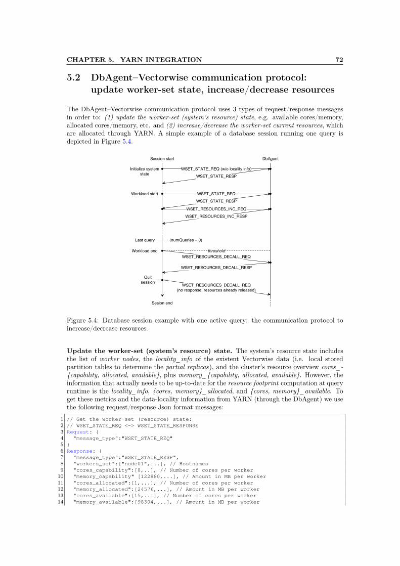
CHAPTER 5. YARN INTEGRATION 72
5.2 DbAgent–Vectorwise communication protocol:update worker-set state, increase/decrease resources
The DbAgent–Vectorwise communication protocol uses 3 types of request/response messagesin order to: (1) update the worker-set (system’s resource) state, e.g. available cores/memory,allocated cores/memory, etc. and (2) increase/decrease the worker-set current resources, whichare allocated through YARN. A simple example of a database session running one query isdepicted in Figure 5.4.
Figure 5.4: Database session example with one active query: the communication protocol toincrease/decrease resources.
Update the worker-set (system’s resource) state. The system’s resource state includesthe list of worker nodes, the locality_info of the existent Vectorwise data (i.e. local storedpartition tables to determine the partial replicas), and the cluster’s resource overview cores_-{capability, allocated, available}, plus memory_{capability, allocated, available}. However, theinformation that actually needs to be up-to-date for the resource footprint computation at queryruntime is the locality_info, {cores, memory}_allocated, and {cores, memory}_available. Toget these metrics and the data-locality information from YARN (through the DbAgent) we usethe following request/response Json format messages:
1 // Get the worker-set (resource) state:2 // WSET_STATE_REQ <-> WSET_STATE_RESPONSE3 Request: {4 "message_type":"WSET_STATE_REQ"5 }6 Response: {7 "message_type":"WSET_STATE_RESP",8 "workers_set":["node01",...], // Hostnames9 "cores_capability":[8,..], // Number of cores per worker
10 "memory_capability" [122880,...], // Amount in MB per worker11 "cores_allocated":[1,...], // Number of cores per worker12 "memory_allocated":[24576,...], // Amount in MB per worker13 "cores_available":[15,...], // Number of cores per worker14 "memory_available":[98304,...], // Amount in MB per worker

CHAPTER 5. YARN INTEGRATION 73
15 "locality_info":{16 "partition-id":[local-nodes,...], // Workers location17 ...18 }19 }
Increase/decrease the amount of resources. To increase the current amount of resourceswe specify into a Json format message how many extra cores and memory we need per node,depending on the resource footprint’s specification. To decrease them we just send a requestto the DbAgent at the end of the latest query workload (after the idle_timeout threshold) andeverything will go back to the initial resource state (i.e. as it was at startup).
1 // Increase worker-set resources:2 // WSET_RESOURCES_INC_REQ <-> WSET_RESOURCES_INC_RESP3 Request: {4 "message_type":"WSET_RESOURCES_INC_REQ",5 "cores_plus":[15,...], // Number of cores per worker6 "memory_plus":[98304,...] // Amount in MB per worker7 }8 Response: {9 "message_type":"WSET_RESOURCES_INC_RESP",
10 "response":"SUCCEEDED"|"FAILED"11 }12 // Decrease worker-set resources:13 // WSET_RESOURCES_DECALL_REQ <-> WSET_RESOURCES_DECALL_RESP14 Request: {15 "message_type":"WSET_RESOURCES_DECALL_REQ",16 }17 Response: {18 "message_type":"WSET_RESOURCES_DECALL_RESP",19 "response":"SUCCEEDED"|"FAILED"20 }
5.3 Workload monitor & resource allocation
For resource allocation within YARN we make use of the query’s resource footprint (work-ersSubset, responsibilities, maximum threads per worker) tuple, which implicitly contains in-formation on how many threads per worker node need to be claimed (in total) for a queryat runtime. Based on the communication protocol from Section 5.2, when we request ex-tra resources (from the Resource Manager) for a workload the idea is to fill-out the cores_-plus:[...] list from the message-body with the difference between the maximum threads perworker (member of the footprint tuple) and the current state of the allocated resources:footprint.maximumThreadsPerWorker−allocatedCores (1 thread : 1 core). In other words,the resource footprint tells us how many cores/threads we need more when compared to thecurrent state of the system. Obviously, if the difference is negative then extra resources arenot available for the moment and we should not even try to send a request to increase those.However, we record this "failure" in the system such that, after a system config failure_timeout,another query from the same workload tries again to acquire from YARN what was previouslyneeded. The workload monitor’s and resource allocation’s workflow is illustrated in Figure 5.5.The figure depicts two possible scenarios: (a) when the resource request was successfully , be-ing able to acquire the resource footprint, and (b) if it failed because of an external (Hadoop)workload overlapping on the same set of resources. For both, we show in particular (usingdistinct colors) what is the YARN footprint at each step, for (a) on left and (b) on right.Following the workflow’s state transitions (from left to right) the reader can notice that the first4 steps (enter, attempt on (YARN) resources, compute the resource footprint and acquire exactresources) are common to all query workloads. A "branch-out" may happen after a resource

CHAPTER 5. YARN INTEGRATION 74
request is sent to the DbAgent. Depending on the resource availability within the Hadoop clus-ter, the request can either succeed, case in which we update (green color) the system state tothe current level of allocated resources, or fail because of a situation with no more availableresources (e.g. overlapping external workloads). For the latter we should rollback (red color) tothe previous system state (i.e. to what resources were available before the attempt) and recordthis "failure" (light blue color). For (a) we release the workload’s extra resources when thisends (and the idle_timeout is passed), whereas for (b) we do not have to release anything. Yet,we do have to retry (light blue color) to obtain our resources after a certain time; typically this"waiting" time is equal with the before mentioned failure_timeout.
Figure 5.5: The workload monitor’s and resource allocation’s workflow for: a) successful(resource) request and b) failed (resource) request (VW – Vectorwise, MR – Map-Reduce)
Omitted from the resource footprint are the memory requirements, which are computed sep-arately from the resource scheduler’s implementation. The standard way of specifying theamount of memory for Vectorwise is by setting static values for the buffer pool and query ex-ecution memories inside the configuration file. Since the buffer pool is relatively independentfrom the query execution, there is no relation as such to allow us increasing its memory sizedynamically at query runtime. Therefore, this value is read from the configuration file andset as a X100 initialization argument in the worker-set startup command; initial resources areallocated from YARN before running the X100 (worker-set) backend processes. For query ex-ecution we defined a linear function to increase the memory size at runtime; the total amountto increase is proportionally to the footprint’s demand of core/thread resources and is limitedby the (maximum) available memory on each of the worker nodes.
The implementation of the resource allocation functionality follows the approach described inSection 5.1, a per workload resource allocation with a one-time release, and uses the communi-cation protocol from Section 5.2 to update/acquire/release resources. A high-level pseudocode ofthe runtime resource allocation routine is presented in Algorithm 5.1. Algorithm 5.2 shows thepseudocode implementation of the update/acquire/release primitives. In addition, the workloadmonitor uses a thread to monitor the workload’s start/stop state changes and also to simulatethe system’s idle state, knowing when to release the extra amount of resources. The monitor-ing thread is created during the system’s initialization phase, starts measuring the idle stateeach time the latest query workload (i.e. numQueries=0 ) leaves Vectorwise and it stops whenthe duration of the idle state passes a certain threshold (or idle timeout) configured by theuser. When this thread stops, a request to release all resources is sent to the DbAgent. Thepsuedocode implementation of the workload monitor’s functions is given in Algorithm 5.3.

CHAPTER 5. YARN INTEGRATION 75
Algorithm 5.1 High-level pseudocode: workload-monitor & resource allocation
partitioned ∈ {true, false}numQueries ∈ {1 . . .N}
1: (1) Query Enter2: numQueries← numQueries+ 13: stopT imeoutThread()4: . . .5: (2) In Rewriter Phase: inside the parallel rule where the footprint
and the feasible solution are computed6: attemptIncrease ← attemptIncreaseResources(partitioned, numQueries) // update the
system’s state with all the available resources from YARN7: do8: rollback ← false9: // if attemptIncrease is true, it means that the system’s state is updated "temporarily" with the
resource information we get from YARN (e.g. allocated resources, available/extra resources, etc.)10: footprint← footprint(...) // is the resource scheduler’s job to compute the current footprint
11: if attemptIncrease ∧ ¬acquireExtraResources(footprint, partitioned, numQueries)12: rollback ← true13: rollbackSystemState()14: attemptIncrease← false15: end if16: while rollback17: if attemptIncrease then18: // make the attempt consistent with the sate of the system19: updateSystemState(footprint)20: else21: // (1) the attempt failed, or (2) there were not enough available resource at the moment22: checkSystemState(partitioned, numQueries, footprint) // check if the system is underprovi-
sioned23: end if24: . . .25: (3) Query Exit26: numQueries← numQueries− 127: if numQueries = 0 then28: startT imeoutThread()29: end if
The above high-level pseudocode, Algorithm 5.1, introduces the resource allocation at queryruntime and it complies with Figure 5.5, the logical workflow of the resource allocation andworkload monitor. When a query enters the system we increase the number of active queriesand stop the workload monitor from its sleeping-condition that simulates the idle state, lines 2and 3. From line 6 to 24 is the runtime resource allocation routine: we make an attempt over allYARN’s available resource and we try to acquire the current resource footprint’s requirements.If the request failed we fall into a rollback procedure in which we change the system’s stateto the previous state and recompute the resource footprint ; mpl should be decreased if thathappens. However, during the checkSystemState(. . .) function at line 22 will make sure that,after a certain failed_timeout time, a next query from the same workload is going to try againand acquire what resources were needed initially. Last but not least, when a query exits thesystem we decrease the number of active queries and if there are no others we can start theworkload monitor, lines 27 to 30.
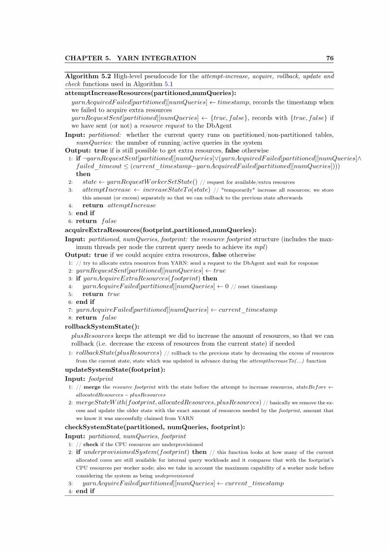
CHAPTER 5. YARN INTEGRATION 76
Algorithm 5.2 High-level pseudocode for the attempt-increase, acquire, rollback, update andcheck functions used in Algorithm 5.1attemptIncreaseResources(partitioned,numQueries):yarnAcquiredFailed[partitioned][numQueries]← timestamp, records the timestamp whenwe failed to acquire extra resourcesyarnRequestSent[partitioned][numQueries] ← {true, false}, records with {true, false} ifwe have sent (or not) a resource request to the DbAgent
Input: partitioned: whether the current query runs on partitioned/non-partitioned tables,numQueries: the number of running/active queries in the system
Output: true if is still possible to get extra resources, false otherwise1: if ¬yarnRequestSent[partitioned][numQueries]∨(yarnAcquiredFailed[partitioned][numQueries]∧
failed_timeout ≤ (current_timestamp−yarnAcquiredFailed[partitioned][numQueries])))then
2: state← yarnRequestWorkerSetState() // request for available/extra resources3: attemptIncrease ← increaseStateTo(state) // "temporarily" increase all resources; we store
this amount (or excess) separately so that we can rollback to the previous state afterwards4: return attemptIncrease5: end if6: return false
acquireExtraResources(footprint,partitioned,numQueries):Input: partitioned, numQueries, footprint: the resource footprint structure (includes the max-
imum threads per node the current query needs to achieve its mpl)Output: true if we could acquire extra resources, false otherwise1: // try to allocate extra resources from YARN: send a request to the DbAgent and wait for response2: yarnRequestSent[partitioned][numQueries]← true3: if yarnAcquireExtraResources(footprint) then4: yarnAcquireFailed[partitioned][numQueries]← 0 // reset timestamp5: return true6: end if7: yarnAcquireFailed[partitioned][numQueries]← current_timestamp8: return false
rollbackSystemState():plusResources keeps the attempt we did to increase the amount of resources, so that we canrollback (i.e. decrease the excess of resources from the current state) if needed
1: rollbackState(plusResources) // rollback to the previous state by decreasing the excess of resourcesfrom the current state, state which was updated in advance during the attemptIncreaseTo(...) function
updateSystemState(footprint):Input: footprint1: // merge the resource footprint with the state before the attempt to increase resources, stateBefore ←
allocatedResources− plusResources
2: mergeStateWith(footprint, allocatedResources, plusResources) // basically we remove the ex-cess and update the older state with the exact amount of resources needed by the footprint, amount thatwe know it was successfully claimed from YARN
checkSystemState(partitioned, numQueries, footprint):Input: partitioned, numQueries, footprint1: // check if the CPU resources are underprovisioned2: if underprovisionedSystem(footprint) then // this function looks at how many of the current
allocated cores are still available for internal query workloads and it compares that with the footprint’sCPU resources per worker node; also we take in account the maximum capability of a worker node beforeconsidering the system as being undeprovisioned
3: yarnAcquireFailed[partitioned][numQueries]← current_timestamp4: end if

CHAPTER 5. YARN INTEGRATION 77
Algorithm 5.3 High-level pseudocode for the workload-monitor’s run, start, stop, and exitfunctions used in Algorithm 5.1the timeoutThread checks whether all Vectorwise workloads have finished, so that we knowwhen to release the amount of extra resources; it starts running when the database sessionis initialized for the first timetimeoutThread.state ∈ {START, STOP,EXIT}, where START/STOP are related to theworkload’s IDLE/RUNNING states and EXIT is used when the system shuts down
runTimeoutThread():1: acquireLock()2: while ¬timeoutThread.state = EXIT do3: waitOnCondition(timeoutThread.condition, getLock())4: if ¬timeoutThread.state = EXIT then5: now ← currenttimestamp6: timedWaitOnCondition(timeoutThread.sleepCondition, getLock(), now +
idle_timeout) // simulate the idle-state: wait until the idle_timeout threshold is passed7: end if8: if timeoutThread.state = START then9: // release all resources
10: reinitializeSystem() // rollback to the initial (resource) state of the system11: yarnReleaseExtraResources() // send a WSET_RESOURCES_DECALL_REQ to the
DbAgent12: end if13: end while14: releaseLock()
startTimeoutThread():1: acquireLock()2: timeoutThread.state← START3: awake(timeoutThread.condition)4: releaseLock()
stopTimeoutThread():1: acquireLock()2: timeoutThread.state← STOP3: releaseLock()
exitTimeoutThread():1: acquireLock()2: timeoutThread.state← EXIT3: awake(timeoutThread.condition)4: awake(timeoutThread.sleepCondition)5: releaseLock()
Algorithm 5.2 brings up the attempt-increase, acquire, rollback, update and check func-tions, used at runtime by the X100 Master to allocate resources from YARN. TheattemptIncreaseResources(. . .) function temporarily updates the state of the system, lines 2and 3, with all the available YARN resources (if any) as an optimistic approach to achievethe query’s mpl. We note that some resource footprints may need less cores then all theavailable. Another important function is acquireExtraResources(. . .) in which we try to claimthe extra cores we need (from YARN), compared to the current allocated cores per workernodes. This is done by sending an increase request to the DbAgent, lines 3 to 6. Theprevious two functions use yarnRequestSent[..][..] and yarnAcquiredFailed[..][..] matrices toverify (at attemptIncreaseResources : line : 1) and record (at acquireExtraResources :lines : 2, 4, 7) if any requests for specific workloads were sent and, respectively, if they

CHAPTER 5. YARN INTEGRATION 78
failed due to resource unavailability (i.e. an external Hadoop workload got the availableresources in the meantime). In Algorithm 5.3 we depict the workload-monitor’s run, start,stop and exit primitives. Important to emphasize is the runT imeoutThread(. . .) function,called during the Master’s system initialization. This function simulates the workload’s idle-ness when the thread is set on START state, lines 4 to 7, and releases the amount ofresources afterwards if this state has not been changed to STOP. The rest of the pseu-docode is self-explanatory. Because of space limits, we leave the remaining utility func-tions, such as the yarnRequestWorkerSetState(. . .), yarnAcquireExtraResources(. . .) andyarnReleaseExtraResources() functions, which implement Section 5.2’s protocol in orderto update, request and release resources, or the increaseStateTo(. . .), mergeStateWith(. . .),rollbackState(. . .), underprovisionedSystem(. . .) and reinitializeSystem() system’s helperfunctions uncovered.
YARN resource allocation overhead
1 2 3 4 5 6 7 8 9 10 11 12 13 14 15 16 17 18 19 20 21 22
0
0.5
1
1.5
2
2.5
3
3.5
4
4.5
55.07
0.61
0.16
0.40.31
5 · 10−20.29
0.44
0.98
1.57
0.250.15
3.54
0.260.36
1.15
0.41
0.93
0.580.36
1.37
0.66
0.280.360.16
0.40.31
5 · 10−20.29
0.44
0.98
1.57
0.250.15
3.54
0.260.36
1.15
0.41
0.93
0.580.36
1.37
0.66
Tim
e(s)
base (YARN disabled) allocation overhead (YARN enabled)
Figure 5.6: YARN’s allocation overhead: TPC-H scale factor 100, 32 partitions, 8 "Stones"nodes, 128 mpl.
To measure YARN’s resource allocation overhead, i.e. negotiating resources and reserving/run-ning specific containers, in a mixed scenario of queries we have run a TPC-H scale factor 100(Lineitems and Orders 32-partitioned) on a 8 "Stones" cluster (see 2.5), of which all of themwere selected for the worker-set. We have initialized Vectorwise with 1 Core + 24 GB per

CHAPTER 5. YARN INTEGRATION 79
worker and the mpl was set to 128, the maximum amount of cores in the cluster. No otherexternal (Hadoop Map-Reduce) jobs were running at the same time on the cluster; experimentsusing Hadoop-busyness are shown in Chapter 6.
In our case, the first 2 queries from TPC-H can already be classified into 2 different workloads:Query-1 reading Lineitem that is partitioned and Query-2 running on Part, Partsupp, Supplier,Region, Nation non-partitioned tables. Hence, all the required resources are allocated at thebeginning of the benchmark’s run (during the first 2 queries’ run). Yet, the (resource allocation)overhead is still not negligible. Results are shown in Figure 5.6.
As we can see from Figure 5.6, when Query-1 starts, there is an overhead of 4.79s betweenthe two of the runs that is used (in the YARN enabled version) to allocate 15 more cores andthe rest of the available memory per worker node. On the other hand, Query-2 requests onlya worker-set (resource info) update given that there are no resources left in the cluster. Thelater adds an overhead of 0.25s at query runtime.
Conclusion
In conclusion, we have shown how one can achieve resource elasticity for Vectorwise on Hadoop,alongside with the dynamic resource management described in the previous chapter, Chapter 4.Our approach to allocate resources per workload, instead of per query, and deallocate at oncewhen no query has been active for an idle_timeout reduces the overall overhead of resourcemanagement through YARN; the current’s YARN API release version adds a big overheadwhen starting an Application Master to negotiate resources and manage containers, Figure 5.6.However, as we explained in Section 5.1, we expect the previous issue to be fixed by the codecommit of YARN-1197 1 such that we could improve our approach and gain more elasticity inthe near future.
1YARN-1197: issues.apache.org/jira/browse/YARN-1197

Chapter 6
Evaluation & Results
6.1 Evaluation Plan
We have divided the evaluation of our research project in three separate phases, following theorder of which the project’s approach was presented with technical details throughout this thesis(in Chapter 3, Chapter 4, and Chapter 5):
• P1: HDFS custom block-placement policy
– Testing the HDFS custom block replication, which replicates and collocates Vec-torwise data, during a system fail-over (i.e. a node crash).
• P2: Dynamic resource scheduling algorithm
– Testing the min-cost flow (implicitly the cost-model) approach for reliability andperformance during node failovers.
** When a node fails the database session must be restarted and thus the buffer poolwill be empty. In this case, Vectorwise needs to access the HDFS layer in order to readits data.
• P3: YARN integration
– Testing the min-cost flow (implicitly the cost-model) approach while running otherexternal (Hadoop Map-Reduce) jobs on the same cluster nodes (i.e. simulating Hadoopbusyness).
We expect from each evaluation phase to derive the following conclusions:
• P1: The runtime performance should not degrade after data recovery. At the end of theHDFS data re-replication process, all missing replicas must be replicated and collocatedon the new worker nodes (or the remaining workers). The system’s I/O throughput inthis situation should be at least as it was during the cluster’s "healthy" state.
• P2: We achieve a better runtime performance (or at least the same as the baseline) byfavoring local reads vs remote (over TCP) reads.
• P3: We achieve a better runtime performance (and resource utilization) by steering theVectorwise query computation to the least loaded workers, with respect to their data-locality. Before running a query workload, we should have allocated the workload’s re-source footprint through YARN in order to reduce the resource contention.
80

CHAPTER 6. EVALUATION & RESULTS 81
Experimental Setup
All the experiments we present in this section were carried out on the available clusters ofcomputers that were described in Section 2.5. Table 6.1 shows the exact values we used for therelevant configuration parameters of Vectorwise on Hadoop (X100 engine).
Parameters Description Valuevector_size Processing unit size: the (maximum) number of
tuples returned by an operator’s next() method.1024
num_cores Number of available cores, depending on the cho-sen cluster to test.
4 or 16
bufferpool_size The amount of memory the I/O buffers can useto cache data from disk, depending on the chosencluster to test.
10GB or 48GB
num_recv_buf Number of buffers a DXchg Receiver uses to storeincoming messages.
2
num_send_buf Number of buffers per destination used by a DX-chg Sender.
2
max_xchg_buf_size The maximum size of the Xchg buffers, also usedas the fixed size of DXchg buffers (MPI messages).
256KB
thread_weight The weight of the thread load (wt, see Sec-tion 1.3.2)
0.3
enable_profiling Flag specifying whether detailed per-query profil-ing information should be collected.
TRUE
Table 6.1: Parameters configuration values
Both P1 and P2 try to highlight the importance of data locality in a system that suffers froma fail-over. Hence, we perform our tests on so-called "cold" I/O buffers (i.e. empty buffer pool,or cache). At the beginning of each test we clear the OS File System’s cache and before eachquery we use the X100’s clear_bm syscall to empty the I/O buffers.
On the other hand, P3’s goal is to emphasize the benefits of dynamic resource managementthrough YARN and is performed on "hot" I/O buffers. This means that MScan operators willalways read data from memory and there is no disk access whatsoever. As such, before runningany tests, we performed prior cold-runs (w/o calling the clear_bm syscall beforehand) to ensureall the required data would be available in the I/O buffers. We allowed each of the worker nodesused for testing to store up to its maximum buffer pool size of data. Since P3 requires morecomputation power because of the concurrent (Vectorwise) internal and (Hadoop Map-Reduce)external workloads, for this particular phase we used the more powerful "Stones" cluster nodes.
We note that only queries expressed in the Vectorwise algebra were used and, therefore, justthe X100 engine was put under stress. Nevertheless, since our solution does not modify the wayIngres interacts with the Vectorwise (X100) Master, there should be no issues regarding howIngres parses the SQL statements and sends the optimized X100 query plans.
The TPC-H Benchmark
For assessing the performance of our solution, we used the same benchmark according to whichthe non-distributed, commercial version of Vectorwise is usually evaluated internally, namelythe TPC-H benchmark 1, which simulates a real-world workload for large scale decision-supportapplications that is designed to have broad industry-wide relevance. This benchmark is designed
1www.tpc.org/tpch

CHAPTER 6. EVALUATION & RESULTS 82
and maintained by the Transaction Processing Performance Council and comes with a datagenerator and a suite of business oriented ad-hoc queries and concurrent data modifications.
The size of the data warehouse to be generated can be controlled by a parameter called ScaleFactor (SF). For our tests we used SF 100 and SF 300, which produce approximately 32GB and96GB of compressed data respectively. Order and Linitem are the only partitioned tables, 16or 32 partitions. We disabled the concurrent data modifications, as they are not yet supportedin our system, but executed all the 22 read-only SQL queries provided (for which the reader isreferred to the TPC-H website) for P1, P2 and just a subset of them, a workload composed ofQ1 and Q13, for P3. The two of the queries target opposite characteristics of the system, Q1being I/O bounded for cold-runs and CPU bounded for hot-runs, whereas Q13 is both networkand CPU bounded in the latter case (because of the big Join/DXchgHashSplit between Ordersand Customer tables and the afterwards Aggregations).
Simulating Hadoop Busyness
For testing how the min-cost flow (implicitly the cost-model) approach behaves while runningexternal workloads that overlap with the Vectorwise worker-set, we used the TeraSort 1 standardMapReduce sorting benchmark and ran different sort of jobs. TeraSort is a benchmark thatcombines testing the HDFS and MapReduce layers of a Hadoop cluster. As such it is notsurprising that this benchmark suite is often used in practice 2, which has the added benefitthat it allows people – among other things – to compare the results of their own cluster with theclusters of others. One can use the TeraSort benchmark, for instance, to iron out his Hadoopconfiguration. Typical areas where it is helpful, is to determine whether the resource containerassignments are sound (as they depend on the variables such as the number of cores per nodeand the available memory), whether other MapReduce-related parameters are set properly, orwhether the FairScheduler configuration someone came up with really behaves as expected.For us, TeraSort simulates Hadoop busyness in the cluster. We use this benchmark especiallyfor its the Map phase, which takes about 40% of the runtime and generates (for bigger datasets) a CPU avg. load of 80-90%. More details about our busyness workloads are given inTable 6.2. To make it even more interesting, we have configured our jobs to run either onthe full worker-set (8 nodes, not. full-set) or on the half of it (4 nodes, not. half-set). Thismakes the workload’s Map phase to be CPU and I/O intensive, respectively CPU and networkintensive (since Hadoop does not always match all Mappers with their right data-locality andneeds remote data access). Previously, we loaded our (5GB, 10GB and 100GB) data sets intwo directories, each one for its own full-set (loaded on 8 nodes) or half-set (loaded on 4 nodes)run.
Table 6.2: Workload runtime and CPU avg./peak load for TeraSort benchmark runs on differentdata-set sizes, number of Mappers/Reducers and node sets.
Busyness Full-set Half-setConfig. 596.8MB x 8w 1.2GB x 8w 11.6GB x 8w 1.2GB x 4w 2.4GB x 4w 23.3GB x 4w
16M/16R 35 s 56 s 461 s 108 s 207 s 1613 s32M/32R 30 s 43 s 266 s 63 s 112 s 628 s64M/64R 26 s 36 s 218 s 40 s 57 s 376 sCPU load 40− 50% 60− 70% 70− 80% 30− 40% 50− 60% 70− 80%CPU peak – – – – 80% 95%
1TeraSort package: hadoop.apache.org/docs/current/api/org/apache/hadoop/examples/terasort/package-summary.html
2TeraSort competition: sortbenchmark.org

CHAPTER 6. EVALUATION & RESULTS 83
6.2 Results Discussion
Instrumenting Block Replication
In Section 2.1 we have discussed the two of the HDFS local read options, through DataNode(out-of-box DataTransferProtocol) and direct local reads (short-circuit config), showing theresults of a performance comparison using the Test-DFS I/O benchmark in Table 2.1. Giventhat, it make sense to enable the short-circuit configuration during the cold-run tests and benefitfrom "real" data locality. We prove the later by running now a TPC-H cold-run on 8 "Rocks"workers with 32 mpl. As we can see from Figure 6.1, the overhead of sending data throughTCP sockets (though the data is stored locally) increases the individual query execution timeby 50% to 100% in some cases. The average I/O throughput per query drops down as well,Figure 6.3 (w/ block collocation enabled), from 31.81 MB/s to 21.65 MB/s.
1 2 3 4 5 6 7 8 9 10 11 12 13 14 15 16 17 18 19 20 21 22
0
5
10
15
20
25
30
35
40
45
50
26.05
18.42
3.791.75
4.672.86
10.7710.8
47.73
35.48
10.61
4.2
18.7
1.62.23
7.77
19.6
23.84
19.8217.74
12.51
5.05
17.6215.8
1.941.052.09
0.12
3.623.56
25.1427.12
8.57
1.54
13.57
0.660.9
6.31
1.53
9.02
3.29
10.02
3.43.01
Tim
e(s)
w/ short-circuit (Total: 159.88s)w/o short-circuit (Total: 304.89s)
Figure 6.1: Running with (w/) and without (w/o) short-circuit when block colloc. is enabled.TPC-H benchmark: 16-partitions for Order and Lineitem, 8 "Rocks" workers, 32 mpl.
Focusing on how we can instrument HDFS block replication, Chapter 3 describes our CustomBlock Placement Policy implementation for Vectorwise on Hadoop. At the end it also embodiessome preliminary results (Tables 3.1 and 3.2 and Figure 3.3) showing the benefits of this policywhile running just a sub-set of the TPC-H queries (1, 4, 6, and 12). Based on the preliminaryresults, we concluded that our custom policy is better (by 1.58-1.78x) than the default HDFSplacement after re-replication, having control over data (co)locality to worker nodes, whereasthe default behavior performs better during node failures (1.14-1.41x), due to new workernodes (replacing the failed ones) having some of the local data that Vectorwise queries mayneed. To strengthen this conclusion, we have extended the same test to all TPC-H queries.New results are described in the remaining of this section. Some of the results consider thecase when the entire cluster’s size is restricted to the exact number of Vectorwise workers (not.workers/hadoop-nodes(total-nodes) = 8/8(10)) to point out the consequences of limiting thedefault replication just to the current worker-set.
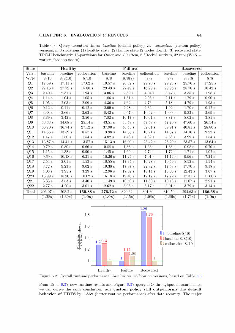
CHAPTER 6. EVALUATION & RESULTS 84
Table 6.3: Query execution times: baseline (default policy) vs. collocation (custom policy)versions, in 3 situations (1) healthy state, (2) failure state (2 nodes down), (3) recovered state.TPC-H benchmark: 16-partitions for Order and Lineitem, 8 "Rocks" workers, 32 mpl (W/N =workers/hadoop-nodes).
State Healthy Failure RecoveredVers. baseline baseline collocation baseline baseline collocation baseline baseline collocationW/N 8/10 8/8(10) 8/10 8/8 8/8(8) 8/8 8/8 8/8(8) 8/8Q1 17.59 s 17.11 s 17.62 s 19.57 s 26.32 s 29.70 s 29.23 s 25.76 s 17.25 sQ2 27.16 s 27.72 s 15.80 s 29.43 s 27.49 s 16.29 s 29.96 s 25.70 s 16.42 sQ3 2.40 s 2.31 s 1.94 s 3.06 s 2.89 s 4.04 s 3.47 s 3.35 s 1.98 sQ4 1.14 s 1.04 s 1.05 s 1.86 s 1.51 s 2.06 s 2.11 s 1.79 s 0.90 sQ5 1.95 s 2.03 s 2.09 s 4.36 s 4.62 s 4.76 s 5.18 s 4.79 s 1.93 sQ6 0.12 s 0.11 s 0.12 s 2.09 s 2.28 s 2.32 s 1.92 s 1.70 s 0.12 sQ7 3.38 s 3.66 s 3.62 s 8.42 s 9.67 s 10.42 s 10.33 s 9.32 s 3.69 sQ8 3.39 s 3.42 s 3.56 s 7.82 s 10.17 s 10.01 s 8.87 s 8.62 s 3.85 sQ9 33.33 s 34.08 s 25.14 s 43.51 s 53.48 s 47.48 s 47.70 s 47.60 s 26.54 sQ10 36.70 s 36.74 s 27.12 s 37.90 s 46.43 s 32.61 s 39.91 s 40.81 s 28.80 sQ11 14.56 s 13.59 s 8.57 s 13.98 s 14.38 s 10.21 s 14.37 s 14.16 s 9.22 sQ12 1.47 s 1.50 s 1.54 s 3.82 s 4.43 s 4.32 s 4.68 s 3.99 s 1.54 sQ13 13.87 s 14.41 s 13.57 s 15.13 s 16.00 s 23.42 s 26.29 s 23.57 s 13.64 sQ14 0.79 s 0.80 s 0.66 s 0.88 s 1.33 s 1.63 s 1.33 s 0.98 s 0.70 sQ15 1.15 s 1.38 s 0.90 s 1.45 s 1.69 s 2.74 s 1.72 s 1.71 s 1.02 sQ16 9.69 s 10.18 s 6.31 s 10.26 s 11.24 s 7.91 s 11.14 s 9.96 s 7.24 sQ17 2.54 s 2.01 s 1.53 s 10.55 s 17.34 s 16.28 s 10.59 s 8.52 s 1.54 sQ18 8.72 s 9.23 s 9.02 s 19.38 s 17.97 s 22.82 s 17.58 s 17.70 s 9.18 sQ19 4.03 s 3.95 s 3.29 s 12.96 s 17.62 s 18.14 s 13.05 s 12.43 s 3.67 sQ20 15.99 s 15.20 s 10.02 s 16.18 s 19.40 s 17.17 s 17.72 s 17.31 s 11.60 sQ21 3.33 s 3.53 s 3.40 s 11.49 s 10.50 s 11.80 s 10.43 s 11.07 s 2.91 sQ22 2.77 s 4.20 s 3.01 s 2.62 s 3.95 s 5.17 s 3.01 s 3.79 s 3.14 sTotal 206.07 s 208.2 s 159.88 s 276.72 s 320.62 s 301.30 s 310.59 s 294.63 s 166.68 s
(1.28x) (1.30x) (1.0x) (1.0x) (1.15x) (1.08x) (1.86x) (1.76x) (1.0x)
Healthy Failure Recovered
1
1.2
1.4
1.6
1.8
1.28
1
1.86
1.3
1.15
1.76
11.08
1
Tota
ltim
eM
IN
tim
eslow
er
baseline-8/10baseline-8/8(10)collocation-8/10
Figure 6.2: Overall runtime performance: baseline vs. collocation versions, based on Table 6.3
From Table 6.3’s new runtime results and Figure 6.3’s query I/O throughput measurements,we can derive the same conclusion: our custom policy still outperforms the defaultbehavior of HDFS by 1.86x (better runtime performance) after data recovery. The major
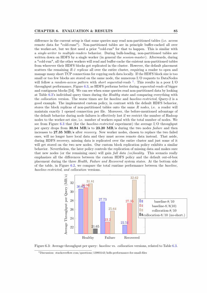
CHAPTER 6. EVALUATION & RESULTS 85
difference in the current setup is that some queries may read non-partitioned tables (i.e. accessremote data for "cold-runs"). Non-partitioned tables are in principle buffer-cached all overthe worker-set, but we first need a prior "cold-run" for that to happen. This is similar witha single-writer to multiple-readers behavior. During bulk-loading, non-partitioned tables arewritten down on HDFS by a single worker (in general the session-master). Afterwards, duringa "cold-run", all the other workers will read and buffer-cache the existent non-partitioned tablesfrom wherever their HDFS blocks got replicated in the cluster. However, the default placementscatters the remaining R-1 replicas all over the entire cluster, requiring a reader to open andmanage many short TCP connections for copying such data locally. If the HDFS block size is toosmall or too few blocks are stored on the same node, the numerous I/O requests to DataNodeswill follow a random-access pattern with short sequential-reads 1. This results in a poor I/Othroughput performance, Figure 6.3, as HDFS performs better during sequential-reads of biggerand contiguous blocks [54]. We can see when some queries read non-partitioned data by lookingat Table 6.3’s individual query times during the Healthy state and comparing everything withthe collocation version. The worse times are for baseline and baseline-restricted, Query-2 is agood example. The implemented custom policy, in contrast with the default HDFS behavior,stores the block replicas of non-partitioned tables onto the same R nodes, i.e. a reader willmaintain exactly 1 opened connection per file. Moreover, the before-mentioned advantage ofthe default behavior during node failures is effectively lost if we restrict the number of Hadoopnodes to the worker-set size, i.e. number of workers equal with the total number of nodes. Wesee from Figure 6.3 that (for the baseline-restricted experiment) the average I/O throughputper query drops from 30.94 MB/s to 23.20 MB/s during the two nodes failure and thenincreases to 27.35 MB/s after recovery. New worker nodes, chosen to replace the two failedones, will no longer have local data and they must access remote data instead. That aside,during HDFS recovery, missing data is replicated over the entire cluster and just some of itwill get stored on the two new nodes. Our custom block replication policy exhibits a similarbehavior. Nevertheless, the later policy controls the replication of missing data and makes surethat new nodes (or the remaining ones) will gain full data (co)locality. This scenario reallyemphasizes all the differences between the custom HDFS policy and the default out-of-boxplacement during the three Health, Failure and Recovered system states. At the bottom sideof the table, in Figure 6.2, we compare the total runtime performance between the baseline,baseline-restricted, and collocation versions.
Healthy Failure Recovered
22
24
26
28
30
3230.63
27.73
22.51
30.94
23.2
27.35
31.81
25.64
32.62
21.65
Average
Throu
ghpu
tpe
rQuery
(MB/s)
baseline-8/10baseline-8/8(10)collocation-8/10
collocation-8/10 (no-short.)
Figure 6.3: Average throughput per query: baseline vs. collocation versions, related to Table 6.3.
1Discussion: stackoverflow.com/questions/13993143/hdfs-performance-for-small-files

CHAPTER 6. EVALUATION & RESULTS 86
Table 6.4: Query execution times: baseline (default policy) vs. collocation (custom policy)versions, in 3 situations (1) healthy state, (2) failure state (2 nodes down), (3) recovered state.TPC-H benchmark: 32-partitions for Order and Lineitem, 8 "Rocks" workers, 32 mpl (W/N =workers/hadoop-nodes).
State Healthy Failure RecoveredVers. baseline collocation baseline collocation baseline collocationW/N 8/10 8/10 8/8 8/8 8/8 8/8Q1 19.13 s 19.91 s 20.88 s 22.86 s 25.78 s 18.66 sQ2 32.84 s 18.27 s 32.13 s 22.91 s 28.80 s 18.48 sQ3 3.01 s 2.74 s 3.47 s 4.05 s 4.13 s 2.91 sQ4 1.84 s 1.70 s 2.21 s 3.30 s 2.71 s 1.63 sQ5 1.94 s 1.77 s 4.04 s 4.61 s 3.94 s 1.82 sQ6 0.12 s 0.13 s 2.07 s 2.50 s 1.37 s 0.12 sQ7 3.62 s 3.79 s 7.34 s 9.45 s 7.79 s 3.33 sQ8 3.97 s 3.63 s 8.14 s 10.25 s 9.60 s 3.42 sQ9 37.34 s 27.80 s 50.28 s 44.57 s 46.97 s 27.54 sQ10 40.98 s 30.73 s 31.57 s 39.58 s 30.24 s 32.32 sQ11 13.82 s 9.58 s 15.42 s 12.14 s 13.40 s 10.53 sQ12 1.94 s 1.92 s 3.64 s 4.52 s 4.03 s 1.82 sQ13 14.09 s 14.18 s 14.80 s 18.35 s 23.21 s 13.72 sQ14 1.01 s 0.74 s 1.24 s 1.63 s 1.29 s 0.72 sQ15 2.56 s 1.05 s 1.54 s 1.86 s 1.96 s 1.22 sQ16 11.20 s 7.18 s 11.68 s 9.36 s 10.11 s 8.29 sQ17 2.81 s 1.48 s 12.72 s 14.21 s 11.20 s 1.54 sQ18 10.02 s 9.38 s 16.92 s 20.64 s 20.08 s 8.69 sQ19 4.40 s 3.81 s 14.25 s 16.42 s 13.99 s 3.77 sQ20 18.01 s 12.30 s 20.58 s 17.80 s 18.77 s 13.55 sQ21 3.55 s 3.48 s 10.41 s 12.17 s 11.35 s 3.74 sQ22 5.02 s 4.43 s 4.11 s 3.93 s 4.06 s 3.64 sTotal 233.22 s 180 s 289.44 s 297.11 s 294.78 s 181.11 s
(1.29x) (1.0x) (1.0x) (1.02x) (1.62x) (1.0x)
Healthy Failure Recovered
1
1.2
1.4
1.6
1.29
1
1.62
1 1.02 1
Tota
ltim
eM
IN
tim
eslow
er
baselinecollocation
Figure 6.4: Overall runtime performance: baseline vs. collocation versions, based on Table 6.4
Though the previous tests were performed on a database schema with 16-partitioned tables,the same behavior reproduces for 32-partitioning as well (Table 6.4 with Figure 6.4).

CHAPTER 6. EVALUATION & RESULTS 87
Dynamic Resource Management
Backed with results from the previous section, we prove that we do achieve data-locality toVectorwise worker nodes after re-replication. However, as Chapter 3 concludes at the end, thereis still some room left to improve the performance of Vectorwie during failovers by favoring localreads over remote (over-the-network) reads. To understand how this is done, we recommend(re)reading Chapter 4, which explains in the very detail (including all of our algorithms) howdynamic resource management works in Vectorwise on Hadoop. Indeed, the outcome of thisapproach should improve the performance of Vectorwise on Hadoop during fail-over situationsand also, when concurrent Vectorwise (internal) and Hadoop (external) workloads overlap overthe same worker nodes / cluster resources. For now we focus on the first direction and onlylater (in next section) discuss the second. In the following paragraphs we present TPC-H testresults, with and without dynamic resource management enabled, during two typical failoverscenarios.
Table 6.5 shows TPC-H query execution times for Vectorwise on Hadoop during a 2-nodefailover situation, with dynamic resource management (not. drm) and without; both have blockcollocation enabled. We run one "cold" and then a "hot" test on 8 "Rocks" workers (simplylabeled from worker1 to worker8 ), using 32 mpl and a schema with Order and Lineitem in 16partitions (from 0 to 15, we omit the c16 suffix from Section 3.2). The HDFS replication degree(R) is left to default value 3. In total, 48 (3 x 16, including the replicas) partitions are placedon 8 workers, each stores 6 (equal) partitions. Moreover, the responsibility degree (RMax), seeSection 4.2, is set to 2. Based on the same section’s insights, the later choice makes every workernode being responsible of 4 partitions and each partition to have exactly 2 responsible workers.Also, as mentioned in Section 4.3, this adds a certain elasticity in computing an optimal resourcefootprint for a query workload. We can vary the available resources from 1 thread per node tothe maximum (available) threads and, at the same time, choose what worker nodes to involvein the computation. To make sure we can do so, we use a maximum core over-allocation of 0.25for more flexibility. With RMax = 2 and the default round robin placement in place, is possibleto form two separate worker-subsets: 1, 3, 5, 7 and 2, 4, 6, 8 that can get involve independentlyin query execution (depending on their data-locality and load-factors). Therefore, we constructtwo different failover scenarios for drm: in (a) we fail one worker from a subset (worker7 ) andone from the other (worker8 ), whereas in (b) we fail two workers from just one of the subsets(worker6 and worker8 from the second subset). In Figure 6.5 we show which worker nodesand (partition) responsibilities were involved in query execution during (a) and (b) usingthe 0.25 core over-allocation. Or, simply said, the resource footprint for Table 6.5. We remindfrom Section 4.2 that the cost-model tries to change as little as possible the ex-responsibilityassignment once the DbAgent restarts the worker-set due to node failovers. We normalize our(node) naming convention to make it easier to associate between a failed and a new worker.New worker nodes (which replaced the failed ones) have the suffix n added to their label, e.g.worker6 is replaced by worker6n.
Figure 6.5: The worker nodes and (partition) responsibilities involved in query execution during(a) and (b). We use red color to emphasize the latter, plus the amount of threads per worker tosatisfy the 32 mpl. Besides, we also show the state before the failure. The local responsibilitiesare represented with black color and the partial ones, from the two new nodes, with grey color.

CHAPTER 6. EVALUATION & RESULTS 88
Table 6.5: Query execution times during node failures: colloc. without dynamic resourcemanagement (not. collocation) vs. colloc. with dynamic resource management (not. drm).TPC-H benchmark: 16-partitions for Order and Lineitem, 8 "Rocks" workers, 32 mpl, 0.25core over-allocation, RMax resp. degree 2. Since RMax = 2 we can form two separate worker-subsets. In (a) we fail 1 worker from a subset and 1 from the other, in (b) we fail 2 workersfrom just one of the subsets.
Test-run Hot ColdVers. collocation drm-a-0.25 drm-b-0.25 collocation drm-a-0.25 drm-b-0.25Q1 0.70 s 1.32 s 1.31 s 29.70 s 27.37 s 27.50 sQ2 0.26 s 0.26 s 0.26 s 16.29 s 21.20 s 20.03 sQ3 0.16 s 0.17 s 0.18 s 4.04 s 2.72 s 2.95 sQ4 0.04 s 0.06 s 0.06 s 2.06 s 1.42 s 1.59 sQ5 0.27 s 0.39 s 0.40 s 4.76 s 3.54 s 3.55 sQ6 0.04 s 0.07 s 0.07 s 2.32 s 1.69 s 1.15 sQ7 0.29 s 0.43 s 0.44 s 10.42 s 8.22 s 7.48 sQ8 0.40 s 0.54 s 0.55 s 10.01 s 7.49 s 5.98 sQ9 1.77 s 2.87 s 2.96 s 47.48 s 40.70 s 32.02 sQ10 1.83 s 2.06 s 2.05 s 32.61 s 34.63 s 28.86 sQ11 0.22 s 0.22 s 0.22 s 10.21 s 11.60 s 9.91 sQ12 0.15 s 0.24 s 0.26 s 4.32 s 2.47 s 2.57 sQ13 3.50 s 4.87 s 5.04 s 23.42 s 21.19 s 21.44 sQ14 0.26 s 0.29 s 0.29 s 1.63 s 1.33 s 1.04 sQ15 0.34 s 0.40 s 0.42 s 2.74 s 1.28 s 1.89 sQ16 0.45 s 0.47 s 0.45 s 7.91 s 8.67 s 6.92 sQ17 0.52 s 0.83 s 0.84 s 16.28 s 11.51 s 4.77 sQ18 1.17 s 1.62 s 1.62 s 22.82 s 14.43 s 14.44 sQ19 0.58 s 0.95 s 1.03 s 18.14 s 15.17 s 7.93 sQ20 0.47 s 0.43 s 0.44 s 17.17 s 16.80 s 12.06 sQ21 1.50 s 2.31 s 2.33 s 11.80 s 8.68 s 7.24 sQ22 0.43 s 0.49 s 0.48 s 5.17 s 3.70 s 2.95 sTotal 15.35 s 21.29 s 21.70 s 301.30 s 265.81 s 224.27 s
(1.0x) (1.38x) (1.41x) (1.34x) (1.18x) (1.0x)
Hot Cold
1
1.1
1.2
1.3
1.4
1
1.34
1.38
1.18
1.41
1
Tota
ltim
eM
IN
tim
eslow
er
collocationdrm-a-0.25drm-b-0.25
Figure 6.6: Overall runtime performance: collocation vs. drm versions, based on Table 6.5.

CHAPTER 6. EVALUATION & RESULTS 89
Q1 Q4 Q6 Q12 Q9 Q13 Q19 Q21
0
10
20
30
40
50
29.7
2.06 2.324.32
47.48
23.42
18.14
11.8
27.37
1.42 1.69 2.47
40.7
21.19
15.17
8.68
27.5
1.59 1.152.57
32.02
21.44
7.93 7.24
Total
time collocation
drm-a-0.25drm-b-0.25
(a) Cold-runs: Q1, Q4, Q6, Q12 (I/O bounded) and Q9, Q13, Q19, Q21 (I/O bounded),based on Table 6.5
Q1 Q4 Q6 Q12 Q9 Q13 Q19 Q21
0
1
2
3
4
5
0.7
4 · 10−2 4 · 10−2 0.15
1.77
3.5
0.58
1.51.32
6 · 10−2 7 · 10−20.24
2.87
4.87
0.95
2.31
1.31
6 · 10−2 7 · 10−20.26
2.96
5.04
1.03
2.33
Total
time collocation
drm-a-0.25drm-b-0.25
(b) Hot-runs: Q1, Q4, Q6, Q12 (now CPU bounded) and Q9, Q13, Q19, Q21 (nowCPU & network bounded), based on Table 6.5
Figure 6.7: Overall runtime performance: Q1, Q4, Q6, Q9, Q12, Q13, Q19, and Q21, based onTable 6.5
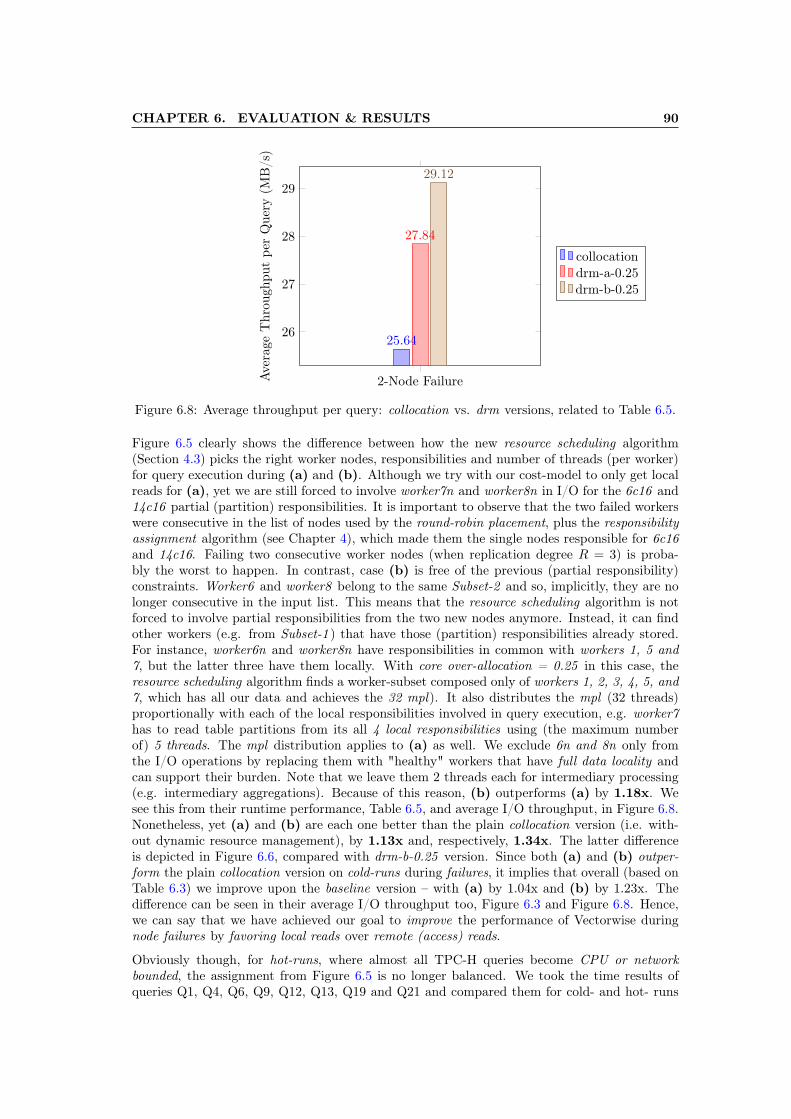
CHAPTER 6. EVALUATION & RESULTS 90
2-Node Failure
26
27
28
29
25.64
27.84
29.12
Average
Throu
ghpu
tpe
rQuery
(MB/s)
collocationdrm-a-0.25drm-b-0.25
Figure 6.8: Average throughput per query: collocation vs. drm versions, related to Table 6.5.
Figure 6.5 clearly shows the difference between how the new resource scheduling algorithm(Section 4.3) picks the right worker nodes, responsibilities and number of threads (per worker)for query execution during (a) and (b). Although we try with our cost-model to only get localreads for (a), yet we are still forced to involve worker7n and worker8n in I/O for the 6c16 and14c16 partial (partition) responsibilities. It is important to observe that the two failed workerswere consecutive in the list of nodes used by the round-robin placement, plus the responsibilityassignment algorithm (see Chapter 4), which made them the single nodes responsible for 6c16and 14c16. Failing two consecutive worker nodes (when replication degree R = 3) is proba-bly the worst to happen. In contrast, case (b) is free of the previous (partial responsibility)constraints. Worker6 and worker8 belong to the same Subset-2 and so, implicitly, they are nolonger consecutive in the input list. This means that the resource scheduling algorithm is notforced to involve partial responsibilities from the two new nodes anymore. Instead, it can findother workers (e.g. from Subset-1 ) that have those (partition) responsibilities already stored.For instance, worker6n and worker8n have responsibilities in common with workers 1, 5 and7, but the latter three have them locally. With core over-allocation = 0.25 in this case, theresource scheduling algorithm finds a worker-subset composed only of workers 1, 2, 3, 4, 5, and7, which has all our data and achieves the 32 mpl). It also distributes the mpl (32 threads)proportionally with each of the local responsibilities involved in query execution, e.g. worker7has to read table partitions from its all 4 local responsibilities using (the maximum numberof) 5 threads. The mpl distribution applies to (a) as well. We exclude 6n and 8n only fromthe I/O operations by replacing them with "healthy" workers that have full data locality andcan support their burden. Note that we leave them 2 threads each for intermediary processing(e.g. intermediary aggregations). Because of this reason, (b) outperforms (a) by 1.18x. Wesee this from their runtime performance, Table 6.5, and average I/O throughput, in Figure 6.8.Nonetheless, yet (a) and (b) are each one better than the plain collocation version (i.e. with-out dynamic resource management), by 1.13x and, respectively, 1.34x. The latter differenceis depicted in Figure 6.6, compared with drm-b-0.25 version. Since both (a) and (b) outper-form the plain collocation version on cold-runs during failures, it implies that overall (based onTable 6.3) we improve upon the baseline version – with (a) by 1.04x and (b) by 1.23x. Thedifference can be seen in their average I/O throughput too, Figure 6.3 and Figure 6.8. Hence,we can say that we have achieved our goal to improve the performance of Vectorwise duringnode failures by favoring local reads over remote (access) reads.
Obviously though, for hot-runs, where almost all TPC-H queries become CPU or networkbounded, the assignment from Figure 6.5 is no longer balanced. We took the time results ofqueries Q1, Q4, Q6, Q9, Q12, Q13, Q19 and Q21 and compared them for cold- and hot- runs

CHAPTER 6. EVALUATION & RESULTS 91
separately, in Figure 6.7. During cold-runs (Figure 6.7a) all these queries are I/O bounded andso, drm-b-0.25 performs the best. On the other hand, during hot-runs (Figure 6.7b) we exhibitthe opposite – Q1, Q4, Q6, and Q12 are now CPU bounded, whereas the remaining Q9, Q13,Q19 and Q21 are network bounded. These 8 queries (and especially the latter 4) have the worsedegrading performance for the drm versions during the hot-run. For example, because of theassignment from Figure 6.5, workers 4, 5, and 7 are now a bottleneck during query executionin drm-b-0.25. This is a tradeoff that the before-mentioned approach has to deal with it duringthe timespan of HDFS data recovery. We could diminish this imbalance effect by increasing thecore over-allocation (e.g. 0.5 over-allocation) and the degree of partitioning (e.g. 32 partitions),it should provide the new resource scheduling algorithm more flexibility in balancing the mplover the chose worker-subset. Nevertheless, for the previous experiment, it takes around 8-9minutes to recover the 3rd missing (approximately 26 GB of data) replicas. This time can beeasily amortized considering the side effect of controlling data-locality, i.e. reading local dataduring cold-runs or when is not enough buffer pool to cache all the tables.
YARN Integration
As we mentioned earlier in this section, we are now going to present the performance results ofthe Vectorwise on Hadoop database system when internal workloads overlap with concurrent(Hadoop) external workloads over the same worker nodes / cluster resources. Hence, we fo-cus on the improvements brought by the dynamic resource scheduling approach (implicitly themin-cost flow algorithm, plus our cost model) and YARN integration for cluster awareness andresource management, while simulating Hadoop busyness over the worker-set with the TeraSortbenchmark. To remember the essentials, we recommend looking into Section 4.3. Summarizing,the approach dynamically schedules cluster compute resources according to the worker-set re-source availability, load-balancing constraints, and data-locality. This should reduce the overallresource contention that exhibits when two or more running systems, coexisting on the samecluster, are not aware of each others workloads. As we pointed out at the end of Section 6.1,we can configure our TeraSort (Hadoop) workloads to run with 16, 32, or 64 mappers andreducers, either on the full worker-set, or on just on a half of it (both with their own input datadirectory). Extra details (i.e. total runtime, CPU load) are given in Table 6.2.
In Tables 6.7, 6.8 and 6.9 we present the runtime results of executing a sequence of 11x TPC-HQ1 and Q13 queries in Vectorwise on Hadoop, with and without YARN integration, side byside with each of the 6 workload combinations (started first), but only for the 100GB data-set because our purpose is to increase the Map phase duration and to prolong the resourcecontention. We also ran the same experiment without any busyness, Table 6.2, to have a baselinefor comparison and also to highlight the resource allocation overhead that shows up at thebeginning of each test. The correspondent assignments of workers, (partition) responsibilitiesand threads per node (out of max available for Vectorwise) involved in query execution duringthe no-busyness, 16M/16R, 32M/32R, and 64M/64R half-set runs are depicted in Figure 6.9,Figure 6.10, Figure 6.11, and respectively, Figure 6.12. Before each of the experiments we clearthe File System’s and buffers manager’s caches and execute a no-busyness cold-run, Figure 6.9tells us what responsibilities are "hot" before the tests. By doing this we can measure theperformance degradation of drmy when its runtime assignment dynamically changes because ofthe cluster’s busyness and thus, "cold" partitions are being read from the disk. In our tableswe show both the results when drmy’s buffers are "semi-hot" (not. drmy-) for the experimentand "hot" (not. drmy+) as well. Note that from the drmy- time results we have excluded theoverhead of allocating resources.
In the end of this section we measure the average CPU load (not. from [min to Max]) ofthe Vectorwise workers on which both internal and external workloads overlap during the Mapphase, Figure 6.13 and Figure 6.14; we can identify that by looking at the assignment figuresbelow the tables (i.e. if max available cores for Vectorwise < max worker capability, which is 16
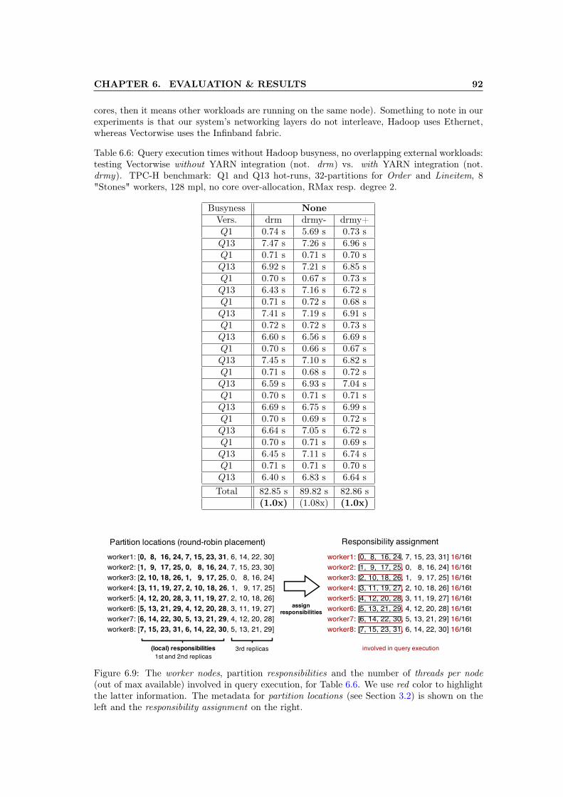
CHAPTER 6. EVALUATION & RESULTS 92
cores, then it means other workloads are running on the same node). Something to note in ourexperiments is that our system’s networking layers do not interleave, Hadoop uses Ethernet,whereas Vectorwise uses the Infinband fabric.
Table 6.6: Query execution times without Hadoop busyness, no overlapping external workloads:testing Vectorwise without YARN integration (not. drm) vs. with YARN integration (not.drmy). TPC-H benchmark: Q1 and Q13 hot-runs, 32-partitions for Order and Lineitem, 8"Stones" workers, 128 mpl, no core over-allocation, RMax resp. degree 2.
Busyness NoneVers. drm drmy- drmy+Q1 0.74 s 5.69 s 0.73 sQ13 7.47 s 7.26 s 6.96 sQ1 0.71 s 0.71 s 0.70 sQ13 6.92 s 7.21 s 6.85 sQ1 0.70 s 0.67 s 0.73 sQ13 6.43 s 7.16 s 6.72 sQ1 0.71 s 0.72 s 0.68 sQ13 7.41 s 7.19 s 6.91 sQ1 0.72 s 0.72 s 0.73 sQ13 6.60 s 6.56 s 6.69 sQ1 0.70 s 0.66 s 0.67 sQ13 7.45 s 7.10 s 6.82 sQ1 0.71 s 0.68 s 0.72 sQ13 6.59 s 6.93 s 7.04 sQ1 0.70 s 0.71 s 0.71 sQ13 6.69 s 6.75 s 6.99 sQ1 0.70 s 0.69 s 0.72 sQ13 6.64 s 7.05 s 6.72 sQ1 0.70 s 0.71 s 0.69 sQ13 6.45 s 7.11 s 6.74 sQ1 0.71 s 0.71 s 0.70 sQ13 6.40 s 6.83 s 6.64 sTotal 82.85 s 89.82 s 82.86 s
(1.0x) (1.08x) (1.0x)
Figure 6.9: The worker nodes, partition responsibilities and the number of threads per node(out of max available) involved in query execution, for Table 6.6. We use red color to highlightthe latter information. The metadata for partition locations (see Section 3.2) is shown on theleft and the responsibility assignment on the right.
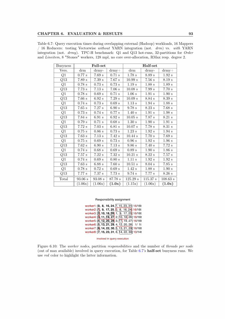
CHAPTER 6. EVALUATION & RESULTS 93
Table 6.7: Query execution times during overlapping external (Hadoop) workloads, 16 Mappers/ 16 Reducers: testing Vectorwise without YARN integration (not. drm) vs. with YARNintegration (not. drmy). TPC-H benchmark: Q1 and Q13 hot-runs, 32-partitions for Orderand Lineitem, 8 "Stones" workers, 128 mpl, no core over-allocation, RMax resp. degree 2.
Busyness Full-set Half-setVers. drm drmy- drmy+ drm drmy- drmy+Q1 0.77 s 7.69 s 0.71 s 1.78 s 8.89 s 1.92 sQ13 7.89 s 7.39 s 7.67 s 10.99 s 7.56 s 8.19 sQ1 0.78 s 0.73 s 0.73 s 1.19 s 1.88 s 1.89 sQ13 7.73 s 7.13 s 7.06 s 10.08 s 7.99 s 7.70 sQ1 0.78 s 0.69 s 0.71 s 1.06 s 1.91 s 1.90 sQ13 7.66 s 6.92 s 7.29 s 10.09 s 8.84 s 8.39 sQ1 0.74 s 0.73 s 0.69 s 1.13 s 1.94 s 1.88 sQ13 7.65 s 7.27 s 6.90 s 9.78 s 8.23 s 7.68 sQ1 0.73 s 0.74 s 0.77 s 1.40 s 1.91 s 1.98 sQ13 7.84 s 6.91 s 6.92 s 10.05 s 7.87 s 8.21 sQ1 0.79 s 0.71 s 0.68 s 1.30 s 1.90 s 1.91 sQ13 7.72 s 7.03 s 6.81 s 10.07 s 7.78 s 8.31 sQ1 0.75 s 0.86 s 0.73 s 1.23 s 1.92 s 1.94 sQ13 7.63 s 7.13 s 7.42 s 10.44 s 7.70 s 7.69 sQ1 0.75 s 0.69 s 0.73 s 0.96 s 1.92 s 1.96 sQ13 7.62 s 6.90 s 7.13 s 9.86 s 7.40 s 7.72 sQ1 0.74 s 0.68 s 0.69 s 0.89 s 1.90 s 1.86 sQ13 7.57 s 7.22 s 7.32 s 10.21 s 8.22 s 7.57 sQ1 0.74 s 0.69 s 0.80 s 1.11 s 1.92 s 1.92 sQ13 7.63 s 6.88 s 7.60 s 10.51 s 8.04 s 7.85 sQ1 0.78 s 0.72 s 0.69 s 1.42 s 1.88 s 1.90 sQ13 7.77 s 7.37 s 7.73 s 9.74 s 7.77 s 8.26 sTotal 93.06 s 93.08 s 87.78 s 125.29 s 115.37 s 108.63 s
(1.06x) (1.06x) (1.0x) (1.15x) (1.06x) (1.0x)
Figure 6.10: The worker nodes, partition responsibilities and the number of threads per node(out of max available) involved in query execution, for Table 6.7’s half-set busyness runs. Weuse red color to highlight the latter information.

CHAPTER 6. EVALUATION & RESULTS 94
Table 6.8: Query execution times during overlapping external (Hadoop) workloads, 32 Mappers/ 32 Reducers: testing Vectorwise without YARN integration (not. drm) vs. with YARNintegration (not. drmy). TPC-H benchmark: Q1 and Q13 hot-runs, 32-partitions for Orderand Lineitem, 8 "Stones" workers, 128 mpl, no core over-allocation, RMax resp. degree 2.
Busyness Full-set Half-setVers. drm drmy- drmy+ drm drmy- drmy+Q1 0.96 s 7.20 s 1.05 s 1.76 s 18.47 s 1.94 sQ13 8.75 s 7.80 s 7.40 s 9.91 s 15.13 s 7.82 sQ1 0.89 s 0.99 s 1.09 s 1.89 s 1.90 s 1.88 sQ13 8.37 s 7.82 s 7.88 s 8.84 s 7.91 s 7.62 sQ1 0.83 s 0.99 s 1.00 s 1.28 s 1.96 s 1.97 sQ13 8.00 s 8.00 s 7.83 s 8.56 s 8.11 s 7.55 sQ1 0.84 s 1.03 s 1.00 s 0.80 s 1.88 s 1.93 sQ13 8.30 s 8.05 s 7.92 s 8.33 s 8.53 s 7.53 sQ1 0.87 s 1.02 s 1.03 s 1.05 s 1.91 s 1.92 sQ13 8.33 s 7.95 s 7.84 s 8.55 s 8.94 s 7.48 sQ1 0.88 s 1.01 s 1.01 s 0.79 s 1.92 s 1.90 sQ13 8.18 s 8.01 s 7.86 s 8.86 s 8.50 s 7.96 sQ1 0.88 s 1.01 s 1.04 s 0.73 s 1.91 s 1.80 sQ13 8.15 s 7.93 s 7.70 s 8.05 s 7.99 s 7.10 sQ1 0.87 s 1.02 s 1.00 s 0.93 s 1.94 s 1.88 sQ13 8.16 s 7.63 s 7.67 s 8.04 s 6.74 s 6.82 sQ1 0.89 s 1.03 s 1.04 s 0.77 s 1.86 s 1.88 sQ13 8.10 s 7.77 s 7.64 s 8.16 s 7.20 s 6.78 sQ1 0.90 s 1.02 s 1.09 s 0.81 s 1.95 s 1.90 sQ13 8.10 s 7.58 s 7.81 s 8.06 s 6.50 s 7.01 sQ1 0.81 s 1.01 s 1.03 s 0.88 s 1.87 s 1.89 sQ13 8.10 s 7.32 s 7.53 s 8.41 s 6.67 s 6.76 sTotal 100.16 s 103.19 s 96.46 s 105.46 s 129.79 s 101.32 s
(1.03x) (1.06x) (1.0x) (1.04x) (1.28x) (1.0x)
Figure 6.11: The worker nodes, partition responsibilities and the number of threads per node(out of max available) involved in query execution, for Table 6.8’s half-set busyness runs. Weuse red color to highlight the latter information.

CHAPTER 6. EVALUATION & RESULTS 95Tab
le6.9:
Query
executiontimes
during
overlapp
ingexternal
(Had
oop)
workloads,64
Map
pers
/64
Reducers:
testingVectorw
isewithout
YARN
integration(not.drm)vs.withYARN
integration(not.drmy).TPC-H
benchm
ark:
Q1an
dQ13
hot-runs,3
2-pa
rtitions
forOrder
andLineitem,8
"Stones"
workers,1
28mpl,n
ocore
over-allo
cation
,RMax
resp.degree
2.
Busyn
ess
Full-set
Half-set
Vers.
drm
drmy-
drmy+
drm
drmy-
(#1)
drmy+
(#1)
drmy-
(#2)
drmy+
(#2)
Q1
1.29
s9.03
s2.07s
6.92s
46.30s
2.48s
44.35s
1.94s
Q13
13.26s
9.09
s9.52s
63.91s
33.81s
14.38s
32.94s
11.25s
Q1
1.34
s1.93
s1.98s
5.59s
1.99s
2.08s
1.92s
1.99s
Q13
12.37s
9.20
s9.53s
21.10s
11.45s
14.11s
10.02s
11.07s
Q1
1.37
s1.89
s2.02s
5.84s
1.97s
2.12s
1.89s
1.93s
Q13
11.58s
8.04
s8.62s
11.17s
11.49s
16.71s
9.98s
10.55s
Q1
1.16
s1.91
s1.95s
2.83s
1.94s
2.88s
1.91s
1.99s
Q13
12.08s
7.23
s7.87s
8.53s
11.31s
10.60s
10.12s
10.64s
Q1
1.68
s2.00
s1.89s
1.03s
1.94s
1.92s
1.98s
1.97s
Q13
8.25
s5.76
s6.69s
8.31s
10.28s
10.58s
9.97s
10.31s
Q1
0.83
s2.07
s2.12s
0.89s
1.96s
1.95s
1.91s
1.93s
Q13
8.31
s5.39
s5.23s
8.98s
10.34s
9.83s
9.95s
10.35s
Q1
0.88
s2.04
s2.12s
0.80s
1.95s
2.00s
1.93s
1.94s
Q13
8.54
s5.25
s5.31s
8.48s
10.18s
10.77s
10.09s
10.32s
Q1
0.81
s2.08
s2.09s
0.87s
1.92s
1.96s
1.89s
1.94s
Q13
7.99
s6.05
s5.58s
8.16s
10.71s
10.00s
10.25s
10.57s
Q1
0.86
s2.07
s2.11s
0.87s
1.95s
1.95s
1.90s
1.95s
Q13
8.56
s5.35
s5.38s
8.62s
10.92s
10.33s
9.96s
10.30s
Q1
1.05
s2.04
s1.99s
0.85s
1.91s
1.94s
1.87s
2.06s
Q13
8.49
s6.75
s4.73s
8.63s
10.28s
10.10s
9.94s
10.92s
Q1
0.89
s1.93
s2.02s
1.05s
1.89s
1.94s
1.88s
2.00s
Q13
8.29
s6.73
s4.67s
8.88s
10.76s
11.06s
10.06s
10.76s
Total
119.88
s103.83s
95.49s
192.31s
207.25s
151.69s
196.71s
138.68s
Full-set
(1.25x
)(1.08x
)(1.0x)
––
––
–Half-set(1)
––
–(1.26x
)(1.36x
)(1.0x)
––
Half-set(2)
––
–(1.38x
)–
–(1.41x
)(1.0x)
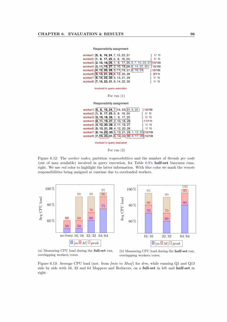
CHAPTER 6. EVALUATION & RESULTS 96
For run (1)
For run (2)
Figure 6.12: The worker nodes, partition responsibilities and the number of threads per node(out of max available) involved in query execution, for Table 6.9’s half-set busyness runs.right. We use red color to highlight the latter information. With blue color we mark the remoteresponsibilities being assigned at runtime due to overloaded workers.
no-busy.16/16 32/32 64/64
60%
80%
100%
60
90 9095
60 60
70
90
50 50
60
75
Avg
CPU
load
[m M ] peak
(a) Measuring CPU load during the full-set run,overlapping workers/cores.
16/16 32/32 64/64
60%
80%
100% 9590
100
80
70
95
70
60
80
Avg
CPU
load
[m M ] peak
(b) Measuring CPU load during the half-set run,overlapping workers/cores.
Figure 6.13: Average CPU load (not. from [min to Max]) for drm, while running Q1 and Q13side by side with 16, 32 and 64 Mappers and Reducers, on a full-set in left and half-set inright.

CHAPTER 6. EVALUATION & RESULTS 97
no-busy.16/16 32/32 64/64
60%
80%
100%
60
70
80
90
60
70
8085
50
60 60
70
Avg
CPU
load
[m M ] peak
(a) Measuring CPU load during the full-set run,non-overlapping resources.
16/16 32/32 64/64
60%
80%
100%
80
70 7070 70
6060 60
50
Avg
CPU
load
[m M ] peak
(b) Measuring CPU load during the half-set(#1) run, non-overlapping resources.
Figure 6.14: Average CPU load (not. from [min to Max]) for drmy, while running Q1 and Q13side by side with 16, 32 and 64 Mappers and Reducers, on a full-set in left and half-set inright.
For the result discussion, we start with our full-set runs. For these tests, drmy (with YARNintegration and, implicitly, with the new resource scheduling algorithm) uses the same assign-ment as if the cluster had no busyness, that is the assignment from Figure 6.9. Our full-setTeraSort jobs are using the full-set of workers in a balanced manner, i.e. 2, 4 and 8 M/R pernode, hence the runtime assignment (i.e. the resource footprint) has to be balanced as well.The only thing that differs, compared with drm that had no YARN awareness, is the mpl thatwe try to achieve when different workloads overlap on the same set of resources. Because drmyis aware that our CPU available resources are much lower during each 16, 32 to 64 M/R test, itdecreases the mpl from 128 (w/o busyness) to 128 - 17 = 111, 128 - 33 = 95 and, respectively,128 - 65 = 63 threads. In this situation, the algorithm acts more as a throttling mechanism.As we can see from the 64M/64R drm tests, for the first 10 queries or so (exactly while theMap phase of TeraSort happens) the performance degrades, i.e. spikes to 95% in the CPU load.This does not happen to the drmy version for instance, or if it happens is affecting Vectorwiseless. It is important to mention that 1 core is used by the TeraSort (managed) ApplicationMaster and this actually used to influence our experiments for the full-set runs, i.e. the core isallocated and it appears so in YARN, but never used intensively as such. We had to literallyforce our algorithms to ignore this glitch when deciding the resource footprint at runtime. Yet,overall, we achieve better results compared with the drm version (w/o YARN integration).Tables 6.7, 6.8 and 6.9 show better (individual and total) times for the 11x Q1,Q13 workload,though we suffer a lot due to the allocation overhead as seen in the first query’s time result.Also, few to non-existent CPU peaks are recorded during the full-set runs for drmy, Figure 6.14,as compared to drm in Figure 6.13. Note that in all our drmy tests we do not have overlappingresources (i.e. each workload, internal and external, uses its own reserved resources). The CPUload measurements were done for those cores allocated exclusively to Vectorwise on the workernodes which also happened to run a small part of the external Hadoop workload. Hence, isperfectly normal for the CPU load to be somewhat bigger compared to a normal (w/o anybusyness) run given that we read and process the same amount of data, but on less cores (andimplicitly with less parallelism).
For the half-set tests we are just going to focus on the 64M/64R runs, as the others (with16M/16R and 32M/32R) exhibit the same behavior. We start by noticing the same contentionproblem with the drm version, which also occurred in the full-set runs. During the first 80-90sof our half-set runs (i.e. the first 8 queries or so) the external workload’s Map phase severely
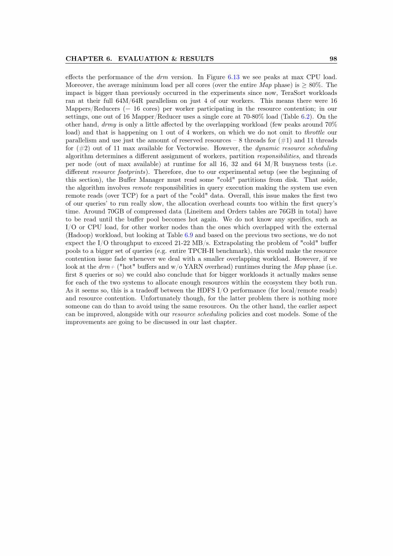
CHAPTER 6. EVALUATION & RESULTS 98
effects the performance of the drm version. In Figure 6.13 we see peaks at max CPU load.Moreover, the average minimum load per all cores (over the entire Map phase) is ≥ 80%. Theimpact is bigger than previously occurred in the experiments since now, TeraSort workloadsran at their full 64M/64R parallelism on just 4 of our workers. This means there were 16Mappers/Reducers (= 16 cores) per worker participating in the resource contention; in oursettings, one out of 16 Mapper/Reducer uses a single core at 70-80% load (Table 6.2). On theother hand, drmy is only a little affected by the overlapping workload (few peaks around 70%load) and that is happening on 1 out of 4 workers, on which we do not omit to throttle ourparallelism and use just the amount of reserved resources – 8 threads for (#1) and 11 threadsfor (#2) out of 11 max available for Vectorwise. However, the dynamic resource schedulingalgorithm determines a different assignment of workers, partition responsibilities, and threadsper node (out of max available) at runtime for all 16, 32 and 64 M/R busyness tests (i.e.different resource footprints). Therefore, due to our experimental setup (see the beginning ofthis section), the Buffer Manager must read some "cold" partitions from disk. That aside,the algorithm involves remote responsibilities in query execution making the system use evenremote reads (over TCP) for a part of the "cold" data. Overall, this issue makes the first twoof our queries’ to run really slow, the allocation overhead counts too within the first query’stime. Around 70GB of compressed data (Lineitem and Orders tables are 76GB in total) haveto be read until the buffer pool becomes hot again. We do not know any specifics, such asI/O or CPU load, for other worker nodes than the ones which overlapped with the external(Hadoop) workload, but looking at Table 6.9 and based on the previous two sections, we do notexpect the I/O throughput to exceed 21-22 MB/s. Extrapolating the problem of "cold" bufferpools to a bigger set of queries (e.g. entire TPCH-H benchmark), this would make the resourcecontention issue fade whenever we deal with a smaller overlapping workload. However, if welook at the drm+ ("hot" buffers and w/o YARN overhead) runtimes during the Map phase (i.e.first 8 queries or so) we could also conclude that for bigger workloads it actually makes sensefor each of the two systems to allocate enough resources within the ecosystem they both run.As it seems so, this is a tradeoff between the HDFS I/O performance (for local/remote reads)and resource contention. Unfortunately though, for the latter problem there is nothing moresomeone can do than to avoid using the same resources. On the other hand, the earlier aspectcan be improved, alongside with our resource scheduling policies and cost models. Some of theimprovements are going to be discussed in our last chapter.

Conclusions
Contributions
In this Master’s thesis we undertook the challenge of creating the groundwork towards enablingdynamic resource management in Vectorwise on Hadoop MPP database system. The milestoneswe tried to reach were deciding on the high-level system architecture and creating a proof ofconcept that demonstrates (1) improved data-locality, (2) better performance and reliabilityduring node failures, as well as (3) the ability to cope with overlapping external (Hadoop)workloads, all due to our custom HDFS block replication policy, min-cost flow algorithms(plus cost-models) for dynamic resource scheduling, and YARN-integration for cluster resourcemanagement. Thereby, we consider that we achieved (to a certain extent) all our research goalsfrom Section 1.5.
Answers to Our Research Questions
Scheduling and resource management are not only important, but also very challenging. Clus-ters are exposed to a wide range of applications, that have highly diverse characteristics andperformance requirements. For example, Map-Reduce applications are usually characterized bylong running jobs. These jobs desire shorter turnaround time - time from submission to com-pletions. Queries in database systems for analytical or transactional workloads, on the otherhand, are much shorter-lived and much more interactive. Further, these environments need tosupport a large number of users simultaneously. As a result, the underlying system needs torespond to these kind of workloads as soon as they arrive, even at the cost of stretching theiroverall turnaround time slightly. Managing both types of workloads at the same time makesit even more difficult for a cluster resource manager, especially when each workload belongs toa different applications (e.g. running Map-Reduce jobs and OLAP queries). Scheduling andresource management needs to take numerous system parameters, such as CPU speed, memorysize, I/O bandwidth, network bandwidth, context switch overhead, etc, into account. Thesemetrics are often inter-related and can affect the choice of an effective scheduling strategy.
Coming back to our initial research questions, we argue that with an easy, non-intrusive designand only by using the existing meanings, i.e. YARN and HDFS native APIs, X100’s existingcode base, etc., it is still possible to implement dynamic resource management into Vectorwiseon Hadoop. Besides the current API big issues regarding YARN’s container resource extensionand its inability as a service to monitor in real time an extensive set of metrics, other thanCPU and memory availability, perhaps our major limitation has to do with the latter problemof effective scheduling. Though the min-cost flow approach has proven to be a viable option inliterature for resource management and scheduling purposes, the cost-models we use flattensthe relationship between the numerous system parameters, which means that we normalizebeforehand all our cost values to the same "nominator". This makes it even harder for us todefine relationships between different metrics or prioritize some of them more than the others.
99

CHAPTER 6. EVALUATION & RESULTS 100
Future Work
Apart from the enhancement opportunities we identified and implemented during this project,we also envision and address the challenge of providing in the near future the following featuresand improvements to our master’s thesis approach.
Perfecting the cost-models
Since both the worker-set selection (Section 4.1) and responsibility assignment (Section 4.2) areperformed only once at database startup and work with (more ore less) static system properties,we cannot improve by a lot the cost-models for these algorithms. What we can rather do is toaccount for a few more YARN metrics in our formulas, such as disk speed, network bandwidth,etc., whenever they are made available in the API. However, besides the latter additions of newmetrics, for the dynamic resource scheduling (Section 4.3) algorithm we propose the followingimprovements that could bring it to completion:
• When defining the penalty cost for partial responsibilities (i.e. not yet local partitions),have instead a value that corresponds to how much from that partition was replicatedlocally already; it could be a percentage value (e.g. 80% replicated) that is normalizedcorrespondingly to our cost-model (e.g. cost of 0.8). Overall this would make the cost-model take smarter decisions.
• We could also take in account the historical information about what (partition) respon-sibilities were involved during query execution and introduce another layer of costs, e.g.hot responsibilities, as they become "hot" in the buffer. With this we can alter a bit ourcost-model and avoid hitting the disk to overcome Hadoop’s local I/O poor performance.However, it would be hard to know when partitions are evicted from the buffer pool, suchthat we change our costs from hot to local again. We do something similar for respon-sibility assignment, where we account in the cost-model for ex-responsibilities (labeledas local+, instead of local-) that could have been cached by the worker node’s OS FileSystem. But there, data caching is just a side-effect and no assumptions can be made inthat sense. The File System’s cache is not under our control, whereas the Buffer Manageris.
• Last but not least, is to try to achieve some data-locality for remote responsibilities whenwe must involve them in query execution. The idea is to differentiate the penalty costsof remote responsibilities that match locally with some worker’s [RMax, . . . , R] intervalof remaining replicas from those who do not (R replication factor, RMax responsibilitydegree). It will be transparent for the resource scheduling algorithm as remote responsi-bilities will still be considered as such. Nevertheless, in this way we can extend our viewtowards all R replicas without increasing the RMax degree and overloading the workernodes with an extra degree of responsibility.
Full resource elasticity within a Hadoop cluster
To achieve full resource elasticity within a Hadoop cluster we still need to revise our approachfor a neat YARN integration and to perfect the internal Vectorwise workload monitoring, along-side with our resource management policies. We devise the work that has to be done in twodirections, each one with its own roadmap of alternative ideas for improvements:

CHAPTER 6. EVALUATION & RESULTS 101
YARN integration
As stated in YARN-896 1, there is significant work ongoing to allow long-lived services run-ning as YARN applications. For example, the API’s functionality to increase/decrease resourceutilization within YARN containers (YARN-1197 2) is not yet implemented. This makes itimpossible "per se" to gain full elasticity and to allocate/deallocate resources in a fine-grainedfashion for Vectorwise. Though the idea to model resource requests as separate YARN ap-plications (Section 5.1) achieves elasticity to a certain extent for increasing the amount ofresources, we saw that is limited when it comes to the opposite operation, decreasing resources.We cannot just deallocate the difference of resources between different overlapping workloadsby just using the available API interface. With the existing YARN release this functionalitywould be translated into (1) stopping the existent Application Master (for the first workload)and then (2) starting another one (for the second workload), which adds a significant overheadand is not a worthwhile solution to implement from a product-wise point of view. Therefore,our workaround for the moment is to release all requested resources at once, when the latestworkload ends (idle state duration > threshold) and there are no other queries still active inthe system.
However, with YARN-1197 being pushed in a next release, we plan to revise our approach in thefuture. For instance, instead of creating one YARN Application Master per resource request (perworkload), we could multiplex all the requests towards a single YARN Application Master (or apool of applications distributed over different scheduling queues) that is delegated to Vectorwiseand can dynamically increase/decrease the amount of resources for its own containers. Therebywe can avoid the application startup overhead entirely and reduce the request latency even more(i.e. a YARN Application Master can run in background and listen only for new requests).
A second idea could be to use Apache’s Slider 3 platform, launched in beta-version aroundJune 2014, which exposes a set of services that allow long-running applications, real-time andonline applications to easily integrate into YARN (and be YARN-Ready 4). Besides, it providesan interface for real-time communication, especially for database systems running on Hadoopor database-style workloads where a very high-speed transfer or data processing and responsetimes are required. It complements Apache Tez 5, which is quickly gaining adoption as thebatch and interactive engine of Hadoop. However, one thing to note, is that Slider, as well asthe YARN 2.2 release, do not support resource extension (i.e. increase or decrease primitives)for containers yet. This means we would still need a work-around to achieve resource elasticityfor Vectorwise on Hadoop, to allocate or deallocate resources when is required so.
Another alternative is to use the so called Container Delegation 6, a very new capability thatis being added to YARN. Currently, the Standard Container Model looks as such: a YARNapplication (via the Application Master) negotiates a container from the Resource Managerand then launches the container by interacting with the Node Manager to utilize the allocatedresources (CPU, memory etc.) on the specific machine. Now, YARN-1488 7 is adding a newmodel called the Delegated Container Model. It helps to understand the distinction betweena Service X that is already running in YARN containers or externally such as Vectorwise,and an application that needs to utilize this service, for example a Vectorwise query. In theDelegated Container Model, the query can negotiate containers from the Resource Manager (viathe Application Master) and, rather than launching them to utilize the new allocated resources,it delegates all these resources to Service X instead, which then gets additional resources from
1YARN-896: issues.apache.org/jira/browse/YARN-8962YARN-1197: issues.apache.org/jira/browse/YARN-11973Apache Slider: slider.incubator.apache.org4YARN-Ready Program: hortonworks.com/press-releases/hortonworks-announces-yarn-ready-program5Apache Tez: tez.apache.org6Container Delegation: hortonworks.com/blog/evolving-apache-hadoop-yarn-provide-resource-workload-
management-services/7YARN-1488: issues.apache.org/jira/browse/YARN-1488

CHAPTER 6. EVALUATION & RESULTS 102
its Node Manager(s) to be used on behalf of the query. This scheme contrasts with the StandardContainer Model, basically the only way of building a YARN application today, in which theapplication would launch and manage the containers itself to use the allocated resources. Froman implementation perspective, the Node Manager(s), on delegation, will expand the targetcontainers of Service X, by modifying them to allow for more CPU, memory etc. When thecontainers are no longer needed, Service X can release them back to YARN, so the resourcescan now be used by other applications.
Workload monitor and resource management
An alternative approach to our workload monitor (Section 5.3), which should contribute to ourefforts on achieving full resource elasticity, is as follows. Through specific formulas, at regularintervals we would measure the internal load of the system. An element to the computationwould be to establish whether queries get to a certain target of parallelism level – the currentmaximum parallelism level, or as well a new environment variable such as target parallelism levelor minimum parallelism level. If queries on average get significantly less parallelism than desired(by the target), then the system will be considered overloaded. If they get significantly more,will be classified as underloaded. The workload monitor should respond to this information overtime (i.e. every few minutes), trying via YARN to gradually increase the amount of allocatedresources if the system is "overloaded", or yielding them otherwise (if "underloaded"). Thedescribed alternative for the workload monitor is better mostly in the sense that resourceelasticity would be managed in the background and never influence the latency of an individualresource request. This is a drawback of our current Master’s thesis approach that needs to befixed. Also, our current approach may not be better as such in identifying all the context (seeSection 5.1) changes that determine when to ask YARN for more resources.
Another feature that is not yet supported would be to modify our (custom) HDFS block replica-tion for Vectorwise such that it tries to create R node sets S1, . . . , SR (R the replication degree,e.g. 3) with every Si having each table partition exactly once. This would allow us to put tosleep different node sets. Putting to sleep implies that we maintain the X100 backend processesrunning on the worker nodes, but entirely avoid using these nodes for query execution, and assuch, deregister them from YARN. This means we can still run our database on the N
R workers(N number of nodes) that are awake, and use one core on each as the minimal resource footprint.Note that, assuming C cores per worker node, in the latter situation we are just using 1
C∗RCPU resources. Nonetheless, we can scale all the way up to N ∗ C cores.

Acknowledgements
This thesis was made possible thanks to Actian Corporation, which hosted the project andprovided the necessary development environment (with extra support from Centrum Wiskunde& Informatica), as part of a 8-months internship.
Second, I would like to thank my supervisor, Prof. Dr. Peter Boncz, for his high devotion forthe project, day-by-day guidance and productive discussion sessions. I am also thankful to mysecond reader, Prof. Dr. Henri Bal, for contributing to the final shape of my thesis.
I worked in an open-minded and friendly environment, and I owe this great experience to theentire Vectorwise team in Amsterdam, especially to (in the alphabetical order of their lastname) Andrei Costea, Adrian Ionescu, Bogdan Raducanu, and Michal Szafranski, who alwaystook the time to answer my questions and help me to fulfill the project.
Last but not least, I would like to thank my family and friends for their everlasting support.
Cristi
103
Bibliography
[1] J. Dean and S. Ghemawat. MapReduce: Simplified Data Processing on Large Clusters. InProceedings of the OSDI, 2016.
[2] Parquet columnar storage for Hadoop. blog.cloudera.com/blog/2013/03/introducing-parquet-columnar-storage-for-apache-hadoop
[3] ORC file format for Hadoop. hortonworks.com/blog/orcfile-in-hdp-2-better-compression-better-performance
[4] V. Kumar Vavilapalli et al. Apache Hadoop YARN: Yet Another Resource Negotiator. InProceedings of the SoCC, 2013.
[5] S. Babu and H. Herodotou. Massively Parallel Databases and MapReduce Systems. Foun-dations and Trends in Databases, Vol. 5, 2012
[6] G. Graefe. Volcano - an extensible and parallel query evaluation system. In Proceedings ofthe IEEE Transactions on Knowledge and Data Engineer, 1994.
[7] M Zukowski. Balancing vectorized execution with bandwidth-optimized storage. PhD thesis,Centrum Wiskunde en Informatica (CWI), 2009.
[8] P. Boncz and M. Kersten. MIL primitives for querying a fragmented world. In Proceedingsof the VLDB Journal, 1999.
[9] P. Boncz, M. Zukowski, and N. Nes. MonetDB/X100: Hyper-Pipelining Query Execution.In Proceedings of CIDR, 2005.
[10] S. Padmanabhan, T. Malkemus, R. Agarwal, and A. Jhingran. Block Oriented Processingof Relational Database Operations in Modern Computer Architectures. In Proceedings ofthe IEEE ICDE, 2001.
[11] M. Zukowski, P. A. Boncz, N. J. Nes, and S. Heman. Monetdb/X100 - A DBMS In TheCPU Cache. IEEE Data Engineering Bulletin, 2005.
[12] Kenneth C. Sevcik. Application scheduling and processor allocation in multiprogrammedparallel processing systems. In Performance Evaluation, 19:107 140, 1994.
[13] E. Rahm. Dynamic load balancing in parallel database systems. 1995.
[14] H. Märtens, E. Rahm, and T. Stöhr. Dynamic query scheduling in parallel data warehouses.In Proceedings of the 8th International Euro-Par Conference on Parallel Processing, Euro-Par, 2002.
[15] E. Rahm. Parallel query processing in shared disk database systems. 1993.
[16] A. Thusoo, J. S. Sarma, N. Jain, Z. Shao, P. Chakka, N. Zhang, S. Antony, H. Liu, andR. Murthy. Hive - A Petabyte Scale Data Warehouse Using Hadoop. In Proceedings of theIEEE ICDE, 2010.
104

BIBLIOGRAPHY 105
[17] Y. Huai, A. Chauhan, A. Gates, G. Hagleitner, E. N. Hanson, O. O’Malley, J. Pandey, Y.Yuan, R. Lee, and X. Zhang. Major Technical Advancements in Apache Hive., In Proceed-ings of the SIGMOD, 2014.
[18] A. Abouzeid, K. Bajda-Pawlikowski, D. Abadi, A. Silberschatz, and A. Rasin. HadoopDB:an architectural hybrid of MapReduce and DBMS technologies for analytical workloads. InProceedings of the VLDB Endowment, 2009.
[19] A. Abouzied, D. Abadi, and A. Silberschatz. Invisible Loading: Access-Driven Data Trans-fer from Raw Files into Database Systems. In Proceedings of the EDBT/ICDT, 2013.
[20] Hawq whitepaper. Pivotal HD: HAWQ. A true SQL engine for Hadoop.
[21] L. Chang, Z. Wang, T. Ma, L. Jian, L. Ma, A. Goldshuv, L. Lonergan, J. Cohen, C. Welton,G, Sherry and M. Bhandarkar. HAWQ: A Massively Parallel Processing SQL Engine inHadoop. In Proceedings of the SIGMOD, 2014.
[22] EMC Greenplum presentation, F. Was. Beyond Conventional Data Warehousing. Green-plum Inc.
[23] Impala distributed SQL query engine. blog.cloudera.com/blog/2012/10/cloudera-impala-real-time-queries-in-apache-hadoop-for-real
[24] Inside Cloudera Impala: Runtime Code Generation. blog.cloudera.com/blog/2013/02/inside-cloudera-impala-runtime-code-generation/
[25] J. Sompolski, M. Zukowski, and P. Boncz. Vectorization vs. compilation in query execution.In Proceedings of the DaMoN, 2011.
[26] Distributed SQL query engine for big data. prestodb.io
[27] M. Traverso. Presto: Interacting with petabytes of data at Facebook. www.facebook.com/notes/facebook-engineering/presto-interacting-with-petabytes-of-data-at-facebook/10151786197628920
[28] B. Schroeder and M. Harchol-Balter. Achieving class-based QOS for transactional work-loads. In Proceedings of the IEEE ICDE, 2006.
[29] B. Schroeder, M. Harchol-Balter, A. Iyengar, E. Nahum, and A. Wierman. How to deter-mine a good multi-programming level for external scheduling. In Proceedings of the IEEEICDE, 2006.
[30] B. Niu, P. Martin, W. Powley, P. Bird, and R. Horman. Adapting mixed workloads to meetSLOs in autonomic DBMSs. In Proceedings of the IEEE ICDE, 2007.
[31] U. Dayal, H. Kuno, J. L. Wiener, K. Wilkinson, A. Ganapathi, and S. Krompass.Managingoperational business intelligence workloads. In proceedings of the SIGOPS, 2009.
[32] S. Krompass, U. Dayal, H. A. Kuno, and A. Kemper. Dynamic Workload Management forVery Large Data Warehouses: Juggling Feathers and Bowling Balls. In Proceedings of theVLDB Endowment, 2007.
[33] S. Krompass, Harumi A. Kuno, Janet L. Wiener, Kevin Wilkinson, Umeshwar Dayal,and Alfons Kemper. Managing Long-running Queries. In Proceedings of the InternationalConference on Extending Database Technology, ACM, 2009.
[34] Hadoop’s Capacity Scheduler. hadoop.apache.org/core/docs/current/capacity_scheduler.html
[35] M. Zaharia, The Hadoop Fair Scheduler. developer.yahoo.net/blogs/hadoop/FairSharePres.ppt

BIBLIOGRAPHY 106
[36] M. Zaharia, A. Konwinski, A. D. Joseph, R. Katz, I. Stoica. Improving MapReduce Per-formance in Heterogeneous Environments. In Proceedings of the OSDI, 2008.
[37] M. Zaharia, D. Borthakur, J. Sen Sarma, K. Elmeleegy, S. Shenker, and I. Stoica. Delayscheduling: a simple technique for achieving locality and fairness in cluster scheduling. InProceedings of the EuroSys, 2010.
[38] B. Palanisamy, A. Singh, L. Liu, and B. Jain. Purlieus: Locality-aware resource allocationfor MapReduce in a cloud. In Proceedings of the SC, 2011.
[39] M. Li, D. Subhraveti, Ali R. Butt, A. Khasymski, and P. Sarkar. CAM: a topology awareminimum cost flow based resource manager for MapReduce applications in the cloud. InProceedings of the HPDC, 2012.
[40] M. Isard, V. Prabhakaran, J. Currey, U. Wieder, K. Talwar, and A. Goldberg. Quincy:fair scheduling for distributed computing clusters. In Proceedings of the SOSP, 2009.
[41] G. Graefe. Encapsulation of parallelism in the Volcano query processing system. In Pro-ceedings of the SIGMOD, 1990.
[42] E. Parsons and K. C. Sevcik. Multiprocessor scheduling for high-variability service timedistributions. In Scheduling Strategies for Parallel Processing, Lecture Notes in ComputerScience, 1995.
[43] A. Costea, A. Ionescu, Query Optimization and Execution in Vectorwise MPP. MSc thesis,Actian Corp., 2012.
[44] S. Heman, M. Zukowski, N. J. Nes, L. Sidirourgos, P. Boncz. Positional update handlingin column stores. In Proceedings of the SIGMOD, 2010.
[45] T. H. Cormen, C. E. Leiserson, R. L. Rivest. Introduction to Algorithms.
[46] Introduction to Minimum Cost Flows, 15.082J, 6.855J and ESD.78J MIT Courses, October26, 2010. ocw.mit.edu/courses
[47] Parquet presentation: Hadoop Summit 2013. www.slideshare.net/julienledem/parquet-hadoop-summit-2013
[48] Parquet’s 1GB block size, insert [shuffle]. www.cloudera.com/content/cloudera-content/cloudera-docs/Impala/latest/Installing-and-Using-Impala/ciiu_parquet.html
[49] Topcoder. Minimum Cost Flow, Part 2: Algorithms. community.topcoder.com/tc?module=Static&d1=tutorials&d2=minimumCostFlow2
[50] B. Thirumala Rao, N. V. Sridevi, V. Krishna Reddy, L. S. S. Reddy. Performance Issuesof Heterogeneous Hadoop Clusters in Cloud Computing. In Global Journal of ComputerScience and Technology, May 2011.
[51] Set and Partitions: Covering, Hitting, and Splitting. www.nada.kth.se/~viggo/wwwcompendium/node142.html
[52] Weighted set covering problem. en.wikipedia.org/wiki/Set_cover_problem
[53] Konstantinos Vasileiadis. A Proof that Hitting Set is NP-Complete. 2013.
[54] Tien Duc Dinh. Hadoop Performance Evaluation. Research report (practicum stage),Ruprecht-Karls Universitat Heidelberg (Institute of Computer Science), 2009.


![Vrije Universiteit Amsterdam · Blue-green catastrophe: remote sensing of mass viral lysis of cyanobacteria. [Ph. D. Thesis, Vrije Universiteit Amsterdam] In Dutch: Blauwgroene catastrofe:](https://static.fdocuments.in/doc/165x107/612677d57244e22780525e75/vrije-universiteit-amsterdam-blue-green-catastrophe-remote-sensing-of-mass-viral.jpg)